GROUND DISPLACEMENTS AND PIPE RESPONSE DURING

PULLED-IN-PLACE PIPE INSTALLATION

by

Johnathan Andrew Cholewa

A thesis submitted to the Department of Civil Engineering

In conformity with the requirements for

the degree of Doctor of Philosophy

Queen’s University

Kingston, Ontario, Canada

(April, 2009)

Copyright © Johnathan A. Cholewa, 2009

ii

Abstract

Polymer pipes, typically high density polyethylene (HDPE), can be pulled-into-place,

avoiding traditional cut-and-cover construction, using pipe bursting and horizontal directional

drilling (HDD) pipe installation techniques. Of particular interest, are the ground

displacements, induced by cavity expansion, associated with these techniques and the strains

that develop in existing pipes in response to these displacements. Further, the axial stress-

strain response of the new HDPE pipe during and after the cyclic pulling force history

required to pull the pipe into place is of interest.

Surface displacements and strains in an adjacent polyvinyl chloride (PVC) pipe

induced by static pipe bursting were measured during the replacement of a new unreinforced

concrete pipe, buried 1.39 m below the ground surface, within a test pit filled with a well-

graded sand and gravel. For the pipe bursting geometry tested, the maximum vertical surface

displacement measured at the ground surface was 6 mm, while the distribution of vertical

surface displacements extended no more than 2 m on either side of the centreline. The

maximum longitudinal strain measured in the PVC pipe was less than 0.1% and its vertical

diameter decreased by only 0.5%, suggesting that pipe bursting did not jeopardize the long-

term performance of the water pipe tested.

In addition, results from identical stress relaxation and creep tests performed on

whole pipe samples and coupons trimmed from a pipe wall were compared, and these

demonstrated that the coupons exhibited higher modulus than the pipe samples. Therefore,

isolated pipe samples, as opposed to coupons, were tested to quantify the stress-strain

response of HDPE pipe during the simulated installation, strain recovery, and axial restraint

stages of HDD. Axial strains were found to progressively accumulate when an HDPE pipe

iii

sample was subjected to the cyclic stress history used to simulate an HDD installation. It was

shown that existing linear and nonlinear viscoelastic models can serve as predictive design

tools for estimating the cyclic strain history of HDPE pipe during installation. For the

specific conditions examined, the tensile axial stresses redeveloped in the pipe samples, once

restrained, were not large enough to lead to long-term stress conditions conducive to slow

crack growth even when the short-term performance limits were exceeded by a factor of 1.5.

iv

Co-Authorship

All of the work contained in this thesis was co-authored by J. Cholewa and his supervisors

Dr. R.W.I Brachman and Dr. I.D. Moore. In addition, the work presented in Chapter 2 was

co-authored by Dr. W.A. Take. The research reported herein was initiated from consultation

between J. Cholewa, Dr. R.W.I Brachman, and Dr. I.D. Moore. The laboratory testing was

planned by J. Cholewa, Dr. R.W.I Brachman, and Dr. I.D. Moore and performed by J.

Cholewa. Analysis of the results from the laboratory tests was performed by J. Cholewa

under the supervision of Dr. R.W.I Brachman and Dr. I.D. Moore.

v

Acknowledgements

I would like to thank NSERC for providing funding for this research, through a Strategic

Research Grant on pulled in place pipe installation. In addition, I would like to acknowledge

KWH Pipe Canada for supplying the pipe samples used for this project.

I wish to thank my supervisors, Dr. Richard Brachman and Dr. Ian Moore, for their

guidance during this research project and for training me to think outside the box. Working

with the two of you has been an enjoyable experience.

The contributions of Brandon Taylor with the set-up of the experiments in Chapters 3

and 4 and Dr. Andy Take with the design of the PIV system are gratefully acknowledged. I

would also like to acknowledge the assistance provided by the Department of Civil

Engineering’s support staff.

The friendships I made were a big part of my experience during graduate school and I

would like to thank Steve Vardy, Simon Dickinson, Michael Ranger, and Jeff Hachey for

prolonging this process.

I would like to thank my father Peter for taking me to work in grade 9 and

introducing me to the engineering profession, my mother Maureen for her ongoing support

and love, and my brothers and sisters Peter, Jess, Matthew, Dan, Chris, Jeff, Kathryn, and

Michael. I have been very fortunate to have acquired such wonderful in-laws Warren and

Debbie; I appreciate all they have done to make my life easier so I could focus on my studies.

Finally, a special thanks to my wonderful wife Susan for many things including her

understanding, encouragement, and support (both emotional and financial) during the last

few years. I am looking forward to the next stage of our life together.

vi

Table of Contents

Abstract ....................................................................................................................................ii Co-Authorship ........................................................................................................................iv Acknowledgements ..................................................................................................................v Table of Contents....................................................................................................................vi List of Tables............................................................................................................................x List of Figures .........................................................................................................................xi Chapter 1 Introduction ...........................................................................................................1

1.1 Description of problem....................................................................................................1 1.1.1 State of existing pipelines .........................................................................................1 1.1.2 Pipe bursting .............................................................................................................1 1.1.3 Horizontal directional drilling ..................................................................................3

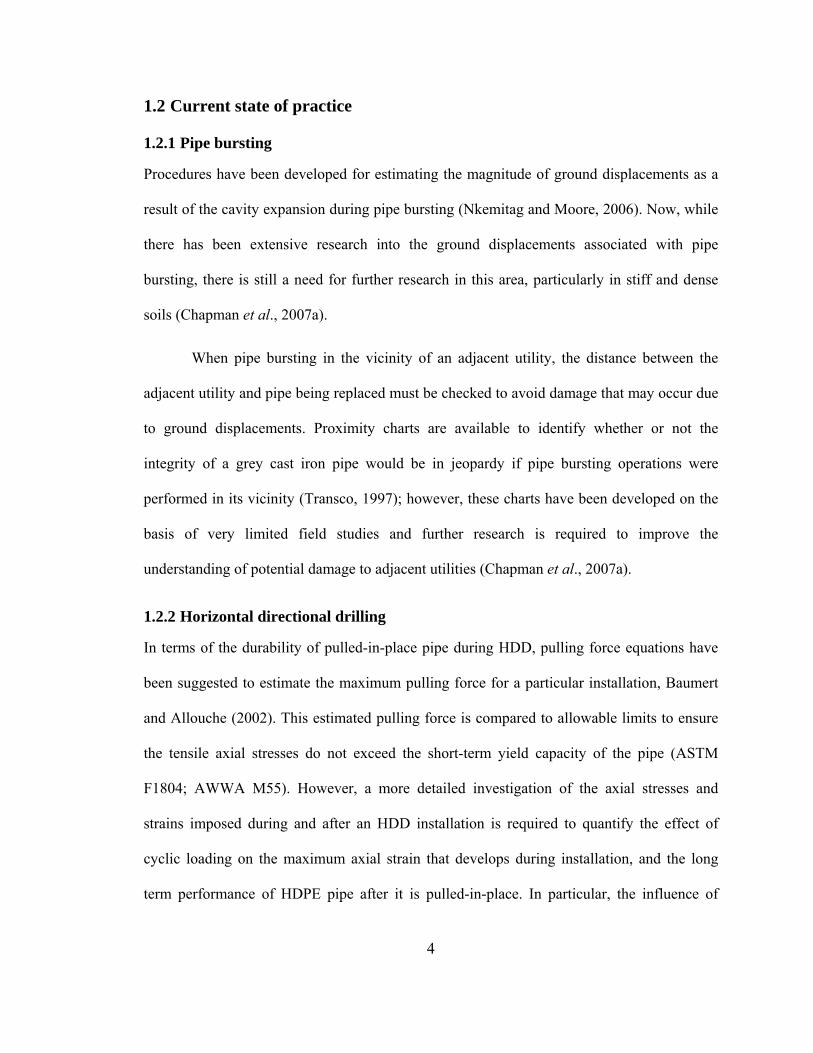
1.2 Current state of practice...................................................................................................4 1.2.1 Pipe bursting .............................................................................................................4 1.2.2 Horizontal directional drilling ..................................................................................4

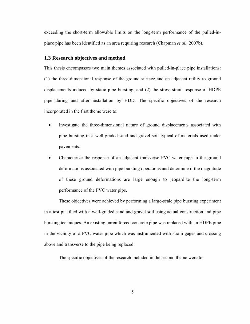
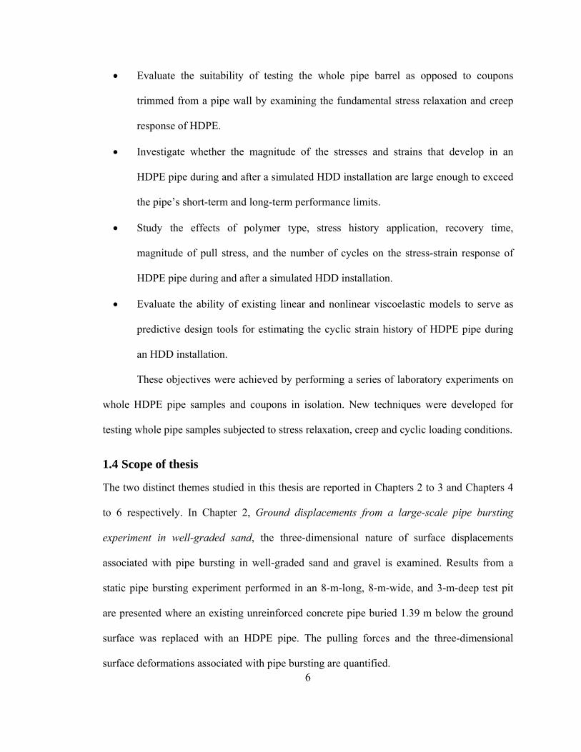
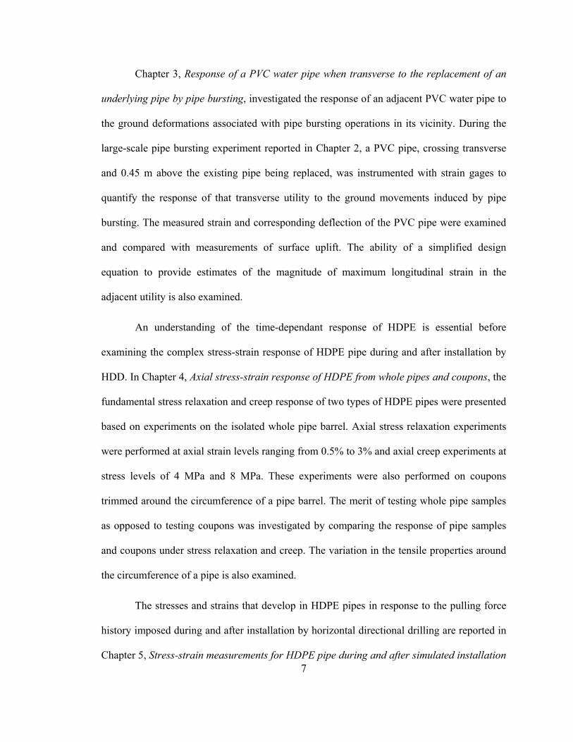
1.3 Research objectives and method......................................................................................5 1.4 Scope of thesis .................................................................................................................6 1.5 Format of thesis ...............................................................................................................8 1.6 References .......................................................................................................................9

Chapter 2 Ground displacements from a large-scale pipe bursting experiment in well-graded sand ............................................................................................................................13

2.1 Introduction ...................................................................................................................13 2.2 Experimental Details .....................................................................................................14

2.2.1 Test Pit ....................................................................................................................14 2.2.2 Materials .................................................................................................................15 2.2.3 Pipe Bursting Process .............................................................................................16 2.2.4 Instrumentation .......................................................................................................16

2.3 Results ...........................................................................................................................17 2.3.1 Pulling Force...........................................................................................................17 2.3.2 Vertical Surface Displacements..............................................................................18 2.3.3 Transverse and axial surface displacements ...........................................................20

2.4 Conclusions ...................................................................................................................23 2.5 References .....................................................................................................................24

Chapter 3 Response of a PVC water pipe when transverse to the replacement of an underlying pipe by pipe bursting .........................................................................................43

3.1 Introduction ...................................................................................................................43 3.2 Experimental details ......................................................................................................44

3.2.1 Test Pit ....................................................................................................................44 3.2.2 Materials .................................................................................................................45 3.2.3 Instrumentation .......................................................................................................46 3.2.4 Method....................................................................................................................47

3.3 Results ...........................................................................................................................47 3.3.1 Longitudinal strains in the PVC pipe......................................................................47

vii

3.3.2 PVC pipe and surface displacements......................................................................48 3.3.3 Circumferential strains in the PVC pipe .................................................................51

3.4 Simplified analysis ........................................................................................................52 3.5 Conclusions ...................................................................................................................54 3.6 References .....................................................................................................................56

Chapter 4 Axial stress-strain response of HDPE from whole pipe samples and coupons.................................................................................................................................................72

4.1 Introduction ...................................................................................................................72 4.2 Details of experiments using pipe samples....................................................................73

4.2.1 Pipe samples ...........................................................................................................73 4.2.2 Stress relaxation experiments .................................................................................74

4.2.2.1 Apparatus and instrumentation ........................................................................74 4.2.2.2 Method .............................................................................................................74

4.2.3 Creep experiments ..................................................................................................76 4.2.3.1 Apparatus and instrumentation ........................................................................76 4.2.3.2 Method .............................................................................................................77

4.3 Details of experiments using coupons ...........................................................................77 4.3.1 Pipe coupons ...........................................................................................................77 4.3.2 Constitutive testing of pipe coupons.......................................................................77

4.3.2.1 Apparatus and instrumentation ........................................................................77 4.3.2.2 Method .............................................................................................................78

4.4 Tests conducted .............................................................................................................78 4.5 Results ...........................................................................................................................79

4.5.1 Stress relaxation......................................................................................................79 4.5.2 Creep.......................................................................................................................81 4.5.3 Strain controlled load path......................................................................................81 4.5.4 Experimental repeatability ......................................................................................83

4.6 Discussion......................................................................................................................83 4.7 Conclusions ...................................................................................................................85 4.8 References .....................................................................................................................86

Chapter 5 Stress-strain measurements for HDPE pipe during and after simulated installation by horizontal directional drilling ...................................................................106

5.1 Introduction .................................................................................................................106 5.2 Experimental details ....................................................................................................107

5.2.1 Pipe samples .........................................................................................................107 5.2.2 Simulation sequence .............................................................................................108 5.2.3 Test method and instrumentation..........................................................................109 5.2.4 Idealized stress history..........................................................................................110 5.2.5 Tests conducted.....................................................................................................111

5.3 Results .........................................................................................................................111 5.3.1 Typical results for PE1 .........................................................................................111 5.3.2 Experimental repeatability ....................................................................................113 5.3.3 Effect of polymer type ..........................................................................................114 5.3.4 Effect of stress increments ....................................................................................114 5.3.5 Effect of recovery time .........................................................................................115

viii

5.3.6 Effect of maximum stress .....................................................................................116 5.3.7 Effect of number of cycles....................................................................................117

5.4 Discussion....................................................................................................................117 5.5 Conclusions .................................................................................................................119 5.6 References ...................................................................................................................121

Chapter 6 Effectiveness of viscoelastic models for prediction of tensile axial strains during cyclic loading of high-density polyethylene ..........................................................140

6.1 Introduction .................................................................................................................140 6.2 Experimental details ....................................................................................................141

6.2.1 Idealized stress history..........................................................................................142 6.2.2 Tests conducted.....................................................................................................143

6.3 Numerical model details ..............................................................................................143 6.3.1 Existing numerical models....................................................................................143 6.3.2 Model geometry....................................................................................................145

6.4 Results .........................................................................................................................146 6.4.1 Laboratory measurements.....................................................................................146 6.4.2 Numerical model evaluation.................................................................................146

6.5 Discussion....................................................................................................................147 6.5.1 Factors affecting installation strains .....................................................................147 6.5.2 Creep function approximation ..............................................................................149

6.6 Conclusions .................................................................................................................150 6.7 References ...................................................................................................................151

Chapter 7 General discussion.............................................................................................165

7.1 Ground displacements and PVC water pipe response during pipe bursting................165 7.1.1 Ground displacements from a large-scale pipe bursting experiment in well-graded sand ................................................................................................................................165 7.1.2 Response of a PVC water pipe when transverse to the replacement of an underlying pipe by pipe bursting ...................................................................................166

7.2 HDPE pipe response during horizontal directional drilling.........................................167 7.2.1 Axial stress-strain response of HDPE from whole pipes and coupons.................167 7.2.2 Stress-strain measurements for HDPE pipe during and after simulated installation by HDD..........................................................................................................................168 7.2.3 Effectiveness of viscoelastic models for prediction of tensile axial strains during cyclic loading of HDPE .................................................................................................169

7.3 References ...................................................................................................................170 Chapter 8 Conclusions and recommendations .................................................................171

8.1 Ground displacements and PVC water pipe response during pipe bursting................171 8.1.1 Ground displacements from a large-scale pipe bursting experiment in well-graded sand ................................................................................................................................171 8.1.2 Response of a PVC water pipe when transverse to the replacement of an underlying pipe by pipe bursting ...................................................................................172

8.2 HDPE pipe response during horizontal directional drilling.........................................172 8.2.1 Axial stress-strain response of HDPE from whole pipes and coupons.................173

ix

8.2.2 Stress-strain measurements for HDPE pipe during and after simulated installation by HDD..........................................................................................................................173 8.2.3 Effectiveness of viscoelastic models for prediction of tensile axial strains during cyclic loading of HDPE .................................................................................................174

8.3 Applicability, limitations, and future work..................................................................174 8.3.1 Ground displacements and PVC water pipe response during pipe bursting .........174 8.3.2 HDPE pipe response during horizontal directional drilling..................................175

8.4 References ...................................................................................................................176 Appendix A Procedure used to determine the accuracy of displacement measurements obtained from digital cameras............................................................................................177 Appendix B Surface scratches on an HDPE pipe installed by pipe bursting.................185

B.1 Introduction.................................................................................................................185 B.2 Experimental details....................................................................................................186 B.3 Results.........................................................................................................................186 B.4 Conclusions and recommendations.............................................................................187 B.5 References...................................................................................................................187

Appendix C Procedure used for determining horizontal ground surface strain from measurements of horizontal surface displacements .........................................................192 Appendix D Procedure used for determining the vertical displacement of the PVC pipe from its curvature................................................................................................................196 Appendix E Determination of the pipe sample gage length.............................................202

E.1 Introduction .................................................................................................................202 E.2 Experimental details....................................................................................................202 E.3 Results and conclusions ..............................................................................................202 E.4 References ...................................................................................................................203

Appendix F Sample Afena input files ................................................................................209

F.1 Sample Afena input files for the linear viscoelastic model .........................................209 F.2 Sample Afena input files for the nonlinear viscoelastic model ...................................215

Appendix G Photographs of experimental details............................................................222

G.1 Ground displacements and PVC water pipe response during pipe bursting...............222 G.2 HDPE pipe response during horizontal directional drilling........................................227

x

List of Tables

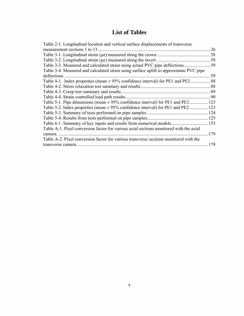
Table 2-1. Longitudinal location and vertical surface displacements of transverse measurement sections 1 to 13..................................................................................................26 Table 3-1. Longitudinal strain (μe) measured along the crown ..............................................58 Table 3-2. Longitudinal strain (μe) measured along the invert ...............................................58 Table 3-3. Measured and calculated strain using actual PVC pipe deflections.......................59 Table 3-4. Measured and calculated strain using surface uplift to approximate PVC pipe deflections ...............................................................................................................................59 Table 4-1. Index properties (mean ± 95% confidence interval) for PE1 and PE2 .................88 Table 4-2. Stress relaxation test summary and results.............................................................88 Table 4-3. Creep test summary and results .............................................................................89 Table 4-4. Strain controlled load path results..........................................................................90 Table 5-1. Pipe dimensions (mean ± 95% confidence interval) for PE1 and PE2 ................123 Table 5-2. Index properties (mean ± 95% confidence interval) for PE1 and PE2 ................123 Table 5-3. Summary of tests performed on pipe samples .....................................................124 Table 5-4. Results from tests performed on pipe samples.....................................................125 Table 6-1. Summary of key inputs and results from numerical models................................153 Table A-1. Pixel conversion factor for various axial sections monitored with the axial camera. ..................................................................................................................................179 Table A-2. Pixel conversion factor for various transverse sections monitored with the transverse camera. .................................................................................................................179

xi

List of Figures

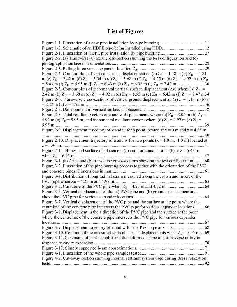
Figure 1-1. Illustration of a new pipe installation by pipe bursting. .......................................11 Figure 1-2. Schematic of an HDPE pipe being installed using HDD......................................12 Figure 2-1. Illustration of HDPE pipe installation by pipe bursting .......................................27 Figure 2-2. (a) Transverse (b) axial cross-section showing the test configuration and (c) photograph of surface instrumentation. ...................................................................................28 Figure 2-3. Pulling force versus expander location ZB............................................................29 Figure 2-4. Contour plots of vertical surface displacement at: (a) ZB = 1.18 m (b) ZB = 1.81 m (c) ZB = 2.42 m (d) ZB = 3.04 m (e) ZB = 3.68 m (f) ZB = 4.25 m (g) ZB = 4.92 m (h) ZB = 5.43 m (i) ZB = 5.95 m (j) ZB = 6.43 m (k) ZB = 6.93 m (l) ZB = 7.47 m.........................30 Figure 2-5. Contour plots of incremental vertical surface displacement (Δv) when: (a) ZB = 2.42 m (b) ZB = 3.68 m (c) ZB = 4.92 m (d) ZB = 5.95 m (e) ZB = 6.43 m (f) ZB = 7.47 m34 Figure 2-6. Transverse cross-sections of vertical ground displacement at: (a) z = 1.18 m (b) z = 2.42 m (c) z = 4.92 m. ..........................................................................................................36 Figure 2-7. Development of vertical surface displacements ...................................................38 Figure 2-8. Total resultant vectors of u and w displacements when: (a) ZB = 3.04 m (b) ZB = 4.92 m (c) ZB = 5.95 m, and incremental resultant vectors when: (d) ZB = 4.92 m (e) ZB = 5.95 m. .....................................................................................................................................39 Figure 2-9. Displacement trajectory of v and w for a point located at x = 0 m and z = 4.88 m..................................................................................................................................................40 Figure 2-10. Displacement trajectory of u and w for two points (x = 1.0 m, -1.0 m) located at z = 3.96 m. ...............................................................................................................................41 Figure 2-11. Horizontal surface displacement (a) and horizontal strains (b) at z = 6.43 m when ZB = 6.93 m....................................................................................................................42 Figure 3-1. (a) Axial and (b) transverse cross-sections showing the test configuration..........60 Figure 3-2. Illustration of the pipe bursting process together with the orientation of the PVC and concrete pipes. Dimensions in mm...................................................................................61 Figure 3-4. Distribution of longitudinal strain measured along the crown and invert of the PVC pipe when ZB = 4.25 m and 4.92 m. ...............................................................................63 Figure 3-5. Curvature of the PVC pipe when ZB = 4.25 m and 4.92 m. .................................64 Figure 3-6. Vertical displacement of the (a) PVC pipe and (b) ground surface measured above the PVC pipe for various expander locations................................................................65 Figure 3-7. Vertical displacement of the PVC pipe and the surface at the point where the centreline of the concrete pipe intersects the PVC pipe for various expander locations.........66 Figure 3-8. Displacement in the z direction of the PVC pipe and the surface at the point where the centreline of the concrete pipe intersects the PVC pipe for various expander locations...................................................................................................................................67 Figure 3-9. Displacement trajectory of v and w for the PVC pipe at x = 0.............................68 Figure 3-10. Contours of the measured vertical surface displacements when ZB = 5.95 m....69 Figure 3-11. Schematic of surface uplift and the deformed shape of a transverse utility in response to cavity expansion. ..................................................................................................70 Figure 3-12. Simply supported beam approximations.............................................................71 Figure 4-1. Illustration of the whole pipe samples tested........................................................91 Figure 4-2. Cut-away section showing internal restraint system used during stress relaxation tests ..........................................................................................................................................92

xii

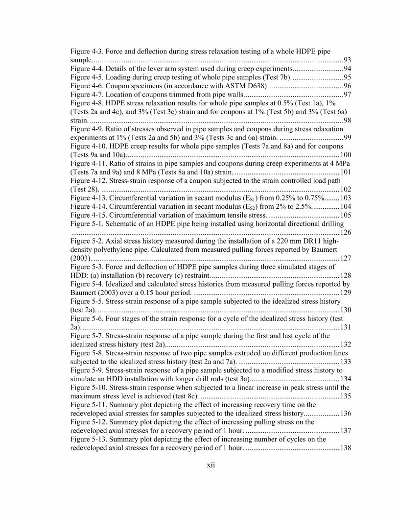
Figure 4-3. Force and deflection during stress relaxation testing of a whole HDPE pipe sample......................................................................................................................................93 Figure 4-4. Details of the lever arm system used during creep experiments...........................94 Figure 4-5. Loading during creep testing of whole pipe samples (Test 7b). ...........................95 Figure 4-6. Coupon specimens (in accordance with ASTM D638) ........................................96 Figure 4-7. Location of coupons trimmed from pipe walls.....................................................97 Figure 4-8. HDPE stress relaxation results for whole pipe samples at 0.5% (Test 1a), 1% (Tests 2a and 4c), and 3% (Test 3c) strain and for coupons at 1% (Test 5b) and 3% (Test 6a) strain. .......................................................................................................................................98 Figure 4-9. Ratio of stresses observed in pipe samples and coupons during stress relaxation experiments at 1% (Tests 2a and 5b) and 3% (Tests 3c and 6a) strain. ..................................99 Figure 4-10. HDPE creep results for whole pipe samples (Tests 7a and 8a) and for coupons (Tests 9a and 10a)..................................................................................................................100 Figure 4-11. Ratio of strains in pipe samples and coupons during creep experiments at 4 MPa (Tests 7a and 9a) and 8 MPa (Tests 8a and 10a) strain. ........................................................101 Figure 4-12. Stress-strain response of a coupon subjected to the strain controlled load path (Test 28). ...............................................................................................................................102 Figure 4-13. Circumferential variation in secant modulus (ES1) from 0.25% to 0.75%........103 Figure 4-14. Circumferential variation in secant modulus (ES2) from 2% to 2.5%...............104 Figure 4-15. Circumferential variation of maximum tensile stress. ......................................105 Figure 5-1. Schematic of an HDPE pipe being installed using horizontal directional drilling...............................................................................................................................................126 Figure 5-2. Axial stress history measured during the installation of a 220 mm DR11 high-density polyethylene pipe. Calculated from measured pulling forces reported by Baumert (2003). ...................................................................................................................................127 Figure 5-3. Force and deflection of HDPE pipe samples during three simulated stages of HDD: (a) installation (b) recovery (c) restraint. ....................................................................128 Figure 5-4. Idealized and calculated stress histories from measured pulling forces reported by Baumert (2003) over a 0.15 hour period. ..............................................................................129 Figure 5-5. Stress-strain response of a pipe sample subjected to the idealized stress history (test 2a). .................................................................................................................................130 Figure 5-6. Four stages of the strain response for a cycle of the idealized stress history (test 2a). .........................................................................................................................................131 Figure 5-7. Stress-strain response of a pipe sample during the first and last cycle of the idealized stress history (test 2a).............................................................................................132 Figure 5-8. Stress-strain response of two pipe samples extruded on different production lines subjected to the idealized stress history (test 2a and 7a). ......................................................133 Figure 5-9. Stress-strain response of a pipe sample subjected to a modified stress history to simulate an HDD installation with longer drill rods (test 3a)................................................134 Figure 5-10. Stress-strain response when subjected to a linear increase in peak stress until the maximum stress level is achieved (test 8c). ..........................................................................135 Figure 5-11. Summary plot depicting the effect of increasing recovery time on the redeveloped axial stresses for samples subjected to the idealized stress history...................136 Figure 5-12. Summary plot depicting the effect of increasing pulling stress on the redeveloped axial stresses for a recovery period of 1 hour. ..................................................137 Figure 5-13. Summary plot depicting the effect of increasing number of cycles on the redeveloped axial stresses for a recovery period of 1 hour. ..................................................138

xiii

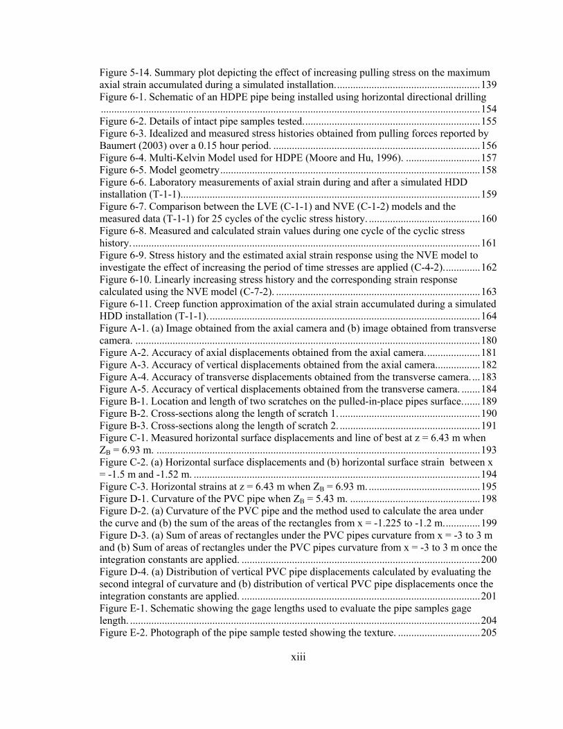
Figure 5-14. Summary plot depicting the effect of increasing pulling stress on the maximum axial strain accumulated during a simulated installation.......................................................139 Figure 6-1. Schematic of an HDPE pipe being installed using horizontal directional drilling...............................................................................................................................................154 Figure 6-2. Details of intact pipe samples tested...................................................................155 Figure 6-3. Idealized and measured stress histories obtained from pulling forces reported by Baumert (2003) over a 0.15 hour period. ..............................................................................156 Figure 6-4. Multi-Kelvin Model used for HDPE (Moore and Hu, 1996). ............................157 Figure 6-5. Model geometry..................................................................................................158 Figure 6-6. Laboratory measurements of axial strain during and after a simulated HDD installation (T-1-1).................................................................................................................159 Figure 6-7. Comparison between the LVE (C-1-1) and NVE (C-1-2) models and the measured data (T-1-1) for 25 cycles of the cyclic stress history. ..........................................160 Figure 6-8. Measured and calculated strain values during one cycle of the cyclic stress history. ...................................................................................................................................161 Figure 6-9. Stress history and the estimated axial strain response using the NVE model to investigate the effect of increasing the period of time stresses are applied (C-4-2)..............162 Figure 6-10. Linearly increasing stress history and the corresponding strain response calculated using the NVE model (C-7-2). .............................................................................163 Figure 6-11. Creep function approximation of the axial strain accumulated during a simulated HDD installation (T-1-1).......................................................................................................164 Figure A-1. (a) Image obtained from the axial camera and (b) image obtained from transverse camera. ..................................................................................................................................180 Figure A-2. Accuracy of axial displacements obtained from the axial camera.....................181 Figure A-3. Accuracy of vertical displacements obtained from the axial camera.................182 Figure A-4. Accuracy of transverse displacements obtained from the transverse camera. ...183 Figure A-5. Accuracy of vertical displacements obtained from the transverse camera. .......184 Figure B-1. Location and length of two scratches on the pulled-in-place pipes surface.......189 Figure B-2. Cross-sections along the length of scratch 1. .....................................................190 Figure B-3. Cross-sections along the length of scratch 2. .....................................................191 Figure C-1. Measured horizontal surface displacements and line of best at z = 6.43 m when ZB = 6.93 m. ..........................................................................................................................193 Figure C-2. (a) Horizontal surface displacements and (b) horizontal surface strain between x = -1.5 m and -1.52 m. ............................................................................................................194 Figure C-3. Horizontal strains at z = 6.43 m when ZB = 6.93 m. ..........................................195 Figure D-1. Curvature of the PVC pipe when ZB = 5.43 m. .................................................198 Figure D-2. (a) Curvature of the PVC pipe and the method used to calculate the area under the curve and (b) the sum of the areas of the rectangles from x = -1.225 to -1.2 m..............199 Figure D-3. (a) Sum of areas of rectangles under the PVC pipes curvature from x = -3 to 3 m and (b) Sum of areas of rectangles under the PVC pipes curvature from x = -3 to 3 m once the integration constants are applied. ..........................................................................................200 Figure D-4. (a) Distribution of vertical PVC pipe displacements calculated by evaluating the second integral of curvature and (b) distribution of vertical PVC pipe displacements once the integration constants are applied. ..........................................................................................201 Figure E-1. Schematic showing the gage lengths used to evaluate the pipe samples gage length. ....................................................................................................................................204 Figure E-2. Photograph of the pipe sample tested showing the texture. ...............................205

xiv

Figure E-3. Strain calculated over various gage lengths compared against the strain calculated using a pipe sample gage extending between the ends of the flanged HDPE fittings...........206 Figure G-1. Backfilling the test pit, showing the 3 m tall retaining wall. .............................222 Figure G-2. Placement of unreinforced concrete pipe...........................................................223 Figure G-3. Detail of geotextile used around concrete pipe at entry and exit portholes. ......223 Figure G-4. Photograph of instrumented PVC pipe prior to burial. ......................................224 Figure G-5. Actuator used to pull the expander. ...................................................................225 Figure G-6. Expander prior to entering test pit. ....................................................................225 Figure G-7. Ground surface instrumentation.........................................................................226 Figure G-8. Photograph of tension crack observed on the ground surface. ..........................226 Figure G-9. Instron loading machine and pipe samples tested..............................................227 Figure G-10. Extensometer and grips used to test coupons. .................................................228

1

Chapter 1

Introduction

1.1 Description of problem

1.1.1 State of existing pipelines

Pipelines provide essential services to our urban centres. With these urban centres continually

growing and expanding, demand on the existing buried services is also increasing. Existing

pipeline systems may be either deteriorated or hydraulically undersized and can contribute to

the pollution of our urban centres (e.g. the overflow of small diameter combined sewer pipes

into basements). Expanding capacity and limiting groundwater inflows through these

deficient pipes is essential to maintain the urban environment and quality of life.

Construction techniques used to install new pipes, without the need for the extensive surface

disruptions associated with traditional cut-and-cover construction, include static pipe bursting

and horizontal directional drilling (HDD).

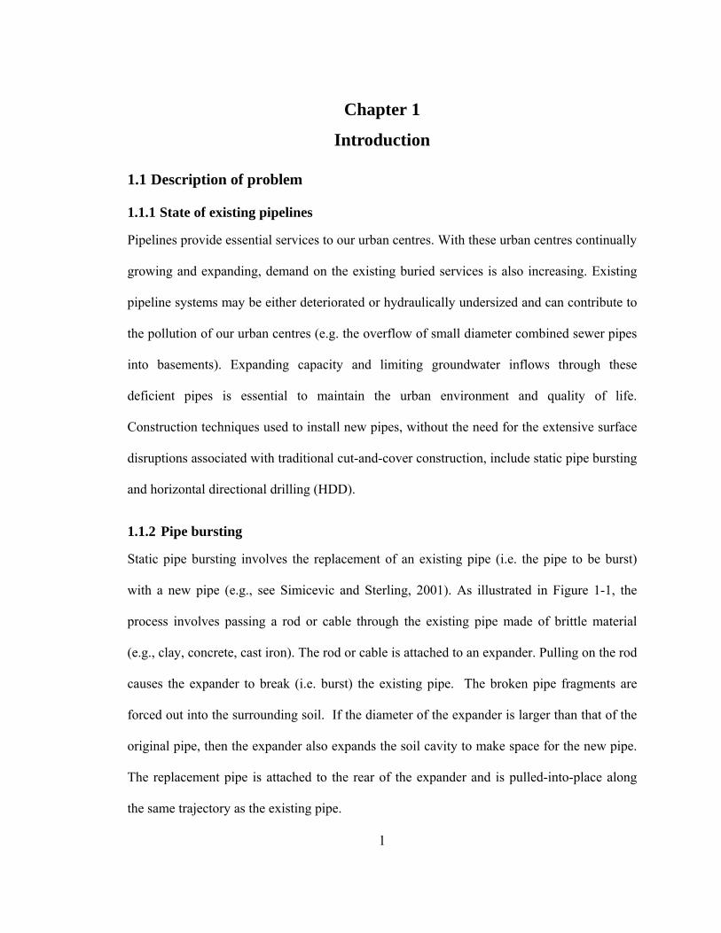
1.1.2 Pipe bursting

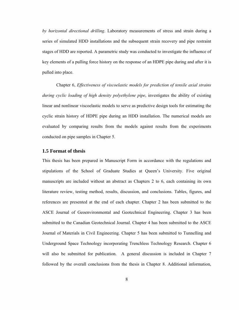
Static pipe bursting involves the replacement of an existing pipe (i.e. the pipe to be burst)

with a new pipe (e.g., see Simicevic and Sterling, 2001). As illustrated in Figure 1-1, the

process involves passing a rod or cable through the existing pipe made of brittle material

(e.g., clay, concrete, cast iron). The rod or cable is attached to an expander. Pulling on the rod

causes the expander to break (i.e. burst) the existing pipe. The broken pipe fragments are

forced out into the surrounding soil. If the diameter of the expander is larger than that of the

original pipe, then the expander also expands the soil cavity to make space for the new pipe.

The replacement pipe is attached to the rear of the expander and is pulled-into-place along

the same trajectory as the existing pipe.

2

Of particular interest is the nature and magnitude of the ground deformations that are

generated during pipe bursting. Further, there is a potential concern that if pipe bursting

operations are conducted in the vicinity of an adjacent pipe, these ground deformations may

potentially damage the pipe. To quantify the three-dimensional nature of surface and sub-

surface ground displacements, physical pipe bursting experiments in poorly-graded sand

were conducted by Rogers and Chapman (1995) within a 1.5-m-long, 1-m-wide and 1.5-m-

deep glass-sided tank, and by Lapos (2004) in a 2-m-long, 2-m-wide and 1.6-m-deep test cell.

These studies contributed to the understanding of the mechanics of pipe bursting; however,

the small scale of the experiments means that the results may have been influenced by

boundary effects. Results from field pipe bursting trials performed by Atalah (1998) in four

different soil conditions (clay, sand, silt, and a clay-gravel mixture) concluded that ground

displacements induced by pipe bursting are dependent on the degree of upsizing, type and

degree of compaction of the soil, and the depth of cover above the pipe being replaced.

There have been limited experimental studies that investigate the response of an

adjacent pipe, in particular a polyvinyl chloride (PVC) water pipe, to ground displacements

caused by pipe bursting. Atalah (1998) monitored pressure in transverse PVC pipes in the

vicinity of pipe bursting operations. During one particular test in sand, the polyvinyl chloride

pipe crossing 300 mm above the clay pipe being upsized by 50% lost internal pressure,

suggesting the pipe was damaged. For cases when internal pressure was maintained, the

short-term capacity of the pipe may not have been exceeded; however, the strains that

developed in these pipes are of interest to determine if potential long-term performance limits

were exceeded. Furthermore, the specific characteristics of the adjacent pipe deformation

were not developed in detail.

3

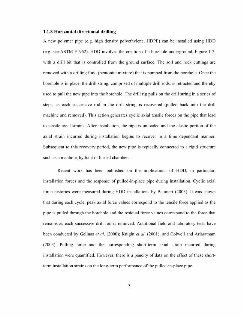
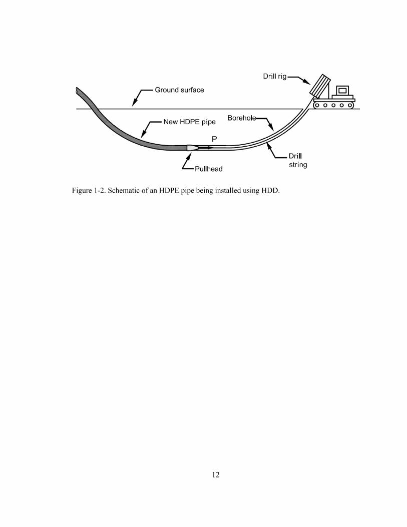
1.1.3 Horizontal directional drilling

A new polymer pipe (e.g. high density polyethylene, HDPE) can be installed using HDD

(e.g. see ASTM F1962). HDD involves the creation of a borehole underground, Figure 1-2,

with a drill bit that is controlled from the ground surface. The soil and rock cuttings are

removed with a drilling fluid (bentonite mixture) that is pumped from the borehole. Once the

borehole is in place, the drill string, comprised of multiple drill rods, is retracted and thereby

used to pull the new pipe into the borehole. The drill rig pulls on the drill string in a series of

steps, as each successive rod in the drill string is recovered (pulled back into the drill

machine and removed). This action generates cyclic axial tensile forces on the pipe that lead

to tensile axial strains. After installation, the pipe is unloaded and the elastic portion of the

axial strain incurred during installation begins to recover in a time dependant manner.

Subsequent to this recovery period, the new pipe is typically connected to a rigid structure

such as a manhole, hydrant or buried chamber.

Recent work has been published on the implications of HDD, in particular,

installation forces and the response of pulled-in-place pipe during installation. Cyclic axial

force histories were measured during HDD installations by Baumert (2003). It was shown

that during each cycle, peak axial force values correspond to the tensile force applied as the

pipe is pulled through the borehole and the residual force values correspond to the force that

remains as each successive drill rod is removed. Additional field and laboratory tests have

been conducted by Gelinas et al. (2000); Knight et al. (2001); and Colwell and Ariaratnam

(2003). Pulling force and the corresponding short-term axial strain incurred during

installation were quantified. However, there is a paucity of data on the effect of these short-

term installation strains on the long-term performance of the pulled-in-place pipe.

4

1.2 Current state of practice

1.2.1 Pipe bursting

Procedures have been developed for estimating the magnitude of ground displacements as a

result of the cavity expansion during pipe bursting (Nkemitag and Moore, 2006). Now, while

there has been extensive research into the ground displacements associated with pipe

bursting, there is still a need for further research in this area, particularly in stiff and dense

soils (Chapman et al., 2007a).

When pipe bursting in the vicinity of an adjacent utility, the distance between the

adjacent utility and pipe being replaced must be checked to avoid damage that may occur due

to ground displacements. Proximity charts are available to identify whether or not the

integrity of a grey cast iron pipe would be in jeopardy if pipe bursting operations were

performed in its vicinity (Transco, 1997); however, these charts have been developed on the

basis of very limited field studies and further research is required to improve the

understanding of potential damage to adjacent utilities (Chapman et al., 2007a).

1.2.2 Horizontal directional drilling

In terms of the durability of pulled-in-place pipe during HDD, pulling force equations have

been suggested to estimate the maximum pulling force for a particular installation, Baumert

and Allouche (2002). This estimated pulling force is compared to allowable limits to ensure

the tensile axial stresses do not exceed the short-term yield capacity of the pipe (ASTM

F1804; AWWA M55). However, a more detailed investigation of the axial stresses and

strains imposed during and after an HDD installation is required to quantify the effect of

cyclic loading on the maximum axial strain that develops during installation, and the long

term performance of HDPE pipe after it is pulled-in-place. In particular, the influence of

5

exceeding the short-term allowable limits on the long-term performance of the pulled-in-

place pipe has been identified as an area requiring research (Chapman et al., 2007b).

1.3 Research objectives and method

This thesis encompasses two main themes associated with pulled-in-place pipe installations:

(1) the three-dimensional response of the ground surface and an adjacent utility to ground

displacements induced by static pipe bursting, and (2) the stress-strain response of HDPE

pipe during and after installation by HDD. The specific objectives of the research

incorporated in the first theme were to:

• Investigate the three-dimensional nature of ground displacements associated with

pipe bursting in a well-graded sand and gravel soil typical of materials used under

pavements.

• Characterize the response of an adjacent transverse PVC water pipe to the ground

deformations associated with pipe bursting operations and determine if the magnitude

of these ground deformations are large enough to jeopardize the long-term

performance of the PVC water pipe.

These objectives were achieved by performing a large-scale pipe bursting experiment

in a test pit filled with a well-graded sand and gravel soil using actual construction and pipe

bursting techniques. An existing unreinforced concrete pipe was replaced with an HDPE pipe

in the vicinity of a PVC water pipe which was instrumented with strain gages and crossing

above and transverse to the pipe being replaced.

The specific objectives of the research included in the second theme were to:

6

• Evaluate the suitability of testing the whole pipe barrel as opposed to coupons

trimmed from a pipe wall by examining the fundamental stress relaxation and creep

response of HDPE.

• Investigate whether the magnitude of the stresses and strains that develop in an

HDPE pipe during and after a simulated HDD installation are large enough to exceed

the pipe’s short-term and long-term performance limits.

• Study the effects of polymer type, stress history application, recovery time,

magnitude of pull stress, and the number of cycles on the stress-strain response of

HDPE pipe during and after a simulated HDD installation.

• Evaluate the ability of existing linear and nonlinear viscoelastic models to serve as

predictive design tools for estimating the cyclic strain history of HDPE pipe during

an HDD installation.

These objectives were achieved by performing a series of laboratory experiments on

whole HDPE pipe samples and coupons in isolation. New techniques were developed for

testing whole pipe samples subjected to stress relaxation, creep and cyclic loading conditions.

1.4 Scope of thesis

The two distinct themes studied in this thesis are reported in Chapters 2 to 3 and Chapters 4

to 6 respectively. In Chapter 2, Ground displacements from a large-scale pipe bursting

experiment in well-graded sand, the three-dimensional nature of surface displacements

associated with pipe bursting in well-graded sand and gravel is examined. Results from a

static pipe bursting experiment performed in an 8-m-long, 8-m-wide, and 3-m-deep test pit

are presented where an existing unreinforced concrete pipe buried 1.39 m below the ground

surface was replaced with an HDPE pipe. The pulling forces and the three-dimensional

surface deformations associated with pipe bursting are quantified.

7

Chapter 3, Response of a PVC water pipe when transverse to the replacement of an

underlying pipe by pipe bursting, investigated the response of an adjacent PVC water pipe to

the ground deformations associated with pipe bursting operations in its vicinity. During the

large-scale pipe bursting experiment reported in Chapter 2, a PVC pipe, crossing transverse

and 0.45 m above the existing pipe being replaced, was instrumented with strain gages to

quantify the response of that transverse utility to the ground movements induced by pipe

bursting. The measured strain and corresponding deflection of the PVC pipe were examined

and compared with measurements of surface uplift. The ability of a simplified design

equation to provide estimates of the magnitude of maximum longitudinal strain in the

adjacent utility is also examined.

An understanding of the time-dependant response of HDPE is essential before

examining the complex stress-strain response of HDPE pipe during and after installation by

HDD. In Chapter 4, Axial stress-strain response of HDPE from whole pipes and coupons, the

fundamental stress relaxation and creep response of two types of HDPE pipes were presented

based on experiments on the isolated whole pipe barrel. Axial stress relaxation experiments

were performed at axial strain levels ranging from 0.5% to 3% and axial creep experiments at

stress levels of 4 MPa and 8 MPa. These experiments were also performed on coupons

trimmed around the circumference of a pipe barrel. The merit of testing whole pipe samples

as opposed to testing coupons was investigated by comparing the response of pipe samples

and coupons under stress relaxation and creep. The variation in the tensile properties around

the circumference of a pipe is also examined.

The stresses and strains that develop in HDPE pipes in response to the pulling force

history imposed during and after installation by horizontal directional drilling are reported in

Chapter 5, Stress-strain measurements for HDPE pipe during and after simulated installation

8

by horizontal directional drilling. Laboratory measurements of stress and strain during a

series of simulated HDD installations and the subsequent strain recovery and pipe restraint

stages of HDD are reported. A parametric study was conducted to investigate the influence of

key elements of a pulling force history on the response of an HDPE pipe during and after it is

pulled into place.

Chapter 6, Effectiveness of viscoelastic models for prediction of tensile axial strains

during cyclic loading of high density polyethylene pipe, investigates the ability of existing

linear and nonlinear viscoelastic models to serve as predictive design tools for estimating the

cyclic strain history of HDPE pipe during an HDD installation. The numerical models are

evaluated by comparing results from the models against results from the experiments

conducted on pipe samples in Chapter 5.

1.5 Format of thesis

This thesis has been prepared in Manuscript Form in accordance with the regulations and

stipulations of the School of Graduate Studies at Queen’s University. Five original

manuscripts are included without an abstract as Chapters 2 to 6, each containing its own

literature review, testing method, results, discussion, and conclusions. Tables, figures, and

references are presented at the end of each chapter. Chapter 2 has been submitted to the

ASCE Journal of Geoenvironmental and Geotechnical Engineering. Chapter 3 has been

submitted to the Canadian Geotechnical Journal. Chapter 4 has been submitted to the ASCE

Journal of Materials in Civil Engineering. Chapter 5 has been submitted to Tunnelling and

Underground Space Technology incorporating Trenchless Technology Research. Chapter 6

will also be submitted for publication. A general discussion is included in Chapter 7

followed by the overall conclusions from the thesis in Chapter 8. Additional information,

9

including photographs of experimental details, is provided in the appendices. The

International System of measurements was used consistently throughout this thesis.

1.6 References

ASTM F 1804-08. Standard Practice for Determining Allowable Tensile Load for Polyethylene (PE) Gas Pipe During Pull-In Installation. ASTM International, West Conshohocken, PA.

ASTM F 1962-05 Standard Guide for Use of Maxi-Horizontal Directional Drilling for Placement of Polyethylene Pipe or Conduit Under Obstacles, Including River Crossings. ASTM International, West Conshohocken, PA.

AWWA M55. PE Pipe – Design and Installation (M55). American Water Works Association, Denver, COL.

Atalah, A. 1998. The effect of pipe bursting on near by utilities, pavement and structures. Technical Report: TT 98-01. Trenchless Technology Center. Louisiana Tech University.

Baumert, M. E. and Allouche, E. N. 2002. Methods for estimating pipe pullback loads for horizontal directional drilling crossings, Journal of Infrastructure Systems, ASCE, 8(1): 12-19.

Baumert, M.E. 2003. Experimental investigation of pulling loads and mud pressures during horizontal directional drilling installations. PhD Thesis, The University of Western Ontario, London, Ontario.

Chapman, D.N., Ng, P.C.F. and Karri, R. 2007a. Research needs for on-line pipeline replacement techniques. Tunnelling and Underground Space Technology, 22(5), 503- 514.

Chapman, D.N., Rogers, C.D.F., Burd, H.J., Norris, P.M., and Milligan, G.W.E. 2007b. Research needs for new construction using trenchless technologies. Tunnelling and Underground Space Technology, 22(5), 491-502.

Colwell, D.A.F. and Ariaratnam, S.T. 2003. Evaluation of high-density polyethylene pipe installed using horizontal directional drilling. Journal of Construction Engineering and Management, Vol. 129, No.1: 47-55.

Gelinas, M., Polak, M.A. and McKim, R. 2000. Field tests on HDPE pipes installed using horizontal direction drilling. Journal of Infrastructure Systems, Vol. 6, No. 4: 130-137

Knight, M.A., Duyvestyn, G.M. and Polak, M.A. 2001. Horizontal directional drilling research program – University of Waterloo. Proceeding of Underground Infrastructure Research Conferecne, June 11 to 13 2001. Kitchener, Ontario.

10

Lapos, B.M. 2004. Laboratory study of static pipe bursting three-dimensional ground displacements and pull force during installation, and subsequent response of HDPE replacement pipes under surcharge loading. M.Sc. Thesis, Dept. of Civil Engineering, Queen’s University, Kingston, Ont.

Nkemitag, M. and Moore, I.D. 2006. Rational guidelines for expected ground disturbance during static pipe bursting through sand, Paper E-2-01, North American No-Dig 2006, Nashville, TN, 9pp.

Rogers, C.D.F., and Chapman, D.N. 1995. An experimental study of pipe bursting in sand. Proc., Inst. Civ. Eng., London, 113(1), 38-50.

Simicevic, J., and Sterling, R.L. 2001. Guidelines for pipe bursting. TTC technical report #2001.02, U.S. Army Corps of Engineers.

Transco. 1997. Damage Control Procedure for Pipeline Construction Involving Pipe Splitting. Transco BG Plc (now part of National Grid Transco), Technical Publication No. 4558/3250.

11

Figure 1-1. Illustration of a new pipe installation by pipe bursting.

12

Figure 1-2. Schematic of an HDPE pipe being installed using HDD.

13

Chapter 2

Ground displacements from a large-scale pipe bursting experiment

in well-graded sand

2.1 Introduction

Static pipe bursting is a construction technique that involves the replacement of an existing

pipe (i.e. the pipe to be burst) that may be either deteriorated or hydraulically undersized

(e.g., see Simicevic and Sterling 2001). This process is performed without the need for the

extensive surface disruptions of traditional cut-and-cover construction. As illustrated in

Figure 2-1, the process involves passing a rod or cable through the existing pipe made of

brittle material (e.g., clay, concrete, cast iron). The rod or cable is attached to an expander.

Pulling on the rod causes the expander to break (i.e. burst) the existing pipe. The broken pipe

fragments are forced into the surrounding soil. If the diameter of the expander is larger than

that of the original pipe, then the expander also expands the soil cavity for the new pipe. The

replacement pipe is attached to the rear of the expander and is pulled-into-place along the

same trajectory as the existing pipe. Of specific interest in this work is the force required to

conduct the pipe bursting operation and the resulting surface displacements.

Physical experiments on pipe bursting in poorly-graded sand have been conducted by

Rogers and Chapman (1995) within a 1.5-m-long, 1-m-wide and 1.5-m-deep glass-sided tank

and by Lapos (2004) in a 2-m-long, 2-m-wide and 1.6-m-deep test cell. The three-

dimensional nature of surface and subsurface ground displacements were quantified. The

results of these studies may have been influenced by boundary effects and the impacts of

these effects could be assessed with numerical modelling. However, when extending this

14

work to consider coarser-grained and/or well-graded materials it was evident that even the

larger apparatus of Lapos (2004) would have excessive boundary effects.

It is the objective of this chapter to quantify ground displacements associated with

pipe bursting in a well-graded sand and gravel soil typical of materials used under

pavements. A large-scale pipe bursting experiment was performed in an 8-m-long, 8-m-wide,

and 3-m-deep test pit using actual construction and pipe bursting techniques. The pulling

forces and ground deformations associated with pipe bursting are presented.

2.2 Experimental Details

2.2.1 Test Pit

This static pipe bursting experiment was carried out in an 8-m-long, 8-m-wide, and 3-m-deep

test pit. A schematic of the experiment is provided in Figure 2-2. The boundary conditions

consisted of three rigid concrete walls: (a) East wall (z = 8 m, x= -4 m to 4 m); (b) North wall

(x = -4 m, z = 0 m to 8 m); and (c) South wall (x = 4 m, z = 0 m to 8 m). The West wall (z =

0 m, x= -4 m to 4 m) was a removable stiff concrete wall (i.e. the pit is actually 16 m long).

The base of the West wall was anchored to the concrete floor and was buttressed on the West

side with granular fill to reduce the horizontal displacement of the top of the wall to less than

10 mm. The concrete walls were formed smooth and no effort was made to further reduce

friction. Given the size of the test pit, the imposed restraint from boundary friction was not

expected to affect the ground displacements over most of the pit; the potential impact of the

boundary roughness on the measured results is examined later in this chapter. Portholes are

located on the East and West walls at x = 0 m to allow access for the pulling rods, expander,

and replacement pipe. The replacement pipe was pulled into place through the porthole in

the West wall toward the East wall as illustrated in Figure 2-2b.

15

2.2.2 Materials

The pit was filled with a well-graded sand and gravel having a coefficient of uniformity (Cu)

of 20 and a coefficient of curvature (Cc) and 0.5. The material has a standard Proctor

maximum dry density of 2.25 g/cm3, an optimum water content of 5%, and a maximum and

minimum dry density of 2.46 g/cm3 and 1.87 g/cm3, respectively. The soil was placed in the

pit in 300-mm-thick lifts and compacted using a vibrating plate tamper (Wacker 1550 with an

operating mass of 88 kg and a maximum centrifugal force of 15 kN). The average as-placed

dry density and water content was 2.13 ± 0.01 g/cm3 and 4.6 ± 0.9 %, respectively (where ±

is one standard deviation). At this density and water content, a peak friction angle between

54-56° was obtained from large-scale triaxial testing for the range of confining stresses

expected in the pipe bursting experiment (Scott et al., 1977).

The existing pipe was a new unreinforced concrete pipe with an outside diameter

(OD) of 229 mm and an average wall thickness of 38 mm. The high-density polyethylene

(HDPE) replacement pipe had an OD of 168 mm and an average wall thickness of 11 mm. To

investigate the influence of pipe bursting on an adjacent utility, a polyvinyl chloride (PVC)

pipe with an OD of 122 mm and an average wall thickness of 7 mm was buried above and

transverse to the existing pipe. The locations of the three pipes used in the experiment are

shown in Figure 2-2b. There was 1385 mm of cover above the existing pipe and 815 mm of

cover above the adjacent utility (crown to the surface). The vertical distance between the

invert of the adjacent utility and the crown of the existing pipe was 450 mm. At the portholes,

300 mm of the concrete pipe was wrapped in a geotextile to prevent the sand and gravel soil

from flowing through the gap between the concrete pipe and the porthole.

16

2.2.3 Pipe Bursting Process

A hydraulic actuator (mounted behind the East porthole) was used to pull the expander

through the existing pipe and pull the replacement pipe into place. The particular expander

used (Figure 2-1) had a maximum diameter of 202 mm. The expander was attached to 32-

mm-diameter, 300-mm-long steel rods that were connected to the actuator. A swivel was

used to allow for free rotation of the expander. Pulling was performed at a controlled

displacement rate of 100 mm/min. The expander entered the pit at z = 0 m and x = 0 m as the

8-m-long replacement pipe was strung out in the adjacent partially empty pit. Pulling was

paused for 15–20 minutes at thirteen transverse sections located along the length of the

existing pipe (S1–S13, shown in Figure 2-2b with their locations given in Table 2-1) to

measure the ground displacements when the expander was directly beneath each section.

2.2.4 Instrumentation

The pulling force, ground deformations, and strains of the adjacent utility were monitored

during the pipe bursting process. A load cell was used to measure pulling force during the

experiment to an accuracy of ± 1 N. It was located between the actuator and pulling rods.

Three-dimensional surface displacements (u, v and w in the x, y and z directions,

respectively, as defined in Figure 2-2) were measured using 349 targets tracked with digital

cameras and 30 prisms electronically tracked with a total station. A photograph of the surface

instrumentation between S4 and S9 is given in Figure 2-2c. Images obtained from the

cameras were analyzed using the image-based deformation software, geoPIV (White et al.,

2003). The accuracy of the displacements obtained with the cameras and the total station are

± 0.1 mm and ± 0.3 mm, respectively. Details of the procedure used to determine the

accuracy of the displacements obtained with the cameras are provided in Appendix A.

17

2.3 Results

2.3.1 Pulling Force

The measured pulling force (P) is shown for a given expander location (ZB) in Figure 2-3.

The maximum pulling force of 209 kN was measured when the expander was at ZB = 3.65 m.

The results also show zones of sudden increases in measured pulling force between 20–50 kN

followed by subsequent decreases. Since the concrete pipe was wrapped in a geotextile, the

data close to the entry and exit of the expander from the pit was neglected, giving a mean

pulling force of 149 ± 0.3 kN (i.e., for 1.0 m ≤ ZB ≤ 7.0 m).

The measured pulling force can be attributed to three components: (1) the axial force

required on the expander to break the existing concrete pipe, (2) the axial force required on

the expander to expand the soil cavity radially outwards and move the expander forwards,

and (3) the axial force mobilized because of friction between the HDPE replacement pipe and

the broken concrete pipe. In a separate experiment, an axial force of 5 kN was required to

burst an unconfined specimen of the concrete pipe with the expander. The force required to

break the existing concrete pipe when buried in soil would be expected to be even larger to

overcome the compressive stresses in the concrete pipe (from the weight of the surrounding

soil) and possibly from an increase in the tensile strength of the concrete pipe from soil

confining pressures. Based on the results in Figure 2-3, the sudden zones of increasing and

then decreasing force are attributed to crack initiation and propagation in the existing

concrete pipe and thereby approximately 20–50 kN of the measured pulling force is

attributed to the breaking of the existing concrete pipe. At the completion of the pipe

bursting experiment, after the expander has exited the porthole, an axial force of only 2 kN

was required to pull the replacement pipe further. This represents the frictional force that

acted along the 8-m-long HDPE pipe. Thus the largest component of the measured pulling

18

force is that required to expand the soil cavity and move the expander forward

(approximately 100–130 kN).

Once installed, the replacement HDPE pipe was exhumed to quantify the scratches

incurred on the pipe’s surface from interacting with the broken fragments of the unreinforced

concrete pipe. These results are reported in Appendix B.

2.3.2 Vertical Surface Displacements

Contours of the measured vertical surface displacements (v) are given in Figure 2-4 for

different stages of the experiment as the expander progressed through the existing concrete

pipe. Upward vertical displacements are taken as positive. Figure 2-4a and Figure 2-4b

show the early development of the surface response to pipe bursting. Here, the maximum

vertical displacement is less than 3.5 mm. Displacements extend approximately 1.2 m in

advance of the expander and 1.8 m on either side of the centre line, as defined by the 0.5 mm

contour. As the expander advances further into the soil (Figure 2-4c-g), the vertical

displacements increase to a maximum of 6 mm at section S9 (Figure 2-4h), while

displacements extend between 1.6 to 1.8 m in advance of the expander and no more than 2 m

on either side of the centerline (neglecting small deformations that could not be recorded by

the instrumentation). In fact, the maximum width of the zone of influence on the surface at

any point during the test was no greater than 4 m (i.e. -2 < x < 2 m). Thus the lateral

boundaries of the 8-m-wide pit were sufficiently far enough away so as not to impact the

measured ground displacements. However, as the expander approaches the rigid boundary at

z = 8 m, it appears that the measured ground displacements located at and beyond z = 5.95 m

have been influenced by the boundary as the leading edge of the ground response in Figure 2-

4i-l begins to interact with the wall.

19

To further investigate the effects of the end boundary, contours of incremental

vertical surface displacements (Δv) from one pull to another are given in Figure 2-5. For

example, the results in Figure 2-5a were obtained by subtracting the vertical displacements

when the expander was at S3 from those when it was at S4. Based on the shape and

magnitude of the Δv response, surface displacements up to z = 5.95 m were not influenced by

the rigid end boundary. The magnitude and circular shape, as defined by the 0.5 mm contour,

of Δv remains consistent until the expander has moved beyond z = 5.95 m (Figure 2-5a-d). In

Figure 2-5e the incremental response is close to but not intersecting the wall, however, it is

no longer circular in shape and the magnitude of Δv decreases. As the expander further

approaches the rigid boundary the incremental response intersects the wall (Figure 2-5f).

Here, the shape is smaller in the z-direction and larger in the x-direction compared to the

more circular shape of the incremental response given in Figure 2-5a-d. Overall, while the

measured results for z > 5.95 m may be realistic for cases where pipe bursting operation

terminates in a large manhole or underground vault, the peak vertical surface displacement of

the experiment was 6 mm measured between z = 5 and 6 m (a sufficient distance from the

boundaries to be free of boundary effects).

Based on the results given in Figure 2-4g, there is no indication that the PVC pipe

located at S8 (z = 4.92 m) influenced the measured surface displacements. The response of

the adjacent PVC water pipe to the ground deformations associated with pipe bursting

operations in its vicinity is investigated in Chapter 3.

Transverse cross-sections showing the vertical surface displacements (v) measured at

z = 1.18 m, 2.42 m, and 4.92 m are shown in Figure 2-6. For each measurement section, there

is an increase to a maximum vertical surface displacement (vmax) as the expander approaches

20

followed by a decrease to the residual surface displacement (vres) as the expander proceeds to

move away. For various measurement sections, vmax and vres are summarized in Table 2-1.

The maximum vertical surface displacement (vmax) does not occur when the largest

diameter of the expander is located directly beneath the measurement section (i.e. when ZB =

z). In fact, vmax occurs when the expander has moved beyond the section. For example in

Figure 2-6b, vmax at S4 (z = 2.42 m) occurred when the largest diameter of the expander was

0.3 m beyond S4 (i.e. when ZB = 2.73 m). This point may be better illustrated in Figure 2-7

by plotting the vertical displacement along the centre line for two successive expander

locations (ZB = 3.68 and 4.25 m). Figure 2-7 shows that when the expander is at ZB=4.25 m

it still acts to increase the vertical displacement behind the expander over the region between

3 < z < 4.25 m.

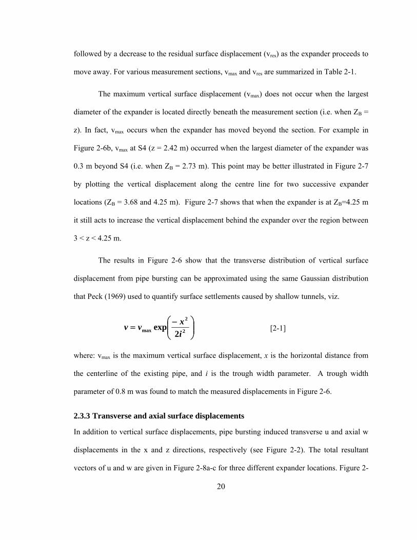
The results in Figure 2-6 show that the transverse distribution of vertical surface

displacement from pipe bursting can be approximated using the same Gaussian distribution

that Peck (1969) used to quantify surface settlements caused by shallow tunnels, viz.

⎟⎟⎠

⎞⎜⎜⎝

⎛ −= 2

2

max 2exp

ixvv [2-1]

where: vmax is the maximum vertical surface displacement, x is the horizontal distance from

the centerline of the existing pipe, and i is the trough width parameter. A trough width

parameter of 0.8 m was found to match the measured displacements in Figure 2-6.

2.3.3 Transverse and axial surface displacements

In addition to vertical surface displacements, pipe bursting induced transverse u and axial w

displacements in the x and z directions, respectively (see Figure 2-2). The total resultant

vectors of u and w are given in Figure 2-8a-c for three different expander locations. Figure 2-

21

8a shows that in advance of the expander the surface moves away from the centerline in the

transverse direction and forward in the axial direction. Once the expander has passed any

given point, while the soil at the surface continues to move away from the centerline in the

transverse direction, it moves backwards in the axial direction. Figure 2-8c shows net

backward (i.e. negative w) axial displacements. From the incremental resultant vectors in

Figure 2-8d-e, it can be seen that the incremental u-components are greater in the vicinity of

the expander, while behind the expander, incremental resultant vectors are dominated by the

w-component.

To better illustrate the three-dimensional nature of the surface displacements, the

displacement trajectory in the (z, y) plane of a target located at x = 0 m and z = 4.88 m is

given in Figure 2-9. Upward vertical (v) and forward axial (w) displacements are taken as

positive. As the expander approaches, the target displaces forward and upward. The

maximum forward position is reached when the expander is roughly beneath the target (ZB =

4.92 m). When the expander advances further into the soil (from ZB = 4.92 m to ZB = 5.95

m), the target moves backward and slightly upward. Here, the incremental axial displacement

is -1.1 mm. The net displacement of the target (from ZB = 0.00 to 7.47 m) was upward by 5.5

mm and backward by -0.6 mm.

The displacement trajectories in the (x, z) plane of two points located at z = 3.96 m

and each 1 m from the centerline are given in Figure 2-10. Forward axial (w) displacements

are taken as positive and transverse (u) displacements to the right of the centerline are taken

as positive. As shown in Figure 2-9, axial displacements are positive until the expander is in

the vicinity of the section, from which time backward movements occur. Transverse

displacements increase as the expander approaches and continue to do so as the expander

moves beyond the section. Here, the maximum transverse displacement is 1.3 mm.

22

A zone of tension is created as the ground surface is displaced away from the

centerline of the existing pipe. Acting within the zone of tension are tensile strains which

could lead to the formation of tension cracks. Figure 2-11a gives transverse displacements (u)

for z = 6.43 m when ZB = 6.93 m. There is a discontinuity in the transverse displacements of

0.5 mm at -0.62 m < x < -0.42 m (Figure 2-11a). There is an intermediate zone at -0.42 m < x

< 0.20 m which displaces horizontally an average of -0.4 mm. A more significant

discontinuity of 1.6 mm occurs at 0.20 m < x < 0.28 m. At this location the direction of u

changes (u > 0 mm when x > 0.25 m and u < 0 mm when x < 0.25 m) which indicates surface

spreading. It would be expected that this would produce the highest tensile strains making it

the most susceptible to tension cracks. In fact, upon completion of the pipe bursting

experiment, two distinct tension cracks were observed on the surface. The location of the

surface tension cracks are shown in Figure 2-8b. The first was 0.48 m in length extending

from z = 2.44 m to z = 2.88 m located between -0.30 m < x < -0.18 m. The second crack was

3.65 m in length extending from z = 3.53 m to z = 7.01 m located between -0.11 m < x < 0.38

m.

Using small-displacement theory, the horizontal strain can be approximated by:

xu

xu

xx ΔΔ

=∂∂

=ε [2-2]

where: Δu is the incremental transverse surface displacement and Δx is the incremental

transverse distance. The computed horizontal strains for z = 6.43 m when ZB = 6.93 m are

given in Figure 2-11b with tensile strains taken as positive (calculation details are provided in

Appendix C). The tensile zone is located between -0.87 m < x < 0.82 m. Two peak tensile

strains occur in the tensile zone. The first strain peak of 0.27% occurs at x = -0.61 m. The

second strain peak reaches 13.42% at x = 0.27 m. Substantially larger strains occur at x =

23

0.27 m, which is consistent with the tension crack observed at x = 0.22 m shown in Figure 2-

8b.

It is uncertain whether the observed cracking would have developed if either a

bituminous or concrete pavement was present on the ground surface. In fact, the surface

displacements presented in this chapter are conservative for the pipe bursting geometry tested

since if an overlying pavement or structure was present, it would restrain (i.e. decrease)

ground surface displacements. Further investigation is required to determine the magnitude

and impact of surface displacements with an overlying pavement layer, and the likelihood of

damage to the pavement.

2.4 Conclusions

Experimental results from a laboratory investigation of static pipe bursting in a well-graded

sand and gravel soil were presented. The experiment was conducted in an 8-m-long, 8-m-

wide, and 3-m-deep test pit with an unreinforced concrete pipe (buried 1.385 m below the

ground surface) being replaced by a high-density polyethylene pipe. The pulling force and

three-dimensional surface displacements were quantified leading to the following

conclusions specific to the conditions tested:

(i) The average force required to break the existing pipe, expand the soil cavity and

move the expander forward, and overcome friction on the replacement pipe was

149 kN, and the maximum force was 209 kN. The observed variations in pulling

force were largely attributed to crack initiation and propagation in the concrete

pipe. The largest component of the measured pull force (100–130 kN) was that to

expand the soil cavity and move the expander forward.

24

(ii) The maximum vertical displacement at any point occurred once the expander had

progressed beyond that point. This was attributed to the incremental change in

vertical displacement as the expander is pulled through the existing pipe.

(iii) Vertical surface displacements increased until z = 4.92 m when a maximum

vertical surface displacement of 6 mm was reached. Beyond this, displacements

were influenced by the rigid end boundary. The transverse distribution of vertical

displacements for this experimental geometry can be approximated using a

Gaussian distribution with a trough width parameter of 0.8 m.

(iv) As the expander approached a given section, a point on the surface at that section

moved vertically upwards, transversely outwards, and axially forwards. The

permanent surface displacement (i.e. once the expander had passed) was

vertically upwards, transversely outwards, and axially backwards from its original

position.

(v) The sand and gravel surface (tested without pavement) was cracked from

transverse tensile strains close to points directly above the pipe centerline.

2.5 References

Lapos, B.M. 2004. Laboratory study of static pipe bursting three-dimensional ground

displacements and pull force during installation, and subsequent response of HDPE

replacement pipes under surcharge loading. M.Sc. Thesis, Dept. of Civil Engineering,

Queen’s University, Kingston, Ont.

Peck, R. B. 1969. Deep excavations and tunnelling in soft ground. Proc. 7th Int.l Conf.

Soil Mechanics and Foundation Engineering, Mexico City, vol.1, 225-290

Rogers, C.D.F., and Chapman, D.N. 1995. An experimental study of pipebursting in sand.

Proc., Inst. Civ. Eng., London, 113(1), 38-50.

25

Scott, J.D., Bauer, G.E., and Shields, D.H. 1977. Triaxial testing on granular A aggregate.

Ontario joint transportation and communications research program. Project O-1.

Simicevic, J., and Sterling, R.L. 2001. Guidelines for pipe bursting. TTC technical report

#2001.02, U.S. Army Corps of Engineers.

White, D.J., Take, W.A. and Bolton, M.D. 2003. Soil deformation measurement using

particle image velocimetry (PIV) and photogrammetry. Geotechnique 53 (7):619-631.

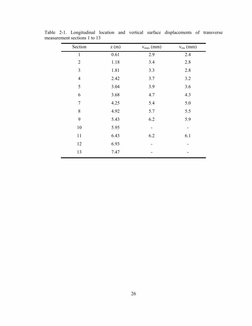
26

Table 2-1. Longitudinal location and vertical surface displacements of transverse measurement sections 1 to 13

Section z (m) vmax (mm) vres (mm)

1 0.61 2.9 2.4 2 1.18 3.4 2.8

3 1.81 3.3 2.8

4 2.42 3.7 3.2

5 3.04 3.9 3.6

6 3.68 4.7 4.3

7 4.25 5.4 5.0

8 4.92 5.7 5.5

9 5.43 6.2 5.9

10 5.95 - -

11 6.43 6.2 6.1

12 6.93 - -

13 7.47 - -

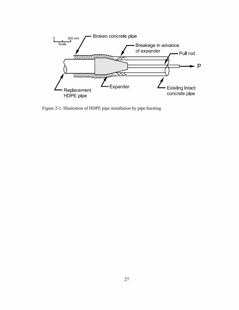
27

Figure 2-1. Illustration of HDPE pipe installation by pipe bursting

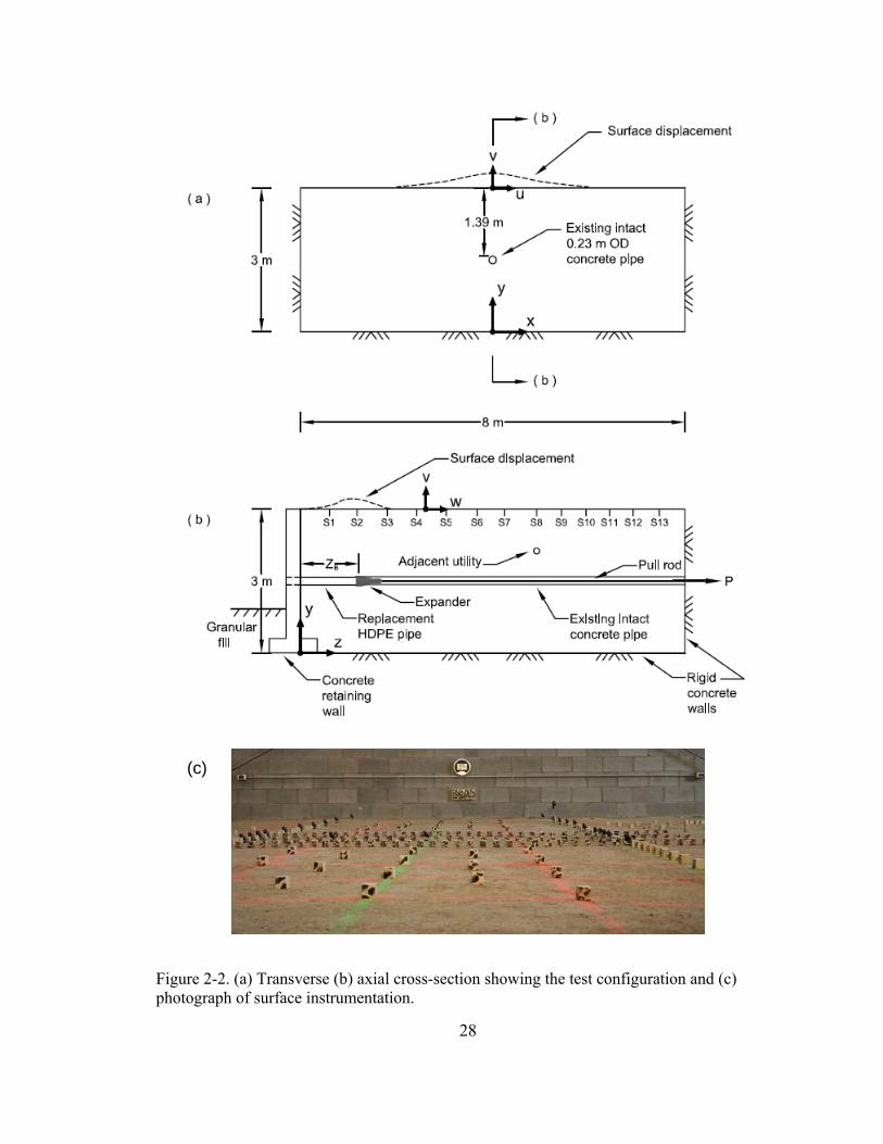
28

(c)

Figure 2-2. (a) Transverse (b) axial cross-section showing the test configuration and (c) photograph of surface instrumentation.

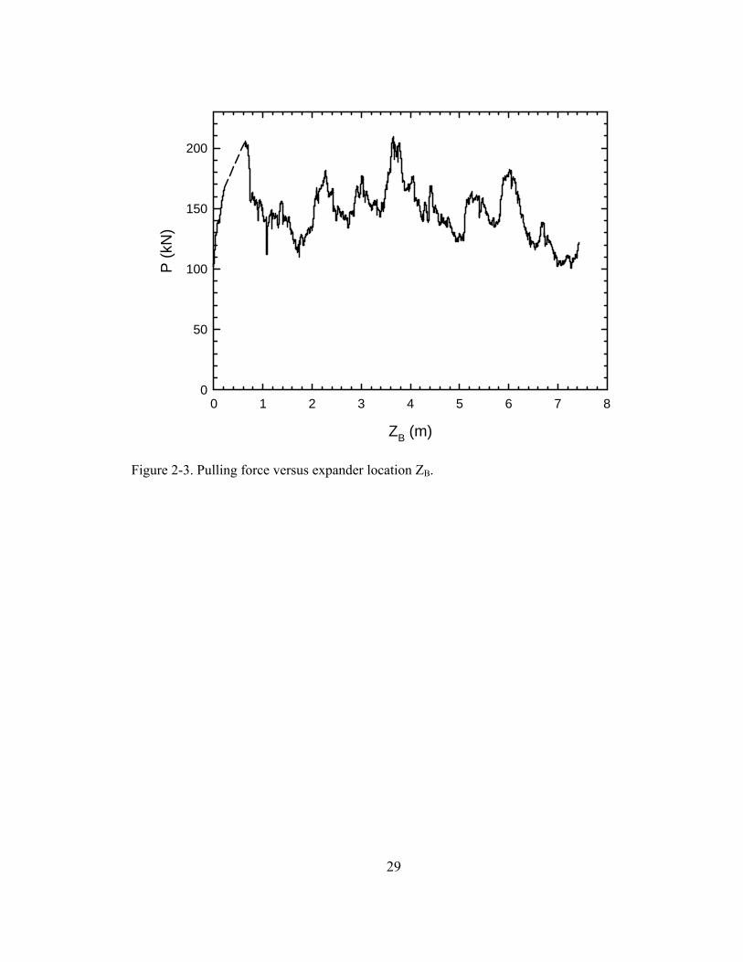
29

ZB (m)

0 1 2 3 4 5 6 7 8

P (k

N)

0

50

100

150

200

Figure 2-3. Pulling force versus expander location ZB.

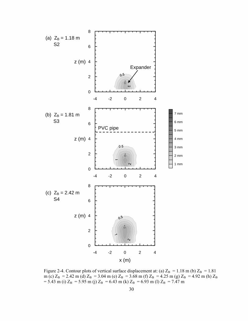
30

-4 -2 0 2 40

2

4

6

8

z (m)

-4 -2 0 2 40

2

4

6

8

z (m)

1 mm

2 mm

3 mm

4 mm

5 mm

6 mm

7 mm

-4 -2 0 2 4

x (m)

0

2

4

6

8

z (m)

Figure 2-4. Contour plots of vertical surface displacement at: (a) ZB = 1.18 m (b) ZB = 1.81 m (c) ZB = 2.42 m (d) ZB = 3.04 m (e) ZB = 3.68 m (f) ZB = 4.25 m (g) ZB = 4.92 m (h) ZB = 5.43 m (i) ZB = 5.95 m (j) ZB = 6.43 m (k) ZB = 6.93 m (l) ZB = 7.47 m

(a) ZB = 1.18 m S2

(b) ZB = 1.81 m S3

(c) ZB = 2.42 m S4

Expander

PVC pipe

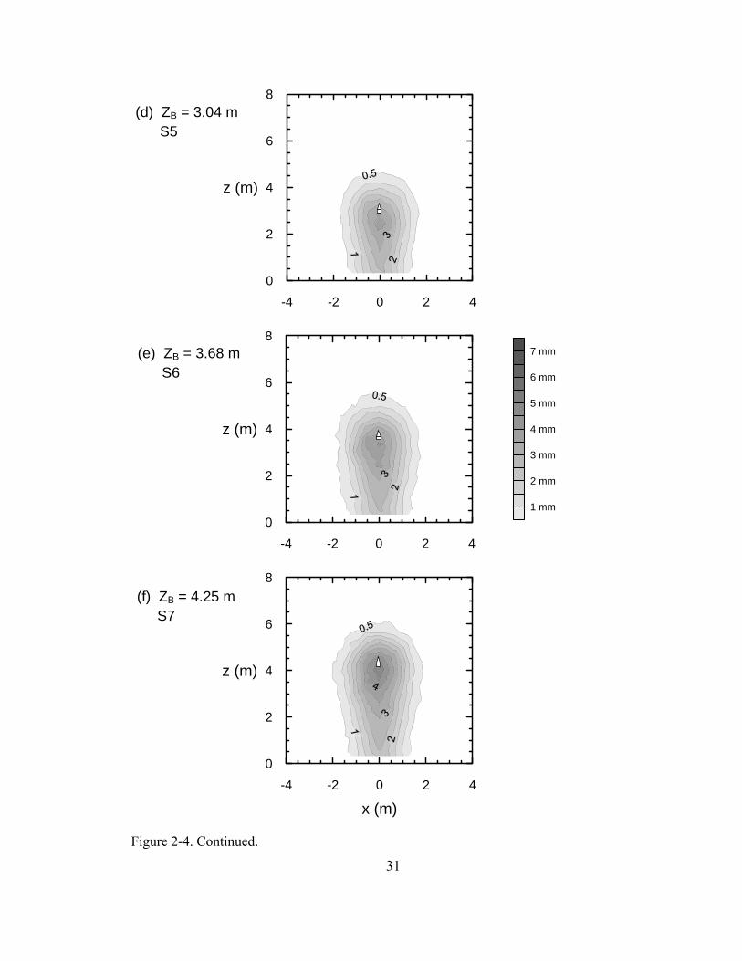
31

-4 -2 0 2 40

2

4

6

8

z (m)

-4 -2 0 2 40

2

4

6

8

z (m)

1 mm

2 mm

3 mm

4 mm

5 mm

6 mm

7 mm

-4 -2 0 2 4

x (m)

0

2

4

6

8

z (m)

Figure 2-4. Continued.

(d) ZB = 3.04 m S5

(e) ZB = 3.68 m S6

(f) ZB = 4.25 m S7

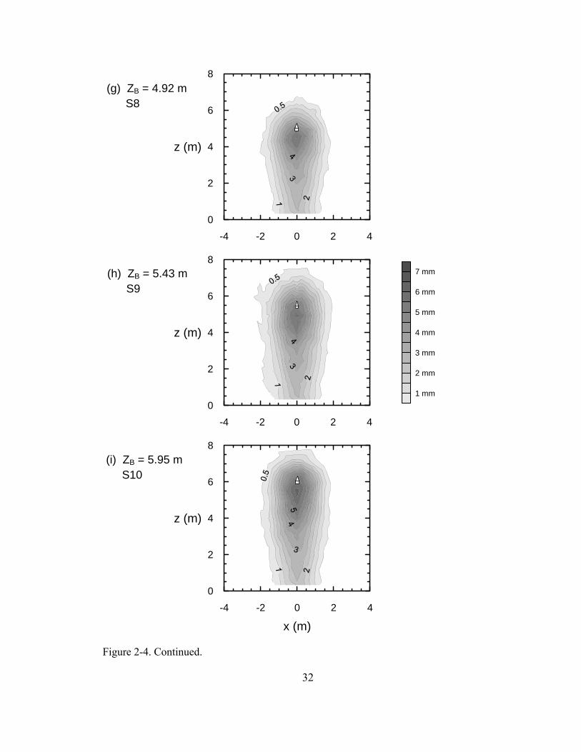
32

-4 -2 0 2 40

2

4

6

8

z (m)

-4 -2 0 2 40

2

4

6

8

z (m)

1 mm

2 mm

3 mm

4 mm

5 mm

6 mm

7 mm

-4 -2 0 2 4

x (m)

0

2

4

6

8

z (m)

Figure 2-4. Continued.

(g) ZB = 4.92 m S8

(h) ZB = 5.43 m S9

(i) ZB = 5.95 m S10

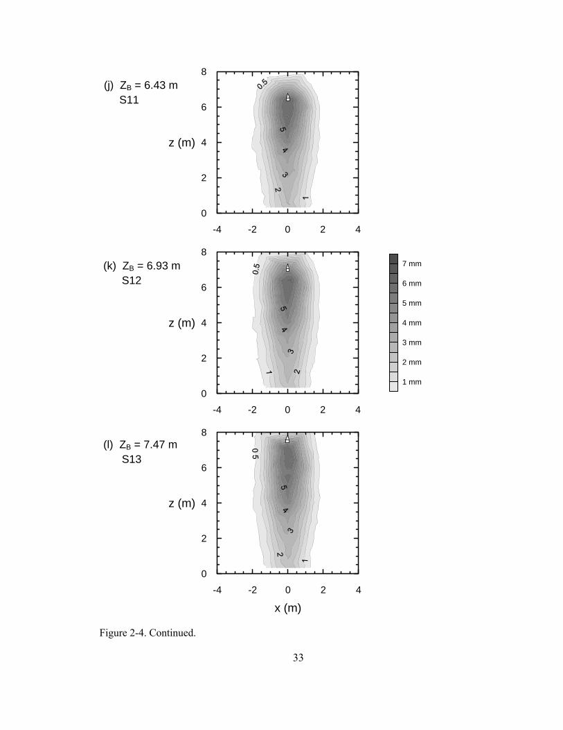
33

-4 -2 0 2 40

2

4

6

8

z (m)

-4 -2 0 2 40

2

4

6

8

z (m)

1 mm

2 mm

3 mm

4 mm

5 mm

6 mm

7 mm

-4 -2 0 2 4

x (m)

0

2

4

6

8

z (m)

Figure 2-4. Continued.

(j) ZB = 6.43 m S11

(k) ZB = 6.93 m S12

(l) ZB = 7.47 m S13

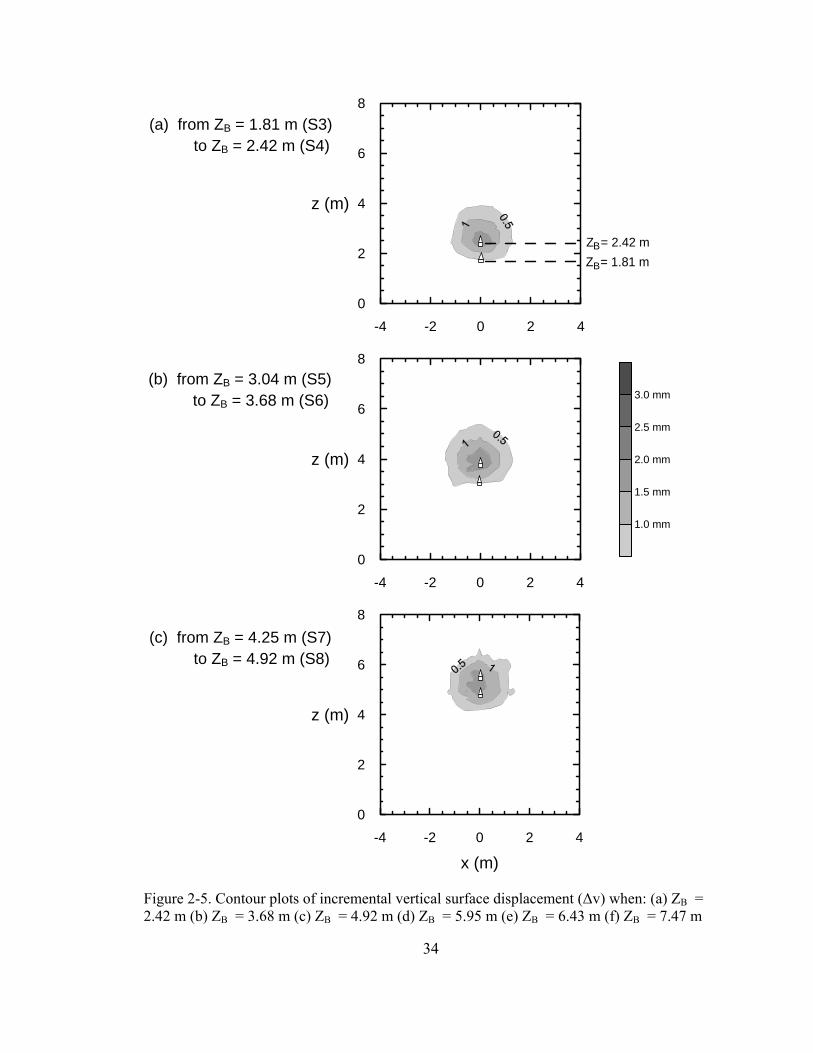
34

-4 -2 0 2 40

2

4

6

8

z (m)

Z = 2.42 mZ = 1.81 mB

B

-4 -2 0 2 40

2

4

6

8

z (m)

1.0 mm

1.5 mm

2.0 mm

2.5 mm

3.0 mm

-4 -2 0 2 4

x (m)

0

2

4

6

8

z (m)

Figure 2-5. Contour plots of incremental vertical surface displacement (Δv) when: (a) ZB = 2.42 m (b) ZB = 3.68 m (c) ZB = 4.92 m (d) ZB = 5.95 m (e) ZB = 6.43 m (f) ZB = 7.47 m

(b) from ZB = 3.04 m (S5) to ZB = 3.68 m (S6)

(a) from ZB = 1.81 m (S3) to ZB = 2.42 m (S4)

(c) from ZB = 4.25 m (S7) to ZB = 4.92 m (S8)

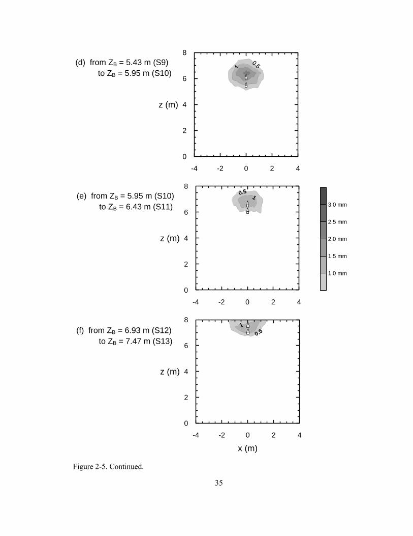
35

-4 -2 0 2 40

2

4

6

8

z (m)

-4 -2 0 2 40

2

4

6

8

z (m)

1.0 mm

1.5 mm

2.0 mm

2.5 mm

3.0 mm

0.51

-4 -2 0 2 4

x (m)

0

2

4

6

8

z (m)

0.51

Figure 2-5. Continued.

(d) from ZB = 5.43 m (S9) to ZB = 5.95 m (S10)

(e) from ZB = 5.95 m (S10) to ZB = 6.43 m (S11)

(f) from ZB = 6.93 m (S12) to ZB = 7.47 m (S13)

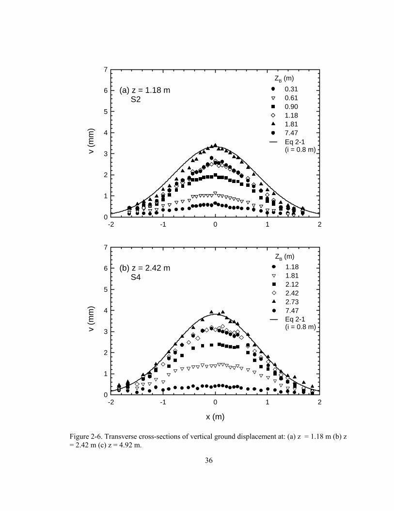
36

-2 -1 0 1 2

v (m

m)

0

1

2

3

4

5

6

7

0.310.610.901.181.817.47

ZB (m)

(a) z = 1.18 m S2

Eq 2-1(i = 0.8 m)

x (m)

-2 -1 0 1 2

v (m

m)

0

1

2

3

4

5

6

7

1.181.812.122.422.737.47

ZB (m)

(b) z = 2.42 m S4

Eq 2-1(i = 0.8 m)

Figure 2-6. Transverse cross-sections of vertical ground displacement at: (a) z = 1.18 m (b) z = 2.42 m (c) z = 4.92 m.

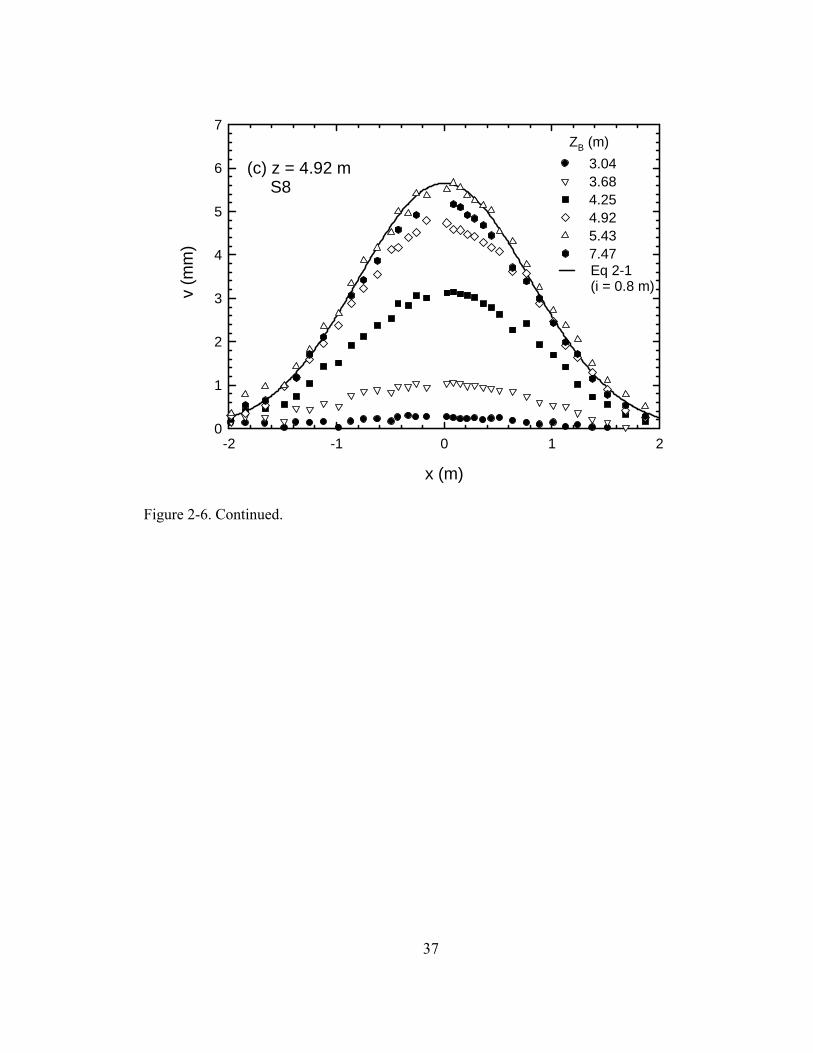
37

x (m)

-2 -1 0 1 2

v (m

m)

0

1

2

3

4

5

6

7

3.043.684.254.925.437.47

ZB (m)

(c) z = 4.92 m S8

Eq 2-1(i = 0.8 m)

Figure 2-6. Continued.

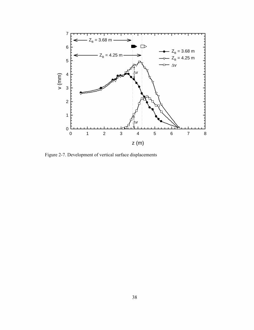
38

z (m)

0 1 2 3 4 5 6 7 8

v (m

m)

0

1

2

3

4

5

6

7

ZB = 3.68 mZB = 4.25 mΔv

Δv

Δv

ZB = 3.68 m

ZB = 4.25 m

Figure 2-7. Development of vertical surface displacements

39

-4 -2 0 2 40

2

4

6

8

z (m

)

-4 -2 0 2 40

2

4

6

8

z (m

)

-4 -2 0 2 40

2

4

6

8

z (m

)

1.0 mm

1.0 mm

-4 -2 0 2 4

x (m)

0

2

4

6

8

z (m

)

1.0 mm

Z = 5.95 m B

Z = 3.04 m B

Z = 4.92 m B

1.0 mm

-4 -2 0 2 4

x (m)

0

2

4

6

8z

(m)

1.0 mm

= Expander

= Expander

= Expander

from Z = 3.04 m ( )Bto Z = 4.92 m ( )B

from Z = 4.92 m ( )Bto Z = 5.95 m ( )B

(a)

(b)

(c)

(d)

(e)Observed tension crack

Δw

Δu

Δw

Δu

w

u

w

u

w

u

Figure 2-8. Total resultant vectors of u and w displacements when: (a) ZB = 3.04 m (b) ZB = 4.92 m (c) ZB = 5.95 m, and incremental resultant vectors when: (d) ZB = 4.92 m (e) ZB = 5.95 m.

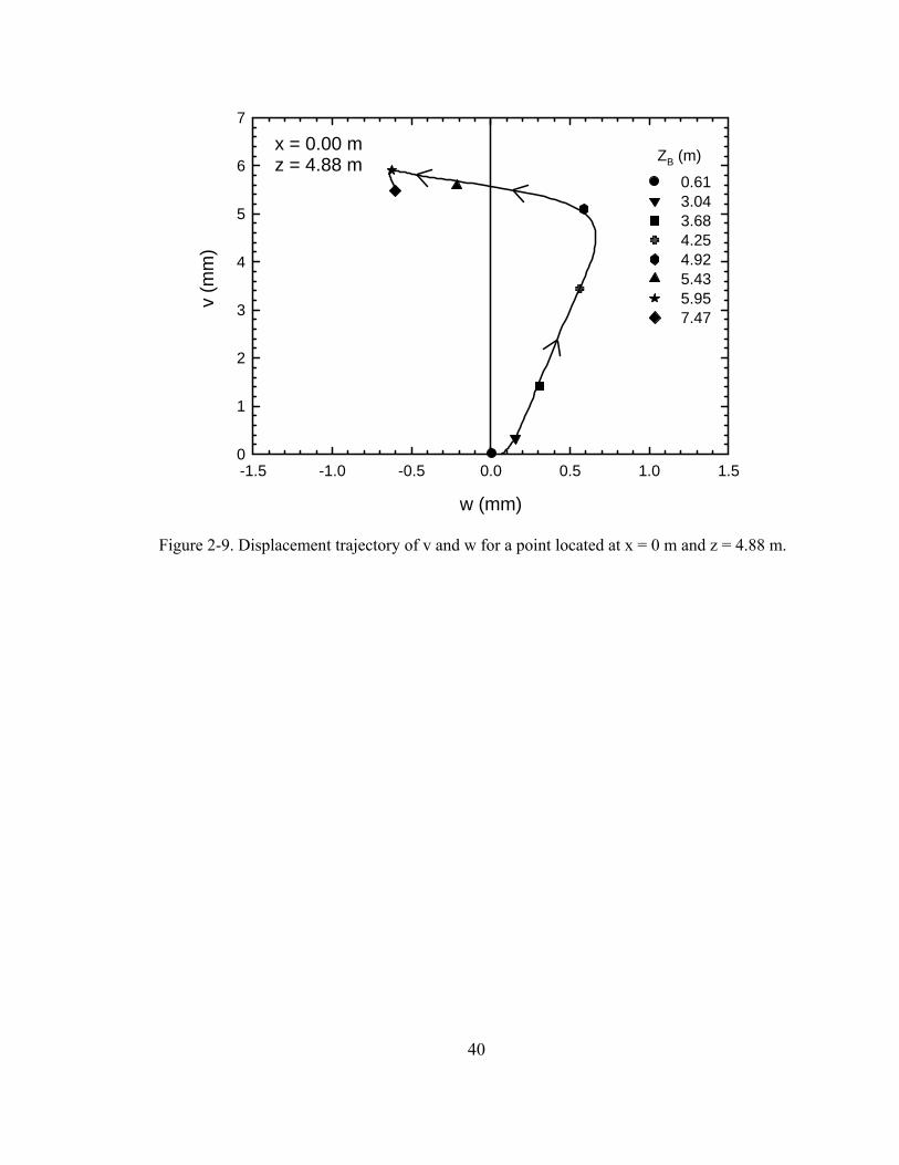
40

w (mm)

-1.5 -1.0 -0.5 0.0 0.5 1.0 1.5

v (m

m)

0

1

2

3

4

5

6

7

0.613.043.684.254.925.435.957.47

ZB (m)x = 0.00 mz = 4.88 m

Figure 2-9. Displacement trajectory of v and w for a point located at x = 0 m and z = 4.88 m.

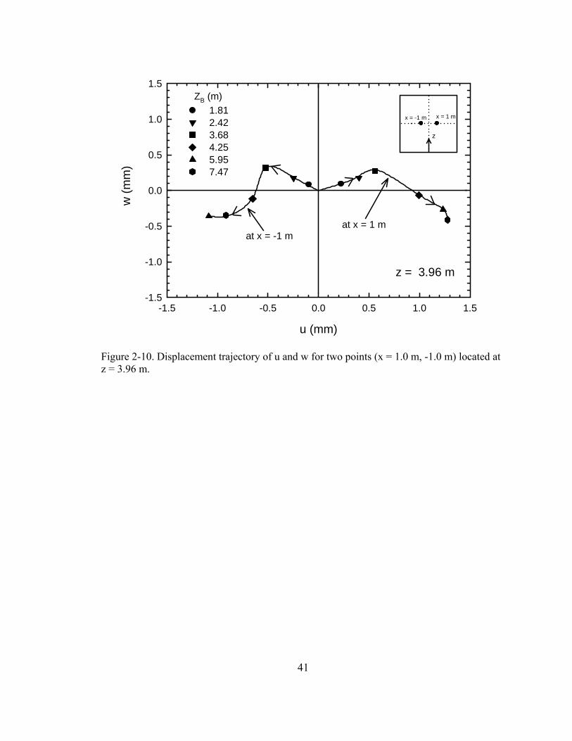
41

1.812.423.684.255.957.47

u (mm)

-1.5 -1.0 -0.5 0.0 0.5 1.0 1.5

w (m

m)

-1.5

-1.0

-0.5

0.0

0.5

1.0

1.5ZB (m)

z = 3.96 m

x = 1 mx = -1 m

z

at x = -1 m at x = 1 m

Figure 2-10. Displacement trajectory of u and w for two points (x = 1.0 m, -1.0 m) located at z = 3.96 m.

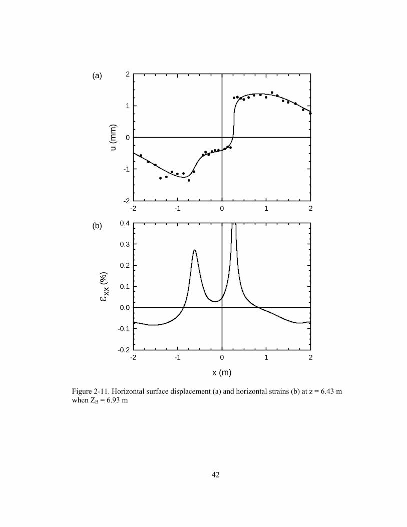
42

-2 -1 0 1 2

u (m

m)

-2

-1

0

1

2

x (m)

-2 -1 0 1 2

ε xx

(%)

-0.2

-0.1

0.0

0.1

0.2

0.3

0.4

Figure 2-11. Horizontal surface displacement (a) and horizontal strains (b) at z = 6.43 m when ZB = 6.93 m

(a)

(b)

43

Chapter 3

Response of a PVC water pipe when transverse to the replacement

of an underlying pipe by pipe bursting

3.1 Introduction

An existing deteriorated or hydraulically undersized pipe (made of brittle material) can be

replaced with a new pipe by static pipe bursting (e.g., see Simicevic and Sterling, 2001). As

shown in Figure 3-1, this process involves breaking (i.e. bursting) the existing pipe by using

an expander that is pulled by a series of rods. The broken pipe fragments are forced out into

the surrounding soil. In addition, the expander also enlarges the soil cavity if the diameter of

the expander is greater than that of the existing pipe. The replacement pipe is attached to the

rear of the expander and is pulled-into-place along the same trajectory as the existing pipe.

Of specific interest in this work is the affect of the ground movements, caused by cavity

expansion, on an adjacent utility running above and transverse to the existing pipe being

replaced.

Physical pipe bursting experiments have been conducted to quantify the three-

dimensional nature of surface and sub-surface ground displacements (Rogers and Chapman,

1995; Lapos et al., 2004) and procedures have been developed for estimating the magnitude

of these displacements as a result of cavity expansion (Nkemitag and Moore, 2006). There

have been limited experimental studies that investigate the response of an adjacent polyvinyl

chloride pipe to ground displacements caused by pipe bursting. Atalah (1998) monitored

pressure in transverse polyvinyl chloride pipes in the vicinity of pipe bursting operations.

During one particular test in sand, the polyvinyl chloride pipe crossing 300 mm above the

clay pipe being upsized by 50% lost internal pressure, suggesting the pipe was damaged. For

44

cases when internal pressure was maintained, the short-term capacity of the pipe may not

have been exceeded; however, of particular interest are the strains that developed in these

pipes to determine if long-term performance limits were exceeded. Currently, proximity

charts are available to identify whether or not the integrity of grey cast iron pipes would be in

jeopardy if pipe bursting operations were performed in its vicinity (Transco, 1997); however,

these charts have been developed on the basis of very limited field studies (Chapman et al.,

2007).

Therefore, the objective of this chapter is to quantify the response of a polyvinyl

chloride pipe, representing a utility in the vicinity of a pipe bursting operation. A large-scale

pipe bursting experiment was performed, with the polyvinyl chloride pipe crossing transverse

and 0.45 m above the pipe being replaced. The measured strain and corresponding deflection

of the polyvinyl chloride pipe are presented. In addition, an equation for estimating the

magnitude of maximum longitudinal strain in the adjacent utility is evaluated.

3.2 Experimental details

3.2.1 Test Pit

A schematic of the static pipe bursting experiment is provided in Figure 3-1. It was

performed in an 8-m-long, 8-m-wide, and 3-m-deep test pit with boundary conditions

consisting of three rigid concrete walls at: (a) z = 8 m, x= -4 m to 4 m; (b) x = -4 m, z = 0 m

to 8 m; and (c) x = 4 m, z = 0 m to 8 m. The fourth wall at z = 0 m, x= -4 m to 4 m is a

removable concrete retaining partition (i.e. the test pit is actually 16 m long) anchored to the

concrete floor and buttressed with granular fill to reduce horizontal displacement at the top of

the wall. In Chapter 2, it was shown that, given the size of the test pit, the imposed restraint

from boundary friction did not affect the ground displacements in the vicinity of the

45

polyvinyl chloride pipe. The expander and replacement pipe entered the test pit through a

porthole located at x = 0 m and z = 0 m. The 8-m-long replacement pipe was strung out in the

adjacent partially empty pit, and it was pulled towards another porthole at x = 0 m and z = 8

m.

3.2.2 Materials

A well-graded sand and gravel, having a coefficient of uniformity (Cu) of 20 and a coefficient

of curvature (Cc) of 0.5, was used to fill the test pit. The material had a maximum and

minimum dry density of 2.46 g/cm3 and 1.87 g/cm3, respectively. It was placed in 300-mm-

thick lifts and compacted, using a vibrating plate tamper (Wacker 1550 with an operating

mass of 88 kg and a maximum centrifugal force of 15 kN), to an average as-placed dry

density of 2.13 ± 0.01 g/cm3 at an average water content of 4.6 ± 0.9 % (where ± is one

standard deviation).

The unreinforced concrete pipe being burst, located along x = 0 m, had an outside

diameter (OD) of 229 mm and an average wall thickness of 38 mm. It was replaced with a

high-density polyethylene (HDPE) pipe with an OD of 168 mm and an average wall

thickness of 11 mm. Buried above and transverse to the concrete pipe along z = 4.92 m was

an polyvinyl chloride (PVC) pipe with an OD of 122 mm and an average wall thickness of 7

mm. There was 815 mm of cover above the PVC pipe (crown to the surface) and the vertical

distance between the invert of the PVC pipe and the crown of the concrete pipe was 450 mm.

The configurations of the PVC pipe and the concrete pipe are illustrated in Figures 3-1 and 3-

2.

46

3.2.3 Instrumentation

During the pipe bursting process, surface displacements directly above the PVC pipe and

strains in the PVC pipe were monitored. Surface displacements (v and w in the y and z

directions, respectively, as defined in Figure 3-1) were measured using targets tracked with

digital cameras and surveying prisms electronically tracked with a total station. Images

obtained from the cameras were analyzed using the image-based deformation software,

geoPIV (White et al., 2003). The accuracy of the displacements obtained with the cameras

and the total station are ± 0.1 mm and ± 0.3 mm respectively.

The outside surface of the PVC pipe was instrumented at 13 separate sections along

the length of the pipe with 52 uniaxial and rosette strain gages fixed at the crown, invert, and

two springlines. The uniaxial (Showa N11-FA-5-120-11) and rosette (Showa N32-FA-5-120-

11) foil strain gages had a gage length of 5 mm and were estimated to be accurate to within

±10 microstrain (με). These gages were used to measure strains in the longitudinal (x) and

circumferential (θ) direction as defined in Figure 3-3. Tensile longitudinal (εx) and

circumferential (εθ) strains are taken as positive. The strain measured was multiplied by a

modification factor of 1.2 to account for local gage stiffening. This factor was obtained in a

separate experiment by dividing strain calculated from independent deflection measurements

by measurements with the strain gages during an unrestrained thermal expansion/contraction

test from 0oC to 30oC. The strain gage readings were zeroed after backfilling of the PVC pipe

was complete. Measurements of longitudinal strain in the PVC pipe were used to infer pipe

displacements v and w shown in Figure 3-2. To measure vertical movement of the PVC pipes

ends during the pipe bursting process, metal rods attached to the pipe crown at x = -3 and 3 m

were extended up to and beyond the ground surface, and a surveying prism was mounted at

the top as shown in Figure 3-1.

47

3.2.4 Method

This pipe bursting experiment was performed using an expander with a maximum diameter

of 202 mm (Figure 3-2). Steel pull rods connected the expander to a hydraulic actuator which

was used to pull the expander and replacement HDPE pipe through the concrete pipe at a

controlled displacement rate of 100 mm/min. The pulling process was paused for 15-20

minutes at various expander locations (denoted as ZB in Figure 3-1) to take measurements of

surface displacements and pipe strains. For ZB = 4.92 m, the expander was directly beneath

the PVC pipe located at z = 4.92 m.

3.3 Results

3.3.1 Longitudinal strains in the PVC pipe

The distribution of longitudinal strains εx measured along the crown and invert of the PVC

pipe for ZB = 4.25 and 4.92 m are given in Figure 3-4. In addition, the measured longitudinal

strains at the crown and invert for various expander locations are given in Table 3-1 and 3-2

respectively. Tensile strains are taken as positive. When ZB = 1.18 m, longitudinal strain

began to develop in the PVC pipe and continued to increase as the expander approached the

pipe at z = 4.92 m. When ZB > 4.25 m, bending developed in the PVC pipe near the

centreline of the existing concrete pipe being burst (indicated by tensile strains measured

along the crown and compressive strains along the invert). As expected, the strains measured

on the crown and invert are nearly equal but opposite and almost symmetric about x = 0.

When the expander was directly beneath the PVC pipe (ZB = 4.92 m), the maximum

longitudinal strain of 880 με was measured (corresponding to about 0.09% strain) at x = 0.

Subsequent strain measurements at the crown and invert remain almost constant when the

expander moved beyond the PVC pipe (i.e. from ZB = 4.92 m to ZB = 7.47 m).

The curvature κ of the PVC pipe can be calculated by:

48

Dεε

κ ic - = [3-1]

where: εc is the strain measured at the crown, εi is the strain measured at the invert, and D is

the outside diameter of the PVC pipe. The computed curvature of the PVC pipe when ZB =

4.25 m and 4.92 m is given in Figure 3-5. Here, it is further illustrated that the maximum

bending (or maximum curvature) occurs at a portion of the PVC pipe located directly above

the pipe being replaced (x = 0) and bending of the PVC pipe increases as the expander

approached (from ZB = 4.25 m to 4.92 m).

3.3.2 PVC pipe and surface displacements

Using conventional thin beam theory, the vertical displacement v of the PVC pipes centroid

can be related to its curvature κ by:

2

2

=dx

vdκ [3-2]

Using this expression and integrating curvature twice (with specific details provided in

Appendix D), the distribution of vertical displacements for the PVC pipe was calculated, for

different stages of the experiment as the expander approached and moved beyond the PVC

pipe as given in Figure 3-6a. Upward vertical displacements are taken as positive. The PVC

pipe begins to displace vertically when the expander was approximately 1.88 m away (i.e. the

expander at ZB = 3.04 m). As the expander approached, vertical displacement increased to a

maximum of 5.1 mm when ZB = 5.43 m followed by a decrease to the residual vertical

displacement as the expander proceeded to move away. The displacements measured near the

ends of the pipe at x = -3 and 3 m during the experiment were negligible.

A transverse cross-section showing the vertical displacement of the ground surface

measured above the PVC pipe at z = 4.92 m is shown in Figure 3-6b. The ground surface

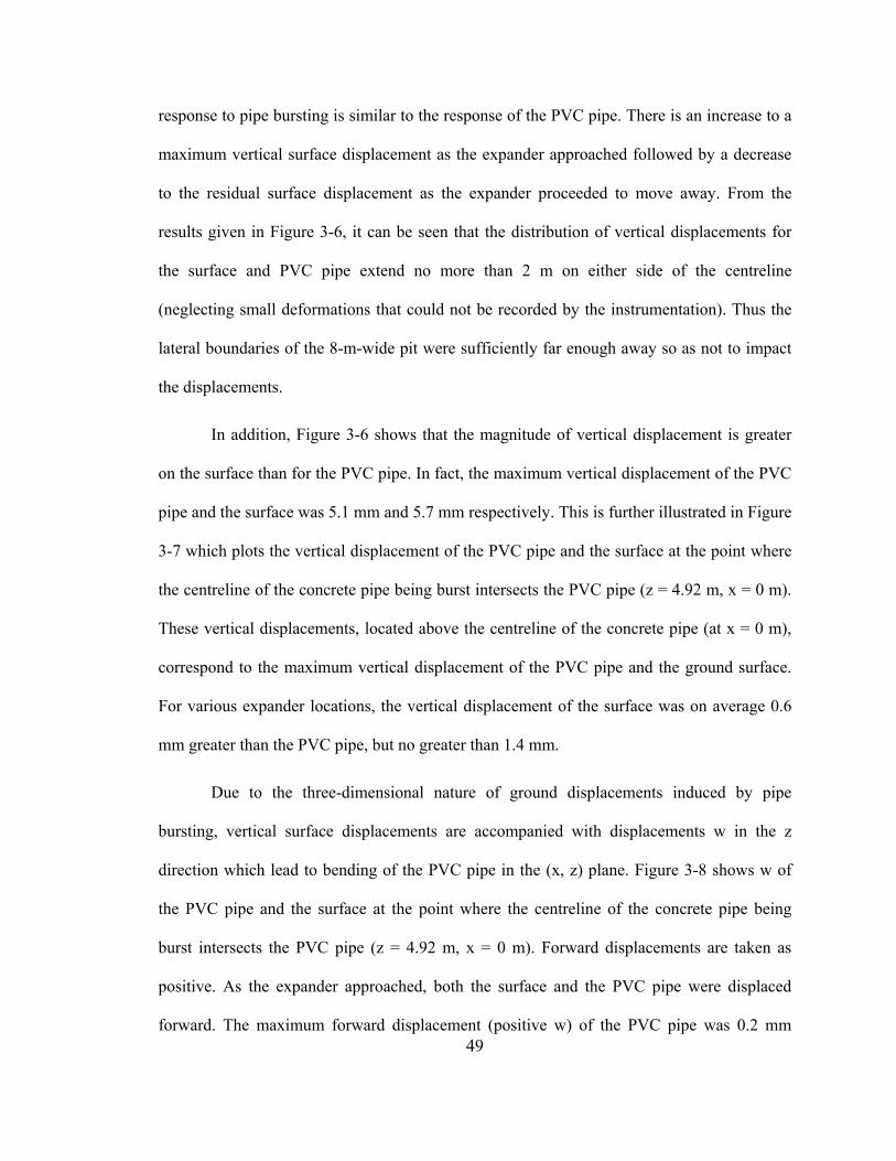
49

response to pipe bursting is similar to the response of the PVC pipe. There is an increase to a

maximum vertical surface displacement as the expander approached followed by a decrease

to the residual surface displacement as the expander proceeded to move away. From the

results given in Figure 3-6, it can be seen that the distribution of vertical displacements for

the surface and PVC pipe extend no more than 2 m on either side of the centreline

(neglecting small deformations that could not be recorded by the instrumentation). Thus the

lateral boundaries of the 8-m-wide pit were sufficiently far enough away so as not to impact

the displacements.

In addition, Figure 3-6 shows that the magnitude of vertical displacement is greater

on the surface than for the PVC pipe. In fact, the maximum vertical displacement of the PVC

pipe and the surface was 5.1 mm and 5.7 mm respectively. This is further illustrated in Figure

3-7 which plots the vertical displacement of the PVC pipe and the surface at the point where

the centreline of the concrete pipe being burst intersects the PVC pipe (z = 4.92 m, x = 0 m).

These vertical displacements, located above the centreline of the concrete pipe (at x = 0 m),

correspond to the maximum vertical displacement of the PVC pipe and the ground surface.

For various expander locations, the vertical displacement of the surface was on average 0.6

mm greater than the PVC pipe, but no greater than 1.4 mm.

Due to the three-dimensional nature of ground displacements induced by pipe

bursting, vertical surface displacements are accompanied with displacements w in the z

direction which lead to bending of the PVC pipe in the (x, z) plane. Figure 3-8 shows w of

the PVC pipe and the surface at the point where the centreline of the concrete pipe being

burst intersects the PVC pipe (z = 4.92 m, x = 0 m). Forward displacements are taken as

positive. As the expander approached, both the surface and the PVC pipe were displaced

forward. The maximum forward displacement (positive w) of the PVC pipe was 0.2 mm

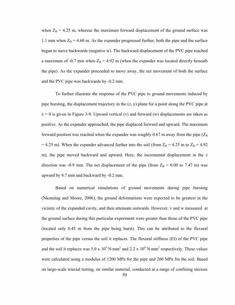
50

when ZB = 4.25 m, whereas the maximum forward displacement of the ground surface was

1.1 mm when ZB = 4.60 m. As the expander progressed further, both the pipe and the surface

began to move backwards (negative w). The backward displacement of the PVC pipe reached

a maximum of -0.7 mm when ZB = 4.92 m (when the expander was located directly beneath

the pipe). As the expander proceeded to move away, the net movement of both the surface

and the PVC pipe was backwards by -0.2 mm.

To further illustrate the response of the PVC pipe to ground movements induced by

pipe bursting, the displacement trajectory in the (z, y) plane for a point along the PVC pipe at

x = 0 is given in Figure 3-9. Upward vertical (v) and forward (w) displacements are taken as

positive. As the expander approached, the pipe displaced forward and upward. The maximum

forward position was reached when the expander was roughly 0.67 m away from the pipe (ZB

= 4.25 m). When the expander advanced further into the soil (from ZB = 4.25 m to ZB = 4.92

m), the pipe moved backward and upward. Here, the incremental displacement in the z

direction was -0.9 mm. The net displacement of the pipe (from ZB = 0.00 to 7.47 m) was

upward by 4.7 mm and backward by -0.2 mm.

Based on numerical simulations of ground movements during pipe bursting

(Nkemitag and Moore, 2006), the ground deformations were expected to be greatest in the

vicinity of the expanded cavity, and then attenuate outwards. However, v and w measured at

the ground surface during this particular experiment were greater than those of the PVC pipe

(located only 0.45 m from the pipe being burst). This can be attributed to the flexural

properties of the pipe versus the soil it replaces. The flexural stiffness (EI) of the PVC pipe

and the soil it replaces was 5.0 x 109 N·mm2 and 2.2 x 109 N·mm2 respectively. These values

were calculated using a modulus of 1200 MPa for the pipe and 200 MPa for the soil. Based

on large-scale triaxial testing, on similar material, conducted at a range of confining stresses

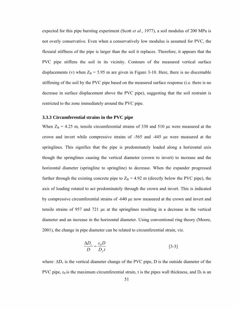
51

expected for this pipe bursting experiment (Scott et al., 1977), a soil modulus of 200 MPa is

not overly conservative. Even when a conservatively low modulus is assumed for PVC, the

flexural stiffness of the pipe is larger than the soil it replaces. Therefore, it appears that the

PVC pipe stiffens the soil in its vicinity. Contours of the measured vertical surface

displacements (v) when ZB = 5.95 m are given in Figure 3-10. Here, there is no discernable

stiffening of the soil by the PVC pipe based on the measured surface response (i.e. there is no

decrease in surface displacement above the PVC pipe), suggesting that the soil restraint is

restricted to the zone immediately around the PVC pipe.

3.3.3 Circumferential strains in the PVC pipe

When ZB = 4.25 m, tensile circumferential strains of 330 and 510 με were measured at the

crown and invert while compressive strains of -565 and -445 με were measured at the

springlines. This signifies that the pipe is predominately loaded along a horizontal axis

though the springlines causing the vertical diameter (crown to invert) to increase and the

horizontal diameter (springline to springline) to decrease. When the expander progressed

further through the existing concrete pipe to ZB = 4.92 m (directly below the PVC pipe), the

axis of loading rotated to act predominately through the crown and invert. This is indicated

by compressive circumferential strains of -640 με now measured at the crown and invert and

tensile strains of 957 and 721 με at the springlines resulting in a decrease in the vertical

diameter and an increase in the horizontal diameter. Using conventional ring theory (Moore,

2001), the change in pipe diameter can be related to circumferential strain, viz.

tD

DεDD

f

θv =Δ

[3-3]

where: ΔDv is the vertical diameter change of the PVC pipe, D is the outside diameter of the

PVC pipe, εθ is the maximum circumferential strain, t is the pipes wall thickness, and Df is an

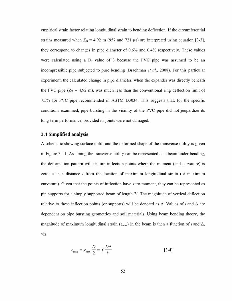
52

empirical strain factor relating longitudinal strain to bending deflection. If the circumferential

strains measured when ZB = 4.92 m (957 and 721 με) are interpreted using equation [3-3],

they correspond to changes in pipe diameter of 0.6% and 0.4% respectively. These values

were calculated using a Df value of 3 because the PVC pipe was assumed to be an

incompressible pipe subjected to pure bending (Brachman et al., 2008). For this particular

experiment, the calculated change in pipe diameter, when the expander was directly beneath

the PVC pipe (ZB = 4.92 m), was much less than the conventional ring deflection limit of

7.5% for PVC pipe recommended in ASTM D3034. This suggests that, for the specific

conditions examined, pipe bursting in the vicinity of the PVC pipe did not jeopardize its

long-term performance, provided its joints were not damaged.

3.4 Simplified analysis

A schematic showing surface uplift and the deformed shape of the transverse utility is given

in Figure 3-11. Assuming the transverse utility can be represented as a beam under bending,

the deformation pattern will feature inflection points where the moment (and curvature) is

zero, each a distance i from the location of maximum longitudinal strain (or maximum

curvature). Given that the points of inflection have zero moment, they can be represented as

pin supports for a simply supported beam of length 2i. The magnitude of vertical deflection

relative to these inflection points (or supports) will be denoted as Δ. Values of i and Δ are

dependent on pipe bursting geometries and soil materials. Using beam bending theory, the

magnitude of maximum longitudinal strain (εmax) in the beam is then a function of i and Δ,

viz.

2maxmax

Δ=

2=

iD

fD

κε [3-4]

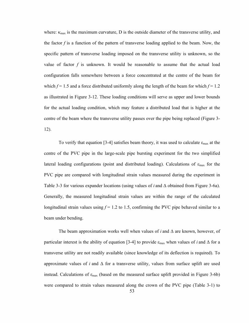
53

where: κmax is the maximum curvature, D is the outside diameter of the transverse utility, and

the factor f is a function of the pattern of transverse loading applied to the beam. Now, the

specific pattern of transverse loading imposed on the transverse utility is unknown, so the

value of factor f is unknown. It would be reasonable to assume that the actual load

configuration falls somewhere between a force concentrated at the centre of the beam for

which f = 1.5 and a force distributed uniformly along the length of the beam for which f = 1.2

as illustrated in Figure 3-12. These loading conditions will serve as upper and lower bounds

for the actual loading condition, which may feature a distributed load that is higher at the

centre of the beam where the transverse utility passes over the pipe being replaced (Figure 3-

12).

To verify that equation [3-4] satisfies beam theory, it was used to calculate εmax at the

centre of the PVC pipe in the large-scale pipe bursting experiment for the two simplified

lateral loading configurations (point and distributed loading). Calculations of εmax for the

PVC pipe are compared with longitudinal strain values measured during the experiment in

Table 3-3 for various expander locations (using values of i and Δ obtained from Figure 3-6a).

Generally, the measured longitudinal strain values are within the range of the calculated

longitudinal strain values using f = 1.2 to 1.5, confirming the PVC pipe behaved similar to a

beam under bending.

The beam approximation works well when values of i and Δ are known, however, of

particular interest is the ability of equation [3-4] to provide εmax when values of i and Δ for a

transverse utility are not readily available (since knowledge of its deflection is required). To

approximate values of i and Δ for a transverse utility, values from surface uplift are used

instead. Calculations of εmax (based on the measured surface uplift provided in Figure 3-6b)

were compared to strain values measured along the crown of the PVC pipe (Table 3-1) to

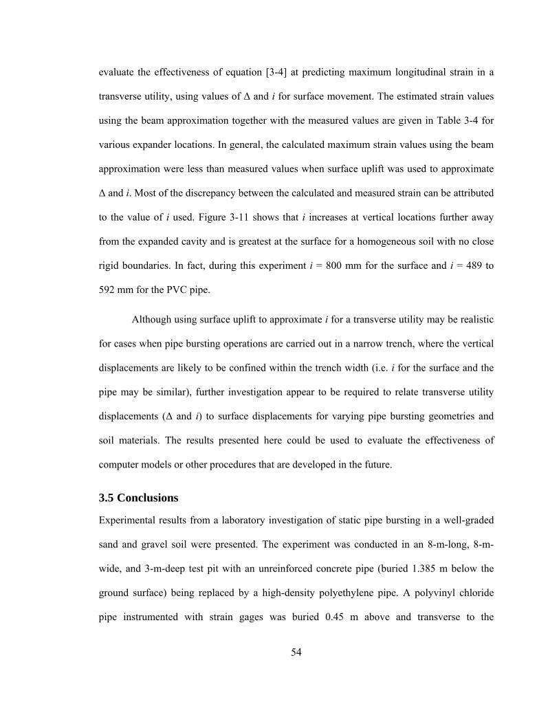
54

evaluate the effectiveness of equation [3-4] at predicting maximum longitudinal strain in a

transverse utility, using values of Δ and i for surface movement. The estimated strain values

using the beam approximation together with the measured values are given in Table 3-4 for

various expander locations. In general, the calculated maximum strain values using the beam

approximation were less than measured values when surface uplift was used to approximate

Δ and i. Most of the discrepancy between the calculated and measured strain can be attributed

to the value of i used. Figure 3-11 shows that i increases at vertical locations further away

from the expanded cavity and is greatest at the surface for a homogeneous soil with no close

rigid boundaries. In fact, during this experiment i = 800 mm for the surface and i = 489 to

592 mm for the PVC pipe.

Although using surface uplift to approximate i for a transverse utility may be realistic

for cases when pipe bursting operations are carried out in a narrow trench, where the vertical

displacements are likely to be confined within the trench width (i.e. i for the surface and the

pipe may be similar), further investigation appear to be required to relate transverse utility

displacements (Δ and i) to surface displacements for varying pipe bursting geometries and

soil materials. The results presented here could be used to evaluate the effectiveness of

computer models or other procedures that are developed in the future.

3.5 Conclusions

Experimental results from a laboratory investigation of static pipe bursting in a well-graded

sand and gravel soil were presented. The experiment was conducted in an 8-m-long, 8-m-

wide, and 3-m-deep test pit with an unreinforced concrete pipe (buried 1.385 m below the

ground surface) being replaced by a high-density polyethylene pipe. A polyvinyl chloride

pipe instrumented with strain gages was buried 0.45 m above and transverse to the

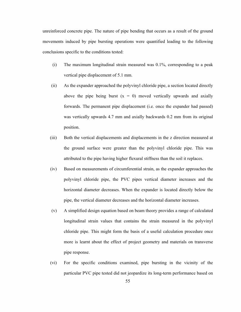
55

unreinforced concrete pipe. The nature of pipe bending that occurs as a result of the ground

movements induced by pipe bursting operations were quantified leading to the following

conclusions specific to the conditions tested:

(i) The maximum longitudinal strain measured was 0.1%, corresponding to a peak

vertical pipe displacement of 5.1 mm.

(ii) As the expander approached the polyvinyl chloride pipe, a section located directly

above the pipe being burst (x = 0) moved vertically upwards and axially

forwards. The permanent pipe displacement (i.e. once the expander had passed)

was vertically upwards 4.7 mm and axially backwards 0.2 mm from its original

position.

(iii) Both the vertical displacements and displacements in the z direction measured at

the ground surface were greater than the polyvinyl chloride pipe. This was

attributed to the pipe having higher flexural stiffness than the soil it replaces.

(iv) Based on measurements of circumferential strain, as the expander approaches the

polyvinyl chloride pipe, the PVC pipes vertical diameter increases and the

horizontal diameter decreases. When the expander is located directly below the

pipe, the vertical diameter decreases and the horizontal diameter increases.

(v) A simplified design equation based on beam theory provides a range of calculated

longitudinal strain values that contains the strain measured in the polyvinyl

chloride pipe. This might form the basis of a useful calculation procedure once

more is learnt about the effect of project geometry and materials on transverse

pipe response.

(vi) For the specific conditions examined, pipe bursting in the vicinity of the

particular PVC pipe tested did not jeopardize its long-term performance based on

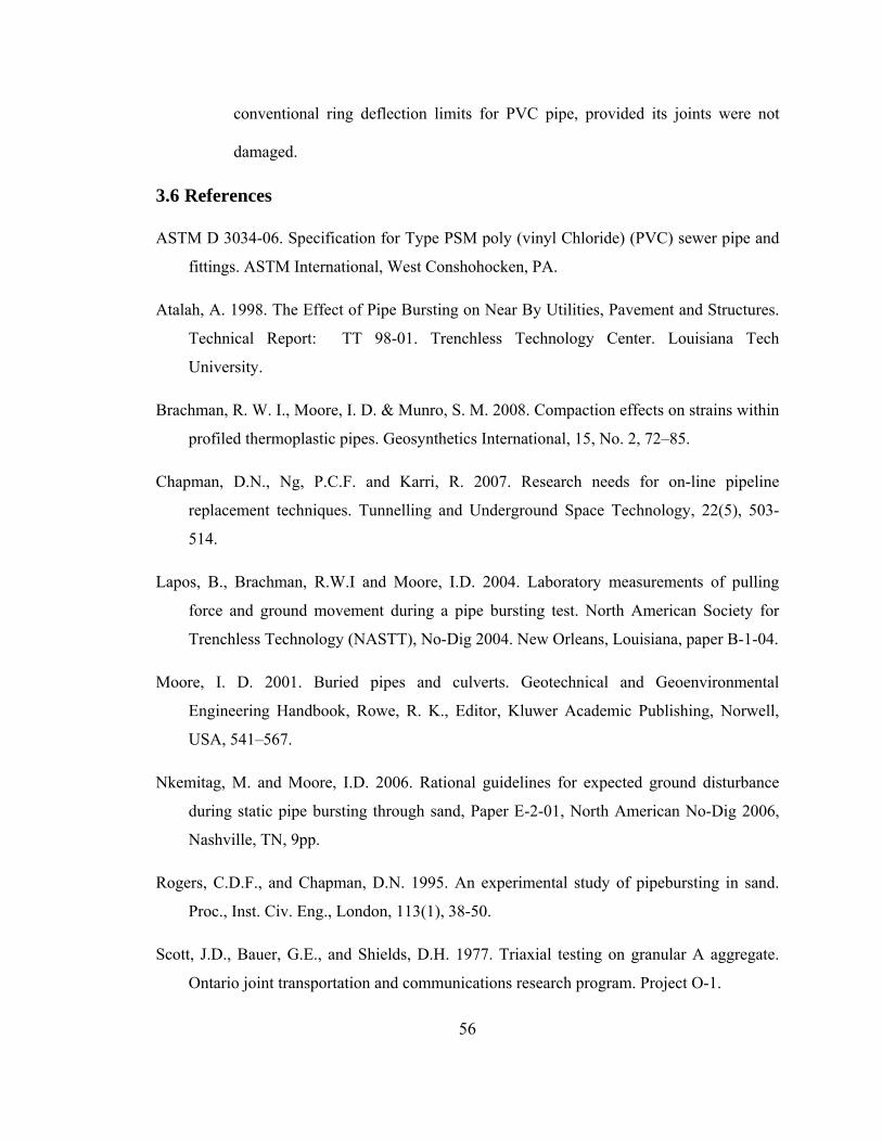
56

conventional ring deflection limits for PVC pipe, provided its joints were not

damaged.

3.6 References

ASTM D 3034-06. Specification for Type PSM poly (vinyl Chloride) (PVC) sewer pipe and

fittings. ASTM International, West Conshohocken, PA.

Atalah, A. 1998. The Effect of Pipe Bursting on Near By Utilities, Pavement and Structures.

Technical Report: TT 98-01. Trenchless Technology Center. Louisiana Tech

University.

Brachman, R. W. I., Moore, I. D. & Munro, S. M. 2008. Compaction effects on strains within

profiled thermoplastic pipes. Geosynthetics International, 15, No. 2, 72–85.

Chapman, D.N., Ng, P.C.F. and Karri, R. 2007. Research needs for on-line pipeline

replacement techniques. Tunnelling and Underground Space Technology, 22(5), 503-

514.

Lapos, B., Brachman, R.W.I and Moore, I.D. 2004. Laboratory measurements of pulling

force and ground movement during a pipe bursting test. North American Society for

Trenchless Technology (NASTT), No-Dig 2004. New Orleans, Louisiana, paper B-1-04.

Moore, I. D. 2001. Buried pipes and culverts. Geotechnical and Geoenvironmental

Engineering Handbook, Rowe, R. K., Editor, Kluwer Academic Publishing, Norwell,

USA, 541–567.

Nkemitag, M. and Moore, I.D. 2006. Rational guidelines for expected ground disturbance

during static pipe bursting through sand, Paper E-2-01, North American No-Dig 2006,

Nashville, TN, 9pp.

Rogers, C.D.F., and Chapman, D.N. 1995. An experimental study of pipebursting in sand.

Proc., Inst. Civ. Eng., London, 113(1), 38-50.

Scott, J.D., Bauer, G.E., and Shields, D.H. 1977. Triaxial testing on granular A aggregate.

Ontario joint transportation and communications research program. Project O-1.

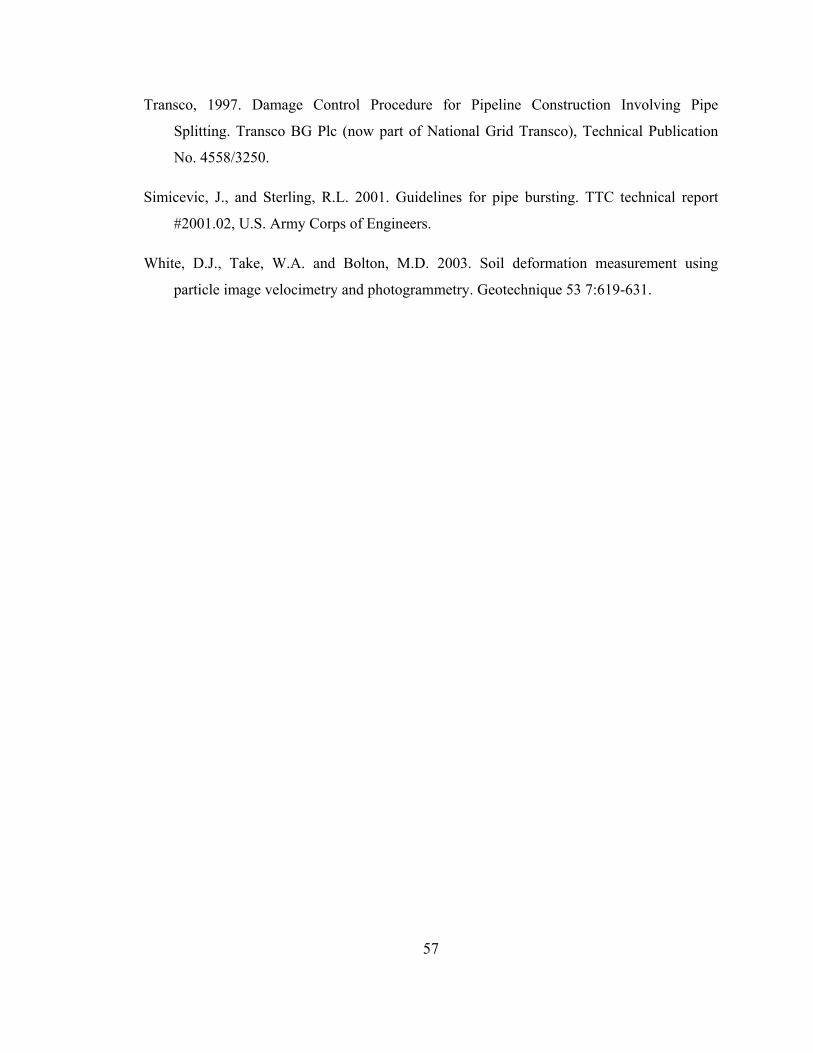
57

Transco, 1997. Damage Control Procedure for Pipeline Construction Involving Pipe

Splitting. Transco BG Plc (now part of National Grid Transco), Technical Publication

No. 4558/3250.

Simicevic, J., and Sterling, R.L. 2001. Guidelines for pipe bursting. TTC technical report

#2001.02, U.S. Army Corps of Engineers.

White, D.J., Take, W.A. and Bolton, M.D. 2003. Soil deformation measurement using

particle image velocimetry and photogrammetry. Geotechnique 53 7:619-631.

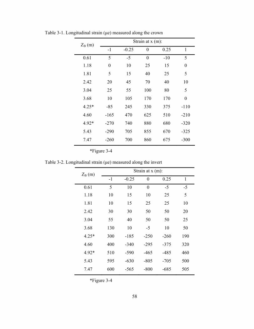
58

Table 3-1. Longitudinal strain (μe) measured along the crown

Strain at x (m): ZB (m)

-1 -0.25 0 0.25 1

0.61 5 -5 0 -10 5 1.18 0 10 25 15 0

1.81 5 15 40 25 5

2.42 20 45 70 40 10

3.04 25 55 100 80 5

3.68 10 105 170 170 0

4.25* -85 245 330 375 -110

4.60 -165 470 625 510 -210

4.92* -270 740 880 680 -320

5.43 -290 705 855 670 -325

7.47 -260 700 860 675 -300

*Figure 3-4 Table 3-2. Longitudinal strain (μe) measured along the invert

Strain at x (m): ZB (m)

-1 -0.25 0 0.25 1

0.61 5 10 0 -5 -5 1.18 10 15 10 25 5

1.81 10 15 25 25 10

2.42 30 30 50 50 20

3.04 55 40 50 50 25

3.68 130 10 -5 10 50

4.25* 300 -185 -250 -260 190

4.60 400 -340 -295 -375 320

4.92* 510 -590 -465 -485 460

5.43 595 -630 -805 -705 500

7.47 600 -565 -800 -685 505

*Figure 3-4

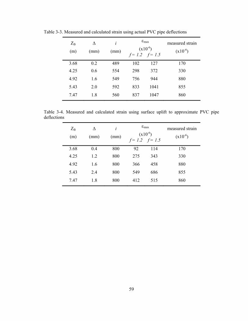
59

Table 3-3. Measured and calculated strain using actual PVC pipe deflections

εmax

(x10-6) ZB

(m)

Δ

(mm)

i

(mm) f = 1.2 f = 1.5

measured strain

(x10-6)

3.68 0.2 489 102 127 170 4.25 0.6 554 298 372 330

4.92 1.6 549 756 944 880

5.43 2.0 592 833 1041 855

7.47 1.8 560 837 1047 860

Table 3-4. Measured and calculated strain using surface uplift to approximate PVC pipe deflections

εmax

(x10-6) ZB

(m)

Δ

(mm)

i

(mm) f = 1.2 f = 1.5

measured strain

(x10-6)

3.68 0.4 800 92 114 170 4.25 1.2 800 275 343 330

4.92 1.6 800 366 458 880

5.43 2.4 800 549 686 855

7.47 1.8 800 412 515 860

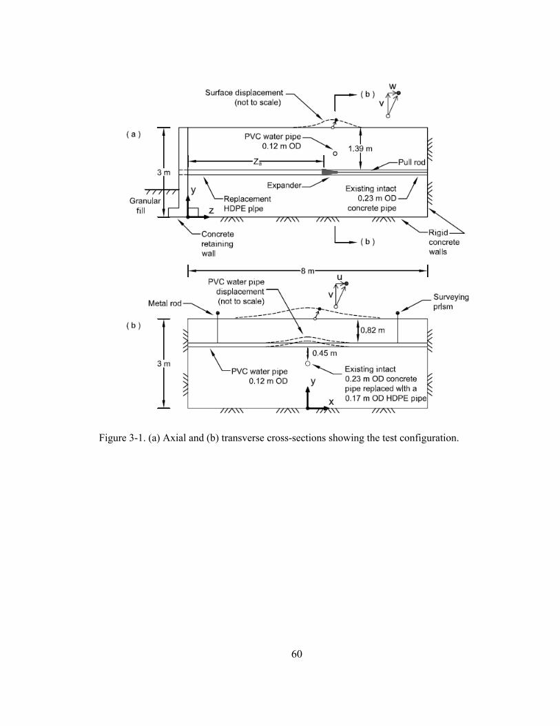
60

Figure 3-1. (a) Axial and (b) transverse cross-sections showing the test configuration.

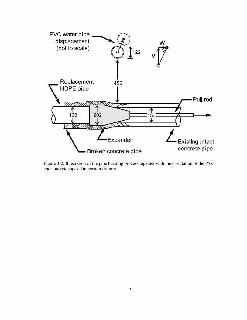
61

Figure 3-2. Illustration of the pipe bursting process together with the orientation of the PVC and concrete pipes. Dimensions in mm.

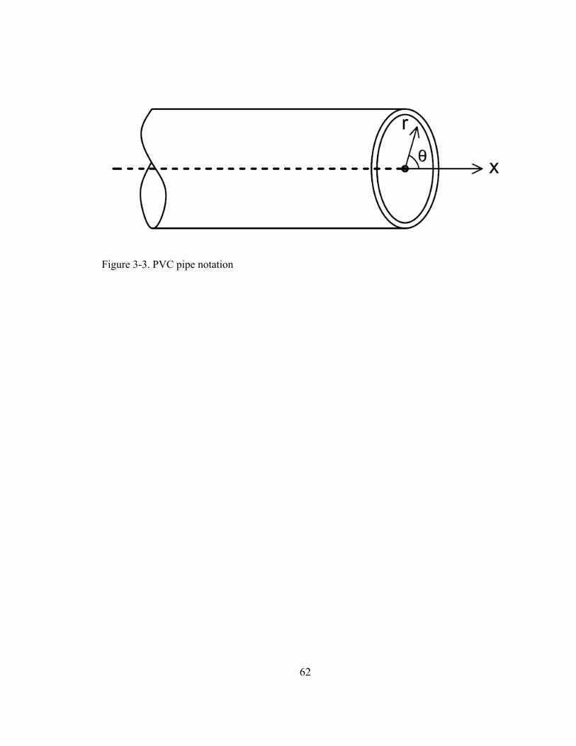
62

Figure 3-3. PVC pipe notation

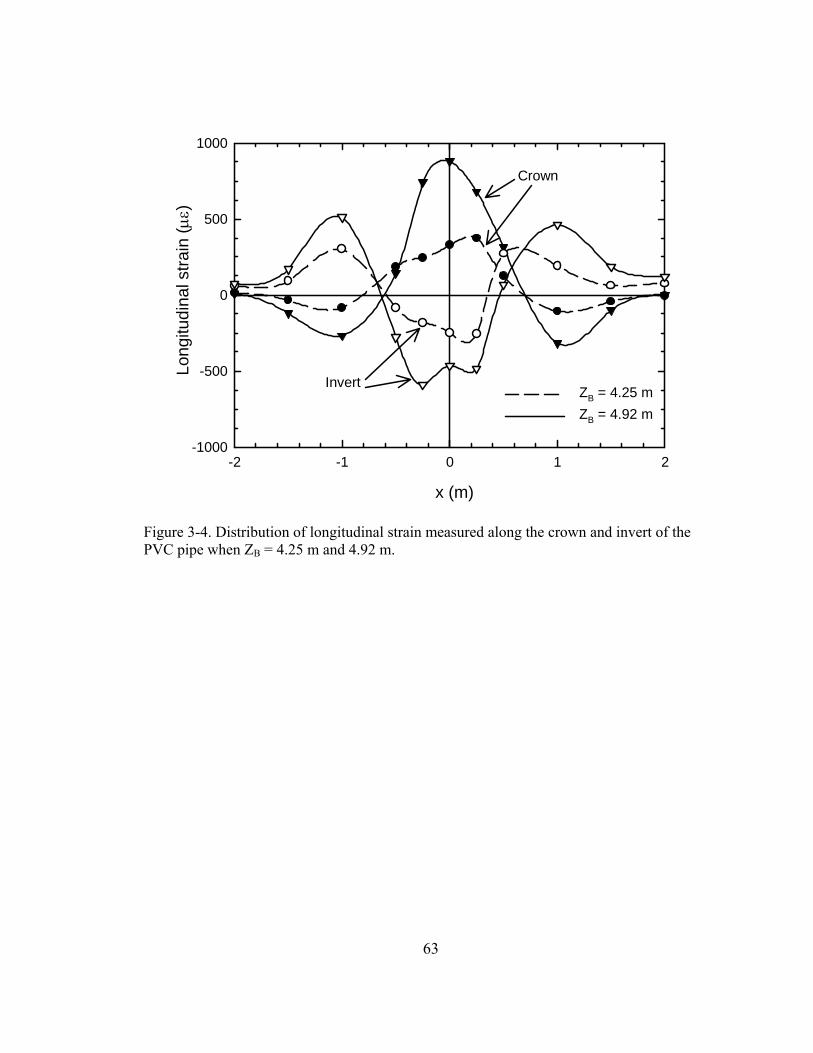
63

x (m)

-2 -1 0 1 2

Long

itudi

nal s

train

(με )

-1000

-500

0

500

1000

ZB = 4.25 mZB = 4.92 m

Crown

Invert

Figure 3-4. Distribution of longitudinal strain measured along the crown and invert of the PVC pipe when ZB = 4.25 m and 4.92 m.

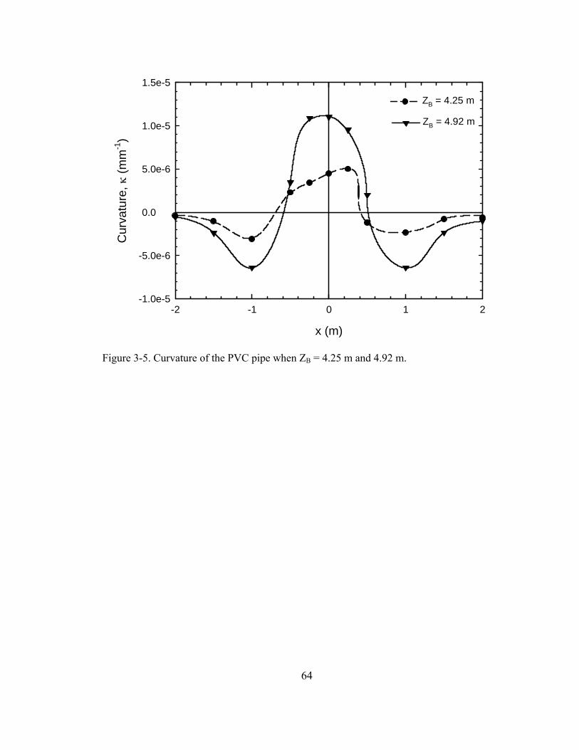
64

ZB = 4.92 m

ZB = 4.25 m

ZB = 4.92 m

ZB = 4.25 m

x (m)

-2 -1 0 1 2

Cur

vatu

re, κ

(mm

-1)

-1.0e-5

-5.0e-6

0.0

5.0e-6

1.0e-5

1.5e-5

Figure 3-5. Curvature of the PVC pipe when ZB = 4.25 m and 4.92 m.

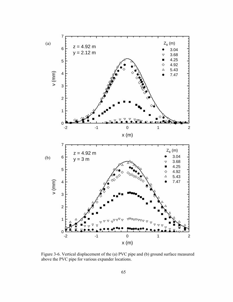
65

x (m)-2 -1 0 1 2

v (m

m)

7

6

5

4

3

2

1

0

3.043.684.254.925.437.47

ZB (m)z = 4.92 my = 2.12 m

x (m)-2 -1 0 1 2

v (m

m)

0

1

2

3

4

5

6

7

3.043.684.254.925.437.47

ZB (m)z = 4.92 my = 3 m

Figure 3-6. Vertical displacement of the (a) PVC pipe and (b) ground surface measured above the PVC pipe for various expander locations.

(a)

(b)

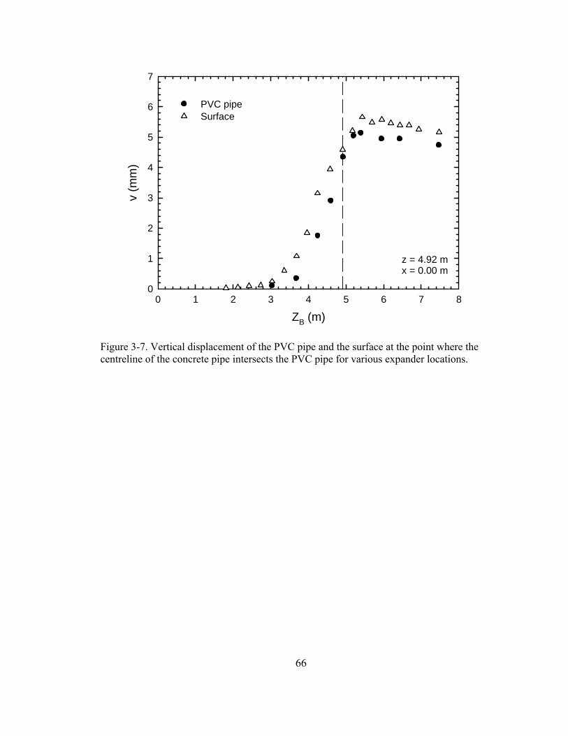
66

ZB (m)0 1 2 3 4 5 6 7 8

v (m

m)

0

1

2

3

4

5

6

7

PVC pipeSurface

z = 4.92 mx = 0.00 m

Figure 3-7. Vertical displacement of the PVC pipe and the surface at the point where the centreline of the concrete pipe intersects the PVC pipe for various expander locations.

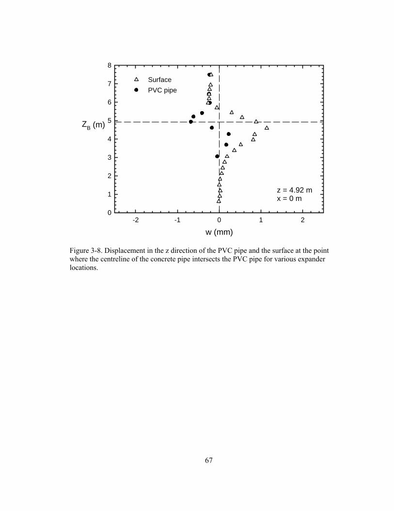
67

w (mm)-2 -1 0 1 2

ZB (m)

0

1

2

3

4

5

6

7

8

z = 4.92 mx = 0 m

SurfacePVC pipe

Figure 3-8. Displacement in the z direction of the PVC pipe and the surface at the point where the centreline of the concrete pipe intersects the PVC pipe for various expander locations.

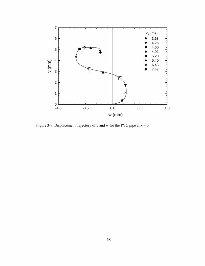
68

3.684.254.604.925.205.406.437.47

w (mm)-1.0 -0.5 0.0 0.5 1.0

v (m

m)

0

1

2

3

4

5

6

7ZB (m)

Figure 3-9. Displacement trajectory of v and w for the PVC pipe at x = 0.

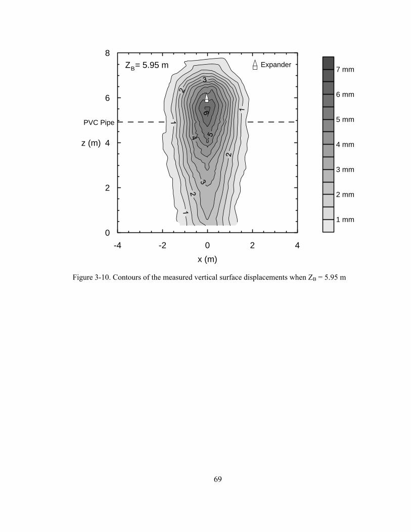
69

-4 -2 0 2 4x (m)

0

2

4

6

8

z (m)

1 mm

2 mm

3 mm

4 mm

5 mm

6 mm

7 mmZ = 5.95 mB Expander

PVC Pipe

Figure 3-10. Contours of the measured vertical surface displacements when ZB = 5.95 m

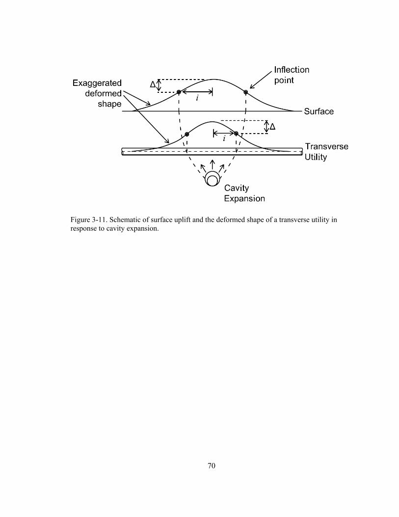
70

Figure 3-11. Schematic of surface uplift and the deformed shape of a transverse utility in response to cavity expansion.

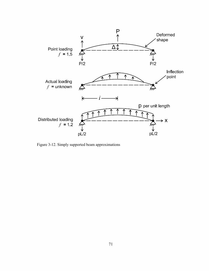
71

Figure 3-12. Simply supported beam approximations

72

Chapter 4

Axial stress-strain response of HDPE from whole pipe samples and

coupons

4.1 Introduction

Circumferential stresses and strains are generated in buried high density polyethylene

(HDPE) pipes due to gravity loading and, in the case of pressure pipes, the internal working

pressure. Pipes subjected to constant long-term stresses (i.e. those generated by the internal

working pressure in the pipe) may be prone to failure because of creep (strain accumulation

under constant stress) and slowly growing cracks in the semicrystalline structure of HDPE

(Mruk, 1990). Conversely, stresses in constantly deflected pipes will undergo stress

relaxation (stress dissipation under constant strain), which can be beneficial for the pipe. Pure

creep and stress relaxation experiments have been conducted using HDPE in the

circumferential direction by Mruk (1990) and Janson (1985), Chua and Lytton (1990), and

Hashash (1991) respectively.

However, under some circumstances HDPE pipes are subjected to axial stresses and

strains, such as during a pulled-in-place installation by horizontal directional drilling or pipe

bursting. Horizontal directional drilling involves pulling a new pipe through a borehole that is

created underground with a drill bit controlled from the ground surface (ASTM F1962).

During pipe bursting, an expander is pulled through an existing pipe, breaking it and forcing

the broken pipe fragments out into the surrounding soil. A new pipe is attached to the rear of

the expander and is pulled-into-place along the same trajectory as the existing pipe

(Simicevic and Sterling 2001). Creep and stress relaxation are prevalent conditions acting on

the HDPE pipe during and after installation using these types of techniques. Currently, there

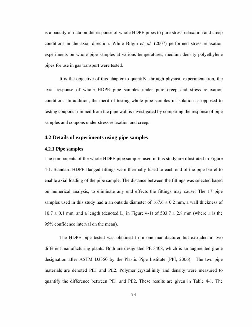
73

is a paucity of data on the response of whole HDPE pipes to pure stress relaxation and creep

conditions in the axial direction. While Bilgin et. al. (2007) performed stress relaxation

experiments on whole pipe samples at various temperatures, medium density polyethylene

pipes for use in gas transport were tested.

It is the objective of this chapter to quantify, through physical experimentation, the

axial response of whole HDPE pipe samples under pure creep and stress relaxation

conditions. In addition, the merit of testing whole pipe samples in isolation as opposed to

testing coupons trimmed from the pipe wall is investigated by comparing the response of pipe

samples and coupons under stress relaxation and creep.

4.2 Details of experiments using pipe samples

4.2.1 Pipe samples

The components of the whole HDPE pipe samples used in this study are illustrated in Figure

4-1. Standard HDPE flanged fittings were thermally fused to each end of the pipe barrel to

enable axial loading of the pipe sample. The distance between the fittings was selected based

on numerical analysis, to eliminate any end effects the fittings may cause. The 17 pipe

samples used in this study had a an outside diameter of 167.6 ± 0.2 mm, a wall thickness of

10.7 ± 0.1 mm, and a length (denoted Lo in Figure 4-1) of 503.7 ± 2.8 mm (where ± is the

95% confidence interval on the mean).

The HDPE pipe tested was obtained from one manufacturer but extruded in two

different manufacturing plants. Both are designated PE 3408, which is an augmented grade

designation after ASTM D3350 by the Plastic Pipe Institute (PPI, 2006). The two pipe

materials are denoted PE1 and PE2. Polymer crystallinity and density were measured to

quantify the difference between PE1 and PE2. These results are given in Table 4-1. The

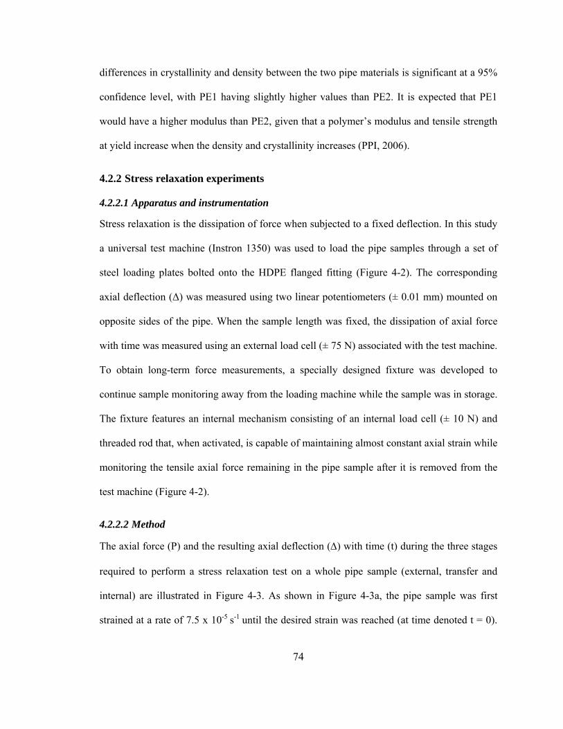
74

differences in crystallinity and density between the two pipe materials is significant at a 95%

confidence level, with PE1 having slightly higher values than PE2. It is expected that PE1

would have a higher modulus than PE2, given that a polymer’s modulus and tensile strength

at yield increase when the density and crystallinity increases (PPI, 2006).

4.2.2 Stress relaxation experiments

4.2.2.1 Apparatus and instrumentation

Stress relaxation is the dissipation of force when subjected to a fixed deflection. In this study

a universal test machine (Instron 1350) was used to load the pipe samples through a set of

steel loading plates bolted onto the HDPE flanged fitting (Figure 4-2). The corresponding

axial deflection (Δ) was measured using two linear potentiometers (± 0.01 mm) mounted on

opposite sides of the pipe. When the sample length was fixed, the dissipation of axial force

with time was measured using an external load cell (± 75 N) associated with the test machine.

To obtain long-term force measurements, a specially designed fixture was developed to

continue sample monitoring away from the loading machine while the sample was in storage.

The fixture features an internal mechanism consisting of an internal load cell (± 10 N) and

threaded rod that, when activated, is capable of maintaining almost constant axial strain while

monitoring the tensile axial force remaining in the pipe sample after it is removed from the

test machine (Figure 4-2).

4.2.2.2 Method

The axial force (P) and the resulting axial deflection (Δ) with time (t) during the three stages

required to perform a stress relaxation test on a whole pipe sample (external, transfer and

internal) are illustrated in Figure 4-3. As shown in Figure 4-3a, the pipe sample was first

strained at a rate of 7.5 x 10-5 s-1

until the desired strain was reached (at time denoted t = 0).

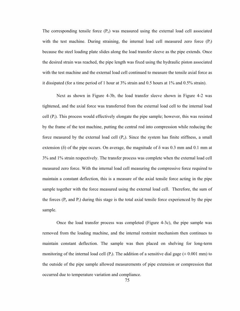
75

The corresponding tensile force (Pe) was measured using the external load cell associated

with the test machine. During straining, the internal load cell measured zero force (Pi)

because the steel loading plate slides along the load transfer sleeve as the pipe extends. Once

the desired strain was reached, the pipe length was fixed using the hydraulic piston associated

with the test machine and the external load cell continued to measure the tensile axial force as

it dissipated (for a time period of 1 hour at 3% strain and 0.5 hours at 1% and 0.5% strain).

Next as shown in Figure 4-3b, the load transfer sleeve shown in Figure 4-2 was

tightened, and the axial force was transferred from the external load cell to the internal load

cell (Pi). This process would effectively elongate the pipe sample; however, this was resisted

by the frame of the test machine, putting the central rod into compression while reducing the

force measured by the external load cell (Pe). Since the system has finite stiffness, a small

extension (δ) of the pipe occurs. On average, the magnitude of δ was 0.3 mm and 0.1 mm at

3% and 1% strain respectively. The transfer process was complete when the external load cell

measured zero force. With the internal load cell measuring the compressive force required to

maintain a constant deflection, this is a measure of the axial tensile force acting in the pipe

sample together with the force measured using the external load cell. Therefore, the sum of

the forces (Pe and Pi) during this stage is the total axial tensile force experienced by the pipe

sample.

Once the load transfer process was completed (Figure 4-3c), the pipe sample was

removed from the loading machine, and the internal restraint mechanism then continues to

maintain constant deflection. The sample was then placed on shelving for long-term

monitoring of the internal load cell (Pi). The addition of a sensitive dial gage (± 0.001 mm) to

the outside of the pipe sample allowed measurements of pipe extension or compression that

occurred due to temperature variation and compliance.

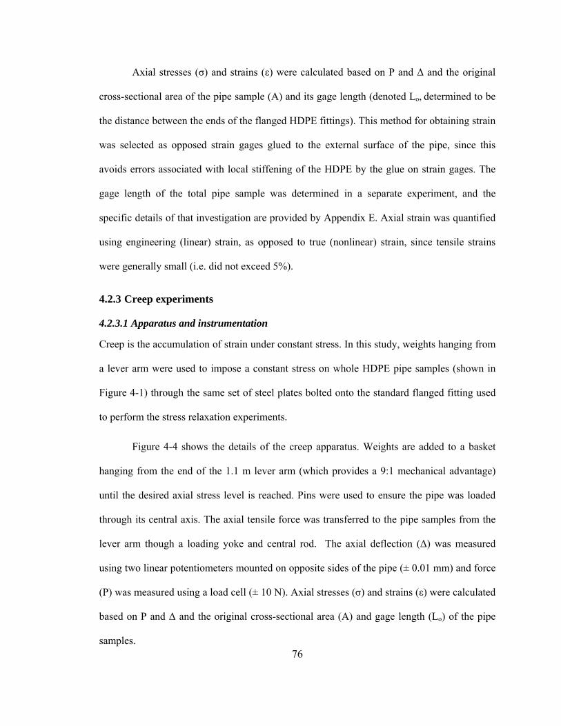
76

Axial stresses (σ) and strains (ε) were calculated based on P and Δ and the original

cross-sectional area of the pipe sample (A) and its gage length (denoted Lo, determined to be

the distance between the ends of the flanged HDPE fittings). This method for obtaining strain

was selected as opposed strain gages glued to the external surface of the pipe, since this

avoids errors associated with local stiffening of the HDPE by the glue on strain gages. The

gage length of the total pipe sample was determined in a separate experiment, and the

specific details of that investigation are provided by Appendix E. Axial strain was quantified

using engineering (linear) strain, as opposed to true (nonlinear) strain, since tensile strains

were generally small (i.e. did not exceed 5%).

4.2.3 Creep experiments

4.2.3.1 Apparatus and instrumentation

Creep is the accumulation of strain under constant stress. In this study, weights hanging from

a lever arm were used to impose a constant stress on whole HDPE pipe samples (shown in

Figure 4-1) through the same set of steel plates bolted onto the standard flanged fitting used

to perform the stress relaxation experiments.

Figure 4-4 shows the details of the creep apparatus. Weights are added to a basket

hanging from the end of the 1.1 m lever arm (which provides a 9:1 mechanical advantage)

until the desired axial stress level is reached. Pins were used to ensure the pipe was loaded

through its central axis. The axial tensile force was transferred to the pipe samples from the

lever arm though a loading yoke and central rod. The axial deflection (Δ) was measured

using two linear potentiometers mounted on opposite sides of the pipe (± 0.01 mm) and force

(P) was measured using a load cell (± 10 N). Axial stresses (σ) and strains (ε) were calculated

based on P and Δ and the original cross-sectional area (A) and gage length (Lo) of the pipe

samples.

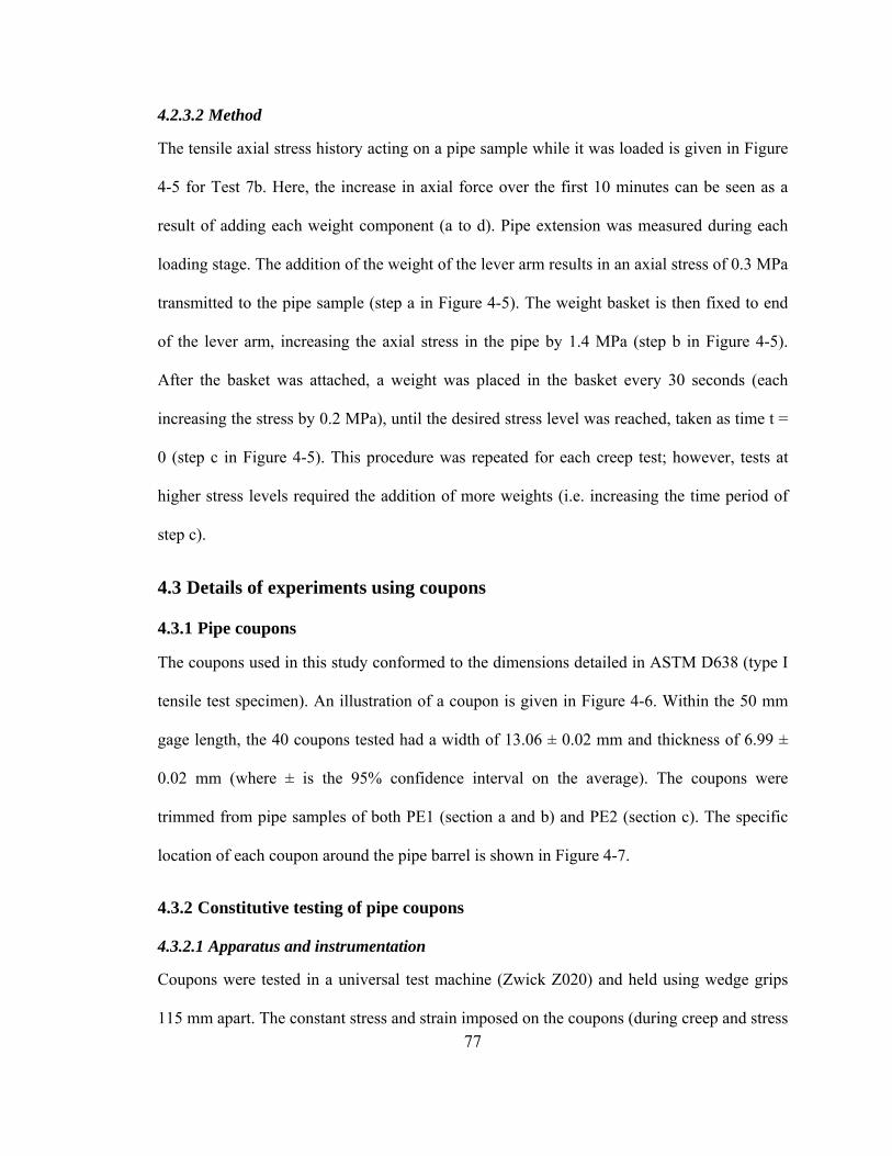
77

4.2.3.2 Method

The tensile axial stress history acting on a pipe sample while it was loaded is given in Figure

4-5 for Test 7b. Here, the increase in axial force over the first 10 minutes can be seen as a

result of adding each weight component (a to d). Pipe extension was measured during each

loading stage. The addition of the weight of the lever arm results in an axial stress of 0.3 MPa

transmitted to the pipe sample (step a in Figure 4-5). The weight basket is then fixed to end

of the lever arm, increasing the axial stress in the pipe by 1.4 MPa (step b in Figure 4-5).

After the basket was attached, a weight was placed in the basket every 30 seconds (each

increasing the stress by 0.2 MPa), until the desired stress level was reached, taken as time t =

0 (step c in Figure 4-5). This procedure was repeated for each creep test; however, tests at

higher stress levels required the addition of more weights (i.e. increasing the time period of

step c).

4.3 Details of experiments using coupons

4.3.1 Pipe coupons

The coupons used in this study conformed to the dimensions detailed in ASTM D638 (type I

tensile test specimen). An illustration of a coupon is given in Figure 4-6. Within the 50 mm

gage length, the 40 coupons tested had a width of 13.06 ± 0.02 mm and thickness of 6.99 ±

0.02 mm (where ± is the 95% confidence interval on the average). The coupons were

trimmed from pipe samples of both PE1 (section a and b) and PE2 (section c). The specific

location of each coupon around the pipe barrel is shown in Figure 4-7.

4.3.2 Constitutive testing of pipe coupons

4.3.2.1 Apparatus and instrumentation

Coupons were tested in a universal test machine (Zwick Z020) and held using wedge grips

115 mm apart. The constant stress and strain imposed on the coupons (during creep and stress

78

relaxation testing respectively) were the same magnitude as those imposed on the whole pipe

samples. The deflection, over the 50 mm gage length, was measured and controlled using a

clip-on extensometer (± 0.005 mm), and the force was measured and controlled by a load cell

associated with the test machine (± 0.1 N). Axial stresses (σ) and strains (ε) were calculated

based on P and Δ and the coupons original cross-sectional area (A) and gage length (50 mm).

4.3.2.2 Method

The three types of experiments performed on the coupons included: stress relaxation, creep,

and a strain controlled load path featuring two unload-reload cycles. The coupons used for

stress relaxation testing were strained at a rate of 7.5 x 10-5 s-1

until the desired strain

magnitude was reached (an identical strain rate to that used on the pipe samples). Creep

experiments on coupons were conducted following the procedure detailed in ASTM D2990;

however, the procedure was slightly modified, so the same stress history imposed on the

whole pipe samples was used for the coupons (Figure 4-5). In addition to the stress relaxation

and creep experiments, a third test was performed only on the coupons, which involved a

strain controlled load path. It was adopted to include unload-reload cycles within and beyond

the elastic region as well as loading up to and beyond the yield point. The load path was

performed at a strain rate of 7.5 x 10-5 s-1, and featured two unload-reload cycles at 1% and

5% strain (unloading to 0.8% and 4% respectively), before loading continued up to a

maximum strain of 25%.

4.4 Tests conducted

In general, creep and stress relaxation experiments performed on the pipe samples and

coupons were completed in triplicate, to assess the repeatability of the results. For each

loading condition, one pipe sample was tested up to 1000 hours while the other two were

79

tested to 100 hours. Coupons were tested for shorter time periods, one up to 100 hours and

the others for 10 hours. Most of the experiments performed in this study involved testing

PE1. Tests 4 and 46 through 50 were conducted on PE2.

Details of the stress relaxation experiments performed are given in Table 4-2. Stress

relaxation experiments were performed on pipe samples and repeated on coupons at strain

levels of 3% (Test 3 and Test 6) and 1% (Test 2 and Test 5). In addition, pipe samples were

tested at 0.5% (Test 1) and 1% strain using PE2 (Test 4). A summary of the creep

experiments performed is provided in Table 4-3. Pipes and coupons were tested at stress

levels of 8 MPa (Tests 8 and 10) and 4 MPa (Tests 7 and 9). Details of the twenty-nine strain

controlled load path experiments performed on the coupons are given in Table 4-4. All

experiments were performed at room temperature (i.e. from 21°C to 23°C).

4.5 Results

4.5.1 Stress relaxation

Results from stress relaxation experiments performed on whole pipe samples at 0.5% (Test

1a), 1% (Test 2a and 4c), and 3% (Test 3c) strain and coupons at 1% (Test 5b) and 3% (Test

6a) strain are given in Figure 4-8. A summary of the results, for these and all the other stress

relaxation tests, is given in Table 4-2. The minor spike in axial stress in the pipe samples

(after 0.5 hours during Tests 1a, 2a, and 4c and after 1 hour during Test 3c) can be attributed

to the load transfer process. It does not appear to affect the subsequent stress relaxation

results (i.e. the slope of the relaxation curve is similar before and immediately after the

transfer). The results in Figure 4-8 show the dissipation (or relaxation) of axial stresses in the

pipe samples and coupons when a constant strain condition is imposed. When a pipe sample

was subjected to 3% strain (Test 3c), the initial stress in the sample (at t = 0) was 12.0 MPa

80

(σ0), and this relaxed to 8.2 MPa (σ1), 6.8 MPa (σ10), and 6.1 MPa (σ100) after 1 hour, 10

hours, and 100 hours respectively. On average (in Tests 1, 2, and 3), 63% of the initial stress

remained in the pipes samples after 1 hour (σ1 divided by σ0), decreasing to 55%, 49%, and

43% after 10 hours, 100 hours, and 1000 hours respectively.

At identical strain rates, the magnitude of σ0 was generally greater in the coupons

than in the pipe samples. This suggests that the coupons have a higher modulus (i.e. a greater

stress is required to reach the same strain) than the pipe samples even though the same

material was tested (PE1). In fact, Figure 4-9 shows the ratio of stresses observed in the pipe

samples and coupons during the stress relaxation tests at 1% (Tests 2a and 5b) and 3% (Tests

3c and 6a) strain. During relaxation, the magnitude of axial stress remaining in the coupons

was generally 1.1 and 1.03 times greater than the pipe samples at 1% and 3% respectively.

Stresses dissipated slightly more quickly in the pipe sample. For instance, in the coupons (in

Tests 5 and 6) 66%, 56%, and 51% of the initial stress remained after 1 hour, 10 hours, and

100 hours respectively, as opposed to 63%, 55%, and 49% of the stress which remained in

the pipe samples (in Tests 1, 2, and 3).

An additional stress relaxation experiment at 1% strain was performed on pipe

samples made from PE2 in Test 4. Values of σ0, σ1, σ10, and σ100 were all less for the pipe

sample made from the pipe material designated PE2 (Test 4c), than those seen in a similar

test performed on PE1 (Test 2a) as shown in Figure 4-8. This indicates that PE1 had a higher

modulus than PE2. Stresses in pipe samples made from PE2 relaxed somewhat more quickly

than pipe samples made from PE1. Pipe samples made from PE2 (Test 4) on average had

61%, 54%, and 46% of the initial stress remaining after 1 hour, 10 hours, and 100 hours

respectively, as opposed to proportions 63%, 55%, and 48% which remained in the pipe

samples made from PE1 (Test 2).

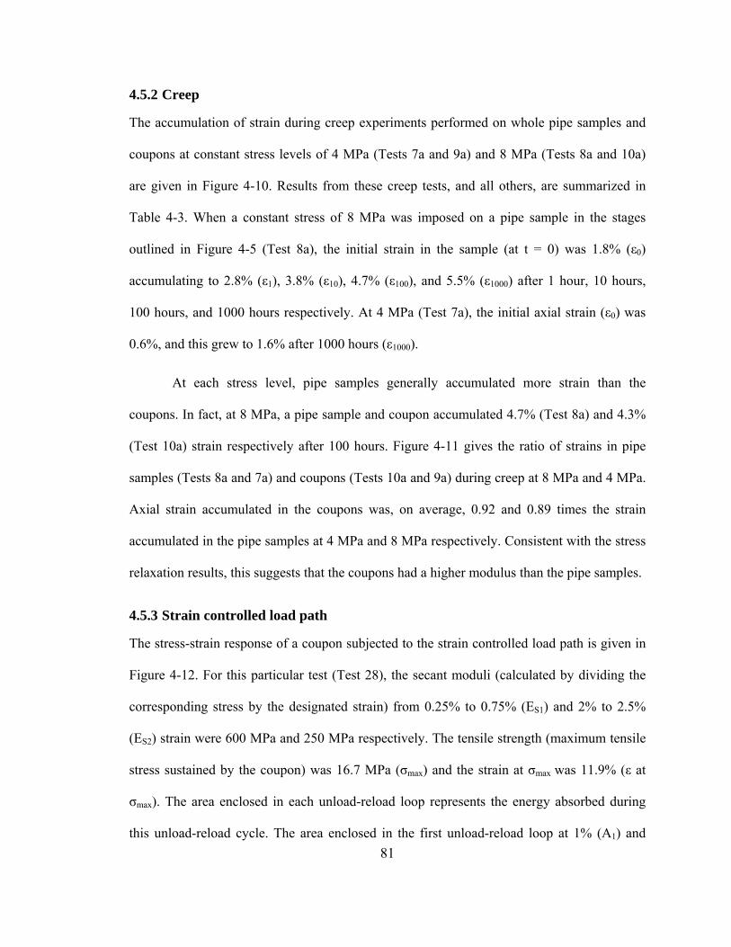
81

4.5.2 Creep

The accumulation of strain during creep experiments performed on whole pipe samples and

coupons at constant stress levels of 4 MPa (Tests 7a and 9a) and 8 MPa (Tests 8a and 10a)

are given in Figure 4-10. Results from these creep tests, and all others, are summarized in

Table 4-3. When a constant stress of 8 MPa was imposed on a pipe sample in the stages

outlined in Figure 4-5 (Test 8a), the initial strain in the sample (at t = 0) was 1.8% (ε0)

accumulating to 2.8% (ε1), 3.8% (ε10), 4.7% (ε100), and 5.5% (ε1000) after 1 hour, 10 hours,

100 hours, and 1000 hours respectively. At 4 MPa (Test 7a), the initial axial strain (ε0) was

0.6%, and this grew to 1.6% after 1000 hours (ε1000).

At each stress level, pipe samples generally accumulated more strain than the

coupons. In fact, at 8 MPa, a pipe sample and coupon accumulated 4.7% (Test 8a) and 4.3%

(Test 10a) strain respectively after 100 hours. Figure 4-11 gives the ratio of strains in pipe

samples (Tests 8a and 7a) and coupons (Tests 10a and 9a) during creep at 8 MPa and 4 MPa.

Axial strain accumulated in the coupons was, on average, 0.92 and 0.89 times the strain

accumulated in the pipe samples at 4 MPa and 8 MPa respectively. Consistent with the stress

relaxation results, this suggests that the coupons had a higher modulus than the pipe samples.

4.5.3 Strain controlled load path

The stress-strain response of a coupon subjected to the strain controlled load path is given in

Figure 4-12. For this particular test (Test 28), the secant moduli (calculated by dividing the

corresponding stress by the designated strain) from 0.25% to 0.75% (ES1) and 2% to 2.5%

(ES2) strain were 600 MPa and 250 MPa respectively. The tensile strength (maximum tensile

stress sustained by the coupon) was 16.7 MPa (σmax) and the strain at σmax was 11.9% (ε at

σmax). The area enclosed in each unload-reload loop represents the energy absorbed during

this unload-reload cycle. The area enclosed in the first unload-reload loop at 1% (A1) and

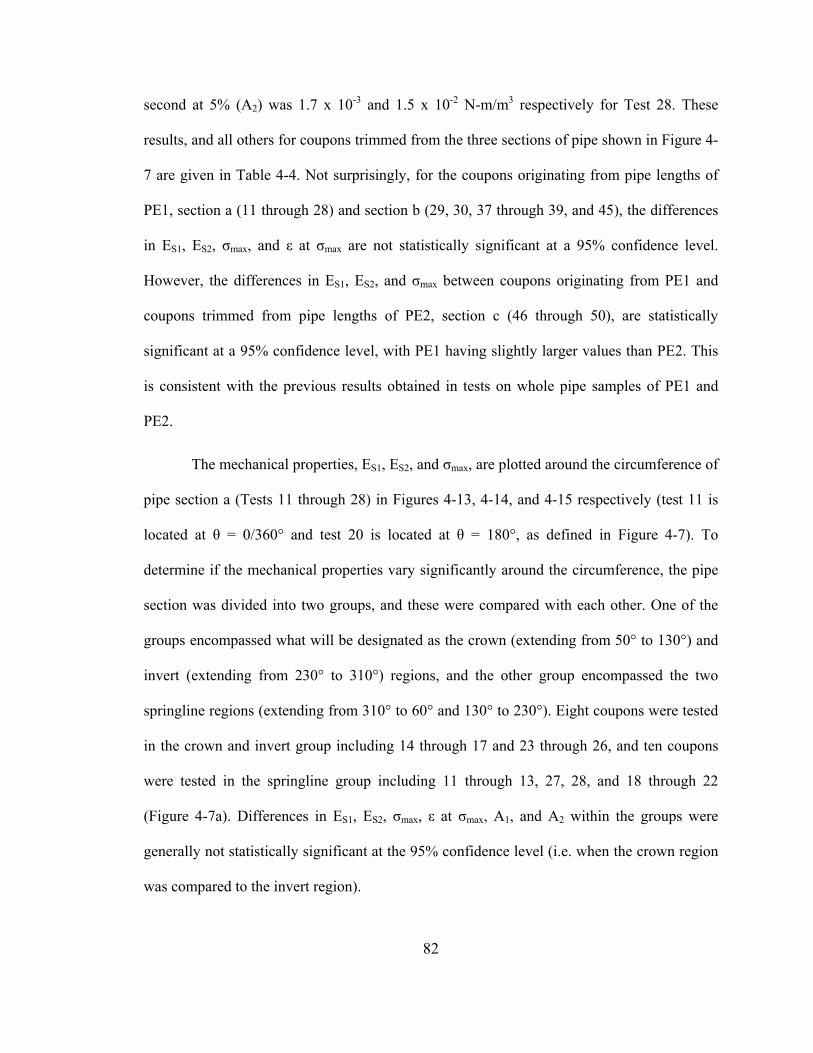
82

second at 5% (A2) was 1.7 x 10-3 and 1.5 x 10-2 N-m/m3 respectively for Test 28. These

results, and all others for coupons trimmed from the three sections of pipe shown in Figure 4-

7 are given in Table 4-4. Not surprisingly, for the coupons originating from pipe lengths of

PE1, section a (11 through 28) and section b (29, 30, 37 through 39, and 45), the differences

in ES1, ES2, σmax, and ε at σmax are not statistically significant at a 95% confidence level.

However, the differences in ES1, ES2, and σmax between coupons originating from PE1 and

coupons trimmed from pipe lengths of PE2, section c (46 through 50), are statistically

significant at a 95% confidence level, with PE1 having slightly larger values than PE2. This

is consistent with the previous results obtained in tests on whole pipe samples of PE1 and

PE2.

The mechanical properties, ES1, ES2, and σmax, are plotted around the circumference of

pipe section a (Tests 11 through 28) in Figures 4-13, 4-14, and 4-15 respectively (test 11 is

located at θ = 0/360° and test 20 is located at θ = 180°, as defined in Figure 4-7). To

determine if the mechanical properties vary significantly around the circumference, the pipe

section was divided into two groups, and these were compared with each other. One of the

groups encompassed what will be designated as the crown (extending from 50° to 130°) and

invert (extending from 230° to 310°) regions, and the other group encompassed the two

springline regions (extending from 310° to 60° and 130° to 230°). Eight coupons were tested

in the crown and invert group including 14 through 17 and 23 through 26, and ten coupons

were tested in the springline group including 11 through 13, 27, 28, and 18 through 22

(Figure 4-7a). Differences in ES1, ES2, σmax, ε at σmax, A1, and A2 within the groups were

generally not statistically significant at the 95% confidence level (i.e. when the crown region

was compared to the invert region).

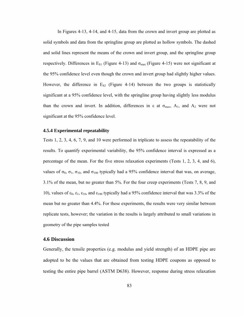
83

In Figures 4-13, 4-14, and 4-15, data from the crown and invert group are plotted as

solid symbols and data from the springline group are plotted as hollow symbols. The dashed

and solid lines represent the means of the crown and invert group, and the springline group

respectively. Differences in ES1 (Figure 4-13) and σmax (Figure 4-15) were not significant at

the 95% confidence level even though the crown and invert group had slightly higher values.

However, the difference in ES2 (Figure 4-14) between the two groups is statistically

significant at a 95% confidence level, with the springline group having slightly less modulus

than the crown and invert. In addition, differences in ε at σmax, A1, and A2 were not

significant at the 95% confidence level.

4.5.4 Experimental repeatability

Tests 1, 2, 3, 4, 6, 7, 9, and 10 were performed in triplicate to assess the repeatability of the

results. To quantify experimental variability, the 95% confidence interval is expressed as a

percentage of the mean. For the five stress relaxation experiments (Tests 1, 2, 3, 4, and 6),

values of σ0, σ1, σ10, and σ100 typically had a 95% confidence interval that was, on average,

3.1% of the mean, but no greater than 5%. For the four creep experiments (Tests 7, 8, 9, and

10), values of ε0, ε1, ε10, and ε100 typically had a 95% confidence interval that was 3.3% of the

mean but no greater than 4.4%. For these experiments, the results were very similar between

replicate tests, however; the variation in the results is largely attributed to small variations in

geometry of the pipe samples tested

4.6 Discussion

Generally, the tensile properties (e.g. modulus and yield strength) of an HDPE pipe are

adopted to be the values that are obtained from testing HDPE coupons as opposed to

testing the entire pipe barrel (ASTM D638). However, response during stress relaxation

84

and creep conditions for coupons trimmed from the barrel of a pipe was different to

results from tests on the complete pipe barrel. In fact, the coupons appeared to exhibit a

higher modulus than the whole pipe samples. The cause for this apparent increase in

modulus that occurs in HDPE when a coupon is trimmed from a pipe wall is unclear;

however, it may be attributed to release of the residual stresses generated during the

extrusion process, used to manufacture the pipes. Now, a tension test performed on a

coupon will give the tensile properties at a specific location around the pipe

circumference (i.e. at the location of that coupon), whereas tension testing of the whole

pipe sample will give the average tensile properties over the entire pipe barrel. However,

it was shown that the variation in the tensile properties (ES1, σmax, ε at σmax, A1, and A2)

around the circumference of a pipe was not statistically significant at the 95% confidence

level. Only ES2 varied in any statistically significant way, and this supports the hypothesis

that residual stress may be involved, since residual stresses would be expected to change

the modulus at higher levels of stress. This suggests that the only benefit gained from

testing whole pipe samples would be to eliminate any release of residual stresses when

coupons are machined from the pipe wall. This benefit is often overshadowed by the

relative ease in which experiments on coupons can be conducted compared to the

complexities that arise when testing a whole pipe sample. However, because the whole

pipe barrel is subjected to axial tensile stresses and strains during an actual HDD

installation, the whole pipe will be tested to investigate HDPE response during HDD in

Chapter 5.

85

4.7 Conclusions

Experimental results from a laboratory investigation into the constitutive properties HDPE

using both whole pipe samples and specimens trimmed from a pipe’s wall are presented. The

experiments conducted include creep, stress relaxation, and a strain controlled load path

featuring two unload-reload cycles. HDPE response to stress relaxation and creep conditions

and the merits of testing whole pipe samples were investigated leading to the following

conclusions for the particular materials and conditions tested:

(i) During stress relaxation experiments performed on whole HDPE pipe samples,

60% of the axial stress remained in the pipe samples after 1 hour of relaxation;

and after 1000 hours just 40% remained (on average).

(ii) Whole pipe samples subjected to sustained stresses of 4 MPa and 8 MPa

accumulated strain values of 1.6% and 5.5% respectively after 1000 hours.

(iii) Two types of HDPE pipe samples manufactured on different production lines

exhibited different moduli, highlighting the influence of crystallinity and density

on the constitutive properties of HDPE.

(iv) Results from identical stress relaxation and creep tests performed on the whole

pipe samples and coupons were compared, and these demonstrated that the

coupons exhibited higher modulus than the pipe samples. The apparent increase

in modulus of HDPE when specimens are trimmed from a pipe wall may be

attributed to the release of residual stresses.

(v) Coupons trimmed from 18 locations around the circumference of a pipe were

tested. The secant modulus from 0.25% to 0.75%, maximum tensile stress,

elongation at maximum tensile stress, and the area enclosed in the unload-reload

loops did not differ significantly around the circumference. However, the secant

86

modulus from 2% to 2.5% did differ significantly at the 95% confidence level

between the locations designated as the crown and invert, and the springlines.

(vi) The benefit of testing whole pipe samples as opposed to simply testing coupons

trimmed from a pipe wall is often overshadowed by the relative ease in which

experiments on coupons can be conducted compared to the complexities that arise

when testing a whole pipe sample.

4.8 References

ASTM D 638-03. Standard Test Method for Tensile Properties of Plastics. ASTM

International, West Conshohocken, PA.

ASTM E 794-95. Standard Test Method for Melting and Crystallization Temperatures by

Thermal Analysis. ASTM International, West Conshohocken, PA.

ASTM D 1238. Standard Test Method for Melt Flow Rates of Thermoplastics by Extrusion

Plastometer. ASTM International, West Conshohocken, PA.

ASTM D 1505-03. Standard Test Method for Density of Plastics by the Density-Gradient

Technique. ASTM International, West Conshohocken, PA.

ASTM F 1962-05 Standard Guide for Use of Maxi-Horizontal Directional Drilling for

Placement of Polyethylene Pipe or Conduit Under Obstacles, Including River Crossings.

ASTM International, West Conshohocken, PA.

ASTM E 794-95. Standard Test Method for Melting and Crystallization Temperatures by

Thermal Analysis. ASTM International, West Conshohocken, PA.

ASTM D 2990-01. Standard Test Methods for Tensile, Compressive, and Flexural Creep and

Creep-Rupture of Plastics. ASTM International, West Conshohocken, PA.

ASTM D 3350-08. Standard Specification for Polyethylene Plastics Pipe and Fittings

Materials. ASTM International, West Conshohocken, PA.

87

Bilgin, O, Stewart, H.E. and O’Rourke, T.D. 2007. Thermal and mechanical properties of

polyethylene pipes. Journal of Materials in Civil Engineering, 19(12), 1043-1052

Chua, K. M., and Lytton, R. L. 1990. Viscoelastic approach to modeling performance of

buried pipes. Journal of Transportation Engineering, 115(3), 253–269.

Hashash, N. M. 1991. Design and analysis of deeply buried polyethylene drainage pipes.

Ph.D. dissertation, Univ. of Massachusetts, Amherst, Mass.

Janson, L. 1985. Investigation of the long-term creep modulus for buried polyethylene

pipes subjected to constant deflection, Advances in Underground Pipeline Engineering

Proceedings of the International Conference, ACSE: 253-262.

Mruk, S.A. 1990. The durability of polyethylene piping, Buried Plastic Pipe Technology.

ASTM STP 1093, G.S. Buczala and M.J. Cassady (Eds.) ASCE, pp 21-39

PPI Handbook of Polyethylene Pipe, 1st ed., 2006. pp 47-156. Plastic Pipe Institute, Irving,

TX.

Simicevic, J., and Sterling, R.L. 2001. Guidelines for pipe bursting. TTC technical report

#2001.02, U.S. Army Corps of Engineers.

White, D.J., Take, W.A. & Bolton, M.D. 2003. Soil deformation measurement using particle

image velocimetry and photogrammetry. Geotechnique 53 7:619-631.

88

Table 4-1. Index properties (mean ± 95% confidence interval) for PE1 and PE2

Property Test Method PE1 PE2

Density (g/cm3) ASTM D1505 0.955 (± 0.002) 0.951 (± 0.001)

Crystallinity (%) ASTM E794 52.4 (± 1.15) 48.7 (± 1.97) Table 4-2. Stress relaxation test summary and results

Test Strain (%) Type PE Temp

(°C) σ0

(MPa) σ1

(MPa) σ10

(MPa) σ100

(MPa) σ1000

(MPa)

1a 0.5 Pipe 1 24.2 ± 0.2 4.1 2.4 2.0 1.9 1.7 1b 0.5 Pipe 1 22.1 ± 0.1 4.3 2.6 2.4 2.0 - 1c 0.5 Pipe 1 22.1 ± 0.1 4.3 2.6 2.3 2.1 - 2a 1 Pipe 1 23.4 ± 0.8 6.6 4.2 3.8 3.3 2.8 2b 1 Pipe 1 21.8 ± 0.2 6.7 4.2 3.6 3.2 - 2c 1 Pipe 1 22.1 ± 0.1 6.8 4.2 3.6 3.2 - 3a 3 Pipe 1 24.2 ± 0.2 12.3 8.5 7.5 6.8 6.1 3b 3 Pipe 1 21.8 ± 0.2 12.0 7.8 6.8 6.1 - 3c 3 Pipe 1 22.1 ± 0.1 12.0 8.2 6.8 6.1 - 4a 1 Pipe 2 23.0 ± 0.3 6.1 3.7 3.3 2.9 - 4b 1 Pipe 2 22.7 ± 0.3 6.3 3.6 3.3 2.8 - 4c 1 Pipe 2 22.7 ± 0.3 6.0 3.8 3.3 2.8 - 5a 1 Coupon 1 23.2 ± 0.1 6.9 4.6 3.9 - - 5b 1 Coupon 1 23.5 ± 0.1 7.2 4.7 3.9 - - 6a 3 Coupon 1 22.9 ± 0.7 12.4 8.2 7.0 6.3 - 6b 3 Coupon 1 23.2 ± 0.2 12.1 8.1 6.9 - - 6c 3 Coupon 1 21.3 ± 0.1 12.5 8.5 7.1 - -

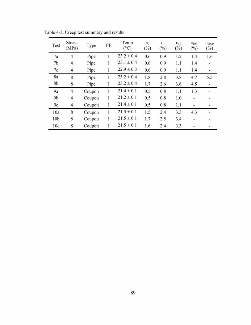
89

Table 4-3. Creep test summary and results

Test Stress (MPa) Type PE Temp

(°C) ε0

(%) ε1

(%) ε10 (%)

ε100 (%)

ε1000 (%)

7a 4 Pipe 1 23.2 ± 0.4 0.6 0.9 1.2 1.4 1.6 7b 4 Pipe 1 23.1 ± 0.4 0.6 0.9 1.1 1.4 - 7c 4 Pipe 1 22.9 ± 0.3 0.6 0.9 1.1 1.4 - 8a 8 Pipe 1 23.2 ± 0.4 1.8 2.8 3.8 4.7 5.5 8b 8 Pipe 1 23.2 ± 0.4 1.7 2.6 3.6 4.5 - 9a 4 Coupon 1 21.4 ± 0.1 0.5 0.8 1.1 1.3 - 9b 4 Coupon 1 21.2 ± 0.1 0.5 0.8 1.0 - - 9c 4 Coupon 1 21.4 ± 0.1 0.5 0.8 1.1 - -

10a 8 Coupon 1 21.5 ± 0.1 1.5 2.4 3.3 4.3 - 10b 8 Coupon 1 21.5 ± 0.1 1.7 2.5 3.4 - - 10c 8 Coupon 1 21.5 ± 0.1 1.6 2.4 3.3 - -

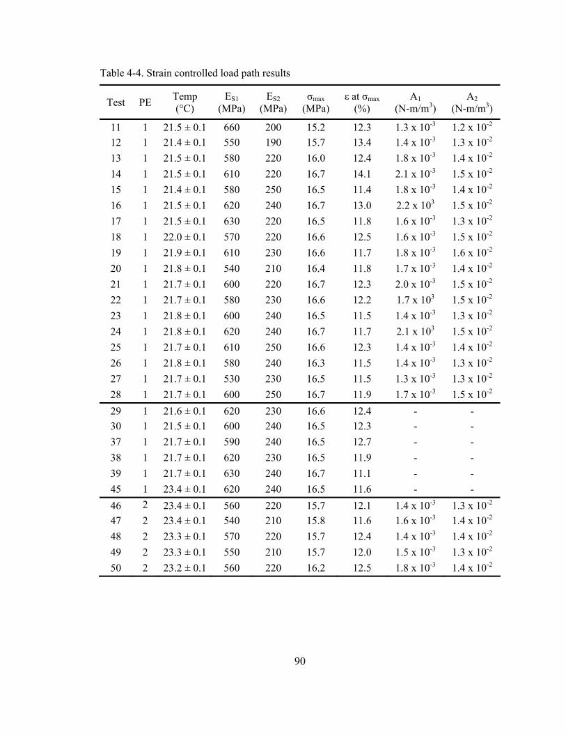
90

Table 4-4. Strain controlled load path results

Test PE Temp (°C)

ES1 (MPa)

ES2 (MPa)

σmax (MPa)

ε at σmax (%)

A1 (N-m/m3)

A2 (N-m/m3)

11 1 21.5 ± 0.1 660 200 15.2 12.3 1.3 x 10-3 1.2 x 10-2 12 1 21.4 ± 0.1 550 190 15.7 13.4 1.4 x 10-3 1.3 x 10-2 13 1 21.5 ± 0.1 580 220 16.0 12.4 1.8 x 10-3 1.4 x 10-2 14 1 21.5 ± 0.1 610 220 16.7 14.1 2.1 x 10-3 1.5 x 10-2 15 1 21.4 ± 0.1 580 250 16.5 11.4 1.8 x 10-3 1.4 x 10-2 16 1 21.5 ± 0.1 620 240 16.7 13.0 2.2 x 103 1.5 x 10-2 17 1 21.5 ± 0.1 630 220 16.5 11.8 1.6 x 10-3 1.3 x 10-2 18 1 22.0 ± 0.1 570 220 16.6 12.5 1.6 x 10-3 1.5 x 10-2 19 1 21.9 ± 0.1 610 230 16.6 11.7 1.8 x 10-3 1.6 x 10-2 20 1 21.8 ± 0.1 540 210 16.4 11.8 1.7 x 10-3 1.4 x 10-2 21 1 21.7 ± 0.1 600 220 16.7 12.3 2.0 x 10-3 1.5 x 10-2 22 1 21.7 ± 0.1 580 230 16.6 12.2 1.7 x 103 1.5 x 10-2 23 1 21.8 ± 0.1 600 240 16.5 11.5 1.4 x 10-3 1.3 x 10-2 24 1 21.8 ± 0.1 620 240 16.7 11.7 2.1 x 103 1.5 x 10-2 25 1 21.7 ± 0.1 610 250 16.6 12.3 1.4 x 10-3 1.4 x 10-2 26 1 21.8 ± 0.1 580 240 16.3 11.5 1.4 x 10-3 1.3 x 10-2 27 1 21.7 ± 0.1 530 230 16.5 11.5 1.3 x 10-3 1.3 x 10-2 28 1 21.7 ± 0.1 600 250 16.7 11.9 1.7 x 10-3 1.5 x 10-2 29 1 21.6 ± 0.1 620 230 16.6 12.4 - - 30 1 21.5 ± 0.1 600 240 16.5 12.3 - - 37 1 21.7 ± 0.1 590 240 16.5 12.7 - - 38 1 21.7 ± 0.1 620 230 16.5 11.9 - - 39 1 21.7 ± 0.1 630 240 16.7 11.1 - - 45 1 23.4 ± 0.1 620 240 16.5 11.6 - - 46 2 23.4 ± 0.1 560 220 15.7 12.1 1.4 x 10-3 1.3 x 10-2 47 2 23.4 ± 0.1 540 210 15.8 11.6 1.6 x 10-3 1.4 x 10-2 48 2 23.3 ± 0.1 570 220 15.7 12.4 1.4 x 10-3 1.4 x 10-2 49 2 23.3 ± 0.1 550 210 15.7 12.0 1.5 x 10-3 1.3 x 10-2 50 2 23.2 ± 0.1 560 220 16.2 12.5 1.8 x 10-3 1.4 x 10-2

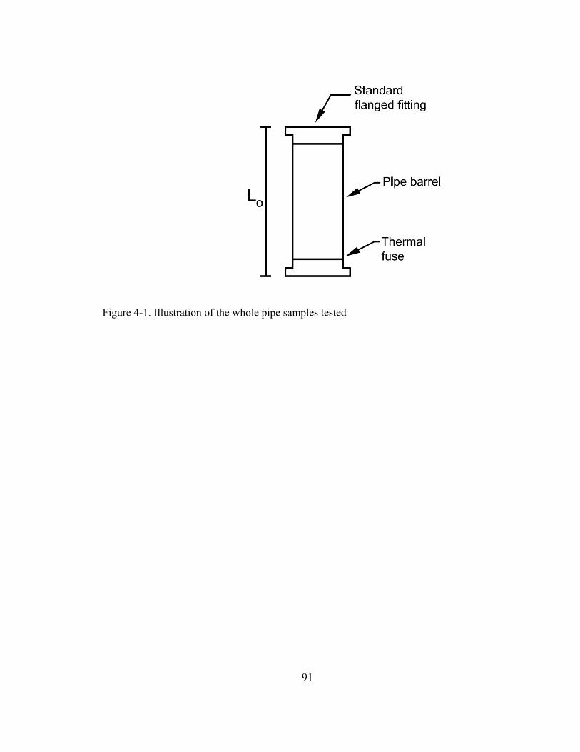
91

Figure 4-1. Illustration of the whole pipe samples tested

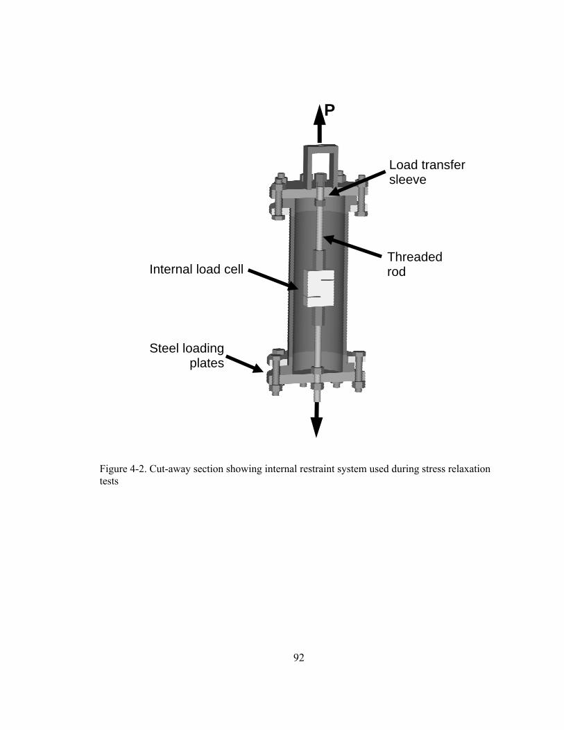
92

Figure 4-2. Cut-away section showing internal restraint system used during stress relaxation tests

Internal load cell

Load transfer sleeve

P

Threaded rod

Steel loading plates

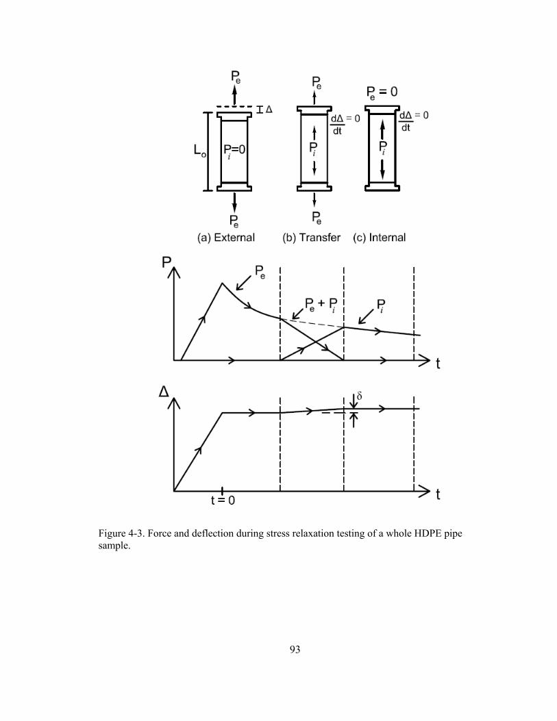
93

Figure 4-3. Force and deflection during stress relaxation testing of a whole HDPE pipe sample.

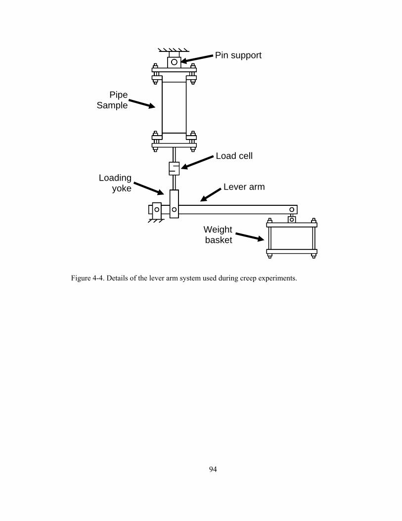
94

Figure 4-4. Details of the lever arm system used during creep experiments.

Load cell

Lever arm

Weight basket

Pipe Sample

Loading yoke

Pin support

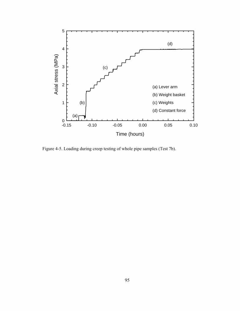
95

Time (hours)

-0.15 -0.10 -0.05 0.00 0.05 0.10

Axi

al s

tress

(MP

a)

0

1

2

3

4

5

(a)

(b)

(c)

(d)

(a) Lever arm

(b) Weight basket

(c) Weights

(d) Constant force

Figure 4-5. Loading during creep testing of whole pipe samples (Test 7b).

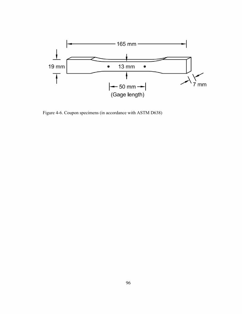
96

Figure 4-6. Coupon specimens (in accordance with ASTM D638)

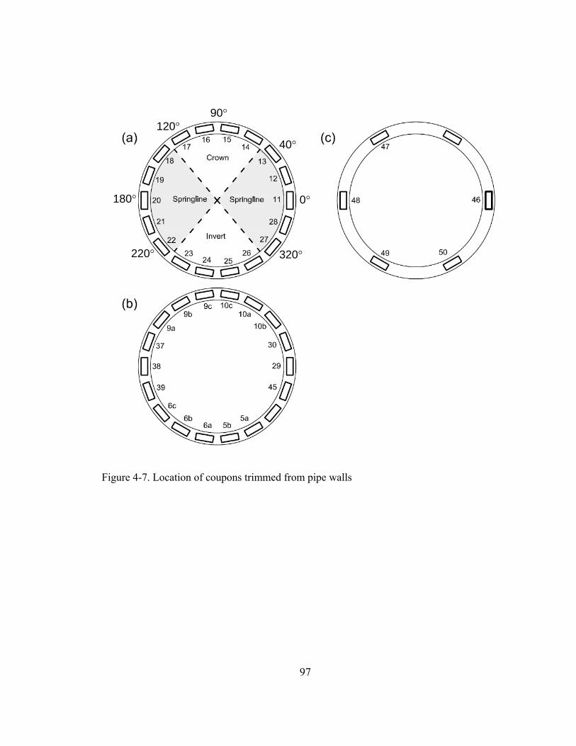
97

Figure 4-7. Location of coupons trimmed from pipe walls

0°

90°

180°

320° 220°

40° 120°

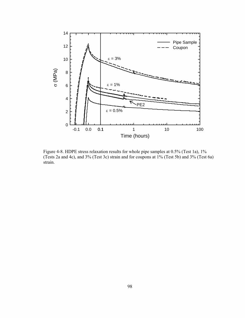
98

Time (hours)0.1 1 10 100

Pipe SampleCoupon

-0.1 0.0 0.1

σ (M

Pa)

0

2

4

6

8

10

12

14

ε = 3%

ε = 1%

ε = 0.5%PE2

Figure 4-8. HDPE stress relaxation results for whole pipe samples at 0.5% (Test 1a), 1% (Tests 2a and 4c), and 3% (Test 3c) strain and for coupons at 1% (Test 5b) and 3% (Test 6a) strain.

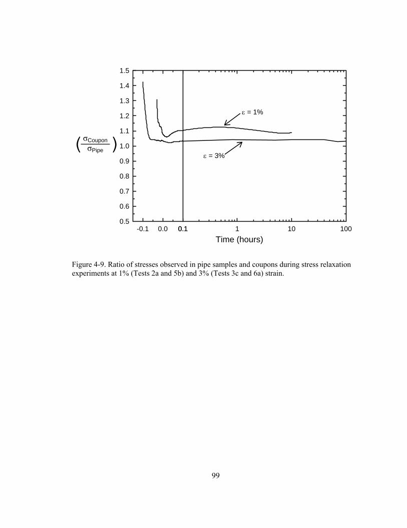
99

Time (hours)0.1 1 10 100-0.1 0.0 0.1

CouponPipe

0.5

0.6

0.7

0.8

0.9

1.0

1.1

1.2

1.3

1.4

1.5

ε = 3%

ε = 1%

( )

Figure 4-9. Ratio of stresses observed in pipe samples and coupons during stress relaxation experiments at 1% (Tests 2a and 5b) and 3% (Tests 3c and 6a) strain.

σCoupon σPipe ( )

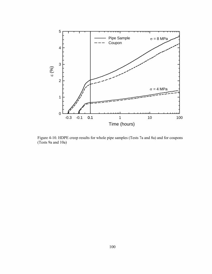
100

Time (hours)0.1 1 10 100

Pipe SampleCoupon

-0.3 -0.1 0.1

ε (%

)

0

1

2

3

4

5

σ = 8 MPa

σ = 4 MPa

Figure 4-10. HDPE creep results for whole pipe samples (Tests 7a and 8a) and for coupons (Tests 9a and 10a)

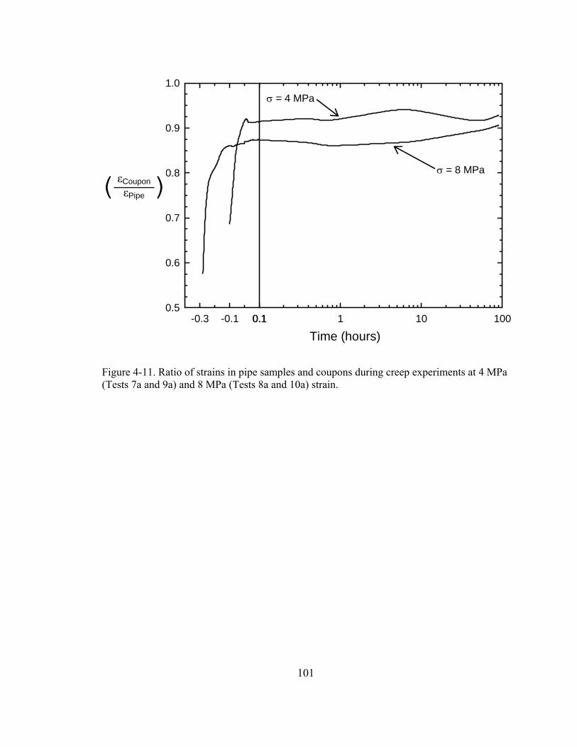
101

Time (hours)0.1 1 10 100

σ = 8 MPa

σ = 4 MPa

-0.3 -0.1 0.1

CouponPipe

0.5

0.6

0.7

0.8

0.9

1.0

( )

Figure 4-11. Ratio of strains in pipe samples and coupons during creep experiments at 4 MPa (Tests 7a and 9a) and 8 MPa (Tests 8a and 10a) strain.

εCoupon εPipe ( )

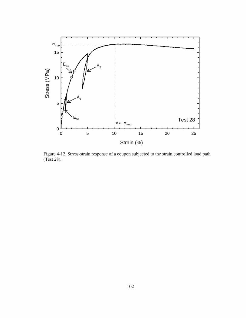
102

Strain (%)

0 5 10 15 20 25

Stre

ss (M

Pa)

0

5

10

15

Test 28

σmax

ε at σmax

ES1

ES2 A2

A1

Figure 4-12. Stress-strain response of a coupon subjected to the strain controlled load path (Test 28).

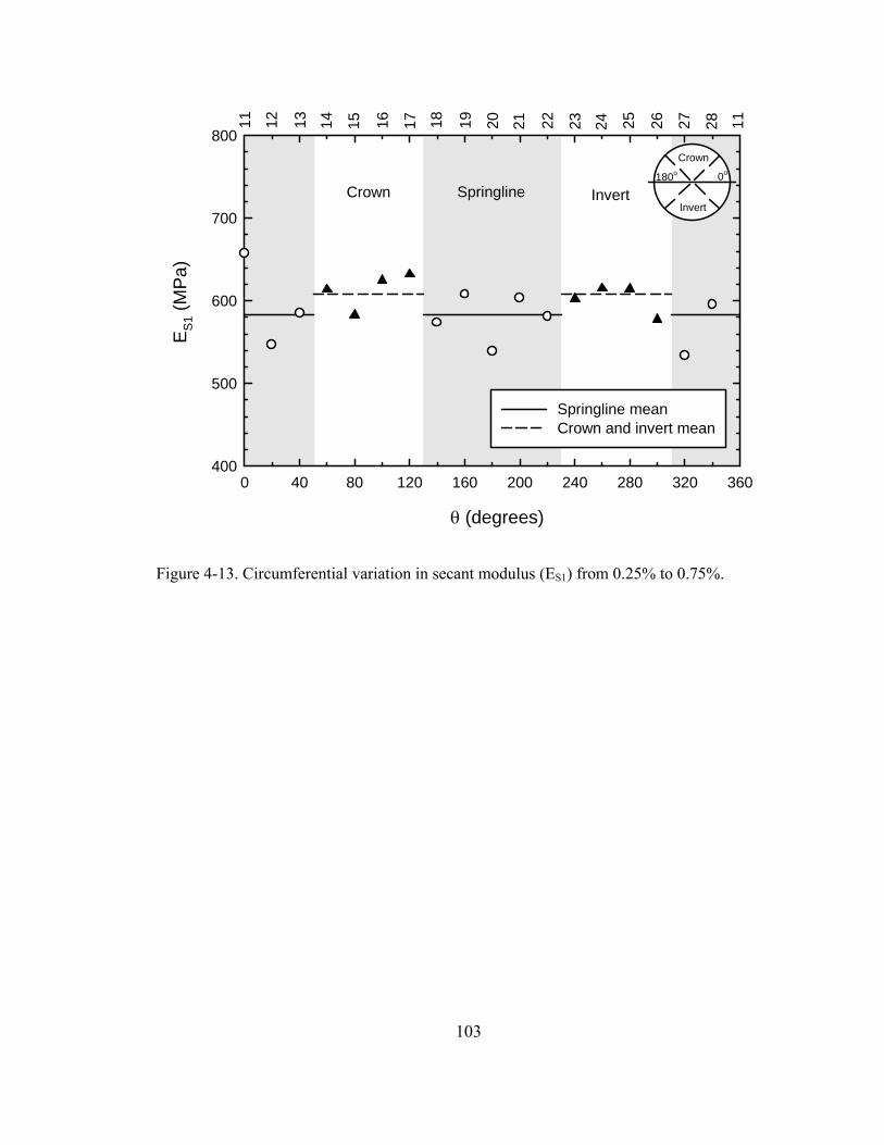
103

θ (degrees)

0 40 80 120 160 200 240 280 320 360

E S1 (

MP

a)

400

500

600

700

800

Springline meanCrown and invert mean

Crown InvertSpringline

28272625 1114131211 15 1716 18 2019 21 2322 24

0o

Crown

Invert

180o

Figure 4-13. Circumferential variation in secant modulus (ES1) from 0.25% to 0.75%.

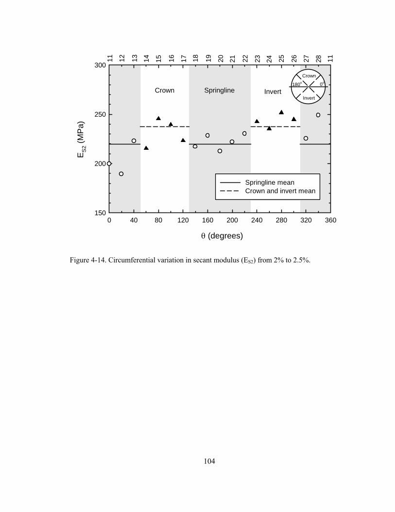
104

θ (degrees)

0 40 80 120 160 200 240 280 320 360

E S2 (

MP

a)

150

200

250

300

Crown InvertSpringline

28272625 1114131211 15 1716 18 2019 21 2322 24

Springline meanCrown and invert mean

0o

Crown

Invert

180o

Figure 4-14. Circumferential variation in secant modulus (ES2) from 2% to 2.5%.

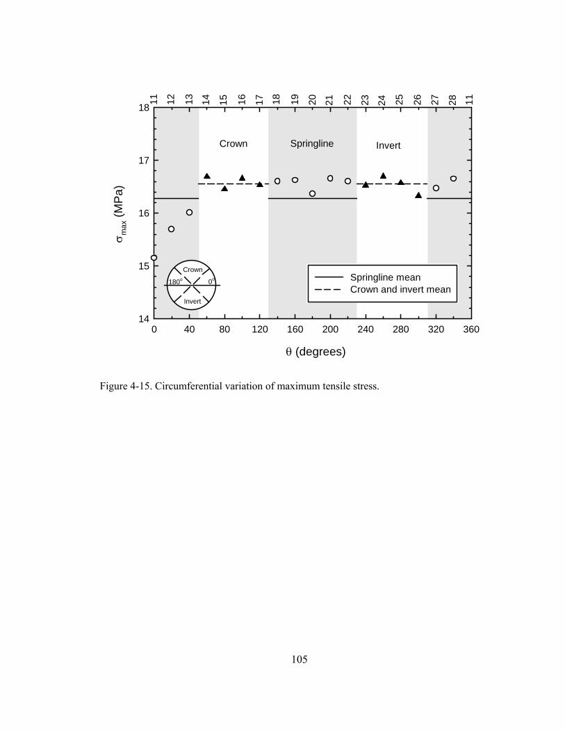
105

θ (degrees)

0 40 80 120 160 200 240 280 320 360

σ max

(MP

a)

14

15

16

17

18

Crown InvertSpringline

28272625 1114131211 15 1716 18 2019 21 2322 24

Springline meanCrown and invert mean

0o

Crown

Invert

180o

Figure 4-15. Circumferential variation of maximum tensile stress.

106

Chapter 5

Stress-strain measurements for HDPE pipe during and after

simulated installation by horizontal directional drilling

5.1 Introduction

Polymer pipelines can be installed using horizontal directional drilling, HDD, (e.g. see

ASTM F1962) as an alternative to traditional cut-and-cover trenching techniques. HDD

involves the creation of a borehole underground, Figure 5-1, with a drill bit that is controlled

from the ground surface. Once the borehole is in place, there are three essential stages for the

pipe during the HDD process: (1) a cyclic pulling force history is imposed on the new

polymer pipe (e.g., high density polyethylene, HDPE) as it is pulled into place, (2) the pipe is

unloaded to allow for the recovery of a portion of the axial extension incurred during

installation, and (3) the pipe is connected to a rigid structure such as a manhole, hydrant or

buried chamber.

During installation, the HDPE pipe is pulled through the ground in a series of steps as

each successive rod in the drill string is removed. Figure 5-2 provides the axial stress history

calculated from measurements of pulling force during installation of a nominal 220 mm

diameter DR11 (where DR is the ratio of the outside pipe diameter to minimum wall

thickness) HDPE pipe pulled 115 m through clay (Baumert, 2003). Figure 5-2 shows the

nature of the axial stresses experienced by the new HDPE pipe as it is installed. The peaks in

the stress history occur when the pipe is being pulled through the borehole, whereas the lower

values occur when the drill string is released to remove each successive drill rod. This cyclic

axial load history produces stresses and strains in the pipe which are not well understood.

107

The pipe can be designed to survive the short-term installation process by limiting the

maximum pulling force to some fraction of the short-term yield capacity of the pipe (ASTM

F1804; AWWA M55). However, once installed the long-term allowable performance limits

of the pipe are less than the short-term limits because HDPE is susceptible to slow crack

growth – a brittle failure mechanism occurring at tensile stresses well below short-term yield

(Mruk, 1990).

There is a paucity of data on what magnitude of tensile stresses can develop in pipes

installed by HDD and what factors may influence these tensile stresses. The objective of this

chapter is to quantify through physical experiments the axial stresses and strains that develop

in an HDPE pipe during and after a simulated HDD installation.

5.2 Experimental details

5.2.1 Pipe samples

Isolated HDPE pipe samples (i.e. not in contact with soil) were tested to investigate the

response of an HDPE pipe both during and after installation by HDD. When an HDPE pipe is

pulled-in-place during an HDD installation, the radial pressure acting on the outside of the

pipe (from the surrounding drilling fluid) is small compared to the tensile axial stress

imposed to install the pipe. Therefore, the stresses acting on the pipe are essentially one-

dimensional; suggesting testing isolated pipe samples to investigate the response of an HDPE

pipe is a reasonable approximation to field conditions. The entire barrel of the pipe was tested

rather than using coupons trimmed from the pipe as discussed in Chapter 4. This approach

eliminated the potential for sample disturbance (e.g., release of residual stresses) when

specimens are cut from a pipe wall.

108

The HDPE pipes tested were obtained from one manufacturer, but from two different

manufacturing plants. The two types of pipes are denoted as PE1 and PE2. Six pipe samples

of PE1 and twenty pipe samples of PE2 were tested. The outside diameter, wall thickness,

and length of the pipe samples are given in Table 5-1. On average, the outside diameter and

length of PE2 was only slightly smaller (less than 0.5%) than PE1, whereas the wall

thickness of PE1 was greater (by approximately 4%) than PE2.

Both pipe materials are designated PE 3408, which is an augmented grade

designation after ASTM D3350 by the Plastic Pipe Institute (PPI, 2006). To quantify the

difference between PE1 and PE2, polymer crystallinity and density were measured. These

results are given in Table 5-2. Polymer stiffness and tensile strength at yield increase when

the density and crystallinity are increased (PPI, 2006). The differences in density and

crystallinity between PE1 and PE2 are statistically significant at a 95% confidence level, with

PE1 having slightly larger values than PE2.

5.2.2 Simulation sequence

The applied force (P) and resulting deflection (Δ) with time (t) of a pipe sample during the

three stages simulated in the laboratory (installation, recovery, and restraint) are illustrated in

Figure 5-3. First, a cyclic axial force history is applied to the pipe sample, where N is the

number of load-unload cycles. During each cycle, Pp is the axial force applied to simulate the

force required to pull the pipe through the borehole and Pr is the axial force applied to

simulate the residual force when a drill rod is removed. Forces Pp and Pr are imposed over

time intervals tP and tr, respectively. After i number of cycles, the corresponding axial

deflection is Δi which reaches a maximum (Δmax) when i = N.

109

Once installed (taken here as time t = 0), the pipe sample is unloaded (P = 0) and a

portion of the displacement accumulated is recovered, as shown in Figure 5-3. After 120

seconds the deflection (relative to the initial length of the pipe) is defined as Δ120 s and ΔR

after the recovery period (tR).

For t > tR, the pipe length is then fixed (i.e. Δ=ΔR), simulating the pipe response as it

is attached to a rigid structure such as a manhole, hydrant, or buried chamber. The resistance

imposed to prevent any additional recovery leads to tensile axial forces redeveloping in the

pipe, reaching P100 hr after 100 hours, see Figure 5-3. The value of P100 hr does not increase

indefinitely over the service life of the HDPE pipe. Typically a maximum would be expected

to be reached and then these tensile forces would decrease due to stress relaxation.

5.2.3 Test method and instrumentation

The cyclic stress history was applied using a universal test machine (Instron 1350) through

steel flanges bolted onto standard HDPE flanged fittings which were thermally fused to the

ends of the pipe samples (identical to the pipe samples tested in Chapter 4). A load cell

associated with the universal test machine, having an accuracy of ± 75 N, was used to ensure

the correct force history was applied. To restrain the pipe and measure the redevelopment of

axial forces, a rigid internal mechanism was used in conjunction with a load cell accurate to ±

10 N. Displacements were measured using two linear potentiometers mounted on the outside

of the pipe sample having an accuracy of ± 0.01 mm. The tests were conducted at an average

temperature of 23°C with the specific details for each test given in Table 5-3. Application of

these results to lower temperatures (e.g. possible ground temperatures at depth) would

overestimate the magnitude of tensile strains that might develop during installation and the

rate that these strains are recovered after installation.

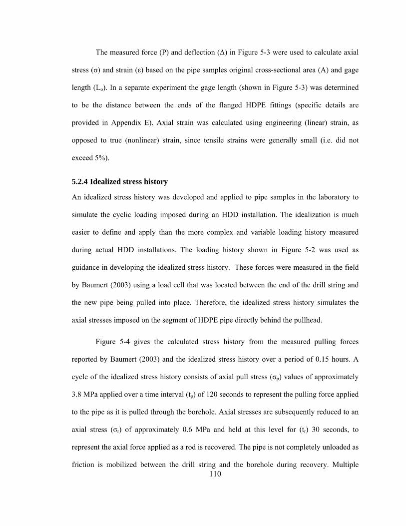
110

The measured force (P) and deflection (Δ) in Figure 5-3 were used to calculate axial

stress (σ) and strain (ε) based on the pipe samples original cross-sectional area (A) and gage

length (Lo). In a separate experiment the gage length (shown in Figure 5-3) was determined

to be the distance between the ends of the flanged HDPE fittings (specific details are

provided in Appendix E). Axial strain was calculated using engineering (linear) strain, as

opposed to true (nonlinear) strain, since tensile strains were generally small (i.e. did not

exceed 5%).

5.2.4 Idealized stress history

An idealized stress history was developed and applied to pipe samples in the laboratory to

simulate the cyclic loading imposed during an HDD installation. The idealization is much

easier to define and apply than the more complex and variable loading history measured

during actual HDD installations. The loading history shown in Figure 5-2 was used as

guidance in developing the idealized stress history. These forces were measured in the field

by Baumert (2003) using a load cell that was located between the end of the drill string and

the new pipe being pulled into place. Therefore, the idealized stress history simulates the

axial stresses imposed on the segment of HDPE pipe directly behind the pullhead.

Figure 5-4 gives the calculated stress history from the measured pulling forces

reported by Baumert (2003) and the idealized stress history over a period of 0.15 hours. A

cycle of the idealized stress history consists of axial pull stress (σp) values of approximately

3.8 MPa applied over a time interval (tp) of 120 seconds to represent the pulling force applied

to the pipe as it is pulled through the borehole. Axial stresses are subsequently reduced to an

axial stress (σr) of approximately 0.6 MPa and held at this level for (tr) 30 seconds, to

represent the axial force applied as a rod is recovered. The pipe is not completely unloaded as

friction is mobilized between the drill string and the borehole during recovery. Multiple

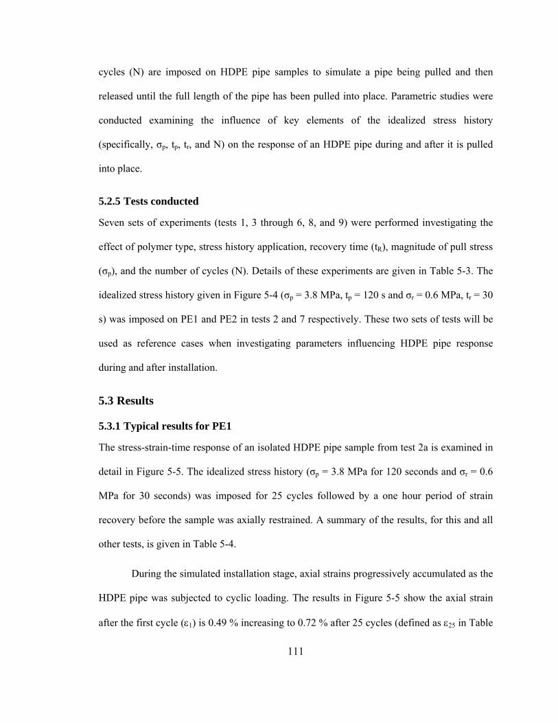
111

cycles (N) are imposed on HDPE pipe samples to simulate a pipe being pulled and then

released until the full length of the pipe has been pulled into place. Parametric studies were

conducted examining the influence of key elements of the idealized stress history

(specifically, σp, tp, tr, and N) on the response of an HDPE pipe during and after it is pulled

into place.

5.2.5 Tests conducted

Seven sets of experiments (tests 1, 3 through 6, 8, and 9) were performed investigating the

effect of polymer type, stress history application, recovery time (tR), magnitude of pull stress

(σp), and the number of cycles (N). Details of these experiments are given in Table 5-3. The

idealized stress history given in Figure 5-4 (σp = 3.8 MPa, tp = 120 s and σr = 0.6 MPa, tr = 30

s) was imposed on PE1 and PE2 in tests 2 and 7 respectively. These two sets of tests will be

used as reference cases when investigating parameters influencing HDPE pipe response

during and after installation.

5.3 Results

5.3.1 Typical results for PE1

The stress-strain-time response of an isolated HDPE pipe sample from test 2a is examined in

detail in Figure 5-5. The idealized stress history (σp = 3.8 MPa for 120 seconds and σr = 0.6

MPa for 30 seconds) was imposed for 25 cycles followed by a one hour period of strain

recovery before the sample was axially restrained. A summary of the results, for this and all

other tests, is given in Table 5-4.

During the simulated installation stage, axial strains progressively accumulated as the

HDPE pipe was subjected to cyclic loading. The results in Figure 5-5 show the axial strain

after the first cycle (ε1) is 0.49 % increasing to 0.72 % after 25 cycles (defined as ε25 in Table

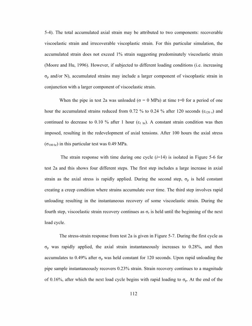
112

5-4). The total accumulated axial strain may be attributed to two components: recoverable

viscoelastic strain and irrecoverable viscoplastic strain. For this particular simulation, the

accumulated strain does not exceed 1% strain suggesting predominately viscoelastic strain

(Moore and Hu, 1996). However, if subjected to different loading conditions (i.e. increasing

σp and/or N), accumulated strains may include a larger component of viscoplastic strain in

conjunction with a larger component of viscoelastic strain.

When the pipe in test 2a was unloaded (σ = 0 MPa) at time t=0 for a period of one

hour the accumulated strains reduced from 0.72 % to 0.24 % after 120 seconds (ε120 s) and

continued to decrease to 0.10 % after 1 hour (ε1 hr). A constant strain condition was then

imposed, resulting in the redevelopment of axial tensions. After 100 hours the axial stress

(σ100 hr) in this particular test was 0.49 MPa.

The strain response with time during one cycle (i=14) is isolated in Figure 5-6 for

test 2a and this shows four different steps. The first step includes a large increase in axial

strain as the axial stress is rapidly applied. During the second step, σp is held constant

creating a creep condition where strains accumulate over time. The third step involves rapid

unloading resulting in the instantaneous recovery of some viscoelastic strain. During the

fourth step, viscoelastic strain recovery continues as σr is held until the beginning of the next

load cycle.

The stress-strain response from test 2a is given in Figure 5-7. During the first cycle as

σp was rapidly applied, the axial strain instantaneously increases to 0.28%, and then

accumulates to 0.49% after σp was held constant for 120 seconds. Upon rapid unloading the

pipe sample instantaneously recovers 0.23% strain. Strain recovery continues to a magnitude

of 0.16%, after which the next load cycle begins with rapid loading to σp. At the end of the

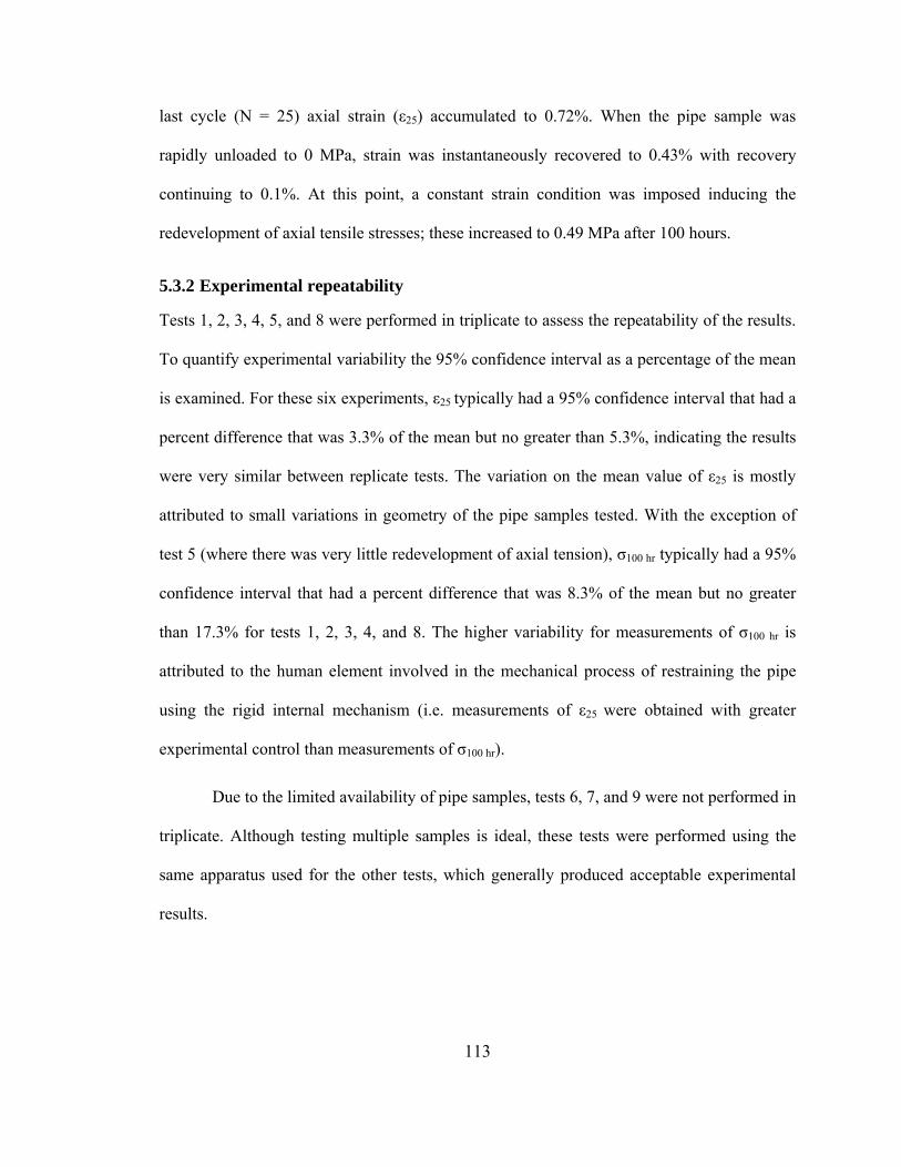
113

last cycle (N = 25) axial strain (ε25) accumulated to 0.72%. When the pipe sample was

rapidly unloaded to 0 MPa, strain was instantaneously recovered to 0.43% with recovery

continuing to 0.1%. At this point, a constant strain condition was imposed inducing the

redevelopment of axial tensile stresses; these increased to 0.49 MPa after 100 hours.

5.3.2 Experimental repeatability

Tests 1, 2, 3, 4, 5, and 8 were performed in triplicate to assess the repeatability of the results.

To quantify experimental variability the 95% confidence interval as a percentage of the mean

is examined. For these six experiments, ε25 typically had a 95% confidence interval that had a

percent difference that was 3.3% of the mean but no greater than 5.3%, indicating the results

were very similar between replicate tests. The variation on the mean value of ε25 is mostly

attributed to small variations in geometry of the pipe samples tested. With the exception of

test 5 (where there was very little redevelopment of axial tension), σ100 hr typically had a 95%

confidence interval that had a percent difference that was 8.3% of the mean but no greater

than 17.3% for tests 1, 2, 3, 4, and 8. The higher variability for measurements of σ100 hr is

attributed to the human element involved in the mechanical process of restraining the pipe

using the rigid internal mechanism (i.e. measurements of ε25 were obtained with greater

experimental control than measurements of σ100 hr).

Due to the limited availability of pipe samples, tests 6, 7, and 9 were not performed in

triplicate. Although testing multiple samples is ideal, these tests were performed using the

same apparatus used for the other tests, which generally produced acceptable experimental

results.

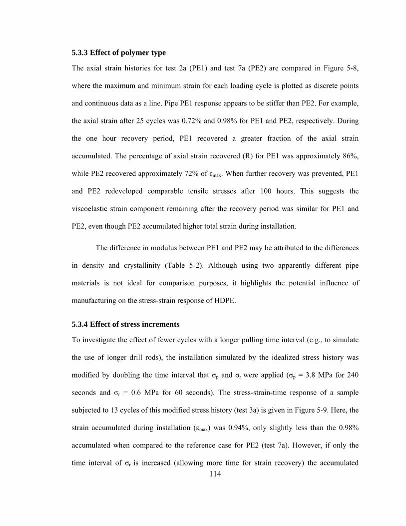
114

5.3.3 Effect of polymer type

The axial strain histories for test 2a (PE1) and test 7a (PE2) are compared in Figure 5-8,

where the maximum and minimum strain for each loading cycle is plotted as discrete points

and continuous data as a line. Pipe PE1 response appears to be stiffer than PE2. For example,

the axial strain after 25 cycles was 0.72% and 0.98% for PE1 and PE2, respectively. During

the one hour recovery period, PE1 recovered a greater fraction of the axial strain

accumulated. The percentage of axial strain recovered (R) for PE1 was approximately 86%,

while PE2 recovered approximately 72% of εmax. When further recovery was prevented, PE1

and PE2 redeveloped comparable tensile stresses after 100 hours. This suggests the

viscoelastic strain component remaining after the recovery period was similar for PE1 and

PE2, even though PE2 accumulated higher total strain during installation.

The difference in modulus between PE1 and PE2 may be attributed to the differences

in density and crystallinity (Table 5-2). Although using two apparently different pipe

materials is not ideal for comparison purposes, it highlights the potential influence of

manufacturing on the stress-strain response of HDPE.

5.3.4 Effect of stress increments

To investigate the effect of fewer cycles with a longer pulling time interval (e.g., to simulate

the use of longer drill rods), the installation simulated by the idealized stress history was

modified by doubling the time interval that σp and σr were applied (σp = 3.8 MPa for 240

seconds and σr = 0.6 MPa for 60 seconds). The stress-strain-time response of a sample

subjected to 13 cycles of this modified stress history (test 3a) is given in Figure 5-9. Here, the

strain accumulated during installation (εmax) was 0.94%, only slightly less than the 0.98%

accumulated when compared to the reference case for PE2 (test 7a). However, if only the

time interval of σr is increased (allowing more time for strain recovery) the accumulated

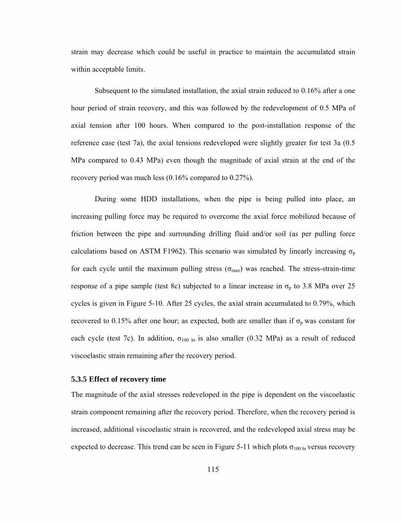
115

strain may decrease which could be useful in practice to maintain the accumulated strain

within acceptable limits.

Subsequent to the simulated installation, the axial strain reduced to 0.16% after a one

hour period of strain recovery, and this was followed by the redevelopment of 0.5 MPa of

axial tension after 100 hours. When compared to the post-installation response of the

reference case (test 7a), the axial tensions redeveloped were slightly greater for test 3a (0.5

MPa compared to 0.43 MPa) even though the magnitude of axial strain at the end of the

recovery period was much less (0.16% compared to 0.27%).

During some HDD installations, when the pipe is being pulled into place, an

increasing pulling force may be required to overcome the axial force mobilized because of

friction between the pipe and surrounding drilling fluid and/or soil (as per pulling force

calculations based on ASTM F1962). This scenario was simulated by linearly increasing σp

for each cycle until the maximum pulling stress (σmax) was reached. The stress-strain-time

response of a pipe sample (test 8c) subjected to a linear increase in σp to 3.8 MPa over 25

cycles is given in Figure 5-10. After 25 cycles, the axial strain accumulated to 0.79%, which

recovered to 0.15% after one hour; as expected, both are smaller than if σp was constant for

each cycle (test 7c). In addition, σ100 hr is also smaller (0.32 MPa) as a result of reduced

viscoelastic strain remaining after the recovery period.

5.3.5 Effect of recovery time

The magnitude of the axial stresses redeveloped in the pipe is dependent on the viscoelastic

strain component remaining after the recovery period. Therefore, when the recovery period is

increased, additional viscoelastic strain is recovered, and the redeveloped axial stress may be

expected to decrease. This trend can be seen in Figure 5-11 which plots σ100 hr versus recovery

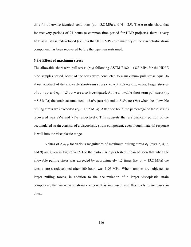
116

time for otherwise identical conditions (σp = 3.8 MPa and N = 25). These results show that

for recovery periods of 24 hours (a common time period for HDD projects), there is very

little axial stress redeveloped (i.e. less than 0.10 MPa) as a majority of the viscoelastic strain

component has been recovered before the pipe was restrained.

5.3.6 Effect of maximum stress

The allowable short-term pull stress (σall) following ASTM F1804 is 8.3 MPa for the HDPE

pipe samples tested. Most of the tests were conducted to a maximum pull stress equal to

about one-half of the allowable short-term stress (i.e. σp ≈ 0.5 σall); however, larger stresses

of σp ≈ σall and σp ≈ 1.5 σall were also investigated. At the allowable short-term pull stress (σp

= 8.3 MPa) the strain accumulated to 3.0% (test 4a) and to 8.3% (test 9a) when the allowable

pulling stress was exceeded (σp = 13.2 MPa). After one hour, the percentage of these strains

recovered was 78% and 71% respectively. This suggests that a significant portion of the

accumulated strain consists of a viscoelastic strain component, even though material response

is well into the viscoplastic range.

Values of σ100 hr for various magnitudes of maximum pulling stress σp (tests 2, 4, 7,

and 9) are given in Figure 5-12. For the particular pipes tested, it can be seen that when the

allowable pulling stress was exceeded by approximately 1.5 times (i.e. σp = 13.2 MPa) the

tensile stress redeveloped after 100 hours was 1.99 MPa. When samples are subjected to

larger pulling forces, in addition to the accumulation of a larger viscoplastic strain

component, the viscoelastic strain component is increased, and this leads to increases in

σ100hr.

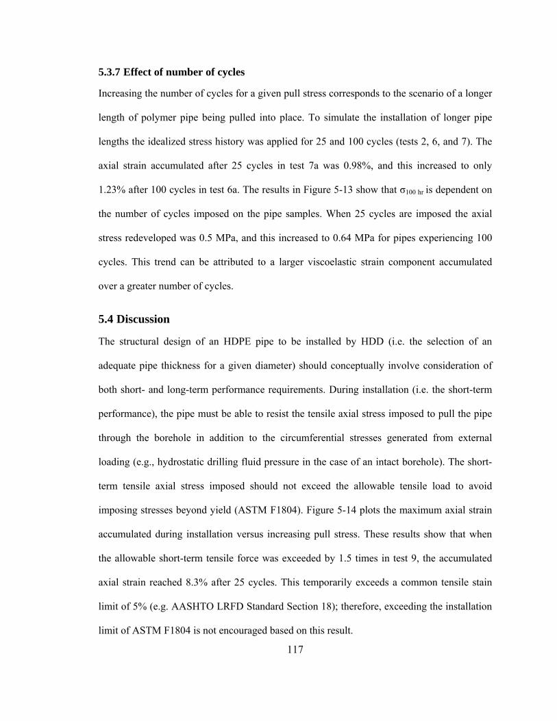
117

5.3.7 Effect of number of cycles

Increasing the number of cycles for a given pull stress corresponds to the scenario of a longer

length of polymer pipe being pulled into place. To simulate the installation of longer pipe

lengths the idealized stress history was applied for 25 and 100 cycles (tests 2, 6, and 7). The

axial strain accumulated after 25 cycles in test 7a was 0.98%, and this increased to only

1.23% after 100 cycles in test 6a. The results in Figure 5-13 show that σ100 hr is dependent on

the number of cycles imposed on the pipe samples. When 25 cycles are imposed the axial

stress redeveloped was 0.5 MPa, and this increased to 0.64 MPa for pipes experiencing 100

cycles. This trend can be attributed to a larger viscoelastic strain component accumulated

over a greater number of cycles.

5.4 Discussion

The structural design of an HDPE pipe to be installed by HDD (i.e. the selection of an

adequate pipe thickness for a given diameter) should conceptually involve consideration of

both short- and long-term performance requirements. During installation (i.e. the short-term

performance), the pipe must be able to resist the tensile axial stress imposed to pull the pipe

through the borehole in addition to the circumferential stresses generated from external

loading (e.g., hydrostatic drilling fluid pressure in the case of an intact borehole). The short-

term tensile axial stress imposed should not exceed the allowable tensile load to avoid

imposing stresses beyond yield (ASTM F1804). Figure 5-14 plots the maximum axial strain

accumulated during installation versus increasing pull stress. These results show that when

the allowable short-term tensile force was exceeded by 1.5 times in test 9, the accumulated

axial strain reached 8.3% after 25 cycles. This temporarily exceeds a common tensile stain

limit of 5% (e.g. AASHTO LRFD Standard Section 18); therefore, exceeding the installation

limit of ASTM F1804 is not encouraged based on this result.

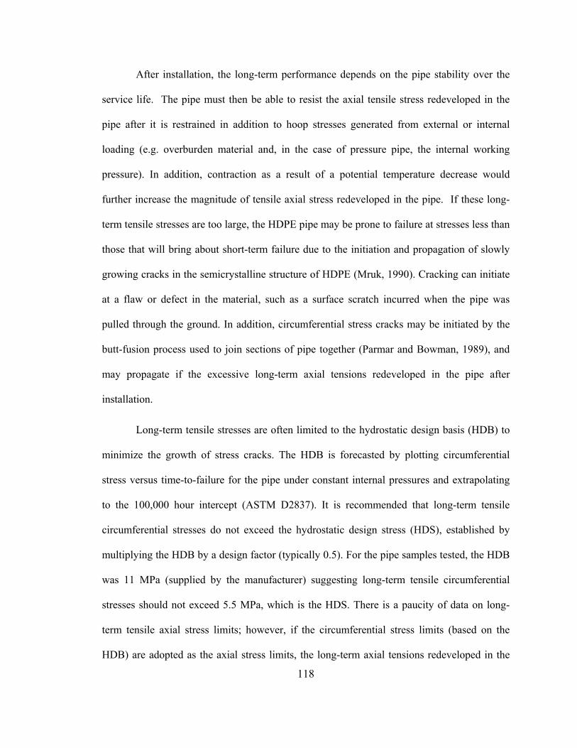
118

After installation, the long-term performance depends on the pipe stability over the

service life. The pipe must then be able to resist the axial tensile stress redeveloped in the

pipe after it is restrained in addition to hoop stresses generated from external or internal

loading (e.g. overburden material and, in the case of pressure pipe, the internal working

pressure). In addition, contraction as a result of a potential temperature decrease would

further increase the magnitude of tensile axial stress redeveloped in the pipe. If these long-

term tensile stresses are too large, the HDPE pipe may be prone to failure at stresses less than

those that will bring about short-term failure due to the initiation and propagation of slowly

growing cracks in the semicrystalline structure of HDPE (Mruk, 1990). Cracking can initiate

at a flaw or defect in the material, such as a surface scratch incurred when the pipe was

pulled through the ground. In addition, circumferential stress cracks may be initiated by the

butt-fusion process used to join sections of pipe together (Parmar and Bowman, 1989), and

may propagate if the excessive long-term axial tensions redeveloped in the pipe after

installation.

Long-term tensile stresses are often limited to the hydrostatic design basis (HDB) to

minimize the growth of stress cracks. The HDB is forecasted by plotting circumferential

stress versus time-to-failure for the pipe under constant internal pressures and extrapolating

to the 100,000 hour intercept (ASTM D2837). It is recommended that long-term tensile

circumferential stresses do not exceed the hydrostatic design stress (HDS), established by

multiplying the HDB by a design factor (typically 0.5). For the pipe samples tested, the HDB

was 11 MPa (supplied by the manufacturer) suggesting long-term tensile circumferential

stresses should not exceed 5.5 MPa, which is the HDS. There is a paucity of data on long-

term tensile axial stress limits; however, if the circumferential stress limits (based on the

HDB) are adopted as the axial stress limits, the long-term axial tensions redeveloped in the

119

particular pipes tested should not exceed 5.5 MPa (HDS) to ensure adequate long-term

performance.

For the conditions simulated in the laboratory, the tensile axial stress redeveloped in

the pipe did not exceed the HDS. Even when short-term performance limits were exceeded

during installation and allowed to recover for at least 1 hour, the tensile stresses that develop

after 100 hours were below the HDS. For the particular pipes tested, this suggests that

exceeding the short-term limits during installation by a factor of 1.5 did not jeopardize the

service life of the pipes. However, if the redeveloped stresses were deemed to be excessive,

the recovery period (tR) can be extended to minimize the magnitude of the redeveloped

stresses.

5.5 Conclusions

Experimental results from a laboratory investigation of HDPE pipe response during and after

installation by horizontal directional drilling were presented. Tensile axial stresses and strains

in the pipe were quantified during cyclic loading, strain recovery, and stress redevelopment

after the pipe is restrained leading to the following conclusions:

(i) During a typical HDD installation the HDPE pipe being installed will experience

a complex stress and strain history including periods of rapid loading, creep, rapid

unloading, and strain recovery as the pipe is pulled then released to remove each

subsequent drill rod. During installation, axial strains progressively accumulate as

the pipe is installed. This is followed by a period of axial strain recovery.

Subsequently, the pipe is axially restrained which leads to a build-up of axial

tensions.

120

(ii) It was shown that the maximum strain of the HDPE pipe samples depends on the

magnitude of the pulling force, length of pipe installed, and drilling rod length.

Longer lengths of pipe installed and increased pulling forces led to higher

maximum strains. When the allowable pulling stress was exceeded by a factor of

1.5 the axial strain accumulated was 8.3%, surpassing the generally accepted

strain limit of 5% for HDPE.

(iii) When subjected to identical pulling force histories, HDPE pipe samples

manufactured on different production lines responded differently highlighting the

influence of crystallinity and density on the stress-strain response of HDPE.

(iv) The redevelopment of tensile axial stress is caused by the resistance required to

prevent further recovery of the viscoelastic strain component. For the particular

pipes tested, very little axial stresses were redeveloped in the pipe (i.e. less than

0.1 MPa) after a recovery period of 24 hours that is typical of what occurs during

field operations.

(v) Tensile axial stress levels that redeveloped in the pipes did not exceed possible

long-term performance limits for HDPE. Even when the short-term performance

limits were exceeded, the long-term axial tensions that redeveloped did not

exceed the hydrostatic design stress of 5.5 MPa applicable to the particular pipes

that were tested.

For the specific conditions examined, none of the measured data suggests that the

HDPE pipes subjected to the simulated installation sequence would experience long-term

tensile stresses that would lead to stress conditions conducive to slow crack growth. On the

contrary, the available data suggests that limiting the installation force to values stipulated by

121

ASTM F1804 and allowing a minimum of 24 hrs of recovery time is sufficient to ensure

adequate long-term pipe performance from installation induced tensile axial stresses.

5.6 References

AWWA M55. PE Pipe – Design and Installation (M55). American Water Works Association,

Denver, COL.

AASHTO, Load and Resistance Factor Design Bridge Design Specifications, 4th edition,

Washington, DC, American Association of State Transportation Officials, 2007.

ASTM E 794-95. Standard Test Method for Melting and Crystallization Temperatures by

Thermal Analysis. ASTM International, West Conshohocken, PA.

ASTM D 1505-03. Standard Test Method for Density of Plastics by the Density-Gradient

Technique. ASTM International, West Conshohocken, PA.

ASTM F 1804-08. Standard Practice for Determining Allowable Tensile Load for

Polyethylene (PE) Gas Pipe During Pull-In Installation. ASTM International, West

Conshohocken, PA.

ASTM F 1962-05 Standard Guide for Use of Maxi-Horizontal Directional Drilling for

Placement of Polyethylene Pipe or Conduit Under Obstacles, Including River Crossings.

ASTM International, West Conshohocken, PA.

ASTM D 2837-04. Standard Test Method for Obtaining Hydrostatic Design Basis for

Thermoplastic Pipe Materials or Pressure Design Basis for Thermoplastic Pipe Products.

ASTM International, West Conshohocken, PA.

ASTM D 3350-08. Standard Specification for Polyethylene Plastics Pipe and Fittings

Materials. ASTM International, West Conshohocken, PA.

Baumert, M.E. 2003. Experimental investigation of pulling loads and mud pressures during

horizontal directional drilling installations. PhD Thesis, The University of Western

Ontario, London, Ontario.

122

Moore, I D and Hu, F, 1996, Linear viscoelastic modeling of profiled high density

polyethylene pipe, Canadian Journal of Civil Engineering, 23: 395-407.

Moore, I.D. and Zhang, C. 1997. Nonlinear mechanical response of high density

polyethylene. Part I: Experimental investigation and model evaluation. Polymer

Engineering and Science, Vol. 37, No.2: 404-413

Mruk, S.A. 1990. The durability of polyethylene piping. Buried Plastic Pipe Technology.

ASTM STP 1093, G.S. Buczala and M.J. Cassady (Eds.) ASCE, pp 21-39

Parmar, R., and Bowman, J. 1989. Crack initiation and propagation paths for brittle failures

in aligned and misaligned pipe butt fusion joints. Polymer Science and Engineering,

29(19):1396-1405.

PPI Handbook of Polyethylene Pipe, 1st ed., 2006. pp 47-156. Plastic Pipe Institute, Irving,

TX.

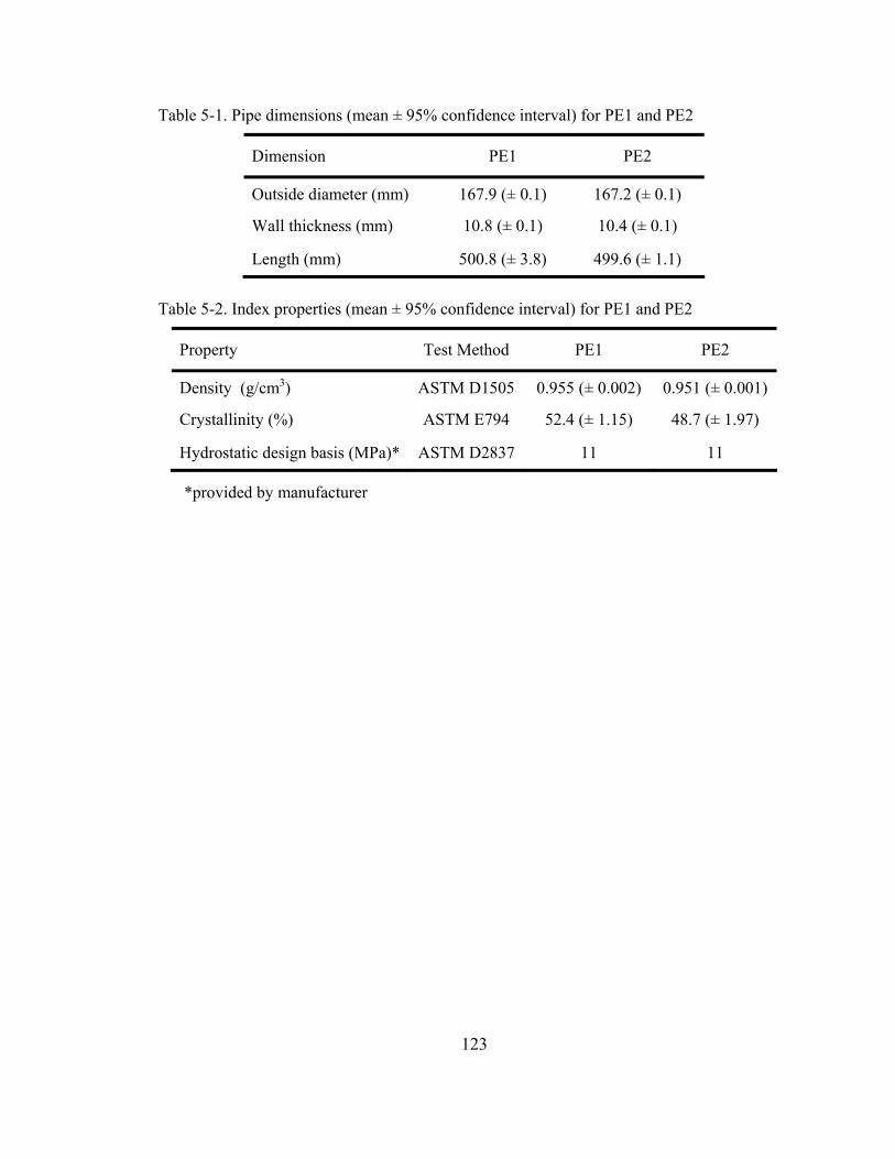
123

Table 5-1. Pipe dimensions (mean ± 95% confidence interval) for PE1 and PE2

Dimension PE1 PE2

Outside diameter (mm) 167.9 (± 0.1) 167.2 (± 0.1)

Wall thickness (mm) 10.8 (± 0.1) 10.4 (± 0.1)

Length (mm) 500.8 (± 3.8) 499.6 (± 1.1)

Table 5-2. Index properties (mean ± 95% confidence interval) for PE1 and PE2

Property Test Method PE1 PE2

Density (g/cm3) ASTM D1505 0.955 (± 0.002) 0.951 (± 0.001)

Crystallinity (%) ASTM E794 52.4 (± 1.15) 48.7 (± 1.97)

Hydrostatic design basis (MPa)* ASTM D2837 11 11

*provided by manufacturer

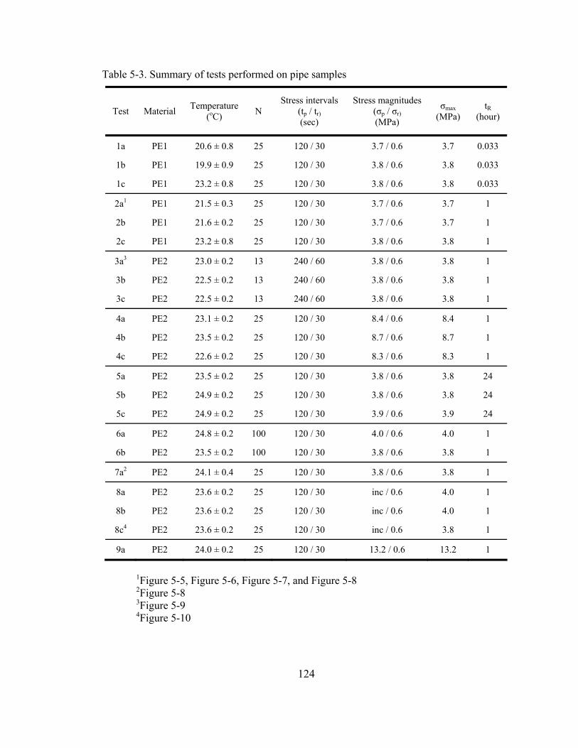
124

Table 5-3. Summary of tests performed on pipe samples

Test Material Temperature (oC) N

Stress intervals(tp / tr) (sec)

Stress magnitudes (σp / σr) (MPa)

σmax (MPa)

tR (hour)

1a PE1 20.6 ± 0.8 25 120 / 30 3.7 / 0.6 3.7 0.033

1b PE1 19.9 ± 0.9 25 120 / 30 3.8 / 0.6 3.8 0.033

1c PE1 23.2 ± 0.8 25 120 / 30 3.8 / 0.6 3.8 0.033

2a1 PE1 21.5 ± 0.3 25 120 / 30 3.7 / 0.6 3.7 1

2b PE1 21.6 ± 0.2 25 120 / 30 3.7 / 0.6 3.7 1

2c PE1 23.2 ± 0.8 25 120 / 30 3.8 / 0.6 3.8 1

3a3 PE2 23.0 ± 0.2 13 240 / 60 3.8 / 0.6 3.8 1

3b PE2 22.5 ± 0.2 13 240 / 60 3.8 / 0.6 3.8 1

3c PE2 22.5 ± 0.2 13 240 / 60 3.8 / 0.6 3.8 1

4a PE2 23.1 ± 0.2 25 120 / 30 8.4 / 0.6 8.4 1

4b PE2 23.5 ± 0.2 25 120 / 30 8.7 / 0.6 8.7 1

4c PE2 22.6 ± 0.2 25 120 / 30 8.3 / 0.6 8.3 1

5a PE2 23.5 ± 0.2 25 120 / 30 3.8 / 0.6 3.8 24

5b PE2 24.9 ± 0.2 25 120 / 30 3.8 / 0.6 3.8 24

5c PE2 24.9 ± 0.2 25 120 / 30 3.9 / 0.6 3.9 24

6a PE2 24.8 ± 0.2 100 120 / 30 4.0 / 0.6 4.0 1

6b PE2 23.5 ± 0.2 100 120 / 30 3.8 / 0.6 3.8 1

7a2 PE2 24.1 ± 0.4 25 120 / 30 3.8 / 0.6 3.8 1

8a PE2 23.6 ± 0.2 25 120 / 30 inc / 0.6 4.0 1

8b PE2 23.6 ± 0.2 25 120 / 30 inc / 0.6 4.0 1

8c4 PE2 23.6 ± 0.2 25 120 / 30 inc / 0.6 3.8 1

9a PE2 24.0 ± 0.2 25 120 / 30 13.2 / 0.6 13.2 1

1Figure 5-5, Figure 5-6, Figure 5-7, and Figure 5-8 2Figure 5-8 3Figure 5-9 4Figure 5-10

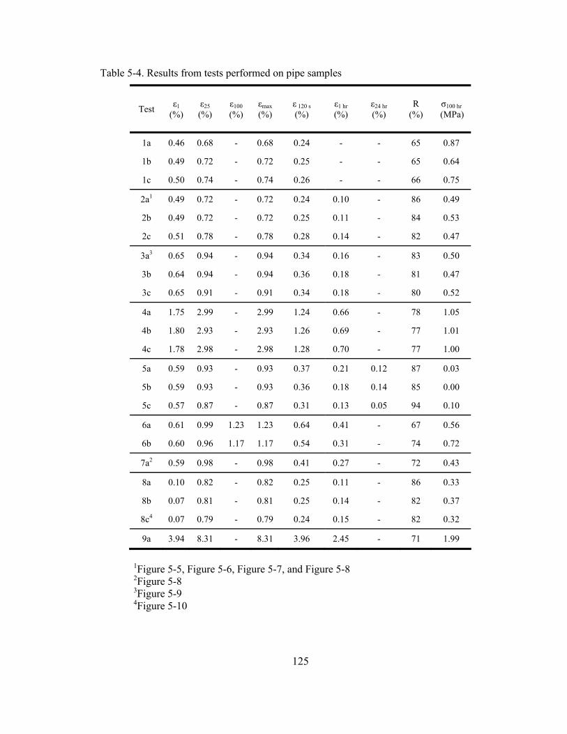
125

Table 5-4. Results from tests performed on pipe samples

Test ε1 (%)

ε25 (%)

ε100 (%)

εmax (%)

ε 120 s (%)

ε1 hr (%)

ε24 hr (%)

R (%)

σ100 hr

(MPa)

1a 0.46 0.68 - 0.68 0.24 - - 65 0.87

1b 0.49 0.72 - 0.72 0.25 - - 65 0.64

1c 0.50 0.74 - 0.74 0.26 - - 66 0.75

2a1 0.49 0.72 - 0.72 0.24 0.10 - 86 0.49

2b 0.49 0.72 - 0.72 0.25 0.11 - 84 0.53

2c 0.51 0.78 - 0.78 0.28 0.14 - 82 0.47

3a3 0.65 0.94 - 0.94 0.34 0.16 - 83 0.50

3b 0.64 0.94 - 0.94 0.36 0.18 - 81 0.47

3c 0.65 0.91 - 0.91 0.34 0.18 - 80 0.52

4a 1.75 2.99 - 2.99 1.24 0.66 - 78 1.05

4b 1.80 2.93 - 2.93 1.26 0.69 - 77 1.01

4c 1.78 2.98 - 2.98 1.28 0.70 - 77 1.00

5a 0.59 0.93 - 0.93 0.37 0.21 0.12 87 0.03

5b 0.59 0.93 - 0.93 0.36 0.18 0.14 85 0.00

5c 0.57 0.87 - 0.87 0.31 0.13 0.05 94 0.10

6a 0.61 0.99 1.23 1.23 0.64 0.41 - 67 0.56

6b 0.60 0.96 1.17 1.17 0.54 0.31 - 74 0.72

7a2 0.59 0.98 - 0.98 0.41 0.27 - 72 0.43

8a 0.10 0.82 - 0.82 0.25 0.11 - 86 0.33

8b 0.07 0.81 - 0.81 0.25 0.14 - 82 0.37

8c4 0.07 0.79 - 0.79 0.24 0.15 - 82 0.32

9a 3.94 8.31 - 8.31 3.96 2.45 - 71 1.99

1Figure 5-5, Figure 5-6, Figure 5-7, and Figure 5-8 2Figure 5-8 3Figure 5-9 4Figure 5-10

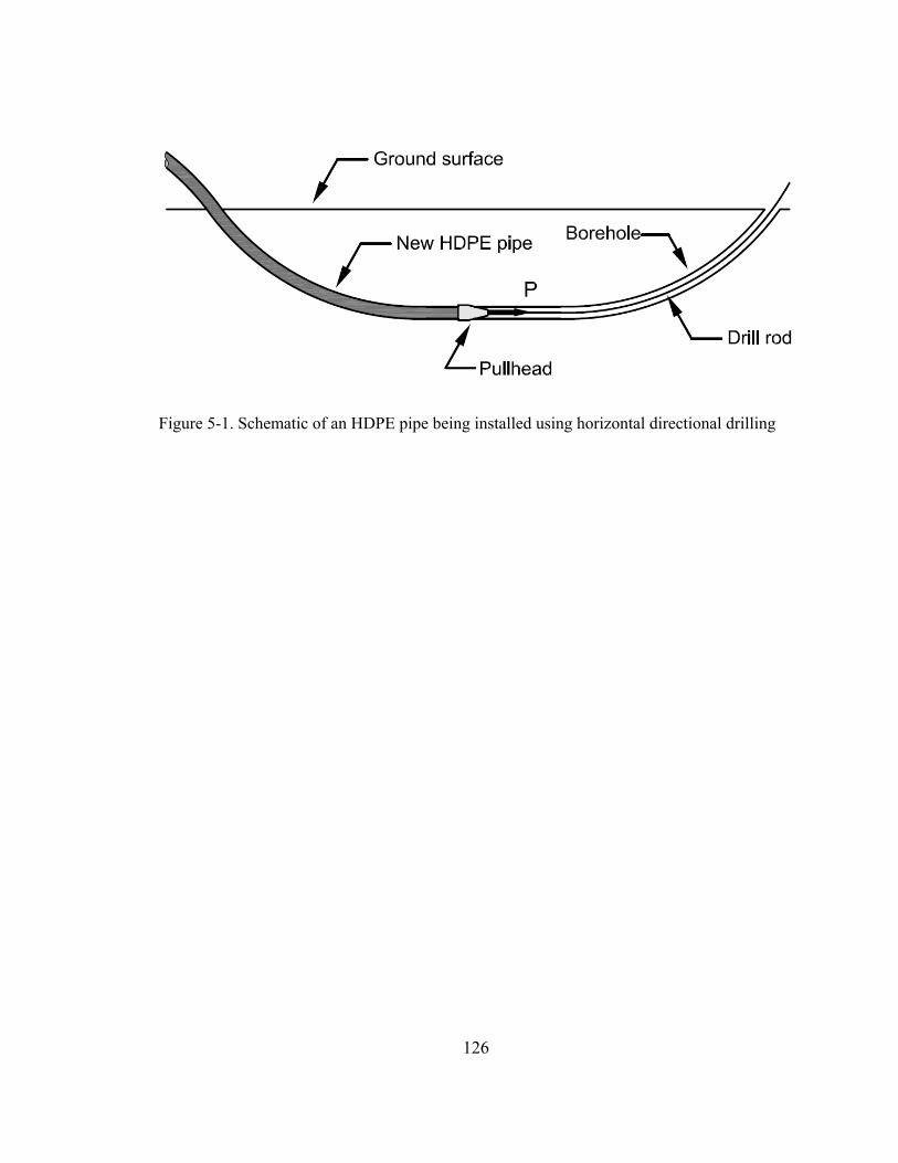
126

Figure 5-1. Schematic of an HDPE pipe being installed using horizontal directional drilling

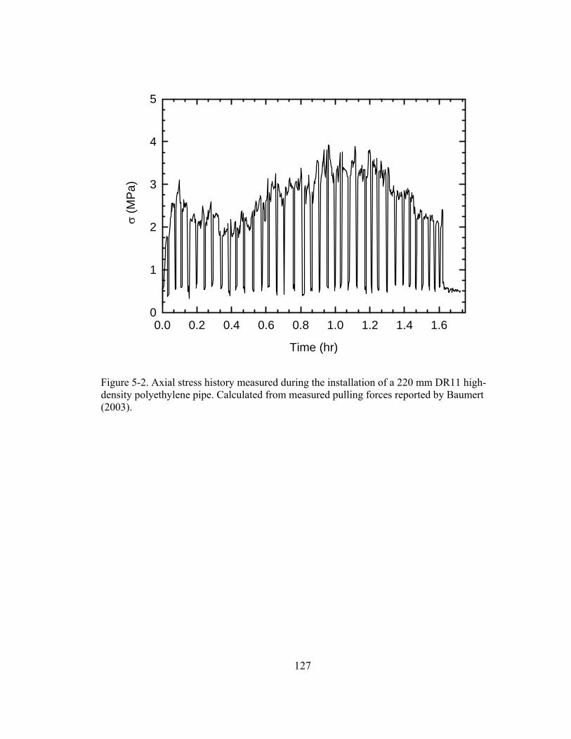
127

Time (hr)

0.0 0.2 0.4 0.6 0.8 1.0 1.2 1.4 1.6

σ (M

Pa)

0

1

2

3

4

5

Figure 5-2. Axial stress history measured during the installation of a 220 mm DR11 high-density polyethylene pipe. Calculated from measured pulling forces reported by Baumert (2003).

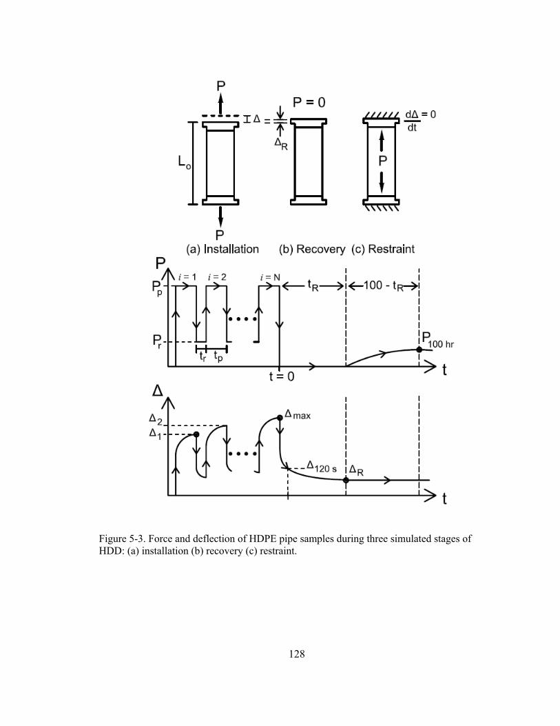
128

Figure 5-3. Force and deflection of HDPE pipe samples during three simulated stages of HDD: (a) installation (b) recovery (c) restraint.

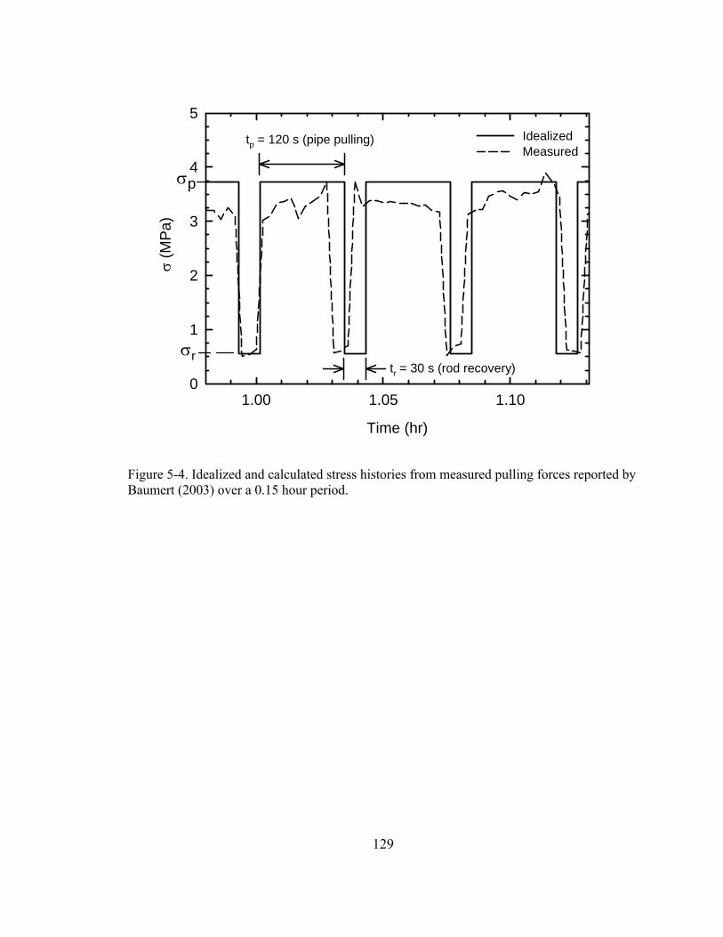
129

Time (hr)

1.00 1.05 1.10

σ (M

Pa)

0

1

2

3

4

5IdealizedMeasured

tp = 120 s (pipe pulling)

σp

σr tr = 30 s (rod recovery)

Figure 5-4. Idealized and calculated stress histories from measured pulling forces reported by Baumert (2003) over a 0.15 hour period.

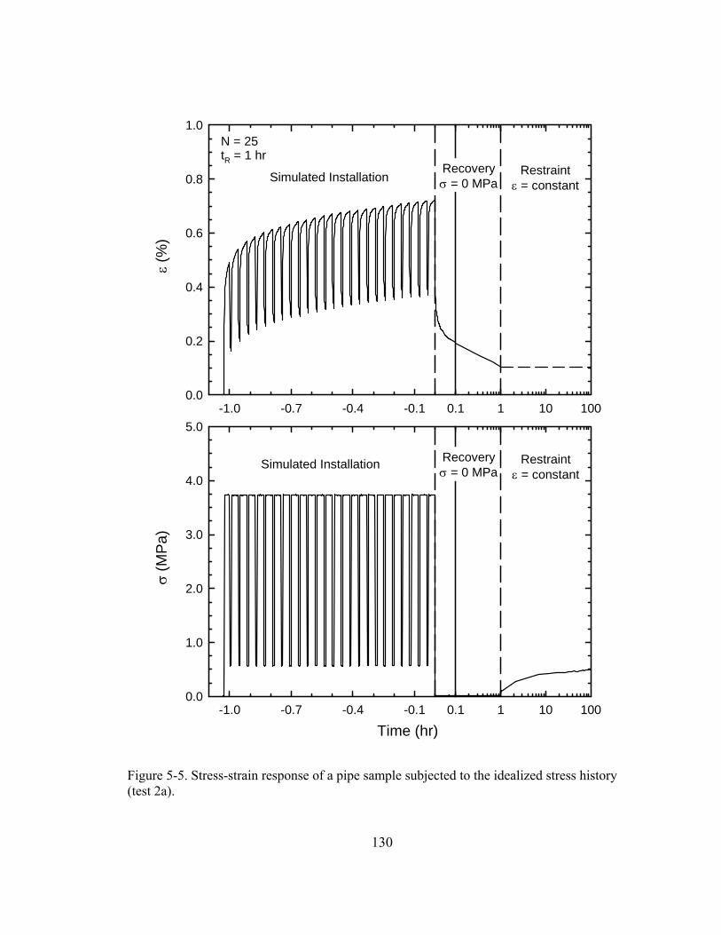
130

0.1 1 10 100-1.0 -0.7 -0.4 -0.1

ε (%

)

0.0

0.2

0.4

0.6

0.8

1.0

0.1 1 10 100

Time (hr)-1.0 -0.7 -0.4 -0.1

σ (M

Pa)

0.0

1.0

2.0

3.0

4.0

5.0

Simulated InstallationRecoveryσ = 0 MPa

Restraintε = constant

Recoveryσ = 0 MPa

Restraintε = constant

N = 25tR = 1 hr

Simulated Installation

Figure 5-5. Stress-strain response of a pipe sample subjected to the idealized stress history (test 2a).

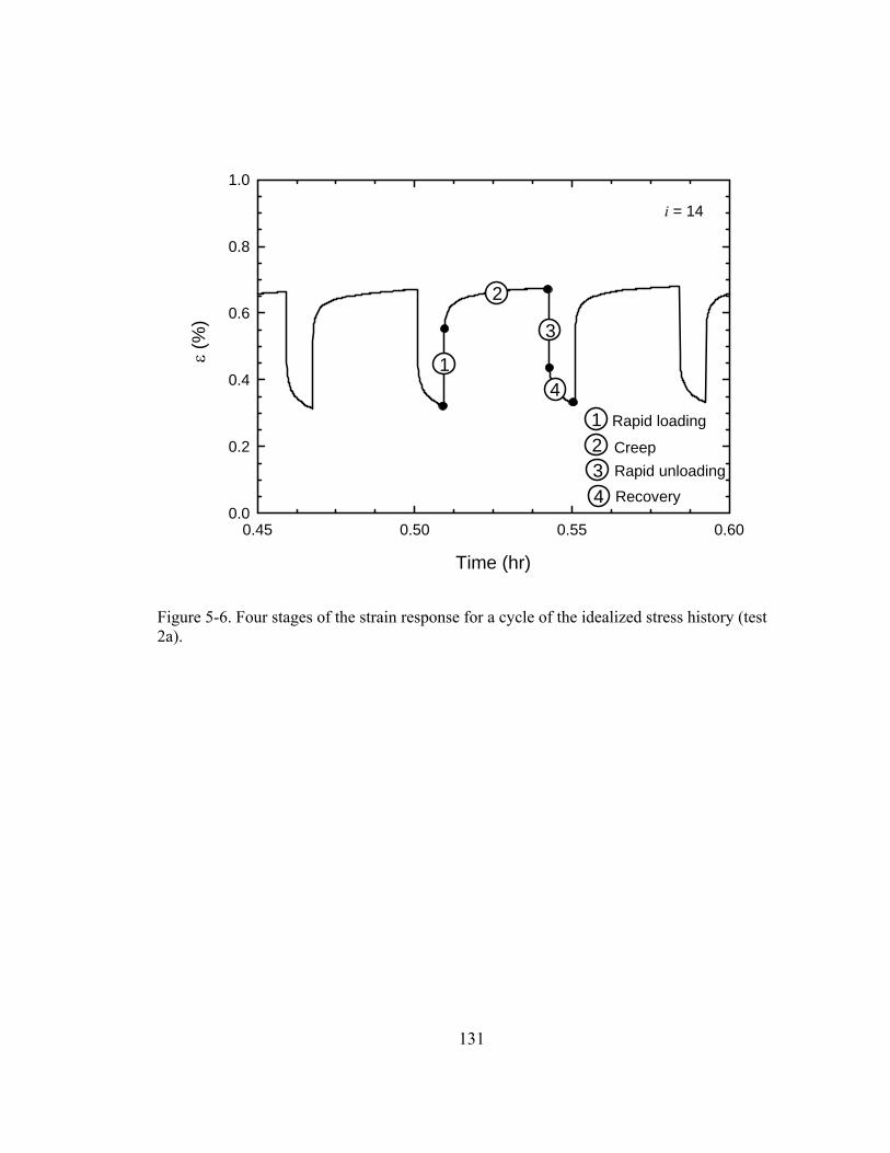
131

Time (hr)

0.45 0.50 0.55 0.60

ε (%

)

0.0

0.2

0.4

0.6

0.8

1.0

1

2

3

4

Recovery

1234

Rapid unloadingCreep

Rapid loading

i = 14

Figure 5-6. Four stages of the strain response for a cycle of the idealized stress history (test 2a).

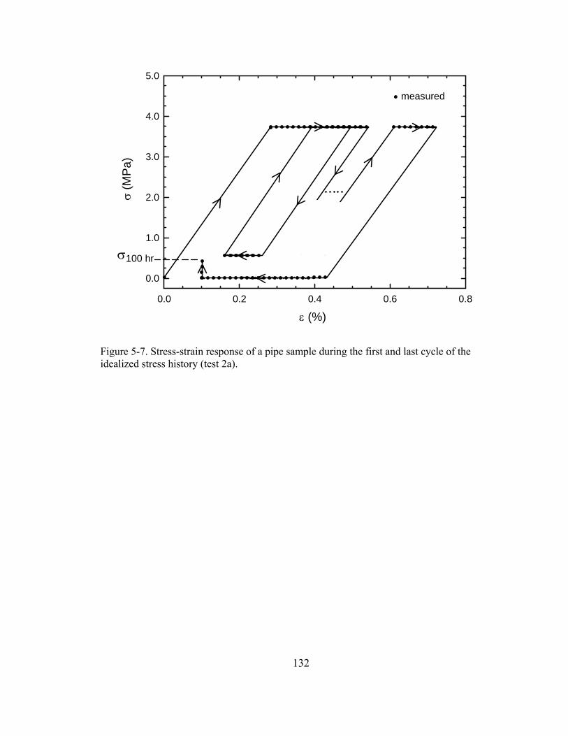
132

ε (%)0.0 0.2 0.4 0.6 0.8

σ (M

Pa)

0.0

1.0

2.0

3.0

4.0

5.0

σ100 hr

measured

Figure 5-7. Stress-strain response of a pipe sample during the first and last cycle of the idealized stress history (test 2a).

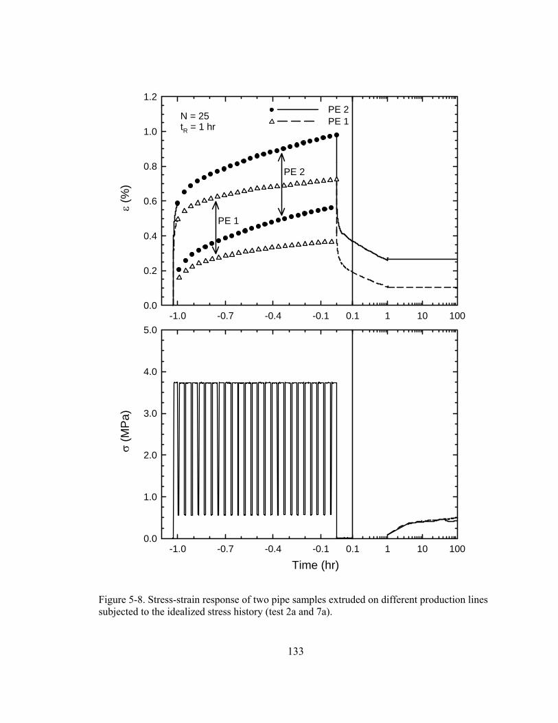
133

PE 2PE 1

0.1 1 10 100-1.0 -0.7 -0.4 -0.1

ε (%

)

0.0

0.2

0.4

0.6

0.8

1.0

1.2

0.1 1 10 100

Time (hr)-1.0 -0.7 -0.4 -0.1

σ (M

Pa)

0.0

1.0

2.0

3.0

4.0

5.0

N = 25tR = 1 hr

PE 1

PE 2

Figure 5-8. Stress-strain response of two pipe samples extruded on different production lines subjected to the idealized stress history (test 2a and 7a).

134

0.1 1 10 100-1.0 -0.7 -0.4 -0.1

ε (%

)

0.0

0.2

0.4

0.6

0.8

1.0

0.1 1 10 100

Time (hr)

-1.0 -0.7 -0.4 -0.1

σ (M

Pa)

0.0

1.0

2.0

3.0

4.0

5.0

N = 13tR = 1 hr

Figure 5-9. Stress-strain response of a pipe sample subjected to a modified stress history to simulate an HDD installation with longer drill rods (test 3a).

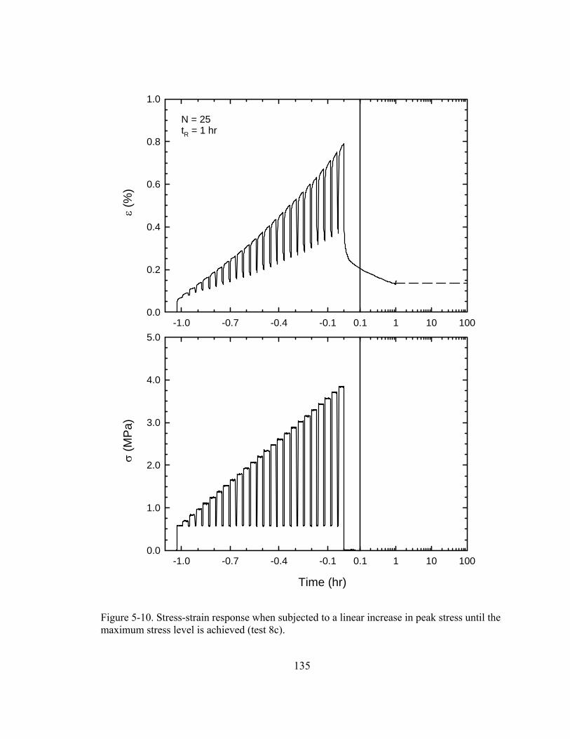
135

0.1 1 10 100-1.0 -0.7 -0.4 -0.1

ε (%

)

0.0

0.2

0.4

0.6

0.8

1.0

0.1 1 10 100

Time (hr)

-1.0 -0.7 -0.4 -0.1

σ (M

Pa)

0.0

1.0

2.0

3.0

4.0

5.0

N = 25tR = 1 hr

Figure 5-10. Stress-strain response when subjected to a linear increase in peak stress until the maximum stress level is achieved (test 8c).

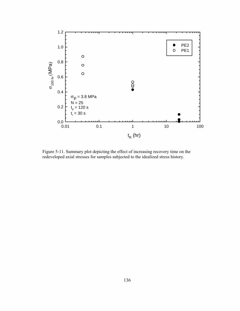
136

tR (hr)

0.01 0.1 1 10 100

σ 100

hr ( M

Pa)

0.0

0.2

0.4

0.6

0.8

1.0

1.2

σp = 3.8 MPaN = 25tp = 120 str = 30 s

PE2PE1

Figure 5-11. Summary plot depicting the effect of increasing recovery time on the redeveloped axial stresses for samples subjected to the idealized stress history.

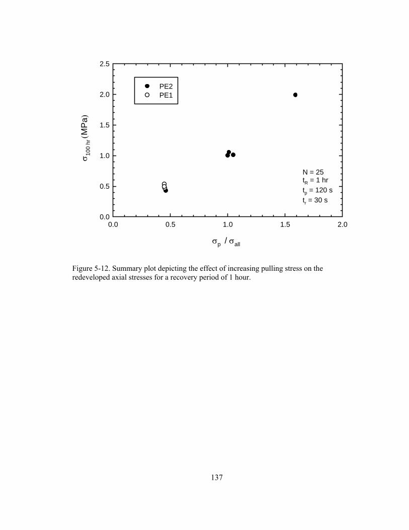
137

σp / σall

0.0 0.5 1.0 1.5 2.0

σ 100

hr ( M

Pa)

0.0

0.5

1.0

1.5

2.0

2.5

N = 25tR = 1 hrtp = 120 str = 30 s

PE2PE1

Figure 5-12. Summary plot depicting the effect of increasing pulling stress on the redeveloped axial stresses for a recovery period of 1 hour.

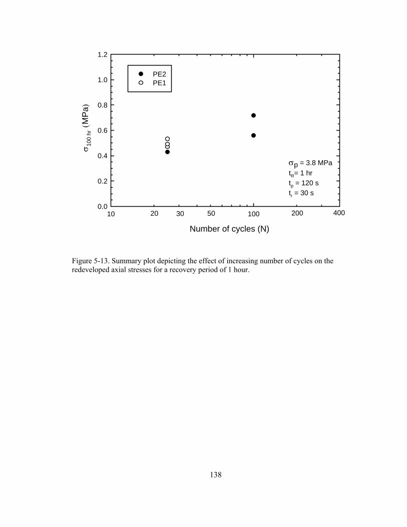
138

Number of cycles (N)

10 100

σ 100

hr (

MPa

)

0.0

0.2

0.4

0.6

0.8

1.0

1.2

PE2PE1

σp = 3.8 MPatR= 1 hrtp = 120 str = 30 s

40020030 5020

Figure 5-13. Summary plot depicting the effect of increasing number of cycles on the redeveloped axial stresses for a recovery period of 1 hour.

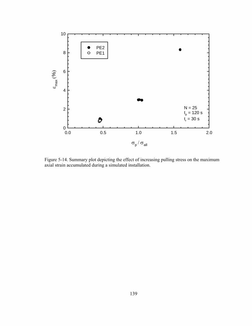
139

σp / σall

0.0 0.5 1.0 1.5 2.0

ε max

( %)

0

2

4

6

8

10

N = 25tp = 120 str = 30 s

PE2PE1

Figure 5-14. Summary plot depicting the effect of increasing pulling stress on the maximum axial strain accumulated during a simulated installation.

140

Chapter 6

Effectiveness of viscoelastic models for prediction of tensile axial

strains during cyclic loading of high-density polyethylene

6.1 Introduction

Polymer pipes, typically high-density polyethylene (HDPE), are commonly installed using

horizontal directional drilling. Horizontal directional drilling (HDD) is a trenchless

construction technique used to install underground services with minimal surface disruption

and disturbance (e.g. see ASTM F1962). A horizontal borehole is created underground with a

drill bit and a series of reamers to enable a pipe to be pulled into place (Figure 6-1). The soil

and rock cuttings are removed with a drilling fluid (bentonite mixture) that is pumped from

the borehole. A drill string, comprised of multiple drill rods, is used to pull the new pipe

through the borehole. The drill rig pulls on the drill string in a series of steps, as each

successive rod in the drill string is recovered (pulled back into the drill machine and

removed). This action generates cyclic axial tensile forces on the pipe that lead to tensile

axial strains. After installation, the pipe is unloaded and the elastic portion of the axial strains

begin to recover in a time dependent manner.

Cyclic axial force histories were measured during HDD installations by Baumert

(2003). It was shown that during each cycle, peak axial force values correspond to the tensile

force applied as the pipe is pulled through the borehole and the residual force values

correspond to the force applied as each successive drill rod is removed. Pulling force

equations have been proposed to estimate the maximum pulling force for a particular

installation, Baumert and Allouche (2002). The estimated pulling force is compared to

allowable limits to ensure the tensile axial stresses do not exceed the short-term yield

141

capacity of the pipe (ASTM F1804; AWWA M55). However, a more detailed investigation

of the axial stresses and strains imposed during and after an HDD installation is required to

quantify the effect of cyclic loading on the maximum axial strain that develops during

installation, and the long term performance of high-density polyethylene pipe after it is pulled

into place.

The objective of this chapter is to evaluate the ability of existing numerical models to

calculate the cyclic strain history of HDPE pipe during an HDD installation and to provide an

investigation into the parameters affecting the magnitude of these strains. The results from

the numerical models are compared against results from the experiments conducted on pipe

samples in Chapter 5. The ability of existing linear and nonlinear viscoelastic models (Moore

and Hu, 1996; Zhang and Moore, 1997b) to calculate the axial strain measured during those

simulated HDD installations is evaluated.

6.2 Experimental details

Laboratory simulations of an HDD installation were performed using isolated (i.e. not in

contact with soil) HDPE pipe samples to evaluate the effectiveness of existing numerical

models to calculate the strain response of HDPE both during and immediately after an HDD

installation. Intact pipe samples were tested rather than coupons or cylinders to eliminate

potential sample disturbance when specimens are cut from a pipe wall, such as release of

manufacturing induced residual stress (shown in Chapter 4).

The pipe samples tested had an average outside diameter of 167.5 mm and an average

wall thickness of 10.5 mm. A sample length of 500 mm was selected, based on numerical

analysis, to eliminate end effects caused by the standard stub end fittings welded to the ends

of the pipe sample (shown in Figure 6-2). Samples were tested at 23°C.

142

The axial boundary conditions for the experiments are shown in Figure 6-2. Tensile

forces (P) were applied through steel flanges bolted onto the stub ends and measured using an

external load cell accurate to ± 75 N. The corresponding deflections (Δ) were measured (±

0.01 mm) using two linear potentiometers mounted outside the pipe. The measured P and Δ

were used to calculate stress (σ) and strain (ε) based on the original cross-sectional area (A)

and gage length (L) of the sample. The gage length was determined in a separate experiment,

with specific details provided in Appendix E.

In terms of the radial boundary conditions, the exterior surface of the pipe was free

from shear stresses and radial pressure. These conditions differ from real installation

conditions (i.e. where shear stresses and radial pressures are generated by contact with the

surrounding soil and drilling fluid during installation). However, to evaluate the existing

viscoelastic models for HDPE, the axial response of the pipe was isolated.

6.2.1 Idealized stress history

To simulate the dominant features of an HDD installation, an idealized cyclic stress history

was developed and imposed on the isolated pipe samples. The idealized stress history was

developed using a particular pulling force history measured in the field as guidance

(Baumert, 2003). The field data was measured just behind the pullhead and consequently the

idealized stress history simulates the loading applied to the section of HDPE pipe at this

location, shown to be the most heavily loaded section of pipe during installation by Chehab

and Moore (2006).

A portion of the measured cyclic stress history used in developing the idealized stress

history is given in Figure 6-3. Peak axial stress values (σp) correspond to the tensile stress

applied as the pipe is actively pulled through the borehole (neglecting bending effects which

143

are small) and recovery stress values (σr) correspond to the stress applied as pulling is

temporarily interrupted to remove a segment of drill rod. During periods of rod removal the

pipe is not completely unloaded as friction is mobilized between the drill string or the pipe

and the drilling fluid surrounding them in the borehole.

A cycle of the idealized stress history (Figure 6-3) consists of the application of σp

held for a period of 120 seconds followed by instantaneous unloading to σr held until the

beginning of the next cycle (30 seconds). While pulling force histories during actual HDD

installations are complex and variable, the idealized cyclic stress history captures the key

elements of pulling and releasing the pipe until it is installed.

6.2.2 Tests conducted

The idealized stress history was imposed for 25 cycles (simulating a 75 m installation where

3 m long drill rods were used) followed by a period of strain recovery to quantify the strain

response during and after installation. The experimental results are denoted T-1 in Table 6-1.

Three pipe samples (T-1-1, T-1-2, and T-1-3) were subjected to the idealized stress history

shown in Figure 6-3 to evaluate result repeatability. Results from additional tests performed

on HDPE pipe samples were reported in Chapter 5.

6.3 Numerical model details

6.3.1 Existing numerical models

While a number of sophisticated time dependent models have been developed for HDPE over

the past decade, model parameters are generally not available for analysis of specific HDPE

products since evaluation of those parameters generally requires an expensive series of

constitutive tests followed by back-calculations that are beyond the abilities of most

practitioners (for example, the series of constant strain-rate tests required for the viscoplastic

144

model of Zhang and Moore 1997b, and the isotach model of Dhar et al. 2006). Exceptions

are the viscoelastic models based on curve fits to simple creep tests. These tests are generally

the easiest to perform, and are commonly available from product manufacturers.

Linear viscoelastic (LVE) models (e.g. Moore and Hu, 1996), as well as the nonlinear

viscoelastic (NVE) models used at higher stresses levels (e.g. Zhang and Moore, 1997b),

need only the spring stiffnesses to be determined so the calculated strain response fits the

creep data. The linear viscoelastic model of Moore and Hu (1996) features the multi-Kelvin

elements shown in Figure 6-4. One independent spring in conjunction with nine Kelvin

elements in series (each consisting of a spring and dashpot in parallel) was implemented to

model the HDPE over long time periods (minutes to years). The independent spring predicts

the instantaneous response while each Kelvin element is used to capture the time-dependant

behaviour over one cycle of log time. The rheological parameters (i.e. modulus of the

independent spring, moduli for the Kelvin springs, and viscosities for the Kelvin dashpots)

are constants, and were developed using a curve fitting exercise to the relaxation test data of

Chua (1986). These particular parameters are given in Figure 6-4.

The linear viscoelastic model of Moore and Hu (1996) was extended by Zhang and

Moore (1997b) to include nonlinear rheology. The results from uniaxial creep tests on

samples cut from thick-walled HDPE pipe were used by Zhang and Moore (1997b) to

formulate a viscoelastic model where the parameters (moduli or viscosities) for one spring

and six Kelvin elements in series are defined as functions of stress such that:

Eo = aoexp(-a1σ3) [6-1]

E1 = bo + b1exp(-σ / b2) [6-2]

τ1 = coexp(-c1 + c2σ + c3 σ2 – c4 σ3) [6-3]

145

where: ao = 1400 MPa, a1 = 4.65 x 10-5 MPa-3, bo = 260 MPa, b1 = 19545 MPa, b2 = 8.3 MPa,

co = 8.64 x 102 s, c1 = 10.5, c2 = 0.218 MPa-1, c3 = 1.37 x 10-3 MPa-2, and c4 = 1.66 x 10-4

MPa-3.

Since viscoelastic models feature the two most important characteristics of the cyclic

response expected when HDPE is subjected to the idealized stress history shown in Figure 6-

3 (strain accumulation with time while at the maximum stress level, and strain recovery

following unloading to the minimum value of cyclic stress), the viscoelastic models of Moore

and Hu (1996) and Zhang and Moore (1997b) were used to investigate the response of the

HDPE pipe under the cyclic loading history associated with HDD installation. Parameters for

both of these models are available for the same HDPE pipe material tested in the laboratory,

making them more attractive than other viscoelastic constitutive models (e.g. Ellyin et. al.

2007)

6.3.2 Model geometry

Numerical analysis featured evaluation of the behaviour of HDPE using an isolated block,

since for a prismatic structure under uniform, uniaxial stress the constitutive response defined

in terms of stress and strain is independent of geometry. The model geometry is given in

Figure 6-5. The mesh consisted of two six nodded triangles with smooth rigid boundaries

along lines x = 0 and y = 0 such that the node located at the origin (x = 0 and y = 0) was fixed

in both the x and y directions. Loads (P) were imposed on the block at the nodes in the

configuration shown in Figure 6-5.

146

6.4 Results

6.4.1 Laboratory measurements

Figure 6-6 gives the strain history measured in the laboratory of a pipe sample subjected to

the idealized stress history (T-1-1) and the post-installation strain response. When t = 0, the

simulated installation is complete and the post-installation period begins. Tensile strains are

taken as positive. The results in Figure 6-6 show that for each load cycle the axial strain

progressively accumulates. In fact, the axial strain at the end of the first cycle (ε1) was 0.49%

increasing to 0.72% after 25 cycles (ε25). During strain recovery, axial strain reduced from

0.72% (at t=0) to 0.19% after 0.1 hours (εR=0.1) with recovery continuing to 0.10% after 1

hour (εR=1).

Figure 6-6 suggests that strain accumulation during pulling appears to be dominated

by creep under the maximum pulling stress σp, while viscoelastic strain recovery leads to

substantial reductions in axial strain during load reduction to the minimum stress σr. The

performance of calculations based on linear and nonlinear viscoelastic modeling of the HDPE

is therefore explored in the sections that follow.

6.4.2 Numerical model evaluation

Figure 6-7 compares the viscoelastic calculations for the LVE (C-1-1) and NVE (C-1-2)

models to the measured results (T-1-1) where the maximum and minimum strain for each of

the 25 cycles is plotted as points and continuous data as a line (sample input files are

provided in Appendix G for these models). The results in Figure 6-7 show that both models

provide reasonable estimates of the maximum strain levels during installation. However,

maximum strains were underestimated by the LVE model and overestimated by the NVE

model. For example, the LVE model underestimated ε25 by a strain of 0.04% and the NVE

model overestimated ε25 by a strain of 0.04%. None of the axial strain levels exceed 1%, and

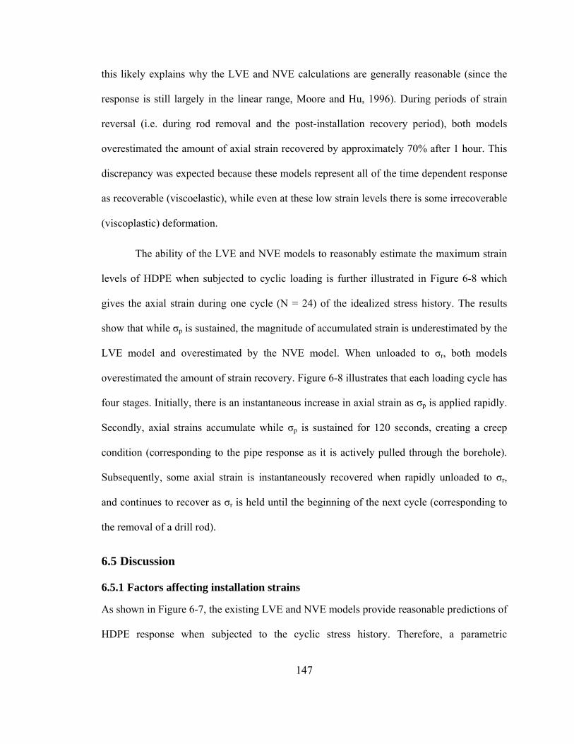
147

this likely explains why the LVE and NVE calculations are generally reasonable (since the

response is still largely in the linear range, Moore and Hu, 1996). During periods of strain

reversal (i.e. during rod removal and the post-installation recovery period), both models

overestimated the amount of axial strain recovered by approximately 70% after 1 hour. This

discrepancy was expected because these models represent all of the time dependent response

as recoverable (viscoelastic), while even at these low strain levels there is some irrecoverable

(viscoplastic) deformation.

The ability of the LVE and NVE models to reasonably estimate the maximum strain

levels of HDPE when subjected to cyclic loading is further illustrated in Figure 6-8 which

gives the axial strain during one cycle (N = 24) of the idealized stress history. The results

show that while σp is sustained, the magnitude of accumulated strain is underestimated by the

LVE model and overestimated by the NVE model. When unloaded to σr, both models

overestimated the amount of strain recovery. Figure 6-8 illustrates that each loading cycle has

four stages. Initially, there is an instantaneous increase in axial strain as σp is applied rapidly.

Secondly, axial strains accumulate while σp is sustained for 120 seconds, creating a creep

condition (corresponding to the pipe response as it is actively pulled through the borehole).

Subsequently, some axial strain is instantaneously recovered when rapidly unloaded to σr,

and continues to recover as σr is held until the beginning of the next cycle (corresponding to

the removal of a drill rod).

6.5 Discussion

6.5.1 Factors affecting installation strains

As shown in Figure 6-7, the existing LVE and NVE models provide reasonable predictions of

HDPE response when subjected to the cyclic stress history. Therefore, a parametric

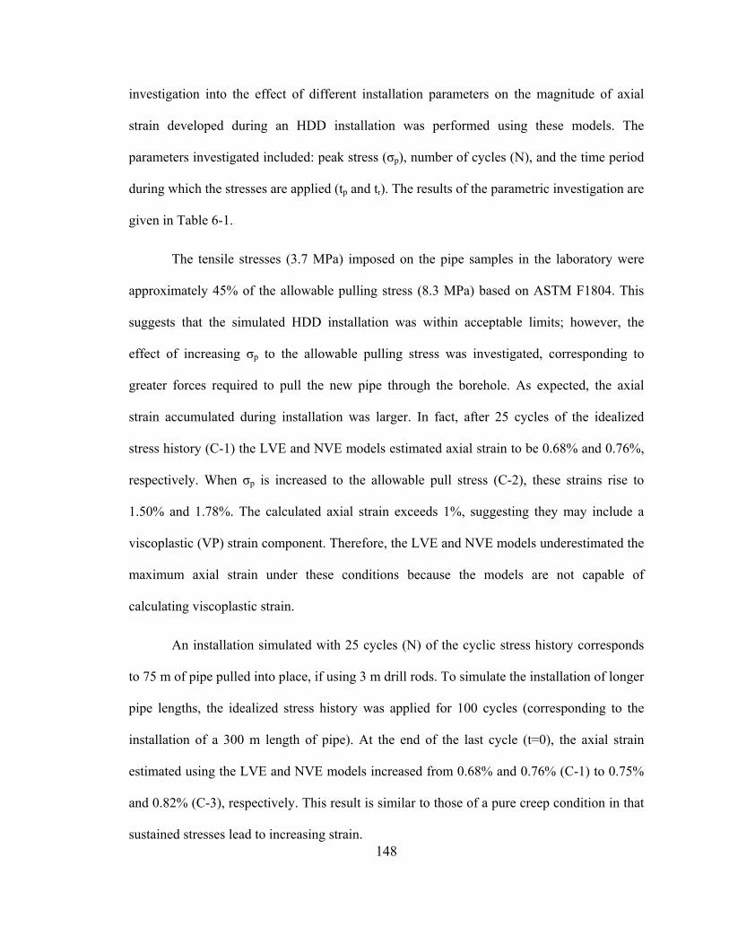
148

investigation into the effect of different installation parameters on the magnitude of axial

strain developed during an HDD installation was performed using these models. The

parameters investigated included: peak stress (σp), number of cycles (N), and the time period

during which the stresses are applied (tp and tr). The results of the parametric investigation are

given in Table 6-1.

The tensile stresses (3.7 MPa) imposed on the pipe samples in the laboratory were

approximately 45% of the allowable pulling stress (8.3 MPa) based on ASTM F1804. This

suggests that the simulated HDD installation was within acceptable limits; however, the

effect of increasing σp to the allowable pulling stress was investigated, corresponding to

greater forces required to pull the new pipe through the borehole. As expected, the axial

strain accumulated during installation was larger. In fact, after 25 cycles of the idealized

stress history (C-1) the LVE and NVE models estimated axial strain to be 0.68% and 0.76%,

respectively. When σp is increased to the allowable pull stress (C-2), these strains rise to

1.50% and 1.78%. The calculated axial strain exceeds 1%, suggesting they may include a

viscoplastic (VP) strain component. Therefore, the LVE and NVE models underestimated the

maximum axial strain under these conditions because the models are not capable of

calculating viscoplastic strain.

An installation simulated with 25 cycles (N) of the cyclic stress history corresponds

to 75 m of pipe pulled into place, if using 3 m drill rods. To simulate the installation of longer

pipe lengths, the idealized stress history was applied for 100 cycles (corresponding to the

installation of a 300 m length of pipe). At the end of the last cycle (t=0), the axial strain

estimated using the LVE and NVE models increased from 0.68% and 0.76% (C-1) to 0.75%

and 0.82% (C-3), respectively. This result is similar to those of a pure creep condition in that

sustained stresses lead to increasing strain.

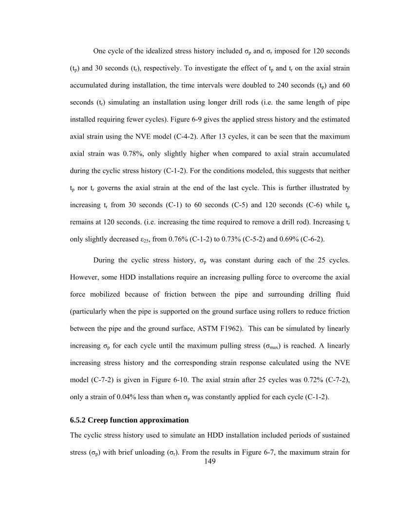
149

One cycle of the idealized stress history included σp and σr imposed for 120 seconds

(tp) and 30 seconds (tr), respectively. To investigate the effect of tp and tr on the axial strain

accumulated during installation, the time intervals were doubled to 240 seconds (tp) and 60

seconds (tr) simulating an installation using longer drill rods (i.e. the same length of pipe

installed requiring fewer cycles). Figure 6-9 gives the applied stress history and the estimated

axial strain using the NVE model (C-4-2). After 13 cycles, it can be seen that the maximum

axial strain was 0.78%, only slightly higher when compared to axial strain accumulated

during the cyclic stress history (C-1-2). For the conditions modeled, this suggests that neither

tp nor tr governs the axial strain at the end of the last cycle. This is further illustrated by

increasing tr from 30 seconds (C-1) to 60 seconds (C-5) and 120 seconds (C-6) while tp

remains at 120 seconds. (i.e. increasing the time required to remove a drill rod). Increasing tr

only slightly decreased ε25, from 0.76% (C-1-2) to 0.73% (C-5-2) and 0.69% (C-6-2).

During the cyclic stress history, σp was constant during each of the 25 cycles.

However, some HDD installations require an increasing pulling force to overcome the axial

force mobilized because of friction between the pipe and surrounding drilling fluid

(particularly when the pipe is supported on the ground surface using rollers to reduce friction

between the pipe and the ground surface, ASTM F1962). This can be simulated by linearly

increasing σp for each cycle until the maximum pulling stress (σmax) is reached. A linearly

increasing stress history and the corresponding strain response calculated using the NVE

model (C-7-2) is given in Figure 6-10. The axial strain after 25 cycles was 0.72% (C-7-2),

only a strain of 0.04% less than when σp was constantly applied for each cycle (C-1-2).

6.5.2 Creep function approximation

The cyclic stress history used to simulate an HDD installation included periods of sustained

stress (σp) with brief unloading (σr). From the results in Figure 6-7, the maximum strain for

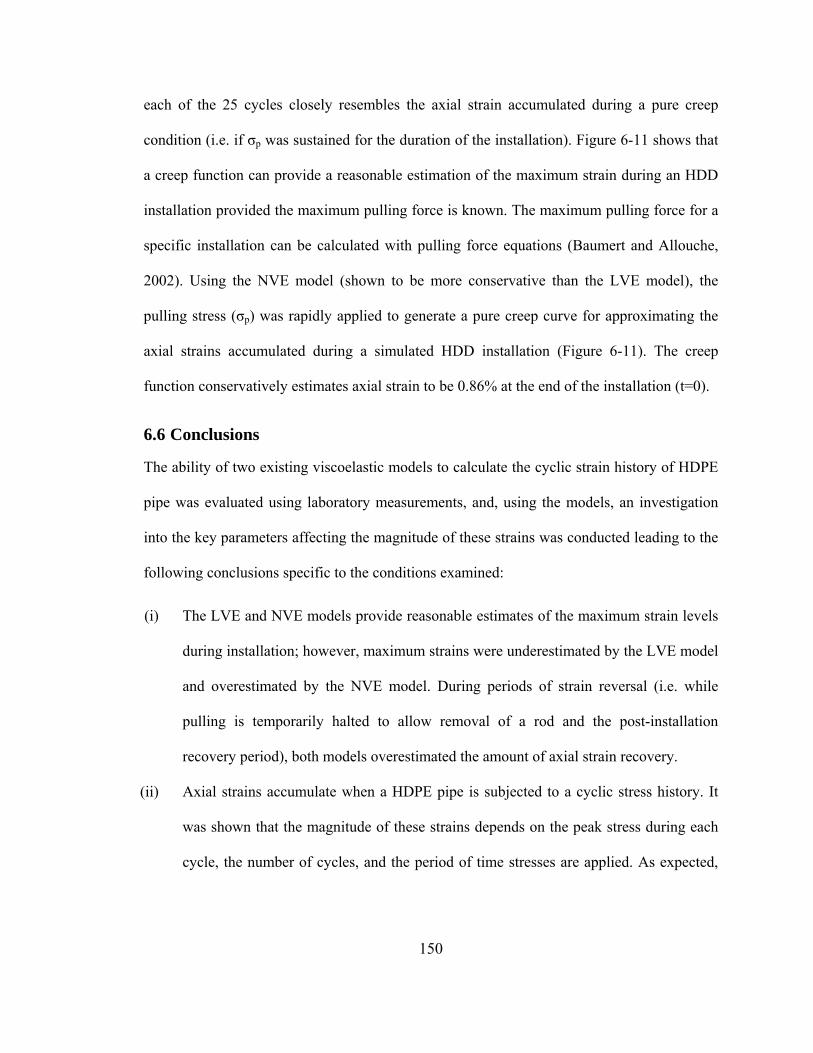
150

each of the 25 cycles closely resembles the axial strain accumulated during a pure creep

condition (i.e. if σp was sustained for the duration of the installation). Figure 6-11 shows that

a creep function can provide a reasonable estimation of the maximum strain during an HDD

installation provided the maximum pulling force is known. The maximum pulling force for a

specific installation can be calculated with pulling force equations (Baumert and Allouche,

2002). Using the NVE model (shown to be more conservative than the LVE model), the

pulling stress (σp) was rapidly applied to generate a pure creep curve for approximating the

axial strains accumulated during a simulated HDD installation (Figure 6-11). The creep

function conservatively estimates axial strain to be 0.86% at the end of the installation (t=0).

6.6 Conclusions

The ability of two existing viscoelastic models to calculate the cyclic strain history of HDPE

pipe was evaluated using laboratory measurements, and, using the models, an investigation

into the key parameters affecting the magnitude of these strains was conducted leading to the

following conclusions specific to the conditions examined:

(i) The LVE and NVE models provide reasonable estimates of the maximum strain levels

during installation; however, maximum strains were underestimated by the LVE model

and overestimated by the NVE model. During periods of strain reversal (i.e. while

pulling is temporarily halted to allow removal of a rod and the post-installation

recovery period), both models overestimated the amount of axial strain recovery.

(ii) Axial strains accumulate when a HDPE pipe is subjected to a cyclic stress history. It

was shown that the magnitude of these strains depends on the peak stress during each

cycle, the number of cycles, and the period of time stresses are applied. As expected,

151

increases in the peak stress and the number of cycles lead to increases in the maximum

axial strain, and these were quantified.

(iii) A creep function provides a conservative estimate of the maximum strain during an

HDD installation provided the maximum pulling force is known.

6.7 References

ASTM F 1804-08. Standard Practice for Determining Allowable Tensile Load for

Polyethylene (PE) Gas Pipe During Pull-In Installation. Annual Book of ASTM

Standards, ASTM.

ASTM F 1962-05 Standard Guide for Use of Maxi-Horizontal Directional Drilling for

Placement of Polyethylene Pipe or Conduit Under Obstacles, Including River Crossings.

Annual Book of ASTM Standards, ASTM.

AWWA M55. PE Pipe – Design and Installation (M55). American Water Works Association,

Denver, COL.

Baumert, M. E. and Allouche, E. N. 2002, Methods for estimating pipe pullback loads for

horizontal directional drilling crossings. Journal of Infrastructure Systems, ASCE, 8(1):

12-19.

Baumert, M.E. 2003. Experimental investigation of pulling loads and mud pressures during

horizontal directional drilling installations. PhD Thesis, The University of Western

Ontario, London, Ontario.

Chua, K.M. 1986. Time-dependent interaction of soil and flexible pipe. Ph.D. thesis, Texas A

& M University, College Station, Tex.

Chehab, A.G., Moore, I.D. 2006. A viscoelastic-viscoplastic constitutive model for high

density Polyethylene, Pipelines 2006, ASCE, Chicago, July-August, 7pp.

Dhar, A.S., Siddiquee, M.S.A, Tatsuoka F. and Noor, M.A. 2006. An isotach model for time

dependent behaviour of high density polyethylene. Paper 06-0952, 85th Annual

Meeting of Transportation Research Board, Washington D.C.

152

Ellyin, F., Vaziri, R., and Bigot, L. 2007. Predictions of two nonlinear viscoelastic

constitutive relations for polymers under multiaxial loadings. Polymer Engineering &

Science, 47(5), 593 – 607.

Moore, I.D. and Hu, F. 1996. Linear viscoelastic modeling of profiled high density

polyethylene pipe. Canadian Journal of Civil Engineering, 23(2): 395-407

Zhang, C., and Moore, I.D. 1997a. Nonlinear mechanical response of high density

polyethylene. Part I: Experimental investigation and model evaluation. Polymer

Engineering and Science, 37(2): 404-413

Zhang, C., and Moore, I.D. 1997b. Nonlinear mechanical response of high density

polyethylene. Part II: Uniaxial constitutive modeling. Polymer Engineering and Science,

37(2): 414-420

White, D.J., Take, W.A. and Bolton, M.D. 2003. Soil deformation measurement using

particle image velocimetry (PIV) and photogrammetry. Geotechnique 53 (7):619-631.

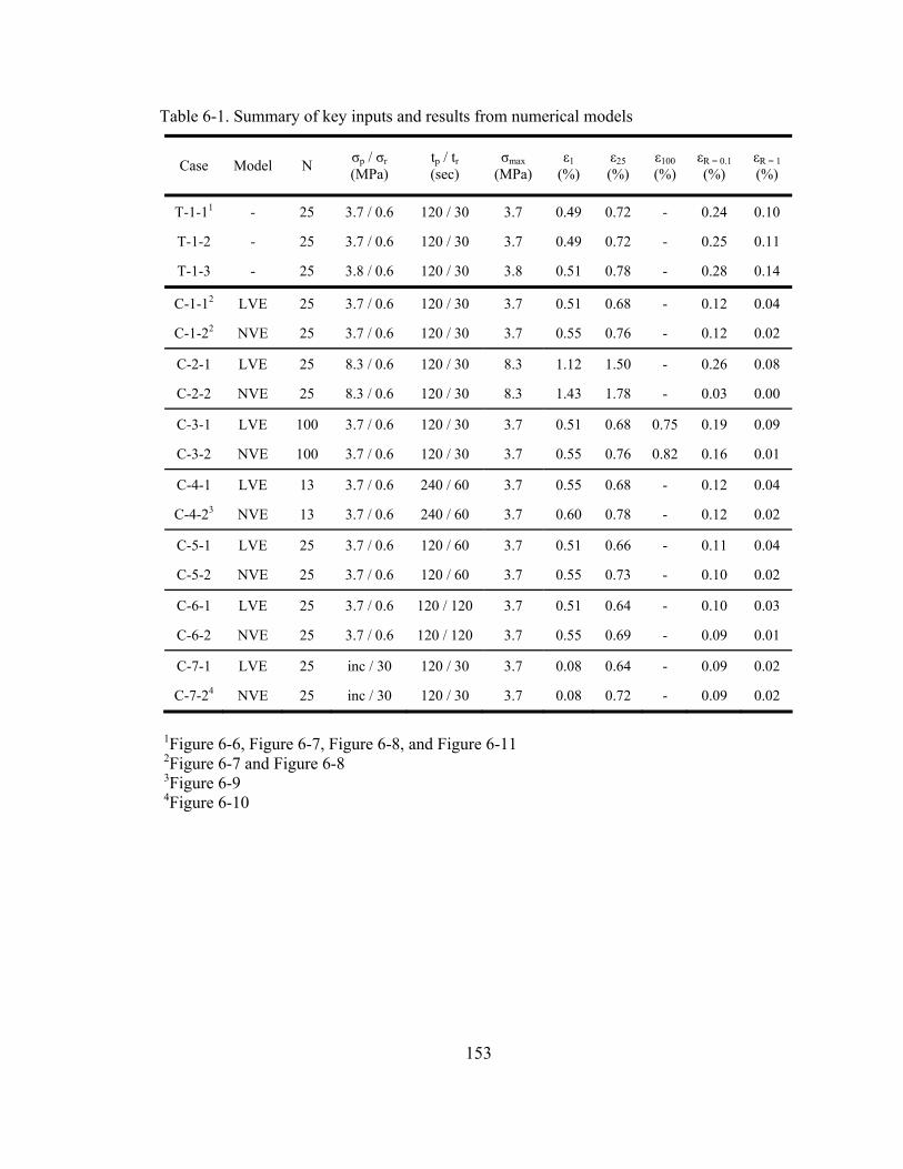
153

Table 6-1. Summary of key inputs and results from numerical models

Case Model N σp / σr (MPa)

tp / tr (sec)

σmax (MPa)

ε1 (%)

ε25 (%)

ε100 (%)

εR = 0.1 (%)

εR = 1 (%)

T-1-11 - 25 3.7 / 0.6 120 / 30 3.7 0.49 0.72 - 0.24 0.10

T-1-2 - 25 3.7 / 0.6 120 / 30 3.7 0.49 0.72 - 0.25 0.11

T-1-3 - 25 3.8 / 0.6 120 / 30 3.8 0.51 0.78 - 0.28 0.14

C-1-12 LVE 25 3.7 / 0.6 120 / 30 3.7 0.51 0.68 - 0.12 0.04

C-1-22 NVE 25 3.7 / 0.6 120 / 30 3.7 0.55 0.76 - 0.12 0.02

C-2-1 LVE 25 8.3 / 0.6 120 / 30 8.3 1.12 1.50 - 0.26 0.08

C-2-2 NVE 25 8.3 / 0.6 120 / 30 8.3 1.43 1.78 - 0.03 0.00

C-3-1 LVE 100 3.7 / 0.6 120 / 30 3.7 0.51 0.68 0.75 0.19 0.09

C-3-2 NVE 100 3.7 / 0.6 120 / 30 3.7 0.55 0.76 0.82 0.16 0.01

C-4-1 LVE 13 3.7 / 0.6 240 / 60 3.7 0.55 0.68 - 0.12 0.04

C-4-23 NVE 13 3.7 / 0.6 240 / 60 3.7 0.60 0.78 - 0.12 0.02

C-5-1 LVE 25 3.7 / 0.6 120 / 60 3.7 0.51 0.66 - 0.11 0.04

C-5-2 NVE 25 3.7 / 0.6 120 / 60 3.7 0.55 0.73 - 0.10 0.02

C-6-1 LVE 25 3.7 / 0.6 120 / 120 3.7 0.51 0.64 - 0.10 0.03

C-6-2 NVE 25 3.7 / 0.6 120 / 120 3.7 0.55 0.69 - 0.09 0.01

C-7-1 LVE 25 inc / 30 120 / 30 3.7 0.08 0.64 - 0.09 0.02

C-7-24 NVE 25 inc / 30 120 / 30 3.7 0.08 0.72 - 0.09 0.02

1Figure 6-6, Figure 6-7, Figure 6-8, and Figure 6-11 2Figure 6-7 and Figure 6-8 3Figure 6-9 4Figure 6-10

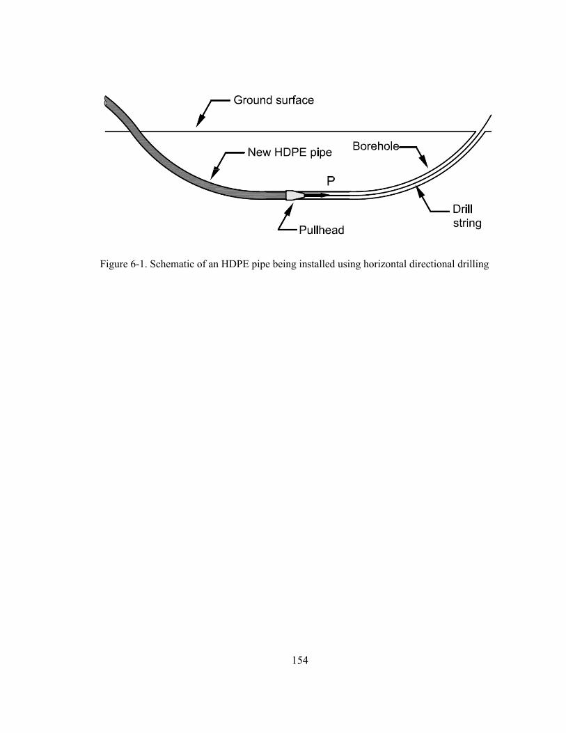
154

Figure 6-1. Schematic of an HDPE pipe being installed using horizontal directional drilling

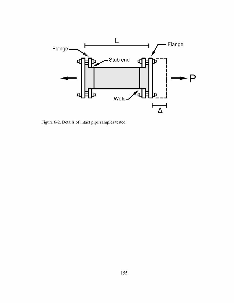
155

Figure 6-2. Details of intact pipe samples tested.

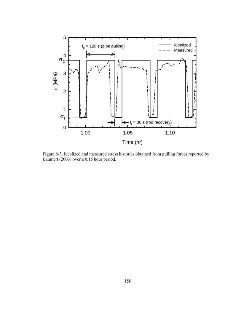
156

Time (hr)

1.00 1.05 1.10

σ (M

Pa)

0

1

2

3

4

5IdealizedMeasured

tp = 120 s (pipe pulling)

σp

σr tr = 30 s (rod recovery)

Figure 6-3. Idealized and measured stress histories obtained from pulling forces reported by Baumert (2003) over a 0.15 hour period.

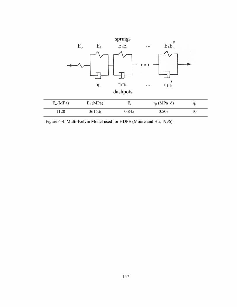
157

Eo (MPa) E1 (MPa) Er η1 (MPa ·d) ηr

1120 3615.6 0.845 0.503 10

Figure 6-4. Multi-Kelvin Model used for HDPE (Moore and Hu, 1996).

Eo E1 E1Er E1Er 8

η1 η1ηr η1ηr 8

springs

dashpots

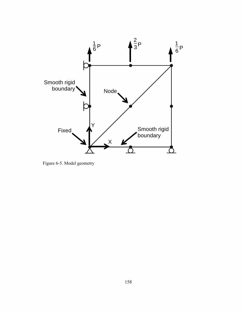
158

Figure 6-5. Model geometry

Smooth rigid boundary

Fixed Smooth rigid boundary

X

Y

Node

1 6 _

P 2 _

P3 1 6 _ P

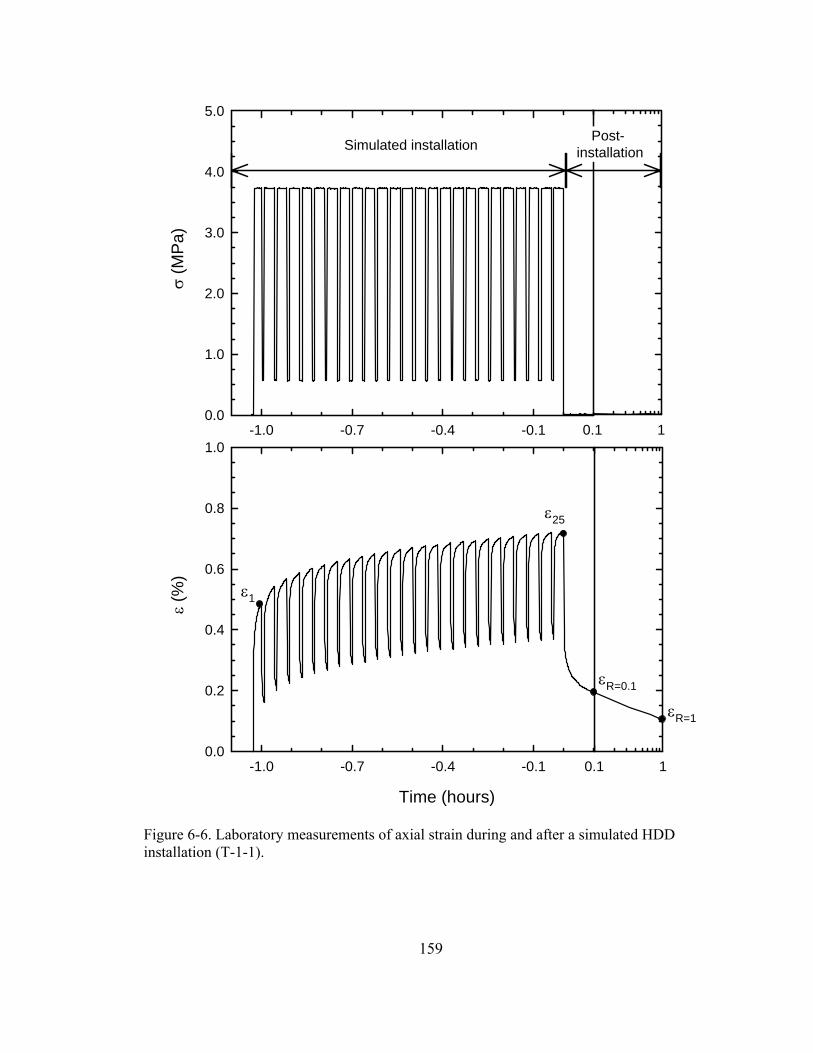
159

0.1 1

Time (hours)

-1.0 -0.7 -0.4 -0.1

ε (%

)

0.0

0.2

0.4

0.6

0.8

1.00.1 1-1.0 -0.7 -0.4 -0.1

σ (M

Pa)

0.0

1.0

2.0

3.0

4.0

5.0

ε1

ε25

εR=0.1

εR=1

Simulated installation Post- installation

Figure 6-6. Laboratory measurements of axial strain during and after a simulated HDD installation (T-1-1).

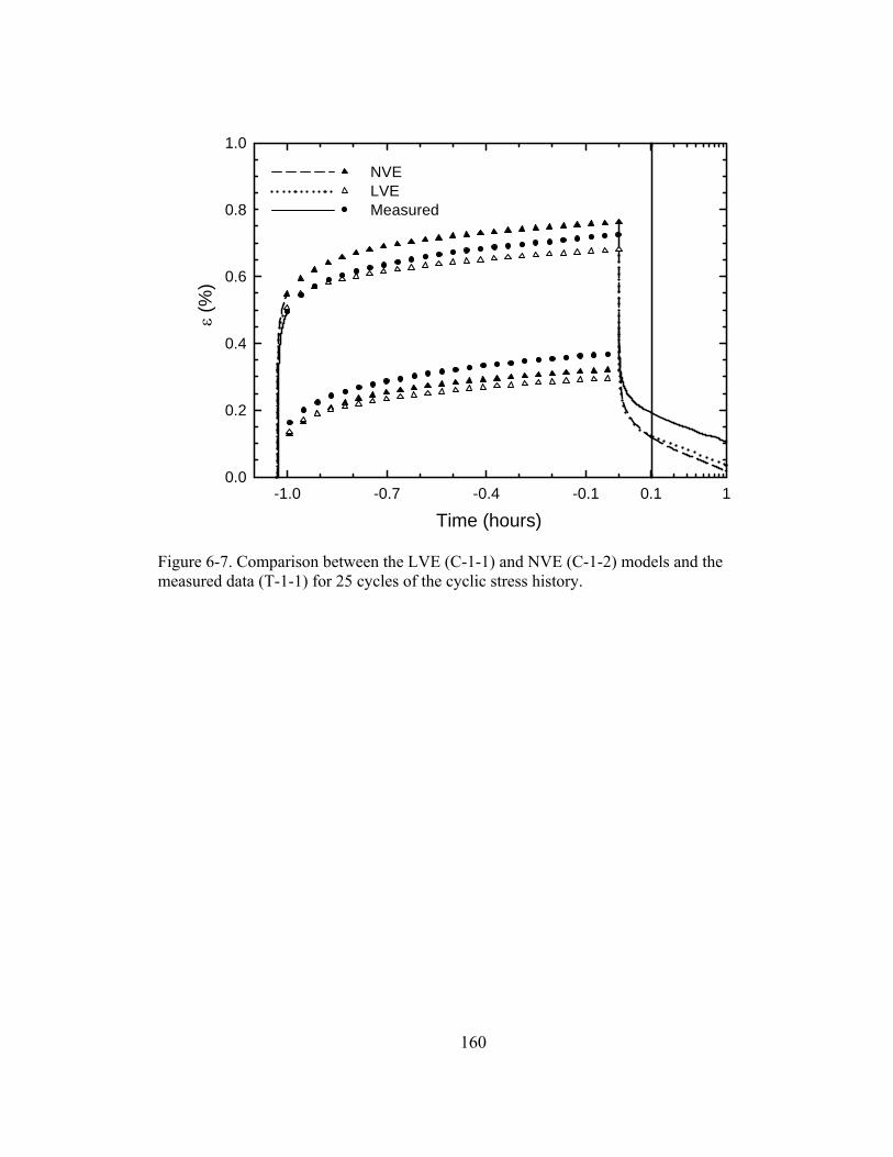
160

0.1 1

Time (hours)-1.0 -0.7 -0.4 -0.1

ε (%

)

0.0

0.2

0.4

0.6

0.8

1.0

NVELVEMeasured

NVELVEMeasured

Figure 6-7. Comparison between the LVE (C-1-1) and NVE (C-1-2) models and the measured data (T-1-1) for 25 cycles of the cyclic stress history.

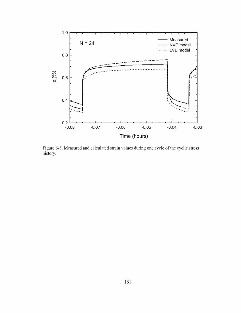
161

Time (hours)

-0.08 -0.07 -0.06 -0.05 -0.04 -0.03

ε (%

)

0.2

0.4

0.6

0.8

1.0

MeasuredNVE modelLVE model

N = 24

Figure 6-8. Measured and calculated strain values during one cycle of the cyclic stress history.

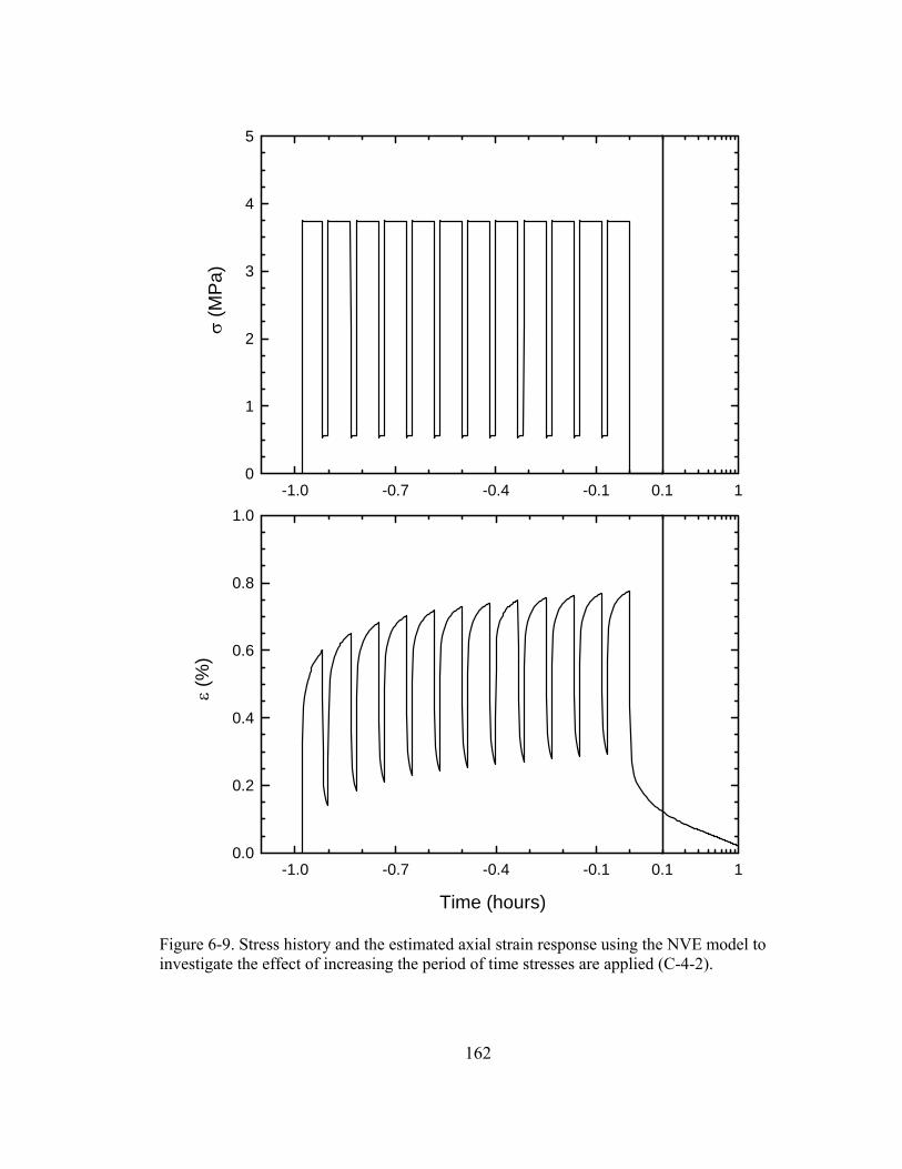
162

0.1 1-1.0 -0.7 -0.4 -0.1

σ (M

Pa)

0

1

2

3

4

5

0.1 1

Time (hours)

-1.0 -0.7 -0.4 -0.1

ε (%

)

0.0

0.2

0.4

0.6

0.8

1.0

Figure 6-9. Stress history and the estimated axial strain response using the NVE model to investigate the effect of increasing the period of time stresses are applied (C-4-2).

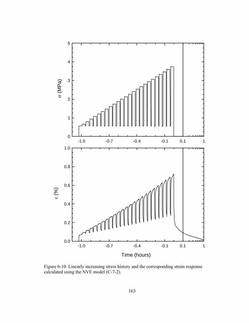
163

0.1 1-1.0 -0.7 -0.4 -0.1

σ (M

Pa)

0

1

2

3

4

5

0.1 1

Time (hours)

-1.0 -0.7 -0.4 -0.1

ε (%

)

0.0

0.2

0.4

0.6

0.8

1.0

Figure 6-10. Linearly increasing stress history and the corresponding strain response calculated using the NVE model (C-7-2).

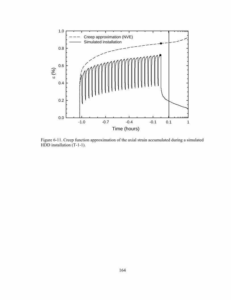
164

0.1 1

Time (hours)-1.0 -0.7 -0.4 -0.1

ε (%

)

0.0

0.2

0.4

0.6

0.8

1.0Creep approximation (NVE)Simulated installation

Figure 6-11. Creep function approximation of the axial strain accumulated during a simulated HDD installation (T-1-1).

165

Chapter 7

General discussion

7.1 Ground displacements and PVC water pipe response during pipe bursting

Detailed discussions of ground displacements during pipe bursting and the response of a PVC

water pipe to these displacements were given in Chapters 2 and 3. A synthesis of the results

and a general discussion on the implication of this work on pipe bursting operations are

presented here.

7.1.1 Ground displacements from a large-scale pipe bursting experiment in well-

graded sand

During pipe replacement by bursting, the expander will enlarge the soil cavity because the

diameter of the expander is larger than that of the existing pipe. In Chapter 2, a new

unreinforced concrete pipe, buried 1.39 m below the ground surface and having an inside

diameter of 150 mm, was burst using a 200 mm diameter expander in a well-graded sand and

gravel soil. For this degree of expansion, the component of the measured pulling force

required to expand the soil cavity was deemed to be approximately 100 – 130 kN, while 20 –

50 kN was attributed to the breaking of the existing concrete pipe. These pulling force

measurements were obtained by replacing a new unreinforced concrete pipe. If a deteriorated

unreinforced concrete pipe was replaced as opposed to a new pipe, the magnitude of pulling

force attributed to breaking the pipe would decrease since the pipe’s strength may be

reduced. During some pipe bursting installations, substantial pulling forces are required,

hence, pipe bursting equipment (e.g. rig, pull rods, expander) should be selected to ensure the

pulling force does not exceed the load capacity of the equipment used.

166

The maximum vertical surface displacement measured at the ground surface was 6

mm, while the distribution of vertical surface displacements extended no more than 2 m on

either side of the centreline. In addition to these vertical surface displacements, pipe bursting

induced transverse and axial surface displacements. The transverse surface displacements

generated a zone of tension above the existing pipe, as the ground surface was displaced

away from the centerline of the existing pipe. Acting within the zone of tension were tensile

strains which lead to the formation of tension cracks. It is uncertain whether the observed

cracking would have developed if an overlying pavement layer was present on the ground

surface, and it is difficult to assess the likelihood of damage to the pavement.

7.1.2 Response of a PVC water pipe when transverse to the replacement of an

underlying pipe by pipe bursting

In response to the ground deformations reported in Chapter 2, the maximum longitudinal

strain measured in the transverse PVC water pipe was 0.1%, corresponding to a peak vertical

displacement of 5 mm. When the expander was directly beneath the PVC pipe, the pipe’s

vertical diameter decreased by approximately 0.5%, which is much less than conventional

ring deflection limits for PVC, and when the expander progressed further past the PVC pipe,

these values decreased. This suggests that pipe bursting did not negatively impact the

particular PVC pipe tested.

Generally, ground deformations associated with pipe bursting are expected to be

greatest in the vicinity of the expanded cavity, and than attenuate outwards. However, the

vertical displacements measured at the ground surface, during the particular experiment

presented in Chapter 3, were greater than those of the PVC pipe. Since the flexural stiffness

of the PVC pipe was larger than the soil it replaces, it appears that the PVC pipe stiffens the

soil in its vicinity. However, there is no discernable stiffening of the soil by the PVC pipe

167

based on the measured surface response, suggesting that the soil restraint is restricted to the

zone immediately around the PVC pipe.

A simplified design equation based on beam theory was shown to provide a range of

calculated longitudinal strain values that was consistent with the strain measured in the PVC

pipe. Once more is learnt about the relationship between transverse utility displacements and

surface displacements for varying pipe bursting geometries and soil materials, this simplified

design equation might form the basis of a useful procedure for calculating the maximum

longitudinal strain.

The experimental data presented in Chapters 2 and 3 improves the understanding of

the mechanisms of ground disturbance, and the influence on an overlying transverse PVC

water pipe. The results reported could be used to evaluate the effectiveness of current

numerical models or for the calibration of models developed in the future.

7.2 HDPE pipe response during horizontal directional drilling

Detailed discussions of the stress-strain response of HDPE pipe during and after an HDD

installation were given in Chapters 4 to 6. A synthesis of the results and a general discussion

of the implications of this work on horizontal directional drilling operations are presented

here.

7.2.1 Axial stress-strain response of HDPE from whole pipes and coupons

To investigate the stress-strain response of HDPE pipes during and after a simulated HDD

installation, isolated whole pipe samples were tested rather than coupons trimmed from a

pipe wall. The merit of testing whole pipe samples as opposed to coupons was examined in

Chapter 4 by comparing results from stress relaxation and creep tests performed on whole

pipe samples against identical tests performed on coupons. These results suggested that the

168

coupons exhibited a higher modulus than the pipe samples. The cause for this apparent

increase in modulus that occurs in HDPE when a coupon is trimmed from a pipe wall is

unclear; however, it may be attributed to release of the residual stresses generated during the

extrusion process used to manufacture the pipes. In addition, a tension test performed on a

coupon will give the tensile properties only at a specific location on the pipe circumference,

whereas tension testing of the whole pipe sample will give the average tensile properties over

the entire pipe barrel. When the variation in the tensile properties around the circumference

of a pipe was investigated, it was found that all the tensile properties varied around the

circumference; however, only the secant modulus from 2% to 2.5% varied in a statistically

significant way.

Under most circumstances, the benefit of testing whole pipe samples as opposed to

testing coupons trimmed from a pipe wall is overshadowed by the relative ease in which

experiments on coupons can be conducted compared to the complexities that arise when

testing a whole pipe sample; however, because the whole pipe barrel is subjected to axial

tensile stresses and strains during an actual HDD installation, the whole pipe was tested in

this project to investigate HDPE response during HDD.

7.2.2 Stress-strain measurements for HDPE pipe during and after simulated

installation by HDD

The results of Chapter 5 showed the stress-strain response of a pipe sample during the three

stages of HDD simulated in the laboratory: installation, recovery, and restraint. During

installation, a pulled-in-place pipe must be able to resist the tensile axial stress imposed to

pull the pipe through the borehole. ASTM F1804 stipulates that the short-term tensile axial

stress imposed should not exceed the allowable tensile load to avoid imposing stresses

beyond yield.

169

After installation, the long-term performance of a pulled-in-place HDPE pipe

depends on the pipe’s ability to resist the axial tensile stress redeveloped in the pipe after it is

restrained, in addition to hoop stresses generated from external or internal loading (e.g.

overburden material and, in the case of pressure pipe, the internal working pressure).

For the conditions simulated in the laboratory, the tensile axial stress redeveloped in

the pipe did not exceed long-term tensile stresses that would lead to stress conditions

conducive to slow crack growth, when circumferential stress limits are adopted as the axial

stress limits. Even when short-term performance limits were exceeded during installation and

allowed to recover for at least 1 hour, the tensile stresses that develop after 100 hours were

below the long-term performance limits. However, if the redeveloped stresses were deemed

to be excessive, the length of the recovery period could be extended to minimize the

magnitude of the redeveloped stresses.

7.2.3 Effectiveness of viscoelastic models for prediction of tensile axial strains during

cyclic loading of HDPE

In Chapter 6, existing linear and nonlinear viscoelastic models were shown to provide

reasonable estimates of the maximum strain levels during installation. Viscoelastic models

were used to predict the tensile axial strain during cyclic loading of HDPE because they

feature the two most important characteristics of the cyclic response of HDPE: strain

accumulation under constant stress, and strain recovery following unloading. More

specifically, the viscoelastic models of Moore and Hu (1996) and Zhang and Moore (1997a)

were used as opposed to other available viscoelastic models because parameters for both of

these models were available for the same HDPE pipe material tested in the laboratory.

In order to estimate the axial strain accumulated during an HDD installation, it was

shown that conventional creep curves can be used provided the maximum pulling force is

170

known. For instance, for a given HDD installation, the maximum pulling force can be

calculated using equations suggested by Baumert and Allouche (2002) and using the

nonlinear viscoelastic model, this pulling force can be constantly imposed to generate a pure

creep curve.

7.3 References

ASTM F 1804-08. Standard Practice for Determining Allowable Tensile Load for

Polyethylene (PE) Gas Pipe During Pull-In Installation. ASTM International, West

Conshohocken, PA.

Baumert, M. E. and Allouche, E. N. 2002, ‘Methods for estimating pipe pullback loads for

horizontal directional drilling crossings’, Journal of Infrastructure Systems, ASCE, 8(1):

12-19.

Moore, I.D. and Hu, F., 1996. Linear viscoelastic modeling of profiled high density

polyethylene pipe. Canadian Journal of Civil Engineering, 23(2): 395-407

Zhang, C., and Moore, I.D. 1997a. Nonlinear mechanical response of high density

polyethylene. Part I: Experimental investigation and model evaluation. Polymer

Engineering and Science, 37(2): 404-413

171

Chapter 8

Conclusions and recommendations

8.1 Ground displacements and PVC water pipe response during pipe bursting

The ground displacements associated with pipe bursting in well-graded sand and gravel soil

and the effect these ground displacements had on an adjacent PVC water pipe were

investigated. A large-scale static pipe bursting experiment was conducted in an 8-m-long, 8-

m-wide, and 3-m-deep test pit with an unreinforced concrete pipe, buried 1.39 m below the

ground surface, being replaced by an HDPE pipe. A PVC pipe, instrumented with strain

gages, was buried 0.45 m above and transverse to the unreinforced concrete pipe. The pulling

force and the three-dimensional nature of the ground displacements associated with pipe

bursting were quantified. The response of the PVC water pipe was also evaluated in terms of

longitudinal and circumferential strain and the corresponding pipe deflections.

8.1.1 Ground displacements from a large-scale pipe bursting experiment in well-

graded sand

In Chapter 2, the pulling force and ground displacements associated with pipe bursting were

quantified. For the specific conditions tested, the average pulling force required was 149 kN,

and the maximum pulling force was 209 kN. This included the force required to break the

existing pipe, expand the soil cavity and move the expander forward, and overcome friction

on the new HDPE pipe. In terms of surface displacements, a point on the ground surface

moved vertically upwards, transversely outwards, and axially forwards when the expander

approached. The permanent surface displacement was vertically upwards, transversely

outwards, and axially backwards from its original position. The maximum vertical surface

displacement measured during the test was 6 mm. A zone of tension was created when the

172

ground surface displaced horizontally away from the centerline of the existing pipe. The

corresponding transverse tensile strains cracked the sand and gravel at the ground surface

close to points directly above the pipe centreline.

8.1.2 Response of a PVC water pipe when transverse to the replacement of an

underlying pipe by pipe bursting

The nature of adjacent pipe bending that occurs as a result of the ground movements induced

by pipe bursting operations was quantified in Chapter 3. In response to the ground

deformations associated with replacement of an unreinforced concrete pipe with an HDPE

pipe, the maximum longitudinal strain measured in the PVC water pipe was 0.1%,

corresponding to a peak vertical displacement of 5 mm. A simplified design equation based

on beam bending theory, was found to provide a range of longitudinal strain values that

included the strains measured in the PVC pipe. The permanent displacement of both the

ground surface and the PVC pipe was upwards and backwards; however, the magnitude of

these displacements was slightly larger for the ground surface than for the pipe. This was

attributed to the PVC pipe having higher flexural stiffness than the soil it replaces, although

there was no discernable stiffening of the soil by the PVC pipe based on the measured surface

response, suggesting that the soil restraint is restricted to the zone immediately around the

PVC pipe. The PVC pipe’s vertical diameter decreased by 0.5% when the expander was

directly beneath it, much less than conventional ring deflection limits for PVC, suggesting

that pipe bursting did not negatively impact the particular PVC pipe tested.

8.2 HDPE pipe response during horizontal directional drilling

The stress-strain response of pulled-in-place HDPE pipe was quantified during and after

simulated HDD installations. Prior to examining the complex behaviour of pulled-in-place

pipe, the time-dependant nature of HDPE was quantified by performing a series of creep and

173

stress relaxation tests using two types of isolated whole pipe samples and coupons trimmed

around the circumference of a pipe barrel. Based on these results, the merit of testing whole

pipe samples as opposed to testing coupons was examined. Further, whole pipe samples were

tested to quantify the stress-strain response of HDPE pipe during a series of simulated HDD

installations and the subsequent strain recovery and pipe restraint periods. The ability of two

existing viscoelastic models to calculate the cyclic strain history of HDPE pipe during a

simulated HDD installation was also evaluated.

8.2.1 Axial stress-strain response of HDPE from whole pipes and coupons

Results from identical stress relaxation and creep tests performed on whole pipe samples and

coupons presented in Chapter 4 suggest that the coupons exhibited a higher modulus than the

pipe samples. The apparent increase in modulus when specimens are trimmed from a pipe

wall may be attributed to the release of residual stresses. Under most circumstances, the

benefits of testing whole pipe samples are overshadowed by the relative ease in which

experiments on coupons can be conducted compared to the complexities that arise when

testing a whole pipe sample; however, because the whole pipe barrel is subjected to axial

tensile stresses and strains during an actual HDD installation, the whole pipe was tested in

this study of HDPE response during HDD.

8.2.2 Stress-strain measurements for HDPE pipe during and after simulated

installation by HDD

In Chapter 5, the impact the tensile axial stresses and strains, induced during and after a

simulated HDD installation, had on an HDPE pipe was evaluated. Generally, axial strains

progressively accumulated when an HDPE pipe sample was subjected to the cyclic stress

history used to simulate an HDD installation. The magnitude of these strains depended on the

pulling force, length of pipe installed, and drilling rod length. For the specific conditions

174

examined, the tensile axial stresses redeveloped in the pipe samples, once restrained, were

not large enough to lead to long-term stress conditions conducive to slow crack growth. In

fact, the available data suggests that limiting the installation force to values stipulated by

ASTM F1804 and allowing a minimum of 24 hours of recovery time is sufficient to ensure

adequate long-term pipe performance, provided the pipe is not excessively scratched during

installation.

8.2.3 Effectiveness of viscoelastic models for prediction of tensile axial strains during

cyclic loading of HDPE

In Chapter 6, the ability of existing linear and nonlinear viscoelastic models (Moore and Hu,

1996; Zhang and Moore, 1997) to serve as predictive design tools for estimating the cyclic

strain history of HDPE pipe during an HDD installation was evaluated. When compared

against results from the experiments conducted on pipe samples in Chapter 5, the linear and

nonlinear viscoelastic models provide reasonable estimates of the maximum strain levels

during installation; however, maximum strains were underestimated by the linear viscoelastic

model and overestimated by the nonlinear viscoelastic model. During periods of strain

reversal, both models overestimated the amount of axial strain recovery. Using the nonlinear

viscoelastic model to study axial pipe response under pure creep provided a conservative

estimate of the maximum axial strain accumulated during an HDD installation, provided the

maximum pulling force is known.

8.3 Applicability, limitations, and future work

8.3.1 Ground displacements and PVC water pipe response during pipe bursting

The results presented in Chapters 2 and 3 were obtained by performing a single large-scale

pipe bursting experiment and are applicable only to the specific materials and conditions

tested. Caution should be exercised when using these results to predict the behaviour of

175

different soil types, pipe materials, and pipe bursting geometries. However, the experiment

offers data that improves the understanding of the mechanisms of ground disturbance, and

provides unique experimental data for calibration of numerical models. In fact, the data

presented in chapters 2 and 3 is being used to develop a three-dimensional finite element

model capable of calculating ground response to pipe bursting. Although, to fully develop

this three-dimensional model, future research is required to fully understand the nature of

ground displacements and PVC water pipe response associated with pipe bursting in different

soil materials and pipe bursting geometries.

This data is of particular interest because it can be used to further develop the

simplified design equation presented in Chapter 3 by relating transverse utility displacements

to surface displacements. In addition, further work is required to determine if the transverse

tensile strains acting on the ground surface in Chapter 2 can develop if an overlying

pavement layer is present, and the likelihood of damage to the pavement. This has also been

identified as an area requiring further research by Chapman et al. (2007).

8.3.2 HDPE pipe response during horizontal directional drilling

The results presented in Chapters 4 to 6 apply only to the specific pipe material and

conditions tested. Caution should be exercised when applying these results to different pipe

materials, temperatures, and loading conditions. The stresses and strains reported were

obtained using one particular set of idealized stress histories; however, stress histories during

actual HDD installations are more complex and variable suggesting the maximum axial strain

accumulated is specific to a particular installation.

176

Further research is required to fully understand the stress-strain response of pulled-in-

place PVC pipe under the same conditions presented in this thesis, since PVC pipes are

becoming more widely used for pulled-in-place pipe applications.

8.4 References

ASTM F 1804-08. Standard Practice for Determining Allowable Tensile Load for

Polyethylene (PE) Gas Pipe During Pull-In Installation. ASTM International, West

Conshohocken, PA.

Chapman, D.N., Ng, P.C.F. and Karri, R. 2007. Research needs for on-line pipeline

replacement techniques. Tunnelling and Underground Space Technology, 22(5), 503-

514.

Moore, I.D. and Hu, F., 1996. Linear viscoelastic modeling of profiled high density

polyethylene pipe. Canadian Journal of Civil Engineering, 23(2): 395-407

Zhang, C. and Moore, I.D. 1997. Nonlinear mechanical response of high density

polyethylene. Part II: Uniaxial constitutive modeling. Polymer Engineering and Science,

37(2): 414-420

177

Appendix A

Procedure used to determine the accuracy of displacement

measurements obtained from digital cameras

The three-dimensional surface displacements, reported in chapters 2 and 3, were measured

using 349 targets placed on the ground surface. Two digital cameras were used to track the

movement of each target, in terms of pixels, during the replacement of the unreinforced

concrete pipe. Both of the cameras tracked vertical surface movements, however, the axial

camera, located at x = 4 m and z = 4 m, tracked axial movements, while the transverse

camera, located at x = 0 and z = -8 m, tracked transverse movements. The field of views for

these cameras are given in Figures A-1a and A-1b respectively. Surface displacements were

calculated by analyzing the images obtained from these cameras using the image-based

deformation software, geoPIV (White et al., 2003).

To determine the accuracy of the displacement measurements obtained from the

digital cameras, images of the ground surface were analyzed over a period of zero

displacement. The axial and vertical movement (in pixels) obtained from the axial camera are

given in Figures A-2 and A-3 respectively. Here, the average movement of 15 targets located

along x = 0 (as shown in Figure A-1a), is plotted over a 4.5 hour period. Axial and vertical

movements obtained using the axial camera were less than ± 0.1 pixels. The transverse and

vertical movement (in pixels) obtained from the transverse camera are given in Figures A-4

and X-5 respectively. Here, the average movement of 25 targets located along z = 4.92 m (as

shown in Figure A-1b), is plotted over a 4.5 hour period. Transverse and vertical movements

obtained using the transverse camera were typically less than ± 0.2 pixels. The axial camera’s

resolution was better than that of the transverse camera, since the transverse camera was

178

located approximately 13 m from z = 4.92 m, while the axial camera was located only 4 m

from x = 0.

Displacements (in mm) were calculated from pixels by applying a pixel conversion

factor. Tables X-1 and X-2 gives the pixel conversion factors used for the axial and

transverse cameras respectively. From Table X-1, the conversion factor varies from 0.4

mm/pixel to 1.4 mm/pixel, and increases further away from the camera. For the transverse

camera, the conversion factor increases from 0.9 mm/pixel to 1.6 mm/pixel (Table X-2).

Using the resolution determined from Figure A-2 to A-5 and the pixel conversion

factors given in Tables X-1 and X-2, the accuracy of the axial camera ranged from ± 0.04

mm to ± 0.14 mm and the accuracy of the transverse camera ranged from ± 0.18 mm to ±

0.32 mm. The accuracy depends on the location of the target relative to the camera tracking

it; however, during the experiment reported in chapters 2 and 3, the accuracy did not exceed

± 0.3 mm.

References

White, D.J., Take, W.A. and Bolton, M.D. 2003. Soil deformation measurement using

particle image velocimetry (PIV) and photogrammetry. Geotechnique 53 (7):619-631.

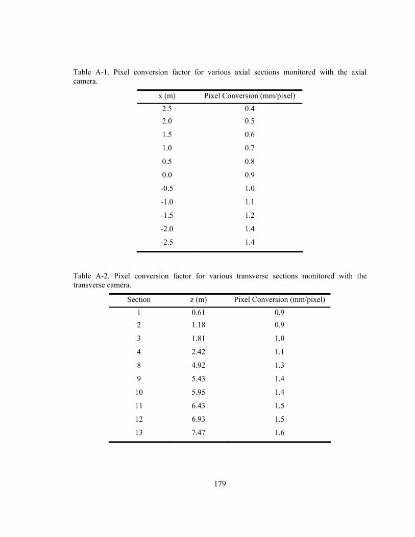
179

Table A-1. Pixel conversion factor for various axial sections monitored with the axial camera.

x (m) Pixel Conversion (mm/pixel)

2.5 0.4 2.0 0.5

1.5 0.6

1.0 0.7

0.5 0.8

0.0 0.9

-0.5 1.0

-1.0 1.1

-1.5 1.2

-2.0 1.4

-2.5 1.4

Table A-2. Pixel conversion factor for various transverse sections monitored with the transverse camera.

Section z (m) Pixel Conversion (mm/pixel)

1 0.61 0.9 2 1.18 0.9

3 1.81 1.0

4 2.42 1.1

8 4.92 1.3

9 5.43 1.4

10 5.95 1.4

11 6.43 1.5

12 6.93 1.5

13 7.47 1.6

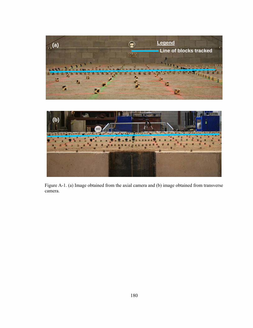
180

Figure A-1. (a) Image obtained from the axial camera and (b) image obtained from transverse camera.

(a)

(b)

Line of blocks tracked Legend

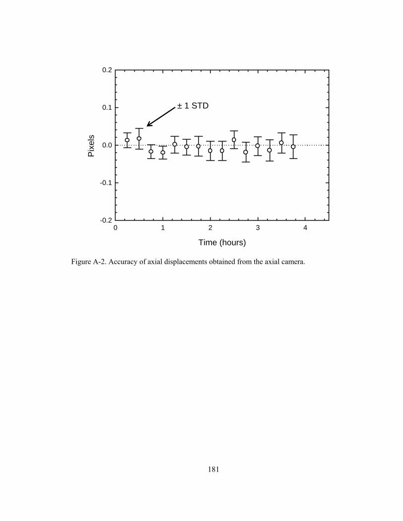
181

Time (hours)

0 1 2 3 4

Pix

els

-0.2

-0.1

0.0

0.1

0.2

Figure A-2. Accuracy of axial displacements obtained from the axial camera.

± 1 STD

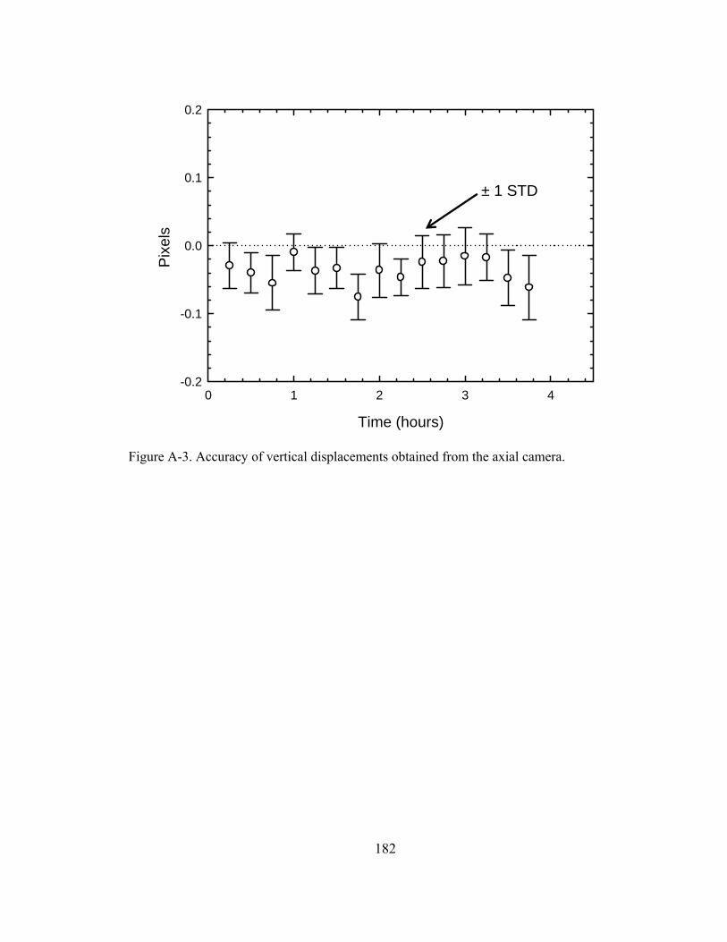
182

Time (hours)

0 1 2 3 4

Pix

els

-0.2

-0.1

0.0

0.1

0.2

Figure A-3. Accuracy of vertical displacements obtained from the axial camera.

± 1 STD

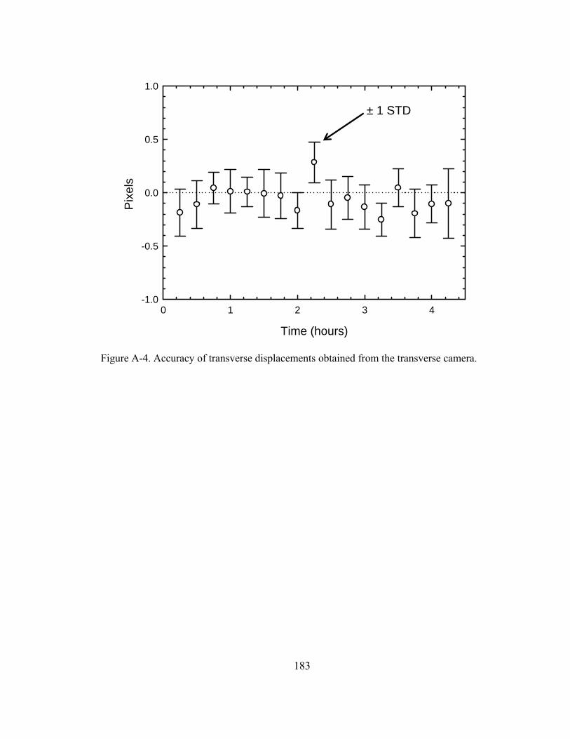
183

Time (hours)

0 1 2 3 4

Pix

els

-1.0

-0.5

0.0

0.5

1.0

Figure A-4. Accuracy of transverse displacements obtained from the transverse camera.

± 1 STD

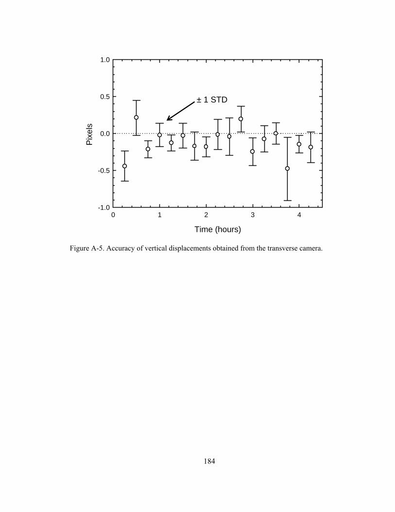
184

Time (hours)

0 1 2 3 4

Pix

els

-1.0

-0.5

0.0

0.5

1.0

Figure A-5. Accuracy of vertical displacements obtained from the transverse camera.

± 1 STD

185

Appendix B

Surface scratches on an HDPE pipe installed by pipe bursting

B.1 Introduction

During a pulled-in-place installation, either by horizontal directional drilling (HDD) or pipe

bursting, the new high density polyethylene (HDPE) pipe being pulled into place may be

scratched, thereby decreasing the wall thickness. For pressure pipe applications, the presence

of these surface scratches, may initiate slowly growing cracks in the semicrystalline structure

of HDPE (Mruk, 1990). If these scratches are significant enough, the HDPE pipe may be

prone to failure at stresses less than the hydrostatic design basis (forecasted by plotting

circumferential stress versus time-to-failure for an unscratched pipe under constant internal

pressures and extrapolating to the 100,000 hour intercept in accordance with ASTM D2837).

During pipe bursting installations of pressure pipe, scratching of the new HDPE pipe is

typically offset by increasing the pipe’s long-term wall thickness requirement by 10%;

however, if surface scratching is deemed to be an issue, a sleeve pipe can be installed during

the bursting operation with the new HDPE pipe installed later within the sleeve (Simicevic

and Sterling, 2001).

The performance of scratched HDPE pipes was examined Zhou and Chang (2006).

To mimic installation scratches, 60° V-shaped notches were introduced along the longitudinal

axis of two types of HDPE pipe samples at depths of 5%, 10%, and 15% the minimum wall

thickness. Hydrostatic burst tests (ASTM D1598) were conducted at 90°C and 80°C on these

scratched pipe samples and compared against virgin (un-scratched) pipe samples. It was

found that, even though the failure times for the scratched pipe samples were generally less

than virgin pipe samples, the scratched pipe samples still met the minimum hydrostatic

186

design basis for the HDPE pipe tested. This suggests that the particular scratches introduced

did not jeopardize the long-term performance of the HDPE pipe samples tested.

During the large-scale pipe bursting experiment presented in Chapters 2 and 3, a new

8 m long HDPE pipe was installed in an unreinforced concrete pipe. The resulting scratches

incurred on the surface of the HDPE pipe, from interacting with the broken fragments of

unreinforced concrete pipe, are quantified here.

B.2 Experimental details

In Chapters 2 and 3, results from a large-scale static pipe bursting experiment conducted in

an 8-m-long, 8-m-wide, and 3-m-deep test pit with an unreinforced concrete pipe being

replaced by an HDPE pipe were reported. Once installed, the new HDPE replacement pipe,

having an outside diameter of 168 mm and an average wall thickness of 11 mm, was

exhumed to quantify the surface damage incurred. The location around the pipes

circumference and length of the most significant scratches were measured using a standard

tape measure. The width and depth of the scratches were measured using a line laser accurate

to 0.04 mm.

B.3 Results

Among many minor scratches and abrasions, the pipe incurred two significant scratches to its

surface during installation (denoted as scratch 1 and 2). The location and length of these

scratches are given along the length of the pipe in Figure B-1. Here, the crown and invert of

the pipe, once it was installed, was located at 0° and ±180° respectively. The pipe section

located at z = 8 m was pulled through the entire 8 m length of the unreinforced concrete pipe

(conversely, the pipe section located at z = 2 m was pulled through 2 m of the concrete pipe).

The results in Figure B-1 show that scratch 1 was approximately 4.5 m in length and was

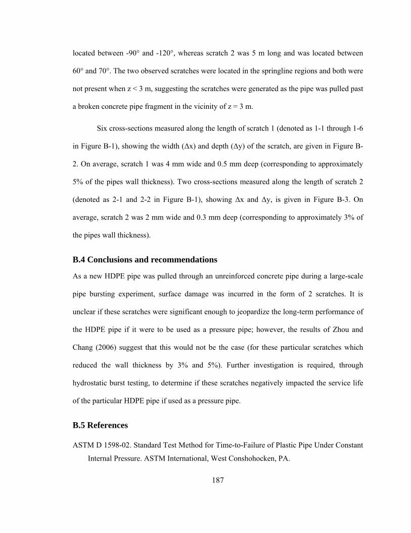
187

located between -90° and -120°, whereas scratch 2 was 5 m long and was located between

60° and 70°. The two observed scratches were located in the springline regions and both were

not present when z < 3 m, suggesting the scratches were generated as the pipe was pulled past

a broken concrete pipe fragment in the vicinity of z = 3 m.

Six cross-sections measured along the length of scratch 1 (denoted as 1-1 through 1-6

in Figure B-1), showing the width (Δx) and depth (Δy) of the scratch, are given in Figure B-

2. On average, scratch 1 was 4 mm wide and 0.5 mm deep (corresponding to approximately

5% of the pipes wall thickness). Two cross-sections measured along the length of scratch 2

(denoted as 2-1 and 2-2 in Figure B-1), showing Δx and Δy, is given in Figure B-3. On

average, scratch 2 was 2 mm wide and 0.3 mm deep (corresponding to approximately 3% of

the pipes wall thickness).

B.4 Conclusions and recommendations

As a new HDPE pipe was pulled through an unreinforced concrete pipe during a large-scale

pipe bursting experiment, surface damage was incurred in the form of 2 scratches. It is

unclear if these scratches were significant enough to jeopardize the long-term performance of

the HDPE pipe if it were to be used as a pressure pipe; however, the results of Zhou and

Chang (2006) suggest that this would not be the case (for these particular scratches which

reduced the wall thickness by 3% and 5%). Further investigation is required, through

hydrostatic burst testing, to determine if these scratches negatively impacted the service life

of the particular HDPE pipe if used as a pressure pipe.

B.5 References

ASTM D 1598-02. Standard Test Method for Time-to-Failure of Plastic Pipe Under Constant

Internal Pressure. ASTM International, West Conshohocken, PA.

188

ASTM D 2837-04. Standard Test Method for Obtaining Hydrostatic Design Basis for

Thermoplastic Pipe Materials or Pressure Design Basis for Thermoplastic Pipe Products.

ASTM International, West Conshohocken, PA.

Mruk, S.A. 1990. The durability of polyethylene piping, Buried Plastic Pipe Technology.

ASTM STP 1093, G.S. Buczala and M.J. Cassady (Eds.) ASCE, pp 21-39

Simicevic, J., and Sterling, R.L. 2001. Guidelines for pipe bursting. TTC technical report

#2001.02, U.S. Army Corps of Engineers.

Zhou, Z.J., and Chang, D. 2006. Performance of Scratched HDPE Pressure Pipe. Plastic

Pipes XIII Conference Proceedings. Washington, D.C., October 2-5, 2006.

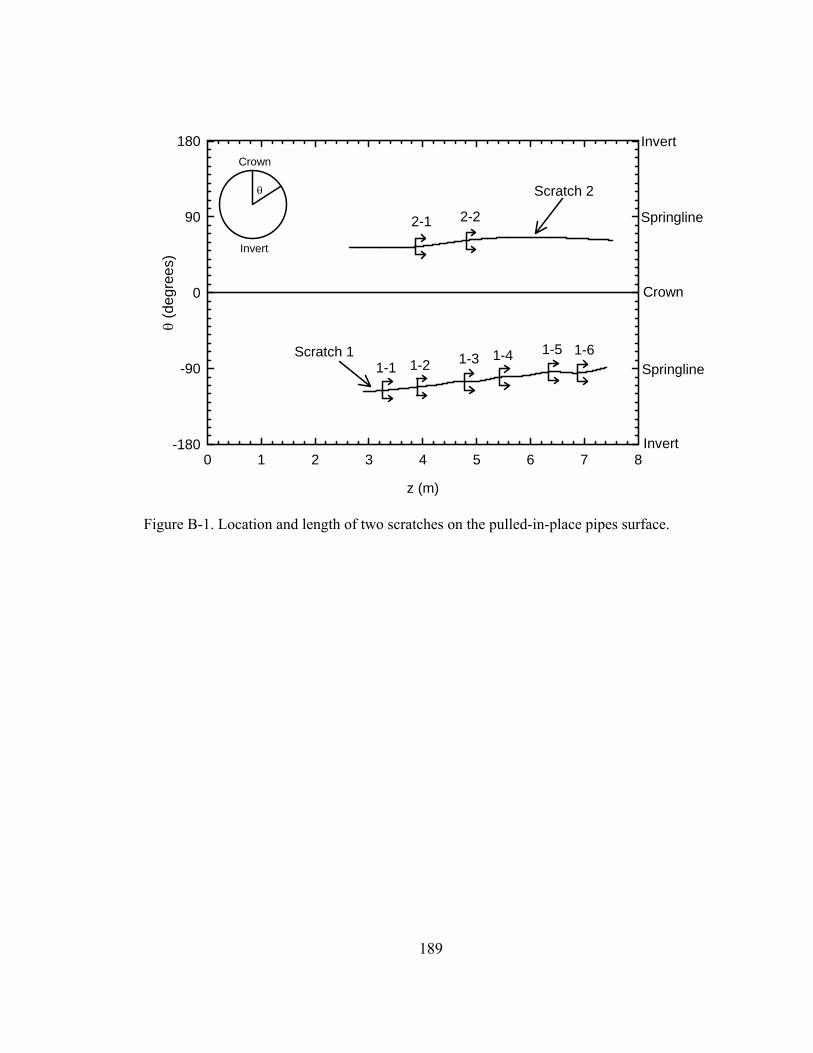
189

z (m)

0 1 2 3 4 5 6 7 8

θ (d

egre

es)

-180

-90

0

90

180

Crown

Invert

Invert

Springline

Springline

Invert

Crown

θ

1-1 1-2 1-3 1-4 1-5 1-6

2-1 2-2

Scratch 1

Scratch 2

Figure B-1. Location and length of two scratches on the pulled-in-place pipes surface.

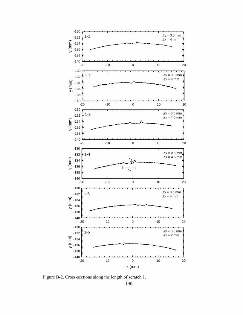
190

20100-10-20

y (m

m)

-140

-138

-136

-134

-132

-130

-20 -10 0 10 20y

(mm

)

-140

-138

-136

-134

-132

-130

20100-10-20

y (m

m)

-140

-138

-136

-134

-132

-130

-20 -10 0 10 20

y (m

m)

-140

-138

-136

-134

-132

-130

-20 -10 0 10 20

y (m

m)

-140

-138

-136

-134

-132

-130

x (mm)20100-10-20

y (m

m)

-140

-138

-136

-134

-132

-130

1-1

1-2

1-3

1-4

1-5

1-6

Δx

Δy

Δy = 0.5 mmΔx = 4 mm

Δy = 0.5 mmΔx = 4 mm

Δy = 0.6 mmΔx = 4.5 mm

Δy = 0.5 mmΔx = 4.5 mm

Δy = 0.5 mmΔx = 4 mm

Δy = 0.3 mmΔx = 2 mm

Figure B-2. Cross-sections along the length of scratch 1.

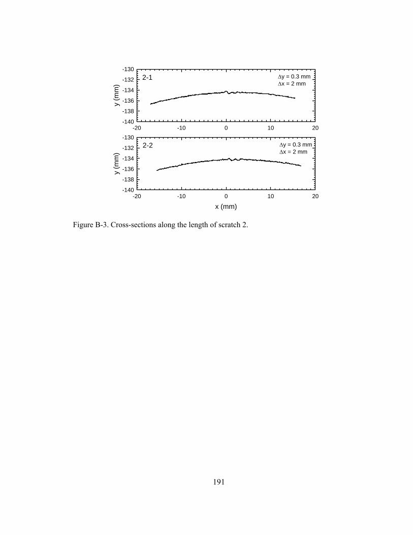
191

-20 -10 0 10 20

y (m

m)

-140

-138

-136

-134

-132

-130

x (mm)20100-10-20

y (m

m)

-140

-138

-136

-134

-132

-130

2-1

2-2

Δy = 0.3 mmΔx = 2 mm

Δy = 0.3 mmΔx = 2 mm

Figure B-3. Cross-sections along the length of scratch 2.

192

Appendix C

Procedure used for determining horizontal ground surface strain

from measurements of horizontal surface displacements

The horizontal strain reported in Chapter 2 was approximated by:

xu

xu

xx ΔΔ

=∂∂

=ε [C-1]

where: Δu is the incremental horizontal surface displacement and Δx is the incremental

transverse distance. The horizontal surface displacements (u) reported in Chapter 2 at z =

6.43 m when ZB = 6.93 m are given in Figure C-1. Here, a spline was drawn to closely fit the

measured data points. This method was selected over conventional curve fitting (i.e.

calculating strain by differentiating the equation of that curve with respect to x), because it

was difficult to provide a reasonable fit for the measured data points. Figure C-2a shows the

fitted line from Figure C-1 divided into multiple line segments from x = -1.52 m to -1.5 m.

Determining the slope of each of these individual line segments corresponded to the

horizontal strain at that particular location (Figure C-2b). The distribution of horizontal

strains acting on the surface was calculated using this procedure for various locations along x

(Figure C-3).

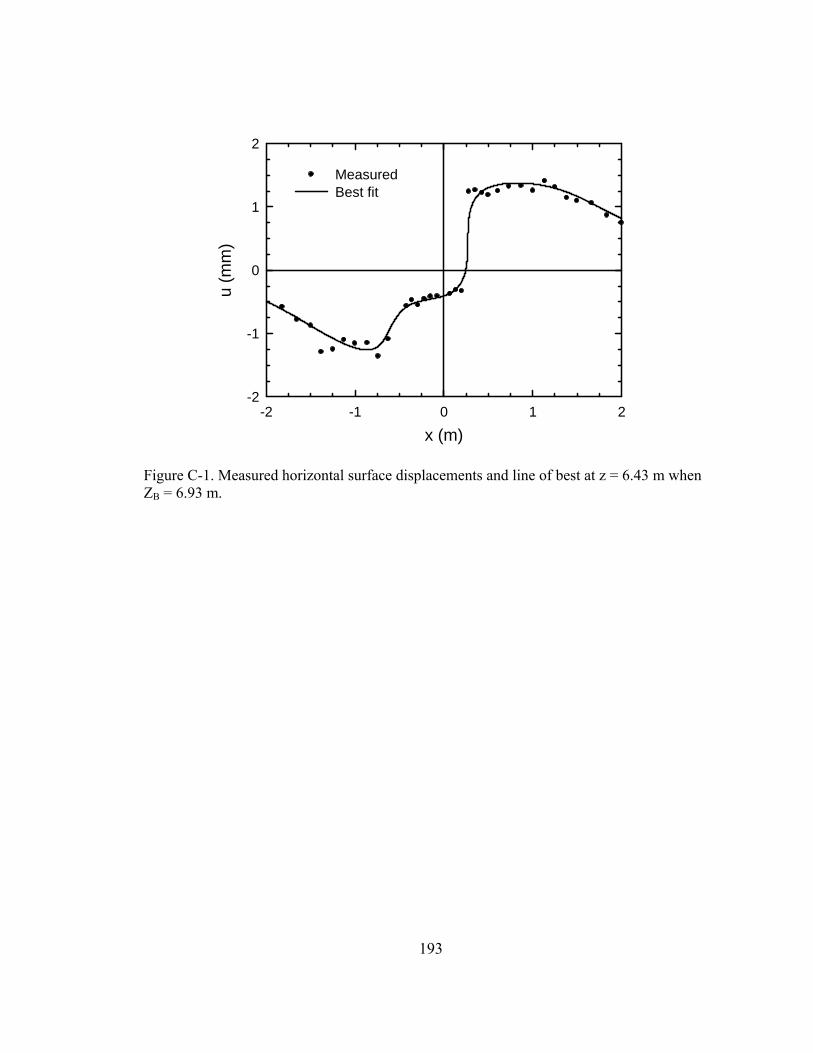
193

x (m)-2 -1 0 1 2

u (m

m)

-2

-1

0

1

2

MeasuredBest fit

Figure C-1. Measured horizontal surface displacements and line of best at z = 6.43 m when ZB = 6.93 m.

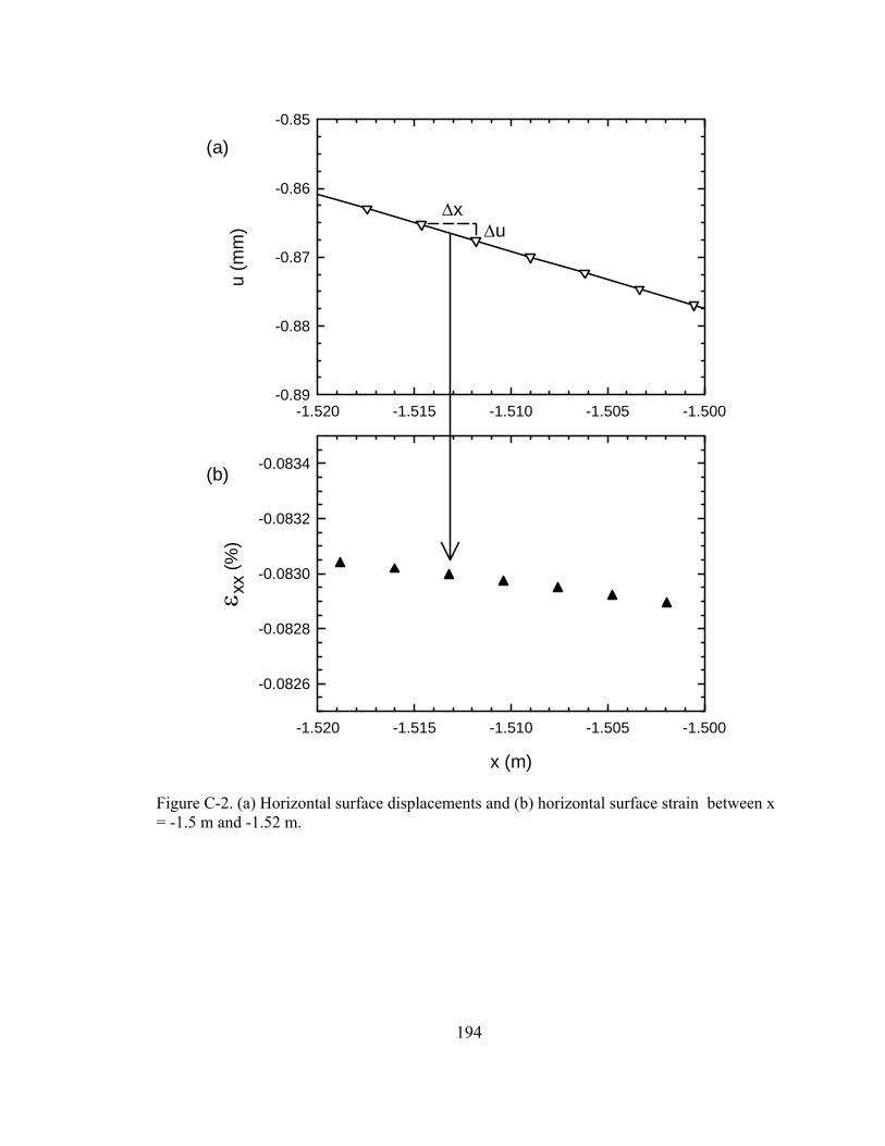
194

-1.520 -1.515 -1.510 -1.505 -1.500

u (m

m)

-0.89

-0.88

-0.87

-0.86

-0.85

ΔxΔu

x (m)

-1.520 -1.515 -1.510 -1.505 -1.500

ε xx

(%)

-0.0834

-0.0832

-0.0830

-0.0828

-0.0826

(a)

(b)

Figure C-2. (a) Horizontal surface displacements and (b) horizontal surface strain between x = -1.5 m and -1.52 m.

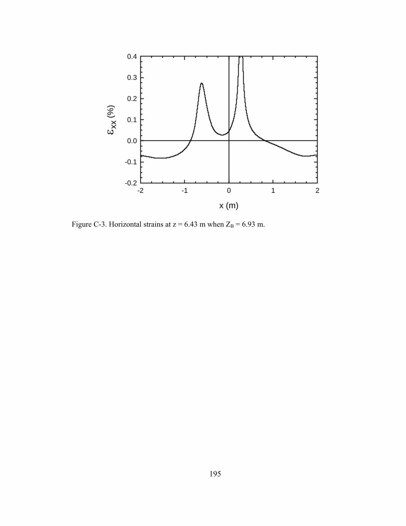
195

x (m)

-2 -1 0 1 2

ε xx

(%)

-0.2

-0.1

0.0

0.1

0.2

0.3

0.4

Figure C-3. Horizontal strains at z = 6.43 m when ZB = 6.93 m.

196

Appendix D

Procedure used for determining the vertical displacement of the

PVC pipe from its curvature

The curvature (κ) of the PVC pipe reported in Chapter 3 when ZB = 5.43 m is given in Figure

D-1. Here, a spline was drawn to closely fit the calculated curvature values. This method was

selected because it was difficult to provide a reasonable fit for the calculated data points

using conventional curve fitting. To calculate the vertical displacement for the PVC pipe,

conventional thin beam theory was used such that:

2

2

=dx

vdκ [D-1]

Using this expression and integrating curvature twice, the distribution of vertical

displacement for the PVC pipe was calculated.

First, the curvature of the PVC was integrated by calculating the area under the line

of best fit, shown in Figure D-1. Figure D-2a shows the curvature of the PVC pipe over a

0.025 m interval and the method used to calculate the area under the curve (i.e. how the first

integral of curvature was evaluated), while Figure D-2b gives the sum of the areas of the

rectangles over that same interval. The distribution of the sum of the areas from x = -3 m to 3

m is shown in Figure D-3a. Integration constants were determined by assuming the sum of

the areas at x = 2.75 m and -2.75 m were zero, therefore the function is rotated about x = -

2.75 m until the sum of the areas at x = 2.75 m was zero (as shown in Figure D-3b).

Once the first integral of curvature was evaluated, the second integral was evaluated

using the same procedure to calculate vertical displacement (v) of the PVC pipe. As a result,

the area under the curve shown in Figure D-3b is given in Figure D-4a. By assuming the

197

displacements at the ends of the PVC pipe were zero, the function is rotated about x = -2.75

m until the displacement at x = 2.75 m was zero (as shown in Figure D-4b).

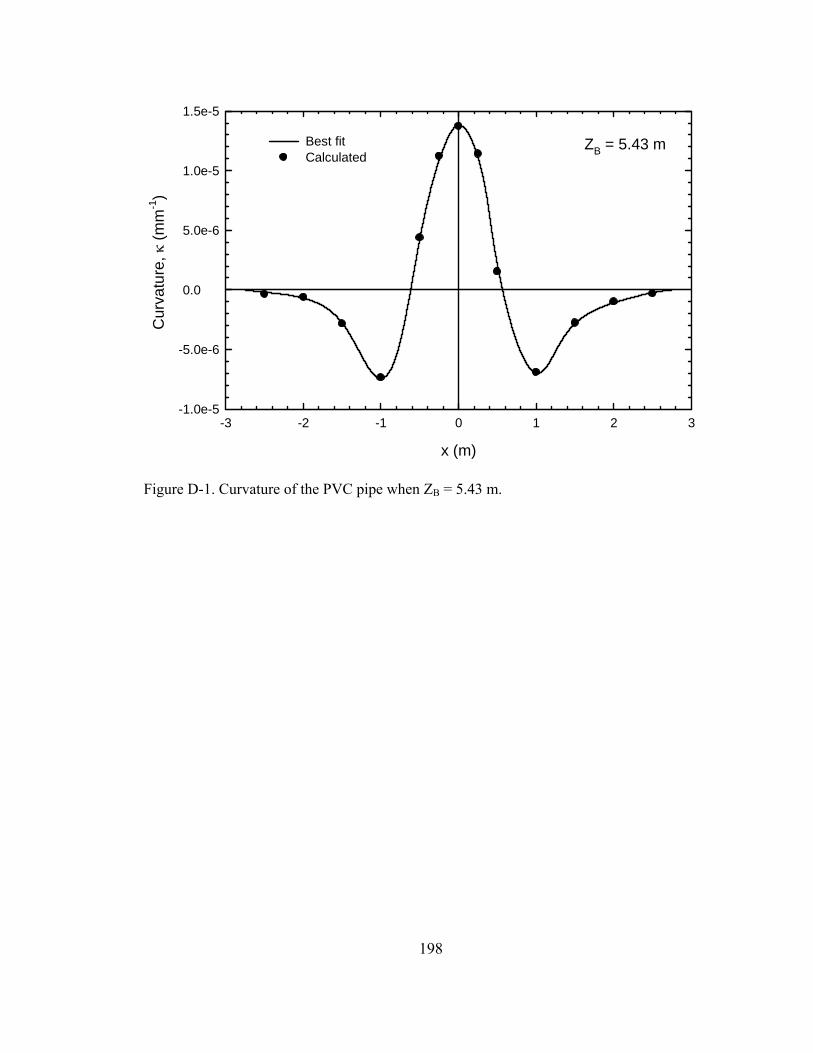
198

x (m)

-3 -2 -1 0 1 2 3

Cur

vatu

re, κ

(mm

-1)

-1.0e-5

-5.0e-6

0.0

5.0e-6

1.0e-5

1.5e-5

Best fitCalculated

ZB = 5.43 m

Figure D-1. Curvature of the PVC pipe when ZB = 5.43 m.

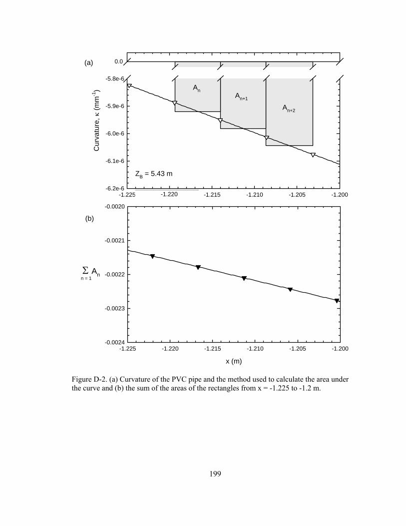
199

-1.225 -1.220 -1.215 -1.210 -1.205 -1.200

Cur

vatu

re, κ

(mm

-1)

-6.2e-6

-6.1e-6

-6.0e-6

-5.9e-6

-5.8e-6

0.0

x (m)

-1.225 -1.220 -1.215 -1.210 -1.205 -1.200-0.0024

-0.0023

-0.0022

-0.0021

-0.0020

ZB = 5.43 m

0.0

An+2

An+1

An

0.0

Σ Ann = 1

(a)

(b)

Figure D-2. (a) Curvature of the PVC pipe and the method used to calculate the area under the curve and (b) the sum of the areas of the rectangles from x = -1.225 to -1.2 m.

-1.220

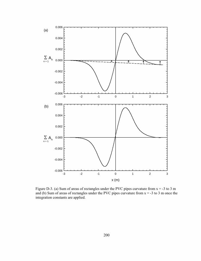
200

x (m)

-3 -2 -1 0 1 2 3-0.006

-0.004

-0.002

0.000

0.002

0.004

0.006

-3 -2 -1 0 1 2 3-0.006

-0.004

-0.002

0.000

0.002

0.004

0.006

Σ Ann = 1

Σ Ann = 1

(a)

(b)

Figure D-3. (a) Sum of areas of rectangles under the PVC pipes curvature from x = -3 to 3 m and (b) Sum of areas of rectangles under the PVC pipes curvature from x = -3 to 3 m once the integration constants are applied.

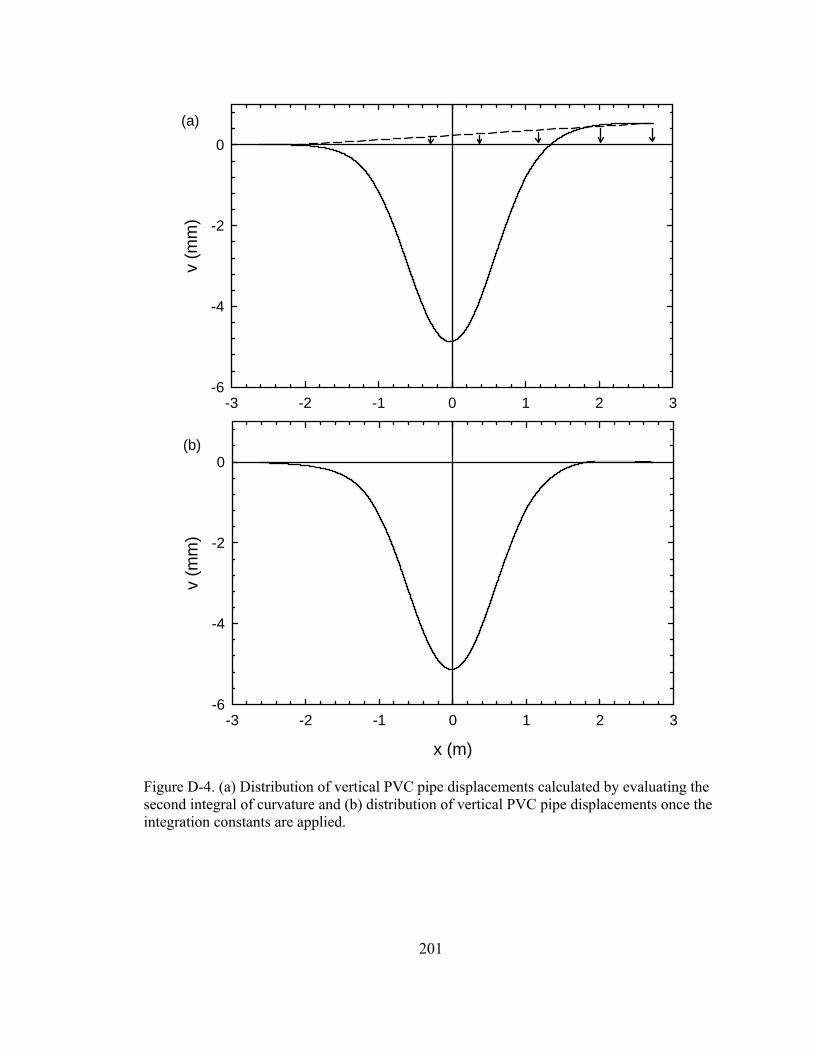
201

x (m)

-3 -2 -1 0 1 2 3

v (m

m)

-6

-4

-2

0

-3 -2 -1 0 1 2 3

v (m

m)

-6

-4

-2

0(a)

(b)

Figure D-4. (a) Distribution of vertical PVC pipe displacements calculated by evaluating the second integral of curvature and (b) distribution of vertical PVC pipe displacements once the integration constants are applied.

202

Appendix E

Determination of the pipe sample gage length

E.1 Introduction

The tensile axial strain (ε) values reported in Chapters 4, 5, and 6 for whole isolated pipe

samples were calculated by dividing the pipes deflection, measured using two linear

potentiometers mounted outside of pipe, by a gage length (Lo). As described in this

Appendix, Lo was determined to be the distance between the ends of the flanged high density

polyethylene fittings (as shown in Figure E-1).

E.2 Experimental details

A pipe sample (identical to those tested in Chapters 4, 5, and 6) was strained at a rate of 7.5 x

10-5 s-1

until ε = 0.01. The corresponding axial deflection (Δ) was measured using two linear

potentiometers (± 0.01 mm) mounted on opposite sides of the pipe. In addition, deformations

on the outside surface of the pipe were tracked with a digital camera while it was being

strained. An image of the pipe, showing the texture used to track the surface, is given in

Figure E-2. Images obtained from the camera were analyzed using the image-based

deformation software, geoPIV (White et al., 2003).

E.3 Results and conclusions

Using geoPIV, six patches were tracked on the surface of the pipe while it was loaded and the

strain between each patch was calculated. The gage lengths (GL1 through GL7) over which

strain were calculated are shown in Figure E-1. These strain calculations are compared in

Figure E-3 against the strain calculated from displacements measured using the external

linear potentiometers and a gage length (Lo) extending between the ends of the flanged high

density polyethylene (HDPE) fittings. The results in Figure E-3 show that using the distance

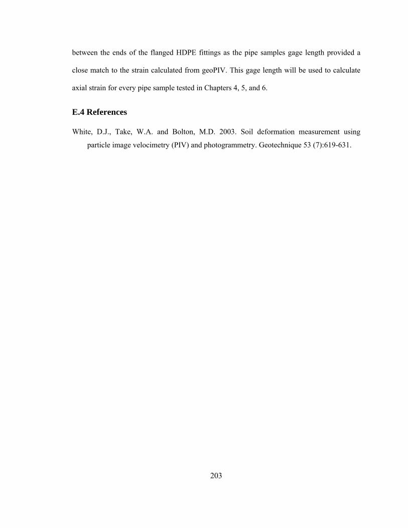
203

between the ends of the flanged HDPE fittings as the pipe samples gage length provided a

close match to the strain calculated from geoPIV. This gage length will be used to calculate

axial strain for every pipe sample tested in Chapters 4, 5, and 6.

E.4 References

White, D.J., Take, W.A. and Bolton, M.D. 2003. Soil deformation measurement using

particle image velocimetry (PIV) and photogrammetry. Geotechnique 53 (7):619-631.

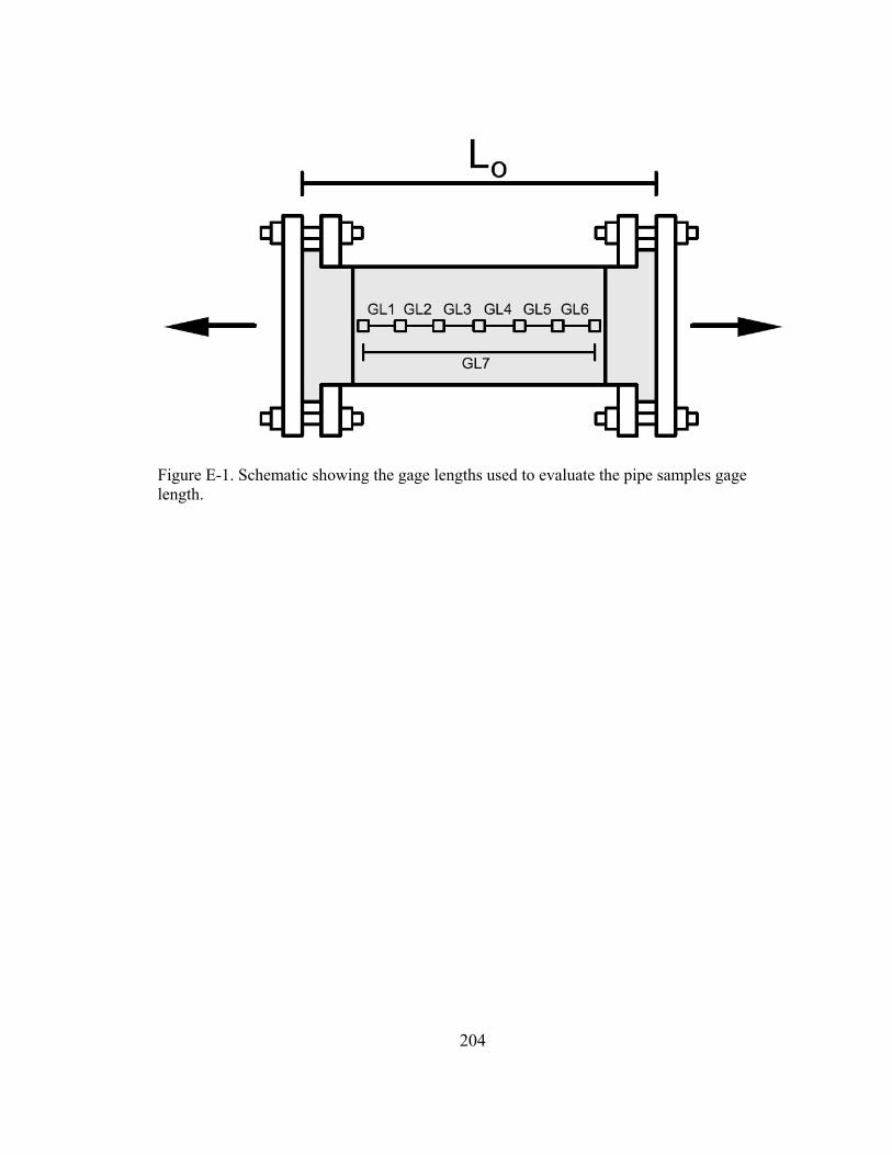
204

Figure E-1. Schematic showing the gage lengths used to evaluate the pipe samples gage length.

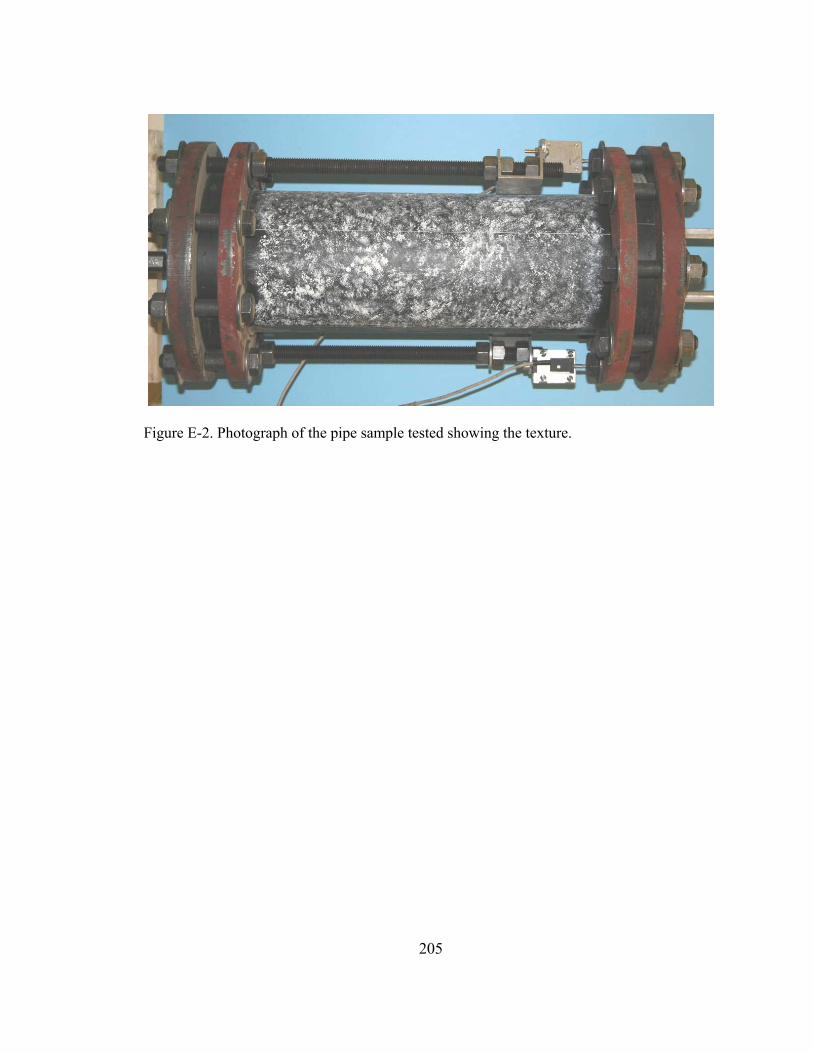
205

Figure E-2. Photograph of the pipe sample tested showing the texture.

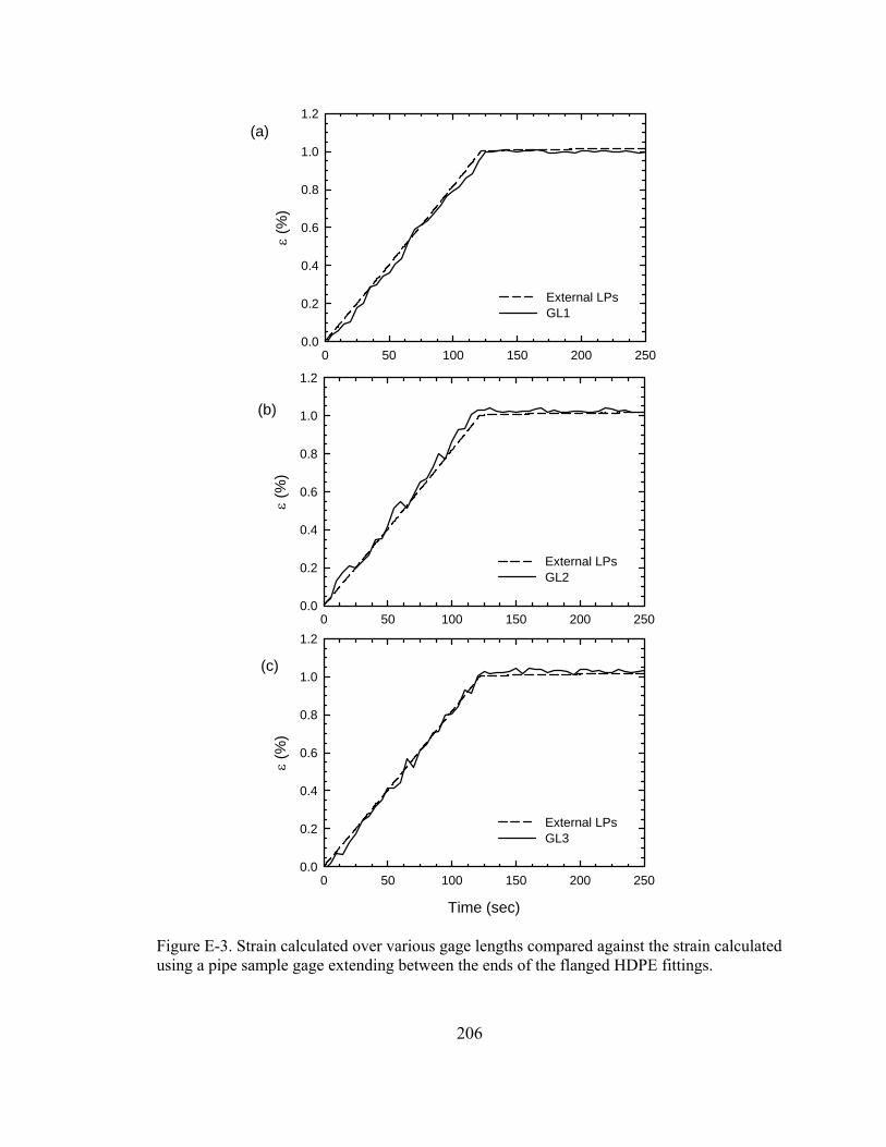
206

0 50 100 150 200 250

ε (%

)

0.0

0.2

0.4

0.6

0.8

1.0

1.2

External LPsGL1

0 50 100 150 200 250

ε (%

)

0.0

0.2

0.4

0.6

0.8

1.0

1.2

External LPsGL2

Time (sec)

0 50 100 150 200 250

ε (%

)

0.0

0.2

0.4

0.6

0.8

1.0

1.2

External LPsGL3

(a)

(b)

(c)

Figure E-3. Strain calculated over various gage lengths compared against the strain calculated using a pipe sample gage extending between the ends of the flanged HDPE fittings.

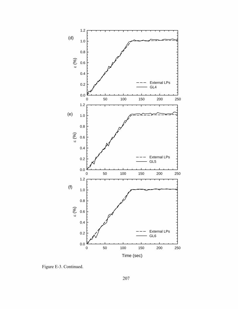
207

0 50 100 150 200 250

ε (%

)

0.0

0.2

0.4

0.6

0.8

1.0

1.2

External LPsGL4

0 50 100 150 200 250

ε (%

)

0.0

0.2

0.4

0.6

0.8

1.0

1.2

External LPsGL5

Time (sec)

0 50 100 150 200 250

ε (%

)

0.0

0.2

0.4

0.6

0.8

1.0

1.2

External LPsGL6

(d)

(e)

(f)

Figure E-3. Continued.

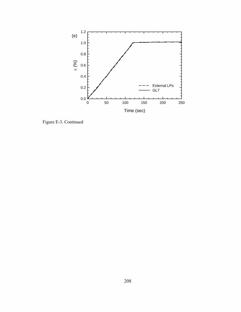
208

Time (sec)

0 50 100 150 200 250

ε (%

)

0.0

0.2

0.4

0.6

0.8

1.0

1.2

External LPsGL7

(e)

Figure E-3. Continued

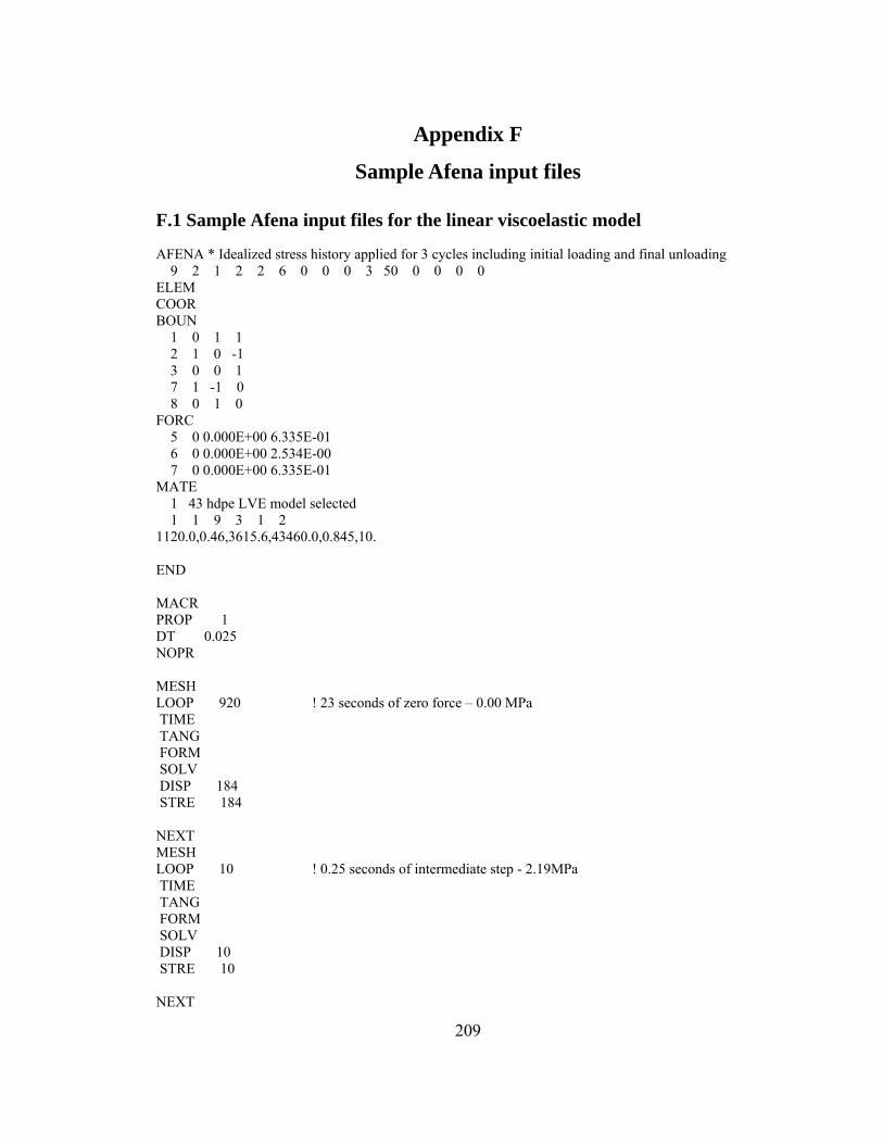
209

Appendix F

Sample Afena input files

F.1 Sample Afena input files for the linear viscoelastic model

AFENA * Idealized stress history applied for 3 cycles including initial loading and final unloading 9 2 1 2 2 6 0 0 0 3 50 0 0 0 0 ELEM COOR BOUN 1 0 1 1 2 1 0 -1 3 0 0 1 7 1 -1 0 8 0 1 0 FORC 5 0 0.000E+00 6.335E-01 6 0 0.000E+00 2.534E-00 7 0 0.000E+00 6.335E-01 MATE 1 43 hdpe LVE model selected 1 1 9 3 1 2 1120.0,0.46,3615.6,43460.0,0.845,10. END MACR PROP 1 DT 0.025 NOPR MESH LOOP 920 ! 23 seconds of zero force – 0.00 MPa TIME TANG FORM SOLV DISP 184 STRE 184 NEXT MESH LOOP 10 ! 0.25 seconds of intermediate step - 2.19MPa TIME TANG FORM SOLV DISP 10 STRE 10 NEXT

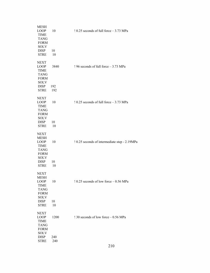
210

MESH LOOP 10 ! 0.25 seconds of full force – 3.73 MPa TIME TANG FORM SOLV DISP 10 STRE 10 NEXT LOOP 3840 ! 96 seconds of full force – 3.73 MPa TIME TANG FORM SOLV DISP 192 STRE 192 NEXT LOOP 10 ! 0.25 seconds of full force – 3.73 MPa TIME TANG FORM SOLV DISP 10 STRE 10 NEXT MESH LOOP 10 ! 0.25 seconds of intermediate step - 2.19MPa TIME TANG FORM SOLV DISP 10 STRE 10 NEXT MESH LOOP 10 ! 0.25 seconds of low force – 0.56 MPa TIME TANG FORM SOLV DISP 10 STRE 10 NEXT LOOP 1200 ! 30 seconds of low force – 0.56 MPa TIME TANG FORM SOLV DISP 240 STRE 240

211

NEXT MESH LOOP 10 ! 0.25 seconds of intermediate step - 2.19MPa TIME TANG FORM SOLV DISP 10 STRE 10 NEXT MESH LOOP 10 ! 0.25 seconds of full force – 3.73 MPa TIME TANG FORM SOLV DISP 10 STRE 10 NEXT LOOP 4760 ! 119 seconds of full force – 3.73 MPa TIME TANG FORM SOLV DISP 170 STRE 170 NEXT LOOP 10 ! 0.25 seconds of full force – 3.73 MPa TIME TANG FORM SOLV DISP 10 STRE 10 NEXT MESH LOOP 10 ! 0.25 seconds of intermediate step - 2.19MPa TIME TANG FORM SOLV DISP 10 STRE 10 NEXT MESH LOOP 10 ! 30 seconds of low force – 0.56 MPa TIME TANG FORM

212

SOLV DISP 10 STRE 10 NEXT LOOP 1200 ! 30 seconds of low force – 0.56 MPa TIME TANG FORM SOLV DISP 240 STRE 240 NEXT MESH LOOP 10 ! 0.25 seconds of intermediate step - 2.19MPa TIME TANG FORM SOLV DISP 10 STRE 10 NEXT MESH LOOP 10 ! 0.25 seconds of full force – 3.73 MPa TIME TANG FORM SOLV DISP 10 STRE 10 NEXT LOOP 4760 ! 119 seconds of full force – 3.73 MPa TIME TANG FORM SOLV DISP 170 STRE 170 NEXT LOOP 10 !0.25 seconds of full force – 3.73 MPa TIME TANG FORM SOLV DISP 10 STRE 10 NEXT MESH LOOP 10 !0.25 seconds of intermediate step - 2.19MPa TIME

213

TANG FORM SOLV DISP 10 STRE 10 NEXT MESH LOOP 48000 ! 1200 seconds of zero force TIME TANG FORM SOLV DISP 1000 STRE 1000 NEXT LOOP 48000 ! 1200 seconds of zero force TIME TANG FORM SOLV DISP 1000 STRE 1000 NEXT LOOP 48000 ! 1200 seconds of zero force TIME TANG FORM SOLV DISP 1000 STRE 1000 NEXT END 1,0,0,1.E6,1.,0.,0.,0.,0. FORC set forces to 0.00 MPa 5 0 0.000E+00 1.667E-10 6 0 0.000E+00 6.667E-10 7 0 0.000E+00 1.667E-10 END FORC set forces to 2.19 MPa 5 0 0.000E+00 3.650E-01 6 0 0.000E+00 1.460E-00 7 0 0.000E+00 3.650E-01 END FORC set forces to 3.73 MPa 5 0 0.000E+00 6.216E-01 6 0 0.000E+00 2.487E-00

214

7 0 0.000E+00 6.216E-01 END FORC set forces to 2.19 MPa 5 0 0.000E+00 3.650E-01 6 0 0.000E+00 1.460E-00 7 0 0.000E+00 3.650E-01 END FORC set forces to 0.56 MPa 5 0 0.000E+00 0.933E-01 6 0 0.000E+00 3.733E-01 7 0 0.000E+00 0.933E-01 END FORC set forces to 2.19 MPa 5 0 0.000E+00 3.650E-01 6 0 0.000E+00 1.460E-00 7 0 0.000E+00 3.650E-01 END FORC set forces to 3.73 MPa 5 0 0.000E+00 6.216E-01 6 0 0.000E+00 2.487E-00 7 0 0.000E+00 6.216E-01 END FORC set forces to 2.19 MPa 5 0 0.000E+00 3.650E-01 6 0 0.000E+00 1.460E-00 7 0 0.000E+00 3.650E-01 END FORC set forces to 0.56 MPa 5 0 0.000E+00 0.933E-01 6 0 0.000E+00 3.733E-01 7 0 0.000E+00 0.933E-01 END FORC set forces to 2.19 MPa 5 0 0.000E+00 3.650E-01 6 0 0.000E+00 1.460E-00 7 0 0.000E+00 3.650E-01 END FORC set forces to 3.73 MPa 5 0 0.000E+00 6.216E-01

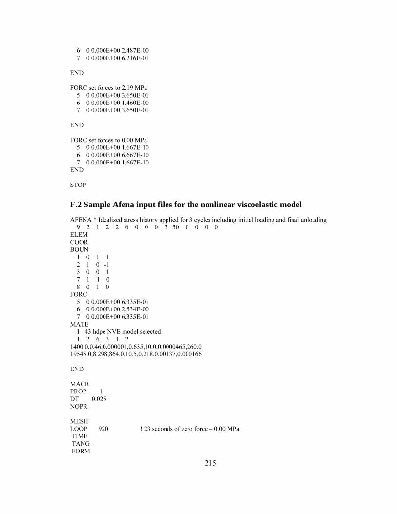
215

6 0 0.000E+00 2.487E-00 7 0 0.000E+00 6.216E-01 END FORC set forces to 2.19 MPa 5 0 0.000E+00 3.650E-01 6 0 0.000E+00 1.460E-00 7 0 0.000E+00 3.650E-01 END FORC set forces to 0.00 MPa 5 0 0.000E+00 1.667E-10 6 0 0.000E+00 6.667E-10 7 0 0.000E+00 1.667E-10 END STOP F.2 Sample Afena input files for the nonlinear viscoelastic model

AFENA * Idealized stress history applied for 3 cycles including initial loading and final unloading 9 2 1 2 2 6 0 0 0 3 50 0 0 0 0 ELEM COOR BOUN 1 0 1 1 2 1 0 -1 3 0 0 1 7 1 -1 0 8 0 1 0 FORC 5 0 0.000E+00 6.335E-01 6 0 0.000E+00 2.534E-00 7 0 0.000E+00 6.335E-01 MATE 1 43 hdpe NVE model selected 1 2 6 3 1 2 1400.0,0.46,0.000001,0.635,10.0,0.0000465,260.0 19545.0,8.298,864.0,10.5,0.218,0.00137,0.000166 END MACR PROP 1 DT 0.025 NOPR MESH LOOP 920 ! 23 seconds of zero force – 0.00 MPa TIME TANG FORM

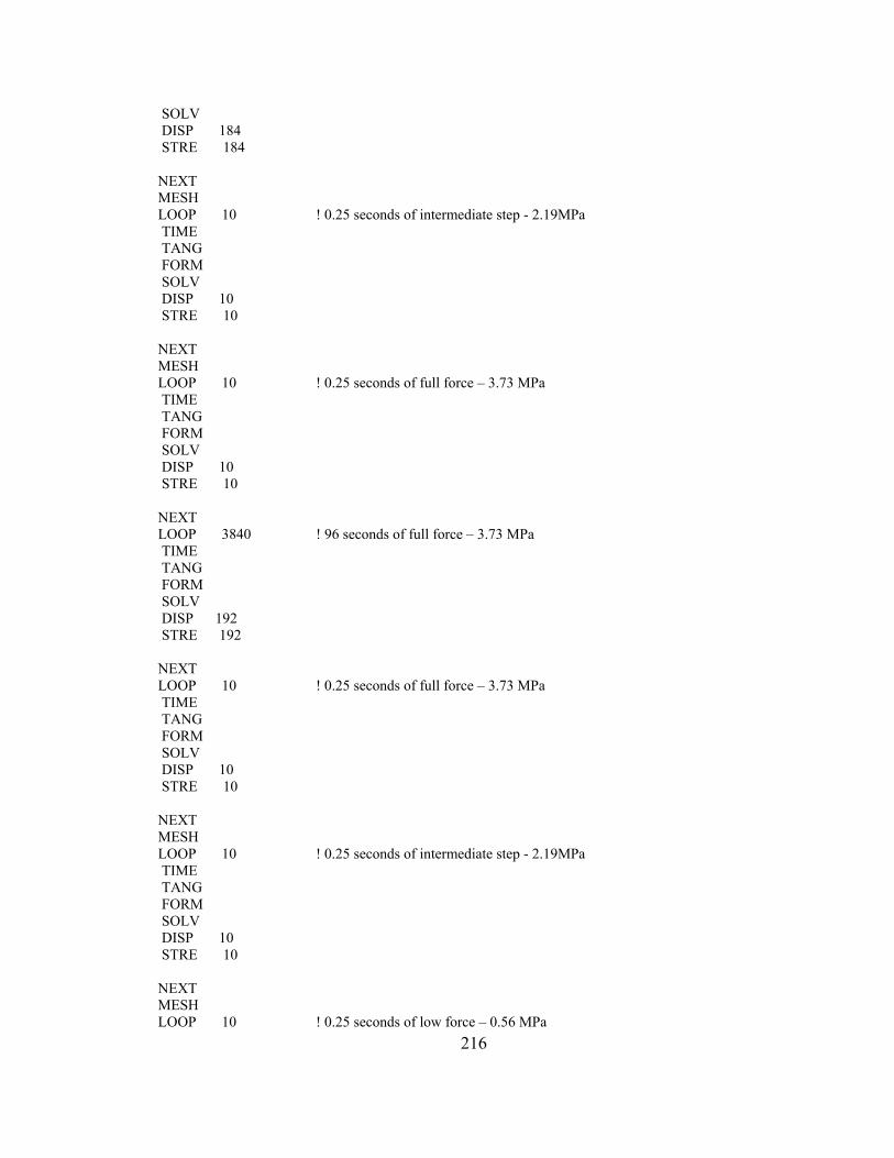
216

SOLV DISP 184 STRE 184 NEXT MESH LOOP 10 ! 0.25 seconds of intermediate step - 2.19MPa TIME TANG FORM SOLV DISP 10 STRE 10 NEXT MESH LOOP 10 ! 0.25 seconds of full force – 3.73 MPa TIME TANG FORM SOLV DISP 10 STRE 10 NEXT LOOP 3840 ! 96 seconds of full force – 3.73 MPa TIME TANG FORM SOLV DISP 192 STRE 192 NEXT LOOP 10 ! 0.25 seconds of full force – 3.73 MPa TIME TANG FORM SOLV DISP 10 STRE 10 NEXT MESH LOOP 10 ! 0.25 seconds of intermediate step - 2.19MPa TIME TANG FORM SOLV DISP 10 STRE 10 NEXT MESH LOOP 10 ! 0.25 seconds of low force – 0.56 MPa

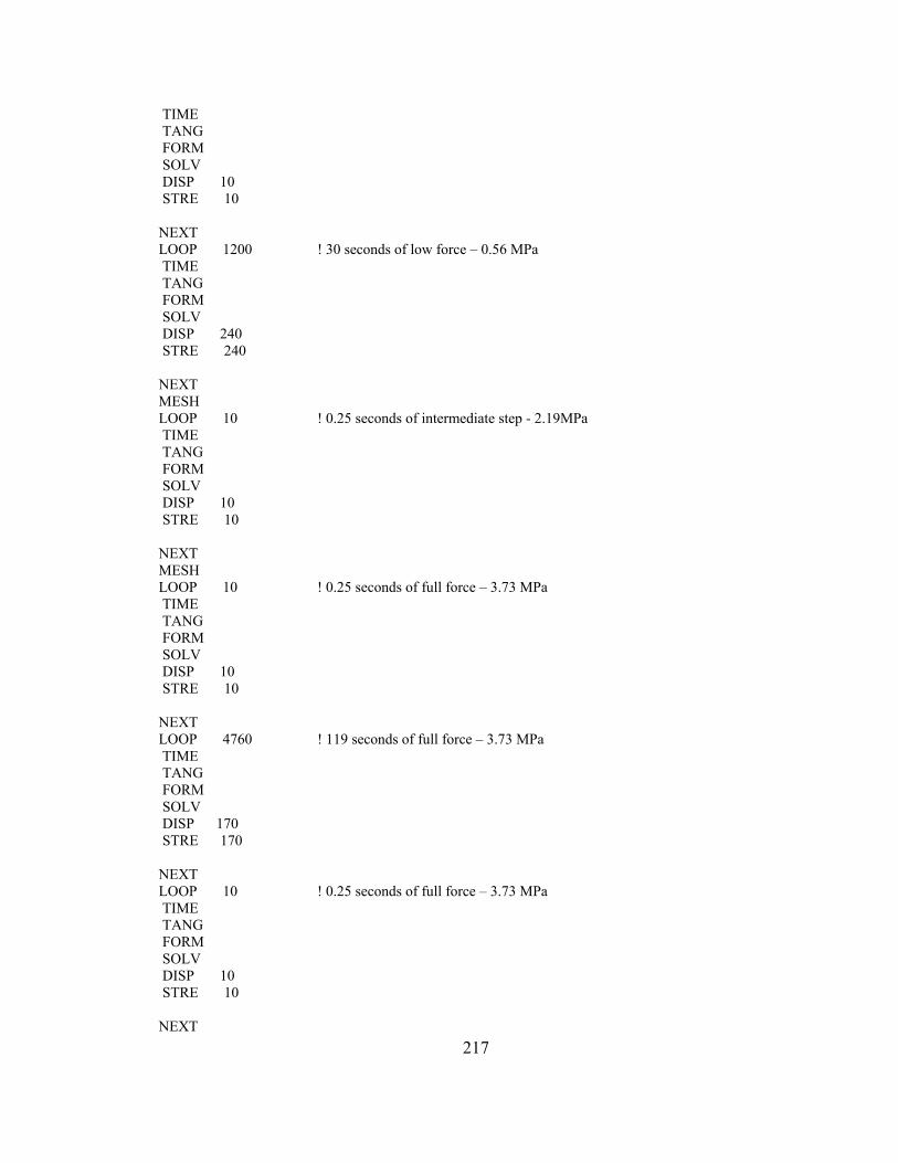
217

TIME TANG FORM SOLV DISP 10 STRE 10 NEXT LOOP 1200 ! 30 seconds of low force – 0.56 MPa TIME TANG FORM SOLV DISP 240 STRE 240 NEXT MESH LOOP 10 ! 0.25 seconds of intermediate step - 2.19MPa TIME TANG FORM SOLV DISP 10 STRE 10 NEXT MESH LOOP 10 ! 0.25 seconds of full force – 3.73 MPa TIME TANG FORM SOLV DISP 10 STRE 10 NEXT LOOP 4760 ! 119 seconds of full force – 3.73 MPa TIME TANG FORM SOLV DISP 170 STRE 170 NEXT LOOP 10 ! 0.25 seconds of full force – 3.73 MPa TIME TANG FORM SOLV DISP 10 STRE 10 NEXT

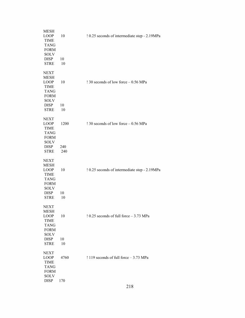
218

MESH LOOP 10 ! 0.25 seconds of intermediate step - 2.19MPa TIME TANG FORM SOLV DISP 10 STRE 10 NEXT MESH LOOP 10 ! 30 seconds of low force – 0.56 MPa TIME TANG FORM SOLV DISP 10 STRE 10 NEXT LOOP 1200 ! 30 seconds of low force – 0.56 MPa TIME TANG FORM SOLV DISP 240 STRE 240 NEXT MESH LOOP 10 ! 0.25 seconds of intermediate step - 2.19MPa TIME TANG FORM SOLV DISP 10 STRE 10 NEXT MESH LOOP 10 ! 0.25 seconds of full force – 3.73 MPa TIME TANG FORM SOLV DISP 10 STRE 10 NEXT LOOP 4760 ! 119 seconds of full force – 3.73 MPa TIME TANG FORM SOLV DISP 170

219

STRE 170 NEXT LOOP 10 !0.25 seconds of full force – 3.73 MPa TIME TANG FORM SOLV DISP 10 STRE 10 NEXT MESH LOOP 10 !0.25 seconds of intermediate step - 2.19MPa TIME TANG FORM SOLV DISP 10 STRE 10 NEXT MESH LOOP 48000 ! 1200 seconds of zero force TIME TANG FORM SOLV DISP 1000 STRE 1000 NEXT LOOP 48000 ! 1200 seconds of zero force TIME TANG FORM SOLV DISP 1000 STRE 1000 NEXT LOOP 48000 ! 1200 seconds of zero force TIME TANG FORM SOLV DISP 1000 STRE 1000 NEXT END 1,0,0,1.E6,1.,0.,0.,0.,0. FORC set forces to 0.00 MPa 5 0 0.000E+00 1.667E-10

220

6 0 0.000E+00 6.667E-10 7 0 0.000E+00 1.667E-10 END FORC set forces to 2.19 MPa 5 0 0.000E+00 3.650E-01 6 0 0.000E+00 1.460E-00 7 0 0.000E+00 3.650E-01 END FORC set forces to 3.73 MPa 5 0 0.000E+00 6.216E-01 6 0 0.000E+00 2.487E-00 7 0 0.000E+00 6.216E-01 END FORC set forces to 2.19 MPa 5 0 0.000E+00 3.650E-01 6 0 0.000E+00 1.460E-00 7 0 0.000E+00 3.650E-01 END FORC set forces to 0.56 MPa 5 0 0.000E+00 0.933E-01 6 0 0.000E+00 3.733E-01 7 0 0.000E+00 0.933E-01 END FORC set forces to 2.19 MPa 5 0 0.000E+00 3.650E-01 6 0 0.000E+00 1.460E-00 7 0 0.000E+00 3.650E-01 END FORC set forces to 3.73 MPa 5 0 0.000E+00 6.216E-01 6 0 0.000E+00 2.487E-00 7 0 0.000E+00 6.216E-01 END FORC set forces to 2.19 MPa 5 0 0.000E+00 3.650E-01 6 0 0.000E+00 1.460E-00 7 0 0.000E+00 3.650E-01 END FORC set forces to 0.56 MPa

221

5 0 0.000E+00 0.933E-01 6 0 0.000E+00 3.733E-01 7 0 0.000E+00 0.933E-01 END FORC set forces to 2.19 MPa 5 0 0.000E+00 3.650E-01 6 0 0.000E+00 1.460E-00 7 0 0.000E+00 3.650E-01 END

FORC set forces to 3.73 MPa 5 0 0.000E+00 6.216E-01 6 0 0.000E+00 2.487E-00 7 0 0.000E+00 6.216E-01 END

FORC set forces to 2.19 MPa 5 0 0.000E+00 3.650E-01 6 0 0.000E+00 1.460E-00 7 0 0.000E+00 3.650E-01 END FORC set forces to 0.00 MPa 5 0 0.000E+00 1.667E-10 6 0 0.000E+00 6.667E-10 7 0 0.000E+00 1.667E-10 END STOP

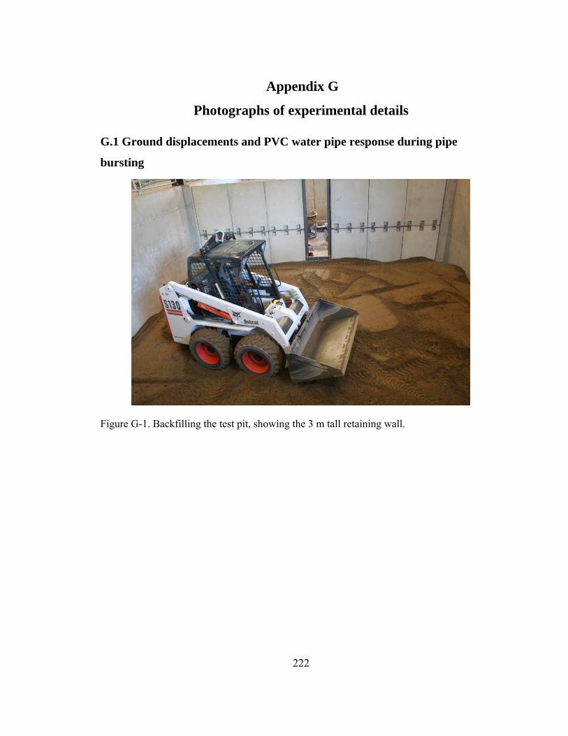
222

Appendix G

Photographs of experimental details

G.1 Ground displacements and PVC water pipe response during pipe

bursting

Figure G-1. Backfilling the test pit, showing the 3 m tall retaining wall.

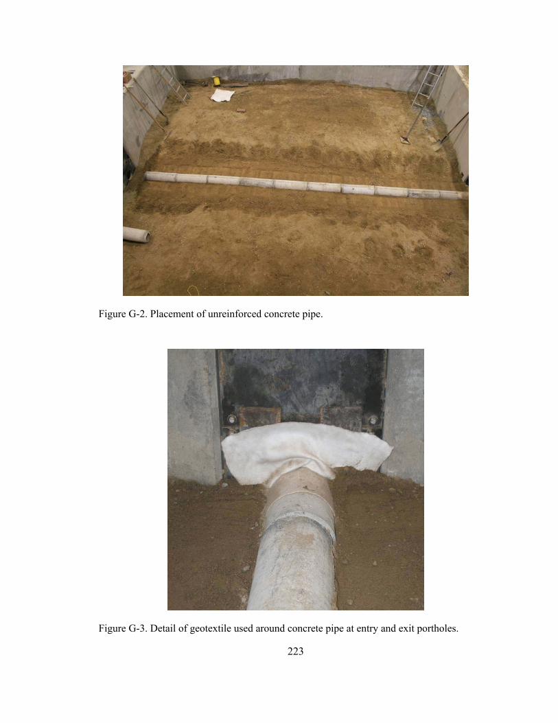
223

Figure G-2. Placement of unreinforced concrete pipe.

Figure G-3. Detail of geotextile used around concrete pipe at entry and exit portholes.

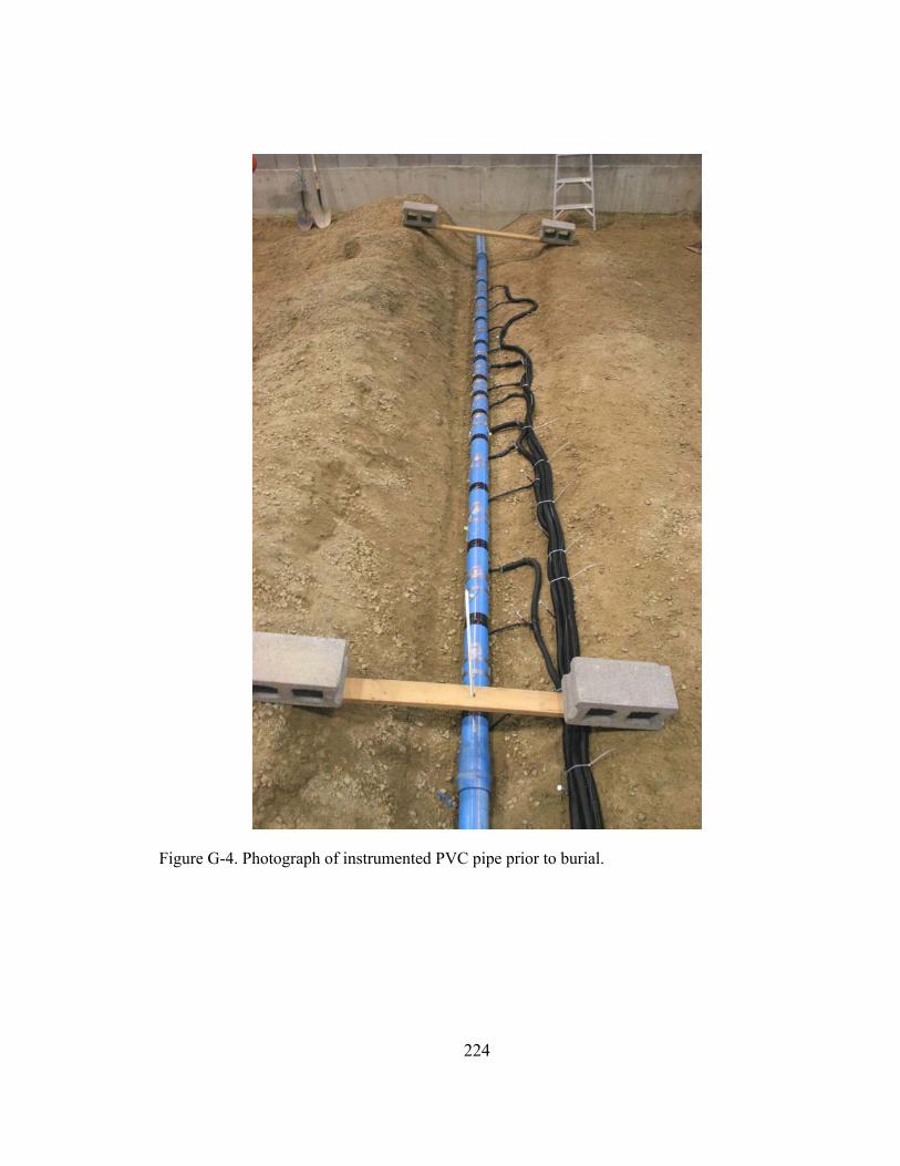
224

Figure G-4. Photograph of instrumented PVC pipe prior to burial.

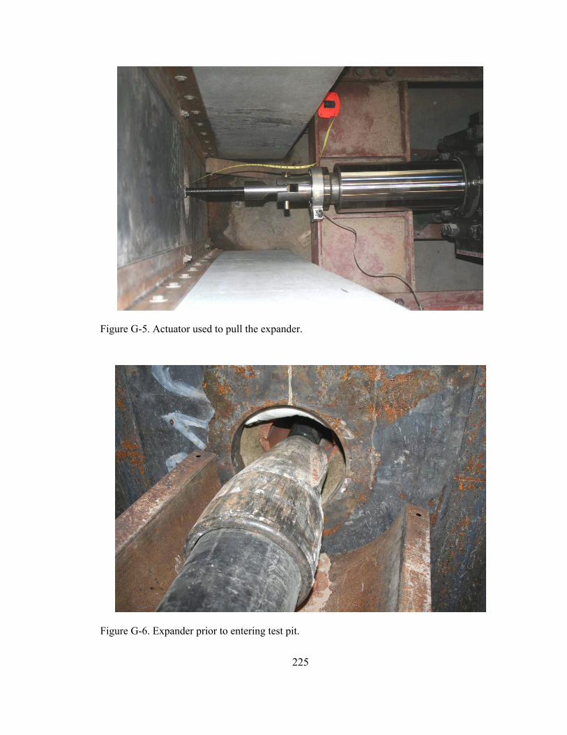
225

Figure G-5. Actuator used to pull the expander.

Figure G-6. Expander prior to entering test pit.

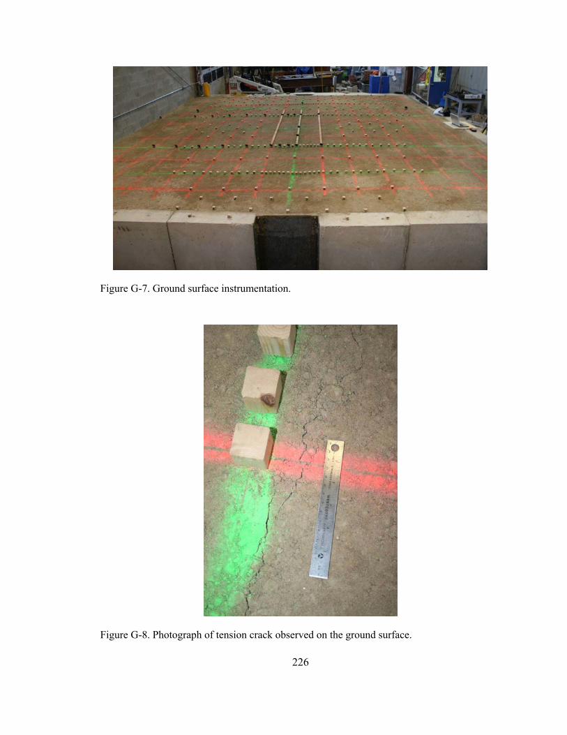
226

Figure G-7. Ground surface instrumentation.

Figure G-8. Photograph of tension crack observed on the ground surface.

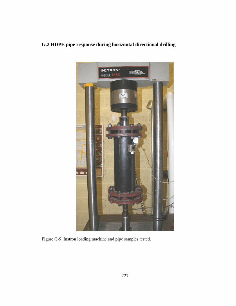
227

G.2 HDPE pipe response during horizontal directional drilling

Figure G-9. Instron loading machine and pipe samples tested.

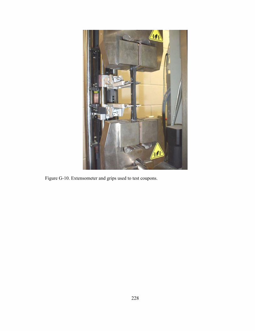
228

Figure G-10. Extensometer and grips used to test coupons.