transient analysis in pipe networks
TRANSCRIPT
TRANSIENT ANALYSIS IN PIPE NETWORKS
Kishore Sirvole
Thesis submitted to the Faculty of the
Virginia Polytechnic Institute & State University
In partial fulfillment of the requirements for the degree of
MASTER OF SCIENCE
in
Civil Engineering
Approved:
Vinod K. Lohani, Co-Chair
David F. Kibler, Co-Chair Tamim Younos, Member
September 25, 2007
Blacksburg, Virginia
Key Words: Method of characteristics, Water hammer, Transient analysis, Gaseous cavitation, Object oriented programming.
Trasnient analysis in pipe networks
Kishore Sirvole
Abstract
Power failure of pumps, sudden valve actions, and the operation of automatic control systems are
all capable of generating high pressure waves in domestic water supply systems. These transient
conditions resulting in high pressures can cause pipe failures by damaging valves and fittings. In
this study, basic equations for solving transient analysis problems are derived using method of
characteristics. Two example problems are presented. One, a single pipe system which is solved
by developing an excel spreadsheet. Second, a pipe network problem is solved using transient
analysis program called TRANSNET.
A transient analysis program is developed in Java. This program can handle suddenly-closing
valves, gradually-closing valves, pump power failures and sudden demand changes at junctions.
A maximum of four pipes can be present at a junction. A pipe network problem is solved using
this java program and the results were found to be similar to that obtained from TRANSNET
program. The code can be further extended, for example by developing java applets and
graphical user interphase to make it more user friendly.
A two dimensional (2D) numerical model is developed using MATLAB to analyze gaseous
cavitation in a single pipe system. The model is based on mathematical formulations proposed by
Cannizzaro and Pezzinga (2005) and Pezzinga (2003). The model considers gaseous cavitation
due to both thermic exhange between gas bubbles and surrounding liquid and during the process
of gas release. The results from the model show that during transients, there is significant
increase in fluid temperature along with high pressures. In literature pipe failures and noise
problems in premise plumbing are attributed to gaseous cavitation.

iii
Acknowledgments
I would like to thank my committee co-chair Dr. Lohani for his valuable guidance and comments. I am
grateful to Dr. Kibler, also co-chair, for being part of my committee and helping me with my thesis
work. I would like to thank Dr. Tamim Younos for being part of my committee. I am indebted to
Department of Civil Engineering at Virginia Tech. I sincerely thank my friends Vinod, Vyas and Kiran
for their support and companionship.
Last, my sincere regards to my late advisor Dr. Loganathan for selection of this topic and for his
encouragement throughout my graduate study.
iv
Table of Contents
Chapter 1: Introduction ................................................................................................. 1 1.1 Literature Review............................................................................................................................ 1 1.2 Objective ......................................................................................................................................... 2 1.3 Organization
.................................................................................................................................... 2
Chapter 2: Basic Equations of Transient Flow Analysis in Closed Conduits .......... 4 2.1 Introduction ..................................................................................................................................... 4 2.2 Unsteady Flow Equations ............................................................................................................... 4 2.2.1 The Euler Equation ...................................................................................................................... 4 2.2.2 Conservation of Mass .................................................................................................................. 6 2.3 Method of characteristics ................................................................................................................ 9 2.3.1 Finite Difference Approximation:.............................................................................................. 10 2.4. Summary of Equations ................................................................................................................. 12 2.5 Boundary Conditions .................................................................................................................... 15 2.5.1 Reservoir .................................................................................................................................... 15 2.5.2 Valve .......................................................................................................................................... 15 2.5.3 Pumps and Turbines ................................................................................................................... 16 2.5.4 Junctions .................................................................................................................................... 16 2.6 Transient Flow Analysis ............................................................................................................... 18 2.6.1 Single pipe system ..................................................................................................................... 18 2.6.2 Network Distribution
................................................................................................................. 23
Chapter 3: An Object Oriented Approach for Transient Analysis in Water Distribution Systems using JAVA programming ...................................................... 27
3.1 Introduction ................................................................................................................................... 27 3.2 Object-oriented programming in Java .......................................................................................... 29 3.3 Object oriented design .................................................................................................................. 31 3.4 Classes used in Object oriented program ...................................................................................... 32 3.5 Comparison between TRANSNET and JAVA ............................................................................. 36 3.6 Test problem and Verification of Results
..................................................................................... 38
Chapter 4: Modeling Transient Gaseous Cavitation in Pipes .................................. 40 4.1 Introduction ................................................................................................................................... 40 4.2 Free Gas in Liquids ....................................................................................................................... 41 4.3 Rate of Gas Release ...................................................................................................................... 42 4.4 Energy Equation of gas as function of Temperature and Pressure ............................................... 43 4.4.1 Relation between and ....................................................................................................... 44 4.4.2 Newton’s law of cooling ............................................................................................................ 46 4.5 One-Dimensional Two-Phase Flow .............................................................................................. 47 4.5.1 Mixture Density ......................................................................................................................... 47 4.5.2 Continuity Equation
pc
................................................................................................................... 48
vc
v
4.6 Conservation form of Mixture Continuity and Energy Equations ................................................ 49 4.7 Mixture Momentum Equation ....................................................................................................... 50 4.7.1 Stress Model............................................................................................................................... 51 4.7.2 Evaluating Thickness of Viscous Sub layer ............................................................................... 52 4.7.3 Boundary Conditions ................................................................................................................. 53 4.8 Finite Difference Scheme .......................................................................................................... 53 4.8.1 Mac’cormack Method ................................................................................................................ 54 4.9 Application of the Model
.............................................................................................................. 57
Chapter 5: Summary and Conclusions ...................................................................... 61 5.1 Summary ....................................................................................................................................... 61 5.2 Conclusion
.................................................................................................................................... 62
Appendix A-1: Steady state analysis results………………………………………………………..63 Appendix A-2: Transient analysis results…………………………………………………………..68 Appendix B: Comparison between WHAMO and TRANSNET results…………………………...77 Appendix C-1: Java program input………………………………………………………………...79 Appendix C-2: Java program output……………………………………………………………….80
Appendix D: Matlab program……………………………………………………………………..84
References:
.................................................................................................................. 107
vi
List of Figures
Figure 1. Cylindrical fluid element with all forces shown. ................................................................... 4 Figure 2. Control volume coinciding with the interior surface of the pipe ........................................... 6 Figure 3 Parameters in the interpolation procedure. ........................................................................... 10 Figure 4. Characterstics shown on a finite difference grid ................................................................ 14 Figure 5 Four pipe junction with valve downstream of one pipe ....................................................... 16 Figure 6. Single pipeline with reservoir upstream and valve downstream ......................................... 19 Figure 7. Single pipe with reservoir upstream and valve downstream ............................................... 21 Figure 8. Network distribution system................................................................................................ 23 Figure 9. Different types of programming methods ........................................................................... 29 Figure 10. Flow chart to solve for pressure and velocity heads using method of characteristics ....... 30 Figure 11. UML class diagram ........................................................................................................... 31 Figure 12. Shear stress distribution and velocity profile for turbulent flow ....................................... 52 Figure 13. Cylindrical grid element .................................................................................................... 54 Figure 14. 2-D Finite difference grid .................................................................................................. 54 Figure 15. Flow chart to show steps for modeling gaseous cavitation ............................................... 56 Figure 16. Head vs Time plot near the valve ...................................................................................... 58 Figure 17. Temperature vs Time plot near the valve ......................................................................... 59
Figure 18. Mass of released gas vs time plot near the valve ............................................................... 59
List of Tables
Table 1. Transient analysis of single pipe system using method of characteristics ............................ 20 Table 2. Pipe data ................................................................................................................................ 23 Table 3. Node data .............................................................................................................................. 24 Table 4. Pipe data-results of steady flow analysis .............................................................................. 24 Table 5. Node data-results of steady flow analysis ............................................................................. 24 Table 6. Results of transient flow anaysis at pipe 5 ............................................................................ 25 Table 7. Relationships between classes .............................................................................................. 32 Table 8. Methods in Pipe class ........................................................................................................... 33 Table 9. Methods in Pressure Analyser class...................................................................................... 34 Table 10: Methods in Pump class ....................................................................................................... 35 Table 11: Methods in Reservoir Junction class .................................................................................. 35 Table 12: Methods in Standard Junction class .................................................................................... 36 Table 13. Comparative advantages of the object- oriented programming .......................................... 38 Table 14. Maximum pressure head (in feet) values during transients in pipe network ...................... 38
Table 15. Data used by gaseous cavitation model .............................................................................. 57
vii
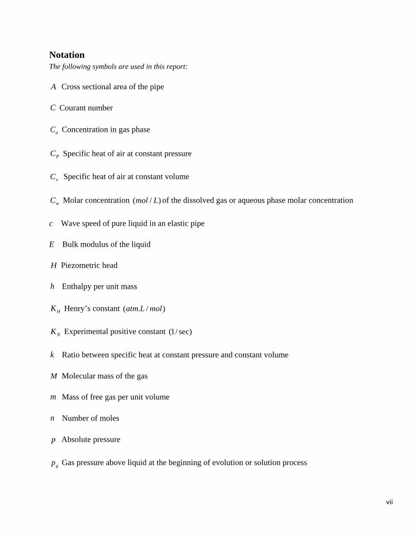
Notation The following symbols are used in this report:
A Cross sectional area of the pipe
C Courant number
aC Concentration in gas phase
PC Specific heat of air at constant pressure
vC Specific heat of air at constant volume
wC Molar concentration )/( Lmol of the dissolved gas or aqueous phase molar concentration
c Wave speed of pure liquid in an elastic pipe
E Bulk modulus of the liquid
H Piezometric head
h Enthalpy per unit mass
HK Henry’s constant )/.( molLatm
NK Experimental positive constant sec)/1(
k Ratio between specific heat at constant pressure and constant volume
M Molecular mass of the gas
m Mass of free gas per unit volume
n Number of moles
p Absolute pressure
gp Gas pressure above liquid at the beginning of evolution or solution process
viii
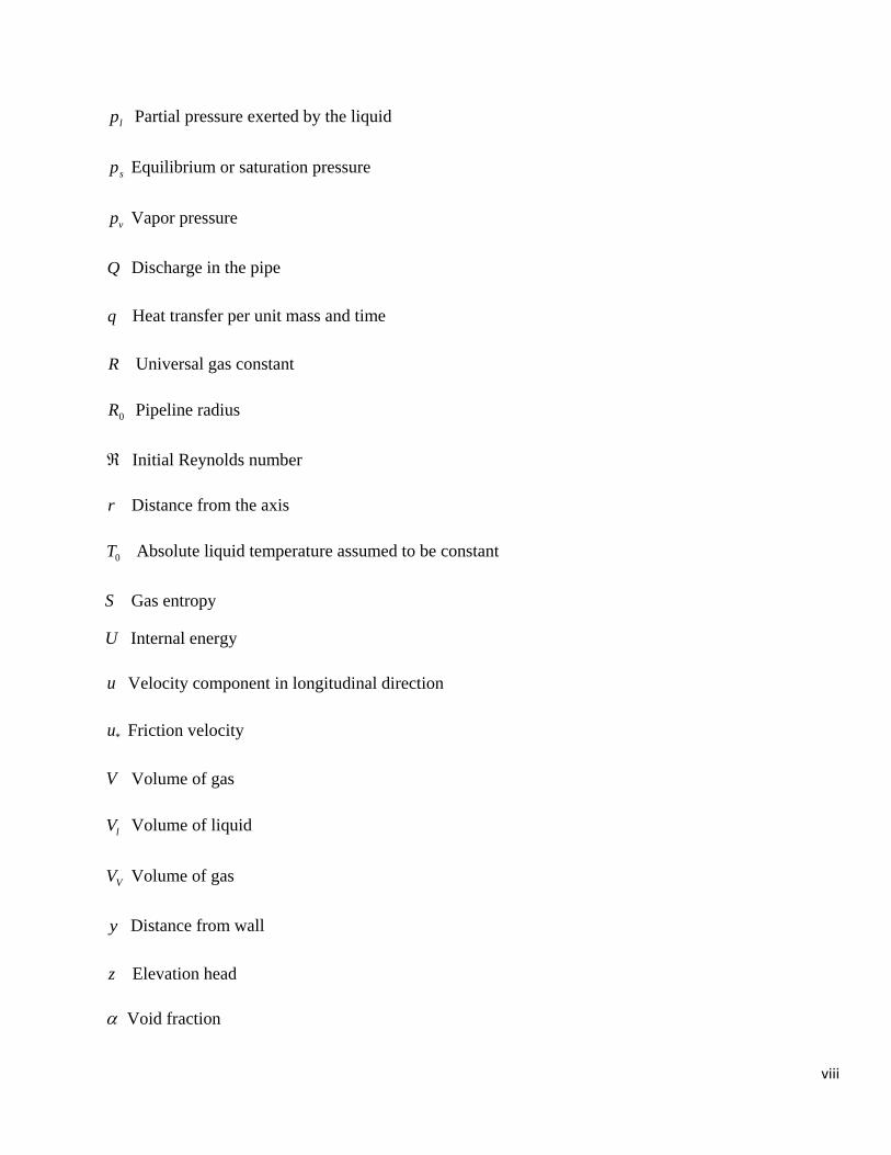
lp Partial pressure exerted by the liquid
sp Equilibrium or saturation pressure
vp Vapor pressure
Q Discharge in the pipe
q Heat transfer per unit mass and time
R Universal gas constant
0R Pipeline radius
ℜ Initial Reynolds number
r Distance from the axis
0T Absolute liquid temperature assumed to be constant
S Gas entropy
U Internal energy
u Velocity component in longitudinal direction
*u Friction velocity
V Volume of gas
lV Volume of liquid
VV Volume of gas
y Distance from wall
z Elevation head
α Void fraction
ix
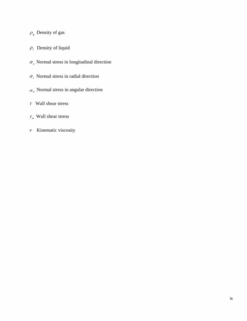
gρ Density of gas
lρ Density of liquid
xσ Normal stress in longitudinal direction
rσ Normal stress in radial direction
θσ Normal stress in angular direction
τ Wall shear stress
wτ Wall shear stress
ν Kinematic viscosity
1
Chapter 1: Introduction Devices such as valves, pumps and surge protection equipment exist in a pipe network. Power failure of
pumps, sudden valve actions, and the operation of automatic control systems are all capable of
generating high pressure waves in domestic water supply systems. These high pressures can cause pipe
failures by damaging valves and fittings. Study of pressure and velocity variations under such
circumstances is significant for placement of valves and other protection devices. In this study, the role
of each of these devices in triggering transient conditions is studied. Analysis is performed on single and
multiple pipe systems.
Transient analysis is also important to draw guidelines for future pipeline design standards. These will
use true maximum loads (pressure and velocity) to select the appropriate components, rather than a
notional factor of the mean operating pressure. This will lead to safer designs with less over-design,
guaranteeing better system control and allowing unconventional solutions such as the omission of
expensive protection devices. It will also reveal potential problems in the operation of the system at the
design stage, at a much lower cost than during commissioning.
1.1 Literature Review
Most of the problems considering unsteady pure liquid flow in pipes are solved using a set of partial
differential equations (Wylie and Streeter, 1993) which are discussed in detail in Chapter 2. These
equations are valid only when the pressure is greater than the vapor pressure of liquid, and are solved
numerically using the method of characteristics which was introduced by Streeter and Wylie (1967). But
in many flow regimes, small amount of free gas is present in a liquid. When local pressure during
transient drops below saturation pressure, the liquid releases free gas. If the pressure drops to vapor
pressure, cavities are formed (Tullis et al., 1976). The former occurrence is called gaseous cavitation
where as the latter occurrence is called vaporous cavitation.
Martin et al., (1976) developed a one-dimensional homogeneous bubbly model using a two step Lax-
Wendroff scheme. Pressure wave propagation and interactions are handled well by Lax-Wendroff
scheme by introducing a pseudo-viscosity term. The results produced by this model compare favorably
with experiment than by using fixed grid method of characteristics. An analytical model was developed
2
by Wiggert and Sundquist (1979) to investigate gaseous cavitation using the method of characteristics.
Gas release is assumed mainly due to difference in local unsteady pressure and saturation pressure.
Increase in void fraction due to latent heat flow is not considered. Wylie (1984) investigated both
gaseous and vapor cavitation using a discrete free gas model. Free gas is lumped at discrete computing
locations and pure liquid is assumed in between these locations. Small void fraction and isothermal
behavior of fluid are some of the assumptions made. Gaseous cavitation is simulated and it gave close
results when compared with other methods. Pezzinga (1999) developed a 2D model, which computes
frictional losses in pipes and pipe networks using instantaneous velocity profiles. The extreme values
for pressure heads and pressure wave oscillations were well reproduced by this model.
Pezzinga (2004) adopted “second viscosity” to better explain energy dissipation during transient gaseous
cavitation. Constant mass of free gas is assumed at constant temperature. Second viscosity or bulk
viscosity coefficient accounts for other forms (other than frictional losses) of energy dissipation such as
gas release and heat exchange between gas bubbles and surrounding liquid.
Cannizzaro and Pezzinga (2005) considered the effects of thermic exchange between gas bubbles and
surrounding liquid and gas release and solution process separately to study energy dissipation during
gaseous cavitation. Separate 2D models were considered. The results of numerical runs shows that 2d
model with gas release allows for a good simulation of the experimental data.
1.2 Objective The objectives of this research are to:
1) Study unsteady flow in pipes and pipe networks carrying pure liquid, including evaluation of
pressure and velocity heads at nodes and junctions at different time intervals,
2) Develop a program using object oriented technology to analyze transients in pipes considering
single phase flow, and
3) Study the effects of gaseous cavitation on fluid transients using equations developed by
Cannizzaro and Pezzinga (2005).
1.3 Organization This thesis is divided into five chapters. Chapter 1 includes a brief introduction to transients, review of
literature, and objectives of the study. Basic equations of transient flow analysis in pipe networks are
3
discussed in Chapter 2. Two example problems are solved using excel spreadsheet to demonstrate the
method of characteristics. Chapter 3 is devoted to use of object oriented technology for analyzing
transient problems in a pipe network. Comparison is drawn between procedural language and object
oriented approach of analyzing transients in a pipe network. Chapter 4 is about gaseous cavitation in
pipes where energy dissipation due to gas release and solution process is studied. Here, thermal
exchange between gas bubbles and surrounding liquid is also considered. A comprehensive model to
obtain the amount of gas release is developed. Chapter 5 presents the summary of work presented in this
thesis, and also discusses its potential application.
4
Chapter 2: Basic Equations of Transient Flow Analysis in Closed Conduits
2.1 Introduction Initial studies on water hammer are done assuming single phase flow of fluid (Wylie et al., 1993). The
method of characteristics is most widely used for modeling water hammer. First, the fundamental
equations involved in water hammer analysis are discussed, following which two example problems are
solved to highlight the analytical technique.
2.2 Unsteady Flow Equations
Study of transient flow includes fluid inertia and also elasticity or compressibility of the fluid and the
conduit. The analysis of transient flow in either of these cases requires the application of Newton’s
second law which leads to the Euler equation as discussed below.
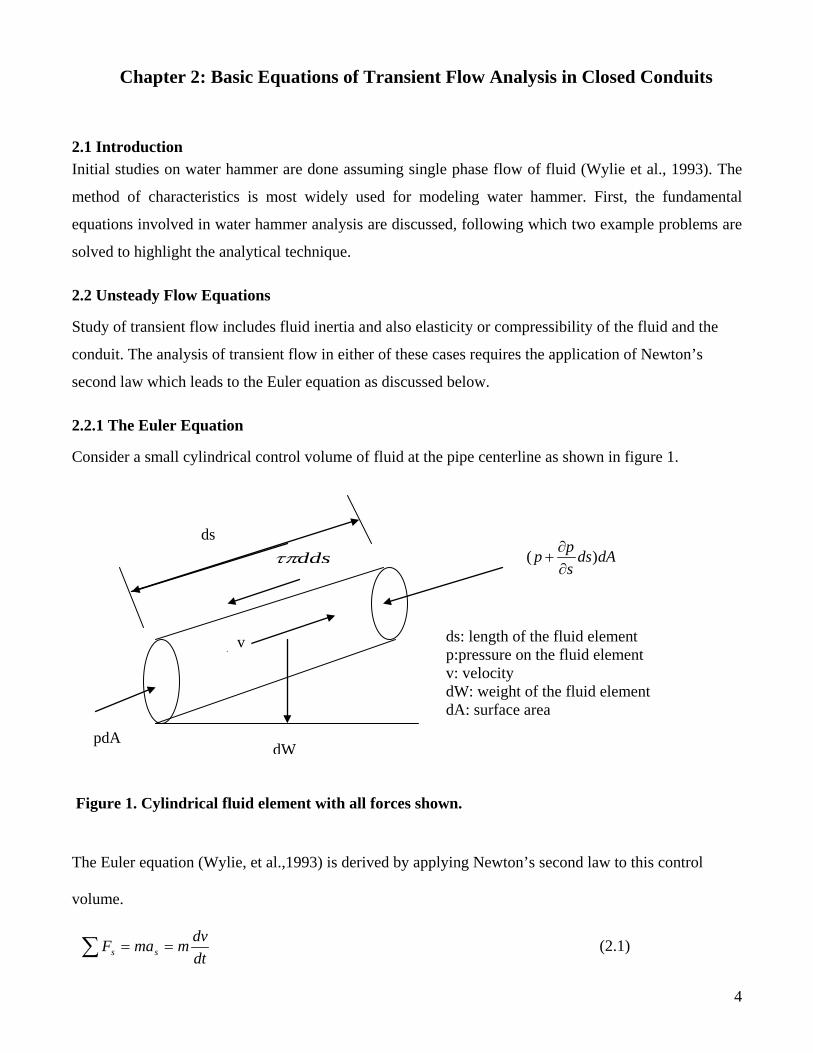
2.2.1 The Euler Equation
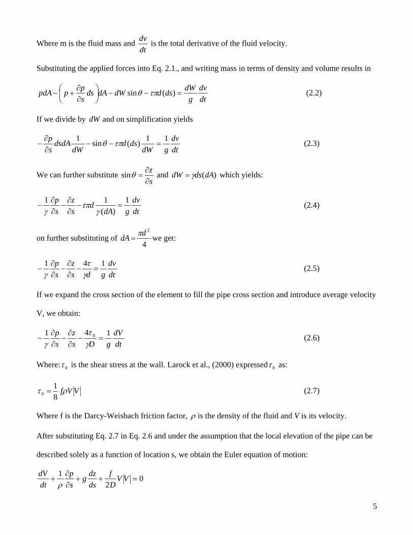
Consider a small cylindrical control volume of fluid at the pipe centerline as shown in figure 1.
Figure 1. Cylindrical fluid element with all forces shown.
The Euler equation (Wylie, et al.,1993) is derived by applying Newton’s second law to this control
volume.
dtdvmmaF ss ==∑ (2.1)
pdA
dAdsspp )(∂∂
+
dW
v
ddsτπ
ds
ds: length of the fluid element p:pressure on the fluid element v: velocity dW: weight of the fluid element dA: surface area
5
Where m is the fluid mass and dtdv is the total derivative of the fluid velocity.
Substituting the applied forces into Eq. 2.1., and writing mass in terms of density and volume results in
dtdv
gdWdsddWdAds
spppdA =−−
∂∂
+− )(sin τπθ (2.2)
If we divide by dW and on simplification yields
dtdv
gdWdsd
dWdsdA
sp 11)(sin1
=−−∂∂
− τπθ (2.3)
We can further substitute sz∂∂
=θsin and )(dAdsdW γ= which yields:
dtdv
gdAd
sz
sp 1
)(11
=−∂∂
−∂∂
−γ
τπγ
(2.4)
on further substituting of 4
2ddA π= we get:
dtdv
gdsz
sp 141
=−∂∂
−∂∂
−γτ
γ (2.5)
If we expand the cross section of the element to fill the pipe cross section and introduce average velocity
V, we obtain:
dtdV
gDsz
sp 141 0 =−
∂∂
−∂∂
−γτ
γ (2.6)
Where: 0τ is the shear stress at the wall. Larock et al., (2000) expressed 0τ as:
VVfρτ81
0 = (2.7)
Where f is the Darcy-Weisbach friction factor, ρ is the density of the fluid and V is its velocity.
After substituting Eq. 2.7 in Eq. 2.6 and under the assumption that the local elevation of the pipe can be
described solely as a function of location s, we obtain the Euler equation of motion:
02
1=++
∂∂
+ VVDf
dsdzg
sp
dtdV
ρ
6
Or,
sVV
tV
∂∂
+∂∂ 0
2sin1
=++∂∂
+ VVDfg
sp α
ρ (2.8)
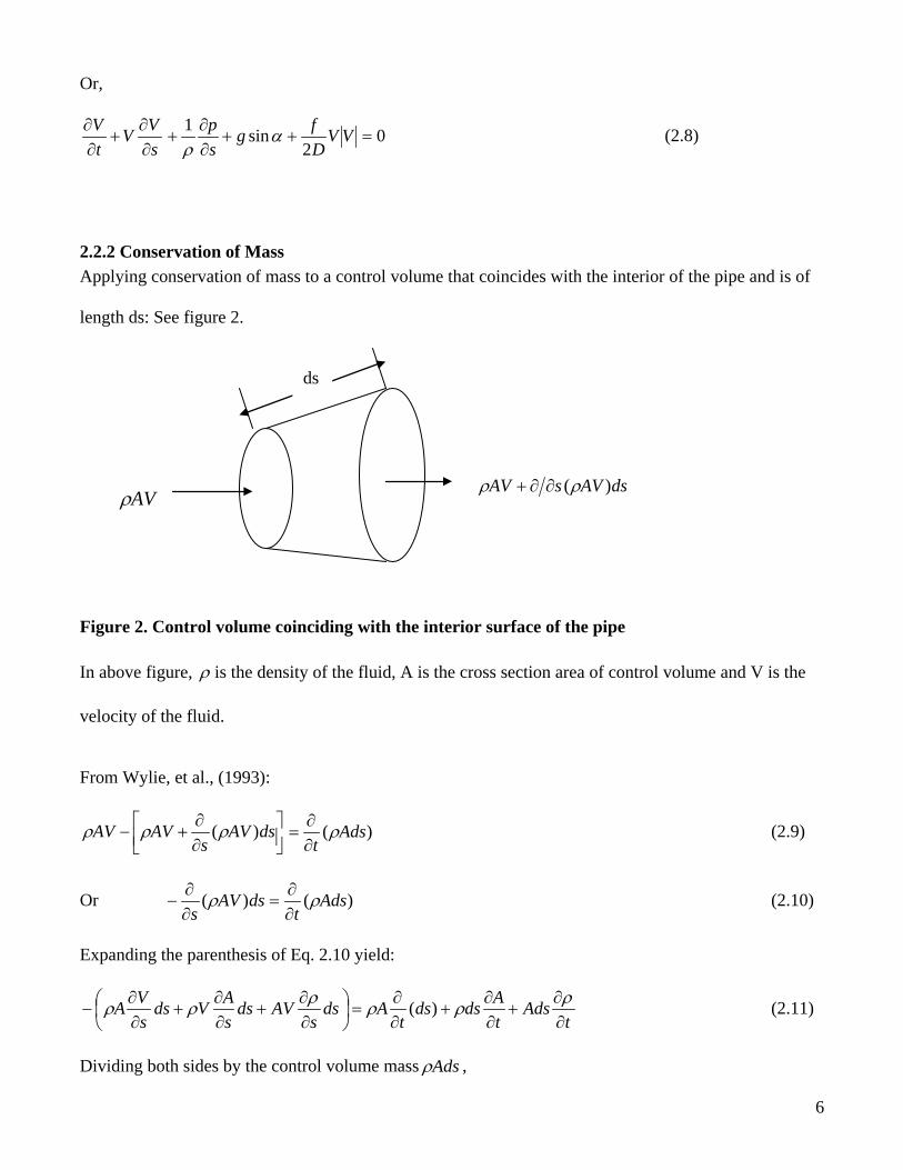
2.2.2 Conservation of Mass Applying conservation of mass to a control volume that coincides with the interior of the pipe and is of
length ds: See figure 2.
Figure 2. Control volume coinciding with the interior surface of the pipe In above figure, ρ is the density of the fluid, A is the cross section area of control volume and V is the
velocity of the fluid.
From Wylie, et al., (1993):
∂∂
+− dsAVs
AVAV )(ρρρ )( Adstρ
∂∂
= (2.9)
Or )()( Adst
dsAVs
ρρ∂∂
=∂∂
− (2.10)
Expanding the parenthesis of Eq. 2.10 yield:
tAds
tAdsds
tAds
sAVds
sAVds
sVA
∂∂
+∂∂
+∂∂
=
∂∂
+∂∂
+∂∂
−ρρρρρρ )( (2.11)
Dividing both sides by the control volume mass Adsρ ,
ds
dsAVsAV )(ρρ ∂∂+ AVρ
7
ttA
Ads
tdssV
sAV
AsV
∂∂
+∂∂
+∂∂
=
∂∂
+∂∂
+∂∂
−ρ
ρρ
ρ11)(111 (2.12)
Regrouping above Eq we get:
0)(111=
∂∂
+∂∂
+
∂∂
+∂∂
+
∂∂
+∂∂
sVds
tdssAV
tA
AsV
tρρ
ρ (2.13)
Recognizing that dtd
sV
tρρρ
=∂∂
+∂∂ and
dtdA
sAV
tA
=∂∂
+∂∂ , Eq. 2.13 becomes
0)(111=
∂∂
+++sVds
dtd
dsdtdA
Adtdρ
ρ (2.14)
^ ^ ^ ^ Terms: T(1) T(2) T(3) T(4)
Let’s split this Eq. 2.14 in various terms as below, we get:
T(1): dtdρ
ρ1
Bulk modulus of elasticity for a liquid (K) is expressed as (Larock et al., 2000):
ρρνν ddp
ddpK =−= , Now T(1) becomes:
dtdp
Kdtd 11
=ρ
ρ (2.15)
T(2): dtdA
A1
The above term can be expressed as (Larock et al., 2000):
dtdp
eED
dtdA
A)1(1 2µ−= (2.16)
Where,
µ = Poisson’s ratio (of the pipe)
e = Pipe wall thickness
E = Young’s Modulus of the pipe
8
T(3): )(1 dsdtd
ds
Considering longitudinal expansion of the pipe (Larock et al., 2000):
dsddsd 1)( ε= (2.17)
Where 1ε is the strain along the pipe axis.
For all the buried pipes, axial movement is restrained. So differential change in strain along pipe axis
( 1εd ) = 0.
Therefore, 0)(1=ds
dtd
ds
Making all these substitutions in Eq. 2.14 yields,
dtdp
K1 +
dtdp
eED)1( 2µ− +
sV∂∂ =0 (2.18)
0)1(1 2 =∂∂
+
−+
sV
eED
Kdtdp µ (2.19)
Wave speed (Larock et al., 2000) can be defined as the time taken by the pressure wave generated by
instantaneous change in velocity to propogate from one point to another in a closed conduit. Wave
speed(c) can be expressed as:
111 22 =
−+
EeD
Kc µρ (2.20)
Hence by using Eq. 2.20 we can write Eq. 2.19 as,
012 =
∂∂
+
sV
cdtdp
ρ (2.21)
02 =∂∂
+sVc
dtdp ρ (2.22)
Or,
spV
tp
∂∂
+∂∂ 02 =
∂∂
+sVc ρ (2.23)
9
2.3 Method of characteristics The significance of method of characteristics is the successful replacement of a pair of partial
differential equations by an equivalent set of ordinary differential equations. The method of
characteristics is developed from assuming that the Eq. 2.9 and Eq. 2.23 can be replaced by a linear
combination of themselves (Wylie, et al.,1993)
02
sin1 2 =∂∂
+∂∂
+∂∂
+
++
∂∂
+∂∂
+∂∂
sVc
spV
tpVV
Dfg
sp
sVV
tV ρα
ρλ (2.24)
Rearranging the terms in above, we have
02
sin2
=
++
∂∂
++
∂∂
+
∂∂
++
∂∂ VV
Dfg
spV
tp
sVcV
tV αλ
ρλ
λρλ (2.25)
Assuming,
ρλ
λρ
+=+= VcVdtds 2
(2.26)
The equality in Eq. 2.26 leads to
ρλ c±= (2.27)
Which when substituted back into Eq. 2.26 leads to
cVdtds
±= (2.28)
Use of proper positive and negative signs of lambda permits writing of the following sets of ordinary
differential equations (Wylie, et al.,1993):
+=
=++++
cVdtds
DVfV
gdtdp
cdtdV
C0
2sin1 α
ρ (2.29)
and
10
−=
=++−−
cVdtds
DVfV
gdtdp
cdtdV
C0
2sin1 α
ρ (2.30)
Finally we replace the pressure in favor of total head using (Wylie, et al.,1993) )( zHp −= γ and we
assume that the entire pipe network is in the same horizontal plane. i.e., 0sin =α .
The new set of characteristic equations can be written as (Wylie, et al.,1993)
02
: =+++
DVfV
dtdH
cg
dtdVC Only when cV
dtds
+= (2.31)
02
: =+−−
DVfV
dtdH
cg
dtdVC Only when cV
dtds
−= (2.32)
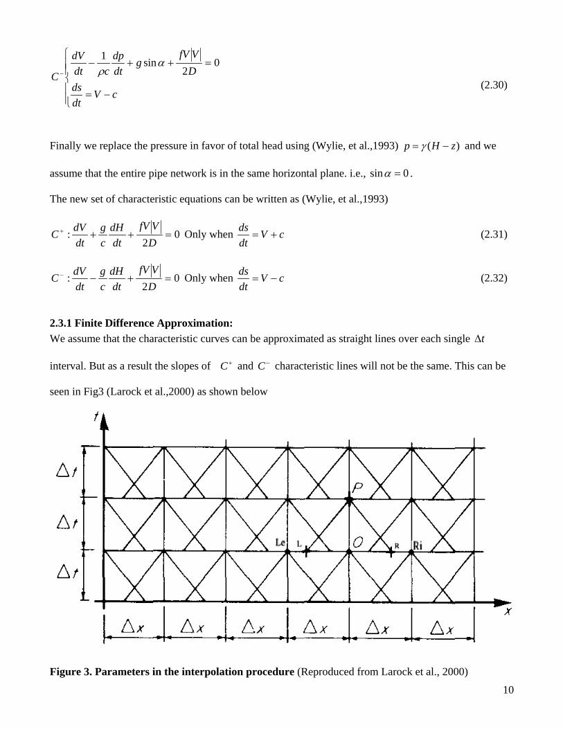
2.3.1 Finite Difference Approximation: We assume that the characteristic curves can be approximated as straight lines over each single t∆
interval. But as a result the slopes of +C and −C characteristic lines will not be the same. This can be
seen in Fig3 (Larock et al.,2000) as shown below
Figure 3. Parameters in the interpolation procedure (Reproduced from Larock et al., 2000)
11
We can see that the characteristics intersecting at P no longer pass through the grid points Le and Ri. But
instead they pass through the points L and R somewhere between Le and Ri .
(2.33)
Hence, the finite difference
approximations to Eqs. 2.31 and 2.32 become
(2.34)
This results in 4 new unknowns RLL VHV ,, and RH . But we overcome this problem by choosing t∆ so
that the point L is near Le and R is near Ri..
+C
Now linear interpolation becomes an accurate way to
evaluate the values of H and V at points L and R.
Along characteristic (Larock et al., 2000),
CLe
CL
CLe
CL
HHHH
VVVV
sx
−−
=−−
=∆∆ (2.35)
with
1
LVctx +=
∆∆ (2.36)
Solving above two equations for LV and LH yields,
CcLeL VsxVVV +
∆∆
−= )( and ccLeL HsxHHH +
∆∆
−= )( (2.37)
Replacing x∆ in these equations using the same relation for tx∆∆ now produces (Larock et al., 2000)
)(1
)(
cLe
cLeC
L
VVst
VVstcV
V−
∆∆
−
−∆∆
+= (2.38)
and
02
02
=+∆−
−∆−
=+∆−
+∆−
RRRPRP
LLLPLP
VVDf
tHH
cg
tVV
VVDf
tHH
cg
tVV
12
))(( LCLeCL VcHHstHH +−
∆∆
+= (2.39)
Similarly along the −C characteristic (Larock et al., 2000),
)(1
)(
cRi
cRiC
R
VVst
VVstcV
V−
∆∆
−
−∆∆
+= (2.40)
And
))(( RCRiCR VcHHstHH −−
∆∆
+= (2.41)
Note that )( cLe VVst
−∆∆ is on the order of
VcV+
, which is very small compared to 1, hence the second
terms in the denominator of Eqs. 2.38 and 2.40 can be neglected. This would result in
)( cLeCL VVstcVV −
∆∆
+= (2.42)
and
)( cRiCR VVstcVV −
∆∆
+= (2.43)
As we now have the known values for RLL VHV ,, and RH ,we can solve the Eqs. 2.33 and 2.34
simultaneously for velocity and head at point P.
The solutions are (Larock et al., 2000):
+
∆−−++= )(
2)()(
21
RRLLRLRLP VVVVDtfHH
cgVVV (2.44)
−
∆−++−= )(
2)()(
21
RRLLRLRLP VVVVDtf
gcHHVV
gcH (2.45)
2.4. Summary of Equations The two basic equations of fluid flow in closed conduits are a pair of quasilinear partial differential
equations (Wylie et al., 1993):
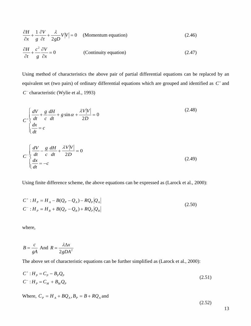
13
02
1=+
∂∂
+∂∂ VV
gDtV
gxH λ (Momentum equation) (2.46)
02
=∂∂
+∂∂
xV
gc
tH (Continuity equation) (2.47)
Using method of characteristics the above pair of partial differential equations can be replaced by an
equivalent set (two pairs) of ordinary differential equations which are grouped and identified as +C and −C characteristic (Wylie et al., 1993)
(2.48)
−=
=+−−
cdtdx
DVV
dtdH
cg
dtdV
C0
2λ
(2.49)
Using finite difference scheme, the above equations can be expressed as (Larock et al., 2000):
BPBPBP
APAPAP
QRQQQBHHC
QRQQQBHHC
+−+=
−−−=−
+
)(:
)(: (2.50)
where,
gAcB = And 22gDA
xR ∆=
λ
The above set of characteristic equations can be further simplified as (Larock et al., 2000):
PMMP
PPPP
QBCHCQBCHC
+=
−=−
+
:
: (2.51)
Where, APAAP RQBBBQHC +=+= , and (2.52)
=
=++++
cdtdx
DVV
gdt
dHcg
dtdV
C0
2sin
λα
14
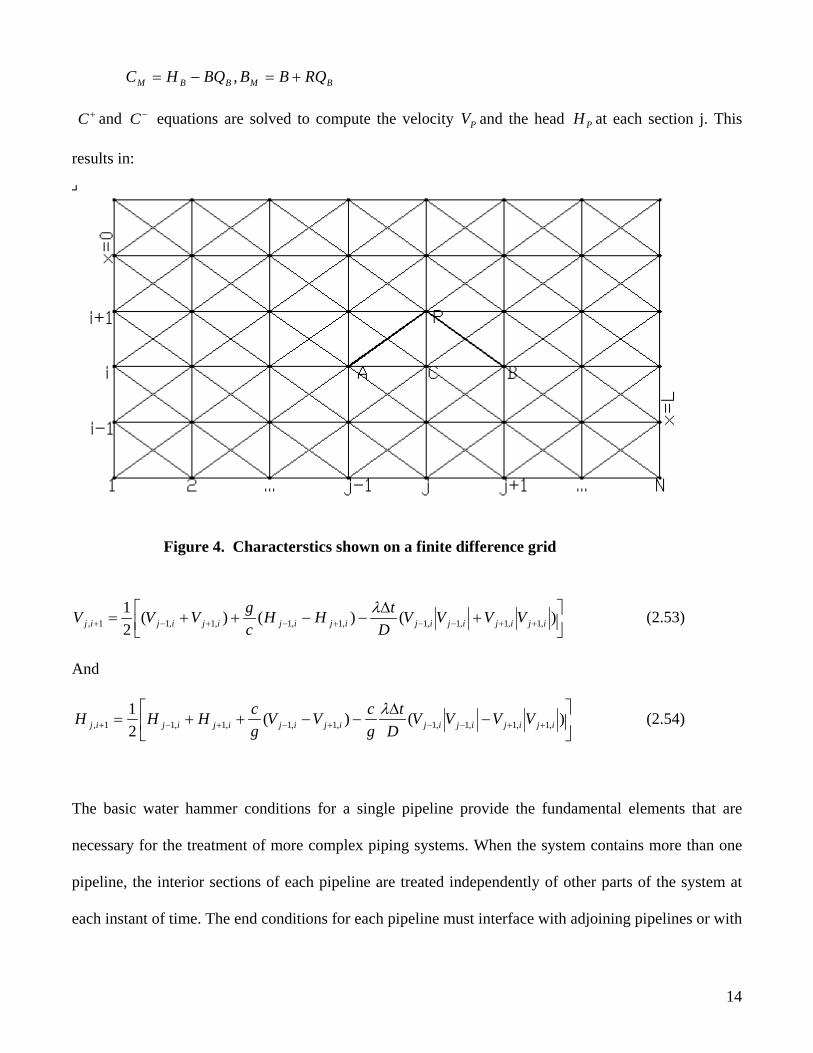
BMBBM RQBBBQHC +=−= , +C and −C equations are solved to compute the velocity PV and the head PH at each section j. This
results in:
Figure 4. Characterstics shown on a finite difference grid
+
∆−−++= ++−−+−+−+ )()()(
21
,1,1,1,1,1,1,1,11, ijijijijijijijijij VVVVD
tHHcgVVV λ (2.53)
And
−
∆−−++= ++−−+−+−+ )()(
21
,1,1,1,1,1,1,1,11, ijijijijijijijijij VVVVD
tgcVV
gcHHH λ (2.54)
The basic water hammer conditions for a single pipeline provide the fundamental elements that are
necessary for the treatment of more complex piping systems. When the system contains more than one
pipeline, the interior sections of each pipeline are treated independently of other parts of the system at
each instant of time. The end conditions for each pipeline must interface with adjoining pipelines or with
15
other boundary elements. Again each boundary condition is treated independently of other parts of the
system.
2.5 Boundary Conditions Analyzing the following boundary conditions is important part of water hammer study:
2.5.1 Reservoir
Consider a single pipe system with reservoir at the upstream of the pipe. Hence, a −C characteristic can
be drawn from a node closest to the reservoir towards the junction. Therefore from Eq. 2.51:
PMMP QBCHC +=− : (2.55)
Here, PH is the head at the reservoir junction and is assumed constant.
Hence, RP HH = and discharge at this junction can be obtained as:
M
MRP B
CHQ −= (2.56)
2.5.2 Valve Consider a single pipe system with reservoir upstream and valve at downstream. From the node closest
to the valve and towards its left, a +C characteristic can be drawn towards the valve junction. Therefore
from Eq. 2.51
PPPP QBCHC −=+ : . (2.57)
During steady state flow through the valve, orifice equation can be applied as (Watters, 1984):
PvdP gHACQ 2)(= (2.58) Solving above two equations, we obtain
16
2222 )(2))(()( vdPvdPvdPP ACgCACgBACgBQ ++−= (2.59)
2.5.3 Pumps and Turbines Pump/Turbine characteristic curves are needed for finding the water hammer caused by them. Let SH be
the head at suction side of the pump. Let DH be the head at discharge side of the pump. The difference
in head ( DH - SH ) gives the total head ( PH ) developed by the pump.
),( PP QnfH = (2.60)
The above equation (Chaudhry, 1988) is a typical form of pump/turbine characteristic curve. Where, n is
the pump speed and PQ is the pump discharge.
Also in this case, the characteristic equations are:
PMMD
PPPS
QBCHCQBCHC
+=
−=−
+
:
: (2.61)
Solving above three basic equations, we obtain discharge and head at the pump during transients.
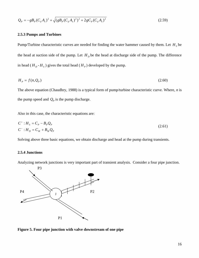
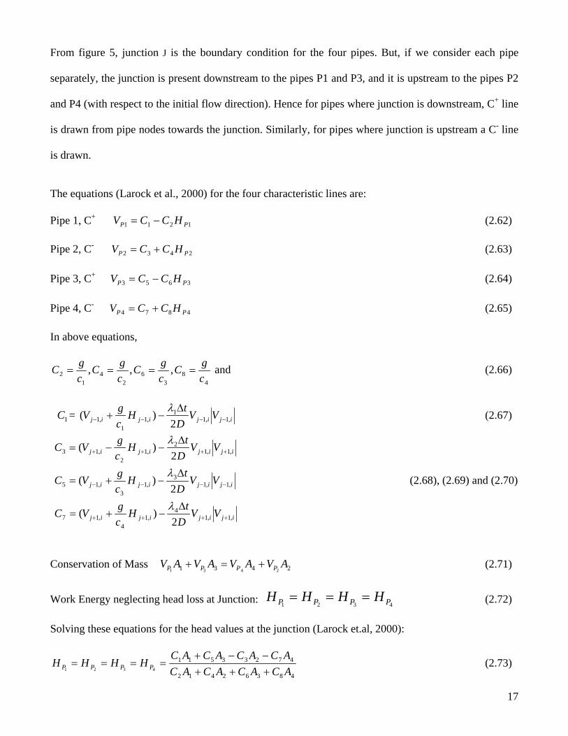
2.5.4 Junctions Analyzing network junctions is very important part of transient analysis. Consider a four pipe junction.
Figure 5. Four pipe junction with valve downstream of one pipe
P1
P2
P3
P4 J
17
From figure 5, junction J is the boundary condition for the four pipes. But, if we consider each pipe
separately, the junction is present downstream to the pipes P1 and P3, and it is upstream to the pipes P2
and P4 (with respect to the initial flow direction). Hence for pipes where junction is downstream, C+ line
is drawn from pipe nodes towards the junction. Similarly, for pipes where junction is upstream a C- line
is drawn.
The equations (Larock et al., 2000) for the four characteristic lines are: Pipe 1, C+
1211 PP HCCV −= (2.62) Pipe 2, C-
2432 PP HCCV += (2.63) Pipe 3, C+
3653 PP HCCV −= (2.64) Pipe 4, C-
4874 PP HCCV += (2.65) In above equations,
48
36
24
12 ,,,
cgC
cgC
cgC
cgC ==== and (2.66)
1C = ijijijij VVD
tHcgV ,1,1
1,1
1,1 2
)( −−−−
∆−+λ
(2.67)
ijijijij
ijijijij
ijijijij
VVD
tHcgVC
VVD
tH
cgVC
VVD
tHcgVC
,1,14
,14
,17
,1,13
,13
,15
,1,12
,12
,13
2)(
2)(
2)(
++++
−−−−
++++
∆−+=
∆−+=
∆−−=
λ
λ
λ
(2.68), (2.69) and (2.70)
Conservation of Mass 2431 2431
AVAVAVAV PPPP +=+ (2.71)
Work Energy neglecting head loss at Junction: 4321 PPPP HHHH === (2.72)
Solving these equations for the head values at the junction (Larock et.al, 2000):
48362412
472335114321 ACACACAC
ACACACACHHHH PPPP +++
−−+==== (2.73)
18
Back substitution of these heads into Eqs. 2.62, 2.63, 2.64 and 2.65 yields the velocities in each of the
pipes.
Consider a distribution network which is in steady state. Let the valve at the downstream of pipe2 be
closed suddenly (as shown in Fig 5) at time t = 0 sec. Each pipe connected to the junction is divided
into N number of sections. A rectangular grid can be drawn showing N sections each of length s∆ on x-
axis and t∆ increments on y-axis. At each t∆ time step increments head and discharge at each node are
calculated using method of characteristics (finite difference approximation).
At the node closest to the valve at upstream end of pipe 2, head and discharge are calculated using valve
boundary conditions and at the node closest to the junction, boundary conditions of the junction are used
to evaluate head and discharge.
Now consider pipe3, which is an inflow pipe to the Junction:
At the node (of pipe 3) closest to the junction, a negative characteristic from the junction and positive
characteristic from the left adjacent node are drawn to meet at the first time step. And subsequently head
and discharge are evaluated. So, is the case with all other pipes attached to the junction.
2.6 Transient Flow Analysis
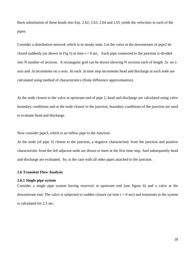
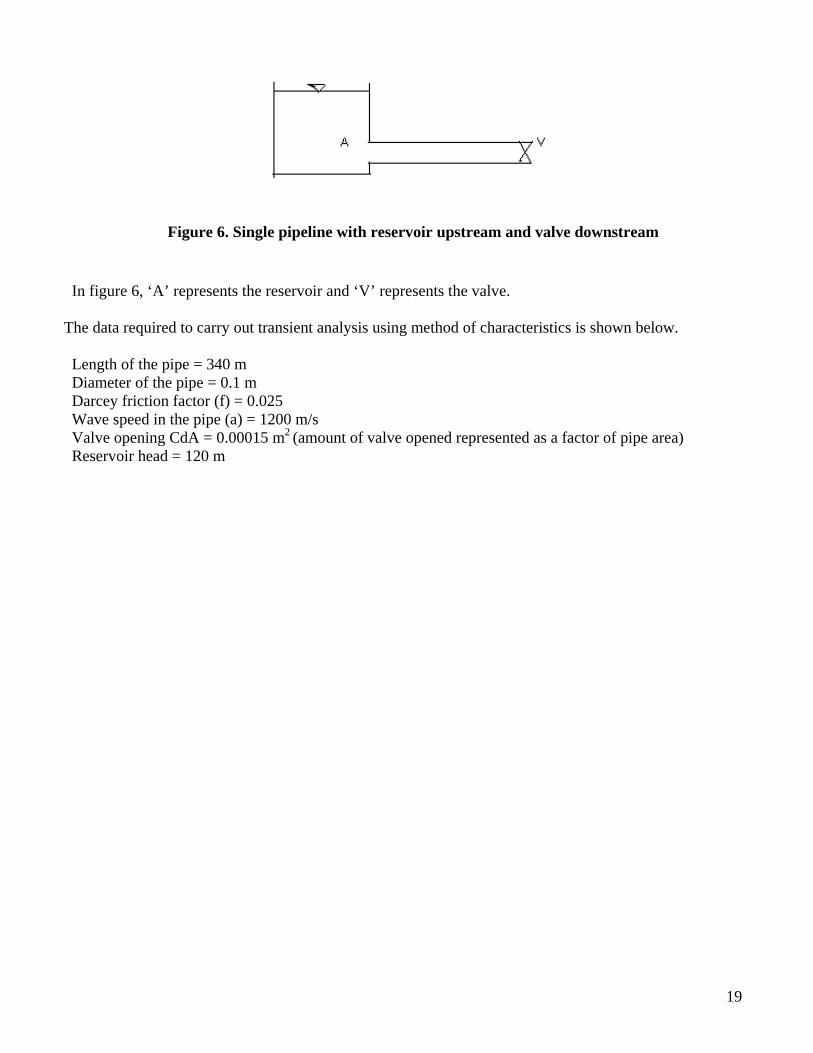
2.6.1 Single pipe system Consider a single pipe system having reservoir at upstream end (see figure 6) and a valve at the
downstream end. The valve is subjected to sudden closure (at time t = 0 sec) and transients in the system
is calculated for 2.5 sec.
19
Figure 6. Single pipeline with reservoir upstream and valve downstream
In figure 6, ‘A’ represents the reservoir and ‘V’ represents the valve.
The data required to carry out transient analysis using method of characteristics is shown below.
Length of the pipe = 340 m Diameter of the pipe = 0.1 m Darcey friction factor (f) = 0.025 Wave speed in the pipe (a) = 1200 m/s Valve opening CdA = 0.00015 m2
(amount of valve opened represented as a factor of pipe area) Reservoir head = 120 m
20
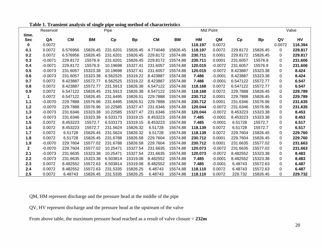
Table 1. Transient analysis of single pipe using method of characteristics Reservoir Pipe Mid Point Valve
time. Sec QA CM BM Cp Bp CM BM HM QM Cp Bp QV HV
0 0.0072
118.197 0.0072
0.0072 116.394 0.1 0.0072 6.576956 15826.45 231.6201 15826.45 4.774048 15826.45 118.197 0.0072 229.8172 15826.45 0 229.817 0.2 0.0072 6.576956 15826.45 231.6201 15826.45 229.8172 15574.88 230.711 0.0001 229.8172 15826.45 0 229.817 0.3 -0.0071 229.8172 15576.9 231.6201 15826.45 229.8172 15574.88 230.711 0.0001 231.6057 15576.9 0 231.606 0.4 -0.0071 229.8172 15576.9 10.19698 15327.41 231.6057 15574.88 120.015 -0.0072 231.6057 15576.9 0 231.606 0.5 -0.0073 231.6057 15323.38 10.19698 15327.41 231.6057 15574.88 120.015 -0.0072 8.423887 15323.38 0 8.424 0.6 -0.0073 231.6057 15323.38 6.562525 15319.22 8.423887 15574.88 7.486 -0.0001 8.423887 15323.38 0 8.424 0.7 0.0072 8.423887 15572.77 6.562525 15319.22 8.423887 15574.88 7.486 -0.0001 6.547122 15572.77 0 6.547 0.8 0.0072 8.423887 15572.77 231.5913 15826.38 6.547122 15574.88 118.168 0.0072 6.547122 15572.77 0 6.547 0.9 0.0072 6.547122 15826.45 231.5913 15826.38 6.547122 15574.88 118.168 0.0072 229.7888 15826.45 0 229.789 1 0.0072 6.547122 15826.45 231.6495 15826.51 229.7888 15574.88 230.712 0.0001 229.7888 15826.45 0 229.789
1.1 -0.0070 229.7888 15576.96 231.6495 15826.51 229.7888 15574.88 230.712 0.0001 231.6346 15576.96 0 231.635 1.2 -0.0070 229.7888 15576.96 10.22585 15327.47 231.6346 15574.88 120.044 -0.0072 231.6346 15576.96 0 231.635 1.3 -0.0073 231.6346 15323.38 10.22585 15327.47 231.6346 15574.88 120.044 -0.0072 8.453223 15323.38 0 8.453 1.4 -0.0073 231.6346 15323.38 6.533173 15319.15 8.453223 15574.88 7.485 -0.0001 8.453223 15323.38 0 8.453 1.5 0.0072 8.453223 15572.7 6.533173 15319.15 8.453223 15574.88 7.485 -0.0001 6.51728 15572.7 0 6.517 1.6 0.0072 8.453223 15572.7 231.5624 15826.32 6.51728 15574.88 118.139 0.0072 6.51728 15572.7 0 6.517 1.7 0.0072 6.51728 15826.45 231.5624 15826.32 6.51728 15574.88 118.139 0.0072 229.7604 15826.45 0 229.760 1.8 0.0072 6.51728 15826.45 231.6788 15826.58 229.7604 15574.88 230.712 0.0001 229.7604 15826.45 0 229.760 1.9 -0.0070 229.7604 15577.02 231.6788 15826.58 229.7604 15574.88 230.712 0.0001 231.6635 15577.02 0 231.663 2 -0.0070 229.7604 15577.02 10.25471 15327.54 231.6635 15574.88 120.073 -0.0072 231.6635 15577.02 0 231.663
2.1 -0.0073 231.6635 15323.38 10.25471 15327.54 231.6635 15574.88 120.073 -0.0072 8.482552 15323.38 0 8.483 2.2 -0.0073 231.6635 15323.38 6.503814 15319.08 8.482552 15574.88 7.485 -0.0001 8.482552 15323.38 0 8.483 2.3 0.0072 8.482552 15572.63 6.503814 15319.08 8.482552 15574.88 7.485 -0.0001 6.48743 15572.63 0 6.487 2.4 0.0072 8.482552 15572.63 231.5335 15826.25 6.48743 15574.88 118.110 0.0072 6.48743 15572.63 0 6.487 2.5 0.0072 6.48743 15826.45 231.5335 15826.25 6.48743 15574.88 118.110 0.0072 229.732 15826.45 0 229.732
QM, HM represent discharge and the pressure head at the middle of the pipe
QV, HV represent discharge and the pressure head at the upstream of the valve
From above table, the maximum pressure head reached as a result of valve closure = 232m
21
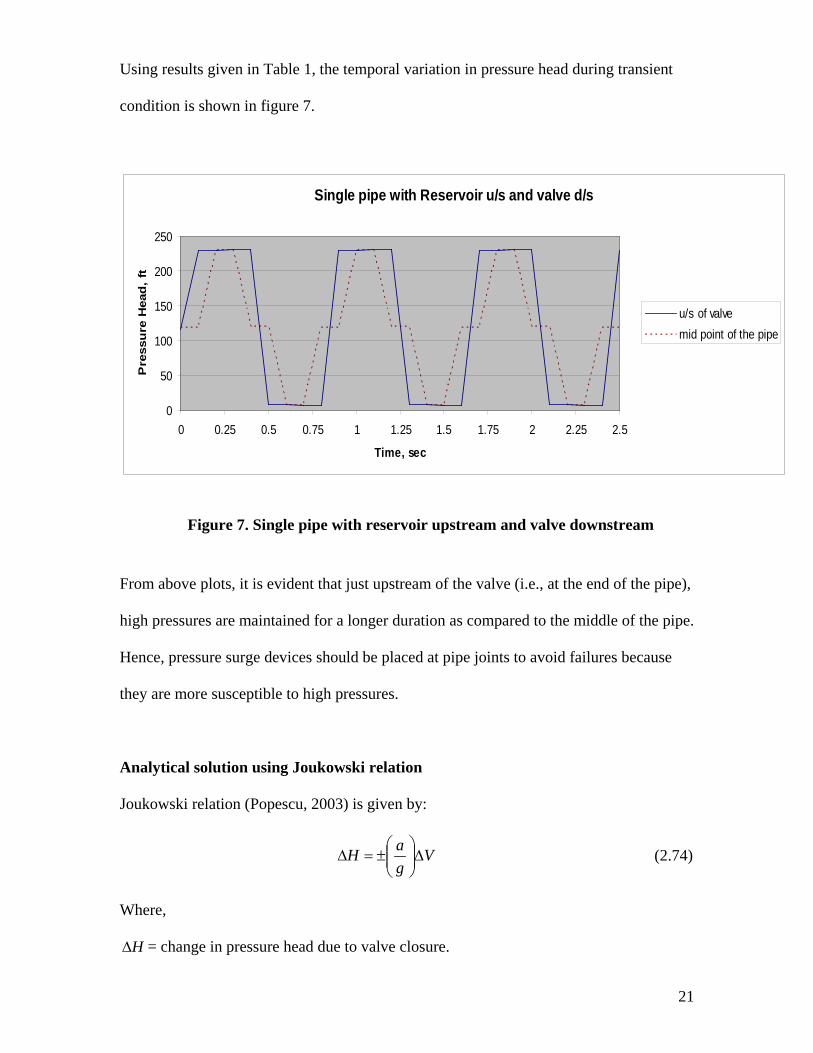
Using results given in Table 1, the temporal variation in pressure head during transient
condition is shown in figure 7.
Single pipe with Reservoir u/s and valve d/s
0
50
100
150
200
250
0 0.25 0.5 0.75 1 1.25 1.5 1.75 2 2.25 2.5
Time, sec
Pre
ssu
re H
ead
, ft
u/s of valvemid point of the pipe
Figure 7. Single pipe with reservoir upstream and valve downstream
From above plots, it is evident that just upstream of the valve (i.e., at the end of the pipe),
high pressures are maintained for a longer duration as compared to the middle of the pipe.
Hence, pressure surge devices should be placed at pipe joints to avoid failures because
they are more susceptible to high pressures.
Analytical solution using Joukowski relation
Joukowski relation (Popescu, 2003) is given by:
VgaH ∆
±=∆ (2.74)
Where,
H∆ = change in pressure head due to valve closure.
22
a = Wave speed in the pipe.
g = acceleration due to gravity = 9.8 m/s^2
V∆ = change in fluid velocity = 0.91 m/s
Using the same example problem as above, we can find the change in pressure head due
to sudden valve closure using Joukowski relation as:
9.0806.9
1200
±=∆H 1= 111.4 m
Steady state pressure head at the valve = Head in the Reservoir = 120 m (neglecting
friction losses in the pipe)
Hence, maximum pressure head at the valve = 111.4 m + 120 m = 231 m
Results
The maximum pressure head at the valve from method of characteristics = 232 m
The maximum pressure head at the valve from Joukowski relation = 231 m
The values obtained from both these analysis are very close. This can be explained by the
simplicity of the pipe system we have chosen (single pipe with reservoir at upstream end
and valve at downstream end). Simple expressions, such as the Joukowski relation are
only applicable under restricted circumstances. The two most important restrictions are:
1) There should be no head loss resulting from friction.
2) There should be no wave reflections (i.e., there is no interaction between devices
or boundary conditions in the system).
The above restrictions are narrowly met by the single pipe system discussed above.
Hence, the results are comparable.
23
In above section, transient analysis in a single pipe system is solved using method of
characteristics and found that the resulting maximum pressure head value and that
obtained by Joukowski relation gave close results.
Most of the times, transient analysis performed on single pipe sytem is useful only for
experimental purposes. In practice, most of the distribution systems have multiple pipes
and transient flow analysis plays a significant role at pipe joints and at locations where
pressure control devices such as valves and pumps exist.
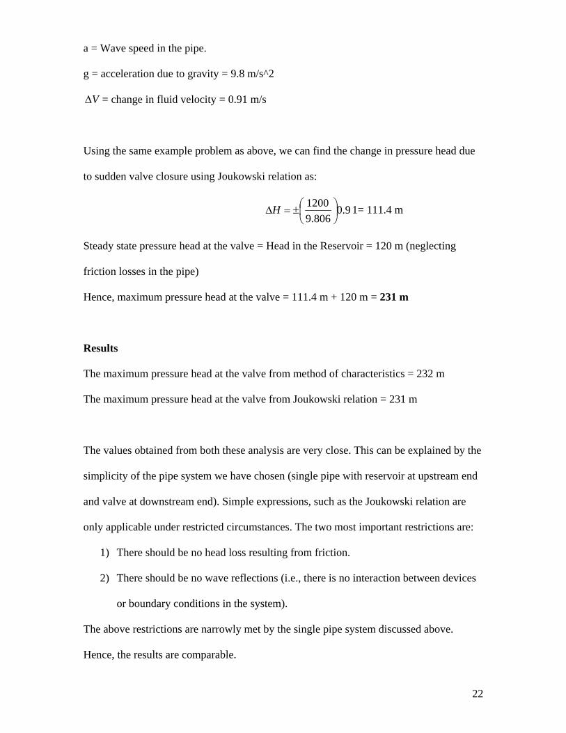
2.6.2 Network Distribution Consider the network given below (Larock et al., 2000). The Hazen-Williams roughness
coefficient is 120 for all pipes. This network experiences a transient that is caused by the
sudden closure of a valve at the downstream end of pipe 5. Wave speed is 2850 ft/s for all
the pipes. Transient analysis is obtained for this network.
Figure 8. Network distribution system
The pipe information is given in Table 2.
Table 2. Pipe data Pipe Length(ft) Diameter(in) 1 3300 12 2 8200 8 3 3300 8 4 4900 12 5 3300 6 6 2600 14
P
4200 ft 4130 ft
(1)
(2)
(3) (4)
(5)
(6) 1 2
3
4
5
6
4130 ft
P: Pump X: Valve
24
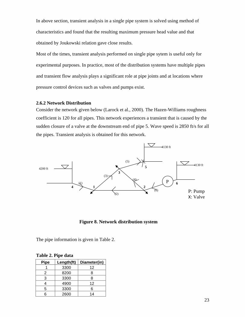
The node information is given in Table 3.
Table 3. Node data Node Elevation(ft) Demand(gal/min)
1 3800 475 2 3830 317 3 3370 790 4 4050 5 4000 6 4010
Steady state analysis:
First, the above network distribution system is solved for steady state analysis.Following
this, transient analysis is performed. A program called “NETWK” was adopted for steady
state analysis of above network. “NETWK” is a FORTRAN 95 code (Larock et al., 2000)
which can perform steady state analysis on complex pipe systems. The results are shown
in Table 4.
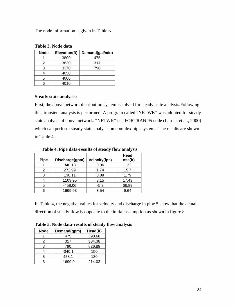
Table 4. Pipe data-results of steady flow analysis
Pipe Discharge(gpm) Velocity(fps) Head
Loss(ft) 1 340.13 0.96 1.32 2 272.99 1.74 15.7 3 138.11 0.88 1.79 4 1109.95 3.15 17.49 5 -458.06 -5.2 66.89 6 1699.93 3.54 9.64
In Table 4, the negative values for velocity and discharge in pipe 5 show that the actual
direction of steady flow is opposite to the initial assumption as shown in figure 8.
Table 5. Node data-results of steady flow analysis Node Demand(gpm) Head(ft)
1 475 398.68 2 317 384.38 3 790 826.89 4 -340.1 150 5 458.1 130 6 -1699.9 214.03
25
In Table 5, the negative values for demand indicate that the flow direction is into the
node. Detailed steady state flow output obtained from “NETWK” program is shown in
Appendix A-1. This output is used as one of the input files for the transient analysis.
Transient Analysis:
In order to perform transient analysis, “TRANSNET” program is adopted.
“TRANSNET” is the FORTRAN 95 code (Larock et al., 2000) which can perform
transient analysis caused by sudden valve closures or pump failures. In pipe network
shown in figure 8, the valve located on pipe 5 is closed suddenly at time 0.0 s and below
is the summary of results for pipe 5 at time 7.73 s when column separation occurs.
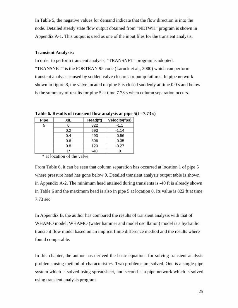
Table 6. Results of transient flow analysis at pipe 5(t =7.73 s) Pipe X/L Head(ft) Velocity(fps)
5 0 822 -1.1 0.2 693 -1.14 0.4 493 -0.56 0.6 306 -0.35 0.8 120 -0.27 1* -40 0
* at location of the valve
From Table 6, it can be seen that column separation has occurred at location 1 of pipe 5
where pressure head has gone below 0. Detailed transient analysis output table is shown
in Appendix A-2. The minimum head attained during transients is -40 ft is already shown
in Table 6 and the maximum head is also in pipe 5 at location 0. Its value is 822 ft at time
7.73 sec.
In Appendix B, the author has compared the results of transient analysis with that of
WHAMO model. WHAMO (water hammer and model oscillation) model is a hydraulic
transient flow model based on an implicit finite difference method and the results where
found comparable.
In this chapter, the author has derived the basic equations for solving transient analysis
problems using method of characteristics. Two problems are solved. One is a single pipe
system which is solved using spreadsheet, and second is a pipe network which is solved
using transient analysis program.
26
In literature most of the transients programs are in FORTRAN language. In chapter 3, the
author used Java to code transient analysis program using an object oriented approach.
The results of Java program are compared with that obtained from “TRANSNET”
program.
27
CHAPTER 3: An Object Oriented Approach for Transient Analysis in Water Distribution Systems using JAVA programming
3.1 Introduction
Most of the algorithms in computational hydraulics discipline are written in procedural
language (FORTRAN, Pascal and C). Procedural programming was found to be adequate for
coding moderately extensive programs until 90’s (Madan, 2004). In procedural programming,
the strategy is based on dividing the computational task into smaller groups termed as
functions, procedures or subroutines which perform well-defined operations on their input
arguments and have well defined interfaces to other subprograms in the main program.
However, procedural programming approach can get challenging when the code needs to be
extended for enhancing the scope of the ptogram. A detailed knowledge of the program is
required to work on a small part of the code and poor equivalence between program variables
and physical entities further makes it difficult. Integrity of data is another area of concern in
procedural programs because, the emphasis is on functions and data is considered secondary.
All the functions of a program have access to data and as a result data is highly susceptible to
get corrupted when dealing with complex programs. In addition, there are difficulties related to
reusability and maintenance of code as procedural programs are platform and version
dependent.
Object oriented programming is developed with the objective of addressing some of the typical
difficulties associated with procedural programming approach (Madan, 2004). The concept of
Object-oriented programming (OOP) began in 1970s and found its first convivial
concretization with the Small Talk (Fenves, 1992) language at the beginning of the eighties.
Object oriented applications in scientific computing appeared around 1990 and since then its
use has been spreading.
Madan (2004) discussed the modeling and design of structural analysis programs using OOP
approach. He developed a C++ program for matrix analysis of a space frame. Krishnamoorthy
et al., (2002) used object oriented approach to design and develop a genetic algorithm library
28
for solving optimization problems. They later solved a space truss optimization problem by
implementing this library. A window-based finite-element analysis program was developed by
Ju and Hosain (1996). Graphical finite element objects developed using C++ language were
implemented in the program.
Liu et al., (2003) developed an object oriented framework for structural analysis and design.
They implemented this framework in optimal design of energy dissipation device (EDD)
configurations for best structural performance under earthquake conditions. Tisdale (1996)
followed object oriented approach to organize South Florida hydrologic system information as
object, dynamic and functional modules. These modules can be used for hydrologic software
development.
A real-time flood forecasting system called RIBS (Real time Interactive Basin Simulator) is
developed by Garrote and Becchi (1997) using object-oriented framework. Primary
applications of RIBS include rainfall forecasting, estimate runoff generating potential of
watersheds, and to develop hydrographs. Solomatine (1996) presented a water distribution
modeling system (HIS) as an example of object oriented design. He developed two models
namely, LinHIS – to solve for linear system of pipes, and NetHIS – to solve for a distributed
network of pipes. In both cases, flow is considered either steady or quasi-steady.
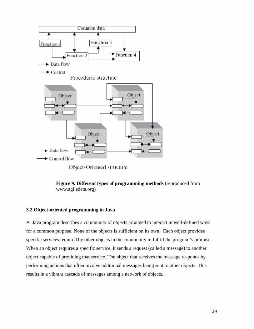
Figure 9 depicts the basic difference between the organization of an object –oriented program
and a procedure-oriented program. In procedure-oriented program, there are different
functions, each of which perform specific action by accessing the data common to all functions
whereas in object-oriented program, each object has its own data and methods.
29
Figure 9. Different types of programming methods (reproduced from www.agiledata.org)
3.2 Object-oriented programming in Java A Java program describes a community of objects arranged to interact in well-defined ways
for a common purpose. None of the objects is sufficient on its own. Each object provides
specific services required by other objects in the community to fulfill the program’s promise.
When an object requires a specific service, it sends a request (called a message) to another
object capable of providing that service. The object that receives the message responds by
performing actions that often involve additional messages being sent to other objects. This
results in a vibrant cascade of messages among a network of objects.
30
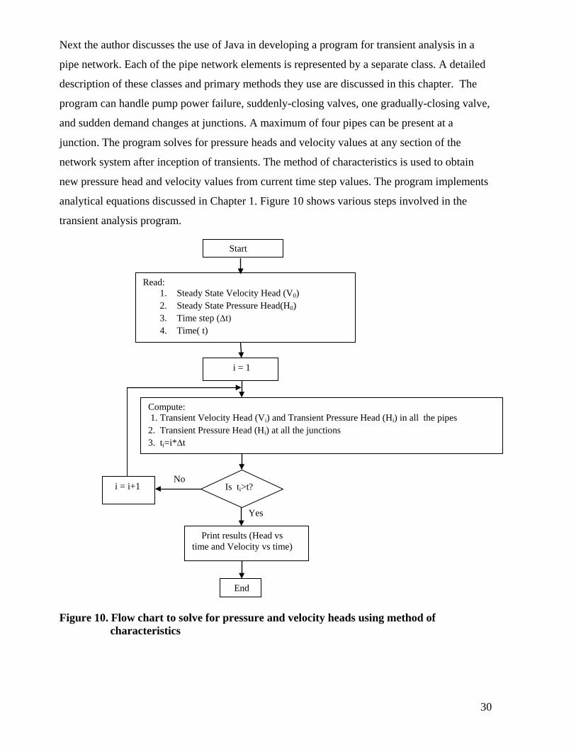
Next the author discusses the use of Java in developing a program for transient analysis in a
pipe network. Each of the pipe network elements is represented by a separate class. A detailed
description of these classes and primary methods they use are discussed in this chapter. The
program can handle pump power failure, suddenly-closing valves, one gradually-closing valve,
and sudden demand changes at junctions. A maximum of four pipes can be present at a
junction. The program solves for pressure heads and velocity values at any section of the
network system after inception of transients. The method of characteristics is used to obtain
new pressure head and velocity values from current time step values. The program implements
analytical equations discussed in Chapter 1. Figure 10 shows various steps involved in the
transient analysis program.
Figure 10. Flow chart to solve for pressure and velocity heads using method of characteristics
Start
Read: 1. Steady State Velocity Head (V0) 2. Steady State Pressure Head(H0) 3. Time step (∆t) 4. Time( t)
i = 1
Compute: 1. Transient Velocity Head (Vi) and Transient Pressure Head (Hi) in all the pipes 2. Transient Pressure Head (Hi) at all the junctions 3. ti=i*∆t
Is ti>t?
i = i+1
Yes
Print results (Head vs time and Velocity vs time)
No
End
31
The pipe network problem discussed in Section 2.6.2 in Chapter 2 is solved using Java
program and results are compared with TRANSNET program output are discussed next.
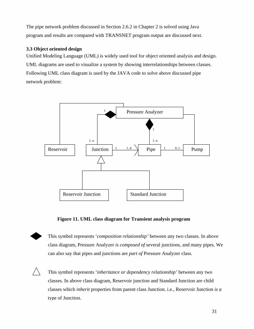
3.3 Object oriented design Unified Modeling Language (UML) is widely used tool for object oriented analysis and design.
UML diagrams are used to visualize a system by showing interrelationships between classes.
Following UML class diagram is used by the JAVA code to solve above discussed pipe
network problem:
Figure 11. UML class diagram for Transient analysis program
Pressure Analyzer
Pipe Junction Pump Reservoir
Reservoir Junction Standard Junction
1 1..4
1
1..n
1
1..n
1 0..1
This symbol represents ‘composition relationship’ between any two classes. In above
class diagram, Pressure Analyzer is composed of several junctions, and many pipes. We
can also say that pipes and junctions are part of Pressure Analyzer class.
This symbol represents ‘inheritance or dependency relationship’ between any two
classes. In above class diagram, Reservoir junction and Standard Junction are child
classes which inherit properties from parent class Junction. i.e., Reservoir Junction is a
type of Junction.
32
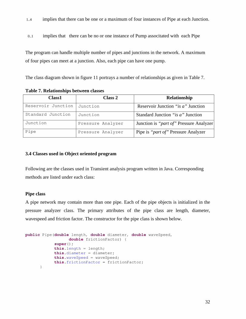
1..4 implies that there can be one or a maximum of four instances of Pipe at each Junction.
0..1 implies that there can be no or one instance of Pump associtated with each Pipe
The program can handle multiple number of pipes and junctions in the network. A maximum
of four pipes can meet at a junction. Also, each pipe can have one pump.
The class diagram shown in figure 11 portrays a number of relationships as given in Table 7.
Table 7. Relationships between classes Class1 Class 2 Relationship
Reservoir Junction Junction Reservoir Junction “is a” Junction Standard Junction Junction Standard Junction “is a” Junction Junction Pressure Analyzer Junction is “part of” Pressure Analyzer Pipe Pressure Analyzer Pipe is “part of” Pressure Analyzer
3.4 Classes used in Object oriented program
Following are the classes used in Transient analysis program written in Java. Corresponding
methods are listed under each class:
Pipe class
A pipe network may contain more than one pipe. Each of the pipe objects is initialized in the
pressure analyzer class. The primary attributes of the pipe class are length, diameter,
wavespeed and friction factor. The constructor for the pipe class is shown below.
public Pipe(double length, double diameter, double waveSpeed, double frictionFactor) { super(); this.length = length; this.diameter = diameter; this.waveSpeed = waveSpeed; this.frictionFactor = frictionFactor; }
33
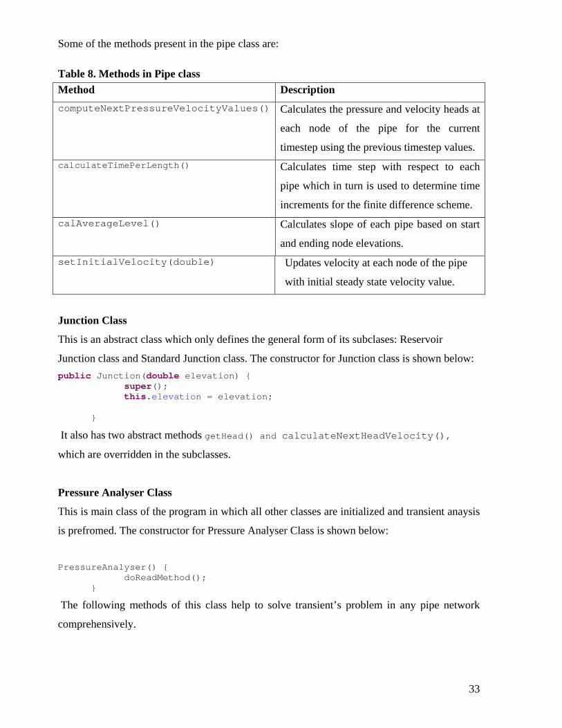
Some of the methods present in the pipe class are:
Table 8. Methods in Pipe class Method Description computeNextPressureVelocityValues() Calculates the pressure and velocity heads at
each node of the pipe for the current
timestep using the previous timestep values. calculateTimePerLength() Calculates time step with respect to each
pipe which in turn is used to determine time
increments for the finite difference scheme. calAverageLevel() Calculates slope of each pipe based on start
and ending node elevations. setInitialVelocity(double) Updates velocity at each node of the pipe
with initial steady state velocity value.
Junction Class
This is an abstract class which only defines the general form of its subclases: Reservoir
Junction class and Standard Junction class. The constructor for Junction class is shown below: public Junction(double elevation) { super(); this.elevation = elevation; }
It also has two abstract methods getHead() and calculateNextHeadVelocity(),
which are overridden in the subclasses.
Pressure Analyser Class
This is main class of the program in which all other classes are initialized and transient anaysis
is prefromed. The constructor for Pressure Analyser Class is shown below:
PressureAnalyser() { doReadMethod(); } The following methods of this class help to solve transient’s problem in any pipe network
comprehensively.
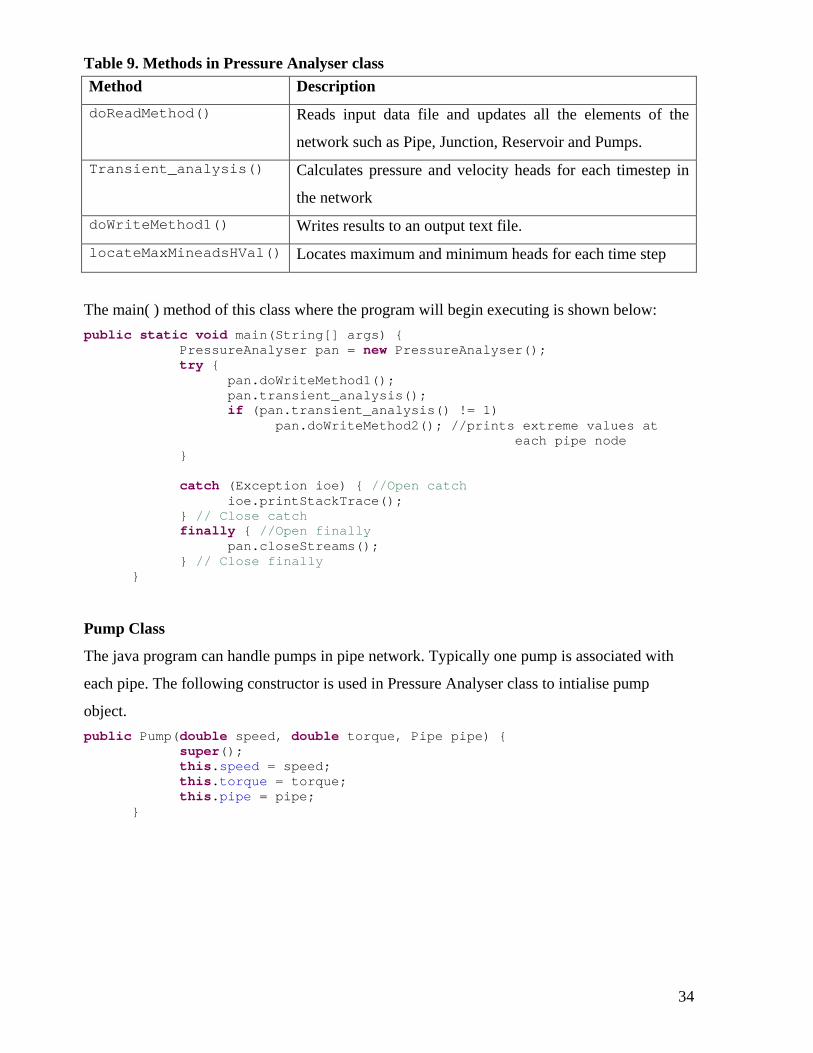
34
Table 9. Methods in Pressure Analyser class Method Description doReadMethod() Reads input data file and updates all the elements of the
network such as Pipe, Junction, Reservoir and Pumps. Transient_analysis() Calculates pressure and velocity heads for each timestep in
the network doWriteMethod1() Writes results to an output text file. locateMaxMineadsHVal() Locates maximum and minimum heads for each time step
The main( ) method of this class where the program will begin executing is shown below: public static void main(String[] args) { PressureAnalyser pan = new PressureAnalyser(); try { pan.doWriteMethod1(); pan.transient_analysis(); if (pan.transient_analysis() != 1)
pan.doWriteMethod2(); //prints extreme values at each pipe node
} catch (Exception ioe) { //Open catch ioe.printStackTrace(); } // Close catch finally { //Open finally pan.closeStreams(); } // Close finally }
Pump Class
The java program can handle pumps in pipe network. Typically one pump is associated with
each pipe. The following constructor is used in Pressure Analyser class to intialise pump
object. public Pump(double speed, double torque, Pipe pipe) { super(); this.speed = speed; this.torque = torque; this.pipe = pipe; }
35
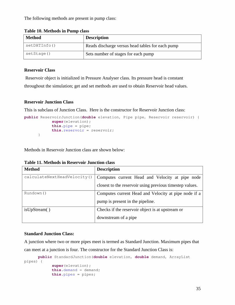
The following methods are present in pump class:
Table 10. Methods in Pump class Method Description setDHTInfo() Reads discharge versus head tables for each pump setStage() Sets number of stages for each pump
Reservoir Class
Reservoir object is initialized in Pressure Analyser class. Its pressure head is constant
throughout the simulation; get and set methods are used to obtain Reservoir head values.
Reservoir Junction Class
This is subclass of Junction Class. Here is the constructor for Reservoir Junction class: public ReservoirJunction(double elevation, Pipe pipe, Reservoir reservoir) { super(elevation); this.pipe = pipe; this.reservoir = reservoir; }
Methods in Reservoir Junction class are shown below:
Table 11. Methods in Reservoir Junction class Method Description calculateNextHeadVelocity() Computes current Head and Velocity at pipe node
closest to the reservoir using previous timestep values. Rundown() Computes current Head and Velocity at pipe node if a
pump is present in the pipeline.
isUpStream( ) Checks if the reservoir object is at upstream or
downstream of a pipe
Standard Junction Class:
A junction where two or more pipes meet is termed as Standard Junction. Maximum pipes that
can meet at a junction is four. The constructor for the Standard Junction Class is: public StandardJunction(double elevation, double demand, ArrayList pipes) { super(elevation); this.demand = demand; this.pipes = pipes;
36
}
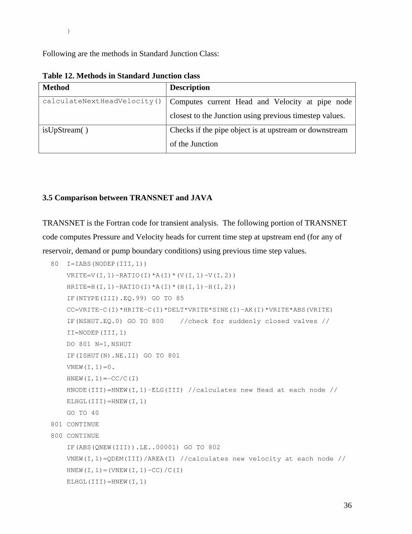
Following are the methods in Standard Junction Class:
Table 12. Methods in Standard Junction class Method Description calculateNextHeadVelocity() Computes current Head and Velocity at pipe node
closest to the Junction using previous timestep values.
isUpStream( ) Checks if the pipe object is at upstream or downstream
of the Junction
3.5 Comparison between TRANSNET and JAVA
TRANSNET is the Fortran code for transient analysis. The following portion of TRANSNET
code computes Pressure and Velocity heads for current time step at upstream end (for any of
reservoir, demand or pump boundary conditions) using previous time step values. 80 I=IABS(NODEP(III,1))
VRITE=V(I,1)-RATIO(I)*A(I)*(V(I,1)-V(I,2))
HRITE=H(I,1)-RATIO(I)*A(I)*(H(I,1)-H(I,2))
IF(NTYPE(III).EQ.99) GO TO 85
CC=VRITE-C(I)*HRITE-C(I)*DELT*VRITE*SINE(I)-AK(I)*VRITE*ABS(VRITE)
IF(NSHUT.EQ.0) GO TO 800 //check for suddenly closed valves //
II=NODEP(III,1)
DO 801 N=1,NSHUT
IF(ISHUT(N).NE.II) GO TO 801
VNEW(I,1)=0.
HNEW(I,1)=-CC/C(I)
HNODE(III)=HNEW(I,1)-ELG(III) //calculates new Head at each node //
ELHGL(III)=HNEW(I,1)
GO TO 40
801 CONTINUE
800 CONTINUE
IF(ABS(QNEW(III)).LE..00001) GO TO 802
VNEW(I,1)=QDEM(III)/AREA(I) //calculates new velocity at each node //
HNEW(I,1)=(VNEW(I,1)-CC)/C(I)
ELHGL(III)=HNEW(I,1)
37
GO TO 40
802 HNEW(I,1)=ELHGL(III)
VNEW(I,1)=CC+C(I)*HNEW(I,1)
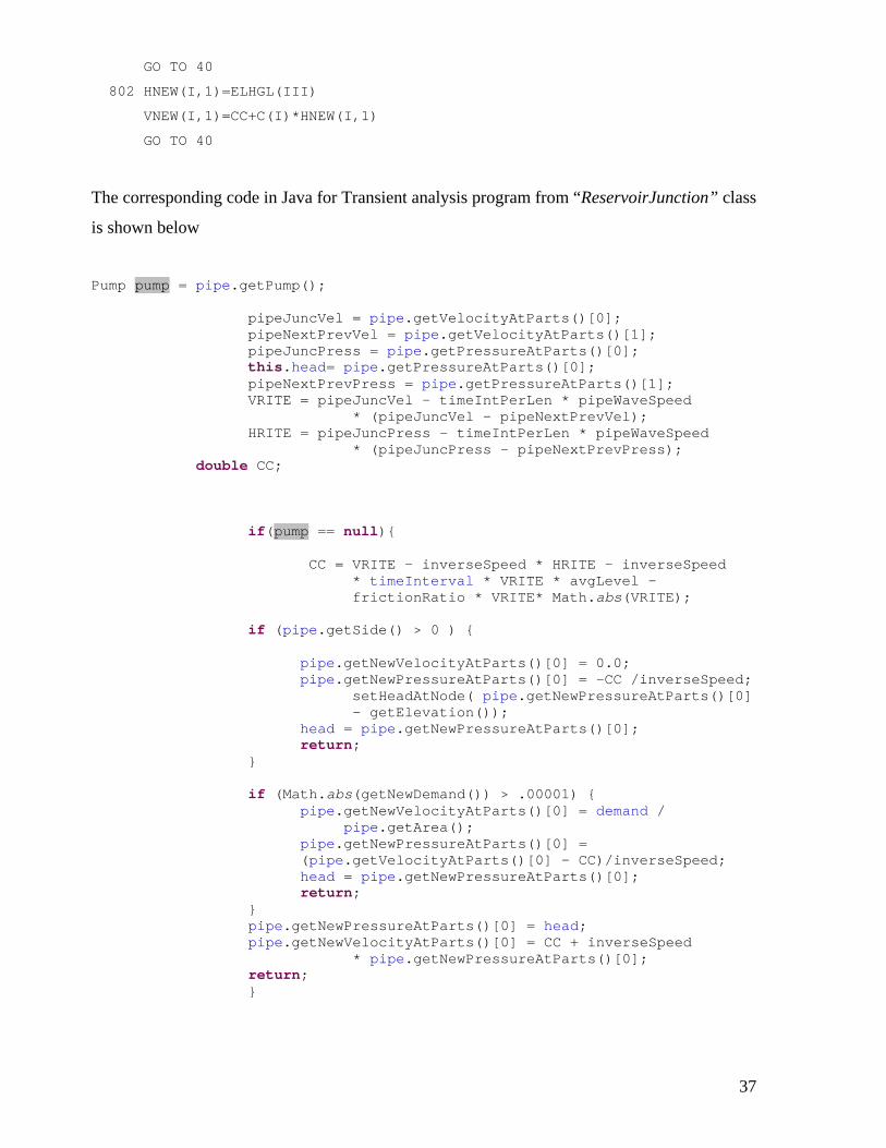
GO TO 40
The corresponding code in Java for Transient analysis program from “ReservoirJunction” class
is shown below
Pump pump = pipe.getPump(); pipeJuncVel = pipe.getVelocityAtParts()[0]; pipeNextPrevVel = pipe.getVelocityAtParts()[1]; pipeJuncPress = pipe.getPressureAtParts()[0]; this.head= pipe.getPressureAtParts()[0]; pipeNextPrevPress = pipe.getPressureAtParts()[1]; VRITE = pipeJuncVel - timeIntPerLen * pipeWaveSpeed * (pipeJuncVel - pipeNextPrevVel); HRITE = pipeJuncPress - timeIntPerLen * pipeWaveSpeed * (pipeJuncPress - pipeNextPrevPress); double CC; if(pump == null){ CC = VRITE - inverseSpeed * HRITE - inverseSpeed
* timeInterval * VRITE * avgLevel - frictionRatio * VRITE* Math.abs(VRITE);
if (pipe.getSide() > 0 ) { pipe.getNewVelocityAtParts()[0] = 0.0; pipe.getNewPressureAtParts()[0] = -CC /inverseSpeed;
setHeadAtNode( pipe.getNewPressureAtParts()[0] - getElevation());
head = pipe.getNewPressureAtParts()[0]; return; } if (Math.abs(getNewDemand()) > .00001) { pipe.getNewVelocityAtParts()[0] = demand / pipe.getArea(); pipe.getNewPressureAtParts()[0] = (pipe.getVelocityAtParts()[0] - CC)/inverseSpeed; head = pipe.getNewPressureAtParts()[0]; return; } pipe.getNewPressureAtParts()[0] = head; pipe.getNewVelocityAtParts()[0] = CC + inverseSpeed * pipe.getNewPressureAtParts()[0]; return; }
38
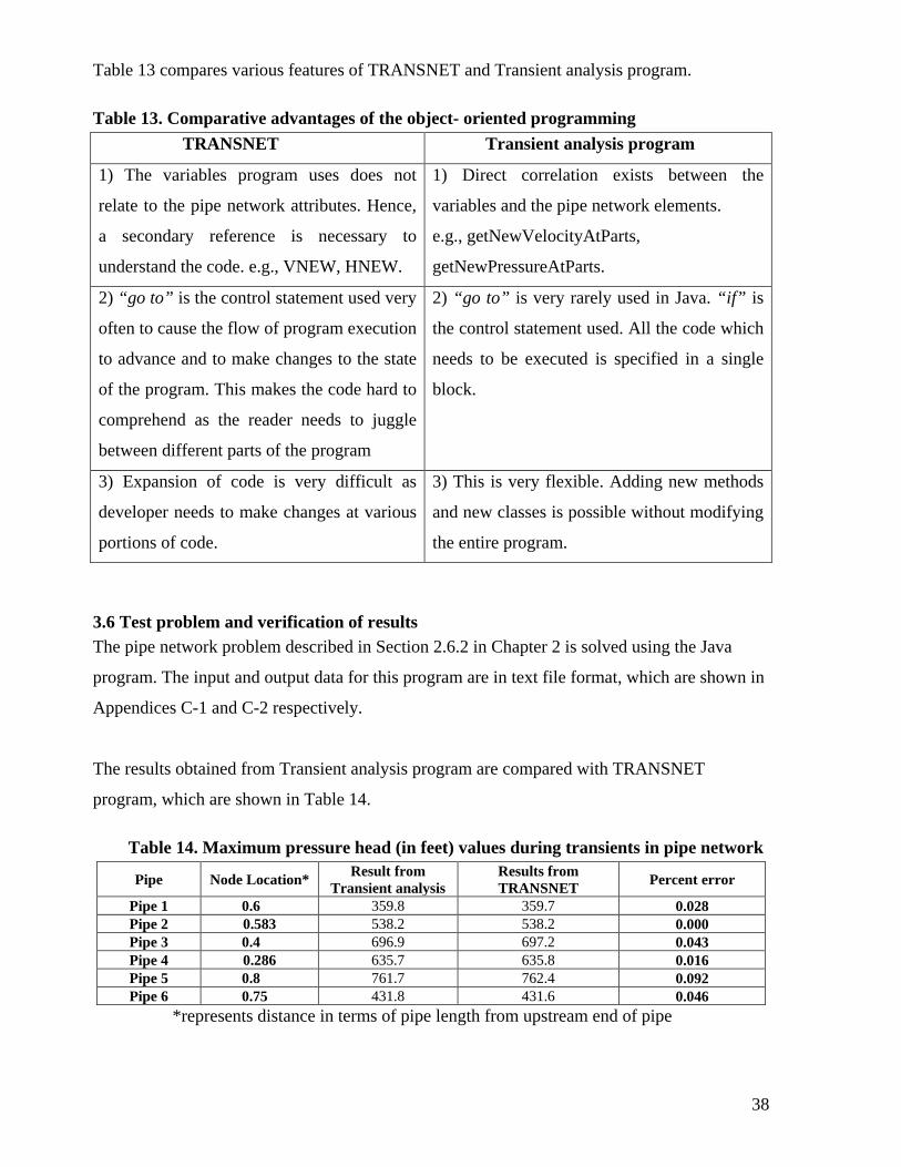
Table 13 compares various features of TRANSNET and Transient analysis program.
Table 13. Comparative advantages of the object- oriented programming TRANSNET Transient analysis program
1) The variables program uses does not
relate to the pipe network attributes. Hence,
a secondary reference is necessary to
understand the code. e.g., VNEW, HNEW.
1) Direct correlation exists between the
variables and the pipe network elements.
e.g., getNewVelocityAtParts,
getNewPressureAtParts.
2) “go to” is the control statement used very
often to cause the flow of program execution
to advance and to make changes to the state
of the program. This makes the code hard to
comprehend as the reader needs to juggle
between different parts of the program
2) “go to” is very rarely used in Java. “if” is
the control statement used. All the code which
needs to be executed is specified in a single
block.
3) Expansion of code is very difficult as
developer needs to make changes at various
portions of code.
3) This is very flexible. Adding new methods
and new classes is possible without modifying
the entire program.
3.6 Test problem and verification of results The pipe network problem described in Section 2.6.2 in Chapter 2 is solved using the Java
program. The input and output data for this program are in text file format, which are shown in
Appendices C-1 and C-2 respectively.
The results obtained from Transient analysis program are compared with TRANSNET
program, which are shown in Table 14.
Table 14. Maximum pressure head (in feet) values during transients in pipe network
Pipe Node Location* Result from Transient analysis
Results from TRANSNET Percent error
Pipe 1 0.6 359.8 359.7 0.028 Pipe 2 0.583 538.2 538.2 0.000 Pipe 3 0.4 696.9 697.2 0.043 Pipe 4 0.286 635.7 635.8 0.016 Pipe 5 0.8 761.7 762.4 0.092 Pipe 6 0.75 431.8 431.6 0.046
*represents distance in terms of pipe length from upstream end of pipe

39
The results from Transient analysis program and TRANSNET program are quite comparable.
However, the slight difference in values between these two programs is due to the rounding
error. All the values calculated in Java are third decimal accurate where as in TRANSNET
computations are done until first decimal only.
40
Chapter 4: Modeling Transient Gaseous Cavitation in Pipes
4.1 Introduction During transient flow of liquid in pipelines, pressures sufficiently less than the saturation
pressure of dissolved gas can be reached. As a result, gas bubbles are formed due to diffusion
of cavitation nuclei. In this process of gas release, free gas volume increases. Consequently, the
mixture celerity is reduced due to added compressibility of the gas, which in turn may give rise
to significant pressure wave dispersion.
The decision to account for gas release (Wiggert and Sundquist, 1979) during a pressure
transient in a pipe depends upon the system dimensions, type of fluid mixture being
transported, extent of saturation of the gas, and low pressure residence times. In long pipelines
where big elevation difference exists at different sections of pipe, transient pressures below gas
saturation pressure is possible. Also, in highly soluble solutions such as water and carbon
dioxide or hydraulic oil and air, significant gas release can take place and should be considered
to correctly simulate the transient. Examples of gaseous cavitation are found in large-scale
cooling water units, aviation fuel lines, and hydraulic control systems.
In present work, a two dimensional (2D) numerical model is developed to analyze gaseous
cavitation in a single pipe system. The model is based on mathematical formulations proposed
by Cannizzaro and Pezzinga (2005) and Pezzinga (2003). The model considers energy
dissipation due to both thermic exhange between gas bubbles and surrounding liquid and
during the process of gas release where as Cannizzaro and Pezzinga (2005) and Pezzinga
(2003) present separate models for thermic exchange and gas release.
The model considers liquid flow with a small amount of free gas. Gas release expression is
derived from Henry’s law. The energy expression in complete form is from Anderson (1995)
and Saurel and Le Metayer (2001). The thermic exchange is expressed from Newton’s law of
cooling (Ewing, 1980). These are the basic equations model uses which undergo several
transformations. Finally, four constitutive equations – rate of mass increase of free gas, the
mixture continuity equation, mixture energy equation, and the mixture momentum – yield a set
41
of differential equations that are solved by the MacCormack (1969) explicit finite-difference
method.
Later, an example is presented to demonstrate this model to analyse transients for the closure
of a downstream valve in a pipe containing an air-water mixture with reservoir upstream.
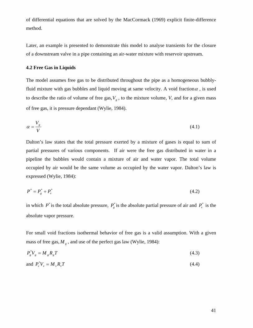
4.2 Free Gas in Liquids The model assumes free gas to be distributed throughout the pipe as a homogeneous bubbly-
fluid mixture with gas bubbles and liquid moving at same velocity. A void fractionα , is used
to describe the ratio of volume of free gas, gV , to the mixture volume, V, and for a given mass
of free gas, it is pressure dependant (Wylie, 1984).
VVg=α (4.1)
Dalton’s law states that the total pressure exerted by a mixture of gases is equal to sum of
partial pressures of various components. If air were the free gas distributed in water in a
pipeline the bubbles would contain a mixture of air and water vapor. The total volume
occupied by air would be the same volume as occupied by the water vapor. Dalton’s law is
expressed (Wylie, 1984):
***
vg PPP += (4.2) in which *P is the total absolute pressure, *
gP is the absolute partial pressure of air and *vP is the
absolute vapor pressure.
For small void fractions isothermal behavior of free gas is a valid assumption. With a given
mass of free gas, gM , and use of the perfect gas law (Wylie, 1984):
TRMVP gggg =* (4.3)
and TRMVP vvvv =* (4.4)
42
In which gV is the gas volume, gR is the gas constant, T is the absolute temperature, vV is the
vapor volume and is equal to the free gas volume, vM is mass of vapor and vR is the vapor gas
constant.
We define mass of free gas per unit volume of the mixture as:
VM
m g= (4.5)
But from above, TRVPM gggg /*= . Therefore, m can be rewritten as:
TVRVP
mg
gg*
= (4.6)
Hence, from above:
*g
gg
PTmR
VV
==α (4.7)
From (4.5) and (4.7)
αρ m
VM
gg
g == (4.8)
4.3 Rate of Gas Release During low pressure periods, gas release takes place and should be considered to correctly
simulate the transient. The present model accommodates for gas release using Henry’s law.
Henry’s law: The amount of gas dissolved in a liquid is proportional to the partial pressure of
gas above the liquid(www).
WH CKP = (4.9)
Where HK is the Henry’s law constant, P is the partial pressure of gas and wC is concentration
of dissolved gas in ./ Lmol
The dimensionless Henry’s law constant, '
HK is defined as
43
w
aH C
CK =' (4.10)
aC is the concentration in gas phase. Using nRTPV = and aCVn= we have
RTPCa = (4.11)
From Eqs. 4.9, 4.10 and 4.11 we have
RTKK H
H =' (4.12)
Mass of dissolved gas in aqueous phase, MVCm lwaq =
MVRTK
PMVKPMVCm l
Hl
Hlwaq '=== (4.13)
The increase in mass of free gas = aqsaq mm −,
][', ppRTKMV
mm sH
laqsaq −=− (4.14)
Where saqm , is the initial mass of free gas present at equilibrium, and sp is the saturation or
equilibrium pressure. Hence, the rate of increase in mass of free gas is given by:
][1'
, ppRTKt
MVt
mmtm
sH
laqsaq −∆
=∆
−=
∂∂ (4.15)
4.4 Energy Equation of gas as function of Temperature and Pressure The energy equation for a gas of unit mass is written as (Anderson, 1995):
dUpdVdq =− (4.16) Where dq is the heat added in Joules, dWpdV = is the work done by the gas in Joules, dU is
the change in internal energy in Joules.
dtdVp
dtdU
dtdq
+= (4.17)
From the definition of enthalpy (Anderson, 1995)
44
pVUh += (4.18)
Where h is the enthalpy per unit mass.
dtdpV
dtdVp
dtdU
dtdh
++= (4.19)
As we are considering unit mass of gas, gV ρ1= where, gρ is the density of gas. Hence, above equation can be written as:
dtdp
dtdVp
dtdU
dtdh
gρ1
++= (4.20)
From (4.17) and (4.20)
dtdp
dtdq
dtdh
gρ1
+= (4.21)
The above is another form of expressing energy equation of a gas. From the definition of specific heat at constant pressure, heat Q added to raise the temperature
of a mass of m from 1T to T is (Saurel and Le Metayer, 2001):
Q )( 1TTmcp −= (4.22) For unit mass: )( 1TTcq p −= (4.23)
dtdTc
dtdq
p= (4.24)
4.4.1 Relation between pc and vc
The energy equation for a reversible process of a closed system, ideal gas is (Anderson, 1995):
pdVdUdq += (4.25) Where q is the heat transfer per unit mass, U is the internal energy per unit mass. Ideal gas equation for unit mass of gas can be written as (Anderson, 1995):
45
RTpV = (4.26) At constant pressure, RdTpdV = (4.27) From above:
RdTdUdq += (4.28)
RdTdU
dTdq
+= (4.29)
Specific heat(www) of a gas is defined as the amount of heat required to change unit mass of
gas by one degree in temperature.
Hence, specific heat of gas at constant volume vc is dTdq when 0=dV . From energy equation
dUdq = (4.30)
vcdTdU
dTdq
== (4.31)
VdppdVpVd +=)( (4.32)
VdppVdpdV −= )( (4.33)
Hence, the above energy equation can be rewritten as:
VdppVddUdq −+= )( (4.34)
VdppVUddq −+= )( (4.35) From the definition of enthalpy, H (Anderson, 1995)
pVUH += (4.36) Therefore at constant pressure, the energy equation is:
dHdq = (4.37) Specific heat of gas at constant pressure pc :
46
pcdTdh
dTdq
== (4.38)
Hence from Eq.s 4.29, 4.31 and 4.38
Rcc vp += (4.39) Let k be the ratio of specific heats,
v
p
cc
k = (4.40)
From Eq.s 4.39 and 4.40
Rk
c p =− )11( (4.41)
Rk
kc p )1( −= (4.42)
4.4.2 Newton’s law of cooling Newton’s Law of Cooling states that the rate of change of temperature of an object is
proportional to the difference between its own temperature and the ambient temperature
(Ewing, 1980).
)( 0TTKdtdT
N −−= (4.43)
Where T is the absolute temperature of the body (gas), 0T is the absolute temperature of the surrounding (liquid), NK is the experimental positive constant (1/sec). Hence, from above:
)( 0TTKcdtdq
Np −−= (4.44)
From Eq. 4.38, dtdTc
dtdh
p= (4.45)
Hence, energy Eq. 4.21 can be written as:
dtdpTTKc
dtdTc
gNpp ρ
1)( 0 +−−= (4.46)
47
Using equation (4.42) in above along with the gas law for gρ , we have
0)()1(0 =−+
−− TTK
dtdp
pT
kk
dtdT
N (4.47)
4.5 One-Dimensional Two-Phase Flow Present model considers the fluid as a homogeneous two-phase air-water mixture. The
properties of the fluid will be average of both components. Following are the assumptions used
in the model:
1) Gas bubbles are distributed throughout the pipe and they are very small compared to
pipe diameter.
2) Difference in pressure due to surface tension across a bubble surface can be neglected;
and
3) Momentum exchange between gas bubbles and surrounding liquid is negligible, so that
gas bubbles and liquid have the same velocity.
4.5.1 Mixture Density The density of a liquid gas mixture, ρ can be expressed as (Wiggert and Sundquist, 1979)
lg ρααρρ )1( −+= (4.48) Where lρ is the liquid density. Using Eq. 4.8, above can be written as:
lm ραρ )1( −+= (4.49)
tttm
t ll
∂∂
−∂−∂
+∂∂
=∂∂ αρ
αρρ )1( (4.50)
Bulk modulus of elasticity of a liquid is given by (Larock, 2000):
llddp
ddpE
ρρνν=−= (4.51)
Also 2/ cE l =ρ (4.52) Hence, we can write:
48
tp
ctp
Etll
∂∂
=∂∂
=∂∂
2
1ρρ (4.53)
Using Eq. 4.53 in Eq. 4.50 we have
tm
tm
pRT
tT
pmR
tp
pmRT
tp
ct l ∂∂
+
∂∂
+∂∂
+∂∂
−−−∂∂
=∂∂
22 )1(1 ραρ (4.54)
−
∂∂
+∂∂
−
+−
∂∂
=∂∂
ρρ
ρρρ
ρρ
αρ
ρρ
lll
pRT
tm
pmR
tT
pmRT
ctp
t1)()1(11
22 (4.55)
For 1<<α and ρρ ≈l we have
−
∂∂
+∂∂
−
+−
∂∂
=∂∂
ρρ
ρρρ
ρρα
ρρ
ρlll
pRT
tm
pmR
tT
pmRT
ctp
t1)()1(11
22 (4.56)
4.5.2 Continuity Equation From one dimensional continuity equation given in Wylie et al.,(1993)
011=
∂∂
++xu
dtdA
Adtdρ
ρ (4.57)
The second term in above equation deals with elasticity of the pipe and its rate of deformation
with pressure. Assuming pipe is rigid dtdA can be scaled to zero. As a consequence, we have
constant area and
xQ
Axu
∂∂
=∂∂ 1 . Where AVQ = (4.58)
Using above expression in continuity equation Eq. 4.57 we have:
011=
∂∂
+
∂∂
+∂∂
xQ
Axu
tρρ
ρ (4.59)
Also neglecting the spatial derivative of density in above continuity equation we have,
49
011=
∂∂
+∂∂
xQ
Atρ
ρ (4.60)
From Eqs. 4.56 and 4.60 continuity equation is finally expressed as:
01222
22
2
=∂∂
+
∂∂
−
−
∂∂
+
+
∂∂
xQ
Ac
pmRc
tT
pRTcc
tm
pmRTc
tp ρρρρ (4.61)
4.6 Conservation form of Mixture Continuity and Energy Equations
Define g
mcpgmRTc
gp
ρρφ
22
+−= (4.62)
tm
gc
tgmc
tT
pgmRc
tm
pgRTc
tp
gmRT
pc
tgp
tp
gt ∂∂
+∂∂
−∂∂
−∂∂
−∂∂
+∂∂
−∂∂
=∂∂
ρρ
ρρ
ρρφ 2
2
222
2
2
2 )(11 (4.63)
Assuming 0≈∂∂
tρ
∂∂
−
−
∂∂
+
+
∂∂
=∂∂
pmR
gc
tT
pRT
gc
gc
tm
pmRT
gc
gtp
t
222
2
21ρρ
φ (4.64)
Using above, mixture continuity equation, Eq. 4.61 is expressed as:
02
=∂∂
+∂∂
xQ
Ac
tg ρφρ (4.65)
Finally, the following conservation form of mixture continuity equation is obtained (Cannizzaro and Pezzinga, 2005):
02
=∂∂
+∂∂
xQ
gAc
tφ (4.66)
Define gas entropy
−
−= pk
kTcs p ln1ln (4.67)
50
∂∂−
−∂∂
=∂∂
tp
pkk
tT
Tc
ts
p111 (4.68)
From energy equation, Eq. 4.47, which is:
0)()1(0 =−+
−− TTK
dtdp
pT
kk
dtdT
N
0)(1)1(10 =−+
−− TTK
dtdp
pkk
dtdT
TT N (4.69)
From Eq.s 4.68 and 4.69 we have
0)(10 =−+
∂∂ TTK
ts
cT N
p
(4.70)
0)1( 0 =−+∂∂
TT
Kcts
Np (4.71)
The conservation form of Energy equation is (Cannizzaro and Pezzinga, 2005):
)1( 0 −=∂∂
TT
Kcts
Np (4.72)
4.7 Mixture Momentum Equation The following momentum equations are written for an elastic pipe with circular cross section,
and assume a 2D flow field with axial symmetry (Pezzinga, 1999).
Along longitudinal direction, x-axis momentum equation:
rr
rxxp
ruv
xuu
tu x
∂∂
−∂∂
−∂∂
−=
∂∂
+∂∂
+∂∂ )(1 τσ
ρ (4.73)
Along radial direction, r-component momentum equation:
rrr
rxrp
rvv
xvu
tv r θσστρ +
∂∂
−∂∂
−∂∂
−=
∂∂
+∂∂
+∂∂ )(1 (4.74)
51
For laminar and turbulent unsteady flows, radial velocity component has values of
order sm /2010 µ− . Hence, in above momentum equations radial velocity v and its derivatives
are neglected. Also, in the momentum equation, in the longitudinal direction the normal stress
is assumed to be equal to the pressure and residual convection term is neglected as usually
done also in 1D models.
The x-axis momentum equation can be rewritten as:
0)(1=
∂∂
+∂∂
+∂∂
rr
rxp
tu τρ (4.75)
Neglecting the stress terms in the radial momentum equation can be written as:
0=∂∂
rp (4.76)
4.7.1 Stress Model Selection of appropriate stress model is important to estimate the initial velocity profile. In the
present gaseous cavitation model for turbulent flow, a two-zone model is considered. In the
viscous sub layer Newton’s law is used and in turbulent zone, Prandtl mixing length hypothesis
(Pezzinga, 1999), namely:
ru
rul
ru
∂∂
∂∂
−∂∂
−= 2ρρντ (4.77)
is used. In above, ν = kinematic viscosity and l = mixing length. For the mixing length the
following expression was adopted (Pezzinga, 1999):
)(
00
0RyeRy
Rl −= κ (4.78)
Where y = distance from wall, 0R = pipe radius; and κ = constant. The following expression
(Pezzinga, 1999) is used to obtainκ .
)100,831ln(0132.0374.0ℜ
++=κ (4.79)
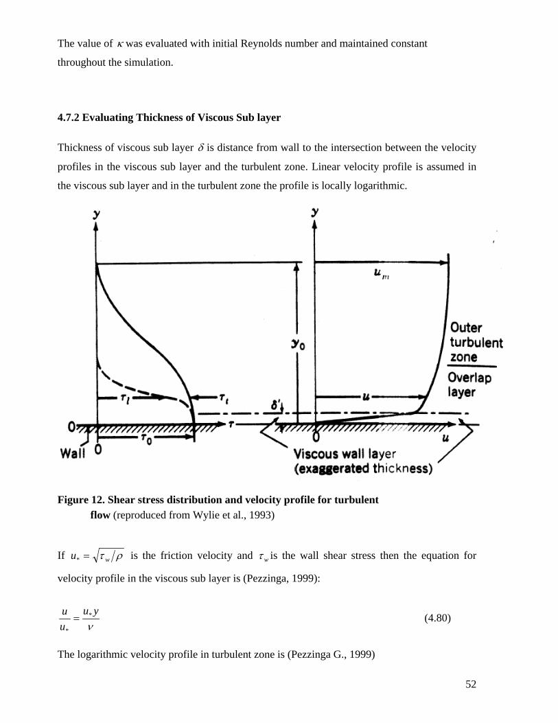
52
The value of κ was evaluated with initial Reynolds number and maintained constant
throughout the simulation.
4.7.2 Evaluating Thickness of Viscous Sub layer Thickness of viscous sub layer δ is distance from wall to the intersection between the velocity
profiles in the viscous sub layer and the turbulent zone. Linear velocity profile is assumed in
the viscous sub layer and in the turbulent zone the profile is locally logarithmic.
Figure 12. Shear stress distribution and velocity profile for turbulent flow (reproduced from Wylie et al., 1993)
If ρτ wu =* is the friction velocity and wτ is the wall shear stress then the equation for
velocity profile in the viscous sub layer is (Pezzinga, 1999):
νyu
uu *
*
= (4.80)
The logarithmic velocity profile in turbulent zone is (Pezzinga G., 1999)
53
0.5ln5.2*
+=εy
uu (4.81)
Viscous sub layer thickness is obtained from the following expression (Streeter and Wylie 1985)
*/63.11 uνδ = (4.82)
4.7.3 Boundary Conditions With regard to the wall condition, if first grid mesh close to the wall is in viscous sub layer
then Eq. 4.80 is used to calculate the wall shear stress wτ otherwise, Eq. 4.81 is used.
On the pipe axis, symmetry condition is adopted. The initial velocity profile was determined by
an iterative procedure, using the unsteady-flow momentum equation and constant discharge.
The initial values of discharge in the pipe and heads at the nodes were obtained from steady-
state conditions.
4.8 Finite Difference Scheme The pipe is divided into cylindrical grid elements of constant length x∆ in longitudinal
direction and constant area A∆ in radial direction. Velocities are defined at center of each
radial mesh, and shear stresses on internal and external sides. Other parameters such as
pressure head H , mass m, Temperature T, φ and s vary along longitudinal direction only and
are defined at each grid point.
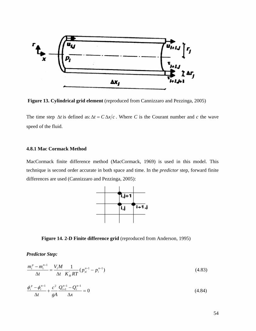
54
Figure 13. Cylindrical grid element (reproduced from Cannizzaro and Pezzinga, 2005)
The time step t∆ is defined as: cxCt ∆=∆ . Where C is the Courant number and c the wave
speed of the fluid.
4.8.1 Mac Cormack Method MacCormack finite difference method (MacCormack, 1969) is used in this model. This
technique is second order accurate in both space and time. In the predictor step, forward finite
differences are used (Cannizzaro and Pezzinga, 2005):
Figure 14. 2-D Finite difference grid (reproduced from Anderson, 1995)
Predictor Step:
)(1 11'
1−−
−
−∆
=∆− n
insi
H
lni
pi pp
RTKtMV
tmm
(4.83)
011
121
=∆−
+∆− −−
+−
xQQ
gAc
t
ni
ni
ni
pi φφ
(4.84)
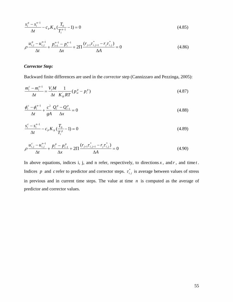
55
0)1( 10
1
=−−∆−
−
−
ni
NP
ni
pi
TT
Kctss
(4.85)
0)(
2*,
*1,1
111
1,, =
∆
−Π+
∆−
+∆
− ++−−
+−
Arr
xpp
tuu jijjij
ni
ni
nji
pji ττ
ρ (4.86)
Corrector Step: Backward finite differences are used in the corrector step (Cannizzaro and Pezzinga, 2005):
)(1'
1pi
psi
H
lni
ci pp
RTKtMV
tmm
−∆
=∆− −
(4.87)
0121
=∆−
+∆− −
−
xQQ
gAc
t
pi
pi
ni
ci φφ
(4.88)
0)1( 01
=−−∆− −
pi
NP
ni
ci
TT
Kctss
(4.89)
0)(
2*,
*1,11
1,, =
∆
−Π+
∆−
+∆
− ++−−
Arr
xpp
tuu jijjij
pi
pi
nji
cji ττ
ρ (4.90)
In above equations, indices i, j, and n refer, respectively, to directions x , and r , and time t .
Indices p and c refer to predictor and corrector steps. *, jiτ is average between values of stress
in previous and in current time steps. The value at time n is computed as the average of
predictor and corrector values.
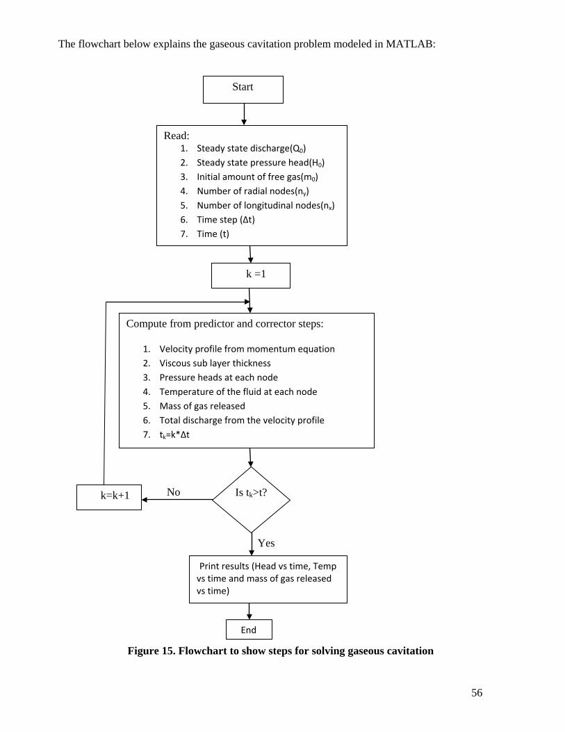
56
The flowchart below explains the gaseous cavitation problem modeled in MATLAB:
Figure 15. Flowchart to show steps for solving gaseous cavitation
Start
Read: 1. Steady state discharge(Q0) 2. Steady state pressure head(H0) 3. Initial amount of free gas(m0) 4. Number of radial nodes(ny) 5. Number of longitudinal nodes(nx) 6. Time step (∆t) 7. Time (t)
Compute from predictor and corrector steps:
1. Velocity profile from momentum equation 2. Viscous sub layer thickness 3. Pressure heads at each node 4. Temperature of the fluid at each node 5. Mass of gas released 6. Total discharge from the velocity profile 7. tk=k*∆t
k =1
Is tk>t?
Yes
Print results (Head vs time, Temp vs time and mass of gas released vs time)
End
No k=k+1
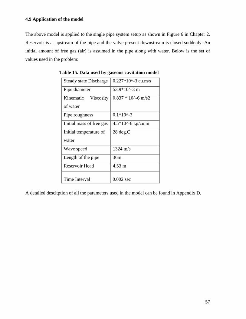
57
4.9 Application of the model
The above model is applied to the single pipe system setup as shown in Figure 6 in Chapter 2.
Reservoir is at upstream of the pipe and the valve present downstream is closed suddenly. An
initial amount of free gas (air) is assumed in the pipe along with water. Below is the set of
values used in the problem:
Table 15. Data used by gaseous cavitation model
A detailed descitption of all the parameters used in the model can be found in Appendix D.
Steady state Discharge 0.227*10^-3 cu.m/s
Pipe diameter 53.9*10^-3 m
Kinematic Viscosity
of water
0.837 * 10^-6 m/s2
Pipe roughness 0.1*10^-3
Initial mass of free gas 4.5*10^-6 kg/cu.m
Initial temperature of
water
28 deg.C
Wave speed 1324 m/s
Length of the pipe 36m
Reservoir Head 4.53 m
Time Interval 0.002 sec
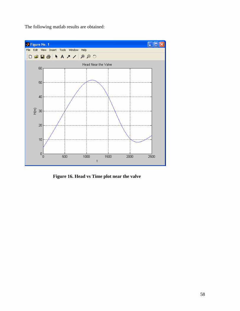
58
The following matlab results are obtained:
Figure 16. Head vs Time plot near the valve
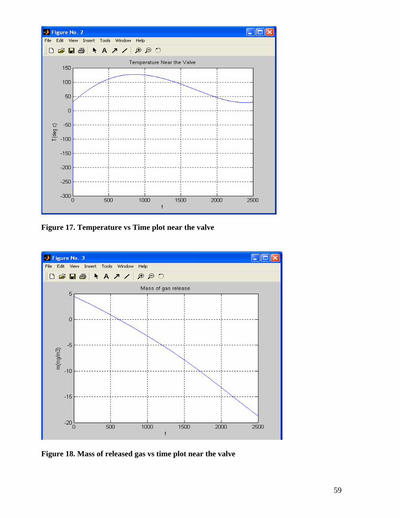
59
Figure 17. Temperature vs Time plot near the valve
Figure 18. Mass of released gas vs time plot near the valve
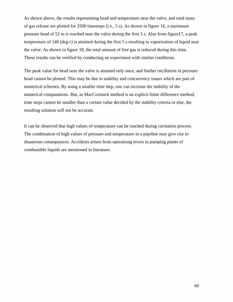
60
As shown above, the results representing head and temperature near the valve, and total mass
of gas release are plotted for 2500 timesteps (i.e., 5 s). As shown in figure 16, a maximum
pressure head of 52 m is reached near the valve during the first 5 s. Also from figure17, a peak
temperature of 140 (deg c) is attained during the first 5 s resulting in vaporization of liquid near
the valve. As shown in figure 18, the total amount of free gas is reduced during this time.
These results can be verified by conducting an experiment with similar conditions.
The peak value for head near the valve is attained only once, and further oscillation in pressure
head cannot be plotted. This may be due to stability and concurrency issues which are part of
numerical schemes. By using a smaller time step, one can increase the stability of the
numerical computations. But, as MacCormack method is an explicit finite difference method,
time steps cannot be smaller than a certain value decided by the stability criteria or else, the
resulting solution will not be accurate.
It can be observed that high values of temperature can be reached during cavitation process.
The combination of high values of pressure and temperature in a pipeline may give rise to
disastrous consequences. Accidents arisen from operationg errors in pumping plants of
combustible liquids are mentioned in literature.
61
Chapter 5: Summary and Conclusions
5.1 Summary
In this thesis, first one dimensional flow in closed conduits was considered to analyse the
changes in pressure and velocity in water distribution system during transient conditions.
Equations related to method of characteristics and finite difference approximations are
discussed. Various boundary conditions such as reservoir, valve, pumps/turbines, and junctions
are considered in the pipe system.
In order to demonstrate the use of method of characterisitics for transient analysis two
problems are solved.
1) A single pipe with reservoir upstream and open valve downstream is considered. In order to
simulate transients, the valve is closed suddenly. An excel spreadsheet is developed to
calculate pressure and velocity heads at each time step. The maximum pressure heads are then
compared with Joukowski’s equation and the results were found comparable. The excel
spreadsheet can be used by any researcher to estimate the critical pressures reached when a
valve is closed suddenly and to measure the total time it takes for pressure waves to die down
and for water to become steady.
2) In order to perform transient analysis in pipe network, a distribution system with six pipes,
three reservoirs, a pump located upstream of one of the reservoirs and a valve at downstream of
one of the pipes is considered. In this network there is a constant demand at three junctions.
Valve is closed suddenly to simulate transient analysis and variations in pressure and velocity
heads are studied in each of the connecting pipes. TRANSNET program is used for transient
analysis and results are compared with WHAMO which gave comparable results for pressure
and velocity head values in pipes.
In Chapter 3, a transient analysis program is developed in Java. This program can analyze
transients caused by suddenly-closing valves, gradually-closing valves, pump power failures
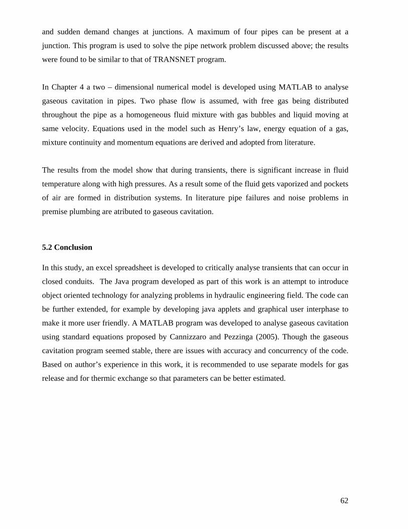
62
and sudden demand changes at junctions. A maximum of four pipes can be present at a
junction. This program is used to solve the pipe network problem discussed above; the results
were found to be similar to that of TRANSNET program.
In Chapter 4 a two – dimensional numerical model is developed using MATLAB to analyse
gaseous cavitation in pipes. Two phase flow is assumed, with free gas being distributed
throughout the pipe as a homogeneous fluid mixture with gas bubbles and liquid moving at
same velocity. Equations used in the model such as Henry’s law, energy equation of a gas,
mixture continuity and momentum equations are derived and adopted from literature.
The results from the model show that during transients, there is significant increase in fluid
temperature along with high pressures. As a result some of the fluid gets vaporized and pockets
of air are formed in distribution systems. In literature pipe failures and noise problems in
premise plumbing are atributed to gaseous cavitation.
5.2 Conclusion In this study, an excel spreadsheet is developed to critically analyse transients that can occur in
closed conduits. The Java program developed as part of this work is an attempt to introduce
object oriented technology for analyzing problems in hydraulic engineering field. The code can
be further extended, for example by developing java applets and graphical user interphase to
make it more user friendly. A MATLAB program was developed to analyse gaseous cavitation
using standard equations proposed by Cannizzaro and Pezzinga (2005). Though the gaseous
cavitation program seemed stable, there are issues with accuracy and concurrency of the code.
Based on author’s experience in this work, it is recommended to use separate models for gas
release and for thermic exchange so that parameters can be better estimated.
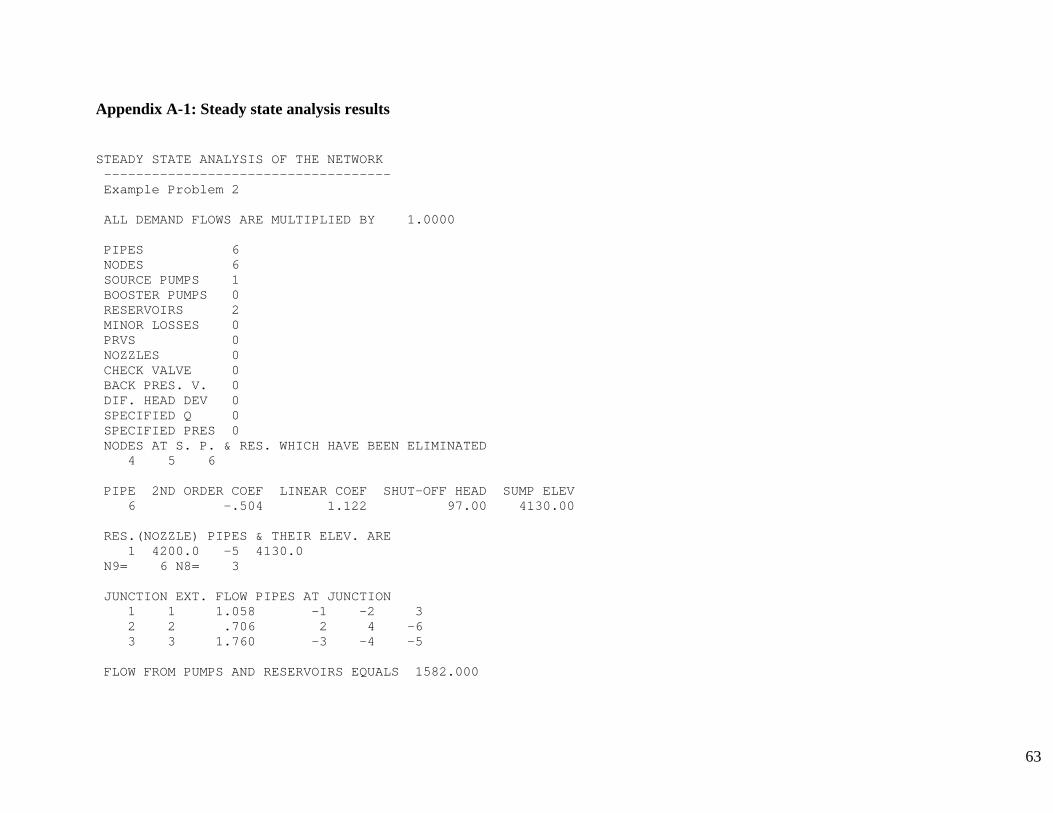
63
Appendix A-1: Steady state analysis results STEADY STATE ANALYSIS OF THE NETWORK ------------------------------------ Example Problem 2 ALL DEMAND FLOWS ARE MULTIPLIED BY 1.0000 PIPES 6 NODES 6 SOURCE PUMPS 1 BOOSTER PUMPS 0 RESERVOIRS 2 MINOR LOSSES 0 PRVS 0 NOZZLES 0 CHECK VALVE 0 BACK PRES. V. 0 DIF. HEAD DEV 0 SPECIFIED Q 0 SPECIFIED PRES 0 NODES AT S. P. & RES. WHICH HAVE BEEN ELIMINATED 4 5 6 PIPE 2ND ORDER COEF LINEAR COEF SHUT-OFF HEAD SUMP ELEV 6 -.504 1.122 97.00 4130.00 RES.(NOZZLE) PIPES & THEIR ELEV. ARE 1 4200.0 -5 4130.0 N9= 6 N8= 3 JUNCTION EXT. FLOW PIPES AT JUNCTION 1 1 1.058 -1 -2 3 2 2 .706 2 4 -6 3 3 1.760 -3 -4 -5 FLOW FROM PUMPS AND RESERVOIRS EQUALS 1582.000
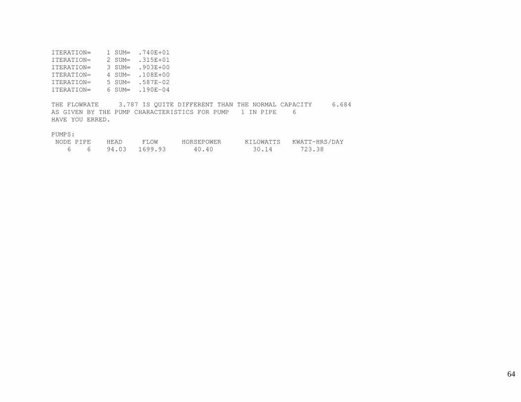
64
ITERATION= 1 SUM= .740E+01 ITERATION= 2 SUM= .315E+01 ITERATION= 3 SUM= .903E+00 ITERATION= 4 SUM= .108E+00 ITERATION= 5 SUM= .587E-02 ITERATION= 6 SUM= .190E-04 THE FLOWRATE 3.787 IS QUITE DIFFERENT THAN THE NORMAL CAPACITY 6.684 AS GIVEN BY THE PUMP CHARACTERISTICS FOR PUMP 1 IN PIPE 6 HAVE YOU ERRED. PUMPS: NODE PIPE HEAD FLOW HORSEPOWER KILOWATTS KWATT-HRS/DAY 6 6 94.03 1699.93 40.40 30.14 723.38
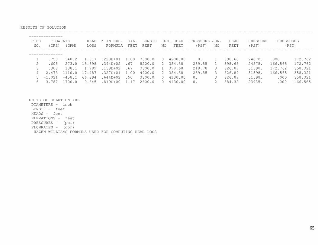
65
RESULTS OF SOLUTION ----------------------------------------------------------------------------------------------------------------------------------- PIPE FLOWRATE HEAD K IN EXP. DIA. LENGTH JUN. HEAD PRESSURE JUN. HEAD PRESSURE PRESSURES NO. (CFS) (GPM) LOSS FORMULA FEET FEET NO FEET (PSF) NO FEET (PSF) (PSI) ----------------------------------------------------------------------------------------------------------------------------------- 1 .758 340.2 1.317 .220E+01 1.00 3300.0 0 4200.00 0. 1 398.68 24878. .000 172.762 2 .608 273.0 15.698 .394E+02 .67 8200.0 2 384.38 239.85 1 398.68 24878. 166.565 172.762 3 .308 138.1 1.789 .159E+02 .67 3300.0 1 398.68 248.78 3 826.89 51598. 172.762 358.321 4 2.473 1110.0 17.487 .327E+01 1.00 4900.0 2 384.38 239.85 3 826.89 51598. 166.565 358.321 5 -1.021 -458.1 66.894 .644E+02 .50 3300.0 0 4130.00 0. 3 826.89 51598. .000 358.321 6 3.787 1700.0 9.645 .819E+00 1.17 2600.0 0 4130.00 0. 2 384.38 23985. .000 166.565 UNITS OF SOLUTION ARE DIAMETERS - inch LENGTH - feet HEADS - feet ELEVATIONS - feet PRESSURES - (psi) FLOWRATES - (gpm) HAZEN-WILLIAMS FORMULA USED FOR COMPUTING HEAD LOSS
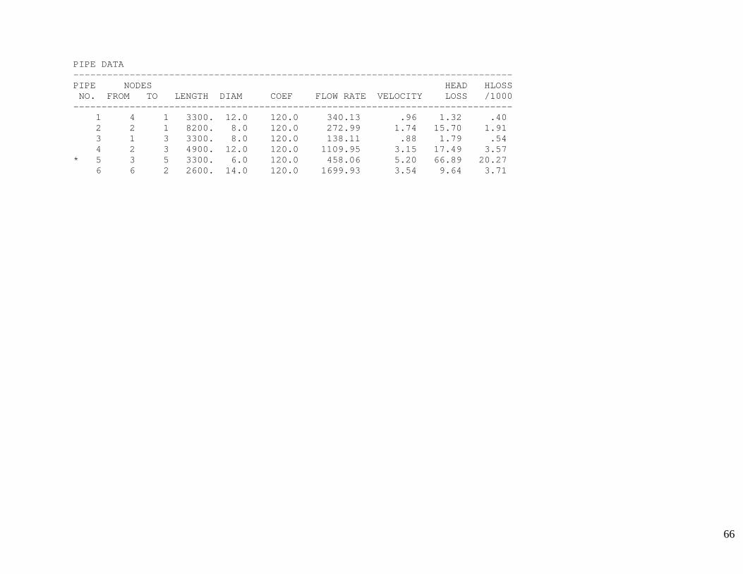
66
PIPE DATA ------------------------------------------------------------------------------ PIPE NODES HEAD HLOSS NO. FROM TO LENGTH DIAM COEF FLOW RATE VELOCITY LOSS /1000 ------------------------------------------------------------------------------ 1 4 1 3300. 12.0 120.0 340.13 .96 1.32 .40 2 2 1 8200. 8.0 120.0 272.99 1.74 15.70 1.91 3 1 3 3300. 8.0 120.0 138.11 .88 1.79 .54 4 2 3 4900. 12.0 120.0 1109.95 3.15 17.49 3.57 * 5 3 5 3300. 6.0 120.0 458.06 5.20 66.89 20.27 6 6 2 2600. 14.0 120.0 1699.93 3.54 9.64 3.71
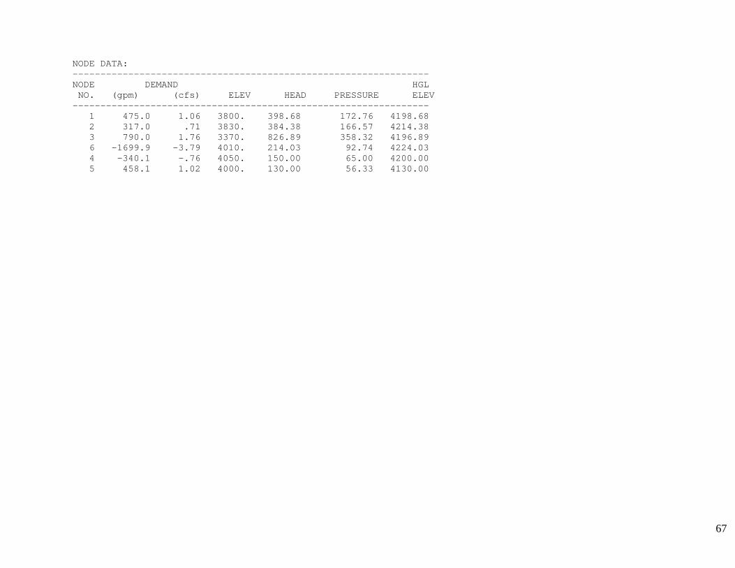
67
NODE DATA: ---------------------------------------------------------------- NODE DEMAND HGL NO. (gpm) (cfs) ELEV HEAD PRESSURE ELEV ---------------------------------------------------------------- 1 475.0 1.06 3800. 398.68 172.76 4198.68 2 317.0 .71 3830. 384.38 166.57 4214.38 3 790.0 1.76 3370. 826.89 358.32 4196.89 6 -1699.9 -3.79 4010. 214.03 92.74 4224.03 4 -340.1 -.76 4050. 150.00 65.00 4200.00 5 458.1 1.02 4000. 130.00 56.33 4130.00
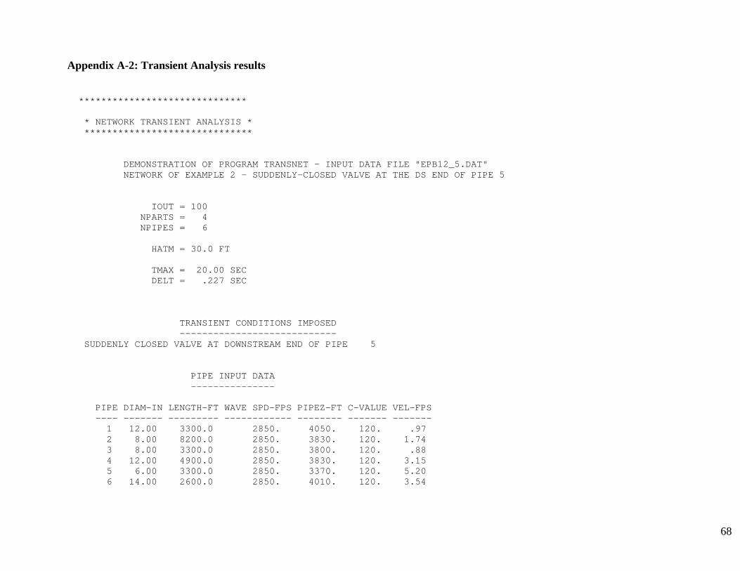
68
Appendix A-2: Transient Analysis results ****************************** * NETWORK TRANSIENT ANALYSIS * ****************************** DEMONSTRATION OF PROGRAM TRANSNET - INPUT DATA FILE "EPB12_5.DAT" NETWORK OF EXAMPLE 2 - SUDDENLY-CLOSED VALVE AT THE DS END OF PIPE 5 IOUT = 100 NPARTS = 4 NPIPES = 6 HATM = 30.0 FT TMAX = 20.00 SEC DELT = .227 SEC TRANSIENT CONDITIONS IMPOSED ---------------------------- SUDDENLY CLOSED VALVE AT DOWNSTREAM END OF PIPE 5 PIPE INPUT DATA --------------- PIPE DIAM-IN LENGTH-FT WAVE SPD-FPS PIPEZ-FT C-VALUE VEL-FPS ---- ------- --------- ------------ -------- ------- ------- 1 12.00 3300.0 2850. 4050. 120. .97 2 8.00 8200.0 2850. 3830. 120. 1.74 3 8.00 3300.0 2850. 3800. 120. .88 4 12.00 4900.0 2850. 3830. 120. 3.15 5 6.00 3300.0 2850. 3370. 120. 5.20 6 14.00 2600.0 2850. 4010. 120. 3.54
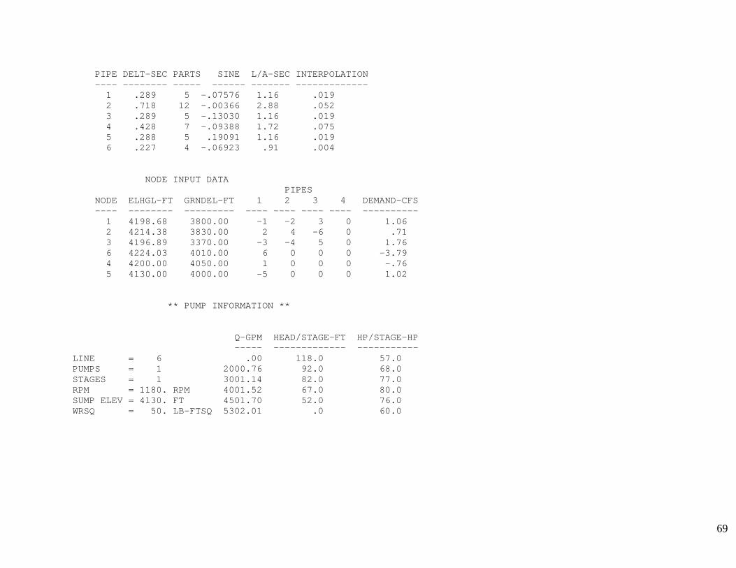
69
PIPE DELT-SEC PARTS SINE L/A-SEC INTERPOLATION ---- -------- ----- ------ ------- ------------- 1 .289 5 -.07576 1.16 .019 2 .718 12 -.00366 2.88 .052 3 .289 5 -.13030 1.16 .019 4 .428 7 -.09388 1.72 .075 5 .288 5 .19091 1.16 .019 6 .227 4 -.06923 .91 .004 NODE INPUT DATA PIPES NODE ELHGL-FT GRNDEL-FT 1 2 3 4 DEMAND-CFS ---- -------- --------- ---- ---- ---- ---- ---------- 1 4198.68 3800.00 -1 -2 3 0 1.06 2 4214.38 3830.00 2 4 -6 0 .71 3 4196.89 3370.00 -3 -4 5 0 1.76 6 4224.03 4010.00 6 0 0 0 -3.79 4 4200.00 4050.00 1 0 0 0 -.76 5 4130.00 4000.00 -5 0 0 0 1.02 ** PUMP INFORMATION ** Q-GPM HEAD/STAGE-FT HP/STAGE-HP ----- ------------- ----------- LINE = 6 .00 118.0 57.0 PUMPS = 1 2000.76 92.0 68.0 STAGES = 1 3001.14 82.0 77.0 RPM = 1180. RPM 4001.52 67.0 80.0 SUMP ELEV = 4130. FT 4501.70 52.0 76.0 WRSQ = 50. LB-FTSQ 5302.01 .0 60.0
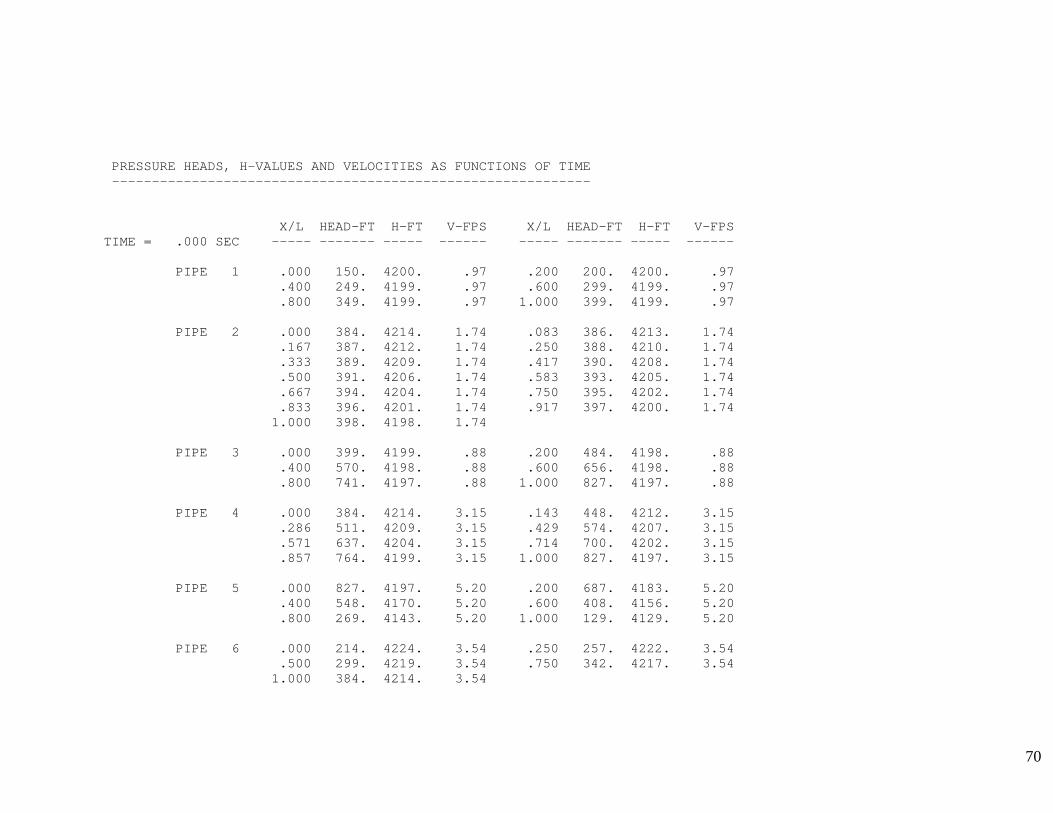
70
PRESSURE HEADS, H-VALUES AND VELOCITIES AS FUNCTIONS OF TIME ------------------------------------------------------------ X/L HEAD-FT H-FT V-FPS X/L HEAD-FT H-FT V-FPS TIME = .000 SEC ----- ------- ----- ------ ----- ------- ----- ------ PIPE 1 .000 150. 4200. .97 .200 200. 4200. .97 .400 249. 4199. .97 .600 299. 4199. .97 .800 349. 4199. .97 1.000 399. 4199. .97 PIPE 2 .000 384. 4214. 1.74 .083 386. 4213. 1.74 .167 387. 4212. 1.74 .250 388. 4210. 1.74 .333 389. 4209. 1.74 .417 390. 4208. 1.74 .500 391. 4206. 1.74 .583 393. 4205. 1.74 .667 394. 4204. 1.74 .750 395. 4202. 1.74 .833 396. 4201. 1.74 .917 397. 4200. 1.74 1.000 398. 4198. 1.74 PIPE 3 .000 399. 4199. .88 .200 484. 4198. .88 .400 570. 4198. .88 .600 656. 4198. .88 .800 741. 4197. .88 1.000 827. 4197. .88 PIPE 4 .000 384. 4214. 3.15 .143 448. 4212. 3.15 .286 511. 4209. 3.15 .429 574. 4207. 3.15 .571 637. 4204. 3.15 .714 700. 4202. 3.15 .857 764. 4199. 3.15 1.000 827. 4197. 3.15 PIPE 5 .000 827. 4197. 5.20 .200 687. 4183. 5.20 .400 548. 4170. 5.20 .600 408. 4156. 5.20 .800 269. 4143. 5.20 1.000 129. 4129. 5.20 PIPE 6 .000 214. 4224. 3.54 .250 257. 4222. 3.54 .500 299. 4219. 3.54 .750 342. 4217. 3.54 1.000 384. 4214. 3.54
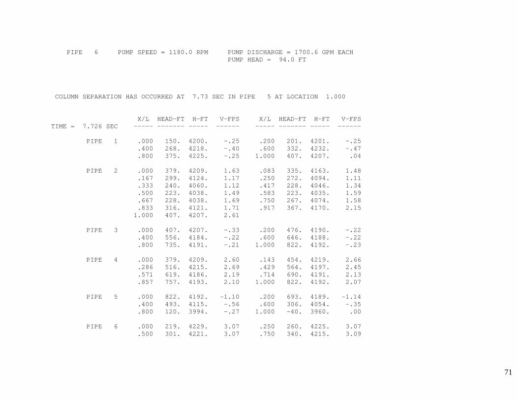
71
PIPE 6 PUMP SPEED = 1180.0 RPM PUMP DISCHARGE = 1700.6 GPM EACH PUMP HEAD = 94.0 FT COLUMN SEPARATION HAS OCCURRED AT 7.73 SEC IN PIPE 5 AT LOCATION 1.000 X/L HEAD-FT H-FT V-FPS X/L HEAD-FT H-FT V-FPS TIME = 7.726 SEC ----- ------- ----- ------ ----- ------- ----- ------ PIPE 1 .000 150. 4200. -.25 .200 201. 4201. -.25 .400 268. 4218. -.40 .600 332. 4232. -.47 .800 375. 4225. -.25 1.000 407. 4207. .04 PIPE 2 .000 379. 4209. 1.63 .083 335. 4163. 1.48 .167 299. 4124. 1.17 .250 272. 4094. 1.11 .333 240. 4060. 1.12 .417 228. 4046. 1.34 .500 223. 4038. 1.49 .583 223. 4035. 1.59 .667 228. 4038. 1.69 .750 267. 4074. 1.58 .833 316. 4121. 1.71 .917 367. 4170. 2.15 1.000 407. 4207. 2.61 PIPE 3 .000 407. 4207. -.33 .200 476. 4190. -.22 .400 556. 4184. -.22 .600 646. 4188. -.22 .800 735. 4191. -.21 1.000 822. 4192. -.23 PIPE 4 .000 379. 4209. 2.60 .143 454. 4219. 2.66 .286 516. 4215. 2.69 .429 564. 4197. 2.45 .571 619. 4186. 2.19 .714 690. 4191. 2.13 .857 757. 4193. 2.10 1.000 822. 4192. 2.07 PIPE 5 .000 822. 4192. -1.10 .200 693. 4189. -1.14 .400 493. 4115. -.56 .600 306. 4054. -.35 .800 120. 3994. -.27 1.000 -40. 3960. .00 PIPE 6 .000 219. 4229. 3.07 .250 260. 4225. 3.07 .500 301. 4221. 3.07 .750 340. 4215. 3.09
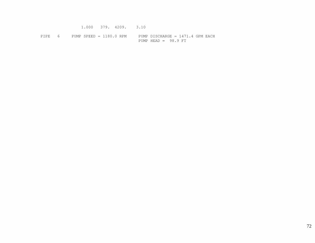
72
1.000 379. 4209. 3.10 PIPE 6 PUMP SPEED = 1180.0 RPM PUMP DISCHARGE = 1471.4 GPM EACH PUMP HEAD = 98.9 FT
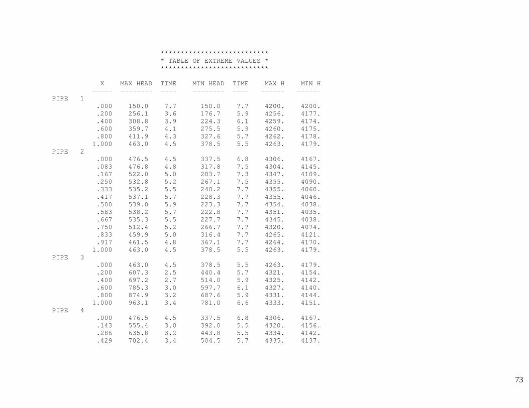
73
*************************** * TABLE OF EXTREME VALUES * *************************** X MAX HEAD TIME MIN HEAD TIME MAX H MIN H ----- -------- ---- -------- ---- ------ ------ PIPE 1 .000 150.0 7.7 150.0 7.7 4200. 4200. .200 256.1 3.6 176.7 5.9 4256. 4177. .400 308.8 3.9 224.3 6.1 4259. 4174. .600 359.7 4.1 275.5 5.9 4260. 4175. .800 411.9 4.3 327.6 5.7 4262. 4178. 1.000 463.0 4.5 378.5 5.5 4263. 4179. PIPE 2 .000 476.5 4.5 337.5 6.8 4306. 4167. .083 476.8 4.8 317.8 7.5 4304. 4145. .167 522.0 5.0 283.7 7.3 4347. 4109. .250 532.8 5.2 267.1 7.5 4355. 4090. .333 535.2 5.5 240.2 7.7 4355. 4060. .417 537.1 5.7 228.3 7.7 4355. 4046. .500 539.0 5.9 223.3 7.7 4354. 4038. .583 538.2 5.7 222.8 7.7 4351. 4035. .667 535.3 5.5 227.7 7.7 4345. 4038. .750 512.4 5.2 266.7 7.7 4320. 4074. .833 459.9 5.0 316.4 7.7 4265. 4121. .917 461.5 4.8 367.1 7.7 4264. 4170. 1.000 463.0 4.5 378.5 5.5 4263. 4179. PIPE 3 .000 463.0 4.5 378.5 5.5 4263. 4179. .200 607.3 2.5 440.4 5.7 4321. 4154. .400 697.2 2.7 514.0 5.9 4325. 4142. .600 785.3 3.0 597.7 6.1 4327. 4140. .800 874.9 3.2 687.6 5.9 4331. 4144. 1.000 963.1 3.4 781.0 6.6 4333. 4151. PIPE 4 .000 476.5 4.5 337.5 6.8 4306. 4167. .143 555.4 3.0 392.0 5.5 4320. 4156. .286 635.8 3.2 443.8 5.5 4334. 4142. .429 702.4 3.4 504.5 5.7 4335. 4137.
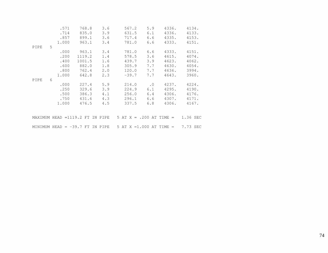
74
.571 768.8 3.6 567.2 5.9 4336. 4134. .714 835.0 3.9 631.5 6.1 4336. 4133. .857 899.1 3.6 717.4 6.6 4335. 4153. 1.000 963.1 3.4 781.0 6.6 4333. 4151. PIPE 5 .000 963.1 3.4 781.0 6.6 4333. 4151. .200 1119.2 1.4 578.5 3.6 4615. 4074. .400 1001.5 1.6 439.7 3.9 4623. 4062. .600 882.0 1.8 305.9 7.7 4630. 4054. .800 762.4 2.0 120.0 7.7 4636. 3994. 1.000 642.8 2.3 -39.7 7.7 4643. 3960. PIPE 6 .000 227.4 5.9 214.0 .0 4237. 4224. .250 329.6 3.9 224.9 6.1 4295. 4190. .500 386.3 4.1 256.0 6.4 4306. 4176. .750 431.6 4.3 296.1 6.6 4307. 4171. 1.000 476.5 4.5 337.5 6.8 4306. 4167. MAXIMUM HEAD =1119.2 FT IN PIPE 5 AT X = .200 AT TIME = 1.36 SEC MINIMUM HEAD = -39.7 FT IN PIPE 5 AT X =1.000 AT TIME = 7.73 SEC
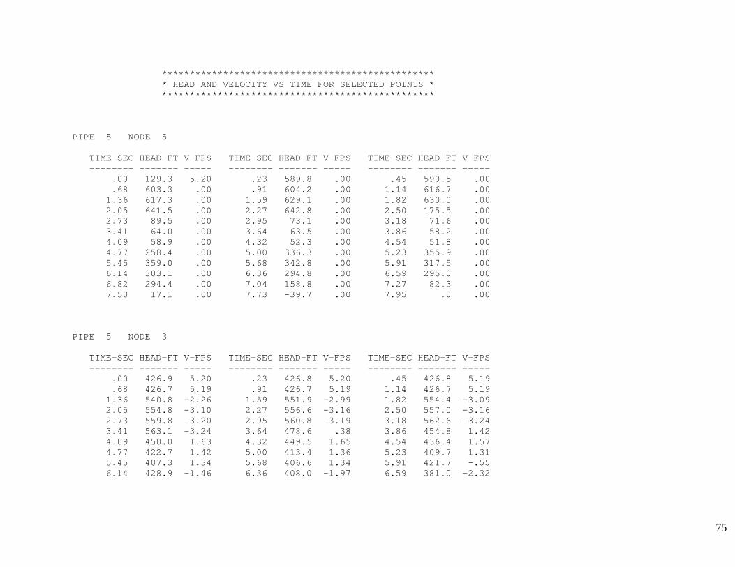
75
************************************************* * HEAD AND VELOCITY VS TIME FOR SELECTED POINTS * ************************************************* PIPE 5 NODE 5 TIME-SEC HEAD-FT V-FPS TIME-SEC HEAD-FT V-FPS TIME-SEC HEAD-FT V-FPS -------- ------- ----- -------- ------- ----- -------- ------- ----- .00 129.3 5.20 .23 589.8 .00 .45 590.5 .00 .68 603.3 .00 .91 604.2 .00 1.14 616.7 .00 1.36 617.3 .00 1.59 629.1 .00 1.82 630.0 .00 2.05 641.5 .00 2.27 642.8 .00 2.50 175.5 .00 2.73 89.5 .00 2.95 73.1 .00 3.18 71.6 .00 3.41 64.0 .00 3.64 63.5 .00 3.86 58.2 .00 4.09 58.9 .00 4.32 52.3 .00 4.54 51.8 .00 4.77 258.4 .00 5.00 336.3 .00 5.23 355.9 .00 5.45 359.0 .00 5.68 342.8 .00 5.91 317.5 .00 6.14 303.1 .00 6.36 294.8 .00 6.59 295.0 .00 6.82 294.4 .00 7.04 158.8 .00 7.27 82.3 .00 7.50 17.1 .00 7.73 -39.7 .00 7.95 .0 .00 PIPE 5 NODE 3 TIME-SEC HEAD-FT V-FPS TIME-SEC HEAD-FT V-FPS TIME-SEC HEAD-FT V-FPS -------- ------- ----- -------- ------- ----- -------- ------- ----- .00 426.9 5.20 .23 426.8 5.20 .45 426.8 5.19 .68 426.7 5.19 .91 426.7 5.19 1.14 426.7 5.19 1.36 540.8 -2.26 1.59 551.9 -2.99 1.82 554.4 -3.09 2.05 554.8 -3.10 2.27 556.6 -3.16 2.50 557.0 -3.16 2.73 559.8 -3.20 2.95 560.8 -3.19 3.18 562.6 -3.24 3.41 563.1 -3.24 3.64 478.6 .38 3.86 454.8 1.42 4.09 450.0 1.63 4.32 449.5 1.65 4.54 436.4 1.57 4.77 422.7 1.42 5.00 413.4 1.36 5.23 409.7 1.31 5.45 407.3 1.34 5.68 406.6 1.34 5.91 421.7 -.55 6.14 428.9 -1.46 6.36 408.0 -1.97 6.59 381.0 -2.32
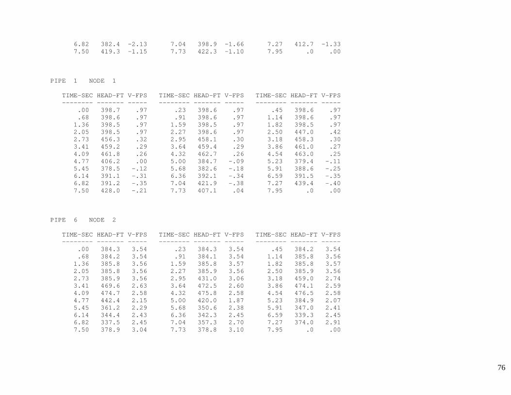
76
6.82 382.4 -2.13 7.04 398.9 -1.66 7.27 412.7 -1.33 7.50 419.3 -1.15 7.73 422.3 -1.10 7.95 .0 .00 PIPE 1 NODE 1 TIME-SEC HEAD-FT V-FPS TIME-SEC HEAD-FT V-FPS TIME-SEC HEAD-FT V-FPS -------- ------- ----- -------- ------- ----- -------- ------- ----- .00 398.7 .97 .23 398.6 .97 .45 398.6 .97 .68 398.6 .97 .91 398.6 .97 1.14 398.6 .97 1.36 398.5 .97 1.59 398.5 .97 1.82 398.5 .97 2.05 398.5 .97 2.27 398.6 .97 2.50 447.0 .42 2.73 456.3 .32 2.95 458.1 .30 3.18 458.3 .30 3.41 459.2 .29 3.64 459.4 .29 3.86 461.0 .27 4.09 461.8 .26 4.32 462.7 .26 4.54 463.0 .25 4.77 406.2 .00 5.00 384.7 -.09 5.23 379.4 -.11 5.45 378.5 -.12 5.68 382.6 -.18 5.91 388.6 -.25 6.14 391.1 -.31 6.36 392.1 -.34 6.59 391.5 -.35 6.82 391.2 -.35 7.04 421.9 -.38 7.27 439.4 -.40 7.50 428.0 -.21 7.73 407.1 .04 7.95 .0 .00 PIPE 6 NODE 2 TIME-SEC HEAD-FT V-FPS TIME-SEC HEAD-FT V-FPS TIME-SEC HEAD-FT V-FPS -------- ------- ----- -------- ------- ----- -------- ------- ----- .00 384.3 3.54 .23 384.3 3.54 .45 384.2 3.54 .68 384.2 3.54 .91 384.1 3.54 1.14 385.8 3.56 1.36 385.8 3.56 1.59 385.8 3.57 1.82 385.8 3.57 2.05 385.8 3.56 2.27 385.9 3.56 2.50 385.9 3.56 2.73 385.9 3.56 2.95 431.0 3.06 3.18 459.0 2.74 3.41 469.6 2.63 3.64 472.5 2.60 3.86 474.1 2.59 4.09 474.7 2.58 4.32 475.8 2.58 4.54 476.5 2.58 4.77 442.4 2.15 5.00 420.0 1.87 5.23 384.9 2.07 5.45 361.2 2.29 5.68 350.6 2.38 5.91 347.0 2.41 6.14 344.4 2.43 6.36 342.3 2.45 6.59 339.3 2.45 6.82 337.5 2.45 7.04 357.3 2.70 7.27 374.0 2.91 7.50 378.9 3.04 7.73 378.8 3.10 7.95 .0 .00
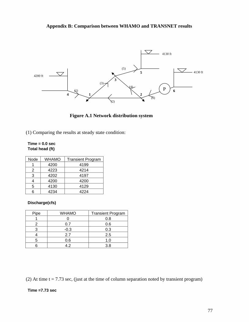
77
Appendix B: Comparison between WHAMO and TRANSNET results
Figure A.1 Network distribution system (1) Comparing the results at steady state condition: Time = 0.0 sec Total head (ft) Node WHAMO Transient Program
1 4200 4199 2 4223 4214 3 4202 4197 4 4200 4200 5 4130 4129 6 4234 4224
Discharge(cfs)
Pipe WHAMO Transient Program 1 0 0.8 2 0.7 0.6 3 -0.3 0.3 4 2.7 2.5 5 0.6 1.0 6 4.2 3.8
(2) At time t = 7.73 sec, (just at the time of column separation noted by transient program) Time =7.73 sec
P
4200 ft
4130 ft
(1)
(2)
(3) (4)
(5)
(6) 1 2
3
4
5
6
4130 ft
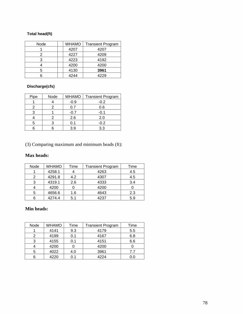
78
Total head(ft)
Node WHAMO Transient Program
1 4207 4207 2 4227 4209 3 4223 4192 4 4200 4200 5 4130 3961 6 4244 4229
Discharge(cfs)
Pipe Node WHAMO Transient Program 1 4 -0.9 -0.2 2 2 0.7 0.6 3 1 -0.7 -0.1 4 2 2.6 2.0 5 3 0.1 -0.2 6 6 3.9 3.3
(3) Comparing maximum and minimum heads (ft): Max heads:
Node WHAMO Time Transient Program Time 1 4258.1 4 4263 4.5 2 4291.8 4.2 4307 4.5 3 4319.1 2.6 4333 3.4 4 4200 0 4200 0 5 4656.6 1.6 4643 2.3 6 4274.4 5.1 4237 5.9
Min heads:
Node WHAMO Time Transient Program Time 1 4141 9.3 4179 5.5 2 4199 0.1 4167 6.8 3 4155 0.1 4151 6.6 4 4200 0 4200 0 5 4022 4.0 3961 7.7 6 4220 0.1 4224 0.0
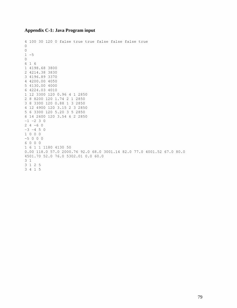
79
Appendix C-1: Java Program input 4 100 30 120 0 false true true false false false true 0 0 1 -5 0 6 1 6 1 4198.68 3800 2 4214.38 3830 3 4196.89 3370 4 4200.00 4050 5 4130.00 4000 6 4224.03 4010 1 12 3300 120 0.96 4 1 2850 2 8 8200 120 1.74 2 1 2850 3 8 3300 120 0.88 1 3 2850 4 12 4900 120 3.15 2 3 2850 5 6 3300 120 5.20 3 5 2850 6 14 2600 120 3.54 6 2 2850 -1 -2 3 0 2 4 -6 0 -3 -4 5 0 1 0 0 0 -5 0 0 0 6 0 0 0 1 6 1 1 1180 4130 50 0.00 118.0 57.0 2000.76 92.0 68.0 3001.14 82.0 77.0 4001.52 67.0 80.0 4501.70 52.0 76.0 5302.01 0.0 60.0 3 1 3 1 2 5 3 4 1 5
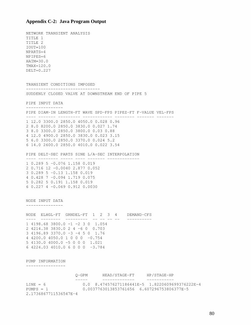
80
Appendix C-2: Java Program Output NETWORK TRANSIENT ANALYSIS TITLE 1 TITLE 2 IOUT=100 NPARTS=4 NPIPES=6 HATM=30.0 TMAX=120.0 DELT=0.227 TRANSIENT CONDITIONS IMPOSED ------------------------------ SUDDENLY CLOSED VALVE AT DOWNSTREAM END OF PIPE 5 PIPE INPUT DATA --------------- PIPE DIAM-IN LENGTH-FT WAVE SPD-FPS PIPEZ-FT F-VALUE VEL-FPS ---- ------- --------- ------------ -------- ------- ------- 1 12.0 3300.0 2850.0 4050.0 0.028 0.96 2 8.0 8200.0 2850.0 3830.0 0.027 1.74 3 8.0 3300.0 2850.0 3800.0 0.03 0.88 4 12.0 4900.0 2850.0 3830.0 0.023 3.15 5 6.0 3300.0 2850.0 3370.0 0.024 5.2 6 14.0 2600.0 2850.0 4010.0 0.022 3.54 PIPE DELT-SEC PARTS SINE L/A-SEC INTERPOLATION ---- -------- ----- ---- ------- ------------- 1 0.289 5 -0.076 1.158 0.019 2 0.716 12 -0.0040 2.877 0.052 3 0.289 5 -0.13 1.158 0.019 4 0.428 7 -0.094 1.719 0.075 5 0.282 5 0.191 1.158 0.019 6 0.227 4 -0.069 0.912 0.0030 NODE INPUT DATA --------------- NODE ELHGL-FT GRNDEL-FT 1 2 3 4 DEMAND-CFS ---- -------- --------- -- -- -- -- ---------- 1 4198.68 3800.0 -1 -2 3 0 1.054 2 4214.38 3830.0 2 4 -6 0 0.703 3 4196.89 3370.0 -3 -4 5 0 1.76 4 4200.0 4050.0 1 0 0 0 -0.754 5 4130.0 4000.0 -5 0 0 0 1.021 6 4224.03 4010.0 6 0 0 0 -3.784 PUMP INFORMATION ---------------- Q-GPM HEAD/STAGE-FT HP/STAGE-HP ----- ------------- ----------- LINE = 6 0.0 8.474576271186441E-5 1.8220609699376222E-4 PUMPS = 1 0.0037763013853761656 6.607296753806377E-5 2.1736867711536547E-4
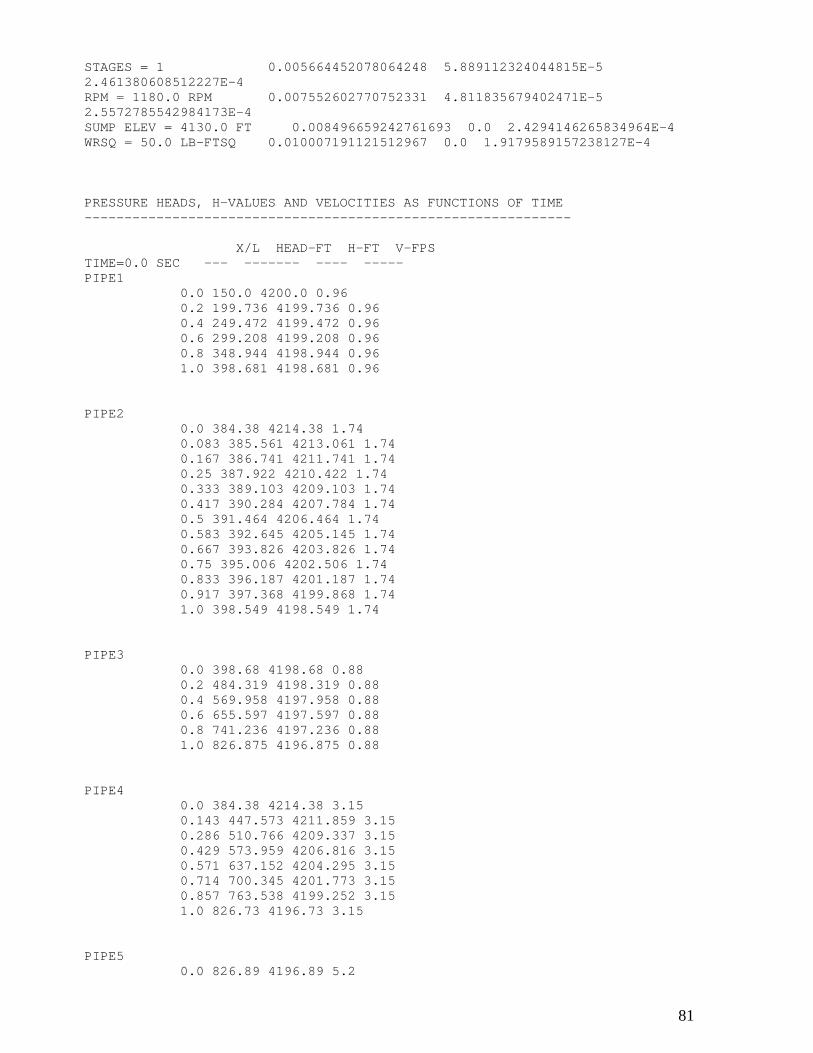
81
STAGES = 1 0.005664452078064248 5.889112324044815E-5 2.461380608512227E-4 RPM = 1180.0 RPM 0.007552602770752331 4.811835679402471E-5 2.5572785542984173E-4 SUMP ELEV = 4130.0 FT 0.008496659242761693 0.0 2.4294146265834964E-4 WRSQ = 50.0 LB-FTSQ 0.010007191121512967 0.0 1.9179589157238127E-4 PRESSURE HEADS, H-VALUES AND VELOCITIES AS FUNCTIONS OF TIME ------------------------------------------------------------- X/L HEAD-FT H-FT V-FPS TIME=0.0 SEC --- ------- ---- ----- PIPE1 0.0 150.0 4200.0 0.96 0.2 199.736 4199.736 0.96 0.4 249.472 4199.472 0.96 0.6 299.208 4199.208 0.96 0.8 348.944 4198.944 0.96 1.0 398.681 4198.681 0.96 PIPE2 0.0 384.38 4214.38 1.74 0.083 385.561 4213.061 1.74 0.167 386.741 4211.741 1.74 0.25 387.922 4210.422 1.74 0.333 389.103 4209.103 1.74 0.417 390.284 4207.784 1.74 0.5 391.464 4206.464 1.74 0.583 392.645 4205.145 1.74 0.667 393.826 4203.826 1.74 0.75 395.006 4202.506 1.74 0.833 396.187 4201.187 1.74 0.917 397.368 4199.868 1.74 1.0 398.549 4198.549 1.74 PIPE3 0.0 398.68 4198.68 0.88 0.2 484.319 4198.319 0.88 0.4 569.958 4197.958 0.88 0.6 655.597 4197.597 0.88 0.8 741.236 4197.236 0.88 1.0 826.875 4196.875 0.88 PIPE4 0.0 384.38 4214.38 3.15 0.143 447.573 4211.859 3.15 0.286 510.766 4209.337 3.15 0.429 573.959 4206.816 3.15 0.571 637.152 4204.295 3.15 0.714 700.345 4201.773 3.15 0.857 763.538 4199.252 3.15 1.0 826.73 4196.73 3.15 PIPE5 0.0 826.89 4196.89 5.2
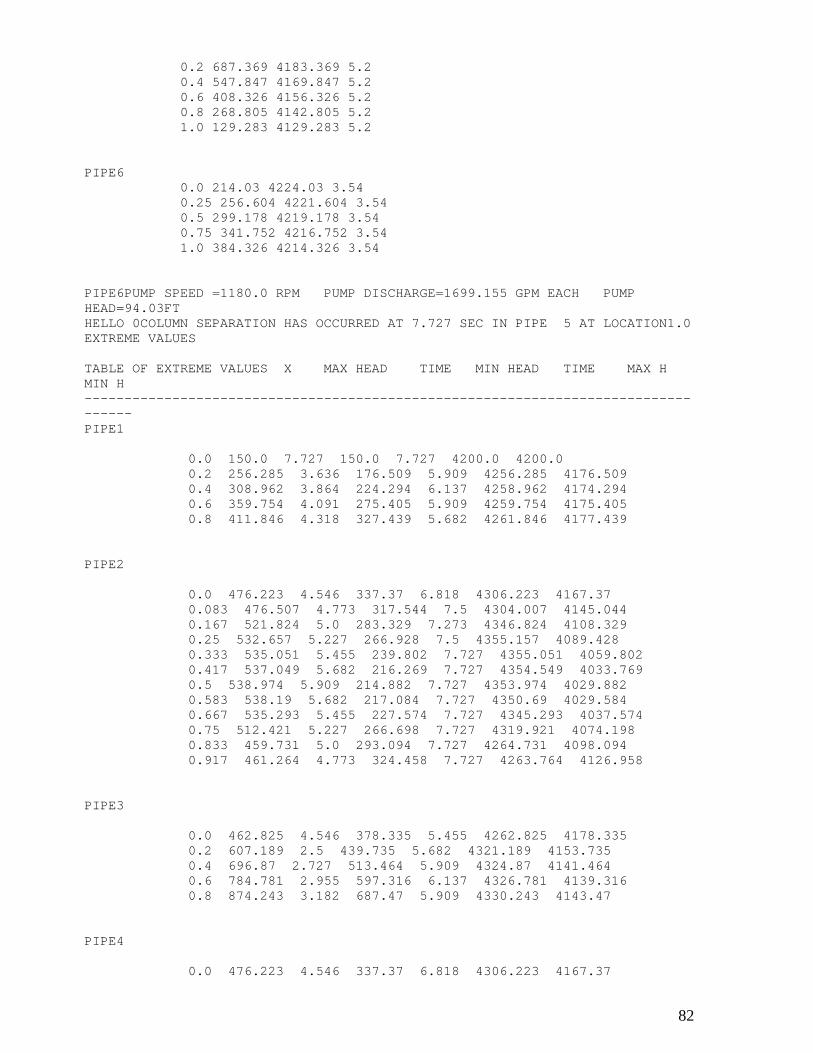
82
0.2 687.369 4183.369 5.2 0.4 547.847 4169.847 5.2 0.6 408.326 4156.326 5.2 0.8 268.805 4142.805 5.2 1.0 129.283 4129.283 5.2 PIPE6 0.0 214.03 4224.03 3.54 0.25 256.604 4221.604 3.54 0.5 299.178 4219.178 3.54 0.75 341.752 4216.752 3.54 1.0 384.326 4214.326 3.54 PIPE6PUMP SPEED =1180.0 RPM PUMP DISCHARGE=1699.155 GPM EACH PUMP HEAD=94.03FT HELLO 0COLUMN SEPARATION HAS OCCURRED AT 7.727 SEC IN PIPE 5 AT LOCATION1.0 EXTREME VALUES TABLE OF EXTREME VALUES X MAX HEAD TIME MIN HEAD TIME MAX H MIN H ---------------------------------------------------------------------------------- PIPE1 0.0 150.0 7.727 150.0 7.727 4200.0 4200.0 0.2 256.285 3.636 176.509 5.909 4256.285 4176.509 0.4 308.962 3.864 224.294 6.137 4258.962 4174.294 0.6 359.754 4.091 275.405 5.909 4259.754 4175.405 0.8 411.846 4.318 327.439 5.682 4261.846 4177.439 PIPE2 0.0 476.223 4.546 337.37 6.818 4306.223 4167.37 0.083 476.507 4.773 317.544 7.5 4304.007 4145.044 0.167 521.824 5.0 283.329 7.273 4346.824 4108.329 0.25 532.657 5.227 266.928 7.5 4355.157 4089.428 0.333 535.051 5.455 239.802 7.727 4355.051 4059.802 0.417 537.049 5.682 216.269 7.727 4354.549 4033.769 0.5 538.974 5.909 214.882 7.727 4353.974 4029.882 0.583 538.19 5.682 217.084 7.727 4350.69 4029.584 0.667 535.293 5.455 227.574 7.727 4345.293 4037.574 0.75 512.421 5.227 266.698 7.727 4319.921 4074.198 0.833 459.731 5.0 293.094 7.727 4264.731 4098.094 0.917 461.264 4.773 324.458 7.727 4263.764 4126.958 PIPE3 0.0 462.825 4.546 378.335 5.455 4262.825 4178.335 0.2 607.189 2.5 439.735 5.682 4321.189 4153.735 0.4 696.87 2.727 513.464 5.909 4324.87 4141.464 0.6 784.781 2.955 597.316 6.137 4326.781 4139.316 0.8 874.243 3.182 687.47 5.909 4330.243 4143.47 PIPE4 0.0 476.223 4.546 337.37 6.818 4306.223 4167.37
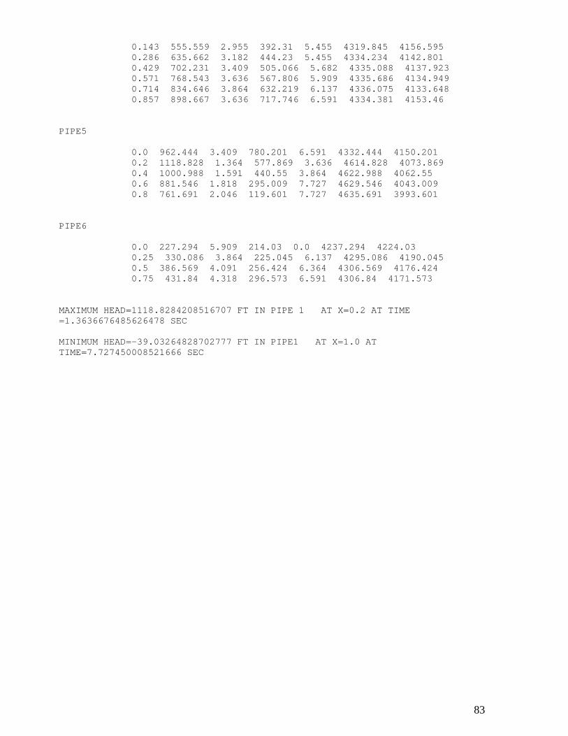
83
0.143 555.559 2.955 392.31 5.455 4319.845 4156.595 0.286 635.662 3.182 444.23 5.455 4334.234 4142.801 0.429 702.231 3.409 505.066 5.682 4335.088 4137.923 0.571 768.543 3.636 567.806 5.909 4335.686 4134.949 0.714 834.646 3.864 632.219 6.137 4336.075 4133.648 0.857 898.667 3.636 717.746 6.591 4334.381 4153.46 PIPE5 0.0 962.444 3.409 780.201 6.591 4332.444 4150.201 0.2 1118.828 1.364 577.869 3.636 4614.828 4073.869 0.4 1000.988 1.591 440.55 3.864 4622.988 4062.55 0.6 881.546 1.818 295.009 7.727 4629.546 4043.009 0.8 761.691 2.046 119.601 7.727 4635.691 3993.601 PIPE6 0.0 227.294 5.909 214.03 0.0 4237.294 4224.03 0.25 330.086 3.864 225.045 6.137 4295.086 4190.045 0.5 386.569 4.091 256.424 6.364 4306.569 4176.424 0.75 431.84 4.318 296.573 6.591 4306.84 4171.573 MAXIMUM HEAD=1118.8284208516707 FT IN PIPE 1 AT X=0.2 AT TIME =1.3636676485626478 SEC MINIMUM HEAD=-39.03264828702777 FT IN PIPE1 AT X=1.0 AT TIME=7.727450008521666 SEC
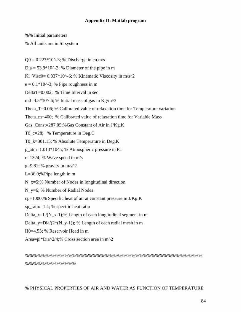
84
Appendix D: Matlab program
%% Initial parameters
% All units are in SI system
Q0 = 0.227*10^-3; % Discharge in cu.m/s
Dia = 53.9*10^-3; % Diameter of the pipe in m
Ki_Visc0= 0.837*10^-6; % Kinematic Viscosity in m/s^2
e = 0.1*10^-3; % Pipe roughness in m
DeltaT=0.002; % Time Interval in sec
m0=4.5*10^-6; % Initial mass of gas in Kg/m^3
Theta_T=0.06; % Calibrated value of relaxation time for Temperature variation
Theta_m=400; % Calibrated value of relaxation time for Variable Mass
Gas_Const=287.05;%Gas Constant of Air in J/Kg.K
T0_c=28; % Temperature in Deg.C
T0_k=301.15; % Absolute Temperature in Deg.K
p_atm=1.013*10^5; % Atmospheric pressure in Pa
c=1324; % Wave speed in m/s
g=9.81; % gravity in m/s^2
L=36.0;%Pipe length in m
N_x=5;% Number of Nodes in longitudinal direction
N_y=6; % Number of Radial Nodes
cp=1000;% Specific heat of air at constant pressure in J/Kg.K
sp_ratio=1.4; % specific heat ratio
Delta_x=L/(N_x-1);% Length of each longitudinal segment in m
Delta_y=Dia/(2*(N_y-1)); % Length of each radial mesh in m
H0=4.53; % Reservoir Head in m
Area=pi*Dia^2/4;% Cross section area in m^2
%%%%%%%%%%%%%%%%%%%%%%%%%%%%%%%%%%%%%%%%%%%%%
%%%%%%%%%%%%%
% PHYSICAL PROPERTIES OF AIR AND WATER AS FUNCTION OF TEMPERATURE
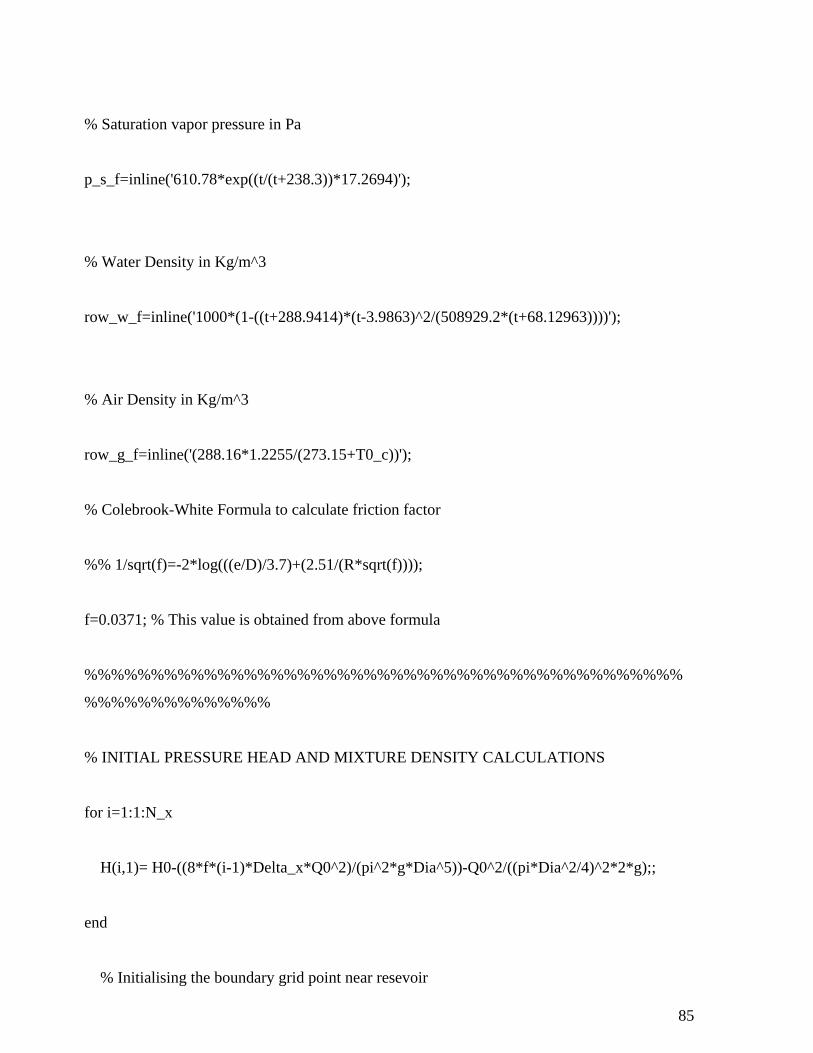
85
% Saturation vapor pressure in Pa
p_s_f=inline('610.78*exp((t/(t+238.3))*17.2694)');
% Water Density in Kg/m^3
row_w_f=inline('1000*(1-((t+288.9414)*(t-3.9863)^2/(508929.2*(t+68.12963))))');
% Air Density in Kg/m^3
row_g_f=inline('(288.16*1.2255/(273.15+T0_c))');
% Colebrook-White Formula to calculate friction factor
%% 1/sqrt(f)=-2*log(((e/D)/3.7)+(2.51/(R*sqrt(f))));
f=0.0371; % This value is obtained from above formula
%%%%%%%%%%%%%%%%%%%%%%%%%%%%%%%%%%%%%%%%%%%%%
%%%%%%%%%%%%%%
% INITIAL PRESSURE HEAD AND MIXTURE DENSITY CALCULATIONS
for i=1:1:N_x
H(i,1)= H0-((8*f*(i-1)*Delta_x*Q0^2)/(pi^2*g*Dia^5))-Q0^2/((pi*Dia^2/4)^2*2*g);;
end
% Initialising the boundary grid point near resevoir
86
p(1,1)=1.418*10^5;
row_w(1,1)=row_w_f(T0_c);
row_g(1,1)=row_g_f(T0_c);
row(1,1)=996.26;
p_s(1,1)=p_s_f(T0_c);
Ki_Visc(1,1)=.837*10^-6;
for i=2:1:N_x-1
row_w(i,1)=row_w_f(T0_c);
row_g(i,1)=row_g_f(T0_c);
p_s(i,1)=p_s_f(T0_c);
m(i,1)=(m0/(N_x-1));
% Solve Quadratic Expression for Absolute Pressure
a=1; b=-(g*H(i,1)*row_w(i,1)+p_atm-p_s(i,1));
c0=g*m(i,1)*Gas_Const*(273.15+T0_c)*H(i,1)*(row_w(i,1)- row_g(i,1));
p(i,1)=(-b+(b^2-4*a*c0)^.5)/(2*a);
% Mixture Density
row(i,1)=(p(i,1)+p_s(i,1)-p_atm)/(H(i,1)*g);
end
%%%%%%%%%%%%%%%%%%%%%%%%%%%%%%%%%%%%%%%%%%%%%
%%%%%%%%%%%%%%
% INITIAL VELOCITY PROFILE CALCULATIONS
87
% Grid points in Radial Direction
for i=1:1:N_y
r_N(i,1)=Dia/2-(Delta_y*(N_y-i));
if i<N_y
r_D(i,1)=r_N(i,1)+Delta_y/2;
else
r_D(i,1)=r_N(i,1);
end
end
% Reynold's Number
R=round((4*Q0)/(pi*Dia*Ki_Visc0));
% Constant K throughout simulation
k=0.374+(.0132*log(1+(83100/R)));
% Delta_A
Delta_A= (1/(N_y-1))*(pi/4)*Dia^2;
for i=2:1:N_x-1
% Friction Velocity
ustar(i,1)=((4*Q0)/(pi*Dia^2))*sqrt(f/8);
% Sublayer thickness
Delta(i,1)=11.63*Ki_Visc0/ustar(i,1);
% Special Parameters
88
Phi(i,1)=(p(i,1)/(row(i,1)*g))-
(c^2*m(i,1)*Gas_Const*(273.15+T0_c)/(g*p(i,1)))+c^2*m(i,1)/(row(i,1)*g);
s(i,1)=cp*(log(273.15+T0_c)-(sp_ratio-1)*log(p(i,1))/sp_ratio);
end
% Validating if a Grid point is in viscous sublayer or in Transient region
% and then obtain the initial velocity profile
for j=N_y:-1:1
u(1,N_y)=0;
end
for i=2:1:N_x-1
for j=N_y:-1:1
if Dia/2-r_D(j,1) <= Delta(i,1)
u(i,j)=ustar(i,1)^2*(Dia/2-r_D(j,1))/Ki_Visc0;
else
u(i,j)=ustar(i,1)*(2.5*log((Dia/2-r_D(j,1))/e)+5.0);
end
l(j,1)=k*(Dia/2-r_N(j,1))*exp(-(Dia/2-r_N(j,1))/(Dia/2));
end
end
t=1;
status=1;
TOL=10^-4;
error=1;
while status<=4
89
for i=2:1:N_x-1
count=0;
flag=0;
Ki_Visc(i,1)=.837*10^-6;
for j=N_y-1:-1:1
if Dia/2-r_N(j,1)<=Delta(i,1)
if j==N_y-1
D(1,i)=(1/DeltaT)+(pi/row(i,t))*(1/Delta_A)*Ki_Visc(i,t)*row_w(i,t)*((r_N(N_y,1)/(r_D(N_y
,1)-r_D(N_y-1,1)))+(r_N(N_y-1,1)/(r_D(N_y-1,1)-r_D(N_y-2-1,1))));
A(1,i)=-pi*r_N(N_y-1,1)*Ki_Visc(i,t)*row_w(i,t)/(row(i,t)*Delta_A*(r_D(N_y-
1,1)-r_D(N_y-2,1)));
C(1,i)=-((-u(i,N_y-1)/DeltaT)+(g*(H(i+1,1)-
H(i,1))/Delta_x)+(pi/row(i,t))*(Ki_Visc(i,t)*row_w(i,t)/Delta_A)*((r_N(N_y,1)*u(i,N_y-
1)/(r_D(N_y,1)-r_D(N_y-1,1)))-(r_N(N_y-1,1)*u(i,N_y-2)/(r_D(N_y-1,1)-r_D(N_y-
2,1)))+(r_N(N_y-1,1)*u(i,N_y-1)/(r_D(N_y-1,1)-r_D(N_y-2,1)))));
flag=flag+1;
else
B(2+count,i)=-
pi*Ki_Visc(i,t)*row_w(i,t)*r_N(j+1,1)/(row(i,t)*Delta_A*(r_D(j+1,1)-r_D(j,1)));
D(2+count,i)=(1/DeltaT)+(pi/row(i,t))*(1/Delta_A)*Ki_Visc(i,t)*row_w(i,t)*((r_N(j+1,1)/(r_
D(j+1,1)-r_D(j,1)))+(r_N(j,1)/(r_D(j,1)-r_D(j-1,1))));
A(2+count,i)=-pi*r_N(j,1)*Ki_Visc(i,t)*row_w(i,t)/(row(i,t)*Delta_A*(r_D(j,1)-
r_D(j-1,1)));
C(2+count,i)=-((-u(i,j)/DeltaT)+(g*(H(i+1,1)-
H(i,1))/Delta_x)+(pi/row(i,t))*(Ki_Visc(i,t)*row_w(i,t)/Delta_A)*((r_N(j+1,1)*(u(i,j)-
u(i,j+1))/(r_D(j+1,1)-r_D(j,1)))-(r_N(j,1)*(u(i,j-1)-u(i,j))/(r_D(j,1)-r_D(j-1,1)))));
count=count+1;
flag=flag+1;
end
90
end
if Dia/2-r_N(j,1)>Delta(i,1)
if j==N_y-1
D(1,i)=((1/DeltaT)+(pi*Ki_Visc(i,t)*row_w(i,t)*r_N(j+1,1))/(row(i,t)*Delta_A*(r_D(j+1,1)-
r_D(j,1))))+((pi*r_N(j,1)*row_w(i,t))/(row(i,t)*Delta_A*(r_D(j,1)-r_D(j-
1,1))))*(Ki_Visc(i,t)+l(j,1)^2*abs((u(i,j)-u(i,j-1))/(r_D(j,1)-r_D(j-1,1))));
A(1,i)=-(pi*r_N(j,1)*row_w(i,t)/(row(i,t)*Delta_A*(r_D(j,1)-r_D(j-
1,1))))*(Ki_Visc(i,t)+l(j,1)^2*abs((u(i,j)-u(i,j-1))/(r_D(j,1)-r_D(j-1,1))));
C(1,i)=-((-u(i,j)/DeltaT)+(g*(H(i+1,1)-
H(i,1))/Delta_x)+(pi/row(i,t))*(Ki_Visc(i,t)*row_w(i,t)/Delta_A)*(r_N(j+1,1)/r_D(j+1,1)-
r_D(j,1))*u(i,j)+(pi*r_N(j,1)*row_w(i,t)*(u(i,j)-u(i,j-1))/(row(i,t)*Delta_A*(r_D(j,1)-r_D(j-
1,1))))*(Ki_Visc(i,t)+l(j,1)^2*abs((u(i,j)-u(i,j-1))/(r_D(j,1)-r_D(j-1,1)))));
flag=flag+1;
elseif Dia/2-r_N(j+1,1)< Delta(i,1)
B(flag+1,i)= -
pi*r_N(j+1,1)*Ki_Visc(i,t)*row_w(i,t)/(row(i,t)*Delta_A*(r_D(j+1,1)-r_D(j,1)));
D(flag+1,i)=
(1/DeltaT)+((pi/row(i,t))*(1/Delta_A)*Ki_Visc(i,t)*row_w(i,t)*((r_N(j+1,1)/(r_D(j+1,1)-
r_D(j,1)))+(r_N(j,1)/(r_D(j,1)-r_D(j-
1,1)))))+((pi/row(i,t))*(1/Delta_A)*row_w(i,t)*l(j,1)^2*r_N(j,1)*(1/(r_D(j,1)-r_D(j-
1,1)))*abs((u(i,j)-u(i,j-1))/(r_D(j,1)-r_D(j-1,1))));
A(flag+1,i)= (-pi*r_N(j,1)*Ki_Visc(i,t)*row_w(i,t)/(row(i,t)*Delta_A*(r_D(j,1)-
r_D(j-1,1))))-((pi/row(i,t))*(1/Delta_A)*row_w(i,t)*l(j,1)^2*r_N(j,1)*(1/(r_D(j,1)-r_D(j-
1,1)))*abs((u(i,j)-u(i,j-1))/(r_D(j,1)-r_D(j-1,1))));
C(flag+1,i)=-((-u(i,j)/DeltaT)+(g*(H(i+1,1)-
H(i,1))/Delta_x)+((pi/row(i,t))*(Ki_Visc(i,t)*row_w(i,t)/Delta_A)*((r_N(j+1,1)*(u(i,j)-
u(i,j+1))/(r_D(j+1,1)-r_D(j,1)))+(r_N(j,1)*(u(i,j)-u(i,j-1))/(r_D(j,1)-r_D(j-
1,1)))))+((pi/row(i,t))*(1/Delta_A)*row_w(i,t)*l(j,1)^2*r_N(j,1)*abs((u(i,j)-u(i,j-1))/(r_D(j,1)-
r_D(j-1,1)))*((u(i,j)-u(i,j-1))/(r_D(j,1)-r_D(j-1,1)))));
91
flag=flag+1;
elseif r_N(j,1) ~= 0
B(flag+1,i)=(-pi*r_N(j+1,1)*Ki_Visc(i,t)*row_w(i,t)/(row(i,t)*Delta_A*(r_D(j+1,1)-
r_D(j,1))))-((pi/row(i,t))*(1/Delta_A)*row_w(i,t)*l(j+1,1)^2*r_N(j+1,1)*(1/(r_D(j+1,1)-
r_D(j,1)))*abs((u(i,j+1)-u(i,j))/(r_D(j+1,1)-r_D(j,1))));
D(flag+1,i)=(1/DeltaT)+((pi/row(i,t))*(1/Delta_A)*Ki_Visc(i,t)*row_w(i,t)*((r_N(j+1,1)/(r_D
(j+1,1)-r_D(j,1)))+(r_N(j,1)/(r_D(j,1)-r_D(j-
1,1)))))+((pi/row(i,t))*(1/Delta_A)*row_w(i,t)*((l(j+1,1)^2*r_N(j+1,1)*(1/(r_D(j+1,1)-r_D(j-
1,1)))*abs((u(i,j+1)-u(i,j))/(r_D(j+1,1)-r_D(j,1))))+(l(j,1)^2*r_N(j,1)*(1/(r_D(j,1)-r_D(j-
1,1)))*abs((u(i,j)-u(i,j-1))/(r_D(j,1)-r_D(j-1,1))))));
A(flag+1,i)=(-pi*r_N(j,1)*Ki_Visc(i,t)*row_w(i,t)/(row(i,t)*Delta_A*(r_D(j,1)-r_D(j-1,1))))-
((pi/row(i,t))*(1/Delta_A)*row_w(i,t)*l(j,1)^2*r_N(j,1)*(1/(r_D(j,1)-r_D(j-1,1)))*abs((u(i,j)-
u(i,j-1))/(r_D(j,1)-r_D(j-1,1))));
C(flag+1,i)=-((-u(i,j)/DeltaT)+(g*(H(i+1,1)-H(i,1))/Delta_x)-
((pi/row(i,t))*(r_N(j+1,1)/Delta_A)*(Ki_Visc(i,t)*row_w(i,t)*((u(i,j+1)-u(i,j))/(r_D(j+1,1)-
r_D(j,1)))+row_w(i,t)*l(j+1,1)^2*abs((u(i,j+1)-u(i,j))/(r_D(j+1,1)-r_D(j,1)))*((u(i,j+1)-
u(i,j))/(r_D(j+1,1)-
r_D(j,1)))))+((pi/row(i,t))*(r_N(j,1)/Delta_A)*(Ki_Visc(i,t)*row_w(i,t)*((u(i,j)-u(i,j-
1))/(r_D(j,1)-r_D(j-1,1)))+row_w(i,t)*l(j,1)^2*abs((u(i,j)-u(i,j))/(r_D(j,1)-r_D(j-1,1)))*((u(i,j)-
u(i,j-1))/(r_D(j,1)-r_D(j-1,1))))));
flag=flag+1;
elseif r_N(j,1) == 0
D(flag+1,i)=(1/DeltaT)+(pi*r_N(j+1,1)*Ki_Visc(i,t)*row_w(i,t)/(row(i,t)*Delta_A*(r_D(j+1,1
)-r_D(j,1))))+((pi/row(i,t))*(1/Delta_A)*row_w(i,t)*l(j+1,1)^2*r_N(j+1,1)*(1/(r_D(j+1,1)-
r_D(j,1)))*abs((u(i,j+1)-u(i,j))/(r_D(j+1,1)-r_D(j,1))));
B(flag+1,i)=(-pi*r_N(j+1,1)*Ki_Visc(i,t)*row_w(i,t)/(row(i,t)*Delta_A*(r_D(j+1,1)-
r_D(j,1))))-((pi/row(i,t))*(1/Delta_A)*row_w(i,t)*l(j+1,1)^2*r_N(j+1,1)*(1/(r_D(j+1,1)-
r_D(j,1)))*abs((u(i,j+1)-u(i,j))/(r_D(j+1,1)-r_D(j,1))));
C(flag+1,i)=-((-u(i,j)/DeltaT)+(g*(H(i+1,1)-H(i,1))/Delta_x)-
((pi/row(i,t))*(r_N(j+1,1)/Delta_A)*(Ki_Visc(i,t)*row_w(i,t)*((u(i,j+1)-u(i,j))/(r_D(j+1,1)-
92
r_D(j,1)))+row_w(i,t)*l(j+1,1)^2*abs((u(i,j+1)-u(i,j))/(r_D(j+1,1)-r_D(j,1)))*((u(i,j+1)-
u(i,j))/(r_D(j+1,1)-r_D(j,1))))));
end
end
end
end
% Thomas Algorithm
B(1,1)=0;
for i=2:1:N_x-1
D1(1,i)=D(1,i);
C1(1,i)=C(1,i);
B(1,i)=0;
for j=2:1:N_y-1
D1(j,i)=D(j,i)-(B(j,i)*A(j-1,i)/D1(j-1,i));
C1(j,i)=C(j,i)-(C1(j-1,i)*B(j,i)/D1(j-1,i));
end
u(i,1)=C1(N_y-1,i)/D1(N_y-1,i);
for j=2:1:N_y-1
u(i,j)=(C1(N_y-j,i)-A(N_y-j,i)*u(i,j-1))/D1(N_y-j,i);
end
end
status=status+1;
end
% OBTAIN DISCHARGE AT A SECTION FROM VELOCITY PROFILE:
93
for i=2:1:N_x-1
temp(i,1)=u(i,1)*pi*r_N(2,1)^2;
tempo=0;
for j=2:1:N_y-1
tempo=tempo+u(i,j)*pi*(r_N(j+1,1)^2-r_N(j,1)^2);
end
Q(i,1)=temp(i,1)+tempo;
end
Q(1,1)=2*Q(2,1)-Q(3,1);
Q(N_x,1)=0;
m(N_x,1)=m0/(N_x-1);
% BEGIN OF MACCORMACK SCHEME
%Setting up the initial guess values
for i=2:1:N_x-1
p_p(i,1)=p(i,1);
p_c(i,1)=p(i,1);
end
for t=1:1:40
% Predictor Step
t
for i=2:1:N_x-1
T(i,1)=T0_k;
Phi_p(i,1)=Phi(i,t)+(c^2/(g*Area))*(Q(i,t)-Q(i+1,t))*(DeltaT/Delta_x);
s_p(i,1)=s(i,t)+(cp/Theta_T)*((T0_k/T(i,t))-1)*DeltaT;
94
m_p(i,1)=m(i,t)+0.02*(DeltaT/(Theta_m*Gas_Const*T(i,t)))*(p_s(i,t)-p(i,t));
count=0;
flag=0;
Ki_Visc(i,t)=.837*10^-6;
for j=N_y-1:-1:1
if Dia/2-r_N(j,1)<=Delta(i,1)
if j==N_y-1
D(1,i)=(1/DeltaT)+(pi/row(i,t))*(1/Delta_A)*Ki_Visc(i,t)*row_w(i,t)*((r_N(N_y,1)/(r_D(N_y
,1)-r_D(N_y-1,1)))+(r_N(N_y-1,1)/(r_D(N_y-1,1)-r_D(N_y-2-1,1))));
A(1,i)=-pi*r_N(N_y-1,1)*Ki_Visc(i,t)*row_w(i,t)/(row(i,t)*Delta_A*(r_D(N_y-
1,1)-r_D(N_y-2,1)));
C(1,i)=-((-u(i,N_y-1)/DeltaT)+(g*(H(i+1,1)-
H(i,1))/Delta_x)+(pi/row(i,t))*(Ki_Visc(i,t)*row_w(i,t)/Delta_A)*((r_N(N_y,1)*u(i,N_y-
1)/(r_D(N_y,1)-r_D(N_y-1,1)))-(r_N(N_y-1,1)*u(i,N_y-2)/(r_D(N_y-1,1)-r_D(N_y-
2,1)))+(r_N(N_y-1,1)*u(i,N_y-1)/(r_D(N_y-1,1)-r_D(N_y-2,1)))));
flag=flag+1;
else
B(2+count,i)=-
pi*Ki_Visc(i,t)*row_w(i,t)*r_N(j+1,1)/(row(i,t)*Delta_A*(r_D(j+1,1)-r_D(j,1)));
D(2+count,i)=(1/DeltaT)+(pi/row(i,t))*(1/Delta_A)*Ki_Visc(i,t)*row_w(i,t)*((r_N(j+1,1)/(r_
D(j+1,1)-r_D(j,1)))+(r_N(j,1)/(r_D(j,1)-r_D(j-1,1))));
A(2+count,i)=-pi*r_N(j,1)*Ki_Visc(i,t)*row_w(i,t)/(row(i,t)*Delta_A*(r_D(j,1)-
r_D(j-1,1)));
C(2+count,i)=-((-u(i,j)/DeltaT)+(g*(H(i+1,1)-
H(i,1))/Delta_x)+(pi/row(i,t))*(Ki_Visc(i,t)*row_w(i,t)/Delta_A)*((r_N(j+1,1)*(u(i,j)-
u(i,j+1))/(r_D(j+1,1)-r_D(j,1)))-(r_N(j,1)*(u(i,j-1)-u(i,j))/(r_D(j,1)-r_D(j-1,1)))));
95
count=count+1;
flag=flag+1;
end
end
if Dia/2-r_N(j,1)>Delta(i,1)
if j==N_y-1
D(1,i)=((1/DeltaT)+(pi*Ki_Visc(i,t)*row_w(i,t)*r_N(j+1,1))/(row(i,t)*Delta_A*(r_D(j+1,1)-
r_D(j,1))))+((pi*r_N(j,1)*row_w(i,t))/(row(i,t)*Delta_A*(r_D(j,1)-r_D(j-
1,1))))*(Ki_Visc(i,t)+l(j,1)^2*abs((u(i,j)-u(i,j-1))/(r_D(j,1)-r_D(j-1,1))));
A(1,i)=-(pi*r_N(j,1)*row_w(i,t)/(row(i,t)*Delta_A*(r_D(j,1)-r_D(j-
1,1))))*(Ki_Visc(i,t)+l(j,1)^2*abs((u(i,j)-u(i,j-1))/(r_D(j,1)-r_D(j-1,1))));
C(1,i)=-((-u(i,j)/DeltaT)+(g*(H(i+1,1)-
H(i,1))/Delta_x)+(pi/row(i,t))*(Ki_Visc(i,t)*row_w(i,t)/Delta_A)*(r_N(j+1,1)/r_D(j+1,1)-
r_D(j,1))*u(i,j)+(pi*r_N(j,1)*row_w(i,t)*(u(i,j)-u(i,j-1))/(row(i,t)*Delta_A*(r_D(j,1)-r_D(j-
1,1))))*(Ki_Visc(i,t)+l(j,1)^2*abs((u(i,j)-u(i,j-1))/(r_D(j,1)-r_D(j-1,1)))));
flag=flag+1;
elseif Dia/2-r_N(j+1,1)< Delta(i,1)
B(flag+1,i)= -
pi*r_N(j+1,1)*Ki_Visc(i,t)*row_w(i,t)/(row(i,t)*Delta_A*(r_D(j+1,1)-r_D(j,1)));
D(flag+1,i)=
(1/DeltaT)+((pi/row(i,t))*(1/Delta_A)*Ki_Visc(i,t)*row_w(i,t)*((r_N(j+1,1)/(r_D(j+1,1)-
r_D(j,1)))+(r_N(j,1)/(r_D(j,1)-r_D(j-
1,1)))))+((pi/row(i,t))*(1/Delta_A)*row_w(i,t)*l(j,1)^2*r_N(j,1)*(1/(r_D(j,1)-r_D(j-
1,1)))*abs((u(i,j)-u(i,j-1))/(r_D(j,1)-r_D(j-1,1))));
A(flag+1,i)= (-pi*r_N(j,1)*Ki_Visc(i,t)*row_w(i,t)/(row(i,t)*Delta_A*(r_D(j,1)-
r_D(j-1,1))))-((pi/row(i,t))*(1/Delta_A)*row_w(i,t)*l(j,1)^2*r_N(j,1)*(1/(r_D(j,1)-r_D(j-
1,1)))*abs((u(i,j)-u(i,j-1))/(r_D(j,1)-r_D(j-1,1))));
C(flag+1,i)=-((-u(i,j)/DeltaT)+(g*(H(i+1,1)-
H(i,1))/Delta_x)+((pi/row(i,t))*(Ki_Visc(i,t)*row_w(i,t)/Delta_A)*((r_N(j+1,1)*(u(i,j)-
96
u(i,j+1))/(r_D(j+1,1)-r_D(j,1)))+(r_N(j,1)*(u(i,j)-u(i,j-1))/(r_D(j,1)-r_D(j-
1,1)))))+((pi/row(i,t))*(1/Delta_A)*row_w(i,t)*l(j,1)^2*r_N(j,1)*abs((u(i,j)-u(i,j-1))/(r_D(j,1)-
r_D(j-1,1)))*((u(i,j)-u(i,j-1))/(r_D(j,1)-r_D(j-1,1)))));
flag=flag+1;
elseif r_N(j,1) ~= 0
B(flag+1,i)=(-
pi*r_N(j+1,1)*Ki_Visc(i,t)*row_w(i,t)/(row(i,t)*Delta_A*(r_D(j+1,1)-r_D(j,1))))-
((pi/row(i,t))*(1/Delta_A)*row_w(i,t)*l(j+1,1)^2*r_N(j+1,1)*(1/(r_D(j+1,1)-
r_D(j,1)))*abs((u(i,j+1)-u(i,j))/(r_D(j+1,1)-r_D(j,1))));
D(flag+1,i)=(1/DeltaT)+((pi/row(i,t))*(1/Delta_A)*Ki_Visc(i,t)*row_w(i,t)*((r_N(j+1,1)/(r_D
(j+1,1)-r_D(j,1)))+(r_N(j,1)/(r_D(j,1)-r_D(j-
1,1)))))+((pi/row(i,t))*(1/Delta_A)*row_w(i,t)*((l(j+1,1)^2*r_N(j+1,1)*(1/(r_D(j+1,1)-r_D(j-
1,1)))*abs((u(i,j+1)-u(i,j))/(r_D(j+1,1)-r_D(j,1))))+(l(j,1)^2*r_N(j,1)*(1/(r_D(j,1)-r_D(j-
1,1)))*abs((u(i,j)-u(i,j-1))/(r_D(j,1)-r_D(j-1,1))))));
A(flag+1,i)=(-pi*r_N(j,1)*Ki_Visc(i,t)*row_w(i,t)/(row(i,t)*Delta_A*(r_D(j,1)-
r_D(j-1,1))))-((pi/row(i,t))*(1/Delta_A)*row_w(i,t)*l(j,1)^2*r_N(j,1)*(1/(r_D(j,1)-r_D(j-
1,1)))*abs((u(i,j)-u(i,j-1))/(r_D(j,1)-r_D(j-1,1))));
C(flag+1,i)=-((-u(i,j)/DeltaT)+(g*(H(i+1,1)-H(i,1))/Delta_x)-
((pi/row(i,t))*(r_N(j+1,1)/Delta_A)*(Ki_Visc(i,t)*row_w(i,t)*((u(i,j+1)-u(i,j))/(r_D(j+1,1)-
r_D(j,1)))+row_w(i,t)*l(j+1,1)^2*abs((u(i,j+1)-u(i,j))/(r_D(j+1,1)-r_D(j,1)))*((u(i,j+1)-
u(i,j))/(r_D(j+1,1)-
r_D(j,1)))))+((pi/row(i,t))*(r_N(j,1)/Delta_A)*(Ki_Visc(i,t)*row_w(i,t)*((u(i,j)-u(i,j-
1))/(r_D(j,1)-r_D(j-1,1)))+row_w(i,t)*l(j,1)^2*abs((u(i,j)-u(i,j))/(r_D(j,1)-r_D(j-1,1)))*((u(i,j)-
u(i,j-1))/(r_D(j,1)-r_D(j-1,1))))));
flag=flag+1;
elseif r_N(j,1) == 0
D(flag+1,i)=(1/DeltaT)+(pi*r_N(j+1,1)*Ki_Visc(i,t)*row_w(i,t)/(row(i,t)*Delta_A*(r_D(j+1,1
)-r_D(j,1))))+((pi/row(i,t))*(1/Delta_A)*row_w(i,t)*l(j+1,1)^2*r_N(j+1,1)*(1/(r_D(j+1,1)-
r_D(j,1)))*abs((u(i,j+1)-u(i,j))/(r_D(j+1,1)-r_D(j,1))));
97
B(flag+1,i)=(-
pi*r_N(j+1,1)*Ki_Visc(i,t)*row_w(i,t)/(row(i,t)*Delta_A*(r_D(j+1,1)-r_D(j,1))))-
((pi/row(i,t))*(1/Delta_A)*row_w(i,t)*l(j+1,1)^2*r_N(j+1,1)*(1/(r_D(j+1,1)-
r_D(j,1)))*abs((u(i,j+1)-u(i,j))/(r_D(j+1,1)-r_D(j,1))));
C(flag+1,i)=-((-u(i,j)/DeltaT)+(g*(H(i+1,1)-H(i,1))/Delta_x)-
((pi/row(i,t))*(r_N(j+1,1)/Delta_A)*(Ki_Visc(i,t)*row_w(i,t)*((u(i,j+1)-u(i,j))/(r_D(j+1,1)-
r_D(j,1)))+row_w(i,t)*l(j+1,1)^2*abs((u(i,j+1)-u(i,j))/(r_D(j+1,1)-r_D(j,1)))*((u(i,j+1)-
u(i,j))/(r_D(j+1,1)-r_D(j,1))))));
end
end
end
end
% Thomas Algorithm
B(1,1)=0;
for i=2:1:N_x-1
D1(1,i)=D(1,i);
C1(1,i)=C(1,i);
B(1,i)=0;
for j=2:1:N_y-1
D1(j,i)=D(j,i)-(B(j,i)*A(j-1,i)/D1(j-1,i));
C1(j,i)=C(j,i)-(C1(j-1,i)*B(j,i)/D1(j-1,i));
end
u_p(i,1)=C1(N_y-1,i)/D1(N_y-1,i);
for j=2:1:N_y-1
u_p(i,j)=(C1(N_y-j,i)-A(N_y-j,i)*u(i,j-1))/D1(N_y-j,i);
98
end
end
% Finding predictor value of Discharge Q
for i=2:1:N_x-1
temp(i,1)=u_p(i,1)*pi*r_N(2,1)^2;
tempo=0;
for j=2:1:N_y-1
tempo=tempo+u_p(i,j)*pi*(r_N(j+1,1)^2-r_N(j,1)^2);
end
Q_p(i,1)=temp(i,1)+tempo;
end
% Finding predictor value of Pressure p and Temperature T
for i=2:1:N_x-1
cff1=(1/(row(i,t)*g));
cff2=-(c^2*m_p(i,1)*Gas_Const/g);
cff3=((c^2*m_p(i,1)/(row(i,t)*g))-Phi_p(i,1));
cff4=(s_p(i,1)/cp);
cff5=((sp_ratio-1)/sp_ratio);
f01=inline('cf1*x^2+cf2*exp(cf5*log(x)+cf4)+cf3*x','x','cf1','cf2','cf3','cf4','cf5');
[p_p(i,1),fval,exitFlag]=fzero(f01,p_p(i,1),[],cff1,cff2,cff3,cff4,cff5);
if(exitFlag<0)
% fprintf('You faced a NaN value')
p_p(i,1)=fzero(f01,100,[],cff1,cff2,cff3,cff4,cff5);
end
T_p(i,1)=exp(cff5*log(p_p(i,1))+cff4);
99
if T_p(i,1)<273.15
p_s_p(i,1)=0;
else
p_s_p(i,1)=p_s_f(T_p(i,1)-273.15);
end
H_p(i,1)=(p_p(i,1)+p_s_p(i,1)-p_atm)/(row(i,t)*g);
end
%Interpolating to obtain the values at Boundary points
H_p(1,1)=H0;
Q_p(1,1)=2*Q_p(2,1)-Q_p(3,1);
% Corrector Step
for i=2:1:N_x-1
Phi_c(i,1)=Phi(i,t)+(c^2/(g*Area))*(Q_p(i-1,1)-Q_p(i,1))*(DeltaT/Delta_x);
s_c(i,1)=s(i,t)+(cp/Theta_T)*((T0_k/T_p(i,1))-1)*DeltaT;
m_c(i,1)=m(i,t)+0.02*(DeltaT/(Theta_m*Gas_Const*T(i,t)))*(p_s_p(i,1)-p_p(i,1));
count=0;
flag=0;
Ki_Visc(i,t)=.837*10^-6;
for j=N_y-1:-1:1
if Dia/2-r_N(j,1)<=Delta(i,1)
if j==N_y-1
100
D(1,i)=(1/DeltaT)+(pi/row(i,t))*(1/Delta_A)*Ki_Visc(i,t)*row_w(i,t)*((r_N(N_y,1)/(r_D(N_y
,1)-r_D(N_y-1,1)))+(r_N(N_y-1,1)/(r_D(N_y-1,1)-r_D(N_y-2-1,1))));
A(1,i)=-pi*r_N(N_y-1,1)*Ki_Visc(i,t)*row_w(i,t)/(row(i,t)*Delta_A*(r_D(N_y-
1,1)-r_D(N_y-2,1)));
C(1,i)=-((-u(i,N_y-1)/DeltaT)+(g*(H_p(i,1)-H_p(i-
1,1))/Delta_x)+(pi/row(i,t))*(Ki_Visc(i,t)*row_w(i,t)/Delta_A)*((r_N(N_y,1)*u(i,N_y-
1)/(r_D(N_y,1)-r_D(N_y-1,1)))-(r_N(N_y-1,1)*u(i,N_y-2)/(r_D(N_y-1,1)-r_D(N_y-
2,1)))+(r_N(N_y-1,1)*u(i,N_y-1)/(r_D(N_y-1,1)-r_D(N_y-2,1)))));
flag=flag+1;
else
B(2+count,i)=-
pi*Ki_Visc(i,t)*row_w(i,t)*r_N(j+1,1)/(row(i,t)*Delta_A*(r_D(j+1,1)-r_D(j,1)));
D(2+count,i)=(1/DeltaT)+(pi/row(i,t))*(1/Delta_A)*Ki_Visc(i,t)*row_w(i,t)*((r_N(j+1,1)/(r_
D(j+1,1)-r_D(j,1)))+(r_N(j,1)/(r_D(j,1)-r_D(j-1,1))));
A(2+count,i)=-pi*r_N(j,1)*Ki_Visc(i,t)*row_w(i,t)/(row(i,t)*Delta_A*(r_D(j,1)-
r_D(j-1,1)));
C(2+count,i)=-((-u(i,j)/DeltaT)+(g*(H_p(i,1)-H_p(i-
1,1))/Delta_x)+(pi/row(i,t))*(Ki_Visc(i,t)*row_w(i,t)/Delta_A)*((r_N(j+1,1)*(u(i,j)-
u(i,j+1))/(r_D(j+1,1)-r_D(j,1)))-(r_N(j,1)*(u(i,j-1)-u(i,j))/(r_D(j,1)-r_D(j-1,1)))));
count=count+1;
flag=flag+1;
end
end
if Dia/2-r_N(j,1)>Delta(i,1)
if j==N_y-1
D(1,i)=((1/DeltaT)+(pi*Ki_Visc(i,t)*row_w(i,t)*r_N(j+1,1))/(row(i,t)*Delta_A*(r_D(j+1,1)-
r_D(j,1))))+((pi*r_N(j,1)*row_w(i,t))/(row(i,t)*Delta_A*(r_D(j,1)-r_D(j-
1,1))))*(Ki_Visc(i,t)+l(j,1)^2*abs((u(i,j)-u(i,j-1))/(r_D(j,1)-r_D(j-1,1))));

101
A(1,i)=-(pi*r_N(j,1)*row_w(i,t)/(row(i,t)*Delta_A*(r_D(j,1)-r_D(j-
1,1))))*(Ki_Visc(i,t)+l(j,1)^2*abs((u(i,j)-u(i,j-1))/(r_D(j,1)-r_D(j-1,1))));
C(1,i)=-((-u(i,j)/DeltaT)+(g*(H_p(i,1)-H_p(i-
1,1))/Delta_x)+(pi/row(i,t))*(Ki_Visc(i,t)*row_w(i,t)/Delta_A)*(r_N(j+1,1)/r_D(j+1,1)-
r_D(j,1))*u(i,j)+(pi*r_N(j,1)*row_w(i,t)*(u(i,j)-u(i,j-1))/(row(i,t)*Delta_A*(r_D(j,1)-r_D(j-
1,1))))*(Ki_Visc(i,t)+l(j,1)^2*abs((u(i,j)-u(i,j-1))/(r_D(j,1)-r_D(j-1,1)))));
flag=flag+1;
elseif Dia/2-r_N(j+1,1)< Delta(i,1)
B(flag+1,i)= -
pi*r_N(j+1,1)*Ki_Visc(i,t)*row_w(i,t)/(row(i,t)*Delta_A*(r_D(j+1,1)-r_D(j,1)));
D(flag+1,i)=
(1/DeltaT)+((pi/row(i,t))*(1/Delta_A)*Ki_Visc(i,t)*row_w(i,t)*((r_N(j+1,1)/(r_D(j+1,1)-
r_D(j,1)))+(r_N(j,1)/(r_D(j,1)-r_D(j-
1,1)))))+((pi/row(i,t))*(1/Delta_A)*row_w(i,t)*l(j,1)^2*r_N(j,1)*(1/(r_D(j,1)-r_D(j-
1,1)))*abs((u(i,j)-u(i,j-1))/(r_D(j,1)-r_D(j-1,1))));
A(flag+1,i)= (-pi*r_N(j,1)*Ki_Visc(i,t)*row_w(i,t)/(row(i,t)*Delta_A*(r_D(j,1)-
r_D(j-1,1))))-((pi/row(i,t))*(1/Delta_A)*row_w(i,t)*l(j,1)^2*r_N(j,1)*(1/(r_D(j,1)-r_D(j-
1,1)))*abs((u(i,j)-u(i,j-1))/(r_D(j,1)-r_D(j-1,1))));
C(flag+1,i)=-((-u(i,j)/DeltaT)+(g*(H_p(i,1)-H_p(i-
1,1))/Delta_x)+((pi/row(i,t))*(Ki_Visc(i,t)*row_w(i,t)/Delta_A)*((r_N(j+1,1)*(u(i,j)-
u(i,j+1))/(r_D(j+1,1)-r_D(j,1)))+(r_N(j,1)*(u(i,j)-u(i,j-1))/(r_D(j,1)-r_D(j-
1,1)))))+((pi/row(i,t))*(1/Delta_A)*row_w(i,t)*l(j,1)^2*r_N(j,1)*abs((u(i,j)-u(i,j-1))/(r_D(j,1)-
r_D(j-1,1)))*((u(i,j)-u(i,j-1))/(r_D(j,1)-r_D(j-1,1)))));
flag=flag+1;
elseif r_N(j,1) ~= 0
B(flag+1,i)=(-
pi*r_N(j+1,1)*Ki_Visc(i,t)*row_w(i,t)/(row(i,t)*Delta_A*(r_D(j+1,1)-r_D(j,1))))-
((pi/row(i,t))*(1/Delta_A)*row_w(i,t)*l(j+1,1)^2*r_N(j+1,1)*(1/(r_D(j+1,1)-
r_D(j,1)))*abs((u(i,j+1)-u(i,j))/(r_D(j+1,1)-r_D(j,1))));
102
D(flag+1,i)=(1/DeltaT)+((pi/row(i,t))*(1/Delta_A)*Ki_Visc(i,t)*row_w(i,t)*((r_N(j+1,1)/(r_D
(j+1,1)-r_D(j,1)))+(r_N(j,1)/(r_D(j,1)-r_D(j-
1,1)))))+((pi/row(i,t))*(1/Delta_A)*row_w(i,t)*((l(j+1,1)^2*r_N(j+1,1)*(1/(r_D(j+1,1)-r_D(j-
1,1)))*abs((u(i,j+1)-u(i,j))/(r_D(j+1,1)-r_D(j,1))))+(l(j,1)^2*r_N(j,1)*(1/(r_D(j,1)-r_D(j-
1,1)))*abs((u(i,j)-u(i,j-1))/(r_D(j,1)-r_D(j-1,1))))));
A(flag+1,i)=(-pi*r_N(j,1)*Ki_Visc(i,t)*row_w(i,t)/(row(i,t)*Delta_A*(r_D(j,1)-
r_D(j-1,1))))-((pi/row(i,t))*(1/Delta_A)*row_w(i,t)*l(j,1)^2*r_N(j,1)*(1/(r_D(j,1)-r_D(j-
1,1)))*abs((u(i,j)-u(i,j-1))/(r_D(j,1)-r_D(j-1,1))));
C(flag+1,i)=-((-u(i,j)/DeltaT)+(g*(H_p(i,1)-H_p(i-1,1))/Delta_x)-
((pi/row(i,t))*(r_N(j+1,1)/Delta_A)*(Ki_Visc(i,t)*row_w(i,t)*((u(i,j+1)-u(i,j))/(r_D(j+1,1)-
r_D(j,1)))+row_w(i,t)*l(j+1,1)^2*abs((u(i,j+1)-u(i,j))/(r_D(j+1,1)-r_D(j,1)))*((u(i,j+1)-
u(i,j))/(r_D(j+1,1)-
r_D(j,1)))))+((pi/row(i,t))*(r_N(j,1)/Delta_A)*(Ki_Visc(i,t)*row_w(i,t)*((u(i,j)-u(i,j-
1))/(r_D(j,1)-r_D(j-1,1)))+row_w(i,t)*l(j,1)^2*abs((u(i,j)-u(i,j))/(r_D(j,1)-r_D(j-1,1)))*((u(i,j)-
u(i,j-1))/(r_D(j,1)-r_D(j-1,1))))));
flag=flag+1;
elseif r_N(j,1) == 0
D(flag+1,i)=(1/DeltaT)+(pi*r_N(j+1,1)*Ki_Visc(i,t)*row_w(i,t)/(row(i,t)*Delta_A*(r_D(j+1,1
)-r_D(j,1))))+((pi/row(i,t))*(1/Delta_A)*row_w(i,t)*l(j+1,1)^2*r_N(j+1,1)*(1/(r_D(j+1,1)-
r_D(j,1)))*abs((u(i,j+1)-u(i,j))/(r_D(j+1,1)-r_D(j,1))));
B(flag+1,i)=(-
pi*r_N(j+1,1)*Ki_Visc(i,t)*row_w(i,t)/(row(i,t)*Delta_A*(r_D(j+1,1)-r_D(j,1))))-
((pi/row(i,t))*(1/Delta_A)*row_w(i,t)*l(j+1,1)^2*r_N(j+1,1)*(1/(r_D(j+1,1)-
r_D(j,1)))*abs((u(i,j+1)-u(i,j))/(r_D(j+1,1)-r_D(j,1))));
C(flag+1,i)=-((-u(i,j)/DeltaT)+(g*(H_p(i,1)-H_p(i-1,1))/Delta_x)-
((pi/row(i,t))*(r_N(j+1,1)/Delta_A)*(Ki_Visc(i,t)*row_w(i,t)*((u(i,j+1)-u(i,j))/(r_D(j+1,1)-
r_D(j,1)))+row_w(i,t)*l(j+1,1)^2*abs((u(i,j+1)-u(i,j))/(r_D(j+1,1)-r_D(j,1)))*((u(i,j+1)-
u(i,j))/(r_D(j+1,1)-r_D(j,1))))));
end
end
103
end
end
% Thomas Algorithm
B(1,1)=0;
for i=2:1:N_x-1
D1(1,i)=D(1,i);
C1(1,i)=C(1,i);
B(1,i)=0;
for j=2:1:N_y-1
D1(j,i)=D(j,i)-(B(j,i)*A(j-1,i)/D1(j-1,i));
C1(j,i)=C(j,i)-(C1(j-1,i)*B(j,i)/D1(j-1,i));
end
u_c(i,1)=C1(N_y-1,i)/D1(N_y-1,i);
for j=2:1:N_y-1
u_c(i,j)=(C1(N_y-j,i)-A(N_y-j,i)*u(i,j-1))/D1(N_y-j,i);
end
end
% Finding predictor value of Discharge Q
for i=2:1:N_x-1
temp(i,1)=u_c(i,1)*pi*r_N(2,1)^2;
tempo=0;
for j=2:1:N_y-1
tempo=tempo+u_c(i,j)*pi*(r_N(j+1,1)^2-r_N(j,1)^2);
end
104
Q_c(i,1)=temp(i,1)+tempo;
end
% Finding corrector value of Pressure p and Temperature T
for i=2:1:N_x-1
cff1=(1/(row(i,t)*g));
cff2=-(c^2*m_c(i,1)*Gas_Const/g);
cff3=((c^2*m_c(i,1)/(row(i,t)*g))-Phi_c(i,1));
cff4=(s_c(i,1)/cp);
cff5=((sp_ratio-1)/sp_ratio);
f01=inline('cf1*x^2+cf2*exp(cf5*log(x)+cf4)+cf3*x','x','cf1','cf2','cf3','cf4','cf5');
[p_c(i,1),fval,exitFlag]=fzero(f01,p_c(i,1),[],cff1,cff2,cff3,cff4,cff5);
if(exitFlag<0)
% fprintf('You faced a NaN value')
p_c(i,1)=fzero(f01,100,[],cff1,cff2,cff3,cff4,cff5);
end
T_c(i,1)=exp(cff5*log(p_c(i,1))+cff4);
if T_c(i,1)<273.15
p_s_c(i,1)=0;
else
p_s_c(i,1)=p_s_f(T_c(i,1)-273.15);
end
H_c(i,1)=(p_c(i,1)+p_s_c(i,1)-p_atm)/(row(i,t)*g);
end
%Interpolating to obtain the values at Boundary points
H_c(1,1)=H0;
Q_c(1,1)=2*Q_c(2,1)-Q_c(3,1);
105
% OBTAINING THE PARAMETERS
for i=2:1:N_x-1
Phi(i,t+1)=0.5*(Phi_p(i,1)+Phi_c(i,1));
s(i,t+1)=0.5*(s_p(i,1)+s_c(i,1));
m(i,t+1)=0.5*(m_p(i,1)+m_c(i,1));
Q(i,t+1)=0.5*(Q_p(i,1)+Q_c(i,1));
p(i,t+1)=0.5*(p_p(i,1)+p_c(i,1));
T(i,t+1)=0.5*(T_p(i,1)+T_c(i,1));
p_s(i,t+1)=0.5*(p_s_p(i,1)+p_s_c(i,1));
H(i,t+1)=0.5*(H_p(i,1)+H_c(i,1));
for j=2:1:N_y-1
u(i,j)=0.5*(u_p(i,j)+u_c(i,j));
end
row_w(i,t+1)=row_w_f(T(i,t+1)-273.15);
row_g(i,t+1)=row_g_f(T(i,t+1)-273.15);
end
Q(1,t+1)=2*Q(2,t+1)-Q(3,t+1);
H(1,t+1)=4.53;
H(N_x,t+1)=2*H(N_x-1,t+1)-H(N_x-2,t+1);
T(N_x,t+1)=2*T(N_x-1,t+1)-T(N_x-2,t+1);
m(N_x,t+1)=2*m(N_x-1,t+1)-m(N_x-2,t+1);
%Find Mixture Density
for i=2:1:N_x-1
% row(i,t+1)=(1-
m(i,t+1)*Gas_Const*T(i,t+1)/p(i,t+1))*row_w(i,t+1)+(m(i,t+1)*Gas_Const*T(i,t+1)/p(i,t+1))*
row_g(i,t+1);
row(i,t+1)=row(i,1);
end
106
%Find Mass of gas released
hold=0;
for i=2:1:N_x
hold=hold+m(i,t);
end
mass(t,1)=hold;
end
%% THE GRAPHS AND RESULTS
figure(1)
t=[1:1:40]';
plot(t,H(5,[1:1:40]));
grid on;
xlabel('t');
ylabel('H(m)');
title('Head Near the Valve');
figure(2)
plot(t,T(5,[1:1:40])-273.15);
grid on;
xlabel('t');
ylabel('T(deg c)');
title('Temperature Near the Valve');
figure(3)
plot(t,mass([1:1:40],1)*10^6);
grid on;
xlabel('t');
ylabel('m(mg/m3)');
title('Mass of gas release');
107
References: Anderson, J.D. (1995). Computational Fluid Dynamics, McGraw-Hill, New York.
Bratland, O. (1986). “Frequncy-dependant friction and radial kinetic energy variation in transient pipe flow.” Proc., 5th Int. Conf. on Pressure Surges, British Hydromechanics Research Association, Cranfield, U.K., 95-101.
Burden, R.L., and Faires, J.D. (2005), Numerical Analysis, Thomson, Australia.
Cannizzaro, D., and Pezzinga,G. (2005). “Energy Dissipation in Transient Gaseous Cavitation.” J.Hydraulic Eng., 724-732.
Chaudhry, H.M. Applied Hydraulic Transients. Van Nostrand Reinhold, New York (1988)
Driels, M.R., (1973), “An Investigation of Pressure Transients in a System Containing a liquid capable of Air absorption,” Journal of Fluids Engineering, Trans. ASME, Paper No. 73-FE-28 Ewing, D.J.F. (1980) “Allowing for free air in water hammer analysis.” Proc., 3rd
Ju, J., and Hosain, M.U. (1996).”Finite-ElementGraphic Objects in C++”, J. Comp. in Civ. Engrg., Volume 10, Issue 3, pp. 258-260
Int. Conf. on Pressure Surges, BHRA, Canterbury, U.K., 127-146.
Fenves, G.L. (1992), Object –Oriented Software Technology, J. Comp. in Civ. Engrg., Volume 6, Issue 3 Fox, J.A. Hydraulic Analysis of Unsteady Flow in Pipe Networks. The Macmillan Press Ltd, London (1977) Garrote, L., and Becchi, I. (1997). “Object-Oriented Software for Distributed Rainfall-Runoff Models”. J. Comp. in Civ.Engrg., Volume 11, Issue 3, pp 190-194
Krishnamoorthy, C.S., Prasanna Venkatesh, P., Sudarshan, R. (2002). Object-Oriented Framework for Genetic Algorithms with Application to Space Truss Optimization. J. Comp. in Civ. Engrg., Volume 16, Issue 1, pp 66-75 Larock et al., B.E., Jeppson, R.W., Watters, G.Z. Hydraulics of Pipeline systems. CRC Press, Boca Raton, Florida (2000) Liu W., Tong M., Wu X., Lee G.C., (2003). “Object Oriented Modeling of Structural Analysis and Design with Application to Damping Device Configuration”, J. Comp. in Civ. Engrg., Vol 17, Issue 2, pp 113-122
Madan Alok (2004), Object-Oriented Paradigm in Programming for Computer-Aided Analysis of Structures, J. Comp. in Civ. Engrg., Volume 18, Issue 3, pp. 226-236 MacCormack, R. W. (1969). “The effects of viscosity in hypervelocity impact cratering.” AIAA Pap. 69–354, Cincinnati.
108
Metcalf, M. & Reid, J. FORTRAN 90/95 explained. Oxford University Press, New York (1999) Pezzinga, G. (1999b). “Quasi -2D model for unsteady flow in pipe networks.” J.Hydraulic Eng., 125(7), 676-685. Pezzinga, G. (2003). “Second viscosity in transient cavitating pipe flows.” J.Hydraul. Res., 41(6), 656-665. Popescu, M., Arsenie, D., Vlase, P., Applied Hydraulic Transients. A.A.Balkema Publishers, Lisse, Netherlands (2003) Schweitzer, P.H., and Szebehely, V.G. (1950). “Gas evolution in liquids and cavitation.” J.Appl.Phys., 21(12), 1218-1224.
Saurel, R., and Le Metayer, O. (2001). “A multiphase model for compressible flows with interfaces, shocks, detonation waves and cavitation.” J. Fluid Mech., 431, 239–273.
Sabersky,R.H., et al., (1999). Fluid Flow, Prentice Hall, New Jersey.
Solomatine, D.P. (1996). “Object Orientation in Hydraulic Modeling Architectures.” J. Comp. in Civ. Engrg., Vol 10, Issue 2, pp 125-135
Streeter, V.L., and Wylie, E.B. (1985). Fluid Mechanics, McGraw-Hill, New York.
Tisdale, T.S. (1996). “Object-Oriented Analysis of South Florida Hydrologic Systems” J. Comp. in Civ. Engrg., Volume 10, Issue 4, pp 318-326 Wiggert, D.C., and Sundquist, M.J. (1979). “The effect of gaseous cavitation on fluid transients.” J.Fluids Eng., ASME, 101(3), 79-86.
Watters, G.Z. (1984) Analysis and Control of Unsteady Flow in Pipelines. Butterworth Publishers, Stoneham, MA
Wallis, G.B.: “One-dimensional two-phase flow”. McGraw-Hill, New York. (1969).
Wylie, E.B. & Streeter, V.L. Fluid Transients. McGraw-Hill International Book Co. New York (1978)
Wylie, E.B. & Streeter, V.L. (1993), Fluid Transients in Systems,
Wylie, E.B (1984), Simulation of Vaporous and Gaseous Cavitation, J.Fluids Eng., ASME, 106, 307-311.
Prentice Hall Englewood
Cliffs, NJ