complex surface displacements above the storage cavern

remote sensing

Article

Complex Surface Displacements above the StorageCavern Field at Epe, NW-Germany, Observed byMulti-Temporal SAR-Interferometry

Markus Even 1,*, Malte Westerhaus 1 and Verena Simon 2

1 Geodetic Institute, Karlsruhe Institute of Technology, 76128 Karlsruhe, Germany; [email protected] Bezirksregierung Köln, 50606 Köln, Germany; [email protected]* Correspondence: [email protected]

Received: 11 September 2020; Accepted: 9 October 2020; Published: 14 October 2020

Abstract: The storage cavern field at Epe has been brined out of a salt deposit belonging to thelower Rhine salt flat, which extends under the surface of the North German lowlands and part of theNetherlands. Cavern convergence and operational pressure changes cause surface displacements thathave been studied for this work with the help of SAR interferometry (InSAR) using distributed andpersistent scatterers. Vertical and East-West movements have been determined based on Sentinel-1data from ascending and descending orbit. Simple geophysical modeling is used to support InSARprocessing and helps to interpret the observations. In particular, an approach is presented thatallows to relate the deposit pressures with the observed surface displacements. Seasonal movementsoccurring over a fen situated over the western part of the storage site further complicate the analysis.Findings are validated with ground truth from levelling and groundwater level measurements.

Keywords: satellite geodesy; radar interferometry; persistent scatterers; distributed scatterers;orbit combination; Sentinel-1; cavern field; salt deposit; geophysical modeling

1. Introduction

The storage cavern field at Epe has been brined out of a salt deposit belonging to the lower Rhinesalt flat, which extends under the surface of the North German lowlands and part of the Netherlands.Near Epe the deposit has a thickness between 200 and 400 m and the top of the salt layer (abbreviatedas top salt throughout the text) lies in an average depth of 1000 m. The currently 114 caverns are usedfor brine production and for storage of natural gas, helium and crude oil by in total 8 companies,which follow independent operating strategies. Cavern convergence, i.e., the long-term shrinking of thecaverns caused by deformation of the salt, and pressure changes due to the injection and withdrawal ofgas cause surface displacements. Mining-caused effects are monitored regularly with levelling, groundwater measurements, and other techniques. For our study the potential of SAR interferometry (InSAR)for monitoring nonlinear movements over the storage site has been investigated.

InSAR is a technique that provides valuable information for various monitoring situations andoffers its own capacities that complement longer established techniques as levelling and GNSS.Levelling gives high precision measurements of elevation at a moderate number of selected positionswith a temporal sampling that often counts in years and GNSS allows to obtain high precision3D-positioning with dense temporal sampling but with stations usually many kilometers apart fromone another. InSAR, on the other hand, provides a high number of displacement measurements inthe line of sight (LOS) of the sensor, but the scattering properties of the earth’s surface determine thequality of the signal. Nevertheless, usually hundreds of measurements per square kilometer can beutilized. In addition, modern satellite systems allow for a high repeat rate, e.g., six days for Sentinel 1,

Remote Sens. 2020, 12, 3348; doi:10.3390/rs12203348 www.mdpi.com/journal/remotesensing

http://www.mdpi.com/journal/remotesensing

http://www.mdpi.com

http://dx.doi.org/10.3390/rs12203348

http://www.mdpi.com/journal/remotesensing

https://www.mdpi.com/2072-4292/12/20/3348?type=check_update&version=2

Remote Sens. 2020, 12, 3348 2 of 24

thereby providing a high spatio-temporal sampling. With InSAR, phenomena can be studied thatcannot be observed with levelling or GNSS alone.

There are several cases where InSAR techniques were successfully used for monitoring of gasreservoirs or storing sites (mostly in combination with geophysical modelling). A particular wellinvestigated example is the in Salah gas field in Algeria [1–7], where natural gas is extracted froma 20-m-thick layer of sandstone via a set of horizontal wells. The natural gas contains excess CO2,which is separated and reinjected at the flanks of the gas field. Geophysical modelling at In Salahmaking use of the excellent spatio-temporal sampling of InSAR displacement measurements madeit possible to retrieve valuable information on the reservoir. It allowed to map reservoir volumechanges, to deduce flow properties (e.g., permeability), helped understanding the role of the fault andfracture system in CO2 propagation, and was complementary for the calibration of reservoir models.Similarly, InSAR has been used to calibrate a 3–D fluid-dynamic model and develop a 3–D transversallyisotropic geomechanical model for the “Lombardia” gas field in northern Italy [8]. The latter hasbeen successfully used to reproduce the vertical and horizontal cyclic displacements over the storagesite. This allows prediction of reservoir behavior under increased pressure (there is great economicalinterest to increase the working gas volume as much as possible). Another case is the Roswinkel gasfield in the northeast of the Netherlands, a severely faulted anticlinal structure, constituting up to30 reservoir compartments. [9] demonstrates that a carefully executed inversion combining modellingwith InSAR can help to identify possibly un-depleted compartments in the reservoir. The authors of [10]have investigated the ability of efficient global optimization to reduce the parameter uncertaintiesusually affecting geomechanical modeling for the Tengiz giant oil field, Kazakhstan. Efficient globaloptimization is used to identify the parameter set that minimizes the difference in land displacementsobtained from InSAR and 3D geomechanical modeling. In [11] InSAR was used for establishing a riskmap for the Solotvyno salt mine area in Ukraine displaying risks of sinkholes and landslides relatedwith mining activities. A recent study [12] investigates the temporal evolution of displacement over thegas storage sites at Lussagnet and Izaute in southwestern France with help of InSAR, data of the SoilMoisture Ocean Salinity (SMOS) satellite and simple modeling. The finding is a linear superpositionof several signals: linear, pressure induced, ground temperature induced and soil moisture induced(clay swelling).

For sites with porous storage media as In Salah [13], Berlin-Spandau [14], the “Lombardia” gasfield [8], Lussagnet and Izaute [12] or the secret one in the case study [15] the geomechanic responsecan be described as elastic: displacement is almost proportional to reservoir pressure and displays thesame pronounced seasonal behavior. Under different geological circumstances another phenomenoncan be observed. [16] investigates cavern integrity at Bryan Mound, where crude petroleum is stored incaverns situated in a salt dome. They observe that pressure peaks in the caverns correspond to peaksof displacement occurring after a time lag of 24 days. The general appearance of the displacement isthat of a strongly smoothed and shifted version of the pressure curve. At Epe presumably the sameeffect is visible. In Section 2.2.1, a temporal model for displacement with pressure changes (pressureresponse) is derived that relates cavern pressure with observed displacement and is based on thetheory for visco-elastic behavior of a Kelvin-Voigt body (for the theory of Kelvin-Voigt bodies see,for instance, [17]). It will be shown that this approach potentially can facilitate InSAR processing andenhance monitoring of cavern storage sites situated in salt deposits.

Further aspects of monitoring with InSAR are density of sampling and determining 2D- or3D-displacement. Density of sampling depends mainly on the backscattering properties of the earth’ssurface, acquisition parameters (e.g., sensor, mode, geometry, temporal sampling), and algorithmsused for processing. There are two main categories of scatterers that provide usable information forInSAR displacement analysis: persistent scatterers (PS) and distributed scatterers (DS). The former arepredominately associated with man-made structures, as most PS are caused by trihedral structuresor poles. The latter are often characterized by Gaussian scattering and need to be composed of asufficiently large number of ground resolution cells that share the same scattering behavior in order to

Remote Sens. 2020, 12, 3348 3 of 24

be exploited with help of statistical methods. A prominent algorithm capable of processing jointlyPS and DS is SqueeSARTM. SqueeSARTM was used for many of the works cited above [6,7,10–12,16].The basic idea is pre-processing the DS and using the obtained signals as if they were PS signalsin any PS algorithm [6,18,19]. The present work likewise makes use of DS pre-processing [20] andcombines it with the software package StaMPS v3. 3b [21,22]. To this purpose, StaMPS was modifiedin order to allow joint processing of filtered DS and PS and to support unwrapping (Section 2.2.3)with a phase model composed of linear trend, pressure response and a seasonal component that iscaused by ground water level changes (Section 2.2.1). Furthermore, in order to avoid leakage of thedisplacement signal to the spatially correlated noise term, the iterative estimation scheme of StaMPSwas refined (Section 2.2.3). With help of these modifications StaMPS processing could be improvedsuccessfully for dealing with the challenging displacement field at Epe. Finally, the results presentedin this study confirm the validity of the approach to joint processing of PS and DS recently introducedin [20]. The additional information provided by DS allowed to obtain a more complete picture of thedisplacement field. In particular, it is interesting that it was possible to analyse the displacements overa fen, where a groundwater driven seasonal signal superposed that of the cavern field.

Determining 2D- or 3D-displacements in vertical, east-west and in case, north-south direction fromInSAR line of sight-displacements is fundamental for interpretation and integration with other data.As all SAR satellites fly approximately in north-south direction 3D-displacements from InSAR alonecan only be obtained near the poles (e.g., at the Henrietta Nesmith Glacier in northern Ellesmere Island,Canada [23]). Hence other strategies have been developed (for a review on resolving three-dimensionalsurface displacements from InSAR measurements see [24]). Often InSAR data from ascending anddescending orbits are combined with assumptions on the physical nature of the deformation. Ref. [25]as well as [26] applied a surface parallel flow assumption to estimate the three-component velocity fieldfor glaciers in Greenland. The authors of [27] based their method on the assumption that landslides inCentral–Southern Italy move along the steepest slope. Another possibility is the combination withGPS data. This approach was e.g., applied by [28] to investigate the 1999 Izmit (Turkey) earthquake.In [29], PS-InSAR, GNSS and levelling were combined to estimate small surface displacements in theUpper Rhine Graben. Strong displacements in flight direction can also be estimated from SAR datawith speckle tracking [30,31] or using interferograms of sub-apertures [32]. The authors of [33] basedtheir algorithm on the hypothesis that the horizontal displacement is proportional to the tilt usingInSAR data of only a single imaging geometry. On the other hand, it is point out in [34] that using twoor more imaging geometries provides more robust results and that the combination of ascending anddescending orbits is frequently possible. As flight directions deviate roughly 15 from north-southany movements in this direction also project to line of sight of the SAR sensor. However, in case ofmoderate north-south movements and small incidence angles this contribution is relatively small [35].This is sometimes taken as rationale for determining vertical and east-west displacements usingonly ascending and descending displacements. With the acquisition geometry of the ascending anddescending data of Sentinel-1 used for this work the contribution of the north-south movement toLOS is approximately 15%. Finally, it has to be remarked that in case only LOS displacements fromone orbit are available the practice to project them to the vertical assuming wrongly the absence ofhorizontal displacements does not merely result in false magnitudes but also distorts the spatial patternof displacement [36].

In this study, a basic method of orbit combination and another one supported by a simplisticgeophysical model were applied in order to obtain 2D-displacements. For the basic method thenorth-south component was handled as if it were zero. The geophysical model predicts the LOS effectof NS displacements. It assumes that caverns act as spherical pressure or volume sources embedded inan elastic halfspace, often called “Mogi” sources in honor of [37], and that the spatial pattern of surfacemovements results from the superposition of the corresponding displacements. This Multi-Mogimodel is used here to describe either the parameters of the linear component of the displacementmodel or of the pressure response. A novelty of the orbit combination implemented for this study is

Remote Sens. 2020, 12, 3348 4 of 24

that the different components of the phase model are combined separately. This allows for a betterunderstanding of the phenomena that contribute to the displacement field.

In Section 2 data and methods are described. Methods of modelling for the support of unwrappingare explained in Section 2.2.1: modelling of the pressure response and of seasonal movementswith ground water fluctuations. Section 2.2.2. introduces modelling of the spatial pattern of thelinear component of displacement and of the pressure response with help of a Multi-Mogi model.InSAR methods are presented in Section 2.2.3: DS pre-processing and joint processing of DS and PSwith a modified StaMPS; support of unwrapping with help of the phase model. Orbit combinationis presented in Section 2.2.4. Section 3 presents the results. They are validated versus levelling andground water measurements. Finally, Sections 4 and 5 give a synopsis and conclusions.

2. Materials and Methods

2.1. Data

The SAR data used for this work are from Sentinel-1 in interferometric wide swath mode.Acquisitions from two orbits in ascending and descending flight direction were used. Those fromascending orbit were taken between 3 February 2015 and 7 March 2018 (86 acquisitions, incidence angle35.21), those from descending orbit between 5 February 2015 and 21 March 2018 (118 acquisitions,incidence angle 34.36). 5 interferograms from ascending orbit and 3 from descending orbit werediscarded because of strong noise.

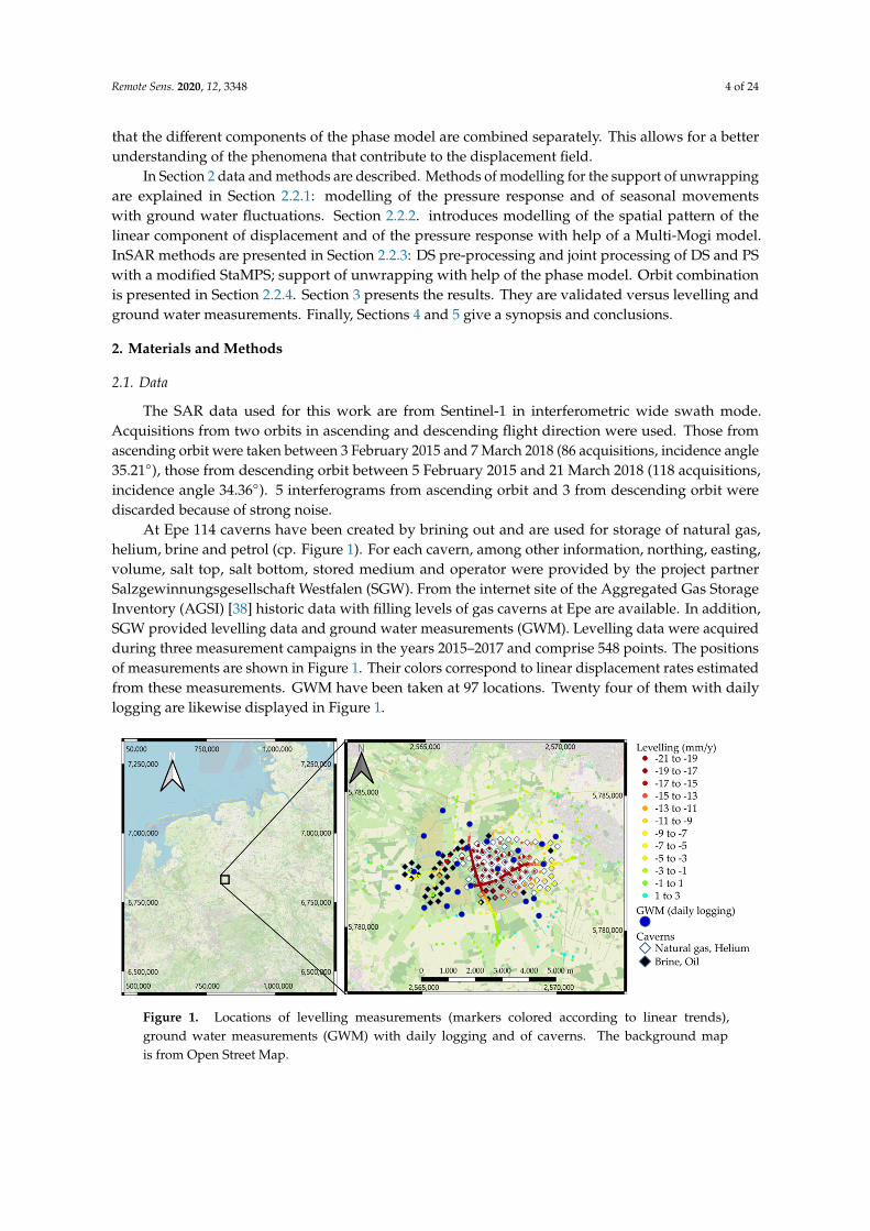
At Epe 114 caverns have been created by brining out and are used for storage of natural gas,helium, brine and petrol (cp. Figure 1). For each cavern, among other information, northing, easting,volume, salt top, salt bottom, stored medium and operator were provided by the project partnerSalzgewinnungsgesellschaft Westfalen (SGW). From the internet site of the Aggregated Gas StorageInventory (AGSI) [38] historic data with filling levels of gas caverns at Epe are available. In addition,SGW provided levelling data and ground water measurements (GWM). Levelling data were acquiredduring three measurement campaigns in the years 2015–2017 and comprise 548 points. The positionsof measurements are shown in Figure 1. Their colors correspond to linear displacement rates estimatedfrom these measurements. GWM have been taken at 97 locations. Twenty four of them with dailylogging are likewise displayed in Figure 1.

Remote Sens. 2020, 12, x FOR PEER REVIEW 4 of 24

this study is that the different components of the phase model are combined separately. This allows for a better understanding of the phenomena that contribute to the displacement field.

In Section 2 data and methods are described. Methods of modelling for the support of unwrapping are explained in Section 2.2.1: modelling of the pressure response and of seasonal movements with ground water fluctuations. Section 2.2.2. introduces modelling of the spatial pattern of the linear component of displacement and of the pressure response with help of a Multi-Mogi model. InSAR methods are presented in Section 2.2.3: DS pre-processing and joint processing of DS and PS with a modified StaMPS; support of unwrapping with help of the phase model. Orbit combination is presented in Section 2.2.4. Section 3 presents the results. They are validated versus levelling and ground water measurements. Finally, Sections 4 and 5 give a synopsis and conclusions.

2. Materials and Methods

2.1. Data

The SAR data used for this work are from Sentinel-1 in interferometric wide swath mode. Acquisitions from two orbits in ascending and descending flight direction were used. Those from ascending orbit were taken between 3 February 2015 and 7 March 2018 (86 acquisitions, incidence angle 35.21°), those from descending orbit between 5 February 2015 and 21 March 2018 (118 acquisitions, incidence angle 34.36°). 5 interferograms from ascending orbit and 3 from descending orbit were discarded because of strong noise.

At Epe 114 caverns have been created by brining out and are used for storage of natural gas, helium, brine and petrol (cp. Figure 1). For each cavern, among other information, northing, easting, volume, salt top, salt bottom, stored medium and operator were provided by the project partner Salzgewinnungsgesellschaft Westfalen (SGW). From the internet site of the Aggregated Gas Storage Inventory (AGSI) [38] historic data with filling levels of gas caverns at Epe are available. In addition, SGW provided levelling data and ground water measurements (GWM). Levelling data were acquired during three measurement campaigns in the years 2015–2017 and comprise 548 points. The positions of measurements are shown in Figure 1. Their colors correspond to linear displacement rates estimated from these measurements. GWM have been taken at 97 locations. Twenty four of them with daily logging are likewise displayed in Figure 1.

Figure 1. Locations of levelling measurements (markers colored according to linear trends), ground water measurements (GWM) with daily logging and of caverns. The background map is from Open Street Map.

Figure 1. Locations of levelling measurements (markers colored according to linear trends),ground water measurements (GWM) with daily logging and of caverns. The background mapis from Open Street Map.

Remote Sens. 2020, 12, 3348 5 of 24

2.2. Methodology

Modelling was used for two purposes. First, modelling was used to enhance unwrapping.Significant gradients of the displacement posed a challenge to the unwrapping algorithm of StaMPSand lead to unsatisfactory results. To improve on this, unwrapping was supported by use of a 3Dphase model (Section 2.2.1). Second, modelling the spatial displacement pattern helped to obtainmore accurate results from orbit combination. To this end, a model comprising multiple Mogi sourcesin elastic half-space was established in order to describe the spatial pattern of surface movements.With its help, LOS observations of linear convergence and of pressure response from both orbitscould be combined resulting in a more accurate estimation of vertical displacement than with apointwise calculation of vertical and east-west component of displacement. The model is introducedin Section 2.2.2 and its use for orbit combination is explained in Section 2.2.4.

2.2.1. Modelling for Support of Unwrapping

Because of significant temporal gradients of the observed displacement, unwrapping wassupported by use of a 3D phase model. The basis for the model is the observation that displacementabove the deposit has three main components: 1. linear subsidence caused by convergence of thecaverns; 2. pronounced nonlinear movement in response to pressure changes due to the injectionand withdrawal of gas; 3. seasonal displacement in peat areas due to water level changes. For eachpixel the coefficients of a linear combination of the three components are estimated from the data.For the pressure response and the seasonal movement temporal models were gained from preliminaryInSAR results and in case of the pressure response also geophysical considerations. The proceeding isdescribed below. Details on the algorithmic use are given in Section 2.2.3.

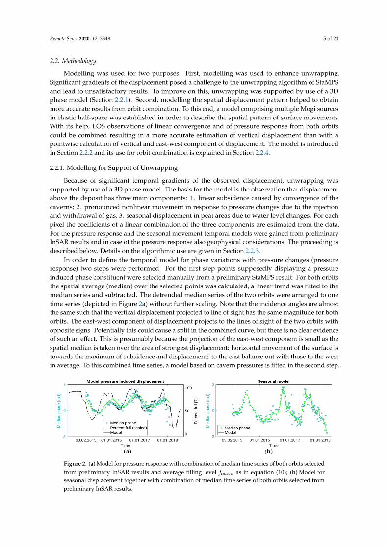
In order to define the temporal model for phase variations with pressure changes (pressureresponse) two steps were performed. For the first step points supposedly displaying a pressureinduced phase constituent were selected manually from a preliminary StaMPS result. For both orbitsthe spatial average (median) over the selected points was calculated, a linear trend was fitted to themedian series and subtracted. The detrended median series of the two orbits were arranged to onetime series (depicted in Figure 2a) without further scaling. Note that the incidence angles are almostthe same such that the vertical displacement projected to line of sight has the same magnitude for bothorbits. The east-west component of displacement projects to the lines of sight of the two orbits withopposite signs. Potentially this could cause a split in the combined curve, but there is no clear evidenceof such an effect. This is presumably because the projection of the east-west component is small as thespatial median is taken over the area of strongest displacement: horizontal movement of the surface istowards the maximum of subsidence and displacements to the east balance out with those to the westin average. To this combined time series, a model based on cavern pressures is fitted in the second step.


2.2. Methodology

Modelling was used for two purposes. First, modelling was used to enhance unwrapping. Significant gradients of the displacement posed a challenge to the unwrapping algorithm of StaMPS and lead to unsatisfactory results. To improve on this, unwrapping was supported by use of a 3D phase model (Section 2.2.1). Second, modelling the spatial displacement pattern helped to obtain more accurate results from orbit combination. To this end, a model comprising multiple Mogi sources in elastic half-space was established in order to describe the spatial pattern of surface movements. With its help, LOS observations of linear convergence and of pressure response from both orbits could be combined resulting in a more accurate estimation of vertical displacement than with a pointwise calculation of vertical and east-west component of displacement. The model is introduced in Section 2.2.2 and its use for orbit combination is explained in Section 2.2.4.

2.2.1. Modelling for Support of Unwrapping

Because of significant temporal gradients of the observed displacement, unwrapping was supported by use of a 3D phase model. The basis for the model is the observation that displacement above the deposit has three main components: 1. linear subsidence caused by convergence of the caverns; 2. pronounced nonlinear movement in response to pressure changes due to the injection and withdrawal of gas; 3. seasonal displacement in peat areas due to water level changes. For each pixel the coefficients of a linear combination of the three components are estimated from the data. For the pressure response and the seasonal movement temporal models were gained from preliminary InSAR results and in case of the pressure response also geophysical considerations. The proceeding is described below. Details on the algorithmic use are given in Section 2.2.3.

In order to define the temporal model for phase variations with pressure changes (pressure response) two steps were performed. For the first step points supposedly displaying a pressure induced phase constituent were selected manually from a preliminary StaMPS result. For both orbits the spatial average (median) over the selected points was calculated, a linear trend was fitted to the median series and subtracted. The detrended median series of the two orbits were arranged to one time series (depicted in Figure 2a) without further scaling. Note that the incidence angles are almost the same such that the vertical displacement projected to line of sight has the same magnitude for both orbits. The east-west component of displacement projects to the lines of sight of the two orbits with opposite signs. Potentially this could cause a split in the combined curve, but there is no clear evidence of such an effect. This is presumably because the projection of the east-west component is small as the spatial median is taken over the area of strongest displacement: horizontal movement of the surface is towards the maximum of subsidence and displacements to the east balance out with those to the west in average. To this combined time series, a model based on cavern pressures is fitted in the second step.

(a)

(b)

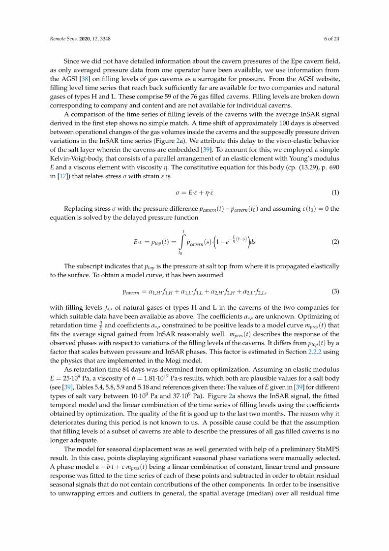
Figure 2. (a) Model for pressure response with combination of median time series of both orbits selected from preliminary InSAR results and average filling level 𝑓 as in equation (10); (b) Model for seasonal displacement together with combination of median time series of both orbits selected from preliminary InSAR results.

Figure 2. (a) Model for pressure response with combination of median time series of both orbits selectedfrom preliminary InSAR results and average filling level fcavern as in equation (10); (b) Model forseasonal displacement together with combination of median time series of both orbits selected frompreliminary InSAR results.

Remote Sens. 2020, 12, 3348 6 of 24

Since we did not have detailed information about the cavern pressures of the Epe cavern field,as only averaged pressure data from one operator have been available, we use information fromthe AGSI [38] on filling levels of gas caverns as a surrogate for pressure. From the AGSI website,filling level time series that reach back sufficiently far are available for two companies and naturalgases of types H and L. These comprise 59 of the 76 gas filled caverns. Filling levels are broken downcorresponding to company and content and are not available for individual caverns.

A comparison of the time series of filling levels of the caverns with the average InSAR signalderived in the first step shows no simple match. A time shift of approximately 100 days is observedbetween operational changes of the gas volumes inside the caverns and the supposedly pressure drivenvariations in the InSAR time series (Figure 2a). We attribute this delay to the visco-elastic behaviorof the salt layer wherein the caverns are embedded [39]. To account for this, we employed a simpleKelvin-Voigt-body, that consists of a parallel arrangement of an elastic element with Young’s modulusE and a viscous element with viscosity η. The constitutive equation for this body (cp. (13.29), p. 690in [17]) that relates stress σ with strain ε is

σ = E·ε+ η·.ε (1)

Replacing stress σ with the pressure difference pcavern(t) − pcavern(t0) and assuming ε(t0) = 0 theequation is solved by the delayed pressure function

E·ε = ptop(t) =

t∫t0

.pcavern(s)·

(1− e−

Eη (t−s)

)ds (2)

The subscript indicates that ptop is the pressure at salt top from where it is propagated elasticallyto the surface. To obtain a model curve, it has been assumed

pcavern = α1,H· f1,H + α1,L· f1,L + α2,H· f2,H + α2,L· f2,L, (3)

with filling levels f∗,∗ of natural gases of types H and L in the caverns of the two companies forwhich suitable data have been available as above. The coefficients α∗,∗ are unknown. Optimizing ofretardation time η

E and coefficients α∗,∗ constrained to be positive leads to a model curve mpres(t) thatfits the average signal gained from InSAR reasonably well. mpres(t) describes the response of theobserved phases with respect to variations of the filling levels of the caverns. It differs from ptop(t) by afactor that scales between pressure and InSAR phases. This factor is estimated in Section 2.2.2 usingthe physics that are implemented in the Mogi model.

As retardation time 84 days was determined from optimization. Assuming an elastic modulusE = 25·109 Pa, a viscosity of η = 1.81·1017 Pa·s results, which both are plausible values for a salt body(see [39], Tables 5.4, 5.8, 5.9 and 5.18 and references given there; The values of E given in [39] for differenttypes of salt vary between 10·109 Pa and 37·109 Pa). Figure 2a shows the InSAR signal, the fittedtemporal model and the linear combination of the time series of filling levels using the coefficientsobtained by optimization. The quality of the fit is good up to the last two months. The reason why itdeteriorates during this period is not known to us. A possible cause could be that the assumptionthat filling levels of a subset of caverns are able to describe the pressures of all gas filled caverns is nolonger adequate.

The model for seasonal displacement was as well generated with help of a preliminary StaMPSresult. In this case, points displaying significant seasonal phase variations were manually selected.A phase model a + b·t + c·mpres(t) being a linear combination of constant, linear trend and pressureresponse was fitted to the time series of each of these points and subtracted in order to obtain residualseasonal signals that do not contain contributions of the other components. In order to be insensitiveto unwrapping errors and outliers in general, the spatial average (median) over all residual time

Remote Sens. 2020, 12, 3348 7 of 24

series was calculated. That way average seasonal phase time series for both orbits were obtained.Combined, they form a new time series with values for all acquisition times of both orbits. This timeseries still contains some outliers caused by unwrapping errors in some interferograms that affectedwhole groups of points. Therefore, robust locally weighted quadratic regression (RLOESS) in a movingwindow of length 15 acquisitions was applied in order to prevent that the outliers influence themodel significantly. This means that inside the moving window a quadratic polynomial is fitted tothe time series using robust iterative reweighting. In order to preserve the pronounced shape of thesignal the regression was performed separately inside the four intervals defined by the three peaks.Figure 2b shows the InSAR signal and the fitted seasonal model.

It has to be remarked, that we did not use observed time series of groundwater measurements tomodel the seasonal phase constituent. The reason is that well level variations are often representativefor local areas only, and even well levels in immediate vicinity may give significantly differing results.Additionally, a time delay between the response of the surface layers to water input and the waterlevel of a certain well has to be expected. To account for that, diffusion models should have beenimplemented. We did not do this because we don’t have enough information about the governinghydraulic parameters that are supposed to exhibit strong spatial variations. In Section 3.1, we compareINSAR-derived seasonal displacements over a fen in the western part of the cavern field with waterlevel variations of the surrounding wells (cf. Figure 1). Although the levels partly show markeddifferences to our seasonal model, the general agreement is good which indicates that the modelis plausible.

2.2.2. Modelling Used for Orbit Combination

For orbit combination, a simplistic model for the spatial pattern of surface displacements isemployed that will be called Multi-Mogi model in this paper. It assumes that each cavern is surroundedby a spherical salt mantel with a thickness of 75 m. The uppermost point of the salt sphere coincideswith top salt at the position of a certain cavern. The salt spheres act as pressure or volume sourcesembedded in an elastic halfspace, often called “Mogi” sources in honor of [37]. The pressure at theoutside of the salt spheres is given by ptop(t), which is related to the pressure variation in the interior ofthe caverns according to equations (1) and (2). Thus, the model employs an elastic part, governed bythe Mogi approach, and a visco-elastic component governed by the Kelvin-Voigt body. We furtherassume that the surface deformation pattern results from the linear superposition of the contributionsof each cavern. For simplicity, we use the term “cavern” to denote the composite pressure source inthe following.

The elastic contribution of a cavern situated at (xc, yc) in depth dc at coordinates (x, y) to surfacedisplacement is proportional to

Mc(x, y) =2(1− ν2

)a3

c

E

(x− xc)/R3

(y− yc)/R3

dc/R3

, (4)

where E is the elastic module and ν is the Poisson ratio in the elastic halfspace,

R =

√(x− xc)

2 + (y− yc)2 + dc2 (5)

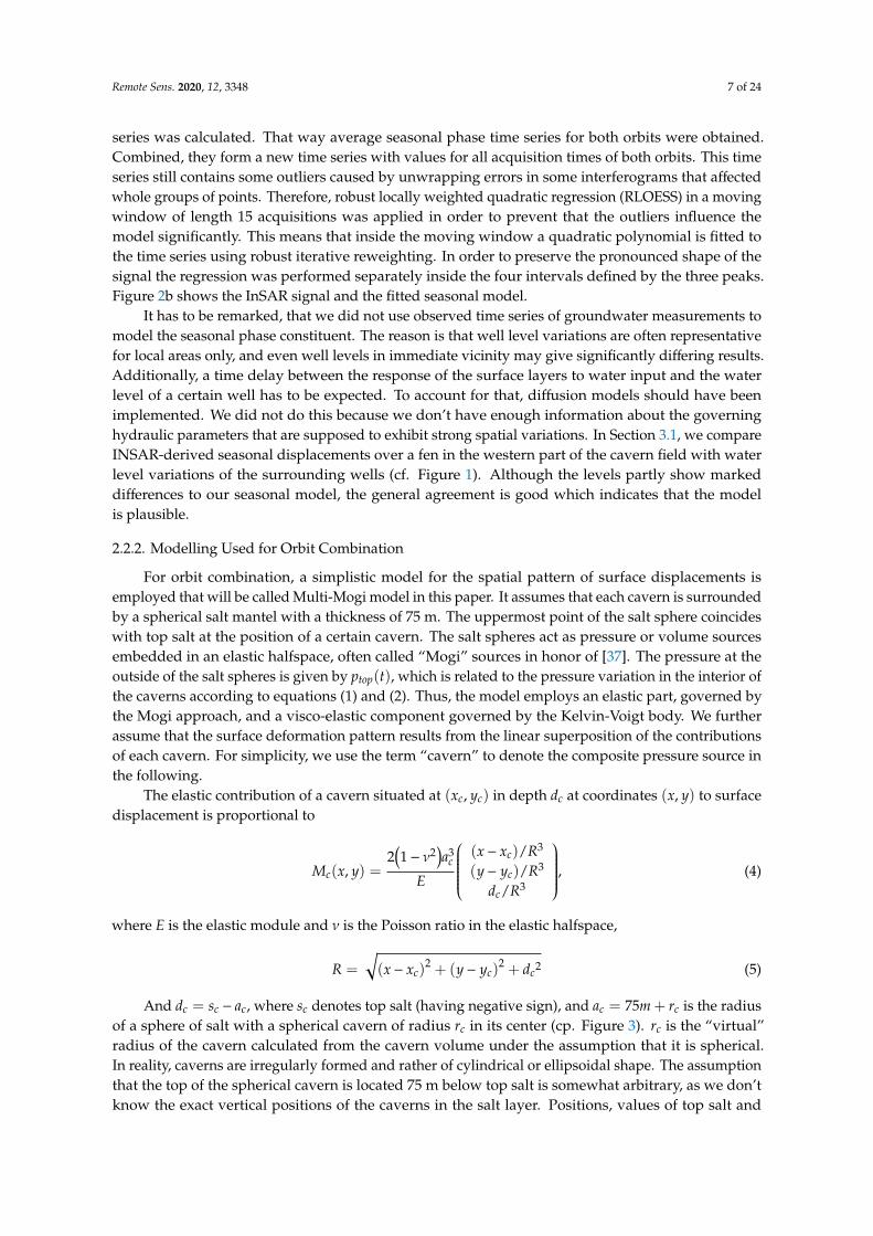
And dc = sc − ac, where sc denotes top salt (having negative sign), and ac = 75m + rc is the radiusof a sphere of salt with a spherical cavern of radius rc in its center (cp. Figure 3). rc is the “virtual”radius of the cavern calculated from the cavern volume under the assumption that it is spherical.In reality, caverns are irregularly formed and rather of cylindrical or ellipsoidal shape. The assumptionthat the top of the spherical cavern is located 75 m below top salt is somewhat arbitrary, as we don’tknow the exact vertical positions of the caverns in the salt layer. Positions, values of top salt and

Remote Sens. 2020, 12, 3348 8 of 24

volumes of the caverns were provided by the project partners. For the elastic half space an elasticmodulus E = 30·109 Pa and a Poisson ration ν = 0.25 have been chosen, because values for the caprock at Epe are not known to us. As a consequence of the big diversity of values of E for cap rock,this number is even less reliable as that assumed for the salt. As a final remark, it should be pointedout that the uncertainty regarding the assumed values of Young’s modulus E has no influence onthe results from InSAR as they always occur as E times estimated parameter, where the estimatedparameter is not interpreted on its own. The Mogi model is used here to describe two components ofthe displacement field: either for the parameters of the linear component of the displacement model orof the pressure response. In the case of the linear component it is assumed that all caverns convergewith the same rate. This means only one parameter plin is assumed to be unknown (describing volumechange with time t) and has to be determined such that the projections to LOS of the displacement

Dlin(x, y, t) = t·plin·∑c∈C

Mc(x, y) (6)

approximate optimally the linear model component for both orbits and all points found by InSARprocessing (C denotes the set of all caverns). According to the Mogi [37] formalism, plin is related to acontinuous volume loss Vlin of the spherical pressure source:

plin =Vlin·E

a3c ·π·2(1 + ν)

(7)


that all caverns converge with the same rate. This means only one parameter 𝑝 is assumed to be unknown (describing volume change with time 𝑡) and has to be determined such that the projections to LOS of the displacement 𝐷 𝑥, 𝑦, 𝑡 = 𝑡 ∙ 𝑝 ∙ 𝑀 𝑥, 𝑦∈ (6)

approximate optimally the linear model component for both orbits and all points found by InSAR processing (𝐶 denotes the set of all caverns). According to the Mogi [37] formalism, 𝑝 is related to a continuous volume loss 𝑉 of the spherical pressure source: 𝑝 = 𝑉 ∙ 𝐸𝑎 ∙ 𝜋 ∙ 2 1 + 𝜈 (7)

Optimization gives annual volumetric convergence rates of the order of 1%, which are quite realistic.

Figure 3. Sketch of the geometric arrangement of a cavern as used for modelling (𝑑 depth of cavern center, 𝑠 top salt, 𝑎 radius of salt sphere, 𝑟 cavern radius). In case of the pressure response, only gas containing caverns are assumed to contribute and

displacement is proportional to the pressure on the surface of the salt sphere, which is obtained from cavern pressure according to Equation (2). The pressure in all these caverns is assumed to be the same at all times. Displacement at coordinates 𝑥, 𝑦 at time 𝑡 as described by the Multi-Mogi model is obtained as 𝐷 𝑥, 𝑦, 𝑡 = 𝑝 𝑡 ∙ 𝑀 𝑥, 𝑦∈ = 𝑚 𝑡 ∙ 𝑝 ∙ 𝑀 𝑥, 𝑦∈ (8)

As above 𝑚 is the model for the pressure response and 𝐶 𝑝𝑟𝑒𝑠 denotes the set of all gas filled caverns. The parameter 𝑝 is determined such that the projections to LOS of 𝐷 approximate optimally the component of the pressure response for both orbits and all points found by InSAR processing.

The parameter 𝑝 estimated for the pressure response allows to guess the difference ∆𝑃 of the maximal cavern pressure to the pressure 𝑃 corresponding to filling level zero (unknown to us). To this end we calculate the pressure difference

Figure 3. Sketch of the geometric arrangement of a cavern as used for modelling (dc depth of caverncenter, sc top salt, ac radius of salt sphere, rc cavern radius).

Optimization gives annual volumetric convergence rates of the order of 1%, which are quite realistic.In case of the pressure response, only gas containing caverns are assumed to contribute and

displacement is proportional to the pressure on the surface of the salt sphere, which is obtained fromcavern pressure according to Equation (2). The pressure in all these caverns is assumed to be the sameat all times. Displacement at coordinates (x, y) at time t as described by the Multi-Mogi model isobtained as

Dpres(x, y, t) = ptop(t)·∑

c∈C(pres)

Mc(x, y) = mpres(t)·ppres·∑

c∈C(pres)

Mc(x, y) (8)

Remote Sens. 2020, 12, 3348 9 of 24

As above mpres is the model for the pressure response and C(pres) denotes the set of allgas filled caverns. The parameter ppres is determined such that the projections to LOS of Dpres

approximate optimally the component of the pressure response for both orbits and all points found byInSAR processing.

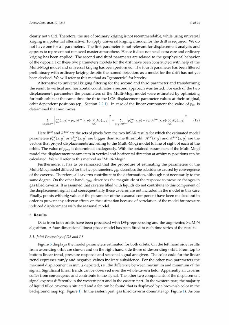
The parameter ppres estimated for the pressure response allows to guess the difference ∆Pmax ofthe maximal cavern pressure to the pressure P0 corresponding to filling level zero (unknown to us).To this end we calculate the pressure difference

∆ptop = ptop(tmax) − ptop(tmin) = ppres·(mpres(tmax) −mpres(tmin)

)(9)

effecting elastically the maximal displacement [37], i.e., the difference between maximum and minimumof the displacement signal. The cavern pressure is proportional to the amount of gas in the cavernaccording to the Van der Waals equation for constant temperature. Temperatures in the depth of thecaverns can be assumed to be constant on average. If it is assumed that the weighted average fcavern

of known filling levels (with sum of weights equal one) is a good approximation of the actual fillinglevels, then the cavern pressure can be expressed as

pcavern = ∆Pmax· fcavern + P0 = ∆Pmax·α1,H· f1,H + α1,L· f1,L + α2,H· f2,H + α2,L· f2,L

α1,H + α1,L + α2,H + α2,L+ P0 (10)

and the left-hand side of Equation (9) can be calculated by evaluating Equation (2) at tmax and tmin:

∆ptop = ∆Pmax·

tmax∫t0

.f cavern(s)·

(1− e−

Eη (t−s)

)ds−

tmin∫t0

.f cavern(s)·

(1− e−

Eη (t−s)

)ds

(11)

From (9) and (11) the guess of ∆Pmax can be calculated. Anticipating the result, ∆Pmax = 5.3·106 Pa isobtained, which probably is at the lower end of the real pressure values. Nevertheless, the order ofmagnitude is reasonable which indicates that the simplistic model is physically plausible.

2.2.3. InSAR Methodology

The InSAR processing runs through three principal steps: 1. Coregistration and interferogramformation with ESAs Sentinel-1 Toolbox; 2. DS pre-processing following the paradigm of SqueeSAR;3. Joint processing of DS and PS with a modified and augmented version of StaMPS 3.3b1.Coregistration and interferogram formation are standard Sentinel Application Platform (SNAP)functionality and are not further discussed here.

In order to jointly process DS and PS with StaMPS two principal algorithmic changes have beenperformed: 1. The introduction of DS pre-processing as a new component, which estimates for eachpixel a complex signal that in case of good quality can be used like that of a PS in an arbitrary PSalgorithm. 2. The modification of the pixel selection step of StaMPS, where is decided which pointsare kept for further processing. This comprises assessing the quality of DS and PS signals and alsodeciding if the DS or PS signal shall be used in case both are of good quality.

The basic concept for pre-processing of DS stems from the SqueeSAR paper [18] and consists ofgrouping for each pixel a statistical homogeneous neighborhood, estimating the covariance matrixand DS signal estimation. Since the introduction of SqueeSAR, a multitude of approaches has beendeveloped to perform these tasks e.g., [40–46], for a review see [19]. For the results presented in thiswork the following methods were applied: The approach of [44] was used for the grouping step.It consists of signal transformation, outlier removal based on the adjusted boxplot, and application ofthe one-sample t-test. The one-sample t-test was applied with significance level 0.99. From each pixelin the neighborhood up to eight outliers were allowed to be removed (the investigated stacks comprise86 and 118 acquisitions). Pixels with more outliers were discarded. The covariance was estimated as a

Remote Sens. 2020, 12, 3348 10 of 24

3D-version of the sample covariance matrix (outlying values are set to zero). The square roots of itsdiagonal values serve as amplitudes of the DS signal. The phases of the DS signal were estimated withphase triangulation coherence maximization [19,47], which is for small neighborhoods more reliablethan the maximum likelihood estimator derived in [48].

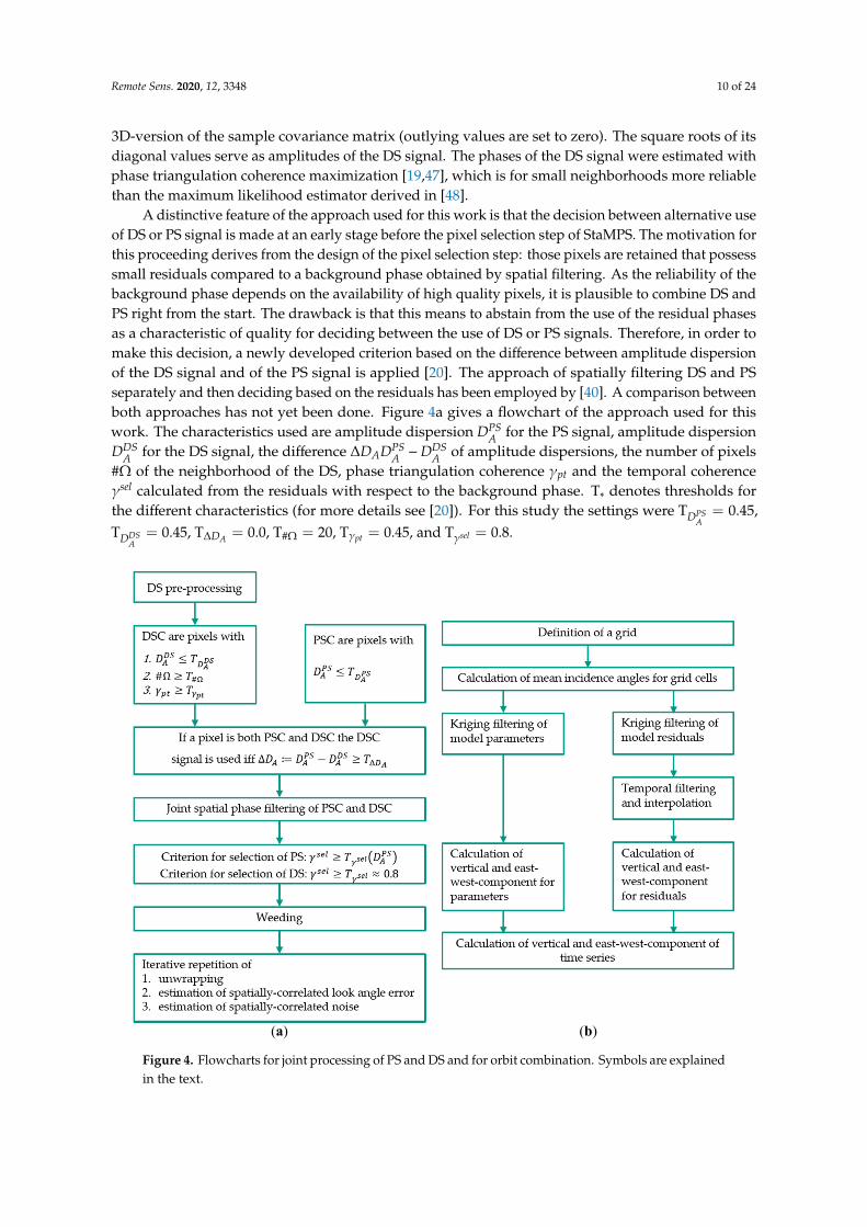
A distinctive feature of the approach used for this work is that the decision between alternative useof DS or PS signal is made at an early stage before the pixel selection step of StaMPS. The motivation forthis proceeding derives from the design of the pixel selection step: those pixels are retained that possesssmall residuals compared to a background phase obtained by spatial filtering. As the reliability of thebackground phase depends on the availability of high quality pixels, it is plausible to combine DS andPS right from the start. The drawback is that this means to abstain from the use of the residual phasesas a characteristic of quality for deciding between the use of DS or PS signals. Therefore, in order tomake this decision, a newly developed criterion based on the difference between amplitude dispersionof the DS signal and of the PS signal is applied [20]. The approach of spatially filtering DS and PSseparately and then deciding based on the residuals has been employed by [40]. A comparison betweenboth approaches has not yet been done. Figure 4a gives a flowchart of the approach used for thiswork. The characteristics used are amplitude dispersion DPS

A for the PS signal, amplitude dispersionDDS

A for the DS signal, the difference ∆DADPSA −DDS

A of amplitude dispersions, the number of pixels#Ω of the neighborhood of the DS, phase triangulation coherence γpt and the temporal coherenceγsel calculated from the residuals with respect to the background phase. T∗ denotes thresholds forthe different characteristics (for more details see [20]). For this study the settings were TDPS

A= 0.45,

TDDSA

= 0.45, T∆DA = 0.0, T#Ω = 20, Tγpt = 0.45, and Tγsel = 0.8.


signals. Therefore, in order to make this decision, a newly developed criterion based on the difference between amplitude dispersion of the DS signal and of the PS signal is applied [20]. The approach of spatially filtering DS and PS separately and then deciding based on the residuals has been employed by [40]. A comparison between both approaches has not yet been done. Figure 4a gives a flowchart of the approach used for this work. The characteristics used are amplitude dispersion 𝐷 for the PS signal, amplitude dispersion 𝐷 for the DS signal, the difference 𝛥𝐷 ≔ 𝐷 − 𝐷 of amplitude dispersions, the number of pixels #Ω of the neighborhood of the DS, phase triangulation coherence 𝛾 and the temporal coherence 𝛾 calculated from the residuals with respect to the background phase. T∗ denotes thresholds for the different characteristics (for more details see [20]). For this study the settings were T = 0.45, T = 0.45, T = 0.0, T# = 20, T = 0.45, and T = 0.8.

(a) (b)

Figure 4. Flowcharts for joint processing of PS and DS and for orbit combination. Symbols are explained in the text.

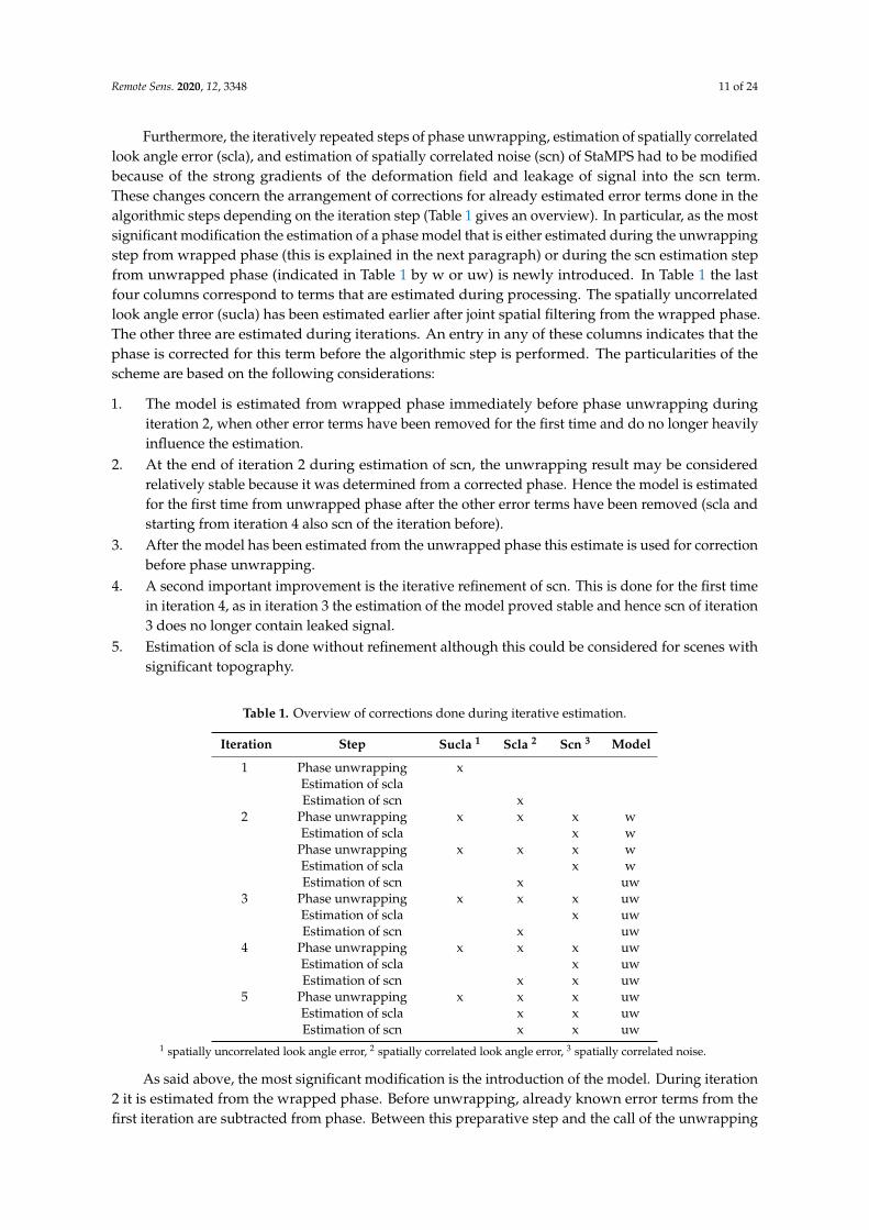
Furthermore, the iteratively repeated steps of phase unwrapping, estimation of spatially correlated look angle error (scla), and estimation of spatially correlated noise (scn) of StaMPS had to be modified because of the strong gradients of the deformation field and leakage of signal into the scn term. These changes concern the arrangement of corrections for already estimated error terms done in the algorithmic steps depending on the iteration step (Table 1 gives an overview). In particular, as the most significant modification the estimation of a phase model that is either estimated during the unwrapping step from wrapped phase (this is explained in the next paragraph) or during the scn estimation step from unwrapped phase (indicated in Table 1 by w or uw) is newly introduced. In Table 1 the last four columns correspond to terms that are estimated during processing. The spatially uncorrelated look angle error (sucla) has been estimated earlier after joint spatial filtering from the wrapped phase. The other three are estimated during iterations. An entry in any of these columns indicates that the phase is corrected for this term before the algorithmic step is performed. The particularities of the scheme are based on the following considerations:

Figure 4. Flowcharts for joint processing of PS and DS and for orbit combination. Symbols are explainedin the text.

Remote Sens. 2020, 12, 3348 11 of 24

Furthermore, the iteratively repeated steps of phase unwrapping, estimation of spatially correlatedlook angle error (scla), and estimation of spatially correlated noise (scn) of StaMPS had to be modifiedbecause of the strong gradients of the deformation field and leakage of signal into the scn term.These changes concern the arrangement of corrections for already estimated error terms done in thealgorithmic steps depending on the iteration step (Table 1 gives an overview). In particular, as the mostsignificant modification the estimation of a phase model that is either estimated during the unwrappingstep from wrapped phase (this is explained in the next paragraph) or during the scn estimation stepfrom unwrapped phase (indicated in Table 1 by w or uw) is newly introduced. In Table 1 the lastfour columns correspond to terms that are estimated during processing. The spatially uncorrelatedlook angle error (sucla) has been estimated earlier after joint spatial filtering from the wrapped phase.The other three are estimated during iterations. An entry in any of these columns indicates that thephase is corrected for this term before the algorithmic step is performed. The particularities of thescheme are based on the following considerations:

1. The model is estimated from wrapped phase immediately before phase unwrapping duringiteration 2, when other error terms have been removed for the first time and do no longer heavilyinfluence the estimation.

2. At the end of iteration 2 during estimation of scn, the unwrapping result may be consideredrelatively stable because it was determined from a corrected phase. Hence the model is estimatedfor the first time from unwrapped phase after the other error terms have been removed (scla andstarting from iteration 4 also scn of the iteration before).

3. After the model has been estimated from the unwrapped phase this estimate is used for correctionbefore phase unwrapping.

4. A second important improvement is the iterative refinement of scn. This is done for the first timein iteration 4, as in iteration 3 the estimation of the model proved stable and hence scn of iteration3 does no longer contain leaked signal.

5. Estimation of scla is done without refinement although this could be considered for scenes withsignificant topography.

Table 1. Overview of corrections done during iterative estimation.

Iteration Step Sucla 1 Scla 2 Scn 3 Model

1 Phase unwrapping xEstimation of sclaEstimation of scn x

2 Phase unwrapping x x x wEstimation of scla x w

Phase unwrapping x x x wEstimation of scla x wEstimation of scn x uw

3 Phase unwrapping x x x uwEstimation of scla x uwEstimation of scn x uw

4 Phase unwrapping x x x uwEstimation of scla x uwEstimation of scn x x uw

5 Phase unwrapping x x x uwEstimation of scla x x uwEstimation of scn x x uw

1 spatially uncorrelated look angle error, 2 spatially correlated look angle error, 3 spatially correlated noise.

As said above, the most significant modification is the introduction of the model. During iteration2 it is estimated from the wrapped phase. Before unwrapping, already known error terms from thefirst iteration are subtracted from phase. Between this preparative step and the call of the unwrapping

Remote Sens. 2020, 12, 3348 12 of 24

algorithm, this estimation step has been newly inserted. It performs a parameter space search for aphase model. Those parameters are selected which maximize the temporal coherence of the residuals.The phase model for the gas deposit assumes a linear combination of linear trend, pressure responseand seasonal movement and is subtracted from the wrapped phase before unwrapping starts. After theunwrapping algorithm has terminated, the modeled phase is added to its result.

In order to make this step reliable several improvements have been added:

1. As the runtime of a parameter space search increases exponentially with its dimension the modelparameters are only determined for the points inside a window that has been defined beforehand.

2. In order to avoid unwrapping problems near the window frame a smooth transition between themodelled phase in the inside and zero on the outside is enforced.

3. To prevent that badly estimated parameters influence unwrapping negatively, the parameters arespatially filtered.

4. Spatially correlated noise generally will be significant during early iterations. Therefore,a sub-window has been defined, that serves as reference area. The mean phase of the points inthis window are subtracted from wrapped phase before the model parameters are determined.

2.2.4. Orbit Combination

As DS and PS lie scattered and do not coincide for different orbits the two outputs of StaMPShave to be interpolated to common positions for the purpose of orbit combination. Likewise, times ofacquisition do not agree, which makes temporal interpolation necessary. Unfortunately, interpolationand filtering tend to attenuate the estimated signal, particularly in the presence of noise. In thissituation, the a priori knowledge about the deformation process that is reflected in the Multi-Mogimodel described in Section 2.2.2 might potentially be used to preserve better the underlying signal.Hence orbit combination was implemented in two ways that are explained in the sequel. Before doingso, the principal steps of orbit combination are described:

1. Definition of a grid to which values shall be interpolated (Gauß-Krüger coordinates and cells of100 m times 100 m were used). As it makes sense to process only grid cells that contain pointsfrom both orbits their size has been chosen in a way that almost all points fall in such relevantgrid cells.

2. For each grid cell and both orbits a mean incidence angle was calculated by averaging over thevalues for the points lying in the cell.

3. Kriging filtering [49] is used to interpolate for each acquisition and orbit the values of thedisplacement time series to the relevant grid cells.

4. Time series of each orbit were filtered with robust quadratic regression in a moving window (oflength 9 acquisitions) to remove any outliers left. Acquisitions outside the overlap of the twoseries were discarded. The period between 5 February 2015 and 21 December 2017 remained.

5. The linear equation system for orbit combination for each point and using the interpolated timeseries was solved in an analogous way as was done by [50].

This basic version of orbit combination uses the displacement time series from StaMPS. In orderto generate the results in the next section, a more complex approach has been adopted (Figure 4b givesa flowchart). A parametric linear model consisting of constant, linear trend, pressure response andseasonal movement was fitted to the displacement time series. This way they were split in a modeledpart and an unmodeled residual. Steps 3 to 5 were modified accordingly: (a) for the unmodeledresidual they have been performed as before; (b) for the modeled part kriging filtering has been appliedto the parameters and the transformation from LOS to vertical and east-west component has beenperformed separately for them, which has the advantage to preserve the decomposition in the differentcomponents thus allowing to investigate them separately. The algorithm used for kriging filtering ofthe parameters is different for two of them. For all parameters the assumption of a constant drift is

Remote Sens. 2020, 12, 3348 13 of 24

clearly not valid. Therefore, the use of ordinary kriging is not recommendable, while using universalkriging is a potential alternative. To apply universal kriging a model for the drift is required. We donot have one for all parameters. The first parameter is not relevant for displacement analysis andappears to represent not removed master atmosphere. Hence it does not need extra care and ordinarykriging has been applied. The second and third parameter are related to the geophysical behaviorof the deposit. For these two parameters models for the drift have been constructed with help of theMulti-Mogi model and universal kriging has been performed. The fourth parameter has been filteredpreliminary with ordinary kriging despite the named objection, as a model for the drift has not yetbeen devised. We will refer to this method as “geometric” for brevity.

Alternative to universal kriging filtering for the second and third parameter and transformingthe result to vertical and horizontal coordinates a second approach was tested. For each of the twodisplacement parameters the parameters of the Multi-Mogi model were estimated by optimizingfor both orbits at the same time the fit to the LOS displacement parameter values at their original,orbit dependent positions (cp. Section 2.2.1). In case of the linear component the value of plin isdetermined that minimizes

∑(x,y)∈Rasc

∣∣∣∣∣∣pasclin (x, y) − plin·Aasc(x, y)·

∑c∈C

Mc(x, y)

∣∣∣∣∣∣2 + ∑(x,y)∈Rdesc

∣∣∣∣∣∣pdesclin (x, y) − plin·Adesc(x, y)·

∑c∈C

Mc(x, y)

∣∣∣∣∣∣2 (12)

Here Rasc and Rdesc are the sets of pixels from the two InSAR results for which the estimated modelparameters pasc

lin (x, y) or pdesclin (x, y) are bigger than some threshold. Aasc(x, y) and Adesc(x, y) are the

vectors that project displacements according to the Multi-Mogi model to line of sight of each of theorbits. The value of ppres is determined analogously. With the obtained parameters of the Multi-Mogimodel the displacement parameters in vertical and horizontal direction at arbitrary positions can becalculated. We will refer to this method as “Multi-Mogi”.

Furthermore, it has to be remarked that the procedure of estimating the parameters of theMulti-Mogi model differed for the two parameters. plin describes the subsidence caused by convergenceof the caverns. Therefore, all caverns contribute to the deformation, although not necessarily to thesame degree. On the other hand, ppres describes the magnitude of the response to pressure changes ingas filled caverns. It is assumed that caverns filled with liquids do not contribute to this component ofthe displacement signal and consequentially these caverns are not included in the model in this case.Finally, points with big value of the parameter of the seasonal component have been masked out inorder to prevent any adverse effects on the estimation because of correlation of the model for pressureinduced displacement with the seasonal model.

3. Results

Data from both orbits have been processed with DS-preprocessing and the augmented StaMPSalgorithm. A four dimensional linear phase model has been fitted to each time series of the results.

3.1. Joint Processing of DS and PS

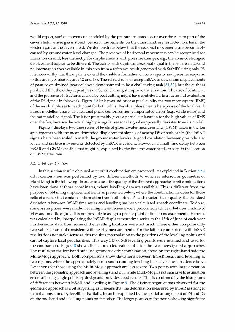
Figure 5 displays the model parameters estimated for both orbits. On the left hand side resultsfrom ascending orbit are shown and on the right hand side those of descending orbit. From top tobottom linear trend, pressure response and seasonal signal are given. The color code for the lineartrend expresses mm/y and negative values indicate subsidence. For the other two parameters themaximal displacement in mm is depicted, i.e., the difference between maximum and minimum of thesignal. Significant linear trends can be observed over the whole cavern field. Apparently all cavernssuffer from convergence and contribute to the signal. The other two components of the displacementsignal express differently in the western part and in the eastern part. In the western part, the majorityof liquid filled caverns is situated and a fen can be found that is displayed by a brownish color in thebackground map (cp. Figure 1). In the eastern part, gas filled caverns dominate (cp. Figure 1). As one

Remote Sens. 2020, 12, 3348 14 of 24

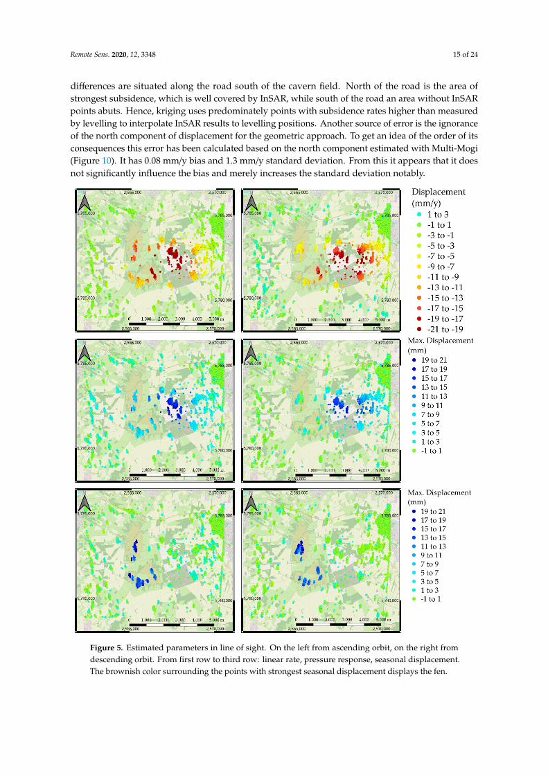
would expect, surface movements modeled by the pressure response occur over the eastern part of thecavern field, where gas is stored. Seasonal movements, on the other hand, are restricted to a fen in thewestern part of the cavern field. We demonstrate below that the seasonal movements are presumablycaused by groundwater level changes. The presence of horizontal movements can be recognized forlinear trends and, less distinctly, for displacements with pressure changes, e.g., the areas of strongestdisplacement appear to be different. The points with significant seasonal signal in the fen are all DS andno information was available in this area from a reference result generated with StaMPS using only PS.It is noteworthy that these points extend the usable information on convergence and pressure responseto this area (cp. also Figures 12 and 13). The related case of using InSAR to determine displacementsof pasture on drained peat soils was demonstrated to be a challenging task [51,52], but the authorspredicted that the 6-day repeat pass of Sentinel-1 might improve the situation. The use of Sentinel-1and the presence of structures caused by peat cutting might have contributed to a successful evaluationof the DS signals in this work. Figure 6 displays as indicator of pixel quality the root mean square (RMS)of the residual phases for each point for both orbits. Residual phase means here phase of the final resultminus modelled phase. The residual phase comprises non-compensated errors (e.g., white noise) andthe not modelled signal. The latter presumably gives a partial explanation for the high values of RMSover the fen, because the actual highly irregular seasonal signal supposedly deviates from its model.

Figure 7 displays two time series of levels of groundwater measurements (GWM) taken in the fenarea together with the mean detrended displacement signals of nearby DS of both orbits (the InSARsignals have been scaled to match the groundwater levels). A good correlation between groundwaterlevels and surface movements detected by InSAR is evident. However, a small time delay betweenInSAR and GWM is visible that might be explained by the time the water needs to seep to the locationof GWM after rain.

3.2. Orbit Combination

In this section results obtained after orbit combination are presented. As explained in Section 2.2.4orbit combination was performed by two different methods to which is referred as geometric orMulti-Mogi in the following. In order to assess the quality of the different approaches orbit combinationshave been done at those coordinates, where levelling data are available. This is different from thepurpose of obtaining displacement fields as presented below, where the combination is done for thosecells of a raster that contains information from both orbits. As a characteristic of quality the standarddeviation σ between InSAR time series and levelling has been calculated at each coordinate. To do so,some assumptions were made. Levelling measurements were performed each year between middle ofMay and middle of July. It is not possible to assign a precise point of time to measurements. Hence σ

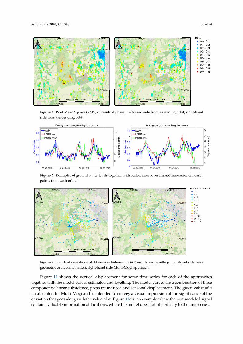
was calculated by interpolating the InSAR displacement time series to the 15th of June of each year.Furthermore, data from some of the levelling locations were not used. These either comprise onlytwo values or are not consistent with nearby measurements. For the latter a comparison with InSARresults does not make sense as this requires interpolation to the positions of the levelling points andcannot capture local peculiarities. This way 517 of 548 levelling points were retained and used forthe comparison. Figure 8 shows the color coded values of σ for the two investigated approaches.The results on the left-hand side use geometric orbit combination, those on the right-hand side theMulti-Mogi approach. Both comparisons show deviations between InSAR result and levelling attwo regions, where the approximately north-south running levelling line leaves the subsidence bowl.Deviations for those using the Multi-Mogi approach are less severe. Two points with large deviationbetween the geometric approach and levelling stand out, while Multi-Mogi is not sensitive to estimationerrors affecting single points by design and provides good results. This is confirmed by the histogramsof differences between InSAR and levelling in Figure 9. The distinct negative bias observed for thegeometric approach is a bit surprising as it means that the deformation measured by InSAR is strongerthan that measured by levelling. Partially, it can be explained by the spatial arrangement of PS and Dson the one hand and levelling points on the other. The larger portion of the points showing significant

Remote Sens. 2020, 12, 3348 15 of 24

differences are situated along the road south of the cavern field. North of the road is the area ofstrongest subsidence, which is well covered by InSAR, while south of the road an area without InSARpoints abuts. Hence, kriging uses predominately points with subsidence rates higher than measuredby levelling to interpolate InSAR results to levelling positions. Another source of error is the ignoranceof the north component of displacement for the geometric approach. To get an idea of the order of itsconsequences this error has been calculated based on the north component estimated with Multi-Mogi(Figure 10). It has 0.08 mm/y bias and 1.3 mm/y standard deviation. From this it appears that it doesnot significantly influence the bias and merely increases the standard deviation notably.


presumably gives a partial explanation for the high values of RMS over the fen, because the actual highly irregular seasonal signal supposedly deviates from its model.

Figure 5. Estimated parameters in line of sight. On the left from ascending orbit, on the right from descending orbit. From first row to third row: linear rate, pressure response, seasonal displacement. The brownish color surrounding the points with strongest seasonal displacement displays the fen.

Figure 5. Estimated parameters in line of sight. On the left from ascending orbit, on the right fromdescending orbit. From first row to third row: linear rate, pressure response, seasonal displacement.The brownish color surrounding the points with strongest seasonal displacement displays the fen.

Remote Sens. 2020, 12, 3348 16 of 24Remote Sens. 2020, 12, x FOR PEER REVIEW 15 of 24

Figure 6. Root Mean Square (RMS) of residual phase. Left-hand side from ascending orbit, right-hand side from descending orbit.

Figure 7 displays two time series of levels of groundwater measurements (GWM) taken in the fen area together with the mean detrended displacement signals of nearby DS of both orbits (the InSAR signals have been scaled to match the groundwater levels). A good correlation between groundwater levels and surface movements detected by InSAR is evident. However, a small time delay between InSAR and GWM is visible that might be explained by the time the water needs to seep to the location of GWM after rain.

Figure 7. Examples of ground water levels together with scaled mean over InSAR time series of nearby points from each orbit.


In this section results obtained after orbit combination are presented. As explained in Section 2.2.4 orbit combination was performed by two different methods to which is referred as geometric or Multi-Mogi in the following. In order to assess the quality of the different approaches orbit combinations have been done at those coordinates, where levelling data are available. This is different from the purpose of obtaining displacement fields as presented below, where the combination is done for those cells of a raster that contains information from both orbits. As a characteristic of quality the standard deviation σ between InSAR time series and levelling has been calculated at each coordinate. To do so, some assumptions were made. Levelling measurements were performed each year between middle of May and middle of July. It is not possible to assign a precise point of time to measurements. Hence σ was calculated by interpolating the InSAR displacement time series to the 15th of June of each year. Furthermore, data from some of the levelling locations were not used. These either comprise only two values or are not consistent with nearby measurements. For the latter a comparison with InSAR results does not make sense as this requires interpolation to the positions of the levelling points and cannot capture local peculiarities. This way 517 of 548 levelling points were retained and used for the comparison. Figure 8 shows the color coded values of σ for the two investigated approaches. The results on the left-hand side use geometric orbit combination, those on

Figure 6. Root Mean Square (RMS) of residual phase. Left-hand side from ascending orbit, right-handside from descending orbit.


Figure 6. Root Mean Square (RMS) of residual phase. Left-hand side from ascending orbit, right-hand side from descending orbit.

Figure 7 displays two time series of levels of groundwater measurements (GWM) taken in the fen area together with the mean detrended displacement signals of nearby DS of both orbits (the InSAR signals have been scaled to match the groundwater levels). A good correlation between groundwater levels and surface movements detected by InSAR is evident. However, a small time delay between InSAR and GWM is visible that might be explained by the time the water needs to seep to the location of GWM after rain.

Figure 7. Examples of ground water levels together with scaled mean over InSAR time series of nearby points from each orbit.


In this section results obtained after orbit combination are presented. As explained in Section 2.2.4 orbit combination was performed by two different methods to which is referred as geometric or Multi-Mogi in the following. In order to assess the quality of the different approaches orbit combinations have been done at those coordinates, where levelling data are available. This is different from the purpose of obtaining displacement fields as presented below, where the combination is done for those cells of a raster that contains information from both orbits. As a characteristic of quality the standard deviation σ between InSAR time series and levelling has been calculated at each coordinate. To do so, some assumptions were made. Levelling measurements were performed each year between middle of May and middle of July. It is not possible to assign a precise point of time to measurements. Hence σ was calculated by interpolating the InSAR displacement time series to the 15th of June of each year. Furthermore, data from some of the levelling locations were not used. These either comprise only two values or are not consistent with nearby measurements. For the latter a comparison with InSAR results does not make sense as this requires interpolation to the positions of the levelling points and cannot capture local peculiarities. This way 517 of 548 levelling points were retained and used for the comparison. Figure 8 shows the color coded values of σ for the two investigated approaches. The results on the left-hand side use geometric orbit combination, those on

Figure 7. Examples of ground water levels together with scaled mean over InSAR time series of nearbypoints from each orbit.


the right-hand side the Multi-Mogi approach. Both comparisons show deviations between InSAR result and levelling at two regions, where the approximately north-south running levelling line leaves the subsidence bowl. Deviations for those using the Multi-Mogi approach are less severe. Two points with large deviation between the geometric approach and levelling stand out, while Multi-Mogi is not sensitive to estimation errors affecting single points by design and provides good results. This is confirmed by the histograms of differences between InSAR and levelling in Figure 9. The distinct negative bias observed for the geometric approach is a bit surprising as it means that the deformation measured by InSAR is stronger than that measured by levelling. Partially, it can be explained by the spatial arrangement of PS and Ds on the one hand and levelling points on the other. The larger portion of the points showing significant differences are situated along the road south of the cavern field. North of the road is the area of strongest subsidence, which is well covered by InSAR, while south of the road an area without InSAR points abuts. Hence, kriging uses predominately points with subsidence rates higher than measured by levelling to interpolate InSAR results to levelling positions. Another source of error is the ignorance of the north component of displacement for the geometric approach. To get an idea of the order of its consequences this error has been calculated based on the north component estimated with Multi-Mogi (Figure 10). It has 0.08 mm/y bias and 1.3 mm/y standard deviation. From this it appears that it does not significantly influence the bias and merely increases the standard deviation notably.

Figure 8. Standard deviations of differences between InSAR results and levelling. Left-hand side from geometric orbit combination, right-hand side Multi-Mogi approach.

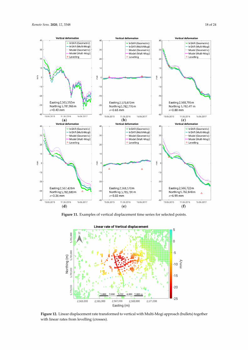
Figure 11 shows the vertical displacement for some time series for each of the approaches together with the model curves estimated and levelling. The model curves are a combination of three components: linear subsidence, pressure induced and seasonal displacement. The given value of σ is calculated for Multi-Mogi and is intended to convey a visual impression of the significance of the deviation that goes along with the value of σ. Figure 11d is an example where the non-modeled signal contains valuable information at locations, where the model does not fit perfectly to the time series.

Figure 8. Standard deviations of differences between InSAR results and levelling. Left-hand side fromgeometric orbit combination, right-hand side Multi-Mogi approach.

Figure 11 shows the vertical displacement for some time series for each of the approachestogether with the model curves estimated and levelling. The model curves are a combination of threecomponents: linear subsidence, pressure induced and seasonal displacement. The given value of σis calculated for Multi-Mogi and is intended to convey a visual impression of the significance of thedeviation that goes along with the value of σ. Figure 11d is an example where the non-modeled signalcontains valuable information at locations, where the model does not fit perfectly to the time series.

Remote Sens. 2020, 12, 3348 17 of 24

There are also cases where a larger deviation possibly is due to inaccuracies of levelling.Figure 11e shows a suspected case.


result and levelling at two regions, where the approximately north-south running levelling line leaves the subsidence bowl. Deviations for those using the Multi-Mogi approach are less severe. Two points with large deviation between the geometric approach and levelling stand out, while Multi-Mogi is not sensitive to estimation errors affecting single points by design and provides good results. This is

Figure 9. Histograms and scatter plots of differences between InSAR results and levelling. Left-hand side from geometric orbit combination, right-hand side Multi-Mogi approach.

Figure 10. Error of vertical displacement because of ignorance of north-south component.

There are also cases where a larger deviation possibly is due to inaccuracies of levelling. Figure 11e shows a suspected case.

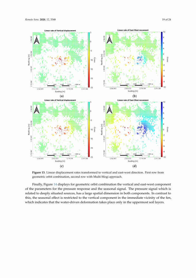
Figure 12 shows the linear vertical displacement rate estimated from the time series generated with the Multi-Mogi approach, where data have been interpolated to a raster. Linear rates for levelling points are displayed as crosses in the same color scale. Both data sets blend nicely, what demonstrates again the good agreement between results from Multi-Mogi and levelling measurements. It is clearly seen that the DS located at the fen carry relevant information about the convergence process of the caverns and thereby contribute to a spatially dense displacement field that could not have been obtained from PS alone. However, Multi-Mogi does not capture as well the horizontal displacement field as it does the vertical as indicates a comparison with the geometric approach. The first row of Figure 13 shows linear displacement rates in vertical and east-west

Figure 9. Histograms and scatter plots of differences between InSAR results and levelling. Left-hand sidefrom geometric orbit combination, right-hand side Multi-Mogi approach.


Figure 9. Histograms and scatter plots of differences between InSAR results and levelling. Left-hand side from geometric orbit combination, right-hand side Multi-Mogi approach.


There are also cases where a larger deviation possibly is due to inaccuracies of levelling. Figure 11e shows a suspected case.

Figure 12 shows the linear vertical displacement rate estimated from the time series generated with the Multi-Mogi approach, where data have been interpolated to a raster. Linear rates for levelling points are displayed as crosses in the same color scale. Both data sets blend nicely, what demonstrates again the good agreement between results from Multi-Mogi and levelling measurements. It is clearly seen that the DS located at the fen carry relevant information about the convergence process of the caverns and thereby contribute to a spatially dense displacement field that could not have been obtained from PS alone. However, Multi-Mogi does not capture as well the horizontal displacement field as it does the vertical as indicates a comparison with the geometric approach. The first row of Figure 13 shows linear displacement rates in vertical and east-west direction estimated from the time series generated with geometric orbit combination. The second row shows the corresponding results generated with the Multi-Mogi approach. The horizontal displacement extends far into the surroundings of the deposit and appears blurred in comparison with the result of the geometric combination.


Figure 12 shows the linear vertical displacement rate estimated from the time series generated withthe Multi-Mogi approach, where data have been interpolated to a raster. Linear rates for levelling pointsare displayed as crosses in the same color scale. Both data sets blend nicely, what demonstrates againthe good agreement between results from Multi-Mogi and levelling measurements. It is clearly seenthat the DS located at the fen carry relevant information about the convergence process of the cavernsand thereby contribute to a spatially dense displacement field that could not have been obtained fromPS alone. However, Multi-Mogi does not capture as well the horizontal displacement field as it doesthe vertical as indicates a comparison with the geometric approach. The first row of Figure 13 showslinear displacement rates in vertical and east-west direction estimated from the time series generatedwith geometric orbit combination. The second row shows the corresponding results generated with theMulti-Mogi approach. The horizontal displacement extends far into the surroundings of the depositand appears blurred in comparison with the result of the geometric combination.

Remote Sens. 2020, 12, 3348 18 of 24


(a)

(b)

(c)

(d)

(e)

(f)

Figure 11. Examples of vertical displacement time series for selected points.

Figure 12. Linear displacement rate transformed to vertical with Multi-Mogi approach (bullets) together with linear rates from levelling (crosses).



(a)

(b)

(c)

(d)

(e)

(f)


Figure 12. Linear displacement rate transformed to vertical with Multi-Mogi approach (bullets) together with linear rates from levelling (crosses).

Figure 12. Linear displacement rate transformed to vertical with Multi-Mogi approach (bullets) togetherwith linear rates from levelling (crosses).

Remote Sens. 2020, 12, 3348 19 of 24Remote Sens. 2020, 12, x FOR PEER REVIEW 19 of 24

(a)

(b)

(c)

(d)

Figure 13. Linear displacement rates transformed to vertical and east-west direction. First row from geometric orbit combination, second row with Multi-Mogi approach.

Finally, Figure 14 displays for geometric orbit combination the vertical and east-west component of the parameters for the pressure response and the seasonal signal. The pressure signal which is related to deeply situated sources, has a large spatial dimension in both components. In contrast to this, the seasonal effect is restricted to the vertical component in the immediate vicinity of the fen, which indicates that the water-driven deformation takes place only in the uppermost soil layers.

4. Discussion

The results presented in Section 3 demonstrate that multi-temporal InSAR techniques using Sentinel-1 data allow obtaining valuable information about complex surface displacement fields as that of the underground storage at Epe. The InSAR derived displacements are in reasonable agreement with levelling data for geometric orbit combination and in good agreement for the Multi-Mogi approach. They complement levelling with information from additional locations and deliver horizontal movements. In particular, a high temporal sampling is possible that is difficult to achieve with levelling. The successful analysis has been made possible by combining StaMPS with DS pre-processing and introducing a displacement model that improved unwrapping as well as orbit combination. DS allow to extract information also in areas, where no PS are available, in particular

Figure 13. Linear displacement rates transformed to vertical and east-west direction. First row fromgeometric orbit combination, second row with Multi-Mogi approach.

Finally, Figure 14 displays for geometric orbit combination the vertical and east-west componentof the parameters for the pressure response and the seasonal signal. The pressure signal which isrelated to deeply situated sources, has a large spatial dimension in both components. In contrast tothis, the seasonal effect is restricted to the vertical component in the immediate vicinity of the fen,which indicates that the water-driven deformation takes place only in the uppermost soil layers.

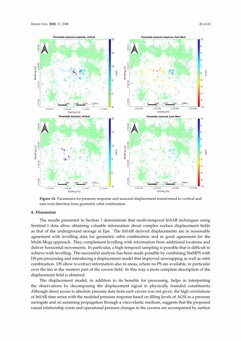
Remote Sens. 2020, 12, 3348 20 of 24


over the fen in the western part of the cavern field. In this way a more complete description of the displacement field is obtained.

Figure 14. Parameters for pressure response and seasonal displacement transformed to vertical and east-west direction from geometric orbit combination.

The displacement model, in addition to its benefits for processing, helps in interpreting the observations by decomposing the displacement signal in physically founded constituents. Although direct access to absolute pressure data from each cavern was not given, the high correlations of InSAR time series with the modeled pressure response based on filling levels of AGSI as a pressure surrogate and on assuming propagation through a visco-elastic medium, suggests that the proposed causal relationship exists and operational pressure changes in the caverns are accompanied by surface displacements of up to +/− 6 mm. The presented model driven approach facilitates a clear separation of the pressure related displacements from ground water induced surface movements.

The InSAR based results also exhibit some shortcomings. The results of the geometric approach for the vertical and east-west component of displacement suffer from ignorance of the north-south component but still are reasonable. The observed bias between InSAR and levelling can be explained partially by the required interpolation. On the other hand, the Multi-Mogi approach captures vertical displacement well. However, it does overestimate the magnitude of horizontal displacement. This shortcoming presumably can be accounted for by the following two arguments:

1. As already discussed above, the geophysical situation is simplistically modelled. In particular, the model assumes that the caverns each are in the center of a salt sphere while in reality the salt

Figure 14. Parameters for pressure response and seasonal displacement transformed to vertical andeast-west direction from geometric orbit combination.

4. Discussion

The results presented in Section 3 demonstrate that multi-temporal InSAR techniques usingSentinel-1 data allow obtaining valuable information about complex surface displacement fieldsas that of the underground storage at Epe. The InSAR derived displacements are in reasonableagreement with levelling data for geometric orbit combination and in good agreement for theMulti-Mogi approach. They complement levelling with information from additional locations anddeliver horizontal movements. In particular, a high temporal sampling is possible that is difficult toachieve with levelling. The successful analysis has been made possible by combining StaMPS withDS pre-processing and introducing a displacement model that improved unwrapping as well as orbitcombination. DS allow to extract information also in areas, where no PS are available, in particularover the fen in the western part of the cavern field. In this way a more complete description of thedisplacement field is obtained.

The displacement model, in addition to its benefits for processing, helps in interpretingthe observations by decomposing the displacement signal in physically founded constituents.Although direct access to absolute pressure data from each cavern was not given, the high correlationsof InSAR time series with the modeled pressure response based on filling levels of AGSI as a pressuresurrogate and on assuming propagation through a visco-elastic medium, suggests that the proposedcausal relationship exists and operational pressure changes in the caverns are accompanied by surface

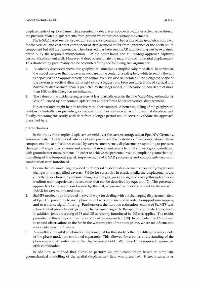
Remote Sens. 2020, 12, 3348 21 of 24

displacements of up to ± 6 mm. The presented model driven approach facilitates a clear separation ofthe pressure related displacements from ground water induced surface movements.

The InSAR based results also exhibit some shortcomings. The results of the geometric approachfor the vertical and east-west component of displacement suffer from ignorance of the north-southcomponent but still are reasonable. The observed bias between InSAR and levelling can be explainedpartially by the required interpolation. On the other hand, the Multi-Mogi approach capturesvertical displacement well. However, it does overestimate the magnitude of horizontal displacement.This shortcoming presumably can be accounted for by the following two arguments:

1. As already discussed above, the geophysical situation is simplistically modelled. In particular,the model assumes that the caverns each are in the center of a salt sphere while in reality the saltis deposited as an approximately horizontal layer. We also deliberated if the elongated shape ofthe caverns in vertical direction might cause a bigger ratio between magnitude of vertical andhorizontal displacement than is predicted by the Mogi model, but because of their depth of morethan 1000 m this likely has no influence.

2. The values of the incidence angles may at least partially explain that the Multi-Mogi estimation isless influenced by horizontal displacement and performs better for vertical displacement.

Future research might help to resolve these shortcomings. A better modeling of the geophysicalrealities potentially can provide good estimation of vertical as well as of horizontal displacement.Finally, repeating this study with data from a longer period would serve to validate the approachpresented here.

5. Conclusions

In this study the complex displacement field over the cavern storage site at Epe, NW-Germany,was investigated. The temporal behavior of each point could be modeled as linear combination of threecomponents: linear subsidence caused by cavern convergence, displacement responding to pressurechanges in the gas filled caverns and a seasonal movement over a fen that shows a good correlationwith groundwater measurements. In order to achieve the presented results, simplistic geomechanicalmodelling of the temporal signal, improvements of InSAR processing and component-wise orbitcombination were introduced.

1. Geomechanical modelling provided the temporal model for displacements responding to pressurechanges in the gas filled caverns. While for reservoirs in elastic media the displacements aredirectly proportional to pressure changes of the gas, pressure signals passing through a viscosmedium (salt) experience a retardation that can be described by equation (2). The presentedapproach is to the best of our knowledge the first, where such a model is derived for the use withInSAR for caverns situated in salt.

2. StaMPS needed to be improved in several ways for dealing with the challenging displacement fieldat Epe. The possibility to use a phase model was implemented in order to support unwrappingand to enhance signal filtering. Furthermore, the iterative estimation scheme of StaMPS wasrefined, what prevents leakage of the displacement signal to the spatially correlated noise term.In addition, joint processing of PS and DS as recently introduced in [20] was applied. The resultspresented in this study confirm the validity of the approach of [20]. In particular, the DS allowedto extend observations to the fen in the western part of the storage site, where no informationwas available with PS alone.

3. A novelty of the orbit combination implemented for this study is that the different componentsof the phase model are combined separately. This allowed for a better understanding of thephenomena that contribute to the displacement field. We named this approach geometricorbit combination.

In addition, a method that allows to perform an orbit combination based on simplisticgeomechanical modelling of the spatial displacement field was presented. It treats caverns as

Remote Sens. 2020, 12, 3348 22 of 24

Mogi sources, whose volume changes because of convergence lead to linear subsidence and whosepressure changes result in the pressure induced displacement. The model assumes for each of thesetwo components one unknown parameter that is estimated such that the projections to line of sightfor both orbits optimally approximate the orbit-wise estimations. We named this approach MultiMogi approach.

The vertical components of the estimated displacements were validated with data from 517 levellingpoints available over the storage site. The agreement of linear trends of vertical displacement fromgeometric orbit combination and levelling was reasonable (root mean square 3.41 mm/y). The agreementof linear trends of vertical displacement from the Multi Mogi approach and levelling was very good(root mean square 2.39 mm/y). Unfortunately, the Multi Mogi approach overestimated the east-westcomponent of displacement. This may be due to insufficient knowledge of physical parameters orimperfections of the model itself and deserves further investigation.

Author Contributions: Conceptualization, M.W.; methodology, M.E. and M.W.; software, M.E.; formal analysis,M.E.; preliminary analysis, V.S.; data curation, M.E. and V.S.; writing—original draft preparation, M.E.;writing—review and editing, M.W; visualization, M.E; project administration, M.W; funding acquisition, M.W.All authors have read and agreed to the published version of the manuscript.

Funding: The present study was financed by BMBF via the project SUBI. We thank BMBF for making ourwork possible.

Acknowledgments: We are grateful for the support and data we have received from our project partners fromSGW, in particular Stefan Meyer and Bernd Feldhaus, and from Uniper, in particular Bela Szöcs, Katrin Vosbeck,and Tobias Rudolph. We thank Andy Hooper for providing StaMPS as open source and ESA for the Sentinel-1data and SNAP (Sentinel Application Platform).

Conflicts of Interest: The authors declare no conflict of interest. The funders had no role in the design of thestudy; in the collection, analyses, or interpretation of data; in the writing of the manuscript, or in the decision topublish the results.

References

1. Vasco, D.W.; Ferretti, A.; Novali, F. Estimating permeability from quasi-static deformation:Temporal variations and arrival-time inversion. Geophysics 2008, 73, O37–O52. [CrossRef]

2. Vasco, D.W.; Ferretti, A.; Novali, F. Reservoir monitoring and characterization using satellite geodetic data:Interferometric synthetic aperture radar observations from the Krechba field, Algeria. Geophysics 2008, 73,WA113–WA122. [CrossRef]

3. Vasco, D.W.; Rucci, A.; Ferretti, A.; Novali, F.; Bissell, R.C.; Ringrose, P.S.; Mathieson, A.S.; Wright, I.W.Satellite-based measurements of surface deformation reveal fluid flow associated with the geological storageof carbon dioxide. Geophys. Res. Lett. 2010, 37, 1–5. [CrossRef]

4. Tamburini, A.; Bianchi, M.; Giannico, C.; Novali, F. Retrieving surface deformation by PSInSARTM technology:A powerful tool in reservoir monitoring. Int. J. Greenh. Gas Control 2010, 4, 928–937. [CrossRef]

5. Rucci, A.; Vasco, D.W.; Novali, F. Fluid pressure arrival time tomography: Estimation and assessment in thepresence of inequality constraints, with an application to production at the Krechba field, Algeria. Geophysics2010, 75, 39–55. [CrossRef]

6. Rocca, F.; Rucci, A.; Ferretti, A.; Bohane, A. Advanced InSAR interferometry for reservoir monitoring.First Break 2013, 31, 77–85.

7. Rucci, A.; Vasco, D.W.; Novali, F. Monitoring the geologic storage of carbon dioxide using multicomponentSAR interferometry. Geophys. J. Int. 2013, 193, 197–208. [CrossRef]

8. Teatini, P.; Castelletto, N.; Ferronato, M.; Gambolati, G.; Janna, C.; Cairo, E.; Marzorati, D.; Colombo, D.;Ferretti, A.; Bagliani, A.; et al. Geomechanical response to seasonal gas storage in depleted reservoirs: A casestudy in the Po River basin, Italy. J. Geophys. Res. Space Phys. 2011, 116. [CrossRef]

9. Fokker, P.A.; Visser, K.; Peters, E.; Kunakbayeva, G.; Muntendam-Bos, A. Inversion of surface subsidencedata to quantify reservoir compartmentalization: A field study. J. Pet. Sci. Eng. 2012, 10–21. [CrossRef]

10. Comola, F.; Janna, C.; Lovison, A.; Minini, M.; Tamburini, A.; Teatini, P. Efficient global optimization ofreservoir geomechanical parameters based on synthetic aperture radar-derived ground displacements.Geophysics 2016, 81, M23–M33. [CrossRef]

http://dx.doi.org/10.1190/1.2978164

http://dx.doi.org/10.1190/1.2981184

http://dx.doi.org/10.1029/2009GL041544

http://dx.doi.org/10.1016/j.ijggc.2009.12.009

http://dx.doi.org/10.1190/1.3493504

http://dx.doi.org/10.1093/gji/ggs112

http://dx.doi.org/10.1029/2010JF001793

http://dx.doi.org/10.1016/j.petrol.2012.06.032

http://dx.doi.org/10.1190/geo2015-0402.1

Remote Sens. 2020, 12, 3348 23 of 24

11. Velasco, V.; Sanchez, C.; Papoutsis, I.; Antoniadi, S.; Kontoes, C.; Aifantopoulou, D.; Paralykidis, S. Grounddeformation mapping and monitoring of salt mines using InSAR technology. In Proceedings of the SolutionMining Research Institute Fall 2017 Technical Conference, Münster, Germany, 25–26 September 2017.

12. Burnol, A.; Aochi, H.; Raucoules, D.; Veloso, F.M.L.; Koudogbo, F.N.; Fumagalli, A.; Chiquet, P.; Maisons, C.Wavelet-based analysis of ground deformation coupling satellite acquisitions (Sentinel-1, SMOS) and datafrom shallow and deep wells in Southwestern France. Sci. Rep. 2019, 9, 1–12. [CrossRef]

13. Ferretti, A.; Tamburini, A.; Novali, F.; Fumagalli, A.; Falorni, G.; Rucci, A. Impact of high resolution radarimagery on reservoir monitoring. Energy Procedia 2011, 4, 3465–3471. [CrossRef]

14. Kuehn, F.; Hoth, P.; Stark, M.; Burren, R.; Hole, J. Experience with satellite radar for gas storage monitoring.Erdöl Erdgas Kohle 2009, 125, 452–460.

15. Jha, B.; Bottazzi, F.; Wojcik, R.; Coccia, M.; Bechor, N.; McLaughlin, D.; Herring, T.; Hager, B.H.; Mantica, S.;Juanes, R. Reservoir characterization in an underground gas storage field using joint inversion of flow andgeodetic data. Int. J. Numer. Anal. Methods Géoméch. 2015, 39, 1619–1638. [CrossRef]

16. Morgan, J.; Snider-Lord, A.C.; Ambs, D.C. InSAR for monitoring cavern integrity: 2D surface movement overBryan Mound. In Proceedings of the Solution Mining Research Institute Spring 2018 Technical Conference,Salt Lake City, UT, USA, 18 June 2018.

17. Meyers, M.A.; Chawla, K.K. Mechanical Behavior of Materials, 2nd ed.; Cambridge University Press: New York,NY, USA, 2009; pp. 1–856.

18. Ferretti, A.; Fumagalli, A.; Novali, F.; Prati, C.; Rocca, F.; Rucci, A. A new algorithm for processinginterferometric data-stacks: SqueeSAR. IEEE Trans. Geosci. Remote Sens. 2011, 49, 3460–3470. [CrossRef]

19. Even, M.; Schulz, K. InSAR deformation analysis with distributed scatterers: A review complemented bynew advances. Remote Sens. 2018, 10, 744. [CrossRef]

20. Even, M. Adapting stamps for jointly processing distributed scatterers and persistent scatterers.In Proceedings of the IGARSS 2019–2019 IEEE International Geoscience and Remote Sensing Symposium,Yokohama, Japan, 28 July–2 August 2019; pp. 2046–2049. [CrossRef]

21. Hooper, A.; Segall, P.; Zebker, H. Persistent scatterer interferometric synthetic aperture radar for crustaldeformation analysis, with application to Volcán Alcedo, Galápagos. J. Geophys. Res. Space Phys. 2007, 112,1–21. [CrossRef]

22. StaMPS Homepage. Available online: https://homepages.see.leeds.ac.uk/~earahoo/stamps/ (accessed on 12September 2013).

23. Gray, L. Using multiple RADARSAT InSAR pairs to estimate a full three-dimensional solution for glacial icemovement. Geophys. Res. Lett. 2011, 38, 1–6. [CrossRef]

24. Hu, J.; Li, Z.; Ding, X.; Zhu, J.; Zhang, L.; Sun, Q. Resolving three-dimensional surface displacements fromInSAR measurements: A review. Earth Sci. Rev. 2014, 133, 1–17. [CrossRef]

25. Joughin, I.; Kwok, R.; Fahnestock, M. Interferometric estimation of three-dimensional ice-flow usingascending and descending passes. IEEE Trans. Geosci. Remote Sens. 1998, 36, 25–37. [CrossRef]

26. Mohr, J.J.; Reeh, N.; Madsen, S.N. Three-dimensional glacial flow and surface elevation measured with radarinterferometry. Nature 1998, 391, 273–276. [CrossRef]

27. Cascini, L.; Fornaro, G.; Peduto, D. Advanced low and full-resolution DInSAR map generation forslow-moving landslide analysis at different scales. Eng. Geol. 2010, 112, 29–42. [CrossRef]

28. Bos, A.G.; Usai, S.; Spakman, W. A joint analysis of GPS motions and InSAR to infer the coseismic surfacedeformation of the Izmit, Turkey earthquake. Geophys. J. Int. 2004, 158, 849–863. [CrossRef]

29. Fuhrmann, T.; Cuenca, M.C.; Knöpfler, A.; Van Leijen, F.; Mayer, M.; Westerhaus, M.; Hanssen, R.; Heck, B.Estimation of small surface displacements in the Upper Rhine Graben area from a combined analysis ofPS-InSAR, levelling and GNSS data. Geophys. J. Int. 2015, 203, 614–631. [CrossRef]

30. Michel, R.; Avouac, J.-P.; Taboury, J.; Michel, R. Measuring ground displacements from SAR amplitudeimages: Application to the Landers Earthquake. Geophys. Res. Lett. 1999, 26, 875–878. [CrossRef]

31. Michel, R.; Avouac, J.-P.; Taboury, J. Measuring near field coseismic displacements from SAR images:Application to the Landers Earthquake. Geophys. Res. Lett. 1999, 26, 3017–3020. [CrossRef]

32. Bechor, N.B.D.; Zebker, H.A. Measuring two-dimensional movements using a single InSAR pair.Geophys. Res. Lett. 2006, 33, 1–5. [CrossRef]

http://dx.doi.org/10.1038/s41598-019-45302-z

http://dx.doi.org/10.1016/j.egypro.2011.02.272

http://dx.doi.org/10.1002/nag.2427

http://dx.doi.org/10.1109/TGRS.2011.2124465

http://dx.doi.org/10.3390/rs10050744

http://dx.doi.org/10.1109/igarss.2019.8897808

http://dx.doi.org/10.1029/2006JB004763

https://homepages.see.leeds.ac.uk/~earahoo/stamps/

http://dx.doi.org/10.1029/2010GL046484

http://dx.doi.org/10.1016/j.earscirev.2014.02.005

http://dx.doi.org/10.1109/36.655315

http://dx.doi.org/10.1038/34635

http://dx.doi.org/10.1016/j.enggeo.2010.01.003

http://dx.doi.org/10.1111/j.1365-246X.2004.02359.x

http://dx.doi.org/10.1093/gji/ggv328

http://dx.doi.org/10.1029/1999GL900138

http://dx.doi.org/10.1029/1999GL900524

http://dx.doi.org/10.1029/2006GL026883

Remote Sens. 2020, 12, 3348 24 of 24

33. Samiei-Esfahany, S.; Hanssen, R.; van Thienen-Visser, K.; Muntendam-Bos, A. On the effect of horizontaldeformation on InSAR subsidence estimates. In Proceedings of the Fringe Workshop, ESRIN, Frascati, Italy,30 November–4 December 2009.

34. Wright, T.J.; Parsons, B.E.; Lu, Z. Toward mapping surface deformation in three dimensions using InSAR.Geophys. Res. Lett. 2004, 31, 1–5. [CrossRef]

35. Manzo, M.; Ricciardi, G.; Casu, F.; Ventura, G.; Zeni, G.; Borgström, S.; Berardino, P.; Del Gaudio, C.;Lanari, R. Surface deformation analysis in the Ischia Island (Italy) based on spaceborne radar interferometry.J. Volcanol. Geotherm. Res. 2006, 151, 399–416. [CrossRef]

36. Fuhrmann, T.; Garthwaite, M.C. Resolving three-dimensional surface motion with InSAR: Constraints frommulti-geometry data fusion. Remote Sens. 2019, 11, 241. [CrossRef]

37. Mogi, K. Relations between the eruptions of various volcanoes and the deformations of the ground surfacesaround them. Earthq. Res. Inst. 1958, 36, 99–134.

38. Aggregated Gas Storage Inventory (AGSI). Available online: https://agsi.gie.eu/#/ (accessed on 5 December2019).

39. Liu, W.; Völkner, E.; Minkley, W.; Popp, T. F+E Endlagerung: Zusammenstellung der Materialparameter fürTHM-Modellberechnungen, Ergebnisse aus dem Vorhaben KOSINA; Bundesanstalt für Geowissenschaften undRohstoffe: Hannover, Germany, 2017.

40. Shamshiri, R.; Nahavandchi, H.; Motagh, M.; Hooper, A. Efficient ground surface displacement monitoringusing sentinel-1 data: Integrating Distributed Scatterers (DS) identified using two-sample t-test withPersistent Scatterers (PS). Remote Sens. 2018, 10, 794. [CrossRef]

41. Pepe, A.; Yang, Y.; Manzo, M.; Lanari, R. Improved EMCF-SBAS processing chain based on advancedtechniques for the noise-filtering and selection of small baseline multi-look DInSAR Interferograms.IEEE Trans. Geosci. Remote Sens. 2015, 53, 4394–4417. [CrossRef]

42. Wang, Y.; Zhu, X.X. Robust estimators for multipass SAR interferometry. IEEE Trans. Geosci. Remote Sens.2015, 54, 968–980. [CrossRef]

43. Samiei-Esfahany, S.; Martins, J.E.; Van Leijen, F.; Hanssen, R.F. Phase estimation for distributed scatterers inInSAR stacks using integer least squares estimation. IEEE Trans. Geosci. Remote Sens. 2016, 54, 5671–5687.[CrossRef]

44. Lin, K.-F.; Perissin, D. Identification of statistically homogeneous pixels based on one-sample test. Remote Sens.2017, 9, 37. [CrossRef]

45. Verde, S.; Reale, D.; Pauciullo, A.; Fornaro, G. Improved small baseline processing by means of CAESAReigen-interferograms decomposition. ISPRS J. Photogramm. Remote Sens. 2018, 139, 1–13. [CrossRef]

46. Ansari, H.; De Zan, F.; Bamler, R. Efficient phase estimation for interferogram stacks. IEEE Trans. Geosci.Remote Sens. 2018, 56, 4109–4125. [CrossRef]

47. Ferretti, A.; Fumagalli, A.; Novali, F.; De Zan, F.; Rucci, A.; Tebaldini, S. Process for Filtering InterferogramsObtained from SAR Images Acquired on the Same Area. CA Patent Application 2,767,144, 13 January 2011.

48. Guarnieri, A.M.; Tebaldini, S. On the exploitation of target statistics for SAR interferometry applications.IEEE Trans. Geosci. Remote Sens. 2008, 46, 3436–3443. [CrossRef]

49. Wackernagel, H. Multivariate Geostatistics, 3rd ed.; Springer: Berlin/Heidelberg, Germany, 2003; pp. 1–387.50. Samsonov, S.V.; D’Oreye, N. Multidimensional Small Baseline Subset (MSBAS) for two-dimensional

deformation analysis: Case study Mexico City. Can. J. Remote Sens. 2017, 43, 318–329. [CrossRef]51. Morishita, Y.; Hanssen, R.F. Temporal decorrelation in L-, C-, and X-band satellite radar interferometry for

pasture on drained peat soils. IEEE Trans. Geosci. Remote Sens. 2014, 53, 1096–1104. [CrossRef]52. Morishita, Y.; Hanssen, R.F. Deformation parameter estimation in low coherence areas using a multisatellite

InSAR approach. IEEE Trans. Geosci. Remote Sens. 2015, 53, 4275–4283. [CrossRef]

Publisher’s Note: MDPI stays neutral with regard to jurisdictional claims in published maps and institutionalaffiliations.

© 2020 by the authors. Licensee MDPI, Basel, Switzerland. This article is an open accessarticle distributed under the terms and conditions of the Creative Commons Attribution(CC BY) license (http://creativecommons.org/licenses/by/4.0/).

http://dx.doi.org/10.1029/2003GL018827

http://dx.doi.org/10.1016/j.jvolgeores.2005.09.010

http://dx.doi.org/10.3390/rs11030241

https://agsi.gie.eu/#/

http://dx.doi.org/10.3390/rs10050794




http://dx.doi.org/10.3390/rs9010037

http://dx.doi.org/10.1016/j.isprsjprs.2018.02.019



http://dx.doi.org/10.1080/07038992.2017.1344926



http://creativecommons.org/

http://creativecommons.org/licenses/by/4.0/.

complex surface displacements above the storage cavern

Documents