This article appeared in a journal published by Elsevier. The attachedcopy is furnished to the author for internal non-commercial researchand education use, including for instruction at the authors institution

and sharing with colleagues.

Other uses, including reproduction and distribution, or selling orlicensing copies, or posting to personal, institutional or third party

websites are prohibited.

In most cases authors are permitted to post their version of thearticle (e.g. in Word or Tex form) to their personal website orinstitutional repository. Authors requiring further information

regarding Elsevier’s archiving and manuscript policies areencouraged to visit:

http://www.elsevier.com/copyright

Author's personal copy

Engineering Structures 30 (2008) 1262–1271www.elsevier.com/locate/engstruct

Global and local seismic drift estimates for RC frames

JoAnn Browninga,∗, Branden Wardenb, Adolfo Matamorosa, Andres Lepagec

a University of Kansas, 2150 Learned Hall, Lawrence, KS 66045, USAb E.I.T., Mettemeyer Engineering, LLC., 2101 W. Chesterfield Blvd., Suite B105, Springfield, MO 65807, USA

c The Pennsylvania State University, 104 Engineering Unit A, University Park, PA 16802, USA

Received 6 December 2006; received in revised form 27 June 2007; accepted 2 July 2007Available online 4 September 2007

Abstract

The relationship between reinforced concrete building displacement responses to seismic loading calculated using multi-degree-of-freedom(MDOF) nonlinear models and equivalent single-degree-of-freedom (SDOF) and MDOF linear models is examined. Displacement response ischaracterized by the peak roof drift (global deformation), maximum story distortion (local deformation) and the distortion location. A simplerelationship between nonlinear peak roof drift, linear response spectrum, and effective building period is determined from parametric analysis ofa set of frames subjected to a suite of ground motions. The relationship is expressed in terms of initial period using uncracked sections, a periodfactor, and a linear displacement response spectrum of particular equivalent damping. The best relationship was found to be in terms of the initialperiod factored by 2.0 and 2.3 for moderate and high seismicity ground motion, respectively, and using a 10%-damped linear response spectrum.The optimal period factor remained nearly constant for linear spectra with damping between 6% and 12%. A relationship between maximum storydistortion for linear MDOF systems and nonlinear MDOF systems was sought in terms of maximum value and location. The ratios of maximumstory distortions for nonlinear and linear analyses were found to vary significantly, as did the ratios between locations of these values. On average,the maximum story drift ratio from nonlinear analysis was 1.5 times the value calculated from linear analysis.c© 2007 Elsevier Ltd. All rights reserved.

Keywords: Concrete frames; Simplified analysis; Drift

1. Introduction

Simple estimates of the nonlinear response of reinforcedconcrete building structures will always be needed as longas engineers use experience and judgment to assess theadequacy of structural designs in seismic regions. For youngengineers, whose sum total of experience may be modest,methods to quickly estimate response parameters and comparewith detailed analysis are essential. A greater number ofengineers may benefit in regions of moderate seismicity wheretime-consuming detailed analyses are often not economicallyfeasible.

Several methods for estimating nonlinear response quantitiesfor reinforced concrete buildings have evolved using linear

∗ Corresponding address: University of Kansas, CEAE Department, 2150Learned Hall, Lawrence, KS 66045, USA. Tel.: +1 785 864 3723; fax: +1 785864 5631.

E-mail address: jpbrown@ku.edu (J. Browning).

analysis with an effective stiffness (or period) to account for the“softening” of the structure during response to strong groundmotion. Early experimental and analytical work showed thattwo basic phenomena influenced the peak response quantitiesof reinforced concrete structures: a reduction in stiffness and anincrease in energy-dissipation [1]. These ideas were quantifiedin the substitute-structure method as a design tool that enabledengineers to estimate the minimum strengths required for eachof the structural members, so as not to exceed anticipateddisplacements [2]. The substitute-structure method stems fromthe idea that an inelastic response can be represented by a linearresponse “substitute” using an effective stiffness and effectivedamping definitions based on the amount of damage expectedin the structure.

Shimazaki and Sozen [3] found that the maximum nonlineardisplacement is essentially unaffected by the base shearstrength for systems with a fundamental period greater thanthe characteristic period Tg , the period defined on a responsespectrum at which the nearly constant acceleration response

0141-0296/$ - see front matter c© 2007 Elsevier Ltd. All rights reserved.doi:10.1016/j.engstruct.2007.07.003

Author's personal copy

J. Browning et al. / Engineering Structures 30 (2008) 1262–1271 1263

region ends. A simple relationship between the maximumdisplacement response and the period of the linear systemwas established using an idealized displacement responsespectrum with 2% damping and an SDOF system with aneffective period Teff equal to the initial period (calculatedwith uncracked section properties) multiplied by

√2. The

nonlinear displacement response was then calculated as thelinear response of a system with period Teff. This methodprovided a reasonable upper bound for displacement responseof structures having periods that are longer than Tg . Lepage [4]completed the method by showing that for systems havingperiods less than the characteristic period of the earthquake andminimal base shear strength, nonlinear displacement responsecould be estimated using a modified smooth displacementresponse spectrum. This modified spectrum was based onextending the nearly constant velocity region through zeroperiod. Thus, for periods less than Tg , nonlinear displacementsexceed linear displacements.

Other efforts to characterize nonlinear drift using SDOFmodels offer various levels of complexity to estimate maximumresponse. One such variation is to estimate an optimumeffective period and damping as functions of ductilityratio [5–7]. Another approach is to estimate the maximumresponse of the inelastic SDOF system as a product of themaximum deformation of a linear elastic system (with thesame initial stiffness and damping as that of the inelasticsystem) and a displacement modification factor [8,9]. Moredetailed estimates of effective period have been proposed [10,11] by implementing the secant stiffness similar to thesubstitute-structure method, where the period of vibration ofthe equivalent linear system is calculated at the maximumanticipated deformation using the equivalent stiffness, the post-yield stiffness to initial stiffness ratio, and the ductility ratio.The equivalent viscous damping is also related to the ductilityratio.

The frequency of work developing simple linear SDOFmodels to estimate nonlinear response reflects the demand bythe profession to efficiently determine if a structural layoutis sufficient for a given earthquake risk. Yet, the describedstudies have focused on comparing nonlinear SDOF responsewith linear SDOF response quantities, so that the nonlinearMDOF response aspects (including maximum story distortion)are not addressed. This study identifies the best linear SDOFmodel to describe the nonlinear MDOF response of RC framesproportioned for regions of high and moderate seismicity. Inaddition, the maximum story distortion and its location innonlinear MDOF analysis for a region of high seismic risk isapproximated based on the results of linear MDOF analysis.

2. Research significance

Simplified methods are needed to estimate nonlinearresponse of building structures. Whereas the previous studieshave investigated the correlation between linear and nonlinearresponse of SDOF systems, the current study directly relateslinear SDOF response to nonlinear MDOF response. Theconclusions from this study allow an engineer to directly

estimate peak roof drift, maximum nonlinear story distortion,and the location of maximum building distortion based on alinear analysis.

3. Parametric analysis

A simple relationship between nonlinear peak roof drift,linear response spectra, and effective building period isdetermined from parametric analysis using 105 reinforcedconcrete frames and a suite of 10 ground motions. The materialproperties for the concrete included a compressive strengthf ′c equal to 28 MPa, an average modulus of elasticity of

28 GPa, and a shear modulus of 11 GPa. The yield stress ofthe reinforcing steel was assumed to be 414 MPa. Each framehad three bays and ranged in height from 5 to 17 stories, in2-story increments. Bay widths were either 6.1 or 9.1 m. Thefirst floor story heights were 3.0, 3.7, and 4.9 m. For the caseshaving 4.9-m first stories, the typical story height was 3.0 m,all other cases had typical story heights that were uniform overthe height of the building. The girders were proportioned usingdepths of one-twelfth the total span length. Additional caseswith girder depth of one-tenth the span length were consideredonly for regions of high seismicity and 6.1-m bays. Thus, a totalof 63 building frames were considered as having high seismicrisk, and 42 as moderate seismic risk.

The frames were proportioned to encompass a large rangeof stiffness configurations and initial periods for two regions ofseismicity: high and moderate seismic risk. The representativespectra were based on the simplified spectral displacementcurve Sd used by Matamoros et al. [12]:

Sd =SD1

(2π)2 Teff (1)

with SD1 the one second spectral acceleration as defined inIBC 2006 [13], and Teff the effective period as defined byShimazaki and Sozen [3]. The value of SD1 was set equal to1.0g for a region of high seismicity and equal to 0.5g for aregion of moderate seismicity, where g is the acceleration ofgravity. Although the selected SD1 = 1.0g could be foundat many sites on the west coast of the United States, it is ofinterest to note that SD1 = 0.5g is representative of a stiffsoil site in Memphis, Tennessee. Using these spectral demands,frames were proportioned to limit the estimated maximum roofdrift to approximately 1.5% of the total building height. Driftwas calculated using the linear response spectrum defined byEq. (1) and applying the equal displacement rule (Cd = R asdefined in ASCE 7 [14]). Dimensions for square column cross-sections are listed in Table 1, and were found to be reasonablewhen compared with the existing structures in similar regionsof seismicity. For the region of moderate seismic risk, gravityload demands were the controlling proportioning criterion.The gravity load (7.7 kN/m2) was assumed to act over atributary width equal to the bay length. A change in columncross-sections was designed near mid-height of the buildingfor structures greater than 7 stories in height. Reinforcementratios in the proportioned members averaged 0.75% in thegirders, and the columns had 2% and 1% reinforcement ratios

Author's personal copy

1264 J. Browning et al. / Engineering Structures 30 (2008) 1262–1271

Table 1Column proportions

No. of stories Bay width (m) Story height (m) High seismicity Moderate seismicityGirder depth = L/12 Girder depth = L/10 Girder depth = L/12Column Column ColumnBase (cm) Top (cm) Base (cm) Top (cm) Base (cm) Top (cm)

5 6.1 3.0 71 71 51 51 41 416.1 3.7 71 71 56 56 41 416.1 3.0a 76 76 61 61 41 41

9.1 3.0 66 66 56 569.1 3.7 71 71 56 569.1 3.0a 76 76 56 56

7 6.1 3.0 71 71 51 51 41 416.1 3.7 76 76 56 56 41 416.1 3.0a 76 76 61 61 41 41

9.1 3.0 66 66 61 619.1 3.7 71 71 61 619.1 3.0a 76 76 61 61

9 6.1 3.0 76 71 51 51 46 416.1 3.7 81 71 56 51 46 416.1 3.0a 81 71 61 46 46 41

9.1 3.0 76 56 71 569.1 3.7 76 61 71 569.1 3.0a 81 61 71 56

11 6.1 3.0 81 71 51 51 51 416.1 3.7 81 76 56 51 51 416.1 3.0a 81 76 61 46 51 41

9.1 3.0 76 56 76 619.1 3.7 81 61 76 619.1 3.0a 81 61 76 61

13 6.1 3.0 81 76 56 46 56 416.1 3.7 86 76 56 56 56 416.1 3.0a 86 76 66 46 56 41

9.1 3.0 81 61 86 619.1 3.7 81 61 86 619.1 3.0a 81 61 86 61

15 6.1 3.0 86 76 56 46 61 466.1 3.7 86 81 66 46 61 466.1 3.0a 86 81 61 46 61 46

9.1 3.0 86 61 91 669.1 3.7 86 61 91 669.1 3.0a 86 61 91 66

17 6.1 3.0 86 81 61 46 66 466.1 3.7 86 86 66 46 66 466.1 3.0a 86 86 61 46 66 46

9.1 3.0 91 66 97 719.1 3.7 91 66 97 719.1 3.0a 91 66 97 71

a Tall first story (4.9 m) with 3.0-m stories above.

when proportioned for regions of high and moderate seismicity,respectively.

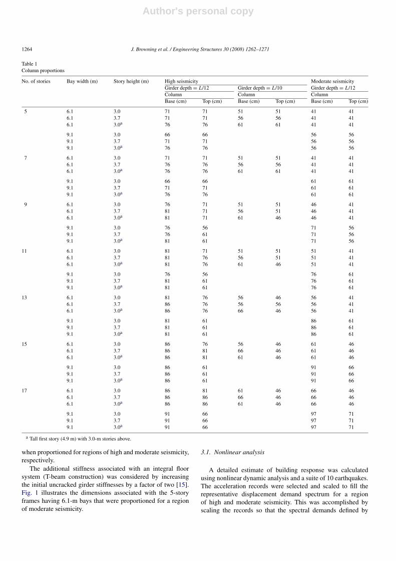
The additional stiffness associated with an integral floorsystem (T-beam construction) was considered by increasingthe initial uncracked girder stiffnesses by a factor of two [15].Fig. 1 illustrates the dimensions associated with the 5-storyframes having 6.1-m bays that were proportioned for a regionof moderate seismicity.

3.1. Nonlinear analysis

A detailed estimate of building response was calculatedusing nonlinear dynamic analysis and a suite of 10 earthquakes.The acceleration records were selected and scaled to fill therepresentative displacement demand spectrum for a regionof high and moderate seismicity. This was accomplished byscaling the records so that the spectral demands defined by

Author's personal copy

J. Browning et al. / Engineering Structures 30 (2008) 1262–1271 1265

Table 2Properties of ground motions

Earthquake Station Source Recordduration (s)

Characteristicperiod Tg (s)

Scaled peakgroundacceleration(Moderate) (g)

Scaled peakgroundacceleration(High) (g)

San Fernando02-09-1971

Castaic, (CAS)Old Ridge Route, CA

CALTECH [22] 30 0.35 0.39 0.78

Northridge01-17-1994

Tarzana, (TAR)Cedar Hill Nursery, CA

CSMIP [23] 30 0.44 0.31 0.62

Chile03-03-1985

Llolleo, (LLO)D.I.C., Chile

Saragoni et al. [24] 75 0.50 0.28 0.55

Imperial Valley05-18-1940

El Centro, (ELC)Irrigation Distric, CA

CALTECH [25] 45 0.55 0.25 0.50

Hyogo-Ken-Nanbu01-17-1995

Kobe, (KOB)KMMO, Japan

JMA [26] 30a 0.70 0.20 0.39

Kern County07-21-1952

Taft, (TAF)Lincoln School Tunnel, CA

CALTECH [25] 45 0.72 0.19 0.38

Western Washington04-13-1949

Seattle, (SEA)Army Base, WA

CALTECH [27] 65 0.89 0.15 0.31

Miyagi-Ken-Oki04-13-1949

Sendai, (SEN)Tohoku University, Japan

Mori and Crouse [28] 40 0.95 0.14 0.29

Kern County07-21-1952

Santa Barbara, (SAB)Courthouse, CA

CALTECH [25] 60 1.03 0.13 0.27

Tokachi-Oki05-16-1968

Hachinohe, (HAC)Harbor, Japan

Mori and Crouse [28] 35 1.14 0.12 0.24

a Notes: Cut from original record at 25 s.

Fig. 1. 5-story frames with 6.1-m bays in region of moderate seismicity.

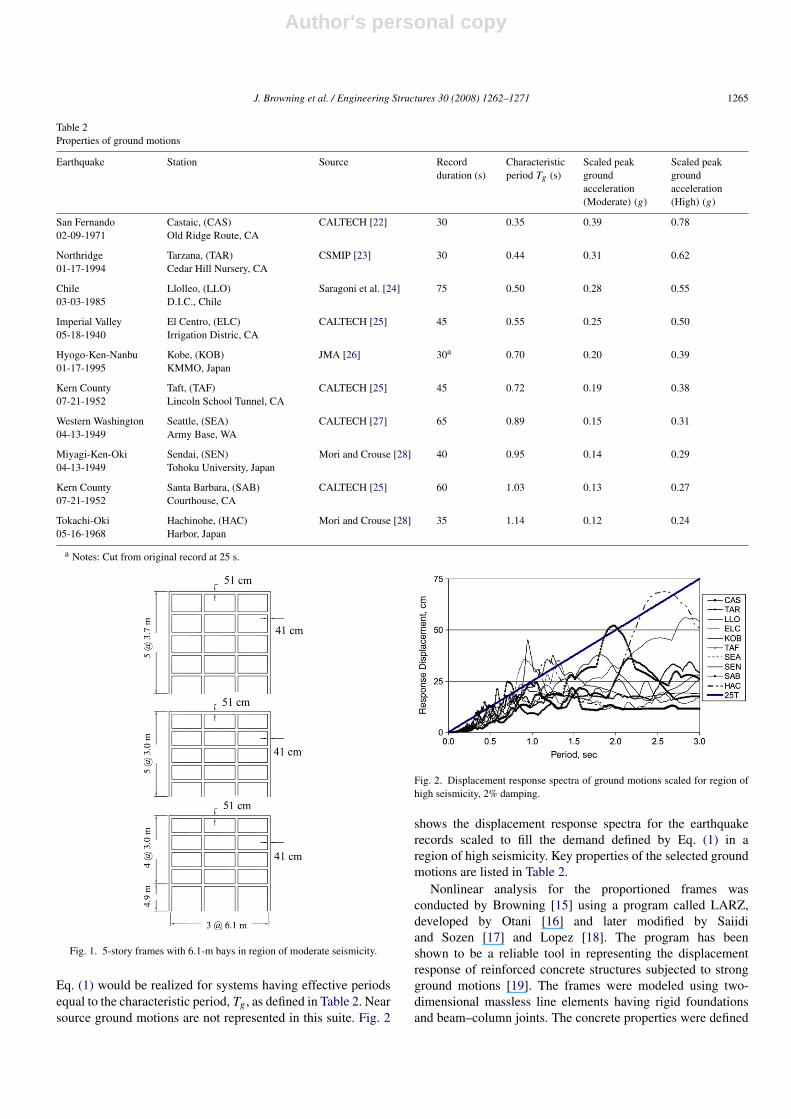
Eq. (1) would be realized for systems having effective periodsequal to the characteristic period, Tg , as defined in Table 2. Nearsource ground motions are not represented in this suite. Fig. 2

Fig. 2. Displacement response spectra of ground motions scaled for region ofhigh seismicity, 2% damping.

shows the displacement response spectra for the earthquakerecords scaled to fill the demand defined by Eq. (1) in aregion of high seismicity. Key properties of the selected groundmotions are listed in Table 2.

Nonlinear analysis for the proportioned frames wasconducted by Browning [15] using a program called LARZ,developed by Otani [16] and later modified by Saiidiand Sozen [17] and Lopez [18]. The program has beenshown to be a reliable tool in representing the displacementresponse of reinforced concrete structures subjected to strongground motions [19]. The frames were modeled using two-dimensional massless line elements having rigid foundationsand beam–column joints. The concrete properties were defined

Author's personal copy

1266 J. Browning et al. / Engineering Structures 30 (2008) 1262–1271

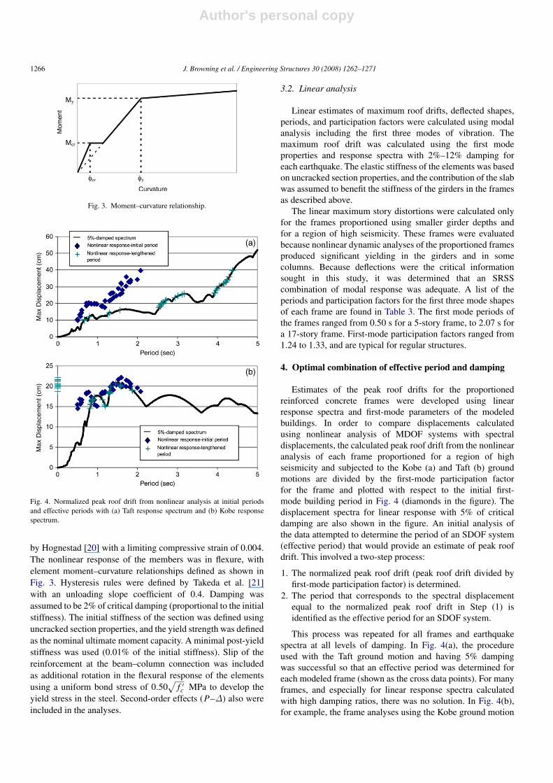
Fig. 3. Moment–curvature relationship.

Fig. 4. Normalized peak roof drift from nonlinear analysis at initial periodsand effective periods with (a) Taft response spectrum and (b) Kobe responsespectrum.

by Hognestad [20] with a limiting compressive strain of 0.004.The nonlinear response of the members was in flexure, withelement moment–curvature relationships defined as shown inFig. 3. Hysteresis rules were defined by Takeda et al. [21]with an unloading slope coefficient of 0.4. Damping wasassumed to be 2% of critical damping (proportional to the initialstiffness). The initial stiffness of the section was defined usinguncracked section properties, and the yield strength was definedas the nominal ultimate moment capacity. A minimal post-yieldstiffness was used (0.01% of the initial stiffness). Slip of thereinforcement at the beam–column connection was includedas additional rotation in the flexural response of the elementsusing a uniform bond stress of 0.50

√f ′c MPa to develop the

yield stress in the steel. Second-order effects (P–∆) also wereincluded in the analyses.

3.2. Linear analysis

Linear estimates of maximum roof drifts, deflected shapes,periods, and participation factors were calculated using modalanalysis including the first three modes of vibration. Themaximum roof drift was calculated using the first modeproperties and response spectra with 2%–12% damping foreach earthquake. The elastic stiffness of the elements was basedon uncracked section properties, and the contribution of the slabwas assumed to benefit the stiffness of the girders in the framesas described above.

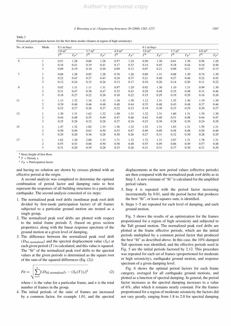
The linear maximum story distortions were calculated onlyfor the frames proportioned using smaller girder depths andfor a region of high seismicity. These frames were evaluatedbecause nonlinear dynamic analyses of the proportioned framesproduced significant yielding in the girders and in somecolumns. Because deflections were the critical informationsought in this study, it was determined that an SRSScombination of modal response was adequate. A list of theperiods and participation factors for the first three mode shapesof each frame are found in Table 3. The first mode periods ofthe frames ranged from 0.50 s for a 5-story frame, to 2.07 s fora 17-story frame. First-mode participation factors ranged from1.24 to 1.33, and are typical for regular structures.

4. Optimal combination of effective period and damping

Estimates of the peak roof drifts for the proportionedreinforced concrete frames were developed using linearresponse spectra and first-mode parameters of the modeledbuildings. In order to compare displacements calculatedusing nonlinear analysis of MDOF systems with spectraldisplacements, the calculated peak roof drift from the nonlinearanalysis of each frame proportioned for a region of highseismicity and subjected to the Kobe (a) and Taft (b) groundmotions are divided by the first-mode participation factorfor the frame and plotted with respect to the initial first-mode building period in Fig. 4 (diamonds in the figure). Thedisplacement spectra for linear response with 5% of criticaldamping are also shown in the figure. An initial analysis ofthe data attempted to determine the period of an SDOF system(effective period) that would provide an estimate of peak roofdrift. This involved a two-step process:

1. The normalized peak roof drift (peak roof drift divided byfirst-mode participation factor) is determined.

2. The period that corresponds to the spectral displacementequal to the normalized peak roof drift in Step (1) isidentified as the effective period for an SDOF system.

This process was repeated for all frames and earthquakespectra at all levels of damping. In Fig. 4(a), the procedureused with the Taft ground motion and having 5% dampingwas successful so that an effective period was determined foreach modeled frame (shown as the cross data points). For manyframes, and especially for linear response spectra calculatedwith high damping ratios, there was no solution. In Fig. 4(b),for example, the frame analyses using the Kobe ground motion

Author's personal copy

J. Browning et al. / Engineering Structures 30 (2008) 1262–1271 1267

Table 3Period and participation factors for the first three modes (frames in region of high seismicity)

No. of stories Mode 9.1-m bays 6.1 m-bays3.0-ma 3.7 ma 4.9 ma 3.0 ma 3.7 ma 4.9 ma

T b FPc T b FP

c T b FPc T b FP

c T b FPc T b FP

c

5 1 0.51 1.28 0.60 1.28 0.57 1.24 0.50 1.30 0.61 1.30 0.56 1.282 0.16 0.41 0.19 0.41 0.17 0.33 0.14 0.45 0.18 0.44 0.16 0.403 0.09 0.19 0.10 0.20 0.09 0.12 0.07 0.21 0.09 0.21 0.07 0.15

7 1 0.68 1.28 0.85 1.28 0.76 1.26 0.69 1.31 0.88 1.30 0.74 1.302 0.22 0.43 0.27 0.43 0.24 0.37 0.21 0.48 0.27 0.46 0.22 0.453 0.12 0.24 0.15 0.24 0.13 0.17 0.10 0.26 0.14 0.26 0.11 0.22

9 1 0.92 1.31 1.11 1.31 0.97 1.29 0.92 1.30 1.10 1.31 0.99 1.302 0.31 0.47 0.38 0.47 0.33 0.43 0.29 0.48 0.35 0.48 0.31 0.463 0.18 0.27 0.22 0.26 0.18 0.22 0.15 0.29 0.19 0.29 0.16 0.26

11 1 1.13 1.32 1.34 1.32 1.18 1.30 1.12 1.31 1.35 1.30 1.19 1.302 0.39 0.48 0.46 0.48 0.40 0.44 0.35 0.48 0.43 0.48 0.37 0.463 0.22 0.27 0.26 0.27 0.22 0.23 0.19 0.30 0.23 0.29 0.20 0.27

13 1 1.30 1.31 1.62 1.32 1.40 1.31 1.32 1.31 1.60 1.31 1.39 1.302 0.44 0.48 0.55 0.49 0.47 0.46 0.42 0.48 0.51 0.48 0.44 0.473 0.25 0.28 0.32 0.28 0.27 0.24 0.23 0.30 0.28 0.30 0.24 0.28

15 1 1.47 1.32 1.82 1.33 1.56 1.32 1.52 1.31 1.83 1.31 1.59 1.312 0.50 0.49 0.63 0.50 0.53 0.47 0.49 0.49 0.58 0.48 0.50 0.483 0.29 0.28 0.36 0.28 0.30 0.26 0.27 0.31 0.32 0.30 0.28 0.29

17 1 1.62 1.30 2.00 1.33 1.71 1.32 1.72 1.31 2.07 1.31 1.78 1.312 0.55 0.43 0.68 0.50 0.58 0.48 0.55 0.49 0.66 0.49 0.57 0.483 0.31 0.20 0.39 0.28 0.33 0.26 0.31 0.31 0.37 0.30 0.31 0.29

a Story height of first floor.b T = Period, s.c FP = Participation factor.

and having no solution are shown by crosses plotted with aneffective period at the origin.

A second analysis was completed to determine the optimalcombination of period factor and damping ratio to bestrepresent the responses of all building structures to a particularearthquake. The second analysis consisted of six steps:

1. The normalized peak roof drifts (nonlinear peak roof driftdivided by first-mode participation factor) of all framessubjected to a particular ground motion are treated as asingle group,

2. The normalized peak roof drifts are plotted with respectto the initial frame periods Ti (based on gross sectionproperties), along with the linear response spectrum of theground motion at a given level of damping,

3. The difference between the normalized peak roof drift(DNL-normalized) and the spectral displacement value (Sd) ateach given period (T ) is calculated, and this value is squared.The “fit” of the normalized peak roof drifts to the spectralvalues at the given periods is determined as the square rootof the sum of the squared differences (Eq. (2)):

Fit =

√√√√ n∑i=1

[(DNL-normalized)i − (Sd(T ))i ]2 (2)

where i is the value for a particular frame, and n is the totalnumber of frames in the group.

4. The initial periods of the suite of frames are increasedby a common factor, for example 1.01, and the spectral

displacements at the new period values (effective periods)are then compared with the normalized peak roof drifts as inStep 3. A new estimate of “fit” is calculated for the amplifiedperiod values.

5. Step 4 is repeated with the period factor increasingincrementally by 0.01, until the period factor that producesthe best “fit”, or least-squares sum, is identified.

6. Steps 1–5 are repeated for each level of damping, and eachground motion.

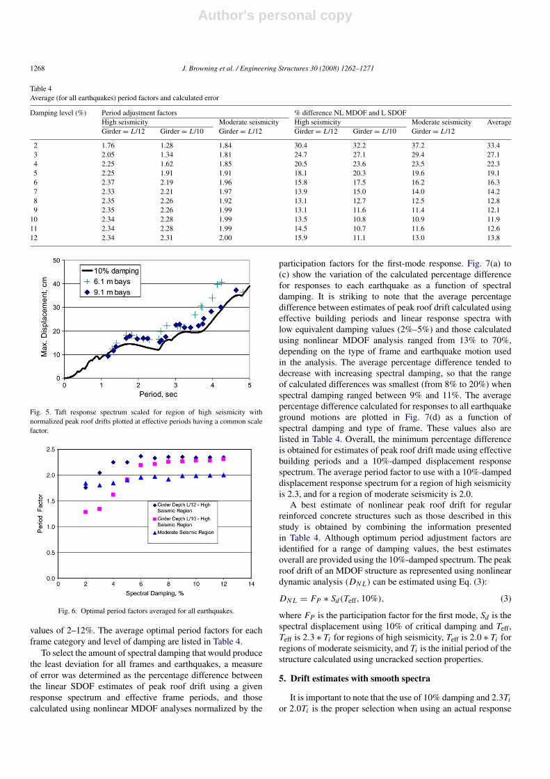
Fig. 5 shows the results of an optimization for the framesproportioned for a region of high seismicity and subjected tothe Taft ground motion. The normalized peak roof drifts areplotted at the frame effective periods, which are the initialperiods multiplied by a common period factor that producedthe best “fit” as described above. In this case, the 10%-dampedTaft spectrum was identified, and the effective periods used inFig. 5 are the initial periods factored by 2.12. This procedurewas repeated for each set of frames (proportioned for moderateor high seismicity), earthquake ground motion, and responsespectrum of a given damping level.

Fig. 6 shows the optimal period factors for each framecategory, averaged for all earthquake ground motions, andplotted as a function of spectral damping. In general, the periodfactor increases as the spectral damping increases to a valueof 6%, after which it remains nearly constant. For the framesproportioned for a region of moderate seismicity the factors didnot vary greatly, ranging from 1.8 to 2.0 for spectral damping

Author's personal copy

1268 J. Browning et al. / Engineering Structures 30 (2008) 1262–1271

Table 4Average (for all earthquakes) period factors and calculated error

Damping level (%) Period adjustment factors % difference NL MDOF and L SDOFHigh seismicity Moderate seismicity High seismicity Moderate seismicity AverageGirder = L/12 Girder = L/10 Girder = L/12 Girder = L/12 Girder = L/10 Girder = L/12

2 1.76 1.28 1.84 30.4 32.2 37.2 33.43 2.05 1.34 1.81 24.7 27.1 29.4 27.14 2.25 1.62 1.85 20.5 23.6 23.5 22.35 2.25 1.91 1.91 18.1 20.3 19.6 19.16 2.37 2.19 1.96 15.8 17.5 16.2 16.37 2.33 2.21 1.97 13.9 15.0 14.0 14.28 2.35 2.26 1.92 13.1 12.7 12.5 12.89 2.35 2.26 1.99 13.1 11.6 11.4 12.1

10 2.34 2.28 1.99 13.5 10.8 10.9 11.911 2.34 2.28 1.99 14.5 10.7 11.6 12.612 2.34 2.31 2.00 15.9 11.1 13.0 13.8

Fig. 5. Taft response spectrum scaled for region of high seismicity withnormalized peak roof drifts plotted at effective periods having a common scalefactor.

Fig. 6. Optimal period factors averaged for all earthquakes.

values of 2–12%. The average optimal period factors for eachframe category and level of damping are listed in Table 4.

To select the amount of spectral damping that would producethe least deviation for all frames and earthquakes, a measureof error was determined as the percentage difference betweenthe linear SDOF estimates of peak roof drift using a givenresponse spectrum and effective frame periods, and thosecalculated using nonlinear MDOF analyses normalized by the

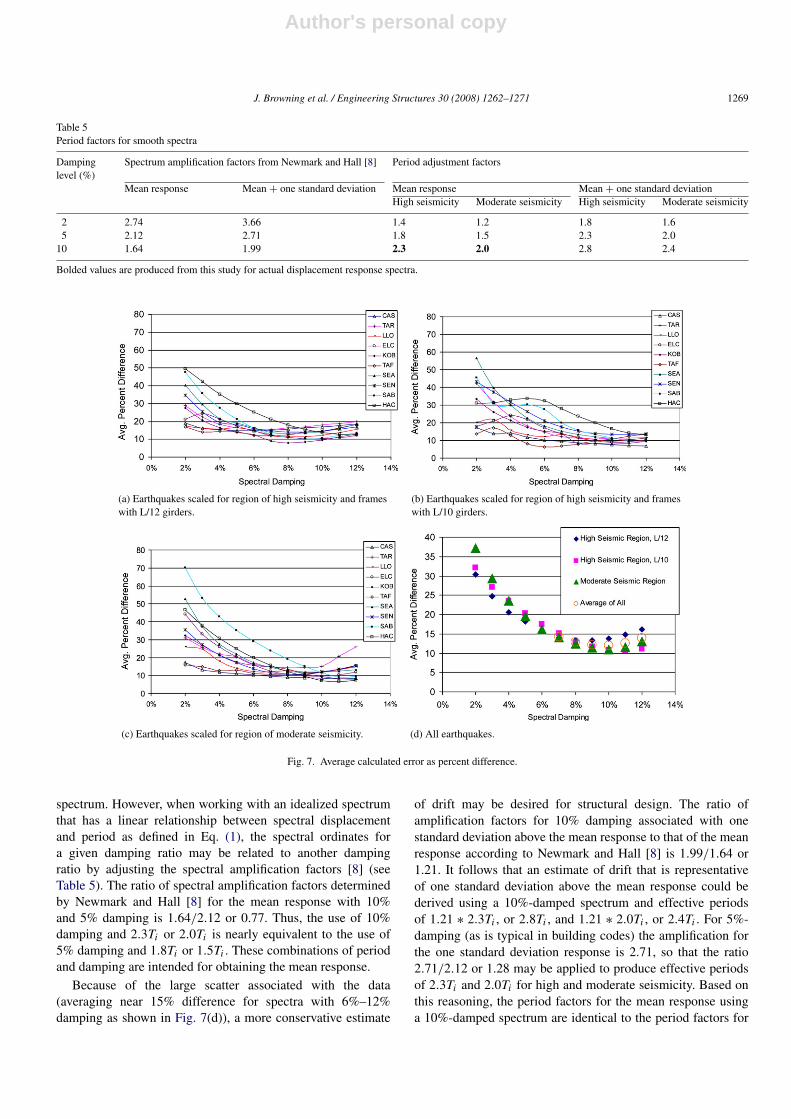
participation factors for the first-mode response. Fig. 7(a) to(c) show the variation of the calculated percentage differencefor responses to each earthquake as a function of spectraldamping. It is striking to note that the average percentagedifference between estimates of peak roof drift calculated usingeffective building periods and linear response spectra withlow equivalent damping values (2%–5%) and those calculatedusing nonlinear MDOF analysis ranged from 13% to 70%,depending on the type of frame and earthquake motion usedin the analysis. The average percentage difference tended todecrease with increasing spectral damping, so that the rangeof calculated differences was smallest (from 8% to 20%) whenspectral damping ranged between 9% and 11%. The averagepercentage difference calculated for responses to all earthquakeground motions are plotted in Fig. 7(d) as a function ofspectral damping and type of frame. These values also arelisted in Table 4. Overall, the minimum percentage differenceis obtained for estimates of peak roof drift made using effectivebuilding periods and a 10%-damped displacement responsespectrum. The average period factor to use with a 10%-dampeddisplacement response spectrum for a region of high seismicityis 2.3, and for a region of moderate seismicity is 2.0.

A best estimate of nonlinear peak roof drift for regularreinforced concrete structures such as those described in thisstudy is obtained by combining the information presentedin Table 4. Although optimum period adjustment factors areidentified for a range of damping values, the best estimatesoverall are provided using the 10%-damped spectrum. The peakroof drift of an MDOF structure as represented using nonlineardynamic analysis (DN L) can be estimated using Eq. (3):

DN L = FP ∗ Sd(Teff, 10%), (3)

where FP is the participation factor for the first mode, Sd is thespectral displacement using 10% of critical damping and Teff,Teff is 2.3 ∗ Ti for regions of high seismicity, Teff is 2.0 ∗ Ti forregions of moderate seismicity, and Ti is the initial period of thestructure calculated using uncracked section properties.

5. Drift estimates with smooth spectra

It is important to note that the use of 10% damping and 2.3Tior 2.0Ti is the proper selection when using an actual response

Author's personal copy

J. Browning et al. / Engineering Structures 30 (2008) 1262–1271 1269

Table 5Period factors for smooth spectra

Dampinglevel (%)

Spectrum amplification factors from Newmark and Hall [8] Period adjustment factors

Mean response Mean + one standard deviation Mean response Mean + one standard deviationHigh seismicity Moderate seismicity High seismicity Moderate seismicity

2 2.74 3.66 1.4 1.2 1.8 1.65 2.12 2.71 1.8 1.5 2.3 2.0

10 1.64 1.99 2.3 2.0 2.8 2.4

Bolded values are produced from this study for actual displacement response spectra.

(a) Earthquakes scaled for region of high seismicity and frameswith L/12 girders.

(b) Earthquakes scaled for region of high seismicity and frameswith L/10 girders.

(c) Earthquakes scaled for region of moderate seismicity. (d) All earthquakes.

Fig. 7. Average calculated error as percent difference.

spectrum. However, when working with an idealized spectrumthat has a linear relationship between spectral displacementand period as defined in Eq. (1), the spectral ordinates fora given damping ratio may be related to another dampingratio by adjusting the spectral amplification factors [8] (seeTable 5). The ratio of spectral amplification factors determinedby Newmark and Hall [8] for the mean response with 10%and 5% damping is 1.64/2.12 or 0.77. Thus, the use of 10%damping and 2.3Ti or 2.0Ti is nearly equivalent to the use of5% damping and 1.8Ti or 1.5Ti . These combinations of periodand damping are intended for obtaining the mean response.

Because of the large scatter associated with the data(averaging near 15% difference for spectra with 6%–12%damping as shown in Fig. 7(d)), a more conservative estimate

of drift may be desired for structural design. The ratio ofamplification factors for 10% damping associated with onestandard deviation above the mean response to that of the meanresponse according to Newmark and Hall [8] is 1.99/1.64 or1.21. It follows that an estimate of drift that is representativeof one standard deviation above the mean response could bederived using a 10%-damped spectrum and effective periodsof 1.21 ∗ 2.3Ti , or 2.8Ti , and 1.21 ∗ 2.0Ti , or 2.4Ti . For 5%-damping (as is typical in building codes) the amplification forthe one standard deviation response is 2.71, so that the ratio2.71/2.12 or 1.28 may be applied to produce effective periodsof 2.3Ti and 2.0Ti for high and moderate seismicity. Based onthis reasoning, the period factors for the mean response usinga 10%-damped spectrum are identical to the period factors for

Author's personal copy

1270 J. Browning et al. / Engineering Structures 30 (2008) 1262–1271

the one standard deviation above the mean response using a5%-damped spectrum, as shown in Table 5.

6. Magnitude and location of maximum story distortion

In the absence of a story mechanism, peak roof drift(global response) is a good indicator of the average distortiona building structure must withstand for a given earthquakedemand. The adequacy of a design, however, is directlytied to local deformations typically measured by story drifts.Building codes and design guidelines, such as those providedby ASCE 7 [14], limit the calculated story drift to controldistortions, and therefore damage, to the structural elements andbuilding contents. Depending on the Occupancy Category forthe structure, an allowable story drift for an RC building mayvary between 1.0% and 2.5% of the story height. It is of interestto determine how the location and magnitude of calculated storydrift using linear analysis compares with that calculated usingnonlinear analysis.

The maximum story drift ratios (ratio of maximum storydrift to story height) were determined from each nonlineardynamic analysis of the frames proportioned for a region ofhigh seismicity and having girders with depths equal to one-twelfth the span length. These frames were selected becausethey had more elements that yielded during response andgreater rotation demands. In addition to nonlinear analysis,the maximum story drift ratios were calculated based onlinear analysis using the square-root-sum-of-the-squares modalcombination method with the first three modes of vibration. Thenonlinear and linear analyses performed to compare story driftswere based on 2% damping proportional to the initial stiffness.

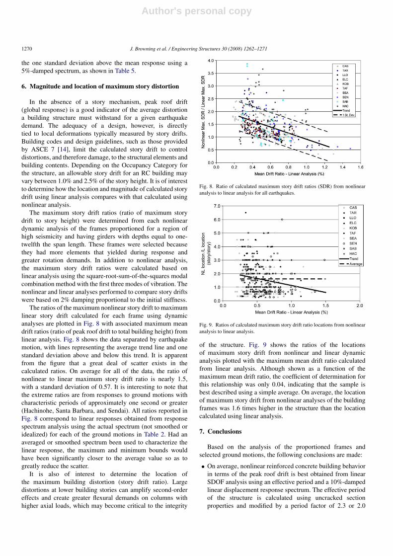
The ratios of the maximum nonlinear story drift to maximumlinear story drift calculated for each frame using dynamicanalyses are plotted in Fig. 8 with associated maximum meandrift ratios (ratio of peak roof drift to total building height) fromlinear analysis. Fig. 8 shows the data separated by earthquakemotion, with lines representing the average trend line and onestandard deviation above and below this trend. It is apparentfrom the figure that a great deal of scatter exists in thecalculated ratios. On average for all of the data, the ratio ofnonlinear to linear maximum story drift ratio is nearly 1.5,with a standard deviation of 0.57. It is interesting to note thatthe extreme ratios are from responses to ground motions withcharacteristic periods of approximately one second or greater(Hachinohe, Santa Barbara, and Sendai). All ratios reported inFig. 8 correspond to linear responses obtained from responsespectrum analysis using the actual spectrum (not smoothed oridealized) for each of the ground motions in Table 2. Had anaveraged or smoothed spectrum been used to characterize thelinear response, the maximum and minimum bounds wouldhave been significantly closer to the average value so as togreatly reduce the scatter.

It is also of interest to determine the location ofthe maximum building distortion (story drift ratio). Largedistortions at lower building stories can amplify second-ordereffects and create greater flexural demands on columns withhigher axial loads, which may become critical to the integrity

Fig. 8. Ratio of calculated maximum story drift ratios (SDR) from nonlinearanalysis to linear analysis for all earthquakes.

Fig. 9. Ratios of calculated maximum story drift ratio locations from nonlinearanalysis to linear analysis.

of the structure. Fig. 9 shows the ratios of the locationsof maximum story drift from nonlinear and linear dynamicanalysis plotted with the maximum mean drift ratio calculatedfrom linear analysis. Although shown as a function of themaximum mean drift ratio, the coefficient of determination forthis relationship was only 0.04, indicating that the sample isbest described using a simple average. On average, the locationof maximum story drift from nonlinear analyses of the buildingframes was 1.6 times higher in the structure than the locationcalculated using linear analysis.

7. Conclusions

Based on the analysis of the proportioned frames andselected ground motions, the following conclusions are made:

• On average, nonlinear reinforced concrete building behaviorin terms of the peak roof drift is best obtained from linearSDOF analysis using an effective period and a 10%-dampedlinear displacement response spectrum. The effective periodof the structure is calculated using uncracked sectionproperties and modified by a period factor of 2.3 or 2.0

Author's personal copy

J. Browning et al. / Engineering Structures 30 (2008) 1262–1271 1271

for frames proportioned in regions of high or moderateseismicity, respectively.

• Because of the high scatter involved in estimating nonlinearstructural drift with linear response spectra, conservativeestimates for design should be obtained using a smooth5%-damped spectrum and a period factor (ratio of effectiveperiod to initial period) of 2.3 or 2.0 for frames proportionedin regions of high or moderate seismicity, respectively.

• The location of maximum distortion calculated using MDOFnonlinear dynamic analysis of reinforced concrete frames is,on average, 60% higher in the structure than that calculatedusing linear modal analysis.

• On average, the magnitude of the maximum story driftratio calculated using nonlinear analysis is a factor of1.5 larger than that estimated using linear modal analysis.The coefficient of variation is 0.39 for these calculatedratios, with larger deviations from the average value forthose systems responding to earthquake motions havingcharacteristic periods exceeding one second.

References

[1] Gulkan P, Sozen M. Inelastic response of reinforced concrete structuresto earthquakes motions. ACI Journal 1974;71:604–10.

[2] Shibata A, Sozen M. Substitute-structure method for seismic design inR/C. Journal of Structural Division, ASCE 1976;102:1–18.

[3] Shimazaki K, Sozen M. Seismic drift of reinforced concrete structures.Technical research report of Hazama-Gumi, Ltd. 1984. p. 145–66.

[4] Lepage A. A method for drift-control in earthquake-resistant design ofRC building structures. Doctoral thesis. University of Illinois at Urbana-Champaign. 1997.

[5] Iwan WD, Gates NC. The effective period and damping of a class ofhysteretic structures. Earthquake Engineering and Structural Dynamics1979;8:199–211.

[6] Iwan WD. Estimating inelastic response spectra from elastic spectra.Earthquake Engineering and Structural Dynamics 1980;8:375–88.

[7] Iwan WD, Guyader AC. A study of the accuracy of the capacityspectrum method in engineering analysis. In: Proceedings of the 3rd USJapan workshop on performance-based earthquake eng. methodology forreinforced concrete building structures (PEER). 2002. p. 86–102.

[8] Newmark N, Hall W. Earthquake spectra and design. EERI monographseries. Oakland (CA): Earthquake Engineering Research Institute; 1982.

[9] Ruiz-Garcia J, Miranda E. Inelastic displacement ratios for evaluationof existing structures. Earthquake Engineering and Structural Dynamics2003;32(8):1237–58.

[10] Kowalsky MJ, Priestley MN, MacRae GA. Displacement-based design,a methodology for seismic design applied to SDOF reinforced concretestructures. Structural system research project, Report SSRP-94/16. SanDiego and La Jolla (CA): University of California; 1994.

[11] Priestley MN, Kowalsky MJ. Direct displacement-based seismic design ofconcrete buildings. Bulletin of the New Zealand Society for Earthquake

Engineering 2000;33:421–44.[12] Matamoros A, Garcia LE, Browning J, Lepage A. Flat-rate design method

for low- and medium-rise reinforced concrete structures. ACI StructuralJournal 2004;101(4):435–46.

[13] International Code Council. International building code. IL: Country ClubHills; 2006.

[14] ASCE/SEI 7-05. Minimum design loads for buildings and otherstructures. Reston (VA): American Society of Civil Engineers; 2006.

[15] Browning J. Proportioning of earthquake-resistant reinforced concretebuilding structures. Thesis submitted in partial fulfillment of therequirements for the degree of Ph.D. in Civil Engineering. West Lafayette(IN): Purdue University; 1998.

[16] Otani S. SAKE: A computer program for inelastic response of R/C framesto earthquakes. Structural research series No. 413. Urbana (IL): CivilEngineering Studies, University of Illinois; 1974.

[17] Saiidi M, Sozen MA. Simple and complex models for nonlinear seismicresponse of reinforced concrete structures. Structural research seriesNo. 465. Urbana (IL): Civil Engineering Studies, University of Illinois;1979.

[18] Lopez R. Numerical model for nonlinear response of R/C frame-wall structures. Ph.D. thesis submitted to the Graduate College of theUniversity of Illinois. Urbana (IL): 1988.

[19] Browning J, Li R, Lynn A, Moehle JP. Performance assessment fora reinforced concrete frame building. Earthquake Spectra 2000;16(3):541–55.

[20] Hognestad E. A study of combined bending and axial load in reinforcedconcrete members. Bulletin series No. 399. Urbana (IL): University ofIllinois Engineering Experiment Station; 1951.

[21] Takeda T, Sozen M, Nielsen N. Reinforced concrete response to simulatedearthquakes. Journal of the Structural Division, ASCE 1970;96(ST12):2557–73.

[22] CALTECH. Strong motion earthquake accelerograms, digitized andplotted data, vol. II-D. Report EERL No. 72-52. Pasadena (CA):Earthquake Engineering Research Laboratory, California Institute ofTechnology; 1973.

[23] CSMIP. Processed CSMIP strong-motion records from the Northridge.California, Earthquake of 17 January 1994, Release No. 1 through ReleaseNo. 7. Report no. OSMS 94-06 through 94-12. California Department ofConservation, Division of Mines and Geology, Office of Strong-MotionStudies. Sacramento (CA); 1994.

[24] Saragoni R, Gonzalez P, Fresard M. Analisis de los Acelerogramas delTerremoto del 3 de Marzo de 1985. Publicacion SES-I-4/1985(199).Universidad de Chile; 1985.

[25] CALTECH. Strong motion earthquake accelerograms. Digitized andplotted data, vol. II-A. Report EERL No. 71-50. Pasadena (CA):Earthquake Engineering Research Laboratory, California Institute ofTechnology; 1971.

[26] JMA. Strong motion accelerograms. Japan Meteorological Agency; 1995.[27] CALTECH. Strong motion earthquake accelerograms, digitized and

plotted data, vol. II-B. Report EERL No. 72-50. Pasadena (CA):Earthquake Engineering Research Laboratory, California Institute ofTechnology; 1973.

[28] Mori AW, Crouse CB. Strong motion data from japanese earthquakes.Report SE-29. Boulder (CO): National Geophysical Data Center, NationalOceanic and Atmospheric Administration; 1981.