fundamentals of plastic optical fibers

Yasuhiro Koike

Fundamentals of Plastic Optical Fibers

Related Titles

Schnabel, W.

Polymers and Electromagnetic

Radiation

Fundamentals and Practical Applications

2014

ISBN: 978-3-527-33607-4

Also available in digital formats

Nicolais, L., Carotenuto, G. (eds.)

NanocompositesIn Situ Synthesis of Polymer-Embedded

Nanostructures

2014

ISBN: 978-0-470-10952-6

Reed, G.T. (ed.)

Silicon Photonics - The State of

the Art

2008

ISBN: 978-0-470-99453-5

Hadziioannou, G., Malliaras, G.G. (eds.)

Semiconducting Polymers

Chemistry, Physics and Engineering

Second Edition

2007

ISBN: 978-3-527-31271-9

Schnabel, W.

Polymers and LightFundamentals and Technical

Applications

2007

ISBN: 978-3-527-31866-7

Also available in digital formats

Steinbüchel, A. (ed.)

Biopolymers

10 Volumes + Index

2003

ISBN: 978-3-527-30290-1

Iizuka, K.

Elements of Photonics,

2-Volume Set

2002

ISBN: 978-0-471-41115-4

Saleh, B.E., Teich, M.C.

Fundamentals of Photonics

1991

ISBN: 978-0-471-83965-1

Yasuhiro Koike

Fundamentals of Plastic Optical Fibers

The Author

Yasuhiro Koike

Professor, Keio University

Director, Keio Photonics Research

Institute

Yokohama, Japan

Cover

The picture represents how light prop-

agates through graded index POFs. The

incident light draws a sine curve because

GI POFs have parabolic refractive index

profiles in the core regions.

All books published by Wiley-VCH are

carefully produced. Nevertheless, authors,

editors, and publisher do not warrant the

information contained in these books,

including this book, to be free of errors.

Readers are advised to keep in mind that

statements, data, illustrations, procedural

details or other items may inadvertently

be inaccurate.

Library of Congress Card No.: applied for

British Library Cataloguing-in-Publication

Data

A catalogue record for this book is

available from the British Library.

Bibliographic information published by the

Deutsche Nationalbibliothek

The Deutsche Nationalbibliothek

lists this publication in the Deutsche

Nationalbibliografie; detailed

bibliographic data are available on the

Internet at http://dnb.d-nb.de.

© 2015 Wiley-VCH Verlag GmbH & Co.

KGaA, Boschstr. 12, 69469 Weinheim,

Germany

All rights reserved (including those of

translation into other languages). No part

of this book may be reproduced in any

form – by photoprinting, microfilm,

or any other means – nor transmitted

or translated into a machine language

without written permission from the

publishers. Registered names, trademarks,

etc. used in this book, even when not

specifically marked as such, are not to be

considered unprotected by law.

Print ISBN: 978-3-527-41006-4

ePDF ISBN: 978-3-527-64653-1

ePub ISBN: 978-3-527-64652-4

Mobi ISBN: 978-3-527-64651-7

oBook ISBN: 978-3-527-64650-0

Cover-Design Adam-Design, Weinheim,

Germany

Typesetting Laserwords Private Limited,

Chennai, India

Printing and Binding Markono Print

Media Pte Ltd., Singapore

Printed on acid-free paper

http://dnb.d-nb.de

V

Contents

Preface IX

Acknowledgments XIII

1 Introduction: Faster, Further, More Information 1

1.1 Principle of Optical Fiber 3

1.2 Plastic Optical Fiber 6

References 9

2 Transmission Loss 11

2.1 Absorption Loss 11

2.1.1 Electronic Transition Absorption 11

2.1.2 Molecular Vibration Absorption 12

2.1.3 Effect of Fluorination on Attenuation Spectra of POFs 15

2.2 Scattering Loss 19

2.2.1 Definition of Scattering Loss 19

2.2.2 Heterogeneous Structure and Excess Scattering 20

2.2.3 Origin of Excess Scattering in PMMA 21

2.2.4 Empirical Estimation of Scattering Loss for Amorphous

Polymers 23

2.3 Low-Loss POFs 26

2.3.1 PMMA- and PSt-Based POFs 26

2.3.2 PMMA-d8-Based POF 26

2.3.3 CYTOP®-Based POF 27

References 28

3 Transmission Capacity 31

3.1 Bandwidth 32

3.1.1 Intermodal Dispersion 32

3.1.2 Intramodal Dispersion 34

3.1.3 High-Bandwidth POF 35

3.2 Wave Propagation in POFs 38

3.2.1 Microscopic Heterogeneities 39

3.2.2 Debye’s ScatteringTheory 40

VI Contents

3.2.3 Developed Coupled PowerTheory 42

3.2.4 Mode Coupling Mechanism 44

3.2.5 Efficient Group Delay Averaging 46

3.3 Mode Coupling Effect in POFs 50

3.3.1 Radio-over-Fiber with GI POFs 50

3.3.2 Noise Reduction Effect in GI POFs 50

References 55

4 Materials 59

4.1 Representative Base Polymers of POFs 59

4.1.1 Poly(methyl methacrylate) 59

4.1.2 Perfluorinated Polymer, CYTOP® 61

4.2 Partially Halogenated Polymers 63

4.2.1 Polymethacrylate Derivatives 63

4.2.2 Polystyrene Derivatives 67

4.3 Perfluoropolymers 70

4.3.1 Perfluorinated Polydioxolane Derivatives 70

4.3.2 Copolymers of Dioxolane Monomers 74

4.3.3 Copolymers of Perfluoromethylene Dioxolanes and Fluorovinyl

Monomers 74

References 76

5 Fabrication Techniques 79

5.1 Production Processes of POFs 79

5.1.1 Preform Drawing 79

5.1.2 Batch Extrusion 80

5.1.3 Continuous Extrusion 81

5.2 Fabrication Techniques of Graded-Index Preforms 82

5.2.1 Copolymerization 82

5.2.1.1 Binary Monomer System 84

5.2.1.2 Ternary Monomer System 85

5.2.2 Preferential Dopant Diffusion 90

5.2.3 Thermal Dopant Diffusion 91

5.2.4 Polymerization under Centrifugal Force 93

5.3 Extrusion of GI POFs 95

References 98

6 Characterization 101

6.1 Refractive Index Profile 101

6.1.1 Power-Law Approximation 101

6.1.2 Transverse Interference Technique 102

6.2 Launching Condition 105

6.2.1 Underfilled and Overfilled Launching 106

6.2.2 Differential Mode Launching 107

6.3 Attenuation 107

Contents VII

6.3.1 Cutback Technique 108

6.3.2 Differential Mode Attenuation 110

6.4 Bandwidth 111

6.4.1 Time Domain Measurement 112

6.4.2 Differential Mode Delay 113

6.5 Near-Field Pattern 114

References 117

7 Optical Link Design 119

7.1 Link Power Budget 120

7.2 Eye Diagram 120

7.2.1 Eye Opening 121

7.2.2 Eye Mask 122

7.3 Bit Error Rate and Link Power Penalty 122

7.3.1 Intersymbol Interference 125

7.3.2 Extinction Ratio 126

7.3.3 Mode Partition Noise 126

7.3.4 Relative Intensity Noise 127

7.4 Coupling Loss 127

7.4.1 Core Diameter Dependence 128

7.4.2 Ballpoint Pen Termination 129

7.4.3 Ballpoint Pen Interconnection 132

7.5 Design for Gigabit Ethernet 134

References 135

Appendix Progress in Low-Loss and High-Bandwidth Plastic Optical Fibers 139

A.1 Introduction 139

A.2 Basic Concept and Classification of Optical Fibers 140

A.3 The Advent of Plastic Optical Fibers and Analysis of

Attenuation 143

A.3.1 Absorption Loss 144

A.3.2 Scattering Loss 147

A.4 Graded-Index Technologies for Faster Transmission 149

A.4.1 Interfacial-Gel Polymerization Technique 150

A.4.2 Coextrusion Process 152

A.5 Recent Studies of Low-Loss and Low-Dispersion Polymer

Materials 153

A.5.1 Partially Fluorinated Polymers 156

A.5.2 Perfluorinated Polymer 159

A.6 Conclusion 165

Acknowledgment 165

References 166

Index 169

IX

Preface

People in the industry formerly held the vague notion that polymers were

unsuitable for application in the high-performance photonics field. Twenty odd

years later, however, we have seen the birth of photonic polymers in applications

such as the world’s fastest plastic optical fiber (POF) and high-resolution displays.

Research papers written in the first half of the twentieth century by Einstein and

Debye, which delve into the essence of light scattering, have become my personal

bibles. From them, I learned that the more we strive to achieve a breakthrough,

the more important it is that we return to the fundamentals.

What originally drew me into the academic field of photonic polymers, a field

which combines photonics and physical sciences, was my meeting with the late

Professor Yasuji Otsuka, a personwho I have the greatest respect for. I was a fourth

year undergraduate student when I joined Professor Otsuka’s laboratory in 1976.

At that time, the laboratory had just begun its research into optically converg-

ing plastic rod lenses. By creating a graded index (GI) in the radial direction in

a rod-shaped polymer, the light passing through it would travel in a meander-

ing path, forming an image even when both ends of the rod were flat. I found

this to be a most curious phenomenon and became fascinated by polymers. What

interested me at first was why a GI causes light to bend gradually according to

the refractive index profile. Professor Otsuka was an expert in polymer chemistry,

focusing on emulsion polymerization, but he worked out and explainedMaxwell’s

ray equation to me. I was very impressed and also surprised at the fact that he had

gone beyond his particular field of polymer chemistry and was attempting to use

optics and mathematics to explain the behavior of light in a polymer. I greatly

admired Professor Otsuka.

Years later, I would find myself researching the fundamental reasons for light

scattering loss – the prime reason why fibers could not be made transparent.

While I remained a member of the polymer chemistry laboratory, on my own

I entered the worlds of physics and optics as I studied subjects such as light

scattering theory and polarization. I would continue to learn in the academic

field of photonic polymers for the next 20 years, but my fundamental research

method was the one that I learned at that time from Professor Otsuka.

In 1982, I received Ph.D. from Keio University and I was at a crossroads in my

research into the question of whether it was truly possible to create a GI-type POF

X Preface

that could transmit optical signals at speeds exceeding one gigabit. The prototype

GI-POF suffered from low transparency, and had a transmission loss of more than

1000 dB/km, preventing the light from traveling farther than a fewmeters. In order

to achieve transmission speeds exceeding one gigabit, it was necessary to create a

GI by adding another material inside the fiber and creating a density distribution

in the radial direction. However, at the same time, determining how to eliminate

impurities in order to make the POF transparent was a major issue. Therefore,

attempting to achieve high-speed optical communication by adding anothermate-

rial (an impurity?) that would create a GI was a large challenge.

At that time, in order to create a gradient index, twomonomersM1 andM2with

different reactivities were copolymerized. A polymer containing large quantities

of the highly polymerizable M1 monomer with its low refractive index was grad-

ually deposited around the periphery to create the gradient index.The created GI

preform appeared transparent, but it was possible to see the light beam traveling in

a prettymeandering path whichwas visible as a result of scattering of the light.We

needed to reduce this light scattering loss by a factor of at least several hundreds.

I was completely unaware of the large and theoretically impenetrable barrier

which lays in the way of continuously improving the copolymerzation method

which uses the different reactivities of the monomers to create the gradient index,

and I continued to work toward creating a transparent GI-POF.

The problem of light scattering consumed me, and I was not able to assign this

as a research theme for student graduation or master’s theses because I did not

know whether the research would produce any results. I continued to struggle

with the problem on my own. As I was reading a broad range of documents on

the subject, I came across Einstein’s fluctuation theory of light scattering from the

early twentieth century. This was based on micro-Brownian motion in solution,

and it proposes that light scattering loss is proportional to isothermal compress-

ibility. When I actually entered the isothermal compressibility of the POF mate-

rial PMMA (poly(methyl methacrylate)), I obtained a value of 10 dB/km – much

lower than the aforementioned value of 1000 dB/km. This meant that transmis-

sion over a distance exceeding 1 km was possible. This was truly a revelation to

me at that time. However, in that case, where did the difference of 990 dB/km

come from? In order to identify the kind of heterogeneous structure which was

producing this excessive scattering, I learned everything I could about light scat-

tering usingDebye’s correlation function from the 1950s. I also tried again to work

the theory out on my own. This was an extremely useful theory for quantitative

analysis of the relationship between micro nonuniform polymer structures and

light scattering. What was wonderful about Debye’s scattering theory was that it

was possible to define the correlation function without hypothesizing the shape or

size of the heterogeneous structures in the polymer chain. This makes it possible

to experimentally find the correlation distance that includes information about the

heterogeneous structure shape and size from the angular dependence of the light

scattering. This became a powerful tool for me in working to identify the cause of

excess polymer scattering.

Preface XI

At the same time, I began to see how the method of forming a gradient index

according to differences in reactivity would form an extreme polymer composi-

tional distribution in the generated copolymer. It became clear that, as we tried

to make the gradient index larger by increasing the difference in reactivity, the

polymer compositionwould contain increasing amounts of components that were

similar to homopolymers ofM1 andM2.This essential large heterogeneous struc-

ture reached sizes in excess of several hundred angstroms, and when applied to

Debye’s light-scattering theory, I discovered it to be the cause of an enormously

large scattering loss exceeding several hundred decibels per kilometer. This real-

ization was the culmination of many long years of research and allowed me to

recognize that the fiber would theoretically not become transparent utilizing pro-

cessing methods that rely on monomer reactivity.

I began experiments based on the completely new idea of forming a gradient

index using the sizes of the molecules instead of the monomer reactivity. I still

remember the day very clearly. It was April 1, 1990 (April Fool’s Day). On that day,

I had produced a superbly transparent GI-POF preform. This was the moment

I emerged from my 10-year-long search for a solution to scattering loss. Our lab-

oratory was galvanized from this point on. Our course was clearly set, and all

student research themes were channeled in this direction. Test data on GI-POF

with increasingly lower losses and higher speeds were produced one after another.

I obtained a patent, wrote numerous papers, and began joint research with indus-

try all at once. News that an optical signal with speed exceeding a gigabit passed

through 100m of GI-POF for the first time was reported on August 31, 1994, on

the front page of the Nikkei Shimbun (newspaper).

The production method up until around 2005 was the preformmethod (a man-

ufacturing method where a GI preform is created, which is then made into GI-

POF through heat-drawing) with a focus on the interfacial-gel polymerization

method. However, from around 2005, we began to develop the continuous extru-

sion method in earnest, and by 2008 succeeded in 40-Gb transmission. This was

the world’s fastest transmission speed, surpassing the GI-type silica optical fiber.

We achieved these results through joint research with Asahi Glass. It was based

on the essential principle of the materials, which indicates that a perfluorinated

polymer used as the POF core material has a lower material dispersion compared

to silica. (Material dispersion determines the transmission bandwidth.)

My research into light scattering, which I have described here, has been sup-

ported by the research papers that were written by Einstein and Debye during the

first half of the twentieth century, and which delve into the essence of light scat-

tering. Through these papers, I realized that the latest research papers would not

always be useful in pursuing leading-edge research. I learned that the more we

strive to achieve a breakthrough, the more important it is that we return to the

fundamentals.

Yasuhiro Koike

XIII

Acknowledgments

This book was written by Yasuhiro Koike with inputs from Kenji Makino

(Chapters 1, 3, 6, and 7), Azusa Inoue (Chapters 2 and 3), and Kotaro Koike

(Chapters 2, 4, and 5), Project Assistant Professors of Keio Photonics Research

Institute, Keio University, Japan. Their works were supported by the Japan

Society for the Promotion of Science (JSPS) through its “Funding Program for

World-Leading Innovative R&D on Science and Technology” (FIRST Program).

1

1

Introduction: Faster, Further, More Information

The realization of these three features has motivated the development of commu-

nication systems since the dawn of history. Optical communication systems in the

broad sense date back to ancient times. One of the earliest optical communication

systems was fire and smoke. Although atmospheric conditions, such as rain, snow,

fog, and dust, strongly affect the transmission reliability, this type of optical com-

munication was used for a long time worldwide. In addition to the sensitivity to

the environmental conditions, the signal receiver was the human eye; thus, the

transmission system had poor reliability. More stable and dependable communi-

cation systems were developed; for instance, a courier or pigeon carried messages

and letters.

The era of electrical communication started in 1837 with the invention of the

telegraph by Samuel F. B.Morse.The telegraph systemused theMorse code, which

represents letters and numbers by a coded combination of dots and dashes. The

encoded symbols were conveyed by sending short and long pulses of electricity

over a copper wire at a rate of tens of pulses per second.The telegraph andMorse

code dramatically improved the speed, quality, and information capacity of trans-

mission, although well-trained and skilled operators were required.

Another giant leap in the history of communication systems was brought about

by Alexander Graham Bell in 1876. Bell developed a fundamentally different and

user-friendly device that could transmit the entire voice as is, in an analog signal.

The device is the telephone, which rapidly increased the speed and quality of

communication. Subsequently, the invention of the facsimile machine enabled

the transmission of figures and drawings. The development of electrical commu-

nication systems shifted to use progressively higher frequencies, which offered

increases in bandwidth or information capacity. Optical communication was

gradually becoming attractive because optical frequencies are several orders of

magnitude higher than those used by electrical communication systems. There-

fore, the optical carrier frequencies yield a far greater potential transmission

bandwidth than electrical systems with metallic cables.

No significant advance in optical communication appeared until the invention

of the laser in the early 1960s because no practical transmitter existed, and all

communication systems must include the fundamental elements of a transmitter,

the transmission medium, and a receiver. The invention of the laser aroused

Fundamentals of Plastic Optical Fibers, First Edition. Yasuhiro Koike.© 2015 Wiley-VCH Verlag GmbH & Co. KGaA. Published 2015 by Wiley-VCH Verlag GmbH & Co. KGaA.

2 1 Introduction: Faster, Further, More Information

curiosity about the possibility of using the optical wavelength region of the

electromagnetic spectrum for transmission systems. The optical frequencies

generated by such a coherent optical source are on the order of 1014 Hz, and

the laser theoretically has an information capacity exceeding that of microwave

systems by a factor of 105. Experimental investigations using atmospheric

optical channels were conducted in the early 1960s with the potential of such

broadband transmission capacities in mind. However, the transmission quality

was unstable, again depending on the atmospheric conditions. At the same time,

it was recognized that an optical fiber can provide a more reliable transmission

channel because it is immune to environmental conditions [1]. The initial optical

fibers appeared impractical because of their extremely large optical losses of

more than 1000 dB/km. The situation changed in 1966, when Kao and Hockham

speculated that the high losses were a result of impurities in the fiber material,

and that the losses could potentially be reduced significantly in order to make

optical fibers a functional transmission medium [2]. The technical breakthrough

for optical communication occurred in 1970, only 4 years after this prediction; an

optical fiber was demonstrated with a purified silica glass having an optical power

loss low enough for a practical transmission link [3]. Charles K. C. Kao won the

Nobel Prize in physics in 2009 for his pioneering insight and his enthusiastic

further development of low-loss optical fibers. Ultimately, these efforts resulted

in practical optical communication systems widely used across the earth. Optical

fiber systems commonly provide great advantages such as longer distance, greater

information capacity, immunity to electromagnetic interference, information

security, smaller size, and lighter weight. Applications for these sophisticated

networks include web browsing, e-mail exchange, telemedical care, remote

education, and grid and cloud computing.

The telecommunication industries seriously considered standardizing on mul-

timode fibers (MMFs) before deciding to adopt single-mode fibers (SMFs; see

the next section). MMFs are very attractive because the mechanical tolerances of

link components, such as connectors, splices, and coupling optics, are remarkably

relaxed compared to those of SMFs. However, MMFs were considered unsuitable

for telecommunication systems in the final analysis because of two critical tech-

nical problems: modal noise, and unstable bandwidth performance. Modal noise

is attributed to fluctuation in time of the speckle pattern resulting from interfer-

ence between the propagating modes, and bandwidth instability arises from the

central dip in the refractive index. In contrast, plastic optical fibers (POFs) have

an enormous number of propagating modes, and hence speckle patterns, which

practically cancel the modal noise effect by averaging the fluctuations. POFs have

essentially no central dip because of fabrication processes. Thus, serious modal

noise and unstable bandwidth have not been observed, even though POFs are

MMFs.Therefore, because the large mechanical tolerance provides easy and cost-

effective installation, MMFs, particularly POFs, have become attractive again and

have gradually been installed in short-reach networks such as local area networks

(LANs) in homes, offices, hospitals, and vehicles, and even very short-reach net-

works such as interconnects inside computers which contain many connections.


This chapter briefly describes the fundamentals of optical fibers and provides

an introductory review of the development of POFs.

1.1

Principle of Optical Fiber

Theprinciple of light propagation through optical fibers is simply explained as fol-

lows [4, 5]. An optical fiber generally consists of two coaxial layers in cylindrical

form: a core in the central part of the fiber and a cladding in the peripheral part

that completely surrounds the core. Although the cladding is not required for light

propagation in principle, it plays important roles in practical use, such as protect-

ing the core surface from imperfections and refractive index changes caused by

physical contact or contaminant absorption, and enhancement of the mechanical

strength. The core has a slightly higher refractive index than the cladding. There-

fore, when the incident angle of the light input to the core is greater than the crit-

ical angle determined by Snell’s law, the input light is confined to the core region

and propagates a long distance through the fiber because the light is repeatedly

reflected back into the core region by total internal reflection at the core–cladding

interface. The propagation of light along the fiber can be described in terms of

electromagnetic waves called modes, which are patterns of electromagnetic field

distributions. The fiber can guide a certain discrete number of modes that must

satisfy the electric and magnetic field boundary conditions at the core–cladding

interface according to its material and structure and the light wavelength.

Optical fibers can be commonly classified into two types: SMFs and MMFs [6].

As the names suggest, SMF allows only one propagating mode, whereas MMF

can guide a large number of modes. Both SMFs and MMFs are again divided into

two classes: step-index (SI) and graded-index (GI) fibers. The SI fiber has a con-

stant refractive index in the entire core. The refractive index changes abruptly

stepwise at the core–cladding boundary.TheGIfiber has a nearly parabolic refrac-

tive index distribution. The refractive index decreases gradually as a function of

the radial distance from the core center. Figure 1.1 conceptually illustrates the

refractive index profiles and ray trajectories in SMF and in SI and GI MMFs, and

shows the measured input and output pulse waveforms. The most significant dif-

ference among these types of fibers ismodal dispersion. Becausemodal dispersion

is described in detail in Chapter 3, the difference due to modal dispersion is only

briefly explained here.

When an optical pulse is input into an MMF, the optical power of the pulse is

generally distributed to a huge number of the modes of the fiber. Different modes

travel at different propagation speeds along the fiber, which means that different

modes launched at the same time reach the output end of the fiber at different

times. Therefore, the input pulse broadens in time as it travels along the MMF.

This pulse broadening effect, well known as modal dispersion, is significantly

observed in SI MMFs. As shown in Figure 1.1, different rays travel along paths

with different lengths; here each distinct ray can be thought of as a mode in a


Refractive index

profile

Refractive index

Refractive index

profile

Refractive index

Refractive index

profile

Refractive index

Input pulse

(a)

(b)

(c)

Meridional cross section and ray trajectory



Output pulse

through 100-m transmission

Output pulse


500 ps/div

500 ps-div

Output pulse


500 ps/div

500 ps/div

Input pulse500 ps/div

Input pulse500 ps/div

Figure 1.1 Refractive index profiles and ray trajectories in (a) SI SMF, (b) SI, and (c) GI

MMFs.

simple interpretation. The rays travel at the same velocity along their optical

paths because of the constant refractive index throughout the core region in an

SI MMF. Consequently, the same velocity and different path lengths result in

different propagation speeds along the fiber, which causes a wide pulse spread

in time. The pulse broadening caused by modal dispersion seriously limits the

transmission capacity of MMFs because overlapping of the broadened pulses

induces intersymbol interference and disrupts correct signal detection, thereby

increasing the bit error rate (see Chapter 7) [7].

Modal dispersion is generally a dominant factor in pulse broadening in MMFs.

However, modal dispersion can be dramatically reduced by forming a nearly

parabolic refractive index profile in the core region of a GI MMF, which allows

a much higher bandwidth and hence higher speed data transmission [8]. The

optical ray is confined to near the core axis, corresponding to a lower order mode,

and travels a shorter geometrical length at a slower light velocity along the path

because of the higher refractive index. The sinusoidal ray passing through near

the core–cladding boundary, which is considered as a higher order mode, travels

a longer geometrical length at a faster velocity along the path, particularly in

the lower refractive index region far from the core axis. As a result, the output

times from the fiber end of rays through the shorter geometrical length at the


SI POF980/1000

Silica MMF50/125

Silica SMF9/125

Proportional to real size core diameter/cladding

diameter (μm)

GI POF500/750

PerfluorinatedGI POF120/500

Figure 1.2 Cross sections of typical optical fibers.

slower velocity and of those through the longer geometrical length at the faster

velocity can be almost the same because of the optimum refractive index profile.

Therefore, GI MMF can realize high-speed data transmission. On the other hand,

SMF has no modal dispersion in principle because only one mode is contained in

it owing of its extremely small core. Thus, SMFs provide even higher bandwidth.

Cross sections of typical optical fibers are shown in Figure 1.2.

Moreover, optical fibers can be categorized according to their base materials:

silica glass and polymer. Silica SMFs are widely used in long-haul communica-

tion systems such as undersea networks because of the extremely low attenuation

and high bandwidth [9]. On the other hand, optical fibers are currently required

for data communication in LANs in homes, offices, hospitals, vehicles, and air-

craft, as well as in long-haul telecommunication. As optical signal processing and

transmission speeds have increased with developments in information and com-

munication technologies, metal wiring has become a bottleneck for high-speed

data transmission systems and large parallel processing computer systems.This is

because electrical wiring causes significant problems, including electromagnetic

interference, high signal reflection, high power consumption, and heat genera-

tion [10].Thus, optical networking is expected to be used even in very short-reach

networks. However, the connection of SMFs requires accurate alignment using

expensive and precise connectors because of the extremely small core diameters

of less than 10 μm, which is almost 1/10 of the diameter of a human hair. The

connection requirements of SMFs results in high installation costs, especially in

LANs where many connections are expected [11]. Silica MMFs have larger core

diameters (50 or 62.5 μm) than SMFs. However, in addition to the modal noise

and unstable bandwidth performance mentioned above, the core diameters of

MMFs cannot be enlarged sufficiently for rough connections. Silica MMFs with

larger core diameters are easily broken, because silica glass is inherently brittle.

On the other hand, POFs can have much larger core diameters, from hundreds of

micrometers to nearly 1000 μm. SI POFs with core diameters of almost 1000 μm


are commercially available. The large core diameters of SI POFs enable rough and

easy connections, so SI POFs are expected to be used as the transmission media

in LANs. However, as the required data rate increases, SI POFs cannot achieve

reliable data transmission because of the low bandwidths induced by the large

modal dispersion (see Chapter 3). In contrast, GI POFs have been investigated as

the transmission media in high-speed and short-reach networks [12, 13]. This is

because GI POFs can realize stable and reliable high-speed communication owing

to the high bandwidth, and because GI POFs can havemuch larger core diameters

owing to the inherent flexibility of polymers.Therefore, GI POFs allow rough con-

nection and easy handling [14–19], which dramatically reduces the installation

cost of networks, particularly LANs [20, 21]. Thus, GI POFs are attracting a great

deal of attention in consumer use because of their user-friendly characteristics.

Although several types of POFs, such as single mode, SI, multistep index, mul-

ticore, GI, and microstructured, have been reported [14, 22], this book explains

mainly representative SI and GI POFs.

1.2

Plastic Optical Fiber

The peripheral component of communication networks, referred to as the last

mile, is estimated to account for ∼95% of the overall network. Electrical wiring

such as unshielded twisted pair (UTP) and coaxial cables has most often been

adopted in LANs. However, its bandwidth and transmission distance are severely

limited, and it is difficult to realize high-speed data transmission on the order of

gigabits per second at distances greater than 100m using UTP. On the other hand,

silica-based SMFs used in backbone systems can achieve extremely high data rates

and long-distance communication. However, precise and time-consuming tech-

niques are demanded for termination, connection, and branching because of their

very small diameters of less than 10 μm, which induces high cost of installation of

LAN systemswith huge numbers of connections and junctions. In contrast, POFs,

which consist of a polymer core and cladding, can havemuch larger core diameters

(up to 1000 μm) than silica-based optical fibers because of their inherent flexibility,

although POFs exhibit relatively high attenuation. POFs cannot penetrate human

skin or be broken by bending and physical impact. Highly accurate alignment is

not required for POF connections because of the large core. These characteristics

enable easy and low-cost installation and safe handling.

The demand for high-speed communication over private intranets and the

Internet is growing explosively as the available data volume in personal devices

increases. In particular, a strong demand for more realistic video images, such as

8K and/or 3D, and more realistic face-to-face communication requires higher

resolution, more natural color, and higher frame rates.Thus, increasingly large bit

rates for data transmission are required in high-resolution displays and cameras.

Consequently, POFs are attracting a great deal of attention because electrical

wiring causes critical problems as described above [11]. The commonly cited

1.2 Plastic Optical Fiber 7

advantages of optical fibers are their remarkably high bandwidth, immunity to

electromagnetic interference, and immunity to crosstalk. With the demand for

high-speed data processing and communication systems, GI POFs have become

promising candidates for optical interconnects as well as optical networking in

LANs because of their high bandwidth, in addition to their advantages for con-

sumer use such as high tolerance to misalignment and bending, high mechanical

strength, and long-term reliability [13, 16, 18, 19, 23].

The first SI POF was reported by DuPont in the mid-1960s, around the same

time as the invention of the silica fiber. The SI POF was first commercialized

by Mitsubishi Rayon in 1975. Asahi Chemical and Toray also entered the mar-

ket. However, early POFs had quite high attenuation (for example, 1000 dB/km),

and the transmission length was critically limited to only several meters. Thus,

limited applications were considered, such as light guiding, illumination, and sen-

sors, rather than data transmission. Analyses of attenuation in POFs clarified that

the high attenuation was caused mainly by extrinsic factors such as contamina-

tion and imperfections introduced during fiber fabrication and were not intrinsic

and inevitable (see Chapter 2). Indeed, POFs exhibited low attenuation near the

theoretical prediction when the monomer was purified and contaminants were

eliminated [24].Thus, the attenuation of the SI POF became low enough for appli-

cations in premise networks. The achievements of low-loss POFs are shown in

Figure 1.3.

Although the attenuation in SI POFswas dramatically reduced, their bandwidth,

another important parameter, is severely limited by modal dispersion and is far

from the requirements for high-speed data transmission. On the other hand, the

first GI POF was reported in 1982 [25].The GI POF theoretically has a high band-

width (see Chapter 3); however, the attenuation was greater than 1000 dB/km.

Thus, the development of POFs again encountered attenuation problems. The

first GI POF was fabricated by copolymerization of more than two monomers

with different refractive indices, and a graded refractive index profile was formed

by controlling the composition distribution of the copolymer according to the

1960

0

200

400

600

800

1000

1200

1970 1980 1990

Year

SI POF GI POF

Toray Keio Univ.

Du Pont

Mitsubishi Rayon

Mitsubishi Rayon

Mitsubishi Rayon

Keio Univ. & Asahi Glass

(Perfluorinated polymer)

Asahi Chem.

NTT (PMMA-d8)

Attenuation (

dB

/km

)

2000 2010

Figure 1.3 Reduction in attenuation of POFs.


monomer reactivity ratios. Impurities and contaminants were suspected to be

a dominant factor in the high attenuation. However, microscopic heterogeneous

structures caused by the composition distribution of the copolymer were found

to cause high attenuation in GI POFs. Therefore, a GI POF with a low-molecular-

weight dopant was invented in 1991 [12, 20]. The dopant had a higher refractive

index than the base polymer of the GI POF, and a refractive index profile corre-

sponding to the dopant concentration distribution was obtained in this GI POF by

interfacial gel polymerization (seeChapter 5).The formation ofGI POFs requires a

dopant that has a higher refractive index than the host polymer.The addition of the

dopant countered the trend toward purification to reduce attenuation because the

dopant was considered a type of impurity. However, a low-loss, high-bandwidth

GI POF with the dopant was developed. This was a breakthrough for high-speed

POF networks. The attenuation was further reduced, and the bandwidth was fur-

ther enhanced by fluorination of the polymer [26, 27]. After various reports of

new high-bandwidth records, the GI POF realized 40Gb/s data transmission over

100m [28]. The achievements of high-speed data transmission in POF networks

are plotted in Figure 1.4.The bit rate–distance product (vertical axis) indicates the

data transmission performance, and higher values indicate that a higher bit rate

and/or longer distance is available in the optical link. The transmission perfor-

mance of the SI POF (diamonds) was limited to hundreds of megabits per second

over 100m because of the large modal dispersion. The bit rate of poly(methyl

methacrylate)-based GI POFs (squares) increased to several gigabits per second

over 100m because of the graded refractive index profile. Both the transmission

distance and bit rate of perfluorinated-polymer-based GI POFs (triangles) were

dramatically improved because of the low attenuation and low material disper-

sion inherent to perfluorinated polymers (see Chapters 2 and 3). The bit rate of

the perfluorinated GI POFs fabricated by coextrusion (circles) reached 40Gb/s

over 100m, a breakthrough achievement.

19900

1

2

3

4

5

1995 2000

Preform method

Coextrusion process2.5 Gbps • 200 m@650 nm

Keio Univ., Eindhoven Univ., AGC, NEC

4 Gbps• 300 m@850 nm

Keio Univ., AGC

531 Mbps • 100 m@650 nm

Essex Univ.

Year

Bit r

ate

–d

ista

nce

pro

du

ct

(Gb

/s·k

m)

2005 2010

40 Gbps • 100 m@1325 nm

Georgia Inst. Tech., Chromis

40 Gbps •100 m@1550 nm

Univ. southern california, Keio Univ., AGC

Figure 1.4 Enhancement in bit rate–distance product of POFs. ⧫: PMMA (poly(methyl

methacrylate))-based SI POF, ◾: PMMA-based GI POF by preform method, ▴: perfluorinatedGI POF by preform method, and •: perfluorinated GI POF by coextrusion process.

References 9

References

1. Hecht, J. (2004) City of Light: The Story

of Fiber Optics, Oxford University Press,

New York.

2. Kao, K. and Hockham, G.A. (1966)

Dielectric-fibre surface waveguides for

optical frequencies. Proc. IEE, 113 (7),

1151–1158.

3. Kapron, F., Keck, D.B., and Maurer, R.D.

(1970) Radiation losses in glass optical

waveguides. Appl. Phys. Lett., 17 (10),

423–425.

4. Born, M. and Wolf, E. (1999) Princi-

ples of Optics: Electromagnetic Theory of

Propagation, Interference and Diffraction

of Light, Cambridge University Press.

5. Hecht, E. (2002) Optics, 4th edn,

Addison-Wesley.

6. Hecht, J. and Long, L. (2002) Under-

standing Fiber Optics, Prentice Hall,

Columbus, OH.

7. Nowell, M.C., Cunningham, D.G.,

Hanson, D.C., and Kazovsky, L.G. (2000)

Evaluation of Gb/s laser based fibre LAN

links: review of the Gigabit Ethernet

model. Opt. Quantum Electron., 32 (2),

169–192.

8. Gloge, D. and Marcatili, E.A.J. (1973)

Multimode theory of graded-core fibers.

Bell Syst. Tech. J., 52 (9), 1563–1578.

9. Olshansky, R. (1979) Propagation in glass

optical waveguides. Rev. Mod. Phys., 51(2), 341–367.

10. Ball, P. (2012) Computer engineering:

feeling the heat. Nature, 492 (7428),

174–176.

11. Polishuk, P. (2006) Plastic optical fibers

branch out. IEEE Commun. Mag., 44 (9),

140–148.

12. Koike, Y. (1991) Optical resin materials

with distributed refractive index, process

for producing the materials, and opti-

cal conductors using the materials. US

Patent 5541247, JP Patent 3332922, EU

Patent 0566744, KR Patent 170358, CA

Patent 2098604, originally filed in 1991.

13. Koike, Y. (1991) High-bandwidth graded-

index polymer optical fibre. Polymer, 32(10), 1737–1745.

14. Zubia, J. and Arrue, J. (2001) Plastic

optical fibers: an introduction to their

technological processes and applications.

Opt. Fiber Technol., 7 (2), 101–140.

15. Ishigure, T., Hirai, M., Sato, M., and

Koike, Y. (2004) Graded-index plastic

optical fiber with high mechanical prop-

erties enabling easy network installations.

J. Appl. Polym. Sci., 91 (1), 404–416.

16. Makino, K., Ishigure, T., and Koike, Y.

(2006) Waveguide parameter design of

graded-index plastic optical fibers for

bending-loss reduction. J. Lightwave

Technol., 24 (5), 2108–2114.

17. Makino, K., Kado, T., Inoue, A., and

Koike, Y. (2012) Low loss graded index

polymer optical fiber with high stabil-

ity under damp heat conditions. Opt.

Express, 20 (12), 12893–12898.

18. Makino, K., Akimoto, Y., Koike, K.,

Kondo, A., Inoue, A., and Koike, Y.

(2013) Low loss and high bandwidth

polystyrene-based graded index polymer

optical fiber. J. Lightwave Technol., 31(14), 2407.

19. Makino, K., Nakamura, T., Ishigure, T.,

and Koike, Y. (2005) Analysis of graded-

index polymer optical fiber link perfor-

mance under fiber bending. J. Lightwave

Technol., 23 (6), 2062–2072.

20. Koike, Y., Ishigure, T., and Nihei, E.

(1995) High-bandwidth graded-index

polymer optical fiber. J. Lightwave Tech-

nol., 13 (7), 1475–1489.

21. Koike, Y. and Ishigure, T. (2006) High-

bandwidth plastic optical fiber for fiber

to the display. J. Lightwave Technol., 24(12), 4541–4553.

22. van Eijkelenborg, M.A., Large, M.C.J.,

Argyros, A., Zagari, J., Manos, S., Issa,

N.A., Bassett, I., Fleming, S., McPhedran,

R.C., de Sterke, C.M., and Nicorovici,

N.A.P. (2001) Microstructured poly-

mer optical fibre. Opt. Express, 9 (7),

319–327.

23. Koike, Y. and Koike, K. (2011) Polymer

optical fibers, in Encyclopedia of Polymer

Science and Technology, John Wiley &

Sons, Inc.

24. Kaino, T., Fujiki, M., and Jinguji, K.

(1984) Preparation of plastic optical

fibers. Rev. Electr. Commun. Lab., 32 (3),

478–488.

25. Koike, Y., Kimoto, Y., and Ohtsuka, Y.

(1982) Studies on the light-focusing

plastic rod. 12: the GRIN fiber lens of


methyl methacrylate-vinyl phenylac-

etate copolymer. Appl. Opt., 21 (6),

1057–1062.

26. Koike, Y. and Naritomi, M. (1994)

Graded-refractive-index optical plastic

material and method for its production.

JP Patent 3719733, US Patent 5783636,

EU Patent 0710855, KR Patent 375581,

CN Patent L951903152, TW Patent

090942, originally filed in 1994.

27. Naritomi, M., Murofushi, H., and

Nakashima, N. (2004) Dopants for a

perfluorinated graded index polymer

optical fiber. Bull. Chem. Soc. Jpn., 77(11), 2121–2127.

28. Polley, A. and Ralph, S.E. (2007) Mode

coupling in plastic optical fiber enables

40-Gb/s performance. IEEE Photonics

Technol. Lett., 19 (16), 1254–1256.

11

2

Transmission Loss

It would not be an exaggeration to say that the history of plastic optical fibers

(POFs) has been a history of the attempts to reduce their transmission loss. The

transmission loss limits how far a signal can propagate in the fiber before the opti-

cal power becomes too weak to be detected. It measures the amount of light lost

between the input and output; it is normally expressed in decibels and defined as

dB = −10 log10

(PoutPin

). (2.1)

This is the sum of all the losses.The variousmechanisms contributing to the losses

in POFs are essentially similar to those for glass optical fibers (GOFs), but the rel-

ative magnitudes are different. Figure 2.1 shows the loss factors for POFs, which

are divided into intrinsic and extrinsic factors. Although extrinsic factors such as

contaminants or waveguide imperfections can sometimes cause important losses,

once an optimum fabrication process has been achieved, they can be ignored.The

intrinsic factors are further classified into absorption and scattering losses. This

chapter is devoted to a discussion of these influences in POFs and how the trans-

mission loss has been reduced.

2.1

Absorption Loss

2.1.1

Electronic Transition Absorption

The absorption of light in POF materials depends on its frequency or wavelength

because materials have various energy levels that are involved in absorption tran-

sitions. In the light wavelengths used for data communication with POFs, the

intrinsic absorption losses are caused by electronic transition absorptions and/or

molecular vibration absorptions. The electronic transition absorption peaks typ-

ically appear at ultraviolet wavelengths, and their absorption tails influence the

transmission losses of POFs. For example, a POF with a poly(methyl methacry-

late) (PMMA) core exhibits n–π* transitions due to the ester groups in methyl

methacrylate (MMA)molecules, n–σ* transitions of S–H bonds in chain-transfer


12 2 Transmission Loss

Intrinsic

Absorption

Scattering

Molecular vibration

Electronic transition

Transition metals

Organic contaminants

Dust and microvoids

Fluctuations in core diameter

Core–cladding boundary imperfections

Extrinsic

Absorption

Scattering

Figure 2.1 Classification of intrinsic and extrinsic factors affecting POF attenuation.

agents, and π–π* transitions of azo groups when azo compounds are used as an

initiator for polymerization. The most significant absorption is the transition of

the n–π* orbital of the double bond within the ester group. According to Urbach’s

rule [1], the electronic transition absorption spectra have exponential tails, given

by

𝛼e = A exp(B

λ

). (2.2)

Here 𝛼e (dB/km) is the electronic transition absorption loss, and 𝜆 (nm) is the inci-

dent light wavelength. For PMMA, the substance-specific constants A and B have

been identified as 1.58× 10−12 and 1.15× 104, respectively [2]. Hence, the value of

𝛼e for PMMA is less than 1 dB/km at 500 nm.On the other hand, polystyrene (PSt)

[2] and polycarbonates (PCs) [3], which are alsowidely used for POFs, exhibit con-

siderably larger absorptions losses, as shown in Figure 2.2.This is due to the π–π*transition of phenyl groups included in PSt and PC.The bandgap energy between

the π and π* levels is comparable to the photon energies of visible light, and the tails

are dramatically shifted to longer wavelengths as the conjugation length increases.

2.1.2

Molecular Vibration Absorption

Molecular vibration absorptions are typically observed at infrared wavelengths,

which correspond to the resonance frequencies for fundamental molecular

vibrations. Because of the molecular potential anharmonicity, however, overtone

and combination absorption bands also appear at visible and near-infrared

wavelengths. The predominant factor for attenuation in POFs has been the

stretching overtone absorptions of C–H bonds.

To understand the overtone absorption of POF materials, let us consider indi-

vidual chemical bonds in a polymer as the equivalent diatomicmoleculeswith only


PMMAPStPC

1

10

100

1000

10 15 20 25 30

Ele

ctr

onic

tra

nsitio

n loss (

dB

/km

)

Wavenumber (×103 cm−1)

Figure 2.2 Electronic transition loss of PMMA, PSt, and PC.

one degree of vibrational freedom (stretching vibration). The anharmonic poten-

tial curve of the diatomic molecule is often approximated by the Morse function

as [4]

V (r) = hcDe[1 − e−aM(r−re)]2. (2.3)

Here r, re, andDe are the atomic distance, equilibrium bond length, and potential-

well depth, respectively. Further, h is Planck’s constant and c is the light velocity

in vacuum. The potential-curve shapes depend on the parameters aM and De.

By analytically solving the Schrödinger equation with the anharmonic potential

(Equation 2.3), one can obtain the vibrational energy levels of theMorsemolecular

oscillator:

E𝜐 =(𝜐 + 1

2

)hve −

(𝜐 + 1

2

)2hveχe (𝜐 = 0, 1, 2, … 𝜐max). (2.4)

The first term on the right-hand side corresponds to the energy levels in the har-

monic oscillator approximation for small displacements from equilibrium, where

V (r)≈ (1/2)ke(r− re)2. The harmonic oscillator frequency 𝜈e is given by

νe =1

2𝜋

(keme

) 1

2

with ke = 2hcDea2M. (2.5)

Here me is the effective mass defined in terms of the atom masses m1 and m2

as me =m1m2/(m1 +m2). On the other hand, the second additional term in

Equation 2.4 is the contribution of the oscillator anharmonicity, which depends

on the anharmonicity constant

χe =νe

4cDe

=aM4𝜋

(h

2mecDe

) 1

2

. (2.6)

As shown in Figure 2.3, the anharmonicity results in convergence of the energy

level at high excitation because the additional term becomes more important for


0.0

0.4

0.2

0.6

υ = 2

υ = 1

υ = 0

1.0

0.8V

/hcD

e

1 2 53 4−1 0

aM(r − re)

Figure 2.3 Morse potential curve and vibrational energy levels.

higher 𝜐 values in Equation 2.4. Consequently, the molecule has the finite energy

level number 𝜐max, where 𝜐max < 1/(2𝜒e)− 1/2. This corresponds to the fact that

the molecule can be dissociated. The dissociation energy, or bonding energy, of

the Morse diatomic molecule is given by

D0 = De −E0

hc, (2.7)

where E0 is the zero-point energy for the ground state.

Molecular vibration absorption is the vibrational transition from the ground

state to an excited state. From Equation 2.4, the resonance absorption frequency

for the transition to the 𝜐th excited state can be expressed by

v𝜐 = 𝜐νe − 𝜐(𝜐 + 1)νeχe (𝜐 ≥ 1). (2.8)

Here, 𝜈𝜐 is the overtone absorption frequency, except for 𝜐= 1 which is the fun-

damental vibration absorption. By substituting 𝜈e = 𝜈1/(1− 2𝜒e) in Equation 2.8,

we can obtain the following useful expression for the overtone absorption

frequency:

ν𝜐 =𝜐ν1 − 𝜐(𝜐 + 1)ν1χe

1 − 2χe(𝜐 ≥ 2). (2.9)

All the overtone absorption frequencies can be calculated using this equation if

the anharmonicity constant 𝜒 e and the fundamental vibration frequency 𝜈1 are

known. On the other hand, the values of 𝜈e and 𝜈e𝜒e are also often estimated to

evaluate the bond potential by using the measured overtone absorption frequen-

cies in Equation 2.8 [5–7].

The overtone absorption band intensity can be evaluated on the basis of quan-

tumchemical analyses of the transitionmoment, which determines the absorption

transition rate. According to Mecke’s approach [8–10], however, we can roughly


50010−20

10−16

10−12

10−8

10−4

100

1500 2500 3500

Wavelength (nm)

Eυ/E

1

C−F

C−D

C−H

Figure 2.4 Calculated spectral overtone positions and normalized integral band strengths

for different C–X vibrations.

estimate the intensity with the following analytical expression for the 𝜐th overtone

absorption band intensity:

E𝜐 =f1(χe)f𝜐(χe)

E1 (𝜐 ≥ 2) (2.10)

with

f𝜐(χe) =1

𝜐(χ−1e − 2𝜐 − 1)Γ(χ−1e − 1)

Γ(χ−1e − 𝜐 − 1)Γ(𝜐 + 1). (2.11)

Here, E1 is the intensity of the fundamental vibration absorption band. Note that

Equation 2.10 can be derived by assuming a smooth dipole moment curve, by

which bonds have no strong vibrational coupling with the other bonds in the

molecule. Figure 2.4 shows the relative integral band intensities E𝜐/E1 for differ-

ent C–X bonds as a function of the absorption peak wavelengths, which were

calculated using the reported values for 𝜒e, 𝜐1, and E1 in Equations 2.9 and 2.10

[9]. In the visible to near-infrared region, the C–D and C–F overtone absorp-

tion intensities are several orders of magnitude lower than those of C–H bonds

because of the much higher overtone orders. This implies that fiber attenuation

can be significantly reduced by replacing the hydrogen atoms with atoms such as

deuterium and fluorine.

2.1.3

Effect of Fluorination on Attenuation Spectra of POFs

As mentioned in the previous subsection, absorption losses in POFs have been

attributed mainly to the stretching overtone absorption of the C–H bonds,

resulting in much higher attenuation in POFs than in GOFs. Therefore, the


OO

Phenyl methacrylate(PhMA)

Styrene(St)

F

Tetrafluorophenyl methacrylate

(TFPhMA)

OO

F

F

F

F

para-Fluoro styrene(pFSt)

F

F

F

F

F

OO

F

F

F

F

FPentafluoro

phenyl methacrylate(PFPhMA)

Pentafluoro styrene(PFSt)

Figure 2.5 Chemical structures of styrene (St), phenyl methacrylate (PhMA), and their

fluorinated counterparts.

attenuation in POFs has been reduced by replacing the hydrogen atoms in the

fiber core base materials with heavier atoms such as deuterium, fluorine, and

chloride. Now, perfluorinated (PF) POFs allow light transmission with little

vibrational absorption, although they have limited applications because of their

high material cost. Partially fluorinated polymers have been studied recently as

low-cost POF materials with sufficiently low attenuation for various applications

[11]. Fluorination was intended to reduce the C–H bond number density and

thus the C–H overtone absorption. On the other hand, fluorination also shifts

the peak wavelength of the aromatic C–H overtone absorption in polymers with

partially fluorinated phenyl groups [12, 13]. This suggests that fluorination can

affect the low-loss optical windows in partially fluorinated POFs. Nevertheless,

attenuation in POFs has been analyzed by assuming that the C–H overtone

absorption does not depend on the polymer molecular structures. Here, we

introduce some effects of fluorination [14] on the C–H overtone absorption

spectra of partially fluorinated materials, as shown in Figure 2.5.

Figure 2.6 shows the absorption spectra of PSt, poly(pFSt) (PpFSt), and

poly(PFSt) (PPFSt) bulks with different fluorine contents in the phenyl groups

(Figure 2.5), where the contributions of light scattering and electronic transition

absorption are negligibly small. They have mainly third and fourth C–H over-

tone absorption bands, although some combination bands are also observed

in the spectra of PpFSt and PPFSt. Note that PSt and PpFSt have both the

aromatic and the aliphatic C–H absorption bands, whereas PPFSt has only

the aliphatic band. The aromatic C–H absorption peak wavelengths of PpFSt

are shorter than those of PSt, which are 1140 and 870 nm for the third and


(a) (b)Wavelength (nm) Wavelength (nm)

1150 1200 12501100900 950850

Attenuation (

dB

/cm

)

Attenuation (

dB

/cm

)

0

6

4

2

10

8

0.0

0.6

0.4

0.2

1.0

0.8

PSt

PpFSt

PPFSt

PSt

PpFSt

PPFSt

ν4′

ν4

ν3′

ν3

Figure 2.6 Attenuation spectra of PSt, PpFSt, and PPFSt at wavelengths of (a) 850–950 nm

and (b) 1050–1250 nm. Closed circles are experimental data; solid lines are fitted theoretical

curves. 𝜈x (ν′x) shows xth overtone vibration of aliphatic (aromatic) C–H bonds in PSt.

fourth overtone absorption bands, respectively. This is attributed to the electron

withdrawing effect of fluorine [13], which changes the potential curve of the

aromatic C–H bonds. Moreover, similar wavelength shifts are observed for

the aliphatic C–H absorption bands in the spectra of PPFSt, whereas PSt and

PpFSt have comparable peak wavelengths of the third and fourth overtones

around 1200 and 930 nm, respectively. This suggests that the effect of the

fluorine depends on the fluorinated position, fluorine content, and molecular

structure.

Figure 2.7 shows the corresponding overtone absorption spectra of PPhMA,

poly(TFPhMA) (PTFPhMA), and poly(PFPhMA) (PPFPhMA) bulks with dif-

ferent fluorine contents in the phenyl groups (Figure 2.5). They exhibit both

(a) (b)Wavelength (nm) Wavelength (nm)

1150 1200 12501100900 950850

Att

en

ua

tio

n (

dB

/cm

)

Att

en

ua

tio

n (

dB

/cm

)

0

6

4

2

10

8

0.0

0.6

0.4

0.2

1.0

0.8

PPhMA

PTFPhMA

PPFPhMA

PPhMA

PTFPhMA

PPFPhMA

ν4′

ν4

ν3′

ν3

Figure 2.7 Experimental and theoretical

attenuation spectra of PPhMA, PTFPhMA, and

PPFPhMA at wavelengths of (a) 850–950 nm

and (b) 1050–1250 nm. Closed squares are

experimental data; solid lines are fitted the-

oretical curves. 𝜈x (ν′x) shows xth overtone

vibration of aliphatic (aromatic) C–H bonds in

PPhMA.


Table 2.1 Overtone absorption intensities of aromatic and aliphatic C–H bonds in PSt,

PPhMA, and their fluorinated counterparts.

Polymer Integral bandstrength (103 cm/mol)

v′3

v′4

v3 v4

PSt 2.60 0.24 2.92 0.20

PpFSt 1.33 0.14 2.64 0.21

PPFSt — — 1.94 0.15

PPhMA 2.45 0.23 2.06 0.16

PTFPhMA 1.54 0.20 1.94 0.19

PPFPhMA — — 1.86 0.19

the aromatic and aliphatic C–H overtone absorption, except for PPFPhMA

which lacks aromatic C–H bonds. As is the case in PpFSt, fluorination shortens

the peak wavelengths of the aromatic C–H absorption bands of PTFPhMA

compared to those of PPhMA, which are 1130 and 870 nm for the third and

fourth overtone absorption bands, respectively. However, the aliphatic C–H

absorption bands are affected little by fluorination, resulting in comparable peak

wavelengths of the third and fourth overtone bands around 1175 and 900 nm,

respectively. The different effects of fluorine compared to those in fluorinated

PSts are related to the molecular structures of PPhMA materials, in which the

carbonyl group appears between the aromatic and aliphatic C–H bonds. For

PPhMA materials, the carbonyl group can disturb the mutual interaction of the

aromatic and aliphatic C–H bonds, whereas fluorination of the aromatic C–H

bonds can directly affect the potential curves of the aliphatic C–H bonds in

fluorinated PSts.

Fluorination can also affect the absorption band intensities of C–H bonds

by changing the potential curve or anharmonicity constant, as shown in

Equation 2.10. Table 2.1 shows the averaged absorption band intensities of

the aromatic and aliphatic C–H bonds in PSt, PPhMA, and their fluorinated

counterparts. They were estimated by fitting the absorption spectra to the sum of

the pseudo-Voigt profiles with the band intensities, bandwidths, and resonance

frequencies [15, 16]. The results show that fluorination decreases the absorption

band intensities of the aromatic and/or aliphatic C–H bonds in fluorinated PSts.

On the other hand, the aliphatic C–H absorption intensities are little affected by

fluorination in fluorinated PPhMA. The intensity reduction tendencies corre-

spond to the absorption peak wavelength shifts, as shown in Figures 2.6 and 2.7.

These results suggest that the attenuation reduction efficiency of fluorination

also depends on the substitution position in the benzene ring and the chemical

structure.


2.2

Scattering Loss

2.2.1

Definition of Scattering Loss

Scattering losses in polymers arise from microscopic variations in the material

density. When natural light of intensity I0 passes through a distance y, and its

intensity is reduced to I by the scattering loss, the turbidity 𝜏 is defined as

I

I0= exp(−𝜏y). (2.12)

Because 𝜏 corresponds to the summation of light scattered in all directions, it is

given as

𝜏 = 𝜋∫𝜋

0

(VV + VH +HV +HH) sin 𝜃d𝜃. (2.13)

Here, V and H denote vertical and horizontal polarization, respectively. The sym-

bol A and subscript B in the expression for a scattering component AB represent

the directions of the polarizing phase of scattered light and incident light, respec-

tively. 𝜃 is the scattering angle in relation to the direction of the incident light.

In structureless liquids or randomly oriented bulk polymers, these intensities are

given by the following equations:

HV = VH, (2.14)

HH = VV cos2𝜃 +HV sin2𝜃. (2.15)

Here, the isotropic part V isoV

of VV is given as follows:

V isoV

= VV − 4

3HV. (2.16)

By substituting Equations 2.14–2.16 into Equation 2.13, 𝜏 can be rewritten as

follows:

τ = 𝜋∫𝜋

0

{(1 + cos2𝜃

)V isoV

+ (13 + cos2𝜃)3

HV

}sin 𝜃 d𝜃. (2.17)

Furthermore, the intensity of the isotropic light scattering, V isoV

, and the

anisotropic light scattering, HV, can be expressed by Equation 2.18 [17] and

Equation 2.19 [18], respectively, as

V isoV

= 𝜋2

9𝜆40

(n2 − 1)2(n2 + 2)2kBT𝛽, (2.18)

HV = 16𝜋4

135𝜆04(n2 + 2)2N⟨𝛿2⟩. (2.19)


Here, 𝜆0 is the wavelength of light in vacuum, n is the refractive index, kB is the

Boltzmann constant, T is the absolute temperature, 𝛽 is the isothermal compress-

ibility, N is the number of scattering units per unit volume, and ⟨𝛿2⟩ is the mean

square of the anisotropic parameter of polarizability per scattering unit. Finally,

from the definition of the turbidity 𝜏 in Equation 2.12, the light scattering loss 𝛼s

(dB/km) is related to the turbidity 𝜏 (cm−1) by

𝛼s = 4.342 × 105𝜏. (2.20)

2.2.2

Heterogeneous Structure and Excess Scattering

On the other hand, when polymers have large heterogeneities in their higher order

structures, they exhibit considerably stronger light scattering than the theoreti-

cal values calculated by the above equations. Scattered light interferes with itself,

and the intensity of isotropic scatteringV isoV

shows an angular dependence. V isoV

is

separated into two terms as follows:

V isoV

= V isoV1

+ V isoV2

. (2.21)

Here, V isoV1

denotes a background intensity that is independent of the scattering

angle, whereas V isoV2

is the excess scattering with an angular dependence due to

large heterogeneities. By substituting Equation 2.21 into Equation 2.17, 𝜏 can be

written as follows:

𝜏 = 𝜋∫π

0

{(1 + cos2𝜃

)(V iso

V1+ V iso

V2) + (13 + cos2𝜃)

3HV

}sin 𝜃 d𝜃. (2.22)

For V isoV2

, Debye and Bueche derived [19]

V isoV2

=4⟨𝜂2⟩π3

𝜆40

∫∞

0

sin(ksr)ksr

r2γ(r) dr, (2.23)

where ⟨𝜂2⟩ denotes the mean-squared average of the fluctuations of all the dielec-

tric constants, k = 2𝜋∕𝜆, and s = 2 sin(𝜃∕2). Further, 𝜆 and 𝜆0 are thewavelengthsof light in a specimen and under vacuum, respectively; 𝛾(r) refers to the correlation

function defined by 𝜂i𝜂j∕⟨𝜂2⟩, where 𝜂i and 𝜂j are the fluctuations of the dielectric

constant at positions i and j, respectively, from the average. Assuming that the

correlation function is expressed by

𝛾(r) = exp(−r∕D), (2.24)

Equation 2.23 is simply integrated to give

V isoV2

=8π3⟨𝜂2⟩D3

𝜆40(1 + k2s2D2)2

. (2.25)

Here, D is called the correlation length and is a measure of the size of the het-

erogeneous structure inside the bulk. The turbidity 𝜏 is divided into three terms,

namely,

𝜏 = 𝜏 iso1 + 𝜏 iso2 + 𝜏aniso, (2.26)


where 𝜏 iso1

is the turbidity from V isoV1

scattering, 𝜏 iso2

is that from V isoV2

, and 𝜏aniso is

that from the anisotropic scatteringHV. FromEquation 2.22, these terms are given

as follows:

τiso1 = π∫π

0

(1 + cos2θ)V isoV1

sin θ dθ = 8

3πV iso

V1, (2.27)

τiso2 = π∫π

0

(1 + cos2θ)V isoV2

sin θ dθ

=32D3⟨η2⟩π4

λ04

{(b + 2)2

b2(b + 1)− 2(b + 2)

b3ln(b + 1)

}, (2.28)

b = 4k2D2, (2.29)

τaniso = π∫π

0

(13 + cos2θ)3

HV sin θdθ = 80

9πHV. (2.30)

The light scattering loss α (dB/km) is obtained by substituting Equation 2.26 into

Equation 2.20.The losses corresponding to each turbidity in Equations 2.27–2.30

are defined as 𝛼s, 𝛼iso1, 𝛼iso

2, and 𝛼aniso, respectively; that is,

𝛼s = 𝛼iso1 + 𝛼iso2 + 𝛼aniso. (2.31)

Experimentally, V isoV1

and V isoV2

are separated as follows: By rearranging

Equation 2.25, a plot ofViso−1∕2V2

versus s2 (theDebye plot) yields a straight line, and

the correlation length D can be determined by D = (𝜆∕2𝜋)∕(slope∕intercept)1∕2.Therefore, by gradually changing the V iso

V2value from 0 to the observed VV, the

V isoV2

at which the Debye plot becomes closest to a straight line is obtained by a

least-squares technique.

2.2.3

Origin of Excess Scattering in PMMA

Light scattering in amorphous optical polymers such as PMMA, PSt, and

PC has been studied extensively to investigate local structures ranging in

size from hundreds to thousands of angstroms. In particular, PMMA has

received considerable attention because of its application in POFs and optical

waveguides. Even in highly purified PMMA glasses in which no anisotropic

domains such as bundles of parallel molecular chains or folded chains were

observed by neutron or X-ray scattering, large heterogeneities with dimensions

of approximately 1000Å were invariably observed in VV scattering. Conse-

quently, the scattering losses were as large as several hundred decibels per

kilometer. According to Einstein’s fluctuation theory, however, the intensity

of the isotropic V isoV

should be given by Equation 2.18. Using the published

data of 𝛽 = 3.55× 10−11 cm2/dyn around the glass transition temperature Tg for

PMMA bulk [20] and assuming freezing conditions, V isoV

at room temperature

and a wavelength of 633 nm is 2.61× 10−6 cm−1. By using Equations 2.17


0

1

2

3

4

0

2

4

6

8

10

30 45 60 75 90

Scattering angle (°)30 45 60 75 90

Scattering angle (°)

Hv (

×10

−7 c

m−1

)

Vv (

×10

−5 c

m−1

)

Figure 2.8 HV and VV scattering in PMMA glasses polymerized at 70 ∘C (○), 100 ∘C (△),

and 130 ∘C (◽) for 96 h.

and 2.20, the light scattering loss was estimated from the V isoV

value to be only

9.5 dB/km.To explain the significant difference between the theoretical and exper-

imental values, many theories have been proposed: stereo regularity according

to the configuration of specific tacticities, the effect of high molecular weight,

and the formation of cross-links. The origin of the excess light scattering was

obscure. Subsequently, it has been clarified that the scattering losses in PMMA

could be dramatically reduced by polymerizing or heating it above Tg [21, 22].

Figure 2.8 shows VV and HV for PMMA bulks polymerized at 70, 100, and 130 ∘Cfor 96 h. The wavelength of the incident light is 633 nm. As the polymerization

temperature increases, the VV intensity decreases, and no angular dependence is

observed at 130 ∘C; in contrast, the HV values are almost identical in the range

of 3–4× 10−7 cm−1. Their scattering losses, calculated using Debye’s scattering

method, are summarized in Table 2.2. Note that the 𝛼iso1

value for PMMA poly-

merized at 130 ∘C is 9.7 dB/km; this is almost identical to the value predicted

by Einstein’s fluctuation theory. Furthermore, after heat treatment above Tg, the

other two bulks polymerized at 70 and 100 ∘C also showed no angular dependence

inVV; the αiso1 values were approximately 10 dB/km.These results indicate that the

intrinsic factor causing the excess scattering can be eliminated bymerely polymer-

izing or heating above Tg. In other words, the speculations above are invalid for

Table 2.2 Scattering parameters of PMMA glasses polymerized at 70, 100, and 130 ∘C for

96 h.

Polymerization

temperature (∘C)D (Å) ⟨𝜼2⟩

(×10−8)

𝜶iso1

(dB/km)

𝜶iso2

(dB/km)

𝜶aniso

(dB/km)

𝜶s

(dB/km)

70 676 1.05 16.8 40.8 4.4 62.0

100 466 0.53 17.7 10.9 4.0 32.6

130 — 0 9.7 0 4.7 14.4


explaining the phenomenon. Hence, the origin of the excess scattering is currently

believed to be heterogeneity formed by volume shrinkage during polymerization.

2.2.4

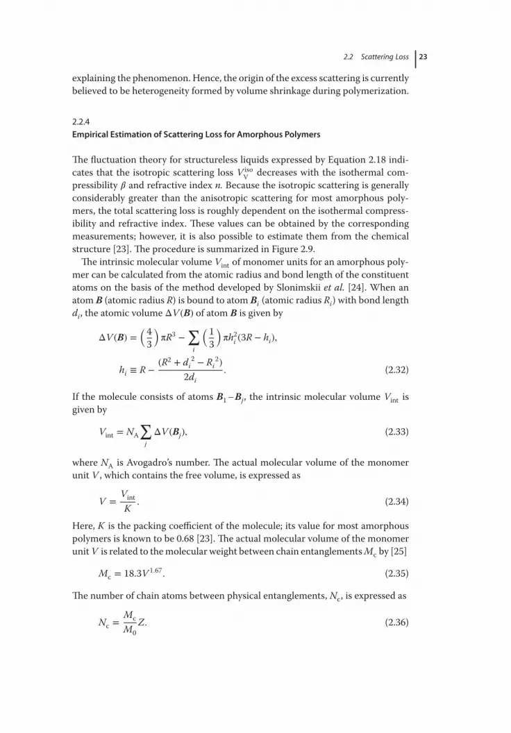
Empirical Estimation of Scattering Loss for Amorphous Polymers

The fluctuation theory for structureless liquids expressed by Equation 2.18 indi-

cates that the isotropic scattering loss V isoV

decreases with the isothermal com-

pressibility 𝛽 and refractive index n. Because the isotropic scattering is generally

considerably greater than the anisotropic scattering for most amorphous poly-

mers, the total scattering loss is roughly dependent on the isothermal compress-

ibility and refractive index. These values can be obtained by the corresponding

measurements; however, it is also possible to estimate them from the chemical

structure [23]. The procedure is summarized in Figure 2.9.

The intrinsic molecular volume Vint of monomer units for an amorphous poly-

mer can be calculated from the atomic radius and bond length of the constituent

atoms on the basis of the method developed by Slonimskii et al. [24]. When an

atom B (atomic radius R) is bound to atom Bi (atomic radius Ri) with bond length

di, the atomic volume ΔV (B) of atom B is given by

ΔV (B) =(4

3

)πR3 −

∑i

(1

3

)πh2

i(3R − hi),

hi ≡ R −(R2 + di

2 − Ri2)

2di. (2.32)

If the molecule consists of atoms B1–Bj, the intrinsic molecular volume Vint is

given by

Vint = NA

∑j

ΔV (Bj), (2.33)

where NA is Avogadro’s number. The actual molecular volume of the monomer

unit V , which contains the free volume, is expressed as

V =Vint

K. (2.34)

Here, K is the packing coefficient of the molecule; its value for most amorphous

polymers is known to be 0.68 [23]. The actual molecular volume of the monomer

unitV is related to themolecular weight between chain entanglementsMc by [25]

Mc = 18.3V 1.67. (2.35)

The number of chain atoms between physical entanglements, Nc, is expressed as

Nc =Mc

M0

Z. (2.36)


Molecular weight betweenchain entanglement

Mc

Intrinsic molecular volumeVint

Actual molecular volumeV

Cross-sectional area per polymer chainA

Isothermal compressibility at Tllβ at Tll

Isothermal compressibility at Tgβ at Tg

Isotropic light scattering intensityVV

iso

Isotropic light scattering lossα iso

Molecular refraction[R ]

Refractive index[n]

Figure 2.9 Flowchart of empirical calculation of isotropic light scattering losses in

amorphous polymers.


Here,M0 is the molecular weight of a monomer unit and Z is the number of chain

atoms in the monomer unit. From the number of chain atoms between physical

entanglements Nc, the cross-sectional area per polymer chain A is obtained as

follows [26]:

logNc = k1 + k2(logA − 2), (2.37)

where k1 and k2 are constants (k1 = 2.929, k2 = 0.614).

Boyer andMiller reported the correlation between the isothermal compressibil-

ity 𝛽 at the liquid–liquid transition temperature T ll and the cross-sectional area

per polymer chain A from the lattice parameters as [27]

log(1011𝛽atTll) = −0.21 + 0.55 logA. (2.38)

The liquid–liquid transition temperature appears to be a useful liquid-state refer-

ence temperature and is usually found by a variety of dynamic and thermodynamic

methods. The concept of T ll was vigorously studied by Boyer. He found that T ll

is near 1.2Tg for most polymers. Lobanov and Frenkel’ [28] estimated T ll for a

variety of polymers from dielectric loss data and proposed an empirical relation

between Tg and T ll:

Tll = Tg + 76 (K). (2.39)

For T ll from 250 to 500K, the numerical difference between the two empirical

rules is small.

By combining the above relationships, the isothermal compressibility 𝛽 of poly-

mers at T ll can be calculated from the intrinsic molecular volume Vint. However,

the value of 𝛽 at Tg is necessary to estimate the light scattering loss in the glassy

state. 𝛽 increases linearly with T from Tg to T ll. It is interesting that the val-

ues of (1∕𝛽at Tll)(d𝛽∕dT) between Tg and T ll for many amorphous polymers are

almost the same (the average value is 4.8× 10−3 K−1) [23]. Considering the value

(1∕𝛽at Tll)(d𝛽∕dT) = 4.8× 10−3 K−1 at Tg <T <Tll and the empirical relationship

between T ll and Tg (T ll =Tg + 76K), we can estimate 𝛽 at Tg from 𝛽 at T ll.

The refractive index of a compound can be calculated from its molar refraction

and molecular volume using the Lorentz–Lorenz equation

n =

√(2[R]V

+ 1

)∕(1 − [R]

V

), (2.40)

where [R] is themolar refraction andV is the actualmolecular volume. [R] is takenas the sum of the atomic refractions.Thus, we can estimate the refractive index of

a polymer from the molar refraction and molecular volume.

Table 2.3 shows the calculated and observed values of the isothermal com-

pressibility, refractive index, and isotropic light scattering of PMMA and PSt.The

calculated values for both polymers show good agreement with the measured

values.


Table 2.3 Isotropic light scattering in PMMA and PSt at 633 nm. Comparison of calculations

from their molecular structures with measurements.

Polymer 𝜷 at Tg (×10−11 cm2/dyn) n V isoV

(×10−6 /cm) 𝜶iso (dB/km)

Calculated Calculated Calculated Observed Calculated Observed

PMMA 3.6 1.494 2.7 2.7 9.8 9.7

PSt 4.4 1.583 5.6 5.9 20.4 21.5

2.3

Low-Loss POFs

2.3.1

PMMA- and PSt-Based POFs

The first POF, Crofon™, which was invented in the mid-1960s by DuPont, was

a multimode fiber with a step-index (SI) profile in the core region. Compared to

GOFs, the SI POF was also advantageous in terms of mass production; it was not

only inexpensive to fabricate but also easy to mold and manufacture. The first

commercial POF was Eska™, a PMMA-based SI POF introduced by Mitsubishi

Rayon in 1975 [29]; subsequently, Asahi Chemical and Toray also entered the

market. However, the first fibers were insufficiently transparent for use as an intra-

building communication medium, and their application was severely limited to

extremely short-range areas such as light guides, illuminations, audio data links,

and sensors.

Through the analyses of each factor in fiber attenuation as described above, the

limitations of POFs based on several materials and their theoretical grounding

have been continually clarified. Further, it has been shown that the major factors

causing high attenuation were not intrinsic but rather extrinsic, such as contam-

inants becoming mixed into the polymer during fiber fabrication. By preparing

the fiber in an all-closed system frommonomer distillation to fiber drawing, low-

loss POFs with losses near the theoretical limits were fabricated. In 1981, Kaino

reported a PSt-based SI POF with an attenuation of 114 dB/km at 670 nm [30],

and in the following year, his group also succeeded in obtaining a PMMA-based

SI POF with an attenuation of 55 dB/km at 568 nm [2].

2.3.2

PMMA-d8-Based POF

Since the first SI POF was commercialized, most POFs have been manufac-

tured using PMMA, a mass-produced, commercially available polymer that

demonstrates high light transmittance and provides excellent corrosion resis-

tance to both chemicals and weather. These properties, coupled with its low

manufacturing costs and easy processing, havemade PMMA a valuable substitute

2.3 Low-Loss POFs 27

for glass in optical fibers. However, the performance can be further improved by

modifying the base material. The high attenuation in conventional PMMA-based

POFs is dominated by C–H overtone stretching and combinations of stretching

and deformation. Hence, the most effective method of obtaining a lower loss

POF is to replace hydrogen with heavier atoms such as fluorine, as shown in

Figure 2.4. However, if vinyl monomers such as MMA are perfluorinated, the

polymerization rate dramatically decreases.

In 1977, DuPont developed an SI POF based on perdeuterated PMMA

(PMMA-d8) [31]. The attenuation spectrum showed low-loss windows at longer

wavelengths such as 690 and 790 nm compared to those of PMMA. This is

because the overtones of molecular vibrational absorption shifted to longer

wavelengths. However, the minimum attenuation of the fiber was still 180 dB/km,

which was even higher than that of PMMA at the time. One of the advantages

of deuteration is that deuterium efficiently reduces the absorption loss at visible

to near-infrared wavelengths but does not affect most other optical and physical

properties because deuterium is an isotope of hydrogen. In other words, the

light scattering intensity of PMMA-d8 should be similar to that of PMMA,

as discussed in Section 2.2.3. Kaino believed that the high attenuation in the

PMMA-d8-based SI POF was caused by extrinsic factors such as scattering losses

due to dust and microvoids and absorption losses due to inorganic contaminants

such as transition-metal ions. Thus, he prepared the fiber using the all-closed

extrusion system that was used to fabricate the low-loss PMMA-based POF

and succeeded in decreasing the attenuation to 20 dB/km at 650–680 nm [32].

In addition, the polymer was extensively studied as a base material for GI

(graded-index) POFs, and an attenuation of 80 dB/km at 650 nm was achieved in

2005 [33].

2.3.3

CYTOP®-Based POF

CYTOP®, developed and trademarked by AGC, is an amorphous perfluorinated

polymer. The first CYTOP-based GI POF, Lucina®, was commercialized in

2001. Figure 2.10 compares the attenuation spectra of PMMA-, PMMA-d8-, and

CYTOP-based GI POFs. CYTOPmolecules consist solely of C–C, C–F, and C–O

bonds. The wavelengths of the fundamental stretching vibrations of these atomic

bonds are relatively long; therefore, the vibrational absorption loss in CYTOP at

the light source wavelengths is negligibly small. In addition, it exhibits fairly low

light scattering because of its low refractive index (nD = 1.34). The attenuation in

a CYTOP-based GI POF is approximately 10 dB/km at 1.0 μm. The theoretical

attenuation spectrum of a CYTOP-based GI POF was calculated using the Morse

potential energy theory and thermally induced fluctuation theory to consider

the inherent absorption and scattering losses, respectively [34]. Given that the

theoretical limit of attenuation is 0.7 dB/km at this wavelength, it is expected

that the attenuation can be lowered further by preventing contamination during

fabrication.


0.1

1

10

100

1000

500 700 900 1100 1300 1500

Attenuation (

dB

/km

)

Wavelength (nm)

CYTOP®

(theoretical values)

CYTOP®

PMMA-d8

PMMA

Figure 2.10 Attenuation spectra of PMMA-, PMMA-d8-, and CYTOP-based GI POFs.

References

1. Urbach, F. (1953) The long-wavelength

edge of photographic sensitivity and of

the electronic absorption of solids. Phys.

Rev., 92 (5), 1324.

2. Kaino, T., Fujiki, M., and Jinguji, K.

(1984) Preparation of plastic optical

fibers. Rev. Electr. Commun. Lab., 32 (3),

478–488.

3. Yamashita, T. and Kamada, K. (1993)

Intrinsic transmission loss of polycarbon-

ate core optical fiber. Jpn. J. Appl. Phys.,

32 (6A), 2681–2686.

4. Atkins, P. and Friedman, R. (2005)

Molecular Quantum Mechanics, Oxford

University Press, New York.

5. Gough, K.M. and Henry, B.R. (1984)

Overtone spectral investigation of

substituent-induced bond-length changes

in gas-phase fluorinated benzenes and

their correlation with ab initio STO-3G

and 4-21G calculations. J. Am. Chem.

Soc., 106 (10), 2781–2787.

6. Henry, B.R. (1987) The local mode model

and overtone spectra: a probe of molec-

ular structure and conformation. Acc.

Chem. Res., 20 (12), 429–435.

7. Snavely, D.L., Blackburn, F.R.,

Ranasinghe, Y., Walters, V.A., and

Gonzalez del Riego, M. (1992) Vibra-

tional overtone spectroscopy of pyrrole

and pyrrolidine. J. Phys. Chem., 96 (9),

3599–3605.

8. Timme, B. and Mecke, R. (1936) Quan-

titative absorptionsmessungen an den

CH-Obserschwingungen einfacher

Kohlenwasserstoffe. Z. Phys., 98 (5),

363–381.

9. Groh, W. (1988) Overtone absorption

in macromolecules for polymer opti-

cal fibers. Makromol. Chem., 189 (12),

2861–2874.

10. Ballato, J., Foulger, S.H., and Smith, D.W.

Jr., (2004) Optical properties of perflu-

orocyclobutyl polymers. II. Theoretical

and experimental attenuation. J. Opt. Soc.

Am. B, 21 (5), 958–967.

11. Koike, K. and Koike, Y. (2009) Design of

low-loss graded-index plastic optical fiber

based on partially fluorinated methacry-

late polymer. J. Lightwave Technol., 27(1), 41–46.

12. Yen, C.-T. and Chen, W.-C. (2003)

Effects of molecular structures on the

near-infrared optical properties of poly-

imide derivatives and their corresponding

optical waveguides. Macromolecules, 36(9), 3315–3319.

13. Ghim, J., Lee, D.-S., Shin, B.G., Vak, D.,

Yi, D.K., Kim, M.-J., Shim, H.-S., Kim,

J.-J., and Kim, D.-Y. (2004) Optical prop-

erties of perfluorocyclobutane aryl ether

References 29

polymers for polymer photonic devices.

Macromolecules, 37 (15), 5724–5731.

14. Takahashi, A., Inoue, A., Sassa, T., and

Koike, Y. (2013) Fluorination effects on

attenuation spectra of plastic optical fiber

core materials. Opt. Mater. Express, 3 (5),

658–663.

15. Olivero, J.J. and Longbothum, R.L.

(1977) Empirical fits to the Voigt line

width: a brief review. J. Quant. Spectrosc.

Radiat. Transfer, 17 (2), 233–236.

16. Liu, Y., Lin, J., Huang, G., Guo, Y., and

Duan, C. (2001) Simple empirical analyt-

ical approximation to the Voigt profile. J.

Opt. Soc. Am. B, 18 (5), 666–672.

17. Einstein, A. (1910) Theorie der

Opaleszenz von homogenen Flüssigkeiten

und Flüssigkeitsgemischen in der Nähe

des kritischen Zustandes. Ann. Phys., 338(16), 1275–1298.

18. Fischer, E.W. and Dettenmaier, M. (1976)

Untersuchungen zu den orientierungs-

und dichtefluktuationen in amorphen

polymeren mit hilfe der lichtstreuung.

Makromol. Chem., 177 (4), 1185–1197.

19. Debye, P. and Bueche, A.M. (1949) Scat-

tering by an inhomogeneous solid. J.

Appl. Phys., 20 (6), 518–525.

20. Hellwege, K.-H., Knappe, W., and

Lehmann, P. (1962) Die isotherme

Kompressibilität einiger amorpher und

teilkristalliner Hochpolymerer im Tem-

peraturbereich von 20–250 ∘C und bei

Drucken bis zu 2000 kp/cm2. Kolloid Z.

Z. Polym., 183 (2), 110–120.

21. Koike, Y., Tanio, N., and Ohtsuka,

Y. (1989) Light scattering and het-

erogeneities in low-loss poly(methyl

methacrylate) glasses. Macromolecules,

22 (3), 1367–1373.

22. Koike, Y., Matsuoka, S., and Bair, H.E.

(1992) Origin of excess light scattering

in poly(methyl methacrylate) glasses.


23. Tanio, N. and Koike, Y. (1997) Estimate

of light scattering loss of amorphous

polymer glass from its molecular struc-

ture. Jpn. J. Appl. Phys., 36 (1–2),

743–748.

24. Slonimskii, G.L., Askadskii, A.A., and

Kitaigorodskii, A.I. (1970) On the

macromolecular packing in polymers.

Vysokomol. Soed., A12 (3), 494–512.

25. Hoffmann, M. (1972) Fließverhalten und

molekulare struktur von polymeren und

ihren lösungen eine systematik quanti-

tativer beziehungen. Makromol. Chem.,

153 (1), 99–124.

26. Boyer, R.F. and Miller, R.L. (1978) Chain

entanglements and chain areas II: a

molecular basis for chain entanglements.

Rubber Chem. Technol., 51 (4), 718–730.

27. Boyer, R.F. and Miller, R.L. (1984) Cor-

relation of liquid-state compressibility

and bulk modulus with cross-sectional

area per polymer chain. Macromolecules,

17 (3), 365–369.

28. Lobanov, A.M. and Frenkel’, S.Y. (1980)

The nature of the so-called “liquid-liquid”

transition in polymer melts. Polym. Sci.

USSR, 22 (5), 1150–1163.

29. Mitsubishi Rayon Co. Ltd. (1975) JP

Patent 1975-83046, filed Nov. 22, 1973

and issued Jul. 4, 1975.

30. Kaino, T., Fujiki, M., and Nara, S. (1981)

Low-loss polystyrene core-optical fibers.

J. Appl. Phys., 52 (12), 7061–7064.

31. Schleinitz, H.M. (1977) Ductile plastic

optical fibers with improved visible and

near infrared transmission. Proceeding

of 26th International Wire and Cable

Symposium, CECOM, Ft. Monmouth, NJ,

November 15–17, pp. 352–355.

32. Kaino, T., Jinguji, K., and Nara, S. (1983)

Low loss poly(methyl methacrylate-d8)

core optical fibers. Appl. Phys. Lett., 42(7), 567–569.

33. Kondo, A., Ishigure, T., and Koike, Y.

(2005) Fabrication process and optical

properties of perdeuterated graded-

index polymer optical fiber. J. Lightwave

Technol., 23 (8), 2443–2448.

34. Tanio, N. and Koike, Y. (2000) What is

the most transparent polymer? Polym. J.,

32 (1), 43–50.

31

3

Transmission Capacity

Thebandwidth of a fiber determines themaximum transmission data rate ormax-

imum transmission distance. Most common POF (plastic optical fiber) transmis-

sion systems adopt on–off keying by directmodulation of the optical source (laser

or light-emitting diode). If an input pulse waveform can be detected without dis-

tortion at the other end of the fiber, themaximum link length is limited by the fiber

attenuation. However, in addition to the optical power attenuation, the output

pulse is generally broader in time than the input pulse.This pulse broadening lim-

its the transmission capacity, namely, the bandwidth of the fiber. The bandwidth

is determined by the impulse response as follows [1]: Optical fibers are usually

considered quasi-linear systems; thus, the output pulse is described by

pout(t) = h(t) ∗ pin(t). (3.1)

The output pulse pout(t) from the fiber can be calculated in the time domain

through the convolution (denoted by *) of the input pulse pin(t) and the impulse

response functionh(t) of the fiber. Fourier transformation of Equation 3.1 provides

a simple expression as the product in the frequency domain:

Pout(f ) = H(f )Pin(f ), (3.2)

whereH(f ) is the power transfer function of the fiber at the baseband frequency f.

The power transfer function defines the bandwidth of the optical fiber as the low-

est frequency at which H(f ) is reduced to half the DC value. The power transfer

function is easily calculated from the Fourier transform of the experimentally

measured input and output pulses in the time domain, or from the measured out-

put power from the fiber in the frequency domain from DC to the bandwidth

frequency. A higher bandwidth yields less pulse broadening and enables higher

speed data transmission. The bandwidth limitation also largely determines the

maximum link length for a given data rate in some multimode fiber (MMF) sys-

tems. Pulse broadening, which is theoretically proportional to the fiber length in

the absence of mode coupling, is caused mainly by two dispersion mechanisms

in POFs: intermodal and intramodal dispersion. The root mean squared (rms)

width of the impulse response 𝜎 is calculated by 𝜎 =√

𝜎2inter

+ 𝜎2intra

, where 𝜎inter

and 𝜎intra are the rms widths of the pulse broadening induced by intermodal and

intramodal dispersion, respectively. Another type of dispersion, called polariza-

tion mode dispersion, arises from the anisotropies of the structure and material,


32 3 Transmission Capacity

which results in slightly different propagation constants for the two orthogonal

polarization modes [2]. The effect of polarization mode dispersion can usually be

ignored inMMFs.Therefore, this chapter explains the intermodal and intramodal

dispersion and the bandwidths of POFs.

3.1

Bandwidth

3.1.1

Intermodal Dispersion

When an optical pulse is input into an MMF, the optical power of the pulse

is generally distributed into the huge number of modes of the fiber. Different

modes travel at different propagation speeds along the fiber; thus, different modes

launched at the same time reach the output end of the fiber at different times.

Therefore, the input pulse is broadened in time as it travels along the MMF. This

pulse broadening effect, well known asmodal dispersion, is significantly observed

in step-index (SI) MMFs. Different rays travel along paths with different lengths,

where each distinct ray can be thought of as a mode in a simple interpretation.

The light travels at the same velocity along its optical path because of the constant

refractive index throughout the core region in SI MMFs. Consequently, the same

velocity but different path lengths result in different propagation speeds along the

fiber, which causes a pulse spread in time.The pulse broadening caused by modal

dispersion seriously limits the transmission speed in MMFs because overlapping

of the broadened pulses induces intersymbol interference and disrupts correct

signal detection, thereby increasing the bit error rate [3].

Modal dispersion is generally a dominant factor in pulse broadening in MMFs,

and in particular in SI MMFs. As shown in [4] for an ideal SI MMF, the difference

in the propagation delay between the fastest and slowest modes is given by

Δtmod =L

2cn2NA2, (3.3)

where L is the fiber length, n1 and n2 are the core and cladding refraction

indices, respectively, and NA = numerical aperture =√

n21− n2

2. For instance,

for a typical NA of 0.5, after 50m of SI POF, one would obtain a Δtmod of

14.8 ns, and thus an estimated electrical-to-electrical available bandwidth of

B ≅ 0.44∕Δtmod ≈ 30MHz under worst case conditions. The actual bandwidth

depends on several other parameters, related mainly to the NA of the source,

the level of mode mixing inside the POF, and the fact that higher order modes

(which travel more slowly) usually see higher attenuation and thus contribute

less to the overall transfer function (see again [4]) than lower order modes. As a

result, the actual available bandwidths for SI POFs are higher than those given by

the theoretical treatment above, but are still limited to less than approximately

100MHz over 50m.

3.1 Bandwidth 33

However, the modal dispersion can be dramatically reduced by forming a

near-parabolic refractive index profile in the core region of the MMF, which

allows a much higher bandwidth (i.e., higher-speed data transmission) [5]. A

typical graded-index (GI) MMF has a cylindrically symmetric refractive index

profile that gradually decreases from the core axis to the core–cladding interface.

A ray confined near the core axis, corresponding to a lower order mode, travels a

shorter geometrical length at a slower light velocity along the path because of the

higher refractive index. A sinusoidal ray passing through near the core–cladding

boundary, considered as a higher order mode, travels a longer geometrical length

at a faster velocity along the path, particularly in the lower refractive index region

far from the core axis. As a result, the output times from the fiber end of light

traveling the shorter geometrical length at the slower velocity and the longer

geometrical length at the faster velocity can bemade almost the same by using the

optimum refractive index profile. Thus, the refractive index distribution strongly

affects the bandwidth of MMFs. The optimization of the refractive index profile

in GI MMFs is an important issue in reducing the modal dispersion. A power-law

index profile approximation is a well-known method of analyzing the optimum

profile of GI MMFs [6]. In this approximation, the refractive index distribution of

a GI MMF is described by

n(R) =⎧⎪⎨⎪⎩n1

[1 − 2Δ

(R

a

)g] 1

2

for 0 ≤ R ≤ a

n2 for R > a

, (3.4)

where n(R) is the refractive index as a function of the radial distance R from the

core center, n1 and n2 are the refractive indices of the core center and the cladding,

respectively, and a is the core radius.The profile exponent g determines the shape

of the refractive index profile, and Δ is the relative index difference, given by

Δ =n21− n2

2

2n21

. (3.5)

Equation 3.4 includes the SI profile when g =∞.

The optimum profile exponent gopt, which minimizes the modal dispersion

and the difference in the delay of all the modes and maximizes the bandwidth, is

expressed as follows on the basis of an analysis of scalar wave equation:

gopt = 2 + 𝜂 − Δ(4 + 𝜂)(3 + 𝜂)5 + 2𝜂

, (3.6)

𝜂 = −2n1N1

𝜆

ΔdΔd𝜆

, N1 = n1 − 𝜆dn1d𝜆

(3.7)

If the refractive index of the material is wavelength-independent, Equation 3.6

becomes the simple expression

gopt = 2 − 12

5Δ. (3.8)


Ahigh bandwidth can typically be achievedwhen the profile exponent g is approx-

imately equal to 2.0. However, the refractive indices of materials generally depend

on the wavelength, which induces profile dispersion.

The profile dispersion p caused by the wavelength dependence of the refractive

index [7] is given by

p = 𝜆

ΔdΔd𝜆

. (3.9)

The gopt value depends on the relative index difference Δ, which is a function of

the refractive indices of the core and the cladding. These refractive indices are

determined by the wavelength and the dopant characteristics. If the refractive

indices of the polymermatrix and dopant have identical wavelength dependences,

gopt obeys Equation 3.8. However, the wavelength dependence of the refractive

index of the dopant generally differs from that of the polymer matrix; hence, the

shape of the refractive index profile depends on the wavelength.Therefore, even if

the optimum refractive index profile is provided at a certain wavelength, this pro-

file differs from the optimumprofile at another wavelength. Profile dispersion also

depends on the wavelength of the light signal. The effect of profile dispersion can

be compensated in the refractive index profile by taking it into account, which is

easily illustrated by Equations 3.6, 3.7, and 3.9. Thus, the gopt value is shifted by

profile dispersion. Consequently, the intermodal dispersion can be minimized by

using the optimum refractive index profile considering profile dispersion. Then,

intramodal dispersion becomes important for achieving high bandwidth. Addi-

tionally, single-mode fibers (SMFs) exhibit even higher bandwidths thanGIMMFs

because modal dispersion does not exist in principle; thus, intramodal dispersion

seriously limits the bandwidth of SMFs [8].

3.1.2

Intramodal Dispersion

Intramodal dispersion or chromatic dispersion is the pulse widening caused by the

finite spectral width of the light source. Intramodal dispersion comprises mate-

rial and waveguide dispersion. Material dispersion is induced by the wavelength

dependence of the refractive index of the core material [9]. The group velocity of

a given mode depends on the wavelength; thus, the output pulse is broadened in

time even when optical signals with different wavelengths follow the same path.

This effect is generally much smaller than modal dispersion in MMFs but is no

longer negligible when the modal dispersion is sufficiently suppressed.

Waveguide dispersion arises from the wavelength dependence of the optical

power distribution of a mode between the core and the cladding. Light at shorter

wavelengths is more completely confined to the core region, and light at longer

wavelengths is distributed more in the cladding. Because more longer wavelength

light is in the cladding, it travels at a higher propagation speed, as the refractive

index of the cladding is lower than that of the core.

3.1 Bandwidth 35

100-m multi SI POF230 MHz

50-m SI POF240 MHz

100-m GI POF2.65 GHz

2 ns/div

Input pulse

Figure 3.1 Measured output pulse waveforms through 50-m SI POF, 100-m multi-SI POF,

and 100-m GI POF under overfilled launch condition.

3.1.3

High-Bandwidth POF

A large number of modes, typically more than tens of thousands, can propagate

in POFs because of the large cores. Therefore, reducing modal dispersion has

been a key issue in such multimode POFs.Themeasured output pulse waveforms

frompoly(methylmethacrylate)- (PMMA-) based SI,multi-SI, andGI POFs under

overfilled launch conditions are shown in Figure 3.1 in comparison with the input

pulse waveform.The bandwidth of the SI POF was seriously limited. The impulse

responses and bandwidths of the SI andmulti-SI POFs were almost the same, even

though the multi-SI POF was twice as long as the SI POF. The multi-SI POF can

realize communication at a data rate twice as high as that of the SI POF; how-

ever, the bandwidth was still limited to hundreds of megahertz for 100m. The GI

POF was proposed to reduce the bandwidth limitation caused by the large modal

dispersion of the SI POF [10], and the refractive index profile can be precisely con-

trolled and optimized. The bandwidth of the GI POF was dramatically enhanced

to several gigahertz over 100m by such control of the index profile. This is due

to the decrease in modal dispersion caused mainly by the graded refractive index

profile. Thus, the GI POF is a promising candidate for a transmission medium for

high-speed and short-reach networks.

Figure 3.2 shows the effects of individual types of dispersion on the bandwidth

characteristics of PMMA-based GI POFs. Here, the bandwidths were estimated

by the Equations 3.10–3.12 [11, 12]. Gaussian pulses were assumed, and the rms

spectral width was set to 1 nm.


10.1

1

10

100

3 5

Measured

All types of dispersions were considered

Modal and profile dispersions were considered

Modal dispersion was considered

Profile exponent g

Ba

nd

wid

th f

or

10

0 m

(G

Hz)

7

Figure 3.2 Calculated bandwidth of 100-

m PMMA-based GI POF as a function of

the profile exponent g at a wavelength

of 650 nm considering individual types of

dispersion compared with the measured

bandwidths under overfilled launch condi-

tions. An rms spectral width of 1 nm was

assumed.

𝜎inter =LN1Δ2c

g

g + 1

(g + 2

3g + 2

) 1

2

[C21 +

4C1C2Δ(g + 1

)2g + 1

+4Δ2C2

2(2g + 2)2

(5g + 2)(3g + 2)

] 1

2

,

(3.10)

𝜎intra =L𝜎𝜆c𝜆

⎡⎢⎢⎣(−𝜆2n′′

1

)2 − 2𝜆2n′′1(N1Δ)

(g−2−𝜂g+2

)(2g

2g+2

)+(N1Δ)2

(g−2−𝜂g+2

)24g2

(g+2)(3g+2)

⎤⎥⎥⎦ , (3.11)

C1 =g − 2 − 𝜂

g + 2, C2 =

3g − 2 − 2𝜂

2(g + 2

) . (3.12)

The maximum bandwidth, ∼100GHz for 100m, was theoretically obtained

when g was almost 2.0 if only the modal dispersion was considered. How-

ever, large discrepancies were observed between the calculated and measured

bandwidths. In contrast, the relation between the bandwidth and the pro-

file exponent of PMMA-based GI POFs was accurately estimated by the

Wentzel–Kramers–Brillouin method when all the dispersion factors were taken

into account.

On the other hand, the gopt value, which represents the highest bandwidth,

shifted to around 2.4 because of profile dispersion, as discussed above.The dopant

used in all the GI POFs shown in Figure 3.2 was diphenyl sulfide, and all the GI

POFs had NAs of ∼0.20. This result indicates that the bandwidth characteristics

are strongly influenced by the profile dispersion even if the refractive index profile

deviates greatly from the ideal one.

3.1 Bandwidth 37

500−0.8

−0.6

−0.4

−0.2

0

0.2

700 900

CYTOP

Silica

PMMA

1100

Wavelength (nm)

Ma

teria

l d

isp

ers

ion

(p

s/(

nm

·km

))

1300 1500

Figure 3.3 Material dispersion of PMMA, CYTOP, and silica.

The calculated maximum bandwidth at gopt was dramatically reduced owing to

the large material dispersion of PMMA when all types of dispersion were consid-

ered. A significant decrease in bandwidth was observed mainly for profile expo-

nents near the gopt value. When the profile exponent deviates greatly from gopt,

material dispersion has little effect on the bandwidth because of the dominant

large modal dispersion.

The bandwidth of the PMMA-based GI POFs can be optimized by accurate

control of the refractive index profile [13]. Further bandwidth improvement has

been investigated by using perfluorinated (PF) polymers [14]. PF polymers have

the valuable characteristics of lowmaterial dispersion and low transmission losses

(see Chapter 2). Figure 3.3 shows the material dispersion in PMMA (a PF polymer

commercially available fromAsahi Glass Co.), and silica calculated from thewave-

length dependence of their refractive indices.Thematerial dispersion of CYTOP®is much smaller than that of PMMA and even that of silica, particularly in the vis-

ible to near-infrared region, which means that CYTOP-based GI POFs with an

optimum refractive index profile can realize higher bandwidths than silica-based

GI MMFs. The material dispersion curve of CYTOP was insensitive to the wave-

length, unlike those of silica and PMMA. Hence, the bandwidth of CYTOP-based

GI POFs is also expected to be insensitive to the wavelength.Thus, CYTOP-based

GI POFs are predicted to have a higher bandwidth than silica-based GI MMFs.

The PF GI POFs, indeed, demonstrated data transmission rates of 40Gb/s and

even higher over 100m [15–17].

The wavelength dependence of the bandwidths of 100-m PMMA- and CYTOP-

based GI POFs and a silica-based GI MMF was theoretically estimated from

the wavelength dependence of their refractive indices, as shown in Figure 3.4.

The refractive index profiles of all the fibers were optimized at a wavelength of

850 nm, and the rms spectral width of the light source was assumed to be 1.0 nm.

The bandwidth at 850 nm of the PMMA-based GI POF, almost 10GHz, was

higher than that at 650 nm because of the lower material dispersion, although

a light signal at 850 nm cannot travel a long distance in PMMA because of the


5001

10

100

700 900 1100

Wavelength (nm)

Bandw

idth

for

100 m

(G

Hz)

1300

CYTOP

SilicaPMMA

1500

Figure 3.4 Calculated bandwidths of PMMA- and CYTOP-based GI POFs and silica-based GI

MMF as a function of wavelength. Refractive index profiles were optimized at a wavelength

of 850 nm, and the rms spectral width of light source was assumed to be 1 nm.

large transmission loss. The wavelength dependence of the optimum profile of

the CYTOP-based GI POF was small, as mentioned above, because CYTOP

has low material and profile dispersions. Therefore, the CYTOP-based GI POF

can maintain its high-bandwidth characteristics over a wide wavelength range

compared to silica-based GI MMFs. Consequently, CYTOP-based GI POFs

can use various light sources with a larger variety of wavelengths; hence, more

channels are available in wavelength division multiplexing systems.This indicates

that CYTOP-based GI POFs can realize higher data rate transmission systems.

3.2

Wave Propagation in POFs

The transmission bandwidths of GI POFs have been extended with the develop-

ment of low-dispersivematerials andGI profile control techniques. Consequently,

a 40-Gbps serial transmission over 100m of GI POFs has been demonstrated. It

has also been reported that the transmission characteristics of GI POFs are signifi-

cantly affected bymuch strongermode coupling than that in glassMMFs [18–20],

although the underlying physics is not well understood. This suggests that mode

coupling in GI POFs can originate in some phenomenon other than microbend-

ing, the predominant origin in glassMMFs, whose mode coupling effects can typ-

ically be observed for transmission over several kilometers [6]. Therefore, mode

coupling in GI POFs cannot be analyzed using the conventional diffusion theory

of coupled power equations [21].

Optical fiber materials exhibit density fluctuations because of their amorphous

nature. These fluctuations in glasses result in Rayleigh scattering because their

characteristic scales are much smaller than the wavelengths of guided light used

in glass MMFs. Rayleigh scattering induces randommode coupling, but the effect


is tooweak to influence the transmission bandwidth of glassMMFswith lengths of

less than several hundred meters. However, polymers such as PMMA have longer

scale fluctuations of microscopic heterogeneous structures [22, 23]. Therefore,

microscopic heterogeneities in POF cores can result inmode coupling because the

POF cores exhibit greater forward scattering than glasses. However, the intrinsic

material properties have been overlooked in the transmission analyses of GI POFs.

Here, we clarify the effect of the intrinsic microscopic properties on the macro-

scopically observed transmission characteristics of GI POFs. Moreover, we show

that intrinsic mode coupling results in significant noise reduction inMMF optical

links, which allows low-cost radio-over-fiber (RoF) systems in home and building

networks.

3.2.1

Microscopic Heterogeneities

As mentioned in Chapter 2, attenuation in GI POFs has been sufficiently reduced

for short-reach applications, according to our study of light scattering in GI

POF core bulk polymers. However, the remaining scattering losses in GI POFs

are much higher than those in glass MMFs. Actually, we can visually observe

streaking of the light trajectory in a PMMA-based GI preform because of the

intrinsic forward scattering, as shown in Figure 3.5. This indicates that GI POF

cores can have microscopic heterogeneities in their higher order structures,

which can result in stronger mode coupling because greater forward scattering

occurs than in glass MMFs.

Themicroscopic heterogeneities in actualGI POF cores can be influenced by the

fabrication processes, and their correlation characteristics differ significantly from

those of the polymer bulk. In GI POFs, moreover, guided light waves can interact

withmicroscopic heterogeneities through fluctuations in the cross-sectional com-

ponents of the dielectric constants along the fiber axis because the guided wave

fronts are almost parallel to the cross section in GI POFs under the weakly guid-

ing approximation. This makes the experimental evaluation of the microscopic

Figure 3.5 Visually observable light trajectory due to forward scattering by microscopic

heterogeneous structures in PMMA-based GI preform.


heterogeneities in GI POF cores difficult. Therefore, light scattering by micro-

scopic heterogeneities in actual GI POF cores has not been well understood.

3.2.2

Debye’s Scattering Theory

Light scattering by microscopic heterogeneities can be understood in terms of

the Rayleigh–Debye scattering theory [24], which Debye et al. [25, 26] applied

to problems regarding the characterization of inhomogeneities in solids by light

or X-ray scattering measurements. According to their methods, the light scatter-

ing intensity pattern can be related to the spatial correlation characteristics of the

dielectric constant fluctuations, which reflect the microscopic material proper-

ties. Here, the light scattering theory is briefly summarized to understand light

scattering by microscopic heterogeneities in polymers.

Let us consider monochromatic light scattered from an inhomogeneous solid

with an average dielectric constant 𝜀av on which are superimposed local fluctua-

tions 𝛿𝜀. For a weakly scatteringmedium, where the fluctuation is small compared

to the average, the single-scattering approximation can be applied to a scattered

light field because the incident light is perturbed little by the fluctuation [24, 27]. In

the Rayleigh–Debye approximation, the scattered field amplitude in the far zone

can be expressed as a superposition of contributions from volume elements:

F(s) = ∫ 𝛿𝜀(r)e−iks⋅rdr, (3.13)

with

s = S − S0. (3.14)

Here, S and S0 are the unit wave vectors of scattered and incident light, respec-

tively, and k is the light wavenumber 2𝜋/𝜆, where 𝜆 is the wavelength. The ampli-

tude of F(s) without the proportionality factor is analogous to the form factor of an

atom in X-ray scattering. A photodetector measures not the scattered light ampli-

tude but the scattered light intensity, which is proportional to a time average of the|F(s)|2 value. For amorphous materials, the dielectric constant fluctuations can be

considered to be density fluctuations that are frozen in at the glass transition tem-

perature. Assuming that the dynamic fluctuation is a stationary ergodic process,

the scattering light intensity can be expressed as

I(s) = ⟨|F(s)|2⟩ = V∫ 𝛾(r)eiks⋅rdr, (3.15)

where the angle brackets represent the ensemble average. V is the irradiated vol-

ume and 𝛾(r) is the autocorrelation function, which is defined as the ensemble-

averaged product of the fluctuation 𝛿𝜀1 and 𝛿𝜀2 at two points with a separation

distance of r. In the derivation of Equation 3.15, we assumed an isotropic fluctua-

tionwhose autocorrelation function depends only on the distance r.Therefore, the

following expression is also obtained by performing the integral in Equation 3.15

over all directions:


Angular dependence I(s)of scattering intensity

Correlation function γ(r)of dielectric constant fluctuation

Laser

Fourie

r transfo

rmHigher dielectric constantLower dielectric constant

Figure 3.6 Light scattering by microscopic heterogeneities.

I(s) = V∫∞

0

4𝜋r2𝛾(r) sin(ksr)ksr

dr, (3.16)

where s= |s|. Equation 3.15 shows that the scattering intensity pattern of the poly-mers is related to the autocorrelation function of microscopic heterogeneities by

the Fourier transform, as shown in Figure 3.6. Assuming Gaussian-correlated het-

erogeneities, the autocorrelation function is given by

𝛾(r) = ⟨𝛿𝜀2⟩ exp(− r2

D2

), (3.17)

where the correlation length D and mean square fluctuation ⟨𝛿𝜀2⟩ correspond to

measures of the fluctuation size and amplitude, respectively. The fluctuation size

or correlation length determines the angular scattering profile, and the fluctua-

tion amplitude controls the scattering efficiency. From Equations 3.15 and 3.17,

we obtain the intensity of light scattered from the microscopic heterogeneities,

as

I(s) = V ⟨𝛿𝜀2⟩4𝜋 3

2D3e−k2s2D2

4

4 + k2s2D2. (3.18)

A longer correlation length results in more forward scattering, as shown in

Equation 3.18. Microscopic heterogeneities have a larger scale correlation of

the dielectric constant fluctuation than those in optical glasses. Therefore, the

optical transmission characteristics of POFs differ inherently from those of glass

MMFs through random mode coupling due to greater forward scattering by the

microscopic heterogeneities.


3.2.3

Developed Coupled Power Theory

Microscopic heterogeneities in POF core materials result in random power tran-

sitions between the guided modes through forward scattering, as illustrated in

Figure 3.7. Mode coupling can affect the mode power distribution and thus the

transmission bandwidth [28]. Power transitions from guided modes to radiation

modes are also induced; this is one of the main mechanisms for the much higher

losses in POFs than in glass MMFs. However, the radiation mode coupling has lit-

tle effect on the transmission bandwidth because the radiation loss due to volume

scattering by the heterogeneities has no strong mode dependence. In this section,

we revisit and develop a coupled power theory for understanding the intrinsic

guided mode coupling in POFs.

The transverse electric fields in heterogeneous POFs can be approximately

expressed as a superposition of the transverse guided mode fields of the ideal

optical fiber without any inhomogeneities:

E(x, y, z) =N∑i=1

ci(z)Ei(x, y) exp(i𝛽iz), (3.19)

where Ei and 𝛽 i are the transverse electric field vector and the propagation

constant for mode i of the ideal optical fiber with N modes, respectively. In

Equation 3.19, we ignore the contributions of the backward-propagating modes

and radiation modes. For the guided mode fields, the following orthogonality

condition is satisfied:

1√2∫

∞

−∞ ∫∞

−∞ez ⋅ (Ej ×H i

∗)dxdy = 𝛿jiP, (3.20)

Dielectric constantfluctuations

z

x

y

Mode j

Mode i

Polymer chains

HeterogeneousPOF core

Figure 3.7 Random mode coupling due to microscopic heterogeneities.


where ez is the unit vector along the fiber axis and P is the normalized coefficient.

In a heterogeneous POF, the transverse electric field or the expansion coefficients

of the guided light waves change with propagation by mode coupling of the het-

erogeneities, obeying the coupled mode equation

∂ci∂z

=∑j

Kijcj exp[i(𝛽i − 𝛽j)z] (3.21)

with

Kij =𝜔

4iP∫∞

−∞ ∫∞

−∞𝛿𝜀(x, y, z)(Ei

∗ ⋅ Ej)dxdy. (3.22)

Here, 𝜔 is the angular frequency of the guided light, and Kij is the mode coupling

coefficient. In the derivation of Equation 3.22, the contribution of the longitudinal

field components is ignored in the weakly guiding approximation. As shown by

Equation 3.22, the mode coupling coefficient depends on the exact distribution

of the dielectric constant fluctuation. For random fluctuations of the microscopic

heterogeneities, the ensemble-averaged power can be analyzed using the coupled

power equation [28]

∂Pi∂z

+ 𝜏i∂Pi

∂t= −𝛼iPi +

N∑j=1

hij(Pj − Pi), (3.23)

where hij is the power coupling coefficient from mode j to mode i, 𝜏 i is the group

delay per unit length for mode i, and 𝛼i is the attenuation coefficient for mode i.

Pi(j) is the ensemble-averaged mode power <|ci|2> over slightly different optical

fibers with statistically similar perturbations. In the original derivation of the cou-

pled power equation, directional perturbations along the optical fiber axis (z-axis)

are assumed because the fiber axis fluctuation and core diameter fluctuation can

be the dominant sources of mode coupling in glass MMFs. On the other hand, the

microscopic heterogeneities in POF cores are basically isotropic perturbations.

Therefore, we use the generalized power coupling coefficients to take account of

the perturbation isotropy [29]:

hij = ∫∞

−∞⟨Kij(z)K∗

ij(z + 𝜁)⟩ exp[𝑖𝛥𝛽𝜁 ]d𝜁, (3.24)

where Δ𝛽 (= 𝛽 i − 𝛽 j) is the propagation constant difference. From Equations 3.17

and 3.24, we obtain the following power coupling coefficient for microscopic het-

erogeneities in POF core materials [30]:

hij = Cij∫ ∫ |E∗i ⋅ Ej|2dxdy, (3.25)

where

Cij = ⟨𝛿𝜀2⟩𝜔2𝜋3

2D3

8P2exp

(−Δ𝛽2D2

4

). (3.26)

The range of the integral on the right-hand side in Equation 3.25 is the core region.

In the derivation of Equation 3.25, we assumed a shorter correlation length than


the characteristic scale of the mode field variation, allowing the approximation

of the Gaussian correlation function in the fiber cross section by the delta func-

tion product [31]. As shown in Equation 3.25, the power coupling coefficients

are determined by the scattering characteristics of the materials and the field

intensity overlap of the modes, which are given by Cij and ∫∫ |Ei*⋅Ej|2dxdy,

respectively. Note that the coupling coefficient depends little on the propagation

constant difference because exp(−Δ𝛽2D2/4)≈ 1 for the typical correlation length

of the microscopic heterogeneities. This indicates that the mode coupling due

to the heterogeneities should not be a diffusion process like the microbending-

induced coupling, which occurs between nearest neighbor modes with the closest

propagation constants.

3.2.4

Mode Coupling Mechanism

Using the developed coupled power theory, we can evaluate random mode cou-

pling due to microscopic heterogeneities in PMMA-based GI POFs. Here, we

analyze the parabolic refractive index profile whose guided modes can be classi-

fied into principal mode groups with almost the same group velocity, which helps

in understanding the optical pulse transmission of the GI POF.The index profile is

given by Equation 3.4, where g = 2 and a= 25 μm. For typical PMMA cores doped

with diphenyl sulfide, n1 = 1.503 and n2 = 1.490 for a laser source wavelength of

650 nm [32]. To calculate the power coupling coefficients using Equations 3.25

and 3.26, the propagation constants, mode fields, and group delays of the GI POF

were calculated using finite element analysis of the scalar wave equation for the

linearly polarized LPm,l modes, where m is the azimuthal mode number and l is

the radial mode number. The GI POF has 147 LP modes, which can be classified

into 24 principal mode groups. The highest order mode group was ignored in the

analyses of the impulse response because the modes in the group can easily radi-

ate from the fiber owing to their much lower power confinement in the core than

other groups.

Figure 3.8 shows Cij as a function of the correlation length for ⟨𝛿𝜀2r ⟩ =2.0 × 10−8, where 𝛿𝜀r is the relative dielectric constant fluctuation. For guided

mode coupling (closed circles), Cij increases approximately with the cube of

the correlation length, as mentioned in the previous subsection. The increase is

attributed to the scattering profile change from isotropic scattering to forward

scattering, which has more small-angle components corresponding to differences

in the guided mode propagation constant. For the radiative mode coupling

(dotted lines), the Cij value depends strongly on the |Δ𝛽| value, and the |Δ𝛽|dependence is stronger for a longer correlation length. Figure 3.8 shows that the

Cij value decreases with an increase in the |Δ𝛽| value or scattering angle. This

indicates that a longer correlation length results in more forward scattering with

fewer wide-angle components. Note also that all guided mode pairs have almost

the same Cij values. This indicates that the correlation lengths have little effect

on the power transition pathway, which is determined by the mode dependence


00.01

Cij

(a.u

.)

0.1

1

10

~ 0

0.12

14.5

5

10

|Δβ | (μm−1)

100

100 200 300

Correlation length D (nm)

Figure 3.8 Coefficient Cij as a function of

correlation length D for several |Δ𝛽| values,including the minimum and maximum values

for guided mode pairs. Insets schematically

show scattering vectors (black solid arrows)

with propagation vectors of scattered (gray

solid arrows) and incident (gray dotted

arrows) light along the z-axis.

0

1

0

2

5

3

hij

(10

−4 m

−1)

4

1 2 3 4 5

∫∫ ⎜Ei ∗ · Ej ⎜2 dxdy (a.u.)

Figure 3.9 Power coupling coefficient as a function of ∫∫ |Ei*⋅Ej|2dxdy.of the coupling coefficient. Figure 3.9 shows the power coupling coefficient

as a function of ∫∫ |Ei*⋅Ej|2dxdy for D= 300 nm. The coupling coefficient is

approximately proportional to ∫∫ |Ei*⋅Ej|2dxdy because all the guided mode pairs

have almost the same Cij values. This indicates that the power transition pathway

is predominantly determined by the mode field intensity overlaps, which depend

on the structural parameters of the GI POFs.

As the parabolic index profile is not optimum for PMMA-based GI POFs, ran-

dom mode couplings can affect pulse spreading owing to group delay averaging.


Correlation length D (nm)

0.5

0.9

0.8

<δεr

2> = 0.5 × 10

−8

<δεr

2> = 1.0 × 10

−8

<δεr

2> = 2.0 ×

10−8

0.7

0.6

1.0

−3 d

B b

andw

idth

(G

Hz)

0 100 200 300

Figure 3.10 −3 dB bandwidth of 200-m GI POF as a function of correlation length for sev-

eral ⟨𝛿𝜀2r ⟩ values.Using the power coupling coefficient hij and the modal delay per unit length 𝜏 i,

we investigate the optical pulse response of a GI POF at a wavelength of 650 nm

in an overfilled launch condition with a homogeneous mode power distribution

for all x-polarized LP modes using the numerical analysis of Equation 3.23 con-

sidering LP mode degeneracy. Here, only the x-polarized LP mode couplings are

evaluated, assuming that the optical source is linearly polarized and that the GI

POF has no structural or material anisotropies. In addition, the attenuation is not

taken into account in the numerical calculation because it has no significant effect

on the pulse response in the absence of mode-dependent attenuation. Actually,

the radiative mode coupling or scattering loss due tomicroscopic heterogeneities,

which is the origin of the attenuation, has no strong dependence on the mode

number. Figure 3.10 shows the −3 dB bandwidth of a 200-m GI POF as a func-

tion of the correlation length for several ⟨𝛿𝜀2r ⟩ values. The results show that the

bandwidth can increase with the size and/or amplitude of the density fluctuations

in the core polymers. This should be attributed to group delay averaging through

random power transitions [28], whose transition rates are equally enhanced for all

the mode pairs through changes in the scattering directions and/or efficiencies,

as shown in Equations 3.25 and 3.26. This suggests that the optical fiber band-

widths can depend on the macroscopically observed GI profiles as well as on the

microscopic material properties.

3.2.5

Efficient Group Delay Averaging

To further understand the intrinsic mode coupling, we investigated the optical

pulse response of GI POFs in detail [33]. Figure 3.11a shows the power coupling

coefficients for intrinsic mode coupling due to microscopic heterogeneities with


010−5

10−4

10−3

10−2

0.05 0.10

Δβ (μm−1)

hij

(μm

−1)

10−5

10−4

10−3

10−2

hij

(μm

−1)

0.15 0 0.05 0.10

Δβ (μm−1)

0.15

(a) (b)

Figure 3.11 Power coupling coefficients hij as a function of propagation constant differ-

ence Δ𝛽 for mode coupling due to (a) microscopic heterogeneities and (b) microbending.

D= 300 nm and ⟨𝛿𝜀2r ⟩ = 2.0 × 10−8 as a function of the propagation constant dif-

ference of the coupled mode pair. It was confirmed that the Δ𝛽 values can be

approximately classified into 24 discrete values corresponding to all the mode

group pairs because of the parabolic index profile. Therefore, the result indicates

that microscopic heterogeneities can induce random power transitions between

all the group pairs. As shown in Figure 3.11b, we also calculated the coupling

coefficient for microbending-induced coupling assuming that the bending curva-

ture is Gaussian-correlated [34]. The standard deviation and correlation length

of the curvature are 2× 10−4/mm and 1.0mm, respectively, which are close to

the reported values for glass MMFs. Microbending causes only coupling between

the nearest neighbor groups, obeying the selection rules for mode coupling [21].

Note that the average coupling coefficient of 4.1× 10−5/m for microscopic hetero-

geneities is much smaller than the coefficient of 8.4× 10−4/m for microbending.

For the parabolic refractive index profiles, the optical pulse response of GI POFs

can be understood by considering mode couplings between the principal mode

groups. Figure 3.12a,b shows the average coupling coefficientHMN betweenmode

groups with the principal mode numbersM andN calculated formicroscopic het-

erogeneities andmicrobending, respectively.Note thatH11 andH22 have no values

because mode groups 1 and 2 have only one guided mode each. The results show

that forward scattering by microscopic heterogeneities can contribute to both

intragroup (M=N) and intergroup (M≠N) mode couplings, whereas only near-

est neighbor couplings can be induced by microbending. Note also that intrinsic

mode coupling due to microscopic heterogeneities is stronger for lower order

mode groups owing to higher degrees of mode field intensity overlap. However,

the coupling coefficients for microbending-induced coupling become larger for

higher order group pairs, as shown in Figure 3.12b.

Figure 3.13a–c shows the output pulse waveform from GI POFs with micro-

scopic heterogeneities, with microbending, and without any perturbations, cal-

culated for different fiber lengths. The temporal pulse shape of the incident light

is Gaussian with a full width at half-maximum of 83 ps. Owing to intermodal

48 3 Transmission CapacityP

rincip

al m

ode n

um

ber

M

10 201

Principal mode number N

10 201

Principal mode number N

1

10

20

Princip

al m

ode n

um

ber

M

1

10

20

10−3

10−4

10−5

10−3

10−4

10−5

(a) (b)

Figure 3.12 Average power coupling coefficients between mode groups with principal

mode numbers M and N for random mode coupling due to (a) microscopic heterogeneities

and (b) microbending.

Relative delay (ns) Frequency (GHz)

0

(a)

(b)

(c) (f)

(e)

(d)

1 2 0 2 41 3 5

Fre

qu

en

cy

resp

on

se

(d

B)

Po

we

r (a

.u.)

0

1

−30

−20

−10

Fre

qu

en

cy

resp

on

se

(d

B)

−30

−20

−10

0

Fre

qu

en

cy

resp

on

se

(d

B)

−30

−20

−10

0

0

Relative delay (ns)

0 1 2

Frequency (GHz)

0 2 41 3 5

Po

we

r (a

.u.)

0

1

Relative delay (ns)

0 1 2

Frequency (GHz)

0 2 41 3 5

Po

we

r (a

.u.)

0

1

With microbendingWith heterogeneity

With out perturbation

100 m

200 m

50 m

100 m

200 m

Figure 3.13 Output pulse waveform for lengths of (a) 50m, (b) 100m, and (c) 200m, and

relative frequency response for lengths of (d) 50m, (e) 100m, and (f ) 200m.


dispersion, the optical pulses are broadened with propagation in all the GI

POFs. For GI POFS having a parabolic profile, higher order mode groups should

have shorter group delays, which are approximately inversely proportional

to the group order except for some groups near the cutoff. Thus, the output

pulse waveform from the ideal GI POF without any perturbations exhibits an

approximately linear decay with time in the pulse trailing edge (Figure 3.13c),

which reflects the fact that a larger number of guide modes exist in higher

order mode groups. The pulse waveforms are changed by perturbation through

group delay averaging owing to random mode coupling. For the GI POFs with

microbending, the mode coupling effect is pronounced only in the pulse buildup

because the nearest neighbor coupling becomes stronger for higher order mode

groups, as shown in Figure 3.13b. However, the microscopic heterogeneities

affect the entire pulse waveform, and the pulse is broadened with little change

in its pulse shape. Figure 3.13d–f shows the corresponding frequency response

of GI POFs with microscopic heterogeneities, with microbending, and without

any perturbations for the different fiber lengths. These results show that the

random mode couplings increase the −3-dB bandwidth of the GI POF. Note that

microscopic heterogeneities result in much stronger bandwidth enhancement

than that due to microbending despite their much smaller average coupling

coefficient, as mentioned above. This indicates that microscopic heterogeneities

can efficiently average the group delays of all the guided modes because of the

random power transition.

Figure 3.14 shows the pulse broadening as a function of fiber length for GI

POFs with microscopic heterogeneities, with microbending, and without any

perturbations. The pulse broadening was obtained by calculating the rms widths

of the impulse responses. The ideal GI POF exhibits a linear increase in pulse

10

100

Pu

lse

bro

ad

en

ing

σ (

ps)

500

Length L (m)

10 100 200

With heterogeneity

With microbending

With out perturbation

Figure 3.14 Pulse broadening in GI POFs with microscopic heterogeneities, with

microbending, and without any perturbations. Dotted line is the fitted curve of 𝜎 ∝ L0.65 for

equilibrium mode coupling of GI POF with microscopic heterogeneities.


broadening with increasing fiber length because of the linear length dependence

of the maximum delay difference. In GI POFs with microscopic heterogeneities,

intrinsic mode coupling can decrease the pulse broadening through group delay

averaging. As shown in Figure 3.14, the pulse broadening is approximately

proportional to L0.65 for sufficiently long fibers, yielding equilibrium power

mixing, whereas a linear dependence (𝜎 ∝ L) is observed for shorter lengths with

little mode coupling effect. The resultant coupling length is ∼100m, at which

the two asymptotes (𝜎 ∝ L and 𝜎 ∝ L0.65) intersect. However, microbending has

little effect on pulse broadening at the evaluated fiber lengths, and the resultant

coupling length is much longer, although it has a much higher average coupling

coefficient than microscopic heterogeneities.

3.3

Mode Coupling Effect in POFs

3.3.1

Radio-over-Fiber with GI POFs

RoF technology has attractedmuch interest for in-home and in-building networks

[35–37], which can be enriched by transmission of various radio frequency sig-

nals over optical fibers. TV signal transmission over fiber allows simplified wiring

than with the conventional coaxial and/or twist-pair cables in home networks.

Moreover, distributed antenna systems can be realized in buildings by wireless

and mobile signal transmission over fiber. For these short-reach applications, a

practical RoF system with an SMF is too costly to apply. Therefore, MMF-based

RoF systems have attracted considerable interest because of theirmuch lower cost.

However, MMF optical links have suffered from complex noise problems such as

modal noise and reflection noise [38], especially in RoF systems whose modu-

lation depths are much lower than those for on–off digital signal transmission.

We recently encountered some noise reduction effects in multimode optical links

with GI POFs, which are closely related to the intrinsic mode coupling due to

microscopic heterogeneities [39, 40]. In the next subsection, we demonstrate that

reflection noise can be significantly reduced in RoF systems by using microscopi-

cally heterogeneous GI POFs.This suggests that GI POFs can be used to introduce

RoF systems in home and building networks.

3.3.2

Noise Reduction Effect in GI POFs

Reflection noise degrades the transmitted signal through laser intensity fluctua-

tions due to optical feedback from some interfaces such as the fiber end faces and

the photodiode (PD) [41–43].This can be eliminated by using optical isolators and

optical fibers with obliquely polished end faces. However, they cannot be applied

to in-home and in-building networks because of their high installation cost.


VCSEL at 670 nm

DMR > 99% at 670 nm

2 m GI POF(dia. 200 μm)

Attenuator

PD(Si PIN)

NBS

CMOS

CC

D

Figure 3.15 Experimental setup. PD: photodiode; DM: dichroic mirror; NBS: nonpolarization

beam splitter.

Here we demonstrate that the reflection noise can be significantly reduced in RoF

systems by using GI POFs with a microscopic heterogeneous core.

Figure 3.15 shows the experimental setup. The laser is a vertical-cavity surface-

emitting laser (VCSEL) (Optowell, PM67-F1P1N) with continuous-wave oscilla-

tion at ∼670 nm.The photodetector is a silicon PIN diode (New Focus, 1601-AC)

with a −3-dB bandwidth of 1GHz. We measured the noise-floor spectra of the

MMF links with an unmodulatedVCSEL, whichwas operatedwith a drive current

of 3.0mA. In this study, high-frequency intensity noise due to optical feedback

from the fiber output face and the PDweremainly evaluated because the reflection

noise can appear in the frequency bands for CATV and wireless signals. We did

not evaluate the optical feedback from anMMF input face, which typically results

in low-frequency intensity noise owing to the close distance between anMMF and

a VCSEL in practical optical modules. For precise control of the launching con-

ditions, we monitored a fiber near-end face irradiated with a laser beam using a

charge-coupled device (CCD) camera.The PD irradiated with output beams from

MMFs was also monitored to detect all of the output beams with the PD. This

allowed the evaluation of the reflection noise without the effect of modal noise

due to partial detection of the beam.

Figure 3.16 shows microscopic images of the input beams on fiber near-end

faces and the output beams on the PD in an optical link with a reference fiber

consisting of a 2-m glass GI MMF with a core diameter of 200 μm, an NA of 0.2,

and an attenuation of 10 dB/km. Because the glass MMF has little mode coupling,

the output mode power distribution is almost the same as the initial distribution

for the launched modes, resulting in a near-field pattern in which the power is

spatially localized around the core center for the center launching condition.

We developed a GI POF with an acrylic-polymer-based heterogeneous core,

whose attenuation was ∼200 dB/km at 670 nm.The attenuation produces a radia-

tion loss of around 50 dB/kmbecause of the intrinsic scattering due tomicroscopic

core heterogeneities.The core diameter andNAwere 200 μmand 0.3, respectively.

Figure 3.17 shows microscopic images of the input beams on the fiber near-end

faces and the output beams on the PD for the GI POF under the center launch-

ing condition. As shown in Figure 3.17b, the output beam pattern of the GI POF


Incidentbeam

OutputbeamGlass MMF Si PIN

(a) (b)

Figure 3.16 Microscopic images of (a) input beam on the fiber near-end faces and (b) out-

put beam on Si PIN PD in optical link with glass MMF.

Incidentbeam

OutputbeamGI POF Si PIN

(a) (b)

Figure 3.17 Microscopic images of (a) input beam on the fiber near-end faces and (b) out-

put beam on Si PIN PD in optical link with a microscopically heterogeneous GI POF.

differs substantially from that of the glass MMF. In the GI POF, strong mode cou-

pling results in a pronounced power transition from the launched modes to the

other guidedmodes, whereas in glassMMFs themode power distribution changes

little from the initial one.

As shown in Figure 3.17b, the speckled pattern of the output beam indicates

that intrinsic mode coupling results in a pronounced power transition from the

launched modes to the other guided modes, even for a length of 2m. The likely

reason is that the mode coupling mechanism in the GI POF differs from the dif-

fusion processes in glass MMFs. The random power transition can degrade the

beam quality of the reflected light in the GI POF, affecting the optical feedback. In

the following, the effects of the reflection noise in the GI POF and glass MMF are

compared.

Figure 3.18 shows the noise floor spectra of optical links with the GI POF and

the glass MMF. We also evaluated a glass MMF with an obliquely polished far-

end face at 8∘. For the glass MMF, the spectrum has peaks with an equal spacing


Glass MMF (flat-polished far-end face)

Glass MMF (obliquely polished far-end face)

GI POF (flat-polished far-end face)

Inte

nsity (

dB

m)

0.1 0.2 0.3 0.4 0.5 0.6 0.7 0.8 0.9 1.0

Frequency (GHz)

−70

−60

−50

−40

−80

Figure 3.18 Noise floor spectra of optical links with 2-m GI POF and 2-m glass MMFs

under center launching condition. Near-end faces of all the fibers are polished flat.

of∼50MHz, which corresponds to the round-trip frequency of the 2-m fiber.This

suggests that the spikes are longitudinal mode beat notes of the fiber external cav-

ity of the VCSEL [43]. On the other hand, spikes and reflection noise were not

observed in the spectrum of the GI POF. Moreover, the floor levels of the GI POF

were lower than those of the obliquely polished glassMMF, which can exhibit only

reflection noise due to the PD.This suggests that the MMF links with the GI POF

are affected little by the reflected light from both the end face and the PD.

We evaluated the influence of fiber attenuation on the reflection noise because

the high attenuation in GI POFs can reduce the reflected light power or reflection

noise. As shown in Figure 3.15, an attenuator consisting of an antireflection-coated

neutral density filter was inserted to adjust the reflected power without changing

the light path. Figure 3.19 shows the effect of 2- and 3-dB attenuators on the noise

floor spectra of the glass MMF. Note that the GI POF attenuation of ∼0.4 dB is

lower than value for the attenuators. Nevertheless, the GI POF has lower floor

levels than the glass MMF with the attenuators. This indicates that the significant

reduction in the reflection noise cannot be attributed to the higher attenuation of

the GI POF compared to the glass MMFs.

To investigate the origin of the significant reduction in the reflection noise, the

back-reflected beampatternsweremicroscopically observed using a higher power

laser. Note that the microscopic images were captured with different CCD sensi-

tivities for different fibers. Figure 3.20a shows a reflected beam pattern from the

glassMMFwith an obliquely polished far-end face.TheGaussian beam spot at the

core center is the back-reflected beam from the near-end face, which corresponds

to the incident beam pattern because the glass MMF has little back-reflected light


Inte

nsity (

dB

m)

0.1 0.2 0.3 0.4 0.5 0.6 0.7 0.8 0.9 1.0

Frequency (GHz)

−70

−60

−50

−40

−80

Glass MMF

Glass MMF + attenuator (2 dB)

Glass MMF + attenuator (3 dB)

GI POF

Figure 3.19 Noise floor spectra for GI POF, glass MMF, and glass MMF with 2- and 3-dB

attenuators. All the fibers have flat-polished near-end and far-end faces.

Glass MMF Glass MMF Gl POF

(a) (b) (c)

Figure 3.20 Microscopic images of back-reflected beam patterns from (a) glass MMF with

obliquely polished far-end face, (b) glass MMF with flat-polished far-end face, and (c) GI POF

with flat-polished far-end face under center launching conditions.

from its far-end face. For the glass MMF with a flat-polished far-end face, how-

ever, a speckled pattern in the back-reflected beam from the far-end face can also

be observed, as shown in Figure 3.20b. Note that the reflected light speckle pattern

has a mode power distribution similar to that of the initial mode launching con-

dition. On the other hand, the GI POF exhibits reflected light speckled patterns

filling the entire core, as shown in Figure 3.20c.This indicates that mode coupling

results in pronounced power transitions from the launched modes to almost all

the guided modes, even for a length of 2m.

Figure 3.21 shows the reflected beam patterns from the fibers under an off-

axis launching condition with an offset of 25 μm. For the GI POF, the reflected

beam has a speckled pattern similar to that for the center launching condition

(Figure 3.20c), whereas the reflected pattern reflects the initially launched mode

References 55

Glass MMF Glass MMF Gl POF

(a) (b) (c)

Figure 3.21 Microscopic images of back-reflected beam patterns from (a) glass MMF with

obliquely polished far-end face, (b) glass MMF with flat-polished far-end face, and (c) GI POF

with flat-polished far-end face under off-axis launching with an offset of 25 μm.

power distribution for the glass MMF. Therefore, the reflected beam’s speckled

pattern in the GI POF does not depend on the launching conditions.This suggests

that the mode coupling effect almost reaches the steady state even for round-trip

propagation in the 2-m GI POF. This strong mode coupling is likely due to the

difference in the mode coupling mechanism of forward scattering in the GI POF

from the diffusion processes of the glass MMFs. The random power transitions

can degrade the spatial coherence of the reflected light in the GI POF. There-

fore, the significant noise reduction under the center launching condition could

be attributed mainly to the lowered self-coupling efficiency to the VCSEL cavity

through the beam quality change.

References

1. Keiser, G. (2010) Optical Fiber Com-

munications, Wiley Encyclopedia of

Telecommunications, John Wiley &

Sons, Inc..

2. Poole, C. and Wagner, R. (1986) Phe-

nomenological approach to polarisation

dispersion in long single-mode fibres.

Electron. Lett., 22, 1029–1030.3. Nowell, M.C., Cunningham, D.G.,




model. Opt. Quantum Electron., 32,169–192.

4. Ziemann, O., Krauser, J., Zamzow, P.E.,

and Daum, W. (2008) POF Handbook:

Optical Short Range Transmission Sys-

tems, 2nd edn, Springer-Verlag, Berlin.



Bell Syst. Tech. J., 52, 1563–1578.

6. Olshansky, R. (1979) Propagation in

glass optical waveguides. Rev. Mod.

Phys., 51 (2), 341–367.

7. Marcatili, E. (1977) Modal dispersion in

optical fibers with arbitrary numerical

aperture and profile dispersion. Bell Syst.

Tech. J., 56, 49–63.8. Croft, T.D., Ritter, J.E., and Bhagavatula,

V.A. (1985) Low loss dispersion-shifted

single-mode fiber manufactured by the

OVD process. J. Lightwave Technol., 3,931–934.

9. DiDomenico, M. Jr., (1972) Material

dispersion in optical fiber waveguides.

Appl. Opt., 11, 652–654.10. Koike, Y. (1991) High-bandwidth graded-

index polymer optical fibre. Polymer, 32,1737–1745.

11. Olshansky, R. and Keck, D.B. (1976)

Pulse broadening in graded-index optical

fibers. Appl. Opt., 15, 483–491.


12. Soudagar, M. and Wali, A. (1993) Pulse

broadening in graded-index optical

fibers: errata. Appl. Opt., 32, 6678.13. Koike, Y. and Ishigure, T. (2006) High-


to the display. J. Lightwave Technol., 24,4541–4553.

14. Ishigure, T., Koike, Y., and Fleming,

J.W. (2000) Optimum index profile of

the perfluorinated polymer-based GI

polymer optical fiber and its dispersion

properties. J. Lightwave Technol., 18,178–184.

15. Polley, A., Gandhi, R.J., and Ralph, S.E.

(2007) 40Gbps links using plastic opti-

cal fiber. Proceedings of Conference on

Optical Fiber Communication/National

Fiber Optic Engineers Conference,

Anaheim, CA, 2007, p. OMR5.

16. Nuccio, S.R., Christen, L., Wu, X.,

Khaleghi, S., Yilmaz, O., Willner, A.E.,

and Koike, Y. (2008) Transmission of

40 Gb/s DPSK and OOK at 1.55 μmthrough 100 m of plastic optical fiber.

Proceedings of European Conference

and Exhibition on Optical Communi-

cation, Brussels, Belgium, September

21–25, 2008, p. We.2.A.4.

17. Yang, H., Lee, S.C.J., Tangdiongga, E.,

Okonkwo, C., van den Boom, H.P.A.,

Breyer, F., Randel, S., and Koonen,

A.M.J. (2010) 47.4 Gb/s transmission

over 100 m graded-index plastic optical

fiber based on rate-adaptive discrete

multitone modulation. J. Lightwave

Technol., 28 (4), 352–359.

18. Shi, R.F., Koeppen, C., Jiang, G., Wang,

J., and Garito, A.F. (1997) Origin of high

bandwidth performance of graded-index

plastic optical fibers. Appl. Phys. Lett.,

71 (25), 3625–3627.

19. White, W., Reed, W.A., and Knudsen,

E. (2003) Quantitative estimates of

mode coupling and differential modal

attenuation in perfluorinated graded-

index plastic optical fiber. J. Lightwave

Technol., 21 (1), 111–121.

20. Polley, A. and Ralph, S.E. (2007) Mode

coupling in plastic optical fiber enables

40-Gb/s performance. IEEE Photonics

Technol. Lett., 19 (16), 1254–1256.

21. Olshansky, R. (1975) Mode coupling

effects in graded-index optical fibers.

Appl. Opt., 14 (4), 935–945.

22. Koike, Y., Tanio, N., and Ohtsuka,

Y. (1989) Light scattering and het-

erogeneities in low-loss poly(methyl

methacrylate) glasses. Macromolecules,

22 (3), 1367–1373.

23. Koike, Y., Matsuoka, S., and Bair, H.E.

(1992) Origin of excess scattering in

poly(methyl methacrylate) glasses.


24. Kerker, M. (1969) The Scattering of Light

and Other Electromagnetic Radiation,

Academic Press, New York.

25. Debye, P. and Bueche, A.M. (1949) Scat-

tering by an inhomogeneous solid. J.

Appl. Phys., 20 (6), 518–525.

26. Debye, P., Anderson, H.R., and

Brumberger, H. (1957) Scattering by

an inhomogeneous solid. II. The correla-

tion function and its application. J. Appl.

Phys., 28 (6), 679–683.

27. Born, M. and Wolf, E. (1999) Principles

of Optics: Electromagnetic Theory of

Propagation, Interference and Diffraction

of Light, 7th edn, Cambridge University

Press, London.

28. Marcuse, D. (1974) Theory of Dielectric

Optical Waveguides, Academic Press.

29. Crosignani, B., Daino, B., and Di Porto,

P. (1975) Statistical coupled equations

in lossless optical fibers. IEEE Trans.

Microwave Theory Tech., 23 (5),

416–420.

30. Inoue, A., Sassa, T., Makino, K., Kondo,

A., and Koike, Y. (2012) Intrinsic trans-

mission bandwidths of graded-index

plastic optical fibers. Opt. Lett., 37 (13),

2583–2585.

31. Puente, N.P., Chaikina, E.I., Herath, S.,

and Yamilov, A. (2011) Fabrication, char-

acterization, and theoretical analysis of

controlled disorder in the core of optical

fibers. Appl. Opt., 50 (6), 802–810.

32. Koike, Y. and Koike, K. (2011) Progress

in low-loss and high-bandwidth plastic

optical fibers. J. Polym. Sci. B, 49 (1),

2–17.

33. Inoue, A., Sassa, R., Furukawa, T.,

Makino, K., Kondo, A., and Koike, Y.

(2013) Efficient group delay averaging in

graded-index plastic optical fiber with

microscopic heterogeneous core. Opt.

Express, 21 (14), 17379–17385.

34. Kitayama, K., Seikai, S., and Uchida, N.

(1980) Impulse response prediction

References 57

based on experimental mode coupling

coefficient in a 10-km-long graded-index

fiber. IEEE J. Quantum Electron., 16,356–362.

35. Sauer, M., Kobyakov, A., and George,

J. (2007) Radio over fiber for picocellu-

lar network architectures. J. Lightwave

Technol., 25 (11), 3301–3320.

36. Gomes, N.J., Nkansah, A., and

Wake, D. (2008) Radio-over-MMF

techniques—Part I: RF to microwave

frequency systems. J. Lightwave Technol.,

26 (15), 2388–2395.

37. Koonen, A.M.J. and García Larrodé,

M. (2008) Radio-over-MMF

techniques—Part II: microwave to

millimeter-wave systems. J. Lightwave

Technol., 26 (15), 2396–2408.

38. Peterman, K. (1991) Laser Diode Mod-

ulation and Noise, Kluwer Academic

Publishers, Dordrecht.

39. Inoue, A., Furukawa, R., Matsuura, M.,

and Koike, Y. (2014) Reflection noise

reduction effect of graded-index plastic

optical fiber in multimode fiber link.

Opt. Lett., 39 (12), 3662–3665.

40. Matsuura, M., Furukawa, R., Matsumoto,

Y., Inoue, A., and Koike, Y. (2013) Eval-

uation of modal noise in graded-index

silica and plastic optical fiber links for

radio-over-multimode fiber systems.

Opt. Express, 22 (6), 6562–6568.

41. Bae, J.W., Temkin, H., Swirhun, S.E.,

Quinn, W.E., Brusenbach, P., Parsons,

C., Kim, M., and Uchida, T. (1993)

Reflection noise in vertical cavity surface

emitting lasers. Appl. Phys. Lett., 63 (11),

1480–1482.

42. Hirota, O., Suematsu, Y., and Kwok, K.

(1981) Properties of intensity noises of

laser diodes due to reflected waves from

single-mode optical fibers and its reduc-

tion. IEEE J. Quantum Electron., 17 (6),

1014–1020.

43. Chen, Y.C. (1980) Noise characteristics

of semiconductor laser diode coupled to

short optical fibers. Appl. Phys. Lett., 37(7), 587–589.

59

4

Materials

Since the first POF (plastic optical fiber) was invented in the mid-1960s, consid-

erable efforts have been made to develop materials in order to enhance POF’s

performance. The fundamental requirements for choosing or designing materials

for POF fabrication are that the polymer should be (i) completely transpar-

ent, (ii) resistant to high temperatures, (iii) able to be drawn into a fiber, and

(iv) mechanically flexible. Although the temperature requirement depends on

where and how the POFs are utilized, in most cases it is preferred that their Tg

should be above 80 ∘C. The above-mentioned four requirements are applicable

irrespective of whether polymers are used as the core or for cladding. However,

the core polymer of graded-index (GI) POFs should also possess the following

requirements: (v) low refractive index, and (vi) low material dispersion. Though

the GI profile can be fabricated by several methods, as will be discussed in

Chapter 5, the most established method today is to diffuse a dopant from the core

into the cladding. In such a polymer–dopant system, the biggest concern is that

the dopant significantly decreases Tg because of the plasticization effect. Thus,

it is preferable that the refractive index of the polymer is as low as possible so

that a lower dopant concentration can be used to form a GI profile. The material

dispersion is not important for step-index (SI) POFs because their bandwidth is

almost dominated by modal dispersion. However, for GI POFs, this can be crucial

in determining the transmission capacity of the fibers.

In this chapter, materials for fabricating POFs, especially their cores, are dis-

cussed. Section 4.1 describes the properties and problems of typical base polymer

materials, namely poly(methyl methacrylate) (PMMA) and CYTOP®. In Sections

4.2 and 4.3, recent material developments that have been attempted to solve the

difficulties of conventional polymers are detailed.

4.1

Representative Base Polymers of POFs

4.1.1

Poly(methyl methacrylate)

PMMA is a mass-produced, commercially available polymer that provides

excellent resistance to both chemical and weather corrosion. The transmittance


60 4 Materials

of PMMA is the highest among general optical polymers; PMMA is known

to transmit 93–94% of visible light and reflect the remainder. Since the first

POF commercialized by Mitsubishi Rayon in 1975, most SI POFs have been

manufactured using PMMA. They have been used extensively in industrial field

buses for controlling process equipment in rugged manufacturing environments,

and in automobiles to connect an increasing array of multimedia equipment.

The increasing complexity of in-vehicle electronic systems in particular has led

to PMMA-based SI POFs becoming indispensable to the automobile industry.

Today, it is not uncommon to find 10 or 20 consumer electronic devices installed

in cars, for example, DVD (blu-ray) players, navigation systems, telephones,

Bluetooth interfaces, voice-recognition systems, high-end amplifiers, and TV

tuners. To meet all the necessary requirements for data transfer among such

devices, PMMA-based SI POFs, which offer up to several hundred megabits per

second, have proven to be an ideal solution.

However, if bit rates of data transmission faster than 1Gbps are required, atten-

uation becomes a problem in the PMMA fibers. Short-distance application sys-

tems have employed PMMA-based SI POFs as the transmission medium and red

light-emitting diodes (LEDs) with a wavelength of 650 nm as the light source.

As shown in Figure 2.10, 650 nm is in the low-loss window of PMMA. On the

other hand, to realize gigabit communications, not only does the fiber have to be

replaced with a GI POF but also an appropriate light source with a higher mod-

ulation bandwidth is necessary. At present, vertical-cavity surface-emitting lasers

(VCSELs), which offer bit rates of up to 10Gbps, are believed to be the most

reasonable solution. VCSELs are a relatively new class of semiconductor lasers

that are expected to become a key device in gigabit Ethernet, high-speed local-

area networks, computer links, and optical interconnects. However, one problem

remains even with VCSELs: their emission wavelengths are longer than 670 nm

and are attenuated by the PMMA-based POFs to more than 200 dB/km because

of the C–H stretching vibrational absorption loss.Thus, the transmission distance

is severely limited.

As mentioned in Section 2.3.2, there have been several reports on perdeuter-

ated PMMA (PMMA-d8) as a base material for fabricating lower loss POFs. The

replacement of hydrogen with deuterium in PMMA results in a considerable

reduction in the C–H vibrational absorptions in the IR region and in its overtones

in the visible to near-IR region. As a result, loss reductions to 20 and 63 dB/km at

670–680 nm for an SI POF [1] and a GI POF [2], respectively, were successfully

achieved using PMMA-d8 as the core base material. The refractive index profile

of a GI POF was nearly optimized, and the −3-dB bandwidth was enhanced to

1.2GHz over 300m in an over-field-launch condition.

However, the humidity resistance of these fibers is a problem. Because the sub-

stitution of hydrogenwith deuteriumdoes not seriously affectmost physical prop-

erties of the polymer, PMMA-d8 exhibits a relatively high water absorption rate,

up to 2wt%, similar to PMMA. Thus, despite the fairly low attenuation over a

wide range of wavelengths, PMMA-d8-based POFs show high attenuations under

4.1 Representative Base Polymers of POFs 61

5000

100

200

300

400

500

600

3 νOH + δOH

4 νOH + δOH5 νOH

4 νOH

Initial

90% RH (50 °C)

700

Wavelength (nm)

Lo

ss (

dB

/km

)

800

Figure 4.1 Attenuation spectra of PMMA-d8-based SI POF before and after heavy humidity

test at 90% RH and 50 ∘C.

high-humidity environments. Figure 4.1 shows the change in the attenuation spec-

trum of a PMMA-d8-based SI POF before and after an accelerated moisture test

at 90% RH and 50 ∘C [3]. For example, the two peaks of the broken line at 614

and 668 nm correspond to the fifth overtone of the O–H stretching vibrational

absorption (5𝜈OH) and a combination of the fourth overtone (4𝜈OH) and O–H

bending vibrational absorptions (𝛿OH), respectively. At longer wavelengths, the

absorption peaks due to the O–H bonds of absorbed water and C–D bonds of the

polymer overlap. In addition to this disadvantage, the monomer and polymer are

too expensive for common POFs. Thus, PMMA-d8 is not currently considered as

a potential POF material.

4.1.2

Perfluorinated Polymer, CYTOP®

Because the high attenuation of PMMA is caused by overtones of the C–H

vibrational absorption, the most effective method for obtaining a low-loss POF is

to substitute all the hydrogen atoms with heavier atoms such as fluorine, which

helps to avoid the water absorption problem mentioned above. The replacement

of hydrogen with fluorine also improves the thermal stability, chemical resistance,

and electrical properties of POFs. The size of the fluorine atom allows the

formation of a uniform and continuous sheath around the carbon–carbon bonds

and protects them from attack, thus imparting heightened chemical resistance

and stability to the molecule.

However, compared to the large number of radically polymerizable hydro-

carbon monomers, only a few classes of perfluorinated monomers can

homopolymerize under normal conditions via a free-radical mechanism.

The most typical example is tetrafluoroethylene (TFE), developed by DuPont in

1938. As is well known, poly(tetrafluoroethylene) is opaque white, despite the

62 4 Materials

O

CF2

CF2

CF CFCF2CF2

n

O

CF2

O

O

CF3

CF m

CF2 CF2 nO O

CF3

(a) (b)

(c)

CF3

CF CF mCF2

CF2n

Figure 4.2 Chemical structures of (a) Teflon AF, (b) Hyflon AD, and (c) CYTOP.

lack of C–H bonds. TFE polymerizes linearly without branching, which gives

rise to a virtually perfect chain structure and rather high molecular weights. The

chains have minimal interactions and crystallize to form a nearly 100% crystalline

structure. Other perfluorinated resins also have more or less similar properties

and easily form at least partially crystalline structures. Hence, light is scattered at

the boundaries between the amorphous and crystalline phases, causing haziness.

Before the 1980s, all industrial fluoropolymers were semicrystalline materials.

To avoid the formation of the crystalline phase, introduction of aliphatic rings

into themain chain, which causes it to become twisted, is an effectivemethod.The

most well-known amorphous perfluorinated polymers are Teflon® AF, Hyflon®AD, andCYTOP, developed byDuPont, Solvay Chemicals, andAGC, respectively.

The chemical structures of these three polymers are shown in Figure 4.2. They

have excellent clarity, solubility in some fluorinated solvents, thermal and chemi-

cal durability, low water absorption, and low dielectric properties. In particular,

their high transparencies arise from the cyclic structures that exist in the polymer

main chains. Teflon AF is a copolymer of 2,2-bis(trifluoromethyl)-4,5-difluoro-

1,3-dioxole, which possesses a cyclic structure in its monomer unit, and TFE,

while Hyflon AD is a copolymer of perfluoro-2,2,4-trifluoro-5-trifluoromethoxy-

1,3-dioxole and TFE. CYTOP is a homopolymer of perfluoro(1-butenyl vinyl

ether) (PFBVE), whose cyclopolymerization yields cyclic structures (five- and

six-membered rings) on the polymer backbone. The synthesis procedure of

PFBVE is shown in Scheme 4.1 [4]. At present, only CYTOP is utilized as a base

material for POFs.

The first CYTOP-based GI POF (Lucina™), produced by the preform-drawing

method, was commercialized by AGC in 2000. The attenuation spectrum has

already been shown in Figure 2.10 along with that of the PMMA-based GI POF.

As can be seen in Figure 4.2, CYTOP molecules consist solely of C–C, C–F,

and C–O bonds. The wavelengths of the fundamental stretching vibrations of

these bonds are considerably longer than those of the C–H bond, and therefore

the vibrational absorption losses of CYTOP in the visible to near-IR region are

negligibly small.


CF2=CFCl + ICl CF2ClCFClI

CF2ClCFClI + CF2=CF2 CF2ClCFClCF2CF2I

CF2ClCFClCF2CF2I CF2ClCFClCF2COF

R.

H2SO4/SO3

CF2ClCFClCF2COF CF2ClCFClCF2CF2OCF(CF3)COF

CF2ClCFClCF2CF2OCF(CF3)COF

CF2ClCFClCF2CF2OCF=CF2 CF2=CFCF2CF2OCF = CF2

CF2ClCFClCF2CF2OCF=CF2

HFPO

cat.M+F−

Na2CO3

Zn

Δ

Scheme 4.1 Synthesis of PFBVE.

The excellent low-loss characteristics of CYTOP-based GI POFs are sometimes

far beyond the requirements for short-range networks. However, the truly unique

feature of these fibers is the low material dispersion derived from the low dielec-

tric constant. This has been detailed in Section 3.1. The calculation clearly shows

that CYTOP-based GI POFsmay have a higher bandwidth thanmultimode GOFs

(glass optical fibers); this was demonstrated in 1999 when AGC and Bell Lab-

oratories reported an experimental transmission of 11Gbps over 100m using a

CYTOP-based GI POF [5]. In 2008, a group at the Georgia Institute of Technol-

ogy and a collaboration between the University of Southern California and Keio

University separately set a new record of 40Gbps [6, 7]. Subsequently, a group

at the Technical University of Eindhoven established a transmission of 47.4Gbps

in 2010 [8]. In 2012, a collaboration between NEC Laboratories and the Univer-

sity of Florida established a 112-Gbps transmission over 100m [9]. These highly

significant results demonstrate that GI POFs can achieve higher bandwidths than

multimode GOFs.

In 2010, AGC released another CYTOP-based GI POF called Fontex™. By

employing a double cladding structure (a thin layer with a considerably lower

refractive index placed around the first cladding), the bending loss was further

reduced while the high-speed capacity was maintained, thereby enabling various

wiring designs. In addition, the continuous fabrication of GI POFs was established

by introducing the coextrusion process.

4.2

Partially Halogenated Polymers

4.2.1

Polymethacrylate Derivatives

There is no doubt that CYTOP is by far the best available material for fab-

ricating GI POFs. CYTOP-based GI POFs continue to break records for the

64 4 Materials

lowest attenuation and highest data transmission speed. However, despite their

impressive performance, CYTOP-based GI POFs have not been widely accepted,

mainly because of the prohibitive costs. CYTOP is a homopolymer fabricated

by the cyclopolymerization of PFBVE, which is prepared by a complex process

outlined in Scheme 4.1. The manufacturing costs are quite high, and CYTOP

resin typically sells for several dollars per gram, which makes it one of the most

expensive synthetic polymers. In fact, many of the actual intended purposes

and potential applications of POFs do not require the high specifications of

CYTOP. A low-cost fiber capable of a 1-Gbps transmission over ∼30m at the

light source wavelength (670–680 nm) is currently in high demand. However,

this transmission cannot be achieved with PMMA-based GI POFs because of

high attenuation; at the same time, it is not necessary to use CYTOP. Thus, the

partially fluorinated or chlorinated polymethacrylate derivatives discussed in this

section have been studied as possible alternatives.

Recently, three partially halogenated methacrylates, shown in Figure 4.3,

have been intensively investigated as core base materials for fabricat-

ing GI POFs: poly(2,2,2-trifluoroethyl methacrylate) (poly(TFEMA)) [10];

poly(2,2,2-trichloroethyl methacrylate) (poly(TClEMA)) [11–13]; and MMA-co-

pentafluorophenyl methacrylate (PFPhMA) [14]. To form the refractive index

profiles, poly(TFEMA) was doped with benzyl benzoate, and the other two

methacrylates were doped with diphenyl sulfide (DPS). All the materials are

commercially available; the monomers are slightly more expensive than MMA

but considerably cheaper than PFBVE. Figure 4.4 shows the attenuation spectra

of GI POFs based on these polymers compared to that of the PMMA-based

GI POF in Figure 2.10. The poly(TFEMA)-based GI preform-drawn fiber was

prepared by interfacial-gel polymerization, and the other two fibers were pre-

pared by the rod-in-tube method. Further details of the fabrication procedure are

given in the literature [10–14]. The purpose of employing partially halogenated

polymers is to decrease the fiber attenuation; the most important factor here is

how many C–H bonds exist per unit volume. This can be calculated using the

density of the polymer, molecular weight of a monomer unit, and number of

C–H bonds per monomer unit. The C–H bond concentrations of poly(TFEMA)

and poly(TClEMA) are 64% and 51%, respectively, of the corresponding value

C

O

O

C

O

O

F

F

F

F

F

mC

O

O

C

CH2 H2 H2

H2

CH3 CH3 CH3CH3

CF3 CH3CCI3H2 H2

O

O

C

n n n

(a) (b) (c)

Figure 4.3 Chemical structures of (a) poly(TFEMA), (b) poly(TClEMA), and

(c) MMA-co-PFPhMA.


0

500

1000

1500

2000

2500

3000

500 550 600 650 700 750 800

Att

enuation (

dB

/km

)

Wavelength (nm)

PMMA

MMA-co-PFPhMA

Poly(TFEMA)

Poly(TClEMA)

ν6

ν5

0

100

200

300

400

500

600 620 640 660 680 700

Att

enuation (

dB

/km

)

Wavelength (nm)

PMMA

MMA-co-PFPhMA

Poly(TFEMA)

Poly(TClEMA)

(a) (b)

Figure 4.4 Attenuation spectra of GI POFs

based on PMMA, poly(TFEMA), poly(TClEMA),

and MMA-co-PFPhMA (65/35mol%) at

(a) 500–800 nm and (b) 600–700 nm.

𝜈 represents C–H vibrational absorptions of

PMMA. The subscript number is the vibra-

tional quantum number.

of PMMA. For a copolymer composition of MMA/PFPhMA= 65/35mol%,

the C–H bond concentration is 68%. These concentrations roughly reflect the

change in the peak intensities of the fifth and sixth C–H overtones from those of

PMMA. Because of the considerable reduction in the C–H vibrational absorption

losses, lower attenuations – less than 200 dB/km – have been achieved for source

wavelengths of 670–680 nm.

The low attenuation of the copolymer-based GI POF is particularly noteworthy.

Copolymers generally tend to have high attenuation because the dielectric fluctua-

tions resulting from the copolymerization of monomers with different reactivities

can cause nonnegligible light scattering losses. This usually far exceeds the value

expected from the intrinsic light scattering of each homopolymer. As discussed in

Section 2.2.2, the light scattering from large heterogeneous structures V isoV2

shows

an angular dependence, defined as follows:

V isoV2

=8𝜋3⟨𝜂2⟩D3

𝜆40(1 + k2s2D2)2

, (4.1)

k = 2𝜋

𝜆, (4.2)

s = 2 sin(𝜃

2

). (4.3)

Here, ⟨𝜂2⟩ is the mean square average of the fluctuations of all the dielectric con-

stants, D is the correlation length, and 𝜃 is the scattering angle relative to the

incident direction. When a two-phase model is assumed such as that described

in Figure 4.5, the correlation length a, which is a measure of the degree of hetero-

geneity, is given as follows [15]:

a = 4V

SVAVB, (4.4)

66 4 Materials

(a) (b)

A

B

A

B

Figure 4.5 Two-phase models of heterogeneous structures. The correlation length D is (a)

long and (b) short.

where S is the total contact area of the A and B phases with different dielectric

constants, V is the total volume, and VA and VB are the volume fractions of the

A and B phases (VA + VB = 1), respectively. Equations 4.1–4.4 indicate that V isoV2

can be reduced in two ways.The first is to increase the contact area S between the

A and B phases. By increasing S, the correlation length a becomes small, and V isoV2

decreases; consequently, the ideal random or alternating copolymers are more

transparent. The other way is to minimize the mean square average of the fluc-

tuations of all dielectric constants ⟨𝜂2⟩. If ⟨𝜂2⟩ is zero, V isoV2

is also zero, regardless

of the monomer reactivity ratios. The copolymer of MMA and PFPhMA is such

an example. Because the dielectric constant is almost equal to the square of the

refractive index, the value of ⟨𝜂2⟩ can be roughly estimated from the difference in

the refractive indices of each homopolymer. In the copolymer case, the refractive

indices are almost identical (PMMA: nD = 1.4914; poly(PFPhMA): nD = 1.4873),

and thus V isoV2

is negligible.

This is an extremely usefulmethod for obtaining highly transparent copolymers.

Under actual-use conditions, the transmission properties and the environmental

resistance characteristics, such as the heat resistance, weatherability, and chemi-

cal resistance, must be considered; the mechanical properties are also important

for installation requirements. However, identifying homopolymers that meet all

the physical properties while maintaining the complete transparency required for

optical communications is a difficult task. Copolymerization is a general method

of modifying the physical properties in order to meet specific needs; however,

it can result in high light scattering losses. Indeed, the number of ideal random

copolymer and alternating copolymer combinations is severely limited. Further-

more, an accurate prediction of the monomer reactivity ratio is also quite difficult

without performing the reaction. However, this method, which inhibits the excess

scattering loss by adjusting the refractive index of each component, is more real-

istic and relatively easy. The refractive index decreases by introducing fluorine,

whereas it increases with the introduction of chlorine, sulfone, phenyl, and so on.

Using this method, several copolymer systems have been recently proposed as

novel GI POF base materials [16–18].


In 2010, Sekisui Chemical commercialized a GI POF called GINOVER based

on the studies of poly(TClEMA). While the polymer had some disadvantages – it

depolymerized during the fabrication process andwas considerably brittle – these

problems were resolved by copolymerizing TClEMA with a small amount of

N-cyclohexyl maleimide (cHMI) [12, 13]. Continuous fabrication of this GI POF

was also recently established by the coextrusion process. The most distinctive

feature of this fiber is its high temperature resistance. The attenuation of the

copolymer-based GI POF, which is 132 dB/km at 660 nm, does not change after

heating the fiber at 100 ∘C for over 2000 h. To the best of our knowledge, this is

the first GI POF capable of maintaining low attenuation at 100 ∘C for such a long

period.

4.2.2

Polystyrene Derivatives

Polystyrene (PSt), another universal optical polymer, is one of the most widely

used plastics today. In terms of its mechanical properties and chemical resistance,

PSt is slightly inferior to PMMA, but is very attractive as a core base material

and is also relatively inexpensive. PSt has been continuously and extensively

studied for use in SI POFs since the earliest days of POF development. The first

PSt-based low-loss SI POF had an attenuation value of 114 dB/km at 670 nm [19].

This is the exact wavelength needed for gigabit data transmissions over GI

POFs. PSt is a long-chain hydrocarbon, and its attenuation in the visible to

near-IR region is also dominated by overtones of C–H vibrational absorption,

as is the case with PMMA. What makes such low attenuation possible? The

styrene unit is composed of aliphatic and aromatic C–H bonds that resonate at

different wavelengths. The absorption wavelengths of the aliphatic C–H bonds

corresponding to the fifth, sixth, and seventh overtones are 758, 646, and 562 nm,

respectively, whereas the same overtones of the aromatic C–H bonds appear

at 714, 608, and 532 nm, respectively. In addition, the positions of the aliphatic

C–H overtones from the main chain are shifted slightly to longer wavelengths

compared to those for PMMA because of an induction effect from the benzene

ring. As a result, the emission wavelength of a VCSEL (670–680 nm) is located at

the lowest attenuation window, which is in the center of the fifth aromatic and

sixth aliphatic C–H overtones.

In 2012, the first PSt-based GI POF was reported [20]. The fiber was obtained

by preform-drawing and rod-in-tube methods. Its attenuation spectrum is shown

in Figure 4.6 alongside that of the PMMA-based GI POF. The nth overtones of

the aliphatic and aromatic C–H bonds are labeled as 𝜈n and 𝜈′n, respectively. The

attenuation of the PSt-based GI POF is 166–193 dB/km at 670–680 nm, which is

significantly lower than the attenuation of the PMMA-based GI POF in the same

region (∼240–270 dB/km).

In spite of this advantage, the possibility of PSt-based GI POFs was not inves-

tigated until recently because the refractive index of PSt is as high as 1.59. While

this is advantageous for SI POFs because there are various possible cladding

68 4 Materials

0

500

1000

1500

2000

2500

3000

500 550 600 650 700 750 800

Att

en

ua

tio

n (

dB

/km

)

Wavelength (nm)

PMMA

PSt

ν′7

ν′6

ν′5

ν6

ν5

ν7

Figure 4.6 Attenuation spectra of PSt- and PMMA-based GI POFs. 𝜈 and 𝜈′ are the aliphatic

and aromatic C–H vibrational absorptions of PSt. The subscript number is the vibrational

quantum number.

1.580

1.585

1.590

1.595

1.600

1.605

1.610

1.615

0 3 6 9 12

Refr

active index a

t 650 (

nm

)

Dopant concentration (mol%)

40

50

60

70

80

90

100

110

0 2 4 6 8 10

Tg (

°C)

Dopant concentration (mol%)

S

S

Br

DPS

BPT

DBT

DPS

BPT

DBT

(a) (b)

Figure 4.7 (a) Dopant concentrations and refractive indices of doped PSts and (b) dopant

concentrations and Tg values of doped PSts.

polymers, in the case of GI POFs a higher refractive index means that a higher

dopant concentration is necessary. In other words, Tg of the doped core poly-

mer is further decreased because of the plasticization effect. Figure 4.7 shows

the changes in the refractive index at 650 nm and Tg of doped PSt. These three

dopants, DPS, dibenzothiophene (DBT), and 9-bromophenanthrene (BPT), are

common for acrylic GI POFs. To design a PSt-based GI POF with NA 0.2, the

refractive index of the core should be 1.5986. In the case of DPS, 6.3mol% is


needed, andTg of the doped polymer is only 55 ∘C.While DBT and BPT are better

dopants, their Tg values are still approximately 80 ∘C.Introducing fluorine substituents is effective in lowering the refractive index,

and recently various partially fluorinated derivatives of PSt have been studied

[21–23]. Partially halogenated styrene monomers are generally prepared via

dehydration of the corresponding alcohols, which are synthesized by via Grignard

reactions with acetaldehyde. In a typical procedure, the Grignard reagents are

prepared from an appropriate bromide compound and magnesium metal in

anhydrous tetrahydrofuran (THF). After gradually adding acetaldehyde, the reac-

tion mixture is treated with diluted hydrochloric acid. The resulting alcohols are

subjected to distillation under vacuum. The monomers are obtained as colorless

liquids on eliminating water from the alcohols using phosphorus pentoxide,

followed by fractional distillation under vacuum. The obtained monomer is fur-

ther purified by column distillation, and the polymer is obtained by free-radical

polymerization using a typical thermal initiator. The synthesis procedure of the

monomer is briefly summarized in Scheme 4.2.

Br

R1

R2R3

R4

R5

MgBr

R1

R2

R3

R4

R5

CH

R1

R2

R3

R4

R5

OMgBr

H3C CH

R1

R2

R3

R4

R5

OH

H3C HC

R1

R2R3

R4

R5

CH2

Mg

THF

I2

CH3CHO HCl −H2O

P2O5

Scheme 4.2 Synthesis of partially halogenated styrenes. R1–R5 are fluorine or fluorinated

groups.

Figure 4.8 shows the refractive indices and Tg values of these polymers. The

refractive index is dependent on the molar refraction [R] and molecular volume

V , as expressed by the Lorentz–Lorenz equation:

n =

√(2[R]V

+ 1

)/(1 − [R]

V

). (4.5)

Because the fluorine substituents result in a smaller [R]∕V value than for hydro-

carbons, the refractive index is lowered roughly in accordancewith the proportion

of fluorine atoms contained in each monomer unit. Figure 4.8 also shows that the

refractive index is not significantly affected by the substitution site. This indicates

that the density of the polymer, or, more specifically, the ratio of fluorine sub-

stituents per unit volume, does not significantly vary according to their position.

However, the polymer Tg is strongly affected by both the size and position of

the substituent. When all the hydrogen atoms in the benzene ring are substituted

with fluorine, that is, poly(2,3,4,5,6-pentafluorostyrene), Tg is almost the same as

that of PSt. However, if hydrogen atoms at the ortho or para positions are sub-

stituted with CF3 groups, then the polymer shows higher Tg values because such

bulky substituents reduce the segmental mobility owing to the steric hindrance.

70 4 Materials

100

120

140

160

180

200

Tg

(°C

)

PMMA

40

60

80

1.400 1.425 1.450 1.475 1.500 1.525 1.550 1.575 1.600

Refractive index

C CH

n

n

nn

H2

C CH

CH

CH

CH

F

F F

F

FFF

FF

nH

2

C

C

H2

H2

CH

2

nCHC

H2

nCHC

H2

C CH

nH

2

CF3

CF3

CF3

CF3

CF3

CF3

CF3

CF3

Figure 4.8 Refractive indices and Tg values of partially fluorinated derivatives of PSt.

In particular, a substituent at the ortho position, which is the nearest position to

themain chain, is most efficient in enhancingTg. Currently, a novel GI POF based

on poly(2-trifluoromethyl styrene), which has an extremely high Tg of 178∘C, is

under investigation.

4.3

Perfluoropolymers

4.3.1

Perfluorinated Polydioxolane Derivatives

The recent studies of partially halogenated polymers described in the previous

sections were undertaken to obtain GI POFs with sufficiently low attenuation at

specific light source wavelengths at a relatively low cost. These polymers can be

categorized as intermediate materials between PMMA and CYTOP on the basis

of their performance and material cost, both of which meet the current demand.

At the same time, considerable effort has been devoted to develop new per-

fluoropolymers as a substitute for CYTOP. CYTOP has excellent properties in

many aspects, whereas the preparative methods are complex and expensive, as

shown in Scheme 4.1, and the Tg is relatively low (∼108 ∘C). In particular, sev-

eral substituted perfluoro-2-methylene-1,3-dioxolanes, shown in Figure 4.9, have

been extensively studied.


CF CF CF CFCFCF

CF2

CF2

F2C

CF2

CF3F3CCF3

O

F2C

O O

F F F F F F F F

O O O O

CF3

O O

O

F

F2C CF2

O

CF3

O

F3C

CF2

CF2CF2

CF2 CF2

F2C F2C

O O

F F

CFCF

O O

F F

CF CF CFCF

O O

F F

CF2CF2

O O

F F

(A) (B) (C) (D)

(E) (F) (G) (H)

Figure 4.9 Chemical structures of perfluoro-2-methylene-1,3-dioxolanes.

Thefirst example in this class is perfluoro-2-methylene-4-methyl-1,3-dioxolane

(monomer B in Figure 4.9), which was prepared by DuPont in 1967 using perflu-

oropyruvyl fluoride prepared from hexafluoropropylene oxide [24]. Using a sim-

ilar method, perfluoro-2-methylene-4,5-dimethyl-1,3-dioxolane (monomer D in

Figure 4.9) was synthesized by Asahi Glass in 1993 [25].

One of the most efficient and simplest routes for the fabrication of these

perfluorodioxolane monomers and polymers is shown in Scheme 4.3 [26–30].

Commercially available methyl pyruvate and diols are used as the starting

materials. The condensation product is then directly fluorinated in a fluorinated

solvent such as Fluorinert™ FC-75 (3M) with a F2/N2 mixture. After flushing

the system with nitrogen gas for 1 h, fluorine gas diluted to 20% with nitrogen is

blown into the reaction mixture at a flow rate of 240 l/h. The reaction is carried

out at approximately 25 ∘C for over 20 h. After the reaction is complete, the

mixture is neutralized with aqueous potassium hydroxide. The crude monomer

is isolated upon decarboxylation of the potassium salt and then purified by

fractional distillation. The fluorination process is the key step in the synthesis.

The yield is as high as 75% with careful control of the fluorination temperature,

and it depends on the structure of the hydrocarbon precursor. Recently, over

90% yield of the fluorination of similar compounds has been reported [31]. The

polymerization of thesemonomers is generally carried out in bulk at 60–80 ∘C for

24–35 h using perfluorodibenzoyl peroxide as the initiator [32]. The conversion

yields are 70–80%, and the polymers obtained are colorless and transparent.

72 4 Materials

The polymers are purified by precipitation from their solutions in hexafluoroben-

zene in chloroform.

H3C

O

COOCH3 HO OH

R2R1

H3C

OO

R2

COOCH3

R1

F3C

OO

FC CF

Rf1

COOK

Rf2

OO

FC CF

Rf1 Rf2

CF2

OO

FC CF

Rf1 Rf2

F2C ** n

+

Scheme 4.3 Typical synthetic route for poly(perfluoro-2-methylene-1,3-dioxolane).

The decomposition of perfluorodibenzoyl peroxide occurs at 60–80 ∘Cby a homolytic mechanism, resulting in the formation of a pentafluoroben-

zyl structural unit at the polymer terminus (Scheme 4.4) [31, 32]. Thus,

poly(perfluoro-2-methylene-1,3-dioxolanes) are generally thermally stable, and

their decomposition temperature (Td) in air is >300 ∘C.

O

FF

F

F F

O O

O

FF

F

FF

FF

2 F

F F

+ 2CO2

CFFC

O O

CF2

RfRfFF

F

F F

CFCF

O O

Rf

CF2F5C6

FC CF

OO

Rf

CF2 C6F5

Rf

Rf

...........

+

Scheme 4.4 Decomposition of initiator and structure of perfluoropolydioxolane polymer.

The molecular weight of the polymers can be controlled by the concentra-

tions of the free-radical initiator and/or chain-transfer agents such as carbon

tetrabromide. Typical results of the preparation of poly(perfluoro-2-methylene-

4-methyl-1,3-dioxolane) using different concentrations of the initiator and

chain-transfer agent are reported in [27].


Table 4.1 Properties of perfluoro-2-methylene-1,3-dioxolane monomers and their

homopolymers.

Monomer A B C D E F G H

Polymerization

rate

(× 104 mol/l⋅s)a)

1.66 1.56 1.40 0.15 0.25 0.18 1.02 1.63

Polymer Tg

(∘C)168 135 101 165 165 185 93 110

Polymer

RI632 nm

1.3570 1.3310 1.3328 1.3280 1.3420 1.3460 1.3520 1.3443

a) In FC113, (monomer)= 1.6mol/l, (perfluorodibenzoyl peroxide)= 0.05mol/l, 41 ∘C.

O

CFCF2

O

CF2

CF CF

CF2

O

OO

CF2 CF2

CF2

OCF3

m n

Figure 4.10 Chemical structure of a copolymer of perfluorodioxolanes (monomers A and C

of Figure 4.9).

The physical properties of these monomers and their homopolymers are given

in Table 4.1. These polymers, except the polymer of monomer H, are completely

amorphous and exhibit extraordinary optical transmittance from the UV to the

near-IR region.They are chemically and thermally stable.Thepolymers are soluble

in fluorinated solvents such as hexafluorobenzene and Fluorinert F75. The poly-

mer of monomer H was semicrystalline, and the melting point of the crystalline

part is 230 ∘C. However, when the crystalline polymer powder was heated above

the melting temperature and pressed, the prepared film became amorphous and

flexible and did not recrystallize. The films were insoluble in any solvent, includ-

ing fluorinated solvents [30, 33]. The 4- and 5-dimethyl substituted 1,3-dioxolane

(Figure 4.9: D) has cis and trans isomers, with 27% and 73% proportions, respec-

tively [34].TheTg of these dioxolane polymers highly depends on the substituents

at the fourth and fifth positions. The T g of dimethyl and cyclic substituted poly-

mers (Figure 4.9: A, D, E, and F) is relatively high (165–185 ∘C) because of the

sterically crowded resultant polymers. On the other hand, the T g of dialkylether-

substituted polymers (Figure 4.9: G) is considerably lower (93 ∘C). The low Tg

value is rationalized by the pendant group effect because the –CF2OCF3 group

could have a larger free volume than CF3 and cyclic substituted compounds.

The most remarkable observation in the series of dioxolane polymers is that

some derivatives with relatively bulky substituents show excellent Tg values of up

to 185 ∘C. Considering that the operating temperature of CYTOP-based GI POFs

74 4 Materials

is limited to 70 ∘C, these high Tg values are highly attractive. However, such high

Tg amorphous polymers tend to be brittle, and these perfluorodioxolane polymers

are no exception. Thus, various methods for improving their mechanical proper-

ties and fiber preparation have been investigated. The following sections present

examples of how their properties can be modified.

4.3.2

Copolymers of Dioxolane Monomers

Perfluoro-2-methylene-1,3-dioxolanemonomers can be copolymerized with each

other to modify the physical properties of the polymers. The refractive index and

Tg depend on the copolymer composition. The copolymers are readily prepared

in solution and in bulk. For example, the copolymerization reactivity ratios of

monomers A and C (Figure 4.10) are rA = 0.97 and rC = 0.85 [35]. The data show

that this copolymerization yields nearly ideal random copolymers. Figure 4.11

shows the change in Tg as a function of the copolymer composition. The copoly-

mers have only one Tg, which increases from 110 to 165 ∘C as the mole fraction of

monomer A increases. The copolymer films prepared by casting are flexible and

tough and have a high optical transparency.

4.3.3

Copolymers of Perfluoromethylene Dioxolanes and Fluorovinyl Monomers

Perfluoro-2-methylene-1,3-dioxolane monomers can be also copolymerized with

various commercially available fluorovinyl monomers. Perfluoro-3-methylene-

2,4-dioxabicyclo[3.3.0]octane (Figure 4.9: F) was copolymerized with chlorotri-

fluoroethylene (CTFE), perfluoropropyl vinyl ether, perfluoromethyl vinyl ether,

Molar fraction of monomer A in copolymer

Tg (

°C)

0.0

100

110

120

130

140

150

160

170

0.2 0.4 0.6 0.8 1.0

Figure 4.11 Dependence of Tg on copolymer composition (monomers A and C of

Figure 4.9).


CFCF

CF2CF2

F F

CF2 CF2

R1R2O O

n m

R1: F, Cl, H, OCF3, or OC3H7

R2: F

Figure 4.12 Structure of copolymers based on perfluoro-3-methylene-2,4-

dioxabicyclo[3.3.0]octane (monomer F) with fluorovinyl monomers.

Table 4.2 Copolymers of monomer F (perfluoro-3-methylene-2,4-dioxabicyclo[3.3.0]octane)

with various fluorinated vinyl monomers (M2).

Monomer

M2

Monomer in

feed (mol%)

Copolymer

composition

(mol%, EA)a)

Copolymer

composition

(mol%, NMR)b)

Tg (∘C) Td (

∘C) RI

(633 nm)

F M2 F M2 F M2

F2C=CFCl 12 88 16 84 18 82 — — —

F2C=CFCl 20 80 35 65 37 63 84 322 —

F2C=CFCl 40 60 62 38 62 39 110 330 1.3745

F2C=CFCl 56 44 80 20 81 19 120 330 —

F2C=CFCl 70 30 87 13 90 10 145 340 —

F2C=CFOC3F7 65 35 87 13 91 9 144 342 1.3298

F2C=CFOCF3 21 79 51 49 60 40 154 359 1.3419

F2C=CH2 14 86 38 62 42 58 108 370 —

F2C=CH2 35 65 58 42 62 38 138 356 1.3517

a) The composition was determined by elemental analysis.

b) The composition was determined by NMR.

and vinylidene fluoride [36] using a free-radical initiator such as perfluorodiben-

zoyl peroxide or tert-butyl peroxypivalate in bulk or in solution, respectively

(Figure 4.12). The typical results of these copolymers are shown in Table 4.2. The

content ofmonomer F in the copolymer produced is considerably higher than that

in the feed, indicating that the reactivity of the vinyl monomers is considerably

lower than that of the perfluorinated dioxolane monomers. The reactivity ratios

of CTFE and monomer F are rCTFE = 0.74 and rF = 3.64.The copolymers obtained

are soluble in fluorinated solvents such as hexafluorobenzene and Fluorinert. The

Tg of the copolymers is in the range 84–145 ∘C, and the copolymers are thermally

stable (Td: 320–370∘C). The copolymer films are flexible and transparent with a

low refractive index (1.332–1.375 at 633 nm).

76 4 Materials

References


Low loss poly(methyl methacrylate-d8)

core optical fibers. Appl. Phys. Lett., 42(7), 567–569.

2. Kondo, A., Ishigure, T., and Koike, Y.

(2005) Fabrication process and optical

properties of perdeuterated graded-

index polymer optical fiber. J. Lightwave

Technol., 23 (8), 2443–2448.

3. Kaino, T. (1985) Influence of water

absorption on plastic optical fibers. Appl.

Opt., 24 (23), 4192–4195.

4. Sugiyama, N. (1997) in Modern Fluo-

ropolymers: High Performance Polymers

for Diverse Applications (ed J. Scheirs),

John Wiley & Sons, Ltd, Chichester, pp.

541–555.

5. Giaretta, G., White, W., Wegmueller, M.,

Yelamarty, R.V., and Onishi, T. (1999) 11

Gb/sec data transmission through 100

of perfluorinated graded-index polymer

optical fiber. Technical Digest of Optical

Fiber Communication Conference and

Exhibit, San Diego, CA, February 21–26,

1999, p. PD14-1-3.

6. Polley, A. and Ralph, S.E. (2008) 100 m,

40 Gb/s plastic optical fiber link. Pro-

ceeding of Conference on Optical Fiber

Communication/National Fiber Optic

Engineers Conference, San Diego, CA,

February 24–28, 2008, p. OWB2.


Khaleghi, S., Yilmaz, O., Willner, A.E.,

and Koike, Y. (2008) Transmission of

40 Gb/s DPSK and OOK at 1.55 μmthrough 100 m of plastic optical fiber.

Proceeding of 34th European Conference

on Optical Communication, Brussels,

Belgium, September 21–25, 2008, p.

We.2.A.4.

8. Yang, H., Lee, S.C.J., Tangdiongga, E.,

Okonkwo, C., van den Boom, H.P.A.,

Breyer, F., Randel, S., and Koonen,

A.M.J. (2010) 47.4 Gb/s transmission

over 100 m graded-index plastic optical

fiber based on rate-adaptive discrete

multimode modulation. J. Lightwave

Technol., 28 (4), 352–359.

9. Shao, Y., Cao, R., Huang, Y.-K., Ji,

P.N., and Zhang, S. (2012) 112-Gb/s

transmission over 100 m of graded-

index plastic optical fiber for optical

data center applications. Proceeding of

Conference on Optical Fiber Commu-

nication/National Fiber Optic Engineers

Conference, Los Angeles, CA, March

4–8, 2012, p. OW3J.

10. Koike, K. and Koike, Y. (2009) Design

of low-loss graded-index plastic opti-

cal fiber based on partially fluorinated

methacrylate polymer. J. Lightwave

Technol., 27 (1), 41–46.

11. Asai, M., Inuzuka, Y., Koike, K.,

Takahashi, S., and Koike, Y. (2011) High-

bandwidth graded-index plastic optical

fiber with low-attenuation, high-bending

ability, and high-thermal stability for

home-networks. J. Lightwave Technol., 29(11), 1620–1626.

12. Nakao, R., Kondo, A., and Koike, Y.

(2012) Fabrication of high glass transi-

tion temperature graded-index plastic

optical fiber: part 1-material prepara-

tion and characterizations. J. Lightwave

Technol., 30 (2), 247–251.

13. Nakao, R., Kondo, A., and Koike, Y.

(2012) Fabrication of high glass transi-

tion temperature graded-index plastic

optical fiber: part 2-fiber fabrication and

characterizations. J. Lightwave Technol.,

30 (7), 969–973.

14. Koike, K., Kado, T., Satoh, Z., Okamoto,

Y., and Koike, Y. (2010) Optical and

thermal properties of methyl methacry-

late and pentafluorophenyl methacrylate

copolymer: design of copolymers for

low-loss optical fibers for gigabit in-

home communications. Polymer, 51 (6),

1377–1385.



an inhomogeneous solid II. The correla-


Phys., 28 (6), 679–683.

16. Koike, K., Mikes, F., Koike, Y., and

Okamoto, Y. (2008) Design and synthesis

of graded index plastic optical fibers by

copolymeric. Polym. Adv. Technol., 19(6), 516–520.

17. Koike, K., Mikes, F., Okamoto, Y., and

Koike, Y. (2009) Design, synthesis, and

characterization of a partially chlorinated

acrylic copolymer for low-loss and ther-

mally stable graded index plastic optical

References 77

fibers. J. Polym. Sci., Part A: Polym.

Chem., 47 (13), 3352–3361.

18. Lou, L., Koike, Y., and Okamoto, Y.

(2012) A novel copolymer of methyl

methacrylate with N-pentafluorophenyl

maleimide: high glass transition temper-

ature and highly transparent polymer.

Polymer, 52 (16), 3560–3564.



J. Appl. Phys., 52 (12), 7061–7064.

20. Akimoto, Y., Asai, M., Koike, K.,

Makino, K., and Koike, Y. (2012)

Poly(styrene)-based graded-index plastic

optical fiber for home networks. Opt.

Lett., 37 (11), 1853–1855.

21. Lou, L., Koike, Y., and Okamoto, Y.

(2010) Synthesis and properties of

copolymers of methyl methacry-

late with 2,3,4,5,6-pentafluoro and

4-trifluoromethyl 2,3,5,6-tetrafluoro

styrenes: an intrachain interaction

between methyl ester and fluoro aro-

matic. J. Polym. Sci., Part A: Polym.

Chem., 48 (22), 4938–4942.

22. Teng, H., Lou, L., Koike, K., Koike,

Y., and Okamoto, Y. (2011) Synthesis

and characterization of trifluoromethyl

substituted styrene polymers and copoly-

mers with methacrylates: effects of

trifluoromethyl substituent on styrene.

Polymer, 52 (4), 949–953.

23. Koike, K., Teng, H., Koike, Y., and

Okamoto, Y. (2011) Trifluoromethyl-

substituted styrene-based polymer

optical fibers. Proceeding of the 20th

International Conference on Plastic

Optical Fibers, Bilbao, Spain, September

14–16, 2011, p. 031.

24. Resnick, P.R. and Buck, W.H. (1997) in

Modern Fluoropolymers: High Perfor-

mance Polymers for Diverse Applications

(ed J. Scheirs), John Wiley & Sons, Ltd,

Chichester, pp. 397–419.

25. Nakamura, M., Sugiyama, N., Etoh, Y.,

Aosaki, K., and Endo, J. (2001) Devel-

opment of perfluoro transparent resins

obtained by radical cyclopolymerization

for leading edge electronic and optical

applications. Nippon Kagaku Kaishi, 12,659–668.

26. Liu, W., Mikes, F., Guo, Y., Koike, Y.,

and Okamoto, Y. (2004) Free-radical

polymerization of dioxolane and dioxane

derivatives: effect of fluorine substituents

on the ring opening polymerization. J.

Polym. Sci., Part A: Polym. Chem., 42(20), 5180–5188.

27. Mikes, F., Yang, Y., Teraoka, I., Ishigure,

T., Koike, Y., and Okamoto, Y. (2005)

Synthesis and characterization of

an amorphous perfluoropolymer:

Poly(perfluoro-2-methylene-4-methyl-

1,3-dioxolane). Macromolecules, 38 (10),

4237–4245.

28. Liu, W., Koike, Y., and Okamoto, Y.

(2005) Synthesis and radical polymer-

ization of perfluoro-2-methylene-1,3-

dioxolanes. Macromolecules, 38 (23),

9466–9473.

29. Yang, Y., Mikes, F., Yang, L., Liu, W.,

Koike, Y., and Okamoto, Y. (2006) Inves-

tigation of homopolymerization rate of

perfluoro-4,5-substituted-2-methylene-

1,3-dioxolane derivatives and properties

of the polymers. J. Fluorine Chem., 127(2), 277–281.

30. Okamoto, Y., Mikes, F., and Koike, Y.

(2007) The effect of fluorine substituents

on the polymerization mechanism of

2-methylene-1,3-dioxolane and proper-

ties of the polymer products. J. Fluorine

Chem., 128 (3), 202–206.

31. Muratoni, E., Saito, S., Sawaguchi, M.,

Yamamoto, H., Nakajima, Y., Miyajima,

T., and Okazoe, T. (2007) Synthesis and

polymerization of a novel perfluorinated

monomer. J. Fluorine Chem., 128 (10),

1131–1136.

32. Sawada, H. (1996) Fluorinated peroxide.

Chem. Rev., 96 (5), 1779–1808.

33. Mikes, F., Baldrian, J., Teng, H., Koike,

Y., and Okamoto, Y. (2011) Characteri-

zation and properties of semicrystalline

and amorphous perfluoropolymer:

poly(perfluoro-2-methylene-1,3-

dioxolane). Polym. Adv. Technol., 22(8), 1272–1277.

34. Zhang, B., Li, L., Mikes, F., Koike, Y.,

Okamoto, Y., and Rinaldi, P.L. (2013)

Multidimensional NMR characteriza-

tion of perfluorinated monomer and

its precursors. J. Fluorine Chem., 147,40–48.

35. Yang, Y., Mikes, F., Yang, L., Liu, W.,

Koike, Y., and Okamoto, Y. (2006)

Novel amorphous perfluorocopolymeric

78 4 Materials

system: copolymers of perfluoro-2-

methylene-1,3-dioxolane derivatives. J.


36. Mikes, F., Teng, H., Kostov, G.,

Ameduri, B., Koike, Y., and Okamoto, Y.

(2009) Synthesis and characterization

of perfluoro-3-methylene-2,4-

dioxabicyclo[3,3,0] octane: homo- and

copolymerization with fluorovinyl. J.


79

5

Fabrication Techniques

Fabrication processes of POFs (plastic optical fibers), regardless of their step-

index (SI) or graded-index (GI) profiles, are divided into two main categories:

a preform-drawing process and an extrusion process. The extrusion process

is further classified into batch extrusion and continuous extrusion. Currently,

most SI POF suppliers employ the continuous extrusion process. Section 5.1

summarizes how POFs can be prepared by each process. In contrast to SI POFs,

which have been prepared by employing extruders during the early stages of

their development, studies of GI POFs started by exploring how to form a

desired graded refractive index profile in a cylindrical polymer rod. Section 5.2

discusses several representative techniques for fabricating GI preforms. The

preform-drawing method enables a precise control of the fabrication process of

rather complicated refractive index profiles. However, these techniques have not

been widely accepted in industry because of their batch nature. More recently,

GI POFs have also become producible by an extrusion method. In particular, a

dopant diffusion method, which can be adopted for a variety of base polymer

materials, is employed by a couple of POF companies in Japan and the United

States. Finally, Section 5.3 describes the mechanism and a recently developed

approach to simulate the refractive index profile obtained by the dopant-diffusion

extrusion process.

5.1

Production Processes of POFs

5.1.1

Preform Drawing

The preform-drawing method is a batch process where a polymeric preform is

fabricated first, which is then followed by thermal drawing of the preform into the

fiber. A schematic diagram of the process is shown in Figure 5.1. In this method, a

cylindrical polymer rod consisting of a core and cladding layers, usually prepared

by radical polymerization in bulk under a clean environment, is positioned ver-

tically in the middle of the furnace where its lower portion is heated locally to

the drawing temperature.The furnace temperature appropriate for the preform is


80 5 Fabrication Techniques

GI preform

Furnace

Sensor

Figure 5.1 Preform-drawing process.

dependent on the viscoelasticity of the base polymer, which is also in turn highly

dependent on themolecular weight and the concentration of any additive used. In

addition, it depends on how fast the fiber needs to be produced. The preform tip

softens in the furnace and gradually deforms and falls under its own weight. The

tip is cut and the drawn fiber is wound onto a take-up reel. In the meantime, the

preform is slowly lowered through the furnace. The diameter of the fiber, which

is continuously monitored by a sensor, can be controlled by the feeding speed of

the preform and the winding speed of the fiber. Though the diameter of the fiber

fluctuates for a while at the beginning, it gradually stabilizes to the desired size.

The fabrication methods of SI preforms are not discussed in this book. Litera-

ture on these methods is widely available but not in strong demand today, both in

academia and industry, except for some specific applications. Several representa-

tive techniques for fabricating GI preforms are discussed in Section 5.2.

5.1.2

Batch Extrusion

The batch extrusion process, which produces POFs in a completely closed system

from the distillation of a monomer by fiber drawing, was developed by Kaino

et al. [1]. Figure 5.2 shows a schematic diagram of the apparatus. A purified

monomer is placed in a monomer flask, and an initiator and a chain-transfer

agent are placed in another flask. Both flasks are sealed and evacuated. After

freeze–pump–thaw cycles, the monomer and the mixture of the initiator and

chain-transfer agent are distilled into the polymerization reactor. The reactor

is heated at a certain temperature for a period adequate to fully polymerize the

5.1 Production Processes of POFs 81

Monomer

Reactor

Nozzle

Heatercladding

Coolingand heating

Chain transfer

agent and polymerization

initiator

Vacuumpump

N2

⊗

⊗

⊗

⊗ ⊗

⊗

Figure 5.2 Batch extrusion process.

monomer. Once the polymerization is complete, the reactor is further heated

until the polymer becomes a fluid. Dry nitrogen gas is used to pressurize the

reactor, which pushes the material through a nozzle to form the fiber. The fiber

is pulled through another nozzle where it is coated with a cladding polymer. It

was in this way that low-loss SI POFs were successfully fabricated. In 1981, Kaino

et al. [1] reported a polystyrene (PSt)-based SI POF with an attenuation value of

114 dB/km at 670 nm, and later succeeded in obtaining a poly(methyl methacry-

late) (PMMA)-based SI POF with an attenuation of 55 dB/km at 568 nm [2].

5.1.3

Continuous Extrusion

Today, most SI POFs are produced by a continuous extrusion process, which

greatly improves the productivity of batch extrusion. Figure 5.3 shows a schematic

diagram of this process, first developed by Mitsubishi Rayon in 1974 [3]. In this

method, a purified monomer, along with a free-radical initiator and a chain-

transfer agent, is fed into a reaction chamber where the polymerization reaction

takes place. The polymerization conversion is controlled at around 60–80%.

Because of the presence of the unreacted monomer, the polymer solution can

be transported at a considerably lower temperature than that of the pure poly-

mer. The polymer syrup, which will be the core of the SI POF, is then fed into a

devolatilizing extruder using a gear pump.The remainingmonomer is evaporated

and returned to the polymerization reactor for further use. Subsequently, the core

polymer, whose conversion has reached almost 100%, runs into a coextrusion die

where a cladding polymer fed by a separate extruder is coated onto the core poly-

mer. Finally, the extruded polymer with the core and cladding is drawn into a fiber.


Monomerfeed

Heatedreactor

Gearpump

Claddingextruder

Devolatilizingextruder

Die

Clad fiber

(1)

(2)

(3)(4)

(5)

Figure 5.3 Continuous extrusion process.

5.2

Fabrication Techniques of Graded-Index Preforms

5.2.1

Copolymerization

The initial methods to fabricate GI preforms took advantage of the dif-

ference in monomer reactivity ratios in copolymerization reactions. These

methods are of two types: photo-copolymerization [4–6] and interfacial-gel

copolymerization [7, 8].

In copolymerization reactions, the monomer reactivity ratio is often referred

to in order to discuss how the reaction proceeds. The monomer reactivity ratios

r12 and r21 are defined as the ratios of the rate constant of the reaction of a given

radical with its ownmonomer (M1) to the rate constant of its addition to the other

monomer (M2).Thus, r12 > 1means that the radicalM⋅1prefers the addition ofM1,

whereas r12 < 1 means that it prefers the addition of M2. In these copolymeriza-

tion methods, comonomers satisfying the following requirements are used as the

base material: r12 > 1, r21 < 1, and the refractive index of theM1 homopolymer is

lower than that of theM2 homopolymer. More details about monomer reactivity

ratios are described later in this chapter.

A schematic diagram of the photo-copolymerization process is shown in

Figure 5.4. The monomer mixture, containing a specified amount of a photoini-

tiator and a thermal initiator, is sealed inside a glass tube. The tube is mounted

on a rotating table that turns the tube around its axis. A UV lamp equipped with

shades is mounted on a vertical translation stage that moves upward at a constant

velocity. Here, the vertical speed of the lamp is adjusted to ensure that the entire

monomer in the tube is prepolymerized after the light source traverses its length.

The reaction is carried out at the bottom to avoid the formation of a cavity by

volume shrinkage during copolymerization. Once the comonomer is exposed to

UV light, the copolymerization reaction starts from the outside where the light


Glass tube

Shading

UV

VRp

A

B

C

Liquid phase

Gel phase

mixtureMonomer

Figure 5.4 Photo-copolymerization process.

intensity is the strongest, and a thin gel phase is formed along the inner wall;

the reaction occurs preferentially in the gel phase. Consequently, the copolymer

phase moves inward toward the center as the reaction proceeds. Here, because

M1 is more reactive than M2, the proportion of M1 at the periphery is greater

than that in the middle. As a result, the refractive index of the rod decreases

with distance from the center in accordance with the change in the copolymer

composition (M1 has a lower refractive index). After the photo-copolymerization

process, the rod is heat-treated to fully polymerize the remaining monomer. The

GI preform is removed from the glass tube and heat-drawn into a fiber.

GI preforms can also be fabricated by an interfacial-gel polymerization tech-

nique. The principle is basically the same as that of the photo-copolymerization

method discussed above, except for the mechanism that forms the initial gel

phase. In this method, the core solution (the monomer) is placed in a polymer

tube rather than in a glass tube. The gel phase in the photo-copolymerization

method is referred to as a prepolymer with a conversion of less than 100%,

whereas in this method the gel phase comprises the polymer layer on the inner

wall of the tube swollen by the core monomer. The reaction is carried out under

UV irradiation or heating.

In copolymerization reactions between Mi and Mj monomers, the monomer

reactivity ratio rij is defined as follows:

rij =kiikij

i = 1, 2, … , n

j = 1, 2, … , ni ≠ j, (5.1)

where kii and kij are the propagation rate constants in the following copolymer-

ization reactions:

M⋅i+Mi

kii−−→ MiM⋅i


M⋅i+Mj

kij−−→MiM

⋅i

The monomer reactivity ratios rij and rji between the Mi and Mj monomers are

estimated by

rij =

(Qi

Qj

)exp[−ei(ei − ej)]

rji =(Qj

Qi

)exp[−ej(ej − ei)]. (5.2)

Here, Qi (or Qj) is the reactivity of the monomer Mi (or Mj), and ei (or ej) is

the electrostatic interaction of the permanent charges on the substituents that

polarize the vinyl group of Mi (or Mj). Table 5.1 shows the refractive indices of

representative polymers for radical polymerizations as well as the Q and e values

of the monomers. These monomers are categorized into nine groups as follows:

MA, methacrylate; XMA, methacrylate with high refractive index; A, acrylate;

XA, acrylate with high refractive index; Ac, vinyl acetate; XAc, vinyl acetate with

high refractive index; C, acrylonitrile; α-A, α-substituted acrylate; St, styrene.The

refractive index profile of GI POF is formed by copolymerizing two or three spe-

cific types of monomers in Table 5.1 based on the following concepts.

5.2.1.1 Binary Monomer System

In order to obtain GI profiles by copolymerization, two monomers (M1 and M2)

satisfying the following conditions need to be employed:

r12 > 1 and r21 < 1

n1 < n2 (5.3)

where n1 and n2 are the refractive indices of the M1 and M2 homopolymers,

respectively. Because the reaction proceeds from the periphery to the center

in these copolymerization methods, the outer region of the obtained preform

contains moreM1 unit whereas the middle part contains moreM2 unit. Thus, the

refractive index of the preform decreases from the center to the periphery.

Figure 5.5 shows a Q–emap of the monomers listed in Table 5.1. When MMA

(methyl methacrylate) is used as the M1 monomer, the regions of (r12 < 1 and

r21 > 1), (r12 < 1 and r21 < 1), and (r12 > 1 and r21 < 1) are separated by the solid

curves. From the figure, candidates for theM2 monomer that satisfy themonomer

reactivity ratios and the refractive index of Equation 5.3 are narrowed down to XA

and XAc groups. Figure 5.6 shows the representative refractive index profiles of

GI preforms based onMMA–benzyl acrylate (BzA), MMA–vinyl benzoate (VB),

and MMA–vinyl phenyl acetate (VPAc) copolymers.


Table 5.1 Categories of possible monomers for photo-copolymerization and interfacial-gel

copolymerization processes.

Group Monomer nD of polymer Q e

MA 1 MMA Methyl methacrylate 1.49 0.74 0.40

2 EMA Ethyl methacrylate 1.483 0.73 0.52

3 nPMA n-Propyl methacrylate 1.484 0.65 0.44

4 nBMA n-Butyl methacrylate 1.483 0.78 0.51

5 nHMA n-Hexyl methacrylate 1.481 0.67 0.34

6 iPMA Isopropyl methacrylate 1.473 0.85 0.34

7 iBMA Isobutyl methacrylate 1.477 0.72 0.24

8 tBMA t-Butyl methacrylate 1.463 0.76 0.24

9 CHMA Cyclohexyl methacrylate 1.507 0.82 0.45

XMA 10 BzMA Benzyl methacrylate 1.568 0.75 0.25

11 PhMA Phenyl methacrylate 1.57 1.49 0.73

12 1PhEMA 1-Phenylethyl methacrylate 1.549 0.74 0.36

13 2PhEMA 2-Phenylethyl methacrylate 1.559 0.74 0.36

14 FFMA Furfuryl methacrylate 1.538 0.78 0.04

A 15 MA Methyl acrylate 1.4725 0.42 0.60

16 EA Ethyl acrylate 1.4685 0.52 0.22

17 BA n-Butyl acrylate 1.4634 0.50 1.06

XA 18 BzA Benzyl acrylate 1.5584 0.34 0.90

19 2ClEA 2-Chloroethyl acrylate 1.52 0.41 0.54

Ac 20 VAc Vinyl acetate 1.47 0.026 −0.22XAc 21 VB Vinyl benzoate 1.578 0.061 −0.55

22 VPAc Vinyl phenylacetate 1.567 0.018 −1.07823 VClAc Vinyl chloroacetate 1.512 0.074 −0.65

C 24 AN Acrylonitrile 1.52 0.60 1.20

25 αMAN α-Methylacrylonitrile 1.52 1.12 0.81

α-A 26 MA(2Cl) Methyl-a-chloroacrylate 1.5172 2.02 0.77

— MAtro Atropic acid, methyl ester 1.56 4.78 1.20

St 27 o-ClSt o-Chlorostyrene 1.6098 1.28 −0.3628 p-FSt p-Fluorostyrene 1.566 0.83 −0.1229 o, p-FSt o, p-Difluorostyrene 1.475 0.65 −0.31— p-iPSt p-Isopropyl styrene 1.554 1.60 −1.52

5.2.1.2 Ternary Monomer System

When using three different types of monomers, not only the GI profiles but also

various other profiles are obtained when the monomers satisfy the following

conditions:

r12 > 1 r13 > 1 r23 > 1

r21 < 1 r31 < 1 r32 < 1 (5.4)

An M1-rich terpolymer is formed in the initial stage of copolymerization,

an M2-rich terpolymer in the intermediate stage, and an M3-rich terpolymer

in the final stage. Because the terpolymer phase grows inward toward the

center axis, the composition changes from M1-richer terpolymer to M3-richer


r12

< 1r21

< 1

r12

> 1r21

< 1

r12

< 1

r12

< 1r21

< 1

r21

> 1

(MMA)

27

28 14

16

12,13

78

10

6

5 3

19

15

2

94

29

262.0

Q

1.0

0

1724

18

11

25

21 2023

−1.0 −0.5 0

e

0.5 1.0

22

Figure 5.5 Q–e map of monomers shown

in Table 5.1: 1, MMA; 2, EMA; 3, nPMA; 4,

nBMA; 5, nHMA; 6, iPMA; 7, iBMA; 8, tBMA; 9,

CHMA; 10, BzMA; 11, PhMA; 12, 1PhEMA; 13,

2PhEMA; 14, FFMA; 15, MA; 16, EA; 17, BA;

18, BzA; 19, 2ClEA; 20, VAc; 21, VB; 22, VPAc;

23, VClAc; 24, AN; 25, αMAN; 26, MA(2Cl); 27,

o-ClSt; 28, p-FSt; and 29, o, p-FSt.

0

−0.010

−0.015

−0.005

0

0.5

r /Rp

MMA-VB

MMA-BzA

MMA-VPAc

n−

no

1.0

Figure 5.6 Refractive index profiles of GI

preforms prepared by the interfacial-gel

copolymerization process. n0 and n are

the refractive indices at the center and at

distance r from the central axis, respectively,

and Rp is the radius of the rod. Monomer

feeding ratio is M1∕M2 = 4 (wt∕wt).

terpolymer as the reaction proceeds. The ternary monomer system is classified

into six types based on the refractive index of each homopolymer, as shown in

Figure 5.7. Each black dot in the figure indicates the M1, M2, and M3 homopoly-

mers from the left. The ordinate is the refractive index of each homopolymer.

When monomer systems IV and V are used, a W-shaped profile is obtained.

Figure 5.8 shows a representative refractive index profile of a W-shaped preform

based on the BzMA–VAc–VPAc ternary monomer system prepared by the

photo-copolymerization method.

These profiles can be predicted prior to the actual fabrications. In the multiple

monomer system (M1, M2, … , Mn), the differential equation of the copolymer


Re

fra

ctive

in

de

x

M1 M2 M3

Type I Type II Type III Type IV Type V Type VI

n1 < n2 < n3 n1 < n3 < n2 n3 < n1 < n2 n3 < n2 < n1n2 < n1 < n3 n2 < n3 < n1

Figure 5.7 Classification of ternary monomer systems.

1.0 0.5 0

r/Rp

rc rc 0.5

1.556

n

1.555

1.0

Figure 5.8 Refractive index distribution of a W-shaped GI preform rod prepared by photo-

copolymerization of the BzMA–VAc–VPAc monomer system.

composition is expressed as follows:

d[Mi]d[Mj]

=

(Dii

n∑k=1

[Mk]rik

)(Djj

n∑k=1

[Mk]rjk

) (5.5)

Here, d[Mi]∕d[Mj] is the molar ratio of theMi monomer unit to theMj monomer

unit in the copolymer formed at any instant when the concentration of each

monomer (M1, M2, … , Mn) in the monomer mixture is [M1], [M2], … , [Mn],respectively. The value rik (rjk) is the monomer reactivity ratio between the Mi

(Mj) andMk monomers, and rii = rjj = 1. Dii (Djj) is a determinant in which the i

line and i column (j line and j column) have been omitted from the determinantD:

D =

|||||||||||||

[M1

]−

n∑k=1

[Mk ]r1k

· · · [M1]rn1

⋮ ⋱ ⋮

[Mn]r1n

… [Mn] −n∑

k=1

[Mk ]rnk

|||||||||||||. (5.6)


The weight fraction (yk) of the Mk monomer unit in the copolymer is expressed

as

yk = mk

d[Mk]n∑

k=1mkd[Mk]

, (5.7)

where mk is the molecular weight of the Mk monomer. Because the number

of monomer reactivity ratios is n(n − 1), ternary monomer systems have more

parameters than binary systems.

By solving the differential Equation (5.5) and relating it to the conversion (P)

from the monomer to the polymer, the change in the copolymer composition

during the reaction of a multiple monomer system can be calculated. The weight

fraction (xk) of the Mk monomer (k = 1, 2, … , n) in the remaining monomer

mixture with conversion P is expressed as

xk =xk0 − ∫

P

0

ykdP

1 − P, (5.8)

where xk0 denotes the weight fraction ofMk in the initial monomermixture. From

Equations 5.5–5.8, the copolymer composition of the instantaneous copolymer

formed with conversion P is estimated. Furthermore, using the Lorentz–Lorenz

equation and assuming the additivity of the molar volumes of structural units, the

refractive index n of the copolymer, composed of d[M1], d[M2], … , d[Mn], isexpressed as

n =√

1 + 2𝜑

1 − 𝜑, (5.9)

𝜑 =

n∑k=1

(nk

2 − 1

nk2 + 2

⋅mkd

[Mk

]𝜌pk

)n∑

k=1

(mkd

[Mk

]𝜌pk

) ,

where nk and 𝜌pk are the refractive index and density of the Mk homopolymer,

respectively.

The variation of the calculated terpolymer composition with conversion P in

the MMA–BzA–VB system is shown in Figure 5.9, where r12 = 2.66, r21 = 0.29,

r13 = 8.52, r31 = 0.07, r23 = 1.51, and r32 = 0.08. Each plot expresses the instanta-

neous copolymer composition at P = 5kwt% (k = 1, 2, … ). This trend indicates

that theMMA-rich terpolymer is formed in the initial stage, the BzA-rich terpoly-

mer in the intermediate stage, and the VB-rich terpolymer in the final stage. The

calculated refractive index in this terpolymer system is shown in Figure 5.10. The

refractive indices of the MMA, BzA, and VB homopolymers are 1.49, 1.56, and

1.58, respectively. In the binary monomer system (curve A), the refractive index

abruptly increases when P ≈ 80wt%. Addition of BzA (ternary system) causes a

gentle increase in the refractive index, as shown in curves B, C, and D.


0 50

100

100

50

0

50

0

VB (wt%)

BZA

(w

t%)

MM

A (w

t%)

100

A

B

C

D

Figure 5.9 Change of copolymer composition with conversion, P, in the MMA–BzA–VB sys-

tem. Each plot represents instantaneous copolymer composition at P = 5kwt%(k = 1, 2, …).MMA–BzA–VB (wt/wt/wt): A, 3/0/1; B, 2.5/0.5/1; C, 2/1/1; and D, 1.5/1.5/1.

01.45

1.50

1.55

1.60

50

n

P (wt%)

100

AB

C

D

Figure 5.10 Refractive index of the MMA–BzA–VB copolymer as a function of conver-

sion P. MMA–BzA–VB (wt/wt/wt): A, 3/0/1; B, 2.5/0.5/1; C, 2/1/1; and D, 1.5/1.5/1.


5.2.2

Preferential Dopant Diffusion

Thesecondmethod to obtainGI profiles in a cylindrical rod uses a high-refractive-

index dopant instead of the copolymerization reaction. GI POFs prepared by

the previous method tend to have high attenuation because the fluctuation

of the dielectric constant caused by the copolymerization of monomers with

different reactivities can cause considerable light scattering loss. As discussed in

Section 2.2.2, light scattering due to large heterogeneous structures V isoV2

shows

an angular dependence and is defined as follows [9]:

V isoV2

= 8𝜋3𝜂2a3

𝜆40(1 + k2s2D2)2

, (5.10)

k = 2𝜋

𝜆,

s = 2 sin(𝜃

2

).

Here, 𝜂2 is the mean-square average of the fluctuations of all dielectric constants,

a is the correlation length, 𝜆 and 𝜆0 are the wavelengths of light in a specimen

and under vacuum, respectively, and 𝜃 is the scattering angle with respect to the

direction of the incident ray.This equation indicates thatV isoV2

increases as the cor-

relation length a increases. When a two-phase model as described in Figure 4.5 is

assumed, the correlation length D, which is a measure of the amount of hetero-

geneity, is given by [10]

D = 4V

SVAVB, (5.11)

where S is the total contact area of the A and B phases, which have different refrac-

tive indices, V is the total volume, and VA and VB are the volume fractions of the

A and B phases (VA + VB + 1), respectively. When VA and VB are constant, the

correlation length a decreases with increasing contact area between the A and B

phases, as described in Figure 4.5b. Consequently, by decreasing the volume of

each component of the A phase, light scattering is inhibited.

In this method, nonreactive compounds are employed as the high-refractive-

index component [11]. For example, MMA and bromobenzene (BB), which have

higher refractive indices than PMMA, can be utilized as the monomer and the

nonreactive compound, respectively. The fabrication procedure is the same as in

the photo-copolymerization and interfacial-gel polymerization methods. How-

ever, the principle of formation the GI profile is different. In contrast to the pre-

vious methods that use the difference in the monomer reactivity ratios, in this

method the difference in the molecular size is important. Because the molecu-

lar size of MMA is smaller than that of BB, MMA more easily diffuses into the

gel phase. Thus, BB molecules are concentrated into the middle region to form

the GI profile as the polymerization progresses. The mechanism is schematically

described in Figure 5.11.


Polymer gel phasePolymer tube GI preform

Monomer ( ) and dopant ( ) mixture

Polymerization reaction

Figure 5.11 Interfacial-gel polymerization technique using dopants.

Subsequent to this achievement, numerous dopants have been explored to

improve the properties of GI POFs. Ideal dopants are relatively low-molecular-

weight compounds that (i) are soluble in base polymers and do not phase-separate

or crystallize over time, (ii) do not significantly increase the attenuation of the

polymers, (iii) do not reduce the glass transition temperature (Tg) of the polymers

by an unacceptable degree, (iv) provide large changes in the refractive indices at

low concentrations, for example, n1 − n2 > 0.015 for less than 15wt% dopant, (v)

are chemically stable in the polymers at the processing temperatures, (vi) have low

volatility at the processing temperatures, and (vii) are substantially immobilized

in the glassy polymer in the operating environment. In particular, compared to

previous copolymer systems, the polymer–dopant system has the big concern

that the dopant significantly decreases Tg because of the plasticization effect.

Here, Tg of a noncrystalline material is the critical temperature at which the

material changes its behavior from being glassy to rubbery, and vice versa.

Because the operating temperature of a POF is basically dependent on its Tg,

this is considered to be one of the most important physical properties. Thus, it

is preferable that the refractive index of the dopant be as high as possible so that

a lower dopant concentration could form a GI profile with a sufficiently large

numerical aperture (NA). For PMMA-based GI POFs, diphenyl sulfide (DPS) has

proven to be the most suitable dopant identified so far. By using dopants for the

formation of GI profiles, the attenuation of GI POFs was drastically reduced to

the same level as that of SI POFs.

5.2.3

Thermal Dopant Diffusion

The latest GI-preformmethod is the rod-in-tube method [12].The idea, shown in

Figure 5.12, was originally developed from a fabrication method of glass optical


Heating

DiameterR

I

SI GI

RI

Polymer tubeCore rod

Teflon® rod Heat-shrinkable tube

Dopant diffusion

Teflon® rod

Diameter

Figure 5.12 Rod-in-tube method.

fibers. In this method, the core rod containing a high-refractive-index dopant

and the cladding tube are prepared separately. The outer diameter of the rod and

the inner diameter of the tube are designed to be as close as possible, whereas the

height of the rod is slightly more than that of the tube so that any water and air in

the interface can be easily removed. After washing with purified water, the rod

is inserted into the tube, which is then covered with a heat-shrinkable tube. The

original diameter of the heat-shrinkable tube is ∼1.2 times the outer diameter of

the cladding tube. More importantly, when shrunk, the size of the heat-shrinkable

tube must be smaller than the combined value of the core-rod diameter and the

thickness of the cladding tube. A Teflon® disk having almost the same diameter

as the cladding tube is placed at the bottom, and the end is completely closed by

heating. Another Teflon disk is then placed on the other end, and the assembly is

placed vertically in a vacuum oven. Note that both the core rod and the cladding

tube are still exposed to the air at this moment. After drying under vacuum at

40–50 ∘C for 2 h, the assembly is heated to a temperature above the softening

points of each polymer. During the heat treatment, the core rod and cladding

tube adhere to each other because of the contractile force of the heat-shrinkable

tube, and the dopant gradually diffuses into the cladding layer, forming the

GI profile.

The greatest advantage of this method is that GI preforms can be obtained

from any core and cladding polymer combination as long as the two adhere

well. In the case of the interfacial-gel polymerization technique, the core

monomer is polymerized in the presence of a dissolved cladding polymer.

Consequently, the core–cladding boundary becomes ambiguous unless the

polymers are compatible and the refractive index difference is negligibly small.

However, in the rod-in-tube method, the core and cladding layers are physically

attached to each other, and the GI profile is formed by distributing the dopant

in the radial direction. Thus, there is no concern about an increase in light

scattering. At present, this method is most often utilized for laboratory-scale

experiments.


5.2.4

Polymerization under Centrifugal Force

The last method used to prepare GI preforms employs centrifugal force. This

method is divided into two categories based on the role of centrifugal force in

forming the GI profiles.

The first category of themethodwas developed byVanDuijnhoven et al. in 1999

[13, 14]. In their study, distilled MMA and 2,2,3,3-tetrafluoropropylmethacrylate

(TFPMA) were utilized as the base material. First, TFPMA was thermally

polymerized with benzoyl peroxide (BPO) in bulk in a vacuum-sealed glass tube.

The obtained bulk polymer was dissolved in MMA, and the polymer solution

was placed in a glass tube. The polymerization was carried out in the tube

rotating at up to 20 000 rpm in an oven at 60–80 ∘C for 12 h, and the preform

was further heated at 120 ∘C for several hours under continuous rotation. In

such a strong centrifugal force field, poly(TFPMA), which is denser than MMA,

was driven to the outer periphery. Because the refractive index of poly(TFPMA)

is lower than that of PMMA, a GI profile based on the concentration gradient

of poly(TFPMA) was formed. Figure 5.13 shows the (a) compositional gra-

dients of poly(TFPMA) in the radial direction of the obtained preforms and

(b) refractive index profiles calculated from the compositional gradients. The

ratio of these twomonomer units in the blend polymer was determined by Raman

spectroscopy.The refractive index was calculated from the composition using the

0.030

35

40

45

50

0.2

(a) (b)

0.4 0.6

r/Rp (−)r/Rp (−)

PT

FP

MA

(%

v/v

)

n −

n0 (

−)

0.8 1.0 0.0−0.010

−0.008

−0.006

−0.004

−0.002

0.000

0.2 0.4 0.6 0.8 1.0

× × × × ×× × × × × × ×× ×× × ×× × × × ××× ×

× × × × ×× × × ×××× ××× × ×× ×× × ×

Figure 5.13 Compositional and refractive

index gradients along the radial direction of

preforms. (a) Volume percent of poly(TFPMA)

(expressed as PTFPMA in the figure) and

(b) refractive index difference from the cen-

ter; r is the position in radial direction; Rp is

the radius of the preform; n is the refractive

index; and n0 is the refractive index at core

center. Preforms were prepared in glass

tubes rotating at (×) 0 rpm, (◽) 15 000 rpm,

and (Δ) 20 000 rpm. Solid line in (b) rep-

resents refractive index profile measured

obtained by interference microscopy.


Liquid pump Motor

N2 gas

Oven

Rotating tube

PC

Figure 5.14 Centrifugal deposition method.

Lorentz–Lorenz equation. These results show that poly(TFPMA) and PMMA

are not completely separated by the centrifugal force, and the composition of the

blend polymer gradually changes along the radial direction.Themagnitude of the

gradients was also confirmed to be dependent on the rotational speed.

A disadvantage of this method compared to the others discussed above is

that the obtained preform inevitably has a cavity along the rotational axis even

though the reactor is filled with the polymer solution. This is due to a volume

shrinkage associated with the polymerization reaction. Although the cavity could

be collapsed during the heat-drawing process under vacuum when the hole size

was small enough, the increase in the fiber attenuation was unavoidable. Im et al.

[15, 16] proposed a modified fabrication method of GI preforms in 2002. They

used MMA and St as the base materials and filled the cavity by feeding the

comonomers or the polymer solution repeatedly until the cavity was no longer

observed. The feeding ratios were determined from the composition of the inner

walls of the tubes to obtain continuous refractive index profiles.

The other method, termed the centrifugal deposition method, was developed

by Shin et al. [17] in 2003. The schematic diagram of the experimental setup is

shown in Figure 5.14. The reaction system consists of an oven, a rotating tube

and its holding part, two feeding pumps, and a feeding nozzle for the reactants.

The oven is filled with nitrogen gas, and the rotation speed of the glass tube

is 5400 rpm. MMA and benzyl methacrylate (BzMA), which form an ideal

random copolymer, were employed as the base material. In this method, certain

amounts of MMA and BzMA are repeatedly injected into the tube, which is

heated at 80 ∘C.The feeding ratio of the comonomers is controlled by a computer

and is continuously varied from MMA/BzMA= 100/0 to 85/15 vol%, so that a

continuous GI profile is obtained from the periphery to the center of the tube.

The preform is further heated at 120 ∘C for 12 h to increase the conversion and

is dried at 110 ∘C for another 12 h under vacuum. In the previous method, the

glass tube was rotated at a high speed to separate the materials according to the

difference in the density, whereas the centrifugal force in this method is utilized

only to form each layer symmetrically. Any part of the obtained preform is an


ideal random copolymer with a narrow composition distribution, which should

be the same as the feed composition. Thus, the intensity of light scattering due to

the heterogeneous structure is considerably lower in this system as compared to

the previous blended polymer systems.

5.3

Extrusion of GI POFs

Compared to the preform-drawing processes, extrusions are more productive.

The principle of forming GI profiles by extrusion [18] is almost the same as

that of the rod-in-tube method discussed above. The general setup is shown in

Figure 5.15. All the tooling components are fabricated from corrosion-resistant

materials, for example, Hastelloy, and the surfaces that come into contact with

the flowing melts are polished to promote a smooth flow with little material

stagnation. All parts are machined to a high precision to ensure a good fit and

prevent any leakage. The shaded areas in the figure represent heaters, which are

Core polymerCladding polymer

Diffusion section

Coextrusion head

Exit die

Diameter

RI

SI

GI

RI

Diameter

Figure 5.15 Coextrusion process for GI POFs.


Figure 5.16 Cross-sectional area of a 127-core GI POF. Each core diameter is 25 μm.

individually controlled by a programmable thermostat. The core and cladding

polymers are fed into separate extruders, and the core polymer contains one

or more diffusible dopants that provide the desired GI. The core polymer is fed

from the core extruder through a connector hose into a coextrusion head, and

the cladding polymer is fed into the coextrusion head through a connector pipe.

The coextrusion head contains a core nozzle for directing the core polymer

into the center of the diffusion section, while the cladding polymer from the

connector pipe is distributed concentrically around the core polymer into the

diffusion section. Here, the number of cores depends on the design of coextrusion

head. A multi-core GI POF, which is shown in Figure 5.16, is also easily fabricated

using a coextrusion head with multiple core nozzles [19]. The core and cladding

polymers flow together into the diffusion zone. The diffusion section is also

heated to maintain the flow of the molten polymer and promote diffusion of the

dopant; the length of the diffusion zone is designed to allow the desired extent

of diffusion to occur. The polymers then flow from the section into an exit die,

and the exiting fiber is then pulled by a capstan to draw the fiber at the necessary

rate to obtain the desired final diameter. Using the new system, the coextrusion

process has become capable of producing GI POFs at commercially useful speeds.

The refractive index profile of GI POFs prepared by the extrusion method can

also be predicted prior to the actual fabrication. The diffusion phenomena of

dopants in polymers while passing through the diffusion section can be described

by the advection–diffusion equation [20]

∂c∂t

= 1

r

∂c∂r

(Dmr

∂c∂r

)− u

∂c∂z

. (5.12)


Here, c is the dopant concentration, t is the diffusion time, Dm is the mutual dif-

fusion coefficient, u is the velocity field, and r and z are the positions in the radial

and vertical directions of the diffusion section, respectively. The mutual diffusion

coefficient Dm is exponentially dependent on the dopant concentration as

Dm(c) = D0 exp(𝛼c). (5.13)

Here,D0 is the diffusion coefficient at infinite dilution, and 𝛼 is the concentration-

dependent index.These values can be obtained from a one-dimensional diffusion

experiment [21]. In addition, in the case of a Newtonian fluid, the velocity field u

is expressed as a function of r by an exponential model as follows:

u(r) = 2uave

{1 −

(r

R

)3}. (5.14)

Here, uave is the average velocity corresponding to the discharge rate of the poly-

mer from the diffusion section, and R is the inner radius of the diffusion tube.

By substituting Equations 5.13 and 5.14 into Equation 5.12, the refractive index

profiles of the GI POFs can be calculated.

As seen from these equations, there are several parameters can be adjusted to

obtain a desired profile. Figure 5.17 is one example, showing that the index expo-

nent g can be controlled by changing the length of the diffusion section and the

discharge rate of the polymer. The base polymer and the dopant are poly(2,2,2-

trifluoroethyl methacrylate) (poly(TFEMA)) and DPS, respectively. The broken

line represents the optimum g value that minimizes the summation of the modal

and material dispersions. The figure indicates that the optimum refractive index

profile should be formed after the polymer passes through a diffusion section of

350mmat a rate of 0.44 g/min. Figure 5.18 shows the result.TheGI POF fabricated

0

2

4

6

8

10

0 200 400 600

g v

alu

e

Diffusion tube length (mm)

Discharge rate ofpolymer (g/min)

gopt

1.15

0.80

0.44

Figure 5.17 Changes in g values of poly(TFEMA)-DPS-based GI POF with length of the dif-

fusion section. The diffusion temperature is assumed 180 ∘C and the initial core diameter

2.25mm.


1.414

1.416

1.418

1.420

1.422

1.424

1.426

1.428

0.0 0.2 0.4 0.6 0.8 1.0

Refr

active index

Normalized radius

Experimental result

Calculated result

Figure 5.18 Comparison of experimental and calculated GI profiles. The fabrication and

calculation conditions are as follows: diffusion temperature 180 ∘C; initial core diameter

2.25mm; diffusion tube length 350mm; and discharge rate of polymer 0.44 g/min.

by extrusion in accordance with the predicted parameters has nearly optimum

profile and agrees with the simulated profile very well.

References



J. Appl. Phys., 52 (12), 7061–7063.


Low loss poly(methylmethacrylate-d8)

core optical fibers. Appl. Phys. Lett.,

42 (7), 567–569.

3. Mitsubishi Rayon Co. Ltd. (1974) Light

transmitting fibers and method for mak-

ing same. UK Patent 1,431,157, filed Jun.

20, 1974 and issued Apr. 7, 1976.

4. Ohtsuka, Y. and Nakamoto, I. (1976)

Light-focusing plastic rod prepared by

photocopolymerization of methacrylic

esters with vinyl benzoates. Appl. Phys.

Lett., 29 (9), 559–561.

5. Ohtsuka, Y., Koike, Y., and Yamazaki, H.

(1981) Studies on the light-focusing plas-

tic rod. 6: the photocopolymer rod of

methyl methacrylate with vinyl benzoate.

Appl. Opt., 20 (2), 280–285.

6. Ohtsuka, Y., Koike, Y., and Yamazaki,

H. (1981) Studies on the light-focusing

plastic rod. 10: a light-focusing plastic

fiber of methyl methacrylate-vinyl ben-

zoate copolymer. Appl. Opt., 20 (15),

2726–2730.

7. Koike, Y., Takezawa, Y., and Ohtsuka, Y.

(1988) New interfacial-gel copolymeriza-

tion technique for steric GRIN polymer

optical waveguides and lens arrays. Appl.

Opt., 27 (3), 486–491.


index polymer optical fibre. Polymer,

32 (10), 1737–1745.

9. Debye, P. and Bueche, A.M. (1949)

Scattering by an inhomogeneous solid.

J. Appl. Phys., 20 (6), 518–525.



an inhomogeneous solid. II. The correla-


Phys., 28 (6), 679–683.


with distributed refractive index, pro-

cess for producing the materials, and

optical conductors using the materials.

References 99

US Patent 5,541,247, filed Jun. 17, 1993

and issued Jul. 30, 1996.

12. Koike, K., Kado, T., Satoh, Z., Okamoto,

Y., and Koike, Y. (2010) Optical and

thermal properties of methyl methacry-

late and pentafluorophenyl methacrylate

copolymer: design of copolymers for

low-loss optical fibers for gigabit in-

home communications. Polymer, 51 (6),

1377–1385.

13. Van Duijnhoven, F.G.H. and Bastiaansen,

C. (1999) Gradient refractive index poly-

mers produced in a centrifugal field.

Adv. Mater., 11 (7), 567–570.

14. Van Duijnhoven, F.G.H. and Bastiaansen,

C. (1999) Monomers and polymers in

a centrifugal field: a new method to

produce refractive-index gradients in

polymers. Appl. Opt., 38 (6), 1008–1014.

15. Im, S.H., Suh, D.J., Park, O.O., Cho, H.,

Choi, J.S., Park, J.K., and Hwang, J.T.

(2002) Fabrication of a graded-index

polymer optical fiber preform by using a

centrifugal force. Korean J. Chem. Eng.,

19 (3), 505–509.

16. Im, S.H., Suh, D.J., Park, O.O., Cho, H.,


(2002) Fabrication of a graded-index

polymer optical fiber preform without

a cavity by inclusion of an additional

monomer under a centrifugal force field.

Appl. Opt., 41 (10), 1858–1863.

17. Shin, B.G., Park, J.H., and Kim, J.J.

(2003) Low-loss, high-bandwidth graded-

index plastic optical fiber fabricated by

the centrifugal deposition method. Appl.

Phys. Lett., 82 (26), 4645–4647.

18. Koike, Y. (1997) Method of manufactur-

ing plastic optical transmission medium.

US Patent 5,593,621, filed Apr. 14, 1994

and issued Apr. 14, 1997.

19. Tanaka, T., Kurashima, K., Naritomi,

M., Kondo, A., and Koike, Y. (2008)

The first low-loss and high-bandwidth

61–127 channel graded-index steric

cores polymer waveguide. Optical Fiber

Communication Conference, San Diego,

CA, February 24–28, 2008, p. OWG6.

20. Mukawa, Y., Kondo, A., and Koike, Y.

(2012) Optimization of the refractive-

index distribution of graded-index

polymer optical fiber by the diffusion-

assisted fabrication process. Appl. Phys.

Express, 5 (4), 042501-1–3042501-3.

21. Asai, M., Hirose, R., Kondo, A., and

Koike, Y. (2007) High-bandwidth graded-

index plastic optical fiber by the dopant

diffusion coextrusion process. J. Light-

wave Technol., 25 (10), 3062–3067.

101

6

Characterization

Characterization of optical fibers is very important in installing or designing opti-

cal fiber communication systems and improving their performance. Numerous

measurement methods have been developed to evaluate the various performance

indicators or parameters of optical fibers.This chapter explains several suchmeth-

ods selected for the characterization of the optical fibers described in this book

and introduces methods of analyzing the obtained data by comparing the experi-

mental results of several representative plastic optical fibers (POFs).

6.1

Refractive Index Profile

The bandwidth of an optical fiber strongly depends on the modal dispersion. The

modal dispersion can be controlled by controlling the refractive index profile

(RIP), which has a decisive effect on the bandwidth (see Chapter 3) and is a basic

and important parameter of optical fibers.The pulse-broadening caused bymodal

dispersion seriously limits the transmission data rate of multimode fibers (MMFs)

because overlapping of the broadened pulses induces intersymbol interference

and disturbs correct signal detections, increasing the bit error rate [1].

6.1.1

Power-Law Approximation

Apower-law index profile approximation is a well-knownmethod of analyzing the

RIP of graded-index (GI) MMFs [2]. In this approximation, the refractive index

distribution of a GI MMF is described by

n(R) =⎧⎪⎨⎪⎩n1

[1 − 2Δ

(R

a

)g] 1

2

for 0 ≤ R ≤ a

n2 for R > a, (6.1)

where n(R) is the refractive index as a function of the radial distance R from the

core center, n1 and n2 are the refractive indices of the core center and the cladding,

respectively, and a is the core radius.The profile exponent g determines the shape


102 6 Characterization

of the RIP, and Δ is the relative index difference, given by

Δ =n21− n2

2

2n21

. (6.2)

Equation 6.1 includes the step-index (SI) profile when g =∞.

The numerical aperture (NA) is another important parameter of an optical fiber.

NA is related to themaximum angle at which light can be confinedwithin the core

by Snell’s law and to the maximum number of propagating modes. The NA of the

fiber as a function of the radial position from the core center is defined as [3]

NA(R) =

{√n2 (R) − n2

2for 0 ≤ R ≤ a

0 for R > a. (6.3)

In SIMMFs,n(R)= n1, so theNA is constant in the entire core region. InGIMMFs,

the NA depends on the radial position and is usually described by the NA value at

the core center.

6.1.2

Transverse Interference Technique

There are many methods to measure the RIP of the preform and the fiber. How-

ever, the RIPmight be changed by the heat-drawing process, but some fabrication

methods, such as coextrusion, can produce optical fibers directly from raw mate-

rials, not via preforms (see Chapter 5). In addition, we are interested in the final

RIP of the fiber and not in the RIP of the preform during fabrication. Thus, this

section focuses on measurements of the RIP of the fiber.

A transverse interferometric technique using interference microscopy is

adopted to measure the RIP of the POF because of its high accuracy, high

resolution, and ease of sample preparation. Figure 6.1 shows the principle of the

technique, which assumes that the fiber has a rotationally symmetric structure

around its axis. Here, only the principle of the technique is discussed, as the

detailed mathematical explanations are given elsewhere [4, 5].

A fiber immersed in an oil with a refractive index close to that of the fiber

cladding is observed transversely to its axis under the objective lens. The light

beam through the fiber is divided into two paths by a beam splitter. One beam

is displaced at a shearing distance Δyp perpendicular to the light axis and then

recombined with the other beam. When the Δyp value is larger than the fiber

diameter (total splitting), the two individual images are completely separated.

Thus, an ordinary Mach–Zehnder interference pattern is observed, as shown in

Figure 6.2a. When the Δyp value is much smaller than the fiber diameter (partial

splitting), an overlapping interference fringe is observed, as shown in Figure 6.2b.

The shift difference ΔF of the fringe in partial splitting is related to the fringe

shift F in total splitting as

ΔF(yp) = F(yp +

1

2Δyp)− F

(yp −

1

2Δyp), (6.4)

6.1 Refractive Index Profile 103

Eye piece

Prism

Shearing device

Objective lens

Sample

Incident light

Prism

Δyp

Δyp

Figure 6.1 Schematic representation of transverse interferometric technique.

where yp is the distance from the symmetry point of the fringe in partial splitting.

If total splitting is applied for a relatively large sample, measurement of the fringe

shift F is difficult because the fringe curve is significantly steep in the peripheral

region and lies beyond one field of view. Partial splitting is preferred for measure-

ment of a sample with a large diameter because the shift difference of the fringe

can be accurately measured in one field of view.

The ray trajectory traversing theGI fiberwhen the refractive index of the immer-

sion oil is different from that of the fiber cladding is shown in Figure 6.3. On the

basis of the light refraction caused by the RIP of the fiber, the theoretical fringe

shape is expressed as follows: an incident ray A is refracted with an angle 𝜃 and is

focused on point B at a distance y sec 𝜃 on the image plane. In total splitting, the

fringe shift F(y sec 𝜃) at y sec 𝜃 on the yt-axis is described by

𝜆

DF(y sec 𝜃) = ∫

P1

P0

n(R)ds − 2n2

√R2p − y2 − n2y tan 𝜃, (6.5)

where 𝜆 is the wavelength of the light source and D is the distance between adja-

cent interference fringes in the surrounding medium, which corresponds to one

wavelength of the incident ray.Theoptical path length fromP0 to P1 and the refrac-

tion angle 𝜃(y) are expressed as

∫P1

P0

n(R)ds = 2np

√R2p − (vy)2 − 2∫

npRp

n2y

d ln n(u)du

u2du√u2 − (n2y)2

, (6.6)

𝜃(y) = 𝜃0 + 2

[sin−1

(y

Rp

)− sin−1

(vy

Rp

)], (6.7)

𝜃0 = −2n2y∫npRp

n2y

d ln n(u)du

du√u2 − (n2y)2

, (6.8)


y yt

yp

Δyp

Δyp

ΔF

x

y

x

F

D

D

0

0

(a)

(b)

Figure 6.2 Interference fringes observed by transverse interferometric technique. (a) Total

splitting. (b) Partial splitting.

y

A

y

P0

np

Rp

yp

n2

P1

x

y secθ

Bθ0 θ

Figure 6.3 Ray trajectory traversing a GI fiber.

where u≡Rn(R), v≡ n2/np, and 𝜃0 is the refraction angle inside the fiber. Thus,

the transverse interferometric technique can determine the RIP accurately even

when the immersion oil has a refractive index difference from that of the fiber

cladding. This is a great advantage in practical use because it is quite difficult and

time consuming to make an immersion oil with the same refractive index as the

fiber cladding.

6.2 Launching Condition 105

01.488

1.492

1.496

1.500

1.504

1.508

0.2 0.4

Radial position (a.u.)

Refr

active index

0.6

(a) g = 2.4

(b) g = 8.8

0.8 1

Figure 6.4 RIPs of GI POFs. (a)

Almost ideal one (g= 2.4) and (b)

one deviating greatly from the opti-

mum (g= 8.8). Solid line: calculated

from interference fringes measured by trans-

verse interferometric technique; open circles:

approximated by power-law equation.

Figure 6.4 shows representative RIPs of two poly(methyl methacrylate)

(PMMA)-based GI POFs calculated from the interference fringes measured

by the transverse interferometric technique. Both GI POFs were fabricated by

interfacial-gel polymerization, and diphenyl sulfide was selected as the dopant to

form the GI profile. In this case, for the optimum RIP, gopt, is 2.4. Various RIPs for

GI POFs, from the almost ideal to that deviating greatly from the optimum, can

be precisely controlled by changing the polymerization rate of the interfacial-gel

polymerization process. The abrupt (almost stepwise) change in the refractive

index near the core–cladding boundary in the GI POF with g = 8.8 can be

accurately measured, as well as the moderate change in the GI POF with g = 2.4.

In addition, the calculated NAs had almost the same value of 0.205.

6.2

Launching Condition

The launching condition significantly influences important performance indica-

tors, such as the attenuation and bandwidth, of an MMF in the absence of mode

coupling as well as the optical power coupled into a fiber. This is because the

launching condition determines the mode power distributions of MMFs, and

different modes generally have different characteristics in MMFs. Therefore, the

launching condition selected for the characterization of MMFs must be clarified.

The launching condition is usually defined in terms of the properties of the optical

signal injected from a light source into an optical fiber, that is, the NA, spot size,

angle, and position of the incident beam.

In silica MMFs, a steady-state mode power distribution had been established

in many previous studies because silica MMFs were expected to be used in

long-haul networks. A steady-state mode power distribution was actually

established in MMFs during real use [6]. However, MMFs, especially POFs,


are currently expected to be the transmission medium in high-speed and

short-reach networks, such as local area networks (LANs) in homes, office

buildings, hospitals, cars, and airplanes. In such optical links, a laser diode (LD)

or vertical-cavity surface-emitting laser (VCSEL) is a promising candidate for a

light source in practical use. Because LDs or VCSELs generally have a very small

radiation spot, only restricted small mode groups of the MMF are excited in such

applications [7].

6.2.1

Underfilled and Overfilled Launching

The experimental setups for the launching conditions in some measurements are

schematically illustrated in Figure 6.5. Two types of commercially available opti-

cal fibers with very short lengths are adopted as probe fibers for the underfilled

launching (UFL) and overfilled launching (OFL) conditions. In both conditions,

an optical beam from the LD is first injected into a very short probe fiber, and

then the output light from the probe fiber is coupled to the test fiber by directly

butting them.The probe fiber is located at the position where the core centers and

fiber axes of both fibers coincide. The only difference between the two launching

conditions is the probe fiber.

In the UFL condition, a silica-basedMMF is selected as the probe fiber to excite

restricted small mode groups.The core size andNA of the silica-basedMMF used

were 50 μm and 0.12, respectively. Because GI POFs typically have core diameters

of 120–500 μm and NAs of less than 0.3, only small groups of lower order modes

are selectively excited.

LD Silica MMF GI POF

(a)

Light from GI POF

LD SI POF GI POF

(b)

Light from GI POF

Figure 6.5 Schematic diagrams of (a) underfilled launching condition where only lower-

order modes propagating near the core center are selectively excited. (b) Overfilled launch-

ing condition where all the modes are uniformly excited.

6.3 Attenuation 107

In the OFL condition, a very short SI POF is used as the probe fiber to uni-

formly excite all the modes. The core diameter and NA of the SI POF used were

980 μmand 0.5, respectively, which aremuch larger than those of typical GI POFs.

In addition, the mode power distribution from even a short SI POF is uniform

in the entire core region. Therefore, all the modes of the GI POF are uniformly

excited [8].

6.2.2

Differential Mode Launching

The characteristics of the differential modes must be evaluated to analyze and

improve the performance of MMFs because many important characteristics

depend on the modes. Different modes have different characteristics in the

absence of mode coupling. A very short silica-based single-mode fiber (SMF),

instead of the MMF in Figure 6.5a, is used as the probe fiber to excite specified

small mode groups. The core size and NA of the silica-based SMF used were

4.0 μm and 0.12, respectively. Small mode groups with similar propagation

constants are selectively launched [9]. The position and angle of the incident

beam are associated with the mode number, that is, the propagation constant, by

m

mmax

=[(

R

a

)g+ sin2𝜃

sin2𝜃co

] g+22g

, (6.9)

where m is the principal mode number, mmax is the maximum principal mode

number, R and 𝜃 are the radial position from the core center and the angle to

the fiber axis of the incident beam, respectively, a is the core radius, and 𝜃co is the

cut-off angle. Here, because the incident beam is aligned parallel to the fiber axis

under test, the launched principal mode number is related only to the radial posi-

tion of the incident light. Thus, under the differential mode launching condition

(DML), small mode groups from lower order modes to higher order modes can

be launched separately by shifting the position of the SMF from the core center

to the periphery of the GI POF. In typical SI POFs, strong mode couplings are

observed; hence, analyses of the characteristics of differential modes are insignif-

icant. In earlier silica-based MMFs, the launching position was deliberately dis-

placed from the core center in the well-known offset launching condition because

early silica-based MMFs have a central dip in the RIP, which significantly reduces

the attenuation and bandwidth.

6.3

Attenuation

Attenuation, or transmission loss, is one of the most important performance indi-

cators of optical fibers. Attenuation is the main determinant of the maximum

transmission distance of optical communication systems without amplifiers or

repeaters, as well as of the maximum output power from the light source and


the minimum receiver sensitivity. Attenuation is essentially caused by absorption,

scattering, and radiation of optical power.These effects depend on both the intrin-

sic and extrinsic factors of the optical fibers. The optical power loss due to the

individual contributions (see Chapter 2) is valuable information for researchers

and manufacturers of fibers. On the other hand, the total attenuation is more

interesting for system designers and users. Attenuation is defined as the ratio of

the input and output powers.The optical power decreases exponentially with dis-

tance as light travels along a fiber. Therefore, the attenuation is discussed for a

given fiber length and is typically described in decibels per kilometer (dB/km):

𝛼 = −10

Llog10

(PoutPin

), (6.10)

where 𝛼 is the total attenuation, Pin is the input optical power into the fiber, Pout

is the output optical power from the fiber, and L is the fiber length. This section

introduces the procedures for measuring the total attenuation.

6.3.1

Cutback Technique

The total attenuation can be determined by a cutback technique [10].The cutback

technique is the most widely used – but unfortunately destructive – method of

measuring the attenuation because it is quite simple and fairly accurate. Figure 6.6

schematically illustrates an experimental setup for measuring the attenuation by

the cutback technique. The optical power is first measured at the output end of

the long fiber, and then the fiber is cut off a few meters from the output end, and

the output power is again measured at this output end of the short fiber. This is

because it is extremely difficult to detect directly the input power into the fiber.

In the cutback technique, the output power from the short fiber is taken as the

input power to a fiber with a length L corresponding to the distance between

the two measurement points. In practice, the fiber is cut several times to improve

the measurement accuracy. The launching condition (see Section 6.2) must be

maintained identical throughout the measurement because different launching

conditions produce different input optical powers to the fiber and different mode

power distributions, resulting in different output powers from the fiber. In addi-

tion, the attenuation value strongly depends on the launching conditions, espe-

cially in MMFs with no or little mode coupling, because the modes of an MMF

do not all have the same attenuation coefficient.The higher order modes typically

Light source

Second measurement point First measurement point

Photodetector

L

Test fiber

Figure 6.6 Attenuation measurement by the cutback technique.

6.3 Attenuation 109

exhibit higher attenuation coefficients in MMFs without central dips. The higher

attenuation of higher order modes is generally explained by the effects of bend-

ing and the cladding. If the optical power is concentrated near the core center

under the UFL, as shown in Figure 6.5, the attenuation contribution from higher

order modes is negligible. In contrast, if the incident beam size and NA are larger

than those of the test fiber under the OFL, the optical power of those parts of

the incident light is lost. In addition, higher order modes contribute greatly to the

attenuation. Thus, the OFL causes higher attenuation. Therefore, a mode scram-

bler, such as several turns of a “figure-of-eight” fiber bent around two mandrels

with a slight separation and small radii of curvature, is typically inserted near the

light source before the second measurement point in Figure 6.6 if steady-state

equilibrium mode distributions are required.

Figure 6.7 shows the attenuation spectra of several GI POFs based on different

polymers – PMMA, perdeuterated PMMA (PMMA-d8), and perfluorinated poly-

mer (which is commercially available from Asahi Glass Co., Ltd. under the trade

name CYTOP) measured by the cutback technique under the OFL with a mode

scrambler. Here, a white lamp with good temporal stability and a spectrum ana-

lyzer were used as the light source and photodetector, respectively. A light source

or photodetector with a specific wavelength can be used if only the attenuation

value at that wavelength is of interest. Valuable information, that is, the wave-

lengths andmagnitudes of a low-loss window or absorption peak, is also obtained

bymeasurement over a range of wavelengths, as shown in Figure 6.7. By substitut-

ing deuterium or fluorine for hydrogen, the absorption peak due to the vibration

of the C–X bond is shifted to longer wavelengths, and the absorption intensity at

a wavelength of interest is dramatically decreased [11–13]. The effects of deuter-

ation and fluorination on the reduction of the attenuation are clearly observed.

In particular, the CYTOP-based GI POF shows extremely low attenuation over a

wide wavelength range. Therefore, CYTOP-based GI POFs can be used not only

5001

10

102

103

104

700 900

PMMA

PMMA-d8

CYTOP

1100

Wavelength (nm)

Attenuation (

dB

/km

)

1300 1500

Figure 6.7 Attenuation spectra of GI POFs based on several polymers measured by the

cutback technique.


in short-reach networks but also in networks spanning hundreds of meters, and

also with light sources of various wavelengths.

6.3.2

Differential Mode Attenuation

Knowledge of which mode groups contribute to high attenuation is quite useful

for improving the fibers. The attenuation of particular mode groups is obtained

by measuring the differential mode attenuation (DMA). In addition, DMA clari-

fies the intrinsic material and waveguide properties [14].The attenuation of lower

order modes may be affected by the presence of a central dip or irregularities in

the RIP, which were often observed in previous silica-basedMMFs, or by a higher

concentration of the dopant near the core center. Some dopants with a higher

refractive index than the host material, which is necessary to form the GI pro-

file, produce greater light scattering than the host material. The attenuation of

high-order modes may be influenced by the cladding or primary coating and even

the jacket of the fiber cable, or by structural imperfections at the core–cladding

interface.

DMA is measured by the cutback technique under the DML (see Section 6.2).

The output optical power from a long fiber is measured while shifting the position

of the fiber probe over the input end face; then the fiber is cut off a few meters

from the input end, and the output power is again measured at this output end of

the short fiber while shifting the position of the fiber probe.The attenuation of the

individual mode is calculated using Equation 6.10.

Figure 6.8 shows the DMAof a GI POF fabricated by interfacial-gel polymeriza-

tion and another with double cladding fabricated by coextrusion (see Chapter 5).

The attenuation of the GI POF fabricated by coextrusion increases rapidly as the

launching position shifts from the core center to the core–cladding boundary,

whereas a slight increment in the attenuation is observed in the GI POF fab-

ricated by interfacial-gel polymerization. This is because the structural imper-

fections at the core–cladding interface that are formed during the coextrusion

0−50

0

50

100

150

200

250

300

0.2 0.4 0.6


Attenuation d

iffe

rence (

dB

/km

)

0.8

Interfacial gel polymerization

Coextrusion

1 1.2

Figure 6.8 DMA of GI POFs fabricated by interfacial-gel polymerization and by coextrusion.

6.4 Bandwidth 111

process induce excess light scattering and result in high attenuation [15, 16]. The

launching position corresponds to the principal mode number in the GI POF

(see Section 6.2). Thus, the DMA strongly depends on, and can be controlled by,

the fabrication method.

6.4

Bandwidth

Bandwidth is one of the most important parameters of optical fibers, in addition

to attenuation. Bandwidth determines the maximum transmission data rate or

the maximum transmission distance. Most optical fiber communication systems

adopt pulse modulation. If an input pulse waveform can be detected without dis-

tortion at the other end of the fiber, except for a decrease in the optical power,

the maximum link length is limited by the fiber attenuation. However, in addition

to the optical power attenuation, the output pulse will also be generally broader

in time than the input pulse. This pulse broadening restricts the transmission

capacity, namely, the bandwidth of the fiber. The bandwidth is determined by the

impulse response as follows [17]: Optical fibers are usually considered quasi-linear

systems, and therefore the output pulse is described by

pout(t) = h(t) ∗ pin(t). (6.11)

The output pulse pout(t) from the fiber can be calculated in the time domain

through the convolution (denoted by *) of the input pulse pin(t) and the impulse

response function h(t) of the fiber. Fourier transformation of Equation 6.11

provides a simple expression as the product in the frequency domain:

Pout(f ) = H(f )Pin(f ), (6.12)

where H(f ) is the power transfer function of the fiber at the baseband frequency

f [18]. The power transfer function defines the bandwidth of the optical fiber as

the lowest frequency at whichH(f ) is reduced to half its DC value.The bandwidth

of the fiber is often called the −3-dB bandwidth because the half-value is −3 dB.The power transfer function is easily calculated from the Fourier transform of the

experimentally measured input and output pulses in the time domain, or from

the measured output power from the fiber in the frequency domain from DC to

the bandwidth frequency.

A higher bandwidth yields less pulse broadening and enables higher speed data

transmission. The bandwidth limitation also largely determines the maximum

link length for a given data rate in some MMF systems. Pulse broadening,

which is theoretically proportional to the fiber length, is caused mainly by two

dispersion mechanisms in POFs: intermodal and intramodal. Another type of

dispersion, polarization mode dispersion, arises from the nonuniformity of the

structure and material throughout the fiber, whereby orthogonal polarization

modes are affected by the slightly different refractive indices [19]. The effect

of polarization mode dispersion can usually be ignored in MMFs. Researchers


and manufacturers are interested in all dispersion mechanisms, whereas system

designers and users care more about the bandwidth. This section explains the

method of measuring the fiber bandwidth using a time domain method.

6.4.1

Time Domain Measurement

An ideal bandwidth measurement in the time domain gives the impulse response

of a fiber directly. However, direct measurement of the impulse response is

impractical because an ideal delta function signal is not available. Thus, a simple

procedure for bandwidth measurement is illustrated in Figure 6.9. A narrow light

pulse from a light source, usually a laser, is injected into the test fiber, and the

waveform of the broadened output pulse from the fiber is detected and recorded

by an optical sampling oscilloscope. The output pulse waveform from a short

reference fiber, regarded as the input pulse waveform into the test fiber, is also

measured in the same way. An electrical trigger signal with a suitable delay for

the fiber length is used to detect the optical pulse with the oscilloscope. The

power transfer function of the test fiber is calculated by Equation 6.12 from

the Fourier transformation of the measured input and output pulse waveforms.

The bandwidth of the fiber is determined by the lowest frequency at which

the obtained power transfer function is reduced to half its maximum value.

Because the bandwidth of an MMF strongly depends on the launching condition,

the condition adopted in the measurement must be specified.

Figure 6.10 shows the input and output pulse waveforms of representative

PMMA-based GI POFs with a core diameter of 500 μm and the RIPs shown in

Figure 6.4 under the UFL compared with those of a PMMA-based low-NA (0.3)

SI POF. In addition, those of the GI POF with the nearly optimum RIP under the

OFL are also shown.The low-NA SI POF shows a dramatically broadened output

pulse and a narrow bandwidth of 240MHz for 50m, although strong mode

coupling in SI POFs generally improves the bandwidth. A bandwidth of 230MHz

for 100m was obtained even in the GI POF with a far-from-optimum RIP, which

is almost the same as that of the SI POF even though the length of the GI POF

was twice that of the SI POF. On the other hand, the GI POF with the almost

optimized RIP exhibits an output pulse almost the same as the input pulse,

with almost no broadening in time and a high bandwidth of 2.6GHz for 100m.

Pulse generator

Delay generator

Light source

TriggerOptical sampling

oscilloscope

Test fiber

Figure 6.9 Bandwidth measurement in the time domain.

6.4 Bandwidth 113

Input pulse

UFL OFL

2 ns/div

100-m GI POFwith nearly optimum RIP(2.6 GHz)

100-m GI POF with RIPfar from optimum(230 MHz)

50-m low NA SI POF(240 MHz)

Figure 6.10 Input and output pulse waveforms of 100-m GI POFs with the RIPs shown in

Figure 6.4 under UFL compared with that of 50-m low-NA SI POF.

Furthermore, the bandwidth even under the OFL, which is considered one of the

worst cases, was as high as that under the UFL. Thus, the almost optimum GI

POF has high bandwidth characteristics independent of the launching condition

because all the modes of the GI POF with nearly the optimum RIP have almost

the same delay time. These results, of course, might be due to strong mode

coupling; however, the following sections will demonstrate that mode coupling

has little effect. The difference in the bandwidths of the various POFs described

above is due mainly to modal dispersion (see Chapter 3).

6.4.2

Differential Mode Delay

Knowledge of the differential mode delay (DMD) is extremely valuable for assess-

ing and improving the performance of MMFs because departures from the ideal

RIP are more easily confirmed by observing the DMDs than by measuring the

RIPs. DMDmeasurements provide information about the RIP deviations averaged

over the fiber length. Of course, DMDmeasurements do not replace RIPmeasure-

ments, but rather complement them. DMDmeasurement is limited in the absence

of significant mode coupling. The time delay of a given mode group can be mea-

sured only if the light power remains in the mode group that is initially excited. If

the power is redistributed to other mode groups by mode coupling, DMD mea-

surement becomesmeaningless.When strongmode coupling exists, the radiation

pattern of light from the far end of the fiber becomes independent (or nearly so)

of the launching condition (see the next section).

Different mode groups can be selectively excited in an SMF by scanning the

launching position under theDML, as shown in Figure 6.11.TheDMD is evaluated


Higher-order modes Higher-order modes

Delay time

Lower-order modes Lower-order modes

SMF

GI POF

Figure 6.11 Schematic diagram of DMD measurement.

by measuring the output pulse waveforms and the delay times of the pulses as a

function of the radial position of the fiber probe or, equivalently, as a function of

the normalized principal mode number in time domain measurement. Different

modes generally have different delay times in the absence of mode coupling.

The GI POF with the nearly optimum profile exhibited high bandwidth and

almost the samebandwidth under theUFL andOFL, independent of the launching

condition, as mentioned in the previous section. Strong mode coupling is gener-

ally suspected in such cases. Thus, the effect of mode coupling was evaluated by

measuring the DMD. Figure 6.12 shows the DMD of the GI POF with almost the

optimumRIP shown in Figure 6.4 compared to that of theGI POFwith a nonideal g

of 4.8 and a lowNA of 0.15.TheDMDof the GI POFwith the nearly optimumRIP

clarified that all the modes have almost the same delay times. Therefore, the opti-

mum GI POF exhibited high bandwidth independent of the launching condition.

On the other hand, the nonideal GI POF also had almost the same DMDs, even

though the RIP deviated from the optimumone. In addition, this nonideal GI POF

exhibited a high bandwidth of 2.5GHz. Therefore, strong mode coupling is the

primary factor. The quite close delay times can be caused by the optimum RIP or

might be affected by strong mode coupling. Because the results of the DMDmea-

surements alone cannot rigorously determine which effect is dominant, a more

detailed evaluation of mode coupling will be discussed in the next section.

6.5

Near-Field Pattern

A transmitted near-field pattern (NFP) measurement method is applied for mea-

suring the mode field characteristics, which correspond to the radial optical field

distribution across the core [12, 13]. NFP measurement is typically used to deter-

mine the fiber parameters, for example, themode field diameter, core and cladding

6.5 Near-Field Pattern 115

500 ps/div

500 ps/div

Norm

aliz

ed p

rincip

al m

ode n

um

ber

0

0.2

0.4

0.6

0.8

1

Norm

aliz

ed p

rincip

al m

ode n

um

ber

0

0.2

0.4

0.6

0.8

1

(a)

(b)

Figure 6.12 DMDs of GI POFs with (a) almost the optimum RIP and (b) nonideal RIP and

low NA.

diameters, concentricity, circularity, and RIP [14]. The mode field is very impor-

tant, especially in SMFs, because it affects various characteristics such as the cou-

pling efficiency and dispersion. On the other hand, the NFP directly provides the

optical intensity distribution (equivalently, the mode power distribution) across

the output end face of the fiber. Thus, the NFP strongly depends on the launching

condition in the absence of mode coupling.

The differential mode NFPs are measured by moving the position of the SMF

under the DML. If there is no or only little mode coupling, the differential mode

NFPs are apparently different from each other, as shown in Figure 6.13. In typical

GI POFs with little mode coupling effect, the optical power, that is, the NFP, of the

lower order modes is confined near the core center whereas a ring-shaped NFP of

the higher order modes is observed.

The previous section mentioned two GI POFs, one with almost the optimum

RIP and the other with a nonideal RIP and lowNA, all modes of which had almost

the same delay times. DMD measurements alone cannot determine whether


Higher-order modesHigher-order modes

Lower-order modesLower-order modes

SMF

GI POF

−1.5−0.2

0

0.2

0.4

0.6

0.8

1

1.2

−1 −0.5 0 0.5


Lig

ht

inte

nsity (

a.u

.)

1 1.5

Figure 6.13 Representative differential mode NFPs of GI POFs.

−1.5−0.2

0

0.2

0.4

0.6

0.8

1

1.2

−1 −0.5 0 0.5


Lig

ht

inte

nsity (

a.u

.)

1 1.5

0

0.13

0.33

0.61

0.83

−1.5−0.2

0

0.2

0.4

0.6

0.8

1

1.2

−1 −0.5 0 0.5


Lig

ht

inte

nsity (

a.u

.)

1 1.5

0

0.33

0.47

0.65

0.87

(a)

(b)

Figure 6.14 Differential mode NFPs of GI POFs with (a) almost the optimum RIP and (b)

nonideal RIP and low NA. Legends indicate the normalized principal mode number.

References 117

the similar delays originate from the optimum RIP or strong mode coupling.

Figure 6.14 shows the differential mode NFPs of 100-m lengths of these GI POFs.

The nearly optimum GI POF had distinct NFPs corresponding to the excited

mode groups, indicating that the mode coupling effect is quite small. In contrast,

the nonideal GI POF exhibited similar NFPs independent of the launched mode

groups because of strong mode coupling caused by the low NA of the GI POF

[20, 21]. Consequently, the high bandwidths are attributed mainly to the RIP in

the GI POF with almost the optimum RIP as well as to the strong mode coupling

effect in the GI POF with a nonideal RIP and low NA.

References






169–192.



Phys., 51 (2), 341–367.



Bell Syst. Tech. J., 52 (9), 1563–1578.

4. Kokubun, Y. and Iga, K. (1977) Precise

measurement of the refractive index pro-

file of optical fibers by a nondestructive

interference method. Trans. IECE Jpn.,

E60 (12), 702–707.

5. Ohtsuka, Y. and Koike, Y. (1980) Deter-

mination of the refractive-index profile

of light-focusing rods: accuracy of a

method using Interphako interfer-

ence microscopy. Appl. Opt., 19 (16),

2866–2872.

6. Marcuse, D. (1973) Coupled mode the-

ory of round optical fibers. Bell Syst.

Tech. J., 52 (6), 817–842.

7. Raddatz, L., White, I., Cunningham, D.,

and Nowell, M. (1998) An experimental

and theoretical study of the offset launch

technique for the enhancement of the

bandwidth of multimode fiber links. J.

Lightwave Technol., 16 (3), 324.

8. Marcuse, D. (1975) Excitation of

parabolic-index fibers with incoher-

ent sources. Bell Syst. Tech. J., 54 (9),

1507–1530.

9. Jeunhomme, L. and Pocholle, J.P. (1978)

Selective mode excitation of graded

index optical fibers. Appl. Opt., 17 (3),

463–468.

10. IEC (2001) Optical Fibres: Part 1-40:

Measurement Methods and Test Proce-

dures: Attenuation.

11. Koike, Y. and Naritomi, M. (1994)



JP Patent 3719733, US Patent 5783636,

EU Patent 0710855, KR Patent 375581,

CN Patent L951903152, TW Patent

090942, originally filed in 1994.

12. Nihei, E., Ishigure, T., and Koike, Y.

(1996) High-bandwidth, graded-index

polymer optical fiber for near-infrared

use. Appl. Opt., 35 (36), 7085–7090.





Express, 20 (12), 12893–12898.

14. Olshansky, R. and Oaks, S.M. (1978)

Differential mode attenuation measure-

ments in graded-index fibers. Appl. Opt.,

17 (11), 1830–1835.

15. Noda, T. and Koike, Y. (2010) Bandwidth

enhancement of graded index plastic

optical fiber by control of differential

mode attenuation. Opt. Express, 18 (3),

3128–3136.






17. Keiser, G. (2010) Optical Fiber Commu-

nications, 4th edn, McGraw-Hill.

18. Personick, S. (1973) Baseband linearity

and equalization in fiber optic digital

communication systems. Bell Syst. Tech.

J., 52 (7), 1175–1194.


19. Poole, C.D. and Wagner, R.E. (1986)

Phenomenological approach to

polarisation dispersion in long single-

mode fibres. Electron. Lett., 22 (19),

1029–1030.

20. Makino, K., Nakamura, T., Ishigure,

T., and Koike, Y. (2005) Analysis of

graded-index polymer optical fiber link

performance under fiber bending. J.

Lightwave Technol., 23 (6), 2062–2072.





Technol., 24 (5), 2108–2114.

119

7

Optical Link Design

The basic elements of an optical link serve the same purpose as in other com-

munication systems: to transport information from one location to another. The

essential components consist of a transmitter, a receiver, and an optical fiber. Addi-

tional components such as amplifiers, regenerators, multiplexers, demultiplex-

ers, filters, equalizers, connectors, and splices can be used if needed. The trans-

mitter is a light source, usually a laser diode (LD) or a vertical-cavity surface-

emitting laser (VCSEL) for high-speed data rates, which converts an electrical

signal to an optical signal, acting as a so-called E/O converter. Both analog and

digital signals can be applied. The receiver is a photodetector, usually a photodi-

ode whose material depends on the signal wavelength, which converts an optical

signal into an electrical signal, acting as a so-calledO/E converter. Different optical

fibers can be selected from a large variety of fibers depending on the application

and environment. For example, a silica-based single-mode fiber (SMF) is suitable

for a long-haul undersea network, whereas a plastic optical fiber (POF) is ade-

quate for local area networks (LANs) in homes, offices, hospitals, vehicles, and

airplanes.

An eye diagram provides important characteristics such as the bit error rate

(BER), signal-to-noise ratio (SNR), and timing jitter for the design, operation, and

maintenance of an optical link.These characteristics, of course, are parameters of

the communication system; that is, they depend not only on the optical fibers but

also on the optical devices and optoelectronic components, such as light sources,

photodetectors, and amplifiers [1, 2]. In long-haul optical communication, for

example an undersea optical fiber network using silica-based SMFs, accurate and

comprehensive evaluations of the optical fiber are required because undersea

optical fibers cannot be easily replaced. In addition, the characteristics of the

components in communication systems depend on the operating conditions

and environment, and different characteristics are required for different com-

munication systems. The performance of the link depends on various factors,

some of which affect each other. Link design obviously suffers from various

types of tradeoff. This chapter theoretically and experimentally discusses the

performance of optical links with fixed optoelectronic devices, focusing on

optical fibers with different characteristics, on the basis of the link power budget

model.


120 7 Optical Link Design

7.1

Link Power Budget

The power difference between the optical transmitter output and the minimum

receiver sensitivity required to satisfy a specified BER is known as the link power

budget and is crucial to the link design [3]. The maximum output power from the

transmitter is limited by the receiver saturation or the maximum output power of

the transmitter (or the eye safety in a consumer network). The link power bud-

get is assigned to various losses and power penalties of the optical channel and

to the safety link margin, as shown in Figure 7.1. The link losses include the opti-

cal power loss due to fiber attenuation, splices, and connectors. Power penalties

denote the additional power required for the transmitter output to suppress the

increases in the BERdue to noise, interference, and impairment.The safetymargin

is demanded to ensure the link performance regardless of changes in the charac-

teristics due to temperature fluctuations and degradation caused by component

aging. The optical link design means the assignment of the power budget to all

these factors.

7.2

Eye Diagram

An eye diagram is the most commonly used method of evaluating the perfor-

mance of digital data communication systems and is also applied to optical fiber

networks. The eye diagram provides valuable information on the optical link

performance, such as the signal distortion, rise time, noise margin, and timing

Link power budget

Safety margin

Fiber attenuation

Connector and splice losses

Power penalty

Minimum receiver sensitivity

Receiver saturationmaximum output powereye safety limit

Figure 7.1 Concept of link power budget.

7.2 Eye Diagram 121

20–80% rise time

80% 80%

20%

Timing jitter

Overshoot

Undershoot

Eye opening height

Crossing point

20%Eye opening width

Bit period

Threshold

80–20% fall time

Logic 1

Logic 0

Figure 7.2 Fundamental parameters of eye diagram.

jitter [4]. The eye diagram can be observed in the time domain by generating

a pseudorandom bit sequence of logic 0 and 1 at a uniform rate in a random

pattern. When the bits of the pseudorandom sequence are superimposed simul-

taneously, a unique pattern is observed that looks like a human eye, as shown

in Figure 7.2: the so-called eye diagram or eye pattern. Thus, the eye diagram is

important for estimating the link performance in worst case transmission. The

pseudorandom binary sequence (PRBS) repeatedly generates randomly different

N-bit combinations. The length of the PRBS is generally described by 2N − 1,

where N is an integer. Thus, the repetition rate of the PRBS is unrelated to the

data rate.

7.2.1

Eye Opening

Figure 7.2 shows a typical eye diagram and defines the fundamental parameters for

evaluating a communication system.The threshold is used to determine the logic

value of the received bit. Although the threshold is defined by various methods, it

is indicated by the crossing point here. The width of the eye opening defines the

time interval during which no signal exists at the threshold level.The height of the

eye opening at a specified sampling time shows the noisemargin, which is the ratio

of the height of the eye opening to the maximum signal from the threshold level.

The best sampling time of the received signal is the point of the greatest height

of the eye opening. The eye height is reduced by signal attenuation and distor-

tion in the channel. A large height of the eye opening leads to a high probability of


distinguishing correctly whether the signal is logic 0 or 1.The slopes of the eye dia-

gram are equivalent to the tolerance of the sampling timing. If the slope becomes

horizontal, the possibility of error decision due to the shift in the sampling time

increases.The rise time is generally defined as the time period between the points

where the signal intensity of logic 1 is 10% and 90%. Also, the time period between

the 20% and 80% points is often adopted in optical links because these points can

be more accurately measured. Timing jitter or phase distortion occurs when the

signal changes from one symbol state to the other earlier or later than the exact

end of the bit period. Timing jitter is quite important for high-speed communica-

tion systems because the pulses are very close to each other. In this case, incorrect

interpretation of the bit edge leads to a high BER. Timing jitter in optical fiber

transmission systems is attributed to various types of noise and pulse distortion

due to dispersion and interchannel crosstalk. Excess jitter indicates an incorrect

sampling timing and results in incorrect bit decisions.

7.2.2

Eye Mask

The eye diagram is generally distorted by signal deterioration because of the total

attenuation and dispersion of the entire optical link, including the transmitter,

the receiver, and the optical fiber. The received eye is more closed than the trans-

mitted eye. Asymmetric eye patterns are also often observed in practice because

of nonlinear effects in the channel. All the eye openings should be identical and

symmetrical if a random data stream passes through a genuinely linear system.

A distorted eye diagram is evaluated by an eye mask specified by a standard. If

the received eye is wider than the mask, the data are guaranteed to satisfy the

specified BER. The eye mask is defined by a polygon – typically a hexagon, rect-

angle, or diamond – located in the middle of the eye opening. The mask height

corresponds to the signal power and represents the minimum difference between

the data values of 0 and 1 required to satisfy a specific BER. The mask width is

inversely proportional to the bit rate and is also related to the allowed timing jit-

ter.The slopes of the polygon indicate the acceptable rise and fall times. Figure 7.3

shows the eye pattern and eyemask of a Gigabit Ethernet link consisting of a 50-m

graded-index (GI) POF [5]. No signal was detected inside the eye mask, although

a relatively large jitter was observed because the transmitter and the receiver were

not optimized.Thus, theGI POF can ensure reliable data transmission in aGigabit

Ethernet link.

7.3

Bit Error Rate and Link Power Penalty

The average error probability is the most useful criterion for evaluating the per-

formance of digital communication systems. A decision circuit samples the sig-

nal voltage at the midpoint or a determined sampling time of each time slot and


1

Figure 7.3 Eye mask of Gigabit Ethernet.

compares the value with a certain reference voltage known as the threshold. If the

received signal is larger than the threshold, the circuit determines that the received

bit is logic 1. If the signal is smaller than the threshold, the bit is logic 0. A clock

signal, periodically equal to the bit interval, is used to register the start point of

the bit and hence the sampling timing for the bit decision. The clock is typically

encoded within a data signal. The clock must be extracted from the data stream

before bit determination; thus, this function is called clock recovery. Ideally, the

received signal always exceeds the threshold when logic 1 is sent and is always less

than the threshold when logic 0 is sent.

However, in practical systems, the signal is degraded by various types of noise,

interference fromadjacent pulses, and the finite extinction ratio of the light source.

If an optical transmission system has no optical amplifier, thermal and shot noises

are the dominant factors in the receiver [6]. Thermal noise is independent of the

incoming optical power; in contrast, shot noise depends on the received optical

power. A critical error source is intersymbol interference (ISI), which arises from

pulse spreading due to dispersion [7]. The pulse broadening causes the received

signal to spread into the adjacent bit period.Thus, errors in the bit decision occur.

BER is simply defined as the number of bits received with errors divided by the

total number of bits received within a certain time interval. An optical communi-

cation system specifies a BER value to ensure the link performance. Typical BERs

required for optical fiber communication systems range from 10−9 to 10−12. For

example, Gigabit Ethernet requires a BER of no more than 10−12 [5]. On the other

hand, precise equalizer and error correction techniques, such as forward error

correction (FEC), have recently attracted a great deal of attention in extremely

high speed networks [8]. In FEC, redundant data are transmitted within the orig-

inal data stream. If some of the original data are lost or received incorrectly, the

redundant data are used to reconstruct or complement them. Thus, the allowed

BER is dramatically relaxed to around 10−3 by using FEC and/or an equalizer

[9]. To satisfy a desired BER at a given data rate, a specific minimum average


Bit pattern generator

TransmitterOptical fiber

Power meter

Receiver

Oscilloscope

Error detectorOriginal data stream

Figure 7.4 BER and eye diagram measurement apparatus.

optical power must be input to the photodetector. The value of the minimum

power is known as the minimum receiver sensitivity. If an ideal photodetector

that has unity quantum efficiency and produces no dark current, the minimum

received optical power required for a specific BER in a digital system is called

the quantum limit, because the link performance is limited only by the statistics

of the photodetection mechanism [10]. Because the BER is a statistical parame-

ter, the value depends on the measurement time as well as on the error factors.

A BER of 10−12 in a 1Gb/s network corresponds to only one bit error in every

1000 s, so around 28 h are required to detect 100 errors. Thus, the test times can

be quite long. Several techniques have been developed to reduce such costly and

time-consuming test periods. Although some accuracy is exchanged for the reduc-

tion in the measurement time, the required time can be dramatically decreased

from hours to minutes. Figure 7.4 shows a typical BER and eye diagrammeasure-

ment apparatus, which consists of a bit pattern generator, a transmission link or

device under test, and a bit error detector associated with the pattern generator.

A PRBS created by the pattern generator is transmitted through the optical trans-

mission system. The error detector compares the received data stream with the

original data stream. These two signal streams must be perfectly synchronized

to be compared correctly in BER measurements. In addition, the received data

stream is superimposed simultaneously and displayed on the oscilloscope as the

eye diagram.

Various types of signal impairment that are inherent in optical fiber trans-

mission systems degrade the link performance. Any signal impairment in an

optical link reduces the optical power transmitted to the receiver compared to

the ideal case. This lower power reduces the SNR of the link compared to the

case with no impairment [11]. Because a reduced SNR leads to a higher BER,

additional signal power is required at the receiver to maintain the same BER as


in the ideal case. The required additional optical power is known as the power

penalty and is generally expressed in decibels (dB). If there are nonlinear effects,

the increase in the received optical power has no effect on the improvement of

the BER [12]. In addition, the reflection of laser light from the optical fiber or

the receiver back into the laser severely degrades the performance of the laser

[13]. Because the laser is a noise source in the presence of strong back reflection,

increasing the output optical power from the transmitter cannot improve the

BER of the link.

7.3.1

Intersymbol Interference

ISI arises from pulse broadening due to various types of dispersion. When a pulse

is transmitted in a given bit interval, most of the output pulse energy arrives at the

receiver in the corresponding time slot. However, some of the transmitted energy

spreads into adjacent bit periods because the pulse has spread.The pulse intruding

from the adjacent bit period disturbs the correct bit decision of the original signal

[14, 15].Thus, ISI degrades the BER.The power penalty due to ISI (in linear units)

is described by

PISI =1

1 − 1.425 exp

[−1.28

(T

Tc

)2] , (7.1)

where T is the bit period and Tc is the channel response time. The dispersion

of the optical fiber is generally a dominant factor in ISI, especially in multimode

fiber (MMF) systems, although the transmitter and receiver also affect the channel

response time.

Figure 7.5 shows themeasured BER curves of two 50-mGI POFs with an almost

ideal refractive index profile (RIP) of g = 2.4 and with a nonideal RIP of g = 6.4

(see Chapter 3) compared to the back-to-back value, which is the link perfor-

mance of the measurement system consisting of a very short (1m) fiber in which

the effect of fiber attenuation and dispersion is negligible. The data rate was set

to 500Mb/s, which corresponds to IEEE1394 S400. An LD with a wavelength of

650 nm and a PIN photodiode were used here. Both the GI POFs were based

on the same material poly(methyl methacrylate), (PMMA) and have the same

length, core diameter, and numerical aperture (NA) but different RIPs. There-

fore, the only difference between the two GI POFs is in the modal dispersion. A

serious power penalty due to ISI caused by the large modal dispersion is appar-

ently observed in the GI POFwith a nonideal RIP. In contrast, the nearly optimum

GI POF exhibits almost the same BER curve as the system sensitivity; that is, no

power penalty is practically caused by the GI POF.Therefore, the GI POF can real-

ize reliable data transmission and provide a sufficient margin in the link design.

Thus, because POFs generally have large modal dispersion, controlling such dis-

persion by means of the RIP is quite important for suppressing ISI and hence the

BER degradation and power penalty. ISI is strictly restricted by various standards;


−3110−1210−1110−1010−9

10−8

10−7

10− 6

10−5

10−4

10−3

−29 −27

Back-to-back

GI POF with nearly ideal RIP GI POF with non ideal RIP

−25

Received optical power (dBm)

Bit e

rro

r ra

te

−23 −21

Figure 7.5 BER degradation due to ISI.

for example, Gigabit Ethernet specifies that the acceptable penalty due to ISI be

within 3.6 dB [5].

7.3.2

Extinction Ratio

The extinction ratio of a laser in an optical transmission link is defined as the ratio

of the optical power for a logic 1 signal to the power for a logic 0 signal. Ideally, the

extinction ratio should be infinite. However, the ratio must be finite in an actual

system in order to reduce the rise time of the laser pulses [16].The nonzero power

transmission for a bit of logic 0 causes the power penalty. The power penalty due

to the extinction ratio (in linear units) is estimated by

PER = 1 +ffl

1 −ffl, (7.2)

where 𝜖 is the laser extinction ratio.

7.3.3

Mode Partition Noise

Mode partition noise is associated with intensity fluctuations among the longi-

tudinal modes of a multimode laser, such as an edge-emitting laser. This is the

dominant noise in SMF systems when multimode lasers are used. In a multimode

laser, the power in eachmode is not constant evenwhen the total power is constant

[17, 18]. Different longitudinalmodes have different attenuation and time delays in

the optical fiber because different laser modes have slightly different wavelengths,

which leads to fluctuations in the arrival time of the signal at the fiber output end

[19]. As a result, the power fluctuations between laser modes produce an addi-

tional chromatic dispersion. When the power fluctuations among the dominant

modes are quite large, significant variations in the signal power are detected at the

receiver in optical links where the fiber has a large material dispersion.The power


penalty due to the mode partition noise (in linear units) is described by

PMPN = 1√1 − (QœMPN)2

, (7.3)

where Q is the value of the digital SNR and 𝜎MPN is the root mean squared (rms)

value of the mode partition noise. The SNR due to the mode partition noise is

independent of the signal power, and hence the BER of the total system cannot

be improved without exceeding the limitation on the mode partition noise [20].

This is a significant difference from the degradation of receiver sensitivity, which

can be compensated by increasing the signal power. Although the discussion here

applies to edge-emitting lasers, it probably overestimates the penalty for VCSELs

because the optical spectrumof the VCSEL is essentially limited.Thus, the VCSEL

spectrum is not extended compared to that of an edge-emitting laser [21].

7.3.4

Relative Intensity Noise

Fluctuations in the output intensity of a laser result in optical intensity noise,

which is usually called the relative intensity noise [22]. The relative intensity noise

is usually expressed in decibels per hertz (dB/Hz), and all types of lasers generate

this noise. The power penalty due to the relative intensity noise (in linear units) is

described by

PRIN = 1√1 − (QœRIN)2

, (7.4)

where Q is the value of the digital SNR, and 𝜎RIN is the rms value of the relative

intensity noise.

7.4

Coupling Loss

Silica-based SMFs are widely used in long-haul networks because of their

extremely low attenuation and high bandwidth [23]. However, silica-based SMF

connections require accurate alignment using expensive and precise connectors,

which increases the installation cost, especially in LANs where many connections

are expected [24]. On the other hand, optical fibers are currently required

for data communication in LANs in homes, offices, hospitals, vehicles, and

aircraft, as well as in long-haul telecommunication. As optical signal processing

and transmission speeds have increased with developments in information

and communication technologies, metal wiring has become a bottleneck for

high-speed data transmission systems and large parallel processing computer

systems. This is because electrical wiring causes significant problems, including

electromagnetic interference, high signal reflection, high power consumption,

and heat generation [25]. GI POFs have been investigated as the transmission


media in high-speed, short-reach networks [26]. This is because the GI POF has

excellent characteristics, such as high bandwidth, a large core, high flexibility,

and low bending loss, which allow rough connections and easy handling [27–32].

Therefore, the GI POF is expected to dramatically reduce the installation cost of

networks, particularly LANs [33, 34]. Because a large core diameter is generally

required for rough connections, the GI POF has an advantage for consumer use

because of its large core.

A ball lens termination design using a ballpoint pen technique was proposed

for the GI POF. The ballpoint pen technique demonstrated highly efficient cou-

pling even though the connection was quite rough and a large core (e.g., several

hundreds of micrometers) was not necessarily required for the rough connection.

This connection with high coupling efficiency is called the ballpoint pen intercon-

nection.

7.4.1

Core Diameter Dependence

The coupling loss of a fiber connection strongly depends on the core diameter of

the optical fiber because the ratio of overlapping core regions is determined by the

core diameter even for connections with the samemisalignment. Figure 7.6 shows

the coupling losses of three GI POFs with different core diameters under axial

misalignment compared to that of an SI (step-index) POF. All the GI POFs were

fabricated by changing the heat drawing ratio from the same preform prepared by

the interfacial-gel polymerization (see Chapter 5).Therefore, the GI POFs had the

sameNAof 0.22 and the sameRIP of g = 5.7, but different core diameters.The core

diameters were estimated by the measured near-field pattern (NFP; see Chapter

6). The three GI POFs had core diameters of 240, 350, and 520 μm. The SI POF,

commercially available fromMitsubishi Rayon, had a core diameter of 980 μmand

anNA of 0.30. A remarkable reduction in the coupling loss was observed in the GI

−1000

1

2

3

4

5

−50 0

GI POF with 240-μm core

GI POF with 350-μm coreGI POF with 520-μm core

GI POF with 980-μm core

Axial misalignment (μm)

Co

up

ling

lo

ss (

dB

)

50 100

Figure 7.6 Coupling losses under axial misalignment of GI POFs with the same NA and RIP

but different core diameters compared with that of SI POF.


−600−0.2

−400 −200 0

Radial position (μm)

200 400

0

0.2

0.4

0.6

0.8

1

1.2

−400 −200 0 200

Radial position (μm)

No

rma

lize

d in

ten

sity

−0.2

0

0.2

0.4

0.6

0.8

1

1.2

No

rma

lize

d in

ten

sity

400 600

(a)

(b)

Figure 7.7 NFPs of (a) SI and (b) GI POFs. Inset shows a photograph of output beam from

fiber end face.

POF as the core diameter was larger. On the other hand, the GI POF with a diam-

eter of 520 μmexhibited almost the same coupling loss as the SI POF, although the

core diameter of the GI POF was almost half that of the SI POF with a diameter

of 980 μm. This is because the output optical power distribution of the SI POF is

almost constant throughout the core region. However, most of the output power

of the GI POF is confined to near the core center. Figure 7.7 shows the measured

NFPs of the SI andGI POFs. A difference in the output optical power distributions

is clearly observed.Therefore, the coupling efficiency of theGI POF is less sensitive

to misalignment, and the GI POF exhibits a large tolerance for mechanical mis-

alignment. This is a great advantage in the design of cost-effective, user-friendly

optical networks.

7.4.2

Ballpoint Pen Termination

The advantages of a ball lens connection between optical fibers are schematically

shown in Figure 7.8 in comparison with conventional direct butting. The output


Direct butting

Ball lens connection

Axial misalignment

Axial misalignment

Longitudinal misalignment

Longitudinal misalignment

Optical fiber

Ball lens

Figure 7.8 Concept of ball lens connection.

beam from the optical fiber is expanded and collimated by the ball lens, which

dramatically increases the tolerance for axial and longitudinalmisalignment of the

optical axis [35].Theball lens is not only a beamexpander and collimator but also a

shield of the fiber end face from scratches and dust. Although ball lens connections

have these excellent characteristics [36], the termination process requires accurate

alignment of the fiber and lens, significantly increasing the total cost of system

installation [37].

A ball lens termination designed for GI POFs was proposed and fabricated by

Keio University in collaboration withMitsubishi Pencil, which was derived from a

cost-effective and sophisticated technique proven in the mass production of ball-

point pens.The structure of the ballpoint pen termination for theGI POF is shown

in Figure 7.9. A glass ball and an optical fiber are substituted for the metal ball and

ink case of a ballpoint pen. The ball lens was precisely fabricated as a sphere by

the ballpoint pen technique.This ballpoint pen technique also enables precise and

cost-effective alignment of the optical axes of the GI POF and ball lens, although

its structure is quite simple and compact. This is a great advantage in mounting

and optical interconnection design. Here, the ball lens had a diameter of 550 μmand a refractive index of 1.51. A perfluorinated-polymer-based GI POF commer-

cially available from Asahi Glass Co. was used.The GI POF had core and cladding

diameters of 80 and 490 μm, respectively.TheNAwas 0.245. A data rate of 10Gb/s

for 100m is certified in the catalog. The GI POF and ball lens were inserted into a

metal sleeve and fixed by swaging the sleeve and by press-fitting, respectively.

The coupling losses of the GI POF with and without the ball lens were evaluated

at a wavelength of 850 nm, as shown in Figure 7.10, under intentional axial and

longitudinal misalignments. The coupling loss was dramatically decreased

by the ballpoint pen termination. Without the ball lens, the coupling loss of

the GI POF increased rapidly with increasing misalignment in both the axial

and longitudinal cases. In contrast, the coupling loss with the ball lens was


Ball lens

GI POF

Ballpoint pen termination GI POF

Swaged pointsMetal sleeve

Figure 7.9 Structure of ballpoint pen termination.

−1000

1

2

3

4

5

−50 0

Axial misalignment (μm)

With ball lens

With ball lens

Without ball lens

Without ball lens

Couplin

g loss (

dB

)

50 100

0 200 400 600 8000

1

2

3

4

5

Longitudinal misalignment (μm)

Couplin

g loss (

dB

)

(a)

(b)

Figure 7.10 Reduction in coupling losses of GI POF with ball lens under (a) axial and (b)

longitudinal misalignment.


less than 1.0 dB even when the axial misalignment was larger than 50 μm. No

coupling loss was observed even when the longitudinal misalignment was over

500 μm. The ballpoint pen termination provided a much greater tolerance of

axial misalignment and exhibited practically no coupling loss under longitudinal

misalignment because the ball lens expanded and collimated the output beam

from the GI POF. In addition, the ball lens protects the fiber end face from

physical impacts and dust. Thus, the ballpoint pen termination realized rough

connection, easy handling, and high coupling efficiency, and demonstrated that a

large core (e.g., hundreds of micrometers) was not necessarily required for rough

and cost-effective connection.

7.4.3

Ballpoint Pen Interconnection

A strong demand for greater realism in video images and face-to-face communica-

tion requires higher resolution, more natural color, and higher frame rates. Thus,

higher and higher bit rates in data transmission are required in high-resolution

displays and cameras.

A 120Gb/s optical cable and interface are shown in Figure 7.11. The optical

cable contained 12 GI POFs with ballpoint pen terminations and a 5-V power

supply line. The connector size is a very important factor in the mounting design;

the cross section of the compact connecter was 12.9mm in width and 3.7mm

in thickness. Video data transmission in a format of 8K ultrahigh definition (8K

UHD) was demonstrated using only one 120Gb/s optical cable with the ballpoint

pen interconnection, whereas 8K UHD video data transmission required 16 con-

ventional high-definition serial digital interface (HD-SDI) cables.Theoptical cable

with a compact interface was thin, lightweight, and flexible, and enabled rough

connections. These characteristics are great advantages for consumer use.

16 HD-SDI cables120 Gb/s optical cablewith ballpoint pen interconnection

Figure 7.11 120Gb/s optical cable with ballpoint pen interconnection. 8K UHD video

transmission was demonstrated with only one 120Gb/s optical cable. 8K video transmission

required 16 conventional HD-SDI cables.


(a) (b)

Figure 7.12 Plug (a) and receptacle (b) with 12 channels of high-speed GI POFs and ball-

point pen interconnections.

Photographs of the plug and receptacle with high-speed GI POF and ballpoint

pen interconnections are shown in Figure 7.12. The connection loss of the con-

nector was evaluated in practical use, not under ideal conditions, such as the use

of a V-groove mounted on three-dimensional and angular micropositioners. The

setup for measuring the connection loss of the connector is shown in Figure 7.13.

In this measurement, an optical beam from a light-emitting diode with an emis-

sion wavelength of 850 nm was first injected into a 2-m silica-based MMF with

a core diameter of 50 μm, and then the output beam from the silica-based MMF

was coupled to the perfluorinated-polymer-based GI POF of the plug.The output

beam from the GI POF of the plug was coupled to the GI POF of the receptacle

through the ballpoint pen interconnection. The connection loss of this connector

was evaluated in terms of the difference in the optical powers at twomeasurement

points, P1 and P2. P1 is the output optical power from the silica-based MMF, and

P2 is that from the GI POF of the receptacle. Thus, the measured connection loss

included not only the coupling loss between the plug and the receptacle with the

ballpoint pen interconnection but also the insertion losses of the ballpoint pen

terminations, the coupling loss from the MMF to the GI POF of the plug, and the

transmission loss of the GI POF.

The connection losses of 15 pairs of plugs and receptacles for optical cables with

ballpoint pen interconnections were evaluated. The variation in the connection

losses among the sample connectors was negligible. No significant dependence of

the connection losses on the channel positions in the connector was observed, as

shown in Figure 7.14. Most of the connection losses were less than 1.0 dB, and the

average loss was 0.88 dB. Thus, the ballpoint pen interconnection realized high

coupling efficiency despite rough connections even in a practical application such

as a thin, compact connector.


LED

MMF

Plug

GI POF

Receptacle

Ballpoint pen interconnection

Ch2

Ch12

Ch2

Ch1

Ch12

Ch1

P1 P2

Figure 7.13 Setup for measuring connection loss of ballpoint pen interconnection.

10

0.2

0.4

0.6

0.8

1

1.2

1.4

1.6

1.8

2

2 3 4 5 6 7 8

Channel position (No.)

Co

nn

ectio

n lo

ss (

dB

)

9 10 11 12

Figure 7.14 Connection losses versus channel position of 15 optical cables with ballpoint

pen interconnections.

7.5

Design for Gigabit Ethernet

Gigabit Ethernet allows a power budget of 7.5 dB for MMF networks [5]. In the

MMF link, ISI can contribute a large power penalty, asmentioned above.Themax-

imum acceptable penalty due to ISI for Gigabit Ethernet is only 3.6 dB. Figure 7.15

shows the estimated power penalty of theGI POF as a function of the RIP based on

the link power budget model discussed in the preceding sections compared to the

bandwidth calculated from the power-law RIP. The power penalty was calculated

at a BER of 10−12, the maximum allowed by Gigabit Ethernet. The GI POF was

assumed to have an NA of 0.20 and a length of 100m. Note that the link power

penalty is strongly influenced by the transmitter and receiver; this estimation is

just an example. A power penalty of less than 3.6 dB indicates that a bandwidth

higher than 600MHz is acceptable, which corresponds to a range of the profile

exponent g from 1.7 to 3.5 when the fiber length is 100m. Therefore, the GI POF

can provide a 100-m power-penalty-free Gigabit Ethernet link, and hence large

tolerances of the other components in the link design, for example, the use of an

inexpensive and inaccurate connector.

References 135

1.50

1

2

3

4

5

6

7

8

9

10

2.5 3.5

Profile exponent: g

Po

we

r p

en

alty (

dB

)

Ba

nd

wid

th (

GH

z f

or

10

0 m

)

4.50

0.5

1

1.5

2

2.5

Figure 7.15 Design of GI POF acceptable for Gigabit Ethernet based on link power budget.

Broken line denotes limit on power penalty due to the ISI specified by Gigabit Ethernet.

Although the narrow bandwidth of the SI POF is unacceptable for Gigabit Eth-

ernet, there are many reports of Gigabit Ethernet link designs consisting of an

SI POF with an equalizer, FEC, and orthogonal frequency-division multiplexing

(OFDM) [38, 39]. The equalizer can reshape the distorted pulses as they travel

through the fiber and can decrease the effects of ISI. Equalizers can be imple-

mented to increase the bandwidth dramatically. Thus, the equalizer compensates

for the poor bandwidth of the SI POF and improves the BER.

References

1. Kimura, T. (1988) Factors affecting fiber-

optic transmission quality. J. Lightwave

Technol., 6 (5), 611–619.

2. Lowery, A., Lenzmann, O., Koltchanov,

I., Moosburger, R., Freund, R., Richter,

A., Georgi, S., Breuer, B., and Hamster,

H. (2000) Multiple signal representation

simulation of photonic devices, systems,

and networks. IEEE J. Sel. Top. Quantum

Electron., 6 (2), 282–296.






169–192.

4. Kim, D., Kim, H., and Eo, Y. (2012) Ana-

lytical eye-diagram determination for

the efficient and accurate signal integrity

verification of single interconnect lines.

IEEE Trans. Comput. Aided Des. Integr.

Circuits Syst., 31 (10), 1536–1545.

5. Cunningham, D. and Lane, W. (1999)

Gigabit Ethernet Networking, Macmillan

Publishing Co., Inc.

6. Yamamoto, Y. (1980) Receiver perfor-

mance evaluation of various digital

optical modulation-demodulation sys-

tems in the 0.5–10 μm wavelength

region. IEEE J. Quantum Electron., 16(11), 1251–1259.

7. Agrawal, G.P., Anthony, P.J., and Shen,

T.M. (1988) Dispersion penalty for

1.3 μm lightwave systems with multi-

mode semiconductor lasers. J. Lightwave

Technol., 6 (5), 620–625.

8. Rodes, R., Mueller, M., Bomin, L.,

Estaran, J.B., Jensen, J., Gruendl, T.,

Ortsiefer, M., Neumeyr, C., Rosskopf, J.,

Larsen, K.J., Amann, M.C., and Monroy,

I.T. (2013) High-speed 1550 nm VCSEL

data transmission link employing 25Gbd

4-PAM modulation and hard decision

forward error correction. J. Lightwave

Technol., 31 (4), 689–695.


9. Sakaguchi, J., Awaji, Y., Wada, N.,

Kanno, A., Kawanishi, T., Hayashi, T.,

Taru, T., Kobayashi, T., and Watanabe,

M. (2011) 109-Tb/s (7× 97× 172-Gb/s

SDM/WDM/PDM) QPSK transmis-

sion through 16.8-km homogeneous

multi-core fiber. Proceedings of the

OFC/NFOEC.

10. Bosco, G., Carena, A., Curri, V.,

Gaudino, R., and Poggiolini, P. (2003)

Quantum limit of direct-detection

receivers using duobinary transmission.

IEEE Photonics Technol. Lett., 15 (1),

102–104.

11. Tayahi, M.B., Fan, H., Webster, R., and

Dutta, N.K. (1998) Digital and analog

transmission through polymer optical

fiber. Proc. SPIE, 3414, 139–148.12. Kim, H. and Gnauck, A.H. (2003) Exper-

imental investigation of the performance

limitation of DPSK systems due to

nonlinear phase noise. IEEE Photonics

Technol. Lett., 15 (2), 320–322.

13. Wan, P. and Conradi, J. (1996) Impact

of double Rayleigh backscatter noise

on digital and analog fiber systems. J.

Lightwave Technol., 14 (3), 288–297.

14. Personic, S.D. (1973) Receiver design

for digital fiber optic communication

systems I. Bell Syst. Tech. J., 52 (6),

843–874.

15. Personic, S.D. (1973) Receiver design

for digital fiber optic communication

systems II. Bell Syst. Tech. J., 52 (6),

875–886.

16. Liu, F., Rasmussen, C.J., and Pedersen,

R.J.S. (1999) Experimental verification of

a new model describing the influence of

incomplete signal extinction ratio on the

sensitivity degradation due to multiple

interferometric crosstalk. IEEE Photonics

Technol. Lett., 11 (1), 137–139.

17. Ogawa, K. and Vodhanel, R.S. (1982)

Measurements of mode partition noise

of laser diodes. IEEE J. Quantum Elec-

tron., 18 (7), 1090–1093.

18. Jensen, N., Olesen, H., and Stubkjaer,

K.E. (1987) Partition noise in semicon-

ductor lasers under CW and pulsed

operation. IEEE J. Quantum Electron.,

23 (1), 71–80.

19. DiDomenico, M. (1972) Material disper-

sion in optical fiber waveguides. Appl.

Opt., 11 (3), 652–654.

20. Olsson, N.A., Tsang, W.T., Temkin, H.,

Dutta, N.K., and Logan, R.A. (1985)

Bit-error-rate saturation due to mode-

partition noise induced by optical

feedback in 1.5-μm single longitudinal-

mode C3 and DFB semiconductor lasers.

J. Lightwave Technol., 3 (2), 215–218.

21. Law, J.Y. and Agrawal, G.P. (1997)

Mode-partition noise in vertical-cavity

surface-emitting lasers. IEEE Photonics

Technol. Lett., 9 (4), 437–439.

22. Kallimani, K.I. and O’Mahony, M. (1998)

Relative intensity noise for laser diodes

with arbitrary amounts of optical feed-

back. IEEE J. Quantum Electron., 34 (8),

1438–1446.



Phys., 51 (2), 341–367.

24. Polishuk, P. (2006) Plastic optical fibers

branch out. IEEE Commun. Mag., 44 (9),

140–148.

25. Ball, P. (2012) Computer engineering:

feeling the heat. Nature, 492 (7428),

174–176.


index polymer optical fibre. Polymer, 32(10), 1737–1745.

27. Zubia, J. and Arrue, J. (2001) Plastic

optical fibers: an introduction to their

technological processes and applications.

Opt. Fiber Technol., 7 (2), 101–140.

28. Ishigure, T., Hirai, M., Sato, M., and

Koike, Y. (2004) Graded-index plas-

tic optical fiber with high mechanical

properties enabling easy network instal-

lations. J. Appl. Polym. Sci., 91 (1),

404–416.





Technol., 24 (5), 2108–2114.





Express, 20 (12), 12893–12898.






References 137

32. Makino, K., Nakamura, T., Ishigure,

T., and Koike, Y. (2005) Analysis of

graded-index polymer optical fiber

link performance under fiber bend-

ing. J. Lightwave Technol., 23 (6),

2062–2072.

33. Koike, Y., Ishigure, T., and Nihei, E.

(1995) High-bandwidth graded-index

polymer optical fiber. J. Lightwave Tech-

nol., 13 (7), 1475–1489.

34. Koike, Y. and Ishigure, T. (2006) High-


to the display. J. Lightwave Technol., 24(12), 4541–4553.

35. Baker, J.C. and Payne, D.N. (1981)

Expanded-beam connector design study.

Appl. Opt., 20 (16), 2861–2867.

36. Drake, M.D. (1985) A critical review of

fiber optic connectors. Proceedings of

the 28th Annual Technical Symposium,

pp. 57–69.

37. Chandrappan, J., Jing, Z., Mohan, R.V.,

Gomez, P.O., Aung, T.A., Yongfei, X.,

Ramana, P.V., Lau, J.H., and Kwong,

D.L. (2009) Optical coupling methods

for cost-effective polymer optical fiber

communication. IEEE Trans. Compon.

Packag. Technol., 32 (3), 593–599.

38. Atef, M., Swoboda, R., and

Zimmermann, H. (2012) 1.25Gbit/s

over 50m step-index plastic optical fiber

using a fully integrated optical receiver

with an integrated equalizer. J. Lightwave

Technol., 30 (1), 118–122.

39. Wei, J.L., Geng, L., Cunningham, D.G.,

Penty, R.V., and White, I.H. (2012)

Comparisons between gigabit NRZ,

CAP and optical OFDM systems over

FEC enhanced POF links using LEDs.

Proceedings of the 14th International

Conference on Transparent Optical

Networks (ICTON).

139

Appendix

Progress in Low-Loss and High-Bandwidth Plastic Optical

Fibers*

A.1

Introduction

One of the Nobel Prizes in physics in 2009 was awarded to Charles Kao for

“groundbreaking achievements concerning light transmission in fibers for optical

communication.” In the 1960s, glass optical fibers (GOFs) that could be used

for transmitting light had already been developed [2, 3]. However, these fibers

exhibited significant propagation losses above 1000 dB/km; thus the transmission

distance was severely limited. Kao made a discovery that led to a breakthrough

in fiber optics. After closely examining the possibilities for reducing propagation

losses, he realized that the attenuation of existing fibers were orders of magnitude

above the fundamental limit [4]. He theorized that by using a fiber of the purest

glass, it would be possible to transmit light signals over 100 km, in contrast to

fibers available in the 1960s that could only realize a distance of 20m. His predic-

tion of the future potential of low-loss optical fibers inspired other researchers

to make great efforts toward its realization. Just 4 years later, in 1970, the first

ultrapure fiber with an attenuation of 20 dB/km was successfully fabricated [5].

Others soon followed, and losses were pushed down to the theoretical limit

(0.2 dB/km) [6–8]. A first-generation fiber-optic communication system was

successfully deployed in 1976, and since then GOFs have steadily connected the

world. Today, over a billion kilometers of GOFs, sufficient to encircle the globe

more than 25 000 times, have been placed underground and in oceans, enabling

global broadband communication media such as the Internet.

Webelieve that the next big step in optical fiber technologywill be plastic optical

fibers (POFs). In advanced countries, “fiber-to-the-home” (FTTH) services that

interconnect homes with a GOF backbone are well established. However, intra-

building networks such as home networks have yet to be adequately developed.

With the increase in the number and use of home PCs, high-definition (3D) TVs,

blu-ray devices, digital cameras, storage devices, and intelligent home appliances,

the demand has increased for optical data-link connections not only up to the

∗ This review was previously published in the Journal of Polymer Science: Part B: Polymer Physics

[1].


140 Appendix: Progress in Low-Loss and High-Bandwidth Plastic Optical Fibers

end-users’ buildings but also within them [9]. If we compare communication net-

works to human blood vessels, the GOF backbone functions like the arteries and

veins, whereas the home network is similar to the capillaries. Surprisingly, the

entire length of all terminal networks accounts for 95% of all optical networks.

In such short-distance applications, the extremely low attenuation and enormous

capacity of a single-mode GOF is unnecessary. Instead, simpler and less expen-

sive components, greater flexibility, and higher reliability against bending, shocks,

and vibrations are considerably more valuable properties. Naturally, polymers are

overwhelmingly superior to glasses in all these requirements.

However, for POFs, which have been overshadowed by the success of GOFs in

previous decades, the road has never been smooth. In particular, many studies

have sought to reduce fiber attenuation as had been done for GOFs. To be used as

the core base material, polymers must ultimately be transparent. With its amor-

phous structure and easy processing via a free-radical bulk polymerization that

requires no metal catalysts and avoids contaminants, poly(methyl methacrylate)

(PMMA) hasmainly been utilized for POFs [10]. Coupled with lowmaterial costs,

its adequate thermal stability and excellent corrosion resistance have also made

PMMA the representative material for POFs. However, even with highly purified

PMMA-based POFs, the intrinsic problem of attenuation caused by C–H molec-

ular vibrations remained unresolved. Furthermore, POFs with a large core and

modal dispersion had severe limitations in bandwidth. In this review, we begin

with a brief explanation of optical fibers, and proceed to describe technical devel-

opments that have solved the above-mentioned problems and propelled POFs into

the main stream of modern home networking applications.

A.2

Basic Concept and Classification of Optical Fibers

The principle of light propagation through POFs is the same as that for GOFs.

POFs are basically composed of two coaxial layers: the core and the cladding.The

core is the inner part of the fiber that guides light, whereas the cladding com-

pletely surrounds the core. The refractive index of the core is slightly higher than

that of the cladding. Hence, when the incident angle of the light input to the core

is greater than the critical angle, the input is confined to the core region because

of total internal reflection at the interface between the different dielectric materi-

als comprising each layer. Although this simple concept is a useful approximation

of light guidance in many kinds of fibers, it does not provide a full explanation.

Light is really an electromagnetic wave with a frequency in the optical range. An

optical fiber guides the waves in distinct patterns calledmodes, which describe the

distribution of light energy across the waveguide. Commonly used optical fibers

can be separated into two classes based on their modal properties: single-mode

and multimode fibers. Single-mode fibers are step-index (SI) fibers, whereas mul-

timode fibers can be divided into SI and graded-index (GI) fibers. SI and GI refer

to patterns of variation in the refractive index with the radial distance from the

A.2 Basic Concept and Classification of Optical Fibers 141

(a)

Refractive index

Higher mode

(b)

(c)

Lower mode

Figure A.1 Ray trajectories through basic types of optical fibers. (a) Single-mode fiber. (b)

Step-index multimode fiber. (c) Graded-index multimode fiber.

fiber axis. Figure A.1 schematically shows these three types of fibers: (a) the single-

mode fiber, (b) the SI multimode fiber, and (c) the GI multimode fiber.

The information-carrying capacity of an optical fiber is determined by its

impulse response. The impulse response and hence the bandwidth are largely

determined by the modal properties of the fiber. Because single-mode trans-

mission avoids modal dispersion and other effects that occur with multimode

transmission, single-mode fibers with core diameters of 5–10 μm can carry

signals at considerably higher speeds than multimode fibers [11, 12]. Modal dis-

persion can be understood by referring to the SI multimode fiber (Figure A.1b),

where different rays are shown to travel along paths with different lengths.

Even though they are coincident at the input end and travel at the same speed

within the fiber, these rays disperse at the output end because of their different

path lengths. As a result, the impulse signal broadens. This becomes a serious

restriction on transmission speed because pulses that overlap can interfere

with each other, making it impossible to receive the signal. On the other hand,

GI guides have less modal dispersion and greater transmission capacity than

SI guides [13–16]. The refractive index of the core in GI multimode fibers is

not constant but decreases gradually from its maximum at the core center to

its minimum at the core/cladding boundary. From Figure A.1c, it is easy to

understand qualitatively why the modal dispersion decreases for GI fibers. As

in the case of SI fibers, the path is longer for more oblique rays (higher order

modes). However, the ray velocity changes along the path because of variations


in the refractive index. The speed of light in a material, v, is equal to the velocity

of light in vacuum, c, divided by the refractive index, that is, v = c∕n. More

specifically, ray propagation along the fiber axis takes the shortest path but has

the slowest speed since the index is largest along this path. Oblique rays have a

large part of their path in a lower refractive index medium in which they travel

faster. The difference in the refractive index is small but sufficient to compensate

for the time delay. By carefully controlling the refractive index profile in the core

region, the modal dispersion can be drastically reduced.

Currently, most GOFs are fabricated with single-mode structures and are com-

monly used in long-distance applications such as core andmetropolitan networks.

With respect to coupling loss, the small core of single-mode fibers is a serious dis-

advantage; the smaller the core diameter, the harder it is to couple light into the

fiber. Hence, GI multimode-type fibers were also extensively studied [13–16] and

deployed in some telecommunication applications up until the mid-1980s. How-

ever, as single-mode GOFs were far superior in both attenuation and bandwidth,

they gradually shifted to short-length applications such as storage area networks.

Coupling light into a single-mode fiber inevitably requires considerably tighter

tolerances than doing so into the larger cores of a multimode fiber. However, such

tighter tolerances were achieved; nowadays, the single-modeGOFhas become the

standard choice for virtually all kinds of telecommunications that involve high bit

rates or span distances longer than a couple of kilometers.

Cladding

Core

125 μm

5–10 μm

125 μm

Multimode GOF Single-mode GOF

300–1000 μm

100–600 μm

POF

POF

3 mm

Figure A.2 Cross-sectional views of representative optical fibers and a photo of a POF with

a 3-mm knot.

A.3 The Advent of Plastic Optical Fibers and Analysis of Attenuation 143

On the other hand, POFs have attracted attention as optimal candidates for

short-distance networks such as intra-building networks [10]. Optical fibers must

be able to connect various devices in the individual rooms of a building; hence,

they must be flexible, easy to bend, and connected at several points. Predictably,

the single-mode GOF is unsuited for this application given its brittleness and

small core. In contrast, POFs can be enlarged to ∼1mm in diameter without los-

ing flexibility or ease of fiber alignment (Figure A.2). Therefore, apart from a few

exceptions [17–21], a great deal of effort has been focused on developing multi-

mode POFs with large diameters.

A.3

The Advent of Plastic Optical Fibers and Analysis of Attenuation

The first POF, Crofon™, which was invented in the mid-1960s by Du Pont, was a

multimode fiber with an SI profile in the core region [22, 23]. Compared to GOFs,

the SI POF was also advantageous in terms of mass production; it was not only

inexpensive to fabricate but also easy to mold and manufacture. The first com-

mercialized SI POF was Eska™, which was introduced by Mitsubishi Rayon in

1975; [24, 25] subsequently, Asahi Chemical and Toray also entered the market.

However, the first fibers were not sufficiently transparent to be used as an intra-

building communication medium, and their application was severely limited to

extremely short-range areas such as light guides, illuminations, audio data-links,

and sensors.

Fiber attenuation limits how far a signal can propagate in the fiber before the

optical power becomes too weak to be detected. The oldest and most common

approach for determining fiber attenuation is measuring the optical power trans-

mitted through long and short lengths of the same fiber using identical input

couplings [26], a method known as the cutback technique. First, the optical power

at the output (or far end) of the fiber is measured. Subsequently, the fiber is cut

off a few meters from the light source, and the output power at this near end is

measured without disturbing the input. When Pout and Pin represent the output

powers of the far and near ends of the fiber, respectively, the attenuation 𝛼, which

is normally expressed in decibels, is defined as follows:

𝛼 (dB∕km) = −10

Llog10

(Pout

Pin

), (A1)

where L (km) is the distance between the two measurement points. To estimate

the acceptable transmission losses of the fiber, the total optical link from the light

source to the receiver must be considered. As a typical example for home net-

working, the minimum output power of the light source is−6 dBm and the lowest

optical sensitivity of the receiver is −18 dBm. Considering other factors such as

coupling loss (1.5 dB), bending loss (0.5 dB), power penalty (1.5 dB), and margin

(2.5 dB), the acceptable transmission loss for the fiber is 6 dB. Accordingly, in the

case of deploying POFs in a home, inwhich themaximum laying distance is∼30m,


Intrinsic

Absorption

Scattering

High-harmonic C–H vibration

Electronic transition

Transition metals

Organic contaminants

Dusts and microvoids

Fluctuations in core diameter

Core–cladding boundary imperfections

Extrinsic

Absorption

Scattering

Figure A.3 Classification of intrinsic and extrinsic factors affecting POF attenuation.

the fiber attenuation must be <200 dB/km. In comparison, the attenuation of the

first prototype was over 1000 dB/km. Faced with this challenge, many researchers

have attempted to reduce the attenuation. Although the various mechanisms con-

tributing to losses in POFs are basically similar to those in GOFs, their relative

magnitudes differ. Figure A.3 shows the loss factors for POFs, which are divided

into intrinsic and extrinsic factors.These are further classified into absorption and

scattering losses.

Through analyses of each factor of fiber attenuation described below, the limi-

tations of POFs based on several materials and their theoretical groundings have

been steadily clarified. Meanwhile, it has been shown that the major factors caus-

ing high attenuation were not intrinsic but rather extrinsic – those such as con-

taminants becoming mixed into the polymer during the fiber fabrication pro-

cess. By preparing the fiber in an all-closed system from monomer distillation to

fiber drawing, low-loss POFs with losses near theoretical limits were fabricated.

In 1981, Kaino reported a poly(styrene) (PSt)-based SI POF with an attenuation

of 114 dB/km at 670 nm [27], and in the following year his group also succeeded

in obtaining a PMMA-based SI POF with an attenuation of 55 dB/km at 568 nm

[28]. Table A.1 is a brief early chronology of SI POFs with reduced attenuation.

A.3.1

Absorption Loss

Every material absorbs light energy, whose amount depends on the wavelength

and the material. Intrinsic absorption loss in POFs is caused by electronic tran-

sitions and molecular vibrations. Electronic transition absorption results from

transitions between electronic energy levels of bonds within the materials. The

absorption of photons causes an upward transition, which leads to excitation of


Table A.1 Early history of loss reduction for SI POFs.

Year Company Core material Attenuation Wavelength (nm)

1968 DuPont PMMA 1000 650

1972 Toray PSt 1100 670

1978 Mitsubishi Rayon PMMA 300 650

1981 NTT PSt 114 670

1981 NTT PMMA 55 568

1983 Mitsubishi Rayon PMMA 110 570

1985 Asahi Chemical PMMA 80 570

1986 Fujitsu PC 450 770

the electronic state. Typically, electronic transition peaks appear in the ultravio-

let wavelength region, and their absorption tails influence the transmission losses

in POFs. For example, when azo compounds are used as the initiator, a PMMA

core POF, one of the commercially available POFs, has the n–π* transition of the

ester groups inMMA (methyl methacrylate) molecules, the n–σ* transition of theS–H bonds in chain-transfer agents, and the π–π* transition of the azo groups.

The most significant absorption is the transition of the n–π* orbital of the doublebond within the ester group. The relationship between the electronic transition

loss 𝛼e (dB/km) and the wavelength of the incident light 𝜆 (nm) can be expressed

by Urbach’s rule [29]:

𝛼e = A exp(B

𝜆

). (A2)

Here, A and B are substance-specific constants. In the case of PMMA, A and B

have been clarified to be 1.58× 10−12 and 1.15× 104, respectively [30]. Hence,

the 𝛼e value of PMMA is less than 1 dB/km at 500 nm. On the other hand, PSt

andpoly(carbonate) (PC), which are also universal polymers for POFs, exhibit con-

siderably larger absorption losses (Figure A.4) [30, 31].This is because of the π–π*transition of the phenyl groups in PSt and PC.The energy bandgap between the πand π* levels is sufficiently small to be excited by visible light. The tails are drasti-

cally shifted to longer wavelengths as the conjugation length increases.

The effect of molecular vibrational absorptions becomes strong at wavelengths

in the visible to the infrared region. In the case of PMMA, which shows negligibly

small electronic transition absorption, this molecular vibration is the predomi-

nant factor contributing to fiber attenuation. The energy level of the absorption

wavelength, which reflects the light absorption at each wavelength, is expressed

by [32, 33]

G(𝜐) = v0

(𝜐 + 1

2

)− v0𝜒

(𝜐 + 1

2

)2. (A3)

Here, 𝜐 is the quantum number (= 0, 1, 2, 3… ), 𝜒 is the anharmonic constant,

and 𝜈0 is the fundamental frequency. The first and second terms on the right-

hand side are the harmonic and anharmonic vibrations, respectively.The overtone


1

10

100

1000

10 15 20 3025

Wavenumber (×103 cm−1)

Ele

ctr

onic

tra

nsitio

n loss (

dB

/km

)

PMMA PS PC

Figure A.4 Electronic transition losses for PMMA, PSt, and PC.

frequency is expressed as follows:

v𝜐 = G(𝜐) − G(0) = 𝜈0𝜐 − 𝜒𝜈0𝜐(𝜐 + 1). (A4)

Setting the quantum number as 1, 𝜐0 is transformed as

𝜈0 =𝜈1

1 − 2𝜒. (A5)

Equation A5 can then be substituted into Equation A4 to yield

𝜈𝜐 =𝜈1𝜐 − 𝜈1𝜒𝜐(𝜐 + 1)

1 − 2𝜒(𝜐 = 2, 3, 4 …). (A6)

The overtone absorption frequencies can be calculated using Equation A6 and 𝜒 ,

which can be obtained from measurements of 𝜈1 and the first overtone 𝜈2. Groh

et al. estimated the attenuation by the overtone vibrational absorptions of theC–H

and C–X bonds as follows [33]:

𝛼v = 3.2 × 108𝜌NCX

M

(ECX𝜐

ECH1

). (A7)

Here, 𝛼v (dB/km) is the attenuation, 𝜌 (g/cm3) is the polymer density, M (g/mol)

is the molecular weight of the monomer unit, NCX is the number of C–X bonds

per monomer, and ECX𝜐 ∕ECH

1is the vibration energy ratio of each bond to the fun-

damental frequency of the C–H bond. Figure A.5 shows the spectral overtone

positions and normalized integral band strengths for the C–H, C–D, and C–F

vibrations. If we set 𝜌= 1.19 g/cm3, M= 100 g/mol, and NCH = 8 as the PMMA

values, it follows fromEquationA7 that ECH𝜐 ∕ECH

1= 3.3× 10−8, which corresponds

to an attenuation of 1 dB/km. In the visible to the near-infrared region, the over-

tones for C–D and C–F are several orders of magnitude lower than the overtone


500 1000 1500 2000 2500 3000 3500

Wavelength (nm)

E /

E1

100

10−4

10−8

10−12

10−16

10−20

C–F

C–D

C–H

Figure A.5 Calculated spectral overtone positions and normalized integral band strengths

for different C–X vibrations.

for C–H. This implies that fiber attenuation can be reduced drastically by substi-

tuting the hydrogen atoms by heavier atoms such as deuterium and fluorine with

lower energy absorption bands.

A.3.2

Scattering Loss

Scattering losses in polymers arise from microscopic variations in material den-

sity.When natural light of intensity I0 passes through a distance y, and its intensity

is reduced to I by scattering loss, the turbidity 𝜏 is defined by

I

I0= exp(−𝜏y). (A8)

Since 𝜏 corresponds to the summation of all light scattered in all directions, it is

given as

𝜏 = 𝜋∫𝜋

0

(VV + VH +HV +HH) sin 𝜃d𝜃. (A9)

Here, V andH denote vertical and horizontal polarizations, respectively.The sym-

bol A and the subscript B in the expression for a scattering component AB repre-

sent the directions of the polarizing phase of a scattered light and an incident light,

respectively. 𝜃 is the scattering angle with respect to the direction of the incident

ray. In structureless liquids or randomly oriented bulk polymers, these intensities

are given by the following equations:

HV = VH, (A10)


HH = VVcos2𝜃 +HVsin

2𝜃. (A11)

Here, the isotropic part V isoV

of VV is given as [34]

V isoV

= VV − 4

3HV. (A12)

By substituting Equations A10–A12 into Equation A9, 𝜏 can be rewritten as

follows:

𝜏 = 𝜋∫𝜋

0

{(1 + cos2𝜃

)V isoV

+ (13 + cos2𝜃)3

HV

}sin 𝜃 d𝜃. (A13)

Furthermore, the intensity of the isotropic light scattering, V isoV

, and the

anisotropic light scattering, HV, can be expressed by Equation A14 [35] and

Equation A15 [34], respectively, as

V isoV

= 𝜋2

9𝜆40

(n2 − 1)2(n2 + 2)2kT𝛽, (A14)

HV = 16𝜋4

135𝜆40

(n2 + 2)2N⟨𝛿2⟩. (A15)

Here, 𝜆0 is the wavelength of light in vacuum, n is the refractive index, k is the

Boltzmann constant, T is the absolute temperature, 𝛽 is the isothermal compress-

ibility, N is the number of scattering units per unit volume, and ⟨𝛿2⟩ is the mean

square of the anisotropic parameter of polarizability per scattering unit. Finally,

from the definition of the turbidity 𝜏 in Equation A8, the light scattering loss 𝛼s(dB/km) is related to the turbidity 𝜏 (cm−1) by

𝛼s = 4.342 × 105𝜏. (A16)

Through analyses of light scattering in several optical polymers such as PMMA

[36, 37], PSt [38], and PC [39, 40], these equations have proven to be suitable

for amorphous polymers with heterogeneous structures small in size relative to

the wavelength of the incident light. In particular, PMMA, which has the lowest

scattering loss among such polymers, has received considerable attention. Using

published data of 𝛽 = 3.55× 10−11 cm2/dyn at around Tg for bulk PMMA [41] and

assuming freezing conditions, the value of V isoV

at room temperature and a wave-

length of 633 nm is 2.61× 10−6 cm−1. As a result, the theoretical light scattering

loss can be estimated from the V isoV

value as 9.5 dB/km by using Equations A13

and A16; this is almost identical to the experimental value of 9.7 dB/km. It should

be noted here that even in highly purified PMMA, if it is polymerized below the

glass transition temperature (Tg), the scattering loss inevitably increases to several

hundred decibels per kilometer [36]. This is because of the large-sized hetero-

geneities with dimensions of approximately 1000Å formed by volume shrinkage

during polymerization.


A.4

Graded-Index Technologies for Faster Transmission

After the studies on transparency, a complete high-speed optical network based

on POFs became realistic. However, despite these advances, the SI POF had a

limitation in bandwidth, requiring the excitation of several tens of thousands of

modes for transmission.The large core increases modal dispersion and drastically

degrades the bandwidth to approximately several hundred megahertz over

100m. The concept of fiber bandwidth originates from the general theory of

time-invariant linear systems [42]. If the optical fiber can be treated as a linear

system, its input and output powers in the time domain are described simply as

follows:

pout(t) = h(t) ∗ pin(t) = ∫T

2

− T

2

pin(t − 𝜏)h(𝜏)d𝜏. (A17)

In other words, the output pulse response pout(t) of the fiber can be calculated

through the convolution of the input pulse pin(t) and the impulse response func-

tion h(t) of the fiber. The period T between input pulses should be wider than the

expected time spread of the output pulses. In the frequency domain, EquationA17

can be expressed as follows:

Pout(f ) = H(f )Pin(f ). (A18)

Here, H(f ), which is the power transfer function of the fiber at the baseband fre-

quency f , is the Fourier transform of h(t)

H(f ) = ∫ h(t)e−j2𝜋ftdt, (A19)

and Pout(f ) and Pin(f ) are the Fourier transforms of the output and input pulse

responses pout(t) and pin(t), respectively, that is,

P(f ) = ∫∞

−∞p(t)e−j2𝜋ftdt. (A20)

The optical bandwidth of the fiber is defined by the Fourier-transformed H(f ).This is normally done in terms of the −3-dB bandwidth, which is the modulation

frequency at which the optical power ofH(f ) falls to one-half the value of the zerofrequency modulation. The larger the −3-dB bandwidth f−3 dB, the narrower the

output pulse and the higher the possible transmission capacity.

Typically, modal dispersion is the dominant factor degrading the bandwidth

for multimode optical fibers such as SI POFs. However, as mentioned above,

it can be minimized by forming a quadratic refractive index profile in the core

region and controlling the propagation speed of each mode. This method was

first developed by Nishizawa et al. [13, 16] for glass fibers, and subsequently it

was adapted to POFs. The first GI POF was reported in 1982 [43]. Initially, the

GI profile was formed by copolymerizing two or three kinds of monomers with


different refractive indices and monomer reactivity ratios [44, 45]. In this system,

several properties such as attenuation, bandwidth, refractive index profile, and

numerical aperture were limited by the differences in the refractive indices and

reactivity ratios between the monomers. To solve the problem, a simpler method

of forming the GI profile – the low-molecular doping method – was developed in

1994 [46]. By adding a dopant with a higher refractive index than the base polymer

and forming a concentration distribution in the radial direction, it became easy

to control the refractive index profile. Furthermore, this groundbreaking method

enabled the reliable fabrication of low-loss GI POFs. Since the first GI POF was

reported, various methods for forming a GI profile have been proposed [47–52].

Among these, here we discuss two major techniques using the low-molecular

doping method.

A.4.1

Interfacial-Gel Polymerization Technique

In this method, a rod with a GI profile called a preform is first prepared, after

which the preform is heat-drawn to the GI POF. The interfacial-gel polymer-

ization technique [53] refers to the method used to form a parabolic refractive

index profile in the core region. In this review, we use a typical system as an

example. The base polymer of the core and cladding layers is PMMA and the

low-molecular-weight dopant is diphenyl sulfide (DPS). First, a glass tube charged

with MMA monomer mixtures including benzoyl peroxide (BPO) and n-butyl

mercaptan (n-BM) as the initiator and chain-transfer agent, respectively, is

rotated on its axis at 3000 rpm in an oven at 70 ∘C for 3–6 h.TheMMAmonomer

gets coated on the inner wall of the glass tube because of centrifugal force, and

is gradually polymerized (Figure A.6a). After heat treatment at 90 ∘C for 24 h,

the polymer tube based on PMMA is obtained as the cladding layer of the GI

preform. The tube is then filled with a core solution containing a mixture of

MMA monomers as well as DPS, di-tert-butyl peroxide (DBPO), and n-lauryl

mercaptan (n-LM) as the dopant, initiator, and chain-transfer agent, respectively.

The tube filled with the mixture is heated in an oil bath at 120 ∘C for 48 h under

a nitrogen pressure of 0.6MPa (Figure A.6b). Previous studies have shown that

an amorphous polymer glass such as PMMA polymerized at a temperature lower

than the Tg exhibits an extremely high scattering loss because of density fluctu-

ations [36–38]. Hence the core solution has to be polymerized at a temperature

higher than the Tg, which is 105–115 ∘C. However, such a high temperature leads

to numerous bubbles during the polymerization reaction because it is above the

boiling point of MMA (100 ∘C). Therefore, polymerization must be performed

under an appropriate pressure. Finally, the preform is heat-drawn to the fiber at

220–250 ∘C (Figure A.6c).

Themechanism for forming aGI profile is described in Figure A.7. At the begin-

ning of core polymerization, the inner wall of the PMMA tube becomes slightly

swollen by the monomer–dopant mixture to form a polymer gel phase. The reac-

tion rate of polymerization is generally faster in the gel phase than in themonomer


Bearing

Motor

Glass tube

Monomer mixture Polymer tube

(a)

(b) (c)

GI Preform

Heater

Take-up reel

GI POF

N2 gas

Glass tube

Polymer

Core solution

Silicon oil

Autoclave

Figure A.6 Fabrication process of GI POFs by the preform method. (a) Preparation of poly-

mer tube. (b) Core polymerization. (c) Heat-drawing.

Polymer tube Polymer gel phase GI preform

Monomer ( ) and dopant ( ) mixture

Polymerization reaction

Figure A.7 Formation process of GI distribution by the interfacial-gel polymerization

technique.


mixture because of the gel effect [54], and the polymer phase grows from the inner

wall of the tube to the core center. During the growth process, theMMAmonomer

can diffuse into the gel phase more easily than the dopant molecules because the

molecular volume of the dopant, which contains benzene rings, is larger than that

of the monomer. Hence, the dopant is concentrated in the middle region to form

a quadratic refractive index profile. The shape of the profile can be adjusted by

various methods, and precise control is possible [55]. Above all, the amount of

initiator, the polymerization temperature, and the ratio of the diameter of the hole

to that of the tube strongly affect the profile.

The interfacial-gel polymerization technique is particularly common in acrylic

GI POF studies and enables the precise control of the refractive index profile,

leading to amaximal bandwidth. However, this batch process requires many com-

plicated procedures. Furthermore, the fiber length obtained at any one time is

completely dependent on the preform size. This is a serious limitation in terms of

fabrication costs.

A.4.2

Coextrusion Process

In order to realize mass production, a new process for GI POF fabrication called

coextrusion was investigated [56–58]. In this process, polymers doped with

low-molecular-weight dopants and homogeneous polymers are first prepared as

the base materials of the core and cladding layers, respectively. In PMMA-DPS

systems, polymerizations are performed at 90 ∘C for 24 h. The bulk polymers

are then further heated at 110 ∘C for 48 h. The two materials are melted in their

respective extrusion sections at 210–250 ∘C and compounded in a die to fabricate

a POF with a concentric circular core/cladding structure. At this point, the fiber

does not have a GI distribution. However, by heating the fiber in the diffusion

section, a radial concentration profile of the low-molecular-weight dopant is

formed as a result of molecular diffusion. Finally, the GI POF is obtained by

winding it onto a take-up reel. The operational procedure of coextrusion is

illustrated in Figure A.8. This process is very simple, and hence GI POFs are

expected to be manufactured continuously at a relatively low cost.

In previous studies, it was presumed that a GI POF fabricated by this process

would have a refractive index distribution with a tail at the core/cladding bound-

ary, not as steep as that prepared by the conventional batch process [50]. There-

fore, the bandwidth of theGI POFobtained by dopant diffusion coextrusionwould

be inferior to that obtained by the batch process. However, contrary to this expec-

tation, a GI POF without any tail prepared by the process was reported in 2007

[57]. If low-molecular-weight molecules diffuse in a radial direction, their diffu-

sion can be expressed by Fick’s diffusion equation

∂C∂t

= 1

r

∂∂r

(Dr

∂∂r

C). (A21)

Here, C is the concentration of low-weight molecules, t is the diffusion time, r

is the distance from the fiber center, and D is the mutual diffusion coefficient of

A.5 Recent Studies of Low-Loss and Low-Dispersion Polymer Materials 153

Diffusionsection

GI POF

Diameter

Diameter

GI profile

RI

SI profile

RI

Cladding polymer

Core polymer

Figure A.8 Schematic diagram of GI POF fabrication by the coextrusion procedure.

low-weight molecules. The concentration profile calculated using Equation A21

has a gradually varying shape around the diffusion front because D is almost con-

stant in general systems. However, in the polymer–dopant system, the plasticiza-

tion that occurs as a result of adding the dopant into the polymer matrix must

be considered. As the dopant concentration increases, Tg, which determines the

mobility and diffusivity of the dopant, decreases linearly. In other words, diffu-

sion within the diffusion section of the coextrusion equipment obeys Fick’s law

with a diffusion coefficient that varies as a function of the dopant concentration.

Figure A.9 shows the comparison of the refractive index profiles of experimen-

tal and simulated data. The simulation was performed with a diffusion coefficient

calculated from the results of a one-dimensional diffusion experiment. The poly-

mer matrix and dopant are PMMA and DPS, respectively. The experimental and

simulated data show good agreement, indicating a high possibility that a high-

bandwidth GI POF can be prepared by the dopant diffusion coextrusion process.

Currently, this continuous fabrication method is well established and is employed

for some commercially available GI POFs.

A.5

Recent Studies of Low-Loss and Low-Dispersion Polymer Materials

With various improvements in the fabrication process enabling the avoidance

of contaminants and the formation of GI profiles, low-loss and high-bandwidth

POFs have become leading candidates for short-distance networks (e.g.,


1.488

1.492

1.496

1.500

1.504

1.508

0.0 0.2 0.4 0.6 0.8 1.0

Calculated

Measured

Normalized radius

Refr

active index

Figure A.9 Refractive index profiles. Bro-

ken line is the refractive index profile calcu-

lated from Equation A21 using the measured

dependence of the mutual diffusion coeffi-

cient for a PMMA-DPS system. Solid line is

the measured refractive index profile for a

PMMA-DPS-based GI POF fabricated by the

coextrusion method. (Adapted with the per-

mission from Ref. [57], © 2007 IEEE.)

home networks). For practical applications, however, the intrinsic problem of

attenuation still remained.

Since the first SI POF was commercialized, most POFs have been man-

ufactured using PMMA, a mass-produced, commercially available polymer

that demonstrates high light transmittance and provides excellent corrosion

resistance to both chemicals and weather. These properties, coupled with low

manufacturing costs and easy processing, havemade PMMA a valuable substitute

for glass in optical fibers. PMMA-based SI POFs have been used extensively in

short-distance datacom applications such as digital-audio interfaces. They have

also been utilized for data transmission equipment, control signal transmissions

for numerically controlled machine tools, railway rolling stocks, and optical

data buses in automobiles. In particular, the increasing complexity of in-vehicle

electronic systems has led to POFs becoming indispensable to the automobile

industry [59]. Today, it is not uncommon to find 10 or 20 consumer electronic

devices, such as main units, DVD (blue-ray) players, navigation systems, tele-

phones, Bluetooth interfaces, voice recognition systems, high-end amplifiers, and

TV tuners, all connected inside a car. To meet all the necessary requirements for

data transfer between such devices, POFs have provided a great solution.

On the other hand, when high-speed data transmission of more than 1Gbps is

required, PMMA-based POFs cannot be used. In the short-distance datacom or

telecom applications above, systems using SI POFs as the transmission medium

and red light-emitting diodes (LEDs) at 650 nm as the light source have been

employed. In contrast, to realize gigabit in-home communications, GI POFs

along with vertical-cavity surface-emitting lasers (VCSELs) [60], which offer fast


modulation, form the most reasonable combination [61]. VCSELs constitute a

relatively new class of semiconductor lasers which are monolithically fabricated.

They are now considered to be key devices for Gigabit Ethernet, high-speed

LANs (local area networks), computer links, and optical interconnects. As

mentioned before, an acceptable level of fiber attenuation in home networks

is ∼200 dB/km. Furthermore, since the emission wavelengths of long-life and

inexpensive VCSELs are 670–680 nm, the fiber must satisfy the limitations at this

wavelength region. However, for PMMA-based POFs, the wavelengths satisfying

the requirement are limited to 570 and 650 nm because of absorption losses from

C–H stretching vibrations [38].

Another widely used base polymer for POF is PSt. With respect to mechanical

properties and chemical resistance, PSt is slightly inferior to PMMA.However, PSt

has some features appropriate for the core material of POF, as well as an attractive

price. Among them, the biggest advantage of using PSt is the low attenuation at

wavelengths of 670–680 nm. While PMMA-based POFs have a high attenuation

of over 200 dB/km in this region, the attenuation of PSt-based POFs is as low as

114 dB/km [27]. Although the visible spectrum of a PSt-based POF is dominated

by high harmonic C–H absorptions as in the case of a PMMA-based POF, the

shape of the spectrum is completely different. The attenuation spectrum of a PSt-

based POF is shown in Figure A.10. In the styrene unit, there are three aliphatic

and five aromatic C–H bonds. The absorption wavelengths of the aliphatic C–H

bonds corresponding to the fifth, sixth, and seventh overtones are 758, 646, and

Wavelength (nm)

5000

200

400

600

800

600 700 800

Atte

nu

atio

n (

dB

/km

)

6ν0

5ν0

7ν0′

6ν0′ 5 ν0′

5ν0′ + δ

4ν0′ + δ

5ν0 + δ7ν0

Figure A.10 Attenuation spectrum of

PSt-based SI POF. 𝜈0 and 𝜈′0correspond to

absorption wavelengths of aliphatic and aro-

matic C–H bonds, respectively. Shoulders

in the region of lower wavelength of each

peak are assigned to the combination bands

n𝜈0 + 𝛿 and n𝜈′0+ 𝛿, where +𝛿 is the fun-

damental aliphatic C–H bending vibration.

(Adapted with permission from Ref. [27],

© 1981 AIP.)


562 nm, respectively, whereas the same overtones of the aromatic C–H bonds

appear at 714, 608, and 532 nm, respectively [27, 32]. It is noteworthy that the

positions of the aliphatic C–H overtones are slightly shifted to longer wavelengths

relative to those for PMMA. As a result, the emission wavelength of a VCSEL is

centered between the fifth aromatic and sixth aliphatic C–H peaks and is not sig-

nificantly affected by C–H absorption losses. Most studies on PSt-based POFs

have considered SI-type POFs [30, 32]. If a high-speed GI POF based on PSt can

be fabricated with low attenuation, the fiber could be a highly promising candi-

date for a home network medium. However, this is not easy. The difficulty arises

from the high refractive index. The refractive index of PSt is around 1.59, which

is higher than that of PMMA by 0.1. The importance of this difference can be

observed in Figure A.9. When a GI profile with a sufficient difference in refrac-

tive indices between the core and cladding is formed by doping DPS, the Tg of the

core center decreases to below 60 ∘C because of the plasticization effect. Clearly,

the thermal stability is insufficient for practical use.

A.5.1

Partially Fluorinated Polymers

The high attenuation of conventional POFs is dominated by C–H overtone

stretches and combinations of stretch and deformations. Hence, the most effec-

tive method to obtain a low-loss POF is substituting hydrogen with heavier atoms

such as fluorine, as was shown in Figure A.5. However, if vinyl monomers such as

MMA are perfluorinated, the polymerization rate drastically decreases. Boutevin

et al. studied various partially fluorinated polymers which are easily prepared by

free-radical polymerization and calculated the influence of the molar number of

C–H bonds per unit volume [62]. The contribution of the fluorine substituent

is considerably larger than expected from the chemical structure. For instance,

poly(2,2,2-trifluoroethyl methacrylate) (poly(TFEMA))-based GI POF provides

a surprisingly low attenuation of 127–152 dB/km at 670–680 nm [63] relative

to that for PMMA-based GI POF. Although the number of C–H bonds per

monomer unit between TFEMA and MMA differs by only 1, the trifluoroethyl

group of TFEMA possesses a large volume, and the number of C–H bonds per

unit volume in poly(TFEMA) is only 64% of that in PMMA. However, the long

side chain not only reduces fiber attenuation but also lowers Tg.

Recently, a novel GI POF based on a partially fluorinated polymer with a lower

attenuation and higher Tg than those of PMMA-based GI POF was reported

[64]. In this study, a copolymer of MMA and pentafluorophenyl methacrylate

(PFPMA) was employed as the core polymer. In general, copolymers tend to

have extremely high scattering losses because of their large heterogeneous

structure and corresponding heterogeneity of the refractive index; consequently,

they have not been leading candidates for POF base materials. In this copoly-

meric system, however, the increase in scattering loss is negligibly small since

the refractive indices of both homopolymers are almost identical (PMMA:

nD = 1.4914, poly(PFPMA): nD = 1.4873). Moreover, the C–H bonds per unit


800 20 40 60 80 100

90

100

110

120

130

140

PFPMA content in feed (mol%)

Tg (

°C)

Tg (

°C)

(a)

0 20 40 60 80 1000

1

2

3

4

5

6

7

8

80

90

100

110

120

130

140

PFPMA content in feed (mol%)

Re

ma

inin

g m

on

om

er

(wt%

)

(b)

Figure A.11 (a) Tg plots of bulk MMA-co-

PFPMA polymerized at 110 ∘C for 48 h (○).

(b) Tg plots of the purified MMA-co-PFPMA

(•), and the amount of residual MMA (◊)

and PFPMA (⧫) in bulk copolymers against

the PFPMA content in the monomer feed.


© 2010 Elsevier Ltd.)

volume in poly(PFPMA) compared to PMMA is only 34%; hence, smaller

absorption losses and lower attenuation than those for PMMA can be obtained

by copolymerization. When the core composition is 65 : 35 ofMMA/PFPMA

(mol%), the attenuations are 172–185 dB/km at 670–680 nm; this satisfies the

required attenuation for optical home network systems.

Regarding thermal stability, the copolymer exhibits a higher Tg than PMMA

when the PFPMA content in the monomer feed is 0–50mol%. The relationship

between the Tg of bulk MMA-co-PFPMA and the PFPMA content in the

monomer feed is shown in Figure A.11a. The Tg for copolymers can generally

be described by the Gordon–Taylor [65] equation and changes linearly with

the weight fractions of the monomer content. Interestingly, in the case of this

copolymeric system, it is observed that the Tg plot exhibits a positive deviation.

Although the abscissa is expressed as the molar fraction of PFPMA in the

monomer feed, the result is similar even if it is converted to weight fractions.This

result can be explained by examining Figure A.11b, in which the Tg of precipi-

tated copolymers and the amount of residual monomers in the bulk copolymer

are shown. As Boutevin et al. reported, poly(PFPMA) has an intrinsically high

Tg of 130 ∘C, whereas the bulk shows a low Tg of 91 ∘C. The reactivity of the

carbon–carbon double bond of phenyl methacrylate is known to be significantly

reduced by substituting the hydrogen of the benzene ring with larger molecules

[66, 67]. In this case, the pentafluorophenyl group disturbs the propagation

reaction with steric hindrance, thereby leading to low polymerization conversion.

As a result, numerous unreacted monomers remain in the bulk, and the Tg is

degraded by the plasticization effect. That the Tg of the copolymer increases as

the PFPMA content decreases is related to changes in the amount of PFPMA

residues.


Polymerization conversion (wt%)

Co

po

lym

er

co

mp

ositio

n (

mo

l%)

PFPMA unit

MMA unit

00

20

20

40

40

60

60

80

80

100

100

Figure A.12 Change in accumulated copolymer composition with polymerization con-

version when the initial MMA and PFPMA contents in the monomer feed are 50mol%.

(Adapted with permission from Ref. [64], © 2010 Elsevier Ltd.)

The amount of MMA remaining in all bulks except poly(PFPMA) is ∼1wt%and nearly independent of the monomer feed composition. In contrast, the

residual PFPMA drastically decreases after copolymerization with MMA. This

derives from the monomer reactivity ratios. Figure A.12 shows the changes

in the copolymer composition with the polymerization conversion calculated

by the Mayo–Lewis equation. Here, r12 and r21 (M1: MMA, M2: PFPMA) are

0.56 and 1.30, respectively [68], and the initial monomer content in the feed is

50/50mol%. As shown in the figure, PFPMA polymerizes preferentially, assuming

ideal polymerization. As the polymer initially consists of 60mol% PFPMA units,

PFPMA conversion can be improved in the presence of MMA. On the other

hand, the Tg of the purified copolymer with no residual monomers linearly

increases with the PFPMA content in the monomer feed because of the high Tg

of poly(PFPMA). Therefore, the Tg of the bulk copolymer increases with increas-

ing PFPMA content when the bulk has a small amount of residual monomers,

whereas it decreases when the bulk has numerous residual monomers because of

the plasticization effect. This is why the Tg plots for the bulk copolymers exhibit

a positive deviation. The most important aspect of these experiments is that the

Tg of the bulk copolymers is sufficiently high, and that the bulks – across a wide

range of copolymer compositions – can be used as the base material for GI POFs

as a transmission medium in home networks. In the copolymer study, both the

core and cladding layers were designed to have good stability against humidity,

and the minimum Tg of a GI POF was controlled to be over 90 ∘C, ensuringlong-term usage in home environments.


A.5.2

Perfluorinated Polymer

For further reduction of fiber attenuation, perfluorinated polymers have also been

intensively investigated. Compared to a large number of radically polymerizable

hydrocarbonmonomers, only a few classes of perfluoromonomers can homopoly-

merize under normal conditions via the free-radical mechanism.Themost typical

example of a perfluoromonomer that can be prepared via free-radical polymeriza-

tion is tetrafluoroethylene (TFE), developed by DuPont in 1938. As is well known,

poly(TFE) (Teflon™) is opaque despite the lack of C–H bonds. In general, per-

fluorinated resins are rigid and easily form partially crystalline structures [69].

Hence, light is scattered at the boundary between the amorphous and crystalline

phases, causing haziness. To avoid the crystalline form, an effective method is to

introduce aliphatic rings into the main chain, which becomes twisted and inca-

pable of forming a crystalline structure.Themost famous examples of amorphous

perfluorinated polymers are Teflon AF and CYTOP™ [70], which were devel-

oped by DuPont and AGC, respectively. Their chemical structures are shown in

Figure A.13. Both have excellent clarity, solubility in fluorinated solvents, ther-

mal and chemical durability, high electrical isolation, low water absorption, and

low dielectric properties. In particular, their high transparencies arise from the

cyclic structures existing in the polymer main chains. Teflon AF is a copolymer

of perfluoro-2,2-dimethyl-1,3-dioxole (PDD), which possesses a cyclic structure

in its monomer unit, and TFE. On the other hand, CYTOP is a homopolymer of

perfluoro(4-vinyloxyl-1-butene) (BVE), and cyclopolymerization yields the cyclic

structures (penta- and hexa-cyclic) on the polymer chain [71].

Although both have sufficient properties as the core material, Teflon AF has

mainly been utilized as the cladding layer of optical fibers or waveguides because

CF CF

O O

CF3 CF3

CF2 CF2m n

∗ ∗

CF2 CF CFCF2

O CF2

CF2

m CFCF2

CF

O CF2

CF2

CF2n

*∗

Teflon AF

CYTOP

Figure A.13 Chemical structures of Teflon AF and CYTOP.


0.1

1

10

100

1000

500 700 900 1100 1300 1500

Wavelength (nm)

Att

en

ua

tio

n (

dB

/km

)

CYTOP(theoretical values)

CYTOP(measured)

PMMA (measured)

Figure A.14 Comparison of attenuation spectra between PMMA- and CYTOP-based GI

POFs. (Adapted with permission from Ref. [55], © 2006 IEEE.)

of its extremely low refractive index (nD = 1.29). Given that this value is lower

than even that of water, liquid-core optical fibers (LCOFs) have been studied

for other purposes such as Raman spectroscopy analysis [72, 73]. In 2000, AGC

commercialized the first CYTOP-based GI POF (Lucina™), which has been

adopted by condominiums, hospitals, data centers, and other facilities in Japan

[74]. Figure A.14 is a comparison of the attenuation spectra for PMMA- and

CYTOP-based GI POFs. CYTOPmolecules consist solely of C–C, C–F, and C–O

bonds. The wavelengths of the fundamental stretching vibrations of these atomic

bonds are relatively long; therefore, vibrational absorption loss of CYTOP at the

region of the light source wavelength is negligibly small. In addition, it shows

fairly low light scattering because of the low refractive index (nD = 1.34) (see

Equation A14).The attenuation of CYTOP-based GI POF is∼10 dB/km at 1.0 μm.

Given that the theoretical limit of attenuation is 0.7 dB/km at this wavelength

[75], it is expected that the attenuation can be lowered further by preventing

contamination during the fabrication process. The reason why the attenuation

at 670–680 nm is slightly higher than that at around 1.0 μm is that the intrinsic

scattering loss expressed by Equation A14 is inversely proportional to 𝜆4. In this

case, the effect of the anisotropic scattering expressed by Equation A15 need not

be considered because the anisotropy of the polarizability in CYTOP is negligibly

small.

In fact, the excellent low-loss characteristic of CYTOP-based GI POF (e.g.,

10 dB/km) is far beyond the requirement of home networking. However, its real

uniqueness is the lowmaterial dispersion derived from the low refractive index. In

the past, there have been several reports on perdeuterated PMMA (PMMA-d8)


as a novel base material for low-loss POFs [28, 76, 77]. The replacement of

deuterium for hydrogen in PMMA also results in considerable reduction in the

C–H vibrational absorptions in the infrared region and in its overtones in the

visible-to-near infrared region. As a result, loss reductions of 20 and 63 dB/km at

670–680 nm for SI POF [76] andGI POF [77], respectively, have been successfully

achieved; however, the substitution of hydrogen with deuterium does not lower

the refractive index and material dispersion. The bandwidth of optical fibers that

excite many modes (e.g., POFs) is predominantly influenced by modal dispersion.

However, once the modal dispersion is reduced by forming a GI profile, the

influence of material dispersion on bandwidth can no longer be ignored. Material

dispersion is induced by the wavelength dependence of the refractive index of the

fiber material and the finite spectral width of the light source.

The refractive index profiles of GI POFs can be approximated by the following

power law [78]:

n(r) = n1

[1 − 2Δ

(r

R

)g] 1

2

, 0 ≤ r ≤ R

= n1(1 − 2Δ)1

2 , R < r. (A22)

Here, n(r) is the refractive index n at radius r of the fiber, n1is the refractive index

at the core center, n2 is the refractive index of the cladding, Ris the core diameter,

gis the refractive index profile coefficient, and Δis the relative index difference

defined as

Δ =n1

2 − n22

2n12

≅n1 − n2

n1. (A23)

The crucial factor defining the refractive index profile in GI POFs is the coef-

ficient g, and the optimum value for maximizing the bandwidth can be deter-

mined from the modal and material dispersions [79–81]. From analyses using the

Wentzel–Kramers–Brillouin (WKB) method, the modal dispersion 𝜎inter, mate-

rial dispersion 𝜎intra, and total dispersion 𝜎total can be expressed as follows:

𝜎inter =LnΔ2c

g

g + 1

(g + 2

3g + 2

) 1

2

[S21 +

4S1S2Δ(g + 1

)2g + 1

+4S2

2Δ2(2g + 2)2

(5g + 2)(3g + 2)

] 1

2

,

(A24)

S1 =g − 2 − 𝜀

g + 2, S2 =

3g − 2 − 2𝜀

2(g + 2), 𝜀 =

−2n1n

𝜆dΔΔd𝜆

, n = n1 − 𝜆dn1d𝜆

, (A25)

𝜎intra =L𝜎s𝜆

[(−𝜆2

d2n1d𝜆2

)2

− 2𝜆2d2n1d𝜆2

(nΔ)S1(

2g

2g + 2

)+ (nΔ)2

(g − 2 − 𝜀

g + 2

)22g

3g + 2]1

2 , (A26)

𝜎total =√

𝜎2inter

+ 𝜎2intra

. (A27)


1

10

100

1.5 2.0 2.5 3.0 3.5 4.0 4.5 5.0

Index coefficient g

−3 d

B b

andw

idth

(G

Hz o

ver

100 m

) Modal dispersion only

Spectral width of 1.0 nm

Spectral width of 3.0 nm

Measured

0.1

Figure A.15 Relationship between index

profile coefficient g and the −3-dB band-

width over 100m of PMMA-DPS-based GI

POF at a wavelength of 650 nm. Solid lines

are the calculated results. Closed circles

are the measured bandwidths of GI POFs

prepared by the interfacial-gel polymeriza-

tion technique (spectral width is 3.0 nm).


© 2006 IEEE.)

Here, the spectral width 𝜎s is the wavelength dispersion of the input pulse, cis

the velocity of light, 𝜆is the wavelength of light, and Lis the transmission dis-

tance. Before turning to the material dispersion of CYTOP, we first consider the

relationships among the refractive index coefficient g, modal dispersion, mate-

rial dispersion, and the −3-dB bandwidth by using a typical example. Figure A.15

shows the relationship between the theoretical bandwidth and the index expo-

nent g for GI POFs based on PMMA at an operating wavelength of 650 nm. The

theoretical bandwidth was calculated using the wavelength dispersion of the light

source at 𝜎s = 1.0 and 3.0 nm with a fiber length equal to 100m. Figure A.15 indi-

cates that the theoretical limit of the bandwidth is ∼3.0GHz over 100m when the

spectral width of the light source is 1.0 nm. When the index exponent g differs

from the optimum value, the spectral width dependence of the bandwidth is neg-

ligibly small since 𝜎inter is considerably larger than 𝜎intra. However, when g ranges

between 2 and 3, there is a significant difference between these two curves; this

is the effect of the material dispersion of PMMA and the dopant included in the

core. The experimentally measured bandwidth shown by the closed circles is well

predicted by taking into account the material dispersion.

Figure A.16 shows a comparison of the material dispersions among PMMA,

CYTOP, and silica glass.Thematerial dispersion of CYTOP is even lower than that

of silica glass. The theoretical dependence of the bandwidth of the CYTOP-based

GI POF and a multimode GOF on wavelength is shown in Figure A.17. CYTOP-

based GI POFs are predicted to have a higher bandwidth than multimode GOFs


600 800 1000 1200 1400

Wavelength (nm)

Mate

ria

l d

isp

ers

ion

(n

s/n

m/k

m)

CYTOP

PMMA

Silica

0.1

−0.1

0.0

−0.2

−0.3

−0.4

−0.5

−0.6

Figure A.16 Comparison of the material dispersion of fiber materials for pure CYTOP,

PMMA, and silica. (Adapted with permission from Ref. [55], © 2006 IEEE.)

1

10

100

500 700 900 1100 1300 1500

Wavelength (nm)

−3 d

B b

an

dw

idth

(G

Hz o

ve

r 1

00

m)

CYTOP-based GI POF

Multimode GOF

Figure A.17 Dependence of the theoreti-

cal −3-dB bandwidth on wavelength in the

CYTOP-based GI POF link compared to that

in a multimode GOF (𝜎s = 1.0 nm). Bandwidth

is calculated on the assumption that each

fiber has an optimal refractive index profile

at 850 nm. (Adapted with permission from

Ref. [55], © 2006 IEEE.)


10 ps

Figure A.18 Eye diagram of 40Gbps data transmission at 1550 nm propagated through the

100-m GI POF based on CYTOP.

Figure A.19 Photographs of the double-cladding CYTOP-based GI POF (Fontex) provided

by AGC.

[55]. Indeed, in 1999,AGCandBell Laboratories reported successful experimental

transmission at 11Gbps over 100m using CYTOP-based GI POFs [82]. Further-

more, CYTOP-based GI POFs capable of 40Gbps transmission over 100m were

subsequently reported in 2007 [83] and 2008 [84, 85]. FigureA.18 is the eye pattern

of 40Gbps data transmission through a CYTOP-based GI POF. The eye-pattern

method is described in greater detail elsewhere. Suffice it to say that the good

eye opening clearly shows that this fiber sufficiently ensures 40Gbps transmis-

sion. These are highly significant results and demonstrate that POFs can achieve

a higher bandwidth than multimode GOFs.

A.6 Conclusion 165

Recently, demands for the replacement of electrical with optical signals are

rapidly increasing not only for in-home networks but also for those of shorter

reach, such as in-device and on-board networks. In these areas, the required

bit rate is forecast to be tens of gigabits per second in the next decade [86, 87].

Although multimode GI GOFs are currently considered for the transmission

medium, the above data show that POFs can offer better performance even

in such extremely high speed connections. Moreover, as we have mentioned

several times before, POFs can also provide ease of handling and flexibility in

the wiring design with its features of plastic-specific robustness. In 2010, AGC

released another CYTOP-based GI POF called Fontex™ [88]. By employing a

double cladding structure – a thin layer with considerably lower refractive index

placed around the first cladding – the bending loss was further reduced while

high-speed capacity was maintained [89], thereby enabling various wiring designs

to become possible (Figure A.19). In addition, the continuous fabrication of GI

POF has also been established by the coextrusion process.

A.6

Conclusion

This appendix reviewed the status of POF developments in the last half century,

which have focused on loss reduction and bandwidth enhancement. Today, optical

fibers are ubiquitous and can be encountered anywhere – in networks such as sub-

marine links, long-distance terrestrial networks, metropolitan and access loops,

and FTTH drop architectures. However, they are still not used in home networks.

Currently, several technologies are available for broadband home networking. In

particular, coaxial cables, twisted-pair cables, and wireless LAN links are being

intensively investigated. However, from the standpoints of transmission speed,

reliability, ease of handling, and safety, GI POFs appear to be the best solution.

Furthermore, POFs are now ready not only for use in home networking but also

for device and storage interconnections where data transmissions over 40Gbps

will be required in the near future. POFs are no longer just alternatives to GOFs;

their advantages for short-range networks are obvious.

In the future beyond FTTH services, there awaits a world in which all infor-

mation will be directly transferred by light signals, bringing us back to real-time

face-to-face communications with large screens and clear motion pictures. We

believe that POF technologies will contribute in no small way to accelerate this

paradigm shift.

Acknowledgment

This work was partly supported by the Japan Science and Technology Agency

through a grant from the ERATO-SORST Koike Photonics Polymer Project.


References

1. Koike, Y. and Koike, K. (2011) Progress

in low-loss and high-bandwidth plas-

tic optical fibers. J. Polym. Sci., Part B:

Polym. Phys., 49 (1), 2–17.

2. Wallace, F.J. (1963) J. Urol., 90, 324–334.3. Mims, M.M. and Schlumberger, F.C.

(1964) J. Urol., 91, 435–437.4. Kao, C.K. and Hockham, A.G. (1966)

Proc. IEE, 113, 1151–1158.5. Kapron, F.P., Keck, D.B., and Maurer,

R.D. (1970) Appl. Phys. Lett., 17,423–425.

6. Izawa, T., Shibata, N., and Takeda, A.

(1977) Appl. Phys. Lett., 31, 33–35.7. Miya, T., Terunuma, Y., Hosaka, T., and

Miyashita, T. (1979) Electron. Lett., 15,106–108.

8. Nagayama, K., Matsui, M., Kakui, M.,

Saitoh, T., Kawasaki, K., Takamizawa, H.,

Ooga, Y., Tsuchiya, I., and Chigusa, Y.

(2004) SEI Tech. Rev., 57, 3–6.9. Chanclou, P., Belfqih, Z., Charbonnier,

B., Duong, T., Frank, F., Genay, N.,

Huchard, M., Guignard, P., Guillo, L.,

Landousies, B., Pizzinat, A., Ramanitra,

H., Saliou, F., Durel, S., Urvoas, P.,

Ouzzif, M., and Masson, J.L. (2008) C.R.

Phys., 9, 935–946.10. Emslie, C. (1988) J. Mater. Sci., 23,

2281–2293.

11. White, K.I. and Nelson, B.P. (1979) Elec-

tron. Lett., 15, 394–395.12. Tsuchiya, H. and Imoto, N. (1979)

Electron. Lett., 15, 476–478.13. Nishizawa, J. and Sasaki, I. (1964) JP

Patent 46 29291.

14. Miller, S.E. (1965) Bell Syst. Tech. J., 44,2017–2063.

15. Uchida, T., Furukawa, M., Kitano,

I., Koizumi, K., and Matsumura, H.

(1970) IEEE J. Quantum Electron., QE-6,606–612.

16. Nishizawa, J. and Otsuka, A. (1972)

Appl. Phys. Lett., 21, 48–50.17. Eijkelenborg, M.A., Large, M., Argyros,

A., Zagari, J., Manos, S., Issa, N.A.,

Bassett, I., Fleming, S., McPhedran, R.C.,

Sterke, C.M., and Nicorovici, N. (2001)

Opt. Express, 9, 319–327.18. Kalli, K., Dobb, H.L., Webb, D.J., Carroll,

K., Komodromos, M., Themistos, C.,

Peng, G.D., Fang, Q., and Boyd, I.W.

(2007) Opt. Express, 32, 214–216.19. RongJin, Y. and Bing, Z. (2008)

Sci. China Ser. E: Technol. Sci., 51,2207–2217.

20. Kong, D. and Wang, L. (2009) Opt. Lett.,

34, 2435–2437.21. Zhou, G., Pum, C.J., Tam, H., Wong,

A.C.L., Lu, C., and Wai, P.K.A. (2010)

IEEE Photonics Technol. Lett., 22,106–108.

22. DuPont de Nemours & Co (1978) Low

attenuation, all-plastic optical fiber. UK

Patent GB 2006 790B.

23. DuPont de Nemours & Co (1978) Low

attenuation optical fiber of deuterated.

UK Patent GB 2007 870B.

24. Mitsubishi Rayon Co (1974) UK Patent 1

431 157.

25. Mitsubishi Rayon Co (1974) UK Patent 1

449 950.

26. Marcuse, D. (1981) Principles of Optical

Fiber Measurements, Academic Press,

New York, pp. 226–232.


J. Appl. Phys., 52, 7061–7063.28. Kaino, T., Jinguji, K., and Nara, S. (1983)

Appl. Phys. Lett., 42, 567–569.29. Urbach, F. (1953) Phys. Rev., 92, 1324.30. Kaino, T., Fujiki, M., and Jinguji, K.

(1984) Rev. ECL, 32, 478–488.31. Yamashita, T. and Kamada, K. (1993)

Jpn. J. Appl. Phys., 32, 2681–2686.32. Groh, W. (1988) Makromol. Chem., 189,

2861–2874.

33. Groh, W. and Zimmerman, A. (1991)

Macromolecules, 24, 6660–6663.34. Dettenmaier, M. and Fischer, E.W.

(1976) Makromol. Chem., 177,1185–1197.

35. Einstein, A. (1910) Ann. Phys., 33,1275–1298.

36. Koike, Y., Tanio, N., and Ohtsuka, Y.

(1989) Macromolecules, 22, 1367–1373.37. Tanio, N., Koike, Y., and Ohtsuka, Y.

(1989) Polym. J., 21, 259–266.38. Kaino, T., Fujiki, M., Oikawa, S.,

and Nara, S. (1981) Appl. Opt., 20,2886–2888.


Jpn. J. Appl. Phys., 32, 1730–1735.

References 167


Jpn. J. Appl. Phys., 32, 4622–4627.41. Matsuoka, S. and Bair, H.E. (1977) J.

Appl. Phys., 48, 4058–4062.42. Kyuzyk, M.G. (2007) Polymer Fiber

Optics: Materials, Physics, and Appli-

cations, Taylor & Francis Group, Boca

Raton, FL, London, New York, pp.

170–176.

43. Koike, Y., Kimoto, Y., and Ohtsuka, Y.

(1982) Appl. Opt., 21, 1057–1062.44. Koike, Y., Hatanaka, H., and Ohtsuka, Y.

(1984) Appl. Opt., 23, 1779–1783.45. Koike, Y. (1991) Polymer, 32,

1737–1745.


with distributed refractive index process

for producing the materials, and opti-

cal conductors using the materials. US

Patent 5 541 247, JP Patent 3 332 922,

EU Patent 0 566 744, KR Patent 170 358,

CA Patent 2 098 604 (originally filed in

1991).

47. Ho, B.C., Chen, J.H., Chen, W.C., Chang,

Y.H., Yang, S.Y., Chen, J.J., and Tseng,

T.W. (1995) Polym. J., 27, 310–313.48. Duijnhoven, F. and Bastiaansen, C.

(1999) Adv. Mater., 11, 567–570.49. Park, C.-W., Lee, B.S., Walker, J.K., and

Choi, W.Y. (2000) Ind. Eng. Chem. Res.,

39, 79–83.50. Sohn, I.-S. and Park, C.-W. (2001) Ind.

Eng. Chem. Res., 40, 3740–3748.51. Im, S.H., Suh, D.J., Park, O.O., Cho, H.,


(2002) Appl. Opt., 41, 1858–1863.52. Villegas, A.G., Ocampo, M.A.,

Luna-Barcenas, G., and Saldivar-Guerra,

E. (2009) Macromol. Symp., 283–284,336–341.

53. Koike, Y., Ishigure, T., and Nihei,

E. (1995) J. Lightwave Technol., 13,1475–1489.

54. Carraher, C.E. (2003) Polymer Chem-

istry, 6th Revised and Expanded edn,

Marcel Dekker, Inc., New York, Basel,

pp. 309–313.

55. Koike, Y. and Ishigure, T. (2006) J. Light-

wave Technol., 24, 4541–4553.56. Koike, Y. and Naritomi, M. (1998)



US Patent 5 783 636.

57. Asai, M., Hirose, R., Kondo, A., and

Koike, Y. (2007) J. Lightwave Technol.,

25, 3062–3067.58. Hirose, R., Asai, M., Kondo, A.,

and Koike, Y. (2008) Appl. Opt., 47,4177–4185.

59. Daum, W., Krauser, J., Zamzow, P.E.,

and Ziemann, O. (2002) Polymer Opti-

cal Fibers for Data Communication,

Springer-Verlag, Berlin, Heidelberg, New

York, pp. 375–380.

60. Iga, K. (2008) Jpn. J. Appl. Phys., 47,1–10.

61. Ziemann, O., Krauser, J., Zamzow, P.E.,

and Daum, W. (2008) POF Handbook-

Optical Short Range Transmission

Systems, 2nd edn, Springer-Verlag,

Berlin, Heidelberg, pp. 330–334.

62. Boutevin, B., Rousseau, A., and Boscz,

D. (1992) J. Polym. Sci., Part A: Polym.

Chem., 30, 1279–1286.63. Koike, K. and Koike, Y. (2009) J. Light-

wave Technol., 27, 41–46.64. Koike, K., Kado, T., Satoh, Z., Okamoto,

Y., and Koike, Y. (2010) Polymer, 51,1377–1385.

65. Gordon, M. and Taylor, J.S. (1952) J.

Appl. Chem. USSR, 2, 493–500.66. Yamada, B., Sugiyama, S., Mori, S., and

Otsu, T. (1981) J. Macromol. Sci. Chem.,

A15, 339–345.67. Yamada, B., Tanaka, T., and Otsu, T.

(1989) Eur. Polym. J., 25, 117–120.68. Teng, H., Yang, L., Mikes, F., Koike, Y.,

and Okamoto, Y. (2007) Polym. Adv.

Technol., 18, 453–457.69. Giannetti, E. (2001) Polym. Int., 50,

10–26.

70. Nakamura, M., Kaneko, I., Oharu, K.,

Kojima, G., Matsuo, M., Samejima, S.,

and Kamba, M. (AGC) (1990) Novel

fluorine-containing cyclic polymer. US

Patent 4 897 457.

71. Yamamoto, K. and Ogawa, G. (2005) J.

Fluorine Chem., 126, 1403–1408.72. Altkorn, R., Koev, I., Van Duyne, R.P.,

and Litorja, M. (1997) Appl. Opt., 36,8992–8998.

73. Tanikkul, S., Jakmunee, J., Rayanakorn,

M., Grudpan, K., Marquardt, B.J.,

Gross, G.M., Prazen, B.J., Burgess, L.W.,

Christian, G.D., and Synovec, R.E. (2003)

Talanta, 59, 809–816.


74. AGC http://www.lucina.jp/eg_lucina/

indexeng.htm (accessed 1 September

2010).

75. Tanio, N. and Koike, Y. (2000) Polym. J.,

32, 43–50.76. Kaino, T. and Katayama, Y. (1989)

Polym. Eng. Sci., 29, 1209–1214.77. Kondo, A., Ishigure, T., and Koike,

Y. (2005) J. Lightwave Technol., 23,2443–2448.

78. Olshansky, R. and Keck, D.B. (1976)

Appl. Opt., 15, 483–491.79. Cohen, L.G. (1976) Appl. Opt., 15,

1808–1814.

80. Fleming, J.W. (1976) J. Am. Ceram. Soc.,

59, 503–507.81. Cohen, L.G. and Lin, C. (1977) Appl.

Opt., 16, 3136–3139.82. Giaretta, G. Wegmueller, M., and

Yelamarty, R.V. (1999) 11 Gb/sec data

transmission through 100 m of perflu-

orinated graded-index polymer optical

fiber. Proceedings of Optical Fiber

Communication Conference, 1999,

p. PD-14.

83. Polley, A., Balemarthy, K., and Ralph,

S.E. (2007) The Optical Society of Amer-

ica/The Conference on Lasers and

Electro-Optics, p. CWM5.

84. Polley, A. and Ralph, S.E. (2008) Optical

fiber communication conference and

exposition/National fiber optic engineers

conference. Proceedings OFC/NFOEC,

2008, p. OWB2.


Khaleghi, S., Yilmaz, O., Wilner, A. E.,

and Koike, Y. (2008) European con-

ference on optical communications,

p. We.2.A.4.

86. Intel Co http://techresearch.intel.com/

articles/None/1813.htm (accessed 1

September 2010).

87. Finisar Co http://www.finisar.com/cables

(accessed 1 September 2010).

88. AGC http://www.lucina.jp/eg_fontex/

(accessed 1 September 2010).

89. Noda, T. and Koike, Y. (2010) Opt.

Express, 18, 3128–3136.

http://www.lucina.jp/eg_lucina

http://techresearch.intel.com

http://www.finisar.com/cables

http://www.lucina.jp/eg_fontex

169

Index

aAbsolute temperature 20

Absorption band intensity 14, 15, 18

Absorption loss 11–18, 27, 60, 62, 65

Acetaldehyde 69

Acrylate 84

Acrylonitrile 84, 85

Advection–diffusion equation 96

Alcohol 69

Aliphatic C–H absorption 16–18, 68

Aliphatic C–H bond 17, 18, 67

Amorphous polymer 23–26, 74

Amplifier 107, 119, 123

Angular dependence 20, 22, 65, 90

Anharmonicity constant 13, 14, 18

Anharmonic potential 13

Anisotropic light scattering 19, 21, 23

Aromatic C–H absorption 16, 18

Aromatic C–H bond 17, 18, 67

Atomic radius 23

Attenuation 5–8, 12, 15–18, 26–28, 31, 32,

39, 43, 46, 51, 53, 60–62, 64, 65, 67, 68, 70,

81, 90, 91, 94, 105, 107–111, 120, 121, 122,

125–127

Attenuation spectrum 27, 61, 67, 62

Autocorrelation function 40, 41

Avogadro’s number 23

Azimuthal mode number 44

bBall lens 128–132

Ballpoint pen interconnection

128, 132–134

Ballpoint pen termination 129–133

Bandgap energy 12

Bandwidth 1, 2, 4–8, 18, 31–39, 42, 46, 49,

51, 59, 60, 63, 101, 105, 111–114, 117, 127,

128, 134, 135

Base polymer material 59, 79

Batch extrusion 79–81

Batch process 79

Beam quality 55

Bending vibration 61

Benzoyl peroxide (BPO) 93

Benzyl acrylate (BzA) 84, 85

Benzyl methacrylate (BzMA) 85, 86, 94

BER. See Bit error rate (BER)

Binary monomer system 84–85, 88

Bit error rate (BER) 4, 32, 101, 119, 120,

122–127, 134, 135

Bit rate 1, 6, 8, 60, 122, 132

Boltzmann constant 20

Bonding energy 14

Bond length 13, 23

9-Bromophenanthrene (BPT) 68

Bulk 16, 17, 19–22, 39, 71, 74, 75, 79, 93

n-Butyl mercaptan (n-BM) 150

cCarbonyl group 18

Center launching condition 51, 53–55

Centrifugal deposition method 94

Centrifugal force 93–95

C–F bond 15, 27, 62

Chain transfer agent 72, 80

C–H bond 12, 15–18, 62, 64, 65, 67

Chlorotrifluoroethylene 74

Chromatic dispersion 34, 126

Cladding 3, 6, 32–34, 59, 63, 67, 79, 81, 92,

96, 101–104, 109, 110, 114, 130

Coaxial cable 106

C–O bond 27, 62

Coextrusion die 81

Column distillation 69

Conjugation 12

Continuous extrusion process 79, 81, 82


170 Index

Copolymer 7, 8, 62, 65–67, 73–75, 83,

86–89, 91, 94, 95

Copolymer composition 65, 74, 75, 83, 88, 89

Copolymerization 7, 65, 66, 74, 82–90

Core

– base material 16, 60, 64, 67

– bulk 39

Core–cladding boundary 3, 4, 33, 92, 105,

110

Correlation function 20 40, 41, 44

Correlation length 20, 21, 41, 43–47, 65, 66,

90

Coupled mode equation 43

Critical angle 3

Crystalline structure 62

Cutback technique 108–110

Cutoff 49

N-Cyclohexyl maleimide 67

CYTOP 27, 28, 37, 38, 62–64, 70, 73, 109

dData communication 5, 11, 120, 127

Data transmission speed 64

–3dB bandwidth 46, 49, 51, 60, 111

Debye plot 21

Decomposition temperature 72

Demultiplexer 119

Density 16, 19, 38, 40, 46, 53, 64, 69, 88, 94

Deuterium 15, 16, 27, 60, 109

Dibenzothiophene (DBT) 68

Dielectric constant 20 39, 40, 41, 43, 44, 63,

65, 66, 90

Diffusion coefficient 97

Diffusion section 96, 97

Diphenyl sulfide (DPS) 36, 44, 64, 91, 105

Dissociation energy 14

Distillation 26, 69, 71, 80

Distributed antenna system 50

Dopant 8, 34, 36, 59, 68, 69, 79, 90–92, 96,

97, 105, 110

Dopant concentration 8, 59, 68, 91, 97

Double cladding structure 63

eEdge-emitting laser 126, 127

Einstein’s fluctuation theory 21, 22

Electromagnetic interference 2, 5, 7, 127

Electronic transition absorptions 11–12, 16

Electrostatic interaction 84

Empirical estimation 23–26

Entanglement 23, 25

E/O converter 119

Equalizer 119, 123, 135

Ester group 11, 12

Excess scattering 20–23

Extrusion 27, 79, 80–82, 95–98

Eye

– diagram 119, 120–122, 124

– mask 122, 123

– opening 121–122

– pattern 121, 122

– safety 120

fFace-to-face communication 6

Fiber-optic communication 101, 111, 123

Fiber-to-the-home (FTTH) 139

Fick’s diffusion 152

Film 73, 74, 75

Finite element analysis 44

Fluctuation theory 23, 27

Fluorinated group 69

Fluorination 8, 15–18, 71, 109

Fluorine 15–18, 27, 61, 66, 69, 71, 73

Fluorine substituent 69

Fluorovinyl monomer 74, 75

Fontex 63

Forward error correction (FEC) 123, 135

Forward scattering 39, 41, 42, 44, 47, 55

Fractional distillation 69, 71

Free-radical polymerization 69 79, 84

Free volume 23, 73

Freeze–pump–thaw cycle 80

Frequency 11, 13, 14, 31, 32, 48–51, 53, 111,

112, 135

gGel phase 83, 90

GI. See Graded-index (GI)

Gigabit Ethernet 60, 122, 123, 126, 134–135

GINOVER 67

Glass optical fiber (GOF) 11, 63

– backbone 6

Glass transition temperature (Tg ) 21, 40, 91

Glassy state 25

GOF. See Glass optical fiber (GOF)

Graded-index (GI) 3, 27, 33, 59, 79, 82–95,

101, 122

– preform 39, 64, 79, 80, 82–84, 86, 87, 91,

92, 93, 94

– profile 38, 46, 59, 79, 84, 85, 90–95, 98,

105, 110

Graded-index plastic optical fiber (GI POF)

6, 27, 35, 59, 79, 105, 122

Grignard reaction 69

Grignard reagent 69

Group delay 43–50

Group velocity 34, 44

Index 171

hHarmonic oscillator 13

HD-SDI. See High-definition serial digital

interface (HD-SDI)

Heterogeneous structure 8, 20–21, 65, 66,

90, 95

High-definition serial digital interface

(HD-SDI) 132

Higher-order structure 20, 39

Home networking 50

Homopolymer 61, 62, 64–66, 73, 82, 84, 86,

88

Humidity test 61

Hydrocarbon 61, 67, 69, 71

Hydrogen atom 15, 16, 61, 69

Hyflon AD 62

iImpulse response 31, 35, 44, 49, 111, 112

Information-carrying capacity 1, 2

Infrared wavelength 12

Initiator 12, 69, 71, 72, 75, 80, 81, 82

Inorganic contaminant 27

Input pulse 3, 31, 32, 35, 111, 112

Integral band intensities 15

Interfacial-gel copolymerization 82, 85, 86

Interfacial-gel polymerization 64, 83, 90–92,

105, 110, 128

Intermodal dispersion 32–34

Intersymbol interference (ISI) 4, 32, 101, 123,

125–126, 134, 135

Intramodal dispersion 31, 32, 34–35

ISI. See Intersymbol interference (ISI)

Isothermal compressibility 20, 23–25

Isotropic light scattering 19, 24–26

k8K 6, 132

lLAN. See Local area network (LAN)

Laser diode (LD) 106, 119, 125

Light-emitting diode (LED) 31, 60, 133

Light propagation 3

Light scattering 16, 19–22, 24–27, 39, 40, 41,

65, 66, 90, 92, 95, 110, 111

Link margin 120

Link power budget 119, 120, 134, 135

Link power penalty 122–125, 134

Liquid–liquid transition temperature (Tll)25

Local area network (LAN) 2, 106, 119, 127,

128

Lorentz–Lorenz equation 25, 69, 88, 94

Low-loss window 27, 60, 109

LP mode 46

Lucina 27, 62

mMaterial dispersion 8, 34, 37, 38, 59, 63, 97,

126

Melting point 73

Methacrylate 64, 84

Microbending 38, 47, 48, 49, 50

Microscopic heterogeneous structure 8, 39

MMF. SeeMultimode fiber (MMF)

Modal dispersion 3–8, 32–37, 59, 101, 113,

125

Modal noise 2, 5, 50, 51

Mode coupling 31, 38, 39, 41–55, 105, 107,

108, 112–115, 117

Mode mixing 32

Mode partition noise 126–127

Mode power distribution 42, 46, 51, 52, 54,

105, 107, 108, 115

Molecular refraction 23

Molecular vibration absorption 11, 12–15,

27

Molecular weight 8, 22, 23, 25, 62, 64, 72, 80,

88, 91

Monomer reactivity ratio 8, 66, 82–84, 87,

88, 90

Monomer unit 23, 25, 62, 64, 69, 87, 88, 93

Morse code 1

Morse function 13

Morse potential energy 27

Multi-core graded-index plastic optical fiber

96

Multimode fiber (MMF) 2–5, 26, 31–34, 38,

39, 41–43, 47, 50–55, 101, 105–109,

111–113, 125, 133, 134

Multiplexer 119

nNA. See Numerical aperture (NA)

Near-field pattern (NFP) 51, 114–117, 128,

129

Near-infrared wavelength 12, 27

Network 2, 5–8, 35, 39, 50, 60, 63, 105, 106,

110, 119, 120, 123, 124, 127–129, 134

Newtonian fluid 97

NFP. See Near-field pattern (NFP)

Noise margin 120, 121

Nozzle 81, 94, 96

n–π* transition 11

n–σ* transition 11

Numerical aperture (NA) 32, 91, 102, 105,

125

172 Index

oO/E converter 119

One-dimensional diffusion 97

On–off keying 31

Optical interconnection 130

Optical isolators 50

Optimum profile 33, 34, 38, 98, 114

Orthogonal frequency-division multiplexing

(OFDM) 135

Orthogonality condition 42

Output pulse 3, 31, 34, 35, 47–49, 111, 112,

113, 114, 125

Overfilled launch condition 35, 36, 46, 106

Overtone 12, 14–18, 27, 60, 61, 65, 67

ppara-Fluoro styrene (p-FSt) 16, 85, 86

Partially crystalline structure 62

Partially fluorinated polymer 16

Partially halogenated polymer 63–70

Pentafluorophenyl methacrylate (PFPhMA)

17, 64, 65

Pentafluorostyrene (PFSt) 16

Perdeuterated PMMA (PMMA-d8) 27, 60,

61, 109

Perfluorinated polymer 8, 27, 37, 61–63, 109

Perfluoro(4-vinyloxyl-1-butene) 159

Perfluorodibenzoyl peroxide 71–73, 75

Perfluorodioxolane 71, 73, 74

Perfluoro-2-methylene-4,5-dimethyl-1,3-

dioxolane 71

Perfluoro-2-methylene-1,3-dioxolane 70–74

Perfluoromethyl vinyl ether 74

Phenyl methacrylate (PhMA) 16, 85

Phosphorous pentoxide 69

Photo-copolymerization 82, 83, 85–87, 90

π–π* transition 12

Planck’s constant 13

Plasticization 59, 68, 91

Plastic optical fiber (POF) 2, 11, 31, 59, 79,

101

Polarizability 20

Polarization 19

Polarization mode 32, 111

Polarization mode dispersion 31, 32, 111

Poly(2,2,2-trichloroethyl methacrylate)

(Poly(TClEMA)) 64, 65, 67

Poly(2,2,2-trifluoroethyl methacrylate)

(Poly(TFEMA)) 64, 65, 97

Poly(2,2,3,3-tetrafluoropropylmethacrylate)

93, 94

Poly(2,3,4,5,6-pentafluorostyrene) 69

Poly(2-trifluoromethyl styrene) 70

Poly(carbonate) (PC) 12, 13, 21

Poly(methyl methacrylate) (PMMA) 11 12,

13, 21–23, 25–27, 37, 39, 44, 59–61, 65, 67,

70, 90, 93, 94, 125

Poly(styrene) (PSt) 12, 13, 16–18, 21, 25, 26,

67–70

Poly(tetrafluoroethylene) (PTFE) 61

Polymer 5, 12, 34, 59, 79, 109

– rod 79

– tube 83

Polymer–dopant system 59, 91

Polymerization

– conversion 81

– temperature 22

Potential anharmonicity 12

Power-law approximation 101–102

Power penalties 120, 122–127, 134, 135

Power transfer function 31, 111, 112

PRBS. See Pseudorandom binary sequence

(PRBS)

Preferential dopant diffusion 90–92

Preform 8, 39, 64, 79, 80, 82–95, 102, 128

Preform-drawing process 62, 67, 79–80, 95

Prepolymer 83

Principal mode group 44, 47

Profile dispersion 34, 36, 38

Propagation constant 32, 42, 44, 107

Propagation loss 139

Pseudorandom binary sequence (PRBS) 121

qQ–emap 84, 86

rRadial mode number 44

Radiation mode 42

Radiation mode coupling 42

Radical 82

Radical polymerization 79, 84

Radio frequency 50

Radio over fiber (RoF) 39, 50, 51

Random mode coupling 38, 41, 42, 44, 45, 48,

49

Rayleigh–Debye scattering 40

Rayleigh scattering 38

Ray trajectory 3, 4, 103, 104

Reactivity 8, 66, 74, 75, 82–84, 87, 88,

90

Receiver 1, 108, 119, 120, 122–127, 134

Recrystallize 73

Reflection noise 50–53

Refractive index (RI) 2–4, 8, 20, 23, 25, 27,

32–34, 59, 63, 66–69, 74, 75, 82–84, 86–89,

91–93, 97, 101–105, 110, 130

Index 173

Refractive index profile (RIP) 3, 4, 5, 7, 8,

33–38, 44, 47, 60, 64, 79, 84, 86, 93, 94, 96,

97, 101–105, 107, 110, 112–117, 125, 128,

134

– coefficient 161

Regenerator 119

Relative intensity noise 127

Resonance 12, 18

Resonance absorption frequency 14

Rod-in-tube method 64, 67, 91, 92, 95

Root mean squared (rms) width 31, 49

Roundtrip frequency 53

Rubbery state 91

sScalar wave equation 33, 44

Scattering 11, 16, 19–27, 38–42, 44, 46, 47,

51, 55, 65, 66, 90, 92, 95, 108, 110, 111

Scattering angle 19, 20, 44, 65, 90

Schrödinger equation 13

Semiconductor laser 60

Short-distance network 2, 5, 6, 35, 106, 110,

128

Signal-to-noise ratio (SNR) 119, 124, 127

Single-mode fiber (SMF) 2–6, 34, 50, 107,

113, 115, 119, 126, 127

Snell’s law 3, 102

Speckle pattern 2, 52, 54, 55

Spectral width 34–38

Step-index (SI) 3–8, 26, 27, 32, 33, 35, 59, 60,

61, 67, 79, 80, 81, 91, 102, 107, 112, 113, 128,

129, 135

– profile 26, 33, 79, 102

Stretching overtone absorption 12, 15

Substitution 18, 60, 69

tTeflon AF 62

Ternary monomer system 86–88

Terpolymer 85, 86, 88

tert-Butyl peroxypivalate 75

Tetrafluoroethylene (TFE) 61, 62

Tetrafluorophenyl methacrylate (TFPhMA)

16

Tetrahydrofuran (THF) 69

Thermal dopant diffusion 91–92

Thermal drawing 79

3D 6

Timing jitter 119, 120, 122

Total internal reflection 3

Transfer function 31, 32, 111, 112

Transition-metal 27

Transition moment 14

Transmission distance 6, 8, 31, 60, 107,

111

Transmission loss 11–28, 37, 38, 107,

133

Transmittance 26, 59, 73

Transmitter 1, 119, 120, 122, 125, 134

Turbidity 19–21

Two-phase model 65, 66, 90

uUltra high definition (UHD) 132

Unshielded twisted pair (UTP) 6

Urbach’s rule 12

vVertical-cavity surface-emitting laser (VCSEL)

51 53, 55, 60, 67, 106, 119, 127

Vinyl acetate 84, 85

Vinyl benzoate 84, 85

Vinyl phenyl acetate 84, 85

Visible light 12, 60

Volume scattering 42

wWaveguide 11, 21, 110

Waveguide dispersion 34

Wavelength 2, 3, 11, 12, 15–18, 20–22, 27,

34, 36–38, 40, 44, 46, 60–62, 64, 65, 67, 70,

90, 103, 109, 110, 119, 125, 126, 130, 133

Wavelength division multiplexing 38

Weakly guiding approximation 39, 43

Wentzel–Kramers–Brillouin (WKB) method

36

W-shaped profile 86

xX-ray scattering 21, 40

zZero-point energy 14

WILEY END USER LICENSE AGREEMENTGo to www.wiley.com/go/eula to access Wiley’s ebook EULA.

fundamentals of plastic optical fibers

Documents