Formal derivation of spanning treesalgorithms

Jean-Raymond Abrial�, Dominique Cansell

�, and Dominique Méry

����LORIA,Université Henri Poincaré Nancy 1

Dominique.Mery@loria.fr�LORIA,INRIA Lorraine

Dominique.Cansell@loria.frBP 239

Vandœuvre-lès-Nancy Cédex,France�Consultant

Marseille, Francejr@abrial.org

Abstract. Graphs algorithms and graph-theoretical problems providea challenging battle field for the incremental development of provedmodels. The B event-based approach implements the incremental andproved development of abstract models which are translated into al-gorithms; we focus our methodology on the minimum spanning treeproblem and on Prim’s algorithm. The correctness of the resulting so-lution is based on properties over trees and we show how the greedystrategy is efficient in this case. We compare properties proven me-chanically to the properties found in a classical algorithms textbook.

1 Introduction

Overview. Developing distributed algorithms can be improved by the useof refinement techniques. A refinement technique allows one to graduallydevelop a distributed algorithm step by step, or to tackle complex problemlike the PCI Transaction Ordering Problem [7] or the IEEE 1394 Tree Iden-tification Protocol [3]. The B event-based method provides a framework forderiving abstract systems modeling distributed algorithmic solutions likethe Minimum Spanning Tree algorithms, MST algorithms for short. Thispaper analyses the proof-based development of MST algorithms and Prim’salgorithm in particular [20] is produced in fine: this is an illustration of theeffectiveness of refinement for such algorithms.Proof-based Development. Proof-based development methods integrate for-mal proof techniques in the development of software systems. The main ideais to start with a very abstract model of the system under development. Wethen gradually add details to this first model by building a sequence of more�

Supported in part by PRST Intelligence Logicielle/QSL/DIXIT project and byPRST Intelligence Logicielle/QSL/ADHOC project

concrete ones. The relationship between two successive models in this se-quence is that of refinement [6, 5, 9]. It is controlled by means of a numberof proofs obligations, which guarantee the correctness of the development.Such proof obligations are proved by automatic (and interactive) proof pro-cedures supported by a proof engine. The essence of the refinement relation-ship is that it preserves already proved system properties including safetyproperties and termination properties. The invariant of an abstract modelplays a central role for deriving safety properties and our methodology fo-cuses on the incremental discovery of the invariant; the goal is to obtain aformal statement of properties through the final invariant of the last refinedabstract model. When developing formal models for the IEEE 1394 protocol,we use the Atelier B environment [10] for generating and proving proof obli-gations.Refining Formal Models. Formal models, as described in this paper, con-tain events which preserve some invariant properties; they also include as-pects related to the termination. Such models are thus very close to actionsystems introduced by R.J. Back [6] and to UNITY programs [9]. The re-finement of formal models plays a central role in these frameworks and is akey concept for developing algorithmic systems. When one refines a formalmodel, the corresponding more concrete model may have new variables andnew events, it may also strengthen the guards of more abstract events. Asalready mentioned, some proof obligations are generated in order to provethat a refinement is correct. Notice that, if some proof obligations remainunproved, it means that, either the formal model is not correctly refined, orthat an interactive proving session is required. The prover allows us to geta complete proof of the development.Organization of the paper. Section 2 introduces the MST problem and knownMST algorithms; the different steps of Prim’s algorithm and the correct-ness are informally explained. Section 3 recalls the proof-based develop-ment methodology. Section 4 describes the formal development of a firstspanning tree algorithm; the problem is formally stated in the B event-based framework and the resulting model is called the generic model. Sec-tion 5 uses the previous development by adding effective cost functions toedges and Prim’s algorithm is then obtained with the complete proof. Sec-tion 6 details properties over trees proved to ensure that the resulting al-gorithm returns the minimum spanning tree. Section 7 compares our ap-proach to related approaches. Section 8 concludes our paper.

2 The Minimum Spanning Tree Problem

The Minimum Spanning Tree Problem, MST problem for short, is the prob-lem of finding a minimum spanning tree with respect to a connected graph.The literature contains several algorithmic solutions like Prim’s algorithm [20]or Kruskal’s algorithm [16]. Both algorithms implement the greedy method.Typically, we assume that a cost function is related to every edge and the

2

problem is to infer a globally minimum spanning tree, which covers the ini-tial graph. The cost function returns integer values. The MST problem isstrongly related to practical problems like the optimisation of circuitry andthe greedy strategy advocates making the choice that is the best one at themoment; It does not always guarantee the optimality but certain greedystrategies yield a MST.Prim’s algorithm is easy to explain but it underlies mathematical proper-ties related to the graph theory and especially the general theory of trees.We consider two kinds of solutions; a first one is called generic algorithmbecause it does not use a cost function. This first generic solution allows usto develop a second solution: the MST one.Let us summarize how Prim’s algorithm works. The state of the algorithmwhile executing contains two sets of nodes of the current graphs. A first setof nodes, equipped with a restriction of the relation over the global set ofnodes, defines the current spanning tree starting from a special node calledthe root of the spanning tree. A second set of nodes is the complement ofthe first set. The acyclicity of the spanning tree must be preserved, whileadding a new edge in the current spanning tree and the basic computationstep consists of taking an edge between a node in the current spanning treeand a node which is in the other set. The choice leads to maintaining theacyclicity of the current spanning tree with the new node, since both sets ofnodes are disjoint. The process is repeated as long as the set of remainingand unchosen nodes is empty. The final computed tree is a spanning treecomputed by the generic algorithm. Now, if one adds the cost function, onegets Prim’s algorithm by modifying the choice of the new node and edge toadd to the current spanning tree. In fact, the minimum edge is chosen andthe final spanning tree is then the minimum spanning tree. However, theaddition of the cost function is a refinement of the generic solution.The generic MST algorithm without cost function is sketched as follows:

– Precondition: A undirected connected graph, � , over a set of nodes �and a node �

– Initial Step �� _ ��������� (the current set of nodes) contains only � and isincluded into � and �� (the current set of edges) is empty

– Computation Step If ���� �� _ ��������� is not empty, then choose a node � in �� _ ��������� and a node � in ���� �� _ ��������� such that the link � �"!#�%$ is in �with the minimum cost and add it to �� ; then add � to �� _ ��������� and � �"!#�%$to ��

– Termination Step If ���� �� _ ��������� is empty ( �'&( �� _ ��������� ), then �� isa minimum spanning tree on �

– Postcondition �)��!# ��*$ is a minimum spanning tree

The termination of the algorithm is ensured by decreasing the set ���� �� _ ��������� .The genericity of the solution leads us to the refinement by introducing thecost function in the computation step. We have a clear simple abstract viewof the problem and of the solution. We can, in fact, state the problem in the

3

B event-based framework. It remains to prove the optimality of the result-ing spanning tree and that will be derived using tools and models. Beforestarting the modeling, we recall the B-event-based modeling technique.

3 Proof-based development

3.1 Event-based modeling

Our event-driven approach [2, 4] is based on the B notation [5]. It extendsthe methodological scope of basic concepts such as set-theoretical notationsand generalized substitutions in order to take into account the idea of for-mal models. Roughly speaking, a formal model is characterized by a (finite)list � of state variables possibly modified by a (finite) list of events; an in-variant +,� �,$ states some properties that must always be satisfied by thevariables � and maintained by the activation of the events. Abstract modelsare close to guarded commands of Dijkstra [12], action systems of Back [6]and to UNITY programs [9]. In what follows, we briefly recall definitionsand principles of formal models and explain how they can be managed byAtelier B [10].

Definition 1. : Generalized SubstitutionGeneralized substitutions are borrowed from the B notation. They provide away to express the transformations of the values of the state variables of aformal model. In its simple form, ��-.&0/1� �2$ , a generalized substitution lookslike an assignment statement. In this construct, � denotes a vector build onthe set of state variables of the model, and /1�3�,$ a vector of expressions ofthe same size as the vector � . The interpretation we shall give here to thisstatement is not however that of an assignment statement. We interpret itas a logical simultaneous substitution of each variable of the vector � bythe corresponding expression of the vector /1�3�,$ . There exists a more generalform of generalized substitution. It is denoted by the construct �4-�56�3�,7�!#�2$ .This is to be read: “ � is modified in such a way that the predicate 56� �27�!#�,$holds”, where � denotes the new value of the vector, whereas � 7 denotes its oldvalue. It is clearly non-deterministic in general. This general form could beconsidered as a normal form, since the simplest form ��-8&9/1�3�,$ is equivalentto the more general form ��-:�3�;&9/<� � 7 $#$ .Definition 2. : Events and Before-After PredicatesAn event is essentially made of two parts: a guard, which is a predicate builton the state variables, and an action, which is a generalized substitution. Anevent can take one of the forms shown in the table below. In these constructs,�>=� is an identifier: this is the event name. The first event is not guarded:it is thus always enabled. The guard of the other events, which states thenecessary condition for these events to occur, is represented by ?6� �,$ in thesecond case, and by @A CBD?6� E!F�,$ in the third one. The latter defines a non-deterministic event where represents a vector of distinct local variables. The,

4

so-called, before-after predicate GIHI�3�J!F�,K $ associated with each event shape,describes the event as a logical predicate expressing the relationship linkingthe values of the state variables just before ( � ) and just after ( � K ) the event“execution”.

Event Before-after Predicate LNMNOQPSR3PUTQVW�XZY9[\ begin P^]`_aObP>c`R)PUV end _dOQP*R3PUTbVW�XZY9[\ select efOQPUV then PA]EgfOQP c RhP>V end efOQPUV^ijgfOQP*RhP>TQVW�XZY9[\ any Y where efO Y R3PUV then Pk]mlNOQP c RhP*R Y V end n Y�o OZefO Y R3PUVCiplNObP*R)PUTqR Y VmVProof obligations are produced from events in order to state that the invari-ant condition +r�3�,$ is preserved. We next give the general rule to be proved.It follows immediately from the very definition of the before-after predicate,GIHI�3�J!F�rK $ of each event: +,� �2$tsuGIHv� �"!#�rK $xw +,� �rKq$Notice that it follows from the two guarded forms of the events that thisobligation is trivially discharged when the guard of the event is false. Whenit is the case, the event is said to be “disabled”.

3.2 Model Refinement

The refinement of a formal model allows us to enrich a model in a step bystep approach. Refinement provides a way to construct stronger invariantsand also to add details in a model. It is also used to transform an abstractmodel in a more concrete version by modifying the state description. This isessentially done by extending the list of state variables (possibly suppress-ing some of them), by refining each abstract event into a corresponding con-crete version, and by adding new events. The abstract state variables, � ,and the concrete ones, � , are linked together by means of a, so-called, glu-ing invariant yf� �"!#�%$ . A number of proof obligations ensure that (1) eachabstract event is correctly refined by its corresponding concrete version, (2)each new event refines ��zD{}| , (3) no new event take control for ever, and (4)relative deadlock-freeness is preserved.

Definition 3. : RefinementWe suppose that an abstract model H�~ with variables � and invariant +r�3�,$is refined by a concrete model ��~ with variables � and gluing invariantyd�3�J!F��$ . If GIH�Hv� �"!#�rK $ and GvH���� �2!F�DKq$ are respectively the abstract and con-crete before-after predicates of the same event, we have to prove the followingstatement:

5

+,� �2$�s�yf� �"!#�%$tsuGvH���� �2!F�DK}$�w @D�rK:B��3GvH�Hv� �J!F�rK $ts�yf�3�rKh!#��K}$#$This says that under the abstract invariant +,� �2$ and the concrete one yd�3�J!F��$ ,a concrete step GvH����3�,!F��K}$ can be simulated ( @D�,K ) by an abstract one GIH�HI� �"!#�,K $in such a way that the gluing invariant yf� �2K�!#��KQ$ is preserved. A new eventwith before-after predicate GvHI� �2!F�%Kb$ must refine ��zD{}| ( �,Ka&�� ). This leads tothe following statement to prove:+,� �2$�s�yf� �"!#�%$tsuGvHI� �2!F� K $xw yf�3�J!#� K $Moreover, we must prove that a variant �6�3��$ is decreased by each new event(this is to guarantee that an abstract step may occur). We have thus to provethe following for each new event with before-after predicate GvHI� �2!F�:Kq$ :+,� �,$�s�yd�3�J!F��$�suGIHI�3�2!#��Kq$jw �1�3��Kb$^�4�1�3��$Finally, we must prove that the concrete model does not introduce moredeadlocks than the abstract one. This is formalized by means of the follow-ing proof obligation:+r�3�,$ts�yf�3�J!#�%$ts��:�}���>�)H�~($�w �:�}���>�h��~($where �%�q�S�m�)H�~($ stands for the disjunction of the guards of the events of theabstract model, and �%�q�S�>�)��~($ stands for the disjunction of the guards ofthe events of the concrete one. The MST problem can now be stated in theB-event based framework.

4 Development of a spanning tree algorithm

4.1 Formal specification of the spanning tree problem

First we define elements of the current graph namely � over the set of nodesnamely � . The graph is assumed to be undirected, which is modeled bythe symmetry of the relation of the graph. Node � is the root of the resultingtree and we obtain the following B definitions:�<�����t��s��&��,� � s�v�t�The termination of the algorithm is clearly related to properties of the cur-rent graph; the existence of the spanning tree is based on the connectivityof the graph. The modelling of a tree uses the acyclicity of the graph. A tree

6

is defined by a root � , a node: ���4� , and a parent function (each nodehas an unique parent node, but the root): 9�������U�����,� � . A tree isan acyclic graph. A cycle � in a finite graph built on a set � , is a subsetof � whose elements are members of the inverse image of � under , for-mally ���  � ��¡ �Z¢ . To fulfill the requirement of acyclicity, the only set � thatenjoys this property is necessarily the empty set. We formalize it by the leftpredicate that follows, which can be proved to be equivalent to the one onthe right, which can be used as an induction rule:£ �kB�� �����¤s���� � �a¡ �Z¢w ��&0¥f$ ¦ £2§ BS� § ����s�¨� § s � �d¡ § ¢J� §w �u& § $We prove the equivalence using Atelier B. We can now define a spanningtree (rooted by � and with the parent function ) of a graph � as one whoseparent function is included in � , formally:�`©�ª�«�«S¬­«U��� E!®�%$�¯&°± ��������>���(�,� � s£²§ B�� § �4� s³�¨� § s³ � �a¡ § ¢J� § w �u& § $ts ��´� µ¶Now we can define the set ·E�b¸>¸¹�q�%$ of all spanning trees (with root � ) of thegraph � , formally: ·E�}¸m¸¹� ��$x&¤�> mº �`©�ª�«�«*¬­«��C� E!#��$E�We define the property of being a connected graph by »`¼:«�«�¸>»`·®¸>�r�q�%$ :»`¼:«�«�¸>»`·®¸>�C� ��$4¯&½ �u���¿¾ � s£�À BS� À �4� s³�¨� À sÁ� ¡ À ¢J� À w �u& À $�ÂThe graph � and the node � are two global constants of our problem andmust satisfy properties stated above. Moreover, we assert that there is atleast one solution to our problem. The optimality of the solution will beanalyzed later, while introducing the cost function. Now, we build the firstmodel which computes the solution in one shot. The event span correspondsto producing a spanning tree among the non-empty set of possible spanningtrees for � . The variable �> contains the resulting spanning tree.

7

span ¯&begin�> A-Q�;·E�}¸m¸�� ��$end

The invariant is very simple and only a type invariant.�m A����¾Ã�The initialization establishes this invariant.

The current model is in fact the specification of the simple spanning treeproblem; we have not yet mentioned the cost function. The next step is torefine the current model into a simple spanning tree algorithm.

4.2 Development of a simple spanning tree algorithm

The second model introduces a new event which gradually computes thespanning tree by constructing the spanning tree in a progressive way. Thenew event adds a new edge to the current tree �� which partly spans � . Thechosen edge is such that the first component of the pair is in �� _ ��������� andthe second one is in ���UÄ;Å�{��²{��2� _��������� . These two new variables partitionthe set of nodes and we obtain the following new properties to add to theinvariant of the current model. �� _ ���������Æ�Ç� s���UÄ;Å�{��²{��2� _���������Æ�Ç� s �� _ ����������È����UÄ;Å�{��²{��2� _���������É&Ê� s �� _ ����������Ëp���>ÄtÅ�{��²{h�2� _���������É&0¥A new event, progress, simulates the computation step of the current solu-tion by choosing a pair maintaining the updated invariant.

progress ¯&select���UÄtÅ�{h�²{��2� _���������6Ì&0¥then

any �J!#� where�"!#�<�;�Ís³�J!#�Î�Î �� _ ���������I�Î���UÄ;Å�{��²{��2� _���������then ��¨-.&É ���È'�>�¨Ï�Ð�J�vºQº �� _ ����������-8&9 �� _ ���������¹È'�>�,�IºQº���UÄ;Å�{��²{��2� _����������-8&9���UÄtÅ�{��²{��2� _�������������>�,�end

end

8

The event span is simply refined by modifying the guard of the previousinstance of the event in the abstract model. The event is triggered when theset of remaining nodes is empty: the variable �m contains a spanning tree forthe graph � .

span ¯&select���UÄtÅ�{h�²{��2� _����������&0¥then�m A-8&9 ��end

The invariant of the new model states the properties of the two new vari-ables and relates them to previous ones.

�� _ ���������Æ�Ç� s���UÄtÅ�{��²{��2� _ ���������Æ�Ç� s �� _ ����������Èu���UÄtÅ�{h�²{��2� _���������É&Ñ� s �� _ ����������Ëp���UÄ;Å�{��²{��2� _���������É&0¥ s ��Ò�Ó �� _ �������������>�����r� �� _ ��������� s£²§ B�� § �� �� _ ���������Ðs³�¨� § sÔ �� � �d¡ § ¢J� § w �� _ ����������& § $The following initialization establishes the invariant: ��¨-8&0¥�ºbº �� _ ���������Õ-.&Ö�>���vºQº���UÄtÅ�{��²{��2� _ ����������-8&0�����>���The expression of the absence of deadlock is simply stated as follows:

���UÄtÅ�{h�²{��2� _����������&É¥Æ×���UÄtÅ�{h�²{��2� _���������6Ì&É¥�sØ@²�3�J!#�%$`B2Ù �"!#�<�;�Ís�"!#�<�t �� _ �����������;���>ÄtÅ�{��²{h�2� _ ���������2ÚWe have obtained a simple iterative solution for the simple MST problem;the solution follows the sketch of the algorithm given in the section describ-ing the so called generic algorithm in the book of Cormen et al. [11]. We canderive the following algorithm from the current model:

9

algorithm ���>���U��{�� _ ~ ÀaÛ ��¨-.&Í¥%Ü �� _ ����������&(�>����Üwhile ���UÄ;Å�{��²{��2� _����������Ì&Ý¥ do

let �"!#� where�"!#�<�;�Ís³�J!#�Î�Î �� _ ���������I�Î���UÄ;Å�{��²{��2� _���������then ��¨-.&É ���È'�>�¨Ï�Ð�J��Ü �� _ ����������-8&9 �� _ ���������¹È'�>�,��Ü���UÄ;Å�{��²{��2� _����������-8&9���UÄtÅ�{��²{��2� _�������������>�,�end

end_while�> k-8&É ��The next step refines the current model into a model where the cost functionis effectively used.

4.3 A proof view of the spanning tree algorithm

The previous model computes a spanning tree, when the graph is connected.This algorithm looks like a proof of existence of a spanning tree; the follow-ing lemma allows us to prove that the set of spanning trees is not emptyand hence a minimum spanning tree exists:

Lemma 1 (Existence of a spanning tree)»`¼%«�«�¸>»E·®¸U�C�q�%$fwÞ·E�}¸m¸¹� ��$ÉÌ&Í¥However, the previous lemma requires to construct a tree from the hypoth-esis related to the connectivity of the graph. Hence, we must prove a firstinductive theorem on finite sets, which will include the existence of a tree.We suppose that the set � is finite and there exists a function from �to ßSàbà � , where � is the cardinality of � .

Lemma 2 (An inductive theorem on finite sets)£ 5ÝBS�5á��âA�3�<$Îs¥¨�t5Çs£ H4B��*HÖ�t5ãsuHÒÌ&0�Áw @%ÅÕB��SÅ1�t���CHäsuH�Èk��År�Õ�;5Õ$F$w �Ó�t5Õ$We can use the previous lemma with the following set:

10

��Hvº HÖ���åsØ@%æ<B °çççç± æ��;HI���>�����,� H sæ��è�Ís£²À B °± À ���¤s��¨� À sØæ � ��¡ À ¢J� ÀwH(� À µ¶ µméééé¶ �to prove that the set of spanning trees of � is not empty.

5 Development of Prim’s algorithm

The cost function is defined on the set of edges and is extended over theglobal set of possible pairs of nodes.�`�*�> k-��1�2�äêës£ � �"!#�%$NBS�3�J!#�;�Î��w �`�*�> `�3�;Ï�Ð�%$f&É�m�*�m `�3��Ï�Ð�2$#$ts���*�m A-*âA�q�%$¹�2�äêës���*�m `�®�S��$f&9ì4s£ �)��!F�J!#�%$NB °± �Õ�;âA�q�%$<su�J!#�Î�<�2���w ���*�> `�)�AÈ��>�ÎÏ�Ð�,��$f&É���*�> `�)��$Fí��m�*�m `�3�tÏ�Ð�%$ µ¶We have proved that ·E�}¸m¸��q�%$ is not empty, since the graph � is connected;the Ä��> _ �U�U `�q�%$ containing every minimum spanning tree of the graph � isdefined as follows:Ä��> _ �U�> `� ��$f&�>Ä��> mº Ä��> ¹�ηE�b¸>¸�� ��$;s £ ���B�� ��¨�<·E�}¸m¸D�q�%$fwÃ���*�> `� Ä��> #$^î����*�> `� ��*$F$Z�The set Ä��m _ �>�U `� ��$ is clearly not empty. The first «one shot» model is refinedinto the new model which contains only one event span. We strengthen thedefinition of the choice of the resulting tree by strengthening the conditionover the set and by choosing a candidate in the set of possible MST trees.

span ¯&begin�> A-Q�tÄ��> _ �U�> `� ��$end

The second model gradually computes the spanning tree by adding a newedge to the current «under construction» tree �� spanning a part of � . Thetree �� is defined over the set of already treated nodes, called �� _ ��������� . Theevent progress is modified to handle the minimality criterion: the guard ismodified to integrate the choice of the minimum edge among the remainingpossible ones.

11

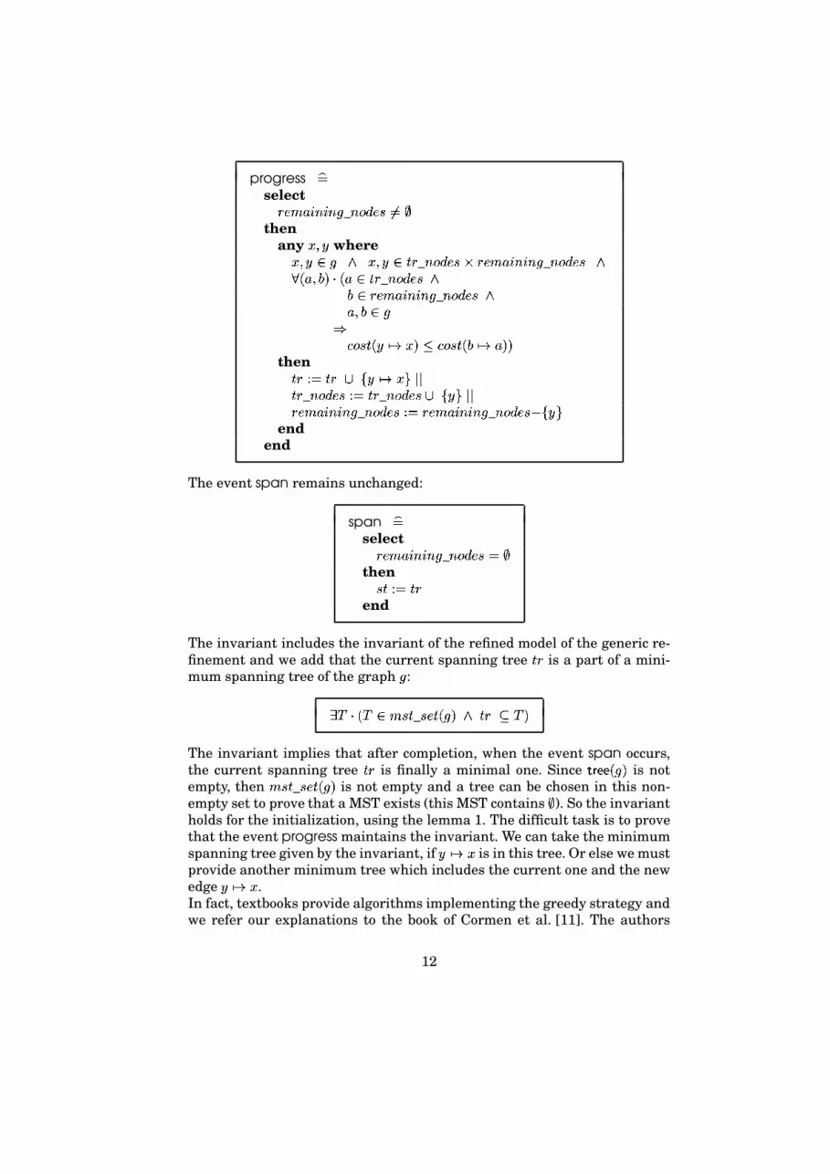
progress ¯&select���>ÄtÅ�{��²{h�2� _���������6Ì&0¥then

any �J!F� where�"!#�Î�<�Ís³�J!#�Î�t �� _ ���������Õ�Î���UÄ;Å�{��²{��2� _ ���������Þs£ �3Å,!�ïm$JB��3Å<�; �� _ ����������sï��Î���UÄ;Å�{��²{��2� _����������sÅ,!�ï��Î�w �`�*�> `� �6Ï�Ð�,$^î4�`�*�> `�)ï�Ï�äÅ�$F$then ��¨-8&4 ���È��>��Ï�ä���vºbº �� _ ����������-8&É �� _ ���������¹È'�>�,�IºQº���UÄtÅ�{��²{��2� _ ����������-8&É���UÄtÅ�{h�²{��2� _�������������>�,�end

end

The event span remains unchanged:

span ¯&select���UÄtÅ�{h�²{��2� _����������&0¥then�m A-8&9 ��end

The invariant includes the invariant of the refined model of the generic re-finement and we add that the current spanning tree �� is a part of a mini-mum spanning tree of the graph � :@ Û B�� Û �tÄt�> _ �U�U `�q�%$;s� ���� Û $The invariant implies that after completion, when the event span occurs,the current spanning tree �� is finally a minimal one. Since ·E�}¸m¸��q�%$ is notempty, then Ä��> _ �U�U `�q�%$ is not empty and a tree can be chosen in this non-empty set to prove that a MST exists (this MST contains ¥ ). So the invariantholds for the initialization, using the lemma 1. The difficult task is to provethat the event progress maintains the invariant. We can take the minimumspanning tree given by the invariant, if �6Ï�Ð� is in this tree. Or else we mustprovide another minimum tree which includes the current one and the newedge ��Ï�ä� .In fact, textbooks provide algorithms implementing the greedy strategy andwe refer our explanations to the book of Cormen et al. [11]. The authors

12

prove a theorem page 501 numbered 24.1 to assert that the choice of the twoedges is done following a given requirement, namely a safe edge (a safe edgeis a edge allowing the progress of the algorithm). We recall the theorem:

Theorem 1. (24.1, p 501from [11])Let � be a connected, undirected graph on � (set of nodes) with a real-valued weight function �`�*�> defined on � (edges). Let �� be a subset of � that isincluded in some minimum spanning tree for � , let � �� _ ����������!F���� �� _ ����������$be any cut of � that respects �� _ ��������� , and let � �"!#�%$ be a light edge crossing� �� _ ����������!F���� �� _ ���������U$ . Then edge �3�J!F��$ is safe for �� _ ��������� .

Let us explain notions of cut, crosses and light edge. A cut� �� _ ����������!F���� �� _ ���������U$F$ of an undirected graph � is a partition of � . Anedge � �"!#�%$ crosses the cut � �� _ ����������!F���� �� _ ����������$ if one of its endpoints isin �� _ ��������� and the other is in ���� �� _ ��������� . An edge is a light edge cross-ing a cut if its weight is the minimum of any edge crossing the cut. A lightedge is not unique.

Proof: LetÛ

be a minimum spanning tree that includes �� , and assume thatÛdoes not contain the light edge � �J!F�%$ , since if it does, we are done. We shall

construct another minimum spanning treeÛ K that includes ��ÎÈÖ�D� �J!F�%$Z� by

using a cut-and-paste technique, thereby showing that � �J!F�%$ is a safe edge for �� . The edge �3�J!#�%$ forms a cycle with the edges on the path | from � to � inÛ

.Since � and � are on opposite sides of the cut � �� _ ����������!F���� �� _ ����������$ , thereis at least one edge in

Ûon the path | that also crosses the cut. Let �3Å,!�ï`$ be

any such edge. The edge �3Å,!�ï`$ is not in �� , because the cut respects �� . Since(a,b) is on the unique path from � to � in

Û, removing �3Å,!�ïm$ breaks

Ûinto

two components. Adding �3�J!#�%$ reconnects them to form a new spanning treeÛ K�& Û �����)År!Zï`$Z��Èu��� �"!#�%$Z� . We next show thatÛ K is a minimum spanning

tree. Since �3�J!#�%$ is a light edge crossing � �� _ ����������!F���� �� _ ����������$ and �)År!Zï`$also crosses this cut, �`�*�> `�3�J!#�%$^î��`�*�> `�3Å,!�ïm$ . Therefore,���*�m `� Û K $¹&0���*�> `� Û $E�C�`�*�> `�)År!Zï`$Fí��m�*�m `�3�J!F��$î4���*�> `� Û $But

Ûis a minimum spanning tree, so that ���*�m `� Û $pîÞ���*�> `� Û Kb$ ; thus,

Û Kmust be a minimum spanning tree also. It remains to show that �3�J!#�%$ is ac-tually a safe edge for �� . We have ��Î� Û K , since ��<� Û

and �)Å,!�ï`$6ð�j �� ; thus, ���Èp�D� �"!#�%$Z��� Û K . Consequently, sinceÛ K is a minimum spanning tree, � �J!F�%$

is safe for �� . ñWe have to prove the property above that has been in fact adapted into theB proof engine. However, it is not a simple exercise of translation but a com-plete formulation of graph-theoretical aspects; moreover, the proof has beencompletely mechanized, as we will show in the next section. Let us com-pare the theorem and our formulation. The pair � �� _ ����������!F���� �� _ ����������$is a cut in the left part of the implication; the restriction of the tree æ tothe set of nodes �� _ ��������� is a tree rooted by � ; �3�J!#�%$ crosses the cut. Those

13

assumptions imply that there exists a spanning tree �#| rooted by � that isminimum on �� _ ��������� and such that there exists a light cut �)År!Zï`$ preservingthe minimality property.

We must give a formal description of this theorem. We introduce a predicateªU·E�b¸>¸�� ������ E!F����������!# �������$ stating that a structure ����U� is a tree on the set ���������and whose root is ������ :ªU·E�}¸m¸��3������ E!#����������!F �������$ɯ&°± ������ 9�ë��������� s ����U�á�Ó�������������>������ Z�(�,� ��������� s£2§ B�� § �è���������äs³������ ^� § s³ ����U� � �a¡ § ¢"� § w ����������& § $ µ¶Hence, we must add the following property which is proved separately.£ � Û !# �� _ ���������S!F�J!F��$NB�� �� _ �����������4�¤s�<�t��sªU·E�}¸m¸��3��!F��! Û $�¨�Î �� _ ����������s���t �� _ ����������s� �xð�Î �� _ ����������$;sªU·E�}¸m¸��3��!# �� _ ����������!>� �� _ �������������>����ò Û4ó �� _ ����������$F$;s£²À B�� À ���åsô�<� À s Û ¡ À ¢�� À w À ËN �� _ ���������áÌ&Í¥�$w @²�)År!Zï�! Û KQ$aBS�År!ZïC� Û sØÅpð�; �� _ ����������sØï��Î �� _ ����������sªU·E�b¸>¸�� ��!���! Û K $tsÛ K2�Æ� Û È Û � � ����ï^Ï�äÅ,!FŨÏ�´ïU��$,È��U�¨Ï�ä�J��s���*�m `� Û K}$f&0���*�> `� Û $E�C�`�*�> `�)ï�Ï�äÅ�$�í��`�*�> `� �¨Ï�Ã�,$ts��Ï�Ð��� Û K�s� �� _ ���������S���U���Cò Û4ó �� _ ����������$A� Û KQ$F$The property is the key result for ensuring the optimality of the greedystrategy in this process. In the next section, we detail the proof of our theo-rem.

6 On the theory of trees

As we have mentioned previously, trees play a central role in the justifica-tion of the algorithm; the optimality of the greedy strategy is mainly basedon the proof of the theorem used by Cormen et al. [11]. We should now detailthe theory of trees and intermediate lemmas required for deriving the theo-rem. Both the development of the tree identification protocol IEEE 1394 [3]

14

and the development of recursive functions [8] require proofs related to theclosure of relations; we apply the same technique for the closure of a func-tion defining a tree.Let � Û !F��$ be a tree defined by a tree function

Ûand a root � ; they satisfy the

following axioms ªU·E�}¸m¸�� ��!F��! Û $ .The closure �`õ of

Û � �is the smallest relation containing ¬ �,�3�<$ and stable

by application ofÛ � �

, that is:�`õN���³¾ ��s¬ �r�)�<$è�Ç�`õ�s�3�`õ#Ü Û � � $è�Ç�`õ�s£ ��B�� �¨�;�ö¾ ��s¬ �,�3�<$è�´��s� �DÜ Û � � $è�Ã�4sw �`õp�Ã�$Useful properties on the closure can be derived from those definitions; forinstance, the closure is a fix-point; the root � is connected to every node ofthe connected component; the closure is transitive, etc. We summarize thoseproperties using our notations:�`õ�&÷¬ �:�)�<$fÈ��3�`õ#Ü Û � � $EÜ���;�ë�4�`õ®Ü� Û � � Ü��`õ)$k�4�`õ®Ü�3�`õ#ÜF�`õh$A���`õ#ÜÛ Ë��`õ�&Ý¥�Ü�`õ�Ëp�`õ�� � �4¬ �,�3�<$`ÜFigure 1 contains a tree with the edge ïpÏ�øÅ and without the edge �ÝÏ�� . The construction of a new tree which contains the edge �4Ï�³� but notthe edge ï6Ï�åÅ is done according to the following points (see the result inFigure 3):

1. remove the edge ï�Ï�äÅ2. reverse all edges between � to ï (dashed arrows)3. add the edge �¨Ï�ä�

The resulting object seems to be a tree rooted by � . On Figure 2 we observethat the both parts are subtrees rooted by � or ï . We should prove these twofacts.

15

a

x

y

b

Fig. 1. A spanning tree containing ù>ú�ûa

x

y

b

Fig. 2. Two trees

a

x

y

b

Fig. 3. A spanning tree containing ü�ú�ý16

Lemma 3 (Concatenation of two separate trees)

LetÛ � !#� � !F � ! Û2þ !#� þ !F þ !F� be such that: ÿ�����

�����

ªU·E�}¸m¸��3� � !F � ! Û � $ªU·E�}¸m¸��3� þ !F þ ! Û²þ � Ëa þ &Ý¥ � Èa þ &0����� �Then ªU·E�b¸>¸�� � � !F��! Û � È Û þ Èk�U� þ Ï�Ð�J��$ .Proof Sketch: The proof is made up of several steps. A first step proves thatthe concatenation is a total function over the set � Èa þ

. A second one leadsto a more technical task and we should prove the inductive property overtrees using a splitting of the inductive variable

À(

À Ë� � andÀ Ë� þ

). ñLemma 4 (Subtree property)Let � Û !#�*$ be a tree on � ( ªU·E�}¸m¸�� ��!���! Û $ ) and ï a node in � .Then ªU·E�b¸>¸��)ï�!F�`õ ¡ ��ïU�m¢�!>�)�`õ ¡ ��ïU�>¢h����ïU�fò Û $#$Proof Sketch: The main difficulty is related to the inductive part. Wemust prove that, if

À � �`õ ¡ ��ïU�m¢ , ï�� Àand �3�mõ ¡ ��ïU�>¢h����ïU�6ò Û $ � ��¡ À ¢ �À

, then �`õ ¡ ��ïU�>¢�� À. We use the inductive property on

Ûwith the setÀ Èp���C�mõ ¡ ��ïU�>¢ . ñ

Lemma 5 (Complement of a subtree)Let � Û !#�*$ be a tree on � and ï a node in � .Then ªU·E�b¸>¸�� ��!����C�`õ ¡ ��ïU�m¢�!>�)�`õ ¡ ��ï��m¢��� Û $#$ .Proof Sketch: We should prove that, if

À � ���C�`õ ¡ ��ïU�m¢ , ïÆ� Àand�3�`õ ¡ ��ïU�m¢��� Û $ � ��¡ À ¢;� À

, then ���C�`õ ¡ ��ï��m¢6� À. A hint is to use the inductive

property onÛ

with the setÀ Èp�`õ ¡ ��ïU�m¢ . ñ

Now, we must characterize the subtree, where we have reversed the edgebetween � to the root ï . Let ���²ïZ �������� Û !�ïm$ be the subtree of

Ûwith ï as root

(it’s �`õ ¡ ��ïU�m¢�����ïU�kò Û). This following function seems to be a good choice:�)�`õ � ��¡ �>�,�m¢�� � ���²ïZ ����U�D� Û !�ï`$F$aÈ��)�`õ � ��¡ �>�,�m¢%ò����2ïE ������D� Û !�ï`$F$ � �

�3�`õ � ��¡ �>�,�>¢�ò;��²ïZ ������D� Û !Zï`$#$ � �is exactly all reverse edges. �`õ � �*¡ �U�r�>¢ is the set of

all parents of � .

Lemma 6 (Reverse from � to ï produces a tree)

Let ï�!#� such that: ï�����1���`õ ¡ ��ïU�m¢Then ªU·E�}¸m¸�� �2!F�mõ ¡ ��ïU�>¢h!U�3�`õ � �U¡ �>�,�m¢�� � ���²ïZ �������� Û !�ïm$#$NÈ��3�mõ � �*¡ �U�,�m¢Sò����2ïE ������D� Û !�ï`$F$ � � $Proof Sketch: In this case we must use an induction on the tree �`õ ¡ ��ïU�m¢ andsometimes use an second induction with the inductive property in hypothesis. ñ

17

Lemma 7 (Existence of a spanning tree)

Let Å,!Zï�!#�"!#� such that ÿ� �ï�!FÅ<� Û�<�t�`õ ¡ ��ï��m¢��-S���C�`õ ¡ ��ïU�>¢

Then there exists a treeÛ K such that:ÿ�����

�����

Û KÎ� � Û È Û � � ���UÅvÏ�Ãï�!�ï^Ï�äÅr��$dÈ��>��Ï�ä���ªU·E�}¸m¸��3��!F��! Û Kb$���*�> `� Û K}$f&Ý���*�m `� Û $E�C�m�*�m `�hïAÏ�ÃÅD$�í��`�*�> `� �6Ï�Ð�,$�¨Ï�Ð��� Û K�`õ ¡ ��ïU�m¢��� Û � Û KProof Sketch:

Û K is obtained by concatenation of . the two trees identifiedin the two previous lemmas. Both trees are linked by the edge �¨Ï�ä� . ñFinally, we have to prove the existence of an edge ï�Ï�äÅ which is safe in thesense of the greedy strategy.

Lemma 8 (Existence of ïAÏ�ÃÅ )

Let �� _ ����������!#� such that: ÿ��������������

�� _ ���������Æ�´��1������ �� _ ����������I�t �� _ ���������£²À B °± À ����s��Î� À s Û ¡ À ¢�� Àw À ËN �� _ ���������áÌ&Ñ¥ µ¶Then there exists Å and ï such that: ÿ���

���

Å1�; �� _ ���������ï^Ï�ÃÅ1� Ûï¨ð�; �� _ ���������ï��t�`õ � ��¡ �>�,�m¢ .

The property of the existence of a minimum spanning tree can now be de-rived using lemmas and the proof of the property is then completely mech-anized.

7 Related works

The refinement is a concept introduced by Back in his seminal paper [6] andit is developed from the wp semantics defined by E. Dijkstra [12]. Thoseseminal works inspire notations or methods for developing programs andsystems (Morgan[19], Abrial [1, 5], Gribomont [14] . . . ). Temporal aspectsare integrated into notations for extending the expressivity of the model-ing language (UNITY [9], TLA/TLA � [17, 18]). Clearly, our contribution isbased on the B event-based method, which is a proposal for an integratedmechanization of the refinement process and a methodology for develop-ing (reactive, distributed, sequential) systems; the B event-based approachproposes a complete environment supporting the methodological approach.However, as it was pointed out by previous readers, our works require com-parisons with development of MST-like systems using a formal framework.

18

First at all, Cormen et al. [11] present a collection of algorithms which arejustified in a pseudo-mathematical language, leaving details of formaliza-tion to the reader; we obtain a complete verified version of the algorithm.The paper of Stroetman [21] addresses a similar kind of case study, theconstrained minimal spanning tree problem, using the ASM [15] notation.Proofs are clearly done in a very classical way using the ASM mathematicalframework and no reference to the use of a proof tool is given. Moreover, ourcase study is related to Prim’s algorithm and we used an incremental pro-cess, namely the refinement. Although Stroetman mentions a refinement,it is not systematically used for constructing the final solutions. Fraer [13]has developed the Kruskal algorithm using the «classical» B method. In fact,the main difference is our use of the B event-based approach for develop-ing events systems. Even if Fraer has proved a part of proof obligations,it is clear that some proof obligations might be found false in the remain-ing unproved proof obligations. We recall that the goal of the refinement isto produce systems which are completely proved with respect to the targetproperties. Finally, we can reuse a part of our development for obtaining theKruskal algorithm.Our paper illustrates a systematic approach for developing event systemscombining the refinement and the proof process supported by a tool; formal-izations of concepts like graphs and trees are designed using the proof tooland are checked by the proof tool; they can be reused in other case studies.

8 Conclusion

The development of Prim’s algorithm leads us to state and to prove proper-ties over trees. The inductive definition of trees helps in deriving intermedi-ate lemmas asserting that the growing tree converges to the MST, accordingto the greedy strategy. The resulting algorithm is completely proved and wecan partially reuse current developed models to obtain Dijkstra’s algorithmor Kruskal’s one. The greedy strategy is not always efficient and the opti-mality of the resulting algorithm is proved by the theorem 24.1. The gainis clear, since we have a mechanized and verified proof of Prim’s algorithm.The mechanized proof looks like the proof given in the book of Cormen etal.; we think that it is a proof readable by specialists of graph theory. More-over, sketches of proofs are directly derived from the mechanized proofs; infact, the tool provides a way to discover these sketches. We can plan the re-writing of a book like Cormen et al including algorithms, complete develop-ments of each algorithm, proofs of developed algorithms and the possibilityto replay the developments to explain how each algorithm is really working.Future work will study other techniques related to algorithmics for graphtheory, since only one chapter in the book of Cormen et al. is treated!

19

References

1. J.-R. Abrial. A formal approach to large software constructions. In J. L. Avan de Snepscheut, editor, Mathematics for Program Construction, pages 1–20.Springer-Verlag, june 1989. LNCS 375.

2. J.-R. Abrial. Extending B without changing it (for developing distributed sys-tems). In H. Habrias, editor, 1 �� Conference on the B method, pages 169–190,November 1996.

3. J.-R. Abrial, D. Cansell, and D. Méry. A mechanically proved and incrementaldevelopment of the IEEE 1394 Tree Identify Protocol . Formal Aspects of Com-puting, ??(??), 2002. accepted for publication.

4. J.-R. Abrial and L. Mussat. Introducing dynamic constraints in B. In D. Bert,editor, B’98 :Recent Advances in the Development and Use of the B Method, vol-ume 1393 of Lecture Notes in Computer Science. Springer-Verlag, 1998.

5. J.R. Abrial. The B Book - Assigning Programs to Meanings. Cambridge Univer-sity Press, 1996. ISBN 0-521-49619-5.

6. R. J. R. Back. On correct refinement of programs. Journal of Computer andSystem Sciences, 23(1):49–68, 1979.

7. Dominique Cansell, Ganesh Gopalakrishnan, Mike Jones, Dominique Méry, andAiry Weinzoepflen. Incremental proof of the producer/consumer property for thepci protocol. In D. Bert, editor, ZB 2002, Lecture Notes in Computer Science.Springer-Verlag, January 2002.

8. Dominique Cansell and Dominique Méry. Développement de fonctions définiesrécursivement en b. Technical report, LORIA, 2002.

9. K. M. Chandy and J. Misra. Parallel Program Design A Foundation. Addison-Wesley Publishing Company, 1988. ISBN 0-201-05866-9.

10. ClearSy, Aix-en-Provence (F). Atelier B, 2002. Version 3.6.11. Thomas H. Cormen, Charles E. Leiserson, Ronald L. Rivest, and Cliff Stein. In-

troduction to Algorithms. MIT Press and McGraw-Hill, 2001.12. E. W. Dijkstra. A Discipline of Programming. Prentice-Hall, 1976.13. R. Fraer. Formal Development in B of a Minimum Spanning Tree Algorithm. In

H. Habrias, editor, 1 �� Conference on the B method, pages 169–190, November1996.

14. E. Pascal Gribomont. Concurrency without toil : a systematic method for paral-lel program design. Science of Computer Programming, 21:1–56, 1993.

15. Y. Gurevitch. Specification and Validation Methods, chapter "Evolving Algebras1993: Lipari Guide", pages 9–36. Oxford University Press, 1995. Ed. E. Börger.

16. J. B. Kruskal. On the shortest spanning subtree and the traveling salesmanproblem. Proc. Am. Math. Soc., 7:48–50, 1956.

17. L. Lamport. A temporal logic of actions. Transactions On Programming Lan-guages and Systems, 16(3):872–923, May 1994.

18. Leslie Lamport. Specifying Systems: The TLA+ Language and Tools for Hard-ware and Software Engineers. Addison-Wesley, 2002.

19. C. Morgan. Programming from Specifications. Prentice Hall International Se-ries in Computer Science. Prentice Hall, 1990.

20. R. C. Prim. Shortest connection and some generalizations. Bell Syst. Tech. J.,36, 1957.

21. K. Stroetmann. The constrained shortest path problem: A case study in usingASMs. J. of Universal Computer Science, 3(4):304–319, 1997.

20