arX

iv:1

210.

0090

v1 [

mat

h.C

O]

29

Sep

2012

The Number of Spanning Trees in Apollonian Networks

Zhongzhi Zhang, Bin Wu

School of Computer Science and Shanghai Key Lab of Intelligent Information Processing,

Fudan University, Shanghai 200433, China (zhangzz@fudan.edu.cn).

Francesc Comellas

Dep. Matematica Aplicada IV, EETAC, Universitat Politecnica de Catalunya, c/ EsteveTerradas 5, Castelldefels (Barcelona), Catalonia, Spain (comellas@ma4.upc.edu).

Abstract

In this paper we find an exact analytical expression for the number of span-ning trees in Apollonian networks. This parameter can be related to signif-icant topological and dynamic properties of the networks, including perco-lation, epidemic spreading, synchronization, and random walks. As Apol-lonian networks constitute an interesting family of maximal planar graphswhich are simultaneously small-world, scale-free, Euclidean and space fillingand highly clustered, the study of their spanning trees is of particular rel-evance. Our results allow also the calculation of the spanning tree entropyof Apollonian networks, which then we compare with those of other graphswith the same average degree.

Keywords: Apollonian networks, small-world graphs, complex networks,self-similar, maximally planar, scale-free

1. Introduction

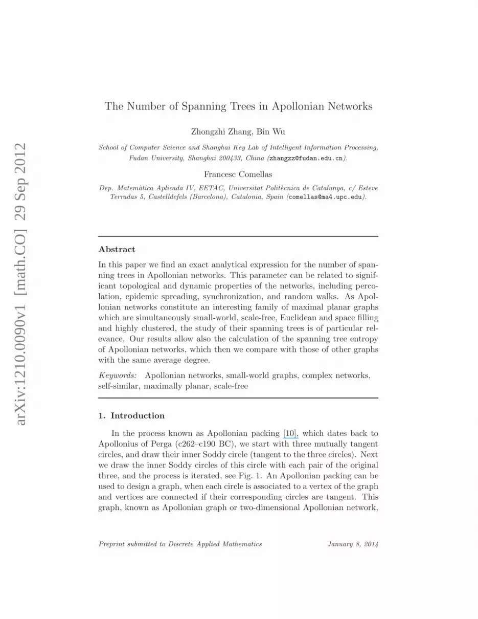
In the process known as Apollonian packing [10], which dates back toApollonius of Perga (c262–c190 BC), we start with three mutually tangentcircles, and draw their inner Soddy circle (tangent to the three circles). Nextwe draw the inner Soddy circles of this circle with each pair of the originalthree, and the process is iterated, see Fig. 1. An Apollonian packing can beused to design a graph, when each circle is associated to a vertex of the graphand vertices are connected if their corresponding circles are tangent. Thisgraph, known as Apollonian graph or two-dimensional Apollonian network,

Preprint submitted to Discrete Applied Mathematics January 8, 2014

was introduced by Andrade et al. [1] and independently proposed by Doyeand Massen in [7].

Apollonian networks have received much attention in recent years astwo-dimensional Apollonian networks are scale-free, small-world, maximallyplanar, Euclidean and space filling [1, 30]. Dynamical processes taking placeon these networks, such as percolation, epidemic spreading, synchronizationand random walks, have been also investigated, see [30, 28, 29, 11, 31].Some authors even suggest that the topological and dynamical properties ofApollonian networks are characteristic of neuronal networks as in the braincortex [17].

In this paper, we study the number of spanning trees of two-dimensionalApollonian networks. This study is relevant given the importance of thegraphs, and because the number of spanning trees of a finite graph is agraph invariant which characterizes the reliability of a network [6] and isrelated to its optimal synchronization and the study of random walks [14].The number of spanning trees of a graph can be obtained from the product ofall nonzero eigenvalues of the Laplacian matrix of the graph [9] (Kirchhoff’smatrix-tree theorem). However, although this result can be applied to anygraph, this calculation is analytically and computationally demanding.

Here, we follow a similar approach than for the Sierpinski gasket andHanoi graphs [5, 20, 21, 25] and our method to compute the number ofspanning trees in Apollonian networks is based on the self-similarity of thegraphs.

2. Apollonian networks

We recall in this section the definition and main topological properties oftwo dimensional Apollonian networks. We use standard graph terminologyand the words “network” and “graph” indistinctly.

Definition 2.1. An Apollonian network A(n), n ≥ 0, is a graph constructed

as follows:

For t = 0, A(0) is the complete graph K3 (also called a 3-clique or

triangle).For n ≥ 1, A(n) is obtained from A(n − 1): For each of the existing

subgraphs of A(n − 1) that is isomorphic to a 3-clique and created at step

n − 1, a new vertex is introduced and connected to all the vertices of this

subgraph. Figure 2 shows this construction process.

We note that Apollonian networks belong to the family of graphs knownas k-trees, introduced in the 1970s [4], and which have been extensively

2

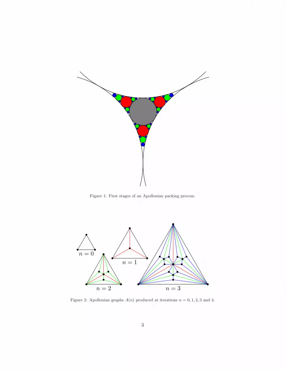
Figure 1: First stages of an Apollonian packing process.

n = 0

n = 1

n = 2 n = 3

Figure 2: Apollonian graphs A(n) produced at iterations n = 0, 1, 2, 3 and 4.

3

studied since. They are defined as follows: a k-clique is a k-tree; if G is a k-tree, adding a vertex to G and joining it to all vertices of an existing k-cliquein G yields a new graphG′, which is also a k-tree. Thus, Apollonian networksare k-trees, since they start with a 3-clique (that is, the only possible k-treewith 3 vertices), and since each time a vertex is added, it is joined to all thevertices of an existing 3-clique. k-trees are of interest as they are maximalgraphs for a given tree-width.

Thanks to the deterministic nature of the graphs A(n), it is possible togive exact values for relevant topological properties of these graphs, includ-ing degree distribution, degree correlations, clustering, diameter and averagedistance.

Order and size of A(n).– The order and size of an Apollonian graph A(nare Vn = |V (n)| = 1

2 (3n + 5) and En = |E(n)| = 3

2(3n + 1).

Planarity– A graph is planar if it can be drawn on the plane with noedges crossing. A planar graph is maximal, or maximally planar, if it cannotbe extended to a larger planar graph by adding an edge.

Apollonian networks are maximally planar [1] and this is an importantfeature for its relevance in the development of efficient algorithms [3].

Degree distribution.– The cumulative degree distribution of an Apollo-nian network A(n) is P (k) ∝ k1−γ . with γ = ln 3/ ln 2 = 2.58496, see[1, 7]. The graph is scale-free. Many real networks share this property withexponent values in the same range as A(n) [15].

Correlation coefficient.– From the Pearson correlation coefficient for thedegrees of the endvertices of the edges of A(n), Doye and Massen ob-tained in [7] the exact value of the correlation coefficient and it is alwaysnegative and thus the network is disassortative. For large values of n,r(n) ∼ −10

3

(

23

)n. Thus, this parameter goes to zero as the order of the

graph increases. Technological and biological networks are usually disassor-tative as it is also the case of some information networks, see [15, 19].

Modularity and self-similarity.– From Fig. 2, we see that Apolloniannetworks are self-similar, suggesting an alternative way to construct them.As shown in Fig. 3, A(n + 1) can be obtained by joining three replicas ofA(n), labeled by A1

n, A2n and A3

n, and identifying three pairs of edges. Thus,the graphs are modular. Modularity can be quantified with the functionQ introduced by Newman and Girvan [16]. For Apollonian networks Q =0.5938. Moreover, the communities are spatially localized [1, 7].

4

A1

n A2

n

A3n

A1

n A2

n

A3

n

A(n +1)

Figure 3: Recursive construction of Apollonian networks, pointing out their self-similarity.A(n+ 1) can be obtained by joining three replicas of A(n), labeled here A1

n, A2

nand A3

n,

after merging three pairs of edges.

Clustering.– The clustering coefficient C of A(n) is 0.8284 for large n.Furthermore, the clustering coefficient of a vertex of A(n), for large n, is

inversely proportional to its degree [1, 28]: C(k) =4(k − 3

2)

k(k − 1). This property

is considered to be a signature of a hierarchical network structure, see [2]

Average distance and diameter.– The modular recursive construction ofA(n) allows to obtain the exact analytical value for its average distance [24].The average distance of A(n), for n large, follows d(n) ∼ ln |Vn| which showsa logarithmic scaling with the order of the graph. As the diameter has asimilar behavior [23], the graph is small-world.

3. The number of spanning trees in Apollonian networks

In this section, we find the number of spanning trees of the Apolloniannetwork A(n). For this calculation we use a decimation method [12] whichhas been used to find the number of spanning trees in other recursive graphfamilies like the Sierpinski gasket [5], the pseudofractal web [26], and somefractal lattices [27]. The particular structure of Apollonian networks, allowus to write recursive equations for the number of spanning trees which aresolved by induction.

In the following, we denote by Vn and En the number of vertices andedges of A(n). Then a spanning subgraph of A(n) is a subgraph with thesame vertex set as A(n) and a number of edges E′

n such that E′

n ≤ En.A spanning tree of A(n) is a spanning subgraph which is a tree and thusE′

n = Vn − 1.We call “hub vertices” the three outmost vertices in the construction as

5

shown in Fig. 2 and “hub edges” the three exterior edges which connect thehub vertices.

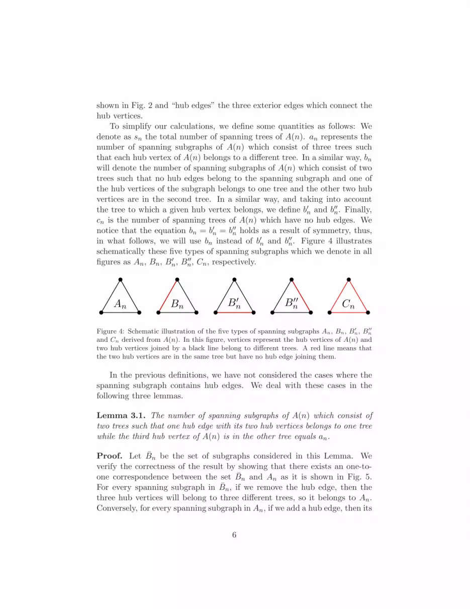
To simplify our calculations, we define some quantities as follows: Wedenote as sn the total number of spanning trees of A(n). an represents thenumber of spanning subgraphs of A(n) which consist of three trees suchthat each hub vertex of A(n) belongs to a different tree. In a similar way, bnwill denote the number of spanning subgraphs of A(n) which consist of twotrees such that no hub edges belong to the spanning subgraph and one ofthe hub vertices of the subgraph belongs to one tree and the other two hubvertices are in the second tree. In a similar way, and taking into accountthe tree to which a given hub vertex belongs, we define b′n and b′′n. Finally,cn is the number of spanning trees of A(n) which have no hub edges. Wenotice that the equation bn = b′n = b′′n holds as a result of symmetry, thus,in what follows, we will use bn instead of b′n and b′′n. Figure 4 illustratesschematically these five types of spanning subgraphs which we denote in allfigures as An, Bn, B

′

n, B′′

n, Cn, respectively.

An BnB′

nB′′

n Cn

Figure 4: Schematic illustration of the five types of spanning subgraphs An, Bn, B′

n, B′′

n

and Cn derived from A(n). In this figure, vertices represent the hub vertices of A(n) andtwo hub vertices joined by a black line belong to different trees. A red line means thatthe two hub vertices are in the same tree but have no hub edge joining them.

In the previous definitions, we have not considered the cases where thespanning subgraph contains hub edges. We deal with these cases in thefollowing three lemmas.

Lemma 3.1. The number of spanning subgraphs of A(n) which consist of

two trees such that one hub edge with its two hub vertices belongs to one tree

while the third hub vertex of A(n) is in the other tree equals an.

Proof. Let Bn be the set of subgraphs considered in this Lemma. Weverify the correctness of the result by showing that there exists an one-to-one correspondence between the set Bn and An as it is shown in Fig. 5.For every spanning subgraph in Bn, if we remove the hub edge, then thethree hub vertices will belong to three different trees, so it belongs to An.Conversely, for every spanning subgraph in An, if we add a hub edge, then its

6

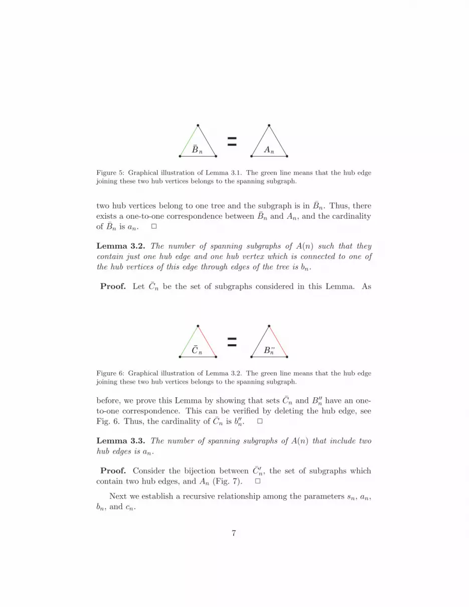
B n An=Figure 5: Graphical illustration of Lemma 3.1. The green line means that the hub edgejoining these two hub vertices belongs to the spanning subgraph.

two hub vertices belong to one tree and the subgraph is in Bn. Thus, thereexists a one-to-one correspondence between Bn and An, and the cardinalityof Bn is an. ✷

Lemma 3.2. The number of spanning subgraphs of A(n) such that they

contain just one hub edge and one hub vertex which is connected to one of

the hub vertices of this edge through edges of the tree is bn.

Proof. Let Cn be the set of subgraphs considered in this Lemma. As

C n B”n=

Figure 6: Graphical illustration of Lemma 3.2. The green line means that the hub edgejoining these two hub vertices belongs to the spanning subgraph.

before, we prove this Lemma by showing that sets Cn and B′′

n have an one-to-one correspondence. This can be verified by deleting the hub edge, seeFig. 6. Thus, the cardinality of Cn is b′′n. ✷

Lemma 3.3. The number of spanning subgraphs of A(n) that include two

hub edges is an.

Proof. Consider the bijection between C ′

n, the set of subgraphs whichcontain two hub edges, and An (Fig. 7). ✷

Next we establish a recursive relationship among the parameters sn, an,bn, and cn.

7

¯ =C’n An

Figure 7: Graphical illustration of Lemma 3.3. The green line means that the hub edgejoining these two hub vertices belongs to the spanning subgraph .

Lemma 3.4. For n ≥ 0, an+1 = 3a3n + 6a2nbn.

Proof. We prove this result by considering a graphical version of the equa-tion (Fig. 8) which represents the recursive construction method of A(n+1)from A(n) and enumerates all possible contributions to an+1.

In this representation we only draw four vertices in each case, since eachnon drawn (interior) vertex connects at least to one of these four vertices(although they do not have necessarily to be adjacent). This is sufficient todetermine whether each case belongs to An+1, Bn+1 or Cn+1 .

= ×3+ ×6

Figure 8: Configurations needed to find an+1 from an and bn. In this representation, thered curve denotes the spanning tree to which the two hub vertices belong to. The numberon the right of the figure counts configurations that, by symmetry, contribute to an+1

through the merging process

Next we should prove that each configuration is correct, but we onlyanalyze in detail the first additive term as the other term can be verifiedin a similar way. For this case (see Fig. 9), hub vertices h1 and h4 areconnected while h2 and h3 are not. Thus, after merging, there are threespanning trees and we confirm that this subgraph belongs to An+1. Becauseof the symmetry, h4 can also be connected to h2 or h3 and we count threetimes this case. ✷

Lemma 3.5. For n ≥ 0, bn+1 = a3n + 7a2nbn + 7anb2n + a2ncn.

Proof. We prove the lemma by enumeration. Figure 10 shows all the

8

h1

h4

h3h2

Figure 9: The first configuration which contributes to an+1.

= + ×2+ ×2+ + + ×2

+ ×2+ ×2+ ×2+

Figure 10: Configurations needed to find bn+1.

distinct possibilities. Again, we only analyze the first case. We label thefour hub vertices in the same way as in Fig. 9. In the first case, h1, h2, h4are all connected while h3 is not. There are two spanning trees, and onehas no hub edges, so this configuration belongs to set Bn+1. Symmetriesgenerate equivalent configurations and the factor is one. ✷

Lemma 3.6. For n ≥ 0, cn+1 = a3n + 12a2nbn + 36anb2n + 14b3n + 3a2ncn +

12anbncn.

Proof. As in former lemmas, the proof is by enumeration of all possiblecontributions to cn+1, see in Fig. 11 the details. In the first case, h1, h2, h3and h4 are all connected and the merging process produces a spanning tree.As no hub edges are included in it, we can see that this case belongs to setCn+1. Besides, because of the symmetry, only this configuration is relevant.All other cases are analyzed similarly and we omit the details. ✷

Lemma 3.7. For n ≥ 0, sn+1 = 16a3n + 72a2nbn + 78anb2n + 14b3n + 9a2ncn +

12anbncn.

Proof. Figure 12 shows all the configurations contributing sn+1. We donot give the calculation details as they are like in former lemmas. ✷

9

= + ×6+ ×6+ ×3+ ×6+ ×6

+ ×3+ ×6+ ×6+ ×6+ ×3+ ×6

+ ×6+ ×2+ ×6+ ×6

Figure 11: Configurations that contribute to cn+1.

= + ×6+ ×3+ ×6+ ×6+ ×6

+ ×6+ ×6+ ×6+ ×6+ ×6+ ×6

+ ×6+ ×6+ ×6+ ×6+ ×3+ ×6

+ ×6+ ×6+ ×6+ ×6+ ×6+ ×6

+ ×3+ ×6+ ×6+ ×6+ ×6+ ×6

+ ×6+ ×3+ ×6+ ×6+ ×2+ ×6

+ ×6

Figure 12: Illustration for the calculation of sn+1. Here, a blue line indicates that thecorresponding hub vertices belong to the same spanning tree (including both the caseswhere they are adjacent and they are connected through other vertices).

10

Lemma 3.8. For n ≥ 0, ancn = 3b2n.

Proof. By induction. For n = 0, using the initial conditions a0 = 1, b0 = 0and c0 = 0, the result is true.

Then we assume that for n = k, the lemma is true. For n = k + 1, andusing Lemmas 3.4-3.6, we have that

ak+1ck+1 − 3b2k+1 = (3a3k + 6a2kbk)(a3k + 12a2kbk + 36akb

2k + 14b3k + 3a2kck

+12akbkck)− 3(a3k + 7a2kbk + 7akb2k + a2kck)

2

= 3a2k(a2k + 4akbk + 7b2k − akck)(akck − 3b2k) ,

As by induction hypothesis, we have that akck − 3b2k = 0 we obtain theresult. ✷

Lemma 3.9. For n ≥ 0, an+1

a3n

= 5n

3n−1 .

Proof. Define fn = an+1

a3n

. From Lemma 3.4, we have

an+1

a3n=

3a3n + 6a2nbna3n

= 3 + 6bnan

,

and thusbnan

=1

6

(

an+1

a3n− 3

)

.

We use Lemmas 3.8 and 3.5, to obtain:

bn+1

a3n= 1 + 7

bnan

+ 10

(

bnan

)2

= 1 + 7

[

1

6

(

an+1

a3n− 3

)]

+ 10

[

1

6

(

an+1

a3n− 3

)]2

= −an+1

2a3n+

5a2n+1

18a6n,

which gives:

bn+1

an+1=

bn+1

a3n

a3nan+1

=

(

−an+1

2a3n+

5a2n+1

18a6n

)

a3nan+1

= −1

2+

5an+1

18a3n.

Thusan+2

a3n+1

= 3 + 6bn+1

an+1= 3 + 6

(

−1

2+

5an+1

18a3n

)

=5an+1

3a3n,

11

which we can write as

fn+1 =5

3fn.

From the initial condition f0 =a1a30

= 3 = 50

3−1 , we finally find

fn =an+1

a3n=

5n

3n−1.

✷

Lemma 3.10. For n ≥ 0, an = 3−1

4+ 3

n

4+n

2 5−1

4+ 3

n

4−

n

2 .

Proof. From the former Lemma we have an+1 =5n

3n−1 a3n, which with initial

condition a0 = 1 gives

an = 3−1

4+ 3

n

4+n

2 5−1

4+ 3

n

4−

n

2 .

✷

Lemma 3.11. For n ≥ 0, bn = 1215

1

4(−1+3n−2n)(5n − 3n).

Proof. From Lemma 3.4 we know that bn = an+1−3a3n

6a2n

and using Lemma 3.10

we obtain

bn =1

215

1

4(−1+3n−2n)(5n − 3n).

✷

Lemma 3.12. For n ≥ 0, cn = 143

1

4(3+3n−6n)5

1

4(−1+3n−2n) (3n − 5n)2.

Proof. According to Lemma 3.8, we have cn = 3b2n

an, and using the results

of Lemmas 3.10 and 3.11, we obtain

cn =1

43

1

4(3+3n−6n)5

1

4(−1+3n−2n) (3n − 5n)2 .

✷

Theorem 3.13. The number of spanning trees of A(n) is

sn =1

43

3

4(−1+3n−1

−2(n−1))51

4(−3+3n−2(n−1))(3n + 5n)2.

12

Proof. The result comes from Lemmas 3.7, 3.10, 3.11 and 3.12. ✷

After having an explicit expression for the number of spanning treesof A(n), we can calculate its spanning tree entropy, which is defined asin [22, 13]:

z = limn→∞

ln snVn

.

The spanning tree entropy is an interesting parameter charactering thenetwork structure.

Corollary 3.14. The spanning tree entropy of Apollonian networks isln 15

2.

Proof. Define zn = ln snVn

. From Theorem 3.13, we have

zn =−8 ln 2 + ln 27

5 + 3n ln 15− 2n ln 135 + 8 ln(3n + 5n)

2(5 + 3n),

and finally

z = limn→∞

zn =ln 15

2.

✷

We can compare this asymptotic value of the entropy of the spanningtrees for Apollonian networks, z = ln 15

2 ≃ 1.3540, with that of other graphswith the same average degree. For example, the value for the Sierpin-ski graph is 1.5694 [5] and for the 3-dimensional hypercubic lattice L3 is1.6734 [18, 8]. Thus, the asymptotic value for Apollonian networks is thelowest reported for graphs with average degree 6. This reflects the fact thatthe number of spanning trees in A(n), although growing exponentially, doit at a lower rate than graphs with the same average degree.

4. Conclusion

In this paper we find the number of spanning trees in Apollonian net-works by using a method, based on its self-similar structure, which allowsus to obtain an exact analytical expression for any number of discs. Themethod could be used to further study in this graph, and other self-similargraphs, their spanning forests, connected spanning subgraphs, random walksand vertex or edges coverings. Knowing the number of spanning trees forApollonian networks allows us to show that their spanning tree entropy islower than in other graphs with the same average degree.

13

Acknowledgements

Z. Zhang is supported by the National Natural Science Foundation ofChina under Grants No. 61074119. F. Comellas is supported by the Minis-terio de Economia y Competitividad, Spain, and the European Regional De-velopment Fund under project MTM2011-28800-C02-01 and partially sup-ported by the Catalan Research Council under grant 2009SGR1387.

References

[1] J. S. Andrade Jr., H. J. Herrmann, R. F. S. Andrade, L. R. daSilva, Apollonian Networks: Simultaneously scale-free, small world, Eu-clidean, space filling, and with matching graphs, Phys. Rev. Lett. 94(2005) 018702.

[2] A. L. Barabasi, Z.N. Oltvai , Network biology: Understanding the cell’sfunctional organization, Nat. Rev. Genet. 5 (2004) 101-114.

[3] A. Brandstadt, V. B. Le, J. P. Spinrad . Graph Classes: A Sur-vey (SIAM Monographs on Discrete Mathematics and Applications)Philadelphia, PA, 1999.

[4] L.W. Beineke, R.E. Pippert, Properties and characterization of k-trees,Mathematika 18 (1971) 141–151.

[5] S.-C. Chang, L.-C. Chen, W.-S. Yang, Spanning trees on the Sierpinskigasket, J. Stat. Phys. 126 (2007) 649–667.

[6] C.J. Colbourn, The Combinatorics of Network Reliability, New York,Oxford University Press 1987.

[7] J. P. K. Doye, C. P. Massen, Self-similar disk packings as model spatialscale-free networks, Phys. Rev. E 71 (2005) 016128.

[8] J.H. Felker, R. Lyons, High-precision entropy values for spanning treesin lattices, J. Phys. A: Math. Gen. 36 (2003) 83618365.

[9] C. Godsil, G. Royle, Algebraic Graph Theory, Graduate Texts in Math-ematics 207, Springer, New York 2001.

[10] E. Kasner, F.D Supnick, The Apollonian packing of circles, Proc. Natl.Acad. Sci. U.S.A. 29 (1943) 378–384.

14

[11] Z-G. Huang, X-J. Xu, Z-X. Wu, Y.H. Wang, Walks on Apolloniannetworks, Eur. Phys. J. B 51 (2006) 549–553.

[12] M. Knezevic, J. Vannimenus, Large-scale properties and collapse tran-sition of branched polymers: Exact results on fractal lattices, Phys.Rev. Lett. 56 (1986) 1591.

[13] R. Lyons, Asymptotic enumeration of spanning trees, Combin. Probab.Comput. 14 (2005) 491–522.

[14] P. Marchal, Loop-erased random walks, spanning trees and hamiltoniancycles, Elect. Comm. in Probab. 5 (2000) 39-50.

[15] M.E.J. Newman, The structure and function of complex networks,SIAM Review 45 (2003) 167–256.

[16] M. E. J. Newman and M. Girvan, Finding and evaluating communitystructure in networks, Phys. Rev. E 69 (2004) :026113.

[17] G.L. Pellegrini, L. de Arcangelis, H.J. Herrmann, C. Perrone-Capano.Modelling the brain as an Apollonian network, arXiv:q-bio/0701045v1,2007.

[18] R. Shrock and F. Y. Wu, Spanning trees on graphs and lattices in ddimensions, J. Phys. A: Math. Gen. 33 (2000) 3881.

[19] R. V. Sole, S. Valverde, Information theory of complex networks: onevolution and architectural constraints, Lecture Notes in Phys. 650(2004) 189–207.

[20] E. Teufl, S. Wagner, Resistance scaling and the number of spanningtrees in self-similar lattices, J. Stat. Phys. 142 (2011) 879–897.

[21] E. Teufl, S. Wagner, The Number of Spanning Trees in Self-SimilarGraphs, Ann. Comb. 15 (2011) 355–380.

[22] F. Y. Wu, Number of spanning trees on a lattice, J. Phys. A: Math.Gen. 10 (1977) 113-115.

[23] Z. Zhang, F. Comellas, G. Fertin, L. Rong, High dimensional Apollo-nian networks, J. Phys. A 39 (2006) 1811–1818.

[24] Z. Zhang, L. Chen, S. Zhou, L. Fang, J. Guan, T. Zou, Analyticalsolution of average path length for Apollonian networks, Phys. Rev. E77 (2008) 017102.

15

[25] Z. Zhang, S. Wu, F. Comellas, The number of spanning trees of Hanoigraphs, submitted.

[26] Z. Zhang, H. Liu, B. Wu, S. Zhou, Enumeration of spanning trees in apseudofractal scale-free web, Europhys. Lett. 90 (2010) 68002.

[27] Z. Zhang, H. Liu, B. Wu, T. Zou, Spanning trees in a fractal scale-freelattice, Phys. Rev. E 83 (2011) 016116.

[28] Z. Zhang, L. Rong, F. Comellas, High dimensional random Apolloniannetworks, Physica A 364 (2005) 610–618.

[29] Z. Zhang, L. Rong, S.G. Zhou, Evolving Apollonian networks withsmall-world scale-free topologies, Phys. Rev. E 74 (2006) 046105.

[30] T. Zhou, G. Yan, and B.H. Wang, Maximal planar networks with largeclustering coefficient and power-law degree distribution, Phys. Rev. E71 (2005) 046141.

[31] Z. Zhang, S. Zhou, Correlations in random Apollonian networks, Phys-ica A 380 (2007) 621–628.

16