F ti V l tilit f UKForecasting Volatility of UK natural gas futuresg

Robert A Yaffee New York University NYC NYRobert A. Yaffee, New York University, NYC,NYMerrill A. Heddy, Heddy Consultants LLC East Rutherford, NJ

Sjur Westgaard, Trondheim Business School and Norwegian University of Science and Technology Trondheim, Norway

Kai Hjemgaard student Norwegian University of Science and Technology, Trondheim, Norway

Bjorn Helge Bore student Norwegian University of Science and Technology, Trondheim, Norway

Joseph I. Onochie, Baruch College CUNY, NYC,NY

International Symposium on ForecastingNice, FranceJune 2008

E-mail addressesE mail addresses

• Robert A Yaffee yaffee@nyu eduRobert A. Yaffee, yaffee@nyu.edu• Merrill A. Heddy,

heddy consultants@yahoo comheddy_consultants@yahoo.com• Sjur Westgaard sjur.westgaard@hist.no• Kai Hjemgaard, post@bhbore.no• Bjorn Helge Bore, post@bhbore.noj g , p @• Joseph I. Onochie

Joseph Onochie@baruch cuny eduJoseph_Onochie@baruch.cuny.edu2

AcknowledgmentsAcknowledgments

• The authors would like to thank Prof SebastienThe authors would like to thank Prof. Sebastien Laurent for his tutelage and gracious assistance in our research.

• We also would like to thank Dr. Jurgen Doornik for his excellent instruction in the Oxfor his excellent instruction in the Ox programming language.

• We would also like to thank Kate Hancock at ICEWe would also like to thank Kate Hancock at ICE Data for assistance in supplying the data and Ana Timberlake for administrative assistance.

3

OutlineOutline

1 Motivation1. Motivation2. Background3 h bl3. Research problems4. Data5. Methods6 Results and Discussion6. Results and Discussion7. Conclusions

4

MotivationMotivation

• Previous research has focused on US naturalPrevious research has focused on US natural gas futures

• There is reason to believe that the UK situationThere is reason to believe that the UK situation is different from that of the US

• There have been very few attempts to model,There have been very few attempts to model, much less, forecast UK natural gas futures

• We apply new techniques for this particularWe apply new techniques for this particular geographical area.

• We try to fill the knowledge gapWe try to fill the knowledge gap

5

Motivation continuedMotivation continued

• Why this is important?Why this is important?– There is insecurity in resource supply during the

winterwinter.– Volatility estimation and forecasting is necessary

for reserve requirement planning.for reserve requirement planning.– Volatility estimation and forecasting is necessary

for defining Value-at-Risk (VaR) quantiles, VaR g ( ) q ,accuracy, and expected shortfall.

– VaR is now a standard means of assessing risk. g

6

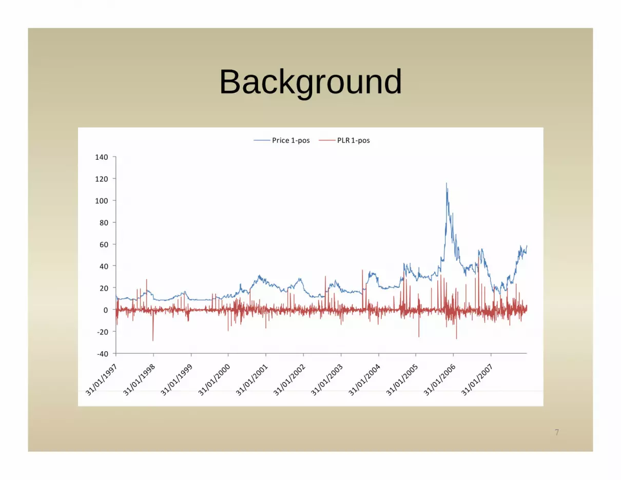
BackgroundBackgroundPrice 1‐pos PLR 1‐pos

100

120

140

40

60

80

20

0

20

‐40

‐20

7

BackgroundBackground• Deregulation has led to calls for redefinition of risk in the

1990s in this market.• Linkage to the European Interconnector and North Sea

pipelines distinguishes this market from that of the U.S. situation where most of the previous research on volatility was focused.

• Insecurity of supply during winter months has increased y pp y gvolatility.

• Volatility increases reserve requirements and general demand.

• 45% of UK electricity in 2007 came from natural gas supplies, so this is an important factor of production and consideration in the cost of living in the U.K.g

8

Research problemsResearch problems1. Can we model UK natural gas futures with1. Can we model UK natural gas futures with

GARCH models?2. What are the best models for all positions?p3. How valid are these models?4. How stable are these models?5. How does volatility affect percentage log

returns?6. Which models forecast best for each of 9

positions over 1, 5, 10 and 20 trading days?

9

DataData

• Time frame: 1997 thru 2007Time frame: 1997 thru 2007• Unit for analysis of price: GBPence/therm

il l 100*(l ( ) / ))• Daily percentage log returns: 100*(ln(P)t/Pt-1))• 9 months positions (postponed 1 through 9

months)• Data from Inter-Continental Exchange (ICE)g ( )

10

Methods 1Methods 1

• Preliminary AnalysisPreliminary Analysis– ACF, PACF of PLR suggest occasionally AR(1) or

AR(1/2)( )– ADF tests suggest mean (not necessarily variance)

stationarity of PLR.– Geweke Porter Hudak tests suggest no long memory– Sign-bias tests generally indicate no asymmetry

• GARCH mining– Based on lowest Schwartz Criterion

11

Methods 2Methods 2

• Residual diagnosticsResidual diagnostics– Portmanteau tests of standardized residuals

Portmanteau tests of squared residuals– Portmanteau tests of squared residuals– Tse’s Residual Based Diagnostics test

• Nyblom stability tests

2 2 21 1 2 2( 1) ... p

t t t t pE z z zα α α− − −− = + + +

– Individual and joint tests were run.

12

RiskMetrics ModelRiskMetrics Model

2p q

mean model :

l l Rφ θ δ δ∑ ∑ 21 2

1 1t i t i j t j t t t

i j

plr c plr Rφ θ ε δ σ δ ε− −= =

= + − + + +∑ ∑

2 2 21 1(1 )t t t t

RiskMetrics variance model :bRσ ω λ ε λσ− −= + − + +

wherec constant=

~ . . . (0,1, )( / )

t t t

t

zz i i d t vR contract rollover dummy last working day month

ε σ=

( / )tR contract rollover dummy last working day month=

130.94λ =

RiskMetrics Forecasting ModelRiskMetrics Forecasting Model

:mean forecasting model

2| | | 1 | 2 |

1 1

p q

t h t i t h i t j t h j t t h t t h t ti j

plr c plr Rφ θ ε δ σ δ ε+ + − + − + += =

= + − + + +∑ ∑

:RiskMetrics variance forecasting model2 2 2

| 1| 1| |(1 )

1 5 10t h t t h t t h t t h t

f gbR

h h f t h i f d

σ ω λ ε λσ+ + − + − += + − + +

20 l d1,5,10,where h forecast horizon of and= 20 leads14

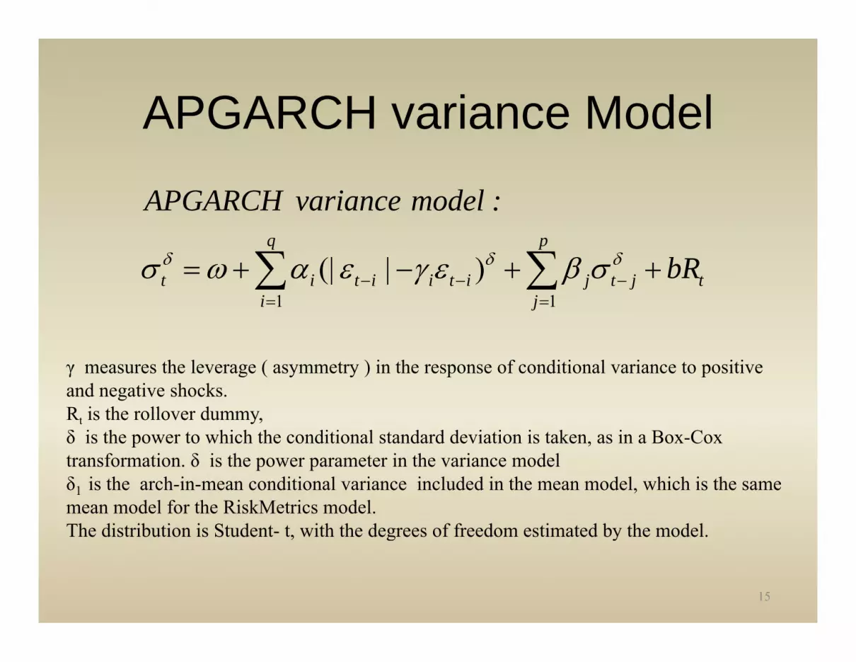
APGARCH variance ModelAPGARCH variance Model

APGARCH variance model :

(| | )q p

t i t i i t i j t j t

APGARCH variance model :

bRδ δ δσ ω α ε γ ε β σ− − −= + − + +∑ ∑1 1

j ji j= =∑ ∑

γ measures the leverage ( asymmetry ) in the response of conditional variance to positiveγ measures the leverage ( asymmetry ) in the response of conditional variance to positive and negative shocks. Rt is the rollover dummy, δ is the power to which the conditional standard deviation is taken, as in a Box-Cox t f ti δ i th t i th i d ltransformation. δ is the power parameter in the variance model δ1 is the arch-in-mean conditional variance included in the mean model, which is the same mean model for the RiskMetrics model. The distribution is Student- t, with the degrees of freedom estimated by the model., g y

15

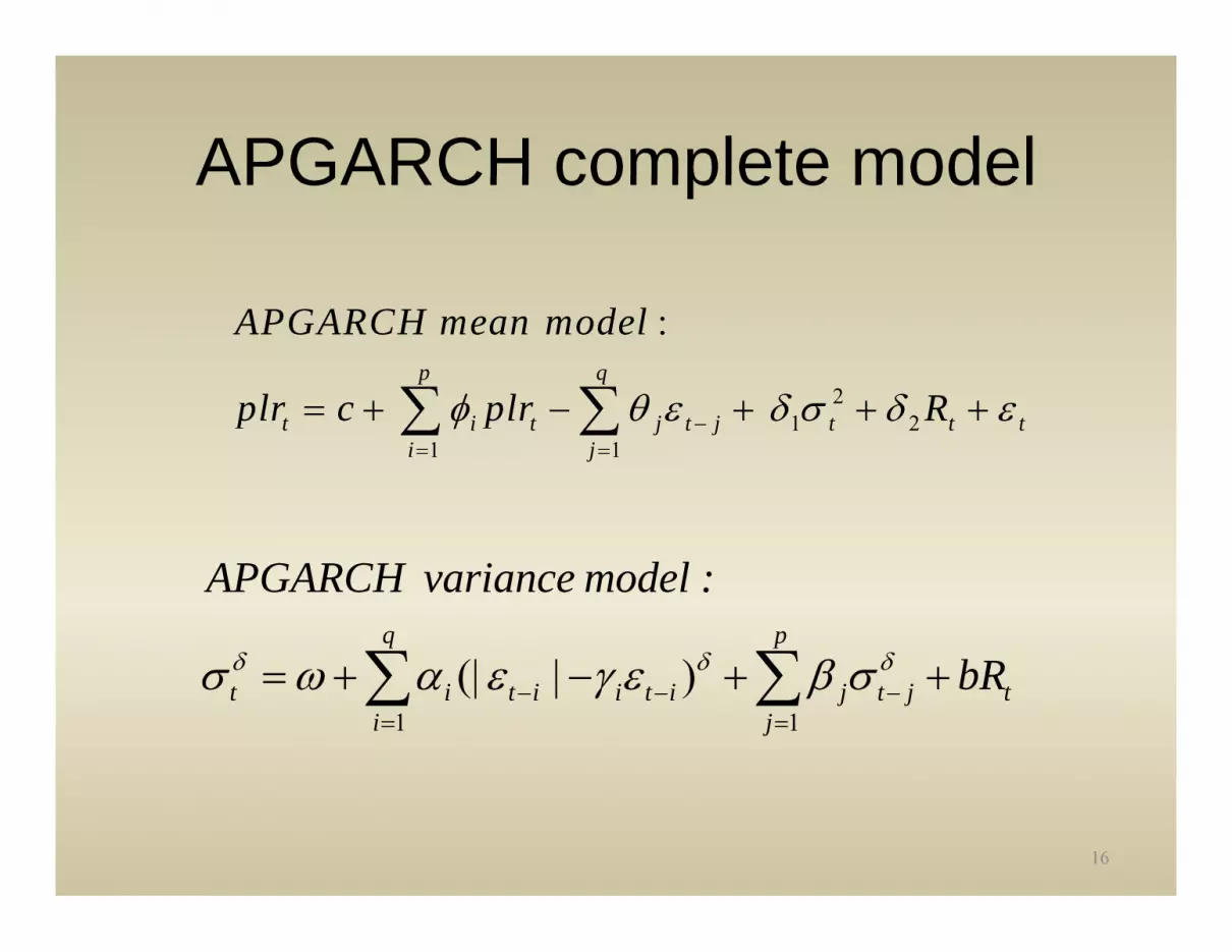
APGARCH complete modelAPGARCH complete model

21 2

:p q

APGARCH mean model

plr c plr Rφ θ ε δ σ δ ε= + − + + +∑ ∑ 1 21 1

t i t j t j t t ti j

plr c plr Rφ θ ε δ σ δ ε−= =

+ + + +∑ ∑

q p

APGARCH variance model :

δ δ δ∑ ∑1 1

(| | )t i t i i t i j t j ti j

bRδ δ δσ ω α ε γ ε β σ− − −= =

= + − + +∑ ∑

16

APGARCH Forecasting modelAPGARCH Forecasting model

2| | | 1 | 2 | |

p q

t h t i t h i t j t h j t t h t t h t t h t

APGARCH mean forecasting model :

plr c plr Rφ θ ε δ σ δ ε+ + − + − + + += + + + + +∑ ∑| | | 1 | 2 | |1 1

:

t h t i t h i t j t h j t t h t t h t t h ti j

q p

APGARCH variance forecasting model

+ + + + + += =∑ ∑

| | | | |1 1

(| | )q p

t h t i t h i t i t h i t j t h j t t h ti j

bRδ δ δσ ω α ε γ ε β σ+ + − + − + − += =

= + − + +∑ ∑

17

AlgorithmsAlgorithms• Broyden, Fletcher, Goldfarb, and Shanno (BFGS)y ( )

– Quasi-Newton maximum likelihood– Quite fast– Only worked with RiskMetricsOnly worked with RiskMetrics

• Simulated Annealing (Sa or MaxSa)– Worked with both RM and APGARCH– Resampling routine escapes local optima– Quite slow– Generally better fity

• When tied for performance, BFGS wins owing to speed.

18

Methods 3Methods 3

1. Forecasting1. Forecasting1. Mean and variance over four horizons: 1, 5, 10,

20 trading days

2. Forecast evaluation1. mean square error2. mean absolute error3. mean absolute percentage error4. logarithmic loss function

19

Mean Square Forecast ErrorMean Square Forecast Error21 ˆ( ) ( )

h

T j T jMSFE hh

σ σ+ += −∑1

( ) ( )T j T jjh

where

+ +=∑

h forecast horizon lengthT largest number of in sample obs== −

Mean Absolute Error1 ˆ| |

h

T j T jMAE σ σ+ += −∑

Mean Absolute Error

1| |T j T j

jMAE

hσ σ+ +

=∑

20

Mean Absolute Percentage ErrorMean Absolute Percentage Error

ˆ| |100 hT j T jMAPE

σ σ+ +−= ∑

j T j

MAPEh σ +∑

Logarithmic Loss Function

22 2

1

1 ˆln( ) ln( )h

T j T jj

LLh

ε σ+ +=

⎡ ⎤= −⎣ ⎦∑1j=

21

ResultsResults

• We tried GARCH EGARCH GJRGARCHWe tried GARCH, EGARCH, GJRGARCH, IGARCH, RiskMetrics GARCH and APGARCHAPGARCH.

• We find that only RiskMetrics GARCH and APGARCH can model all nine positions andAPGARCH can model all nine positions and converge.

22

21 2

p q

t i t i j t j t t t

PARAMETER SIGNIFICANCE RiskMetrics

plr c plr Rφ θ ε δ σ δ ε− −= + − + + +∑ ∑1 1

2 2 21 1(1 )

i j

t t t tbRσ ω λ ε λσ= =

− −= + − + +

23

21 2

1 1

p q

t i t i j t j t t ti j

PARAMETER SIGNIFICANCE APGARCH

lpr c plr Rφ θ ε δ σ δ ε− −= =

= + − + + +∑ ∑

1 1(| | )

q p

t i t i i t i j t j ti j

bRδ δ δσ ω α ε γ ε β σ− − −= =

= + − + +∑ ∑

24

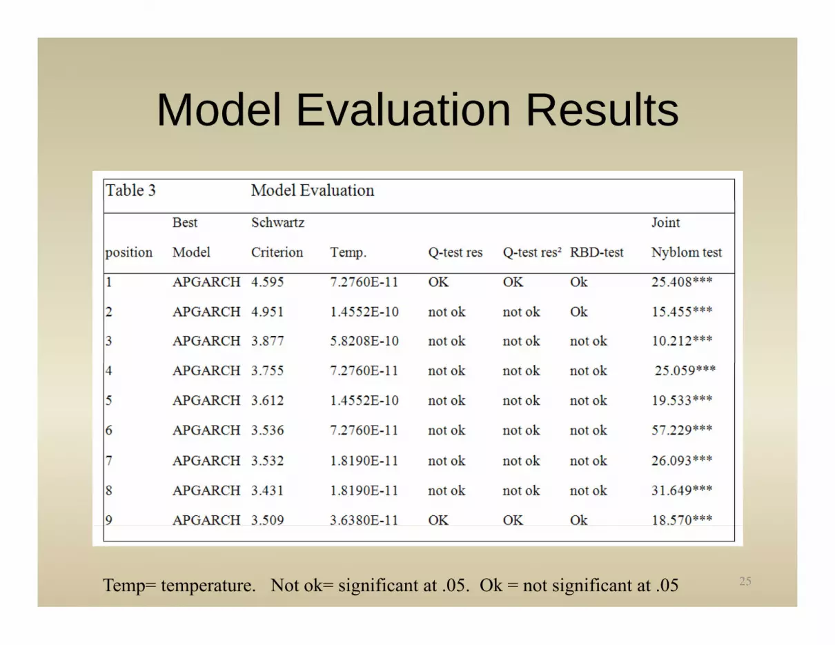
Model Evaluation ResultsModel Evaluation Results

25Temp= temperature. Not ok= significant at .05. Ok = not significant at .05

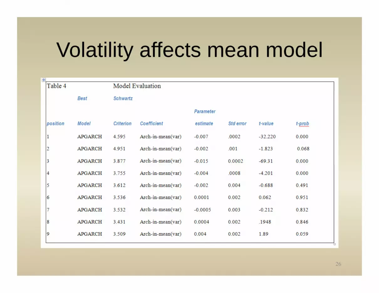
Volatility affects mean modelVolatility affects mean model

26

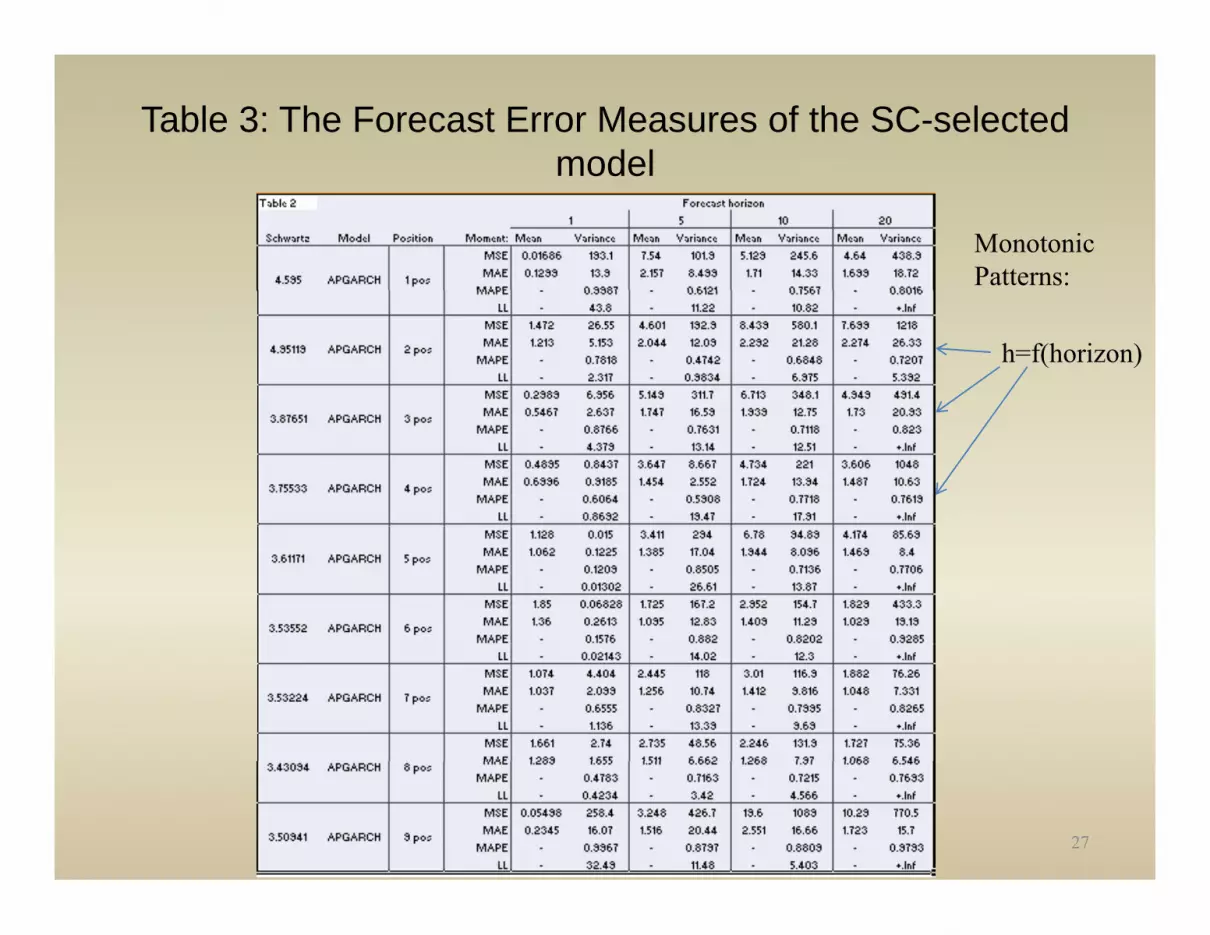
Table 3: The Forecast Error Measures of the SC-selected modelmodel

Monotonic Patterns:

h=f(horizon)

27

Model Selection by Forecast Error MMeasure

Table 4Preferred Variance Models

Forecast 1 5 10 20Error model value model value model value model value

Position Measure1 MSE Rmsa RMB 193.1 APG 101.9 Rmsa RMB 245.6 APG 438.9

MAE Rmsa RMB 13.9 APG 8.499 Rmsa RMB 14.33 APG 18.72MAPE Rmsa RMB 0.9987 APG 0.6121 Rmsa RMB 0.7567 APG 0.8016

2 MSE APG 26.55 APG 192.9 Rmsa RMB 580.1 Rmsa 1218

APG=APGARCHRMB= RiskMetrics

MAE APG 5.153 APG 12.09 Rmsa RMB 21.28 APG 26.33MAPE APG 0.7818 RMB 0.4742 Rmsa RMB 0.6848 APG 0.7207

3 MSE APG 6.956 Rmsa 311.7 APG 348.1 RMB 491.4MAE APG 2.637 RMsa 16.59 APG 12.75 APG 20.93MAPE APG 0.8766 RMsa 0.7631 APG 0.7118 APG 0.823

4 MSE APG 0.8437 APG 8.667 APG 221 APG 1048

BFGSRmsa= RiskMetrics

simulatedannealing

MAE APG 0.9185 APG 2.552 APG 13.94 APG 10.63MAPE APG 0.6064 APG 0.5908 APG 0.7718 APG 0.7619

5 MSE APG 0.015 APG 294 APG 94.89 APG 85.69MAE APG 0.1225 APG 17.04 APG 8.096 APG 8.4MAPE APG 0.1209 APG 0.8505 APG 0.7136 APG 0.7706

6 MSE APG 0.06828 APG 167.2 APG 154.7 APG 433.3

annealing

Possible RM preferenceMAE APG 0.2613 APG 12.83 APG 11.29 APG 19.19

MAPE APG 0.1576 APG 0.882 APG 0.8202 APG 0.9285

7 MSE APG 4.404 APG 118 APG 116.9 APG 76.26MAE APG 2.099 APG 10.74 APG 9.816 APG 7.331MAPE APG 0.6555 APG 0.8327 APG 0.7995 APG 0.8265

8 MSE APG 2.74 APG 48.56 APG 131.9 APG 75.36

preference on positions 1,2, or 3.

28

MAE APG 1.655 APG 6.662 APG 7.97 APG 6.546MAPE APG 0.4783 APG 0.7163 APG 0.7215 APG 0.7693

9 MSE APG 258.4 APG 426.7 APG 1089 APG 770.5MAE APG 16.07 APG 20.44 APG 16.66 APG 15.7MAPE APG 0.9967 APG 0.8797 APG 0.8809 APG 0.9793

Conclusions 1Conclusions 1

• Two models can model all nine positions ofTwo models can model all nine positions of UK natural gas futures: RiskMetrics GARCH and APGARCHand APGARCH.

• Two algorithms can work with RiskMetrics GARCH and one algorithm can work withGARCH and one algorithm can work with APGARCH to perform this task.

RM BFGS d i l t d li– RM: BFGS and simulated annealing– APGARCH: simulated annealing

29

Conclusions 2Conclusions 2

• The best models for all positions are theThe best models for all positions are the APGARCH with the simulated annealing algorithm according to the Schwartz criterionalgorithm, according to the Schwartz criterion, and passage of residual diagnostic assumptionsassumptions.

30

Conclusions 3Conclusions 3

• Only the first and nine position models pass allOnly the first and nine position models pass all of the residual diagnostics tests and the RBD testtest.

• However, none of the models passes the joint Nyblom Stability testNyblom Stability test.

31

Conclusions 4Conclusions 4

• Only the first 4 positions have volatilityOnly the first 4 positions have volatility models significantly negatively impacting the percentage log returns mean modelspercentage log returns mean models.

• Yet these impacts are small—generally less than 1 percent Contracts for large volumesthan 1 percent. Contracts for large volumes would be necessary to obtain substantial returns on these transactionsreturns on these transactions.

32

Conclusions 5Conclusions 5

• None of the models are stableNone of the models are stable.• This finding suggests that caution be exercised

in forecastingin forecasting. – Forecasting near horizons rather than far horizons

might be preferredmight be preferred.• Only on positions 2, 3, and 4 does the

l tilit i t i ll f tivolatility increase monotonically as a function of the forecast horizon.

33

Conclusions 6

• APGARCH generally outperform the other models in forecasting

• Evaluation is done by MSE, MAE, and MAPE• APGARCH is generally the optimal model—a useful bit of

knowledge for planners, risk managers, and traders in theknowledge for planners, risk managers, and traders in the UK gas futures market.– Only in the 1 day ahead and 10 day ahead does the RiskMetrics

outperform the APGARCH for position 1p p– For Position 2, RM outperforms 10 trading days out. – For Position 3, only 5 days out, does the RM simulated

annealing outperform the APGARCH.

34

Directions for Future ResearchDirections for Future Research1. Replication on more recent data could serve to p

confirm or disconfirm our findings.2. Boxing day trading anomaly for 2nd position 3. Exploring the asymmetry anomaly

1. No sign bias effect in most cases2 Significant gamma parameter in the APGARCH2. Significant gamma parameter in the APGARCH3. Leverage size versus leverage sign effects4. Volatility skew (change over positions)5. Volatility smile and smirk graphical analysis6. Power analysis for Sign Bias test.

35

Directions for Future Research 2Directions for Future Research 2

4 Do simulations for out-of-sample h step4. Do simulations for out-of-sample h step ahead VaR.

5 Replicate methods for analysis of other5. Replicate methods for analysis of other energy markets (electricity, oil, coal, etc.)

6 E l d i di i l l i6. Explore dynamic conditional correlation between the U.K. electricity and natural gas

kmarkets.

36

ReferencesReferences• Alexander, C., 2001. Market Models. Wiley, New York.• Brooks, C., and Persand, G., 2003. Volatility Forecasting for Risk Management, 22, 1-22.• Bollerslev, Tim, 1986, Generalized Autoregressive Conditional Heteroskedasticity, Journal of Econometrics, 31, 307-327.Bollerslev, Tim, 1986, Generalized Autoregressive Conditional Heteroskedasticity, Journal of Econometrics, 31, 307 327.• Ding, Z., Granger, C.W.J., and Engle, R.F. (1993). A Long-Memory Property of Stock Market Returns and a New Model. Journal of Empirical Finance, 1, 83-106.• Doornik, J. A. (2007). Ox 5: An Object Oriented Matrix Programming Language. Timberlake Consultants: London, U.K., 283.• Doung?(see page 4).• Engle, R. F. (1982) Autoregressive Conditional Heteroskedasticity with Estimates of Variance of United Kingdom inflation. In Granger, C. W. J. and Engle, R.F. (eds.) ARCH Selected

Readings, Oxford University Press, Chapter 1.• Engle, R.F. and Bollerslev, T. (1986). Modeling the Persistence of Conditional Variances. Economic Review, 5, 1-50.• Engle, R. F., Lilien, D.M. and Robins,R.P. (1987). Estimating the Time-Varying Risk Premia in the Term Structure: The ARCH-m model. Econometrica, 55/2, 391-407.• Engle, R.F. and Manganelli, S. (1999). CAViAR: Conditional Autoregressive Value at Risk by Regression Quantiles. University of California, San Diego working paper 99-20.• Energy Information Administration, Office of Oil and Gas, 2007. An analysis of Price Volatility in Natural Gas Markets, 1- 21.• Engle, R.F. and Bollerslev, T. (1986). Modelling the Persistence of Conditional Variances. Economic Review, 5, 1-50.• Ewing, Bradley T., Malik, F., and Ozfidan, O., 2002. Volatility Transmission in the Oil and Natural Gas Markets, Energy Economics, (24), 525-538.• Eydeland, A. And K. Woliniec, 2003, Energy and Power Risk Management: New Developments in Modeling, Pricing and Hedging, Wiley.• Garcia R.C., Contreras J., Van Akkeren M., and Garcia J. (2005), A GARCH Forecasting Model to Predict Day-Ahead Electricity Prices, Power Systems, IEEE transactions, IEEE

Transactions, 20(2), 867-874. • Geman H., 2005, Commodites and commodity derivatives – Modeling and Pricing for Agriculturals, Metals and Energy, Wiley.• Giot, P. and Laurent, S. (2003). Value-at-Risk for Long and Short Trading Positions. Journal of Applied Econometrics, 18, 654-655.• Gill, P.E., Murray, W., and Wright, M.H. (1981). Practical Optimization. San Diego: Academic Press, 137,160-161.• Giot, P. and Laurent, S. (2003). Value-at-Risk for Long and Short Trading Positions. Journal of Applied Econometrics, 18, 654-655.• Glosten, Lawrence R., Jagannathan, Ravi and Runkle, David E., 1993, On the Relation between the Expected Value and the Volatility of the Nominal Excess Returns on Stocks, Journal of

Finance, 48(5), 1779-1801.• Goffe, W.L., Ferrier, G.D., Rodgers, J. (1994). Global optimization of statistical functions with simulated annealing. Journal of Econometrics, Vol 60, Elsevier Science Publishers, North

Holland, pp. 65-99.• Greene, W. H. (2008) Econometric Analysis. Upper Saddle River, NJ: Pearson-Prentice Hall,1071. • ICE, 2007, ICE Futures U.K. Natural Gas Future Contract, April 20 2007 (found at www.theice.com)• Ilex 2004 Gas Prices in the U K Ilex Energy Consulting Report October 2004Ilex, 2004, Gas Prices in the U.K., Ilex Energy Consulting Report, October 2004.• Kupiec, P. (1995): “Techniques for Verifying the Accuracy of Risk Measurement Models,” Journal of Derivatives, 2, 173-84• Li C., and Zhang M., (2007), Application of GARCH Model in the Forecasting of Day-Ahead Electricity Prices, IEEE Computer Society.• Malo P., and Kanto A., (2005), Evaluating Multivariate GARCH Models in the Nordic Electricity Markets, Helsinki School of Economics Working paper, W-382. •

37

References-cont’dReferences cont d• Mauro, A., 1999, Price Risk Management in the Energy Industry: The Value at Risk Approach. Paper presented to the XXII Annual International

Conference of the International Association of Energy Economics, 9 – 12 June 1999, Rome.• Morgan J P (1996) RiskMetrics Technical Document 4th ed World Wide Web:http://hp idefi cnrs fr/bruno/enseignements/master2/RiskMetrics pdf• Morgan, J.P. (1996). RiskMetrics Technical Document 4th ed., World Wide Web:http://hp.idefi.cnrs.fr/bruno/enseignements/master2/RiskMetrics.pdf.• Mu, X., 2004, Weather, Storage, and Natural Gas Price Dynamics: Fundamentals and Volatility, Working Paper.• Laurent, S. (2007). Estimating and Forecasting ARCH models Using G@RCH. Timberlake Consulting, Ltd. London, U.K..• Laurent, S. (2008a). Personal e-mail communication regarding the distinction between the ESF measures, April 4, 2008.• Laurent, S. (2008b). Personal e-mail communication about the success rate, May 18, 2008.• Lopez, J. (1999) Evaluating the Predictive Accuracy of Volatility Models, FRB of San Francisco, p.6.• Nelson, Daniel B., 1991, Conditional Heteroscedasticity in Asset Returns: A New Approach, Econometrica, 59(2), 347-370., , , y pp , , ( ),• Pindyck, Robert S., 2004a. Volatility and Commodity Price Dynamics, Journal of Futures Markets, 24(11), 1029-1047.• Pindyck, Robert S., 2004b. Volatility in Natural Gas and Oil Markets, Journal of Energy and Development, 30(1), 1-19.• Poon, S. H. (2005). A Practical Guide to Forecasting Financial Volatility. Wiley: New York, 23-24.• Press, W.H., Teukolsky, S.A., Vertterling, W.T., and Flannery, B.P.(2007), Numerical Recipes: The Art of Scientific Computing, 3rd ed., New York:

Cambridge University Press, 521-522, 549-551.• Regnier, Eva, 2007. Oil and Energy Price Volatility, Energy Economics, 29, 405-427.• Sadorsky Perry 2006 Modelling and Forecasting Petroleum Futures Volatility Energy Economics 28 467 488• Sadorsky, Perry, 2006. Modelling and Forecasting Petroleum Futures Volatility, Energy Economics, 28, 467-488.• Serletis, A., and Shahmoradi, A., 2006. Returns and Volatility in the NYMEX Henry Hub Natural Gas Futures Market, OPEC Review, 171-186.• Simmons & Company, 2004, U.K. Natural Gas: Prices & Volatility Increasing, Oil Service Industry Research Report, March 11 2004.• Susmel, R., and Thompson, A., 1997, Volatility, Storage and Convenience: Evidence from Natural Gas Markets, Journal of Futures Markets, 17(1),

17-43. • Tsay, R.S. (2005). Analysis of Financial Time Series, 2nd ed. Wiley: New York, 97-153.• Wilson, B., Aggarwal, R., and Inclan C., 1996. Detecting Volatility Changes Across the Oil Sector, Journal of Futures Markets, 16(3), 313-330.• Worthington A.C., and Higgs H., (2003), A multivariate GARCH analysis of the domestic transmission of energy commodity prices and volatility: A

comparison of the peak and off-peak periods in the Australian electricity spot market, Discussion papers in economics, finance and international competitiveness.

• Wright, Philip, 2006, Gas Prices in the U.K.: Markets and Insecurity of Supply, Oxford Institute of Energy Studies.

38

Thank You!

We’ll be happy to entertain anyWe ll be happy to entertain anyquestions you might havenow.

39