how to incorporate volatility and risk in electricity price forecasting

May 2000

© 2000, Elsevier Science Inc., 1040-6190/00/$–see front matter PII S1040-6190(00)00102-0

65

How to Incorporate Volatility and Risk in Electricity Price Forecasting

Because traditional production-costing models do not represent the multi-commodity electricity market, ignore transmission constraints, and neglect volatility, they are unsuitable for evaluating the emerging competitive electricity markets. A better method of analysis is offered by models that simulate the volatility of the fundamental drivers causing electricity price swings with a Multi-Commodity Multi-Area Optimal Power Flow model.

Rajat Deb, Richard Albert, Lie-Long Hsue, and Nicholas Brown

n the competitive environment, investors, buyers and traders

not only need insight into prices, but also assessment of the risks of buying and selling electricity at the forecast prices. The key to risk management and option valua-tion is volatility. While the Black-Scholes and Black’s models are used successfully for option valua-tion in the securities, stock, and commodity markets, Black’s appli-cation to electricity prices does not predict volatility commensurate with the actual price risk. A more

accurate way to quantify electricity price risks over any period is by simulating the volatility of the fun-damental drivers with a structural model. Structural models excel—where traditional, single-product models’ utility ends—because of their internally consistent forecasts across energy, ancillary services, and imbalance markets.

This article presents an electricity price forecast and volatility analysis for 2000 using hourly Monte Carlo simulation of the California Power Exchange (PX) and Independent

Rajat Deb

is President of LCGConsulting, Los Altos, CA, and chiefarchitect of the UPLAN program. He

has built models for all phases of utilityplanning, including optimal generation

expansion, production costing,reliability evaluation, and financial

analysis. He holds a Ph.D. in systemsand information science and an S.M. in

Operations Research fromSyracuse University.

Rich Albert

is Vice President ofConsulting for LCG Consulting. Heserved as project director for LCG’s

study of the impact of restructuring inCalifornia. Prior to joining LCG, he

served as Principal Consultant for theWestern Region for Energy

Management Associates, Atlanta. Heholds an S.M. in engineering/economic

sciences from Stanford University.

Lie-Long Hsue

is LCG Consulting’sDirector of Software Development and

Support. She has extensivedevelopment experience in utility

demand, supply, and financialsimulations for investor-owned,

cooperative, municipal, and crown-corporation utilities in the United

States and abroad. She holds an S.M. incomputer science and an M.B.A. from

the University of California atSanta Clara.

Nicholas Brown

is an energy analystwith LCG Consulting and holds a B.A.in economics from Rutgers University.Substantial contributions were made to

this article by several others at LCG:Dr. Sachi Begur, Director ofConsulting; and Dr. Paresh

Rupanagunta, Ms. Julie Chien, and

Dr. Joydeep Mitra, Senior Consultants.

I

66


The Electricity Journal

System Operator (ISO). This study was performed with a structural model of the Western System Co-ordinating Council (WSCC), and based upon the statistical behavior of major variables, including load, hydro conditions, transmission interfaces’ simultaneous transfer capability, unit outages, and fuel prices. The Monte Carlo simulation method indicates the instanta-neous volatility, among various vol-atility measures, by forecasting hourly price distributions. We dem-onstrate that time-series models which impute future day-to-day volatility through a variant of Brownian motion with drift can produce significant errors in option valuation, even when relying on the aforementioned comprehen-sive price distributions. Rather, as we show in this article, direct com-putation of option values from such distributions provides superior ac-curacy in risk assessment.

I. Background

Prior to deregulation and the Federal Energy Regulatory Com-mission’s Order 888, forecasts of electricity prices were mainly used for ratemaking and analysis of qualified facilities, and were there-fore primarily focused on predict-ing the average and marginal costs of electricity. These forecasts were generally produced using single-commodity, production-costing models. In the emerging competi-tive environment, investors, buyers, and traders not only need insight into future electricity prices, but also assessment of the risks of buying and selling electric-

ity at the forecast prices. The choice of a forecast, especially a forecast upon which a risk man-agement strategy depends, must consider how completely the fore-cast represents and predicts risk.

II. Competition Requires a New Approach

In a competitive electricity mar-ket, the spot or day-ahead prices are not determined purely on a

casting requires a multi-commodity, multi-area model capable of vola-tility simulation.

1

A. Risk Assessment Is a Necessary Component of Forecasting

In addition to price forecasts, what kinds of information are nec-essary for managing risk? The call and put option values at the fore-cast price are valuable sources of information, which represent the buyers’ and sellers’ risks associ-ated with a particular forecast. The key to option valuation and risk management is volatility, which refers to the swiftness with which a price changes, and often signifies a transition from one price regime to another. The electricity markets are known for high short-term vol-atility relative to that observed in the markets for more traditional commodities.

B. Why Traditional Methods are Inappropriate

One method of options valuation, based on the Black-Scholes or Black’s models, relies on historical projections of the day-to-day vola-tility. While this method, based on Black’s model in particular, has been successfully used for option valuation in many commodity mar-kets, the application of Black’s model to electricity prices as if elec-tricity were a standard commodity does not provide predictions about volatility commensurate with the actual price risk. Some of the short-comings of multiple-factor volatil-ity analysis using historical projec-tions are cited below.

•

The electric system is subject

Traditional production-costing models do not

represent the multi-commodity electricitymarket, ignore trans-mission constraints,

and neglect volatility.

cost basis. Rather, they are based on the market participants’ ratio-nal competitive behavior, and their objective of maximizing income from all available markets, includ-ing the ancillary service and emis-sion allowance markets. The tradi-tional production-costing models do not represent the multi-commodity electricity market, ignore transmission constraints, and neglect volatility; these mod-els are therefore unsuitable for the emerging competitive electricity markets in today’s environment. It has become apparent that in a mar-ket like California, accurate fore-

May 2000


67

to the confluence of unusually high demand, unexpected genera-tor outages, and transmission de-ratings.

•

Instantaneous demand and supply imbalances subject the sys-tem to unusual stress; this can only be captured by hourly volatility, not by day-to-day volatility.

•

Ancillary services (A/S), emis-sion allowances (EA), and other products interact with energy prices and cannot be treated as iso-lated entities. Black’s model is not suited for cross-market analysis, especially in California, New York, New England, and Ontario, where such markets exist.

•

Past conditions are unlikely to be repeated in any consistent man-ner useful in forecasting.

We will provide empirical evi-dence of how the results of volatil-ity analysis using historical time series of prices can be misleading, with the California Power Exchange (PX) as the focus of study.

We believe that by far the supe-rior way to obtain accurate mea-sures of electricity price risks over any period of time is by simulating the volatility of the fundamental drivers causing the electricity price swings with a Multi-Commodity Multi-Area Optimal Power Flow Model (MMOPF). Felak, writing about ideal software for traders, emphasizes the need for such models and asserts that “chrono-logical, security-constrained analy-sis of least-cost commitment and dispatch, with full AC optimal power-flow representation” alone can provide “location-specific spot prices.”

2

We will use a forecast of the 1998

and 1999 California PX prices, con-ducted for the California Energy Commission by our firm, LCG Con-sulting, in 1996,

3

followed by a fore-cast of year 2000 PX prices and its volatility to make our point. The purpose of the 1996 forecast was to evaluate restructuring proposals for the California market prior to the enactment of California restructur-ing legislation. Readers may also be interested in a recent paper by Earle

et al.

on the

III. Role of Volatility in Electricity Prices and Risk Assessment

In most commodity markets, the price effects of production or supply-chain problems are damp-ened by surplus storage. By con-trast, most electricity systems lack storage for all practical purposes. The electricity market therefore experiences pronounced short-term volatility due to the need for continuous balancing of demand and supply. Volatility in the elec-tricity market is rooted in hourly, daily, and seasonal uncertainty associated with fundamental mar-ket drivers and the physics of gen-eration and delivery of electricity. A sudden heat wave can strain the ability of even backup generator capacity to meet elevated demand in a timely manner. The generators are subject to unexpected outages and changing emission con-straints, while transmission lines may experience congestion, creat-ing electrical imbalances.

When the actual value of any driver departs from what is used in a simulation, electricity prices can deviate significantly from the forecast. A point forecast based purely on the most likely, or expected, values of the drivers therefore gives only the most prob-able outcome for each hour. Such a forecast represents one sample path out of myriad potential sample paths.

The variability of the underlying drivers and the physical character-istics of the electricity market are the primary reasons for short-term volatility unknown in conven-

When the actual value of any driver departs from what is used in a simulation, electricity prices can deviate significantly from

the forecast.

California experience, covering 1998 and 1999.

4

Our overriding concern in this article is the analysis and use of volatility, and how to incorporate risk through appropriate modeling of the underlying process.

his will also permit compari-son of both the original and

new methods’ results with the actual market outcomes of 1998 and 1999. In time, the year 2000 forecast results can be compared with the actual prices of the entire current year. An analysis of the option values associated with the volatility is provided as part of this discussion.

T

68



tional commodity markets. Since the values of many fundamental drivers are highly uncertain over the long term, an approach to elec-tricity price forecasts based on single-point estimates of drivers is neither sufficient for determining market participants’ day-to-day strategy nor suitable for asset valu-ation.

5

Thus, a more comprehen-sive forecast must capture the con-sequences of random and atypical fluctuations of fundamental mar-ket drivers and must be based on an accurate representation of the electrical system.

IV. Volatility Measures and Recent California Experience

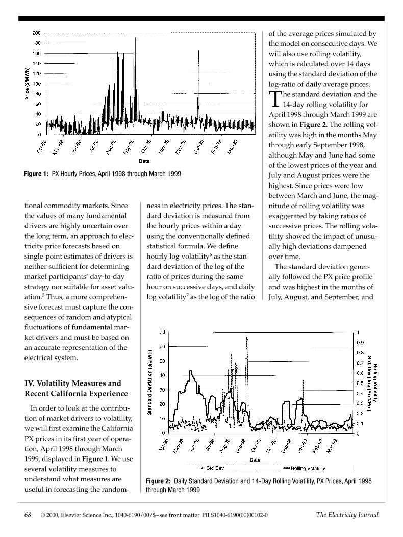
In order to look at the contribu-tion of market drivers to volatility, we will first examine the California PX prices in its first year of opera-tion, April 1998 through March 1999, displayed in

Figure 1

. We use several volatility measures to understand what measures are useful in forecasting the random-

ness in electricity prices. The stan-dard deviation is measured from the hourly prices within a day using the conventionally defined statistical formula. We define hourly log volatility

6

as the stan-dard deviation of the log of the ratio of prices during the same hour on successive days, and daily log volatility

7

as the log of the ratio

of the average prices simulated by the model on consecutive days. We will also use rolling volatility, which is calculated over 14 days using the standard deviation of the log-ratio of daily average prices.

he standard deviation and the 14-day rolling volatility for

April 1998 through March 1999 are shown in

Figure 2

. The rolling vol-atility was high in the months May through early September 1998, although May and June had some of the lowest prices of the year and July and August prices were the highest. Since prices were low between March and June, the mag-nitude of rolling volatility was exaggerated by taking ratios of successive prices. The rolling vola-tility showed the impact of unusu-ally high deviations dampened over time.

The standard deviation gener-ally followed the PX price profile and was highest in the months of July, August, and September, and

Figure 1: PX Hourly Prices, April 1998 through March 1999

Figure 2: Daily Standard Deviation and 14-Day Rolling Volatility, PX Prices, April 1998 through March 1999

T

May 2000


69

low during April through June. In July through September, recurring fluctuations in load caused expen-sive generators to be taken on- and off-line frequently. This contrib-uted to high price variations, and consequently, high volatility in both measures. The volatility mea-sures were lower in the remaining months, through March 1999.

These results indicate that rolling volatility does not discriminate between high and low prices. For example, if the price increases from $0.50 to $10 during off-peak time and from $80 to $1,600 during on-peak hours, the log-ratio treats the increases as having contributed the same volatility. It appears that the standard deviation is an intu-itively appealing measure of the variability in price. For instance, readers can translate one standard deviation above the mean as includ-ing prices that will be exceeded only 16 percent of the time.

V. 1996 PX Study for CEC

LCG Consulting’s proprietary structural model, UPLAN,

8

was used to forecast California electric-ity prices and to simulate the par-ticipants’ behavior in the energy and ancillary markets. UPLAN is a Multi-Commodity, Multi-Area Optimal Power Flow (MMOPF) model with the ability to simulate volatility using Monte Carlo simu-lation. The model integrates the market participants and their rationally competitive bidding behavior, generation assets, the transmission network, and its flow restrictions across interfaces. Each price driver is represented either in

the bidding and scheduling sub-model, or in the real-time OPF model. The program not only incorporates the energy and ancil-lary service markets, but also the interaction of energy prices with ancillary service prices, as well as the emissions allowance market. The result of this multi-commodity simulation is an internally consis-tent forecast of prices across mar-kets. Thus, the MMOPF-type model’s ability to represent the

are essentially consistent with past and expected conditions in the real world. The 1996 forecast was aimed at determining the most likely prices, predicated on a set of expected values of major variables or drivers.

A. Input Variables in 1996 PX Forecast

The California study was based on data developed by the Califor-nia Energy Commission (CEC), the California Public Utility Commis-sion, and the utilities in California (CFM 10). The data were cross-checked with the 1995 Load and Resources Report and the Path Rating Catalogue prepared by the Western System Coordinating Council, or WSCC (DOE Form OE-411).

9

The hydrological conditions were based on a normal water year, as projected by the WSCC. Prices of natural gas and other fuels were derived from the CEC’s biennial fuel price projection.

10

The demand forecast was developed from data provided by each of the individual utilities within California, while the loads outside California were based on WSCC projections. All of these fundamental drivers were treated as single-point variables on a monthly basis and no provisions were made about any variability of these fundamental drivers.

B. 1998–1999 PX Actuals’ Impact on Prices

The input assumptions for the price forecast for 1998 turned out to be remarkably true in many regards, except for the hydrologi-cal conditions and the forecasted summer loads. This caused the

The input assumptions for the price forecast for 1998 turned out to be remarkably true

in many regards.

physical resources with specificity, and to achieve an hourly balance of demand and supply resources, sets it apart from any other form of modeling and provides unequaled accuracy in forecasting prices. In addition, such a model can be used for consistent analysis of volatility and thus account for the large, unforeseen discrepancies that often occur between the forward and spot prices of electricity across time.

s has been discussed, a certain amount of variation in the

conditions surrounding any mar-ket is anticipated. Nonetheless, a forecast must rely on inputs that

A

70



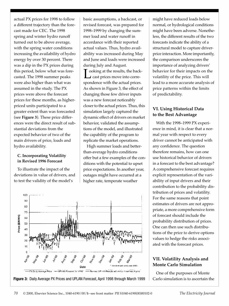
actual PX prices for 1998 to follow a different trajectory than the fore-cast made for CEC. The 1998 spring and winter hydro runoff turned out to be above average, with the spring water conditions increasing the availability of hydro energy by over 30 percent. There was a dip in the PX prices during this period, below what was fore-casted. The 1998 summer peaks were also higher than what was assumed in the study. The PX prices were above the forecast prices for these months, as higher-priced units participated to a greater extent than was forecasted (see

Figure 3

). These price differ-ences were the direct result of sub-stantial deviations from the expected behavior of two of the main drivers of price, loads and hydro availability.

C. Incorporating Volatility in Revised 1996 Forecast

To illustrate the impact of the deviations in value of drivers, and to test the validity of the model’s

basic assumptions, a backcast, or revised forecast, was prepared for 1998–1999 by changing the sum-mer load and water runoff in accordance with their reported actual values. Thus, hydro avail-ability was increased during May and June and loads were increased during July and August.

ooking at the results, the back-cast prices move into corre-

spondence with the actual prices. As shown in Figure 3, the effect of changing those few driver inputs was a new forecast noticeably closer to the actual prices. Thus, this simulation largely captured the dynamic effect of drivers on market behavior, validated the assump-tions of the model, and illustrated the capability of the program to replicate the market operations.

High summer loads and better-than-average hydro conditions offer but a few examples of the con-ditions with the potential to upset price expectations. In another year, outages might have occurred at a higher rate, temperate weather

might have reduced loads below normal, or hydrological conditions might have been adverse. Nonethe-less, the different results of the two forecasts indicate the ability of a structural model to capture driver-price interaction. More importantly, the comparison underscores the importance of analyzing drivers’ behavior for their impacts on the volatility of the price. This will lead to a more accurate analysis of price patterns within the limits of predictability.

VI. Using Historical Data to the Best Advantage

With the 1998–1999 PX experi-ence in mind, it is clear that a nor-mal year with respect to every driver cannot be anticipated with any confidence. The question therefore remains, how can one use historical behavior of drivers in a forecast to the best advantage? A comprehensive forecast requires explicit representation of the vari-ability of input drivers and their contribution to the probability dis-tribution of prices and volatility. For the same reasons that point estimates of drivers are not appro-priate, a more comprehensive form of forecast should include the probability distribution of prices. One can then use such distribu-tions of the price to derive options values to hedge the risks associ-ated with the forecast prices.

VII. Volatility Analysis and Monte Carlo Simulation

One of the purposes of Monte Carlo simulation is to ascertain the Figure 3: Daily Average PX Prices and UPLAN Forecast, April 1998 through March 1999

L

May 2000


71

systematic effect of market drivers upon price variability. When a structural model of the type used in this study generates a large number of Monte Carlo simula-tions of the system, it captures physical or instantaneous volatil-ity as well as the temporal varia-tion in price levels. We compare the volatility of the year 2000 fore-cast with the actual volatility of the PX prices from April 1998 through the latter part of 1999. The success of the model in cap-turing driver-price causality can be judged on the basis of the rela-tive magnitude of the volatility observed throughout the year.

A. Forecast of PX Prices and Risk Assessment for 2000

For the year 2000 forecast and volatility analysis, a series of 100 Monte Carlo simulations were per-formed to determine the distribu-tion of PX prices. Preparations for the volatility analysis involved the determination of probability distri-butions of the input variables,

using historical values of these variables. Samples were drawn from four input variables, namely Loads, Hydro Availability, Fuel Prices, and Transmission conges-tion. All relevant markets, includ-ing the PX energy, A/S, and the real-time imbalance market, were modeled.

The simulations performed by the model provided daily distribu-

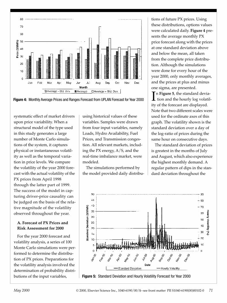
tions of future PX prices. Using these distributions, options values were calculated daily.

Figure 4

pre-sents the average monthly PX price forecast along with the prices at one standard deviation above and below the mean, all taken from the complete price distribu-tion. Although the simulations were done for every hour of the year 2000, only monthly averages, and the prices at plus and minus one sigma, are presented.

n

Figure 5

, the standard devia-tion and the hourly log volatil-

ity of the forecast are displayed. Note that two different scales were used for the ordinate axes of this graph. The volatility shown is the standard deviation over a day of the log-ratio of prices during the same hour on consecutive days.

The standard deviation of prices is greatest in the months of July and August, which also experience the highest monthly demand. A regular pattern of dips in the stan-dard deviation throughout the

Figure 4: Monthly Average Prices and Ranges Forecast from UPLAN Forecast for Year 2000

Figure 5: Standard Deviation and Hourly Volatility Forecast for Year 2000

I

72



year denotes the weekends, when load is normally lower and prices remain low relative to what is seen on weekdays. On the same days, during the changeover, the hourly log volatility displays spikes.

B. Comparison of Historical Volatility in the PX Market and in the 2000 Forecast

In

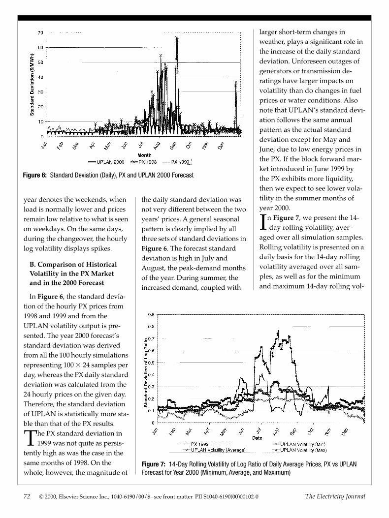
Figure 6

, the standard devia-tion of the hourly PX prices from 1998 and 1999 and from the UPLAN volatility output is pre-sented. The year 2000 forecast’s standard deviation was derived from all the 100 hourly simulations representing 100

3

24 samples per day, whereas the PX daily standard deviation was calculated from the 24 hourly prices on the given day. Therefore, the standard deviation of UPLAN is statistically more sta-ble than that of the PX results.

he PX standard deviation in 1999 was not quite as persis-

tently high as was the case in the same months of 1998. On the whole, however, the magnitude of

the daily standard deviation was not very different between the two years’ prices. A general seasonal pattern is clearly implied by all three sets of standard deviations in

Figure 6

. The forecast standard deviation is high in July and August, the peak-demand months of the year. During summer, the increased demand, coupled with

larger short-term changes in weather, plays a significant role in the increase of the daily standard deviation. Unforeseen outages of generators or transmission de-ratings have larger impacts on volatility than do changes in fuel prices or water conditions. Also note that UPLAN’s standard devi-ation follows the same annual pattern as the actual standard deviation except for May and June, due to low energy prices in the PX. If the block forward mar-ket introduced in June 1999 by the PX exhibits more liquidity, then we expect to see lower vola-tility in the summer months of year 2000.

n

Figure 7

, we present the 14-day rolling volatility, aver-

aged over all simulation samples. Rolling volatility is presented on a daily basis for the 14-day rolling volatility averaged over all sam-ples, as well as for the minimum and maximum 14-day rolling vol-

Figure 6: Standard Deviation (Daily), PX and UPLAN 2000 Forecast

Figure 7: 14-Day Rolling Volatility of Log Ratio of Daily Average Prices, PX vs UPLAN Forecast for Year 2000 (Minimum, Average, and Maximum)

T

I

May 2000


73

atility observed over all the sam-ples for each day. We conclude that the simulated average volatil-ity is consistent with the rolling volatility of 1999 PX prices. We will now turn to the evaluation of risk implied in the volatility of the forecast for the year 2000.

VIII. Risk and Options Valuation

The key to options pricing for a commodity is the estimation of the spread between the forward price and the spot price. As mentioned, one of the well-known methods for options pricing of standard com-modities is Black’s model. It has been applied of late to evaluate options for electricity transactions as well. Black’s model requires one to impute the volatility of the price from the historical data using some variant of Brownian motion with drift. Based on the computed vola-tility, options prices are deduced.

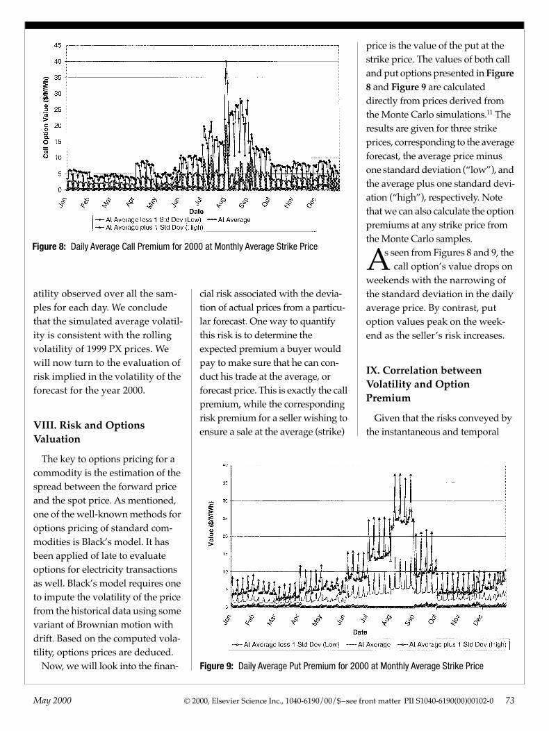
Now, we will look into the finan-

price is the value of the put at the strike price. The values of both call and put options presented in

Figure 8

and

Figure 9

are calculated directly from prices derived from the Monte Carlo simulations.

11

The results are given for three strike prices, corresponding to the average forecast, the average price minus one standard deviation (“low”), and the average plus one standard devi-ation (“high”), respectively. Note that we can also calculate the option premiums at any strike price from the Monte Carlo samples.

s seen from Figures 8 and 9, the call option’s value drops on

weekends with the narrowing of the standard deviation in the daily average price. By contrast, put option values peak on the week-end as the seller’s risk increases.

IX. Correlation between Volatility and Option Premium

Given that the risks conveyed by the instantaneous and temporal

cial risk associated with the devia-tion of actual prices from a particu-lar forecast. One way to quantify this risk is to determine the expected premium a buyer would pay to make sure that he can con-duct his trade at the average, or forecast price. This is exactly the call premium, while the corresponding risk premium for a seller wishing to ensure a sale at the average (strike)

Figure 8: Daily Average Call Premium for 2000 at Monthly Average Strike Price

Figure 9: Daily Average Put Premium for 2000 at Monthly Average Strike Price

A

74



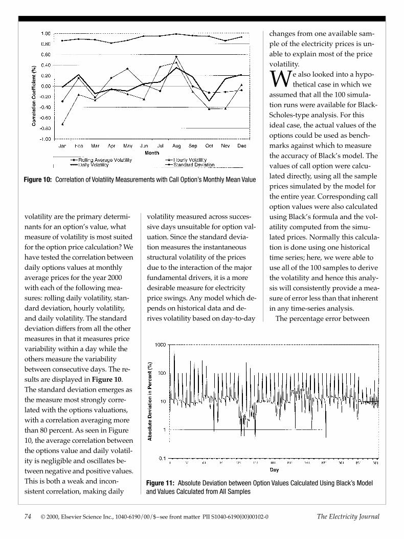
volatility are the primary determi-nants for an option’s value, what measure of volatility is most suited for the option price calculation? We have tested the correlation between daily options values at monthly average prices for the year 2000 with each of the following mea-sures: rolling daily volatility, stan-dard deviation, hourly volatility, and daily volatility. The standard deviation differs from all the other measures in that it measures price variability within a day while the others measure the variability between consecutive days. The re-sults are displayed in

Figure 10

. The standard deviation emerges as the measure most strongly corre-lated with the options valuations, with a correlation averaging more than 80 percent. As seen in Figure 10, the average correlation between the options value and daily volatil-ity is negligible and oscillates be-tween negative and positive values. This is both a weak and incon-sistent correlation, making daily

volatility measured across succes-sive days unsuitable for option val-uation. Since the standard devia-tion measures the instantaneous structural volatility of the prices due to the interaction of the major fundamental drivers, it is a more desirable measure for electricity price swings. Any model which de-pends on historical data and de-rives volatility based on day-to-day

changes from one available sam-ple of the electricity prices is un-able to explain most of the price volatility.

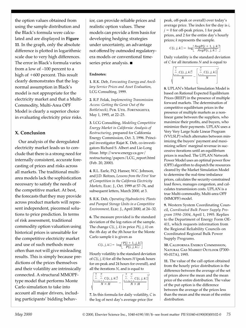
e also looked into a hypo-thetical case in which we

assumed that all the 100 simula-tion runs were available for Black-Scholes-type analysis. For this ideal case, the actual values of the options could be used as bench-marks against which to measure the accuracy of Black’s model. The values of call option were calcu-lated directly, using all the sample prices simulated by the model for the entire year. Corresponding call option values were also calculated using Black’s formula and the vol-atility computed from the simu-lated prices. Normally this calcula-tion is done using one historical time series; here, we were able to use all of the 100 samples to derive the volatility and hence this analy-sis will consistently provide a mea-sure of error less than that inherent in any time-series analysis.

The percentage error between

Figure 10: Correlation of Volatility Measurements with Call Option’s Monthly Mean Value

Figure 11: Absolute Deviation between Option Values Calculated Using Black’s Model and Values Calculated from All Samples

W

May 2000


75

the option values obtained from using the sample distribution and the Black’s formula were calcu-lated and are displayed in

Figure 11

. In the graph, only the absolute difference is plotted in logarithmic scale due to very high differences. The error in Black’s formula varies from a low of –100 percent to a high of

1

600 percent. This result clearly demonstrates that the log-normal assumption in Black’s model is not appropriate for the electricity market and that a Multi-Commodity, Multi-Area OPF Model is clearly a superior choice in evaluating electricity price risks.

X. Conclusion

Our analysis of the deregulated electricity market leads us to con-clude that there is a strong need for internally consistent, accurate fore-casting of prices and risks across all markets. The traditional multi-area models lack the sophistication necessary to satisfy the needs of the competitive market. At best, the forecasts that they may provide across product markets will repre-sent independent, piecemeal solu-tions to price prediction. In terms of risk assessment, traditional commodity option valuation using historical prices is unsuitable for the competitive electricity market and use of such methods more often than not will give misleading results. This is simply because pre-dictions of the prices themselves and their volatility are intrinsically connected. A structural MMOPF-type model that performs Monte Carlo simulation to take into account all major drivers, includ-ing participants’ bidding behav-

ior, can provide reliable prices and realistic option values. These models can provide a firm basis for developing hedging strategies under uncertainty, an advantage not offered by outmoded regulatory-era models or conventional time-series price analysis.

j

Endnotes:

1.

R.K. Deb,

Forecasting Energy and Ancil-lary Service Prices and Asset Evaluation

, LCG Consulting, 1999.

2.

R.P. Felak,

Implementing Transmission Access: Getting the Genie Out of the Bottle(neck)

,

Pub. Util. Fortnightly

, May 1, 1995, at 22–25.

3.

LCG Consulting,

Modeling Competitive Energy Market in California: Analysis of Restructuring, prepared for California Energy Commission, Oct. 3, 1996. Princi-pal investigator Rajat K. Deb, co-investi-gators Richard S. Albert and Lie-Long Hsue. http://www.energy.ca.gov/restructuring/papers/LCG_report.html (Feb. 20, 2000).

4. R.L. Earle, P.Q. Hanser, W.C. Johnson, and J.D. Reitzes, Lessons from the First Year of Competition in the California Electricity Markets, Elec. J., Oct. 1999 at 57–76, and subsequent letters, March 2000, at 3.

5. R.K. Deb, Operating Hydroelectric Plants and Pumped Storage Units in a Competitive Environment, Elec. J., April 2000, at 24–32.

6. The measure provided is the standard deviation of the log-ratios of the sample. The change C(i, j, k) in price P(i, j, k) on the ith day at the jth hour for the Monte Carlo sample k is given as

Hourly volatility is the standard deviation of C(i, j, k) for all the hours H (peak hours for on-peak and 24 hours for overall), and all the iterations N, and is equal to

7. In this formula for daily volatility, C is the log of next day’s average price (for

C i j k, ,( ) logP i 1 j k, ,1( )

P i j k, ,( )--------------------------------5

C i j k, ,( )2

j 15

H

^k 15

N

^

N H3-------------------------------------------

C i j k, ,( )j 15

H

^k 15

N

^

N H3-----------------------------------------

2

2

peak, off-peak or overall) over today’s average price. The index for the day is i, j 5 0 for off-peak prices, 1 for peak prices, and 2 for the entire day’s hourly prices; k represents the sample.

Daily volatility is the standard deviation of C for all iterations N and is equal to

8. UPLAN’s Market Simulation Model is based on Rational Expected Equilibrium Prices (REEP) in the presence of multiple forward markets. The determination of competitive equilibrium prices in the presence of multiple markets as a non-linear game between the suppliers, who maximize their profits, and buyers, who minimize their payments. UPLAN uses a Very Very Large Scale Linear Program (VVLSLP) which alternates between min-imizing the buyers’ payment and maxi-mizing sellers’ marginal revenue in suc-cessive iterations until an equilibrium prices is reached. The UPLAN Network Power Model uses an optimal power flow (OPF) algorithm to dispatch the resources cleared by the Market Simulation Model to determine the real-time imbalance prices, calculates the security-constrained load flows, manages congestion, and cal-culates transmission costs. UPLAN is a true Multi-commodity, Multi-area OPF (MMOPF) model.

9. Western System Coordinating Coun-cil, Coordinated Bulk Power Supply Pro-gram 1994–2004, April 1, 1995. Replies to the Department of Energy Form OE-411, which requests information from the Regional Reliability Councils on Coordinated Regional Bulk Power Supply Programs.

10. California Energy Commission, Natural Gas Market Outlook (P300-95-017A), 1995.

11. The value of the call option obtained from the hourly price distribution is the difference between the average of the set of prices above the mean and the mean price of the entire distribution. The value of the put option is the difference between the average of the prices less than the mean and the mean of the entire distribution.

C i j k, ,( ) logAvgP i 1 j k, ,1( )

AvgP i j k, ,( )-------------------------------------------5

C i j k, ,( )2

k 15

N

^

N----------------------------------

C i j k, ,( )k 15

N

^

N--------------------------------

2

2

how to incorporate volatility and risk in electricity price forecasting

Documents