volatility modeling and forecasting for banking stock returns
TRANSCRIPT
Volatility Modeling and Forecasting for Banking Stock Returns
Krishna Murari*
sector have improved the health of the banking sector. The reforms recently introduced include the enactment of the Securitization Act to step up loan recoveries, establishment of asset reconstruction companies, initiatives on improving recoveries from non-performing assets (NPAs) and change in the basis of income recognition. These reforms have raised transparency and efficiency in the banking system. Spurt in treasury income and improvement in loan recoveries have helped Indian banks to record better profitability. The effect of all such changes has been crucial on the stock prices of the banks. Besides the above, there are large variations in the information content of the bank stock price, measured by the extent to which bank stocks synchronize with the whole markets. The bank stock price movements are more aligned with the whole market and suggest that the bank stock returns are less influenced by bank-specific information (Roll, 1988).
Volatility is a measure of variability in the price of an asset. Volatility is associated with unpredictability and uncertainty about the price. It is often used as synonymous of risk which means higher the volatility, higher the risk in the market (Kumar & Gupta, 2009). In other words, we can say that the stock market incorporates information, then high volatility arises out of diversified information inputs or less confirmed information which leads to disruption of market. As a concept, volatility is simple and intuitive. It measures variability or dispersion about a central tendency. To be more meaningful, it is a measure of how far the current price of an asset deviates from its average past prices. Greater the deviation, greater is the volatility. At a more fundamental level, volatility can indicate the strength or conviction behind a price move (Raju, 2004). It is difficult to estimate about the future trend of volatility in market because it is affected
* Assistant Professor, Department of Commerce, Mody Institute of Technology & Science, Sikar, Rajasthan, India. Email: [email protected]
Abstract
In this paper, an attempt has been made to model and forecast the short term volatility of the Indian banking sector. A popular banking sector CNX bank index of national stock exchange of India (NSE) which includes 12 most liquid and large capitalized Indian banking stocks is used as a time series. Data have been collected since the inception of the index i.e. January 2000; a total of 3122 observations up to the period of June 2013, are used in modeling the volatility of the banking stock returns using univariate Box-Jenkins or ARIMA model. ADF test and unit root testing is done to know the stationarity of the series, later the AR(p) and MA(q) orders are identified with the help of minimum information criterion as suggested by Hannan- Rissanen. As per the analysis, ARIMA (1,0,2) model was found to be the best fit to forecast the volatility of bank stock returns. The final equation for the model is which can be helpful to the investors and speculators in taking their short run buying and selling decisions for bank stocks.
Keyword: CNX Bank Index, Bank Stock Returns, Stationarity, Volatility, ARIMA Modeling, ForecastingJEL Codes: Classification: G17
Introduction
The Indian banking industry has witnessed key changes, dazzling a number of underlying developments since 2000. Innovation in communication and information technology has facilitated growth in internet banking, ATM network, electronic transfer of funds, and quick diffusion of information. Structural reforms in the banking
Article can be accessed online at http://www.publishingindia.com
18 International Journal of Banking, Risk and Insurance Volume 1 Issue 2 September 2013
by a large number of factors including political stability, economic fundamentals, government budget, policies of the government, corporate performance etc. However, by calculating historical volatility a prediction can be assumed about the future trend in the volatility.
Modeling and forecasting volatility of a daily financial asset price return is an important and challenging financial problem that has received a lot of attention in recent days. The decision of the investors to sell or to buy depend directly on the volatility of securities prices that they expect to happen in the near future, since they build their predictions on the movements of the securities prices whether up or down, that is to protect themselves from the losses that they may meet, or to reduce it as much as possible. The purpose of this study is to model the volatility of returns on Indian banking sector using univariate Box-Jenkins (ARIMA) model, furthermore, forecast volatility and identify lags to achieve this goal.
Univariate Box-Jenkins (UBJ) or Autoregressive Integrated Moving Average (ARIMA) models are especially suited to short-term forecasting. Pankratz (1983) considered short-term forecasting, because most ARIMA models place heavy emphasis on the recent past rather than the distant past. This emphasis on the recent past means, that long-term forecasts from ARIMA models are less reliable than short-term forecasts.
Charles A. et al. (2008) studied the relationship between stock markets and foreign exchange market, and determined whether movements in exchange rates have an effect on stock market in Ghana. They found that depreciation in the local currency leads to an increase in stock market returns in the long run whereas in the short run it reduces stock market returns. Mohammad S. et al. (2009) modeled the relationship between macroeconomic variables and prices of shares in Karachi stock exchange in Pakistan from 1986 to 2008 period. They showed that internal factors of firms like increase in production and capital formation do not affect significantly while external factors like exchange rate and reserve are in effects. Siti R. et al. (2011) analyzed the crude oil prices using Box-Jenkins methodology and Generalized Autoregressive Conditional Heteroscedasticity, they found that ARIMA (1,2,1) and GARCH(1,1) are the appropriate models under model identification, estimation, diagnostic checking and forecasting future prices. Samnel (2011) used ARIMA model to predict inflation in Ghana, they
found that inflation is integrated of order one and follows (6,1,6) order.
Al-Zeaud and Ali (2011) fitted the ARIMA (2,0,2) model for weekly date of banks sector from Amman Stock Exchange (ASE) for a period of 2005 to 2010. Kaur (2004) investigated the nature and characteristics of stock market volatility in India with emphasis on ‘day of the week effect’ or the ‘weekend effect’ using volatility cluster modeling. She found that asymmetrical GARCH models outperform the conventional OLS models and symmetrical GARCH models by the application of asymmetrical GARCH models EGARCH (1,1) to Sensex and TARCH (1,1) to Nifty returns. Sohail C. et al. (2012) identified and estimated the mean and variance components of the daily closing share price using ARIMA-GARCH type models by explaining the volatility structure of the residuals obtained under the best suited mean models for the time series. Many other works have also been carried out in order to identify the stock return behaviour and time series volatility modeling in various countries (Abdalla & Suliman, 2012); (Poon & Granger, 1992); (Ocran & N., 2007); (Gokcan, 2000); (Bollerslev, 1976); (Faisal, 2012); (Alberg, Shalit, & Yosel, 2008); (Kumar S. S., 2006); (Tripathy, 2010).
This paper investigates the nature and characteristics of banking stock returns volatility in India. The objective of the study is to model the volatility of banking stock returns in Indian stock market through UBJ analysis or the ARIMA modeling. The checking of the validity of the fitted model is done through the residual analysis, normality of residuals and residuals versus fitted line of the time series.
Research DesignDatabase and Period of Study
In order to have a good benchmark of the Indian banking sector, India Index Service and Product Limited (IISL) developed the CNX Bank Index. The daily stock price data on CNX Bank Index have been taken from Datazone, the online database of NSE. The database contains all the actively traded stocks from banking sector at any given time on the NSE. CNX Bank Index is an index comprised of the most liquid and large capitalized Indian banking stocks. It provides investors and market intermediaries with a benchmark that captures the capital market
Volatility Modeling and Forecasting for Banking Stock Returns 19
performance of Indian banks. The index has 12 stocks from the banking sector which trade on the National Stock Exchange.
The CNX Bank Index represents about 14.44% of the free float market capitalization of the stocks listed on NSE and 85.50% of the free float market capitalization of the stocks forming part of the banking sector universe as on March 30, 2012 (NSE, 2012). The study spans the period January 2000 (with base value of 1000) through June 2012.
Daily stock prices have been converted to daily returns. The present study uses the logarithmic difference of prices of two successive periods for the calculation of rate of return. The logarithmic difference is symmetric between up and down movements and is expressed in percentage terms for ease of comparability with the straightforward idea of a percentage change.
If Pt be the closing level of Index on date t and Pt-1 be the same for its previous business day, i.e., omitting intervening weekend or stock exchange holidays, then the one day return on the market portfolio is calculated as:
Yt = LNpP
t
t-
ÊËÁ
ˆ¯̃
¥1
100
where, LN(z) is the natural logarithm of ‘z.’
Statistical Tools
The daily stock price data have been first processed by using Microsoft Excel. Subsequently, time series analysis packages EViews and MINITAB programs have been used to test the banking index dynamics, return and volatility data for various statistical properties and to estimate ARMA and ARIMA class of models.
Econometric Methodology
In any time series analysis, the test for stationarity is important because, in the presence of non-stationary series, the standard estimation procedures are not applicable. Thus, we begin our analysis with testing for stationarity, i.e., unit root testing. We then fit an ARMA model to the data generating process and follow the process suggested by Box and Jenkins (1976).
Testing of Stationarity of the Time Series
Unit Root Testing
A test of stationarity (or non-stationarity) that has been widely popular over the past several years is the unit root test. We start with Yt = rYt–1 + mt; –1£ r £ 1 (1)
where, mt is a white noise error term.Now, subtracting Yt –1 from both sides of the above equation Yt – Yt –1 = rYt–1 – Yt–1 + mt;
DYt = (r – 1)(Yt–1) + mt
DYt = d Yt–1 + m1 (2)
where 1δ ρ= − and ∆ is the first difference operator. In practice, to test the null hypothesis that 0δ = . If 0δ = then ρ =1 that is, there is a unit root, meaning thereby the time series is non-stationary.
Augmented Dickey Fuller Test
Yt in equation (1) is assumed that the error term tµ was uncorrelated. But, in case tµ is correlated, Dickey and Fuller developed a test known as the Augmented Dickey-Fuller (ADF) test. This test is conducted by augmenting the preceding equation by adding the lagged values of the dependent variable tY∆ . To be specific, the ADF test here consists of estimating the following regression
1
1
m
t t i t i ti
Y Y Yδ α ε− −=
∆ = + ∆ +� (3)
where tε is pure white noise error term and the no. of lagged difference terms so that the error term in equation (3) is serially uncorrelated.
AR, MA and ARIMA Modeling of Banking Stock Returns
An Autoregressive (AR) Process
Let Yt represents the daily bank stock return at time t. If we model Yt as (Yt – δ) = a1 (Yt–1 – δ ) + ut
20 International Journal of Banking, Risk and Insurance Volume 1 Issue 2 September 2013
where δ is the mean of Y and ut is and uncorrelated random error term with zero mean and constant variance s 2 (i.e. white noise), then we say that Yt follows a first order autoregression, or AR (1) stochastic process.
Yt can be modeled for pth order autoregressive or AR (p) process as
1 1 2 2( ) ( ) ( ) ...... ( )t t t p t p tY Y Y Y uδ α δ α δ α δ− − −− = − + − + − +
1 1 2 2( ) ( ) ( ) ...... ( )t t t p t p tY Y Y Y uδ α δ α δ α δ− − −− = − + − + − + (4)
A Moving Average (MA) Process
Suppose we model Y as Bank Index as follows
0 1 1t t tY u uµ β β −= + +
where µ a constant and u is a white noise stochastic error term. Here, Y at time t is equal to a constant plus a moving average of the current and past error terms. Thus, the above equation follows a first order moving average or MA (1) process.
To generalize, moving average or MA(q) process can be written as
0 1 1 2 2 ....t t t t q t qY u u u uµ β β β β− − −= + + + + (5)
An Autoregressive and Moving Average (ARMA) Process
It is quite likely that Y has characteristics of both AR and MA and is therefore ARMA. Thus, if Yt follows an ARMA(1, 1) process can be written as
1 1 0 1 1t t t tY Y u uθ α β β− −= + + + ; (6)
where q represents a constant term.
An ARIMA Modeling Process
Generally, many of the time series which are not stationary are integrated. Therefore, if we have to difference a time series d times to make it stationary and them apply ARMA (p, q) model to it, we say that original time series is ARIMA (p, d, q) that is an autoregressive Integrated Moving Average time series where p denotes the no. of autoregressive terms, d the no. times the series has to be differenced before it becomes stationary and q the no.
of moving average terms (Gujrati, 2003). The ARIMA modeling process consists of following steps: 1. SpecificationofARIMAOrdersHannan- Rissanen (Hannan & Rissanen, 1982) procedure is used to specify the autoregressive and moving average orders of an ARIMA model. It is assumed that the order of differencing, d, and the deterministic terms have been pre-specified. The information criterions are often used as a guide in model selection. Following information criteria are used to identify the orders of ARIMA.Akaike Information Criterion AIC (n.l) =
log ( , ) ( )s 2 2 n lTn l+ + (7)
Schwarz Information Criterion SIC (n.l) =
log ( , ) log ( )s2 2 n l T
Tn l+ + (8)
Hannan-Quinn Information Criterion HQ(n.l) =
log ( , ) log(log ) ( )s 2 2 n l TT
n l+ + (9)
where s is the residual from fitted model from all combinations (n, l) for which n, l £ pmax < h. l is the value of the log of the likelihood function with the n parameters estimated using T observations. As a user of these information criteria for a model selection guide, the model with the smallest information criterion is selected. 2. EstimationAt this stage, we get precise estimates of the coefficients of the model chosen at the identification stage. We fit this model to the available data series to get estimates of ai, bj and q. This stage provides some warning signals about the adequacy of our model. In particular, if the estimated coefficients do not satisfy certain mathematical inequality conditions, that model is rejected. 3. Model Checking
Box and Jenkins (1976) suggest some diagnostic checks to determine whether an estimated model is statistically adequate? Checking of the adequacy of an ARIMA model is done with the help of residual autocorrelation and non-normality test. TestforResidualAutocorrelationThe portmanteau test is used to check the following pair of hypotheses
Volatility Modeling and Forecasting for Banking Stock Returns 21
H0 : ru,1 = º = ru, h = 0
versus H1 : ru,i π 0 f or at least one i = 1, º , h,
where ru, i = Corr (ut, ut – i ) denotes the autocorrelation coefficient of the residual series. If the ut are residuals from an estimated ARMA (p,q) model, the portmanteau test statistics is
Qh = T jh
u j=Â 12r ,
(10)
where r su j t jT
tst j
sts
t uT u u and u u, /= =-= + -Â1 1� � � � � are the
standardized estimation residuals.
Jarque-Bera Test for Non-Normality
This test is based on the third and fourth moments of a distribution i.e. skewness and kurtosis. Denoting the standardized estimation residuals by , the test checks whether the third and fourth moments of the standardized residuals are consistent with a standard normal distribution. The test statistics is
JB = T T u T T utT
ts
tT
ts
6 2431
13 2 1
14 2[ ( ) ] [ ( ) ]-
=-
=+ -ÂÂ (11)
where T utT
ts-
=Â1 13( ) is a measure for the skewness of
the distribution and tT
tsu=Â 14( ) for the kurtosis. The
test statistic has an asymptotic x2 (2) distribution if the null hypothesis is correct and the null hypothesis is rejected if JB is large.
ARCH-LMTestThe test for neglected autoregressive conditional heteroskedasticity (ARCH) is done based on an ARCH (q) model to the estimation residuals,
u u u et t q t q t� � � �2
0 1 12 2
= + + +- -b b b (12)
Checking the null hypothesis H0 : b1 = = bq = 0 versus H1 : b1 π 0 or bq π 0.
Under the normality assumptions the LM statistics is obtained from the coefficient of determination, R2 of regression of above equation. ARCHLM(q) = TR2 (13)
It has an asymptotic χ2 (q) distribution if the null hypothesis of no conditional heteroskedasticity holds (Engle, 1982).
4. Forecasting Under Univariate Box-Jenkins (UBJ) analysis or ARIMA Model building for volatility, the last step is to forecast the asset returns with a specification of lower and upper bound. This step includes the prediction of the financial asset returns using the model so developed on the basis of ARIMA (p,d,q) orders.
Empirical Findings and Analysis of Banking Sector VolatilityDiagnostic Tests
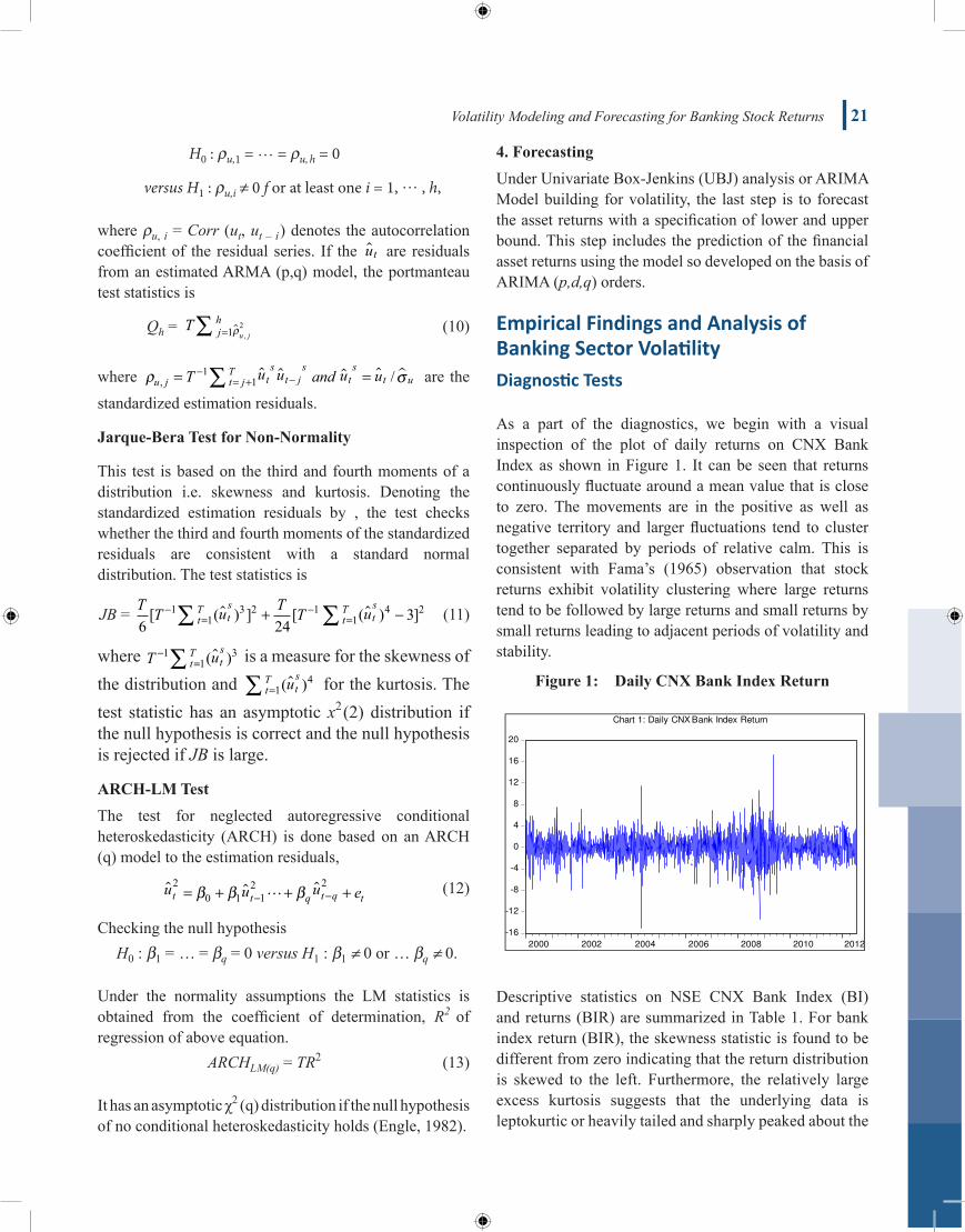
As a part of the diagnostics, we begin with a visual inspection of the plot of daily returns on CNX Bank Index as shown in Figure 1. It can be seen that returns continuously fluctuate around a mean value that is close to zero. The movements are in the positive as well as negative territory and larger fluctuations tend to cluster together separated by periods of relative calm. This is consistent with Fama’s (1965) observation that stock returns exhibit volatility clustering where large returns tend to be followed by large returns and small returns by small returns leading to adjacent periods of volatility and stability.
Figure1: DailyCNXBankIndexReturn
-16
-12
-8
-4
0
4
8
12
16
20
2000 2002 2004 2006 2008 2010 2012
Chart 1: Daily CNX Bank Index Return
Descriptive statistics on NSE CNX Bank Index (BI) and returns (BIR) are summarized in Table 1. For bank index return (BIR), the skewness statistic is found to be different from zero indicating that the return distribution is skewed to the left. Furthermore, the relatively large excess kurtosis suggests that the underlying data is leptokurtic or heavily tailed and sharply peaked about the
22 International Journal of Banking, Risk and Insurance Volume 1 Issue 2 September 2013
mean when compared with the normal distribution. The Jarque-Bera statistic calculated to test the null hypothesis of normality rejects the normality assumption. The results confirm the well-known fact that daily banking index returns are not normally distributed but are leptokurtic and skewed.
Table 1: Descriptive Statistics
Statistics Bank Index close(BI)Natural log returns
(BIR)
Study Period January 2000 to June 2012
Observations 3123 3122
Mean 4935.274 0.074826
Median 4315.750 0.086346
Maximum 13268.70 17.23940
Minimum 743.7000 -15.13805
Std. Dev. 3527.746 2.102930
Skewness 0.473230 -0.175904
Kurtosis 1.902359 7.953452
Jarque-Bera 3207.914
Probability 0.000
Sum 233.6083
Sum Sq. Dev. 13802.05
Testing of Stationarity
The non-stationary time series could produce a weak result. To avoid the spurious correlation problem, it is
essential to test for unit root of the index employed in the study. A unit root test determines whether a time series variable is non-stationary using an autoregressive model. In this study the augmented Dickey- Fuller test is used to test the existence of a unit root as the null hypothesis.
Table 2 showed the ADF test for stock indices for bank-ing sector. The results of this workout strongly confirms that at the standard 5% significance level the bank indices return series is stationary in levels, so there is no need to use any transformation on the time series BIR and BKXR.
Table 2: UnitRootTestingofBIR
NullHypothesis:BIRhasaunitroot
Exogenous: Constant Lag Length: 0 (Automatic - based on SIC, maxlag=28) t-Statistic Prob.*
Augmented Dickey-Fuller test statistic -49.3049 0.0001Test critical values: 1% level -3.43226 5% level -2.86227 10% level -2.5672
Identification of Arma Orders
The ARIMA (1,0,2) model has been identified using the information criterion. As a user of these information criteria for a model selection guide, the model with the smallest information criterion (AIC) is selected.
Table 3: OptimalLagSelectionforARIMAModeling
OPTIMAL LAGS FROM HANNAN-RISSANEN MODEL SELECTION
original variable: BIRorder of differencing (d): 0adjusted sample range: [01/01/2000 (5), 06/30/2012 (5)], T = 3122
optimal lags p, q (searched all combinations where max (p,q) <= 3)Akaike Info Criterion: p = 1, q = 2Hannan-Quinn Criterion: p = 2, q = 0Schwarz Criterion: p = 0, q = 1
Volatility Modeling and Forecasting for Banking Stock Returns 23
Estimation
Estimation of ARIMA models is done by Gaussian maximum likelihood (ML) assuming normal errors. The optimization of the likelihood function requires in general nonlinear optimization algorithms and here the algorithm by Ansely is used (Ansely, 1979). The maximization routine forces the AR coefficients to be invertible. The MA roots will have modulus 1 or greater. If an MA root is 1, the estimation routine will report a missing value for the MA coefficient’s standard deviation, t-statistic and p-value. An MA root equal to 1 suggests that d may have been chosen too large.
The estimates of the constant and the coefficients of the equation are obtained by employing least squares algorithms through a combination of search routines and successive approximations to obtain final least square point estimates of the parameters. The final estimates are those that minimize the sum of squared errors to a point where no other estimates can be found that yield smaller sum of squared errors. This is known as convergence. The
estimation output shows the number of iterations needed for convergence. It also shows some other statistics and the parameter estimates with standard errors, t-statistics and tail probabilities.
Thus, the final equation for the stationary time series for the bank stock return volatility is defined as:
Yt = 0.09314169 + 0.67310852Yt–1
+ 0.543357176ut–1 + 0.12303398u t–2 (14)
Since, the t-values for the coefficients MA(1) is insignificant, it can be dropped from the model, therefore equation becomes as follows:Yt = 0.09314169 + 0.67310852Yt–1 + 0.12303398ut–2
(15)
Model Checking
The portmanteau test statistics for residual autocorrelation tests whether any of a group of autocorrelations of the residual time series is different from zero. Looking at the tabular statistics, we conclude that the null hypothesis of
Table 4: ARIMA(1,0,2)ModelEstimates
Final Results:Iterations Until Convergence: 25Log Likelihood: -6720.461631 Number of Residuals: 3122 AIC : 13450.923262 Error Variance : 4.344656186SBC : 13481.154407 Standard Error : 2.084383886
DF: 3117 Adj. SSE: 13542.396131831 SSE: 13542.293330887
Dependent Variable: BIR Coefficients Std. Errors T-Ratio Approx. Prob.
AR1 0.67310852 0.21384738 3.14761 0.00166MA1 0.54357176 0.21296640 2.55238 0.01075MA2 0.12303398 0.02631811 4.67488 0.00000
CONST 0.09314169 0.07613016 1.22345 0.22125TREND -0.00001175 0.00004223 -0.27820 0.78087
Table 5: Test Statistics for Model Checking
Portmanteau Test Jarque Bera Test ARCH-LM TEST with 4 lags:
Test statistics 27.5827 test statistic: 2928.0025 test statistic: 293.7108 p-Value ( χ2 ): 0.0064 p-Value(χ2): 0.0000 p-Value(χ2): 0.0000Ljung and Box: 27.6745 skewness: -0.1324 F statistic: 81.0638 p-Value (Chi^2): 0.0062 kurtosis: 7.7369 p-Value(F): 0.0000
24 International Journal of Banking, Risk and Insurance Volume 1 Issue 2 September 2013
white noise residuals is accepted, thus we have a decent model.
Jarque-Bera test statistics for residuals also confirms that the third and fourth moments of the standardized residuals are consistent with a standard normal distribution. The p-value of 0.000 indicates that there is a 0.0% chance that we would have obtained our estimates of the parameters if the true parameters were zero. Since the p-value is small (less than the usually chosen a-level of 0.05) the ARCH-LM test is significant; thus we reject Ho hypothesis and conclude that there is no conditional heteroskedasticity in residuals.
Furthermore, Table 6 showed the correlation matrix of the estimated parameters, the strongest correlation was found between a2 and b1 but the smallest correlation is between a3 and b2. The correlation matrix for estimated parameters provides a means for recognizing the existence of parameter redundancy. Although the estimates of the parameters of Box-Jenkins model always have some correlation. Very high correlations (r >=0.8 or 0.9) between the estimates suggest parameter redundancy. When redundancy exists, a model of lower order should be fitted to the data. As seen in Table 6, the correlation matrix for the parameters there is no high correlation except one.
Table 6: CorrelationMatrixoftheEstimatedParameters
1 2 3 4
1 1.0002 0.996 1.0003 0.715 0.674 1.0004 -0.001 -0.001 -0.001 1.000
Before forecasting with the final equation, it is necessary to perform various diagnostic tests in order to validate the goodness of fit of the model. A good way to check the adequacy of a Box-Jenkins model is to analyze the residuals ( )Y Yt t- - 1 . If the residuals are truly random, the autocorrelations and partial autocorrelations calculated using the residuals should be statistically equal to zero. If they are not, this is an indication that we have not fitted the correct model to the data.
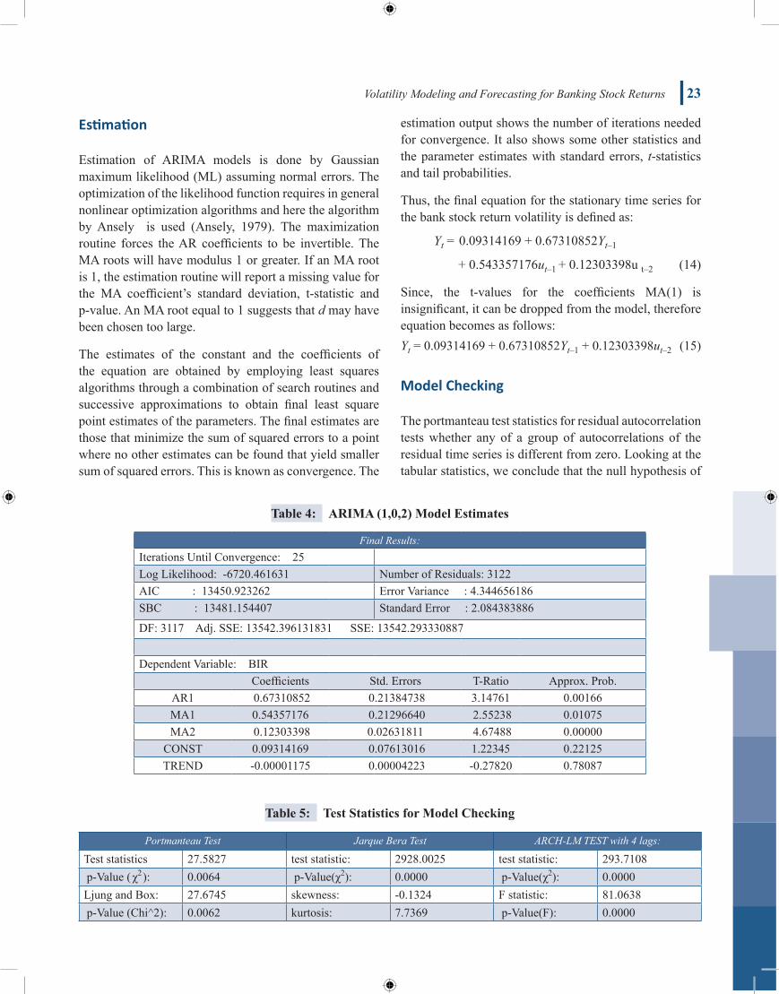
Chart, shown in Figure 2 known as the four-in-one residual plot, displayed four different residual plots together in one graph window. This layout can be useful
for comparing the plots to determine whether the model meets the assumptions of the analysis.
Figure2: ResidualPlotsforBIR
The normal probability plot indicated whether the residuals are normally distributed, other variables are influencing the response, or outliers exist in the data. And, the fit regression line showed how the residuals are closed to the fit line. The histogram indicated that whether the data are skewed or outliers exist in the data, the histogram showed approximately the whole data centered on the mean of data.
The residuals versus fitted values indicated whether the variance is constant, a nonlinear relationship exists. The last graph showed the residuals versus order observations for Banks sector volatility.
Forecasting
At the final stage, which is forecasting, once the fitted model has been selected, it can be used to generate forecasts for future time periods for the Banks volatility sector. Although, Minitab program and most other Box-Jenkins computer programs compute the forecasts and confidence intervals for the user, the final model for the volatility banks sector is illustrated in equation 15.
Table 7 showed the predicted 30 days ahead of the Bank returns volatility. Since, the whole data are 3122 observations (daily observation), so it is appropriate to choose the predicted value ahead for 30 observations, because ARIMA model adequate for the short term forecasts. While, chart in Figure 3 showed the plot of the actual and predicted values for the volatility banks sector,
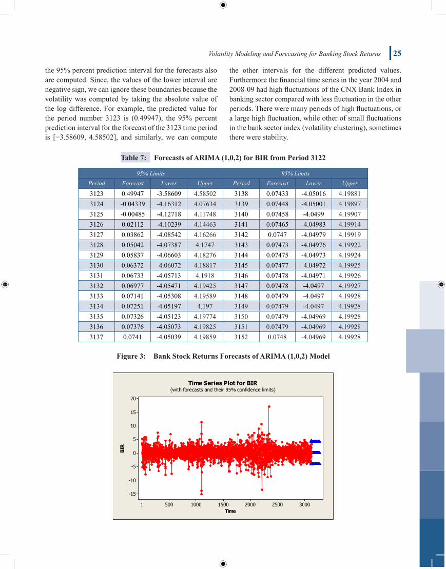
Volatility Modeling and Forecasting for Banking Stock Returns 25
the 95% percent prediction interval for the forecasts also are computed. Since, the values of the lower interval are negative sign, we can ignore these boundaries because the volatility was computed by taking the absolute value of the log difference. For example, the predicted value for the period number 3123 is (0.49947), the 95% percent prediction interval for the forecast of the 3123 time period is [−3.58609, 4.58502], and similarly, we can compute
the other intervals for the different predicted values. Furthermore the financial time series in the year 2004 and 2008-09 had high fluctuations of the CNX Bank Index in banking sector compared with less fluctuation in the other periods. There were many periods of high fluctuations, or a large high fluctuation, while other of small fluctuations in the bank sector index (volatility clustering), sometimes there were stability.
Table 7: ForecastsofARIMA(1,0,2)forBIRfromPeriod3122
95% Limits 95% LimitsPeriod Forecast Lower Upper Period Forecast Lower Upper
3123 0.49947 -3.58609 4.58502 3138 0.07433 -4.05016 4.198813124 -0.04339 -4.16312 4.07634 3139 0.07448 -4.05001 4.198973125 -0.00485 -4.12718 4.11748 3140 0.07458 -4.0499 4.199073126 0.02112 -4.10239 4.14463 3141 0.07465 -4.04983 4.199143127 0.03862 -4.08542 4.16266 3142 0.0747 -4.04979 4.199193128 0.05042 -4.07387 4.1747 3143 0.07473 -4.04976 4.199223129 0.05837 -4.06603 4.18276 3144 0.07475 -4.04973 4.199243130 0.06372 -4.06072 4.18817 3145 0.07477 -4.04972 4.199253131 0.06733 -4.05713 4.1918 3146 0.07478 -4.04971 4.199263132 0.06977 -4.05471 4.19425 3147 0.07478 -4.0497 4.199273133 0.07141 -4.05308 4.19589 3148 0.07479 -4.0497 4.199283134 0.07251 -4.05197 4.197 3149 0.07479 -4.0497 4.199283135 0.07326 -4.05123 4.19774 3150 0.07479 -4.04969 4.199283136 0.07376 -4.05073 4.19825 3151 0.07479 -4.04969 4.199283137 0.0741 -4.05039 4.19859 3152 0.0748 -4.04969 4.19928
Figure3: BankStockReturnsForecastsofARIMA(1,0,2)Model
26 International Journal of Banking, Risk and Insurance Volume 1 Issue 2 September 2013
Conclusion
The main aim of this study is to predict the short term volatility for banking sector stock returns using the best suited model for the purpose i.e. Autoregressive Integrated Moving Average (ARIMA) models. The data is obtained for daily (5 days) CNX bank index close from the website of NSE using the historical indices in the period from1/1/2000-6/30/2012. The plot of all volatility showed the structural breaks in the financial time series in the year 2004 and 2008-09 with high fluctuations as compared to less fluctuation in the other periods and there were many periods of a large high fluctuation, while other of small fluctuations in the bank stock returns (volatility clustering). The impact of such fluctuations in long past period was ignored because ARIMA modeling for short term forecasting emphasizes on the recent past rather than the distant past. In testing whether the financial time series of banks sector at 5% level are stationary at level (or differences) or not, we had concluded that the stationarity exists for banking sector at level.
In this study the best ARIMA model is chosen using the lowest information criterion (among AIC, SIC and HQ). The convenient model that fitted the data for the banking sector is ARIMA (1,0,2), at 95% confidence interval. The final forecasting model ARIMA (1,0,2) for bank stock return volatility is-
The above equation could be helpful to the investors in predicting the short term volatility for bank stocks for supporting their buying or selling decisions.
References
Abdalla, S. & Suliman, Z. (2012). Modelling Stock Returns Volatility: Empirical Evidence from Saudi Stock Exchange. International Research Journal of Finance and Economics, 85, 166-179.
Alberg, D., Shalit, H. & Yosel, R. (2008). Estimating stock market volatility using asymmetric GARCH models. Applied Financial Economics , 18, 1201-1208.
Al-Zeaud, & Ali, H. (2011). Modelling and Forecasitng volatility using ARIMA Model. European Journal of Economics, Finance and Administrative Sciences, (35), 109-126.
Ansely, C. (1979). An algorithm for the exact likelihood of a mixed autoregressive-moving average process. Biometrika, 66, 59-65.
Bollerslev, T. (1976). Generalized autoregressive condi-tional Heteroscedasticity. Journal of Econometrics, 31, 307-327.
Box, G. P. & Jenkins, G. (1976). Time Series Analysis, Forecasting and Control. San Francisco: Holden Day.
Charles, A., Simon, K. & Daniel, A. (2008). Effect of Exchange Rate Volatility on Ghana Stock Exchange. African Journal of Accounting, Economic, Finance and Banking Research, 3(3).
Faisal, F. (2012). Forecasting Bangladesh’s Inflation Using Time Series ARIMA Models. World Review of Business Research, 2(3), 100-117.
Fama, E. (1965). The behaviour of stock market prices. Journal of Business, 38(1), 34-105.
Gokcan, S. (2000). Forecasting Volatility of Emerging Stock Markets: Linear various Nonilnear GARCH models. Journal of Forecasting, 19, 499-504.
Gujrati, D. N. (2003). Basic Econometrics (4th ed.). New Delhi: Tata McGraw Hill.
Hannan, E. J. & Rissanen, P. (1982). Recursive estima-tion of mixed atoregressive-moving average order. Biometrika , 69, 81-94.
Kaur, H. (2004). Time Varying Volatility of the Indian Stock Market. Vikalpa, 29(4), 25-42.
Kumar, R. & Gupta, H. (2009). Volatility in Indian Stock Market: A Case of Individual Securities. Journal of Academic Research in Economics, 1(1), 43-54.
Kumar, S. S. (2006). Forecasting Volatility – Evidence from Indian Stock and Forex Markets. IIM Working Paper series, 6.
Mohammad, S., Hussain, A. & Ali, A. (2009). Impact of Macroeconomic Variable on Stock Prices: Empirical Evidence in case of KSE. European Journal of Scientific Research, 38(1).
NSE. (2012). Products: CNX Bank Index. Retrieved March 2012, from nseindia website: http://www.nseindia.com/products/content/equities/indices/sec-toral_indices.htm
Ocran, M. & N., B. (2007). Forecasting Volatility in Sub-Saharan Africa’s Commodity markets. Investment Management and Financial Innovations, 4(2), 91-102.
Pankratz, A. (1983). Forecasting with Univariate Box-Jenkins Models. New York: Hon Wiley & sons.
Poon, S. H. & Granger, C. (1992). Stock Returns and Volatility: An Empirical Study of the UK Stock Market. Journal of Banking and Finance, 16(1), 37-59.
Volatility Modeling and Forecasting for Banking Stock Returns 27
Raju, M. T. (2004). Stock Market Volatility – An International Comparison. Securities and Exchange Board of India . Working Paper Series No. 8.
Roll, R. (1988). R2. Journal of Finance, 43(3), 541-566.Samnel, E. A. (2011). ARIMA (autoregressive integrated
moving average)approach to predicating inflation in Ghana. journal of economics and international finance, 3(5), 328-326.
Siti, R., Maizah, H., Leechee, N. & Nokjant, M. (2011). Comparative Study on Box-Jenkins and GARCH models in forecasting crude Oil Prices. Journal of Applied Sciences, 11(7), 1129-1133.
Sohail, C., Kamal, S. & Ali, I. (2012). Modeling and Volatilty Analysis of share Prices using ARCH & GARCH Models. World Applied Science Journal, 19 (1), 77-82.
Torben, D. & Doberv, D. a. (2009). Jump-Robust Volatilty Estimation using Nearest Neighbor Truncation. working Paper. 15533.
Tripathy, N. (2010). The Empirical Relationship between Trading Volumes & Stock Return Volatility in Indian Stock Market. European Journal of Economics, Finance and Administrative Sciences, (24), 59-77.