short-term market efficiency in the futures markets: topix futures and 10-year jgb futures
TRANSCRIPT

Global Finance Journal 16 (2006) 330–353
Short-term market efficiency in the futures markets:
TOPIX futures and 10-year JGB futures
Joel Rentzler a, Kishore Tandon b,*, Susana Yu c
a Department of Economics and Finance, City University of New York-Baruch College, USAb Department of Economics and Finance, City University of New York-Baruch College, USA
c Department of Finance, Business Economics and Legal Studies, Iona College, USA
Received 1 October 2004; received in revised form 1 May 2005; accepted 1 October 2005
Available online 20 March 2006
Abstract
This paper examines the effect of the past price information on the two major futures contracts traded
on the Tokyo Stock Exchange: the TOPIX futures and the 10-year JGB futures. The unique 90-min lunch
break on the exchange creates twomini-sessions in each calendar-trading day. This paper compares these
contracts between the morning and afternoon sessions. In addition, percentage-returns and tick-size-
returns are used to measure the intraday price movements following past price performance. These
futures contracts present evidence of short-term market inefficiency over the period 1994 to 2003.
D 2006 Elsevier Inc. All rights reserved.
JEL classification: G14
Keywords: Index futures; Overreaction; Market efficiency
1. Introduction
As high-frequency trading data has become more accessible and computing technology
more affordable, researchers can now test the random hypothesis on a daily or intraday
basis. In addition, with the availability of intraday data, market imperfections such as bid–
ask spreads, commissions, and market impact, can be handled with more accuracy when
testing for market inefficiencies. The objective of this paper is to examine the short-term
1044-0283/$ -
doi:10.1016/j.g
* Correspond
York, One Be
E-mail add
see front matter D 2006 Elsevier Inc. All rights reserved.
fj.2006.01.006
ing author. Zicklin School of Business, Box B10-225, Baruch College City University of New
rnard Baruch Way, New York, NY 10010, USA. Tel.: +1 646 312 3468.
ress: [email protected] (K. Tandon).

J. Rentzler et al. / Global Finance Journal 16 (2006) 330–353 331
efficiency in the two futures contracts traded on the Tokyo Stock Exchange (TSE).
Persistent price movements, either continuance or reversal, following past price
information is construed as proof of a lack of short-term efficiency on the TSE.
There is a growing interest in testing the short-term efficiency of futures markets. Tse
(1999) examines the Japanese government bond (JGB) futures, listed on both the London
and the Tokyo futures exchanges, and concludes that both markets are equally efficient.
Lee, Gleason, and Mathur (2000) examine the French futures exchange and validate the
random walk hypothesis. Fung, Mok, and Lam (2000) provide strong support for the
intraday overreaction theory in the Hong Kong futures market but only minor support in
the U. S. futures market. In addition, Fung and Lam (2004) show the existence of intraday
overreaction during intraday trading and market closing on Hang Seng Index futures
contracts. They suggest that pricing error of the index futures relative to its fair value can
be used to identify investors’ overreaction in index futures markets. Grant, Wolf, and Yu
(2005) test the short-term efficiency of the U.S. equity index futures market examining 15
years of intraday data and conclude that the market may be inefficient for very short
horizons. However, bid–ask spreads and market impact may seriously dampen the
potential profit of a strategy designed to exploit this short-term inefficiency. Researching
seven major currency futures contracts traded on the Chicago Mercantile Exchange,
Rentzler, Tandon, and Yu (in press) conclude that large daily or opening price moves can
be used to predict immediate intraday price movement patterns.
This paper differs from others in several ways. First, the TSE has a morning session and
an afternoon session separated by a 90-min lunch break, which creates a gap in the
information flow and generates two pairs of opening and closing prices within a calendar-
trading day. Second, this study uses an adaptive filter rule to alleviate the bias caused by
choosing an arbitrary filter, which may commit a fallacy of prophecy. Third, this study
adopts two measures of price movements, percentage movements and tick-size movements,
to evaluate results from trading futures contracts. Although the first measure is widely
recognized, the second measure allows for a clearer interpretation and is also more suitable
for futures trading where there is an investment base problem. Finally, this study examines
the robustness of pricing errors across two sub-periods to check if these short-term
inefficiencies persist.
The remainder of this paper is organized as follows. Section 2 describes the TSE, the
TOPIX and 10-year JGB futures contracts, data characteristics, and two measures of past
price performances in each session. Section 3 presents the methodology, which includes
regression analysis, the adaptive filter rule and day-of-the-week analysis. The fourth
section reports the empirical results of the four filters (measures) over the 1994 to 2003
period. Section 5 concludes the findings of the paper.
2. Data
The Tokyo Stock Price Index (TOPIX) is a market-value-weighted composite index of
all common stocks listed on the First Section of the Tokyo Stock Exchange (TSE).1 The
1 The TSE domestic stock market is divided into two sections – the First and Second Sections. The First Section
is the market place for stocks of larger companies, and the Second Section is for those of smaller and newly listed
companies.

J. Rentzler et al. / Global Finance Journal 16 (2006) 330–353332
JGB futures contract is one of the most heavily traded in the global financial futures
markets.2 The TSE started trading the 10-year JGB futures contracts in October 1985 and
the TOPIX futures contracts in September 1988.
Our sample data on both the TOPIX futures contracts and the 10-year JGB futures
contracts covers the 11-year period from January 1993 to December 2003. Each data point
contains one transaction with a price different from the previous trade and consists of date,
session, local time, and trade price. Each calendar-trading day consists of two sessions: a
morning session and an afternoon session. The morning session for both contracts runs
from 9:00 a.m. to 11:00 a.m. and the afternoon session runs from 12:30 p.m. to 3:00 p.m.
for the 10-year JGB futures and from 12:30 p.m. to 3:10 p.m. for the TOPIX futures. Half-
day trading is also common on the TSE, especially around national holidays.3
Both futures follow the same contract-month cycle: March, June, September, and
December. Although more than one contract month is listed by the TSE on any given
trading day, the exchange assigns one contract to be the bleadQ contract and replaces it withthe next-to-expire contract when the current bleadQ contract is near expiration. As tradersbroll-overQ their positions to the newly designated lead contract, the trading volume of the
new bleadQ contract dominates.4
The trading unit for the 10-year JGB futures is w100 million face value and the
minimum fluctuation is 0.01 points, which translates to w10,000 per contract. The trading
unit for TOPIX futures is w10,000 times the quoted index of the TOPIX futures and the
minimum fluctuation is 0.5 points or w5000 per contract.
The following examples illustrate the use of both percentage returns and tick-size
returns in this paper. On December 30, 2002, the March 2003 10-year JGB futures contract
opened at 14201 and settled at 14206 and the March 2003 TOPIX futures contract opened
at 8395 and closed at 8345 (the price quotes do not include decimal points). In percentage
terms, the 10-year JGB futures rose by 0.0352% or 100%*log (14206 /14201) and the
TOPIX futures fell by 0.59% or 100%*log (8345 /8395). Alternatively, the 10-year JGB
futures rose by 0.05 points or w50,000 per contract and the TOPIX futures lost 5.0 points
or w50,000 per contract.
3. Empirical methodology
3.1. Test on average cumulative returns following positive and negative past price
measures: 1994–2003
Two short horizon price movements are adopted in this study. The first captures the
movement of a prior period before, but not adjacent to, the opening of a trading session.
3 Since we use the closing price of the afternoon session in two measures of past price performances before the
morning session trading, the lack of some afternoon trading information has caused the number of valid morning
sessions to be fewer than the number of valid afternoon sessions in this study.4 Each bleadQ contract usually dominates the trading volume for about three months. However, the December
1999 contract on the 10-year JGB Futures never assumed the bleadQ position because of the millennium computer
bug. Instead, the March 2000 contract played the bleadQ role in the period between August 10, 1999 and February
14, 2000.
2 See Barron’s October 28, 1996 for details (Bary, 1996).
J. Rentzler et al. / Global Finance Journal 16 (2006) 330–353 333
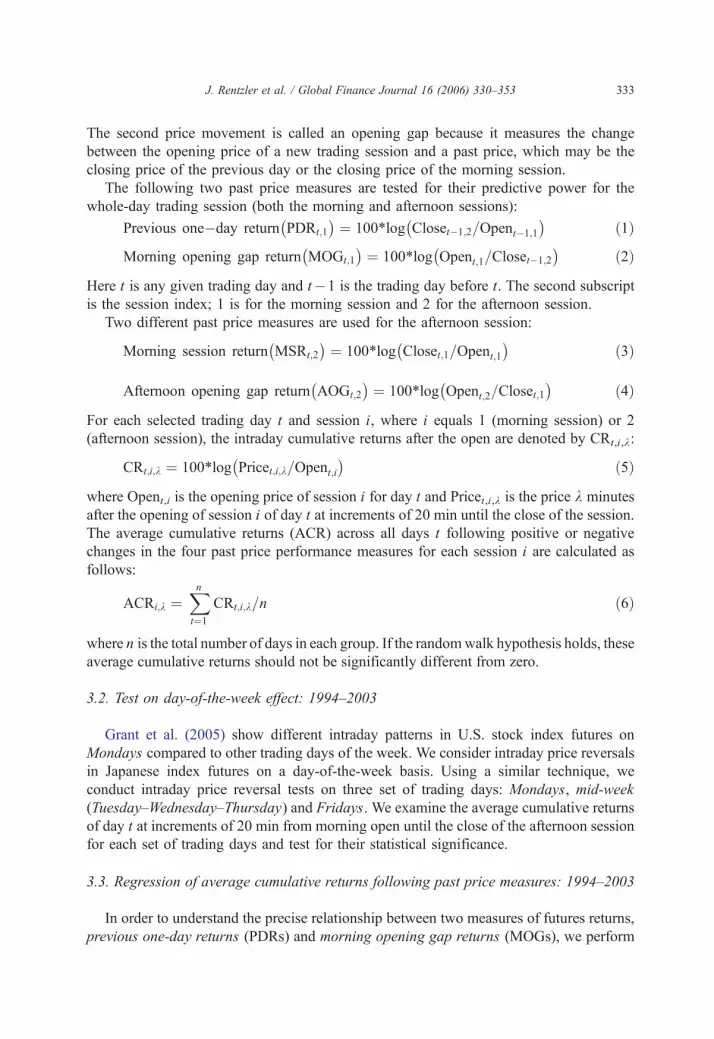
The second price movement is called an opening gap because it measures the change
between the opening price of a new trading session and a past price, which may be the
closing price of the previous day or the closing price of the morning session.
The following two past price measures are tested for their predictive power for the
whole-day trading session (both the morning and afternoon sessions):
Previous one�day return PDRt;1
� �¼ 100Tlog Closet�1;2=Opent�1;1
� �ð1Þ
Morning opening gap return MOGt;1
� �¼ 100Tlog Opent;1=Closet�1;2
� �ð2Þ
Here t is any given trading day and t�1 is the trading day before t. The second subscript
is the session index; 1 is for the morning session and 2 for the afternoon session.
Two different past price measures are used for the afternoon session:
Morning session return MSRt;2
� �¼ 100Tlog Closet;1=Opent;1
� �ð3Þ
Afternoon opening gap return AOGt;2
� �¼ 100Tlog Opent;2=Closet;1
� �ð4Þ
For each selected trading day t and session i, where i equals 1 (morning session) or 2
(afternoon session), the intraday cumulative returns after the open are denoted by CRt,i,k:
CRt;i;k ¼ 100Tlog Pricet;i;k=Opent;i� �
ð5Þ
where Opent,i is the opening price of session i for day t and Pricet,i,k is the price k minutes
after the opening of session i of day t at increments of 20 min until the close of the session.
The average cumulative returns (ACR) across all days t following positive or negative
changes in the four past price performance measures for each session i are calculated as
follows:
ACRi;k ¼Xn
t¼1CRt;i;k=n ð6Þ
where n is the total number of days in each group. If the randomwalk hypothesis holds, these
average cumulative returns should not be significantly different from zero.
3.2. Test on day-of-the-week effect: 1994–2003
Grant et al. (2005) show different intraday patterns in U.S. stock index futures on
Mondays compared to other trading days of the week. We consider intraday price reversals
in Japanese index futures on a day-of-the-week basis. Using a similar technique, we
conduct intraday price reversal tests on three set of trading days: Mondays, mid-week
(Tuesday–Wednesday–Thursday) and Fridays. We examine the average cumulative returns
of day t at increments of 20 min from morning open until the close of the afternoon session
for each set of trading days and test for their statistical significance.
3.3. Regression of average cumulative returns following past price measures: 1994–2003
In order to understand the precise relationship between two measures of futures returns,
previous one-day returns (PDRs) and morning opening gap returns (MOGs), we perform

J. Rentzler et al. / Global Finance Journal 16 (2006) 330–353334
three regressions on TOPIX and JGB futures contracts separately from 1994 to 2003 for
fourteen intraday intervals. The fourteen intraday intervals contain the points morning
open+20 min (9:00 a.m.), . . ., morning open+120 min (end of the morning session), . . .,and the interval morning open-to-afternoon close (entire trading day). Similarly, the
precise relationship between futures returns, previous morning session returns (MSRs)
and afternoon opening gap returns (AOGs) are examined in three regressions on eight
intraday intervals. The eight intraday intervals contain the points afternoon open+20 min
(12:30 p.m.), . . ., afternoon open+120 min, . . ., and the interval afternoon open-to-close
(end of the afternoon session).
The first (second) regression model (Eqs. (7) and (8)) examines the relationship
between futures returns and previous one-day return (morning opening gap return). The
third model (Eq. (9)) examines the interaction–effect relationship for futures returns with
PDRs and MOGs. The fourth (fifth) model (Eqs. (10) and (11)) examines the relationship
between futures returns and previous morning session return (afternoon opening gap
return) and the last model (Eq. (12)) examines the interaction–effect relationship for
futures returns with MSRs and AOGs. In addition, we conduct the regression analysis on
futures returns breaking each into positive or negative past price measures (Eqs. (10) and
(11). The null hypothesis for Eqs. (10) and (11 states that the slope coefficients (B1,i) are
not significantly different from zero and for Eqs. (9) and (12) states that both the slope
coefficients (B1,i and B2,i) are not significantly different from zero. The existence of a
significant intraday price pattern, following previous one-day return and/or morning
opening gap return or previous morning session return and/or afternoon opening gap
return, can be concluded if any of the slope coefficients are statistically significant. In that
case, the futures market would violate the weak-form efficiency hypothesis and
opportunities may exist for trading profits.
Ri;t ¼ B0;i þ B1;iTPDRt;1 þ ei ð7Þ
Ri;t ¼ B0;i þ B1;iTMOGt;1 þ ei ð8Þ
Ri;t ¼ B0;i þ B1;iTPDRt;1 þ B2;iTMOGt;1 þ ei ð9Þ
Ri;t ¼ B0;i þ B1;iTMSRt;2 þ ei ð10Þ
Ri;t ¼ B0;i þ B1;iTAOGt;2 þ ei ð11Þ
Ri;t ¼ B0;i þ B1;iTMSRt;1 þ B2;iTAOGt;2 þ ei ð12Þ
where,
Ri, the return of the futures contract measured from the opening to the end of the ith
intraday interval of day t.
PDRt,1 Previous one-day return. It is measured from the open of the morning session of
day t�1 to the close of the afternoon session of day t�1, where t is the day
when the intraday returns are studied.

J. Rentzler et al. / Global Finance Journal 16 (2006) 330–353 335
MOGt,1 Morning opening gap return. It is measured from the close of the afternoon
5 Data fr
session of day t�1 to the open of the morning session of day t.
MSRt,2 Previous morning session return. It is measured from the open of the morning
session of day t to the close of the morning session of day t.
AOGt,2 Afternoon opening gap return. It is measured from the close of the morning
session of day t to the open of the afternoon session of day t.
3.4. Calculation of ACRs on positive and negative extreme groups: 1994–2003
To test for the persistence of short-term inefficiencies, we adopt a strategy that looks at
extreme groupings of the ACRs. The four past performance measures are calculated and
ranked over all trading day sessions. The design of the strategy is as follows: to reduce the
effect of noise, only days with extreme past price performances are used. To achieve this,
for each of the four past performance measures, we set up two groups of trading days,
where the first group consists of days with the top 20% moves and the second group
consists of days with the bottom 20% moves. These events are hereafter called the top
20% and the bottom 20% groups, respectively.
One way to construct the top and bottom 20% groups is to look at the distribution of
each past price movement over the entire sample period and use the distribution’s 80th
percentile and 20th percentile as cutoff points. While this method guarantees an allocation
of exactly 20% of all trading days to each of the two groups, it has a drawback. It commits
a fallacy of prophecy since it assumes that we know in advance the distribution of the price
movements over the 11-year period.
We use an adaptive filter rule that considers only the distribution of the previous year’s
price movements and uses the 80th percentile and the 20th percentile in determining the
event days for the current year. This results in the loss of one year of data, leaving us with ten
years of event day data.5 As long as the distribution does not shift dramatically year over
year, this method still generates approximately 20% of trading days for each of the two
extreme groups.
In addition to the percentage cumulative returns, we adopt tick-size cumulative moves for
three reasons. First, it is easier to convert tick-size gains (or losses) into yen terms for any
given percentage gain (or loss). Second, since futures contracts are secured with initial
margin and no investment is required, percentage movements in prices are not a trader’s
actual rate of return. Third, transaction costs are easy to incorporate when the gains (or
losses) are in tick-size.
4. Empirical results
4.1. Results on average cumulative returns following positive and negative past price
measures: 1994–2003
Table 1 presents the average cumulative return (in percent) and the significance tests (2-
tailed t-test and Wilcoxon signed rank test) performed on TOPIX futures and 10-year JGB
om 1993 is used to calculate the 80th percentile and 20th percentile cutoff points for 1994 only.

Table 1
Average cumulative return (%) on TOPIX futures and 10-year JGB futures following all positive or all negative past price measures from 1994 to 2003
Panel A: Average cumulative returns in morning and afternoon sessions following previous one-day returns and morning opening gap
Average cumulative returns on TOPIX futures Average cumulative returns on 10-year JGB futures
Previous one-day returna Morning opening gapb Previous one day returna Morning opening gapb
Positive Negative Positive Negative Positive Negative Positive Negative
Number of
days
1095 1288 1244 1055 1289 1089 1222 1094
Intraday
periods
ACR (%) Wilcoxon ACR (%) Wilcoxon ACR (%) Wilcoxon ACR (%) Wilcoxon ACR (%) Wilcoxon ACR (%) Wilcoxon ACR (%) Wilcoxon ACR (%) Wilcoxon
900–920 �0.013 1.45 �0.038*** 4.16*** �0.073*** 7.66*** 0.027*** 2.32** 0.008*** 3.35*** �0.003 0.70 �0.005** 2.42** 0.012*** 5.06***
900–940 �0.017* 1.83* �0.043*** 3.67*** �0.107*** 8.78*** 0.050*** 3.16*** 0.008*** 2.28** �0.002 0.63 �0.008*** 2.35** 0.016*** 5.31***
900–1000 �0.019* 1.75* �0.037*** 2.49** �0.103*** 7.22*** 0.059*** 3.15*** 0.007** 1.98** 0.001 1.84* �0.005* 1.16 0.016*** 5.29***
900–1020 �0.020 1.48 �0.049*** 2.81*** �0.106*** 6.56*** 0.050*** 2.49** 0.004 0.64 �0.001 0.58 �0.010*** 2.75*** 0.015*** 4.22***
900–1040 �0.016 1.16 �0.068*** 3.59*** �0.102*** 6.00*** 0.031* 1.48 0.004 0.98 �0.001 0.51 �0.009*** 1.93* 0.014*** 3.87***
900–1100 �0.044** 2.28** �0.084*** 4.14*** �0.117*** 5.97*** �0.001 0.28 0.001 0.50 0.001 1.18 �0.008** 1.01 0.014*** 3.40***
900–1250 �0.084*** 4.13*** �0.124*** 5.56*** �0.169*** 7.82*** �0.024 1.56 0.004 1.01 0.012** 3.33*** �0.004 0.22 0.023*** 5.06***
900–1310 �0.078*** 3.65*** �0.123*** 5.31*** �0.166*** 7.22*** �0.021 1.44 0.004 1.27 0.015*** 3.93*** �0.005 0.12 0.029*** 5.95***
900–1330 �0.071*** 3.36*** �0.107*** 4.67*** �0.156*** 6.66*** �0.004 0.98 0.004 1.34 0.017*** 4.15*** �0.005 0.02 0.030*** 5.89***
900–1350 �0.067*** 3.06*** �0.111*** 4.73*** �0.148*** 6.11*** �0.012 1.29 0.004 1.19 0.019*** 4.50*** �0.003 0.26 0.031*** 5.87***
900–1410 �0.073*** 3.20*** �0.117*** 4.83*** �0.153*** 6.24*** �0.020 1.38 0.005 1.28 0.018*** 4.28*** �0.002 0.56 0.030*** 5.37***
900–1430 �0.077*** 3.21*** �0.106*** 3.94*** �0.137*** 5.24*** �0.029 1.47 0.005 1.67* 0.021*** 4.61*** �0.002 1.11 0.032*** 5.54***
900–1450 �0.104*** 3.94*** �0.095*** 3.51*** �0.146*** 5.37*** �0.032 1.45 0.003 1.26 0.028*** 5.25*** 0.003 1.46 0.030*** 5.05***
900–Close �0.131*** 4.69*** �0.052* 1.72* �0.127*** 4.24*** �0.034 1.55 �0.001 0.63 0.027*** 4.99*** 0.010* 2.70*** 0.016** 2.88***
J.Rentzler
etal./GlobalFinance
Journal16(2006)330–353
336

B: Average cumulative returns in afternoon sessions following morning session returns and afternoon opening gap
Average cumulative returns on TOPIX futures Average cumulative returns on 10-year JGB futures
Morning session returnc Afternoon opening gapd Morning session returnc Afternoon opening gapd
Positive Negative Positive Negative Positive Negative Positive Negative
Number of
days
1074 1249 946 1452 1215 1124 1275 1080
Intraday
periods
ACR (%) Wilcoxon ACR (%) Wilcoxon ACR (%) Wilcoxon ACR (%) Wilcoxon ACR (%) Wilcoxon ACR (%) Wilcoxon ACR (%) Wilcoxon ACR (%) Wilcoxon
1230–1250 0.015** 1.05 �0.031*** 3.84*** 0.030*** 3.24*** �0.033*** 5.07*** 0.001 0.22 0.008*** 4.92*** 0.006*** 3.20*** 0.002 1.77*
1230–1310 0.019** 1.70* �0.028*** 2.64*** 0.049*** 4.52*** �0.040*** 4.45*** 0.001 0.41 0.012*** 5.97*** 0.007*** 2.74*** 0.005** 3.63***
1230–1330 0.031** 2.10** �0.016* 1.04 0.061*** 5.23*** �0.029*** 3.18*** 0.002 0.29 0.014*** 6.48*** 0.008*** 3.29*** 0.007** 3.81***
1230–1350 0.020* 1.16 �0.009 0.30 0.070*** 4.93*** �0.036*** 3.13*** 0.002 0.47 0.015*** 5.82*** 0.009*** 2.74*** 0.008** 3.63***
1230–1410 0.012 0.21 �0.007 0.01 0.073*** 4.50*** �0.045*** 3.45*** 0.001 0.03 0.016*** 5.60*** 0.008*** 2.57** 0.009** 3.09***
1230–1430 0.019 0.64 �0.005 0.18 0.078*** 4.14*** �0.042*** 2.97*** 0.004 1.39 0.016*** 5.14*** 0.012*** 3.79*** 0.007** 2.84***
1230–1450 0.012 0.31 �0.008 0.73 0.084*** 3.47*** �0.055*** 3.28*** 0.005 1.49 0.019*** 4.67*** 0.014*** 3.57*** 0.008* 2.30**
1230–close 0.036* 0.87 �0.012 1.08 0.095*** 2.78*** �0.048** 2.52** 0.003 1.25 0.014** 3.43*** 0.010** 2.99*** 0.006 1.59
Wilcoxon: two-tailed signed rank test (H0: median is not zero).a Previous one-day return (PDRt ,1)=100* log(Closet�1,2/Opent�1,1).b Morning opening gap (MOGt ,1)=100* log(Opent ,1/Closet�1,2).c Morning session return (MSRt ,2)=100* log(Closet ,1/Opent ,1).d Afternoon opening gap (AOGt ,2)=100* log(Opent ,2/Closet ,1), where 1=morning, 2=afternoon.
* Significant at 10% significance level.
** Significant at 5% significance level.
*** Significant at 1% significance level.
J.Rentzler
etal./GlobalFinance
Journal16(2006)330–353
337

J. Rentzler et al. / Global Finance Journal 16 (2006) 330–353338
futures following positive/negative past price measures. Panel A indicates the average
cumulative returns (ACRs) following previous one-day return and morning opening gap
return over the entire trading day, while Panel B presents the ACRs for the afternoon
sessions following morning session return and afternoon opening gap return. In each
panel, Columns 1–4 present the returns on TOPIX futures and Columns 5–8 the returns on
10-year JGB futures.
4.1.1. A1 TOPIX futures
Regarding the previous one-day return, Table 1 (Columns 1 and 3) shows that the
average cumulative returns on TOPIX futures are significantly negative for the positive
group (Column 1) indicating reversals and negative for the negative group (Column 3)
indicating persistence. Morning opening gap returns (Columns 5 and 7) are significantly
negative for the positive group and significantly positive for the negative group, indicating
significant reversals in both cases. This provides strong support for intraday market
inefficiency and is consistent with the findings for other future indices (e.g. Fung et al.
(2000) and Grant et al. (2005)).
We then use MSRs and AOGs for TOPIX futures, which combine the morning
session’s information with the afternoon opening prices to create a similar analysis using
only the afternoon session’s data (Table 1, Panel B). Both measures, MSR and AOG,
exhibit significant positive (negative) cumulative returns following positive (negative) past
price measure, indicating strong and significant price persistence patterns. While
significant ACRs following morning session return are observed in the first hour of the
afternoon session, the afternoon opening gap extends this significant positive relationship
over the entire afternoon session. This implies that the trading of TOPIX futures in the
afternoon is strongly influenced by trading in its morning session.
4.1.2. A2 JGB futures
Results on the 10-year JGB futures are presented in Table 1, Columns 9–16 (Panels A
and B). In Panel A, we observe significant persistence for positive previous one-day
return in the opening minutes, significant reversal in the afternoon trading session for
negative PDRs, and strong and significant reversals for positive and negative MOGs.
Panel B presents the price patterns for the afternoon session. Here we find that morning
session returns (Panel B, Columns 9 and 11) indicate significant reversals for the
negative group as observed by significantly positive ACRs but no pattern is observed for
the positive group. Examining the afternoon opening gap return (Panel B, Columns 13
and 15), the 10-year JGB futures exhibit significant positive cumulative returns for both
the positive and negative group. Therefore, for the positive group, the afternoon session
shows persistence while the morning session displays reversals. The negative group
continues to exhibit the same reversal pattern in both the morning and afternoon
sessions.
Summarizing, we find significant reversals or persistence patterns for TOPIX futures
for all eight measures (both positive and negative groups), while for 10-year JGB futures,
we find significant reversals or persistence patterns in seven of eight cases. The ACRs are
stronger for TOPIX futures. We also find that investors generally tend to overreact to
morning session openings (Panel A shows significant reversals in six of eight cases) and

Table 2
Regression analyses between intraday cumulative returns and past price measures (previous day return, morning
opening gap, previous morning session return and afternoon opening gap) on TOPIX index futures (1994–2003)
Panel A: Entire trading days (following PDRa and MOGb)
Intraday
periods
Following PDR Following MOG Following PDR and MOG
a b a d a b d
900–920 �0.0284*** 0.0020 �0.0238*** �0.0649*** �0.0237*** 0.0009 �0.0649***900–940 �0.0308*** 0.0021 �0.0234*** �0.1029*** �0.0234*** 0.0004 �0.1029***900–1000 �0.0274*** �0.0075 �0.0185* �0.1112*** �0.0193** �0.0093 �0.1115***900–1020 �0.0313*** �0.0041 �0.0237** �0.0981*** �0.0242** �0.0058 �0.0983**900–1040 �0.0371*** 0.0032 �0.0321** �0.0707*** �0.0319** 0.0020 �0.0707***900–1100 �0.0607*** �0.0002 �0.0561*** �0.0625*** �0.0562*** �0.0012 �0.0625***900–1250 �0.1002*** 0.0081 �0.0945*** �0.0867*** �0.0940*** 0.0066 �0.0865***900–1310 �0.0982*** 0.0061 �0.0925*** �0.0849*** �0.0921*** 0.0047 �0.0847***900–1330 �0.0869*** �0.0010 �0.0803*** �0.0879*** �0.0805*** �0.0025 �0.0880***900–1350 �0.0847*** 0.0011 �0.0786*** �0.0837*** �0.0786*** �0.0003 �0.0837***900–1410 �0.0912*** 0.0049 �0.0852*** �0.0875*** �0.0849*** 0.0034 �0.0874***900–1430 �0.0887*** �0.0024 �0.0835*** �0.0678*** �0.0838*** �0.0036 �0.0679***900–1450 �0.0978*** �0.0314* �0.0901*** �0.0666*** �0.0929*** �0.0325* �0.0676***900–1510 �0.0878*** �0.0736*** �0.0781 �0.0445* �0.0844*** �0.0744*** �0.0468*
Panel B: Afternoon sessions (following MSRc and AOGd)
Intraday
periods
Following MSR Following AOG Following MSR and AOG
a b a d a b d
1230–1250 �0.0084 0.0405*** �0.0059 0.1424*** �0.0041 0.0385*** 0.1353***
1230–1310 �0.0049 0.0384*** �0.0010 0.1816*** 0.0007 0.0358*** 0.1750***
1230–1330 0.0046 0.0314*** 0.0080 0.1546*** 0.0093 0.0292*** 0.1492***
1230–1350 0.0049 0.0177 0.0085 0.1408*** 0.0093 0.0157 0.1379***
1230–1410 �0.0005 0.0153 0.0049 0.1898*** 0.0055 0.0125 0.1875***
1230–1430 0.0029 0.0344** 0.0082 0.2184*** 0.0097 0.0313** 0.2126***
1230–1450 �0.0050 0.0204 0.0024 0.2590*** 0.0032 0.0167 0.2560***
1230–1510 0.0107 0.0510** 0.0168 0.2690*** 0.0191 0.0472** 0.2603***
Regression analyses are conducted on each (i) of the 14 (or 8 afternoon session) intraday cumulative returns
(CRi ,t) against each of the following equations:
CRi;t ¼ ai þ bi PDRt;1
� �þ ei:
CRi;t ¼ ai þ di MOGt;1
� �þ ei:
CRi;t ¼ ai þ bi PDRt;1
� �þ di MOGt;1
� �þ ei:
CRi;t ¼ ai þ bi MSRt;2
� �þ ei:
CRi;t ¼ ai þ di AOGt;2
� �þ ei:
CRi;t ¼ ai þ bi MSRt;2
� �þ di AOGt;2
� �þ ei:
a Previous one-day return (PDRt ,1)=100* log(Closet�1,2/Opent�1,1).b Morning opening gap (MOGt ,1)=100* log(Opent ,1/Closet�1,2).c Morning session return (MSRt ,2)=100* log(Closet ,1/Opent ,1).d Afternoon opening gap (AOGt ,2)=100* log(Opent ,2/Closet ,1), where 1=morning, 2=afternoon.
* Significant at 10% significance level.
** Significant at 5% significance level.
*** Significant at 1% significance level.
J. Rentzler et al. / Global Finance Journal 16 (2006) 330–353 339
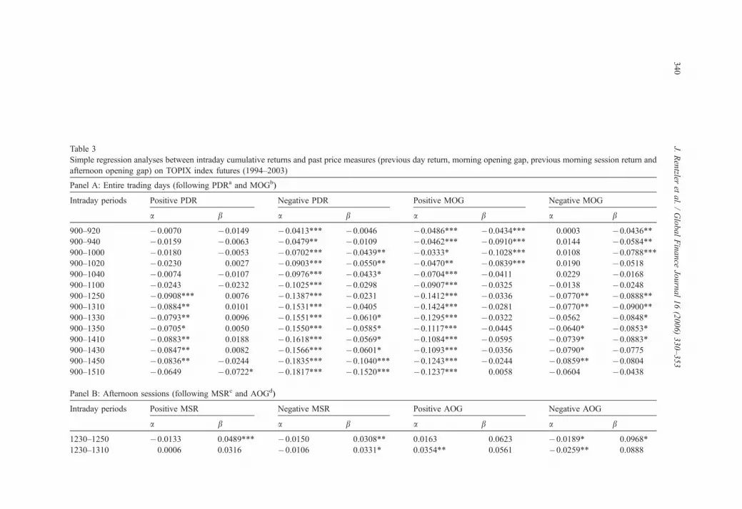
Table 3
Simple regression analyses between intraday cumulative returns and past price measures (previous day return, morning opening gap, previous morning session return and
afternoon opening gap) on TOPIX index futures (1994–2003)
Panel A: Entire trading days (following PDRa and MOGb)
Intraday periods Positive PDR Negative PDR Positive MOG Negative MOG
a b a b a b a b
900–920 �0.0070 �0.0149 �0.0413*** �0.0046 �0.0486*** �0.0434*** 0.0003 �0.0436**900–940 �0.0159 �0.0063 �0.0479** �0.0109 �0.0462*** �0.0910*** 0.0144 �0.0584**900–1000 �0.0180 �0.0053 �0.0702*** �0.0439** �0.0333* �0.1028*** 0.0108 �0.0788***900–1020 �0.0230 0.0027 �0.0903*** �0.0550** �0.0470** �0.0839*** 0.0190 �0.0518900–1040 �0.0074 �0.0107 �0.0976*** �0.0433* �0.0704*** �0.0411 0.0229 �0.0168900–1100 �0.0243 �0.0232 �0.1025*** �0.0298 �0.0907*** �0.0325 �0.0138 �0.0248900–1250 �0.0908*** 0.0076 �0.1387*** �0.0231 �0.1412*** �0.0336 �0.0770** �0.0888**900–1310 �0.0884** 0.0101 �0.1531*** �0.0405 �0.1424*** �0.0281 �0.0770** �0.0900**900–1330 �0.0793** 0.0096 �0.1551*** �0.0610* �0.1295*** �0.0322 �0.0562 �0.0848*900–1350 �0.0705* 0.0050 �0.1550*** �0.0585* �0.1117*** �0.0445 �0.0640* �0.0853*900–1410 �0.0883** 0.0188 �0.1618*** �0.0569* �0.1084*** �0.0595 �0.0739* �0.0883*900–1430 �0.0847** 0.0082 �0.1566*** �0.0601* �0.1093*** �0.0356 �0.0790* �0.0775900–1450 �0.0836** �0.0244 �0.1835*** �0.1040*** �0.1243*** �0.0244 �0.0859** �0.0804900–1510 �0.0649 �0.0722* �0.1817*** �0.1520*** �0.1237*** 0.0058 �0.0604 �0.0438
Panel B: Afternoon sessions (following MSRc and AOGd)
Intraday periods Positive MSR Negative MSR Positive AOG Negative AOG
a b a b a b a b
1230–1250 �0.0133 0.0489*** �0.0150 0.0308** 0.0163 0.0623 �0.0189* 0.0968*
1230–1310 0.0006 0.0316 �0.0106 0.0331* 0.0354** 0.0561 �0.0259** 0.0888
J.Rentzler
etal./GlobalFinance
Journal16(2006)330–353
340

1230–1330 0.0058 0.0405 �0.0248 �0.0086 0.0584*** �0.0257 �0.0228 0.0446
1230–1350 0.0121 0.0122 �0.0127 �0.0028 0.0746*** �0.0955 �0.0348** �0.01461230–1410 0.0088 0.0027 �0.0022 0.0157 0.0646*** �0.0223 �0.0364** 0.0400
1230–1430 0.0007 0.0313 0.0231 0.0605* 0.0755*** �0.0555 �0.0229 0.1334
1230–1450 0.0013 0.0082 0.0121 0.0432 0.0844*** �0.0952 �0.0230 0.2177*
1230–1510 0.0166 0.0374 0.0324 0.0802* 0.1051*** �0.1224 �0.0109 0.2299
Simple regression analyses are conducted on each (i) of the 14 (or 8 in afternoon session) intraday cumulative returns (CRi ,t) against one of the four past price measures.
Each past price measure is separated into positive and negative groups. The simple regressions are as follows:
CRi;t ¼ ai þ bi PDRt;1
� �þ ei:
CRi;t ¼ ai þ di MOGt;1
� �þ ei:
CRi;t ¼ ai þ bi MSRt;2
� �þ ei:
CRi;t ¼ ai þ di AOGt;2
� �þ ei:
a Previous one-day return (PDRt ,1)=100* log(Closet�1,2/Opent�1,1).b Morning opening gap (MOGt ,1)=100*log(Opent ,1/Closet�1,2).c Morning session return (MSRt ,2)=100* log(Closet ,1/Opent ,1).d Afternoon opening gap (AOGt ,2)=100* log(Opent ,2/Closet ,1), where 1=morning, 2=afternoon.
* Significant at 10% significance level.
** Significant at 5% significance level.
*** Significant at 1% significance level.
J.Rentzler
etal./GlobalFinance
Journal16(2006)330–353
341
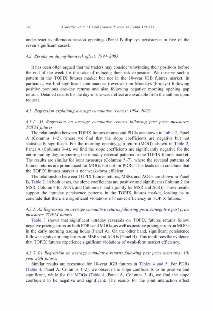
J. Rentzler et al. / Global Finance Journal 16 (2006) 330–353342
under-react to afternoon session openings (Panel B displays persistence in five of the
seven significant cases).
4.2. Results on day-of-the-week effect: 1994–2003
It has been often argued that the traders may consider unwinding their positions before
the end of the week for the sake of reducing their risk exposures. We observe such a
pattern in the TOPIX futures market but not in the 10-year JGB futures market. In
particular, we find significant continuances (reversals) on Mondays (Fridays) following
positive previous one-day returns and also following negative morning opening gap
returns. Detailed results for the day-of-the-week effect are available from the authors upon
request.
4.3. Regression explaining average cumulative returns: 1994–2003
4.3.1. A1 Regression on average cumulative returns following past price measures:
TOPIX futures
The relationship between TOPIX futures returns and PDRs are shown in Table 2, Panel
A (Columns 1–2), where we find that the slope coefficients are negative but not
statistically significant. For the morning opening gap return (MOG), shown in Table 2,
Panel A (Columns 3–4), we find the slope coefficients are significantly negative for the
entire trading day, supporting the intraday reversal patterns in the TOPIX futures market.
The results are similar for joint measures (Columns 5–7), where the reversal patterns of
futures returns are pronounced for MOGs but not for PDRs. This leads us to conclude that
the TOPIX futures market is not weak-form efficient.
The relationship between TOPIX futures returns, MSRs and AOGs are shown in Panel
B, Table 2. In both cases, the slope coefficients are positive and significant (Column 2 for
MSR, Column 4 for AOG, and Columns 6 and 7 jointly for MSR and AOG). These results
support the intraday persistence patterns in the TOPIX futures market, leading us to
conclude that there are significant violations of market efficiency in TOPIX futures.
4.3.2. A2 Regression on average cumulative returns following positive/negative past price
measures: TOPIX futures
Table 3 shows that significant intraday reversals on TOPIX futures returns follow
negative pricing errors on both PDRs andMOGs, as well as positive pricing errors onMOGs
in the early morning trading hours (Panel A). On the other hand, significant persistence
follows negative pricing errors on MSRs and AOGs (Panel B). This reinforces the evidence
that TOPIX futures experience significant violations of weak-form market efficiency.
4.3.3. B1 Regression on average cumulative returns following past price measures: 10-
year JGB futures
Similar results are presented for 10-year JGB futures in Tables 4 and 5. For PDRs
(Table 4, Panel A, Columns 1–2), we observe the slope coefficients to be positive and
significant, while for the MOGs (Table 4, Panel A, Columns 3–4), we find the slope
coefficient to be negative and significant. The results for the joint interaction effect

Table 4
Regression analyses between intraday cumulative returns and past price measures (previous day return, morning
opening gap, previous morning session return, and afternoon opening gap) on 10-year JGB futures (1994–2003)
Panel A: Entire trading days (following PDRa and MOGb)
Intraday
periods
Following PDR Following MOG Following PDR and MOG
a b a d a b d
900–920 0.0038** 0.0338*** 0.0046*** �0.0441*** 0.0042** 0.0345*** �0.0451***900–940 0.0041** 0.0358*** 0.0052** �0.0717*** 0.0048** 0.0369*** �0.0728***900–1000 0.0051** 0.0333*** 0.0060*** �0.0649*** 0.0056** 0.0343*** �0.0659***900–1020 0.0028 0.0256*** 0.0037 �0.0704*** 0.0034 0.0267*** �0.0712***900–1040 0.0037 0.0186* 0.0044 �0.0544*** 0.0042 0.0194* �0.0549***900–1100 0.0034 0.0014 0.0039 �0.0509*** 0.0038 0.0022 �0.0510***900–1250 0.0080** �0.0097 0.0084** �0.0502*** 0.0085** �0.0089 �0.0499***900–1310 0.0100*** �0.0172 0.0105*** �0.0788*** 0.0107*** �0.0160 �0.0783***900–1330 0.0113*** �0.0194 0.0118*** �0.0779*** 0.0120*** �0.0182 �0.0774***900–1350 0.0128*** �0.0217 0.0132*** �0.0722*** 0.0134*** �0.0205 �0.0716***900–1410 0.0127*** �0.0203 0.0131*** �0.0728*** 0.0134*** �0.0192 �0.0722***900–1430 0.0144*** �0.0291* 0.0147*** �0.0710*** 0.0150*** �0.0280* �0.0702***900–1450 0.0154*** �0.0448** 0.0153*** �0.0448* 0.0158*** �0.0441** �0.0435*900–1500 0.0124** �0.0616*** 0.0116** 0.0059 0.0123** �0.0618*** 0.0077
Panel B: Afternoon sessions (following MSRc and AOGd)
Intraday
periods
Following MSR Following AOG Following MSR and AOG
a b a d a b d
1230–1250 0.0037*** �0.0471*** 0.0035*** 0.0138 0.0036*** �0.0473*** 0.0148
1230–1310 0.0055*** �0.0624*** 0.0053*** 0.0161 0.0055*** �0.0625*** 0.0175
1230–1330 0.0070*** �0.0677*** 0.0067*** 0.0179 0.0069*** �0.0679*** 0.0194
1230–1350 0.0085*** �0.0857*** 0.0082*** 0.0241 0.0084*** �0.0860*** 0.0260
1230–1410 0.0086*** �0.0766*** 0.0083*** 0.0338* 0.0085*** �0.0769*** 0.0355*
1230–1430 0.0102*** �0.0591*** 0.0099*** 0.0379 0.0100*** �0.0595*** 0.0392*
1230–1450 0.0109*** �0.0645*** 0.0107*** 0.0060 0.0108*** �0.0646*** 0.0074
1230–1500 0.0077** �0.0366 0.0075** 0.0128 0.0076** �0.0367 0.0136
Regression analyses are conducted on each (i) of the 14 (or 8 in afternoon session) intraday cumulative returns
(CRi ,t) against each of the following equations,
CRi;t ¼ ai þ bi PDRt;1
� �þ ei:
CRi;t ¼ ai þ di MOGt;1
� �þ ei:
CRi;t ¼ ai þ bi PDRt;1
� �þ di MOGt;1
� �þ ei:
CRi;t ¼ ai þ bi MSRt;2
� �þ ei:
CRi;t ¼ ai þ di AOGt;2
� �þ ei:
CRi;t ¼ ai þ bi MSRt;2
� �þ di AOGt;2
� �þ ei:
a Previous one-day return (PDRt ,1)=100* log(Closet�1,2/Opent�1,1).b Morning opening gap (MOGt ,1)=100* log(Opent ,1/Closet�1,2).c Morning session return (MSRt ,2)=100* log(Closet ,1/Opent ,1).d Afternoon opening gap (AOGt ,2)=100* log(Opent ,2/Closet ,1), where 1=morning, 2=afternoon.
* Significant at 10% significance level.
** Significant at 5% significance level.
*** Significant at 1% significance level.
J. Rentzler et al. / Global Finance Journal 16 (2006) 330–353 343

Table 5
Simple regression analyses between intraday cumulative returns and past price measures (previous day return, morning opening gap, previous morning session return and
afternoon opening gap) on 10-year JGB futures (1994–2003)
Panel A: Entire trading days (following PDRa and MOGb)
Intraday
periods
Positive PDR Negative PDR Positive MOG Negative MOG
a b a b a b a b
900–920 0.0064* 0.0146 0.0082** 0.0558*** �0.0002 �0.0254 0.0080** �0.0340*900–940 0.0075* 0.0065 0.0141*** 0.0792*** �0.0027 �0.0370* 0.0084* �0.0690***900–1000 0.0055 0.0154 0.0165*** 0.0781*** �0.0028 �0.0199 0.0083* �0.0737***900–1020 0.0048 0.0048 0.0123** 0.0636*** �0.0044 �0.0379 0.0104** �0.0513*900–1040 0.0079 �0.0068 0.0076 0.0405* �0.0051 �0.0228 0.0159*** �0.0104900–1100 0.0075 �0.0254 0.0062 0.0223 �0.0069 �0.0035 0.0114* �0.0354900–1250 0.0083 �0.0197 0.0121 0.0093 �0.0058 0.0135 0.0187** �0.0299900–1310 0.0126* �0.0403 0.0160** 0.0124 �0.0031 �0.0130 0.0182** �0.0733*900–1330 0.0156** �0.0546* 0.0205** 0.0250 �0.0033 �0.0074 0.0210*** �0.0662900–1350 0.0190** �0.0689** 0.0243*** 0.0346 �0.0022 �0.0006 0.0235*** �0.0570900–1410 0.0194** �0.0684** 0.0243*** 0.0353 0.0001 �0.0149 0.0240*** �0.0481900–1430 0.0189** �0.0658* 0.0246*** 0.0187 0.0010 �0.0123 0.0271*** �0.0391900–1450 0.0188** �0.0784** 0.0290*** 0.0119 0.0015 0.0111 0.0293*** �0.0031900–1500 0.0197* �0.1077*** 0.0228** �0.0124 0.0052 0.0360 0.0180 0.0197
Panel B: Afternoon sessions (following MSRc and AOGd)
Intraday
periods
Positive MSR Negative MSR Positive AOG Negative AOG
a b a b a b a b
1230–1250 0.0068*** �0.0500*** �0.0039 �0.0876*** 0.0045** 0.0169 0.0013 �0.00331230–1310 0.0079*** �0.0596*** �0.0007 �0.0990*** 0.0054** 0.0157 0.0055** 0.0171
J.Rentzler
etal./GlobalFinance
Journal16(2006)330–353
344

1230–1330 0.0087** �0.0584*** �0.0002 �0.1114*** 0.0070*** 0.0114 0.0081*** 0.0312
1230–1350 0.0104*** �0.0686*** �0.0036 �0.1568*** 0.0073** 0.0226 0.0107*** 0.0390
1230–1410 0.0098** �0.0717** 0.0039 �0.1047*** 0.0067* 0.0172 0.0136*** 0.0845**
1230–1430 0.0104* �0.0489 0.0059 �0.0863*** 0.0104** 0.0202 0.0123*** 0.0708*
1230–1450 0.0135** �0.0748* 0.0104 �0.0681* 0.0145*** �0.0593 0.0138*** 0.0980**
1230–1500 0.0109 �0.0663 0.0109 �0.0105 0.0097* �0.0527 0.0126** 0.1191**
Simple regression analyses are conducted on each (i) of the 14 (or 8 in afternoon session) intraday cumulative returns (CRi ,t) against one of the four past price measures.
Each past price measure is separated into positive and negative groups. The simple regressions are as follows:
CRi;t ¼ ai þ bi PDRt;1
� �þ ei:
CRi;t ¼ ai þ di MOGt;1
� �þ ei:
CRi;t ¼ ai þ bi MSRt;2
� �þ ei:
CRi;t ¼ ai þ di AOGt;2
� �þ ei:
a Previous one-day return (PDRt ,1)=100* log(Closet�1,2/Opent�1,1).b Morning opening gap (MOGt ,1)=100* log(Opent ,1/Closet�1,2).c Morning session return (MSRt ,2)=100*log(Closet ,1/Opent ,1).d Afternoon opening gap (AOGt ,2)=100* log(Opent ,2/Closet ,1), where 1=morning, 2=afternoon.
* Significant at 10% significance level.
** Significant at 5% significance level.
*** Significant at 1% significance level.
J.Rentzler
etal./GlobalFinance
Journal16(2006)330–353
345
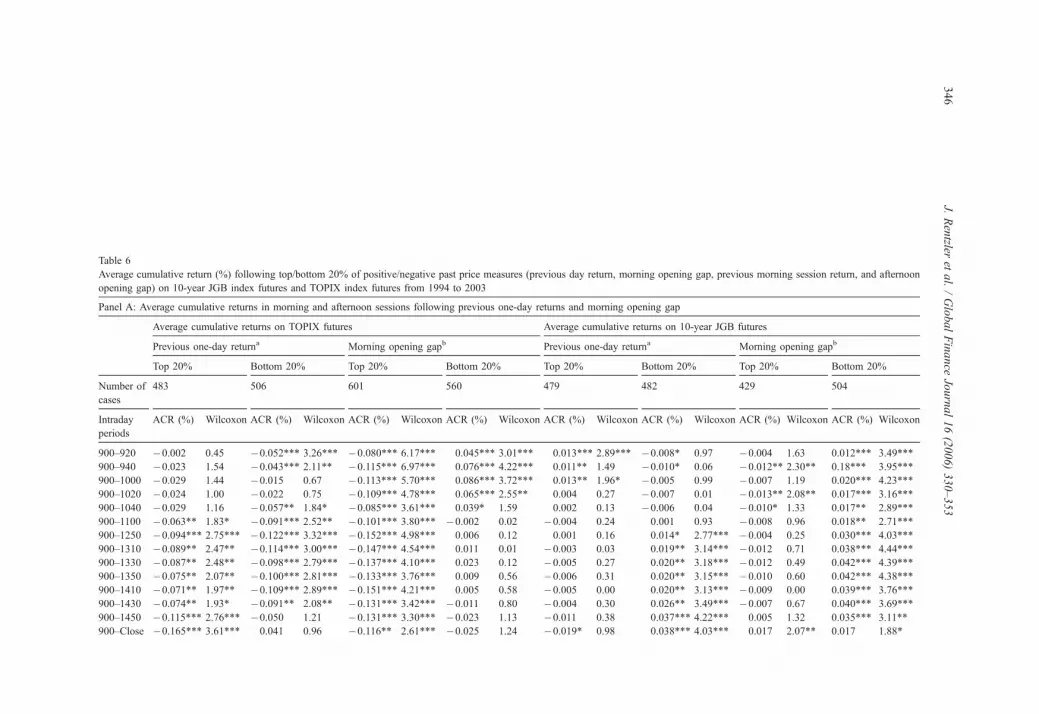
Table 6
Average cumulative return (%) following top/bottom 20% of positive/negative past price measures (previous day return, morning opening gap, previous morning session return, and afternoon
opening gap) on 10-year JGB index futures and TOPIX index futures from 1994 to 2003
Panel A: Average cumulative returns in morning and afternoon sessions following previous one-day returns and morning opening gap
Average cumulative returns on TOPIX futures Average cumulative returns on 10-year JGB futures
Previous one-day returna Morning opening gapb Previous one-day returna Morning opening gapb
Top 20% Bottom 20% Top 20% Bottom 20% Top 20% Bottom 20% Top 20% Bottom 20%
Number of
cases
483 506 601 560 479 482 429 504
Intraday
periods
ACR (%) Wilcoxon ACR (%) Wilcoxon ACR (%) Wilcoxon ACR (%) Wilcoxon ACR (%) Wilcoxon ACR (%) Wilcoxon ACR (%) Wilcoxon ACR (%) Wilcoxon
900–920 �0.002 0.45 �0.052*** 3.26*** �0.080*** 6.17*** 0.045*** 3.01*** 0.013*** 2.89*** �0.008* 0.97 �0.004 1.63 0.012*** 3.49***
900–940 �0.023 1.54 �0.043*** 2.11** �0.115*** 6.97*** 0.076*** 4.22*** 0.011** 1.49 �0.010* 0.06 �0.012** 2.30** 0.18*** 3.95***
900–1000 �0.029 1.44 �0.015 0.67 �0.113*** 5.70*** 0.086*** 3.72*** 0.013** 1.96* �0.005 0.99 �0.007 1.19 0.020*** 4.23***
900–1020 �0.024 1.00 �0.022 0.75 �0.109*** 4.78*** 0.065*** 2.55** 0.004 0.27 �0.007 0.01 �0.013** 2.08** 0.017*** 3.16***
900–1040 �0.029 1.16 �0.057** 1.84* �0.085*** 3.61*** 0.039* 1.59 0.002 0.13 �0.006 0.04 �0.010* 1.33 0.017** 2.89***
900–1100 �0.063** 1.83* �0.091*** 2.52** �0.101*** 3.80*** �0.002 0.02 �0.004 0.24 0.001 0.93 �0.008 0.96 0.018** 2.71***
900–1250 �0.094*** 2.75*** �0.122*** 3.32*** �0.152*** 4.98*** 0.006 0.12 0.001 0.16 0.014* 2.77*** �0.004 0.25 0.030*** 4.03***
900–1310 �0.089** 2.47** �0.114*** 3.00*** �0.147*** 4.54*** 0.011 0.01 �0.003 0.03 0.019** 3.14*** �0.012 0.71 0.038*** 4.44***
900–1330 �0.087** 2.48** �0.098*** 2.79*** �0.137*** 4.10*** 0.023 0.12 �0.005 0.27 0.020** 3.18*** �0.012 0.49 0.042*** 4.39***
900–1350 �0.075** 2.07** �0.100*** 2.81*** �0.133*** 3.76*** 0.009 0.56 �0.006 0.31 0.020** 3.15*** �0.010 0.60 0.042*** 4.38***
900–1410 �0.071** 1.97** �0.109*** 2.89*** �0.151*** 4.21*** 0.005 0.58 �0.005 0.00 0.020** 3.13*** �0.009 0.00 0.039*** 3.76***
900–1430 �0.074** 1.93* �0.091** 2.08** �0.131*** 3.42*** �0.011 0.80 �0.004 0.30 0.026** 3.49*** �0.007 0.67 0.040*** 3.69***
900–1450 �0.115*** 2.76*** �0.050 1.21 �0.131*** 3.30*** �0.023 1.13 �0.011 0.38 0.037*** 4.22*** 0.005 1.32 0.035*** 3.11**
900–Close �0.165*** 3.61*** 0.041 0.96 �0.116** 2.61*** �0.025 1.24 �0.019* 0.98 0.038*** 4.03*** 0.017 2.07** 0.017 1.88*
J.Rentzler
etal./GlobalFinance
Journal16(2006)330–353
346

Panel B: Average cumulative returns in afternoon sessions following morning session returns and afternoon opening gap
Average cumulative returns on TOPIX futures Average cumulative returns on 10-year JGB futures
Morning session returnc Afternoon opening gapd Morning session returnc Afternoon opening gapd
Top 20% Bottom 20% Top 20% Bottom 20% Top 20% Bottom 20% Top 20% Bottom 20%
Number of
cases
492 528 552 516 473 469 472 425
Intraday
periods
ACR (%) Wilcoxon ACR (%) Wilcoxon ACR (%) Wilcoxon ACR (%) Wilcoxon ACR (%) Wilcoxon ACR (%) Wilcoxon ACR (%) Wilcoxon ACR (%) Wilcoxon
1230–1250 0.033** 1.59 �0.035*** 2.10** 0.048*** 4.02*** �0.052*** 4.20*** 0.001 0.02 0.015*** 4.42*** 0.007** 1.41 0.003 1.67*
1230–1310 0.029* 1.39 �0.036** 1.99** 0.067*** 4.48*** �0.059*** 3.36*** �0.002 0.79 0.021*** 5.33*** 0.007* 0.89 0.006 2.21**
1230–1330 0.044** 1.89* �0.008 0.19 0.080*** 4.88*** �0.044*** 1.86* 0.000 0.46 0.023*** 5.55*** 0.005 0.98 0.011** 3.21***
1230–1350 0.024 1.00 �0.004 0.17 0.090*** 4.64*** �0.052*** 1.93* �0.001 0.66 0.024*** 4.78*** 0.002 0.07 0.011** 2.66***
1230–1410 0.018 0.38 �0.007 0.33 0.095*** 4.36*** �0.074*** 2.62*** �0.003 0.77 0.023*** 4.46*** �0.002 0.36 0.007 1.66*
1230–1430 0.028 0.58 �0.021 0.48 0.100*** 3.99*** �0.073*** 2.40** 0.003 0.33 0.020*** 3.64*** 0.002 1.03 0.004 1.06
1230–1450 0.006 0.34 �0.020 0.71 0.113*** 3.42*** �0.087*** 2.37** 0.004 0.71 0.019** 2.61*** 0.004 0.72 0.004 0.87
1230–Close 0.037 0.12 �0.055* 1.82* 0.140*** 3.15*** �0.091*** 2.20** 0.006 1.02 0.010 1.67* �0.003 0.41 �0.004 0.09
Wilcoxon: two-tailed signed rank test (H0: median is not zero).a Previous one-day return (PDRt ,1)=100* log(Closet�1,2/Opent�1,1).b Morning opening gap (MOGt ,1)=100* log(Opent ,1/Closet�1,2).c Morning session return (MSRt ,2)=100* log(Closet ,1/Opent ,1).d Afternoon opening gap (AOGt ,2)=100* log(Opent ,2/Closet ,1), where 1=morning, 2=afternoon.
* Significant at 10% significance level.
** Significant at 5% significance level.
*** Significant at 1% significance level.
J.Rentzler
etal./GlobalFinance
Journal16(2006)330–353
347

Table 7
Average cumulative return (in ticks) following top/bottom 20% of positive/negative past price measures (previous day return, morning opening gap, previous morning session return, and
afternoon opening gap on 10-year JGB futues and TOPIX futures from 1994 to 2003
Panel A: Average cumulative returns (in ticks) in morning and afternoon sessions following previous one-day returns and morning opening gap
Average cumulative returns on TOPIX futures Average cumulative returns on 10-year JGB futures
Previous one-day returna Morning opening gapb Previous one-day returna Morning opening gapb
Top 20% Bottom 20% Top 20% Bottom 20% Top 20% Bottom 20% Top 20% Bottom 20%
Number of
cases
483 506 601 560 479 482 429 504
Intraday
periods
ACR (%) Wilcoxon ACR (%) Wilcoxon ACR (%) Wilcoxon ACR (%) Wilcoxon ACR (%) Wilcoxon ACR (%) Wilcoxon ACR (%) Wilcoxon ACR (%) Wilcoxon
900–920 0.08 1.33 �1.42*** 1.93* �1.98*** 4.00*** 1.10*** 1.42 1.71*** 2.03** �1.12* 0.13 �0.59 0.61 1.53*** 2.44**
900–940 �0.31 0.02 �1.17** 0.99 �2.87*** 5.25*** 1.94*** 2.72*** 1.40** 0.81 �1.26* 0.68 �1.43** 1.49 2.33*** 3.14***
900–1000 �0.50 0.25 �0.52 0.27 �2.88*** 4.35*** 2.16*** 2.52** 1.67** 1.34 �0.59 0.36 �0.88 0.41 2.49*** 3.54***
900–1020 �0.46 0.11 �0.68 0.11 �2.88*** 3.66*** 1.67*** 1.55 0.57 0.27 �0.87 0.59 �1.58** 1.42 2.20*** 2.57**
900–1040 �0.55 0.30 �1.53** 1.12 �2.22*** 2.58** 1.11* 0.79 0.19 0.40 �0.71 0.48 �1.28* 0.73 2.18** 2.29**
900–1100 �1.34** 0.94 �2.34*** 1.76* �2.69*** 2.98*** 0.05 0.62 �0.49 0.33 0.19 0.44 �1.12 0.47 2.36** 2.27**
900–1250 �2.13** 1.94* �3.08*** 2.60** �3.95*** 4.27*** 0.28 0.60 0.17 0.27 1.87* 2.29** �0.57 0.22 3.93*** 3.55***
900–1310 �1.98** 1.61 �2.88*** 2.31** �3.85*** 3.90*** 0.44 0.41 �0.42 0.39 2.46** 2.72*** �1.56 0.30 4.89*** 3.97***
900–1330 �2.01** 1.68* �2.45** 2.07** �3.63*** 3.46*** 0.79 0.55 �0.61 0.11 2.50** 2.73*** �1.59 0.13 5.32*** 3.95***
900–1350 �1.74** 1.30 �2.49** 2.14** �3.57*** 3.14*** 0.42 0.25 �0.77 0.13 2.48** 2.70*** �1.35 0.12 5.43*** 3.91***
900–1410 �1.61* 1.16 �2.77*** 2.20** �4.05*** 3.47*** 0.31 0.20 �0.54 0.40 2.58** 2.78*** �1.08 0.41 5.02*** 3.39***
900–1430 �1.75* 1.30 �2.31** 1.47 �3.57*** 2.89*** �0.04 0.14 �0.43 0.07 3.26** 3.10*** �0.85 0.22 5.12*** 3.34***
900–1450 �2.96*** 2.24** �1.09 0.53 �3.57*** 2.83*** �0.33 0.37 �1.33 0.05 4.68*** 3.86*** 0.60 0.92 4.45*** 2.81***
900–Close �4.10*** 3.05*** 1.20 0.48 �3.31*** 2.25** �0.24 0.44 �2.33* 0.60 4.71*** 3.63*** 2.15 1.70* 2.10 1.59
J.Rentzler
etal./GlobalFinance
Journal16(2006)330–353
348

Panel B: Average cumulative returns (in ticks) in afternoon sessions following morning session returns and afternoon opening gap
Average cumulative returns on TOPIX futures Average cumulative returns on 10-year JGB futures
Morning session returnc Afternoon opening gapd Morning session returnc Afternoon opening gapd
Top 20% Bottom 20% Top 20% Bottom 20% Top 20% Bottom 20% Top 20% Bottom 20%
Number of
cases
492 528 552 516 473 469 472 425
Intraday
periods
ACR (%) Wilcoxon ACR (%) Wilcoxon ACR (%) Wilcoxon ACR (%) Wilcoxon ACR (%) Wilcoxon ACR (%) Wilcoxon ACR (%) Wilcoxon ACR (%) Wilcoxon
1230–1250 0.83** 0.06 �0.98*** 0.26 1.21*** 1.75* �1.45*** 2.15** 0.14 1.32 1.93*** 2.94*** 0.99** 0.32 0.44 0.37
1230–1310 0.70* 0.02 �0.98*** 0.75 1.70*** 2.67*** �1.60*** 2.01** �0.20 0.21 2.65*** 4.24*** 0.92* 0.01 0.70 1.24
1230–1330 1.09** 0.61 �0.34 0.84 2.05*** 3.06*** �1.23*** 0.68 0.03 0.48 2.82*** 4.43*** 0.72 0.21 1.31** 2.25**
1230–1350 0.64 0.20 �0.26 0.85 2.28*** 3.26*** �1.41*** 0.78 �0.12 0.29 3.04*** 3.87*** 0.37 0.64 1.39* 1.86*
1230–1410 0.47 0.56 �0.36 0.87 2.40*** 3.11*** �2.00*** 1.57 �0.28 0.02 2.94*** 3.61*** �0.10 0.36 0.84 1.05
1230–1430 0.71 0.26 �0.73 0.37 2.50*** 2.79*** �1.97*** 1.55 0.35 0.29 2.52*** 3.00*** 0.34 0.47 0.42 0.54
1230–1450 0.08 0.29 �0.65 0.07 2.84*** 2.45** �2.35*** 1.54 0.49 0.18 2.41** 2.11** 0.56 0.25 0.44 047
1230–Close 0.87 0.52 �1.41* 1.15 3.53*** 2.29** �2.41*** 1.64 0.71 0.50 1.28 1.18 �0.38 0.06 �0.49 0.25
Wilcoxon: two-tailed signed rank test (H0: median is not zero).1 tick (digit) in 10-year JGB futures=10,000 yen (or US$ 80 @ US$ 1=125 yen).1 tick (digit) in TOPIX futures=5000 yen (or
US$ 40 @ US$ 1=125 yen).a Previous one-day return (PDRt ,1)=100* log(Closet�1,2/Opent�1,1).b Morning opening gap (MOGt ,1)=100* log(Opent ,1/Closet�1,2).c Morning session return (MSRt ,2)=100* log(Closet ,1/Opent ,1).d Afternoon opening gap (AOGt ,2)=100* log(Opent ,2/Closet ,1), where 1=morning, 2=afternoon.
* Significant at 10% significance level.
** Significant at 5% significance level.
*** Significant at 1% significance level.
J.Rentzler
etal./GlobalFinance
Journal16(2006)330–353
349

J. Rentzler et al. / Global Finance Journal 16 (2006) 330–353350
(Columns 6 and 7) have similar coefficients. This supports the intraday reversal patterns
observed earlier in the 10-year JGB futures market, leading us to conclude that the 10-year
JGB futures market is also not weak-form efficient.
For the afternoon session, we present the relationship between 10-year JGB futures
returns and previous morning session return and afternoon opening gap return in Panel
B of Table 4 (Columns 2 and 4). Here we find that the slope coefficient is negative and
significant level only for previous morning session returns. No significant relationship
exists between JGB futures returns and the afternoon opening gap return (AOG). These
results from Table 4 support the intraday reversal patterns in the 10-year JGB futures
market, leading us to conclude that this market is not weak-form efficient.
4.3.4. B2 Regression on average cumulative returns following positive/negative past price
measures: 10-year JGB futures
Table 5 shows that significant intraday reversals follow both positive/negative pricing
errors on MSRs, positive pricing errors on PDRs, and MOGs only in the early trading
hours. On the other hand, significant persistence follows negative pricing errors on PDRs
as well as negative AOGs. Thus for JGB futures, out of eight cases, significant reversals
are observed for four and persistence for two cases.
4.4. Empirical results on ACRs of positive and negative extreme groups: 1994–2003
Next, using the 80th percentile and the 20th percentile from the distribution of each of
the four past price movement filters, we compute the top- and bottom-20% groups. We
compute ACRs for each group and report these in Tables 6 and 7 and Exhibits 1 and 2.
Table 6, Panel A (Columns 1–8) and Exhibit 1A illustrate the average price movements
of the TOPIX futures after experiencing large short-term price changes. According to
Exhibit 1A, the previous one-day return (PDR) is not as powerful as the morning opening
gap return (MOG) in explaining the TOPIX futures’ movements in the morning session.
For strategies related to previous one-day return, prices are seen to decline significantly for
the top 20%, especially in the afternoon session, indicating price reversals, while for the
bottom 20%, there is a significant price persistence all day. Morning opening gap returns
(MOG) appears to be a significant indicator of price reversals for both groups (top and
bottom 20%), especially in the morning session, and could result in the development of
profitable trading strategies.
Table 6, Panel B (Columns 1–8) and Exhibit 1B present the ACRs for TOPIX futures in
the afternoon session. The previous morning session return is significant and persistent for
both the top 20% and the bottom 20% groups in the initial hour of the afternoon session
but the afternoon opening gap is stronger in explaining the significant price persistence in
the afternoon session for both groups, top and bottom 20%.
Results for 10-year JGB futures are presented in Table 6, Panels A and B (Columns 9–16)
and Exhibit 2. The price movements on the 10-year JGB futures appear mostly
insignificant and spurious for all four measures for the top 20% group except for the
persistence shown in the first hour for the PDR. However, for the bottom 20% group,
significant price reversals occur for MOGs and MSRs. Such price reversal can be
exploited to create profitable trading opportunities.

1. Previous One-day Return (PDRt,1) = 100 * log(Closet-1,2 / Opent-1,1).
2. Morning Opening Gap (MOGt,1) = 100 * log(Opent,1 / Closet-1,2).
3. Morning Session Return (MSRt,2) = 100 * log(Closet,1 / Opent,1).
4. Afternoon Opening Gap (AOGt,2) = 100 * log(Opent,2 / Closet,1), where 1 = morning, 2 = afternoon.
Part B: Afternoon Sessions (following MSR3 and AOG4)
Part A: Entire Trading Days (following PDR1 and MOG2)
-0.20
-0.15
-0.10
-0.05
0.00
0.05
0.1090
0
900-
920
900-
940
900-
1000
900-
1020
900-
1040
900-
1100
900-
1245
900-
1305
900-
1325
900-
1345
900-
1405
900-
1425
900-
1445
900-
1505
Time Interval From Open
AC
R (
%)
12:30Top 20%, PDRBottom 20%, PDRTop 20%, MOGBottom 20%, MOG
-0.10
-0.05
0.00
0.05
0.10
0.15
1230
-
1230
-125
0
1230
-131
0
1230
-133
0
1230
-135
0
1230
-141
0
1230
-143
0
1230
-145
0
1230
-151
0
Time Interval Since Open
AC
R (
%)
Top 20%, MSR
Bottom 20%, MSR
Top 20%, AOG
Bottom 20%, AOG
Exhibit 1. Average cumulative returns (%) on TOPIX futures (1994–2003). Following top/bottom 20% of four
(positive/negative) past price measures.
J. Rentzler et al. / Global Finance Journal 16 (2006) 330–353 351
Table 7 presents the ACRs for the same strategies as in Table 6, except that the price
changes are measured in tick-sizes and not in percentage terms. A tick-size of one-unit
in the TOPIX futures price quote is equivalent to w1000 and w10,000 for 10-year JGB
futures. In Table 7, for TOPIX futures in Panels A and B (Columns 1–8), we observe
significant price persistence for both groups (top and bottom 20%) following the AOGs
and for the initial MSR trades in the afternoon session as well as for the bottom 20%
following PDRs. However, for the MOGs, we find significant price reversals for the top

Part A: Entrie Trading Days (following PDR1 and MOG2)
Part B: Afternoon Sessions (following MSR3 and AOG4)
1. Previous One-day Return (PDRt,1) = 100 * log(Closet-1,2 / Opent-1,1).
2. Morning Opening Gap (MOGt,1) = 100 * log(Opent,1 / Closet-1,2).
3. Morning Session Return (MSRt,2) = 100 * log(Closet,1 / Opent,1).
4. Afternoon Opening Gap (AOGt,2) = 100 * log(Opent,2 / Closet,1), where 1 = morning, 2 = afternoon.
-0.02
-0.01
0.00
0.01
0.02
0.03
0.04
0.0590
0
900-
920
900-
940
900-
1000
900-
1020
900-
1040
900-
1100
900-
1245
900-
1305
900-
1325
900-
1345
900-
1405
900-
1425
900-
1445
Time Interval From Open
AC
R (
%)
12:30Top 20%, PDRBottom 20%, PDRTop 20%, MOGBottom 20%, MOG
-0.01
0.00
0.01
0.02
0.03
1230
-
1230
-125
0
1230
-131
0
1230
-133
0
1230
-135
0
1230
-141
0
1230
-143
0
1230
-145
0
Time Interval Since Open
AC
R (
%) Top 20%, MSR
Bottom 20%, MSR
Top 20%, AOG
Bottom 20%, AOG
Exhibit 2. Average cumulative returns (%) on 10-year JGB futures (1994–2003). Following top/bottom 20% of
four (positive/negative) past price measures.
J. Rentzler et al. / Global Finance Journal 16 (2006) 330–353352
20% group all day and for the bottom 20% group in the morning as well as for the top
20% following PDRs in the afternoon. These results are similar to the percentage price
change results of Table 6. Such price reversals and price persistence are violations of
weak-form market efficiency and could be exploited to create profitable trading
strategies.
For 10-year JGB futures, Table 7, Panels A and B (Columns 9–16), the ACRs depict
significant price reversals all day for the bottom 20% morning opening gap return (MOG)

J. Rentzler et al. / Global Finance Journal 16 (2006) 330–353 353
and morning session returns (MSR) groups and in the morning for the top 20% group
(MOG) group. Except for the first hour of the morning session where the ACRs based on
the previous one-day return (PDR) exhibit price persistence, results for the other measures
are statistically weak and insignificant. These results are similar to the JGB percentage
price changes in Table 6.
In general, over the period 1994 – 2003, we observe significant price persistence or
significant price reversals for both TOPIX and 10-year JGB futures. If the round trip
transaction cost is about $15 per contract6 and the exchange rate is w125/$, this results in
15*125/10000=0.1875 ticks for JGB futures and 15*125/5000=0.375 ticks for TOPIX
futures. Then, an assumed bid–ask spread of 2 ticks would point to the possible
development of profitable trading strategies for both TOPIX and JGB futures but it would
be more pronounced for the TOPIX futures.
5. Conclusion
This paper examines the short-term price predictive power of two types of (past)
price information for two Japanese futures contracts: the TOPIX and the 10-year JGB.
The first type of price information is the movement within a period before but not
adjacent to the opening time of a trading session. The second type of price information
is related to how the market opens relative to a reference price in the past, such as
previous day’s close, technically known as the opening gap movement.
Results for the period 1994 to 2003 confirm that short-term market inefficiencies exist
in both futures markets. In general, the second type of price information (the opening gap
movement) has more predictive power than the first. However, for both the TOPIX and the
10-year JGB futures, the significant violations of weak-form market efficiency indicate the
possible development of trading strategies that could result in significant abnormal returns
in both of these markets.
References
Bary, A. (1996 October 28). Trading Points: The Godzilla of All Short Squeezes Rolls the Japanese Bond Market,
Vol. 76(44) (p. MW15). New York, NY7 Barron’s.
Fung, A. K., & Lam, K. (2004). Overreaction of index futures in Hong Kong. Journal of Empirical Finance, 11,
331–351.
Fung, A. K., Mok, D. M. Y., & Lam, K. (2000). Intraday price reversals for futures in the US and Hong Kong.
Journal of Banking and Finance, 24, 1179–1201.
Grant, J., Wolf, A., & Yu, S. (2005). Intraday price reversals in the U.S. stock index futures market: A fifteen-year
study. Journal of Banking and Finance, 29, 1311–1327.
Lee, C. I., Gleason, K. C., & Mathur, I. (2000). Efficiency tests in the French derivatives market. Journal of
Banking and Finance, 24, 787–807.
Rentzler, J., Tandon, K. and Yu, S. (in press). Intraday price movement patterns in the currency futures market
following the GLOBEX. Forthcoming Journal of Futures Markets, 2006.
Tse, Y. (1999). Round-the-clock market efficiency and home bias: Evidence from the international Japanese
government bonds futures markets. Journal of Banking and Finance, 23, 1831–1860.
6 The information of round-trip transaction cost of US$15 is provided by Willowbridge Asset Management.