economies

Review

Review on Efficiency and Anomalies in Stock Markets

Kai-Yin Woo 1 , Chulin Mai 2, Michael McAleer 3,4,5,6,7 and Wing-Keung Wong 8,9,10,*1 Department of Economics and Finance, Hong Kong Shue Yan University, Hong Kong 999077, China;

kywoo@hksyu.edu2 Department of International Finance, Guangzhou College of Commerce, Guangzhou 511363, China;

maichulin@foxmail.com3 Department of Finance, Asia University, Taichung 41354, Taiwan; michael.mcaleer@gmail.com4 Discipline of Business Analytics, University of Sydney Business School, Sydney, NSW 2006, Australia5 Econometric Institute, Erasmus School of Economics, Erasmus University Rotterdam, 3062 Rotterdam,

The Netherlands6 Department of Economic Analysis and ICAE, Complutense University of Madrid, 28040 Madrid, Spain7 Institute of Advanced Sciences, Yokohama National University, Yokohama 240-8501, Japan8 Department of Finance, Fintech Center, and Big Data Research Center, Asia University, Taichung 41354,

Taiwan9 Department of Medical Research, China Medical University Hospital, Taichung 40447, Taiwan10 Department of Economics and Finance, Hang Seng University of Hong Kong, Hong Kong 999077, China* Correspondence: wong@asia.edu.tw

Received: 22 December 2019; Accepted: 4 March 2020; Published: 12 March 2020�����������������

Abstract: The efficient-market hypothesis (EMH) is one of the most important economic and financialhypotheses that have been tested over the past century. Due to many abnormal phenomena andconflicting evidence, otherwise known as anomalies against EMH, some academics have questionedwhether EMH is valid, and pointed out that the financial literature has substantial evidence ofanomalies, so that many theories have been developed to explain some anomalies. To address theissue, this paper reviews the theory and literature on market efficiency and market anomalies. We givea brief review on market efficiency and clearly define the concept of market efficiency and the EMH.We discuss some efforts that challenge the EMH. We review different market anomalies and differenttheories of Behavioral Finance that could be used to explain such market anomalies. This review isuseful to academics for developing cutting-edge treatments of financial theory that EMH, anomalies,and Behavioral Finance underlie. The review is also beneficial to investors for making choices ofinvestment products and strategies that suit their risk preferences and behavioral traits predictedfrom behavioral models. Finally, when EMH, anomalies and Behavioral Finance are used to explainthe impacts of investor behavior on stock price movements, it is invaluable to policy makers, whenreviewing their policies, to avoid excessive fluctuations in stock markets.

Keywords: market efficiency; EMH; anomalies; Behavioral Finance; Winner–Loser Effect; MomentumEffect; calendar anomalies; BM effect; the size effect; Disposition Effect; Equity Premium Puzzle;herd effect; ostrich effect; bubbles; trading rules; technical analysis; overconfidence; utility;portfolio selection; portfolio optimization; stochastic dominance; risk measures; performancemeasures; indifference curves; two-moment decision models; dynamic models; diversification;behavioral models; unit root; cointegration; causality; nonlinearity; covariance; copulas; robustestimation; anchoring

JEL Classification: A10; G10; G14; O10; O16

Economies 2020, 8, 20; doi:10.3390/economies8010020 www.mdpi.com/journal/economies

Economies 2020, 8, 20 2 of 51

1. Introduction

The efficient-market hypothesis (EMH) is one of the most important economic and financialhypotheses that have been tested over the past century. Traditional finance theory supporting EMH isbased on some important financial theories, including the arbitrage principle (Modigliani and Miller1959, 1963; Miller and Modigliani 1961), portfolio principle (Markowitz 1952a), Capital Asset PricingModel (Treynor 1961, 1962; Sharpe 1964; Lintner 1965; Mossin 1966), arbitrage pricing theory (Ross1976), and option pricing theory (Black and Scholes 1973). In addition, Adam Smith (Smith 1776)commented that the rational economic man will chase the maximum personal profit. When a rationaleconomic individual comes to stock markets, they become a rational economic investor who aims tomaximize their profits in stock markets.

However, an investor’s rationality requires some strict assumptions. When not every investor inthe stock market looks rational enough, the assumptions could be relaxed to include some “irrational”investors who could trade randomly and independently, resulting in offsetting the effects from eachother so that there is no impact on asset prices (Fama 1965a).

What if those “irrational” investors do not trade randomly and independently? In this situation,Fama (1965a) and others have commented that rational arbitrageurs will buy low and sell high toeliminate the effect on asset prices caused by “irrational” investors. Fama and French (2008) pointedout that the financial literature is full of evidence of anomalies. Another school (see, for example,Guo and Wong (2016) and the references therein for more information) believes that Behavioral Financeis not caused by “irrational” investors but is caused by the existence of many different types of investorsin the market.

In this paper, we review the theory and the literature on market efficiency and market anomalies.We give a brief review on market efficiency and define clearly the concept of market efficiency andthe efficient-market hypothesis (EMH). We discuss some efforts that challenge the EMH. For example,we document that investors may not carry out the dynamic optimization problems required bythe tenets of classical finance theory, or follow the Vulcan-like logic of the economic individual,but use rules of thumb (heuristic) to deal with a deluge of information and adopt psychologicaltraits to replace the rationality assumption, as suggested by Montier (2004). We then review differentmarket anomalies, including the Winner–Loser Effect, reversal effect; Momentum Effect; calendaranomalies that include January effect, weekend effect, and reverse weekend effect; book-to-marketeffect; value anomaly; size effect; Disposition Effect; Equity Premium Puzzle; herd effect and ostricheffect; bubbles; and different trading rules and technical analysis.

Thereafter, we review different theories of Behavioral Finance that might be used to explain marketanomalies. This review is useful to academics for developing cutting-edge treatments of financialtheory that EMH, anomalies, and Behavioral Finance underlie. The review is also beneficial to investorsfor making choices of investment products and strategies that suit their risk preferences and behavioraltraits predicted from behavioral models. Finally, when EMH, anomalies, and Behavioral Finance areused to explain the impacts of investor behavior on stock price movements, it is invaluable to policymakers in reviewing their policies to avoid excessive fluctuations in stock markets.

The plan of the remainder of the paper is as follows. In Section 2, we define the concept of marketefficiency clearly, review the literature on market efficiency, and discuss several models to explainmarket efficiency. We discuss some market anomalies in Section 3 and evaluate Behavioral Finance inSection 4. Section 5 gives some concluding remarks.

2. Market Efficiency

The concept of market efficiency is used to describe a market in which relevant information israpidly impounded into the asset prices so that investors cannot expect to earn superior profits fromtheir investment strategies. In this section, we define the concept of market efficiency clearly, reviewthe literature of market efficiency, and discuss several models to explain market efficiency.

Economies 2020, 8, 20 3 of 51

2.1. Definition of Market Efficiency

The definition of market efficiency was first anticipated in a book written by Gibson (1889), entitledThe Stock Markets of London, Paris and New York, in which he wrote that, when “shares become publiclyknown in an open market, the value which they acquire may be regarded as the judgment of the bestintelligence concerning them”.

In 1900, a French mathematician named Louis Bachelier published his PhD thesis, Théorie dela Spéculation (Theory of Speculation) (Bachelier 1900). He recognized that “past, present and evendiscounted future events are reflected in market price, but often show no apparent relation to pricechanges”. Hence, the market does not predict fluctuations of asset prices. Moreover, he deducedthat “The mathematical expectation of the speculator is zero”, which is a statement that is in line withSamuelson (1965), who explained efficient markets in terms of a martingale. The empirical implicationis that asset prices fluctuate randomly, and then their movements are unpredictable. Bachelier’scontribution to the origin of market efficiency was discovered when his work was published in Englishby Cootner (1964) and discussed in Fama (1965a, 1970).

2.2. Early Development in EMH

Pearson (1905) introduced the term random walk to describe the path taken by a drunk, who staggersin an unpredictable and random pattern. Kendall and Hill (1953) examined weekly data on stockprices and finds that they essentially move in a random-walk pattern with near-zero autocorrelation ofprice changes. Working (1934) and Roberts (1959) found that the movements of stock returns look likea random walk. Osborne (1959) showed that the logarithm of common stock prices follows Brownianmotion and finds evidence of the square root of time rule.

If prices follow a random walk, then it is difficult to predict the future path of asset prices. Cowles(1933, 1944) and Working (1949) documented that professional forecasters cannot successfully forecast,and professional investors cannot beat the market. Granger and Morgenstern (1963) found thatshort-run movements of the price series obey the random-walk hypothesis, using spectral analysis,but that long-run movements do not. There is evidence of serial correlation in stock prices (Cowlesand Jones 1937) which, however, could be induced by averaging (Working 1960, and Alexander 1961).Cowles (1960) reexamined the results in Cowles and Jones (1937) and still found mixed evidence ofserial correlation even after correcting an error caused by averaging.

2.3. Recent Developments in Market Efficiency

The 2013 Nobel laureate, Eugene Fama, provided influential contributions to theoretical andempirical investigation for the recent development of market efficiency. According to Fama (1965a),an efficient market is defined as a market in which there are many rational, profit-maximizing, activelycompeting traders who try to predict future asset values with current available information. In anefficient market, competition among many sophisticated traders leads to a situation where actual assetprices, at any point in time, reflect the effects of all available information, and therefore, they will begood estimates of their intrinsic values.

The intrinsic value of an asset depends upon the earnings prospects of the company under study,which is not known exactly in an uncertain world, so that its actual price is expected to be above orbelow its intrinsic value. If the number of the competing traders is large enough, their actions shouldcause the actual asset price to wander randomly about its intrinsic value through offsetting mechanismsin the markets, and then the resulting successive price changes will be independent. Independentsuccessive price changes are then consistent with the existence of an efficient market.

A market in which the prices of securities change independently of each other is defined as arandom-walk market (Fama 1965a). Fama (1965b) linked the random-walk theory to the empiricalstudy on market efficiency. The theory of random walk requires successive prices changes to beindependent and to follow some probability distribution.

Economies 2020, 8, 20 4 of 51

When the flow of news coming into the market is random and unpredictable, current price changeswill reflect only current news and will be independent of past price changes. Hence, independence ofsuccessive price changes implies that the history of an asset price cannot be used to predict its futureprices and increase expected profits. It is then consistent with the existence of an efficient market.Using serial correlation tests, run tests, and Alexander’s (1961) filter technique, Fama (1965b) concludedthat the independence of successive price changes cannot be rejected. Then, there are no mechanicaltrading rules based solely on the history of price changes that would make the expected profits of themarket traders higher than buy-and-hold.

The random-walk theory does not specify the shape of the probability distribution of pricechanges, which needs to be examined empirically. Fama (1965b) found that a Paretian distributionwith characteristic exponents less than 2 fit the stock market data better than the Gaussian distribution;this finding is in line with the findings of Mandelbrot (1963). Hence, the empirical distributions havemore relative frequency in their extreme tails than would be expected under a Gaussian distributionwhile the intrinsic values change by large amounts during a very short period of time.

2.4. EMH

A comprehensive review of the theory and evidence on market efficiency was first providedby Fama (1970). He defined a market in which asset prices at any time fully reflect all availableinformation as efficient and then further introduced three kinds of tests of EMH that are concernedwith different sets of relevant information. They are the weak-form tests based on the past history ofprices; the semi-strong tests based on all public information, including the past history of price; andfinally the strong-form tests based on all private, as well as public, information.

2.4.1. Weak-Form Tests

Weak-form tests are tests used to examine whether investors can earn abnormal profits fromthe past data on asset prices. If successive price changes are independent and then unpredictable,it is impossible for investors to earn more than buy-and-hold. In the literature, there is evidence ofrandom walk and independence in the successive price changes in support of weak-form marketefficiency (e.g., Alexander 1961; Fama 1965a, 1965b; Fama and Blume 1966). However, Fama (1970)documented some evidence of departures from random walk with non-zero serial correlations insuccessive price changes on stocks (e.g., Cootner 1964; Neiderhoffer and Osborne 1966). Nevertheless,Fama (1970) recognized that rejection of random-walk model does not imply market inefficiency.The independence assumption is too restrictive and not a necessary condition for EMH because marketefficiency only requires the martingale process of asset returns (Samuelson 1965) with zero expectedprofits to the investors.

2.4.2. Semi-Strong-Form Tests

Semi-strong-form tests involve an event study, which is used to test the adjustment speed of assetprices in response to an event announcement released to the public. An event study averages thecumulative abnormal return (CAR) of assets of interest over time, from a specified number of pre-eventtime periods to a specified number of post-event periods. Fama et al. (1969) provided evidence onthe reaction of share prices to stock split. The market seems to expect public information, and mostprice adjustments are made before the event is revealed to the market, with the rest quickly andaccurately adjusted after the news is released. Fama et al. (1969) concluded that their results supportthe EMH. Apart from stock split, other event studies on earnings announcements (Ball and Brown1968), announcements of discount rate changes (Waud 1970) and secondary offerings of common stocks(Scholes 1972) generally provide supportive evidence for the semi-strong form of market efficiency.

Economies 2020, 8, 20 5 of 51

2.4.3. Strong-Form Tests

Strong-form tests are used to assess whether professional investors have monopolistic access to allprivate, as well as public, information so that they can outperform the market. Jensen (1968) evaluatesthe performance of mutual funds over the nineteen-year period of 1945–1964, on a risk-adjusted basis.The findings indicate that the funds cannot beat the market in favor of the strong-form market efficiency,regardless of whether loading charges, management fees, and other transaction costs are ignored.

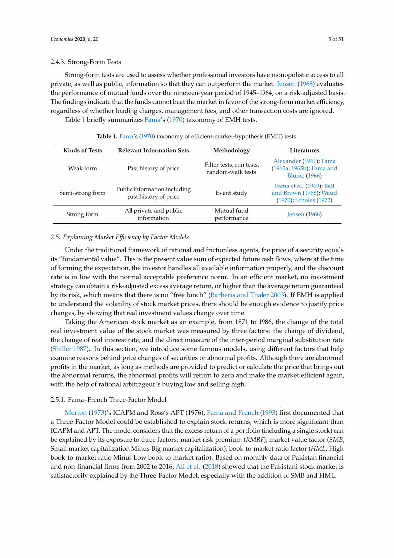
Table 1 briefly summarizes Fama’s (1970) taxonomy of EMH tests.

Table 1. Fama’s (1970) taxonomy of efficient-market-hypothesis (EMH) tests.

Kinds of Tests Relevant Information Sets Methodology Literatures

Weak form Past history of price Filter tests, run tests,random-walk tests

Alexander (1961); Fama(1965a, 1965b); Fama and

Blume (1966)

Semi-strong form Public information includingpast history of price Event study

Fama et al. (1969); Balland Brown (1968); Waud

(1970); Scholes (1972)

Strong form All private and publicinformation

Mutual fundperformance Jensen (1968)

2.5. Explaining Market Efficiency by Factor Models

Under the traditional framework of rational and frictionless agents, the price of a security equalsits “fundamental value”. This is the present value sum of expected future cash flows, where at the timeof forming the expectation, the investor handles all available information properly, and the discountrate is in line with the normal acceptable preference norm. In an efficient market, no investmentstrategy can obtain a risk-adjusted excess average return, or higher than the average return guaranteedby its risk, which means that there is no “free lunch” (Barberis and Thaler 2003). If EMH is appliedto understand the volatility of stock market prices, there should be enough evidence to justify pricechanges, by showing that real investment values change over time.

Taking the American stock market as an example, from 1871 to 1986, the change of the totalreal investment value of the stock market was measured by three factors: the change of dividend,the change of real interest rate, and the direct measure of the inter-period marginal substitution rate(Shiller 1987). In this section, we introduce some famous models, using different factors that helpexamine reasons behind price changes of securities or abnormal profits. Although there are abnormalprofits in the market, as long as methods are provided to predict or calculate the price that brings outthe abnormal returns, the abnormal profits will return to zero and make the market efficient again,with the help of rational arbitrageur’s buying low and selling high.

2.5.1. Fama–French Three-Factor Model

Merton (1973)’s ICAPM and Ross’s APT (1976), Fama and French (1993) first documented thata Three-Factor Model could be established to explain stock returns, which is more significant thanICAPM and APT. The model considers that the excess return of a portfolio (including a single stock) canbe explained by its exposure to three factors: market risk premium (RMRF), market value factor (SMB,Small market capitalization Minus Big market capitalization), book-to-market ratio factor (HML, Highbook-to-market ratio Minus Low book-to-market ratio). Based on monthly data of Pakistan financialand non-financial firms from 2002 to 2016, Ali et al. (2018) showed that the Pakistani stock market issatisfactorily explained by the Three-Factor Model, especially with the addition of SMB and HML.

Economies 2020, 8, 20 6 of 51

2.5.2. Carhart Four-Factor Model

There are limitations in the Fama–French Three-Factor Model, as factors like short-term reversal,medium-term momentum, volatility, skewness, gambling, and others are not considered or included.Based on the Fama–French Three-Factor Model, Carhart (1997) developed an extended version whichincludes a momentum factor for asset pricing in stock markets. The extra consideration is PR1YR,which is the return for the one-year momentum in stock returns. By applying this Four-FactorModel, Carhart (1997) claimed that it helps to explain a significant amount of variations in time series.Furthermore, the high average returns of SMB, HML, and PR1YR indicate that these three factors couldexplain the large cross-sectional variation of the average returns of stock portfolios.

2.5.3. Fama–French Five-Factor Asset-Pricing Model

Although Carhart’s Four-Factor Model helped develop the Fama–French Three-Factor Model,Fama and French (2015) figured out a new augmentation of the Three-Factor Model by consideringprofitability and investment factors, which is called the Five-Factor Asset-Pricing Model, to fix moreanomaly variables that cause problems to the Three-Factor Model. In addition, Fama and French (2015)concluded that the ability of the Five-Factor Model on capturing mean stock returns performs betterthan the Three-Factor Model.

However, the Five-Factor Model did have its drawbacks. For those low mean returns on smallstocks, just like returns of those firms invest heavily regardless of low profitability, it fails to seize, andit was tested in North America, Europe, and Asia-Pacific stock markets by Fama and French (2017).Furthermore, the performance of the model is insensitive to the way in which the factors are defined.With the increase of profitability and investment factors, the value factors of the Three-Factor Modelbecome superfluous for describing the mean return in the samples that Fama and French (2015) test.

2.5.4. Factor Models in Chinese Markets

Given the development of the factor model itself, Fama–French Three-Factor Model remains thebenchmark in US stock markets for many years. Yet many studies copying Fama–French three factorsin China’s A-share market, have not achieved very satisfactory results until Liu et al.’s (2019) Chineseversion Three-Factor Model. Given the strict IPO regulation rules in China’s A share market, whichconsists of the fact that most of the smallest listed firms are targeted as potential, and reflecting thevalue of, shells, in order to develop this model, Liu, Stambaugh and Yuan deleted 30% of stocks atthe bottom to avoid small listed firms whose values are contaminated by shell-values. Furthermore,they use EP (earning-to-price ratio) to replace BM (book-to-market ratio) due to the former capturingthe value effect more accurately in China in the sense that it is the most significant factor.

Using this Chinese version of the Three-Factor Model, most reported anomalies in China’s A-sharemarket are well explained, where profitability and volatility anomalies are included. Furthermore,Liu et al. (2019) add the turnover factor PMO (Pessimistic minus Optimistic) into the model to make ita Four-Factor Model and help explain reversal and turnover anomalies. Same on the studies of Chinastock markets, based on the Fama–French Five-Factor Model, Li et al. (2019) developed a Seven-FactorModel by adding trading volume and turnover rates factors.

When additional factors are included, the Chinese version of the Seven-Factor Model performswell in empirical testing of herding behavior in China’s A-share market, especially during three famousstock market crash periods.

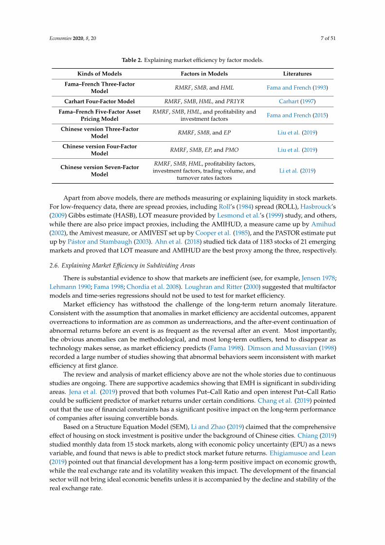
Table 2 briefly summarizes factor models that explain market efficiency.

Economies 2020, 8, 20 7 of 51

Table 2. Explaining market efficiency by factor models.

Kinds of Models Factors in Models Literatures

Fama–French Three-FactorModel RMRF, SMB, and HML Fama and French (1993)

Carhart Four-Factor Model RMRF, SMB, HML, and PR1YR Carhart (1997)

Fama–French Five-Factor AssetPricing Model

RMRF, SMB, HML, and profitability andinvestment factors Fama and French (2015)

Chinese version Three-FactorModel RMRF, SMB, and EP Liu et al. (2019)

Chinese version Four-FactorModel RMRF, SMB, EP, and PMO Liu et al. (2019)

Chinese version Seven-FactorModel

RMRF, SMB, HML, profitability factors,investment factors, trading volume, and

turnover rates factorsLi et al. (2019)

Apart from above models, there are methods measuring or explaining liquidity in stock markets.For low-frequency data, there are spread proxies, including Roll’s (1984) spread (ROLL), Hasbrouck’s(2009) Gibbs estimate (HASB), LOT measure provided by Lesmond et al.’s (1999) study, and others,while there are also price impact proxies, including the AMIHUD, a measure came up by Amihud(2002), the Amivest measure, or AMIVEST set up by Cooper et al. (1985), and the PASTOR estimate putup by Pástor and Stambaugh (2003). Ahn et al. (2018) studied tick data of 1183 stocks of 21 emergingmarkets and proved that LOT measure and AMIHUD are the best proxy among the three, respectively.

2.6. Explaining Market Efficiency in Subdividing Areas

There is substantial evidence to show that markets are inefficient (see, for example, Jensen 1978;Lehmann 1990; Fama 1998; Chordia et al. 2008). Loughran and Ritter (2000) suggested that multifactormodels and time-series regressions should not be used to test for market efficiency.

Market efficiency has withstood the challenge of the long-term return anomaly literature.Consistent with the assumption that anomalies in market efficiency are accidental outcomes, apparentoverreactions to information are as common as underreactions, and the after-event continuation ofabnormal returns before an event is as frequent as the reversal after an event. Most importantly,the obvious anomalies can be methodological, and most long-term outliers, tend to disappear astechnology makes sense, as market efficiency predicts (Fama 1998). Dimson and Mussavian (1998)recorded a large number of studies showing that abnormal behaviors seem inconsistent with marketefficiency at first glance.

The review and analysis of market efficiency above are not the whole stories due to continuousstudies are ongoing. There are supportive academics showing that EMH is significant in subdividingareas. Jena et al. (2019) proved that both volumes Put–Call Ratio and open interest Put–Call Ratiocould be sufficient predictor of market returns under certain conditions. Chang et al. (2019) pointedout that the use of financial constraints has a significant positive impact on the long-term performanceof companies after issuing convertible bonds.

Based on a Structure Equation Model (SEM), Li and Zhao (2019) claimed that the comprehensiveeffect of housing on stock investment is positive under the background of Chinese cities. Chiang (2019)studied monthly data from 15 stock markets, along with economic policy uncertainty (EPU) as a newsvariable, and found that news is able to predict stock market future returns. Ehigiamusoe and Lean(2019) pointed out that financial development has a long-term positive impact on economic growth,while the real exchange rate and its volatility weaken this impact. The development of the financialsector will not bring ideal economic benefits unless it is accompanied by the decline and stability of thereal exchange rate.

Economies 2020, 8, 20 8 of 51

Moreover, in some simulation cases, possibilities are found to help explain market efficiency.For example, in the experiment of Zhang and Li (2019), AR and TAR models with gamma randomerrors were tested on empirical volatility data of 30 stocks, with 33% of them being very suitable,indicating that the model may be a supplement to the current Gaussian random error model withappropriate adaptability. In addition, in some cases, scholars will examine and compare severalmethods on market efficiency explanation, before applicable practical prediction. Guo et al. (2017b)used first-order stochastic dominance and the Omega ratio in market efficiency examination andapplied the theory they put forward to test the relationship between the scale of assets and real-estateinvestment in Hong Kong.

It is possible that scholars will find conflicts again. When studying impacts of exchange rateson stock markets, Ferreira et al. (2019) found that the exchange rate has a significant impact onIndian stock market, while there is no significant impact on European stock market. In the researchof Lee and Baek (2018), although changes in oil prices do have a significant and positive impact onrenewable energy stock prices in an asymmetric manner, it is a short-term impact only. Although insome of the cases, the existing models could not be considered, or quantitative analysis and modelingare still in progress, it is reasonable to postulate that, if the abnormal returns underlying anomalies arewell explained, the market will become efficient with arbitrage.

Many scholars hypothesize that stock prices that are determined in efficient markets cannot becointegrated. Nonetheless, Dwyer and Wallace (1992) showed that market efficiency or the existenceof arbitrage opportunities are not related to cointegration. However, Guo et al. (2017b) developedstatistics that academics and practitioners can use to test whether the market is efficient, whether ornot there are any arbitrage opportunities, and whether there is any anomaly. Stein (2009) examinedwhether the market is efficient by both crowding and leverage factors for sophisticated investors.

Chen et al. (2011) applied cointegration and the error-correction method to obtain aninterdependence relationship between the Dollar/Euro exchange rate and economic fundamentals.They found that both price stickiness and secular growth affect the exchange rate path. Clark et al.(2011) applied stochastic dominance to get efficient portfolio from an inefficient market. By applying astochastic dominance test, Clark et al. (2016) examined the Taiwan stock and futures markets,

Lean et al. (2015) examined the oil spot and futures markets; Qiao and Wong (2015) examinedthe Hong Kong residential property market; and Hoang et al. (2015b) examined the Shanghai goldmarket. Each of these papers concluded that the markets are efficient. However, Tsang et al. (2016)examined the Hong Kong property market by using the rental yield, and concluded that the market isnot efficient and there exist arbitrage opportunities in the Hong Kong property market.

3. Market Anomalies

There are many market anomalies that are important areas of theoretical and practical interestin Behavioral Finance. As many market anomalies have been observed that EMH cannot explain,many academics have to think of a new theory to explain market anomalies found, and this make avery important new area in finance, Behavioral Finance, which can be used to explain many marketanomalies. We discuss some market anomalies in this section and discuss Behavioral Finance in thenext section.

3.1. Winner–Loser Effect/Reversal Effect

De Bondt and Thaler (1985, 1987) found that investors are too pessimistic about the past loserportfolio and too optimistic about the past winner portfolio, resulting in the stock price deviatingfrom its basic value. After a period of time, when the market is automatically correct, past losers arewinning positive excess returns, while past winners are having negative excess returns, which supportthe Winner–Loser Effect. In particular, stocks used in the experiment of De Bondt and Thaler (1985) arethose top 35 and those worst 35 in the long-term (five years period), then a return reversal happens in

Economies 2020, 8, 20 9 of 51

the next three years. Thus, a new method can be advanced to predict stock returns: using reversalstrategy to buy the loser portfolio in the past three to five years and sell the winner portfolio.

This strategy enables investors to obtain excess returns in the next three to five years. Further,Jegadeesh (1990) and Lehmann (1990), respectively, proved that return reversal also happens in theshort-term. The representative heuristic (Tversky and Kahneman 1974), for example, people tend torely too heavily on small samples and rely too little on large samples, inadequately discount for theregression phenomenon, and discount inadequately for selection bias in the generation or reporting ofevidence (Hirshleifer 2001), can be used to explain the Winner–Loser Effect.

Thus, due to the existence of representative heuristics, investors show excessive pessimism aboutthe past loser portfolio and excessive optimism about the past winner portfolio, that is, investorsoverreact to both good news and bad news. This will lead to the undervaluation of the loser portfolioprice and the overvaluation of the winner portfolio price, causing them to deviate from their basic values.

3.2. Momentum Effect

At the moment when more and more empirical evidences are gathered to testify Winner–LoserEffect, Jegadeesh and Titman (1993) found that stock returns are positively correlated in the periodof 3–12 months, i.e., the Momentum Effect. If stock returns are examined over a period of sixmonths, the average return of the “winner portfolio” is about 9% higher than that of the “loserportfolio”. Chan et al. (1996) enlarged Jegadeesh and Titman’s (1993) research samples and obtainedthe same results.

Research conducted by Rouwenhorst (1998) showed that the Momentum Effect also exists in otherdeveloped markets and some emerging stock markets. Moskowitz and Grinblatt (1999) studied theMomentum Effect of portfolio selected by industry, and they found that the industry portfolio hassignificant Momentum Effect in the US stock market, and the abnormal return is larger than that ofindividual portfolio.

Unlike other researchers in the literature, Asness et al. (2014) challenged the existence ofmomentum itself, instead of explaining it by claiming the limitation of momentum. They proved thatmomentum return is small in size, fragmentary, under the concern of disappearing, and only applicablein short position. In the second place, momentum itself is unstable to rely on, behind which there is notheory. Last but not least, momentum might not exist or be limited by taxes or transaction costs, and itprovides various results, depending on different momentum measures in a given period of time.

3.3. Calendar Anomalies—January Effect, Weekend Effect, and Reverse Weekend Effect

3.3.1. January Effect

The January Effect was first discovered by Wachtel (Wachtel). In a further research, Rozeff

and Kinney (1976) found that the return of NYSE’s stock index in January from 1904 to 1974 wassignificantly higher than that of other 11 months. Gultekin and Gultekin (1983) studied the stockreturns of 17 countries from l959 to l979, and found that 13 of them had higher stock returns in Januarythan in other months. Lakonishok et al. (1998) found that, between l926 and l989, the smallest 10%of stock returns exceeded those of other stocks in January. Nippani and Arize (2008) found strongevidence of the January Effect in the study of three major US market indices: corporate bond index,industrial index, and public utility index from, 1982 to 2002. However, according to Riepe (1998),the January Effect is weakening.

The most important explanations for the January Effect are the Tax-Loss Selling Hypothesis(Gultekin and Gultekin 1983) and the Window Effect Hypothesis (Haugen and Lakonishok 1988):the Tax-Loss Selling Hypothesis holds that people will sell down stocks at the end of the year, therebyoffsetting the appreciation of other stocks in that year, in order to achieve the purpose of paying lesstax. After the end of the year, people buy back these stocks. This collective buying and selling leads toa year-end decline in the stock market and a January rise in the stock market the following year.

Economies 2020, 8, 20 10 of 51

The Window Effect Hypothesis holds that institutional investors want to sell losing stocks andbuy profitable stocks to decorate year-end statements. This kind of trading exerts positive pricepressure on profitable stocks at the end of the year, and negative pressure on losing stocks. Whenthe selling behavior of institutional investors stops at the end of the year, the losing stocks that weredepressed in the previous year will rebound tremendously in January, leading to a larger positive trendof income generation.

Sias and Starks (1997), Poterba and Weisbenner (2001), and Chen and Singal (2004) compared andanalyzed the explanatory effect of the Window Effect Hypothesis and Tax-Loss Selling Hypothesis onthe January Effect, and preferred the explanation of Tax-Loss Selling Hypothesis. Starks et al. (2006),based on the above research, through the study of closed-end funds of municipal bonds, further provedthat the Tax-Loss Selling Hypothesis is the real reason for the January Effect.

3.3.2. Weekend Effect and Reverse Weekend Effect

In distinguish or test between the Weekend Effect and Reverse Weekend Effect is easy. When onegets higher returns on Friday than on Monday, it is regarded as the Weekend Effect, and when one getshigher returns on Monday rather on Friday, it is called the Reverse Weekend Effect. Weekend effectshave been identified in the foreign-exchange and money markets, as well as in stock market returnsby many scholars. Based on daily data from 1990 to 2010, in the world, Europe, and other countries,Bampinas et al. (2015) investigated the weekend effect of the Securitization Real Estate Index andconcluded that the average return rate on Friday is significantly higher than that on other days of theweek. Chan and Woo (2012) found the evidence of reverse weekend effect when Monday exhibited thehighest returns for the H-shares index in Hong Kong from 3 January 2000 to 1 August 2008.

However, Olson et al. (2015) examined the US stock market with cointegration analysis andbreakpoint analysis and concluded that, after the discovery of the weekend effect in 1973, the weekendeffect tends to weaken and disappears in the long run. In the United States, although the effect appearsto be stronger in the 1970s than in earlier or later times, there already exist various explanations forstock market behavior on weekends. For example, the regular Weekend Effect has been attributed topayment and check-clearing settlement lags.

Kamstra et al. (2000) claimed that the importance of daylight-saving-time changes indicatedin their paper makes the issue something well worth sleeping on, and a matter that is as worthy offurther study as to other explanations of the weekend anomaly. When the Weekend Effect weakensand disappears, the Reverse Weekend Effect will appear. In the continuous studies of Brusa et al.(2000, 2003, 2005), the Reverse Weekend Effect was found: (1) The main stock indexes have the ReverseWeekend Effect. (2) The Weekend Effect tends to be related to small firms, while the Reverse WeekendEffect tends to be related to large firms. During the period in which Reverse Weekend Effect is observed,the Monday returns of large firms tend to follow the positive Friday returns of last Friday, but they donot follow the negative Friday returns. (3) After 1988, both the broad market index and the industryindex showed positive returns on Monday. Returns were regressed, with Monday as a dummy variable,in Brusa et al.’s (2011) research, and they emphasized that the Reverse Weekend Effect is widelydistributed in large companies, not just a few.

3.4. Book-to-Market Effect/Value Anomaly

Many studies have been undertaken on the Book-to-Market (BM) effect by scholars around theworld. Fama and French (1992) studied all stocks listed in NYSE, AMEX and NASDAQ from 1963to 1990 and found that the combination with the highest BM value (value portfolio) had a monthlyaverage return of 1.53% over the combination with the lowest BM value (charm portfolio). Wang andXu (2004) took A-share stocks in Shanghai and Shenzhen stock markets from June 1993 to June 2002 assamples, calculated the return data of holding one, two, and three years, and considered that the BMeffect exists. The same conclusion was drawn by Lam et al.’s (2019) study covering data from July 1995to June 2015 in Chinese stock markets.

Economies 2020, 8, 20 11 of 51

Black (1993) and MacKinlay (1995) argued that BM effect exists only in a specific sample during aspecific test period, and is the result of data mining, which is not the same as what Kothari et al. (1995)found: It is the selection bias in the formation of BM combination that causes the BM effect. However,Chan et al. (1991), Davis (1994), and Fama and French (1998) tested the stock market outside theUnited States or during the extended test period, and still found that the BM effect existed significantly,negating the argumentation of Black (1993) and MacKinlay (1995).

Fama and French (1992, 1993, 1996) asserted that BM represents a risk factor, i.e., financialdistress risk. Companies with high BM generally have poor performance in profitability, sales, andother fundamental aspects. Their financial situation is also more fragile, making their risk higherthan that of companies with low BM. What is also considered is that the high return obtained bycompanies with high BM is only the compensation for their own high risk, and is not the unexplainedanomaly. Furthermore, for the BM effect on the international level, Fama and French (1998) confirmedthat a Two-Factor Model with a relative distress risk factor added could explain it rather than aninternational CAPM.

De Bondt and Thaler (1987) and Lakonishok et al. (1994) agreed that the BM effect is causedby investors’ overreaction to company fundamentals. On the premise of confirming the positivecorrelation between BM and the company’s fundamentals, as investors are usually too pessimisticabout companies with poor fundamentals and too optimistic about companies with good fundamentals,when the overreaction is corrected, the profits of high BM companies will be higher than those of lowBM companies.

3.5. The Size Effect

Banz (1981) found that the stock market value decreased with the increase of company size.The phenomenon that small-cap stocks earn higher returns than those calculated by CAPM (Reinganum1981) and large-cap stocks (Siegel 1998) clearly contradicts EMH especially in January, as size of thefirm and arrival of January are regarded as public information. Lakonishok et al. (1994) found that,since the stock with high P/E ratio is riskier, if P/E ratio is presumed to be known information, then thisnegative relationship between P/E ratio and return rate provides a considerable prediction on the latter,bringing a serious challenge to EMH.

On the contrary, Daniel and Titman (1997) claimed that BM and size only represent the preferenceof investors, not the determinants of returns. Due to the poor fundamentals of high BM companiesand good fundamentals of low BM companies, while investors prefer to hold value stocks with goodfundamentals rather than those with poor fundamentals, the return rate of companies with high BMis higher.

3.6. Disposition Effect

Shefrin and Statman (1985) proposed that the Disposition Effect refers to two phenomena of thestock market: The first is that investors tend to have a strong psychology of holding loss-making stocksand are not willing to realize losses; and the second is that investors tend to avoid risks before profits,thereby willing to sell stocks in order to lock in profits. In these cases, two kinds of psychology are addedto describe investors where regret and embarrassment cause the first phenomenon, and arroganceleads to the second.

The Disposition Effect is one implication of extending Kahneman and Tversky’s prospect theory(1979) to investments. For example, suppose an investor purchases a stock that she believes to have anexpected return high enough to justify its risk. If the stock appreciates and she continues to use thepurchase price as a reference point, the stock price will then be in a more concave, risk-averse part of theinvestor’s value function. The stock’s expected return may continue to justify its risk, but if the investorlowers her expectation for the stock’s return somewhat, she will be likely to sell the stock. If instead ofappreciating, the stock declines, its price is in the convex, risk-seeking part of the value function.

Economies 2020, 8, 20 12 of 51

Consequently, the investor will continue to hold the stock even if its expected return falls lowerthan would have been necessary for her to justify its original purchase. Thus, the investor’s beliefabout expected return must fall further, to motivate the sale of a stock that has already declined ratherthan one that has appreciated. Similarly, suppose an investor holds two stocks. One is up, and theother is down. If he is facing a liquidity demand and has no new information about either stock, he ismore likely to sell the stock that is up (Barber and Odean 1999).

In addition, Kahneman and Tversky (1979) argued that investors are more concerned with regretthan arrogance, and therefore are more willing to take no action, which leads investors to be reluctantto lose or make a profit, while those who do not sell profitable shares worry that prices will continue torise. In other words, if one investor is not confident enough in trading stocks, he or she tends to followinvestment advisers’ decision or advice to buy or sell a stock, which, at least, no matter the selectedstock gains or losses, he or she is not the one to be blamed and thus reduces the feeling of regret.

Locke and Mann (2015) provided evidence that professional futures floor traders appear tobe subject to Disposition Effect. These traders as a group hold losing trades longer on averagethan gains. Their evidence also indicates that relative aversion to loss realization is related tocontemporaneous and future trader relative success. Though many factors can coordinate trading (e.g.,tax-loss selling, rebalancing, changing risk preference, or superior information), Barber et al. (2005)argued their empirical results are primarily driven by three behavioral factors: the representativenessheuristic, limited attention, and the disposition. When buying, similar beliefs about performancepersistence in individual stocks may lead investors to buy the same stocks—a manifestation of therepresentativeness heuristic.

Investors may also buy the same stocks simply because those stocks catch their attention.In contrast, when selling, the extrapolation of past performance and attention play a secondaryrole. Attention is less of an issue for selling, since most investors refrain from short selling and caneasily give attention to the few stocks they own. If investors solely extrapolated past performance,they would sell losers. However, they do not. This is because, when selling, there is a powerfulcountervailing factor—the Disposition Effect—a desire to avoid the regret associated with the sale of alosing investment. Thus, investors sell winners rather than losers.

Barber et al. (2008) analyzed all trades made on the Taiwan Stock Exchange between 1995 and1999 and provided strong evidence that, in aggregate and individually, investors have a DispositionEffect; that is, investors prefer to sell winners and hold losers. The Disposition Effect exists for bothlong and short position, for both men and women (to roughly the same degree), and tends to declinefollowing periods of market appreciation.

Odean (1998a, 1999) proposed an indicator to measure the degree of Disposition Effect andused this indicator to verify the strong selling, earning, and losing tendency of US stock investors.Meanwhile, Odean also found that US stock investors sold more loss-making shares in December,making the effect less pronounced because of tax avoidance. In the research on the DispositionEffect of the Chinese stock market, Zhao and Wang (2001) concluded that Chinese investors are moreinclined to sell profitable stocks and continue to hold loss-making stocks, which is more serious thanforeign investors.

3.7. Equity Premium Puzzle

The Equity Premium Puzzle, first proposed by Mehra and Prescott (1985), refers to the fact thatequity yields far exceed Treasury yields. Rubinstein (1976) and Lucas (1978) showed that the stockpremium could only be explained by a very high-risk aversion coefficient. Kandel and Stambaugh(1991) argued that risk aversion is actually higher than traditionally thought. However, this leadsto the risk-free interest rate puzzle of Weil (1989): In order to adapt to the low real interest rate,they observed, investors can only be assumed to give preference weights equal to or higher than theircurrent consumption in the future. This results in low or even a negative time preference rate ofinvestors where, in practice, negative time preferences are impossible.

Economies 2020, 8, 20 13 of 51

In order to solve the risk-free interest rate puzzle suggested by Weil (1989), Epstein and Zin (1991)further introduced the utility function of investors’ first-level risk aversion attitude, which is unrelatedto the risk-aversion coefficient and the cross-time substitution elasticity of consumers. With generalizedexpected utility proposed, this model solves the risk-free interest rate puzzle rather than the equitypremium. At the same time, more and more revised versions of the utility function occur: a utilityfunction containing the past consumer spending habits’ effect shows that equity premium is due toindividuals being more sensitive to the shrinking of short-term consumption (Constantinides 1990).

The consumption utility function, affected by the average consumption level of the society,is defined to explain the risk-free interest rate puzzle to a certain extent from the demand for bonds(Abel 1990). Studies that explain the Equity Premium Puzzle under certain economic conditions,apart from the catastrophic event with low probability, as studied by Rietz (1988), will increase thestock premium. In the research of Berkman et al. (2017), the expected market risk premium wassuccessfully explained by using a measure of global political instability as an indicator of disaster risk,a profit–price ratio, and a dividend–price ratio, respectively.

Campbell and Cochrane (1999), adding the probability of the recession which will lead to futureconsumption levels included in the utility function, concluded the following: The increase in theprobability, on the one hand, can lead to investor risk aversion increases, so they prefer a higher riskpremium; on the other hand, this will increase the investor demand to meet the motives of prevention,so that the risk-free interest rate will fall.

Cecchetti et al. (2000) proposed an irrational expectation method to explain the equity premium bycomparing it with the rational expectations of Campbell and Cochrane (1999). Chen (2017) explainedthat the Equity Premium Puzzle is due to habits formed during the life cycle of the economy, especiallyduring recessions; for example, households develop a habit of maintaining comfortable lifestyles,which leads to macroeconomic risks that are not reflected in asset-pricing models. Not until 2019, in amodel that uses age-dependent increased risk aversion but no other illogical levels of risk aversionassumptions, did DaSilva et al. (2019) obtain results consistent with US equity premium data.

In terms of the risk of labor income, which will produce losses, Heaton and Lucas (1996, 1997)claimed that investors require higher equity premium as compensations, so that they are willing tohold stocks, then generating equity premium. However, Constantinides and Duffie (1996) arguedthat the corresponding situation happens at a time of economic depression, when investors are morereluctant to hold stocks, for the fear of decline in the value of their equity assets; thus, higher equitypremium is necessary to attract investors.

Kogan et al. (2007) found out that equity premium could be achieved in an economy that imposesborrowing constraints, while Constantinides et al. (2002) noted that equity premium is determinedby middle-aged investors under the conditions of relaxed lending constraints. Bansal and Coleman(1996) claimed that negative liquidity premium of bonds reduces the risk-free interest rate and furtherexpands the gap with stock returns, causing the Equity Premium Puzzle.

De Long et al. (1990) claimed that dividend generation is a high-risk process that leads to a highequity premium. Lacina et al. (2018) got rid of the use of the way forecasts, proving a near-zerorisk premium. In addition, individual income tax rates (McGrattan and Prescott 2010), GDP growth(Faugere and Erlach 2006), and information (Gollier and Schlee 2011; Avdisa and Wachter 2017) andspatial dominance (Lee et al. 2015) are also used to explain the Equity Premium Puzzle.

With the rise of Behavioral Finance, some scholars began to use theories from Behavioral Financeto explain the Equity Premium Puzzle. Benartzi and Thaler (1995) proposed a causal relationshipbetween loss aversion and equity premium based on prospect theory: Precisely due to the fact thatinvestors are afraid of stock losses, equity premium is an important factor to attract investors to holdstock assets and maintain the proportion of stocks and bonds in their portfolios.

Furthermore, Barberis et al. (2001) emphasized in the BHS model they constructed that investors’loss aversion would constantly change, thus generating equity premium, while Ang et al. (2005),Xie et al. (2016), and others explained the Equity Premium Puzzle by introducing disappointment

Economies 2020, 8, 20 14 of 51

aversion of Behavioral Finance as an influence factor. Hamelin and Pfiffelmann (2015) used BehavioralFinance to explain why entrepreneurs who are aware of their high exposure still accept low returnsand show the cognitive traders the riddle of how to explain the private equity.

Mehra and Prescott (2003) analyzed 107 papers on the research of the Equity Premium Puzzle,and drew a conclusion that none has provided a plausible explanation. Given the above reviewin this paper, a conclusion can be drawn that, with the existing and unsolved anomalies in stockmarkets, efficiency in stock markets requires certain assumptions. In other words, on the way tosolve and explain anomalies, a large number of models will be set up, along with new assumptionsinside those models. Many long-standing puzzles can already be solved with different techniques(Ravi 2018), though extra efforts need to be paid on academic research as the world grows quicker withtechnological developments, making economics complicated.

3.8. Herd Effect and Ostrich Effect

Patel et al. (1991) introduced two behavioral hypotheses to help explain financial phenomena:Barn Door Closing for mutual fund purchases and Herd Migration Behavior for debt–equity ratio.Barn Door Closing, in the horse protection sense, refers to undertaking behavior today that wouldhave been profitable yesterday. Herd Migration in finance occurs when market conditions change,so that individual decision makers wish to alter their holdings substantially.

Their transition is slowed because they seek protection by traveling with the herd. Herd behavior(i.e., people will do what others are doing rather than what is optimal, given their own information)refers to behavior patterns that are correlated across individuals—but could also be caused by correlatedinformation arrival in independently acting investors.

Herding is closely linked to impact expectations, fickle changes without new information, bubbles,fads, and frenzies. Barber et al. (2003) compared the investment decisions of groups (stock clubs)and individuals. Both individuals and clubs are more likely to purchase stocks that are associatedwith good reasons (e.g., a company that is featured on a list of most-admired companies). However,stock clubs favor such stocks more than individuals, despite the fact that such reasons do not improveperformance. The mentioned Seven-Factor Model by Li et al. (2019) also indicates that herd behavior ofChinese A-share market is more prevalent in times of market turmoil, especially when the market falls.

Hon (2015b) found a significant correlation between the reason given by small investors forchanging their current security holdings, and the reason given for the sharp correction in the bankstock market. This empirical finding suggests that herding behavior occurred frequently among thesmall investors, and they tend to sell their stock during the sharp correction period. Hon (2013d)found that there was a change in the behavior of small investors during and immediately after thebuoyant stock market of January 2006 to October 2007, in Hong Kong. During the buoyant market,small investors were overconfident and bought stock. The small investors also exhibit herd behavior,and, once the sharp correction to the market began after October 2007, they sold the stock.

In Galai and Sade (2006)’s paper, it is recorded that government Treasury bonds provide highermaturity rates than non-current assets with the same risk level in Israel. Additional research showsthat liquidity is positively correlated with market information flows. As ostriches are thought to dealwith obvious risk situations by hopefully pretending that risk does not exist, so the ostrich effect isused to describe the above investors’ behavior. Karlsson et al. (2009) presented a decision theoreticalmodel in which information collection is linked to investor psychology.

For a wide range of plausible parameter values, the model predicts that the investor should collectadditional information conditional on favorable news, and avoid information following bad news.Empirical evidence collected from Scandinavian investors supports the existence of the ostrich effect infinancial markets.

Economies 2020, 8, 20 15 of 51

3.9. Bubbles

The first study to report bubbles in experimental asset markets was published by Smith et al.(1988). Bubbles feature large and rapid price increases which result in the rising of share prices tounrealistically high levels. Bubbles typically begin with a justifiable rise in stock prices. The justificationmay be a technological advance or a general rise in prosperity. The rise in share prices, if substantialand prolonged, leads to members of the public believing that prices will continue to rise.

People who do not normally invest begin to buy shares in the belief that prices will continueto rise. More and more people, typically those who have no knowledge of financial markets, buyshares. This pushes up prices even further. There is euphoria and manic buying. This causes furtherprice rises.

There is a self-fulfilling prophecy wherein the belief that prices will rise brings about the rise,since it leads to buying. People with no knowledge of investment often believe that if share prices haverisen recently, those prices will continue to rise in the future (Redhead 2003). A speculative bubblecan be described as a situation in which temporarily high prices are sustained largely by investors’enthusiasm rather than by consistent estimations of real value. The essence of a speculative bubble isa sort of feedback, from price increases to increased investor enthusiasm, to increased demand, andhence further price increases. According to the adaptive expectations’ version of the feedback theory,feedback takes place because past price increases generate expectations of further price increases.

According to an alternative version, feedback occurs as a consequence of increased investorconfidence in response to past price increases. A speculative bubble is not indefinitely sustainable.Prices cannot go up forever, and when price increases end, the increased demand that the priceincreases generated ends. A downward feedback may replace the upward feedback.

Shiller’s (2000) paper presents evidence on two types of investor attitudes that change in importantways through time, with important consequences for speculative markets. The paper explores changesin bubble expectations and investor confidence among institutional investors in the US stock market atsix-month intervals for the period 1989 to 1998 and for individual investors at the start and end ofthis period.

Since current owners believe that they can resell the asset at an even higher price in the future,bubbles refer to asset prices that exceed an asset’s fundamental value. There are four main strands ofmodels that identify conditions under which bubbles can exist.

The first class of models assumes that all investors have rational expectations and identicalinformation. These models generate the testable implication that bubbles have to follow an explosivepath. In the second category of models, investors are asymmetrically informed and bubbles can emergeunder more general conditions because their existence need not be commonly known.

A third strand of models focuses on the interaction between rational and behavioral traders.Bubbles can persist in these models since limits to arbitrage prevent rational investors from eradicatingthe price impact of behavioral traders.

In the final class of models, bubbles can emerge if investors hold heterogeneous beliefs, potentiallydue to psychological biases, and they agree to disagree about the fundamental value. Experiments areuseful to isolate, distinguish, and test the validity of different mechanisms that can lead to or rule outbubbles (Abreu and Brunnermeier 2003).

West (1987) suggested that the set of parameters needed to calculate the expected presentdiscounted value of a stream of dividend can be estimated in two ways. One may test for speculativebubbles, or fads, by testing whether the two estimates are the same. When the test is applied to someannual US stock market data, the data usually reject the null hypothesis of no bubbles. The test isgenerally interesting, since it may be applied to a wide class of linear rational expectations models.The seeming tendency for self-fulfilling rumors about potential stock price fluctuations to result inactual stock price movements has long been noted by economists.

For example, in a famous passage, Keynes describes the stock market as a certain type of beautycontest: speculators devote their “intelligence to anticipating what average opinion expects average

Economies 2020, 8, 20 16 of 51

opinion to be”. In recent rational expectations’ work, this possibility has been rigorously formalized,and the self-fulfilling rumors have been dubbed speculative bubbles.

Craine (1993) suggests that the fundamental value of a stock is the sum of the expected discounteddividend sequence. Bubbles are deviations in the stock’s price from the fundamental value. Rationalbubbles satisfy an equilibrium pricing restriction, implying that agents expect them to grow fast enoughto earn the expected rate of return. The explosive growth causes the stock’s price to diverge from itsfundamental value.

Whether the actual volatility of equity returns is due to time variation in the rational equityrisk premium or to bubbles, fads, and market inefficiencies is an open issue. Bubble tests require awell-specified model of equilibrium expected returns that have yet to be developed, and this makesinference about bubbles quite tenuous.

Chan and Woo (2008) employed a new test to detect the existence of stochastic explosive rootbubbles. If a speculative bubble exists, the residual process from the regression of stock prices ondividends will not be stationary. The data series include the monthly aggregate stock price indices,dividend yields and price indices for the stock markets of Taiwan, Malaysia, Indonesia, the Philippines,Thailand, and South Korea. The sample period spans from March 1991 to October 2005 for all markets.

The dividend series are estimated by multiplying the price indices by dividend yields. The stockprice indices and dividends are deflated by the producer price index for Malaysia, and by the consumerprice indices for the other markets. They found evidence of bubble in stock markets of Taiwan,Malaysia, Indonesia, the Philippines and Thailand, but no evidence of bubbles in South Korea overtheir sample period.

Homm and Breitung (2012) proposed several reasonable bubble-testing methods, which areapplied to NASDAQ index and other financial time series, to test their power properties, coveringchanges from random walk to explosion process. They concluded that a Chow-type break test providesthe highest power and performs well relative to the power envelope, and they also put forward aprogram to monitor speculative bubbles in real time.

In order to explore bubbles further, in the next section, we introduce several factors underlyingthe bubble that help explain bubbles.

3.9.1. The Internet

Investors, in general, and online investors, in particular, now make decisions in a very differentenvironment than investors in the past. They have access to far more data via the Internet. They oftenact without personal intermediaries. They can conduct extensive searches and comparisons on a widevariety of criteria. A critical and largely unexplored research question is how this different environmentaffects the decision-making of investors (Barber and Odean 2001b).

Barber and Odean (2002) analyzed 1607 investors who switched from phone-based to onlinetrading during the 1990s. Those who switched to online trading performed well prior to goingonline, beating the market by more than 2% annually. After going online, they traded more actively,more speculatively, and less profitably than before, lagging the market by more than 3% annually.

Reductions in market frictions (lower trading costs, improved execution speed, and greater easeof access) do not explain these findings. Overconfidence—augmented by self-attribution bias and theillusions of knowledge and control—can explain the increase in trading and reduction in performanceof online investors.

3.9.2. Derivatives

Hon (2013a) attempted to identify the ways that the Hong Kong companies in the Hang SengIndex Constituent Stocks manage their financial risk with derivatives. By analyzing the companies’annual reports and financial reviews, it was found that 82.6% of these companies used derivativesin 2010. Specifically, 58.7% of them used swaps to hedge interest rate risk, and 54.3% of them used

Economies 2020, 8, 20 17 of 51

forward contracts to hedge foreign-exchange risk. The results are largely consistent with the predictionthat companies use derivatives to manage their financial risk.

By investing in stocks, bonds, and other financial assets, people have been able to build up a bufferin case of being dismissed. Firms have tilted their compensation packages to management away fromfixed salaries toward participation and result-based compensations, such as stock options. With suchoptions, management has an incentive to do everything possible to boost share prices. They have anincentive to maintain an appearance of corporate success and a corporation working its way toward animpressive future with increasing profits. It seems as a strategy to boost the stock value and to refinethe company’s objectives and announcing that it was a part of the e-business society.

Heath et al. (1999) investigated stock-option-exercise decisions by over 50,000 employees at sevencorporations. Controlling for economic factors, psychological factors influence exercise. Consistentwith psychological models of beliefs, employee exercise in response to stock price trends—exerciseis positively related to stock returns during the preceding month and negatively related to returnsover longer horizons. Consistent with psychological models of values that include reference points,employee exercise activity roughly doubles when the stock price exceeds the maximum price attainedduring the previous year. Options have no purchase price to serve as a reference point.

Employees do not purchase options; they receive them at a strike price that is equal to the stockprice on the date of the grant. Because employees can only exercise their options when the stock priceexceeds the strike price, reference points, if they exist, will be dynamically determined by stock pricemovement after the grant.

CEO compensation has grown dramatically. Average CEO compensation as a multiple of averageworker compensation rose from 45 in 1980, to 96 in 1990, and to an astounding 458 in 2000. A largeportion of this compensation comes in the form of stock options. Economists fear that managers willbehave more conservatively than is in the best interests of shareholders because managers’ careers aretied to the firm. Executive stock options mitigate this problem by rewarding managers when the firm’sshare price goes up but not punishing them when it goes down. Such convex compensation contractsencourage managers to take risks.

Gervais et al. (2011) argued that executives are likely to be overconfident and optimistic, and thusbiased, when assessing projects, and that many shareholders are under-diversified and do care aboutspecific risk. A manager may further manipulate investor expectations by managing earnings throughdiscretionary accounting choices. Furthermore, research indicates that earnings manipulations canaffect prices.

Derivatives are a new segment of secondary market operations in India. Ganesan et al. (2004)found that a buoyant and supporting cash market is a must for a robust derivative market. Hon’s (2015a)found that the majority of respondents who invested in their derivative investments during January2013 to January 2014 in Hong Kong were relatively younger. More than 58.1% of the respondents hadtertiary education for their derivatives investments. Males preferred to invest in warrants more thanfemales did, while females preferred to invest in stock options more than males did.

Hon (2015c), based on the survey results, derived the ascending order of importance of referencegroup, return performance, and personal background (reference group is the least important andpersonal background is the most important) in the Hong Kong derivatives markets. The results ofHon’s paper (Hon 2013c) indicate that small investors mostly tend to trade Callable Bull/Bear Contacts(35% of total) and warrants (23% of total). Hon (2012) identified five factors that capture the behavior ofsmall investors in derivatives markets in Hong Kong. The factors are personal background, referencegroup, return performance, risk tolerance, and cognitive style.

3.9.3. Feedback Models

The essence of a speculative bubble is the familiar feedback pattern—from price increases toincreased investor enthusiasm to increased demand and, hence, to further price increase. The higher

Economies 2020, 8, 20 18 of 51

demand for the asset is generated by the public’s memory of high past returns and optimism the highreturns generate for the future (Shiller 2002).

When speculative prices go up, creating successes for some investors, this may attract publicattention, promote word-of-mouth enthusiasm, and heighten expectations for further price increases.The talk attracts attention that justifies the price increases. This process, in turn, increases investordemand and thus generates another round of price increases. If the feedback is not interrupted,it may produce after many rounds a speculative “bubble”, in which high expectations for further priceincreases support very high current prices. The high prices are ultimately not sustainable, since theyare high only because of expectations of further price increases, and so the bubble eventually bursts,and prices come falling down.

The feedback that propelled that bubble carries the seeds of its own destruction, and the endof the bubble may be unrelated to news stories about fundamentals. The same feedback mayalso produce a negative bubble, downward price movements propelling further downward pricemovements, promoting word-of-mouth pessimism, until the market reaches an unsustainably lowlevel (Shiller 2003).

3.9.4. Smart Money

The efficient markets theory, as it is commonly expressed, asserts that when irrational optimistsbuy a stock, smart money sells, and when irrational pessimists sell a stock, smart money buys, therebyeliminating the effect of the irrational traders on market price. From a theoretical point of view, it is farfrom clear that smart money has the power to drive market prices to fundamental values. For example,in one model with both feedback traders and smart money, the smart money tended to amplify, ratherthan diminish, the effect of feedback traders, by buying in ahead of the feedback traders in anticipationof price increases they would cause (Shiller 2003). In addition to search costs, investors might choosemutual funds with high expenses if high-expense funds provided better service than other funds.

Barber et al. (2005) asserted that different levels of service are unlikely to explain their results,since first-rate service and low expenses are not mutually exclusive. For example, Vanguard, which iswell-known for its low-cost mutual fund offerings, has won numerous service awards. Barber andOdean (2003) concluded that either models of optimal asset location are incomplete or a substantialfraction of investors are misallocating their assets. Though tax considerations leave clear footprints inthe data they analyzed, many households could improve their after-tax performance by fully exploitingthe tax-avoidance strategies available on equities.

3.9.5. The Media

Media may well have an important role in directing this public attention toward markets, whichmay consequently result in abnormal market behavior. Stock-market price increases generate newsstories, which generate further stories about new-era theories that explain the price increases, which,in turn, generate more news stories about the price increases (Shiller 2002). In the United Kingdom,Diacon (2004) found that lay investors perceive higher risks in investing in financial services productsthan do their financial advisers (coupled with an inherent optimism about likely benefits) has substantialramifications in the light of recent reports, such as the “Sandler Review”. This may have the effect ofencouraging consumers to deal directly with providers rather than via independent financial advisers.

Dispensing with the services of financial advisers is likely to lead consumers to make moreconservative investment choices: for example, by investing too little in equities and too much infixed-income assets when saving retirement. As a result, consumers may find themselves withsurprisingly inadequate levels of savings to meet future commitments such as a pension on retirement.Hon (2013b) studied the investment attitude and behavior of the small investors on derivatives marketsin Hong Kong. He found that the most decisive factor that could influence small investor’s decisionmaking is highly accessible and updated. In total, 37.8% and 25.8% of respondents considered theInternet and news/magazines/newspaper, respectively, as the decisive factor.

Economies 2020, 8, 20 19 of 51

3.9.6. Emotions and Sentiments

There are serious questions concerning whether the phenomenon on excess volatility exists in thefirst place and, and if it does, whether abandonment of assumptions of rational expectations in favor ofassumptions of mass psychology and fads as primary determinants of price changes is the best avenuefor current research (Kleidon 1986). Using common sense, one knows that the stock market couldrepeat the performance of recent years. That possibility seems quite real, just as real as the possibilityof a major correction in the market. The question is how the private investor feels when he fills out hischoice of mutual funds for his retirement scheme. How this person feels depends on his experiencesin investing.

If one has been out of the market without participating in earning money that other investors mayhave done, one may be feeling a sharp pain of regret. Regret has been found by psychologists to be oneof the strongest motivations to make a change in something. Envy is another dominant characteristic:To see other people having made more money in the stock market than oneself has made from work isa painful experience, especially since it diminishes one’s ego. In case the other people were smarter,one feels like a fool, and even if they were not any smarter, just lucky, it may not feel any better.

A common feeling in this situation is that if one can participate just one more year in rising stockmarket everything will be much better and mitigate the pain. One may also think that the potential losswill be much more diminishing to one’s ego than the failure to participate has already been. One mayalso realize that one takes the risk of entering the market just as it begins a downward turn. However,the psychological cost of such a potential future loss may not be so much greater relative to the veryreal regret of having been out of the market in the past.

Barberis et al. (1998) presented a parsimonious model of investor sentiment, or of how investorsform expectations of future earnings. The model they proposed was motivated by a variety ofpsychological evidence; in making forecasts, people pay too much attention to the strength of theevidence they are presented with and too little attention to its statistical weight. Loewenstein et al.(2001) proposed an alternative theoretical perspective, the risk-as-feelings hypothesis, which highlightsthe role of affect experienced at the precise moment of decision-making. Drawing on research fromclinical, physiological, and other subfield of psychology, they showed that emotional reactions to riskysituations often diverge from cognitive assessments of those risks. When such divergence occurs,emotional reactions often drive behavior. The risk-as-feelings hypothesis is shown to explain a widerange of phenomena that have resisted interpretation in cognitive–consequentialist terms.

If one participates in the market today for a while and ponders whether get out or not, he hasa fundamentally different emotional frame of mind. This person feels satisfaction and probablypride in his past successes, and he will certainly feel wealthier. One may feel as gamblers do afterthey have “hit big-time”, i.e., that one is gambling with the “house money”, and therefore hasnothing to lose emotionally by wagering again. The concept of gambling with the house money is atheory about people’s risk preferences and is related to mental accounting. Investors will generallybecome more risk-averse in the case of prior losses and less risk-averse in the case of prior gain(Barberis and Thaler 2003); they will also take greater risks as their profits grow.

This provides support for the notion that successful traders are more likely to be overconfident.The emotional state of investors when they decide on their investment is no doubt one of themost important factors causing bull market. From the neuroscience literature, Peterson (2002)demonstrated correlations between reward anticipation and the arousal of affect (feelings, emotions,moods, attitudes, and preferences). He briefly outlined an investment strategy for exploiting theevent-related security-price pattern described by the trading strategy “buy on the rumor and sell onthe news”.

In their research, Chow et al. (2015) conducted a survey to examine whether the theory developedin Lam et al. (2010, 2012) and Guo et al. (2017a) holds empirically, by studying the behavior of differenttypes of Hong Kong small investors in their investment, especially during financial crisis. They foundthat determinants of the Hong Kong small investors’ investment decision have uniform views as to the

Economies 2020, 8, 20 20 of 51

ascending order of importance of time horizon, sentiment, and risk tolerance. Time horizon is the leastimportant factor, and risk tolerance is the most important factor.

3.10. Volume and Volatility

Fong and Wong (2007) applied the volatility–volume regressions to the daily realized volatility ofcommon stocks to study sources of volatility predictability. They found that unexpected volume canexplain half of the variations in realized volatility and that the ARCH effect is robust in the presenceof volume.

Xiao et al. (2009) studied the relationship between volume and volatility in the entire AustralianStock Market for different firm size and trading volume. They found that daily trading volume hassignificant explanatory power on the variance of daily returns. Actively traded stocks having a largernumber of information arrivals per day will have a larger impact of volume on the variance of dailyreturns. Low trading volume and small firm lead to a higher persistence of GARCH effects, unlikethe elimination effect for the top most active stocks. In general, the elimination of both ARCH andGARCH effects by introducing the volume variable on all other stocks, on average, is not as much asthat for the top most active stocks. The elimination of both ARCH and GARCH effects by introducingthe volume variable is higher for stocks in the largest volume and/or the largest market capitalizationquartile group. Their empirical findings rejected the pure random-walk hypothesis for stock returns,and they concluded that the relationship between volume and volatility is not a statistical fluke. Unlikemost anomalies, the volume effect on volatility is not likely to be eliminated after its discovery.

3.11. Trading Rules and Technical Analysis

If investors could make significant profit when they use any tool in technical analysis, adopt anytrading rule, or employ any indicator in their investment, then we will consider this is an anomalybecause this shows that the market is not efficient so that investors could have opportunity to makeprofit. There are many studies in this area. We list a few here.

We first discuss the adaptation of indicators and trading rules. For instance, Wong et al. (2001)introduced a new stock market indicator by using both E/P ratios and bond yields, and developed twostatistics to test the following hypotheses:

Hypothesis 1 (H1). Using the proposed indicator could make significantly good profit from the markets.

Hypothesis 2 (H2). Using the proposed indicator could beat the buy-and-hold (BH) strategy.

In order to test the hypotheses, they examined the performance of their proposed indicator infive different stock markets, namely the UK, USA, Japan, Germany, and Singapore stock markets.Firstly, from their empirical study, they did not reject the hypothesis H1 in (i) and concluded that theirindicator could produce buy and sell signals that investors could escape from most, if not all, of themajor crashes, catch many of the bull markets, and generate significantly good profit.

Thereafter, they conducted an analysis to test the hypothesis H2 in (ii), and their analysis led themnot to reject the hypothesis in (ii) and to conclude that their proposed indicator performs better thanthe BH strategy, because using their proposed indicator enabled investors to make significant higherprofit then the BH strategy.

McAleer et al. (2016) developed some new indicators, or new trading rules, that can profiteerfrom any main financial crisis, and they examined the applicability of their proposed indicators/tradingrules on the 1997 Asian Financial Crisis (AFC), the 2000 dot-com crisis (DCC), and the 2007 GlobalFinancial Crisis (GFC). They examined the two hypotheses H1 and H2 in (i) and (ii) with theirproposed indicators.

The empirical study did not reject (i) and concluded that using the signals generated by theirproposed indicators/trading rules generate significantly good profit from the markets during AFC,

Economies 2020, 8, 20 21 of 51

DCC, and GFC. Their empirical study also did not reject (ii), and they concluded that their proposedindicators/trading rules beat the BH strategy, because by using their proposed indicators/trading rules,investors could make very huge profit from the markets during AFC, DCC, and GFC; nonetheless,by adopting the BH strategy, all the profits are eaten up by the downtrend of the crisis and investorsend up not having any profit or even bear big loss.

Chong et al. (2017) developed a new market sentiment index by using HIBOR, short-selling volume,money flow, the turnover ratio, the US and Japanese stock indices, and the Shanghai and ShenzhenComposite indices. Thereafter, they used the index as a threshold variable to determine different statesin the market and applied the threshold regression to generate buy-and-sell signals. They illustratedthe applicability of their proposed trading rules on the HSI or S&P/HKEx LargeCapIndex by testing thetwo hypotheses H1 and H2 in (i) and (ii), with the now-proposed indicator as their proposed approach.

Their empirical study did not reject (i), and they concluded that the use of their proposed approachgenerated significant profit from the Hong Kong market; the study did not reject (ii), and it concludedthat their proposed approaches beat the BH strategy when investors buy the stock indices when thesentiment index is smaller than the lower threshold value, and vice versa.

Using both intraday and daily data, Lam et al. (2007) examined both surges and plummets ofstock price and construct momentums and five trading rules of trading in stocks. They found that alltheir proposed trading rules cannot get any significant profit in both European and American stockmarkets but can get significant profit from the Asian stock markets. Their findings accept market forEuropean and American stock markets but reject efficiency in the Asian stock markets, implying thatthe Asian stock markets are not as efficient as American and European stock markets.

There are many trading rules. An easy one is the single lump-sum investment rule (LS) that oneinvests all the fund at the beginning. Another popular one is the dollar-cost averaging investmentrule (DCA) in which, regardless of ups and downs in the markets, one invests a fixed amount ofmoney periodically over a given time interval in equal installments. This approach could avoid riskand the devastating effect when the market crashes suddenly. The literature shows that the LS ruleoutperforms the DCA rule when the market is uptrend, and the DCA rule outperforms the LS rulewhen the market is downtrend or mean-reverted.

Does the LS rule really outperform the DCA rule when the market is uptrend? Lu et al. (2020)conjectured that the DCA rule could still outperform the LS rule when the market is uptrend. To showthat their conjecture could hold true, they applied both Sharpe Ratio (SR) and economic performancemeasure (EPM) and compared the performance of both LS and DCA rules in both accumulative anddisaccumulative situations. They showed that, when the trend is not too upward, the DCA ruleperforms better than the LS rule in almost all the situations. In addition, when the market is uptrend,the DCA rule could still outperforms the LS rule in many situations, especially when volatility is highand when longer investment horizon is chosen.

Thus, the authors concluded that their conjecture hold true that the DCA rule could outperformthe LS rule in many situations even in the situation the market is in the uptrend. Together with thefindings in the literature that the DCA rule outperforms the LS rule when the market is downtrend ormean-reverted, the authors recommended that investors not choose the LS rule but use the DCA rulein their investment.

We note that one could apply the rules in the above papers to make good profit in their studyingperiods. If this is the case, then we will consider this is an anomaly, because this shows that the marketis not efficient so that investors could have opportunity to make profit. However, there is a chance thatthe rules may not be able to make money after the rules released. If this is the case, then the market isstill efficient and the anomaly disappears. Now, we turn to discuss using technical analysis (TA) togenerate profit.

There are many studies that show that technical analysis can be used to generate profit.For example, to examine whether TA is profitable, Wong et al. (2003) used two popular technicaltools—moving average (MA) and relative strength index (RSI)—and introduced two statistics to test

Economies 2020, 8, 20 22 of 51

the two hypotheses, H1 and H2, in (i) and (ii), with the now-proposed indicators MA and RSI. Usingthe data from the Singapore stock market, they accepted both H1 and H2 and concluded that bothMA and RSI could be used to make significantly positive profit and both MA and RSI beat the BHstrategy significantly.

In addition, to examine whether TA is profitable, Wong et al. (2005) examined the performanceof different MAs in the Taiwan, Shanghai, and Hong Kong stock markets and tested the hypothesesH1 and H2 in (i) and (ii) with the now-proposed indicators, are MA rules from MA family, by usingthe Greater China data. Their empirical findings did not reject H1, and they concluded that, ingeneral, all MAs from the entire MA family can generate significantly positive profit and accept H2,and conclude that, in general, all MAs from the entire MA family generate significantly higher profitthan the BH strategy in the two subperiods before and after the 1997 AFC, and in the entire period, aswell as in all the bull, bear, and mixed markets.

Moreover, they conducted a wealth analysis and examined how much more wealth one can get byusing all the MA rules from the entire MA family and concluded that different MA rules could yielddifferent cumulative wealth, which could be as much as hundreds of times more than that obtainedby choosing the BH strategy, when transaction costs have been considered. Without consideringtransaction costs, the cumulative wealth is much higher. Their findings and observations imply thatthe MA family is useful in investment that can create significant higher wealth so that we can rejectmarket efficiency in the Greater China markets.

Like many other studies in TA rules, the above studies conclude that the TA rules are useful andcan generate higher profit so that we can consider this is an anomaly. Nonetheless, not all studiesmake the same conclusions. Some could conclude that TA rules are not useful or at least not usefulin some periods or in some markets. For example, to test the hypotheses H1 and H2 in (i) and (ii),Kung and Wong (2009a) made the following conjecture:

Conjecture 1. Using TA rules may not be able to generate significant profit recently and the anomaly isdisappearing.

In order to test whether their conjecture holds true, they applied three most commonly used MArules and tested whether using these three MAs rules could enable investors to make a significant profitin all the periods they studied in the Singapore stock market. From their empirical study, they didaccept H1 in (i) and concluded that using the three MAs did generate significantly higher profit in the1988–1996 period, but they reject H1 in (i), and they concluded that the three MAs did not generatesignificantly higher profit in the 1999–2007 periods.

In addition, their analysis led them to accept H2 in (ii) and conclude that using the three MAs didgenerate significantly higher profit than adopting the BH strategy in the 1988–1996 period, but theyrejected H2 in (ii) and concluded that the three MAs did not generate significantly higher profit thanadopting the BH strategy in the 1999–2007 periods. Based on their findings, market efficiency wasrejected before the 1997 AFC, but was rejected for the period after the 1997 AFC in the Singapore stockmarket. This could mean that the anomaly is disappearing after the trading rules being introduced.

In addition, to test the hypotheses H1 and H2 in (i) and (ii) and test whether Conjecture 1 holdstrue, Kung and Wong (2009b) conducted a similar analysis in the Taiwan market. From their analysis,H1 in (i) was strongly accepted, and they concluded that the two popular TA rules could be used togenerate significant profit in the 1983–1990 period. However, H1 in (i) was not so strongly accepted inthe 1991–1997 period, and they concluded that the two popular TA rules could be used to generateonly marginally significant profit in the 1991–1997 period.

Moreover, H1 in (i) was strongly rejected in the 1998–2005 period, and they concluded that the twopopular TA rules could not be used to generate any significant profit in the 1998–2005 period. Based ontheir findings, market efficiency was strongly rejected in the 1983–1990 period, weakly rejected in the1991–1997 period, and strongly accepted in the 1985–2005 period for the Taiwan stock market. Thus,the empirical findings from Kung and Wong (2009a, 2009b) support their conjecture that using TA

Economies 2020, 8, 20 23 of 51

rules could be useful in the past, but it may not be able to generate significant profit recently, and theanomaly is disappearing. Readers may refer to Chan et al. (2014) for further information.

4. Behavioral Finance

There are many different areas in Behavioral Finance, including the topics discussed in the nextsection. Readers may refer to Wagner and Wong (2019) and the references therein for more information.Here, we only discuss a few.

4.1. Behavioral Finance and Market Efficiency

Behavioral Finance is a new approach to financial markets that has emerged, at least in part,in response to the difficulties faced by the traditional paradigm. In broad terms, it argues that somefinancial phenomena can be better understood using models in which some agents are not fullyrational. More specifically, it analyzes what happens when we relax one, or both, of the two tenetsthat underlie individual rationality (Barberis and Thaler 2003). Behavioral Finance is the study ofthe influence of psychology on the behavior of financial practitioners and the subsequent effect onmarkets. In any situation that causes market inefficiency, as long as there exist sufficient explanationsthat can help to explain any of the anomalies or there is any way to maintain the relationship betweeninformation and stock price, it is the weak-form market efficiency, at least (Mullainathan et al. 2005).If Behavioral Finance makes it, then Behavioral Finance supports EMH. Since Behavioral Financestudies the behavior of investors and helps explain that market anomalies are caused by investors, itmeans that Behavioral Finance supports EMH when the below three assumptions of Fama (1965a)might not hold:

Assumption 1 (A1). Rational investor.

Assumption 2 (A2). Independent deviation from rationality.

Assumption 3 (A3). Arbitrage.

As Fama (1965a, 1970) claimed that any one of above three assumptions holds will make EMHeffective, and A1 is stricter that A2, and meanwhile A2 is stricter than A3, Behavioral Finance explainswhy A1 or A2 or A3 hold does not hold.

4.2. Overconfidence

The key behavioral factor and perhaps the most robust finding in the psychology of judgmentneeded to explain A1 or A2 or A3 is overconfidence. Overconfidence is sometimes reversed for veryeasy items. Overconfidence implies over-optimism about the individual’s ability to succeed in hisendeavors (Frank 1935). Such optimism has been found in a number of different settings. Men tendto be more overconfident than woman, though the size of difference depends on whether the taskis perceived to be masculine or feminine (Hirshleifer 2001). Economists have long asked whetherinvestors who misperceive asset returns can survive in a competitive asset market such as a stock or acurrency market.

De Long et al. (1991) concluded that there is, in fact, a presumption that overconfidentinvestors—even grossly overconfident investors—will tend to control a higher proportion of thewealth invested in securities markets as time passes. This presumption is based on the empiricalobservations that (a) most investors appears to be more risk-averse than log utility; and (b) idiosyncraticrisk is large relative to systematic risk. Under these conditions, investors who are mistaken about theprecision of their estimate of the returns expected from a particular stock will end up taking on moresystematic risk. Taken as a group, these investors will exhibit faster rates of wealth accumulation thanfully rational investors with risk aversion greater than given by log utility.

Kyle and Wang (1997) showed that overconfidence may strictly dominate rationality since anoverconfident trader may not only generate higher expected profit and utility than his rational opponent,

Economies 2020, 8, 20 24 of 51

but also higher if he is also rational. This occurs because overconfidence acts like a commitmentdevice in a standard Cournot duopoly. As a result, for some parameter values the Nash equilibriumof two-fund game is a Prisoner’s Dilemma in which both funds hire overconfident managers. Thus,overconfidence can persist and survive in the long run.

Daniel et al. (1998) developed a theory based on investor overconfidence and on changes inconfidence resulting from biased self-attribution of investment outcomes. The theory implies thatinvestors will overreact to private information signals and underreact to public information signals.Odean (1998b) finds that people are overconfident. His paper examines markets in which price-takingtraders, a strategic-trading insider, and risk-averse market-makers are overconfident. Overconfidenceincreases expected trading volume, increases market depth, and decreases the expected utility ofoverconfident traders.

Benos (1998) studied an extreme form of posterior overconfidence where some risk-neutralinvestors overestimate the precision of their private information. The participation of overconfidenttraders in the market leads to higher transaction volume, larger depth, and more volatile and moreinformation prices. An important anomaly in finance is the magnitude of volume in the market.For example, Odean (1999) noted that the annual turnover rate of shares on the New York Stockexchange is greater than 75 percent, and the daily trading volume of foreign-exchange transactions inall currencies (including forwards, swaps, and spot transactions) is equal to about one-quarter of thetotal annual world trade and investment flow. Odean (1999) then presented data on individual tradingbehavior, suggesting that extremely high volume may be driven, in part, by overconfidence on the partof investors.

Individual investors who hold common stocks directly pay a tremendous performance penalty foractive trading. Of 66,465 households with accounts at a large discount broker during 1991 to 1996, thosethat trade most earn an annual return of 11.4 percent, while the market returns 17.9 percent. The averagehousehold earns an annual return of 16.4 percent, tilts its common stock investment toward high-beta,small-value stocks, and turns over 75 percent of its portfolio annually. Overconfidence can explain hightrading levels and the resulting poor performance of individual investors (Barber and Odean 2000a).

Barber and Odean (2000b) reported their analysis, using account data from a large discountbrokerage firm, of the common stock investment performance of 166 investment clubs from February1991 through January 1997. The average club tilts its common stock investment toward high-beta,small-cap growth stocks and turns over 65 percent of its portfolio annually. The average club lags theperformance of a broad-based market index and the performance of investors. Moreover, 60 percent ofthe clubs underperform the index.

Gervais and Odean (2001) developed a multi-period market model describing both the processby which traders learn about their ability and how a bias in this learning can create overconfidenttraders. A trader’s expected level of overconfidence increases in the early stages of his career. Then,with more experience, he comes to better recognize his own ability. The patterns in trading volume,expected profits, price volatility, and expected prices resulting from this endogenous overconfidenceare analyzed. Theoretical models predict that overconfident investors trade excessively.

Barber and Odean (2001a) tested this prediction by partitioning investors on gender. Psychologicalresearch demonstrates that, in areas such as finance, men are more overconfident than women. Thus,theory predicts that men will trade more excessively than women. They documented that mentrade 45 percent more than women. Trading reduces men’s net return by 2.65 percentage pointsa year, as opposed to 1.72 percentage points for women. People (especially males) seem to tradetoo aggressively, incurring higher transactions costs, without higher return. From the view that thebehavior of overconfident investors is irrational, and the anomaly arises because investors are notrational, Behavioral Finance does not confront, but supports EMH. Once A1 or A2 or A3 is satisfied,the market is still efficient.

Economies 2020, 8, 20 25 of 51

4.2.1. Utility

One of the main reasons that EMH is rejected in many cases and there are many market anomaliesin the market is that different investors could have different types of utilities.

4.2.2. Investors with Different Shapes in Their Utility Functions

Many scholars, for example, Bernoulli (1954), believe that investors are risk averse; that is,their utility is increasing concave. Many financial models are developed based on the foundationalassumption that investors are risk averse or their utility is increasing concave. For example, Markowitz(1952a) developed the mean–variance (MV) portfolio optimization theory based on this assumption.

In reality, investors’ utility may not be increasingly concave. It could be increasingly convex (thatis, investors are risk-seeking) or S-shaped or reverse S-shaped. Tobin (1958), Hammond (1974), Stoyan(1983), Wong and Li (1999), Li and Wong (1999), Wong (2006, 2007), Wong and Ma (2008), Levy (2015),Bai et al. (2015), Guo and Wong (2016), and many others have built up their theories by assuming thatinvestors could be risk averse or risk seeking.

Kahneman and Tversky (1979) suggested investors’ utility1 could be concave for gains andconvex for losses, implying that investors have a S-shaped utility function. On the other hand, Thalerand Johnson (1990) observed that investors are more risk-seeking on gains and more risk-averse onlosses, inferring that investors have a reverse S-shaped utility function. Other academics, for example,Levy and Wiener (1998), Levy and Levy (2002, 2004), Wong and Chan (2008), and Bai et al. (2011b)developed their theories based on the assumption that investors possess S-shaped or reverse S-shapedutility function.

4.2.3. Other Utility Functions

Academics not only use the shape of utility functions to measure the behaviors of differentinvestors, but also use other forms of utility functions to measure their behaviors, for example,regret-aversion (Guo et al. 2015; Egozcue et al. 2015), disappointment-aversion (Guo et al. 2020),and many others. In addition, Guo et al. (2016) developed the exponential utility function with a2n-order and established an estimation approach to find the smallest possible n to provide a goodapproximation for any integer n.

Chan et al. (2019a) proposed using polynomial utility functions to measure the behavior ofrisk-averters and risk-seekers. Wong and Qiao (2019) proposed including both risk-averse andrisk-seeking components to measure the behavior of investors who could gamble and buy insurancetogether, or buy any less risky and more risky assets at the same time. Egozcue and Wong (2010a)propose a utility function for Segregation and Integration.

4.3. Portfolio Selection and Optimization

Portfolio optimization and portfolio selection are the founding theories of modern finance,and they are one of the major areas in Behavioral Finance. They are related to Behavioral Financebecause different investors with different utilities could make different selections and get differentoptimizations. The foundational portfolio optimization theory developed by Markowitz (1952a), tofind out how investors will choose their portfolios, requests assumption of risk-aversion on investors.

Nevertheless, the MV portfolio optimization theory developed by Markowitz (1952a) has beenfound to have serious problem in its (plug-in) estimation (Michaud 1989), while Bai et al. (2009a) notonly prove that the serious estimation problem is natural and it is overestimation, not underestimation.In addition, they find out the magnitude of the overestimation. Thus, one is not surprised they canapply the asymptotic properties of eigenmatrices for large sample covariance matrices (Bai et al. 2011c)

1 Kahneman and Tversky (1979) and others call it value function, while we call it utility function.

Economies 2020, 8, 20 26 of 51

to find out the estimation (they call it bootstrap-corrected estimation) that is consistent to the trueoptimal return.

Nonetheless, the problem of the bootstrap-corrected estimation is that it does not have a closed-form.To solve the problem, Leung et al. (2012) extended the theory by developing the estimation withclosed-form, and Bai et al. (2009b) extended the theory of portfolio optimization for the problem ofself-financing. In addition, Bai et al. (2016) further extended the model by employing the spectraldistribution of the sample covariance to develop the spectral-corrected estimation that performs betterthan both plug-in and bootstrap-corrected estimations.

The problem of all the above estimations developed by Markowitz (1952a), Bai et al. (2009a,2009b), Leung et al. (2012), and many others is that the estimations are the same for any investorwith risk-averse utility. Nonetheless, it is well-known that different investors could choose differentoptimal portfolios. In addition, Guo et al. (2019b) established some properties on efficient frontiers andboundaries of portfolios by including background risk in the model and by using several approaches,including MV, mean–VaR, and mean–CVaR approaches.

Many studies have explored how to get solutions for different investors. For example, Li et al.(2018) applied the Maslow portfolio selection model (MPSM) to develop a model that could take care ofthe need of investors with low financial sustainability who will first look into their lower-level (safety)need, and thereafter look into their higher-level (self-actualization) need, to obtain their optimal return.They illustrated their model by comparing the out-of-sample performance of the traditional model andtheir proposed model by using the real American stock data. They observed that their proposed modeloutperformed the traditional model to get the best out-of-sample performance.

We note that one can modify the model developed by Li et al. (2018) to find the optimal return forinvestors with high financial sustainability who prefer to looking into their higher-level need first, andthen satisfying their lower-level need. Though both investors with high and low financial sustainabilityare risk-averse, their choices are different in the portfolio selections.

There are many applications using the theory of portfolio optimization (for example,Abid et al. (2009, 2013, 2014), Hoang et al. (2015a, 2015b, 2018, 2019), Mroua et al. (2017), Bouri et al.(2018), and many others).

4.4. Stochastic Dominance

Stochastic dominance (SD) is one of the most important areas in Behavioral Finance, because SDcan be used to compare the performance of different assets, which is equivalent is the preferences ofinvestors with different utilities. We discuss some important SD papers in this section. Readers mayrefer to Levy (2015), Sriboonchitta et al. (2009), and the references therein for more information.

4.4.1. Stochastic Dominance for Risk-Averters and Risk-Seekers

SD is one of the most important selection rules for both risk-averters and risk-seekers. Quirkand Saposnik (1962), Fishburn (1964, 1974), Hadar and Russell (1969, 1971), Hanoch and Levy (1969),Whitmore (1970), Rothschild and Stiglitz (1970, 1971), Tesfatsion (1976), Meyer (1977), and othersdeveloped the SD rules for risk-averters. On the other hand, Hammond (1974), Meyer (1977), Hersheyand Schoemaker (1980), Stoyan (1983), Myagkov and Plott (1997), Wong and Li (1999), Li and Wong(1999), Anderson (2004), Post and Levy (2005), Wong (2006, 2007), Levy (2015), Guo and Wong (2016),and others developed the SD rules for risk-seekers.

4.4.2. Stochastic Dominance for Investors with (Reverse) S-Shaped Utility Functions

Friedman and Savage (1948) observed that many individuals buy insurance, as well as lotterytickets, and it is well-known that utility with strictly concavity or strictly convexity cannot explainthis phenomenon. To solve this problem, academics developed S-shaped and reverse S-shaped utilityfunctions, while Levy and Levy (2002, 2004) and others developed the SD theory for investors withS-shaped and reverse S-shaped utility functions. We call the SD theory for individual with S-shaped

Economies 2020, 8, 20 27 of 51

prospect SD (PSD) and the SD theory for individual with reverse S-shaped utility function MarkowitzSD (MSD).

Wong and Chan (2008) extended the PSD and MSD theory to the first three orders. They developedseveral important properties for MSD and PSD. For example, they showed that the dominance of assetsin terms of PSD (MSD) is equivalent to the expected utility preference of the assets for investors with(reverse) S-shaped utility function.

4.4.3. Almost Stochastic Dominance

The theory of almost stochastic dominance (ASD) was developed by Leshno and Levy (2002,LL) to measure a preference for “most” decision makers but not all decision makers. However,Tzeng et al. (2013, THS) found that expected-utility maximization does not hold in the second-degreeASD (ASSD) defined by LL. Thus, they suggested to use another definition of the ASSD definition thatpossesses the property. Nonetheless, Guo et al. (2013) proved that, though LL’s ASSD does not satisfythe expected-utility maximization, it possesses the hierarchy property, whereas though THS’s ASSDpossesses the expected-utility maximization, it does not possess the hierarchy property.

Guo et al. (2014) extended the ASD theory by developing the necessary conditions for the ASDrules. In addition, they established several important properties for ASD. Guo et al. (2016) furtherextended the theory of ASD theory by including the theory of ASD for risk-seekers. In addition, theyestablished some relationships between ASD for both risk-averters and risk-seekers. Tsetlin et al. (2015)established the theory of generalized ASD (GASD), and Guo et al. (2016) compared ASD and GASDand pointed out their advantages and disadvantages.

4.4.4. Stochastic Dominance Tests and Applications

There are many stochastic dominance tests that can be used in Behavioral Finance. The commonlyused SD tests include Davidson and Duclos (2000), Linton et al. (2005), Linton et al. (2010), Bai et al.(2011b, 2015), and Ng et al. (2017). We note that Lean et al. (2008) conducted simulations to comparethe performance of different SD tests and found that the SD test developed by Davidson and Duclos(2000) has decent size and power.

The SD tests developed by Bai et al. (2011b, 2015) are improvements of the SD test developed byDavidson and Duclos (2000). Thus, the SD tests developed by Bai et al. (2011b, 2015) also have decentsize and power. Ng et al. (2017) conducted simulations and found that their proposed SD test also haddecent size and power. Chan et al. (2019a) developed a third-order SD test.

There are many studies that have applied stochastic dominance tests to test for market efficiencyand check whether there is any anomaly in the market (for example, Fong et al. (2005, 2008), Wong etal. (2006, 2008, 2018a), Lean et al. (2007, 2010a, 2010b, 2013, 2015), Gasbarro et al. (2007, 2012), Wong(2007), Chiang et al. (2008), Abid et al. (2009, 2013, 2014), Qiao et al. (2010, 2012, 2013), Chan et al.(2012), Qiao and Wong (2015), Hoang et al. (2015a, 2015b, 2018, 2019), Tsang et al. (2016), Mroua et al.(2017), Bouri et al. (2018), and Valenzuela et al. (2019), among others).

4.5. Risk Measures and Performance Measures

The theory of risk measures and performance measures is one of the most important theories inBehavioral Finance because it can be used to measure the preferences of investors from different typesof utilities. We discuss some different risk measures in this section.

4.5.1. Mean Variance Rules

Markowitz (1952b) and Tobin (1958) first proposed the mean–variance (MV) selection rulesfor risk-averters, while Wong (2007) extended the theory by introducing the MV selection rules forrisk-seekers and established the relationship between SD and MV rules for both risk-averters andrisk-seekers. Chan et al. (2019b) further extended the theory by introducing the moment rules for bothrisk-averters and risk-seekers, and establishing the relationship between SD and the moment rules.

Economies 2020, 8, 20 28 of 51

4.5.2. Sharpe Ratio

The Sharpe ratio, developed by Sharpe (1966), is one of the most commonly used reward-to-riskmeasures, but it does not provide the testing of the ratio. To circumvent the limitation, Lo and othersdeveloped the testing statistics for the Sharpe ratio. Leung and Wong (2008a) extended the theoryfurther by establishing the testing statistic to multivariate settings and developing the asymptoticdistribution of the statistic and related properties. Chow et al. (2019b) showed the relationship betweenSD and the Sharpe ratio. Wong et al. (2012) introduced the mixed Sharpe ratio to the theory andshowed that the mixed Sharpe ratio changes over time.

4.5.3. Mean–Variance Ratio

It is well-known that the Sharpe ratio test is not uniformly most powerful unbiased (UMPU).To get a UMPU test, Bai et al. (2011d) established the mean–variance-ratio (MVR) statistic to testthe equality of mean–variance ratios for different assets. Bai et al. (2012) further improved the testby removing the background risk. They showed that their proposed MVR statistic is UMPU in anysample, no matter whether the sample is big or small.

4.5.4. Omega Ratio

The Omega ratio introduced by Keating and Shadwick (2002) is one of the most importantperformance measures by using the probability-weighted ratio of gains and losses for any thresholdreturn target. Guo et al. (2017b) developed the properties to study the relationships between the Omegaratio and (a) the first-order SD; (b) the second-order SD for risk-averters; and (c) the second-orderSD for risk-seekers. Chow et al. (2019b) further established the necessary conditions between theOmega ratio and SD for both risk-averters and risk-seekers, and demonstrated that the Omega ratiooutperforms the Sharpe ratio in many cases.

4.5.5. Economic Performance Measure

Homm and Pigorsch (2012) developed the economic performance measure (EPM), which isrelated to Behavioral Finance, because it is related to SD, which, in turn, is related Behavioral Finance.Thus, EPM is related to Behavioral Finance. To make the EPM become useful in the comparison ofdifferent assets, Niu et al. (2018) developed the theory of construction confidence intervals for EPMs,including one-sample and two-sample confidence intervals, and derived the asymptotic distributionsfor one-sample confidence interval and for two-sample confidence interval for samples that areindependent. The testing approach developed by Niu et al. (2018) is robust for many dependent cases.

4.5.6. Other Risk Measures and Performance Measures

Because variance gives the same weight in measuring downside risk as well as upside profit forany prospect, it is not a good measure to capture the downside risk. To circumvent the limitation,several risk measures and performance measures have been proposed, including Value-at-Risk (VaR,Jorion 2000; Guo et al. 2019b), conditional-VaR (C-VaR, Rockafellar and Uryasev 2000; Guo et al.2019b), Kappa ratio (Kaplan and Knowles 2004), Farinelli and Tibiletti (FT, Farinelli and Tibiletti 2008),economic performance measure (Homm and Pigorsch 2012), and others. In addition, Ma and Wong(2010) proved that VaR is related to first-order SD and C-VaR is related to second-order SD. Niu et al.(2017) proved that the Kappa ratio is related to SD, and Guo et al. (2019a) proved that the F–T ratio isrelated to SD for both risk-averse and risk-seeking investors under some conditions.

4.5.7. Applications of Risk Measures and Performance Measures

There are many applications of using risk measures and performance measures to test formarket efficiency, and check whether there is any anomaly in the market. Examples include Sharpe(1966), Keating and Shadwick (2002), Kaplan and Knowles (2004), Broll et al. (2006, 2011, 2015),

Economies 2020, 8, 20 29 of 51

Wong et al. (2008, 2018a), Leung and Wong (2008a), Fong et al. (2008), Abid et al. (2009, 2013, 2014),Qiao et al. (2010, 2012, 2013), Lean et al. (2010a, 2010b, 2013, 2015), Homm and Pigorsch (2012), Chanet al. (2012, 2019a, 2019b), Bai et al. (2013), Qiao and Wong (2015), Hoang et al. (2015a, 2015b, 2018,2019), Tsang et al. (2016), Guo et al. (2017b, 2019a), Mroua et al. (2017), Niu et al. (2017), Bouri et al.(2018), and Chow et al. (2019b), among others.

4.5.8. Indifference Curves

The indifference curve, which was first developed by Tobin (1958), is one of the important areasin Behavioral Finance, because it reveals the behavior of both risk-averters and risk-seekers in themean and variance diagram. Tobin (1958) proved that the indifference curve is increasingly convex forrisk-averters, decreasingly convex for risk-seekers, averse (seeking) investors, and is horizontal forrisk-neutral investors when assets follow the normal distribution. Meyer (1987) extended the theoryby relaxing the assumption of normality and including the location-scale (LS) family to the theory ofindifference curve.

Wong (2006, 2007) extended the theory to include the general conditions that were presented inMeyer (1987)Meyer Wong and Ma (2008) further extended the theory by introducing some generalnon-expected utility functions and the LS family with general n random seed sources, and establishedsome important properties of the theory of indifference curves. To date, the literature only discussesindifference curves for risk-averters and risk-seekers. Broll et al. (2010) extended the theory byexamining the behavior of indifference curves for investors with S-shaped utility functions.

4.6. Two-Moment Decision Models and Dynamic Models with Background Risk

The two-moment decision model is related to Behavioral Finance because it can be used to measurethe behaviors of both risk-averters and risk-seekers. Many works have been done in this area. Forinstance, Alghalith et al. (2017) showed that the change of the price of expected energy will affect thedemand for both energy and non-risky inputs, but the uncertain energy price only affects uncertainenergy price but not the demands for the non-risky inputs for any risk-averse firm.

Alghalith et al. (2017) showed that the variance of energy price affects the demands of bothnon-risky inputs and energy decrease when the variance is vulnerable, but does not affect the demandsof the non-risky inputs when there is only uncertain in energy price for any risk-averse firm. Guo et al.(2018a) contributed to the MV model with multiple additive risks by establishing some properties onthe marginal rate of substitution between mean and variance. They also illustrated the properties byusing the MV model with multiple additive risks to study banks’ risk-taking behaviors.

In addition, Alghalith et al. (2016) extended the theory of the stochastic factor model with anadditive background risk and the dynamic model with either additive or multiplicative backgroundrisks by including a general utility function in the models in which the risks are correlated with thefactors in the models.

4.7. Diversification

Diversification is one of the important areas in Behavioral Finance. It is related to BehavioralFinance because different investors will have different behaviors in diversification. In the theory ofportfolio selection developed by Markowitz (1952a), investors are assumed to be risk-averse, and thereis only one best optimal portfolio that investors should choose. Li et al. (2018) showed that eveninvestors are risk-averse, as they can choose different optimal portfolios if one looks into their safetyneed first, and thereafter, look into his/her self-actualization need while another one looks into his/herself-actualization need first, and then look into his/her safety need.

In addition, Li and Wong (1999) have shown that if all assets are independently and identicallydistributed, then it is true that risk-averters will choose the same optimal portfolio, which is thecompletely diversified portfolio. However, they found that investing in a single asset is the best choicefor risk-seekers. Wong (2007) extended the theory for the diversification behaviors of both risk-averters

Economies 2020, 8, 20 30 of 51

and risk-seekers to the gain, as well as to the loss, while Guo and Wong (2016) extended the theoryfurther, in order to study the diversification behaviors of both risk-averters and risk-seekers in themultivariate settings.

To date, Li and Wong (1999), Wong (2007), and Guo and Wong (2016) only developed thediversification theory to study the diversification behaviors of both risk-averters and risk-seekers,to compare any pair of asset/portfolio(s) among a single asset, partially diversified portfolios, andcompletely diversified portfolio, but they have not developed any result in the comparison betweenany two portfolios of partial diversification. To circumvent the limitation, Egozcue and Wong (2010b)established a diversification theory to compare any pair of partially diversified portfolios, includingcompletely diversified portfolios and individual asset.

Using the out-of-sample performance tool, DeMiguel et al. (2009) showed that the naive 1/Nportfolio outperforms the “optimal” portfolio from the 14 models in terms of several commonly usedmeasures in their study, and thus, they drew conclusion that the “optimal” portfolio is not optimal.Hoang et al. (2015b) found that risk-averters agree with Markowtiz to select the portfolios fromthe efficient frontier, while risk-seekers agree with De Miguel, Garlappi, and Uppal to select theequal-weighted portfolio. On the other hand, Bouri et al. (2018) found that risk-averters prefer theportfolios from the efficient frontier for low-risk with-wine portfolios but are indifferent between theportfolios from the efficient frontier and the naïve portfolio for any high-risk with-wine portfolios.

Statman (2004) showed that investors do not follow Markowtiz’s suggestion to invest in thecompletely diversified portfolio and do not buy only one stock but buy a few. This is the well-knowndiversification puzzle. To provide a possible solution to the puzzle, Lozza et al. (2018) showed thatinvestors’ choices on optimal assets are similar if their utility are not too different.

Egozcue et al. (2011a) bridged the gap in the literature to develop some properties for thediversification behaviors for investors with reverse S-shaped utility functions that have never studiedbefore. They found that the diversification preference for investors with reverse S-shaped utilityfunctions are complicated and depend on the sensitivities toward losses and gains.

4.8. Behavioral Models

In this section, we discuss several behavioral models for Behavioral Finance that relate to marketefficiency and anomalies in stock markets. So far, all the models discussed in Sections 4.1–4.7 arebehavioral models. Thus, in this section, we discuss the behavioral models that are not discussed inSections 4.1–4.7.

4.8.1. Behavioral Models for Some Financial Anomalies

By applying the concept of both conservatism and representativeness heuristics, Barberis et al.(1998) and others developed the Bayesian models, which can be used to explain investors’ behavioralbiases. Lam et al. (2010) extended their work by introducing a pseudo-Bayesian approach to reflectthe biases from investors’ behavior on each of each dividend being assigned (Thompson and Wong1991, 1996; Wong and Chan 2004). Their model can be used to explain excess volatility, long-runoverreaction, short-run underreaction, and their magnitude effect. Lam et al. (2012) improved thetheory by establishing some new properties by using the pseudo-Bayesian model to explain the marketanomalies and the investors’ behavioral biases.

Fung et al. (2011) further improved the theory by considering the impact of a financial crisis. Guoet al. (2017a) improved the theory by first relaxing the normality assumption to any exponential familydistribution for the earning shock of an asset that follows a random-walk model, with and withoutdrift. They established additional properties to explain excess volatility, long-term overreaction,short-term underreaction, and their magnitude effects during financial crises, as well as the period ofrecovery thereafter.

The theory developed by Guo et al. (2017a) and the references therein can only explain somemarket anomalies, like excess volatility, long-run overreaction, short-run underreaction, and their

Economies 2020, 8, 20 31 of 51

magnitude effect, but cannot be used to test it empirically. To circumvent the limitation, Fabozzi et al.(2013) developed several statistics that can be used to test whether there is any long-run overreactionand short-run underreaction, and their magnitude effect in the markets. They applied their statisticsempirically and concluded that long-run overreaction, short-run underreaction, and their magnitudeeffect did exist in the markets they studied.

In addition to conducting statistical analysis to real data of stock prices to test whether there isany market anomaly, scholars could also use questionnaires to conduct surveys to examine investors’attitude on the market anomaly. For example, Wong et al. (2018b) distributed their questionnaires tosmall investors in Hong Kong, to conduct a survey to examine the behavior of investor behavior onlong-term overreaction, short-term underreaction, and their magnitude effect. Their empirical findingssupport the theory developed by Guo et al. (2017a), and the references therein, that small investors inHong Kong have both conservative and representative heuristics and they do use momentum andcontrarian strategies in their investment.

4.8.2. Other Behavioral Models

The regret-aversion model is an important model for Behavioral Finance; for example, it can beused for investors to make decision in their portfolio investment (Barberis et al. 2006; Muermann et al.2006). It can be used in many other areas, as well, for example, options (Sarver 2008) and hedging(Egozcue et al. 2015; Guo et al. 2015; Guo and Wong 2019).

On the other hand, the disappointment-aversion model developed by Bell (1982) and Loomesand Sugden (1982) can also be used in Behavioral Finance. For example, it can be used to determinethe weights investors should hold stock and bond. Readers may refer to Guo et al. (2020) and thereference therein for more information.

Wan and Wong (2001) developed a behavioral model with incomplete information that can beused in refinancing during finance crisis. They found out the conditions to make financial crisis happenfrom one country to another one. In addition, Fry et al. (2010) and Fry-McKibbin and Hsiao (2018)developed statistics to test for contagion effect.

Given the studies in Sections 3.1 and 3.2, Fama (1998) claims that EMH survives in the abnormalreturns brought by the Winner–Loser Effect and Momentum Effect. In particular, Fama insists thatanomalies are chance results, which is consistent with the EMH, as it is obvious that overreaction toinformation is as common as underreaction to information. Moreover, the duration of abnormal returnsbefore and after events is similar to the frequency of reversal of past events. Most importantly, consistentwith market efficiency forecasts, the obvious anomalies may be due to different methodologies, as mostlong-term earnings anomalies tend to disappear as technology changes reasonably.

Some of the other literature has attempted to explain the above anomalies through theBehavioral Finance perspective, and the authors developed models. The first one is BSV model.Barberis et al. (1998) consider that there are two wrong paradigms when people make investmentdecisions: representative bias and conservative bias. The former refers to investors paying too muchattention to the change patterns of recent data, but not enough attention to the overall characteristicsof these data. The latter describes how investors cannot modify the increased forecasting model intime according to the changed situation. These two biases lead to underreaction and overreaction,separately. The BSV model explains how investors’ decision-making models lead to market pricechanges deviating from the EMH.

By importing investor overconfidence and biased self-attribution, another two well-knownpsychological biases, Daniel et al. (1998) set up the DHS model. In the DHS model, overconfidentinvestors are believed to overestimate their own prediction ability, underestimate their own predictionerrors, over-trust private information, and underestimate the value of public information, which makesthe weight of private signals in the eyes of overconfident investors higher than previous informationand causes overreaction. While noisy public information can partially correct price inefficiencies whenit arrives, overreacting prices tend to reverse when additional public information is available.

Economies 2020, 8, 20 32 of 51

The third model to fix momentum anomalies is the HS model. The HS model, also known asthe unified theoretical model, differs from the BSV model and DHS model in that it focuses on themechanism of different actors rather than the cognitive bias of the actors (Hong and Stein 1999).The model divides participants into two categories: observers and momentum traders. Observersare assumed to make predictions based on future value information, while momentum traders relyentirely on past price changes.

Under the above assumptions, the model unifies the underreaction and overreaction as the basis.The model argues that the tendency of observers to underreact to private information first leadsmomentum traders to try to exploit this by hedging strategies, which in turn leads to overreaction atthe other extreme.

4.9. Unit Root, Cointegration, Causality, and Nonlinearity

Unit root test, cointegration, and causality are important areas in Behavioral Finance becausethey can measure many different behaviors in Behavioral Finance. For example, Lam et al. (2006)developed three test statistics that can be used to test whether a series follows a random-walk or astationary general-mean-reversed (GMR) model. It is investors’ behavior to make stock prices followa stationary general-mean-reversed (GMR) model. If the market is efficient, the stock price shouldfollow a random-walk model. It is also because of investors’ behavior that some stocks are movingtogether (cointegration) or not moving together, or one stock price could cause (causality) another one.

The authors have developed some unit root (Tiku and Wong 1998), cointegration (Penm et al.2003; Wong et al. 2007), causality (Bai et al. 2010, 2011a, 2018), and nonlinearity (Hui et al. 2017) teststhat related to Behavioral Finance.

There are many applications of unit root, cointegration, causality, and nonlinearity tests in manydifferent areas of Behavioral Finance, including Manzur et al. (1999), Wong et al. (2004a, 2004b, 2007),Lam et al. (2006), Qiao et al. (2008a, 2008b, 2008c, 2009, 2011), Zheng et al. (2009), Chiang et al.(2009), Liew et al. (2010), Owyong et al. (2015), Vieito et al. (2015), Chow et al. (2018a, 2018b, 2019a),Batmunkh et al. (2018), Demirer et al. (2019), Gupta et al. (2019b), Zhu et al. (2019), Cheng et al. (2019),Lv et al. (2019), and many others.

4.10. Covariance and Copulas

Covariance and copulas are important areas in Behavioral Finance because they can measurethe time-varying covariances that are caused by investors’ different behavior over time; for example,Lam et al. (2010, 2012), Fung et al. (2011), Guo et al. (2017a), and many others showed that investorconservatism and representativeness heuristics cause excess volatility in financial markets.

We have developed some theories in covariance and copulas (see, for example, Egozcue et al.(2009, 2010, 2011a, 2011b, 2011c, 2012, 2013), Bai et al. (2009a, 2009b, 2011c), and Ly et al. (2019a,2019b)). We have also conducted some analysis by using covariance and copulas (Tang et al. 2014).

4.11. Robust Estimation and Other Econometric Models/Tests

Robust estimation and other econometric models/tests are an important area in BehavioralFinance because they can measure the models in Behavioral Finance better. For example, Wong andBian (2000) found that the robust Bayesian estimation introduced by Bian and Dickey (1996) couldlead to mean square error (MSE) being greater than one thousand times smaller than that of thetraditional least squares (LS) estimates when the error terms follow very heavy tails that are commonin Behavioral Finance.

We have developed some theories in robust estimation and other econometric models/tests (see,for example, Wong and Miller (1990); Matsumura et al. (1990); Tiku et al. (1999a, 1999b, 2000); Wongand Bian (2005); Wong et al. (2001); Leung and Wong (2008b); Bian et al. (2011); and many others).

We have also used robust estimation to conduct many applications (see, for example, Wong andBian (2000); Phang et al. (1996); Phang and Wong (1997); Wong et al. (2001); Fong and Wong (2006);

Economies 2020, 8, 20 33 of 51

Qiao et al. (2008c); Bian et al. (2011); Raza et al. (2016); Xu et al. (2017); Chan et al. (2018); Guo et al.(2018b); Tsendsuren et al. (2018); Gupta et al. (2019a); Pham et al. (2020); and many others).

Fong and Wong (2007) applied the volatility–volume regressions to the daily realized volatilityof common stocks to study sources of volatility predictability. They found that unexpected volumecan explain half of the variations in realized volatility and find that the ARCH effect is robust in thepresence of volume.

4.12. Anchoring and Adjustment

In many situations, people make estimates by starting from an initial value that is adjusted toyield the final answer. The initial value, or starting point, may be suggested by the formulation ofthe problem, or it may be the result of a partial computation. In either case, adjustments are typicallyinsufficient. That is, different starting points yield different estimates, which are biased toward theinitial values. We call this phenomenon anchoring (Tversky and Kahneman 1974).

Thus, anchoring refers to the decision-making process where quantitative assessments are requiredand where these assessments may be influenced by suggestions. People have in their minds somereference points (anchors), for example, in the study of Momentum Effect, anchors are previous stockprices. When they get new information, they adjust this past reference insufficiently (under-reaction)to new information acquired. Anchoring describes how individuals tend to focus on recent behaviorand give less weight to longer time trends.

Anchoring can cause investors to underreact to new information (Fuller 1998). Values in speculativemarkets, like the stock market, are inherently ambiguous. It is hard to tell what the value of theHang Seng Index should be. There is no agreed-upon economic theory that would provide an answerto this question. In the absence of any better information, past prices are likely to be importantdeterminants of prices today. Therefore, the anchor, being the most recently remembered prices, causesthe Momentum Effect.

5. Conclusions

Scholars could use data from stock markets all over the world to check whether the marketsare efficient, as well as find whether there is any market anomaly. When there is any anomaly beingdiscovered, scholars first confirm the existence of the market anomaly and thereafter look for anyexisting model to explain the anomaly. If scholars cannot estimate, evaluate, and forecast any model toexplain the anomaly, scholars will then explain the anomaly by using quantitative analysis, modeling,or even building up a new theory to explain the anomaly that built up the theory of Behavioral Finance.However, if there is any unexplained anomaly, one may grasp the methods to profiteer by using theanomaly. On the one hand, this is a good way to offer investors valuable investment advice. On theother hand, in the long run, these anomalies may disappear unconsciously.

Many studies, for example, Frankfurter and Mcgoun (2000), argue that numerous empiricalresearches are not consistent with the EMH, and they conclude that debate on Behavioral Finance isnot rigorous enough. In this paper, we revisited the issue on market efficiency and market anomalies.We first gave a brief review on market efficiency, including discussing some theories for marketefficiency and reviewing some important works in market efficiency. We then reviewed differentmarket anomalies, including Winner–Loser Effect, reversal effect, Momentum Effect, calendar anomaliesthat include January effect, weekend effect and reverse weekend effect, book-to-market effect, valueanomaly, size effect, Disposition Effect, Equity Premium Puzzle, herd effect and ostrich effect, bubbles,and different trading rules and technical analysis.

Thereafter, we reviewed different theories of Behavioral Finance that could be used to explainmarket anomalies. Although we have discussed many studies on market efficiency and anomalies,there are still many theoretical contributions in other areas that could also be useful to explain andinterpret market efficiency and anomalies. Readers may refer to Chang et al. (2016a, 2016b, 2016c,2017, 2018) for contributions in other cognate areas that might be useful in theory and practice that

Economies 2020, 8, 20 34 of 51

related to market efficiency and anomalies. Finally, we note that this review is useful to academics fortheir studies in EMH, anomalies, and Behavioral Finance; useful to investors for their decisions ontheir investment; and useful to policy makers in reviewing their policies in stock markets.

Author Contributions: Conceptualization, K.-Y.W., C.M., and W.-K.W.; writing—original draft preparation,K.-Y.W., C.M., and W.-K.W.; writing—review and editing, K.-Y.W., C.M., M.M., and W.-K.W.; supervision, K.-Y.W.,M.M., and W.-K.W.; project administration, K.-Y.W. and W.-K.W. All authors have read and agreed to the publishedversion of the manuscript.

Funding: This research received no external funding.

Acknowledgments: For financial support, the third author wishes to thank the Australian Research Counciland the National Science Council, Ministry of Science and Technology (MOST), Taiwan. The fourth authoracknowledges the Research Grants Council of Hong Kong (Project Number 12500915), Ministry of Science andTechnology, Taiwan (MOST, Project Numbers 106-2410-H-468-002 and 107-2410-H-468-002-MY3), Asia University,China Medical University Hospital, and Hang Seng Management College. The fourth author would also like tothank Robert B. Miller and Howard E. Thompson for their continuous guidance and encouragement.

Conflicts of Interest: The authors declare no conflict of interest.

References

Abel, Andrew B. 1990. Asset Prices under Habit Formation and Catching up With the Joneses. American EconomicReview 80: 38–42.

Abid, Fathi, Mourad Mroua, and Wing-Keung Wong. 2009. The Impact of Option Strategies in Financial PortfoliosPerformance: Mean-Variance and Stochastic Dominance Approaches. Finance India 23: 503–26. [CrossRef]

Abid, Fathi, Mourad Mroua, and Wing-Keung Wong. 2013. Should Americans Invest Internationally?The Mean-Variance Portfolios Optimization and stochastic dominance approaches. Risk and DecisionAnalysis 4: 89–102. [CrossRef]

Abid, Fathi, Pui-Lam Leung, Mourad Mroua, and Wing-Keung Wong. 2014. International diversification versusdomestic diversification: Mean-variance portfolio optimization and stochastic dominance approaches.Journal of Risk and Financial Management 7: 45–66. [CrossRef]

Abreu, Dilip, and Markus K. Brunnermeier. 2003. Bubbles and Crashes. Econometrica 71: 173–204. [CrossRef]Ahn, Hee-Joon, Jun Cai, and Cheol-Won Yang. 2018. Which Liquidity Proxy Measures Liquidity Best in Emerging

Markets? Economies 6: 67. [CrossRef]Alexander, Sidney S. 1961. Price Movements in Speculative Markets: Trends or Random Walks. Industrial

Management Review 2: 7–26.Alghalith, Moawia, Xu Guo, Wing-Keung Wong, and Lixing Zhu. 2016. A General Optimal Investment Model in

the Presence of Background Risk. Annals of Financial Economics 11: 1650001. [CrossRef]Alghalith, Moawia, Cuizhen Niu, and Wing-Keung Wong. 2017. The impacts of joint energy and output prices

uncertainties in a mean-variance framework. Theoretical Economics Letters 7: 1108–20. [CrossRef]Alghalith, Moawia, Xu Guo, Cuizhen Niu, and Wing-Keung Wong. 2017. Input Demand under Joint Energy and

Output Prices Uncertainties. Asia Pacific Journal of Operational Research 34: 1750018. [CrossRef]Ali, Fahad, RongRong He, and YueXiang Jiang. 2018. Size, Value and Business Cycle Variables. The Three-Factor

Model and Future Economic Growth: Evidence from an Emerging Market. Economies 6: 14. [CrossRef]Amihud, Yakov. 2002. Illiquidity and stock returns: Cross-section and time series effects. Journal of Financial

Markets 5: 31–56. [CrossRef]Anderson, Gordon. 2004. Toward an empirical analysis of polarization. Journal of Econometrics 122: 1–26.

[CrossRef]Ang, Andrew, Geert Bekaert, and Jun Liu. 2005. Why Stocks May Disappoint. Journal of Financial Economics 76:

471–508. [CrossRef]Asness, Clifford, Andrea Frazzini, Ronen Israel, and Tobias Moskowitz. 2014. Fact, Fiction, and Momentum

Investing. Journal of Portfolio Management 40: 75–92. [CrossRef]Avdisa, Efstathios, and Jessica A. Wachter. 2017. Maximum likelihood estimation of the equity premium. Journal

of Financial Economics 125: 589–609. [CrossRef]Bachelier, Louis. 1900. Theory of Speculation. Paris: Gauthier-Villars.

Economies 2020, 8, 20 35 of 51

Bai, Zhidong, Huixia Liu, and Wing-Keung Wong. 2009a. Enhancement of the applicability of Markowitz’sportfolio optimization by utilizing random matrix theory. Mathematical Finance 19: 639–67. [CrossRef]

Bai, Zhidong, Huixia Liu, and Wing-Keung Wong. 2009b. On the Markowitz mean-variance analysis ofself-financing portfolios. Risk and Decision Analysis 1: 35–42. [CrossRef]

Bai, Zhidong, Wing-Keung Wong, and Bingzhi Zhang. 2010. Multivariate Linear and Non-Linear Causality Tests.Mathematics and Computers in Simulation 81: 5–17. [CrossRef]

Bai, Zhidong, Heng Li, Wing-Keung Wong, and Bingzhi Zhang. 2011a. Multivariate Causality Tests withSimulation and Application. Statistics and Probability Letters 81: 1063–71. [CrossRef]

Bai, Zhidong, Hua Li, Huixia Liu, and Wing-Keung Wong. 2011b. Test statistics for prospect and Markowitzstochastic dominances with applications. Econometrics Journal 14: 278–303. [CrossRef]

Bai, Zhidong, Huixia Liu, and Wing-Keung Wong. 2011c. Asymptotic Properties of Eigenmatrices of a LargeSample Covariance Matrix. Annals of Applied Probability 21: 1994–2015. [CrossRef]

Bai, Zhidong, Keyan Wang, and Wing-Keung Wong. 2011d. Mean-variance ratio test, a complement to coefficientof variation test and Sharpe ratio test. Statistics and Probability Letters 81: 1078–85. [CrossRef]

Bai, Zhidong, Yongchang Hui, Wing-Keung Wong, and Ricardas Zitikis. 2012. Prospect performance evaluation:Making a case for a non-asymptotic UMPU test. Journal of Financial Econometrics 10: 703–32. [CrossRef]

Bai, Zhidong, Kok Fai Phoon, Keyan Wang, and Wing-Keung Wong. 2013. The performance of commodity tradingadvisors: A mean-variance-ratio test approach. North American Journal of Economics and Finance 25: 188–201.[CrossRef]

Bai, Zhidong, Hua Li, Michael McAleer, and Wing-Keung Wong. 2015. Stochastic dominance statistics for riskaverters and risk seekers: An analysis of stock preferences for USA and China. Quantitative Finance 15:889–900. [CrossRef]

Bai, Zhidong, Hua Li, Michael McAleer, and Wing-Keung Wong. 2016. Spectrally-Corrected Estimation forHigh-Dimensional Markowitz Mean-Variance Optimization. Tinbergen Institute Discussion Paper, TI 2016–025/III.Amsterdam and Rotterdam: Tinbergen Institute.

Bai, Zhidong, Yongchang Hui, Dandan Jiang, Zhihui Lv, Wing-Keung Wong, and Shurong Zheng. 2018. A NewTest of Multivariate Nonlinear Causality. PLoS ONE 13: e0185155. [CrossRef]

Ball, Ray, and Philip Brown. 1968. An Empirical Evaluation of Accounting Income Numbers. Journal of AccountingResearch 6: 159–78. [CrossRef]

Bampinas, Georgios, Stilianos Fountas, and Theodore Panagiotidis. 2015. The day-of-the-week effect is weak:Evidence from the European real estate sector. Journal of Economics and Finance 40: 549–67. [CrossRef]

Bansal, Ravi, and Wilbur John Coleman. 1996. A Monetary Explanation of the Equity Premium, Term Premium,and RiskFree Rate Puzzles. Journal of Political Economy 104: 1135–71. [CrossRef]

Banz, Rolf W. 1981. The Relationship Between Return and Market Value of Common Stocks. Journal of FinancialEconomics 9: 3–18. [CrossRef]

Barber, Brad M., and Terrance Odean. 1999. The courage of misguided convictions. Financial Analysts Journal 55:41–55. [CrossRef]

Barber, Brad M., and Terrance Odean. 2000a. Trading Is Hazardous to Your Wealth: The Common Stock InvestmentPerformance of Individual Investors. Journal of Finance 55: 773–806. [CrossRef]

Barber, Brad M., and Terrance Odean. 2000b. Too Many Cooks Spoil The Profits: Investment Club Performance.Financial Analysts Journal 56: 17–25. [CrossRef]

Barber, Brad M., and Terrrance Odean. 2001a. Boys Will Be Boys: Gender, Overconfidence, and Common StockInvestment. Quarterly Journal of Economics 116: 261–92. [CrossRef]

Barber, Brad M., and Terrance Odean. 2001b. The Internet and the Investor. Journal of Economics Perspectives 15:41–54. [CrossRef]

Barber, Brad M., and Terrance Odean. 2002. Online Investors: Do the Slow Die First? The Review of FinancialStudies 15: 455–88. [CrossRef]

Barber, Brad M., and Terrance Odean. 2003. Are Individual Investors Tax Savvy? Evidence from Retail andDiscount Brokerage Accounts. Journal of Public Economics 88: 419–22. [CrossRef]

Barber, Brad M., Chip Heath, and Terrance Odean. 2003. Good reason-based choice among group and individualinvestors in the stock market. Management Science 49: 1636–52. [CrossRef]

Barber, Brad M., Terrance Odean, and Lu Zheng. 2005. Out of Sight, Out of Mind: The Effects of Expenses onMutual Fund Flows. Journal of Business 78: 2095–120. [CrossRef]

Economies 2020, 8, 20 36 of 51

Barber, Brad M., Yi-Tsung Lee, Yu-Jane Liu, and Terrance Odean. 2008. Just How Much Do Individual InvestorsLose by Trading? Review of Financial Studies 22: 609–32. [CrossRef]

Barberis, Nicholas, and Richard Thaler. 2003. A Survey of Behavioral Finance. Handbook of the Economics of Finance18: 1053–128.

Barberis, Nicholas, Andrei Shleifer, and Robert W. Vishny. 1998. A Model of Investor Sentiment. Journal of FinancialEconomics 49: 307–43. [CrossRef]

Barberis, Nicholas, Ming Huang, and Tano Santos. 2001. Prospect Theory and Asset Prices. Quarterly Journal ofEconomics 116: 1–53. [CrossRef]

Barberis, Nicholas, Ming Huang, and Richard H. Thaler. 2006. Individual preferences, monetary gambles, andstock market participation: A case for narrow framing. American Economic Review 96: 1069–90. [CrossRef]

Batmunkh, Munkh-Ulzii, Michael McAleer, Massoud Moslehpour, and Wing-Keung Wong. 2018. Confucius andHerding Behaviour in the China and Taiwan Stock Markets. Sustainability 10: 4413. [CrossRef]

Bell, David E. 1982. Regret in decision making under uncertainty. Operations Research 30: 961–81. [CrossRef]Benartzi, Shlomo, and Richard Thaler. 1995. Myopic Loss Aversion and the Equity Premium Puzzle. Quarterly

Journal of Economics 110: 73–92. [CrossRef]Benos, Alexandros V. 1998. Aggressiveness and Survival of Overconfident Traders. Journal of Financial Markets 1:

353–83. [CrossRef]Berkman, Henk, Ben Jacobsen, and John B. Lee. 2017. Rare disaster risk and the expected equity risk premium.

Accounting and Finance 57: 351–72. [CrossRef]Bernoulli, Daniel. 1954. Exposition of a New Theory on the Measurement of Risk. Econometrica 22: 22–36.

Originally from 1738. First published 1954. Translated by Dr. Louise Sommer. [CrossRef]Bian, Guorui, and James M. Dickey. 1996. Properties of multivariate Cauchy and poly-Cauchy distributions with

Bayesian g-prior applications. In Bayesian Analysis in Statistics and Econometrics: Essay in Honor of ArnoldZellner. Edited by Donald A. Berry, Kathryn Chaloner, John Geweke and Arnold Zellner. New York: JohnWiley & Sons, pp. 299–310.

Bian, Guorui, Michael McAleer, and Wing-Keung Wong. 2011. A Trinomial Test for Paired Data When There areMany Ties. Mathematics and Computers in Simulation 81: 1153–60. [CrossRef]

Black, Fischer. 1993. Beta and Return. Journal of Portfolio Management 20: 8–18. [CrossRef]Black, Fischer, and Myron Scholes. 1973. The Pricing of Options and Corporate Liabilities. Journal of Political

Economy 81: 637–54. [CrossRef]Bouri, Elie, Rangan Gupta, Wing-Keung Wong, and Zhenzhen Zhu. 2018. Is Wine a Good Choice for Investment?

Pacific-Basin Finance Journal 51: 171–83. [CrossRef]Broll, Udo, Jack E. Wahl, and Wing-Keung Wong. 2006. Elasticity of risk aversion and international trade.

Economics Letters 91: 126–30. [CrossRef]Broll, Udo, Martín Egozcue, Wing-Keung Wong, and Ricardas Zitikis. 2010. Prospect theory, indifference curves,

and hedging risks. Applied Mathematics Research Express 2010: 142–53.Broll, Udo, Wing-Keung Wong, and Mojia Wu. 2011. Banking firm, risk of investment and derivatives. Technology

and Investment 2: 222–27. [CrossRef]Broll, Udo, Xu Guo, Peter Welzel, and Wing Keung Wong. 2015. The banking firm and risk taking in a two-moment

decision model. Economic Modelling 50: 275–80. [CrossRef]Brusa, Jorge, Pu Liu, and Craig T. Schulman. 2000. The Weekend Effect, ‘Reverse’ Weekend Effect, and Firm Size.

Journal of Business Finance & Accounting 27: 555–74.Brusa, Jorge, Pu Liu, and Craig T. Schulman. 2003. The Weekend and ‘Reverse’ Weekend Effects: An Analysis by

Month of the Year, Week of the Month, and Industry. Journal of Business Finance & Accounting 30: 863–90.Brusa, Jorge, Pu Liu, and Craig T. Schulman. 2005. Weekend Effect, “Reverse” Weekend Effect, and Investor

Trading Activities. Journal of Business Finance and Accounting 32: 1495–517. [CrossRef]Brusa, Jorge, Rodrigo Hernández, and Pu Liu. 2011. Reverse weekend effect, trading volume, and illiquidity.

Managerial Finance 37: 817–39. [CrossRef]Campbell, John Y., and John H. Cochrane. 1999. By Force of Habit: A Consumption-Based Explanation of

Aggregate Stock Market Behavior. Journal of Political Economy 107: 205–51. [CrossRef]Carhart, Mark M. 1997. On Persistence in Mutual Fund Performance. Journal of Finance 52: 57–82. [CrossRef]Cecchetti, Stephen G, Pok-Sang Lam, and Nelson C Mark. 2000. Asset Pricing With Distorted Beliefs: Are Equity

Returns Too Good to Be True? American Economic Review 90: 787–805. [CrossRef]

Economies 2020, 8, 20 37 of 51

Chan, Hing Lin, and Kai-Yin Woo. 2008. Testing for Stochastic Explosive Root Bubbles in Asian Emerging StockMarkets. Economics Letters 99: 185–88. [CrossRef]

Chan, Hing Lin, and Kai-Yin Woo. 2012. Day-of-the-week effect on the return and conditional variance of theH-shares index in Hong Kong. Applied Economics Letters 19: 243–49. [CrossRef]

Chan, Louis K. C., Yasushi Hamao, and Josef Lakonishok. 1991. Fundamentals and Stock Returns in Japan. Journalof Finance 46: 1739–64. [CrossRef]

Chan, Louis K. C., Narasimhan Jegadeesh, and Josef Lakonishok. 1996. Momentum Strategies. Journal of Finance51: 1681–713. [CrossRef]

Chan, Chia-Ying, Christian de Peretti, Zhuo Qiao, and Wing-Keung Wong. 2012. Empirical test of the efficiencyof the UK covered warrants market: Stochastic dominance and likelihood ratio test approach. Journal ofEmpirical Finance 19: 162–74. [CrossRef]

Chan, Raymond H., Spike Tsz Ho Lee, and Wing-Keung Wong. 2014. Technical Analysis and Financial AssetForecasting: From Simple Tools to Advanced Techniques. Singapore: World Scientific Publishing Company.

Chan, Raymond H., Teng Chen, Pui Lam Leung, and Wing-Keung Wong. 2018. A New Index to Measure theIncome Inequality for the Poor and the Rich with Application. Social Science Research Network WorkingPaper Series 3266360. Available online: http://ssrn.com/abstract=3266360 (accessed on 6 November 2018).

Chan, Raymond H., Ephraim Clark, Xu Guo, and Wing-Keung Wong. 2019a. New Development on the Third OrderStochastic Dominance for Risk-Averse and Risk-Seeking Investors with Application in Risk Management.Risk Management. [CrossRef]

Chan, Raymond H., Sheung-Chi Chow, Xu Guo, and Wing-Keung Wong. 2019b. Central Moments, StochasticDominance, Moment Rule, and Diversification. Social Science Research Network Working Paper Series3431903. Available online: https://ssrn.com/abstract=3431903 (accessed on 7 November 2019).

Chang, Chia-Lin, Michael McAleer, and Wing Keung Wong. 2016a. Behavioural, financial, and health & medicaleconomics: A connection. Journal of Health & Medical Economics 2: 1–4.

Chang, Chia-Lin, Michael McAleer, and Wing Keung Wong. 2016b. Informatics, data mining, econometrics andfinancial economics: A connection. Journal of Informatics and Data Mining 1: 1–5.

Chang, Chia-Lin, Michael McAleer, and Wing Keung Wong. 2016c. Management science, economics and finance:A connection. International Journal of Economics and Management Sciences 5: 1–19.

Chang, Chia-Lin, Michael McAleer, and Wing Keung Wong. 2017. Management information, decision sciences,and financial economics: A connection. Journal of Management Information and Decision Sciences 20. [CrossRef]

Chang, Chia-Lin, Michael McAleer, and Wing Keung Wong. 2018. Big Data, Computational Science, Economics,Finance, Marketing, Management, and Psychology: Connections. Journal of Risk and Financial Management 11:15. [CrossRef]

Chang, Chong-Chuo, Tai-Yung Kam, Chih-Chung Chien, and Wan Su. 2019. The Impact of Financial Constraintson the Convertible Bond Announcement Returns. Economies 7: 32. [CrossRef]

Chen, James Ming. 2017. The Equity Premium Puzzle. In Econophysics and Capital Asset Pricing. QuantitativePerspectives on Behavioral Economics and Finance. Cham: Palgrave Macmillan, pp. 139–73.

Chen, Honghui, and Vijay Singal. 2004. All Things Considered, Taxes Drive the January Effect. Journal of FinancialResearch 27: 351–72. [CrossRef]

Chen, Heng, Dietrich K. Fausten, and Wing-Keung Wong. 2011. Evolution of the Trans-Atlantic exchange ratebefore and after the birth of the Euro and policy implications. Applied Economics 43: 1965–77. [CrossRef]

Cheng, Andy Wui-Wing, Nikolai Sheung-Chi Chow, David Kam-Hung Chui, and Wing-Keung Wong. 2019. TheThree Musketeers relationships between Hong Kong, Shanghai and Shenzhen before and after Shanghai–HongKong Stock Connect. Sustainability 11: 3845. [CrossRef]

Chiang, Thomas C. 2019. Market Efficiency and News Dynamics: Evidence from International Equity Markets.Economies 7: 7. [CrossRef]

Chiang, Thomas C., Hooi Hooi Lean, and Wing-Keung Wong. 2008. Do REITs Outperform Stocks and Fixed-IncomeAssets? New Evidence from Mean-Variance and Stochastic Dominance Approaches. Journal of Risk andFinancial Management 1: 1–37. [CrossRef]

Chiang, Thomas C., Zhuo Qiao, and Wing-Keung Wong. 2009. New Evidence on the Relation between ReturnVolatility and Trading Volume. Journal of Forecasting 29: 502–15. [CrossRef]

Chong, Terence Tai-Leung, Bingqing Cao, and Wing Keung Wong. 2017. A Principal Component Approach toMeasuring Investor Sentiment in Hong Kong. Journal of Management Sciences 4: 237–47. [CrossRef]

Economies 2020, 8, 20 38 of 51

Chordia, Tarun, Richard Roll, and Avanidhar Subrahmanyam. 2008. Liquidity and market efficiency. Journal ofFinancial Economics 87: 249–68. [CrossRef]

Chow, Sheung-Chi, Tai-Yuen Hon, Wing-Keung Wong, and Kai-Yin Woo. 2015. Empirical Study on the Behaviorsof Different Types of Hong Kong Small Investors’ in Their Investment. Social Science Research NetworkWorking Paper Series 2565780. Available online: http://papers.ssrn.com/sol3/papers.cfm?abstract_id=2565780(accessed on 18 February 2015).

Chow, Sheung Chi, Juncal Cunado, Rangan Gupta, and Wing-Keung Wong. 2018a. Causal Relationships betweenEconomic Policy Uncertainty and Housing Market Returns in China and India: Evidence from Linear andNonlinear Panel and Time Series Models. Studies in Nonlinear Dynamics and Econometrics 22. [CrossRef]

Chow, Sheung Chi, João Paulo Vieito, and Wing-Keung Wong. 2018b. Do both demand-following andsupply-leading theories hold true in developing countries? Physica A: Statistical Mechanics and Its Applications513: 536–54. [CrossRef]

Chow, Sheung-Chi, Rangan Gupta, Tahir Suleman, and Wing-Keung Wong. 2019a. Long-Run Movement andPredictability of Bond Spread for BRICS and PIIGS: The Role of Economic, Financial and Political Risks.Journal of Reviews on Global Economics 8: 239–57. [CrossRef]

Chow, Sheung-Chi, Richard Lu, and Wing-Keung Wong. 2019b. Could Omega Ratio perform better thanSharpe Ratio? Social Science Research Network Working Paper Series 3431979. Available online: https://ssrn.com/abstract=3198033 (accessed on 26 September 2018).

Clark, Ephraim, Octave Jokung, and Konstantinos Kassimatis. 2011. Making inefficient market indices efficient.European Journal of Operational Research 209: 83–93. [CrossRef]

Clark, Ephraim, Zhuo Qiao, and Wing-Keung Wong. 2016. Theories of risk: Testing investor behaviour on theTaiwan stock and stock index futures markets. Economic Inquiry 54: 907–24. [CrossRef]

Constantinides, George M. 1990. Habit Formation: A Resolution of the Equity Premium Puzzle. Journal of PoliticalEconomy 98: 519–43. [CrossRef]

Constantinides, George M., and Darrell Duffie. 1996. Asset Pricing With Heterogeneous Consumers. Journal ofPolitical Economy 104: 219–40. [CrossRef]

Constantinides, George M., John B. Donaldson, and Rajnish Mehra. 2002. Junior Can’t Borrow: A New Perspectiveon the Equity Premium Puzzle. Quarterly Journal of Economics 117: 269–96. [CrossRef]

Cooper, S. Kerry, John C. Groth, and William E. Avera. 1985. Liquidity, exchange listing and common stockperformance. Journal of Economics and Business 37: 19–33. [CrossRef]

Cootner, Paul, ed. 1964. The Random Character of Stock Market Prices. Cambridge: The MIT Press, pp. 17–78.Cowles, Alfred. 1933. Can Stock Market Forecasters Forecast? Econometrica 1: 309–24. [CrossRef]Cowles, Alfred. 1944. Stock Market Forecasting. Econometrica 12: 206–14. [CrossRef]Cowles, Alfred. 1960. A Revision of Previous Conclusions regarding Stock Price Behavior. Econometrica 28: 909–15.

[CrossRef]Cowles, Alfred, and Herbert E. Jones. 1937. Some a Posteriori Probabilities in Stock Market Action. Econometrica 5:

280–94. [CrossRef]Craine, Roger. 1993. Rational Bubble: A Test. Journal of Economic Dynamics and Control 17: 829–46. [CrossRef]Daniel, Kent, and Sheridan Titman. 1997. Evidence on the Characteristics of Cross Sectional Variation in Stock

Returns. Journal of Finance 52: 1–33. [CrossRef]Daniel, Kent, David Hirshleifer, and Avanidhar Subrahmanyam. 1998. Investor Psychology and Security Market

Under- and Overreactions. Journal of Finance 53: 1839–85. [CrossRef]DaSilva, Amadeu, Mira Farka, and Christos Giannikos. 2019. Age-Dependent Increasing Risk Aversion and the

Equity Premium Puzzle. Financial Review 54: 377–412. [CrossRef]Davidson, Russell, and Jean-Yves Duclos. 2000. Statistical inference for stochastic dominance and for the

measurement of poverty and inequality. Econometrica 68: 1435–64. [CrossRef]Davis, James L. 1994. The Cross-Section of Realized Stock Returns: The Pre-COMPUSTAT Evidence. Journal of

Finance 49: 1579–93. [CrossRef]De Bondt, Werner F. M., and Richard H. Thaler. 1985. Does the Stock Market Overreact? The Journal of Finance 40:

793–805. [CrossRef]De Bondt, Werner F. M., and Richard H. Thaler. 1987. Further Evidence On Investor Overreaction and Stock

Market Seasonality. Journal of Finance 42: 557–81. [CrossRef]

Economies 2020, 8, 20 39 of 51

De Long, J. Bradford, Andrei Shleifer, Lawrence H. Summers, and Robert J. Waldmann. 1990. Noise Trader Risk inFinancial Markets. Journal of Political Economy 98: 703–38. [CrossRef]

De Long, J. Bradford, Andrei Shleifer, Lawrence H. Summers, and Robert J. Waldmann. 1991. The Survival ofNoise Traders in Financial Markets. Journal of Business 64: 1–19. [CrossRef]

DeMiguel, Victor, Lorenzo Garlappi, and Raman Uppal. 2009. Optimal versus naive diversification: Howinefficient is the 1/N portfolio strategy. Review of Financial Studies 22: 1915–53. [CrossRef]

Demirer, Riza, Rangan Gupta, Zhihui Lv, and Wing-Keung Wong. 2019. Equity Return Dispersion and StockMarket Volatility: Evidence from Multivariate Linear and Nonlinear Causality Tests. Sustainability 11: 351.[CrossRef]

Diacon, Stephen. 2004. Investment risk perceptions: Do consumers and advisers agree? International Journal ofBank Marketing 22: 180–99. [CrossRef]

Dimson, Elroy, and Massoud Mussavian. 1998. A Brief History of Market Efficiency. European Financial Management4: 91–103. [CrossRef]

Dwyer, Gerald P., Jr., and Myles S. Wallace. 1992. Cointegration and market efficiency. Journal of InternationalMoney and Finance 11: 318–27. [CrossRef]

Egozcue, Martín, and Wing-Keung Wong. 2010a. Segregation and Integration: A Study of the Behaviors ofInvestors with Extended Value Functions. Journal of Applied Mathematics and Decision Sciences, now Advancesin Decision Sciences 2010: 302895. [CrossRef]

Egozcue, Martín, and Wing-Keung Wong. 2010b. Gains from diversification: A majorization and stochasticdominance approach. European Journal of Operational Research 200: 893–900. [CrossRef]

Egozcue, Martín, Luis Fuentes García, and Wing-Keung Wong. 2009. On some Covariance Inequalities forMonotonic and Non-monotonic Functions. Journal of Inequalities in Pure and Applied Mathematics 10: 1–7.

Egozcue, Martín, Luis Fuentes García, Wing-Keung Wong, and Ricardas Zitikis. 2010. Grüss-Type Bounds for theCovariance of Transformed Random Variables. Journal of Inequalities and Applications 2010: 619423. [CrossRef]

Egozcue, Martín, Luis Fuentes García, Wing-Keung Wong, and Ricardas Zitikis. 2011a. Do investors like todiversify? A study of Markowitz preferences. European Journal of Operational Research 215: 188–93. [CrossRef]

Egozcue, Martín, Luis Fuentes García, Wing-Keung Wong, and Ricardas Zitikis. 2011b. Grüss-type bounds forcovariances and the notion of quadrant dependence in expectation. Central European Journal of Mathematics 9:1288–97. [CrossRef]

Egozcue, Martín, Luis Fuentes García, Wing-Keung Wong, and Ricardas Zitikis. 2011c. The covariance sign oftransformed random variables with applications to economics and finance. IMA Journal of ManagementMathematics 22: 291–300. [CrossRef]

Egozcue, Martín, Luis Fuentes García, Wing-Keung Wong, and Ricardas Zitikis. 2012. The smallest upper boundfor the pth absolute central moment of a class of random variables. Mathematical Scientist 37: 1–7.

Egozcue, Martín, Luis Fuentes García, Wing-Keung Wong, and Ricardas Zitikis. 2013. Convex combinations ofquadrant dependent copulas. Applied Mathematics Letters 26: 249–51. [CrossRef]

Egozcue, Martín, Xu Guo, and Wing-Keung Wong. 2015. Optimal Output for the Regret-Averse Competitive FirmUnder Price Uncertainty. Eurasian Economic Review 5: 279–95. [CrossRef]

Ehigiamusoe, Kizito Uyi, and Hooi Hooi Lean. 2019. Influence of Real Exchange Rate on the Finance-GrowthNexus in the West African Region. Economies 7: 23. [CrossRef]

Epstein, Larry G., and Stanley E. Zin. 1991. Substitution, Risk Aversion, and the Temporal Behavior of Consumptionand Asset Returns: An Empirical Analysis. Journal of Political Economy 99: 263–86. [CrossRef]

Fabozzi, Frank J., Chun-Yip Fung, Kin Lam, and Wing-Keung Wong. 2013. Market Overreaction and Underreaction:Tests of the Directional and Magnitude Effects. Applied Financial Economics 23: 1469–82. [CrossRef]

Fama, Eugene F. 1965a. Random Walks in Stock Market Prices. Financial Analysts Journal 21: 55–59. [CrossRef]Fama, Eugene F. 1965b. The Behavior of Stock-Market Prices. Journal of Business 38: 34–105. [CrossRef]Fama, Eugene F. 1970. Efficient Capital Markets: A Review of Theory and Empirical Work. Journal of Finance 25:

383–417. [CrossRef]Fama, Eugene F. 1998. Market Efficiency, Long-Term Returns, and Behavioral Finance. Journal of Financial Economics

49: 283–306. [CrossRef]Fama, Eugene F., and Marshall E. Blume. 1966. Filter Rules and Stock Market Trading Profits. Journal of Business

38: 34–105. [CrossRef]

Economies 2020, 8, 20 40 of 51

Fama, Eugene F., and Kenneth R. French. 1992. The Cross-Section of Expected Stock Returns. Journal of Finance 47:427–65. [CrossRef]

Fama, Eugene F., and Kenneth R. French. 1993. Common Risk Factors in the Returns on Stocks and Bonds. Journalof Financial Economics 33: 3–56. [CrossRef]

Fama, Eugene F., and Kenneth R. French. 1996. Multifactor Explanations of Asset Pricing Anomalies. Journal ofFinance 51: 55–84. [CrossRef]

Fama, Eugene F., and Kenneth R. French. 1998. Value Versus Growth: The International Evidence. Journal ofFinance 53: 1975–99. [CrossRef]

Fama, Eugene F., and Kenneth R. French. 2008. Dissecting Anomalies. Journal of Finance 63: 1653–78. [CrossRef]Fama, Eugene F., and Kenneth R. French. 2015. A Five-Factor Asset Pricing Model. Journal of Financial Economics

116: 1–22. [CrossRef]Fama, Eugene F., and Kenneth R. French. 2017. International Tests of a Five-Factor Asset Pricing Model. Journal of

Financial Economics 123: 441–63. [CrossRef]Fama, Eugene F., Lawrence Fisher, Michael C. Jensen, and Richard Roll. 1969. The Adjustment of Stock Prices to

New Information. International Economic Review 10: 1–21. [CrossRef]Farinelli, Simone, and Luisa Tibiletti. 2008. Sharpe thinking in asset ranking with one-sided measures. European

Journal of Operational Research 185: 1542–47. [CrossRef]Faugere, Christophe, and Julian Van Erlach. 2006. The Equity Premium: Explained by GDP Growth and Consistent

With Portfolio Insurance. Financial Review 41: 547–64. [CrossRef]Ferreira, Paulo, Marcus Fernandes da Silva, and Idaraí Santos de Santana. 2019. Detrended Correlation Coefficients

Between Exchange Rate (in Dollars) and Stock Markets in the World’s Largest Economies. Economies 7: 9.[CrossRef]

Fishburn, Peter C. 1964. Decision and Value Theory. New York: Wiley.Fishburn, Peter C. 1974. Convex Stochastic Dominance with Continuous Distribution Functions. Journal of

Economic Theory 7: 143–58. [CrossRef]Fong, Wai Mun, and Wing-Keung Wong. 2006. The Modified Mixture of Distributions Model: A Revisit. Annals of

Finance 2: 167–78. [CrossRef]Fong, Wai Mun, and Wing-Keung Wong. 2007. The Stochastic Component of Realized Volatility. Annals of Financial

Economics 2: 57–66. [CrossRef]Fong, Wai Mun, Wing-Keung Wong, and Hooi-Hooi Lean. 2005. International momentum strategies: A stochastic

dominance approach. Journal of Financial Markets 8: 89–109. [CrossRef]Fong, Wai Mun, Hooi Hooi Lean, and Wing-Keung Wong. 2008. Stochastic dominance and behavior towards risk:

The market for internet stocks. Journal of Economic Behavior and Organization 68: 194–208. [CrossRef]Frank, Jerome D. 1935. Some Psychological Determinants of the Level of Aspiration. American Journal of Psychology

47: 285–93. [CrossRef]Frankfurter, George M., and Elton G. Mcgoun. 2000. Market Efficiency or Behavioral Finance: The Nature of the

Debate. Journal of Behavioral Finance 1: 200–10. [CrossRef]Friedman, Milton, and Leonard J. Savage. 1948. The Utility Analysis of Choices Involving Risk. Journal of Political

Economy 56: 279–304. [CrossRef]Fry, Renee, Vance L. Martin, and Chrismin Tang. 2010. A New Class of Tests of Contagion with Applications.

Journal of Business & Economic Statistics 28: 423–37.Fry-McKibbin, Renee, and Cody Yu-Ling Hsiao. 2018. Extremal dependence tests for contagion. Econometric

Reviews 37: 626–49. [CrossRef]Fuller, Russell J. 1998. Behavioral Finance and the Sources of Alpha. Journal of Pension Plan Investing 2: 291–93.Fung, Eric S., Kin Lam, Tak-Kuen Siu, and Wing-Keung Wong. 2011. A New Pseudo Bayesian Model for Financial

Crisis. Journal of Risk and Financial Management 4: 42–72. [CrossRef]Galai, Dan, and Orly Sade. 2006. The “Ostrich Effect” and the Relationship between the Liquidity and the Yields

of Financial Assets*. Journal of Business 79: 2741–59. [CrossRef]Ganesan, P., K. T. Rengamani, and P. Kiruthiga. 2004. Perception of, And Influences on, Derivatives Investments:

A Study of Indian Investors. Derivatives Use, Trading & Regulation 9: 365–76.Gasbarro, Dominic, Wing-Keung Wong, and J. Kenton Zumwalt. 2007. Stochastic dominance analysis of iShares.

European Journal of Finance 13: 89–101. [CrossRef]

Economies 2020, 8, 20 41 of 51

Gasbarro, Dominic, Wing-Keung Wong, and J. Kenton Zumwalt. 2012. Stochastic dominance and behaviortowards risk: The market for iShares. Annals of Financial Economics 7: 1250005. [CrossRef]

Gervais, Simon, and Terrance Odean. 2001. Learning to Be Overconfident. Review of Financial Studies 14: 1–27.[CrossRef]

Gervais, Simon, James B. Heaton, and Terrance Odean. 2011. Overconfidence, Compensation Contracts,and Capital Budgeting. Journal of Finance 66: 1735–77. [CrossRef]

Gibson, George Rutledge. 1889. The Stock Markets of London, Paris and New York. New York: G.P. Putnam’s Sons.Gollier, Christian, and Edward E. Schlee. 2011. Information and the Equity Premium. Journal of the European

Economic Association 9: 871–902. [CrossRef]Granger, Clive W. J., and Oskar Morgenstern. 1963. Spectral Analysis of New York Stock Market Prices. Kyklos 16:

1–27. [CrossRef]Gultekin, Mustafa N., and N. Bulent Gultekin. 1983. Stock Market Seasonality: International Evidence. Journal of

Financial Economics 12: 469–81. [CrossRef]Guo, Xu, and Wing-Keung Wong. 2016. Multivariate stochastic dominance for risk averters and risk seekers.

RAIRO—Operations Research 50: 575–86. [CrossRef]Guo, Xu, and Wing-Keung Wong. 2019. Comparison of the production behaviour of regret-averse and purely

risk-averse firms. Estudios de Economía 46: 157–72. [CrossRef]Guo, Xu, Xuehu Zhu, Wing-Keung Wong, and Lixing Zhu. 2013. A note on almost stochastic dominance. Economics

Letters 121: 252–56. [CrossRef]Guo, Xu, Thierry Post, Wing-Keung Wong, and Lixing Zhu. 2014. Moment conditions for almost stochastic

dominance. Economics Letters 124: 163–67. [CrossRef]Guo, Xu, Wing-Keung Wong, Qunfang Xu, and Xuehu Zhu. 2015. Production and Hedging Decisions under

Regret Aversion. Economic Modelling 51: 153–58. [CrossRef]Guo, Xu, Donald Lien, and Wing-Keung Wong. 2016. Good Approximation of Exponential Utility Function for

Optimal Futures Hedging. Journal of Mathematical Finance 6: 457–63. [CrossRef]Guo, Xu, Wing-Keung Wong, and Lixing Zhu. 2016. Almost stochastic dominance for risk averters and risk

seekers. Finance Research Letters 19: 15–21. [CrossRef]Guo, Xu, Michael McAleer, Wing-Keung Wong, and Lixing Zhu. 2017a. A Bayesian approach to excess volatility,

short-term underreaction and long-term overreaction during financial crises. North American Journal ofEconomics and Finance 42: 346–58. [CrossRef]

Guo, Xu, Xuejun Jiang, and Wing-Keung Wong. 2017b. Stochastic Dominance and Omega Ratio: Measures toExamine Market Efficiency, Arbitrage Opportunity, and Anomaly. Economies 5: 38. [CrossRef]

Guo, Xu, Andreas Wagener, Wing-Keung Wong, and Lixing Zhu. 2018a. The Two-Moment Decision Model withAdditive Risks. Risk Management 20: 77–94. [CrossRef]

Guo, Xu, Gao-Rong Li, Michael McAleer, and Wing-Keung Wong. 2018b. Specification Testing of Production in aStochastic Frontier Model. Sustainability 10: 3082. [CrossRef]

Guo, Xu, Cuizhen Niu, and Wing-Keung Wong. 2019a. Farinelli and Tibiletti Ratio and Stochastic Dominance.Risk Management 21: 201–13. [CrossRef]

Guo, Xu, Raymond H. Chan, Wing-Keung Wong, and Lixing Zhu. 2019b. Mean-Variance, Mean-VaR, Mean-CvaRModels for Portfolio Selection with Background Risk. Risk Management 21: 73–98. [CrossRef]

Guo, Xu, Martín Egozcue, and Wing-Keung Wong. 2020. Production theory under price uncertainty for firms withdisappointment aversion. International Journal of Production Research. Forthcoming. [CrossRef]

Gupta, Rangan, Chi Keung Marco Lau, Vasilios Plakandaras, and Wing-Keung Wong. 2019a. The Role ofHousing Sentiment in Forecasting US Home Sales Growth: Evidence from a Bayesian Compressed VectorAutoregressive Model. Economic Research-Ekonomska Istraživanja 32: 2554–67. [CrossRef]

Gupta, Rangan, Zhihui Lv, and Wing-Keung Wong. 2019b. Macroeconomic Shocks and Changing Dynamics ofthe U.S. REITs Sector. Sustainability 11: 2776. [CrossRef]

Hadar, Josef, and William R. Russell. 1969. Rules for Ordering Uncertain Prospects. American Economic Review 59:25–34.

Hadar, Josef, and William R. Russell. 1971. Stochastic Dominance and Diversification. Journal of Economic Theory 3:288–305. [CrossRef]

Hamelin, Anaïs, and Marie Pfiffelmann. 2015. The private equity premium puzzle: A behavioral finance approach.International Journal of Entrepreneurship and Small Business 24: 335. [CrossRef]

Economies 2020, 8, 20 42 of 51

Hammond, John S. 1974. Simplifying the choice between uncertain prospects where preference is nonlinear.Management Science 20: 1047–72. [CrossRef]

Hanoch, Giora, and Haim Levy. 1969. The Efficiency Analysis of Choices Involving Risk. Review of Economicstudies 36: 335–46. [CrossRef]

Hasbrouck, Joel. 2009. Trading Costs and Returns for U.S. Equities: Estimating Effective Costs from Daily Data.Journal of Finance 64: 1445–77. [CrossRef]

Haugen, Robert A., and Josef Lakonishok. 1988. The Incredible January Effect: The Stock Market’s Unsolved Mystery.Homewood: Irwin Professional Publishing.

Heath, Chip, Steven Huddart, and Mark Lang. 1999. Psychological Factors and Stock Option Exercise. QuarterlyJournal of Economics 114: 601–27. [CrossRef]

Heaton, John, and Deborah J. Lucas. 1996. Evaluating the Effects of Incomplete Markets on Risk Sharing andAsset Pricing. Journal of Political Economy 104: 443–87. [CrossRef]

Heaton, John, and Deborah J. Lucas. 1997. Market frictions, savings behavior, and portfolio choice. MacroeconomicDynamics 1: 76–101. [CrossRef]

Hershey, John C., and Paul J. H. Schoemaker. 1980. Risk taking and problem context in the domain of losses:An expected utility analysis. Journal of Risk and Insurance 47: 111–32. [CrossRef]

Hirshleifer, David. 2001. Investor Psychology and Asset Pricing. Journal of Finance 56: 1533–97. [CrossRef]Hoang, Thi Hong Van, Hooi Hooi Lean, and Wing-Keung Wong. 2015a. Is gold good for portfolio diversification?

A stochastic dominance analysis of the Paris stock exchange. International Review of Financial Analysis 42:98–108. [CrossRef]

Hoang, Thi Hong Van, Wing-Keung Wong, and Zhenzhen Zhu. 2015b. Is gold different for risk-averse andrisk-seeking investors? An empirical analysis of the Shanghai Gold Exchange. Economic Modelling 50: 200–11.[CrossRef]

Hoang, Thi Hong Van, Zhenzhen Zhu, Bing Xiao, and Wing-Keung Wong. 2018. The seasonality of gold prices inChina: Does the risk-aversion level matter? Accounting and Finance. [CrossRef]

Hoang, Thi Hong Van, Zhenzhen Zhu, Abdelbari El Khamlichi, and Wing-Keung Wong. 2019. Does the Shari’ahScreening Impact the Gold-Stock Nexus? A Sectorial Analysis. Resources Policy 61: 617–26. [CrossRef]

Homm, Ulrich, and Jörg Breitung. 2012. Testing for Speculative Bubbles in Stock Markets: A Comparison ofAlternative Methods. Journal of Financial Econometrics 10: 198–231. [CrossRef]

Homm, Ulrich, and Christian Pigorsch. 2012. Beyond the Sharpe ratio: An application of the Aumann-Serranoindex to performance measurement. Journal of Banking & Finance 36: 2274–84.

Hon, Tai-Yuen. 2012. The behavior of small investors in the Hong Kong derivatives markets: A factor analysis.Journal of Risk and Financial Management 5: 59–77. [CrossRef]

Hon, Tai-Yuen. 2013a. Managing financial risk by using derivatives: A study of Hong Kong listed companies.ELK Asia Pacific Journal of Finance & Risk Management 4: 88–99.

Hon, Tai-Yuen. 2013b. The Investment Behavior of Small Investors in the Hong Kong Derivatives Markets:A Statistical Analysis. International Journal of Financial Management 3: 1–8.

Hon, Tai-Yuen. 2013c. The Investment Preferences and Behavior of Small Investors in Derivatives Markets:A Survey on Derivative Investments in Hong Kong. Journal of Emerging Issues in Economics, Finance andBanking 1: 341–61.

Hon, Tai-Yuen. 2013d. The Investment Behavior of Small Investors in Stock Market: A Survey in Hong Kong.International Journal of Financial Management 3: 8–25.

Hon, Tai-Yuen. 2015a. Cross Tabulation Analysis of Investment Behavior for Small Investors in the Hong KongDerivatives Markets. ELK Asia Pacific Journal of Finance and Risk Management 6: 27–43.

Hon, Tai-Yuen. 2015b. The Preferences and Investment Behavior of Small Investors in the Hong Kong Bank StockMarket. Journal of Economics Bibliography 2: 39–47.

Hon, Tai-Yuen. 2015c. Rank Correlation Analysis of Investment Decision for Small Investors in the Hong KongDerivatives Markets. Journal of Economics Bibliography 2: 39–49.

Hong, Harrison, and Jeremy C. Stein. 1999. A Unified Theory of Underreaction, Momentum Trading,and Overreaction in Asset Markets. Journal of Finance 54: 2143–84. [CrossRef]

Hui, Yongchang, Wing-Keung Wong, Zhidong Bai, and Zhen-Zhen Zhu. 2017. A New Nonlinearity Test toCircumvent the Limitation of Volterra Expansion with Application. Journal of the Korean Statistical Society 46:365–74. [CrossRef]

Economies 2020, 8, 20 43 of 51

Jegadeesh, Narasimhan. 1990. Evidence of Predictable Behavior of Security Returns. The Journal of Finance 45:881–98. [CrossRef]

Jegadeesh, Narasimhan, and Sheridan Titman. 1993. Returns to Buying Winners and Selling Losers: Implicationsfor Stock Market Efficiency. Journal of Finance 48: 65–91. [CrossRef]

Jena, Sangram Keshari, Aviral Kumar Tiwari, and Amarnath Mitra. 2019. Put-Call Ratio Volume Vs. Open Interestin Predicting Market Return: A Frequency Domain Rolling Causality Analysis. Economies 7: 24. [CrossRef]

Jensen, Michael C. 1968. The Performance of Mutual Funds in the Period 1945–64. Journal of Finance 23: 389–416.[CrossRef]

Jensen, Michael C. 1978. Some Anomalous Evidence Regarding Market Efficiency. Journal of Financial Economics 6:95–101. [CrossRef]

Jorion, Philippe. 2000. Value-at-Risk: The New Benchmark for Managing Financial Risk. New York: McGraw-Hill.Kahneman, Daniel, and Amos Tversky. 1979. Prospect Theory: An Analysis of Decision Under Risk. Econometrica

47: 263–92. [CrossRef]Kamstra, Mark J., Lisa A. Kramer, and Maurice D. Levi. 2000. Losing Sleep at the Market: The Daylight Saving

Anomaly. American Economic Review 90: 1005–11. [CrossRef]Kandel, Shmuel, and Robert F. Stambaugh. 1991. Asset Returns and Intertemporal Preferences. Journal of Monetary

Economics 27: 39–71. [CrossRef]Kaplan, Paul D., and James A. Knowles. 2004. Kappa: A generalized downside risk-adjusted performance

measure. Journal of Performance Measurement 8: 42–54.Karlsson, Nikias, George Loewenstein, and Duane Seppi. 2009. The ostrich effect: Selective attention to information.

Journal of Risk & Uncertainty 38: 95–115.Keating, Con, and William F. Shadwick. 2002. A Universal Performance Measure. Journal of Performance

Measurement 6: 59–84.Kendall, Maurice George, and A. Bradford Hill. 1953. The Analysis of Economic Time-Series-Part I: Prices. Journal

of the Royal Statistical Society. 116: 11–34. [CrossRef]Kleidon, Allan W. 1986. Anomalies in Financial Economics: Blueprint for Change? Journal of Business 59: 469–99.

[CrossRef]Kogan, Leonid, Igor Makarov, and Raman Uppal. 2007. The Equity Risk Premium and the Riskfree Rate in an

Economy with Borrowing Constraints. Mathematics and Financial Economics 1: 1–19. [CrossRef]Kothari, S. P., Jay Shanken, and Richard G. Sloan. 1995. Another Look at the Cross-Section of Expected Stock

Returns. Journal of Finance 50: 185–224. [CrossRef]Kung, James J., and Wing-Keung Wong. 2009a. Profitability of Technical Analysis in Singapore Stock Market:

Before and After the Asian Financial Crisis. Journal of Economic Integration 24: 133–50. [CrossRef]Kung, James J., and Wing-Keung Wong. 2009b. Efficiency of the Taiwan stock market. Japanese Economic Review 60:

389–94. [CrossRef]Kyle, Albert S., and F. Albert Wang. 1997. Speculation Duopoly with Agreement to Disagree: Can Overconfidence

Survive The Market Test? Journal of Finance 52: 2073–90. [CrossRef]Lacina, Michael J., Byung T. Ro, and Lin Yi. 2018. How Low is the Equity Risk Premium? Evidence from Imputed

Earnings Forecasts. Journal of Accounting and Finance 18: 23–47.Lakonishok, Josef, Andrei Shleifer, and Robert W. Vishny. 1994. Contrarian Investment, Extrapolation, and Risk.

Journal of Finance 49: 1541–78. [CrossRef]Lakonishok, Josef, Louis K. C. Chan, and Jason Karceski. 1998. The Risk and Return from Factors. Journal of

Financial and Quantitative Analysis 33: 159–88.Lam, Kin, May Chun Mei Wong, and Wing-Keung Wong. 2006. New variance ratio tests to identify random walk

from the general mean reversion model. Journal of Applied Mathematics and Decision Sciences, now Advances inDecision Sciences 2006: 1–21. [CrossRef]

Lam, Vincent Wing-Shing, Terence Tai-Leung Chong, and Wing-Keung Wong. 2007. Profitability of Intraday andInterday Momentum Strategies. Applied Economics Letters 14: 1103–8.

Lam, Kin, Taisheng Liu, and Wing-Keung Wong. 2010. A Pseudo-Bayesian Model in Financial Decision Makingwith Implications to Market Volatility, Under- And Overreaction. European Journal of Operational Research 203:166–75. [CrossRef]

Lam, Kin, Taisheng Liu, and Wing-Keung Wong. 2012. A New Pseudo Bayesian Model with Implications toFinancial Anomalies and Investors’ Behaviors. Journal of Behavioral Finance 13: 93–107. [CrossRef]

Economies 2020, 8, 20 44 of 51

Lam, Keith S. K., Liang Dong, and Bo Yu. 2019. Value Premium and Technical Analysis: Evidence from the ChinaStock Market. Economies 7: 92. [CrossRef]

Lean, Hooi Hooi, Russell Smyth, and Wing-Keung Wong. 2007. Revisiting calendar anomalies in Asian stockmarkets using a stochastic dominance approach. Journal of Multinational Financial Management 17: 125–41.[CrossRef]

Lean, Hooi-Hooi, Wing-Keung Wong, and Xibin Zhang. 2008. The sizes and powers of some stochastic dominancetests: A Monte Carlo study for correlated and heteroskedastic distributions. Mathematics and Computers inSimulation 79: 30–48. [CrossRef]

Lean, Hooi Hooi, Donald Lien, and Wing-Keung Wong. 2010a. Preferences of Futures or Stocks? A StochasticDominance Study in Malaysian Markets. Advances in Investment Analysis and Portfolio Management 4: 49–80.

Lean, Hooi Hooi, Michael McAleer, and Wing-Keung Wong. 2010b. Market efficiency of oil spot and futures:A mean-variance and stochastic dominance approach. Energy Economics 32: 979–86. [CrossRef]

Lean, Hooi Hooi, Kok Fai Phoon, and Wing-Keung Wong. 2013. Stochastic dominance analysis of CTA funds.Review of Quantitative Finance and Accounting 40: 155–70. [CrossRef]

Lean, Hooi Hooi, Michael McAleer, and Wing-Keung Wong. 2015. Preferences of risk-averse and risk-seekinginvestors for oil spot and futures before, during and after the Global Financial Crisis. International Review ofEconomics and Finance 40: 204–16. [CrossRef]

Lee, Donggyu, and Jungho Baek. 2018. Stock Prices of Renewable Energy Firms: Are There Asymmetric Responsesto Oil Price Changes? Economies 6: 59. [CrossRef]

Lee, Eunhee, Chang Sik Kim, and In-Moo Kim. 2015. Equity premium over different investment horizons.Empirical Economics 48: 1169–87. [CrossRef]

Lehmann, Bruce N. 1990. Fads, Martingales, and Market Efficiency. Quarterly Journal of Economics 105: 1–28.[CrossRef]

Leshno, Moshe, and Haim Levy. 2002. Preferred by “all” and preferred by “most” decision makers: Almoststochastic dominance. Management Science 48: 1074–85. [CrossRef]

Lesmond, David A., Joseph P. Ogden, and Charles A. Trzcinka. 1999. A New Estimate of Transaction Costs. Reviewof Financial Studies 12: 1113–41. [CrossRef]

Leung, Pui-Lam, and Wing-Keung Wong. 2008a. On testing the equality of the multiple Sharpe ratios,with application on the evaluation of Ishares. Journal of Risk 10: 1–16. [CrossRef]

Leung, Pui-Lam, and Wing-Keung Wong. 2008b. Three-factor Profile Analysis with GARCH Innovations.Mathematics and Computers in Simulation 77: 1–8. [CrossRef]

Leung, Pui-Lam, Hon-Yip Ng, and Wing-Keung Wong. 2012. An Improved Estimation to Make Markowitz’sPortfolio Optimization Theory Users Friendly and Estimation Accurate with Application on the US StockMarket Investment. European Journal of Operational Research 222: 85–95. [CrossRef]

Levy, Haim. 2015. Stochastic Dominance: Investment Decision Making under Uncertainty, 3rd ed. New York: Springer.Levy, Moshe, and Haim Levy. 2002. Prospect Theory: Much Ado About Nothing? Management Science 48: 1334–49.

[CrossRef]Levy, Haim, and Moshe Levy. 2004. Prospect Theory and Mean-Variance Analysis. Review of Financial Studies 17:

1015–41. [CrossRef]Levy, Haim, and Zvi Wiener. 1998. Stochastic Dominance and Prospect Dominance with Subjective Weighting

Functions. Journal of Risk and Uncertainty 16: 147–63. [CrossRef]Li, Chi-Kwong, and Wing-Keung Wong. 1999. Extension of stochastic dominance theory to random variables.

RAIRO—Operations Research 33: 509–24. [CrossRef]Li, Jiandong, and Jianmei Zhao. 2019. How Housing Affects Stock Investment—An SEM Analysis. Economies 7:

26. [CrossRef]Li, Zongxin, Xinge Li, Yongchang Hui, and Wing-Keung Wong. 2018. Maslow Portfolio Selection for Individuals

with Low Financial Sustainability. Sustainability 10: 1128. [CrossRef]Li, Chao, Zongyi Hu, and Liwei Tang. 2019. Re-examining the Chinese A-share herding behavior with a

Fama-French augmented seven-factor model. Applied Economics 51: 488–508. [CrossRef]Liew, Venus Khim-Sen, Zhuo Qiao, and Wing-Keung Wong. 2010. Linearity and stationarity of G7 government

bond returns. Economics Bulletin 30: 1–13.Lintner, John. 1965. The valuation of risk assets and the selection of risky investments in stock portfolios and

capital budgets. Review of Economics and Statistics 47: 13–37. [CrossRef]

Economies 2020, 8, 20 45 of 51

Linton, Oliver, Esfandiar Maasoumi, and Yoon-Jae Whang. 2005. Consistent testing for stochastic dominanceunder general sampling schemes. Review of Economic Studies 72: 735–65. [CrossRef]

Linton, Oliver, Kyungchul Song, and Yoon-Jae Whang. 2010. An improved bootstrap test of stochastic dominance.Journal of Econometrics 154: 186–202. [CrossRef]

Liu, Jianan, Robert F. Stambaugh, and Yu Yuan. 2019. Size and Value in China. Journal of Financial Economics 134:48–69. [CrossRef]

Locke, Peter R., and Steven C. Mann. 2015. Learning by aspiring professional traders: Learning to take risk.Journal of Behavioral and Experimental Finance 8: 54–63. [CrossRef]

Loewenstein, George F., Elke U. Weber, Christopher K. Hsee, and Ned Welch. 2001. Risk as Feelings. PsychologicalBulletin 127: 267–86. [CrossRef]

Loomes, Graham, and Robert Sugden. 1982. Regret theory and alternative theory of rational choice underuncertainty. Economic Journal 92: 805–24. [CrossRef]

Loughran, Tim, and Jay R. Ritter. 2000. Uniformly least powerful tests of market efficiency. Journal of FinancialEconomics 55: 361–89. [CrossRef]

Lozza, Sergio Ortobelli, Wing-Keung Wong, Frank J. Fabozzi, and Martín Egozcue. 2018. Diversification versusOptimal: Is There Really a Diversification Puzzle? Applied Economics 50: 4671–93. [CrossRef]

Lu, Richard, Vu Tran Hoang, and Wing-Keung Wong. 2020. Lump-Sum Investing Strategy Outperform Dollar-CostAveraging Strategy in Uptrend Markets? Studies in Economics and Finance. Forthcoming.

Lucas, Robert E. 1978. Asset Prices in an Exchange Economy. Econometrica 46: 1429–74. [CrossRef]Lv, Zhihui, Amanda M. Y. Chu, Michael McAleer, and Wing-Keung Wong. 2019. Modelling Economic Growth,

Carbon Emissions, and Fossil Fuel Consumption in China: Cointegration and Multivariate Causality.International Journal of Environmental Research and Public Health 16: 4176. [CrossRef]

Ly, Sel, Kim-Hung Pho, Sal Ly, and Wing-Keung Wong. 2019a. Determining Distribution for the Product ofRandom Variables by Using Copulas. Risks 7: 23. [CrossRef]

Ly, Sel, Kim-Hung Pho, Sal Ly, and Wing-Keung Wong. 2019b. Determining Distribution for the Quotients ofDependent and Independent Random Variables by Using Copulas. Journal of Risk and Financial Management12: 42. [CrossRef]

Ma, Chenghu, and Wing-Keung Wong. 2010. Stochastic dominance and risk measure: A decision-theoreticfoundation for VaR and C-VaR. European Journal of Operational Research 207: 927–35. [CrossRef]

MacKinlay, A. Craig. 1995. Multifactor Models Do Not Explain Deviations from the CAPM. Journal of FinancialEconomics 38: 3–28. [CrossRef]

Mandelbrot, Benoit. 1963. The Variation of Certain Speculative Prices. Journal of Business 36: 394–419. [CrossRef]Manzur, Meher, Wing-Keung Wong, and Inn-Chau Chee. 1999. Measuring international competitiveness:

Experience from East Asia. Applied Economics 31: 1383–91. [CrossRef]Markowitz, Harry M. 1952a. Portfolio selection. Journal of Finance 7: 77–91.Markowitz, Harry M. 1952b. The utility of wealth. Journal of Political Economy 60: 151–56. [CrossRef]Matsumura, Ella Mae, Kam-Wah Tsui, and Wing-Keung Wong. 1990. An Extended Multinomial-Dirichlet Model

for Error Bounds for Dollar-Unit Sampling. Contemporary Accounting Research 6: 485–500. [CrossRef]McAleer, Michael, John Suen, and Wing Keung Wong. 2016. Profiteering from the Dot-com Bubble, Subprime

Crisis and Asian Financial Crisis. Japanese Economic Review 67: 257–79. [CrossRef]McGrattan, Ellen R., and Edward C. Prescott. 2010. Taxes, Regulations, and the Value of U.S. and U.K. Corporations.

Review of Economic Studies 72: 767–96. [CrossRef]Mehra, Rajnish, and Edward Prescott. 1985. The Equity Premium: A Puzzle. Journal of Monetary Economics 15:

145–61. [CrossRef]Mehra, Rajnish, and Edward Prescott. 2003. The Equity Premium in Retrospect. Handbook of the Economics of

Finance 2: 889–938.Merton, Robert C. 1973. An Intertemporal Capital Asset Pricing Model. Econometrica 41: 867–87. [CrossRef]Meyer, Jack. 1977. Second Degree Stochastic Dominance with Respect to a Function. International Economic Review

18: 477–87. [CrossRef]Meyer, Jack. 1987. Two-moment decision models and expected utility maximization. American Economic Review 77:

421–30.Michaud, Richard O. 1989. The Markowitz Optimization Enigma: Is “Optimized” Optimal? Financial Analysts

Journal 45: 31–42. [CrossRef]

Economies 2020, 8, 20 46 of 51

Miller, Merton H., and Franco Modigliani. 1961. Dividend Policy, Growth, and the Valuation of Shares. Journal ofBusiness 34: 411–33. [CrossRef]

Modigliani, Franco, and Merton H. Miller. 1959. The Cost of Capital, Corporation Finance and The Theory ofInvestment. American Economic Review 48: 443–53.

Modigliani, Franco, and Merton H. Miller. 1963. Corporate Income Taxes and the Cost of Capital: A Correction.American Economic Review 53: 433–43.

Montier, James. 2004. Behavioral Finance Insights into Irrational Minds and Markets. Hoboken: Wiley Finance.Moskowitz, Tobias J., and Mark Grinblatt. 1999. Do Industries Explain Momentum? Journal of Finance 54: 1249–90.

[CrossRef]Mossin, Jan. 1966. Equilibrium in a Capital Asset Market. Econometrica 34: 768–83. [CrossRef]Mroua, Mourad, Fathi Abid, and Wing-Keung Wong. 2017. Optimal diversification, stochastic dominance, and

sampling error. American Journal of Business 32: 8–79. [CrossRef]Muermann, Alexander, Olivia S. Mitchell, and Jacqueline M. Volkman. 2006. Regret, portfolio choice and

guarantees in defined contribution schemes. Insurance: Mathematics and Economics 39: 219–29. [CrossRef]Mullainathan, Sendhil, Burton Malkiel, and Bruce Edward Stangle. 2005. Market Efficiency versus Behavioral

Finance. Journal of Applied Corporate Finance 17: 124–36.Myagkov, Mikhail, and Charles R. Plott. 1997. Exchange economies and loss exposure: Experiments exploring

prospect theory and competitive equilibria in market environments. American Economic Review 87: 801–28.Neiderhoffer, Victor, and Maury F. M. Osborne. 1966. Market Making and Reversal on the Stock Exchange. Journal

of the American Statistical Association 61: 897–916. [CrossRef]Ng, Pin, Wing-Keung Wong, and Zhijie Xiao. 2017. Stochastic dominance via quantile regression with applications

to investigate arbitrage opportunity and market efficiency. European Journal of Operational Research 261:666–78. [CrossRef]

Nippani, Srinivas, and Chuck Arize. 2008. U.S. corporate bond returns: A study of market anomalies based onbroad industry groups. Review of Financial Economics 17: 157–71. [CrossRef]

Niu, Cuizhen, Wing-Keung Wong, and Qunfang Xu. 2017. Kappa Ratios and (Higher-Order) Stochastic Dominance.Risk Management 19: 245–53. [CrossRef]

Niu, Cuizhen, Xu Guo, Michael McAleer, and Wing-Keung Wong. 2018. Theory and Application of an EconomicPerformance Measure of Risk. International Review of Economics & Finance 56: 383–96.

Odean, Terrance. 1998a. Volume, Volatility, Price, and Profit When All Traders Are Above Average. Journal ofFinance 53: 1887–934. [CrossRef]

Odean, Terrance. 1998b. Are Investors Reluctant to Realize Their Losses? Journal of Finance 53: 1775–98. [CrossRef]Odean, Terrance. 1999. Do Investors Trade Too Much? American Economic Review 89: 1279–98. [CrossRef]Olson, Dennis, Charles Mossman, and Nan-Ting Chou. 2015. The Evolution of the Weekend Effect in US Markets.

Quarterly Review of Economics and Finance 58: 56–63. [CrossRef]Osborne, Maury F. M. 1959. Brownian Motion in the Stock Market. Operational Research 7: 145–73. [CrossRef]Owyong, David, Wing-Keung Wong, and Ira Horowitz. 2015. Cointegration and Causality among the Onshore

and Offshore Markets for China’s Currency. Journal of Asian Economics 41: 20–38. [CrossRef]Pástor, L’uboš, and Robert F. Stambaugh. 2003. Liquidity risk and expected stock returns. Journal of Political

Economy 111: 642–85. [CrossRef]Patel, Jayendu, Richard Zeckhauser, and Darryll Hendricks. 1991. The Rationality Struggle: Illustrations from

Financial Markets. American Economic Review 81: 232–36.Pearson, Karl. 1905. The Problem of the Random Walk. Nature 72: 294. [CrossRef]Penm, Jack H. W., Richard Deane Terrell, and Wing-Keung Wong. 2003. Causality and Cointegration, Tests in the

Framework of A Single Zero-Non-Zero Vector Time Series Modelling. Journal of Applied Sciences 3: 247–55.Peterson, Richard L. 2002. “Buy on the Rumor:” Anticipatory Affect and Investor Behavior. Journal of Psychology

and Financial Markets 3: 218–26. [CrossRef]Pham, Van Kien, Wing-Keung Wong, Massoud Moslehpour, and Dennis Musyoki. 2020. Simultaneous Adaptation

of AHP and Fuzzy AHP to Evaluate Outsourcing Services in East and Southeast Asia. Journal of Testing andEvaluation 48: 1594–614. [CrossRef]

Phang, Sock Yong, and Wing-Keung Wong. 1997. Government policies and private housing prices in Singapore.Urban Studies 34: 1819–29. [CrossRef]

Economies 2020, 8, 20 47 of 51

Phang, Sock-Yong, Wing-Keung Wong, and Ngee-Choon Chia. 1996. Singapore’s experience with car quotas:Issues and policy processes. Transport Policy 3: 145–53. [CrossRef]

Post, Thierry, and Haim Levy. 2005. Does risk seeking drive stock prices? A stochastic dominance analysis ofaggregate investor preferences and beliefs. Review of Financial Studies 18: 925–53. [CrossRef]

Poterba, James, and Scott Weisbenner. 2001. Capital Gains Tax Rules, Tax Loss Trading and Turn-of-the-YearReturns. Journal of Finance 56: 353–68. [CrossRef]

Qiao, Zhuo, and Wing-Keung Wong. 2015. Which is a better investment choice in the Hong Kong residentialproperty market: A big or small property? Applied Economics 47: 1670–85. [CrossRef]

Qiao, Zhuo, Thomas C. Chiang, and Wing-Keung Wong. 2008a. Long-run equilibrium, short-term adjustment, andspillover effects across Chinese segmented stock markets. Journal of International Financial Markets, Institutions& Money 18: 425–37.

Qiao, Zhuo, Yuming Li, and Wing-Keung Wong. 2008b. Policy Change and Lead-Lag Relations among China’sSegmented Stock Markets. Journal of Multinational Financial Management 18: 276–89. [CrossRef]

Qiao, Zhuo, Russell Smyth, and Wing-Keung Wong. 2008c. Volatility Switching and Regime InterdependenceBetween Information Technology Stocks 1995–2005. Global Finance Journal 19: 139–56. [CrossRef]

Qiao, Zhuo, Michael McAleer, and Wing-Keung Wong. 2009. Linear and nonlinear causality between changes inconsumption and consumer attitudes. Economics Letters 102: 161–64. [CrossRef]

Qiao, Zhuo, Weiwei Qiao, and Wing-Keung Wong. 2010. Examining the Day-of-the-Week Effects in ChineseStock Markets: New Evidence from a Stochastic Dominance Approach. Global Economic Review 39: 225–46.[CrossRef]

Qiao, Zhuo, Yuming Li, and Wing-Keung Wong. 2011. Regime-dependent relationships among the stock marketsof the US, Australia, and New Zealand: A Markov-switching VAR approach. Applied Financial Economics 21:1831–41. [CrossRef]

Qiao, Zhuo, Ephraim Clark, and Wing-Keung Wong. 2012. Investors’ preference towards risk: Evidence from theTaiwan stock and stock index futures markets. Accounting Finance 54: 251–74. [CrossRef]

Qiao, Zhuo, Wing-Keung Wong, and Joseph K. W. Fung. 2013. Stochastic dominance relationships between stockand stock index futures markets: International evidence. Economic Modelling 33: 552–59. [CrossRef]

Quirk, James P., and Rubin Saposnik. 1962. Admissibility and Measurable Utility Functions. Review of EconomicStudies 29: 140–46. [CrossRef]

Ravi, Kashyap. 2018. Solving the Equity Risk Premium Puzzle and Inching Toward a Theory of Everything.Journal of Private Equity Spring 21: 45–63.

Raza, Syed Ali, Arshian Sharif, Wing-Keung Wong, and Mohd Zaini Abd Karim. 2016. Tourism Developmentand Environmental Degradation in United States: Evidence from Wavelet based Analysis. Current Issues inTourism 2016: 1–23. [CrossRef]

Redhead, Keith. 2003. Introducing Investments: A Personal Finance Approach. Upper Saddle River: Prentice Hall.Reinganum, Marc R. 1981. Misspecification of Capital Asset Pricing: Empirical Anomalies Based on earnings’

Yields and Market Values. Journal of Financial Economics 9: 19–46. [CrossRef]Riepe, Mark W. 1998. Is Publicity Killing the January Effect? Journal of Financial Planning 11: 64–70.Rietz, Thomas A. 1988. The Equity Risk Premium a Solution. Journal of Monetary Economics 22: 117–31. [CrossRef]Roberts, Harry V. 1959. Stock Market “Patterns” and Financial Analysis: Methodological Suggestions. Journal of

Finance 14: 1–10.Rockafellar, R. Tyrrell, and Stanislav Uryasev. 2000. Optimization of conditional Value-at-Risk. Journal of Risk 2:

21–42. [CrossRef]Roll, Richard. 1984. A Simple Implicit Measure of the Effective Bid-Ask Spread in an Efficient Market. Journal of

Finance 39: 1127–39. [CrossRef]Ross, Stephen A. 1976. The Arbitrage Theory of Capital Asset Pricing. Journal of Economic Theory 13: 341–60.

[CrossRef]Rothschild, Michael, and Joseph E. Stiglitz. 1970. Increasing risk: I. A definition. Journal of Economic Theory 2:

225–43. [CrossRef]Rothschild, Michael, and Joseph E. Stiglitz. 1971. Increasing risk: II. Its economic consequences. Journal of Economic

Theory 3: 66–84. [CrossRef]Rouwenhorst, K. Geert. 1998. International Momentum Strategies. Journal of Finance 53: 267–84. [CrossRef]

Economies 2020, 8, 20 48 of 51

Rozeff, Michael S., and William R. Kinney. 1976. Capital Market Seasonality: The Case of Stock Returns. Journal ofFinancial Economics 3: 379–402. [CrossRef]

Rubinstein, Mark. 1976. The Valuation of Uncertain Income Streams and the Pricing of Options. The Bell Journal ofEconomics 7: 407–25. [CrossRef]

Samuelson, Paul A. 1965. Proof that Properly Anticipated Prices Fluctuate Randomly. Industrial ManagementReview 6: 41–49.

Sarver, Todd. 2008. Anticipating Regret: Why Fewer Options May Be Better. Econometrica 76: 263–305. [CrossRef]Scholes, Myron S. 1972. The Market for Securities: Substitution versus Price Pressure and the Effects of Information

on Share Prices. Journal of Business 45: 179–211. [CrossRef]Sharpe, William F. 1964. Capital asset prices: A theory of market equilibrium under conditions of risk. Journal of

Finance 19: 425–42.Sharpe, William F. 1966. Mutual Funds Performance. Journal of Business 39: 119–38. [CrossRef]Shefrin, Hersh, and Meir Statman. 1985. The Disposition to Sell Winners Too Early and Ride Losers Too Long:

Theory and Evidence. Journal of Finance 40: 777–90. [CrossRef]Shiller, Robert J. 1987. The Volatility of Stock Market Prices. Science 235: 33–37. [CrossRef]Shiller, Robert J. 2000. Measuring Bubble Expectations and Investor Confidence. The Journal of Psychology and

Financial Market 1: 49–60. [CrossRef]Shiller, Robert J. 2002. Bubbles, Human Judgment and Expert Opinion. Financial Analysts Journal 58: 18–26.

[CrossRef]Shiller, Robert J. 2003. From Efficient Markets Theory to Behavior Finance. Journal of Economic Perspectives 7:

83–104. [CrossRef]Sias, Richard W., and Laura T. Starks. 1997. Institutions and Individuals at the Turn-of-the-Year. The Journal of

Finance 52: 1543–62. [CrossRef]Siegel, Barry. 1998. The Perfect Witness. New York: Ballantine Books.Smith, Adam. 1776. An Inquiry into the Nature and Causes of the Wealth of Nations, 1st ed. Mclean: Indypublish.com.Smith, Vernon L., Gerry L. Suchanek, and Arlington W. Williams. 1988. Bubbles, Crashes, and Endogenous

Expectations in Experimental Spot Asset Markets. Econometrica 56: 1119–51. [CrossRef]Sriboonchitta, Songsak, Wing-Keung Wong, Sompong Dhompongsa, and Hung T. Nguyen. 2009. Stochastic

Dominance and Applications to Finance, Risk and Economics. Boca Raton: Chapman and Hall/CRC, Singapore:Taylor and Francis.

Starks, Laura T., Li Yong, and Lu Zheng. 2006. Tax-Loss Selling and the January Effect: Evidence from MunicipalBond Closed-End Funds. Journal of Finance 61: 3049–67. [CrossRef]

Statman, Meir. 2004. The Diversification Puzzle. Financial Analysts Journal 60: 44–53. [CrossRef]Stein, Jeremy C. 2009. Presidential address: Sophisticated investors and market efficiency. Journal of Finance 64:

1517–48. [CrossRef]Stoyan, Dietrich. 1983. Comparison Methods for Queues and Other Stochastic Models. New York: Wiley.Tang, Jiechen, Songsak Sriboonchitta, Vicente Ramos, and Wing-Keung Wong. 2014. Modelling dependence

between tourism demand and exchange rate using copula-based GARCH model. Current Issues in Methodand Practice 19: 1–19. [CrossRef]

Tesfatsion, Leigh. 1976. Stochastic Dominance and Maximization of Expected Utility. Review of Economic Studies43: 301–15. [CrossRef]

Thaler, Richard H., and Eric J. Johnson. 1990. Gambling with the House Money and Trying to Break Even:The Effects of Prior Outcomes on Risky Choice. Management Science 36: 643–60. [CrossRef]

Thompson, Howard E., and Wing-Keung Wong. 1991. On the unavoidability of ‘unscientific’ judgement inestimating the cost of capital. Managerial and Decision Economics 12: 27–42. [CrossRef]

Thompson, Howard E., and Wing-Keung Wong. 1996. Revisiting ‘Dividend Yield Plus Growth’ and Its Applicability.Engineering Economist 41: 123–47. [CrossRef]

Tiku, Moti L., and Wing-Keung Wong. 1998. Testing for a unit root in an AR(1) model using three and fourmoment approximations. Communications in Statistics: Simulation and Computation 27: 185–98. [CrossRef]

Tiku, Moti L., Wing-Keung Wong, and Guorui Bian. 1999a. Time series models with asymmetric innovations.Communications in Statistics: Theory and Methods 28: 1331–60. [CrossRef]

Economies 2020, 8, 20 49 of 51

Tiku, Moti L., Wing-Keung Wong, and Guorui Bian. 1999b. Estimating Parameters in Autoregressive Models inNon-normal Situations: Symmetric Innovations. Communications in Statistics: Theory and Methods 28: 315–41.[CrossRef]

Tiku, Moti L., Wing-Keung Wong, David C. Vaughan, and Guorui Bian. 2000. Time series models in non-normalsituations: Symmetric innovations. Journal of Time Series Analysis 21: 571–96. [CrossRef]

Tobin, James. 1958. Liquidity Preference as Behavior towards Risk. Review of Economic Studies 25: 65–86. [CrossRef]Treynor, Jack L. 1961. Market Value, Time, and Risk. Unpublished manuscript.Treynor, Jack L. 1962. Toward a Theory of Market Value of Risky Assets. Unpublished manuscript. A final version

was published in 1999. In Asset Pricing and Portfolio Metrics. Edited by Robert A. Korajczyk. London: RiskBooks, pp. 15–22.

Tsang, Chun-Kei, Wing-Keung Wong, and Ira Horowitz. 2016. Arbitrage opportunities, efficiency, and the role ofrisk preferences in the Hong Kong property market. Studies in Economics and Finance 33: 735–54. [CrossRef]

Tsendsuren, Saruultuya, Chu-Shiu Li, Sheng-Chang Peng, and Wing-Keung Wong. 2018. The effects of healthstatus on life insurance holding in 16 European-countries. Sustainability 10: 3454. [CrossRef]

Tsetlin, Ilia, Robert L. Winkler, Rachel J. Huang, and Larry Y. Tzeng. 2015. Generalized almost stochasticdominance. Operations Research 62: 363–77. [CrossRef]

Tversky, Amos, and Daniel Kahneman. 1974. Judgment under Uncertainty: Heuristics and Biases. Science 185:1124–31. [CrossRef]

Tzeng, Larry Y., Rachel J. Huang, and Pai-Ta Shih. 2013. Revisiting almost second-degree stochastic dominance.Management Science 59: 1250–54. [CrossRef]

Valenzuela, Maria Rebecca, Wing-Keung Wong, and Zhen-Zhen Zhu. 2019. Sources of inequality in the Philippines:Insights from stochastic dominance tests for richness and poorness. World Economy. [CrossRef]

Vieito, João Paulo, Wing-Keung Wong, and Zhen-Zhen Zhu. 2015. Could The Global Financial Crisis Improve thePerformance of The G7 Stocks Markets? Applied Economics 48: 1066–80. [CrossRef]

Wachtel, Sidney B. 1942. Certain Observations on Seasonal Movements in Stock Prices. Journal of Business of theUniversity of Chicago 15: 184–93. [CrossRef]

Wagner, Niklas, and Wing-Keung Wong. 2019. Review on Behavioral Economics and Behavioral Finance. Studiesin Economics and Finance. Forthcoming.

Wan, Henry, Jr., and Wing-Keung Wong. 2001. Contagion or inductance? Crisis 1997 reconsidered. JapaneseEconomic Review 52: 372–80. [CrossRef]

Wang, Fenghua, and Yexiao Xu. 2004. What Determines Chinese Stock Returns? Financial Analysts Journal 60:65–77. [CrossRef]

Waud, Roger N. 1970. Public Interpretation of Discount Rate Changes: Evidence on the ‘Announcement Effect’.Econometrica 38: 231–50. [CrossRef]

Weil, Philippe. 1989. The Equity Premium Puzzle and the Risk-Free Rate Puzzle. Journal of Monetary Economics 24:401–21. [CrossRef]

West, Kenneth D. 1987. West, Kenneth D. 1987. A Specification Test for Speculative Bubbles. Quarterly Journal ofEconomics 102: 553–80. [CrossRef]

Whitmore, G. A. 1970. Third-degree Stochastic Dominance. American Economic Review 60: 457–59.Wong, Wing-Keung. 2006. Stochastic Dominance Theory for Location-Scale Family. Journal of Applied Mathematics

and Decision Sciences, now Advances in Decision Sciences 2006: 1–10. [CrossRef]Wong, Wing-Keung. 2007. Stochastic dominance and mean-variance measures of profit and loss for business

planning and investment. European Journal of Operational Research 182: 829–43. [CrossRef]Wong, Wing-Keung, and Guorui Bian. 2000. Robust Estimation in Capital Asset Pricing Estimation. Journal of

Applied Mathematics & Decision Sciences 4: 65–82.Wong, Wing-Keung, and Guorui Bian. 2005. Estimating Parameters in Autoregressive Models with asymmetric

innovations. Statistics and Probability Letters 71: 61–70. [CrossRef]Wong, Wing-Keung, and Raymond H. Chan. 2004. On the estimation of cost of capital and its reliability.

Quantitative Finance 4: 365–72. [CrossRef]Wong, Wing-Keung, and Raymond H. Chan. 2008. Prospect and Markowitz Stochastic Dominances. Annals of

Finance 4: 105–29. [CrossRef]

Economies 2020, 8, 20 50 of 51

Wong, Wing-Keung, and Chi-Kwong Li. 1999. A note on convex stochastic dominance theory. Economics Letters 62:293–300. [CrossRef]

Wong, Wing-Keung, and Chenghu Ma. 2008. Preferences over location-scale family. Economic Theory 37: 119–46.[CrossRef]

Wong, Wing-Keung, and Robert B. Miller. 1990. Analysis of ARIMA-Noise Models with Repeated Time Series.Journal of Business and Economic Statistics 8: 243–50.

Wong, Wing-Keung, and Zhuo Qiao. 2019. Why investors buy insurance and try their luck with lotteries as well?Paper presented at the 94th WEAI Annual Conference, San Francisco, CA, USA, June 28–July 2.

Wong, Wing-Keung, Boon-Kiat Chew, and Douglas Sikorski. 2001. Can P/E ratio and bond yield be used to beatstock markets? Multinational Finance Journal 5: 59–86. [CrossRef]

Wong, Wing-Keung, Meher Manzur, and Boon-Kiat Chew. 2003. How Rewarding is Technical Analysis? Evidencefrom Singapore Stock Market. Applied Financial Economics 13: 543–51. [CrossRef]

Wong, Wing-Keung, Aman Agarwal, and Jun Du. 2004a. Financial Integration for India Stock Market, a FractionalCointegration Approach. Finance India 18: 1581–604.

Wong, Wing-Keung, Jack H.W. Penm, R.D. Terrell, and Karen Yann Ching Lim. 2004b. The Relationship betweenStock Markets of Major Developed Countries and Asian Emerging Markets. Advances in Decision Sciences 8:201–18. [CrossRef]

Wong, Wing-Keung, Jun Du, and Terence Tai-Leung Chong. 2005. Do the technical indicators reward chartists inGreater China stock exchanges? Review of Applied Economics 1: 183–205.

Wong, Wing-Keung, Howard E. Thompson, Steven Wei, and Ying-Foon Chow. 2006. Do Winners perform betterthan Losers? A Stochastic Dominance Approach. Advances in Quantitative Analysis of Finance and Accounting4: 219–54.

Wong, Wing-Keung, Jack H.W. Penm, and David Service. 2007. Are Mortgage and Capital Markets Integrated inthe USA? A Study of Time-Varying Cointegration. International Journal of Service Technology and Management8: 403–20. [CrossRef]

Wong, Wing-Keung, Kok Fai Phoon, and Hooi Hooi Lean. 2008. Stochastic dominance analysis of Asian hedgefunds. Pacific-Basin Finance Journal 16: 204–23. [CrossRef]

Wong, Wing-Keung, John Alexander Wright, Sheng Chi Phillip Yam, and Sui Pang Yung. 2012. A mixed Sharperatio. Risk and Decision Analysis 3: 37–65. [CrossRef]

Wong, Wing-Keung, Hooi Hooi Lean, Michael McAleer, and Feng-Tse Tsai. 2018a. Why are Warrant MarketsSustained in Taiwan but not in China? Sustainability 10: 3748. [CrossRef]

Wong, Wing-Keung, Sheung-Chi Chow, Tai-Yuen Hon, and Kai-Yin Woo. 2018b. Empirical Study on Conservativeand Representative Heuristics of Hong Kong Small Investors Adopting Momentum and Contrarian TradingStrategies. International Journal of Revenue Management 10: 146–67. [CrossRef]

Working, Holbrook. 1934. A Random-Difference Series for use in the Analysis of Time Series. Journal of theAmerican Statistical Association 29: 11–24. [CrossRef]

Working, Holbrook. 1949. The Investigation of Economic Expectations. American Economic Review 39: 150–66.Working, Holbrook. 1960. Note on the Correlation of First Differences of Averages in a Random Chain. Econometrica

28: 916–18. [CrossRef]Xiao, Jingliang, Robert D Brooks, and Wing-Keung Wong. 2009. GARCH and Volume Effects in the Australian

Stock Markets. Annals of Financial Economics 5: 79–105. [CrossRef]Xie, Yuxin, Athanasios A. Pantelous, and Chris Florackis. 2016. Disappointment aversion and the equity premium

puzzle: New international evidence. The European Journal of Finance 22: 1189–203. [CrossRef]Xu, RongHua, Wing-Keung Wong, Guanrong Chen, and Shuo Huang. 2017. Topological Characteristics of the

Hong Kong Stock Market: A Test-based P-threshold Approach to Understanding Network Complexity.Scientific Reports 7: 41379. [CrossRef]

Zhang, Ziyi, and Wai Keung Li. 2019. An Experiment on Autoregressive and Threshold Autoregressive Modelswith Non-Gaussian Error with Application to Realized Volatility. Economies 7: 58. [CrossRef]

Zhao, Xuejun, and Yonghong Wang. 2001. The Empirical Study on Disposition Effect in China’s Stock Market.Journal of Financial Research 7: 92–97.

Economies 2020, 8, 20 51 of 51

Zheng, Yi, Heng Chen, and Wing-Keung Wong. 2009. China’s Stock Market Integration with a Leading Powerand a Close Neighbor. Journal of Risk and Financial Management 2: 38–74.

Zhu, Zhen-Zhen, Zhidong Bai, João Paulo Vieito, and Wing-Keung Wong. 2019. The Impact of the Global FinancialCrisis on the Efficiency of Latin American Stock Markets. Estudios de Economía 46: 5–30. [CrossRef]

© 2020 by the authors. Licensee MDPI, Basel, Switzerland. This article is an open accessarticle distributed under the terms and conditions of the Creative Commons Attribution(CC BY) license (http://creativecommons.org/licenses/by/4.0/).