GARCH AND VOLUME EFFECTS IN THEAUSTRALIAN STOCK MARKETS

JINGLIANG XIAO

Department of Econometrics and BusinessStatistics/Centre of Policy Studies, Monash University

ROBERT D BROOKS

Department of Econometrics and Business StatisticsMonash University

WING-KEUNG WONG

Department of EconomicsNational University of Singapore

This paper explores the relationship between volume and volatility in the Australian StockMarket in the context of a generalized autoregressive conditional heteroskedasticity(GARCH) model. In contrast to other studies who only examine the interaction of GARCHand volume effects on a small number of stocks, we examine these effects on the entireavailable data for the Australian All Ordinaries Index. We also emphasize on the impact offirm size and trading volume. Our results indicate that GARCHmodel testing and estimationis impacted by firm size and trading volume. Specifically, our analysis produces the followingmajor findings. First, generally, daily trading volume, used as a proxy for information arrivaltime, is shown to have significant explanatory power regarding the variance of daily returns.Second, the actively traded stockswhichmay have a larger number of information arrivals perday have a larger impact of volume on the variance of daily returns. Third, we find that lowtrading volume and small firm lead to a higher persistence of GARCH effects in the estimatedmodels. Fourth, unlike the elimination effect for the top most active stocks, in general, theelimination of both autoregressive conditional heteroskedasticity (ARCH) and GARCHeffects by introducing the volume variable on all other stocks on average is not asmuch as thatfor the top most active stocks. Fifth, the elimination of both ARCH and GARCH effects byintroducing the volume variable is higher for stocks in the largest volume and/or the largestmarket capitalization quartile group. Our findings imply that the earlier findings in the lit-erature were not a statistical fluke and that, unlike most anomalies, the volume effect onvolatility is not likely to be eliminated after its discovery. In addition, our findings reject thepure random walk hypothesis for stock returns.

Keywords: GARCH models; volatility; volume; Australian stock market; individual stock.

JEL Classifications: G11, G14

Annals of Financial EconomicsVol. 5, No. 1 (June 2009) 0950005 (20 pages)© World Scientific Publishing CompanyDOI: 10.1142/S2010495209500055

0950005-1

Ann

. Fin

an. E

con.

200

9.05

. Dow

nloa

ded

from

ww

w.w

orld

scie

ntif

ic.c

omby

54.

210.

20.1

24 o

n 09

/07/

15. F

or p

erso

nal u

se o

nly.

1. Introduction

The relation between the volume of trade and stock prices, one of the most im-portant issues in financial literature, has been demonstrated to be strong by manyempirical studies. This relation is robust to numerous time intervals (hourly, dailyand weekly) and various financial markets (stocks, currency and futures). Tradingvolume is one of the most favored proxies for news arrivals. It is because the morenews arrives about a given stock, the more people will interpret the effects of thatnews differently, and thus the more people will have an incentive to trade as theirexpectations about future returns diverge. There are several theoretical models havebeen proposed to explain this relationship, for example, “asymmetric information”model, “differences in opinion” model, the sequential information arrival hy-pothesis and the “mixture of distributions” model.

In the asymmetric information model (Kyle, 1985; Admati and Pfleiderer,1988), informed investors submit trades based on their private information. Wheninformed investors trade more, volatility increases because of the generation ofprivate information. However, Daigler and Wiley (1999) show that the positivevolatility–volume relation is driven by the general public (less informed traders),while informed traders who observe order flow often decrease volatility. In thedifference in opinion model (Varian, 1985; Harris and Raviv, 1993; Shalen, 1993),when public information switches from favorable to unfavorable or vice versa,investors have different beliefs concerning the stock and this will generate tradingamong themselves. Hence, trading volume and absolute return are positively re-lated because both are correlated with the flow of public information or the an-ticipation of information. The sequential information arrival hypothesis (Copeland,1976; Jennings et al., 1981; Smirlock and Starks, 1985) assumes that informationis observed by each trader sequentially and randomly. From an initial position ofequilibrium, where all traders possess the same information, a new flow of in-formation arrives in the market and traders revise their expectations accordingly.Hence, trading volume may have the ability to predict current volatility and viceversa. In the mixture of distributions model (Epps and Epps, 1976; Tauchen andPitts, 1983; Harris, 1986; Jones et al., 1994), it is assumed that the joint distri-bution of volume and volatility is bivariate normal conditional upon a mixingvariable, typically the number of information arrivals. All traders simultaneouslyreceive the new price signals.

Several measures of volume have been proposed. Some studies (Epps andEpps, 1976; Gallant et al., 1992; Hiemstra and Jones, 1994) of aggregate tradingactivity use the total number of shares traded on the market as a measure ofvolume. Some (Smidt, 1990; Campbell et al., 1993; Jones et al., 1994) use ag-gregate turnover — the total number of shares traded divided by the total number

J. Xiao, R. D. Brooks & W.-K. Wong

0950005-2

Ann

. Fin

an. E

con.

200

9.05

. Dow

nloa

ded

from

ww

w.w

orld

scie

ntif

ic.c

omby

54.

210.

20.1

24 o

n 09

/07/

15. F

or p

erso

nal u

se o

nly.

of shares outstanding — as a measure of volume. Some (Epps and Epps, 1976;Lamoureux and Lastrapes, 1990a,b; Andersen, 1996) use individual share volumein the analysis of price/volume and volatility/volume relations. Some (Morse,1980; Lakonishok and Smidt, 1986; Stickel and Verrecchia, 1994) focus on theimpact of information events on trading activity and use individual share turnoveras a measure of volume. Alternatively, the impact of information events can useindividual dollar volume normalized by aggregate market dollar volume as ameasure of volume, as studied in Tkac (1996). In addition, the total number oftrades and the number of trading days per year could be used as measures oftrading activity, as described in Conrad et al. (1994). On the other hand, Lo andWang (2000) suggest that turnover yields the sharpest empirical implications intrading activity and is the most natural measure, though the other measures ofvolume do capture important aspects.

Lamoureux and Lastrapes (1990a) show that, using daily trading volume as aproxy for the mixing variable, the introduction of volume as an exogenous variablein the conditional variance equation eliminates the persistence of generalizedautoregressive conditional heteroskedasticity (GARCH) effects as measured by thesum of the GARCH parameters. Following the work of Lamoureux and Lastrapes;(1990a), there are many analyses studying this issue. However, the findings are notconsistent. For example, Ragunathan and Peker (1997) find a strong contempo-raneous effect of trading volume on volatility in the Sydney Futures Exchange.Miyakoshi (2002) finds that the inclusion of the trading volume variable in bothautoregressive conditional heteroskedasticity (ARCH) and EGARCH modelseliminates the ARCH/GARCH effect for individual stocks as well as for the indexon the Tokyo Stock Exchange. Bohl and Henke (2003) obtain similar findings forPolish stock markets. Nonetheless, using unexpected trading volume as a proxyvariable for the information flow, Aragó and Nieto (2005) show that the inclusionof trading volume does not substantially reduce the persistence of conditionalvolatility. Thus, it is still interesting to investigate this issue with a new proxyvariable for the information flow.

On the other hand, Aragó and Nieto (2005) investigate the Lamoureux andLastrapes (1990a,b) for market index data for nine countries. For the nine counties,they find that volume effects do not cancel out GARCH effects at the country indexlevel. While their results are clear for country index data, we wish to explorewhether the Lamoureux and Lastrapes (1990a,b) result for individual stockscontinues to hold outside the highly liquid stocks. A potential complication inmoving from index to individual stock data is the possibility of thin trading insome stocks. The thin trading issue relates to the issue of volatility clustering. Oneof the stylized features of financial markets is that they do experience volatilityclustering — that is, periods where the markets are volatile are grouped together,

GARCH and Volume Effects in the Australian Stock Markets

0950005-3

Ann

. Fin

an. E

con.

200

9.05

. Dow

nloa

ded

from

ww

w.w

orld

scie

ntif

ic.c

omby

54.

210.

20.1

24 o

n 09

/07/

15. F

or p

erso

nal u

se o

nly.

and periods where the markets are tranquil are grouped together. The class ofGARCH models has been popular because they capture this cluster feature. Epi-sodes of thin trading produce periods of extremely tranquil markets. The issue iswhether this extreme tranquility adversely impacts upon GARCH testing and es-timation. Wong et al. (2005) test the GARCH effect on the China stock marketsand find that the numbers of transaction clusters and the turnover have positiveeffects on the conditional volatility of the China Stock Markets and that theGARCH effects completely vanish and the persistence of volatility diminishes inmost cases.

The general issue of thin trading effects on GARCH modeling is recognized byLange (1999) in his application of GARCH models to individual stocks from theVancouver Stock Exchange (VSE). Furthermore, Brooks et al. (2001) investigateissues in GARCH effects of individual stock data in Australian Market, analyzingthe impact of censoring, firm size and trading volume. Amilon (2003) also con-siders the impacts of the trading on GARCH models for Australian data.

The literature to date only examines the interaction between GARCH andvolume effects on a small number of stocks. One may wonder what happens whenone generalizes the study to a wider set of stocks. We follow the approach byBrooks et al. (2001) and Amilon (2003) to examine a wider data set and weinvestigate the interaction between GARCH effects and volume effects for theAustralian All Ordinaries Index. In addition, we partition the data into four groupsaccording to the size of trading volume and the size of market capitalization, andexamine the interaction between GARCH and volume effects for each group, to seewhether the size of trading volume and the size of market capitalization do havesome impact on the interactions. In short, we summarize the main purposes andcontributions of our paper as follows: First, we want to determine whether volume,as a proxy for news arrivals, adds explanatory power in the conditional GARCHvariance equation. Second, we wish to investigate whether the actively tradedstocks which have a larger number of information arrivals per day, lead to volumehaving a larger impact on the variance of daily returns. Third, we want to inves-tigate whether there are GARCH effects in the less liquid stocks, and whether theseeffects are significantly different from those in actively trading stocks. Fourth, weanalyze the ARCH and GARCH effects and the volume effect for the AustralianAll Ordinaries Index. Fifth, we analyze the ARCH and GARCH effects and thevolume effect on different groups according to the size of trading volume and thesize of market capitalization. Our key finding is striking. We find that for the topmost active stocks, in general, the elimination of both ARCH and GARCH effectsby introducing the volume variable. However on all other stocks the effect ofintroducing volume is much less than that for the top most active stocks. Specif-ically, the elimination of both ARCH and GARCH effects by introducing the

J. Xiao, R. D. Brooks & W.-K. Wong

0950005-4

Ann

. Fin

an. E

con.

200

9.05

. Dow

nloa

ded

from

ww

w.w

orld

scie

ntif

ic.c

omby

54.

210.

20.1

24 o

n 09

/07/

15. F

or p

erso

nal u

se o

nly.

volume variable is higher for stocks in the largest volume and/or the largest marketcapitalization quartile group.

The paper is organized as follows. Section 2 describes the data and method-ology employed in our analysis of the relationship between volatility and volumeon the Australian stocks. Section 3 presents the empirical results. We provideconcluding remarks in the last section.

2. Data and Methodology

Daily data comprising daily returns and volume of 441 stocks in the Australian AllOrdinaries Index were collected from the Datastream database over the period fromJanuary 2000 to December 2002. This is the set of stocks with data available forthe full two year sample period. In addition, the market capitalization of the eachstock was collected from the Datastream database. The daily rate of return, rt, foreach stock is the continuously compounded return defined as follows:

r1 ¼ 100*ln(Pt=Pt�1), ð1Þwhere Pt at day t is the adjusted price according to dividend, allotment and splitand capitalization changes.

2.1. ARCH and GARCH models

In the relatively short period that has elapsed since their initial development byEngle (1982) and Bollerslev (1986), applications of the ARCH/GARCH family ofmodels in finance have become commonplace. Examples from this literature includestudies by Lamoureux and Lastrapes (1990a,b), Engle andMustafa (1992), Kim andKon (1994), Song (1994), Gonzales-Rivera (1996), Mcclain et al. (1996), Ding andGranger (1996) and Brooks et al. (1997, 2000a,b, 2001).

The log-return rt series can be expressed as the summation of its mean, c, and azero-mean innovation, "t, as shown in the following if it does not possess anysignificant autocorrelation:

rt ¼ cþ "t: ð2ÞTo capture the volatility clustering phenomenon, we assume that the variance of

"t, conditional on information set at time t � 1 is �2t , follows �2

t ¼ α0þPpi¼1 αi"

2t�i, where α0 > 0 and αi � 0 for i ¼ 1, . . . , p. This equation represents

an AR(p) process for "2t , which is known as the ARCH model (Engle, 1982). Fromthe structure of the model, it can be seen that large past squared shocks, f"2t�igp

i¼1,imply a large conditional variance �2

t for the mean-corrected return "t. Conse-quently, "t tends to assume a large variance whenever there are large past squaredshocks. This means that, under the ARCH framework, large shocks tend to be

GARCH and Volume Effects in the Australian Stock Markets

0950005-5

Ann

. Fin

an. E

con.

200

9.05

. Dow

nloa

ded

from

ww

w.w

orld

scie

ntif

ic.c

omby

54.

210.

20.1

24 o

n 09

/07/

15. F

or p

erso

nal u

se o

nly.

followed by another large shock. An alternative representation of the ARCH (p)model is:

"t ¼ �tat, �2t ¼ α0 þ

Xp

i¼1

αi"2t�i, ð3Þ

where at is iid white noise, which is often assumed to follow a standard normal orstandardized Student-t distribution. Equation (3) is convenient for deriving theproperties of the ARCH model as well as for specifying the likelihood function forestimation.

Although the ARCH model is simple, in practice, it often requires a largenumber of lags of p, and thus many parameters, to adequately describe the vola-tility process of an asset return. Bollerslev (1986) proposes a useful extensionknown as the GARCH model. Let "t ¼ rt � c be the mean-corrected log-return,then "t follows a GARCH (p, q) model:

"t ¼ �tat, �2t ¼ α0 þ

Xp

i¼1

αi"2t�i þ

Xq

j¼1

βj�2t�j, ð4Þ

where α0 > 0, αi � 0, βj � 0 andPmax (p, q)

i¼1 (αi þ βj) < 1. As specified before, atis an iid white noise and is often assumed to be a standard normal or standardizedStudent-t distribution. Here, it is understood that α0 ¼ 0 for any i > p and βj ¼ 0for any j > q. The latter constraint on αi þ βj implies that the unconditional vari-ance of "t is finite, whereas its conditional variance �

2t evolves over time. Clearly,

the above equation reduces to a pure ARCH (p) model if q ¼ 0. Take a simpleGARCH (1, 1) model as an example:

�2t ¼ α0 þ α1"

2t�1 þ β1�

2t�1, 0 � α1, β1 � 1, (αi þ βj) < 1: ð5Þ

It can be observed that a large "t�1 or �2t�1 will produce a large �

2t , which means

that a large "t�1 tends to be followed by another large "t, generating, again,the well-known behavior of volatility clustering in financial time series. For de-tailed information of GARCH models, readers may refer to Bollerslev et al.(1992, 1994).

2.2. The mixture of distribution hypothesis

The mixture of distribution hypothesis (MDH) introduced by Clark (1973)to analyze stock return states that the variance of daily price changes directedby the random number of daily price-relevant information serving as the mixingvariable plays a prominent role in explaining the leptokurtosis effect on the returnsof financial assets. The central proposition of MDH is that the variance ofdaily price changes is driven by the random number of daily price-relevant pieces

J. Xiao, R. D. Brooks & W.-K. Wong

0950005-6

Ann

. Fin

an. E

con.

200

9.05

. Dow

nloa

ded

from

ww

w.w

orld

scie

ntif

ic.c

omby

54.

210.

20.1

24 o

n 09

/07/

15. F

or p

erso

nal u

se o

nly.

of information serving as the mixing variable. The study of the volume-GARCHeffect is examined within the context of MDH by Clark (1973), Epps and Epps(1976), Tauchen and Pitts (1983) and Harris (1987), as shown in the followingmodel:

rt ¼ �1Z1tffiffiffiffiffiFt

p,

Vt ¼ μ2Ft þ �2Z2tffiffiffiffiffiFt

p, and

Ft ¼ α0 þ αFt�1 þ �t, Ft � 0,

ð6Þ

where rt is the stock return on day t, Vt is daily trading volume, Ft is a latentmixing variable known as information flow, Z1 and Z2 are mutually and seriallyindependent stochastic processes with zero mean and unit variance, and �t is aserially independent random variable with zero mean that is restricted to ensurethat Ft is always non-negative. The moving average structure of the innovation tothe Ft shown in the last formula is translated into the conditional variance.

There are several ways to deal with the fact that the information arrivalsare generally unknown. For example, Lamoureux and Lastrapes (1990a) lookfor proxies of the mixing variable, choosing daily trading volume as the measureof daily information flows into the market, and estimate a GARCH modelwhere volume is included as an explanatory variable in the variance equation.They find that when volume is included, the other coefficients in the conditionalvariance equation become statistically insignificant for most of the 20 stocks intheir sample.

The volume variable, Vt, adopted in this paper is the actual daily volumeexpressed in thousands of shares, where the market capitalization is in millionof Australian dollars. The sample has an average daily trading volume thatranges from 319 shares to 2.0 million shares. The companies range in size from$1.4 million to $76.15 billion. To study the volume–volatility relationship,we follow Lamoureux and Lastrapes (1990a) and use the GARCH(1,1) model(Bollerslev, 1986) which restricts the conditional variance of a time series andcompels it to depend upon past squared residuals of the process. This model hasbeen found to adequately fit many economic and financial time series1 and is morecommonly used for the stock daily return. This model examines the effect ofvolume on stock return volatility by using a simple mean equation:

rt ¼ μt þ "t

"t j�t�1 � N(0, ht):ð7Þ

1See, for example, Bollerslev (1987), McCurdy and Morgan (1987), Baillie and Bollerslev (1989), Lamoureuxand Lastrapes (1990a), Sharma et al. (1996) and Hsieh (1988, 1989).

GARCH and Volume Effects in the Australian Stock Markets

0950005-7

Ann

. Fin

an. E

con.

200

9.05

. Dow

nloa

ded

from

ww

w.w

orld

scie

ntif

ic.c

omby

54.

210.

20.1

24 o

n 09

/07/

15. F

or p

erso

nal u

se o

nly.

In our study, we assume the square of the residual is the proxy of daily volatility.Thus, we have the following models:

Model 1: ht ¼ β0 þ β1"2t�1 þ β2ht�1, ð8Þ

Model 2: ht ¼ β 00 þ β 0

1"2t�1 þ β 0

2ht�1 þ β 03Vt: ð9Þ

We note that β1 measures the ARCH effect, β2 measures the GARCH effect, β3measures the volume effect, while the sum of β1 and β2 is a measure of thepersistence of a shock to the variance. The closer this sum approaches unity, thegreater is the persistence of shocks to volatility.

An appealing explanation for the presence of the GARCH effect is basedupon the hypothesis that daily returns are generated by a mixture of distributions,in which the rate of daily information arrival is the stochastic mixing variable(Lamoureux and Lastrapes, 1990a). GARCH captures the time series properties ofthis mixing variable (Diebold, 1986; Stock, 1987) by reflecting time dependencein the process when information flow to the market is generated and allowingvolatility shocks to persist over time. This persistence captures the propensity ofreturns of like magnitude to cluster in time and explains the non-normality andnon-stability of empirical asset return distribution (Lamoureux and Lastrapes,1990a). However, the sequential information arrival hypothesis (Copeland, 1976;Jennings et al., 1981; Tauchen and Pitts, 1983; Smirlock and Starks, 1985) ass-umes that traders receive new information in a sequential, random fashion andrevise their expectations accordingly. Hence, trading volume volatility may havethe ability to predict current volatility and replace the significance of the GARCHeffect in the daily returns (Lamoureux and Lastrapes, 1990a).

3. Empirical Findings

Before examining the ARCH and GARCH effects on the daily returns of all the441 Australian stocks, we partition the data into four groups according to the sizeof trading volume and the size of market capitalization, respectively, with eachgroup about of the same size and the first quartile most active stocks or the stockswith highest market capitalization in the first quartile and so on. Thereafter, weexhibit in Table 1 the mean, median, maximum, and minimum of trading volumesand market capitalizations for the companies in each group. The table shows thattrade volumes and market capitalizations are remarkably different for each group.For example, the means daily trading volumes are 2296.71, 326.49, 105.65 and26.10 thousand shares, respectively, for quartile 1, 2, 3 and 4, respectively, indi-cating the sample mean trading volume of the first group is about seven times ofthat of the second group which is three times of that of the third which, in turn, is

J. Xiao, R. D. Brooks & W.-K. Wong

0950005-8

Ann

. Fin

an. E

con.

200

9.05

. Dow

nloa

ded

from

ww

w.w

orld

scie

ntif

ic.c

omby

54.

210.

20.1

24 o

n 09

/07/

15. F

or p

erso

nal u

se o

nly.

four times of that of the last group. Similar story could be told to the marketcapitalization. For example, the means market capitalizations are 5791.96, 336.02,98.80 and 27.77 million dollars, respectively, for quartile 1, 2, 3 and 4, respec-tively, indicating the sample mean market capitalization of the first group is aboutseventeen times of that of the second group which is 3.4 times of that of the thirdwhich, in turn, is 3.6 times of that of the last group.

We now turn to examine the ARCH and GARCH effects and their persistenceeffect for each group according to the size of trading volume and the size of marketcapitalization, respectively, by using the GARCH(1,1) model as stated in (7) andreport in Table 2 the percentage of the companies in each group for each coefficientbased on the 5% significant level. From the table we find that both ARCH andGARCH effects on the stock returns are undeniably present since the percentagesof significant estimates of both β1 and β2 for the companies in each group are veryhigh. In addition, the table reports the average of volatility persistence for allcompanies in each group where volatility persistence is the sum of β1 and β2. Sincethe average volatility persistence is close to one, it implies a very high degree ofvolatility persistence. Moreover, the table shows that in terms of trading volume47.27%, 42.34%, 60.91% and 43.64% of β1 are significant at the 5% level whereas79.09%, 73.87%, 80.00% and 84.55% of β2 are significant at the 5% level forquartile 1, 2, 3 and 4, respectively in term of trading volume. The results documentthat the ARCH and GARCH effects are not only significant for the small number ofstocks reported in most of the literature but also significant for each group in termsof trading volume with 48.54% of β1 are significant and 79.38% of β2 significant

Table 1. Statistics of the quartiles.2

Quartiles No. of Company Mean Median Maximum Minimum

Trade volume (‘000) 1 111 2296.71 1357.99 20088.85 566.482 110 326.49 318.21 555.56 171.813 110 105.65 102.00 170.14 54.704 110 26.10 25.81 54.07 0.52

Market capitalization(Million)

1 111 5791.96 1943.23 76156.29 639.90

2 110 336.02 308.15 634.33 165.403 110 98.80 90.13 163.63 53.564 110 27.77 28.78 53.06 1.44

Note: This table shows the mean, median, maximum, and minimum of trading volume and marketcapitalization for each quartile of companies partitioned by trading volume and market capitalizationrespectively. Daily data over January 2000 to December 2001 of 441 Australian firms are used. Theunit of trade volume is thousand, while the unit of market capitalization is million.

2The further details of the results are available on request.

GARCH and Volume Effects in the Australian Stock Markets

0950005-9

Ann

. Fin

an. E

con.

200

9.05

. Dow

nloa

ded

from

ww

w.w

orld

scie

ntif

ic.c

omby

54.

210.

20.1

24 o

n 09

/07/

15. F

or p

erso

nal u

se o

nly.

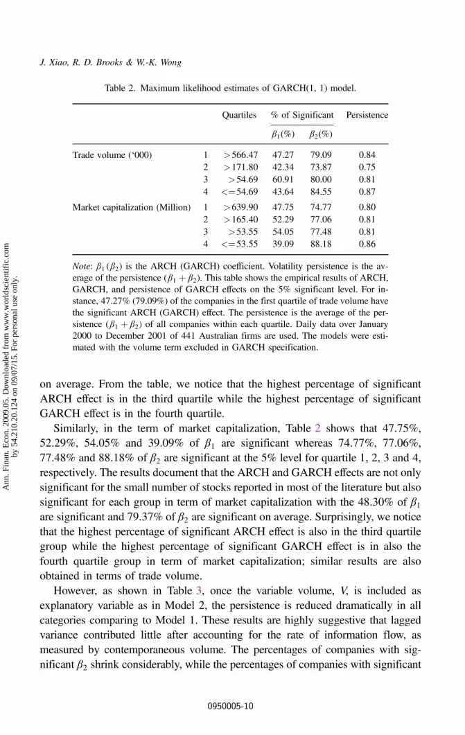
on average. From the table, we notice that the highest percentage of significantARCH effect is in the third quartile while the highest percentage of significantGARCH effect is in the fourth quartile.

Similarly, in the term of market capitalization, Table 2 shows that 47.75%,52.29%, 54.05% and 39.09% of β1 are significant whereas 74.77%, 77.06%,77.48% and 88.18% of β2 are significant at the 5% level for quartile 1, 2, 3 and 4,respectively. The results document that the ARCH and GARCH effects are not onlysignificant for the small number of stocks reported in most of the literature but alsosignificant for each group in term of market capitalization with the 48.30% of β1are significant and 79.37% of β2 are significant on average. Surprisingly, we noticethat the highest percentage of significant ARCH effect is also in the third quartilegroup while the highest percentage of significant GARCH effect is in also thefourth quartile group in term of market capitalization; similar results are alsoobtained in terms of trade volume.

However, as shown in Table 3, once the variable volume, V, is included asexplanatory variable as in Model 2, the persistence is reduced dramatically in allcategories comparing to Model 1. These results are highly suggestive that laggedvariance contributed little after accounting for the rate of information flow, asmeasured by contemporaneous volume. The percentages of companies with sig-nificant β2 shrink considerably, while the percentages of companies with significant

Table 2. Maximum likelihood estimates of GARCH(1, 1) model.

Quartiles % of Significant Persistence

β1(%) β2(%)

Trade volume (‘000) 1 >566:47 47.27 79.09 0.842 >171:80 42.34 73.87 0.753 >54:69 60.91 80.00 0.814 <¼54:69 43.64 84.55 0.87

Market capitalization (Million) 1 >639:90 47.75 74.77 0.802 >165:40 52.29 77.06 0.813 >53:55 54.05 77.48 0.814 <¼53:55 39.09 88.18 0.86

Note: β1 (β2) is the ARCH (GARCH) coefficient. Volatility persistence is the av-erage of the persistence (β1 þ β2). This table shows the empirical results of ARCH,GARCH, and persistence of GARCH effects on the 5% significant level. For in-stance, 47.27% (79.09%) of the companies in the first quartile of trade volume havethe significant ARCH (GARCH) effect. The persistence is the average of the per-sistence (β1 þ β2) of all companies within each quartile. Daily data over January2000 to December 2001 of 441 Australian firms are used. The models were esti-mated with the volume term excluded in GARCH specification.

J. Xiao, R. D. Brooks & W.-K. Wong

0950005-10

Ann

. Fin

an. E

con.

200

9.05

. Dow

nloa

ded

from

ww

w.w

orld

scie

ntif

ic.c

omby

54.

210.

20.1

24 o

n 09

/07/

15. F

or p

erso

nal u

se o

nly.

estimates of the volume coefficient are notably larger. So, our finding is that dailytrading volume has significant explanatory power, which shows similar behaviourin the Australian stock market to that observed in the US stock market (Lamoureuxand Lastrapes, 1990a) and in the Chinese stock market (Wong and Bian, 2005).

Before we analyze the results with volume variable in the model for all thestocks as shown Table 3, we first analyze the situation for the top 20 most activestocks in Australian market. The results are shown in Tables 4 and 5. We firstdiscuss the results shown in Table 4 for the model without volume variable. Thetable reveals that 45% of the ARCH effect (β1) are significant whereas most (90%)of the GARCH effect (β2) are significant. However, to consist with the findings inmost paper, with the volume variable is included, most of β1 and β2 becomeinsignificant — only 10% of β1 are significant and 15% of β2 are significant while70% of β3 are significant.

Now we come back to analyze the results with the volume variable in the modelfor all the stocks as shown in Table 3. Comparing with the results in Table 2, theresults in Table 3 do indicate that both ARCH and GARCH effects have beeneliminated significantly when the volume variable is included but the effect is notso much as those displayed in Table 5 for the top 20 most active stocks. Ourfindings infer that the volume variable does eliminate significantly the ARCH and

Table 3. Maximum likelihood estimates of GARCH(1, 1) model with volume.

Quartiles % of Significant Persistence

i1(%) β2(%) β3(%)

Trade volume (‘000) 1 >566:47 29.63 26.85 61.11 0.342 >171:80 31.78 34.58 45.79 0.423 >54:69 51.38 47.71 39.45 0.534 <¼54:69 33.33 60.19 28.70 0.61

Market capitalization (Million) 1 >639:90 25.93 28.70 61.11 0.352 >165:40 46.23 41.51 40.57 0.503 >53:55 40.91 52.73 36.36 0.554 <¼53:55 33.33 45.37 42.59 0.47

Note: β1(β2) is the ARCH (GARCH) coefficient. β3 is the coefficient capturing thevolume effect on conditional volatility. Volatility persistence is the average of the persis-tence (β1 þ β2) of all companies. This table shows the the empirical results of ARCH,GARCH, volume, and persistence of GARCH effects on the 5% significant level. Forinstance, For instance, 26.63% (26.85%) of the companies in the first quartile of tradevolume have the significant ARCH (GARCH) effect, while 61.11% of the companies havethe significant volume effect. The persistence is the average of the persistence (β1 þ β2) ofall companies within each quartile. Daily data over January 2000 to December 2001 of 441Australian firms are used. The models were estimated with the volume term included inGARCH specification.

GARCH and Volume Effects in the Australian Stock Markets

0950005-11

Ann

. Fin

an. E

con.

200

9.05

. Dow

nloa

ded

from

ww

w.w

orld

scie

ntif

ic.c

omby

54.

210.

20.1

24 o

n 09

/07/

15. F

or p

erso

nal u

se o

nly.

GARCH effects for many stocks in the entire Australian stock market but theelimination is not as much as the effect on the top 20 most active stocks.

We then turn to study the effect for different quartiles. Table 3 shows that thevolume variable eliminates both of the ARCH and GARCH effects for most for thequartile with the largest volume and with the largest market capitalization. Inaddition, comparing the results across the different quartiles, we find that thepercentage of companies having significant estimates of volume is considerablyhigher for the high trading volume stocks (quartile 1) than the thinly traded stocks.Meanwhile, the large companies are more likely have significant estimates of

Table 4. Maximum likelihood estimates of GARCH(1, 1) model for top 20active stocks.

# Co. Daily Average TradeVolume (‘000)

β1 β2 Persistence

1 TLSS 20088.85 0.2751* 0.5284** 0.80352 BHPY 12315.19 0.1740** 0.6217** 0.79573 CSRA 10803.15 0.0412 0.7721** 0.81334 WMCX 8056.94 0.1261** 0.8554** 0.98165 HILX 6789.94 0.0350 0.9350** 0.97006 PENC 6564.99 0.1631** 0.5644** 0.72757 MACM 6333.72 0.0740* 0.9003** 0.97438 FOST 6217.30 0.0541 0.9276** 0.98179 BHPS 5329.81 0.1245 0.0416 0.166110 PSAX 5169.16 0.1015** 0.7412** 0.842711 WEBA 4725.68 0.0909* 0.8653** 0.956212 OMIX 4385.73 0.0419 0.7291** 0.771013 ANBG 4314.41 0.0993** 0.7874** 0.886614 WTFD 4203.41 0.0280* 0.9629** 0.990915 MOSX 4165.68 0.0861 0.8812** 0.967216 WFAX 4159.07 0.0730 0.9113** 0.984317 QBEI 4154.90 0.1678 0.0000 0.167818 HDRU 3941.51 0.2053 0.7269** 0.932219 HLDX 3870.61 0.0240 0.9480** 0.971920 BRAI 3849.12 0.4588 0.5079** 0.9667

45% 90%

Note: β1(β2) is the ARCH (GARCH) coefficient. β3 is the coefficient cap-turing the volume effect on conditional volatility. Volatility persistence is theaverage of the persistence (β1 þ β2) of all companies.** means p-value less than 1%; * means p-value less than 5%. The entries inthe last row show the percentages of significant β’s. This table shows theempirical results of ARCH, GARCH, and persistence of GARCH effects inthe GARCH(1,1) model with volume term excluded. Most of the β2’s aresignificantly different to zero. The persistence of most stocks is near 1.

J. Xiao, R. D. Brooks & W.-K. Wong

0950005-12

Ann

. Fin

an. E

con.

200

9.05

. Dow

nloa

ded

from

ww

w.w

orld

scie

ntif

ic.c

omby

54.

210.

20.1

24 o

n 09

/07/

15. F

or p

erso

nal u

se o

nly.

volume than the small ones. Hence, we conclude that the actively traded stockswhich may have a larger number of information arrivals per day, leads to a largerimpact on the variance of daily returns.

4. Conclusion

This paper analyses the volume–volatility relationship for individual stock datataking into account both firm size and trading volume. Our analysis producesseveral major findings. First, trading volume has significant explanatory power for

Table 5. Maximum likelihood estimates of GARCH (1, 1) model with volume for top 20active stocks.

# Co. Daily Average TradeVolume (‘000)

β1 β2 β3 Persistence

1 TLSS 20088.85 0.0000 0.0000 0.0132** 0.00002 BHPY 12315.19 0.2407* 0.0000 0.0233** 0.24073 CSRA 10803.15 0.0494 0.0981 0.0102* 0.14744 WMCX 8056.94 0.0000 0.0000 0.0484** 0.00005 HILX 6789.94 0.0000 0.0000 0.1339** 0.00006 PENC 6564.99 0.0000 0.0000 0.9273 0.00007 MACM 6333.72 0.0000 0.0000 0.0445** 0.00008 FOST 6217.30 0.1777 0.0004 0.0178** 0.17829 BHPS 5329.81 0.0227 0.0000 0.0249* 0.022710 PSAX 5169.16 0.0000 0.0000 0.2448** 0.000011 WEBA 4725.68 0.0000 0.0000 0.0383** 0.000012 OMIX 4385.73 0.0000 0.0000 0.1071** 0.000013 ANBG 4314.41 0.0000 0.0000 0.0436** 0.000014 WTFD 4203.41 0.1542** 0.4665** 0.0064 0.620715 MOSX 4165.68 0.0959 0.8823** 0.0147 0.978216 WFAX 4159.07 0.0725 0.8875** -0.0004 0.959917 QBEI 4154.90 0.0353 0.0000 0.1106 0.035318 HDRU 3941.51 0.0000 0.1316 0.0477 0.131619 HLDX 3870.61 0.0000 0.0000 0.2413** 0.000020 BRAI 3849.12 0.0000 0.0000 0.0736** 0.0000

10% 15% 70%

Note: β1(β2) is the ARCH (GARCH) coefficient. β3 is the coefficient capturing the volumeeffect on conditional volatility. Volatility persistence is the average of the persistence(β1 þ β2) of all companies.** means p-value less than 1%; * means p-value less than 5%. The entries in the last rowshow the percentages of significant β’s. This table shows the empirical results of GARCH(1,1) model with volume term included. Most of the β3’s are significantly different to zero.Namely, GARCH effect mostly be token out after introducing the volume term. Thepersistence is reduced dramatically.

GARCH and Volume Effects in the Australian Stock Markets

0950005-13

Ann

. Fin

an. E

con.

200

9.05

. Dow

nloa

ded

from

ww

w.w

orld

scie

ntif

ic.c

omby

54.

210.

20.1

24 o

n 09

/07/

15. F

or p

erso

nal u

se o

nly.

the variance of daily return. This fits the old Wall Street adage that “it takes volumeto move price”. A herd effort could then be created and increasing traders will joinin, which will create further volatility. So, it is not surprising that volume can be agood proxy of information flows and replace the GARCH effect in the model. Thisimplies that the earlier findings in the literature were not a statistical fluke and that,unlike most anomalies, the volume effect on volatility is not likely to be eliminatedafter its discovery.

Second, based on the first conclusion, a stronger finding on the volume–vola-tility relationship is presented for the actively traded stocks, where trading volumehas a greater contribution in reducing GARCH effects. The top 20 active stocksshow the even stronger relationship between volume and volatility. However, oneof the explanations of thinly traded stocks with less significant volume–volatilityrelationship can be found in Brooks et al. (2005). For thin trading stocks, thefrequent occurrences of zero returns weaken the parameter estimation. The se-lectivity corrected market model in Brooks et al. (2005) suggests that, even for thethinly traded stocks, volume and volatility terms feature in the variance component.

Thirdly, our results indicate that low trading volume and small firm size lead toa higher persistence of GARCH effects in the estimated models with the volumeterm excluded in the variance equation. For the model with the volume termincluded, we find low trading volume stocks still have the highest persistence ofGARCH effects, but this not necessarily true for small firms.

Fourth, unlike the elimination effect for the top most active stocks, in general,the elimination of both ARCH and GARCH effects by introducing the volumevariable on all other stocks on average is not as much as that for the top most activestocks. In addition, the elimination of both ARCH and GARCH effects by intro-ducing the volume variable is higher for stocks in the largest volume and/or thelargest market capitialization quartile group.

Most anomalies, for example, the January effect, will diminish and eventuallydisappear after their discovery as more and more investors exploit the effect. Forexample, after discovering the January effect, investors who expect a stock’s priceto appreciate in January will then purchase the stock before January and sell it atthe end of January to make a profit. This will drive up stock prices before Januaryand push down prices at the end of January and will result in the diminishing oreven the disappearance of the January effect. For the volume–volatility relation-ship, it is a different story. Volatility will create further volatility, and more andmore investors will trade to take advantage of the active market. Hence, volumeand turnover will increase and this phenomenon will last for quite a while. Basedon the findings in this paper, we hypothesize that, unlike other anomalies, both theGARCH effect and the volume–volatility relationship will not be able to beexploited by investors and will persist in the market. Our findings imply that the

J. Xiao, R. D. Brooks & W.-K. Wong

0950005-14

Ann

. Fin

an. E

con.

200

9.05

. Dow

nloa

ded

from

ww

w.w

orld

scie

ntif

ic.c

omby

54.

210.

20.1

24 o

n 09

/07/

15. F

or p

erso

nal u

se o

nly.

earlier findings in the literature were not a statistical fluke and that, unlike mostanomalies, the volume effect on volatility is not likely to be eliminated after itsdiscovery. In addition, the existence of both the GARCH effect and the volume–volatility relationship leads us to reject the pure random walk hypothesis for stockreturns.

Understanding the relationship between volume and volatility will be useful ininvestment decision making. Recently, Lam et al. (2010) have developed aBayesian behavior finance model to explain excess volatility. This model couldbe useful in explaining the volume–volatility relationship. Understanding thebehaviors of different types of investors, including risk averters and risk seekers(Wong and Li, 1999; Li and Wong, 1999; Wong, 2007; Sriboonchita et al., 2009;Egozcue and Wong, 2010; Ma and Wong, 2010), investors with S-shaped andreversed S-shaped utility functions (Wong and Chan, 2008; Broll et al., 2010) intheir investment decision-making could also be used to explain the volume–vol-atility relationship. In addition, the information of the companies (Thompson andWong, 1991, 1996; Wong and Chan, 2004), the economic and financial environ-ment (Wong and Li, 1999; Fong et al., 2005, 2008; Broll et al., 2006; Gasbarroet al., 2007; Wong and Ma, 2008; Wong et al., 2008; Lean et al., 2007, 2010)can also be used to make better investment decisions. Another extension thatwould improve investment decision making is to include technical analysis (Wonget al., 2001, 2003) that incorporates the volume volatility relationship. One couldalso apply advanced econometrics (for example Wong and Miller, 1990; Matsu-mura et al., 1990; Tiku et al., 2000; Wong and Bian, 2005; Leung andWong, 2008; Bai et al., 2009a,b, 2010) to make better investment decisions.

Statement of Relationship to Practice

Our findings on the ARCH, GARCH, volume, and volatility effects in the Aus-tralian stock market are useful for practitioners in their investment decision mak-ing. For example, we find that that all the ARCH, GARCH, volume, and volatilityeffects are the largest for the groups with largest firm sizes and/or largest tradingvolumes. This information is useful for practitioners in their investment decisionmaking.

References

Admati, AR and P Pfleiderer (1988). A theory of intraday patterns: Volume and pricevariability. Review of Financial Studies, 1, 3–40.

Andersen, T (1996). Return volatility and trading volume: An information flow interpre-tation. Journal of Finance, 51, 169–204.

GARCH and Volume Effects in the Australian Stock Markets

0950005-15

Ann

. Fin

an. E

con.

200

9.05

. Dow

nloa

ded

from

ww

w.w

orld

scie

ntif

ic.c

omby

54.

210.

20.1

24 o

n 09

/07/

15. F

or p

erso

nal u

se o

nly.

Andrew, WL and W Jiang (2000). Trading volume, definition, data analysis and impli-cations of portfolio theory. Review of Financial Studies, 13, 257–300.

Aragó, V and L Nieto (2005). Heteroskedasticity in the returns of the main world stockexchange indices: Volume versus GARCH effects. Journal of International FinancialMarkets, Institutions and Money, 15, 271–284.

Bai, ZD, HX Liu and WKWong (2009a). Enhancement of the applicability of Markowitz’sportfolio optimization by utilizing random matrix theory. Mathematical Finance, 19(4),639–667.

Bai, ZD, HX Liu and WK Wong (2009b). On the Markowitz mean-variance analysis ofself–financing portfolios. Risk and Decision Analysis, 1(1), 35–42.

Bai, ZD, WK Wong and B Zhang (2010). Multivariate linear and nonlinear causality tests.Mathematics and Computers in Simulation, Forthcoming.

Baillie, RT and T Bollerslev (1989). The message in daily exchange rates: A conditionalvariance tale. Journal of Business and Economic Statistics, 7, 297–305.

Bollerslev, T (1986). Generalised conditional autoregressive heteroskedasticity. Journal ofEconometrics, 31, 307–327.

Bollerslev, T (1987). A conditional heteroskedasticity time series model for speculativeprices and rates of return. Review of Economics and Statistics, 6, 542–547.

Bollerslev, T, RY Chou and KF Kroner (1992). ARCH modeling in finance. Journal ofEconometrics, 52, 5–59.

Bollerslev, T, RF Engle and DB Nelson (1994). ARCH Model. In Engle, RF and DCMcfadden (Eds.), Handbook of Econometrics IV, pp. 2959–3038. Amsterdam: ElsevierScience.

Broll, U, JE Wahl and WKWong (2006). Elasticity of risk aversion and international trade.Economics Letters, 92(1), 126–130.

Broll, U, M Egozcue, WKWong and R Zitikis (2010). Prospect theory, indifference curves,and hedging risks. Applied Mathematics Research Express, Forthcoming.

Brooks, R, R Faff and M Mckenzie (2000a). Bivariate GARCH estimation of beta risk inthe Australian banking industry. Accountability Performance, 3, 81–102.

Brooks, R, R Faff, Y Ho and M Mckenzie (2000b). US banking sector risk in an era ofregulatory change: A bivariate GARCH approach. Review of Quantitative FinanceAccounting, 14, 17–43.

Brooks, R, R Faff and T Fry (2001). GARCH modelling of individual stock data: Theimpact of censoring, firm size and trading volume. Journal of International FinancialMarkets, Institutions and Money, 11, 215–222.

Brooks, R, R Faff, T Fry and Newton, E (2005). The selectivity corrected market modeland heteroscedasticity in stock returns: Volume versus GARCH revisited. AccountingResearch Journal, 17, 192–201.

Campbell, J, S Grossman and J Wang, J (1993). Trading volume and serial correlation inStock Returns, Quarterly Journal of Economics, 108, 905–939.

Clark, PK (1973). A subordinate stochastic process model with finite variance for spec-ulative prices. Econometrica, 41(1), 135–155.

Conrad, J, A Hammeed and C Niden (1994). Volume and autocovariances in short-horizonindividual security returns. Journal of Finance, 49, 1305–1329.

Copeland, TE (1976). A model of asset trading under the assumption of sequential in-formation arrival. Journal of Finance, 31, 1149–1168.

J. Xiao, R. D. Brooks & W.-K. Wong

0950005-16

Ann

. Fin

an. E

con.

200

9.05

. Dow

nloa

ded

from

ww

w.w

orld

scie

ntif

ic.c

omby

54.

210.

20.1

24 o

n 09

/07/

15. F

or p

erso

nal u

se o

nly.

Daigler, RT and MK Wiley (1999). The impact of trader type on the futures volatility–volume relation. Journal of Finance, 6, 2297–2316.

Diebold, FX (1986). Comment on modeling the persistence of conditional variance.Econometric Reviews, 5, 51–56.

Ding, Z and CWJ Granger (1996). Modeling volatility persistence of speculative returns: Anew approach. Journal of Econometrics, 73, 185–215.

Egozcue, M and WK Wong (2010). Gains from diversification on convex combinations: Amajorization and stochastic dominance approach. European Journal of OperationalResearch, Forthcoming.

Engle, R (1982). Autoregressive conditional heteroskedasticity with estimates of the var-iance of United Kingdom inflation. Econometrica, 50, 987–1007.

Engle, R and C Mustafa (1992). Implied ARCH models from option price. Journal ofEconometrics, 52, 289–311.

Engle, RF and KF Kroner (1995). Multivariate simultaneous generalized ARCH. Econo-metric Theory, 11, 122–150.

Epps, T and M Epps (1976). The stochastic dependence of security price changes andtransaction volumes: Implications for the mixture of distributions hypothesis. Econo-metrica, 44, 305–321.

Fong, WM and WK Wong (2006). The modified mixture of distributions model: A revisit.Annals of Finance, 2(4), 167–178.

Fong, WM, HH Lean and WK Wong (2008). Stochastic dominance and behavior towardsrisk: The market for internet stocks. Journal of Economic Behavior and Organization,68(1), 194–20.

Fong, WM, WK Wong and HH Lean (2005). Stochastic dominance and the rationality ofthe momentum effect across markets. Journal of Financial Markets, 8, 89–109.

Gallant, R, PE Rossi and G Tauchen (1992). Stock prices and volumes. Review of Fi-nancial Studies, 5, 199–244.

Gasbarro, D, WK Wong and JK Zumwalt (2007). Stochastic dominance analysis of Ishares. European Journal of Finance, 13, 89–101.

Gonzales-Rivera, G (1996). Time varying risk: The case of the American computer in-dustry. Journal of Empirical Finance, 2, 333–342.

Harris, L (1986). Cross-security tests of the mixture of distributions hypothesis. Journal ofFinancial and Quantitative Analysis, 21, 39–46.

Harris, L (1987). Transaction data tests of the mixture of distributions hypothesis. Journalof Financial Quantitative Analysis, 2, 127–141.

Harris, M and A Raviv (1993). Differences of opinion make a horse race. Review ofFinancial Studies, 6, 473–506.

Hiemstra, C and J Jones (1994). Testing for linear and nonlinear granger causality in thestock price-volume relation. Journal of Finance, 49, 1639–1664.

Hsieh, D (1988). The statistical properties of daily foreign exchange rates: 1974–1984.Journal of International Economics, 24, 129–145.

Hsieh, D (1989). Modelling heteroskedasticity in daily foreign-exchange rates. Journal ofBusiness Economic Statistics, 7, 307–317.

Jennings, R, L Starks and J Fellingham (1981). An equilibrium model of asset trading withsequential information arrival. Journal of Finance, 36, 143–161.

GARCH and Volume Effects in the Australian Stock Markets

0950005-17

Ann

. Fin

an. E

con.

200

9.05

. Dow

nloa

ded

from

ww

w.w

orld

scie

ntif

ic.c

omby

54.

210.

20.1

24 o

n 09

/07/

15. F

or p

erso

nal u

se o

nly.

Jones, CM, G Kaul and ML Lipson (1994). Transactions, volume and volatility. Review ofFinancial Studies, 7(4), 631–651.

Kim, D and S Kon (1994). Alternative models for the conditional heteroscedasticity ofstock returns. Journal of Business, 67, 563–588.

Kyle, AS (1985). Continuous auctions and insider trading. Econometrica, 53, 1315–1335.Lakonishok, J and S Smidt (1986). Volume for winners and losers: Taxation and other

motives for stock trading. Journal of Finance, 41, 951–974.Lam, K, T Liu and WK Wong (2010). A pseudo-Bayesian model in financial decision

making with implications to market volatility, under- and overreaction. EuropeanJournal of Operational Research, Forthcoming.

Lamoureux, CG and WD Lastrapes (1990a). Heteroskedasaticity in stock returns data:Volume versus GARCH effects. Journal of Finance, 45(1), 221–229.

Lamoureux, CG and WD Lastrapes (1990b). Persistence in variance, structural change andthe GARCH model. Journal of Business Economic Statistic, 8, 225–234.

Lange, S (1999). Modeling asset market volatility in a small market: Accounting from non-synchronous trading effects. Journal of Finance, 45, 221–229.

Lean, HH, M Mcaleer and WK Wong (2010). Market efficiency of oil spot andfutures: A mean-variance and stochastic dominance approach. Energy Economics,Forthcoming.

Lean, HH, R Smyth and WK Wong (2007). Revisiting calendar anomalies in Asian stockmarkets using a stochastic dominance approach. Journal of Multinational FinancialManagement, 17(2), 125–141.

Leung, PL and WK Wong (2008). On testing the equality of the multiple sharpe ratios,with application on the evaluation of Ishares. Journal of Risk, 10(3), 1–16.

Li, CK and WK Wong (1999). Extension of stochastic dominance theory to randomvariables. RAIRO — Recherche Op�ERationnelle, 33(4), 509–524.

Lo, WA and J Wang (2000). Trading volume: Definitions, data analysis, and implicationsof portfolio theory. Review of Financial Studies, 13, 257–300.

Ma, C and WKWong (2010). Stochastic dominance and risk measure: A decision-theoreticfoundation for Var and C-Var. European Journal of Operational Research, Forthcom-ing.

Matsumura, EM, KW Tsui and WK Wong (1990). An extended multinomial-Dirichletmodel for error nounds for dollar-unit sampling. Contemporary Accounting Research,6(2-I), 485–500.

Mcclain, KT, HB Humprehys and A Boscan (1996). Measuring risk in the mining sectorwith ARCH models with important observations on sample size. Journal of EmpiricalFinance, 3. 369–391. Mccurdy, T and I Morgan (1987). Tests of Martingale hypothesisfor foreign currency futures with time varying volatility. International Journal ofForecasting, 3, 131–148.

Miyakoshi, T (2002). ARCH versus information-based variances: Evidence from theTokyo stock market. Japan and the World Economy, 2, 215–231.

Morse, D (1980). Asymmetric information in securities markets and trading volume.Journal of Financial and Quantitative Analysis, 15, 1129–1148.

Ragunathan, V and A Peker (1997). Price variability, trading volume, and marketepth: Evidence from the Australian futures market. Applied Financial Economics, 5,447–454.

J. Xiao, R. D. Brooks & W.-K. Wong

0950005-18

Ann

. Fin

an. E

con.

200

9.05

. Dow

nloa

ded

from

ww

w.w

orld

scie

ntif

ic.c

omby

54.

210.

20.1

24 o

n 09

/07/

15. F

or p

erso

nal u

se o

nly.

Royston, P (1982). An extension of Shapiro and Wilk’s W test for normality to largesamples. Applied Statistics, 31, 115–124.

Shalen, CT (1993). Volume, volatility and the dispersion of beliefs. Review of FinancialStudies, 6, 405–434.

Sharma, LJ, M Mougoue and R Kamath (1996). Heteroscedasticity in stock market in-dicator return data: Volume versus GARCH effects. Applied Financial Economics, 6,337–342.

Smidt, S (1990). Long-run trends in equity turnover. Journal of Portfolio Management, 17,66–73.

Smirlock, M and L Starks (1985). A further examination of stock price changes andtransaction volume. Journal of Financial Research, 8, 217–225.

Song, F (1994). A two-factor ARCH model for deposit-institution stock returns. Journal ofMoney Credit Banking, 26, 323–340.

Sriboonchita, S, WK Wong, S Dhompongsa and HT Nguyen (2009). Stochastic Domi-nance and Applications to Finance, Risk and Economics. Chapman and Hall/CRC,Taylor and Francis Group: Boca Raton, Florida, USA.

Stock, JH (1987). Measuring business cycle time. Journal of Political Economy, 95, 1240–1261.

Tauchen, GE and M Pitts (1983). The price variability–volume relationship on speculativemarkets. Econometrica, 51(2), 485–505.

Thompson, HE and WK Wong (1991). On the unavoidability of ‘unscientific’ judgment inestimating the cost of capital. Managerial and Decision Economics, 12, 27–42.

Thompson, HE and WK Wong (1996). Revisiting ‘dividend yield plus growth’ anditsaApplicability. Engineering Economist, 41(2), 123–147.

Tiku, ML, WK Wong, DC Vaughan and G Bian (2000). Time series models with non-normal innovations: Symmetric location-scale distributions. Journal of Time SeriesAnalysis, 21(5), 571–596.

Varian, H (1985). Divergence of opinion in complete markets: A note. Journal of Finance,40, 309–317.

Wong, WK (2007). Stochastic dominance and mean-variance measures of profit and lossfor business planning and investment. European Journal of Operational Research, 182,829–843.

Wong, WK and C Ma (2008). Preferences over location-scale family. Economic Theory,37(1), 119–146.

Wong, WK and CK Li (1999). A note on convex stochastic dominance theory. EconomicsLetters, 62, 293–300.

Wong, WK and G Bian (2005). Estimating parameters in autoregressive models withasymmetric innovations. Statistics and Probability Letters, 71, 61–70.

Wong, WK and R Chan (2004). The estimation of the cost of capital and its reliability.Quantitative Finance, 4(3), 365–372.

Wong, WK and R Chan (2008). Markowitz and prospect stochastic dominances. Annals ofFinance, 4(1), 105–129.

Wong, WK and RB Miller (1990). Analysis of ARIMA-noise models with repeated timeseries. Journal of Business and Economic Statistics, 8(2), 243–250.

Wong, WK, BK Chew and D Sikorski (2001). Can P/E ratio and bond yield be used to beatstock markets. Multinational Finance Journal, 5(1), 59–86.

GARCH and Volume Effects in the Australian Stock Markets

0950005-19

Ann

. Fin

an. E

con.

200

9.05

. Dow

nloa

ded

from

ww

w.w

orld

scie

ntif

ic.c

omby

54.

210.

20.1

24 o

n 09

/07/

15. F

or p

erso

nal u

se o

nly.

Wong, WK, M Manzur and BK Chew (2003). How rewarding is technical analysis?Evidence from Singapore stock market. Applied Financial Economics, 13(7), 543–551.

Wong, WK, PL Leung and J Xu (2005). The GARCH effects on the volume of China stockmarkets. International Journal of Finance, 17(1), 3290–3329.

Wong, WK, KF Phoon and HH Lean (2008). Stochastic dominance analysis of Asianhedge funds. Pacific-Basin Finance Journal, 16(3), 204–223.

J. Xiao, R. D. Brooks & W.-K. Wong

0950005-20

Ann

. Fin

an. E

con.

200

9.05

. Dow

nloa

ded

from

ww

w.w

orld

scie

ntif

ic.c

omby

54.

210.

20.1

24 o

n 09

/07/

15. F

or p

erso

nal u

se o

nly.