exercises 7.1
TRANSCRIPT
7.1 DEFINITION OF THE LAPLACE TRANSFORM ● 261
EXERCISES 7.1 Answers to selected odd-numbered problems begin on page ANS-10.
In Problems 1–18 use Definition 7.1.1 to find �{ f (t)}.
1.
2.
3.
4.
5.
6.
7.
f (t) � �0,
cos t,
0 � t � �>2t � �>2
f (t) � �sin t,
0,
0 � t � �
t � �
f (t) � �2t � 1,
0,
0 � t � 1
t � 1
f (t) � � t,
1,
0 � t � 1
t � 1
f (t) � �4,
0,
0 � t � 2
t � 2
f (t) � ��1,
1,
0 � t � 1
t � 1
9.
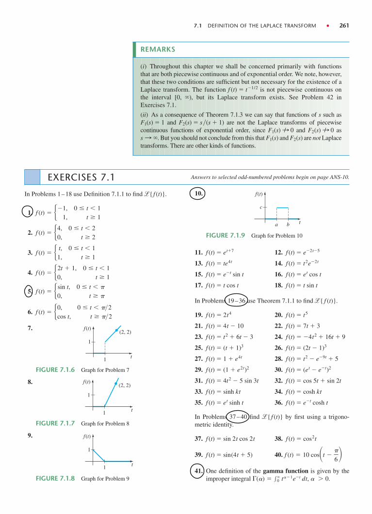
FIGURE 7.1.7 Graph for Problem 8
FIGURE 7.1.8 Graph for Problem 9
FIGURE 7.1.9 Graph for Problem 10
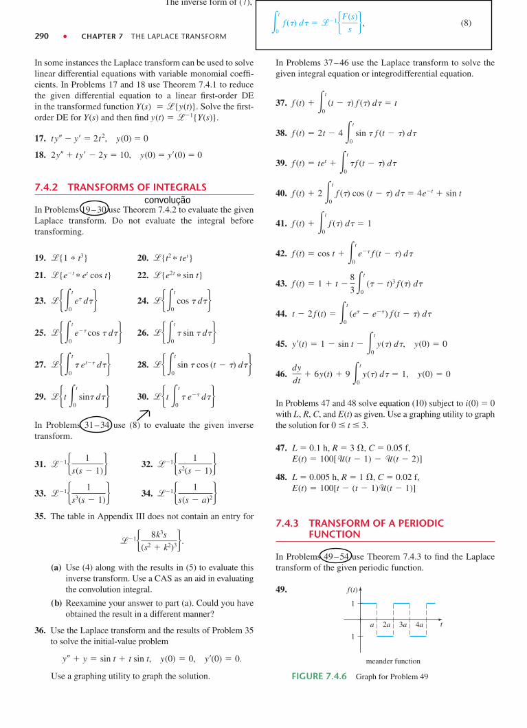
t
f(t)(2, 2)
1
1
FIGURE 7.1.6 Graph for Problem 7
t
f(t)(2, 2)
1
1
t
f(t)
1
1
f(t)
a
c
b t
8.
10.
11. f (t) � et�7 12. f (t) � e�2t�5
13. f (t) � te4t 14. f (t) � t2e�2t
15. f (t) � e�t sin t 16. f (t) � et cos t
17. f (t) � t cos t 18. f (t) � t sin t
In Problems 19–36 use Theorem 7.1.1 to find �{ f (t)}.
19. f (t) � 2t4 20. f (t) � t5
21. f (t) � 4t � 10 22. f (t) � 7t � 3
23. f (t) � t2 � 6t � 3 24. f (t) � �4t2 � 16t � 9
25. f (t) � (t � 1)3 26. f (t) � (2t � 1)3
27. f (t) � 1 � e4t 28. f (t) � t2 � e�9t � 5
29. f (t) � (1 � e2t)2 30. f (t) � (et � e�t)2
31. f (t) � 4t2 � 5 sin 3t 32. f (t) � cos 5t � sin 2t
33. f (t) � sinh kt 34. f (t) � cosh kt
35. f (t) � et sinh t 36. f (t) � e�t cosh t
In Problems 37–40 find �{ f (t)} by first using a trigono-metric identity.
37. f (t) � sin 2t cos 2t 38. f (t) � cos2t
39. f (t) � sin(4t � 5) 40.
41. One definition of the gamma function is given by theimproper integral �(�) � �
0 t��1e�t dt, � � 0.
f (t) � 10 cos�t ��
6�
REMARKS
(i) Throughout this chapter we shall be concerned primarily with functionsthat are both piecewise continuous and of exponential order. We note, however,that these two conditions are sufficient but not necessary for the existence of aLaplace transform. The function f (t) � t�1/2 is not piecewise continuous onthe interval [0, ), but its Laplace transform exists. See Problem 42 inExercises 7.1.
(ii) As a consequence of Theorem 7.1.3 we can say that functions of s such asF1(s) � 1 and F2(s) � s�(s � 1) are not the Laplace transforms of piecewise continuous functions of exponential order, since F1(s) 0 and F2(s) 0 as
. But you should not conclude from this that F1(s) and F2(s) are not Laplacetransforms. There are other kinds of functions.s :
:/:/
262 ● CHAPTER 7 THE LAPLACE TRANSFORM
(a) Show that �(a � 1) � a�(a).
(b) Show that .
42. Use the fact that and Problem 41 to find theLaplace transform of
(a) f (t) � t�1/2 (b) f (t) � t1/2 (c) f (t) � t3/2.
Discussion Problems
43. Make up a function F(t) that is of exponential order butwhere f (t) � F�(t) is not of exponential order. Make upa function f that is not of exponential order but whoseLaplace transform exists.
44. Suppose that for s c1 and thatfor s c2. When does
45. Figure 7.1.4 suggests, but does not prove, that the func-tion is not of exponential order. How doesf (t) � et 2
�{f1(t) � f2(t)} � F1(s) � F2(s)?
��{ f2(t)} � F2(s)��{ f1(t)} � F1(s)
�(12) � 1�
�{t�} ��(� � 1)
s��1 , � � �1
the observation that for and tsufficiently large, show that for any c?
46. Use part (c) of Theorem 7.1.1 to show that
�{e(a�ib)t} � , where a and b are real
and i2 � �1. Show how Euler’s formula (page 134) canthen be used to deduce the results
.
47. Under what conditions is a linear functionf (x) � mx � b, m � 0, a linear transform?
48. The proof of part (b) of Theorem 7.1.1 requiresthe use of mathematical induction. Show that if�{tn�1} � (n � 1)!�sn is assumed to be true, then�{tn} � n!�sn�1 follows.
�{eat sin bt} �b
(s � a)2 � b2
�{eat cos bt} �s � a
(s � a)2 � b2
s � a � ib
(s � a)2 � b2
et 2� Mect
M � 0t2 � ln M � ct,
INVERSE TRANSFORMS AND TRANSFORMS
OF DERIVATIVES
REVIEW MATERIAL● Partial fraction decomposition● See the Student Resource and Solutions Manual
INTRODUCTION In this section we take a few small steps into an investigation of howthe Laplace transform can be used to solve certain types of equations for an unknown function.We begin the discussion with the concept of the inverse Laplace transform or, more precisely,the inverse of a Laplace transform F(s). After some important preliminary background materialon the Laplace transform of derivatives f �(t), f ��(t), . . . , we then illustrate how both the Laplacetransform and the inverse Laplace transform come into play in solving some simple ordinarydifferential equations.
7.2
Transform Inverse Transform
e�3t � � �1� 1
s � 3��{e�3t} �1
s � 3
t � � �1�1
s2��{t} �1
s2
1 � � �1�1
s��{1} �1
s
7.2.1 INVERSE TRANSFORMS
THE INVERSE PROBLEM If F(s) represents the Laplace transform of a functionf (t), that is, , we then say f (t) is the inverse Laplace transform ofF(s) and write . For example, from Examples 1, 2, and 3 ofSection 7.1 we have, respectively,
f(t) � � �1{F(s)}�{ f(t)} � F(s)
7.2 INVERSE TRANSFORMS AND TRANSFORMS OF DERIVATIVES ● 269
The desired decomposition (15) is given in (4). This special technique fordetermining coefficients is naturally known as the cover-up method.
(iii) In this remark we continue our introduction to the terminology ofdynamical systems. Because of (9) and (10) the Laplace trans-form is well adapted to linear dynamical systems. The polynomial
in (11) is the total coefficient of Y(s) in(10) and is simply the left-hand side of the DE with the derivatives dky�dtk
replaced by powers sk, k � 0, 1, . . . , n. It is usual practice to call the recipro-cal of P(s)—namely, W(s) � 1�P(s)—the transfer function of the systemand write (11) as
. (16)
In this manner we have separated, in an additive sense, the effects on the responsethat are due to the initial conditions (that is, W(s)Q(s)) from those due to theinput function g (that is, W(s)G(s)). See (13) and (14). Hence the response y(t) ofthe system is a superposition of two responses:
.
If the input is g(t) � 0, then the solution of the problem is. This solution is called the zero-input response of the
system. On the other hand, the function is the output dueto the input g(t). Now if the initial state of the system is the zero state (all theinitial conditions are zero), then Q(s) � 0, and so the only solution of the initial-value problem is y1(t). The latter solution is called the zero-state response of thesystem. Both y0(t) and y1(t) are particular solutions: y0(t) is a solution of the IVPconsisting of the associated homogeneous equation with the given initial condi-tions, and y1(t) is a solution of the IVP consisting of the nonhomogeneous equa-tion with zero initial conditions. In Example 5 we see from (14) that the transferfunction is W(s) � 1�(s2 � 3s � 2), the zero-input response is
,
and the zero-state response is
.
Verify that the sum of y0(t) and y1(t) is the solution y(t) in Example 5 and thaty0(0) � 1, , whereas y1(0) � 0, .y�1(0) � 0y�0(0) � 5
y1(t) � � �1� 1
(s � 1)(s � 2)(s � 4)� � �1
5et �
1
6e2t �
1
30e�4t
y0(t) � � �1� s � 2
(s � 1)(s � 2)� � �3et � 4e2t
y1(t) � � �1{W(s)G(s)}y0(t) � � �1{W(s)Q(s)}
y(t) � � �1{W(s)Q(s)} � � �1{W(s)G(s)} � y0(t) � y1(t)
Y(s) � W(s)Q(s) � W(s)G(s)
P(s) � ansn � an�1sn�1 � � a0
EXERCISES 7.2 Answers to selected odd-numbered problems begin on page ANS-10.
7.2.1 INVERSE TRANSFORMS
In Problems 1–30 use appropriate algebra and Theorem 7.2.1to find the given inverse Laplace transform.
1. 2.
3. 4.
5. 6. � �1�(s � 2)2
s3 �� �1�(s � 1)3
s4 �
� �1��2
s�
1
s3�2
�� �1�1
s2 �48
s5�
� �1�1
s4�� �1�1
s3�
7. 8.
9. 10.
11. 12.
13. 14.
15. 16. � �1� s � 1
s2 � 2�� �1�2s � 6
s2 � 9�
� �1� 1
4s2 � 1�� �1� 4s
4s2 � 1�
� �1� 10s
s2 � 16�� �1� 5
s2 � 49�
� �1� 1
5s � 2�� �1� 1
4s � 1�
� �1�4
s�
6
s5 �1
s � 8�� �1�1
s2 �1
s�
1
s � 2�
270 ● CHAPTER 7 THE LAPLACE TRANSFORM
17. 18.
19. 20.
21.
22.
23.
24.
25. 26.
27. 28.
29. 30.
7.2.2 TRANSFORMS OF DERIVATIVES
In Problems 31–40 use the Laplace transform to solve thegiven initial-value problem.
31.
32.
33. y� � 6y � e4t, y(0) � 2
34. y� � y � 2 cos 5t, y(0) � 0
35. y � 5y� � 4y � 0, y(0) � 1, y�(0) � 0
36. y � 4y� � 6e3t � 3e�t, y(0) � 1, y�(0) � �1
37.
38. y � 9y � et, y(0) � 0, y�(0) � 0
y � y � 22 sin22t, y(0) � 10, y�(0) � 0
2dy
dt� y � 0, y (0) � �3
dy
dt� y � 1, y (0) � 0
� �1� 6s � 3
s4 � 5s2 � 4�� �1� 1
(s2 � 1)(s2 � 4)�
� �1� 1
s4 � 9�� �1� 2s � 4
(s2 � s)(s2 � 1)�
� �1� s
(s � 2)(s2 � 4)�� �1� 1
s3 � 5s�
� �1� s2 � 1
s(s � 1)(s � 1)(s � 2)�
� �1� s
(s � 2)(s � 3)(s � 6)�
� �1� s � 3
�s � 13 ��s � 13 ��
� �1� 0.9s
(s � 0.1)(s � 0.2)�
� �1� 1
s2 � s � 20�� �1� s
s2 � 2s � 3�
� �1� s � 1
s2 � 4s�� �1� 1
s2 � 3s� 39. 2y� � 3y � 3y� � 2y � e�t, y(0) � 0, y�(0) � 0,y(0) � 1
40. y� � 2y � y� � 2y � sin 3t, y(0) � 0, y�(0) � 0,y(0) � 1
The inverse forms of the results in Problem 46 inExercises 7.1 are
In Problems 41 and 42 use the Laplace transform and theseinverses to solve the given initial-value problem.
41. y� � y � e�3t cos 2t, y(0) � 0
42. y � 2y� � 5y � 0, y(0) � 1, y�(0) � 3
Discussion Problems
43. (a) With a slight change in notation the transform in (6)is the same as
With f (t) � teat, discuss how this result in conjunc-tion with (c) of Theorem 7.1.1 can be used to evalu-ate .
(b) Proceed as in part (a), but this time discuss how touse (7) with f (t) � t sin kt in conjunction with (d)and (e) of Theorem 7.1.1 to evaluate .
44. Make up two functions f1 and f2 that have the sameLaplace transform. Do not think profound thoughts.
45. Reread Remark (iii) on page 269. Find the zero-inputand the zero-state response for the IVP in Problem 36.
46. Suppose f (t) is a function for which f �(t) is piecewisecontinuous and of exponential order c. Use results inthis section and Section 7.1 to justify
,
where F(s) � �{ f (t)}. Verify this result withf (t) � cos kt.
f (0) � lims:
sF(s)
�{t sin kt}
�{teat}
�{ f �(t)} � s�{ f (t)} � f (0).
� �1� b
(s � a)2 � b2� � eat sin bt.
� �1� s � a
(s � a)2 � b2� � eat cos bt
OPERATIONAL PROPERTIES I
REVIEW MATERIAL● Keep practicing partial fraction decomposition● Completion of the square
INTRODUCTION It is not convenient to use Definition 7.1.1 each time we wish to find the Laplacetransform of a function f (t). For example, the integration by parts involved in evaluating, say,
is formidable, to say the least. In this section and the next we present several labor-saving operational properties of the Laplace transform that enable us to build up a more extensive list oftransforms (see the table in Appendix III) without having to resort to the basic definition and integration.
�{ett2 sin 3t}
7.3
278 ● CHAPTER 7 THE LAPLACE TRANSFORM
SOLUTION Recall that because the beam is embedded at both ends, the boundaryconditions are y(0) � 0, y�(0) � 0, y(L) � 0, y�(L) � 0. Now by (10) we can expressw(x) in terms of the unit step function:
Transforming (19) with respect to the variable x gives
or
If we let c1 � y(0) and c2 � y�(0), then
,
and consequently
Y(s) �c1
s3 �c2
s4 �2w0
EIL L>2s5 �
1
s6 �1
s6 e�Ls/2�
s4Y(s) � sy(0) � y�(0) �2w0
EIL L>2
s�
1
s2 �1
s2 e�Ls/2�.
EI�s4Y(s) � s3y(0) � s2y�(0) � sy(0) � y� (0)� �2w0
L L>2s
�1
s2 �1
s2 e�Ls/2�
�2w0
L L
2� x � �x �
L
2� ��x �L
2��.
w(x) � w0�1 �2
Lx� � w0�1 �
2
Lx� ��x �
L
2�
�c1
2x2 �
c2
6x3 �
w0
60 EIL 5L
2x4 � x5 � �x �
L
2�5
��x �L
2��.
y(x) �c1
2!� �1�2!
s3� �c2
3!� �1�3!
s4� �2w0
EIL L>24!
� �1�4!
s5� �1
5!� �1�5!
s6� �1
5!� �1�5!
s6 e�Ls/ 2��
Applying the conditions y(L) � 0 and y�(L) � 0 to the last result yields a system ofequations for c1 and c2:
Solving, we find c1 � 23w0L2�(960EI) and c2 � �9w0L�(40EI). Thus the deflec-tion is given by
y(x) �23w0L2
1920EIx2 �
3w0L
80EIx3 �
w0
60EIL 5L
2x4 � x5 � �x �
L
2�5
��x �L
2��.
c1 L � c2L2
2�
85w0L3
960EI� 0.
c1L2
2� c2
L3
6�
49w0L4
1920EI� 0
EXERCISES 7.3 Answers to selected odd-numbered problems begin on page ANS-11.
7.3.1 TRANSLATION ON THE s-AXIS
In Problems 1–20 find either F(s) or f (t), as indicated.
1. 2.
3. 4.
5. 6.
7. 8.
9.
10. ��e3t�9 � 4t � 10 sin t
2���{(1 � et � 3e�4t ) cos 5t}
�{e�2t cos 4t}�{et sin 3t}
�{e2t(t � 1)2}�{t(et � e2t)2}
�{t10e�7t}�{t3e�2t}
�{te�6t}�{te10t}
11. 12.
13. 14.
15. 16.
17. 18.
19. 20. � �1�(s � 1)2
(s � 2)4�� �1� 2s � 1
s2(s � 1)3�
� �1� 5s
(s � 2)2�� �1� s
(s � 1)2�
� �1� 2s � 5
s2 � 6s � 34�� �1� s
s2 � 4s � 5�
� �1� 1
s2 � 2s � 5�� �1� 1
s2 � 6s � 10�
� �1� 1
(s � 1)4�� �1� 1
(s � 2)3�
7.3 OPERATIONAL PROPERTIES I ● 279
In Problems 21–30 use the Laplace transform to solve thegiven initial-value problem.
21. y� � 4y � e�4t, y(0) � 2
22. y� � y � 1 � tet, y(0) � 0
23. y � 2y� � y � 0, y(0) � 1, y�(0) � 1
24. y � 4y� � 4y � t3e2t, y(0) � 0, y�(0) � 0
25. y � 6y� � 9y � t, y(0) � 0, y�(0) � 1
26. y � 4y� � 4y � t3, y(0) � 1, y�(0) � 0
27. y � 6y� � 13y � 0, y(0) � 0, y�(0) � �3
28. 2y � 20y� � 51y � 0, y(0) � 2, y�(0) � 0
29. y � y� � et cos t, y(0) � 0, y�(0) � 0
30. y � 2y� � 5y � 1 � t, y(0) � 0, y�(0) � 4
In Problems 31 and 32 use the Laplace transform andthe procedure outlined in Example 9 to solve the givenboundary-value problem.
31. y � 2y� � y � 0, y�(0) � 2, y(1) � 2
32. y � 8y� � 20y � 0, y(0) � 0, y�(p) � 0
33. A 4-pound weight stretches a spring 2 feet. The weightis released from rest 18 inches above the equilibriumposition, and the resulting motion takes place in amedium offering a damping force numerically equal to
times the instantaneous velocity. Use the Laplacetransform to find the equation of motion x(t).
34. Recall that the differential equation for the instanta-neous charge q(t) on the capacitor in an LRC seriescircuit is given by
. (20)
See Section 5.1. Use the Laplace transform to find q(t)when L � 1 h, R � 20 ", C � 0.005 f, E(t) � 150 V,t � 0, q(0) � 0, and i(0) � 0. What is the current i(t)?
35. Consider a battery of constant voltage E0 that chargesthe capacitor shown in Figure 7.3.9. Divide equa-tion (20) by L and define 2l � R�L and v2 � 1�LC.Use the Laplace transform to show that the solutionq(t) of q � 2lq� � v2q � E0 �L subject to q(0) � 0,i(0) � 0 is
q(t) � �E0C1 � e��t (cosh 1�2 � �2t
��
1�2 � �2 sinh 1�2 � �2t)�, � � �,
E0C[1 � e��t (1 � �t)], � � �,
E0C1 � e��t (cos 1�2 � �2t
�
�
1�2 � �2sin 1�2 � �2t) �,
� � �.
Ld 2q
dt2 � Rdq
dt�
1
Cq � E(t)
78
36. Use the Laplace transform to find the charge q(t)in an RC series circuit when q(0) � 0 andE(t) � E0e�kt, k � 0. Consider two cases: k � 1�RCand k � 1�RC.
7.3.2 TRANSLATION ON THE t-AXIS
In Problems 37–48 find either F(s) or f (t), as indicated.
37. 38.
39. 40.
41. 42.
43. 44.
45. 46.
47. 48.
In Problems 49 – 54 match the given graph with one of the functions in (a)–(f ). The graph of f (t) is given inFigure 7.3.10.
(a)
(b)
(c)
(d)
(e)
(f) f (t � a) �(t � a) � f (t � a) �(t � b)
f (t) �(t � a) � f(t) �(t � b)
f (t) � f (t) �(t � b)
f (t) �(t � a)
f (t � b) �(t � b)
f (t) � f (t) �(t � a)
� �1� e�2s
s2(s � 1)�� �1� e�s
s(s � 1)�
��1�se��s/2
s2 � 4�� �1� e��s
s2 � 1�
� �1�(1 � e�2s)2
s � 2 �� �1�e�2s
s3 �
��sin t ��t ��
2���{cos 2t �(t � �)}
�{(3t � 1)�(t � 1)}�{t �(t � 2)}
�{e2�t �(t � 2)}�{(t � 1)�(t � 1)}
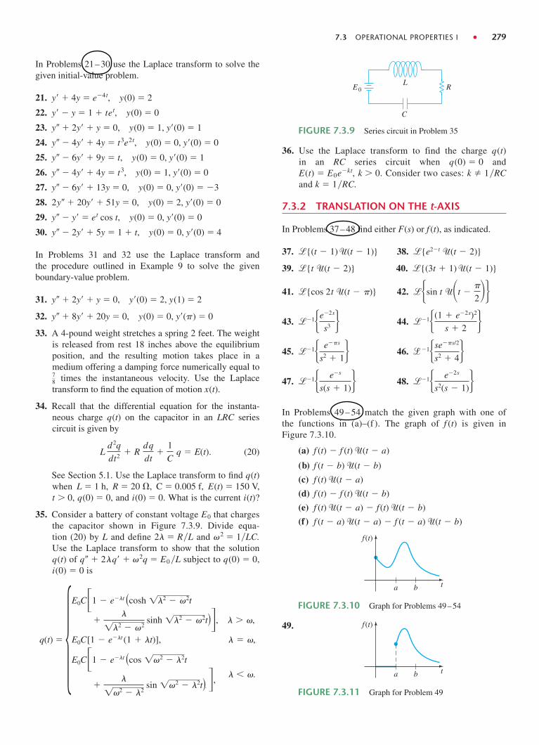
FIGURE 7.3.9 Series circuit in Problem 35
E0 R
C
L
FIGURE 7.3.10 Graph for Problems 49–54
t
f(t)
a b
49.
FIGURE 7.3.11 Graph for Problem 49
t
f(t)
a b
280 ● CHAPTER 7 THE LAPLACE TRANSFORM
FIGURE 7.3.12 Graph for Problem 50
t
f(t)
a b
FIGURE 7.3.13 Graph for Problem 51
t
f (t)
a b
FIGURE 7.3.14 Graph for Problem 52
t
f(t)
a b
FIGURE 7.3.15 Graph for Problem 53
t
f(t)
a b
FIGURE 7.3.16 Graph for Problem 54
t
f(t)
a b
50.
51.
52.
53.
54.
In Problems 55–62 write each function in terms of unit stepfunctions. Find the Laplace transform of the given function.
55.
56.
57. f (t) � �0,
t2,
0 � t � 1
t � 1
f (t) � �1,
0,
1,
0 � t � 4
4 � t � 5
t � 5
f (t) � �2,
�2,
0 � t � 3
t � 3
58.
59.
60. f (t) � �sin t,
0,
0 � t � 2�
t � 2�
f (t) � � t,
0,
0 � t � 2
t � 2
f (t) � �0,
sin t,
0 � t � 3�>2 t � 3�>2
61.
62.
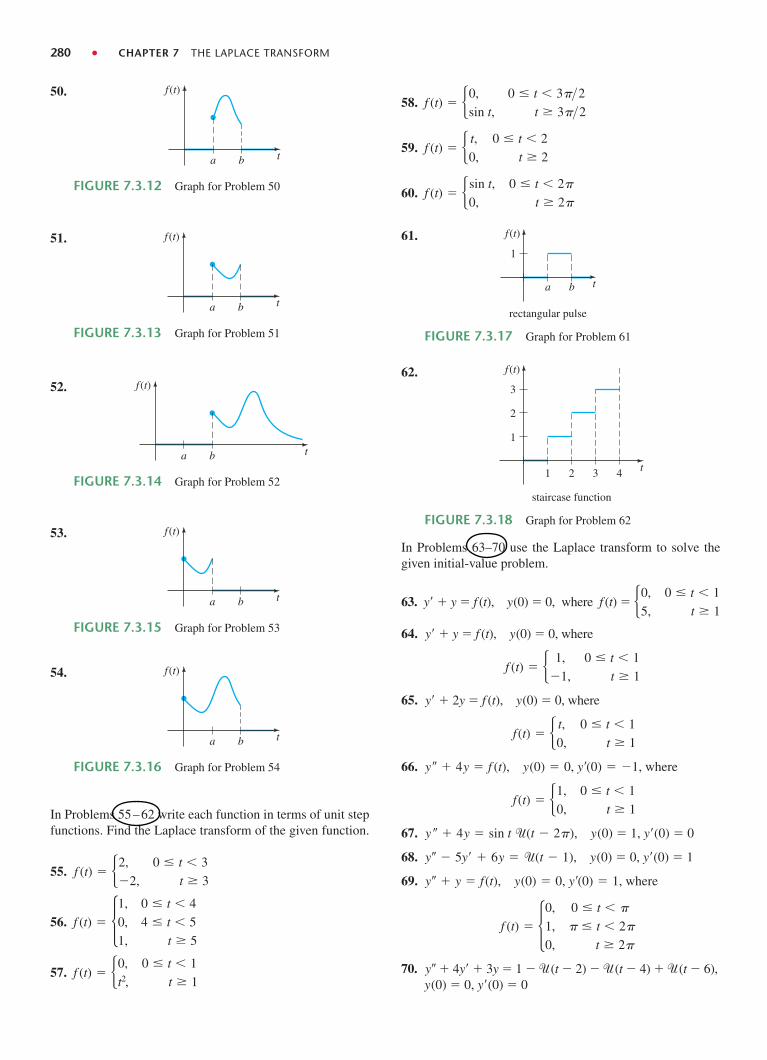
FIGURE 7.3.18 Graph for Problem 62
3
2
1
staircase function
t
f(t)
1 2 3 4
FIGURE 7.3.17 Graph for Problem 61
1
rectangular pulse
tba
f(t)
In Problems 63–70 use the Laplace transform to solve thegiven initial-value problem.
63. y� � y � f (t), y(0) � 0, where f (t) �
64. y� � y � f (t), y(0) � 0, where
65. y� � 2y � f (t), y(0) � 0, where
66. where
67. , y(0) � 1, y�(0) � 0
68. , y(0) � 0, y�(0) � 1
69. where
70. y � 4y� � 3y � 1 � �(t � 2) � �(t � 4) � �(t � 6),y(0) � 0, y�(0) � 0
f (t) � �0,
1,
0,
0 � t � �
� � t � 2�
t � 2�
y � y � f(t), y(0) � 0, y�(0) � 1,
y � 5y� � 6y � �(t � 1)
y � 4y � sin t �(t � 2�)
f(t) � �1,
0,
0 � t � 1
t � 1
y � 4y � f (t), y(0) � 0, y�(0) � �1,
f(t) � � t,
0,
0 � t � 1
t � 1
f (t) � � 1,
�1,
0 � t � 1
t � 1
�0,
5,
0 � t � 1
t � 1
7.4 OPERATIONAL PROPERTIES II ● 289
From
we can then rewrite (13) as
1
s(s � R>L)�
L>Rs
�L>R
s � R>L
.�1
R �1
s�
e�s
s�
e�2s
s�
e�3s
s� � �
1
R �1
s � R>L �1
s � R>L e�s �e�2s
s � R>L �e�3s
s � R>L � �
I(s) �1
R �1
s�
1
s � R>L�(1 � e�s � e�2s � e�3s � )
By applying the form of the second translation theorem to each term of both series,we obtain
�1
R(e�Rt/L � e�R(t�1)/L �(t � 1) � e�R(t�2)/L �(t � 2) � e�R(t�3)/L �(t � 3) � )
i(t) �1
R(1 � �(t � 1) � �(t � 2) � �(t � 3) � )
or, equivalently,
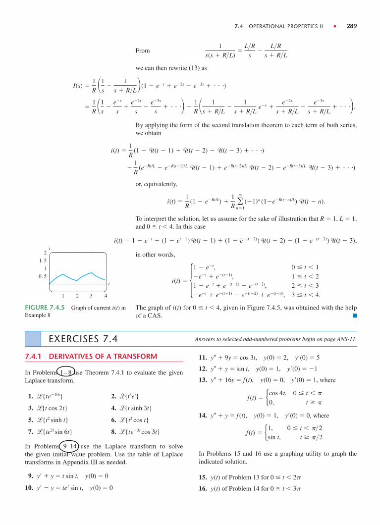
To interpret the solution, let us assume for the sake of illustration that R � 1, L � 1,and 0 � t � 4. In this case
i(t) �1
R(1 � e�Rt/L) �
1
R �
n�1(�1)n (1�e�R(t�n)/L) �(t � n).
;i(t) � 1 � e�t � (1 � et�1) �(t � 1) � (1 � e�(t�2)) �(t � 2) � (1 � e�(t�3)) �(t � 3)
in other words,
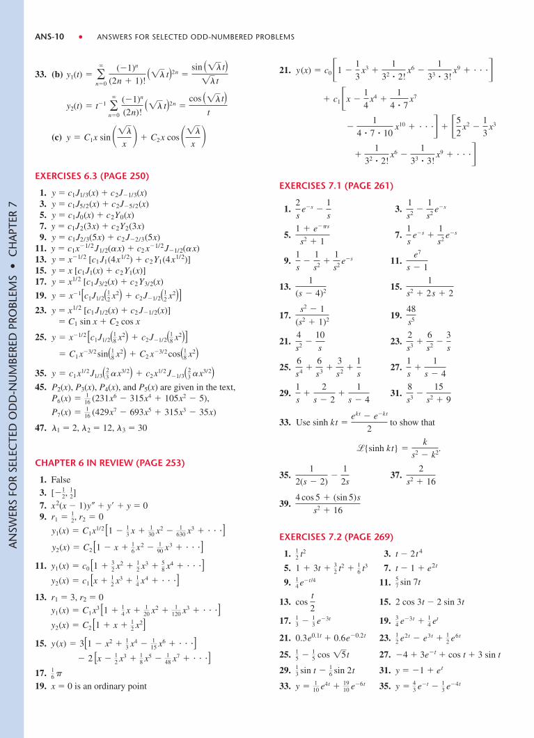
The graph of i(t) for 0 � t � 4, given in Figure 7.4.5, was obtained with the helpof a CAS.
i(t) � �1 � e�t,
�e�t � e�(t�1),
1 � e�t � e�(t�1) � e�(t�2),
�e�t � e�(t�1) � e�(t�2) � e�(t�3),
0 � t � 1
1 � t � 2
2 � t � 3
3 � t � 4.21 3 4
21.5
10.5
t
i
FIGURE 7.4.5 Graph of current i(t) inExample 8
EXERCISES 7.4 Answers to selected odd-numbered problems begin on page ANS-11.
7.4.1 DERIVATIVES OF A TRANSFORM
In Problems 1–8 use Theorem 7.4.1 to evaluate the givenLaplace transform.
1. 2.
3. 4.
5. 6.
7. 8.
In Problems 9–14 use the Laplace transform to solvethe given initial-value problem. Use the table of Laplacetransforms in Appendix III as needed.
9. y� � y � t sin t, y(0) � 0
10. y� � y � tet sin t, y(0) � 0
�{te�3t cos 3t}�{te2t sin 6t}
�{t2 cos t}�{t2 sinh t}
�{t sinh 3t}�{t cos 2t}
�{t3et}�{te�10t}
11. y � 9y � cos 3t, y(0) � 2, y�(0) � 5
12. y � y � sin t, y(0) � 1, y�(0) � �1
13. y � 16y � f (t), y(0) � 0, y�(0) � 1, where
14. y � y � f (t), y(0) � 1, y�(0) � 0, where
In Problems 15 and 16 use a graphing utility to graph theindicated solution.
15. y(t) of Problem 13 for 0 � t � 2p
16. y(t) of Problem 14 for 0 � t � 3p
f(t) � �1,
sin t,
0 � t � �>2 t � �>2
f(t) � �cos 4t,
0,
0 � t � �
t � �
290 ● CHAPTER 7 THE LAPLACE TRANSFORM
In some instances the Laplace transform can be used to solvelinear differential equations with variable monomial coeffi-cients. In Problems 17 and 18 use Theorem 7.4.1 to reducethe given differential equation to a linear first-order DEin the transformed function . Solve the first-order DE for Y(s) and then find .
17. ty � y� � 2t2, y(0) � 0
18. 2y � ty� � 2y � 10, y(0) � y�(0) � 0
7.4.2 TRANSFORMS OF INTEGRALS
In Problems 19–30 use Theorem 7.4.2 to evaluate the givenLaplace transform. Do not evaluate the integral beforetransforming.
19. 20.
21. 22.
23. 24.
25. 26.
27. 28.
29. 30.
In Problems 31–34 use (8) to evaluate the given inversetransform.
31. 32.
33. 34.
35. The table in Appendix III does not contain an entry for
.
(a) Use (4) along with the results in (5) to evaluate thisinverse transform. Use a CAS as an aid in evaluatingthe convolution integral.
(b) Reexamine your answer to part (a). Could you haveobtained the result in a different manner?
36. Use the Laplace transform and the results of Problem 35to solve the initial-value problem
.
Use a graphing utility to graph the solution.
y � y � sin t � t sin t, y(0) � 0, y�(0) � 0
� �1� 8k3s
(s2 � k2)3�
� �1� 1
s(s � a)2�� �1� 1
s3(s � 1)�
� �1� 1
s2(s � 1)�� �1� 1
s(s � 1)�
��t �t
0' e�' d'���t �t
0sin' d'�
���t
0sin ' cos (t � ') d'����t
0' et�' d'�
���t
0' sin ' d'����t
0e�' cos ' d'�
���t
0cos ' d'����t
0e' d'�
�{e2t � sin t}�{e�t � et cos t}
�{t2 � tet}�{1 � t3}
y(t) � � �1{Y(s)}Y(s) � �{y(t)}
In Problems 37–46 use the Laplace transform to solve thegiven integral equation or integrodifferential equation.
37.
38.
39.
40.
41.
42.
43.
44.
45.
46.
In Problems 47 and 48 solve equation (10) subject to i(0) � 0with L, R, C, and E(t) as given. Use a graphing utility to graphthe solution for 0 � t � 3.
47. L � 0.1 h, R � 3 ", C � 0.05 f,
48. L � 0.005 h, R � 1 ", C � 0.02 f,
7.4.3 TRANSFORM OF A PERIODICFUNCTION
In Problems 49–54 use Theorem 7.4.3 to find the Laplacetransform of the given periodic function.
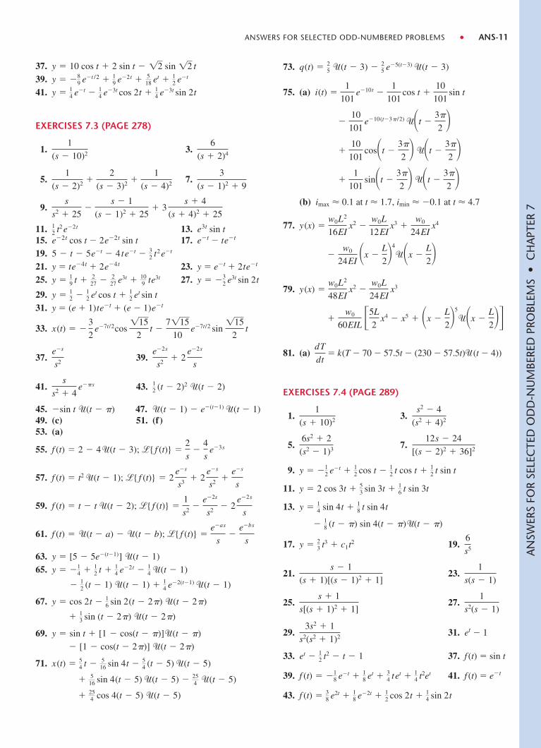
49.
E(t) � 100[t � (t � 1)�(t � 1)]
E(t) � 100[�(t � 1) � �(t � 2)]
dy
dt� 6y(t) � 9 �t
0y(') d' � 1, y(0) � 0
y�(t) � 1 � sin t � �t
0y(') d', y(0) � 0
t � 2 f (t) � �t
0(e' � e�' ) f (t � ') d'
f (t) � 1 � t �8
3�t
0(' � t)3 f (') d'
f (t) � cos t � �t
0e�'
f (t � ') d'
f (t) � �t
0f (') d' � 1
f (t) � 2 �t
0f (') cos (t � ') d' � 4e�t � sin t
f (t) � tet � �t
0' f (t � ') d'
f (t) � 2t � 4 �t
0sin ' f (t � ') d'
f (t) � �t
0(t � ') f (') d' � t
FIGURE 7.4.6 Graph for Problem 49
1
meander function
t2aa
f(t)
3a 4a
1
. (7)
The inverse form of (7),
, (8)�t
0f(') d' � � �1�F(s)
s �
���t
0f(') d'� �
F(s)
s
convolução
7.4 OPERATIONAL PROPERTIES II ● 291
57. , b � 1, k � 5, f is the meander function inProblem 49 with amplitude 10, and a � p, 0 � t � 2p.
58. m � 1, b� 2, k � 1, f is the square wave in Problem 50with amplitude 5, and a � p, 0 � t � 4p.
Discussion Problems
59. Discuss how Theorem 7.4.1 can be used to find
.
60. In Section 6.3 we saw that ty � y� � ty � 0 is Bessel’sequation of order n� 0. In view of (22) of that sectionand Table 6.1 a solution of the initial-value problemty � y� � ty � 0, y(0) � 1, y�(0) � 0, is y � J0(t). Usethis result and the procedure outlined in the instructionsto Problems 17 and 18 to show that
.
[Hint: You might need to use Problem 46 inExercises 7.2.]
61. (a) Laguerre’s differential equation
ty � (1 � t)y� � ny � 0
is known to possess polynomial solutions when n isa nonnegative integer. These solutions are naturallycalled Laguerre polynomials and are denoted byLn(t). Find y � Ln(t), for n � 0, 1, 2, 3, 4 if it isknown that Ln(0) � 1.
(b) Show that
,
where and y � Ln(t) is a polynomialsolution of the DE in part (a). Conclude that
.
This last relation for generating the Laguerre poly-nomials is the analogue of Rodrigues’ formula forthe Legendre polynomials. See (30) in Section 6.3.
Computer Lab Assignments
62. In this problem you are led through the commands inMathematica that enable you to obtain the symbolicLaplace transform of a differential equation and the so-lution of the initial-value problem by finding the inversetransform. In Mathematica the Laplace transform ofa function y(t) is obtained using LaplaceTransform[y[t], t, s]. In line two of the syntax we replaceLaplaceTransform [y[t], t, s] by the symbol Y. (If youdo not have Mathematica, then adapt the given proce-dure by finding the corresponding syntax for the CASyou have on hand.)
Ln(t) �et
n!
dn
dtn tne�t, n � 0, 1, 2, . . .
Y(s) � �{y}
��et
n!
dn
dtn tne�t� � Y(s)
�{J0(t)} �1
1s2 � 1
� �1�lns � 3
s � 1�
m � 12
FIGURE 7.4.7 Graph for Problem 50
FIGURE 7.4.8 Graph for Problem 51
FIGURE 7.4.9 Graph for Problem 52
FIGURE 7.4.10 Graph for Problem 53
1
square wave
t2aa
f(t)
3a 4a
sawtooth function
t2bb
a
f(t)
3b 4b
1
triangular wave
t2
f(t)
3 41
1
full-wave rectification of sin t
t
f(t)
432π π π π
50.
51.
52.
53.
FIGURE 7.4.11 Graph for Problem 54
432π π π π
1
half-wave rectification of sin t
t
f(t)54.
In Problems 55 and 56 solve equation (12) subject toi(0) � 0 with E(t) as given. Use a graphing utility to graphthe solution for 0 � t � 4 in the case when L � 1 and R � 1.
55. E(t) is the meander function in Problem 49 withamplitude 1 and a � 1.
56. E(t) is the sawtooth function in Problem 51 withamplitude 1 and b � 1.
In Problems 57 and 58 solve the model for a drivenspring/mass system with damping
where the driving function f is as specified. Use a graphingutility to graph x(t) for the indicated values of t.
md 2x
dt2 � �dx
dt� kx � f (t), x(0) � 0, x�(0) � 0,
ANS-10 ● ANSWERS FOR SELECTED ODD-NUMBERED PROBLEMS
AN
SWER
S FO
R SE
LEC
TED
OD
D-N
UM
BERE
D P
ROBL
EMS
• C
HA
PTER
7
33. (b)
(c)
EXERCISES 6.3 (PAGE 250)
1. y � c1J1/3(x) � c2J�1/3(x)3. y � c1J5/2(x) � c2J�5/2(x)5. y � c1J0(x) � c2Y0(x)7. y � c1J2(3x) � c2Y2(3x)9. y � c1J2/3(5x) � c2J�2/3(5x)
11. y � c1x�1/2J1/2(ax) � c2 x�1/2J�1/2(ax)13. y � x�1/2 [c1J1(4x1/2) � c2Y1(4x1/2)]15. y � x [c1J1(x) � c2Y1(x)]17. y � x1/2 [c1J3/2(x) � c2Y3/2(x)
19.
23. y � x1/2 [c1J1/2(x) � c2 J�1/2(x)]� C1 sin x � C2 cos x
25.
35.
45. P2(x), P3(x), P4(x), and P5(x) are given in the text,,
47. l1 � 2, l2 � 12, l3 � 30
CHAPTER 6 IN REVIEW (PAGE 253)
1. False
3.7. x2(x � 1)y � y� � y � 09.
11.
13. r1 � 3, r2 � 0
15.
17.19. x � 0 is an ordinary point
16 �
� 2 [x � 12 x3 � 1
8 x5 � 148 x7 � ]
y(x) � 3[1 � x2 � 13 x4 � 1
15 x6 � ]y2(x) � C2 [1 � x � 1
2 x2]y1(x) � C1x3 [1 � 1
4 x � 120 x2 � 1
120 x3 � ]
y2(x) � c1 [x � 12 x3 � 1
4 x4 � ]y1(x) � c0 [1 � 3
2 x2 � 12 x3 � 5
8 x4 � ]y2(x) � C2 [1 � x � 1
6 x2 � 190 x3 � ]
y1(x) � C1x1/2 [1 � 13 x � 1
30 x2 � 1630 x3 � ]
r1 � 12, r2 � 0
[�12,
12]
P7(x) � 116 (429x7 � 693x5 � 315x3 � 35x)
P6(x) � 116 (231x6 � 315x4 � 105x2 � 5)
y � c1x1/2J1/3(23 ax3/2) � c2x1/2J�1/3(2
3 ax3/2)� C1x�3/2sin(1
8 x2) � C2 x�3/2 cos(18 x2)
y � x�1/2 [c1J1/2(18 x2) � c2J�1/2(1
8 x2)]
y � x�1[c1J1/2(12 x2) � c2J�1/2(1
2 x2)]
y � C1x sin �1�
x � � C2x cos �1�
x �
y2(t) � t�1 �
n�0
(�1)n
(2n)!(1� t)2n �
cos (1� t)
t
y1(t) � �
n�0
(�1)n
(2n � 1)!(1� t)2n �
sin (1� t)1�
t21.
EXERCISES 7.1 (PAGE 261)
1. 3.
5. 7.
9. 11.
13. 15.
17. 19.
21. 23.
25. 27.
29. 31.
33. Use sinh to show that
35. 37.
39.
EXERCISES 7.2 (PAGE 269)
1. 3. t � 2t4
5. 7. t � 1 � e2t
9. 11.
13. 15. 2 cos 3t � 2 sin 3t
17. 19.
21. 0.3e0.1t � 0.6e�0.2t 23.
25. 27. �4 � 3e�t � cos t � 3 sin t
29. 31. y � �1 � et
33. 35. y � 43 e�t � 1
3 e�4ty � 110 e4t � 19
10 e�6t
13 sin t � 1
6 sin 2t
15 � 1
5 cos 15t
12 e2t � e3t � 1
2 e6t
34 e�3t � 1
4 et13 � 1
3 e�3t
cost
2
57 sin 7t1
4 e�t/4
1 � 3t � 32 t2 � 1
6 t3
12 t2
4 cos 5 � (sin 5)s
s2 � 16
2
s2 � 16
1
2(s � 2)�
1
2s
�{sinh kt} �k
s2 � k2.
kt �ekt � e�kt
2
8
s3 �15
s2 � 9
1
s�
2
s � 2�
1
s � 4
1
s�
1
s � 4
6
s4 �6
s3 �3
s2 �1
s
2
s3 �6
s2 �3
s
4
s2 �10
s
48
s5
s2 � 1
(s2 � 1)2
1
s2 � 2s � 2
1
(s � 4)2
e7
s � 1
1
s�
1
s2 �1
s2 e�s
1
se�s �
1
s2 e�s1 � e��s
s2 � 1
1
s2 �1
s2 e�s2
se�s �
1
s
�1
32 � 2!x6 �
1
33 � 3!x9 � �
�1
4 � 7 � 10x10 � � � 5
2x2 �
1
3x3
� c1x �1
4x4 �
1
4 � 7x7
y(x) � c01 �1
3x3 �
1
32 � 2!x6 �
1
33 � 3!x9 � �
ANSWERS FOR SELECTED ODD-NUMBERED PROBLEMS ● ANS-11
AN
SWER
S FO
R SE
LEC
TED
OD
D-N
UM
BERE
D P
ROBL
EMS
• C
HA
PTER
7
37.39.41.
EXERCISES 7.3 (PAGE 278)
1. 3.
5. 7.
9.
11. 13. e3t sin t15. e�2t cos t � 2e�2t sin t 17. e�t � te�t
19.21. y � te�4t � 2e�4t 23. y � e�t � 2te�t
25. 27.
29.31. y � (e � 1)te�t � (e � 1)e�t
33.
37. 39.
41. 43.
45. 47.49. (c) 51. (f)53. (a)
55.
57.
59.
61.
63.65.
67.
69.
71.
� 254 cos 4(t � 5) �(t � 5)
� 516 sin 4(t � 5) �(t � 5) � 25
4 �(t � 5)
x(t) � 54 t � 5
16 sin 4t � 54 (t � 5) �(t � 5)
� [1 � cos(t � 2�)] �(t � 2�)
y � sin t � [1 � cos(t � �)]�(t � �)
� 13 sin (t � 2�) �(t � 2�)
y � cos 2t � 16 sin 2(t � 2�) �(t � 2�)
� 12 (t � 1) �(t � 1) � 1
4 e�2(t�1) �(t � 1)
y � �14 � 1
2 t � 14 e�2t � 1
4 �(t � 1)
y � [5 � 5e�(t�1)] �(t � 1)
f (t) � �(t � a) � �(t � b); �{ f (t)} �e�as
s�
e�bs
s
f (t) � t � t �(t � 2); �{ f (t)} �1
s2 �e�2s
s2 � 2e�2s
s
f (t) � t2 �(t � 1); �{ f (t)} � 2e�s
s3 � 2e�s
s2 �e�s
s
f (t) � 2 � 4�(t � 3); �{ f (t)} �2
s�
4
se�3s
�(t � 1) � e�(t�1) �(t � 1)�sin t �(t � �)
12 (t � 2)2 �(t � 2)
s
s2 � 4e��s
e�2s
s2 � 2e�2s
s
e�s
s2
x(t) � �3
2e�7t/2cos
115
2t �
7115
10e�7t/2 sin
115
2t
y � 12 � 1
2 et cos t � 12 et sin t
y � �32 e3t sin 2ty � 1
9 t � 227 � 2
27 e3t � 109 te3t
5 � t � 5e�t � 4 te�t � 32 t2 e�t
12 t2 e�2t
s
s2 � 25�
s � 1
(s � 1)2 � 25� 3
s � 4
(s � 4)2 � 25
3
(s � 1)2 � 9
1
(s � 2)2 �2
(s � 3)2 �1
(s � 4)2
6
(s � 2)4
1
(s � 10)2
y � 14 e�t � 1
4 e�3t cos 2t � 14 e�3t sin 2t
y � �89 e�t /2 � 1
9 e�2t � 518 et � 1
2 e�t
y � 10 cos t � 2 sin t � 12 sin 12 t 73.
75. (a)
(b) imax 0.1 at t 1.7, imin �0.1 at t 4.7
77.
79.
81. (a) � k(T � 70 � 57.5t � (230 � 57.5t)�(t � 4))
EXERCISES 7.4 (PAGE 289)
1. 3.
5. 7.
9.
11.
13.
17. 19.
21. 23.
25. 27.
29. 31. et � 1
33. 37. f (t) � sin t
39. 41. f (t) � e�t
43. f (t) � 38 e2t � 1
8 e�2t � 12 cos 2t � 1
4 sin 2t
f (t) � �18 e�t � 1
8 et � 34 tet � 1
4 t2et
et � 12 t2 � t � 1
3s2 � 1
s2(s2 � 1)2
1
s2(s � 1)
s � 1
s[(s � 1)2 � 1]
1
s(s � 1)
s � 1
(s � 1)[(s � 1)2 � 1]
6
s5y � 23 t3 � c1t2
� 18 (t � �) sin 4(t � �)�(t � �)
y � 14 sin 4t � 1
8 t sin 4t
y � 2 cos 3t � 53 sin 3t � 1
6 t sin 3t
y � �12 e�t � 1
2 cos t � 12 t cos t � 1
2 t sin t
12s � 24
[(s � 2)2 � 36]2
6s2 � 2
(s2 � 1)3
s2 � 4
(s2 � 4)2
1
(s � 10)2
dT
dt
�w0
60EIL 5L
2x4 � x5 � �x �
L
2�5
��x �L
2��
y(x) �w0L2
48EIx2 �
w0L
24EIx3
�w0
24EI �x �L
2�4
��x �L
2�
y(x) �w0L2
16EIx2 �
w0L
12EIx3 �
w0
24EIx4
�1
101sin�t �
3�
2 � ��t �3�
2 �
�10
101cos�t �
3�
2 � ��t �3�
2 �
�10
101e�10(t�3�/2) ��t �
3�
2 �
i(t) �1
101e�10t �
1
101cos t �
10
101sin t
q(t) � 25 �(t � 3) � 2
5 e�5(t�3) �(t � 3)
ANS-12 ● ANSWERS FOR SELECTED ODD-NUMBERED PROBLEMS
AN
SWER
S FO
R SE
LEC
TED
OD
D-N
UM
BERE
D P
ROBL
EMS
• C
HA
PTER
7
45.
47.
49.
51.
53.
55.
57.
EXERCISES 7.5 (PAGE 295)
1.
3.
5.
7.
9.
11.
13.
EXERCISES 7.6 (PAGE 299)
1. 3.
5. 7.
9.
11.
y � �13 � 1
3 e�t � 13 te�t
x � 12 t2 � t � 1 � e�t
y � �2
3!t3 �
1
4!t 4
x � 8 �2
3!t3 �
1
4!t 4
y � �12 t � 3
4 12 sin 12 ty � 83 e3t � 5
2 e2t � 16
x � �12 t � 3
4 12 sin 12 tx � �2e3t � 52 e2t � 1
2
y � 2 cos 3t � 73 sin 3ty � 1
3 e�2t � 23 et
x � �cos 3t � 53 sin 3tx � �1
3 e�2t � 13 et
y(x) � �P0
EI �L
4x2 �
1
6x3�, 0 � x �
L
2
P0L2
4EI �1
2x �
L
12�, L
2� x � L
� 13 e�2(t�3�) sin 3(t � 3�) �(t � 3�)
� 13 e�2(t��) sin 3(t � �) �(t � �)
y � e�2t cos 3t � 23 e�2t sin 3t
y � e�2(t�2�) sin t �(t � 2�)
y � 12 � 1
2 e�2t � [12 � 1
2 e�2(t�1)] �(t � 1)
y � �cos t �(t � �2) � cos t �(t � 3�
2 )y � sin t � sin t �(t � 2�)
y � e3(t�2) �(t � 2)
� 13 e�(t�n�) sin 3(t � n�)]�(t � n�)
� 4 �
n�1(�1)n [1 � e�(t�n�) cos 3(t � n�)
x(t) � 2(1 � e�t cos 3t � 13 e�t sin 3t)
�2
R �
n�1(�1)n (1 � e�R(t�n)/L)�(t � n)
i(t) �1
R(1 � e�Rt/L)
coth (�s>2)
s2 � 1
a
s �1
bs�
1
ebs � 1�
1 � e�as
s(1 � e�as)
� 100[e�10(t�2) � e�20(t�2)]�(t � 2)
i(t) � 100[e�10(t�1) � e�20(t�1)]�(t � 1)
y(t) � sin t � 12 t sin t
13.
15. (b)
(c) i1 � 20 � 20e�900t
17.
19.
CHAPTER 7 IN REVIEW (PAGE 300)
1. 3. false
5. true 7.
9. 11.
13. 15.
17.
19.
21. �5 23. e�k(s�a)F(s � a)
25. 27.
29. ;
;
31. ;
;
33.
35.
37.
39.
y � t � 94 e�2t � 1
4 e2t
x � �14 � 9
8 e�2t � 18 e2t
y � 1 � t � 12 t2
� 9100 e�5(t�2) �(t � 2)
� 15 (t � 2) �(t � 2) � 1
4 e�(t�2) �(t � 2)
y � � 625 � 1
5 t � 32 e�t � 13
50 e�5t � 425 �(t � 2)
y � 5tet � 12 t2 et
�{et f (t)} �2
s � 1�
1
(s � 1)2 e�2(s�1)
�{ f (t)} �2
s�
1
s2 e�2s
f (t) � 2 � (t � 2) �(t � 2)
�1
s � 1e�4(s�1)
�{et f (t)} �1
(s � 1)2 �1
(s � 1)2 e�(s�1)
�{ f (t)} �1
s2 �1
s2 e�s �1
se�4s
f (t) � t � (t � 1)�(t � 1) � �(t � 4)
f (t � t0)�(t � t0)f (t)�(t � t0)
cos � (t � 1)�(t � 1) � sin � (t � 1)�(t � 1)
e5t cos 2t � 52 e5t sin 2t
12 t2 e5t1
6 t5
4s
(s2 � 4)2
2
s2 � 4
1
s � 7
1
s2 �2
s2 e�s
i2 �6
5�
6
5e�100t cosh 5012 t �
612
5e�100t sinh 5012 t
i1 �6
5�
6
5e�100t cosh 5012 t �
912
10e�100t sinh 5012 t
i3 � 3013 e
�2t � 2501469 e
�15t � 280113 cos t � 810
113 sin t
i2 � �2013 e
�2t � 3751469 e
�15t � 145113 cos t � 85
113 sin t
i3 � 809 � 80
9 e�900t
i2 � 1009 � 100
9 e�900t
x2 �2
5 sin t �
16
15 sin 16 t �
4
5 cos t �
1
5 cos 16 t
x1 �1
5 sin t �
216
15sin 16 t �
2
5 cos t �
2
5 cos 16 t