APPENDIX

COMPUTER SIMULATION EXERCISES

M. P. ALLEN H. H. Wills Physics Laboratory

Royal Fort, Tyndall Avenue, Bristol BS8 1 TL D. M. HEYES

Department of Chemistry Royal Holloway and Bedford New College, Egham, Surrey

M. LESLIE TCS Division

SERC Daresbury Laboratory, Daresbury, Warrington WA4 4AD S. L. PRICE

University Chemical Laboratory Lensfield Road, Cambridge CB2 lEW

W. SMITH TCS Division

SERC Daresbury Laboratory, Daresbury, Warrington WA4 4AD D. J. TILDESLEY

Department of Chemistry The University, Southampton S09 5NH

Abstract

We present an overview of methods and applications of computer simula­tions in the field of fluids, polymers, and solids, through a set of exercises and projects. These exercises were actually undertaken by students attending the Advanced Study Institute: most involve access to a computer, but some require pen and paper only.

1 Introduction

A set of exercises, intended to give the students 'hands-on' experience of computer modelling techniques, formed an integral part of the Advanced Study Institute. In­struction sheets were made available to the participants, who were each allocated a

431

C.RA. Cat/ow et al. (eds.), Computer Modelling of Fluids Polymers and Solids, 431-536. © 1990 by Kluwer Academic Publishers.

432

user identifier on the Bath University mainframe computer. A brief introduction to the essentials of the operating system was given, together with information regarding the compiling and running of FORTRAN programs, the linking of numerical libraries, plotting facilities, etc. The problems classes themselves were conducted in the after­noons, with the authors and local experts on hand to give assistance and guidance where required, but access to the computer was fairly free, and some keen students worked well into the evenings!

Here we reproduce the instructions, modified only slightly from the originals. Some problems involved accessing files on the computer provided by the authors. We have had to omit these for reasons of space; nonetheless, the essentials of the problem should be clear in each case. Each problem was given a 'star' rating according to degree of difficulty: introductory exercises were rated '*' while small projects (perhaps suitable for a team) were rated '*****'.

Here is a complete list of problems, grouped together by general subject area, with their authors identified by initials, and the degree of difficulty indicated. The numbers indicate sections within this chapter.

The first set of introductory exercises do not involve extensive programming; in some cases, they merely require pen and paper.

2 Long-range corrections and power-law potentials * (dmh)

3 Permanent electrostatic interactions * (djt)

4 To demonstrate the differences between simple electrostatic models ** (sIp)

5 Lennard-Jones lattice energies ** (mpa)

6 Ionic crystal energy calculations. Direct summation ** (ml)

7 Lennard-Jones Monte Carlo ** (mpa)

8 Lennard-Jones molecular dynamics ** (djt)

9 Monte Carlo by hand * (mpa)

These are followed by some tasks involving the modification, writing, and running, of simulation programs.

10 Hard sphere Monte Carlo in one dimension * * * (djt)

11 Hard sphere dynamics in one dimension *** (mpa)

12 A Monte Carlo simulation of Lennard-Jones atoms in one dimension *** (djt)

13 Ising model simulations **** (mpa)

The third group of exercises concern the development of realistic intermolecular po­tentials.

433

14 The effects of small non-sphericities in the model atom-atom intermolecular potential on the predicted crystal structure of an A2 molecule ** (sIp)

15 Deriving a model potential for CS2 by fitting to the low temperature crystal structure ** (sIp)

This is followed by a series of problems highlighting a variety of interesting applica­tions of simulation.

16 The Lennard-Jones fluid: a hard-sphere fluid in disguise? *** (dmh)

17 Time correlation functions ** (djt)

18 Polymer reptation Monte Carlo *** (mpa)

19 Simulations of crystal surfaces * * * (mpa)

20 Irreversible aggregation by Brownian dynamics simulation * * * (dmh)

21 Diffusion-limited aggregation * * ** (djt)

22 Shear flow in 2d Lennard-Jones fluid by non-equilibrium molecular dynamics

**** (dmh)

The next four exercises deal with applications of the Fourier transform: they are preceded by an introductory section.

23 The Fourier transform and applications to molecular dynamics (ws)

24 Harmonic analysis * (ws)

25 Correlation functions ** (ws)

26 Particle density calculations ** (ws)

27 Quantum simulations * * * (ws)

Finally, there is a set of rather more substantial projects.

28 Percolation cluster statistics of ID fluids * * ** (dmh)

29 Quaternions and constraints * * * * * (mpa)

30 The chemical potential of liquid butane * * * * * (djt)

31 Molecular dynamics on the Distributed Array Processor ***** (mpa)

434

2 Long-range corrections and power-law poten­tials

2.1 Summary

The long-range correction to the internal energy and the virial can have important consequences in many areas of simulation. This is a pen-and-paper exercise to give you practice at working out some of these expressions.

2.2 Background

Let us consider a monatomic fluid or crystal in which the particles interact through a simple pair potential of the form

¢( 7') = t( (j / 7' t , (2.1)

where 7' is the separation between the two particles, n is usually an integer (positive), t

is a characteristic energy and (j is a characteristic "molecular" diameter. The internal energy, U, and pressure, P, in a simulation are defined by

N-l N

U = L L ¢(7'ij) (2.2) i=1 j>i

and

P = ~(~m.r? - w) 3V ~ " , .=1

(2.3)

where W is the so-called virial,

,T. _ ~1 ~ .. d¢(7'ij) ~ - L.J L.J 7"3 •

i=1 j>i d7' (2.4)

In these expressions p = N (j3 /V, where N is the number of particles in a simulation cell of volume V. The mass of particle i is mi. ri is the position of particle ij ri = drddt, rij = ri - rj'

In any simulation it is necessary to truncate pair-interactions beyond some spec­ified pair separation distance, which we will denote by 7'c' Short range potentials, n > 1, are normally truncated at several (j and certainly 7' < V 1 / 3 /2 for a cubic unit cell, or half the minimum sidelength for a non-cubic simulation cell - so that the par­ticle only interacts with one image of another particle. Therefore the contributions to eqns (2.2) - (2.4) for those interactions for which 7'ij > 7'c are set to zero. An estimate of the effect of these neglected interactions can be made by assuming that

435

there is a "smeared-out" distribution of molecules for rij > rc of density p. These long-range corrections to the internal energy and virial in three dimensions are:

(2.5)

and

100 3d¢(r) Wlrc = 27rp r --dr.

rc dr (2.6)

In eqns (2.5) and (2.6) we have assumed that the pair radial distribution function, g(r) = 1,r > rc.

2.3 The problem

The object of this exercise is to evaluate expressions for the long range corrections to the energy and pressure for potentials ¢(r) = €(u/r)n in 1,2 and 3 dimensions. Take the truncation distance to be rc. Assume that the pair distribution function is unity for pair separations r > rc.

2.4 Further tasks

• Is the long-range correction larger for the internal energy or the pressure?

• By inspection discover the smallest value of n one can use in each dimension, without having summation convergence problems.

• Are eqns (2.5) and (2.6) also valid for a crystal simulation?

3 Permanent electrostatic interactions

3.1 Summary

This problem offers some exercises on modelling permanent electrostatic interactions for use in simulations. In the main these problems can be tackled using pencil and paper, but you will need to resort to the computer from time to time.

3.2 Background

There are three types of long-range intermolecular interactions which bind molecules together in condensed phases. All molecules interact through an attractive dispersion potential. This arises from the coupling between an induced-dipole on one molecule and an induced-dipole on a neighbour. The interaction falls off with the inverse sixth power of the intermolecular separation. It is approximately pairwise additive, gen­erally anisotropic, and increases with increasing molecular polarizability. It is the

436

dominant attractive interaction in many condensed phases e.g. liquid N2 and solid CS2 • A less important interaction is that due to induction. For instance, the elec­trostatic dipole in HCI creates a field at a neighbouring molecule which couples with the polarizability to produce a temporary dipole in a neighbour. The induced and permanent dipole attract. This interaction is not pairwise additive and is normally small if the molecule is in a reasonably symmetrical environment such as provided by the solid or liquid. The permanent electrostatic interactions arise from the cou­pling of the charge distributions. The lowest non-zero electrostatic moment depends on the symmetry of the molecule: for a heteronuclear diatomic such as CO, the lowest non-zero moment is a dipole; for a homonuclear diatomic such as O2 it is a quadrupole, and for a tetrahedral molecule such as CH4 it is an octopole. These interactions are usually anisotropic, exactly pairwise additive, and can be attractive or repulsive. In computer simulations of solids and liquids, the electrostatic interac­tions are normally added to the core of the molecule. This core might be the three Lennard-Jones sites in a model of CO2 which provide the anisotropic dispersion and repulsion between molecules. The electrostatic potential is added to the core in one of three ways. We can represent the charge distribution as a set of point electrostatic moments located at the centre of mass of each molecule. For two CO molecules the first term in the series will be the dipole-dipole interaction which falls off as r- 3 •

The orientational dependence is a sum of first order spherical harmonics, and the strength of the interaction will depend on the square of the magnitude of the dipole moment. CO also has a sizeable quadrupole and the next terms in the series will be the dipole-quadrupole and the corresponding quadrupole-dipole interactions. The quadrupole-quadrupole interaction falls off as r- 5 , depends on second order spherical harmonics of the relative molecular orientations and the square of the magnitude of the quadrupole moment. There are many higher order terms and the series may not be rapidly convergent. It is certainly not convergent for intermolecular separations which are less than the length of the molecules. In an alternative description of the charge distribution the moments can always be represented by distributing partial charges inside the core of the molecule. These charges should produce the lowest non-zero moment and will also produce higher moments automatically. Even if th~ magnitude of the charges are chosen to fit the lowest moment, there is no certainty that these higher moments be the same size or sign as the experimentally measured values. A dipole requires a minimum of two charges and a quadrupole a minimum of three. The lowest moments can of course be represented by more charges and this gives some flexibility for fitting some of the higher moments, i.e. a useful model for water involves four charges distributed tetrahedrally to produce a dipole and tc mimic the lone pairs of electrons. These charge distributions can be unrealistic. FOl example, N2 has a negative quadrupole moment which can be modelled as two neg­ative charges, one on each atom, and a double positive charge at the centre of mas! of the molecule. However, chemical intuition tells us that there should be a builC: up of negative charge in the centre of the triple bond. Perhaps the most attractiv(

437

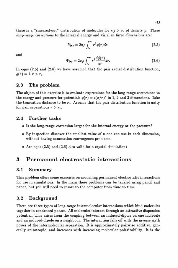
Figure 3.1: A configuration of CS2 molecules

I •••........ \

scheme is the use of a number of multi pole moments distributed at sites within the hard core. This approach has been pioneered by Stone and co-workers and can give an accurate and simple description of the complete charge distribution, which is more rapidly convergent than the traditional multipole expansion. An interesting example is chlorine where the overall charge distribution can be represented by a dipole and quadrupole situated on each of the atoms. There is not sufficient space in these notes to give any sort of description of the detail of these three techniques. However there are many useful references which give explicit formulae and a more detailed discus­sion of the problem [1,2,3,4]. The reader is also referred to appendix D of [2], which has a complete discussion of the units used to describe multipoles and charges, and a comprehensive list of experimentally and theoretically measured multipoles.

3.3 Task

The following problems are roughly in order of difficulty. It is not necessary to do them all. You can join in when the bar is at the right height .

• The quadrupole moment of CS 2 is 7 X 1O-4°Cm2 • The separation of the sulphur atoms is O.267nm. What charges (in units of the electronic charge) should be placed at the three nuclei to represent the quadrupole? Three CS2 molecules are arranged in a plane with their centres on the vertices of an equilateral triangle, as shown in the figure. If the centres of the molecules are separated by OAnm, what is the quadrupolar energy of the trimer?

• In a recent MD study of Cl2 , the charge distribution was described by placing a dipole and quadrupole on each of the chlorine atoms. The bondlength of the

438

molecule is 0.1994nm, the dipole is -0.1449 eao, and the quadrupole is 1.8902 ea~. (These moments are given in the usual atomic units). What are the quadrupole and hexadecapole moments of this molecule referred to its centre of mass. In a simulation of chlorine all interactions were cutoff at centre of mass separation of 0.35nm. What is the long-range correction to the electrostatic energy in this model?

• The lowest non-zero moment of CF4 is the octopole moment. The value ob­tained from collision induced adsorption studies is 4.0 X 1O-3esu cm3• Develop a five charge model for the electrostatic interaction between a pair of CF4

molecules. What is the most favourable orientation of the pair?

• The first four non-zero moments of nitrogen have been estimated using ab­initio methods: M2 = -1.041ea~; M4 = -6.600ea~; M6 = -15.44ea~; Ms = -29.40ea~. Develop a five charge model which describes this charge distribu­tion.

• The dipole moment of OCS is 0.7152 X lO-lSesu cm. The quadrupole moment is -2.0 X 10-26esu cm2 • If the higher order moments are zero, what is the favoured orientation of a pair of OCS molecules?

4 To demonstrate the differences between simple electrostatic models

4.1 Task

Model potentials for small molecules often include an electrostatic term which is designed to give the correct electrostatic energy at long range (molecular separation R » molecular dimensions) by ensuring that the model reproduces the experimental value for the first multipole moment. This can be done by either using the first central multipole moment in a one site model, or by using a set of point multipoles on every atomic site, or other choices of multiple interaction sites. The different choices can produce very different estimates of the electrostatic energy for smaller separations of the molecules, as they correspond to different implicit values of the higher multipole moments.

To demonstrate this, use the formulae below to derive (a) a point charge (Qoo) model with sites on each C and H atom, and (b) a distributed quadrupole (Q20) model with sites on just the carbon atoms, for acetylene (HCCH) and benzene (C6H6) which correspond to their central multipole moments Qfo = 5.46ea~ and Qfo = -7.22ea~ respectively (SCF values). What assumptions are these two models making about the form of the charge distributions of these molecules? Acetylene has the z axis along the molecule and the bondlengths are C-C 2.274 ao and C-H 2.004 ao. Benzene

439

has the z axis along the sixfold axis and the C-C and C-H bondlengths are 2.634 ao and 2.033 ao respectively.

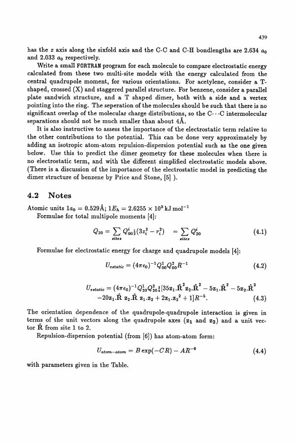
Write a small FORTRAN program for each molecule to compare electrostatic energy calculated from these two multi-site models with the energy calculated from the central quadrupole moment, for various orientations. For acetylene, consider a T­shaped, crossed (X) and staggered parallel structure. For benzene, consider a parallel plate sandwich structure, and a T shaped dimer, both with a side and a vertex pointing into the ring. The seperation of the molecules should be such that there is no significant overlap of the molecular charge distributions, so the C· . ·C intermolecular separations should not be much smaller than about 4A.

It is also instructive to assess the importance of the electrostatic term relative to the other contributions to the potential. This can be done very approximately by adding an isotropic atom-atom repulsion-dispersion potential such as the one given below. Use this to predict the dimer geometry for these molecules when there is no electrostatic term, and with the different simplified electrostatic models above. (There is a discussion of the importance of the electrostatic model in predicting the dimer structure of benzene by Price and Stone, [5) ).

4.2 Notes

Atomic units lao = 0.529A j 1Eh = 2.6255 X 103 kJ mol-1

Formulae for total multipole moments [4):

Formulae for electrostatic energy for charge and quadrupole models [4):

( 4.1)

(4.2)

The orientation dependence of the quadrupole-quadrupole interaction is given in terms of the unit vectors along the quadrupole axes (Zl and Z2) and a unit vec­tor R from site 1 to 2.

Repulsion-dispersion potential (from [6]) has atom-atom form:

Uatom-atom = B exp( -0 R) - AR-6 ( 4.4)

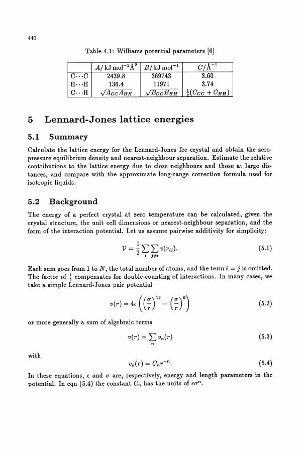
with parameters given in the Table.

440

Table 4.1: Williams potential parameters [6)

AI kJ mol-1 A I> BlkJmol-1 CIA -1

C···C 2439.8 369743 3.60 H .. ·H 136.4 11971 3.74 C···H JAccAHH JBcCBHH HCcc + CHH )

5 Lennard-J ones lattice energies

5.1 Summary

Calculate the lattice energy for the Lennard-Jones fcc crystal and obtain the zero­pressure equilibrium density and nearest-neighbour separation. Estimate the relative contributions to the lattice energy due to close neighbours and those at large dis­tances, and compare with the approximate long-range correction formula used for isotropic liquids.

5.2 Background

The energy of a perfect crystal at zero temperature can be calculated, given the crystal structure, the unit cell dimensions or nearest-neighbour separation, and the form of the interaction potential. Let us assume pairwise additivity for simplicity:

(5.1)

Each sum goes from 1 to N, the total number of atoms, and the term i = j is omitted. The factor of ! compensates for double-counting of interactions. In many cases, we take a simple Lennard-Jones pair potential

(5.2)

or more generally a sum of algebraic terms

(5.3) n

with (5.4)

In these equations, € and (j are, respectively, energy and length parameters in the potential. In eqn (5.4) the constant Cn has the units of €(jn.

441

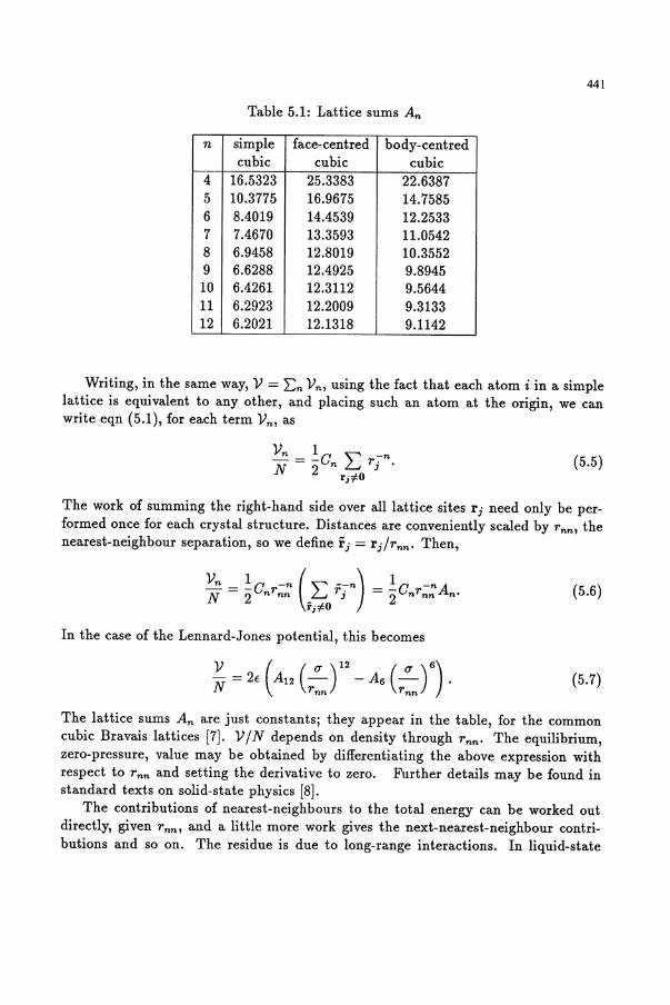
Table 5.1: Lattice sums An

n simple face-centred body-centred cubic cubic cubic

4 16.5323 25.3383 22.6387 5 10.3775 16.9675 14.7585 6 8.4019 14.4539 12.2533 7 7.4670 13.3593 11.0542 8 6.9458 12.8019 10.3552 9 6.6288 12.4925 9.8945 10 6.4261 12.3112 9.5644 11 6.2923 12.2009 9.3133 12 6.2021 12.1318 9.1142

Writing, in the same way, V = L:n Vn , using the fact that each atom i in a simple lattice is equivalent to any other, and placing such an atom at the origin, we can write eqn (5.1), for each term Vm as

(5.5)

The work of summing the right-hand side over all lattice sites rj need only be per­formed once for each crystal structure. Distances are conveniently scaled by Tnm the nearest-neighbour separation, so we define rj = rJlTnn . Then,

Vn Ie -n ('" --n) Ie -nA N = 2" nTnn _LJ Tj = 2" nTnn n'

rj;lO

(5.6)

In the case of the Lennard-Jones potential, this becomes

(5.7)

The lattice sums An are just constants; they appear in the table, for the common cubic Bravais lattices [7]. V / N depends on density through Tnn' The equilibrium, zero-pressure, value may be obtained by differentiating the above expression with respect to Tnn and setting the derivative to zero. Further details may be found in standard texts on solid-state physics [8].

The contributions of nearest-neighbours to the total energy can be worked out directly, given T nn , and a little more work gives the next-nearest-neighbour contri­butions and so on. The residue is due to long-range interactions. In liquid-state

442

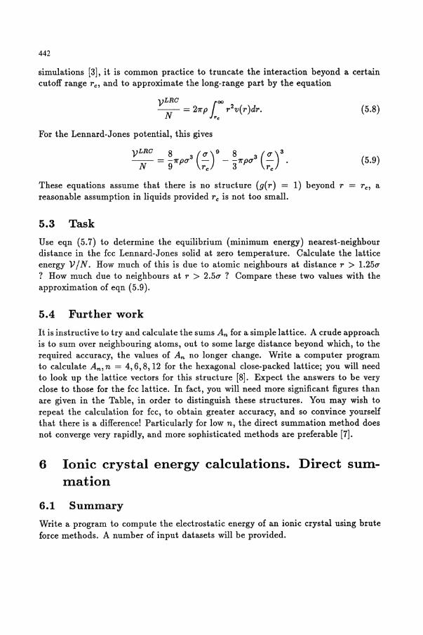
simulations [3], it is common practice to truncate the interaction beyond a certain cutoff range T e , and to approximate the long-range part by the equation

For the Lennard-Jones potential, this gives

VLRC 8 ((1')9 8 ((1')3 -- = -7rp(1'3 - - -7rp(1'3 -N 9 ~ 3 ~

These equations assume that there is no structure (g( T) = 1) beyond T reasonable assumption in liquids provided Te is not too small.

5.3 Task

(5.8)

(5.9)

Use eqn (5.7) to determine the equilibrium (minimum energy) nearest-neighbour distance in the fcc Lennard-Jones solid at zero temperature. Calculate the lattice energy V / N. How much of this is due to atomic neighbours at distance T > 1.25(1' ? How much due to neighbours at T > 2.5(1'? Compare these two values with the approximation of eqn (5.9).

5.4 Further work

It is instructive to try and calculate the sums An for a simple lattice. A crude approach is to sum over neighbouring atoms, out to some large distance beyond which, to the required accuracy, the values of An no longer change. Write a computer program to calculate An, n = 4,6,8,12 for the hexagonal close-packed lattice; you will need to look up the lattice vectors for this structure [8]. Expect the answers to be very close to those for the fcc lattice. In fact, you will need more significant figures than are given in the Table, in order to distinguish these structures. You may wish to repeat the calculation for fcc, to obtain greater accuracy, and so convince yourself that there is a difference! Particularly for low n, the direct summation method does not converge very rapidly, and more sophisticated methods are preferable [7].

6 Ionic crystal energy calculations. Direct sum­mation

6.1 Summary

Write a program to compute the electrostatic energy of an ionic crystal using brute force methods. A number of input datasets will be provided.

443

6.2 Background

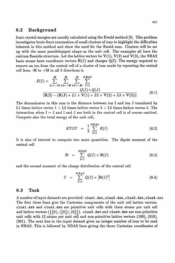
Ionic crystal energies are usually calculated using the Ewald method [9]. This problem investigates brute force summation of small clusters of ions to highlight the difficulties inherent in this method and show the need for the Ewald sum. Clusters will be set up with the same parallelepiped shape as the unit cell. The examples all have the calcium fluoride structure. Let the lattice vectors be V(l), V(2) and V(3), the NBAS basis atoms have coordinate vectors R(I) and charges Q(I). The energy required to remove an ion from the central cell of a cluster of ions made by repeating the central cell from -M to +M in all 3 directions is

M M M NBAS

E(I) = L: L: L: L: L1=-.M L2=-M L3=-M J=1

IR(J) - (R(J) + L1 x V(l) + L2 x V(2) + L3 x V(3))1 (6.1)

The denominator in this sum is the distance between ion I and ion J translated by L1 times lattice vector 1 + L2 times lattice vector 2 + L3 times lattice vector 3. The interaction when I = J and I and J are both in the central cell is of course omitted. Compute also the total energy of the unit cell,

1 NBAS

ETOT = 2 L: E(I) 1=1

(6.2)

It is also of interest to compute two more quantities. The dipole moment of the central cell

NBAS

D = L: Q(I) x R(I) (6.3) 1=1

and the second moment of the charge distribution of the central cell

NBAS

S = L: Q(I) x IR(I)21 1=1

(6.4)

6.3 Task

A number of input datasets are provided: clusi.dat, clus2. dat, clus3.dat, clus4.dat The first three lines give the Cartesian components of the unit cell lattice vectors. clus1. dat and clus2. dat are primitive unit cells with three atoms per unit cell and lattice vectors (HO), (~O~), (OH). clus3. dat and clus4. dat are non-primitive unit cells with 12 atoms per unit cell and non-primitive lattice vectors (100), (010), (001). The next line in the input dataset gives an integer number of ions to be read in NBAS. This is followed by NBAS lines giving the three Cartesian coordinates of

444

the ion position R(I) and the ion charge Q(I). Write a program to compute the electrostatic energy of a unit cell of these crystals. Compute also the individual ion energies, the unit cell dipole moment and the second moment. It is suggested that you set up clusters of ions with M = 1,3,5 and 7. Examine the results to see:-

• Does the total energy of the unit cell and the energy required to remove a single ion converge as M increases, and does the convergence depend on the central cell dipole moment and second moment?

• If the total energy and single ion energies do converge, are the results the same for the four different input datasets?

There is no need to worry about the units the result is computed in; only the relative values matter for this exercise.

7 Lennard-Jones Monte Carlo

7.1 Summary

Run a Monte Carlo program, which simulates a system of Lennard-Jones atoms. Starting from a face-centred cubic lattice, monitor the various indicators of equili­bration (potential energy, pressure, translational order parameter, mean-square dis­placement) as the crystal melts to form a liquid. Observe the effects of changing the maximum atomic displacement parameter in the Monte Carlo algorithm. Compare your results with the known properties of the Lennard-Jones fluid.

7.2 Background

A system of atoms interacting via the pairwise Lennard-Jones potential

(7.1)

is a very common test-bed for simulation programs. In this exercise, a Monte Carlo program to simulate a system of 108 Lennard-Jones atoms is provided. It can be found in the file rnclj, and it may be helpful to have a copy in front of you (on the screen or on paper) as you read this.

The program starts from an initial configuration, which can either be read in from a file or set up on a face-centred cubic (fcc) lattice. It then conducts a conventional Metropolis Monte Carlo simulation, for a predetermined number of attempted moves. The program calculates various quantities during the simulation: by monitoring these it is possible to see how quickly the system equilibrates. Following equilibration, a production run gives proper simulation averages, which can be compared with the known properties of the Lennard-Jones system, and with the output from other simulations (for example, molecular dynamics, as treated in another exercise).

445

The basic Monte Carlo method is described in the standard references [3,10,11,12]. Atoms are selected one at a time, either in sequence or randomly, for an attempted (trial) move. Each trial move involves displacing an atom by an amount (S:e,Sy,Sz) from its current position. The three Cartesian components are typically chosen, at random, from a uniform distribution between ±S7'ma"" where the maximum displace­ment parameter S7'ma", is chosen at the start of the run. The change in potential energy SV that would result from this move is then calculated, and the Metropolis prescription used to decide whether or not to accept it. Downhill moves (SV ~ 0) are accepted unconditionally; uphill moves (6V > 0) are only accepted with probability exp( -SV /kBT) where T is the temperature. For small values of S7'ma"" large atomic overlaps are unlikely to result, and the acceptance probability is high; for larger trial moves, the acceptance probability decreases. Often, D7'ma", is chosen to give an over­all acceptance rate of about 50%, but the most rapid progress through configuration space may well result from accepting a smaller proportion of larger moves. Part of this exercise is to investigate this point.

A simulation may be started from an initial configuration that is atypical of the state point of interest. It is common practice, for example, to start a series of liquid­state runs from a low-density metastable lattice configuration. The 'equilibration' of the system should then be followed carefully, before a 'production run' (giving true equili bri um averages) is undertaken.

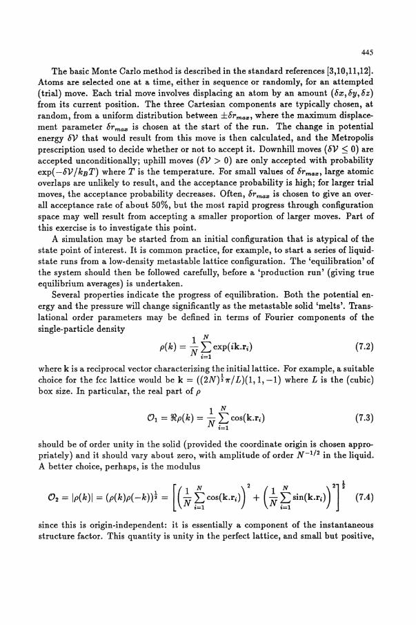
Several properties indicate the progress of equilibration. Both the potential en­ergy and the pressure will change significantly as the metastable solid 'melts'. Trans­lational order parameters may be defined in terms of Fourier components of the single-particle density

(7.2)

where k is a reciprocal vector characterizing the initial lattice. For example, a suitable choice for the fcc lattice would be k = ((2N)~7r/ L)(l, 1, -1) where L is the (cubic) box size. In particular, the real part of p

1 N 0 1 = ?Rp( k) = N?= cos(k.ri)

.=1 (7.3)

should be of order unity in the solid (provided the coordinate origin is chosen appro­priately) and it should vary about zero, with amplitude of order N- 1 / 2 in the liquid. A better choice, perhaps, is the modulus

1 [( 1 N ) 2 (1 N. ) 2] t 02=lp(k)I=(p(k)p(-k))'= Nf,;cos(k.ri) + Nf,;slll(k.ri) (7.4)

since this is origin-independent: it is essentially a component of the instantaneous structure factor. This quantity is unity in the perfect lattice, and small but positive,

446

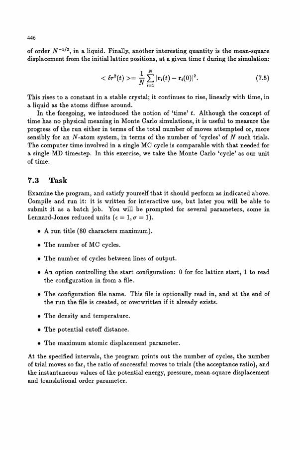
of order N- 1/ 2 , in a liquid. Finally, another interesting quantity is the mean-square displacement from the initial lattice positions, at a given time t during the simulation:

(7.5)

This rises to a constant in a stable crystal; it continues to rise, linearly with time, in a liquid as the atoms diffuse around.

In the foregoing, we introduced the notion of 'time' t. Although the concept of time has no physical meaning in Monte Carlo simulations, it is useful to measure the progress of the run either in terms of the total number of moves attempted or, more sensibly for an N-atom system, in terms of the number of 'cycles' of N such trials. The computer time involved in a single MC cycle is comparable with that needed for a single MD timestep. In this exercise, we take the Monte Carlo 'cycle' as our unit of time.

7.3 Task

Examine the program, and satisfy yourself that it should perform as indicated above. Compile and run it: it is written for interactive use, but later you will be able to submit it as a batch job. You will be prompted for several parameters, some in Lennard-Jones reduced units (E = 1, (i = 1).

• A run title (80 characters maximum).

• The number of MC cycles.

• The number of cycles between lines of output.

• An option controlling the start configuration: 0 for fcc lattice start, 1 to read the configuration in from a file.

• The configuration file name. This file is optionally read in, and at the end of the run the file is created, or overwritten if it already exists.

• The density and temperature.

• The potential cutoff distance.

• The maximum atomic displacement parameter.

At the specified intervals, the program prints out the number of cycles, the number of trial moves so far, the ratio of successful moves to trials (the acceptance ratio), and the instantaneous values of the potential energy, pressure, mean-square displacement and translational order parameter.

447

Choose a point in the liquid region of the Lennard-Jones phase diagram, and start from a lattice. Experiment with the displacement parameter 6rma." observing the effect on the acceptance ratio. Choose a value that leads to an acceptance ratio of about 50%. Then, see how long the system takes to equilibrate. This run will probably be of a few hundred cycles, perhaps more than a thousand, and it is best submitted as a batch job. Plot, as a function of the number of cycles, the four instantaneous values mentioned above. Do these various indicators of 'melting' agree with one another? Repeat the above procedure for higher and lower values of 6rma.,. What choice gives the most rapid equilibration in terms of numbers of cycles? Which represents the most efficient use of computer time? After equilibration, perform a production run, and compare the simulation averages (printed out at the end) with the known properties of the Lennard-Jones fluid. These can be obtained by running the program Ijeq. For argon, (T = 0.34nm and f = 120K. Convert your chosen density, temperature and measured pressure into S1 units: are your results sensible?

7.4 Further work

This program can be used to explore further questions of simulation efficiency, at different state points.

• The same system is investigated using molecular dynamics, in a separate exer­cise (see section 8). You may have attempted this yourself; if not, find someone who has. Compare the maximum efficiency of MC, as seen here, with that of MD, in terms of the rate of lattice melting per unit computer time.

• Perhaps the results will be dramatically different as the state point is changed. Choose two other densities and temperatures: one in the moderately dilute gas regime, and one in the solid state. What differences in behaviour do you see, as 6rma", is varied?

8 Lennard-J ones molecular dynamics

8.1 Summary

Run a molecular dynamics program, which simulates a system of Lennard-Jones atoms in three dimensions. Starting from a face-centred cubic lattice, monitor the various indicators of equilibrium (total, kinetic, and potential energy, pressure, tem­perature, translational order parameter, mean-square displacement) as the crystal melts to form a liquid. Explore the effect of changing the initial temperature. Plot your results as a function of time, and compare with the known properties of the Lennard-Jones fluid.

448

8.2 Background

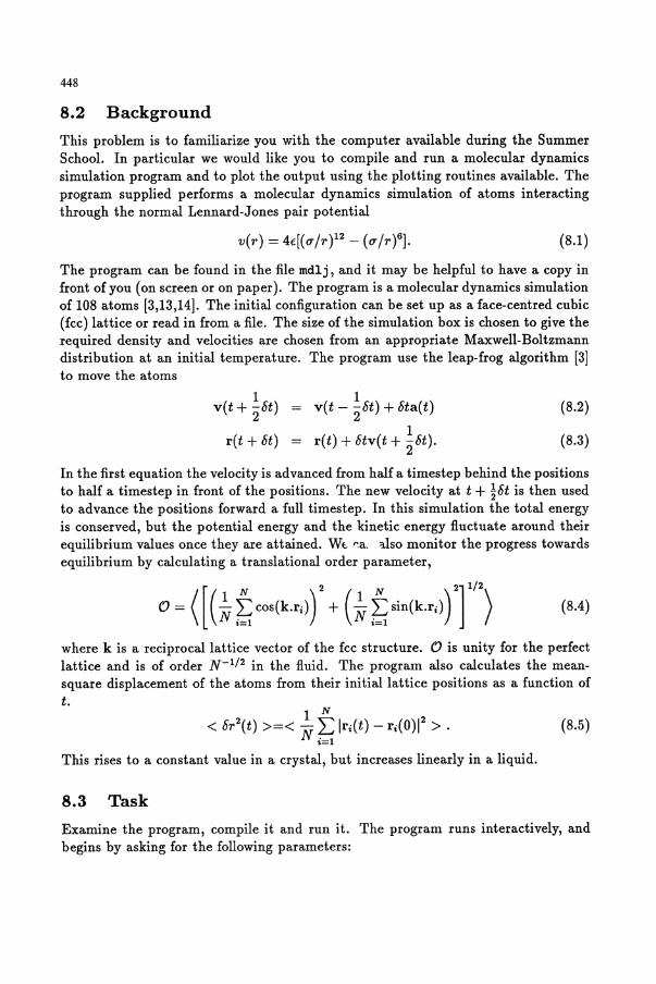
This problem is to familiarize you with the computer available during the Summer School. In particular we would like you to compile and run a molecular dynamics simulation program and to plot the output using the plotting routines available. The program supplied performs a molecular dynamics simulation of atoms interacting through the normal Lennard-Jones pair potential

(8.1)

The program can be found in the file mdlj, and it may be helpful to have a copy in front of you (on screen or on paper). The program is a molecular dynamics simulation of 108 atoms [3,13,14]. The initial configuration can be set up as a face-centred cubic (fcc) lattice or read in from a file. The size of the simulation box is chosen to give the required density and velocities are chosen from an appropriate Maxwell-Boltzmann distribution at an initial temperature. The program use the leap-frog algorithm [3] to move the atoms

1 v(t+ 2"0t)

r( t + ot)

1 v(t - 2"0t) + ota(t)

1 r(t) + otv(t + 2"0t).

(8.2)

(8.3)

In the first equation the velocity is advanced from half a timestep behind the positions to half a timestep in front of the positions. The new velocity at t + tot is then used to advance the positions forward a full timestep. In this simulation the total energy is conserved, but the potential energy and the kinetic energy fluctuate around their equilibrium values once they are attained. Wt- <:a. 'l.lso monitor the progress towards equilibrium by calculating a translational order parameter,

(8.4)

where k is a reciprocal lattice vector of the fcc structure. 0 is unity for the perfect lattice and is of order N- 1 / 2 in the fluid. The program also calculates the mean­square displacement of the atoms from their initial lattice positions as a function of t.

1 N < or2(t) >=< N L Iri(t) - ri(0)1 2 > .

i=l

(8.5)

This rises to a constant value in a crystal, but increases linearly in a liquid.

8.3 Task

Examine the program, compile it and run it. The program runs interactively, and begins by asking for the following parameters:

449

• a title of not more than eighty characters;

• the number of steps (say 1000);

• the number of steps between output lines (say 10);

• a flag to determine whether the configuration is from a lattice or file, 0 for a lattice start, 1 for a file start;

• the name of a file for the output configuration, not more than 30 characters;

• the reduced density (p0-3);

• the reduced starting temperature (kT / e);

• the reduced cut-off distance for the Lennard-Jones potential (say 2.50-);

• the reduced timestep (say 0.005).

The routine then converts LJ units to simulation units which are based on a box length of one. The long-range corrections appropriate to the potential and virial are calculated, and a reciprocal lattice vector of the starting lattice is calculated. The accumulators for the properties and their fluctuations are set to zero. The program then begins the main loop over time steps. In this loop the atoms are moved using the second leapfrog equation, the forces and accelerations at the new positions are calculated and the velocities are advanced using the first leapfrog equation. The order parameter and the temperature are calculated. Finally the accumulators are incremented with information from the current time step. When the main loop is completed, final averages are computed and displayed. There are eight subroutines:

• SUBROUTINE FCC sets up an initial configuration in an fcc lattice;

• SUBROUTINE COMVEL chooses the initial velocities at a particular temperature;

• SUBROUTINE READCN reads in a starting configuration;

• SUBROUTINE FORCE calculates the forces, accelerations, energy, and virial;

• SUBROUTINE MOVE advances the velocities and positions of all the atoms;

• SUBROUTINE KINET calculates the kinetic energy;

• SUBROUTINE ORDER calculates the translational order parameter, which is one for a perfect fcc lattice and close to zero for a liquid;

• SUBROUTINE WRITCN writes out a configuration to file.

450

In [15) you will find a phase diagram of the three-dimensional Lennard-Jones fluid. Try to simulate at a point in the liquid region i.e. where the translational order parameter is close to zero. Remember that if you start from an expanded lattice, the potential energy will rise as the lattice melts and the temperature (kinetic energy) will fall. Be careful that it does not fall so far from your starting temperature that your simulation freezes. Plot the following as a function of time:

• the total energy, corrected for the cut-off (CUTENERGY);

• the kinetic energy (KINETIC);

• the potential energy (POTENT);

• the pressure (PRESSURE);

• the temperature (TEMPER);

• the order parameter (OPARAM);

• the mean-square dispalcement (MDISP).

Repeat these plots starting from a disordered configuration prepared at the temper­ature you require. Make sure that you are completely familiar with compiling and running FORTRAN programs, using the editor to manipulate data and plotting the data. You will find a parameterized equation of state for the Lennard-Jones fluid on the computer. This equation was fitted to a large amount of previous simulation data [16). The equation is accessed by running the job ljeq. You feed in the reduced temperature and density and it returns an estimate of the thermodynamic properties. Compare these results to your average values for the density and final temperature of your run.

8.4 Further work

• Experiment with the time-step, and the length of the simulation run.

• The same system is investigated using Monte Carlo in section 7. You may have attempted this yourself; if not, find someone who has. Compare the efficiency of molecular dynamics and Monte Carlo in terms of the rate of lattice melting per unit computer time.

• Run the simulation for state points typical of a dilute gas and a crystal. Plot the mean square displacement as a function of time in each case.

451

9 Monte Carlo by hand

9.1 Summary

In this exercise you will try some simple Monte Carlo simulations by hand, using a six-sided die to generate random numbers. The idea is to study a small, one­dimensional, Ising spin system, employing both asymmetric and symmetric transition probabilities, to get a feel for the way the method works. This leads on, in a later project, to computer simulations of the same system.

9.2 Background

The Ising model is one of the most fundamental models in statistical physics. At each site of a lattice is a spin Si which may point up or down: Si = ±1. There are interactions of the form

Eij = -J SiSj (9.1) between nearest-neighbour spins i and j, where J (here assumed positive) is a coupling constant. This system can be thought of as a representing a ferromagnetic metal. We can add an external magnetic field (a term of the form Ei = H Si) if we wish, but here we consider the field-free case for simplicity. An isomorphism with the lattice gas model (each site either occupied or unoccupied) means that the system can also represent, in a highly idealized way, an atomic liquid or gas. The phase transitions in these types of model reflect those of real systems, thanks to universality, although for the simple one-dimensional system studied here there is no phase transition.

In this exercise we use small Ising systems to test out the basic simulation meth­ods. Useful background material on the simulation of spin systems can be found in the standard references [10,11,17]. The basic Monte Carlo method consists of repetitions of the following steps:

• select a spin (sequentially or at random);

• calculate a transition probability for flipping this spin;

• choose to flip the spin or not, according to this probability.

There are many different ways of choosing the transition probabilities, and we inves­tigate two here.

For this task you require pen and paper, and a six-sided die (provided). Consider a one-dimensional system of 8 Ising spins, as shown in Figure 9.1. Each spin has two nearest neighbours, with interaction energies given by eqn (9.1). As usual, periodic boundary conditions apply.

Consider flipping a spin. This will, in general, result in an energy change !lE. The Metropolis formula [18] for the probability of accepting this flip is

P(!lE) = min(l,exp( -!lE/kT)) (9.2)

452

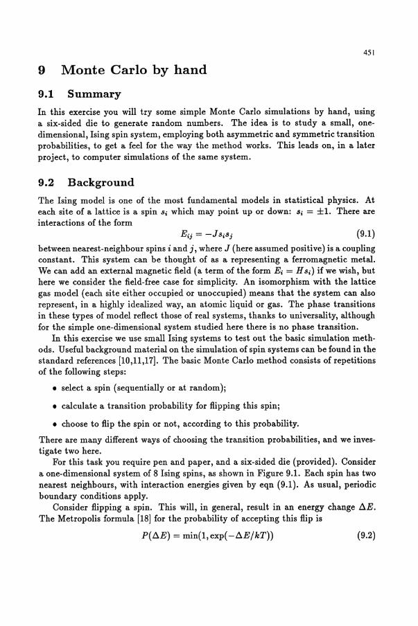
Figure 9.1: A one-dimensional configuration of spins with periodic boundary condi­tions

(8) 1 2 3 4 5 6 7 8 (1)

I 1 tll1tltll1tl111 t I

F' 92 A I H!:ure . : ow-energy one-d' 1 fi f ImenSlOna con 19ura IOn 0 spIns

(8) 1 2 3 4 5 6 7 8 (1)

f t tltltltltltltlt 1 1

where T is the temperature and k Boltzmann's constant. In other words, if 6..E is negative (downhill), accept the flip unconditionally; if 6..E is positive (uphill), accept with probability exp( -6..E/kT). An alternative, the Glauber formula [19] is more symmetrical with respect to uphill and downhill moves:

P(6..E) = exp( -6..E/kT) 1 + exp( -6..E/kT)

(9.3)

Both these prescriptions satisfy the basic equation of detailed balance (or microscopic reversibility), i. e. that P(6..E)/ P( -6..E) = exp( -6..E /kT). This ensures that the simulation, in principle, generates proper canonical ensemble averages. (Here we are assuming equal underlying probabilities for attempting a forward move and the reverse move.) Accepting a flip 'with a given probability' is simply a matter of choosing a random number uniformly from a given range, typically (0,1). Suppose we wish to accept a flip with probability 30%; if the random number is 0.3 or less, we flip the spin, if it is more than 0.3 we do not. In special cases, when only a small set of acceptance probabilities are possible, the decision can be made by tossing a coin or throwing a die.

9.3 Task

Consider the one-dimensional system of Figure 9.1, with a temperature chosen such that J/kT = ~ln2. What are the possible changes 6..E/kT involved in flipping a spin in this system? Calculate the flip probabilities for all possible arrangements of neighbouring spins, for each ofthe two prescriptions above, eqns (9.2),(9.3). For these probabilities, it should be easy to carry out a Monte Carlo simulation of the system,

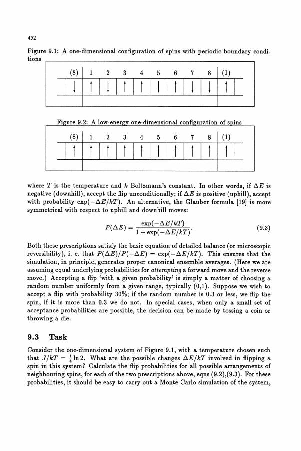
453

Fi ure 9.3: A hi

using a six-sided die as a random number generator. Starting from the configuration of Figure 9.1, carry out a few sweeps (one sweep is one attempted Monte Carlo flip per spin, i. e. 8 flips here), using each prescription. For simplicity, select each spin for flipping sequentially. Keep a record of the flip probabilities, whether or not you need to throw the die, and the outcome, for each attempt. Try to get a feel for the relative rate at which flips actually occur: which algorithm moves the system through configuration space the fastest?

Consider what would happen to an initial configuration with the lowest possible energy, and to one with the highest possible energy, as shown in Figures 9.2, 9.3, under these algorithms. What is the evolution likely to be at very high temperatures and at very low temperatures?

10 Hard sphere Monte Carlo in one dimension

10.1 Summary

Write a Monte Carlo program for a one dimensional system of hard spheres. Using a modest number of particles (e.g. N = 50), and choosing some suitable density, run the program for a few thousand Monte Carlo cycles and calculate the pressure. Compare with the exact result in the thermodynamic limit (N --t 00).

10.2 Background

Simulation studies of model liquids such as hard spheres in three dimensions and hard disks in two dimensions have played a key role in understanding the structure of simple liquids and in the development of theories of liquids [15]. In this exercise you are going to write a Monte Carlo program for hard disks whose centres are confined to a line.

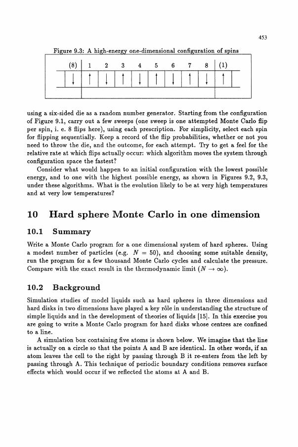
A simulation box containing five atoms is shown below. We imagine that the line is actually on a circle so that the points A and B are identical. In other words, if an atom leaves the cell to the right by passing through B it re-enters from the left by passing through A. This technique of periodic boundary conditions removes surface effects which would occur if we reflected the atoms at A and B.

454

Figure 10.1: A one-dimensional system of N = 5 hard spheres in periodic boundaries (with two periodic ima es shown

L

The properties of our one dimensional fluid depend only on the density or packing fraction of atoms on the line. This packing fraction, Tf, is an input variable to the program

Tf = NulL (10.1 )

where N is the number of atoms on the line, 0' is the diameter of each atom and L is the length of the line. A Monte Carlo move is made by choosing an atom at random or in order and giving it a small random displacement to the left or to the right. If the atom does not overlap with one of its neighbours, the move is accepted. If the atom overlaps the move is rejected and the old configuration is counted as the next step in the chain. This recipe generates a Markov chain whose limiting distribution is proportional to the Boltzmann factor of the fluid. Unweighted averages calculated over the states in the chain are equivalent to averages in the canonical ensemble. It is possible to calculate the radial distribution function and hence the pressure of the hard sphere fluid. The maximum possible displacement of an atom is adjusted so that about 50% of the trial moves are accepted. The radial distribution is calculated in the simulation by sorting all pair separations into a histogram [3]. Suppose we sort every tenth cycle, so that there are a total of Trun sorts, and that a particular bin of the histogram, corresponding to the interval (r,r + 8r), contains nhi.(b) pairs. Then the average number of atoms whose distance from a given atom in the fluid lies in this interval, is

(10.2)

The average number of atoms in same interval for the ideal gas at the same density is

(10.3)

The radial distribution function is

1 g(r + 28r) = n(b)lnid(b). (10.4)

455

The compression factor of the fluid can be calculated from the simulation by extrap­olating g( 1') to contact,

(10.5)

This can be compared to the exact result which can be derived in the thermodynamic limit by factorizing the configurational partition function [20]

PL/NkBT = 1/(1- 'f/). (10.6)

10.3 Task

You begin by choosing a reasonable value of N and of 'f/. We recommend you simulate about 50 atoms at a packing fraction of say 0.60. It is convenient to use a line of unit length and to calculate the appropriate value of (J'. The program can be divided into a number of stages.

10.3.1 Input

We begin by setting up the atom positions. You should allow for two choices:

• Setting the 50 atoms at equal intervals on the line, with atom 1 at the origin;

• Reading a random, or aged configuration from the file mc1ddat.

The program should now ask you for a number of parameters:

• A run title (say 'test run one');

• The number of Me cycles (say 10000);

• The number of steps between output (say 100);

• The density (say 0.6);

• The interval for calculating g(1') (say DELR = 0.02);

• The name of the input file for the configuration, which is also used for dumping the final configuration (say mC1ddat);

• A flag which tells the program whether you want to run from a disordered start or a lattice start (say 0 or 1).

You will need to use a random number generator, which you can start by calling the NAG library subroutine G05CBF(O.O). The argument of this routine changes the seed of the random number generator.

456

10.3.2 Setup

• It is useful at this stage to zero the accumulator or histogram you will use to calculate the radial distribution function i.e. set IRDF(I)=O for I=1, NRDF (NRDF=100 ).

• You will need to choose a maximum displacement for the particles, say MAXDIS = SIGMA/20. o.

• You should convert the interval for the RDF calculation to units with L = 1 i.e. set DELR = DELR * SIGMA.

• Calculate the maximum distance for sorting for the RDF, i.e. set RDFMAX

DELR * REAL(NRDF).

• Zero any other accumulators you may need.

10.3.3 Loop over cycles

In each cycle you will loop over all atoms, in order. You should try to move each atom one at a time.

RXINEW = RX(I) + (2.0 * G05CAF( DUMMY )-1.0) * MAXDIS

This generates a uniform random displacement between -MAXDIS and +MAXDIS. If MAXDIS is less than SIGMA, then the particle in the new position may overlap with its neighbours. We only need to check the neighbours to the left and right of the atom we have just moved. In checking for overlap make sure you apply the minimum image convention for the atom separation

RXIJ = RXIJ - ANINT( RXIJ )

and be careful when comparing distances that you only consider the magnitude not the sign of the interatomic separation. Remember overlaps occur if RXIJ<SIGMA. If an overlap occurs go back to the old configuration and use the old configuration as the next step in the chain.

10.3.4 Periodic operations

There are a number of operations which can be carried out periodically.

• Adjust the maximum displacement MAXDIS every ten cycles so that approxi­mately half the configurations are accepted (optional).

• Output the following information every ten cycles:

- the number of cycles;

457

- the number of moves accepted;

- the acceptance ratio;

- the maximum displacement.

• Write the current configuration to the restart file, mclddat, every 500 cycles (optional).

• Calculate the radial distribution function every twenty cycles. This procedure involves looping over all distinct pairs of atoms and calculating the centre of mass separation using the minimum image convention. These separations are sorted into a histogram IRDF where the bins are of thickness DELR. The radial distribution function g( r) is calculated from

GR(IR) = IRDF(IR)/REAL(N)/ACRDF/(DELR*DENS*2.0)

where ACRDF is the number of sorts, DENS is N / L for L = 1, and the factor of 2 takes care of the fact that we are sorting atoms to the left and right of a given atom.

At the end of the simulation g( r) as a function of r / (j should be tabulated and stored. The appropriate r / (j corresponds to the middle of the histogram bin [3]. At the end ofthe calculation you should plot g( r) against r / (j • The compression factor of the fluid should be calculated.

10.4 Further work

• How is the compression factor affected by the length of the run?

• How is the compression factor affected by the histogram interval?

• How is the compression factor affected by using different seeds for the random number generator?

• How is the compression factor affected by changing the system size?

• How does the initial configuration affect the convergence of the run?

• Is the compression factor obtained from this program more or less accurate than the value obtained from the corresponding dynamic simulation (see section 11) ?

458

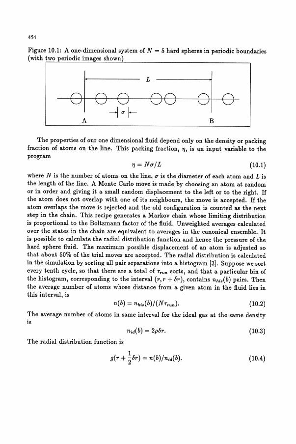
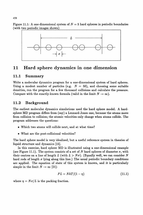
Figure 11.1: A one-dimensional system of N = 5 hard spheres in periodic boundaries (with two periodic images shown

L

11 Hard sphere dynamics in one dimension

11.1 Summary

Write a molecular dynamics program for a one-dimensional system of hard spheres. Using a modest number of particles (e.g. N = 50), and choosing some suitable densities, run the program for a few thousand collisions and calculate the pressure. Compare with the exactly-known formula (valid in the limit N ~ 00).

11.2 Background

The earliest molecular dynamics simulations used the hard sphere model. A hard­sphere MD program differs from (say) a Lennard-Jones one, because the atoms move from collision to collision; the atomic velocities only change when atoms collide. The program addresses the questions:

• Which two atoms will collide next, and at what time?

• What are the post-collisional velocities?

The hard sphere model is very idealized, but a useful reference system in theories of liquid structure and dynamics [15].

In this exercise, hard sphere MD is illustrated using a one-dimensional example (see Figure 11.1). The system consists of a set of N hard spheres of diameter u, with their centres on a line oflength L (with L > Nu). (Equally well, we can consider N hard rods of length u lying along this line.) The usual periodic boundary conditions are applied. The equation of state of this system is known, and it is particularly simple in the limit N ~ 00 [21]:

PL = NkT/(l-1]) (11.1)

where 1] = N u / L is the packing fraction.

459

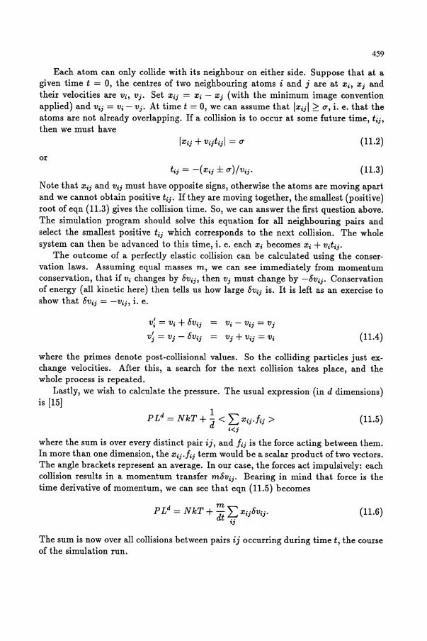
Each atom can only collide with its neighbour on either side. Suppose that at a given time t = 0, the centres of two neighbouring atoms i and j are at Xi, Xi and their velocities are Vi, Vi. Set xii = xi - Xi (with the minimum image convention applied) and Vii = vi - Vi. At time t = 0, we can assume that IXiil 2:: u, i. e. that the atoms are not already overlapping. If a collision is to occur at some future time, tij, then we must have

(11.2)

or (11.3)

Note that Xii and Vii must have opposite signs, otherwise the atoms are moving apart and we cannot obtain positive tij. If they are moving together, the smallest (positive) root of eqn (11.3) gives the collision time. So, we can answer the first question above. The simulation program should solve this equation for all neighbouring pairs and select the smallest positive t ij which corresponds to the next collision. The whole system can then be advanced to this time, i. e. each Xi becomes Xi + Vitij.

The outcome of a perfectly elastic collision can be calculated using the conser­vation laws. Assuming equal masses m, we can see immediately from momentum conservation, that if Vi changes by 5Vij, then Vj must change by -5Vij. Conservation of energy (all kinetic here) then tells us how large 5Vij is. It is left as an exercise to show that 5Vij = -Vij, i. e.

V~ = Vi + 5Vij

vj = Vj - 5Vij

Vi - Vij = Vj

Vj + Vii = vi (11.4)

where the primes denote post-collisional values. So the colliding particles just ex­change velocities. After this, a search for the next collision takes place, and the whole process is repeated.

Lastly, we wish to calculate the pressure. The usual expression (in d dimensions) is [15]

d 1" P L = NkT + d < !--<. Xij·lij >

• 3

(11.5)

where the sum is over every distinct pair ij, and lij is the force acting between them. In more than one dimension, the xij.lij term would be a scalar product oftwo vectors. The angle brackets represent an average. In our case, the forces act impulsively: each collision results in a momentum transfer m5Vij. Bearing in mind that force is the time derivative of momentum, we can see that eqn (11.5) becomes

(11.6)

The sum is now over all collisions between pairs ij occurring during time t, the course of the simulation run.

460

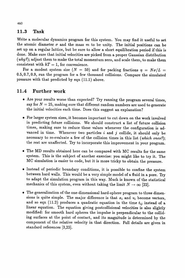
11.3 Task

Write a molecular dynamics program for this system. You may find it useful to set the atomic diameter (J" and the mass m to be unity. The initial positions can be set up on a regular lattice, but be sure to allow a short equilibration period if this is done. Make sure that initial velocities are picked from a proper Gaussian distribution (why?); adjust them to make the total momentum zero, and scale them, to make them consistent with kT = 1, for convenience.

For a modest system size (N = 50) and for packing fractions 'f/ = N (J" / L = 0.5, 0.7,0.9, run the program for a few thousand collisions. Compare the simulated pressure with that predicted by eqn (11.1) above.

11.4 Further work

• Are your results worse than expected? Try running the program several times, say for N = 25, making sure that different random numbers are used to generate the initial velocities each time. Does this suggest an explanation?

• For larger system sizes, it becomes important to cut down on the work involved in predicting future collisions. We should construct a list of future collision times, making sure to reduce these values whenever the configuration is ad­vanced in time. Whenever two particles i and j collide, it should only be necessary to re-evaluate a few of the collision times in this list (which ones?); the rest are unaffected. Try to incorporate this improvement in your program.

• The MD results obtained here can be compared with MC results for the same system. This is the subject of another exercise: you might like to try it. The MC simulation is easier to code, but it is more tricky to obtain the pressure.

• Instead of periodic boundary conditions, it is possible to confine the system between hard walls. This would be a very simple model of a fluid in a pore. Try to adapt the simulation program in this way. Much is known of the statistical mechanics of this system, even without taking the limit N --+ 00 [22].

• The generalization of the one-dimensional hard-sphere program to three dimen­sions is quite simple. The major difference is that Xi and Vi become vectors, and so eqn (11.2) produces a quadratic equation in the time tij instead of a linear equation. The equation giving postcollisional velocities is also slightly modified: for smooth hard spheres the impulse is perpendicular to the collid­ing surfaces at the point of contact, and its magnitude is determined by the component of the relative velocity in that direction. Full details are given in standard references [3,23].

461

12 A Monte Carlo simulation of Lennard-Jones atoms in one dimension

12.1 Summary

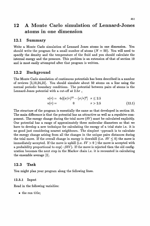
Write a Monte Carlo simulation of Lennard Jones atoms in one dimension. You should write the program for a small number of atoms (N = 50). You will need to specify the density and the temperature of the fluid and you should calculate the internal energy and the pressure. This problem is an extension of that of section 10 and is most easily attempted after that program is written.

12.2 Background

The Monte Carlo simulation of continuous potentials has been described in a number of reviews [3,10,24,25]. You should simulate about 50 atoms on a line using the normal periodic boundary conditions. The potential between pairs of atoms is the Lennard-Jones potential with a cut-off at 2.50' ,

v(r) = 4€[(0'/r)12 - (0'/r)6] r:::; 2.5

v(r) = 0 r>2.5 (12.1 )

The structure of the program is essentially the same as that developed in section 10. The main difference is that the potential has an attractive as well as a repulsive com­ponent. The energy change during the trial move (8V) must be calculated explicitly. Our potential has a range of approximately three molecular diameters so that we have to develop a new technique for calculating the energy of a trial state i.e. it is no good just considering nearest neighbours. The simplest ."pproach is to calculate the energy change arising from all the changes in the unique pairs distances during the trial move. If the overall change in energy is downhill (i.e. 8V :::; 0) the move is immediately accepted. If the move is uphill (i.e. 8V > 0 ) the move is accepted with a probability proportional to exp( -,88V). If the move is rejected then the old config­uration becomes the next step in the Markov chain i.e. it is recounted in calculating the ensemble average [3].

12.3 Task

You might plan your program along the following lines.

12.3.1 Input

Read in the following variables:

• the run title;

462

• the number of cycles;

• the number of cycles between output lines;

• the number of steps between saving the configuration;

• the interval for updating the maximum displacement;

• the name of the file for dumping configurations;

• a flag to decide if you want a lattice start or a start from a file;

and the following in the usual reduced Lennard-Jones units:

• the density;

• the cutoff;

• the temperature.

The initial positions of the atoms on the lattice can now be set-up by reading them from the configuration file or placing the atoms on a lattice at equal intervals along the line.

12.3.2 Setup

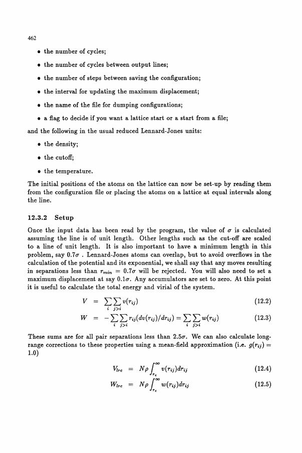
Once the input data has been read by the program, the value of 0" is calculated assuming the line is of unit length. Other lengths such as the cut-off are scaled to a line of unit length. It is also important to have a minimum length in this problem, say 0.70" . Lennard-Jones atoms can overlap, but to avoid overflows in the calculation of the potential and its exponential, we shall say that any moves resulting in separations less than 1'min = 0.70" will be rejected. You will also need to set a maximum displacement at say 0.10". Any accumulators are set to zero. At this point it is useful to calculate the total energy and virial of the system.

v (12.2) i i>i

w (12.3) i i>i i>i

These sums are for all pair separations less than 2.50". We can also calculate long­range corrections to these properties using a mean-field approximation (i.e. 9(1'ii) = 1.0)

Vlrc = N plOO v(1'ii)d1'ii rc

mrc = N p 100 w( 1'ii )d1'ii rc

(12.4)

(12.5)

The virial is related to the pressure of the one-dimensional fluid

12.3.3 Main loop

p _ NkBT < W> - L + L

463

(12.6)

The program now loops over cycles. Inside this loop we loop over all atoms on the line in order. Each atom is given a uniform random displacement left or right using a random number generator. If the move results in a significant overlap i.e. any Tij < Tmin, it is immediately rejected and the old configuration is recounted as the next step in the chain. If the move is not rejected on these grounds, the change in energy and virial for the move is calculated. Note that the long-range corrections are constant during these moves. If the change in energy is downhill (i.e. negative), the move is accepted and the total energy and virial of the line are updated. If the move is uphill (i.e. 6V > 0 where 6V = Vnew - Void), we calculate exp( -(36V) where (3 = l/kB T. We compare exp( -(36V) with a uniform random number in the range zero to one. If the exponential is greater than the random number we accept the move, if it is less we reject the move and recount the old configuration as the next step in the chain. This sequence of events requires some careful programming.

12.3.4 Periodic operations

In the main loop it is necessary to perform a number of periodic operations. The maximum displacement should be adjusted so that approximately half the attempted moves are accepted. Output, such as the number of cycles, the number of accepted moves, the energy and virial (including their long-range corrections), and the value of the maximum displacement should be written to the screen or to a file for inspection. The current configuration should be dumped to the configuration file to allow for a restart.

12.3.5 Winding up

At the end of the main loop you should use the accumulators to calculate the av­erage configurational energy and pressure and the fluctuation in these properties. Throughout the simulation you have been incrementing the energy and virial of your initial configuration each time you accept an atom move. At this point you could recalculate the energy and virial of the complete line, using a sum over all pairs. This should agree with the value that you are carrying for the energy and virial to within the machine accuracy. It is a useful check that you are calculating all the interactions and the energy changes properly. In this exercise, we would like you to construct the program, and run it for a number of densities and temperatures, establishing the trends in the energy and pressure for your one dimensional fluid.

464

12.4 Further work

• Plot the internal energy of the fluid as a function of temperature for a number of fixed densities. Calculate the specific heat at constant volume by graphically differentiating the energy with respect to temperature. Plot Cv against T. Does this system exhibit a solid-liquid or a liquid-gas phase transition? You could also calculate Cv using the appropriate fluctuation formula in the canonical ensemble.

• You should consider how your results depend on the length of the run, and the seed of the random number generator.

• You can start the simulation from a lattice configuration or from a disordered configuration which you create at the end of your first run and update with subsequent runs. How does the starting configuration affect the convergence of the Markov chain? Is a 50% acceptance ratio for the trial moves the optimum value? How does the optimum acceptance ratio compare with the value you found in the Monte Carlo simulation of the hard spheres on a line (section 10)?

• This program is easily extended to three dimensions. How does the definition of the pressure depend on the dimensionality? How will the two long-range corrections change? If you rewrite the program for three dimensions you could compare your results for the energy and pressure with those from section 7.

13 Ising model simulations

13.1 Summary

This project involves using the Ising model to test various simulation techniques. The aim is to compare Monte Carlo, employing both asymmetric and symmetric transition probabilities, with a simple deterministic cellular automaton algorithm. There is the possibility also to look into multispin coding techniques for vector and parallel computers. This project would be suitable for an individual, or for a team, each individual pursuing a different aspect.

13.2 Background

The Ising model is described in a separate exercise (see section 9) but for completeness we give the details again here. The Ising model is one of the most fundamental models in statistical physics. At each site of a lattice is a spin Si which may point up or down: Si = ± 1. There are interactions of the form

(13.1 )

465

between nearest-neighbour spins i and j, where J (here assumed positive) is a coupling constant. This system can be thought of as a representing a ferromagnetic metal. We can add an external magnetic field (a term of the form Ei = H Si) if we wish, but here we consider the field-free case for simplicity. An isomorphism with the lattice gas model (each site either occupied or unoccupied) means that the system can also represent, in a highly idealized way, an atomic liquid or gas. The phase transitions in these types of model reflect those of real systems, thanks to universality.

The statistical mechanics of the one-dimensional Ising model, i. e. a chain of spins, can be worked out quite easily. There are no phase transitions, but it is a useful simulation 'test bed'. The two-dimensional Ising model, for infinite system size in zero field is also an exactly-solved problem. Here, there is a first-order phase transition between ordered and disordered states, below a critical temperature. Further details may be found in standard texts on statistical mechanics (for example [26]). So the simulated properties (for large enough systems) can be compared with known ones. Another approach is to study a system small enough that the statistical properties can be obtained by direct counting of states.

In this project we use small Ising systems to test out basic simulation methods. Useful background material on the simulation of spin systems can be found in the standard references [10,11,17). The basic Monte Carlo method consists of repetitions of the following steps:

• select a spin (sequentially or at random);

• calculate a transition probability for flipping this spin;

• choose to flip the spin or not, according to this probability.

In the effort to find faster and faster algorithms, much interest has centred in recent years on the relative efficiencies of different ways of choosing the transition probabili­ties, on ways of coding the program so as to consider many spins at once, and on the rapid generation of good random number sequences. There have also been some inves­tigations of deterministic methods (cellular automata) of generating configurations, which do not involve random numbers at all. By tricks such as these, impressive per­formance can be squeezed out of even small microcomputers, and truly awesome flip rates achieved on supercomputers. The above references provide excellent accounts of these developments.

In fact, most of the underlying ideas have been around for many years. The present project is very much in the spirit of the work of Friedberg and Cameron [27) who took a small Ising lattice, and used it to test the performance of their simulation program. Their paper describes the basic Monte Carlo method, covering many technical points such as the selection of spins for flipping, the division of the system into two independent sublattices, the basic multi spin coding approach, the choice between different transition probabilities, the danger of being locked into a region of configuration space, and the analysis of the results for statistical errors. Some of these points will be treated below.

466

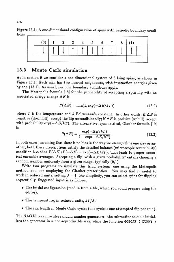
Figure 13.1: A one-dimensional configuration of spins with periodic boundary condi­tions

(8) 1 2 3 4 5 6 7 8 (1)

I 1 tilltltilltllil t I

13.3 Monte Carlo simulation

As in section 9 we consider a one-dimensional system of 8 Ising spins, as shown in Figure 13.1. Each spin has two nearest neighbours, with interaction energies given by eqn (13.1). As usual, periodic boundary conditions apply.

The Metropolis formula [18J for the probability of accepting a spin flip with an associated energy change I:l.E is

P(I:l.E) = min(l,exp( -I:l.E/kT)) (13.2)

where T is the temperature and k Boltzmann's constant. In other words, if I:l.E is negative (downhill), accept the flip unconditionally; if I:l.E is positive (uphill), accept with probability exp( -I:l.E/kT). The alternative, symmetrical, Glauber formula [19J IS

P(I:l.E) = exp( -I:l.E/kT) 1 + exp( -I:l.E/kT)

(13.3)

In both cases, assuming that there is no bias in the way we attempt flips one way or an­other, both these prescriptions satisfy the detailed balance (microscopic reversibility) condition i. e. that P(I:l.E)/P(-I:l.E) = exp(-I:l.E/kT). This leads to proper canon­ical ensemble averages. Accepting a flip 'with a given probability' entails choosing a random number uniformly from a given range, typically (0,1).

Write two programs to simulate this Ising system: one using the Metropolis method and one employing the Glauber prescription. You may find it useful to work in reduced units, setting J = 1. For simplicity, you can select spins for flipping sequentially. Suggested input is as follows.

• The initial configuration (read in from a file, which you could prepare using the editor ).

• The temperature, in reduced units, kT/J.

• The run length in Monte Carlo cycles (one cycle is one attempted flip per spin).

The NAG library provides random number generators: the subroutine G05CCF initial­izes the generator in a non-reproducible way, while the function G05CAF ( DUMMY )

467

returns a random number in the range (0,1). Both G05CAF and its dummy argument DUMMY should be declared DOUBLE PRECISION. Suggested output at user-specified in­tervals:

• The total energy.

• The magnetization (i.e. number of up spins minus number of down spins).

• The ratio of flips accepted to flips attempted.

You might also like to print snapshots of the configurations. These programs will probably be fast enough to run interactively.

Run the programs (with your choice of temperature) to see what happens, to an initial configuration with the lowest possible energy, and to one with the highest possible energy, as shown in Figures 9.2, 9.3, under these two algorithms. What happens at very high temperatures and at very low temperatures?

13.4 Multispin coding

This simple one-dimensional system can also be used to illustrate the ideas behind multi spin coding and the running of Monte Carlo simulations on parallel computers. We have been selecting spins sequentially for flipping; random selection is another way of going about things. Yet a third possibility is to look first at all the odd­numbered spins, flip them with the appropriate probabilities, and then consider all the even-numbered spins in a similar way. Because the interactions are restricted to nearest neighbours, it does not matter in what order we consider spins within each of these two sets: the calculations involved in flipping spins 1, 3, 5, and 7, for example, are independent of one another. These four spins could equally well be treated in parallel, and updated all at once. Then, attention could be focused on spins 2, 4, 6, 8, and so on. Try this updating scheme in your program, for the initial configurations discussed above. You should be able to see some potential pitfalls of this method in special cases, but for non-pathological starting conditions it should be just as valid as the other methods. In two (and also three) dimensions, it is possible to adopt a black-white checkerboard identification of two independent sublattices. This is the approach used by Friedberg and Cameron [27] and it has been described several times since (see e. g. Chapter 10 of ref. [10] and references therein).

13.5 Cellular automaton method

A cellular automaton (CA) uses completely deterministic rules for updating a config­uration of (in this case) spins. For the Ising model on a lattice in zero applied field, as long as there are an even number of neighbours for each site, there is a simple rule that allows the system to evolve while conserving the energy. Consequently, this sim­ulation probes the micro canonical rather than the canonical ensemble. Nonetheless,

468

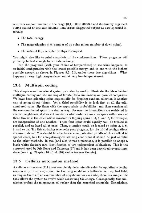
Fi ure 13.2: Cellular automaton simulation

this is a potentially useful route to statistical mechanical properties. The motivation for introducing it is that, for such a simple model, the generation of the random numbers in conventional Monte Carlo can be the most time-consuming operation. A cellular automaton requires no random numbers, except to set up an initial config­uration. This approach has been employed by Herrmann [28], and the original CA model is due to Pomeau and Vichniac [29,30]. The method is valid in any number of dimensions; here we take the one-dimensional example as a simple illustration.

The CA rule is based on the division into two sublattices, mentioned above, and the observation that if a spin is surrounded by equal numbers of up and down spins, then flipping it does not change the energy. The rule is simply that all such spins on a given sublattice should be flipped simultaneously. Then, the same procedure is applied to the other sublattice. This prescription is repeated many times in the course of a simulation. Consider the starting configuration of Figure 13.1, which is given again at the top of Figure 13.2. We apply the rule to the 'odd-numbered' sublattice first. Of these spins, only numbers 3 and 7 have one up and one down neighbour, so only these are flipped. This gives the second configuration in the Figure. Now we apply the rule to the 'even-numbered' sublattice. Of these, only numbers 2 and 6 qualify, so just these are flipped, giving the third configuration in Figure 13.2. Continue applying these flip rules for at least ten more steps. Examine the generated configurations. Do there appear to be any problems with the technique? It is easy to see that the lowest-energy and highest-energy configurations of Figures 9.2, 9.3, will not evolve at all under these rules; how about similar configurations with just one spin out of place? Possible failures of the ergodicity assumption are considered by Herrmann [28], but in higher-dimensional systems, and for total energies of interest (around the phase transition) it is not thought that this is a serious problem. You might like to write a simple simulation program for this system.

469

13.6 In search of more speed

If you tried out the exercises on Monte Carlo simulation by hand, you will have intro­duced some of the ideas that appear in fast Ising computer programs. For example, in MC simulations, the flip acceptance probabilities are exponential functions of the associated energy change (see eqns (13.2), (13.3)) However, you will have seen that it is not necessary to calculate them every time: you can draw up a table of the flip probabilities, and then look up these values for a given configuration of neighbouring spins. On a computer, this logical lookup operation is often faster than the alterna­tive floating point arithmetic. There are examples of such coding for the Ising model, in three dimensions, in refs [11,17]. In the CA simulation, you applied a logical rule to determine the update sequence; this can be coded efficiently on a computer, as you can see in Herrmann's paper [28].

The division of a system into sublattices, each consisting of non-interacting spins, and the simultaneous updating of all the spins on a sublattice, is a natural approach on a parallel computer [31]. On serial machines it leads to multi spin coding to improve the speed (see Chapter 1 of ref. [11] and references therein). For systems as simple as the Ising model, only one bit is required to represent the state of each spin. A single word of storage on the computer can therefore hold data for many spins (on different sublattices) simultaneously. If there exist in the computer language suitable bit-by-bit Boolean operations on these variables, then the MC updates can be carried out in parallel. Computer code for this type of MC simulation has been published [32].

You are invited to code the one-dimensional Ising model, and also the two­dimensional system on a square lattice, using any of the algorithms mentioned above. Use multi-spin coding if you like: you will need to investigate the language manuals to find out if suitable bit-by-bit operations exist. FORTRAN may not be the best lan­guage here: try BASIC (on a micro) or C, or even assembler. Also, you might like to try to program one of the parallel computers. On the DAP we have demonstration programs, using essentially conventional Monte Carlo methods, with fast random number generation [33] and also the cellular automaton approach. There is direct output to a video monitor, and this enables you to get a feel for the physics of the 2-dimensional Ising model. Try these demo programs out.

Returning to the work of Friedberg and Cameron [27], you might like to reproduce their calculations for a very small 4 x 4 lattice. Note how, in this case, the properties are calculated exactly by direct counting of the states. Note also that some of the states are known to be inaccessible according to the multispin update rule used, and so they are omitted from the calculation. You should consider whether sequential or random selection of spins in this simple two-dimensional case would suffer from the same problem.

470

14 The effects of small non-sphericities in the model atom-atom intermolecular potential on the predicted crystal structure of an A2 molecu

14.1 Task

Most model intermolecular potentials assume the isotropic atom-atom model poten­tial. However molecules are not superpositions of spherical charge distributions, and this practical shows that quite modest anisotropies in the effective shape of an atom can have a marked effect on the predicted crystal structure.

Consider an anisotropic atom-atom potential for a diatomic molecule of the form

(14.1)

where the minimum energy separation for an intermolecular pair of atoms p(njj )

depends on the relative orientation of the atoms. This can be defined by the unit vectors Zl and Z2 along the intramolecular bonds, and a unit intermolecular atom­atom vector R. For this practical, consider small quadrupolar distortions of the atoms, as might represent the anisotropic effects of the equatorial lone pair density found in the halogens. Thus we have

(14.2)

The effects of variations in P202 on the optimum lattice parameters and lattice energies in different crystal structures will depend on the relative orientations of the nearest neighbour molecules in the lattice. For a diatomic molecule, two of the possible crystal structures which can be derived from the face-cent red-cubic atomic structure are the Pa3 structure, when the atoms are stretched into molecules along the cube diagonals, and the R3 structure, when the molecules lie along the three-fold symmetry axis. These structures have very different nearest neighbour orientations, and so the changes in the minimum lattice parameters with the change in the molec­ular shape will be different.

This effect can be studied using a crystal structure analysis program such as WMIN ([34]). You will need to write a subroutine to evaluate the anisotropic po­tential, which requires information about the bonded atoms in order to define the bond vectors. Study a hypothetical molecule with a bondlength= 1 length unit, € = 1 energy unit, and po = 2.0 in both crystal structures. Consider variations -0.2 :S P202 :S 0.2. The details of the crystal structures are given in [35] which describes a fuller study of this kind. The results are used to rationalise the crystal structures adopted by the homonuclear diatomics.

471

15 Deriving a model potential for CS2 by fitting to the low temperature crystal structure

15.1 Task

A useful method of testing and improving a model potential is to see whether it gives a reasonable prediction of the observed crystal structure, and if not, optimising the potential parameters using the structure. A successful prediction of the crystal structure does not imply that you have a potential which is accurate at all rela­tive orientations, however, it is a good start to developing a potential suitable for a simulation of condensed phases.

We can examine the intermolecular potential for C8 2 by using a crystal structure analysis program which includes a parameter fitting option, such as WMIN ([34]). A reasonable starting point is the isotropic atom-atom Lennard-Jones 12-6 potential, developed as an effective pair potential for liquid C82 , by Tildesley and Madden (36).

First predict the static crystal structure from this potential. Then use the fitting mode to optimise the potential parameters, and see whether the optimised potential gives a better predicted structure. You can then experiment with different functional forms for the model potential. Note that this fitting procedure is only sampling the potential in the relative orientations which are found in the experimental crystal structure, under the imposition of the observed space group symmetry (Cmca). The derivation of an accurate potential for C8 2 would be a major project, requiring a simultaneous fit to several properties, as can be appreciated from the discussion of various C8 2 potentials in the lecture course.

16 The Lennard-Jones fluid: a hard-sphere fluid in disguise?

16.1 Summary

The purpose of this exercise is for you to explore the state point dependence of the properties of the Lennard-Jones, LJ, fluid given by the FORTRAN program Ij eq. You will attempt to predict its properties using formulae based on those of the hard-sphere fluid.

16.2 Background

The Lennard-Jones potential is:

¢(r) = 4€((0'/r)12 - (0'/r)6). (16.1)

The thermodynamic properties of the LJ potential fluid come here from empirical parameterisations of simulation PVT data. Here we consider two expressions from

472

the literature. The two equations of state used by program Ij eq are those of Nicolas et al. [16] and Ree [37]. These will be referred to simply as P(p,T). The program Ijeq prints out the following thermodynamic quantities. The total energy per particle, E, which includes both kinetic and configurational terms is

(16.2)

The Helmholtz free energy in excess of the ideal gas term, is given by the formula [16]

(16.3)

where kB is the Boltzmann constant. This is performed analytically for the Ree equation of state but is evaluated numerically (in 100 equal p steps using Simpson's rule) in the case of the Nicolas et al. potential. The excess Gibbs free energy is given by

G=A+P/p (16.4)

Remember that the "density" , p is a number density. It denotes the number of particle centres to be found (on average) in a volume 0"3. The isothermal bulk modulus, Kg' is [38]

The specific heat at constant volume, Cv , is

Also, (8P)2

7 = C P / Cv = 1 - T (8:) v 8V T Cv

(16.5)

(16.6)

(16.7)

(16.8)

(16.9)

where Cp is the specific heat at constant pressure. Also the adiabatic bulk modulus K~ is given by

(16.10)

473

and for the expansivity

(16.11)

16.3 The problem

The object of this exercise is to use the program Ij eq to discover if one can consider the LJ fluid as a perturbed hard-sphere fluid. This is true if its properties are the same as or are deriveable from those of an equivalent hard-sphere fluid. The program Ij eq prints out many physical properties of the LJ fluid.

16.3.1 Thermodynamic properties

Let the equivalent hard sphere diameter be UHS, given in units of u. To a good approximation, this is only temperature dependent [39]

UHS/U = 1.0217(1 - 0.0178/T1.256)/T1/ 12 • (16.12)

The UHS/U is printed out by Ijeq. The LJ number density is P = Nu3/V i.e. the number of molecular centres in a volume u 3 • N is the number of particles in volume V. The reduced temperature T --+ kBT/€ .

• Test the following hard-sphere based equations of state along the isotherms, T = 1.5 and 5.0.

Van der Waals {40}:

(16.13)

where b = 27rO}lS/3, PHS = NUks/V and a is a negative constant. Note that PHS = p(UHS/u)3 and it is printed out by Ijeq.

Heyes and Woodcock {41}:

(16.14)

where po = 1.625uks. In this expression the first term on the right hand side is a simple but accurate representation of the hard-sphere equation of state. An equally valid choice would have been that of Carnahan-Starling [42]:

PV/Nk T = 1 + 1] + 1]2 _1]3 B (1 - 1] )3.

(16.15)

where 1] = (7r /6)PHS, the hard-sphere volume fraction.

474

16.3.2 Transport coefficients [39]:

For a hard-sphere fluid, the self-diffusion coefficients, D, shear viscosity, "I and thermal conductivity, A at finite density P divided by their zero density limiting values, Do, "10 and AO are to a good approximation given by:

D/Do

"10/"1 Ao/A

= 1.271(21/ 2 /PHS -1.384)/(2 1/ 2 /PHS),

= 0.2195(2 1/ 2 / PHS - 1.384),

0.1611(21/2/ PHS - 1.217).

in the range 3/2 < 21/ 2 / PHS < 5/2 .

(16.16)

(16.17)

(16.18)

• Plot these transport coefficient ratios against piI1 and see if you obtain a straight line as predicted above. Ij eq prints out the values for the left-hand quantities. Be careful to substitute the 'correct' density to check all the above equations. Good luck!

16.4 Further tasks

• Run the FORTRAN programs Ij 3d, a three-dimensional LJ Molecular Dynam­ics program and hs3d, a three-dimensional hard-sphere Molecular Dynamics program and check the properties given by Ijeq.

17 Time correlation functions

17.1 Summary

Calculate the velocity auto-correlation function (VACF) of a Lennard-Jones atom in a liquid, from its trajectory. Integrate the correlation function to obtain the diffusion coefficient. Calculate the root mean square displacement as a function of time and calculate the diffusion coefficient from the slope of the line at large times.

17.2 Background

The VACF is a function which describes how the velocity of an atom at a time, to, is correlated with its velocity at a time to + t. At short times the velocities will be strongly correlated and at long times the correlation should fall to zero. The function is independent of the origin time, to, which we can set to zero. It is defined as

Cvv(t) =< v(t).v(O) > . (17.1)

This average is over time origins in a molecular dynamics simulation or equivalently states in the microcanonical ensemble. Time correlation functions [15,43,44) are im­portant in statistical mechanics because:

475

• they give a clear picture of the dynamics in a fluid;

• their time integrals may often be related to macroscopic transport coefficients;

• their Fourier transforms are often related to experimentally measurable spectra.

17.3 Task

In this problem you are given the velocities of a particular Lennard-Jones atom cal­culated in a molecular dynamics simulation. The velocities are in the normal reduced units, v* = v(m/€)1/2 where € is the Lennard Jones well depth and m is the mass of the atom. The three components v:, v~, v; are stored in the file vacfdat in the format 3F10.6. Each line in the file corresponds to a particular time step and there are 5000 timesteps stored sequentially. The data is obtained from a simulation of Lennard­Jones atoms at T* = kBT/€ = 0.76, p* = pq3 = 0.8442. The velocities of atoms are written to the file at every step and the timestep is ot* = &( €/ m(2)1/2 = 0.005 where q is the Lennard-Jones diameter. A simple way to calculate the VACF is write it as a discretized time average.

'Tma;:

Gvv(r) = (1/rma.,) L v(ro).v(ro + r) (17.2) 'ro=l

In words, we average over r rna", time origins the dot product of v at time root with v at a time rot later. Of course the value of r + ro must not exceed the total number of steps in the file. This average assumes that we want to use each successive point in the file as a time origin. This is probably inefficient since successive origins are highly correlated. We recommend that you try every 5th or 10th step as a time origin.

We recommend that you calculate Gvv for r values from 0 to 200 or 300. You should experiment with the upper limit to see if you cover the whole interesting range of the function. You will need a simple method for calculating the time correlation function. A possible stategy is to read all data from the file vacfdat into three arrays VX(10000), VY(10000), VZ(10000) and then manipulate these arrays. There are more complicated methods for calculating the VACF [3], which require less storage, but these need not concern us in this exercise. When you have calculated your correlation function, you should normalize it by Gvv ( r = 0) so that it falls from one to zero and write this normalized VACF, cvv(t) to the file vacfres. Plot the correlation function against time in reduced units. The integral of the VACF can be related to the diffusion coefficient D

or

D = (1/3) 100 dt Gvv(t)

D = (kBT/m) 100 dt Cvv(t)

(17.3)

(17.4)

Write a simple program to calculate D using the trapezoidal rule or Simpson rule. Convert D from reduced units to SI units for liquid argon (€/ kB =123K , q =O.334nm).

476

17.4 Further work

• How is the value of D affected by the choice of the upper limit used in numerical quadrature? At long times the integrand falls off algebraically as t-d/ 2 , where d is the dimension of the system. Can you use the functional form of the integrand at long times to correct your value of the diffusion coefficient?

• There is a file vacfldat which contains the positions of atom 1 in exactly the same format as the velocities. (Note r; = r.,/u ). The correlation of the mean-squared displacement of the centre of mass is also related to the diffusion coefficient at large times

(17.5)

Calculate the correlation function < Iri(t) - ri(O)12 > and plot it against time. Periodic boundary conditions were not used in the simulation which created this data. Calculate the slope from the linear portion of the plot at long times. This should be equal to 6D. Are the estimates D by both techniques in agreement?

18 Polymer reptation Monte Carlo

18.1 Summary

Write a Monte Carlo program to move, by a reptation algorithm, a flexible polymer molecule on a two-dimensional square lattice. Calculate the mean-squared end-to-end distance, and compare with the prediction of a simple random walk model.

18.2 Background

A simple approach to modelling flexible polymers is to place the atoms on the sites of a lattice, with site-site bonds joining the atoms of a given molecule. In Monte Carlo, we are allowed to make individual atomic moves from one site to another, as long as all the bonds remain intact. A simple approach to this is based on the 'slithering snake' or 'reptation' model [45J for the way real polymer chains move in a dense liquid. The head of the chain moves to a new position; the rest of the chain follows like a snake or lizard. This type of Monte Carlo move has been used in simulations by Wall and co-workers [46,47J. Taking all the atoms in a chain to be identical, it amounts to selecting a new head position, and deleting the tail atom at the other end of the chain. If the new head position turns out to be already occupied by another atom (in the same chain, in another chain, or belonging to a solvent molecule) then the move is rejected in the usual Monte Carlo way. Otherwise it is accepted. Either end of the chain can be chosen as the head, and it avoids problems of the chain becoming stuck, with the head buried in a cul-de-sac, if this choice is made randomly at each move.

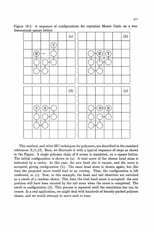
477

Figure 18.1: A sequence of configurations for reptation Monte Carlo on a two­dimensional s uare lattice

( a) (b)

(d) (c)

This method, and other MC techniques for polymers, are described in the standard references [3,11,12). Here, we illustrate it with a typical sequence of steps as shown in the Figure. A single polymer chain of 8 atoms is simulated, on a square lattice. The initial configuration is shown in (a). A trial move of the chosen head atom is indicated by a vector. In this case, the new head site is vacant, and the move is accepted, giving configuration (b). The same head atom is chosen again, but this time the proposed move would lead to an overlap. Thus, the configuration is left unaltered, in (c). Now, in this example, the head and tail identities are switched as a result of a random choice. This time the trial head move is accepted: the new position will have been vacated by the tail atom when the move is completed. The result is configuration (d). This process is repeated until the simulation has run its course. In a real application, we might deal with hundreds of densely-packed polymer chains, and we would attempt to move each in turn.

478

A measure of the 'size' of a polymer molecule is the mean-square end-to-end dis­tance < .C:!:rh >=< IrN - rll 2 >, where rl is the position of atom 1 and rN is the position of atom N in an N-atom chain. This can be calculated as a simulation aver­age in the usual way. It is interesting to compare this quantity with the predictions of a simple random walk theory. In this, atom 1 is placed at an arbitrary point on the lattice, atom 2 is placed, with equal probability, at any of the neighbouring lattice sites, atom 3 placed randomly next to atom 2 and so on. The result is an N-step random walk, taking no account of the exclusion effects (Le. sites can be multiply occupied). In a simple one-dimensional case, each site having two neighbours, the exact mean-square displacement is < C:!.rh >= N, taking the lattice spacing as unity. What is the result in two dimensions?

18.3 Task

Write a reptation Monte Carlo program for this system. Consider just one chain of about 8 atoms moving on a lattice. Choose the initial configuration in any way you like, making sure that no overlaps are allowed. In the simulation, move the head atom in any of the three 'non-backwards' directions. Measure the mean-square end-to-end distance as a simulation average. Compare with the simple random walk prediction.

18.4 Further work

• Repeat the exercise, but include the effects of a solvent by introducing obstacles: non-moving atoms that simply block one site each. The chain must wind its way in between the obstacles: the head atom can only move to vacant sites. Choose a density of obstacles by trial and error, and distribute them randomly, making sure again that there are no initial overlaps with chain atoms. Make sure that you don't exceed 50% occupation of sites by obstacles (why?). Compare the mean-square end-to-end distance with your first results.

• Repeat the original exercise, but start from a configuration in which every bond angle is a right angle (i. e. there are no straight-line sections) and only allow head atom moves to be at right angles to the existing bond (i. e. no 'backwards' or 'forwards' moves). Compare results.

• Consider trying out reptation Monte Carlo on a triangular two-dimensional lattice (every site has 6 neighbours) and on a three-dimensional cubic lattice.

• Tryout this method for a dense system of many polymer chains, attempting to move each in turn.

479

19 Simulations of crystal surfaces

19.1 Summary

This project involves using the solid-on-solid model to simulate the surface of a crys­tal, using various Monte Carlo techniques. Special emphasis is placed on considering the requirements of microscopic reversibility, and the devising of kinetic Monte Carlo schemes. This project would be suitable for an individual, or for a team, each indi­vidual pursuing a different aspect.

19.2 Background

The computer simulation of crystal growth is a huge field of research (see [48] and references therein). Here we look at one of the simplest simulation models. The solid-on-solid (SOS) model can be thought of as a modification of the basic Ising or lattice gas model of statistical physics. It is specifically designed for the study of the interface between two phases [49,50). As in the lattice gas model, each site of a simple cubic lattice (let us say) is either unoccupied or occupied by an atom. There are nearest-neighbour interactions between atoms. However, in addition, one direction (the z direction, say) is singled out. At sufficiently large, negative, values of z, all the lattice sites are taken to be occupied; at sufficiently large, positive, z, all the sites are unoccupied. For each value of x, y, there is just one value of z at which the changeover from occupied to unoccupied takes place. In other words, there are no 'bubbles' of one phase included in the other, and no 'overhangs'. The system is a set of columns of atoms, based on the 2-dimensional square x, y lattice: for each x, y

lattice site, labelled i, let the height of the column be hi. This set of heights specifies the state of the system.

The energy can be written in several ways, but we choose the simplest:

E=E L Ihi-hjl· <ij>

(19.1 )

Here E is an energy parameter. The sum is over distinct nearest neighbour sites in the square lattice (i.e. neighbouring columns). We count the interaction between each site i and each of its four neighbours j only once. The heights are measured from an arbitrary origin: note that shifting them all by the same amount does not change E. Thus, the absolute position of the surface is not relevant. However, when we consider driving the process of crystal growth, the rate of change of the average surface position < h > will be of interest. Here the average < ... > is taken over all the columns. The surface width W is important. We can define this as the root-mean-square deviation of hi from the mean,

W =< (h- < h »2 >1/2 . (19.2)

480

This system exhibits a phenomenon called surface 'roughening': above a critical temperature ( kTR / e ~ 1.15) the surface becomes rough and ill-defined, and the width diverges.

19.3 Metropolis Monte Carlo

It is relatively easy to write a Metropolis Monte Carlo program to simulate the SOS model. To change the state of the system, we must change the values of the hi, typically by one unit at a time. A simple scheme is:

• select a column i (sequentially or at random);

• decide whether to try to increase or decrease hi;

• calculate a transition probability for this change;

• choose to make the change or not, according to this probability.

For simplicity, let us choose to increase or decrease hi with equal probability. Then, from eqn (19.1), it is easy to calculate the energy change tlE associated with such a move. The Metropolis formula [18] for the probability of accepting the move is

P(tlE) = min(l, exp( -tlE/kT)) (19.3)

where T is the temperature and k Boltzmann's constant. In other words, if tlE is negative (downhill), accept the flip unconditionally; if tlE is positive (uphill), accept with probability exp( -tlE/kT). As always, accepting a flip 'with a given probability' entails choosing a random number uniformly from a given range, typically (0,1).

Write a program to simulate a small (say 6 X 6 columns) SOS system using this method. Apply the usual periodic boundary conditions in the a: and y directions. You may find it useful to work in reduced units, setting e = 1. For simplicity, you can select columns for moves in a sequential way. Suggested input is as follows.

• The initial configuration (read in from a file, which you could prepare using the editor ).

• The temperature, in reduced units, kT / e.

• The run length in Monte Carlo cycles (one cycle is one attempted move per column).

The NAG library provides random number generators: the subroutine G05CCF initial­izes the generator in a non-reproducible way, while the function G05CAF ( DUMMY )

returns a random number in the range (0,1). Both G05CAF and its dummy argument DUMMY should be declared DOUBLE PRECISION. Suggested output at user-specified in­tervals:

481

• The total energy.

• The average height < h > (just to check for drift).

• The interface width, defined by eqn (19.2).

• The ratio of moves accepted to moves attempted.

Run the program, starting from a flat surface, choosing temperatures above and below the approximate roughening temperature mentioned above.

19.4 Transition probabilities

It is instructive to consider the operation of the Metropolis method in more detail. Two kinds of move are contemplated. Increasing a column height hi -+ hi + 1 means creating a new atom at the vacant 3-dimensionallattice site just above the top of the column. Depending upon the heights of neighbouring columns, this vacant lattice site might have from 0 to 4 neighbours in the lateral directions: call this number n. The energy change that goes into the Metropolis prescription depends on n. Referring to eqn (19.1), calculate this energy ll.E:; for each n (it also depends on € of course). The converse process, decreasing a column height hi -+ hi - 1 corresponds to annihilating an atom from the top of a column. This atom might have from 0 to 4 lateral neighbours, depending on neigbouring column heights. Calculate ll.E;;, the associated energy change, for each n. You should have, of course, ll.E:; = -ll.E;;, since one process is the reverse of the other. You should also note that, for a site with exactly two lateral neighbours, ll.Et = -ll.E; = o. These are called 'kink sites': at equilibrium they can be created or destroyed freely.

The transition probability II; is a product of two terms. One is the underlying probability of selecting a certain trial move, a;, and we have been taking all these to be equal, for simplicity: a~ = a;; = a for all n. The other is the Metropolis function, eqn (19.3), giving the probability of accepting such a move. In this case P; = min(l,exp(-ll.E;/kT)). So we have II; = a;P; and (to account for the possibility that all the a's are not the same in general) microscopic reversibility applies to the II functions. Here, this means

II+ II~ = exp( -ll.E:; /kT)

n (19.4)

Now draw up a table of Boltzmann factors and transition probabilities for creation and annihilation moves, as functions of n. Your probabilities should satisfy eqn (19.4). At this point, you may wish to check your table with a tutor.

Having gone through this exercise, you probably realize that the heart of your Monte Carlo program can be speeded up. For each attempted move, creation or an­nihilation, you only require to calculate the appropriate number of lateral neighbours. The expensive exponentials can be pre-calculated, and looked up in a table. You may wish to make this change, and see if any speed improvement results.

482

19.5 Varying the prescription

Now we can try changing the basic Metropolis prescription. This is where things become interesting, because we can seek to make the Monte Carlo method model what actually happens in the real system, albeit in an idealized way.

Suppose that we wish to make the rates of selection and acceptance of creation moves independent of site, while the annihilation of atoms continues to depend on the binding energies with neighbours. This corresponds to a simple model of crystal growth: atoms arriving from the liquid add on to the growing surface irrespective of their environment, but to remove an atom it is necessary to break the bonds with its neighbours. We can arrange this in our Monte Carlo simulation, but must pay attention to microscopic reversibility. Thus we can set P; = P+, a constant for all n. In fact, we can make this constant unity if we like, accepting every creation move that we attempt; we shall probably have to attempt such moves less often. Certainly, the underlying transition matrices for creation and annihilation will have to be different. We can set a;t = a+ and a~ = a- for all n, where a+ f= a-. Finally, the annihilation move acceptance probabilities must be determined by the microscopic reversibility condition, eqn (19.4). Draw up a table, as you did in the last section, giving transition probabilities for both kinds of move, for each value of n, using this scheme. Check (for example) that the rates of kink site (n = 2) creation and annihilation are equal. If you like, adapt your simulation program along these lines. Consider one point: move acceptance probabilities cannot be greater than unity. Do you need to take any special measures to ensure this?

Suppose that we wish never to reject a move: at each site, we consider only increasing or decreasing h. Now the distinction between attempting moves and ac­cepting moves is blurred. We select a site, and calculate two weights: one for creation and one for annihilation. Then, we use the weights, and a random number generator, to decide between these two possibilities. Consider more carefully how to construct this scheme, without violating microscopic reversibility. Note that there will be two separate sets of energy changes involved in the two possibilities: the creation and annihilation moves being considered are not the reverse of one another.

19.6 Kinetic Monte Carlo

In kinetic Monte Carlo, we drive crystal growth (or the reverse process) by scaling all the creation probabilities with respect to the annihilation probabilities. Now the rates of kink site (n = 2) creation and annihilation are not equal; instead they are related by

ITt = exp(AIL/kT)IT2" (19.5)

where AIL represents a chemical potential difference (zero at equilibrium). The rest of the probabilities are shifted in the same way. Incorporate this modification in your program. Now the crystal will grow (if AIL > 0), and you can measure the growth rate (by monitoring < h > ) as a function of T and AIL.

483

19.7 Further work

This project can be taken in several directions. Much useful information on crystal growth simulations can be found in Muller-Krumbhaar's review [48], and the refer­ences therein. Here are a few possibilities.

• Study the growth of screw dislocations. This requires some modification of the boundary conditions, and you might like to consider how to change your program to handle this.

• Start the simulation from an irregular surface, or one with a specific defect or feature, and compare the evolution with that from a flat surface.

• Use different underlying lattices, to model the growth rates of different faces of a crystal.

Finally, demonstration programs for the SOS model are available on the DAP: try running them to see some of the features of this model.

20 Irreversible aggregation by Brownian dynam­ics simulation

20.1 Summary

This is an introduction to Brownian Dynamics, BD. In this exercise you will run a simple 3-dimensional BD simulation program that generates a "suspension" of Lennard-Jones, LJ, macromolecules in a fluid. You have to include the pair radial distribution function in the program and monitor the fractal dimension of the devel­oping aggregates as a function of time.

20.2 Background

The object of this exercise is for you to learn about a method to model macromolecules in solution using the technique of Brownian Dynamics, BD [51,52]. It is very similar to Molecular Dynamics, MD.

Molecular Dynamics in its simplest form, i.e. for a system at equilibrium, is simply a numerical solution of Newton's equations of motion,

R(t) = F(t)/m. (20.1)

where R is the position of an arbitrary molecule chosen out of N, m is the mass of the molecule (for simplicity, they all have the same mass here) and F is the net force on the molecule. For the a: component of the force, F.,(t) at time t then,

F.,,' = _ ~ (o¢( r ) ) r .,ii , ( ) L.J or r.. 20.2 ifi r=r,; '3

484

where rij = ~ - R j • The subscript, i, denotes the molecule index and ~ is the position of molecule, i. In this work we will assume pairwise additive interactions of the form ¢J(r). The Lennard-Jones potential, [53]

(20.3)

is a popular choice, which we will use here. If we are interested in suspensions of particles in a liquid then the details of

the comparatively fast movements of the 'solvent' molecules are not going to have a bearing on the movements of the large molecule, except in some kind of 'average' sense. This 'mean-field' approximation we can treat as follows. For particles rv Ip,m in diameter then the Langevin equation is a reasonable governing equation for this situation,

R(t) = F(t)/m + S(t)/m - ,8It(t), (20.4)

where S(t) is an 'instantaneous' random force intended to approximate the resultant effect of the 'collisions' of the many millions of host fluid molecules on the macro­molecule of interest. When we say 'instantaneous' here we mean 'instantaneous' on the time scale of the macromolecules (i.e. a time span in which they hardly move ) whereas this can be a very long time indeed for the host fluid molecules. (Very long compared to the lifetime of their time correlation functions.) The force S(t) is the net result of the buffetings of the host fluid molecules upon the macromolecule during this small time for the macromolecule but long time for the host molecule. The solvent has another effect which is incorporated in the last term on the right hand side of eqn (20.4). This is a Stokes drag term, representing the resistance of the host medium to the 'flow' of the macromolecule. The Stokes friction coefficient, ,8, is defined as,

(20.5)

where TJ. is the viscosity of the pure solvent. A finite difference algorithm is used to evolve the particles according to eqn (20.4).

In fact, the particles should move continuously through space with time, t, given any preset equations of motion governing the particles. This is worth bearing in mind! There are N LJ molecules in the BD cell. The positions of the molecules, R, in FORTRAN program ljbd, are updated in time steps of duration, h, using a leapfrog algorithm, [53], of the form,

R",(t + h) = R",(t) + .6.R",(t), (20.6)

for the x-component of R", where we have, [53]

.6.R",(t) = (F",(t) + S",(h))h/,8m, (20.7)

where h is the time step and

< S;(h) >= (2kB Tm,8/h). (20.8)

485

Now some technical details. The BD simulations are performed on a cubic unit cell of volume V . LJ reduced units are used throughout the program, i.e. kBT/€ -+ T, and number density, p = N 173 /V. Time is in u( m/ € )1/2. The program prints out Tp = j3-1, the time for relaxation of macromolecular momentum,

Tp = m/37ru"l., (20.9)

and also, T~, the time for significant structural evolution, i.e. movements of the macromolecules rv 17,

(20.10)

20.3 The problem

• I would like you to modify program Ijbd to include the calculation of the pair radial distribution function, g(r),

g(r) = n( r )/( 47rpr2 dr). (20.11)

where n( r) is the average number of particles found in the annulus r - dr /2 < r < r + dr /2 about an arbitrary particle.

• Take T = 1.0 and p = 0.6 for the state point. Also, in the first instance, N = 32 and run each simulation several times from different starting configurations to assess the statistical noise. Let me know if you run into problems so I can give you some help!

• Once you have written the program and equilibrated your dispersion at the above state point, reset the state point to, T = 0.2 and p = 0.1 to look at irreversible aggregation. At this low temperature and density the LJ particles will "stick-together" more or less on contact. The small clusters will grow into larger clusters in some fashion.

Why not calculate the fractal dimension D J of the aggregates?

g(r) '" rDrd, (20.12)

for r -+ 00, where d is the dimension of the space (= 3 here). The clusters formed should have a fractal dimension D J of 2.5 if they form by particle-cluster aggregation and should be 1.78 ifthey form by cluster-cluster aggregation [54]. Good luck!

21 Diffusion-limited aggregation

21.1 Summary

Write a program to grow a crystal in two dimensions using diffusion limited aggre­gation. The simulation is performed on a two-dimensional square lattice. Calculate the fractal dimension of the crystal.

486

21.2 Background

The word fractal is derived from the latin word fractus which means irregular or fragmented. It was used by B. Mandelbrot [55] to describe a class of objects where the dimension can be, and often is, non-integer. We are used to Euclidean objects such as the sphere where the dimension is 3. What we mean by this is that the volume (V) ofthe object scales as the third power of a linear dimension (L) such as the diameter. However not all objects are as well behaved as this. The Sierpinski sponge [56], shown in figure 21.1, is constructed by dividing the face of the cube into nine smaller squares. The central square on each face, and the plug of material behind, is removed through to the opposite face. The construction is repeated on each of the eight remaining smaller squares and so on ad infinitum. The picture shows this construction taken to the third level. For this sponge V(L) scales as L D , where D the fractal dimension is 2.7268. The sponge illustrates another important feature of fractal objects which is their self similarity, i.e. when the object is studied at a microscopic level it has the same structure or pattern as the object viewed at a macroscopic level. These fractal structures are not merely mathematical nightmares, since approximations to them are common in nature. An area where the fractal concept is useful is that of aggregation or cluster growth, e.g. in the electrodeposition of zinc metal leaves on a surface [57].

One interesting model of cluster growth is diffusion limited aggregation [58]. A dynamic simulation of this model might proceed by placing a seed particle on a square lattice. A second particle is fired at the seed from a lattice point close to the firing circle (FC) and it executes a random walk on the lattice. If it explores a lattice point adjacent to the seed particle, it sticks and forms part of the growing cluster. If it crosses an escape circle (EC), some distance outside the firing circle, the walk is terminated and the particle is started again from a random lattice point on the the firing circle. A second and subsequent particle sticks if, after firing, it becomes adjacent to any particle already in the cluster. As the cluster grows the firing circle and the escape circle have to be moved back so that during the simulation FC is approximately five lattice spacings from the outside edge of the cluster. A typical run might comprise 3000 to 5000 shots. The geometry of the simulation is shown in figure 21.2.

21.3 Task

Write a program to grow a cluster using the DLA mechanism on a two-dimensional square lattice. You will need to choose a lattice size for your problem, and positions for the firing and escape circles. Draw out the cluster at intervals of 1000 shots. It is interesting to colour or mark shots in the intervals 1-1000, 1001-2000, etc, in different way, so that in your final picture we can establish where particular particles finish within the cluster as a function of the firing time. Calculate the fractal dimension of the patch by calculating the number of particles N( r) inside a circle of radius r

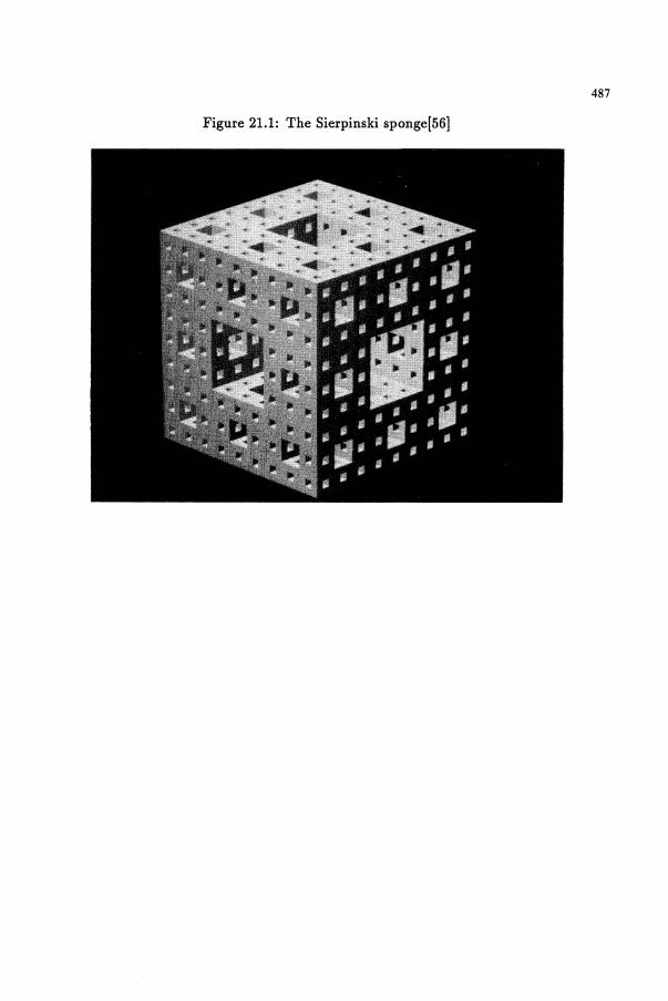
487

Figure 21.1: The Sierpinski sponge[56]

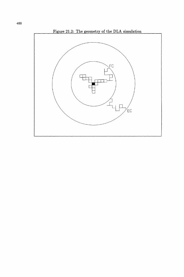
488

FC

T~ EC

489

centred at the seed. A log-log plot of N(r) against r should contain a linear portion where the slope is the fractal or Hausdorff dimension.

21.4 Further work

• Is the cluster really fractal, i.e. is it self similar on all length scales? Can any objects in nature be completely fractal in this respect?

• Repeat the exercise, using a triangular lattice in two dimensions. Does the shape of the lattice affect the fractal dimension of the cluster?

• Change the sticking probability of particles, i.e. allow particles to stick with a probability of 0.5. You will need to make decisions about what to do with particles which do not stick to the lattice at the first attempt. How does this change the fractal dimension of the patch?

• Design an algorithm which allows you to fire particles in straight lines to the cluster. This simulation will model cry tal growth from a two-dimensional gas rather than a two-dimensional liquid. What is the fractal dimension of this patch? .

22 Shear flow in 2D Lennard-Jones fluid by non­equilibrium molecular dynamics

22.1 Summary

This task is an introduction to Non-Equilibrium Molecular Dynamics, NEMD. In this exercise you will work with a simple MD simulation program that generates a 2-dimensional Lennard-Jones, LJ, fluid. You will modify it to introduce shear flow (here, "plane couette flow") and thereby calculate the shear viscosity.

22.2 Background

The object ofthis exercise is to get some practice at writing a simple Non-Equilibrium Molecular Dynamics, NEMD, simulation program.

First, the essentials of the equilibrium program you will be working with are given below. A finite difference algorithm is used to evolve the particles according to slightly modified Newton's equations of motion. In fact, the particles should move continuously through space with time, t, given any preset equations of motion governing the particles. This is worth bearing in mind! There are N LJ molecules in the MD cell. The positions of the molecules, R, in FORTRAN program lj2d, are

490

updated in time steps of duration, h, using the leapfrog formulation of the Verlet algorithm, [59]

and Ry(t + h) = Ry(t) + ARy(t),

where at constant total energy we have, [59]

AR",(t) = AR.,(t - h) + F",(t)h2Im,

ARy(t) = ARy(t - h) + Fy(t)h2 Im,

(22.1)

(22.2)

(22.3)

(22.4)

where F",(t) and Fy(t) are the forces on a molecule at time t and m is the mass of the molecule (for simplicity, they all have the same mass here).

F",i = -~ t (otf;(r)) r"'ij , m.. or 1''' ''/-3 r=rij '3

(22.5)

where rij = Ri - Rj. The subscript, i, denotes the molecule index and Ri is the posi­tion of molecule, i. At constant temperature, T, (which is essential for sheared fluids because they are continuously trying to warm up!) we can maintain the temperature constant using the so-called velocity rescaling method as first derived by Woodcock, [60]

AR",(t) = AR",(t - h) X K(t - h) + F",(t)h2 Im, ARy(t) = ARy(t - h) x K(t - h) + Fy(t)h2 Im.

(22.6)

(22.7)

The constant, K(t - h), is a scaling factor, which under shearing conditions, will on average be slightly less than unity.

(22.8)

where Ek(t - h) is the kinetic energy of the MD cell of particles,

1~. 2 Ek(t - h) = - L.. mR(t - h) ,

2 i=l (22.9)

where to an adequate approximation,

it = AR(t - h)lh. (22.10)

The MD simulations use particles interacting via the Lennard-Jones potential,

(22.11)

The MD simulations are performed on a square unit cell of area A. LJ reduced units are used throughout the program, i.e. kBT If. ---t T, and number density, p = N ()'3 IV.

491

Time is in u(ml f)1/2. Consequently, your shear rate is in (f/m)1/2 lu, shear viscosity is in (mf )1/2 I u2 and stress is in fU- 2.

The shear velocity profile, 1', is to be introduced in the fluid using isokinetic SLLOD equations of motion [61,62). The peculiar or thermal velocity is denoted by

v""

R., v., = v., + 1'Ry, (22.12)

Ry Vy = vy, (22.13) dv.,

F.,lm - 1'vy, (22.14) dt

dvy Fylm. (22.15)

dt

22.3 The problem

• I would like you to modify program Ij 2d to include a shear flow field. In addition to changing the program to include the extra terms in eqns (22.12)­(22.15), you will need to make the periodic boundaries of the cell compatible with the macroscopic shear velocity profile. We often use so-called Lees-Edwards periodic boundary conditions to achieve this [63). These are succinctly,

Ri ., k y

R., + niLy1', Ry ,

(22.16)

(22.17)

where the superscript i refers to the image of the particle whose position in the 'real' MD cell is R. The value of ni (the image index) in the y-direction ranges from -00 < ni < 00. The real MD cell corresponds to ni = O. The side length of the MD cell in the y direction is L y • The position displacements are

{R., + niLy1't}, Ry ,

(22.18)

(22.19)

where t is the time duration of the simulation since the application of the shear velocity ~eld. The notation { ... } is shorthand for: apply periodic boundary conditions so that R~ falls within the same limits as that of R", (i.e. 0 < R~ < L." where L., is the sidelength of the cell in the a: direction.). If the 'real' particle moves out of the cell, its image i enters at the position,

R., -+ {R., + niLy1't},

Rt -+ Ry + niLy

(22.20)

(22.21)

Let me know if you run into problems so I can give you some help! Take T = 0.5 and p = 0.75 for the state point (it is close to the 2D LJ triple point [63,64)). Also, in the first instance set, N = 50 and run each simulation several times to assess the statistical noise.

492

• Once you have written the program to generate the positions of the particles at fixed 1', then calculate the viscosity, "l, from

(22.22)

where 1'",ij is the x component of rij and A = (N / p), the area of the MD cell.

(22.23)

23 The Fourier transform and applications to mole ular dynamics

23.1 Introduction

The Fourier transform is one of the most important mathematical transforms. In molecular dynamics simulations it has many uses, some of which will be introduced here. It must be said that a brief introduction like this cannot hope to encompass more than a minute part of the subject, but what we cover will provide an outline of some of the commonest applications in MD. Students not acquainted with Fourier transforms should take time to read the following notes in preparation for the computational exercises to follow. We will deal with the following aspects.

• The definition of the Fourier transform

• Some mathematical properties of Fourier transforms

• Some examples of Fourier transforms

• The discrete Fourier transform

For further details refer to [65,66,67,68,69,70,71].

23.2 The Fourier Transform

We shall be concerned exclusively with the complex Fourier transform, since this is the most general form. There are few handicaps to this approach. Mathematically, we can write the Fourier transform H(f) of a function h(t) as:

H(f) = i: h(t)exp(-i27rft)dt (23.1)

and its so called inverse transform as:

h(t) = i: H(f)exp(i27rft)df (23.2)

493

The variables t and f are said to be conjugate variables in the time and frequency domains respectively. In this document we will refer almost exclusively to these variables, but they are not the only conjugate variables that commonly occur. Other examples are time, t, with angular frequency w = 27rf:

H(w) = i: h(t) exp( -iwt)dt (23.3)

h(t) = ~ /00 H(w) exp(iwt)dw 27r -00 (23.4)

and the position vector, r with the reciprocal space vector, k:

H(k) = i: h(r) exp( -ir.k)dr (23.5)

h(r) = {Lr i: H(k)exp(ir.k)dk (23.6)

The occurence of a Fourier transform and its inverse is dependent on certain math­ematical conditions. They are intuitively reasonable but require rigorous proof. Briefly, they assume that the integrals (areas) of the functions hand H over the range concerned exist and are are bounded, and that the functions take a mean value at any discontinuity. These are known as the Dirichlet conditions. It will be impor­tant to remember these in subsequent sections. Any good textbook on the subject will discuss these more fully.

23.3 Some Properties of the Fourier Transform

In order to use the Fourier transform as an effective mathelI1'l.tical tool, it is essential to know some of the basic properties. We present here "orne of these properties, which will be useful when tackling the exercises. They will be presented without proof, but students should attempt to prove them to their own satisfaction at their leisure. (Note: In what follows the Fourier transform of a function h(t) is indicated by H(f) = FT(h(t)) and the inverse Fourier transform by h(t) = FT-1(H(f)).)

23.3.1 Even, Odd and Ordinary Functions

A function f(x) of a variable x is even if f( -x) = f(x) and odd if f( -x) = - f(x). Ordinary functions do not have either of these properties. Using these definitions it can be shown that:

• An ordinary function is a sum of an even and an odd function.

• If h(t) is real and even then H(f) is real and even.

• If h(t) is real and odd then H(f) is imaginary and odd.

494

• If h(t) is real and ordinary then H(f) is complex with an even real part and odd imaginary part.

• If h(t) is imaginary and even then H(f) is imaginary and even.

• If h(t) is imaginary and odd then H(f) is real and odd.

• If h(t) is imaginary and ordinary then H(f) is complex with an odd real part and even imaginary part.

• If h(t) is complex and even then H(f) is complex and even.

• If h(t) is complex and odd then H(f) is complex and odd.

• If h(t) is complex and with an even real part and odd imaginary part then H(f) is real.

• If h(t) is complex and with an odd real part and even imaginary part then H(f) is imaginary.

23.3.2 Shift Theorems

Basically these show that a change in origin in one domain results in the appearance of a phase factor in the other domain. i.e.

• If FT(h(t)) = H(f) then FT(h(t - to)) = H(f) exp( -i27rfto).

• If FT-1(H(f)) = h(t) then FT-1(H(f - fo)) = h(t) exp(i27rfot).

23.3.3 Scaling Theorems

These theorems show that a change of scale in one domain results in the inverse scaling in the other. i.e.

• If FT(h(t)) = H(f) then FT(h(at)) = a-I H(f la).

• If FT-l(H(f)) = h(t) then FT-1(H«(3f)) = (3-1h(tl(3)

23.3.4 Parseval's Theorem

This important theorem provides a way of expressing the integral of the square of a function (say h(t)) in the time domain as an integral involving its Fourier transform (i.e. H(f)) in the frequency domain:

495

In the case where h(t) can be expressed as a sum of harmonic frequencies, this offers a very simple way of evaluating the l.h.s. integral, since the r.h.s. is then a simple arithmetic sum. It is useful in evaluating the power in a fluctuating function (wave­form) described by h(t). Parseval's theorem is a special case of a theorem concerning the product of two functions in the time domain.

23.3.5 The Convolution Theorem

Two of the most important properties of Fourier transforms concern the convolution integral and the correlation integral (below). A convolution integral has the form:

c(t) = J h(t')g(t - t')dt'

Which is a convolution of the functions h(t) and g(t). It is permissible for these two functions to be the same. The convolution theorem says:

• If c(t) is the convolution of h(t) and g(t) and these three functions have Fourier transforms a(f), H(f) and G(f) respectively, then

a(f) = H(f)G(f).

This powerful theorem shows how a difficult integral problem in one domain becomes much easier in the other domain. This has important computational advantages in certain problems.

23.3.6 The Correlation Theorem

Correlation integrals are very common in molecular dynamics. They form the basis for the analysis of time dependent phenomena. A correlation integral has the form:

c( t) = J h( t')g( t + t')dt'

Which is a correlation of the functions h(t) and g(t). If these two functions are the same, it is said to be an auto-correlation function. If they are different functions, it is called a cross-correlation function.

The correlation theorem says:

• If c( t) is the correlation function of h( t) and g( t) and these three functions have Fourier transforms a(f), H(f) and G(f) respectively, then

a(f) = H*(f)G(f),

where H*(f) is the complex conjugate of H(f).

This is a theorem of immense power, both in theoretical studies and computational algorithms.

496

23.3.7 The Wiener-Khintchine Theorem

This theorem has application in the analysis of time dependent correlation functions, where it sheds light on the frequency dependence of such phenomena as energy dis­sipation etc. It says that:

• If FT(c(t)) = C(f), where c(t) is a time dependent correlation function, then:

C(f) = 21000 c(t)cos(27rft)dt

• and conversely:

c(t) = 21000 C(f)cos(27rft)df

This follows quite simply if it is assumed that the correlation function is symmetric about t = O.

23.3.8 Derivatives of a Function

This provides the relationship between the derivative of a function and its Fourier transform. It is important because it helps in the solution of certain kinds of differ­ential equation. Let h(t) be a function of time and H(f) its Fourier transform.

• If h'(t) = fth(t) is the derivative of the function h(t), then:

FT( h'( t)) = i27r f H(f).

• If h" (t) = ft22 h( t) is the second deri vati ve of the function h( t), then:

Higher order derivatives have similar expressions.

23.3.9 The Dirac Delta Function

The Dirac delta function (which is not strictly a function at all), is a useful device for demonstrating certain properties of Fourier transforms and constructing formulae. It is sometimes referred to as the impulse function. It has the following properties:

• Ii (t - to) = 0 if t i:- to

• J~oo Ii(t - to)dt = 1

• J~oo h(t)li(t - to)dt = h(to)

where h( t) is an ordinary function. The function Ii( t) may be regarded as a rectangular function of vanishingly small width, but finite area (i.e. as a kind of sharp "pulse" function), though this is not a rigorous definition.

497

23.4 Some Example Fourier Transforms

We present here some examples of Fourier transformed functions. Any decent text­book on the subject will provide many more. The ones given have some relevance to the computational exercises outlined later.

23.4.1 Trigonometric Functions

1 FT( cos(27r lot)) = 2(5(1 + 10) + 5(1 - 10))

FT(sin(27r/ot)) = ~(5(1 + 10) - 5(1 - io))

The delta functions indicate that the continuous trigonometric functions in the time domain transform to single numbers in the frequency domain. This is an obvious example of the Fourier transform "projecting out" the frequency dependence of a function. Notice that the transform admits both positive and negative frequencies.

23.4.2 Gaussian Function

The gaussian function is common in all branches of physics, and molecular dynamics is no exception. If

then:

Notice the transformed function is also a gaussian.

23.4.3 Exponential Function

A function decaying exponentially from a fixed value at given time origin (assumed to be t = 0 here), is a common physical occurrence i.e.

h(t) = Aexp( -at), when t > 0

h(t) = A/2, when t = 0

h(t) = 0, when t < 0)

(Notice the definition of the function when t = 0, to comply with the Dirichlet conditions.) The Fourier transform is then:

498

Notice that the transform is complex. On the other hand, the double sided exponen­tial:

h(t) = Aexp( -alt!), with - 00 < t < 00

has the Fourier transform:

which is real.

23.4.4 Rectangular Window Function

This function is actually very common, although it is not often realised, particularly by novice users of the discrete Fourier transform. It is defined by:

wet) = A, when It I < T/2

wet) = A/2, when It I = T/2

wet) = 0, when It I > T/2

Where T is the width of the window in the time domain, and A is the height. Notice the second equation, which is necessary to define the discontinuity at It I = T /2 so that it satisfies the Dirichlet conditions. We then have:

W(f) = ATsin(7iTf)/(7iTf)

It is important to note that the Fourier transform is not an impulse function (5-function) in the frequency domain.

23.4.5 The Blackman-Harris Window Function

This function is used as an alternative to the rectangular window function described above. It is one of many alternative functions giving better resolution in harmonic analysis. It is defined by:

3

wet) = E aj cos(27ijt/T) j=O

where T is the width of the time window. The coefficients ao, . .. , a3 have the values 0.35875, -0.48829,0.14128 and -0.01168 respectively. Its Fourier transform is easy to obtain, but it is the convolution of this with the transform of the rectangular window function that is important. (It is designed to produce a good replica of the 5 function in the frequency domain).

499

23.4.6 The Dirac Delta Function

This follows easily from the definition of the delta function given above:

FT(A8(t)) = A

This shows that a spike at the origin in the time domain will give rise to a "plateau" in the frequency domain. If an unexpected plateau appears in any of your Fourier transforms, suspect this as the cause.

23.4.7 The Sampling Function

A continuous function in the time domain may be sampled by being multiplied by the following function, which samples at regular intervals tlt:

00

s(t) = L 8(t - jtlt) j=-oo

and its Fourier transform is:

S(J) =: f 8(J - j/tlt) ut. )=-00

This transform is central to the construction of the discrete Fourier transform.

23.5 The Discrete Fourier Transform

To convert the Fourier transform from its integral representation to a discrete rep­resentation amenable to digital processing, substantial modifications of the original time function are necessary. These modifications result in subtle changes in the prop­erties of the transform that affect the accuracy and interpretation of the result. It is instructive to examine these modifications in turn to see their effects and, where necessary remedy them. The principal modifications required are sampling and win­dowing in the time domain and sampling in the frequency domain.

23.5.1 Sampling in the Time Domain

The continuous function of time h( t) may be converted to a discrete representation by multiplying it by the sampling function s(t) described above. The sampling function consists of an infinite train of regularly spaced impulse functions of unit area and infinitesimal width separated by the time interval tlt. Multiplication by this function produces a set of data points equally spaced in the time domain at intervals of tlt, and weighted by the value of the function h(t) at the corresponding abscissa. Thus we have, in the time domain:

+00 h(t)s(t) = L h(ntlt)8(t - ntlt)

n=-oo

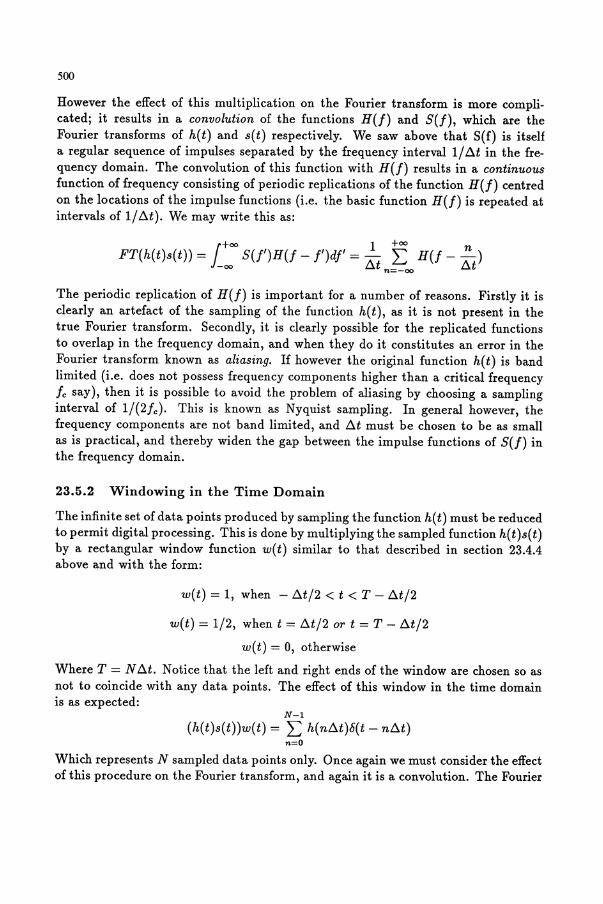
500

However the effect of this multiplication on the Fourier transform is more compli­cated; it results in a convolution of the functions H(f) and S(f), which are the Fourier transforms of h(t) and s(t) respectively. We saw above that S(f) is itself a regular sequence of impulses separated by the frequency interval 1/l1t in the fre­quency domain. The convolution of this function with H(f) results in a continuous function of frequency consisting of periodic replications of the function H(f) centred on the locations of the impulse functions (i.e. the basic function H(f) is repeated at intervals of 1/l1t). We may write this as:

(+00 1 +00 n FT(h(t)s(t)) = J- oo S(f')H(f - !')d!' = I1t n~oo H(f - I1t)

The periodic replication of H(f) is important for a number of reasons. Firstly it is clearly an artefact of the sampling of the function h(t), as it is not present in the true Fourier transform. Secondly, it is clearly possible for the replicated functions to overlap in the frequency domain, and when they do it constitutes an error in the Fourier transform known as aliasing. If however the original function h( t) is band limited (i.e. does not possess frequency components higher than a critical frequency Ie say), then it is possible to avoid the problem of aliasing by choosing a sampling interval of 1/(2/e). This is known as Nyquist sampling. In general however, the frequency components are not band limited, and I1t must be chosen to be as small as is practical, and thereby widen the gap between the impulse functions of S(f) in the frequency domain.

23.5.2 Windowing in the Time Domain

The infinite set of data points produced by sampling the function h(t) must be reduced to permit digital processing. This is done by multiplying the sampled function h(t)s(t) by a rectangular window function w(t) similar to that described in section 23.4.4 above and with the form:

w(t) = 1, when - I1t/2 < t < T - I1t/2

w(t) = 1/2, when t = I1t/2 or t = T - I1t/2

w( t) = 0, otherwise

Where T = N I1t. Notice that the left and right ends of the window are chosen so as not to coincide with any data points. The effect of this window in the time domain is as expected:

N-l

(h(t)s(t))w(t) = L h(nl1t)6(t - nl1t) n=O

Which represents N sampled data points only. Once again we must consider the effect of this procedure on the Fourier transform, and again it is a convolution. The Fourier

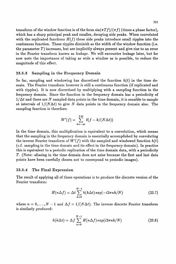
501

transform of the window function is of the form sin( 7rT f) / (7r f) (times a phase factor), which has a sharp principal peak and smaller, decaying side peaks. When convoluted with the replicated functions H(f) these side peaks introduce small ripples into the continuous function. These ripples diminish as the width of the window function (i.e. the parameter T) increases, but are implicitly always present and give rise to an error in the Fourier transform known as leakage. We will encounter leakage later, but for now note the importance of taking as wide a window as is possible, to reduce the magnitude of this effect.

23.5.3 Sampling in the Frequency Domain

So far, sampling and windowing has discretised the function h(t) in the time do­main. The Fourier transform however is still a continuous function (if replicated and with ripples). It is now discretised by multiplying with a sampling function in the frequency domain. Since the function in the frequency domain has a periodicity of 1/ tlt and there are N sampled data points in the time domain, it is sensible to sample at intervals of 1/(N tlt) to give N data points in the frequency domain also. The sampling function is therefore:

+00 W'(f) = L 5(f - k/(N tlt))

k=-oo

In the time domain, this multiplication is equivalent to a convolution, which means that the sampling in the frequency domain is essentially accomplished by convoluting the inverse Fourier transform of W'(f) with the sampled and windowed function h(t) (c.f. sampling in the time domain and its effect in the frequency domain). In practice this is equivalent to a periodic replication of the time domain data, with a periodicity T. (Note: aliasing in the time domain does not arise because the first and last data points have been carefully chosen not to correspond to periodic images).

23.5.4 The Final Expression

The result of applying all of these operations is to produce the discrete version of the Fourier transform:

N-l

H(ntlf) = tlt L h(ktlt) exp( -i27rnk/N) (23.7) k=O

where n = 0, ... , N - 1 and tlf = 1/(N tlt). The inverse discrete Fourier transform is similarly produced:

N-l

h(ktlt) = tlf L H(ntlf)exp(i27rnk/N) (23.8) n=O

502

It should be noted that these sums resemble the appropriate Fourier integral in each case, but in a form based on the rectangular sum approximation. (Warning: FFT routines available on most computing systems do not incorporate the normalisation constants At and Ai; users must therefore supply these values themselves.) The simple outcome eqn (23.8) is what leads novice users to believe that nothing much has happened to the Fourier transform in this process, but this account should convince the reader that this assumption is untrue. It is very important to realise that the discrete Fourier transform regards the time and frequency domain functions as being periodic in their respective domains, the first with periodicity T, given by the window width, and the latter with periodicity 1/ At, where At is the time domain sampling interval.

24 Harmonic analysis

24.1 Summary

The use of the Fourier transform in harmonic analysis is perhaps its best known application. In essence it is used to "project out" the underlying frequencies in a given function or signal. In this exercise, the student will apply the discrete Fourier transform to an harmonic analysis of a simple function. The exercise will show the problems that arise from an ill-considered application of the transform and reveal the usefulness of window functions. The object of the exercise is to familiarise the student with the behaviour of the discrete Fourier transform under controlled conditions. It is better to unravel the difficulties in cases where the results are known, than waste time mis-managing real experimental data!

Students should use the ID Fourier transform routine in the program library for this exercise. Note that this routine requires the processed arrays to be of length 2N ,

where N is an integer.

24.2 Background

In harmonic analysis we are primarily concerned with the frequency components of a "signal" of some kind. In molecular dynamics for instance, we might analyse the fluctuations in the values of some property or other, to determine the times cales of the fluctuations and their power spectrum. In principle the signal may be of infinite duration, in which case the harmonic analysis in integral form is given by:

H(f) = )~~ ~ i: h(t)exp( -i27rit)dt

503

but in practice, the signal is necessarily of finite duration and is sampled discretely. In this case the discrete form is employed:

ilt N-l

H(nilJ) = T L h(kilt)exp(-i2'Tmk/N) k=O

where T represents the time window over which the signal is sampled. (Note that since T = N ilt the normalisation factor is just l/N.)

The harmonic analysis generally yields a complex function of frequency, but this merely means that both the amplitude and phase information are present in the transform. We can separate these two parts quite simply: recall that any complex number can be written as the product of a real number and an imaginary power of e:

(a + ib) = Aei6

where A = (a2 + b2)1/2 and 8 = tan-1(b/a). So in harmonic analysis the amplitude of a frequency component is obtained by multiplying the H(nilJ) by its complex conjugate and taking the square root of the result. The phase is obtained from the inverse tangent of the ratio of the imaginary and real parts of H(nilJ). We may also combine the positive and negative frequency components if we wish, to obtain a real result.

The major difficulty with the harmonic analysis of an unknown signal is the problem of "leakage", whereby alien frequencies are introduced into the resultant spectrum by the discrete Fourier transform itself. It is more likely to be a problem than "aliasing", which is more evident in short duration signals, which necessarily contain very high frequencies. (This fact derives from the "uncertainty principle", in which a signal that is located precisely in the time domain (i.e. of short duration) is widely dispersed in the frequency domain (i.e. has a broad spread of frequencies).)

24.3 Task

Consider a cosine function with a periodicity P of 8 seconds i.e.:

h(t) = cos(27rt/P)

Suppose we have sampled this function at regular intervals ilt of 1 second over a time period T of 32 seconds (i.e. T = 4P). Construct an array of these data and use a discrete Fourier transform routine to obtain the Fourier transform. Does the result compare with the analytical result in Section 23.4.1? If it does not, do not proceed until you are completely satisfied with the results!

The second task is a repetion of the first, but with a small difference. Now set the period P of the cosine function to be 9.14, but retain the sampling interval of 1 second and the sampling period T of 32 seconds. What does the discrete Fourier transform produce in this case? Plot the function over the complete time interval

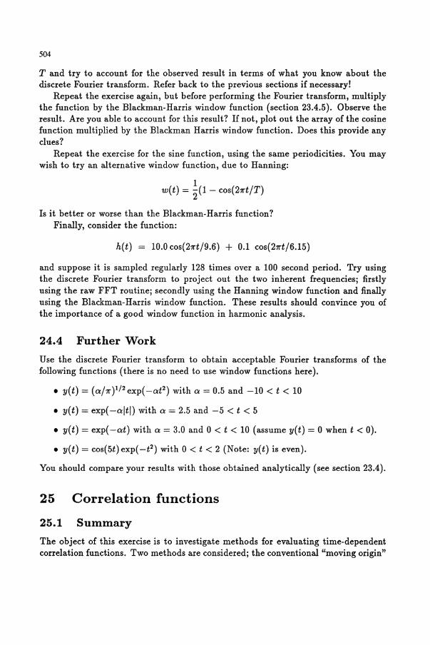
504

T and try to account for the observed result in terms of what you know about the discrete Fourier transform. Refer back to the previous sections if necessary!

Repeat the exercise again, but before performing the Fourier transform, multiply the function by the Blackman-Harris window function (section 23.4.5). Observe the result. Are you able to account for this result? If not, plot out the array of the cosine function multiplied by the Blackman Harris window function. Does this provide any clues?

Repeat the exercise for the sine function, using the same periodicities. You may wish to try an alternative window function, due to Hanning:

1 w(t) = 2(1 - cos(27rt/T)

Is it better or worse than the Blackman-Harris function? Finally, consider the function:

h(t) = 10.0 cos(27rt/9.6) + 0.1 cos(27rt/6.15)

and suppose it is sampled regularly 128 times over a 100 second period. Try using the discrete Fourier transform to project out the two inherent frequencies; firstly using the raw FFT routine; secondly using the Hanning window function and finally using the Blackman-Harris window function. These results should convince you of the importance of a good window function in harmonic analysis.

24.4 Further Work

Use the discrete Fourier transform to obtain acceptable Fourier transforms of the following functions (there is no need to use window functions here).

• y(t) = (a/7r)1/2 exp(-ae) with a = 0.5 and -10 < t < 10

• y(t) = exp( -altl) with a = 2.5 and -5 < t < 5

• y(t) = exp(-at) with a = 3.0 and 0 < t < 10 (assume y(t) = 0 when t < 0).

• y(t) = cos(5t)exp(-e) with 0 < t < 2 (Note: y(t) is even).

You should compare your results with those obtained analytically (see section 23.4).

25 Correlation functions

25.1 Summary

The object of this exercise is to investigate methods for evaluating time-dependent correlation functions. Two methods are considered; the conventional "moving origin"

505

method and a method based on the fast Fourier transform. The student should acquire some idea of the relative merits of these methods and gain some practice at coding them in a simple application. Students should use the ID Fourier transform routine in the program library for this exercise. Note that this routine requires the processed arrays to be of length 2N , where N is an integer.

25.2 Background

In molecular dynamics simulations it is frequently of interest to evaluate correlation integrals of the form:

1 loT c(t) = lim -T u(r)h(t + r)dr T-+oo 0

where u(t) and h(t) are both functions of time. (They may be the same function if required.) Such functions reveal a cause-and-effect relationship between the functions u(t) and h(t), by which a change in u(t) manifests a change in h(t) at some time later.

In molecular dynamics the correlation integral is approximated by the discrete equation:

/ Ilt N-k-l ) c(kllt) = \ (N _ k) ~ u(nllt)h«n + k)llt)

where k = 0, ... , N - 1 and N Ilt is a time interval over which the the correlation function is required. (Note: the angular brackets indicate an ensemble average, which in this context means an average over many time origins.)

This direct method however is not necessarily the fastest way to proceed. The correlation theorem (section 23.3.6) suggests that the business of correlation is simpler in the frequency domain. It is also well-known that the discrete Fourier transform (often called the fast Fourier transform or FFT) can Fourier transform any given function extremely quickly. A more efficient scheme therefore suggests itself:

• Fourier transform u(t) and h(t); obtain U*(f) and H(f), (the asterisk indicates the complex conjugate).

• Multiply U*(f) and H(f) together, as required by the correlation theorem. Obtain C(f).

• Inverse Fourier transform C(f) to obtain c(t).

Using the discrete Fourier transform, the correlation function may be written as:

/ Ilt 2N-l (n) ( n) (21f'ink)) c(kllt) = \ (N _ k)(2N) ~ U* 2N Ilt H 2N Ilt exp 2.JV

where k = 0, ... , N -1 as before. Notice that the sum ranges over 2N and not N as might be assumed at first. In practice, it means that an array of N zeros is appended to the arrays U* and H. This is done to correct an overlap or end effect which arises

506

because we necessarily must sample both U· and H over some finite time period (T say) which results in a meaningful correlation function of period 2T. If we choose a time window of T in the discrete Fourier transform, the transform will incorrectly assume a periodicity of T for all the functions it encounters, including the correlation function. In consequence, it will overlap the correlation function with itself, leading to spurious results. Doubling the time interval to 2T removes this error.

25.3 Task

Write a FORTRAN routine to calculate the correlation function of two variables u( nilt) and h(nilt), where n = 1, ... ,10000. Take the correlation out to 100ilt. Use the tra­ditional method, with a new origin taken every lOilt. Use the routine in conjunction with a Lennard-Jones molecular dynamics program from the library and calculate the velocity autocorrelation function.

Next write a second routine, incorporating a Fast Fourier transform routine and calculate the same correlation function as above. Compare the two previous methods in terms of accuracy and speed. Try to find ways of improving the performance of both of these methods (e.g. can you vectorise either of them?) and try to decide which of them you would prefer in general applications.

25.4 Further Work

Suppose you have a dataset containing the accumulated results of a molecular dy­namics simulation. Each data record contains M of real numbers, each of which specifies the value of a variable in the simulation at the same timestep. There are N data records corresponding to each timestep in the simulation. Design a program that uses the fast Fourier transform routine to calculate any desired auto- or cross­correlation function or functions as selected by the user.

26 Particle density calculations

26.1 Summary

The calculation of the Fourier transform of the particle density has elements which arise in several important areas of computer simulation. At the simplest level it provides a description of the order in a system (i.e. the melting factor), and at a more advanced level it provides the route to the dynamic structure factor. It also has much in common with electrostatic calculations using the Ewald sum. The student should gain experience of coding these elements efficiently and some insight into versatility of the three dimensional Fourier transform.

507

26.2 Background

One of the most powerful insights into the structure of liquids provided by molecular dynamics is the calculation of the dynamics structure factor S(k, w). Among other uses it is central to the theory of neutron scattering. A principal part of the calculation of this function is the spatial Fourier transform of the particle density.

The particle density is defined by:

N

p(r,t) = Lb(r-ri(t)) i=l

and its spatial Fourier transform is:

N

p(k,t) = Lexp(-ik.ri(t)) i=l

where k is a reciprocal space vector, which for a cubic MD cell has the form:

t 271" ( ) k = L I,m,n

where I, m, n are integers and L is the width of the MD cell. (Note: there is an infinite set of functions p(k, t), though only the lowest orders of k are normally of interest.)

We may calculate a correlation function for each p(k, t) which is known as the intermediate scattering function F(k, t):

F(k, t) = (p(k, t)p*(k, 0))

This function may be calculated using a sum over origins. It is normally scaled so that F(k,O) = 1.

Finally, to obtain the dynamic structure factor, the intermediate scattering func­tion is Fourier transformed in the time domain:

S(k,w) = i: F(k,t)exp(-iwt)dt

The central importance of the Fourier transform in these calculations is manifest!

26.3 Task

Write a FORTRAN code that can be used to calculate the Fourier transform of the particle density, for a complete set of k vectors up to I, m, n values of (say) 5, suitable for processing the data provided by a typical atomic MD program every timestep. (Assume a cubic MD cell.) Test the routine by using it to analyse the periodicity in perfect crystals with face centred cubic, simple cubic and body centered cubic lattices. Find out if it possible to use the same routine with hexagonal lattices.

508

Can you adapt the routine to provide some method of indicating when a molecular dynamics simulation has melted?

Develop the code further to enable the calculation of the intermediate scattering function and the dynamic structure factor. On the basis of what you know about the correlation theorem (and assuming you have not yet exploited this) can you devise a way of proceeding directly to the dynamic structure factor, without calculating the intermediate scattering function first? (Unfortunately, because of the heavy amount of computing this kind of calculation entails, it will not be possible to test these developments fully.)

26.4 Further Work

Suppose that instead of point particles we had a system consisting of electrostatic charges represented by gaussian charge density distibutions:

where qi is the net charge on the i'th particle, and a is a parameter expressing the "width" of the gaussian function (note it is the same for all charges). Can you adapt the calculation of the Fourier transform of the particle density to calculate the Fourier transform of the charge density? What is the relationship between this calculation and the Ewald summation method for calculating the electrostatic contribution to the configuration energy?

27 Quantum simulations

27.1 Summary

Most dynamical simulations performed to date have used classical mechanics. Re­cently however much work has concentrated on quantum mechanical simulations, and it is likely that such simulations will grow in importance in the future. In this exercise the student will gain some experience of using a fairly simple quantum mechanical simulation method that is based on the discrete Fourier Transform. Its application to simple one-dimensional systems will provide some insight into the difficulties thai arise in quantum simulations, not only from the radically different approach that must be adopted, but from rationalising the results obtained.

27.2 Background

It is well known that the discrete Fourier transform may be used to solve differential equations. One particular application that has aroused much interest recently is its

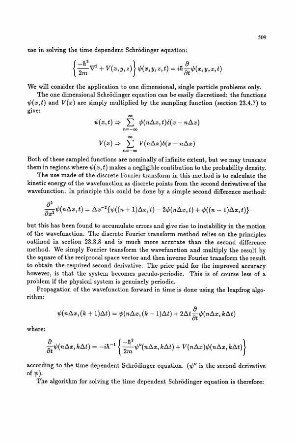
509

use in solving the time dependent Schrodinger equation:

{;~ V2 + V(x,y,z)}7fi(x,y,z,t) = ili;t 1fi(x,y,z,t)

We will consider the application to one dimensional, single particle problems only. The one dimensional Schrodinger equation can be easily discretized: the functions

7fi(x,t) and V(x) are simply multiplied by the sampling function (section 23.4.7) to give:

00

7fi(x,t) '* L 7fi(n!:l.x,t)5(x - n!:l.x) n=-oo

00

V(x) '* L V(n!:l.x)5(x - n!:l.x) n=-oo

Both of these sampled functions are nominally of infinite extent, but we may truncate them in regions where 7fi( x, t) makes a negligible contibution to the probability density.

The use made of the discrete Fourier transform in this method is to calculate the kinetic energy of the wavefunction as discrete points from the second derivative of the wavefunction. In principle this could be done by a simple second difference method:

82 8x2 7fi(n!:l.x, t) = !:l.x-2{7f1((n + l)!:l.x, t) - 27fi(n!:l.x, t) + 7fi((n - l)!:l.x, t)}

but this has been found to accumulate errors and give rise to instability in the motion of the wavefunction. The discrete Fourier transform method relies on the principles outlined in section 23.3.8 and is much more accurate than the second difference method. We simply Fourier transform the wavefunction and multiply the result by the square of the reciprocal space vector and then inverse Fourier transform the result to obtain the required second derivative. The price paid for the improved accuracy however, is that the system becomes pseudo-periodic. This is of course less of a problem if the physical system is genuinely periodic.

Propagation of the wavefunction forward in time is done using the leapfrog algo­rithm:

8 7fi(n!:l.x, (k + l)!:l.t) = 7fi(n!:l.x, (k - l)!:l.t) + 2!:l.t 8t 7fi(n!:l.x, k!:l.t)

where:

8 {_li2 } 8t 7fi( n!:l.x, k!:l.t) = -iii -1 2m 7fi"( n!:l.x, k!:l.t) + V( n!:l.x )7fi( n!:l.x, k!:l.t)

according to the time dependent Schrodinger equation. (7fi" is the second derivative of 7fi).

The algorithm for solving the time dependent Schrodinger equation is therefore:

510

1.

2.

3.

4.

5.

Discretize the starting wavefunction (at t = 0) and the potential function.

Calculate the wavefunction at timestep -llt using Runge-Kutta or alter­native method.

Calculate the second derivative of the wavefunction at each point.

Calculate the product V( nllx )7f'( nllx) for all points.

Propagate the wavefunction for one timestep according to the Schrodinger equation.

6. Renormalise wavefunction (if necessary).

Steps 3 to 6 are repeated for however many time steps are required. Note that the renormalisation in step 6 provides an additional measure of the stability of the algorithm (besides energy conservation). If the algorithm becomes unstable, the normalisation condition becomes seriously violated at each timestep.

27.3 Task

Take a copy of the program MDKOS from the library and examine it closely to famil­iarise yourself with the coding. Then run it with the following potential functions:

• A constant potential V = O.

• A parabolic potential V = ~k(x - xoY (find suitable values of k).

• A step potential: V(x) = OJ (x < L/2), V(x) = hj (x > L/2), where L is the width of the simulation cell, h is the barrier height.

• Any other potential that might interest you (e.g. double well potential).

Your objectives in each case should be:

• To cast the problem with the correct physical dimensions to ensure stability of the algorithm and an absence of artefacts.

• To rationalise the behaviour of the wavefunction in terms of quantum mechan­ics. (i.e. do you believe the results?)

27.4 Further Work

Extension of this method to more than one particle or dimension is difficult. However, it is possible to change the above method to deal with two interacting particles in one dimension without undue difficulty. Recognising that the two-particle one­dimensional system has only two degrees of freedom and the fact that the centre of mass of the system is not affected by the inter-particle interaction, can you work out how the adaptation can be made?

511

28 Percolation cluster statistics of ID fluids

28.1 Summary

In this exercise you will write a simple simulation program to produce a I-dimensional fluid. You will make use of it by investigating the distribution of clusters generated by the program. This leads to a probing of the long range connectivity of the fluid. If the fluid is "infinitely connected", it is said to percolate. The cluster statistics in the vicinity of the percolation threshold will be investigated by you, to test universal scaling relationships.

28.2 Background

The object of this exercise is to get some practice at writing a simple simulation program and applying it to a topical area of research.

In recent years there has been an interest in cluster distributions and cluster properties within simple fluids [72]. I would like you to look for clusters that extend over all space. (These are important in the "real world" because they determine the macroscopic behaviour of a number of weakly aggregating systems; the rigidity of gels and conduction through random networks, for example. Long-range connectivity in the largely-randomly positioned particles has a determining effect on the properties of these materials [73].) For this purpose, a cluster is defined as a group of molecules interconnected by an arbitrary coordination-distance. Above a certain density of particles in an infinite system there is a finite probability that clusters will form spanning all space. This is called a percolation transition or threshold. The density at which this occurs and the statistics and properties of the clusters in this region of the phase diagram are interesting because there are universal exponents that characterise them for non-interacting particles thrown randomly onto the sites of a lattice [74]. In lattice systems "universality" refers to the independence of the value of the exponents to the number of nearest neighbours or lattice coordination number. In calculations on off-lattice or continuum noninteracting disks [75] and spheres [76] the exponents are the same as those from the lattice simulations. Recent studies on continuum interacting fluids generated by Monte Carlo simulation suggest that the values of these exponents are the same for these assemblies, as well as being independent of the nature and range of the interaction potential. The fluids studied so far by MC simulation have been hard-spheres [77], square-wells [78] and adhesive-spheres [79].

Generally in percolation studies, a set of particles is considered to be part of the same cluster if each member is separated from at least one of the others by a distance::; u., which is arbitrary but is usually ~ u, the core diameter of the particle. A percolating cluster is a special cluster having infinite extent. Within the framework of the periodically repeating cells of your simulations, a sufficient criterion for percolation is for a particle and its image to belong to the same cluster. One parameter to vary is the ratio u./u and see what effect it has on the percolation

512

threshold and on the exponents. As this ratio diminishes to unity, we term this the soft-core to hard-core transition.

To maintain consistency with accepted notation, the density is given the symbol, p, here, rather than, p, as is usual for the reduced density of simple fluids. For an infinite number of molecules there is a well-defined density, Pc, at which there is a finite probability of finding a percolating cluster [80]. Above and below the percolation density many finite sized clusters exist. (As you will discover this transition is smeared for finite periodic systems.) These occupy the holes in the percolating cluster above Pc. The simulation methods employed in this exercise (e.g. [81]) will make use of these clusters. The distribution of different sized clusters is characterised by the cluster number distribution function, n., [82,83,84] which is the time-average number of clusters containing s particles, N. divided by N i.e. n. = N./ N. This is consistent with the definition used in other continuum works [76,82]. Note however that the cluster number definition used in lattice studies is pN./ N [74]. For finite periodic systems there is an upper bound on s, i.e. 1 ::; s ::; N.

The behaviour of lattice systems close to Pc is described in terms of the following critical exponents. In the discussion below we will use the value for the exponents taken from random population of 1D lattices. The summations involving n. will also only involve non-percolating clusters. Let e(p) be the "correlation" length scale ofthe largest cluster, then [80]

(28.1)

As v = 1.0 [80] then e diverges at Pc, approaching from either side and is typical of critical behaviour. In one dimension Pc = 1, the close packing density, and therefore it is only possible to probe the system for p < Pc' In the finite systems studied here the percolation transition is smeared out over a density range. As density increases from zero the fraction of configurations that generate a percolating cluster, P, increases from zero to unity. The larger the number of particles in the cell, N, then the narrower is the density range for this transition. The density at which P = 0.5 shows the smallest N dependence. The density at which P = 0.5 is best taken as the percolation threshold for that (N,r:r.) combination. As N increases we find

(28.2)

where L is the sidelength of the simulation cell and a is a positive constant. The next function we will consider is the zero'th moment of n •.

(28.3)

In ID a = 1.0 [80]. Here and for all the sums below we interested in the "singular" or nonanalytic part of the sum over all cluster sizes [80]. For each sum we must subtract off the analytic background. This is so we isolate that part of the sum dominated by the representative (i.e. largest) cluster in the vicinity of the percolation threshold. For completeness, there is a quantity called the percolation probability, P"", which is

513

the fraction of molecules found in the percolating cluster. It only applies for p ~ Pc [79,80]. In arbitrary dimension,

Poe ex: (p - Pcl. (28.4)

In one dimension f3 = 0.0 as p cannot exceed Pc [80]. In lattice studies this corresponds to the fraction of occupied sites belonging to the infinite percolating network. The susceptibility, X, is

(28.5)

where I = 1.0 in one dimension [80]. The "f" denotes the omission of the largest cluster at each sample configuration. The largest cluster discovered each time step can either be a percolating cluster, should one (or more) exist, or the largest non­percolating cluster (should there not be a percolating cluster). In polymer science the susceptibility, X, corresponds to the mass average molecular mass whereas E: sn.(p) corresponds to the number average molecular mass. Close to Pc,

(28.6)

for p ~ Pc. The functions f2, P 00 and X require finite-scaling corrections for these small peri­

odic systems, as discussed in the Appendix. At the percolation threshold [85],

n.(p) = n.(pc)J(z),z == (p - Pc)s";s ~ oo,p ~ Pc

(28.7)

(28.8)

where J(z) is a universal function and u = 1.0 in one dimension. In random lattice percolation the critical exponents are interrelated by scaling laws,

T = 2 + 1/8,u = l/(v + (3),2 - a = I + 2f3 = f3(8 + 1) = dv (28.9)

where d is the dimensionality (d = 1, here) [80,85]. T = 2 in one dimension.

28.3 The problem

• I would like you to make a contribution to our understanding of percolation by investigating the percolation cluster statistics of some simple 1-dimensional fluids.

- Hard-sphere fluid by random parking Monte Carlo

- Hard-sphere fluid by Molecular Dynan.lcs

- Hard-sphere fluid by Metropolis Monte Carlo

- Lennard-Jones fluid by Molecular Dynamics

514

Lennard-Jones fluid by Metropolis Monte Carlo

Soft-sphere fluid by Molecular Dynamics

Soft-sphere fluid by Metropolis Monte Carlo

Choose one of these and let me know so I can give you some help! A typical simulation program can be separated into the following parts.

- At the beginning there is a section for reading in control parameters (usu­ally from a separate dataset or file). These might include, for example in a MD program, the number of time steps to be calculated and the magnitude of the time step.

- Then the program has to decide upon the starting coordinates of the molecules (and velocities for MD). The molecules could start from a lat­tice and be given Maxwell-Boltzmann random velocities, or alternatively the molecular configuration and velocities could be read in from a dataset coming from a previous calculation. Note that at some stage you will have to start the molecules off from a lattice!

Now we arrive at the most time consuming part of the program. This is where we move the particles, either with time in MD or randomly in MC. In MD the force on every particle is evaluated by going through every pair interaction. In MC one usually evaluates the potential energy of a single particle moved one at a time. The periodic boundary conditions enter this part of the code. During this stage the expressions for the quantities in statistical mechanical ensemble averages are evaluated.

- Now we move the particles, all together in MD or (usually) one at a time in MC, for a single pass through the previous section. Again periodic boundary conditions need to be taken into account.

Once the desired number of passes has been completed, the calculation is closed down with the saving of molecular coordinates (and velocities for MD) onto a dataset, ready for future use in a resumed simulation. Other quantities, such as ensemble averages can also be carried over to the next simulation segment.

(If you want to save some time, use the FORTRAN program lj ld , which is a 1 dimensional Lennard-Jones Molecular Dynamics fluid program. Modify it to build in a percolation cluster search.) Have a look at the paper by Geiger and Stanley [82J who used Molecular Dynamics computer simulations to evaluate the percolation exponents of model liquid water. Take T = 1.0 and N = 50,100,200 .... and run each simulation several times to assess the statistical noise.

515

• Once you have written the program to generate the positions of the particles, calculate Pe( N) for 0'.10' = 1.1 and 1.5 by establishing the p at which P = 0.5. A percolating cluster in 1D is easy to find! If two particle centres are within 0'_ they are in a cluster together. If a third particle centre is within 0'_ of either of these two, then it also is in the same cluster, i.e. we now have a triplet. This procedure is continued. If a particle and its image are also in the same cluster, then within the repeating framework of periodic boundary conditions, all of space is part of a percolating cluster (i.e. we can 'hop' from one particle to the next and span all available space) .

• Determine X from eqn (28.5) and plot it versus P - PeeN) close to PeeN). Also test the 'laws' (28.7)-(28.9).

28.4 Appendix: Finite-scaling hypothesis

The finite-scaling hypothesis supposes that physical properties are homogeneous func­tions of the critical-coupling parameter,€ =1 (p - Pe(L»IPe(L) 1 and the length-scale of the system, L. First let us recall the notion of homogeneous functions in the case of two variables. If f(x,y) is a homogeneous function of two variables it obeys the following for an arbitrary constant, .x,

(28.10)

e.g. if f(x,y) = X 2y3, then c = -2a - 3b. By choosing .xb = y-l then f(x,y) can be rewritten as,

(28.11)

Returning to two cluster averages discussed in the text, Poo = f(€,L) and X = g(€,L) can be written in the homogeneous forms,

Poo = L-(3/vf(Ll /v€,l)

where c = (3, a = -1 and b = II, and

X = P/vg(L1/ V €,1)

(28.12)

(28.13)

where the quantity Ll/v€ ex: (LIOl/v from eqn (28.1) is therefore essentially a ratio of two lengthscales. In the limit, L ---t 00 and ~ «: L then Poo rv €(3 and X rv €-'Y. This indicates that feLl/v, 1) ---t (P/v€)f3 and g(Ll/v€, 1) ---t (P/v€t'Y in this limit. In the other limit, Ll/v € ---t 0, ~ ~ L then f and 9 must reduce to L-dependent constants.

29 Quaternions and constraints

29.1 Summary

This project compares two techniques for the simulation of small rigid molecules: the use of quaternion parameters to describe molecular rotation, and the introduction

516

of constraints into the atomic equations of motion. It is best attempted by a small team, divided into two subgroups, one to study each technique.

29.2 Background

Most molecules are legitimately regarded as being composed of atoms, held together by covalent bonds which are strong compared with the intermolecular interactions. While many interesting molecules are highly flexible, and none are truly rigid, it is considered a reasonable approximation in some cases to treat all the internal bond lengths and angles as being fixed. In this limit, the molecule becomes a rigid body. In classical mechanics we may treat it in either of two ways (and here it may be useful to refer to a standard text on Classical Mechanics, such as Goldstein [86]). We may separate the centre-of-mass translation from rotation about the centre of mass, and solve the associated equations of motion. The orientation of a molecule is represented by Euler angles [87,88] or, to avoid certain difficulties in the equation of motion, by quaternions [89]. Alternatively, we may solve the atomic equations of motion, imposing holonomic constraints upon the intramolecular separations, to fix the internal degrees of freedom. This gives rise to the SHAKE and RATTLE approaches [90,91]. Constraint dynamics is the more widely-applicable approach, since it can handle the case of flexible as well as rigid molecules. However, in the rigid limit, there seems to be little to choose between the two approaches. In comparing them, it is important to use similar underlying algorithms to integrate the equations of motion [92]. Historically, this has not always been the case: quaternions have been used in conjunction with Gear predictor-corrector methods, while constraints grew up with the Verlet algorithm (compare e.g. [36] with [93]). Here, we use similar low-order Verlet-like algorithms in both cases. Much of the background material can be found in the original references cited above, and in standard texts [3]. Here we present a summary only.

29.2.1 Quaternion algorithm

The rotational equations of motion of a rigid body may be treated as two first-order differential equations. One equation links the torque T acting on the body with the time derivative of angular momentum 1, and hence (via the moment of inertia) with the rate of change of the angular velocities

i' = T·. (29.1 )

The superscript s indicates that these vectors and time derivatives are measured in a space-fixed axis system. The second differential equation shows how the angular velocities determine the rate of change of the parameters characterizing the orienta­tion of the body. These in turn specify the rotation matrix A, used to convert from space-fixed to body-fixed axes thus:

eb = A.e·. (29.2)

517

The body-fixed frame is most conveniently chosen to diagonalize the inertia tensor, giving (for nonlinear molecules) three principal moments of inertia

(29.3) a a

and similarly for Iyy, I zz • The sum is over the atoms a in a molecule, ma is the atomic mass, and coordinates are measured from the molecular centre of mass. Then, 01£­diagonal elements being zero, angular velocity and angular momentum are linked by

l~ = I.,,,,.w~ (29.4)

and similarly for y and z. The conventional orientational parameters are the three Euler angles; for reasons

explained elsewhere [88,89] these can only be used at the expense of some difficulties in integrating the equations of motion. Instead, Evans [89] proposed the use of four quaternion parameters. The quaternions, for which we use the shorthand Q = ( qo, q1, q2, q3), are linked by a normalization condition q5 + q~ + q~ + q~ = 1. They can be related to the Euler angles, but we only need to know that the rotation matrix takes the form

( q5 + qi - q~ - q~ 2(q1q2 + qoq3) 2(q1q3 - qoq2) )

A = 2(q1q2 - qOq3) q5 - qi + q~ - q~ 2(q2q3 + qoqd . 2(q1q3 + qOq2) 2(q2q3 - qoq1) q~ - qi - q; + q~

(29.5)

Note that the reference position, when body-fixed and space-fixed axes coincide, and A is the unit matrix, corresponds to Q = (1,0,0,0). The time derivatives of these variables are related to the angular velocity components, say in body-fixed axes:

( ~:)=~(:: -i' ~ ~)(;l)· q3 q3 -q2 q1 qo Wz

(29.6)

In most quaternion simulations, following Evans, these equations are fed into a Gear predictor-corrector algorithm, together with the equations linking torques with angu­lar momentum (and hence angular velocity). Here, though, we follow Fincham [92], and adopt a leapfrog Verlet approach. For the translational motion we store centre­of-mass positions R(t) and half-step velocities V(t - t5t). For the rotation, we store quaternions Q( t) and half-step angular momenta in space-fixed axes, ." (t- t5t). From the current positions and orientations, we calculate the total force on each molecule, giving the centre-of-mass acceleration A(t), and the torque r"(t). The translational leapfrog algorithm is

1 V(t + "28t)

R(t + 8t)

1 V(t - "28t) + 5tA(t)

1 = R(t) + 8tV(t + "25t). (29.7)

518

The rotational leapfrog algorithm is very similar:

l'(t + ~6t) Q(t + 6t) =

IO(t - ~ot) + otrO(t)

. 1 Q(t) + otQ(t + 2"0t). (29.8)

The only catch is in calculating Q(t + ~6t) via eqn (29.6): we need Q(t + ~ot), on the right of this equation. These same quantities are also needed in the rotation matrix used in the first step of the conversion P(t + ~ot) -t lb(t + ~ot) -t wb(t + ~ot) (the second step uses the principal moments of inertia). To obtain Q(t + ~ot) we undertake a preliminary advance of just half a step:

l'(t - ~ot) + ~otr'(t) 1 .

= Q(t) + 2"6tQ(t). (29.9)

Again, it is straightforward to convert IO(t) -t wb(t), and we already have Q(t), so Q(t) is easily obtained from eqn (29.6). After calculating these auxiliary quanti­ties (which do not need to be stored) the main algorithm equations (29.8) can be implemented.

29.2.2 Constraint algorithm

Here we summarize the SHAKE algorithm for constraint dynamics [90] Atomic dy­namics is handled using the Verlet method. We store current atomic positions ra(t) and values from the previous step ra(t - ot). We calculate interatomic forces, and hence the atomic accelerations aa(t). These do not include the internal bond con­straint forces which we denote ga(t). However, we can see how these will enter the algorithm. We write this:

2ra(t) - ra(t - ot) + ot2aa(t) + 8t2ga(t)/ma ra(t + 6t) + ot2ga (t)/ma (29.10)

Here ma is the atomic mass and the tilde denotes the new positions which would have been reached in the absence of the constraint forces. The latter are in fact approximations to the true constraint forces (since the integration algorithm itself is only approximate). They are determined by the requirement that the new positions satisfy the bond length constraints. Each such constraint force is taken to be directed along a bond at time t, so it takes the form ga = .Aabrab + .Aacrac + ... where the .As are undetermined multipliers. We can insert these expressions into the above eqns (29.10). For each bond constraint, say on the distance Tab, we subtract the corresponding pair of equations to give rab(t + 6t)j then, setting Irab(t + ot)j2 equal to the square of the desired bond length, we obtain a quadratic equation involving the

519

>.s. In fact we obtain a system of equations: the same number as there are multipliers. These may be solved by an iterative method [90]. When the constraint forces have been calculated, they are used in eqns (29.10) to update positions. The whole process is then repeated step by step.

29.3 Task

Consider a single triatomic molecule, with equal mass atoms (for simplicity), and three equal-length interatomic bonds. Write MD programs for this molecule, in the absence of external forces, using the quaternion leapfrog algorithm and the SHAKE constraint algorithm, as described briefly above. For the quaternion case, you will need to work out the moments of inertia: take the three-fold symmetry axis to point in the z-direction, and note that I",,,, and Iyy will be identical to each other. For SHAKE, begin by writing down explicitly the updating equations involving the undetermined multipliers (see [3] p94). In both cases, you will need to choose initial conditions (angular velocities or positions at the previous time step) corresponding to rigid rotation of the molecule about the centre of mass.

Choosing the same starting conditions, compare the performance of the two al­gorithms as the time step is increased. It will be worthwhile to monitor the kinetic energy: it should not change with time. Then, include a simple harmonic pair po­tential, attracting each atom to the coordinate origin. Now there will be forces and torques, but the total energy (kinetic plus potential) should be conserved.

30 The chemical potential of liquid butane

30.1 Summary

This projects uses equilibrium configurations from a molecular dynamics simulation ofliquid butane to calculate the chemical potential using the Widom particle insertion method. This project might be tackled by a small team.

30.2 Background

The calculation of mechanical properties, such as the configurational energy or virial, is straightforward using either the Metropolis Monte Carlo method, or molecular dy­namics. The calculation of statistical properties such as the free energy, entropy, or chemical potential is trickier. In principle, there is no reason why the free energy can­not be calculated as a straightforward ensemble average. In practice, the statistical error is high because the techniques do not sample the appropriate regions of phase space. A variety of methods have been proposed to facilitate the calculation of these statistical properties. These include thermodynamic integration, umbrella sampling, and the probability ratio method. A brief review of these techniques can be found

520

in [3]. The most straightforward method of calculating the chemical potential is the particle insertion method originally proposed by Widom [94]. In this technique a fictitious molecule is inserted into the fluid, without affecting the trajectories of the real molecules. The configurational energy between this test particle and the real molecules is calculated and the long-range correction from molecules beyond the cut­off is included. If "Vte.t is the test particle energy then the residual chemical potential /Lr is given by

(30.1 )

in the canonical ensemble [95,96]. A set of configurations is provided from a simulation of liquid butane. The sim­

ulation of 108 molecules is at 291K and a density of 0.583 gm 1-3 • A cutoff of half the boxlength was used for the intermolecular interactions. The potential consists of three components.

• CH2 and CH3 groups are treated as single identical sites. There is a site­site potential between united CH2 and CH3 atoms on different molecules. The parameters are t/kB =72K and (J' =0.3923nm. The C-C bondlength is 0.155nm.

• There is a bond-bending potential

V(B) = ike(B- < B >?

where ke =520 kJmol-l, and < B >=109.47 degrees.

• The torsional potential is given by

5

V(cp) = LCi(coscp)i i=l

where the sum is over five terms Co = 1116K, C1

C3 = -368K, C4 = 3156K, C5 = -3788K.

(30.2)

(30.3)

1462K, C2 -1578K,

You will find 1000 configuration in the file butandat. Each configuration contains the coordinates of 532 atoms from configurations separated by timesteps of 2 x 1O-15S.

They were written using a formatted write statement of the form

WRITE(*.'(12F10.3)') RX1. RY1. RZ1. RX2. RY2. RZ2. RX3. RY3, RZ3, RX4. RY4. RZ4

where the integer refers to a particular atom in a molecule.

521

30.3 Task

You are invited to write an analysis routine to calculate the chemical potential of butane by particle insertion. We recommend that you use a lattice of at least 7 X 7 X 7 test particles to analyse each configuration on the tape. Some points to consider are

• How will you orient the test molecules?

• How will you handle the three internal degrees of freedom? You could treat butane as mixture of its conformers.

• How will you handle the long-range corrections?

• How will you check for convergence of the results?

• Is a lattice of test particles the best approach?

• Does the Widom formula depend on the ensemble you are considering? How important is this point?

30.4 Further work

• Can you remove some of the internal degrees of freedom without significantly changing the results?

• There is an alternative to the straight particle insertion which calculates the distribution of test particle energies F(V) and the distribution of real particle energies G(V). The ratio of these two distributions can be used to calculate the residual chemical potential [97]. You will need to study this method and decide whether it can be applied to your problem.

31 Molecular dynamics on the Distributed Array Processor

31.1 Summary

This project is suitable for an individual, or a small team, but requires some invest­ment of time and effort, since the programming is non-standard. Consult with the author before attempting it. The programs involved are stored on the VAXstation which acts as host to the DAP.

Examine, and improve, programs which have been provided to carry out the molecular dynamics of a two-dimensional Lennard-Jones system, using a fast, massively­parallel computer, the Distributed Array Processor. Consider various strategies for efficient simulation on this type of architecture, and compare with techniques for coarse-grained parallel computers.

522

31.2 Background

To simulate ever larger and more complicated systems, we must make the maximum use of novel computer architectures as they are developed [98]. Considerable expe­rience has been gained in the writing of vectorized (or easily-vectorizable) code for supercomputers and attached processors, like CRAY, CYBER, FPS, which rely on the pipeline approach. The introduction of parallelism into computer design is seen as the next significant step towards more computer power [99]. The current challenge is to write simulation programs for parallel architecture machines. As can be seen in recent review articles [31,100] the first steps have already been taken along this road.

Parallel computers can be broadly divided into two categories. Coarse-grained machines are composed of a relatively small number of processors, often connected together in a fairly flexible way. Examples are the transputer-based machines, and large conglomerates such as the LCAP system at IBM. This structure allows quite sophisticated programming methods to be used: in principle, each processor can be performing a separate task, giving the possibility of full MIMD (multiple-instruction, multiple-datastream) operation. Of course, the programs may, of necessity, be quite complicated, and processor synchronization for transfer of information is a major headache. The writing of molecular dynamics code for this kind of machine is the sub­ject of a separate project. Fine-grained, massively parallel, machines consist of large numbers of processors, linked in a regular array, with fast inter-processor connections. Examples are the Connection Machine and the Distributed Array Processor (DAP). These machines are well-suited for SIMD (single-instruction, multiple-datastream) operation: all the processors are essentially doing the same thing. The programs, and programming language, required to do this can be relatively simple. A limiting factor, however, is the fixed machine architecture: a problem can either be mapped onto it, or it cannot. The current project is concerned with the writing of a molecular dynamics program for a machine of this kind. Several different avenues of approach will be explored.

31.3 FORTRAN on the DAP

The DAP is programmed in an extended FORTRAN language called FORTRAN Plus. A manual is provided near the machine for reference, but here we review one or two salient points. The DAP is actually a 32 x 32 square array of processors, each with its own data store. 32 x 32 'matrix' objects can be manipulated in single statements. They are declared rather like doubly-dimensioned FORTRAN arrays, except that the actual dimensions are left blank:

REAL*4 RX(,), RY(,), VX(,), VY(,), FX(,), FY(,)

These objects can be manipulated very simply. The following code carries out the updating associated with the velocity Verlet algorithm. DT (the timestep) and DT2

are ordinary 'scalar' variables.

523

DT2 = DT / 2.0

C ** VELOCITY VERLET PART 1 **

VX = VX + FX * DT2 VY = VY + FY * DT2 RX RX + VX * DT RY RY + VY * DT

C ** FORCE EVALUATION **

CALL FORCE

C ** VELOCITY VERLET PART 2 **

VX VX + FX * DT2 VY VY + FY * DT2

All 1024 values are updated at once. It is possible to refer to individual values, by the usual double index notation, e.g. RX(I,J), with I and J between 1 and 32. It is equally valid to use a single index, e.g. RX(I), with I between 1 and 1024, treating the 'matrix' as a 'long vector'. By far the most useful feature of the language is the use of LOGICAL variables as 'masks'. To illustrate this, the following piece of code serves to put atoms back inside the simulation box (with coordinates between 0 and BOX) when they stray outside:

RX(RX.GT.BOX) RY(RY.GT.BOX) RX(RX.LT.O.O) RY(RY.LT.O.O) =

RX - BOX RY - BOX RX + BOX RY + BOX

An expression like RX.GT .BOX evaluates to give a LOGICAL MATRIX which is put in the place of the indices on the left of the assignment. Only in positions where this MATRIX is TRUE will the assignment be made; the other values will be left unchanged. LOGICAL variables, each occupying one bit on the DAP, are treated very efficiently indeed. This masking often takes the place of IF statements, when code for a scalar machine is parallelized.

VECTORS of length 32 are also allowed: they are declared as objects thus:

REAL*4 AVEC 0

524

Fi ure 31.1: The SUMR and SUMC functions

J -

I 1 5 9 13 28

2 6 10 14 SUMC 32

3 7 11 15 36

4 8 12 16 40

AVEC SUMC(AMAT) SUMR

10 26 42 58 AVEC SUMR(AMAT)

and treated in one go by statements like the above. A vector can be extracted from a matrix. The statement

AVEC = AMAT(I.)

sets AVEC equal to the Ith row of MATRIX AMAT while

AVEC = AMAT(,J)

sets it equal to the Jth column. A large number of routines for handling vectors and matrices are provided, and

described in the manuals. We shall only describe one or two here. For reasons of space, the figures are drawn for a 4 x 4 DAP, but the meaning should be clear. It is possible to convert a MATRIX AMAT(.), to give a VECTOR AVECO by 'SUMming the Rows' with the SUMR function, or by 'SUMming the Columns' with the SUMC function, as shown in Figure 31.1. Note the usual FORTRAN convention for indices I. J: in the figure the value 3 is stored in AMAT(3.1). It is sometimes useful to expand a vector to make a MATrix of identical Columns using MATC or a MATrix of identical Rows using MATR. This is shown in Figure 31.2. A matrix can be filled up with a single number using the MAT function, e.g. AMAT = MAT(3. 5) or simply by a statement like AMAT = 3.5.

525

Fi ure 31.2: The MATR and MATC functions

1 1 1 1 1 1 2 3 4

2 MATC 2 2 2 2 MATR

3 3 3 3 3

4 4 4 4 4 1 2 3 4

AMAT MATC(AVEC) 1 2 3 4

1 2 3 4

AMAT MATR(AVEC) 1 2 3 4

31.4 Simple force evaluation

You are now ready to see a program using a simple force evaluation routine written in FORTRAN Plus. Look at the files MD.FOR and MD.DFP. The former is the main program; it is written in standard FORTRAN, to run on the host machine (here a VAXstation) and it handles the data input and output, and governs the overall course of the simulation. It calls three ENTRY SUBROUTINES in MD . DFP: MD_START to transfer the initial configuration into the DAP and set up the graphics, MD--RUN to carry out the run itself, and MD_STOP to clean up afterwards. The data conversion routines and graphics routines are stored elsewhere; they need not concern us. Our attention is on the MD--RUN routine, and within it the routine MD_STEP which actually carries out one molecular dynamics step. In this routine can be seen the Velocity Verlet algorithm given above, complete with implementation of periodic boundary conditions, a call to a routine KINENG which evaluates the total kinetic energy of the system, and the all-important FORCE routine. This is the most expensive routine: here is where we must make most use of parallelism in one form or another.

To begin with, we adopt the simplest approach: the evaluation of interactions between all pairs of atoms. This 'all-pairs' algorithm is considered by Fincham [31]. Atoms are considered 32 at a time; for convenience in this example the number of atoms is assumed to be a multiple of 32, but this restriction can easily be removed. All the interactions between two such sets of atoms are placed in 32 x 32 MATRIX

526

variables, using the MATC and MATR functions discussed above. In the program we use statements like

RXIJ = MATC ( RXI ) - MATR ( RXJ )

Suppose that there are 256 atoms: we envisage the complete matrix of 256 x 256 pair interactions as being split into 8 X 8 = 64 blocks, each block being 32 X 32. Because of Newton's third law, we only need to consider blocks along the diagonal, and in the upper triangle, of this big matrix. For the blocks on the diagonal, where we are considering interactions within a given set of 32 atoms we are doing some double­counting of pairs, so the maximum efficiency of the machine is not quite being used. A more serious point is that interactions for atoms outside the potential cutoff are simply set to zero, using a logical mask; this will not save any time, so clearly this method will not be very efficient for short-range potentials.

Try running this program for various numbers of atoms, choosing reasonable den­sities and time-steps. Note that the energy conservation will not be especially im­pressive, as we have written the program using 32-bit REAL*4 variables. You can modify the program to use higher precision: REAL*n, n=4, 5,6,7,8 are all possible on the DAP. Consult an advisor if you want to follow this up.

31.5 The Brode-Ahrlichs algorithm

We now describe a more elegant all-pairs algorithm due to Brode and Ahrlichs [101). This method was originally devised for vector processors in which long pipelines are an advantage, but it is easily programmable on a transputer multiprocessor in a systolic loop configuration and, as we shall see, on the DAP. The essential feature is that data is shifted, in a synchronized fashion, from each processor to the next, around a cyclic chain.

Shifting operations are an important part of the FORTRAN Plus language on the DAP. In the current application, we consider storing the coordinates of 1024 atoms in MATRIX variables, and treat them simply as long vectors, ignoring the two-dimensional connectivity of the DAP. Data is cyclically shifted from one processor to the next by the functions SHLC (SHift to the Left with Cyclic boundaries) and SHRC (SHift to the Right with Cyclic boundaries). This is illustrated in Figure 31.3. (Analogous functions with planar boundaries exist: SHLP shifts data to the left, disposing of the leftmost data items and feeding in zeroes from the right.) These functions have an optional second argument, to determine how many places to the left or right the data will be shifted. The simplest case of a single shift may be coded more simply, by an indexing convention, if the appropriate boundary conditions are pre­defined by a GEOMETRY (CYCLIC) or GEOMETRY(PLANAR) declaration. In cyclic bound­aries, AMAT( +), SHLC(AMAT), and SHLC(AMAT ,i) are all equivalent; similarly AMAT( -), SHRC (AMAT), and SHRC (AMAT ,1) mean the same.

Now we consider the Brode-Ahlrichs method. We work with two copies of the atomic coordinates. One set of coordinates, stored in MATRIX variables RXI ( , ), RYI ( ,),

1

2

1 1

2

1 2

3

1 3

4

Fi ure 31.3: Lon -vector shiftin functions

121 3 141 5 6 7 I 8 I 9 110 111 1121131141151161

! SHLC

3 141 5 6 7 8 I 9 110 111 1121131141151161 1

AMAT = SHLC(AMAT)

Fi ure 31.4: Brode-Ahlrichs al orithm

2 3 4 5 6 7 8 9 10 11 12 13 14 15 16

3 4 5 6 7 8 9 10 11 12 13 14 15 16 1

2 3 4 5 6 7 8 9 10 11 12 13 14 15 16

4 5 6 7 8 9 10 11 12 13 14 15 16 1 2

2 3 4 5 6 7 8 9 10 11 12 13 14 15 16

5 6 7 8 9 10 11 12 13 14 15 16 1 2 3

RXI

RXJ

RXI

RXJ

RXI

RXJ

527

let's say, remains static. The second copy, RXJ ( • ). RY J ( • ), is progressively shifted in a cyclic way. This is illustrated in Figure 31.4. We concentrate on the :v-coordinates here, but the y-coordinates are treated in exactly the same way. Also, we work with two copies of the atomic forces, FXI ( • ). FYI ( .) and FXJ ( • ). FY J ( • ). These are set to zero at the start of the force routine. We shift the second, 'J' copy around with the corresponding coordinates. At step 1, the atomic indices differ by 1 (modulo 1024). By subtracting the two matrices RXI-RXJ we obtain a set of differences in :v-coordinates for all N pairs of this kind; similarly for the y-coordinates. Periodic boundary corrections are applied, and the corresponding pair forces can all be worked out in parallel, and put in MATRIX variables FXIJ. FYIJ. Then, the force acting on each member of the pair can be added in to the appropriate accumulators:

FXI = FXI + FXIJ FYI = FYI + FYIJ FXJ = FXJ - FXIJ FYJ = FYJ - FYIJ

After this we shift all the 'J' variables and move on to step 2, and so on. At each

528

step we are calculating a new set of N pair interactions. When shall we stop? There are ~N(N - 1) pair interactions in all, and we are computing them N at a time, so we will be done after HN - 1) steps. Clearly, things are simple if N is odd. You should consider carefully the minor complication resulting from N being even.

At the end, we simply sum the 'I' and' J' forces, to give the total force acting on each atom:

FX FXI + FXJ FY FYI + FYJ

Write a force routine for the two-dimensional Lennard-Jones system based on this approach, run it and check for energy conservation and speed.

The Brode-Ahlrichs algorithm is a neat approach to the 'all-pairs' force evaluation, but we still have not saved any time through the introduction of a potential cutoff. However, it is possible to make a simple modification that partially achieves this. The coordinates, together with associated velocities, can be sorted before entering the force routine. Suppose we sort into order of x-coordinate. Then, as we go through the steps of the Brode-Ahlrichs method, we examine the x-separations as they are calculated. Initially, the x-separations will be very small, but they will all grow as the two copies of the configuration become more out-of-registry with each other. As soon as all the x-separations exceed the cutoff, we can stop work: there will be no more pairs within range. Sorting is done efficiently by a standard parallel algorithm, provided for you in the routine SORT in the file MD_SORT. DFP. (This routine assumes the COMMON block structure in MD. DFP.) The FORTRAN Plus logical function ALL can be used as in the statement

IF ( ALL ( RXIJ .GT. RCUT ) ) GOTO 1000

to carry out the test. Other systolic loop simulation algorithms, some of which may be suitable for the

DAP, are described by Fincham [31J. They have descriptive names like 'pass the parcel' and 'tractor tread'. You might like to investigate these further.

31.6 Mesh algorithms

So far, we have exploited the algorithmic parallelism of the calculation of forces between all pairs: different pair forces can be computed independently, and in parallel. It is clear that we must use geometrical parallelism, i.e. the use of different regions of space in parallel, if we are to exploit the short-ranged nature of typical interatomic potentials. In the last section we did this, in a crude way, by sorting the x-coordinates, thus mapping one dimension of space onto the one-dimensional long-vectors used to store the configuration.

For our two-dimensional system, a two-dimensional mapping would enable us to use our knowledge of the cutoff to cut down on unnecessary work. Two approaches

529

seem promising, and they are both mentioned in Fincham's article [31). The first is to divide our two-dimensional space into a regular array of cells, and assign each atom to a cell. Each cell is quite small, so that no two atoms could have their centres in the same cell, because of the repulsive part of the interaction potential. Each cell, then, is either unoccupied or singly occupied. This technique is quite common on scalar machines [102]' and it can be vectorized or parallelized without too much difficulty, although some indirect addressing is involved. On the DAP, we would allocate one processor to each cell. With 1024 cells, we could handle a system of several hundred atoms, and it is not difficult to extend the idea to use multiples of 1024 cells. It is simplest to consider a square lattice of cells, but hexagonal cells would be more efficient (you might like to consider why later). Then, interactions are considered cell­by-cell rather than atom-by-atom. The program can easily access neighbouring cells, since they have indices close to each other. We only have to consider neighbouring cells out to a certain distance, because of the cutoff, and so we can save time. To offset this advantage, a certain amount of needless work will be done in computing functions for empty cells. The fraction of cells that are empty will depend on the density: the method will work best for dense systems.

A related method has been proposed by Boris [103), again with a vector computer in mind. The atoms are sorted in two dimensions, such that RX(I,J) is less than RX(I+1, J) for all I while RY(I, J) is less than RY(I, J+1) for all J. This corresponds to a kind of distorted square lattice, with exactly one atom allocated to each cell. Thus, on the DAP, we would typically consider a 1024-atom system. By this means, no time is wasted on computing non-existent interactions, since all the cells are full. On the other hand, the irregular nature of the underlying division of space means that interactions would have to be computed 'further out' than in the case of a regular grid, to ensure that nothing within the cutoff is missed. As the atoms move around, of course, the two-dimensional list must be updated, but this can be done by a parallel method.

On the DAP, for either of these methods, the searching of neighbouring cells can be done by shifting the data in MATRIX variables. All interactions between atoms in 1024 cells and atoms in all the adjacent cells in a particular direction, for example, can be calculated at once.

Two-dimensional shifts (in North, South, East or West directions) can be applied with automatic inclusion of cyclic boundary conditions, or with planar boundaries. Only the former case concerns us here; in the latter case, data is shifted off one edge of the matrix, and disappears, while zeroes are shifted in on the opposite side. These functions are illustrated in Figure 31.5. Again an optional argument can be used to specify the number of places to shift in the chosen direction. Also, given that (say) cyclic boundaries have been preselected by a GEOMETRY CYCLIC declaration, a condensed notation is allowed: AMAT(-, ), SHSC(AMAT), and SHSC(AMAT,l) are all equivalent. Similarly AMAT( ,+), SHWC(AMAT), and SHWC(AMAT, 1) are all equivalent. Shifts in both directions (e.g. AMAT ( + • - ») are also allowed. These functions can be

530

Fi ure 31.5: Two-dimensional shiftin functions

AMAT = SHEC(AMAT)

1 5 9 13 13 1 5 9

2 6 10 14 SHEC 14 2 6 10

3 7 11 15 15 3 7 11

4 8 12 16 16 4 8 12

sase ~sHEP

4 8 12 16 0 1 5 9

1 5 9 13 0 2 6 10

2 6 10 14 0 3 7 11

3 7 11 15 0 4 8 12

AMAT = SHSC(AMAT) AMAT = SHEP(AMAT)

531

used in statements like

RXIJ = RX - SHSC(RX,ISHIFT)

to calculate atomic separations. Adopting one of the methods described above, write a molecular dynamics force

routine for the 2-dimensional Lennard-Jones system, to work fairly efficiently with a short potential cutoff.

References

[1] Maitland, G. C., Rigby, M., Smith, E. B., and Wakeham, W. A., (1981) Inter­molecular Forces (Clarendon Press Oxford).

[2] Gray, C. G., and Gubbins, K. E., (1984) The Theory of Molecular Fluids. 1. Fundamentals (Clarendon Press, Oxford)

[3] Allen, M. P., and Tildesley, D. J., (1987) Computer Simulation of Liquids (Oxford University Press).

[4] Price, S. L., Stone, A. J., and Alderton, M., (1984) Molec. Phys. 52 987.

[5] Price, S. L., and Stone, A. J., (1987), J. Chern. Phys. 86 2859.

[6] Williams, D. E., and Cox, S. R., (1984) Acta Cryst. B40 404.

[7] Jones, J. E., and Ingham, A. E., (1925) Proc. Roy. Soc. Lond. AI07 636.

[8] Ashcroft, N. W., and Mermin, N. D., (1976) Solid State Physics (Holt­Saunders).

[9] Anastasiou, N., and Fincham, D., (1982) Comput. Phys. Comm. 25 159.

[10] Binder, K., (1986) Monte Carlo Methods in Statistical Physics, Topics in Cur­rent Physics 7 (2nd edition, Springer, Berlin).

[11] Binder, K., (1987) Applications of the Monte Carlo Method in Statistical Physics, Topics in Current Physics 36 (2nd edition, Springer, Berlin).

[12] Gould, H., and Tobochnik, J., (1988) An Introduction to Computer Simulation Methods. Applications to Physical Systems (Addison Wesley).

[13] Rahman, A., (1964) Phys. Rev. 136A 405.

[14] Verlet, L., (1967) Phys. Rev. 159 98.

[15] Hansen, J. P., and McDonald, I. R., (1986) Theory of Simple Liquids (2nd edition, Academic Press).

532

[16] Nicolas, J. J., Gubbins, K. E., Streett, W. T., and Tildesley, D. J., (1979) Molec. Phys. 37 1429.

[17] Heermann, D. W., (1986) Computer Simulation Methods in Theoretical Physics (Springer, Berlin).

[18] Metropolis, N., Rosenbluth, A. W., Rosenbluth, M. N., Teller, A. H., and Teller, E., (1953) J. Chern. Phys. 21 1087.

[19] Glauber, R. J., (1963) J. Math. Phys. 4, 294.

[20] Thompson, C. J., (1972) Mathematical Statistical Mechanics (McMillan New York), p81-83.

[21] Tonks, L., (1936) Phys. Rev. 50 955.

[22] Robledo, A., and Rowlinson, J. S., (1986) Molec. Phys. 58 711.

[23] Erpenbeck, J. J., and Wood, W. W., (1977) in Statistical Mechanics B, Modern Theoretical Chemistry 6, 1 (edited by B. J. Berne, Plenum).

[24] Valleau, J. P., and Whittington, S. G., (1977) A guide to Monte Carlo for statis­tical mechanics. 1. Highways. In Statistical Mechanics A. Modern Theoretical Chemistry (ed. B.J. Berne), Vol 5, 137-168 (Plenum Press, New York).

[25] Ciccotti, G., Frenkel, D., and McDonald, I. R., (1987) Simulation of liquids and solids. Molecular dynamics and Monte Carlo methods in statistical mechanics (North Holland).

[26] Huang, K., (1963) Statistical Mechanics (Wiley).

[27] Friedberg, R., and Cameron, J. E., (1970) J. Chern. Phys. 52 6049.

[28] Herrmann, H. J., (1986) J. Stat. Phys. 45 145.

[29] Pomeau, Y., (1984) J. Phys. AI7 L415.

[30] Vichniac, G., (1984) Physica DIO 96.

[31] Fincham, D., (1987) Molec. Simulation 1 1.

[32] Zorn, R., Herrmann, H. J., and Rebbi, C., (1981) Comput. Phys. Commun. 23 337.

[33] The MC demo program on the DAP was written by consultants for Active Memory Technology working with researchers at Edinburgh University. The underlying work is described by Reddaway, S. F., Scott, D. M., and Smith, K. A., (1985) Comput. Phys. Commun. 37 351.

533

[34] Busing, W. R., (1981) WMIN, a computer program to model molecules and crystals in terms of potential energy functions, (Oak Ridge National Laboratory Report ORNL-5747).

[35] Price, S. L., (1987) Molec. Phys. 62 45.

[36] Tildesley D. J., and Madden, P. A., (1981) Molec. Phys. 42 1137.

[37] Ree, F. H., (1980) J. Chem. Phys. 73 540l.

[38] Heyes, D. M., (1984) J. Chem. Soc. Faraday Trans. II 80 1363.

[39] Hammonds, K. D., and Heyes, D. M., (1988) J. Chern. Soc. Faraday Trans. II 84705.

[40] Atkins, P. W., (1987) Pllysical Chemistry (Oxford University Press).

[41] Heyes, D. M. and Woodcock, 1. V. (1986) Molec. Phys. 59 1369.

[42] Carnahan, N. F., and Starling, K. E., (1969) J. Chern. Phys. 51 635.

[43] Mcquarrie, D. A., (1976) Statistical Mechanics (Harper and Row New York).

[44] Chandler, D., (1987) Introductioll to Modern Statistical Mechanics (Oxford University Press, New York).

[45] de Gennes, P., (1971) J. Chern. Phys. 55 572.

[46] Wall, F. T., and Mandel, F., (1975) J. Chern. Phys. 63 4592.

[47] Wall, F. T., Chin, J. C., and Mandel, F., (1977) J. Chern. Phys. 66 3066.

[48] Muller-Krumbhaar, H., (1986) in ref [10], p26l.

[49] Gilmer, G., (1980) Science 208 355.

[50] Weeks, J., and Gilmer, G., (1979) Adv. Chern. Phys. 40 157.

[51] Ermak, D. L., and McCammon, J. A., (1978) J. Chern. Phys 69 1352.

[52] Allen, M. P., (1982) Molec. Phys. 47 599.

[53] Heyes, D. M., (1988) J. Non-Newt. Fluid Mech. 2747.

[54] Jullien, R., (1987) Contemp. Phys. 28 477.

[55] Mandelbrot, B. B., (1977) Fractals: form, chance, and dimension (W.H. Free­man).

[56] Pfeifer, P., and Avnir, D., (1983) J. Chern. Phys. 793558.

534

[57] Meakin, P., (1983) Phys. Rev. A27 1495.

[58] Witten, T. A., and Sanders, L. M., (1983) Phys. Rev. B27 5686.

[59] Fincham, D. and Heyes, D. M., (1985) Adv. Chern. Phys. LXII 493.

[60] Woodcock,1. V., (1971) Chern. Phys. Lett. 10257.

[61] Evans, D. J., and Morriss, G. P., (1984) Phys. Rev. A30 1528, equations (5.1)­(5.6).

[62] Heyes, D. M., (1986) Molec. Phys. 57 1265.

[63] Koch, S. W., Desai R. C., and Abraham, F. F., (1983) Phys. Rev. A27 2152.

[64] Udink, C., and Frenkel, D., (1987) Phys. Rev. B35 6933.

[65] Brigham, E. 0., (1974) The Fast Fourier Transform (Prentice Hall N.J.).

[66] Stuart, R. D., (1982) An Introduction to Fourier Analysis (Science Paperbacks, Chapman and Hall, London).

[67] Champeney, D. C., (1985) Fourier Transforms in Physics (Student Monographs in Physics, Adam Hilger Ltd. Bristol).

[68] Chatfield, C., (1975) The Analysis of Time Series: Theory and Practice (Chap­man and Hall, London).

[69] Gopal, E. S. R., (1974) Statistical Mechanics and Properties of Matter (Ellis Harwood Ltd. Chichester, UK and John Wiley and Sons).

[70] Harris, F. J., (1978) Proc. I.E.E.E. 66 51.

[71] Kosloff D., and Kosloff, R., (1983) J. Comput. Phys. 52 35.

[72] Honeycutt, J.D., and Andersen, H.C., (1987) J. Phys. Chern. 91 4950.

[73] Herrmann, H.J., (1986) Phys. Rep. 136, 153.

[74) Stauffer, D., (1986) On Growth and Form (ed H.E. Stanley and N. Ostwesky (Martinus Nijhoff) p 79; also Stauffer, D., (1985) Introduction to Percolation Theory, (Taylor & Francis, London).

[75) Gawlinski, E.T., and Stanley, H.E., (1981) J. Phys. A14 L291.

[76] Balberg, I., and Binenbaum, N., (1985) Phys. Rev. A31 1222.

[77) Balberg, I. and Binenbaum N., (1987) Phys. Rev. A35, 5174.

535

[78] Bug, A. L. R., Safran, S. A., Grest, G. S., and Webman, 1., (1985) Phys. Rev. Lett. 55 1896.

[79] Seaton, N. A., and Glandt, E. D., (1987) J. Chern. Phys. 86 4668.

[80] Stauffer, D., (1979), Phys. Rep. 54 1.

[81] Heyes, D. M., (1987) J. Chern. Soc. Faraday Trans. II 83 1985.

[82] Geiger, A., and Stanley, H. E., (1982), Phys. Rev. Lett. 49 1895.

[83] Holian, B. 1., and Grady, E. G., (1988) Phys. Rev. Lett. 60 1355.

[84] Balberg, 1., (1988) Phys. Rev. B37 2391.

[85] Lu, J. P., and Birman, J. L., (1987), J. Stat. Phys.} 46 1057.

[86] Goldstein, H., (1980) Classical Mechanics (2nd edition, Addison-Wesley, Read­ing MA).

[87] Rahman, A., and Stillinger, F. H., (1971) J. Chern. Phys. 55 3336.

[88] Barojas, J., Levesque, D., and Quentree, B., Phys. Rev. A7 1092.

[89] Evans, D. J., (1977) Molee. Phys. 34 317; Evans, D. J .. and Murad, S., (1977) Molee. Phys. 34 327.

[90] Ryekaert, J. P., Cieeotti, G., and Berendsen, H. J. C., (1977) J. Comput. Phys. 23327.

[91] Andersen, H. C., (1983) J. Comput. Phys. 52 24.

[92] Fincham, D., (1981) CCP5 Newsletter 2, 6.

[93] Cieeotti, G., Ferrario, M., and Ryekaert, J. P., (1982) Molec. Phys. 47 1253.

[94] Widom, B., (1963) J. Chern. Phys. 392802.

[95] Romano, S., and Singer, K., (1979) Molee. Phys. 371765.

[96] Powles, J. G., Evans, W. A. B., and Quirke, N., (1982) Molee. Phys. 471347.

[97] Fincham, D., Quirke, N., and Tildesley, D. J., (1986) J. Chern. Phys. 844535.

[98] Abraham, F. F., (1985) Adv. Phys. 35 1.

[99] Hoekney R. W., and Jesshope, C. R., (1981) Parallel Computers (Adam Hilger, Bristol).

[100] Rapaport, D. C., Comput. Phys. Rep. (to be published).

536

[101) Brode, S., and Ahrlichs, R., (1986) Comput. Phys. Commun. 42 51.

[102) Quentrec, B., and Brot, C., (1975) J. Comput. Phys. 13 430.

[103) Boris, J., (1986) J. Comput. Phys. 66 1.

SUBJECT INDEX

ab-initio calculations adamantane 347, 352 algorithm - Gear

Runga-Kutta alkali halide solutions alkaline earth chloride

365

292, 397

60, 60, 357, solutions

alkane potentials 191-193, 204-207 anisotropic potentials 29 apamin 21 autocorrelation functions 10,

349, 350, 378, 390 azabenzenes 47

benzene dimmer 42 binary tree 263 bond-bending potential 15 bond harmonic function 14 Boris method 529-531 Born-Mayer-Huggins potential 375 Bose condensation 179-182 Brillouin zone 417 Brode-Ahrlichs method 526-528 Buckingham potential 15, 396 Burnett coefficients 153

CADPAC 44 CaF2 25 canonical ensemble 3, 63 cell lists 254-260 CHARNM program 293 chemical potential 519-521 C12_48 CI04 365 compress/expand methods 253,

259 compressibility 65 conformational free energy 328 conformer interconversion 207-212 conjugate gradients 7 constitutive relations 128 constraints 194-201, 518-519 continuum mechanics 125 correlation length 117 couette flow 129, 147 critical phenomena 113 crystal morphology 229 CS2 40 cubic harmonics 353

537

damping functions 36 Davidon-Fletcher-Powell method

8 Debye Waller factors 305 density calculations 23, 399 detailed balance principle

89 dichlorobenzene 50 dihedral angles 291 diffusion 10, 67 distributed array processor

(DAP) 271, 521-531 distributed multipole analysis

(DMAD) 43 dispersion energy 40 D20 38 dynamical structure factor 349

Einstein crystal 116 elastic properties 22, 409 electron gas methods 18 electrostatic interactions

14, 435-440, 442-444 empirical potentials

- for inorganic solids 397 - for organic molecules 291

energy minimisation 1, 5, 19 Enskog theory 68 errors 66, 70 Eulerian angles 94 Ewald method 57, 220-223, 387,

396 EXAFS 27 exchange interaction 165 extended-Huckel M. O. theory

385, 386

F-centre 171-173 Fermi-Pasta-Ulam model 62 fluctuations 63 fluorescence 314 Fourier law of heat conduction

72 Fourier transform 492-504 free energies 132

- of solids 418, 422 - of solution 316, 322

Gibbs ensemble 105 gradient techniques 7

538

Greens theorem 71 Green-Kubo relations 73, 125,

132, 151, 377 Gruneisen parameters 421, 423

Hamiltonian 85 hard-core potential 59, 64 HCN 45 heat capacity 65, 419 Helmholtz free energy 84 HF dimer 45 hindered translational

motion 380 H20 357-394 hydration

- shell 360 - numbers 369, 372

hydrodynamic conservation equations 126

hydrogen diffusion 174-179

importance sampling 86 impurity segregation 229-238,

242-246 induction energies 31 infrared radiation 414 interfaces 385 Irvine-Kirkwood theory 71 Ising model 117 isothermal-isobaric ensemble

3, 98, 102

lillwasaki distributions 143 KCN 351

Lagrange multipliers 194-199 Langevin dynamics 169, 483-485 lattice dynamics 274,411-414 lattice energy 399, 440-444

- minimisations 399 Lennard-Jones potential 14, 37,

55, 101, 290, 339, 356, 359, 396

librational motions 382 LiCl 376, 384 LiT 360, 373, 378-382 LiouYille equation 139, 152 liquid helium 179-182 liquid simulations 277, 281 long-time tail 69 long-range corrections 434-435 Loschmidt's paradox 62

Lyapunov instability 61 lysozyme 307

macromolecules 289 Markov chain 89, 91, 94, 100 metal-hydrogen systems 173-179 Metropolis method 88, 108 Mg2Si04 1, 408 micelles 2 microcanonical 3 minimum image convertion 64 MMD 254 molasses tail 74 molecular crystals 275 molecular dynamics 1, 9, 55,

271 - of aqueous systems 357,

394 - of plastic phases 337 - of protein structure

and thermodynamics 289 - of silicate minerals 406 - using the DAP 273 - using transputers 279 - stochastic boundary

(SBMD) 298 molecular mechanics 9 monotonic grid method 276 Monte-Carlo method 1, 12, 83 Horriss'Lemma 141, 144 Horse function 14 Hott-Littleton method 23 Mulliken population analysis

45 multipole expansion 33 multispin coding 467 muscovite 19 myoglobin 307

NaCI 364, 372, 385 NaCl04 360, 361, 365 Navier-Stokes equation 129 neighbour lists 254 Nelvton minimisation method 7 NH4Br 346 NH4CI 360 non-Boltzman sampling 13 non-linear response theory 143 Norton ensemble 153

Occam language 284 order parameters 343

orientational disorder 335, 341-345 overlapping distribution method 110

pair-wise additivity 30 pancreatic trypsin inhibitor 300 parallel computers 269 PARAPOCS code 405 Parinello-Rahman method 79, 102 particle insertion method 108 percolation 511 periodic boundary conditions

(PBC) 57 perovskite structure 427 phase transitions 351-353, 426 phonons 412 pipeline 252 plastic crystals 335-355 point-polarisable atom 17 polarisability 17, 35

- ionic 395, 407 potential models 13-17, 29-50

- for allmli halide solutions 359, 375

- for alkaline earth chlorides 366

- for inorganic materials 395-402

- for metal-water interactions 385

- for plastic crystals 339 - for proteins 290

pressure - effect on hydration 372

processors 270 protein-inhibitor

interactions 326 Pt 386, 389 pyridine 49

quartz 398 quaternions 95, 516-618

radial distribution functions 166, 362, 368, 376, 454

radius of gyration 304 Raman active modes 414-417 random walk theory 10 Rayleigh-Schrodinger theory 32 reaction coordinates 321 reptation 476-478 Reynolds number 144 ribonucleotides 312

rms fluctuations 304 rotational motion 345

scatter/gather methods 253, 258-259

SchOdinger equation 159-160 screening length 57 self-consistent field (SCF)

methods 36 SHAKE algorithm 197 shear-stress autocorrelation

function 75 shear-thinning 2 shell model 17 silicate minerals 405 SIMD 254 Simpson's rule 85 SLLOD - equations of motion

149 smart Monte-Carlo 118 solution energies (in solids)

400-403 solvation energies of

alcohols 322 sol vent. averaged forces 297 solvent effects 212,298,302 spectral densities 381, 384,

391 SrC12 368 steepest descent method 7 Stokes-Einstein relation 74 super fluidity 179-182 surface energy 220-229 systolic loop double (SLD)

method 279

thermal expansion 421 thermodynamic integration

method 319 thermostats 136, 137

- Gaussian 137 - Nose-Hoover 137,147

time correlation functions 168, 207, 47~-476, 504-506

TMPH+ 328 torsional functions 16 transport

- coefficients 71 - properties 215-217, 474,

~89-492 transputers 271, 279 triazine 49

539

540

triple-dipole term 15, 31, 35, 38

tI'ollios programming system 286

tryptophan 314

updating algorithms 10

van der Waals interactions 15, 40, 292

van Hove correlation function 10

vector processing 252 Verlet algoritrun 59, 296 virtual moves 107 viscoelasticity 129 viscosity 2

Have function 159, 160 Widom method 108

zeolites 2, 13, 398