computer simulation of fast hydraulic actuators

IJST, Transactions of Mechanical Engineering, Vol. 36, No. M1, pp 95-106 Printed in The Islamic Republic of Iran, 2012 © Shiraz University

COMPUTER SIMULATION OF FAST HYDRAULIC ACTUATORS*

J. JANKOVIĆ1, N. PETROVIĆ2, L. MILADINOVIĆ3, G. OSTOJIĆ2 AND S. STANKOVSKI2**

1Branislav Popkonstantinović, Miodrag Stoimenov, Dragan Petrović, Faculty of Mechanical Eng., Belgrade, Serbia 2Faculty of Technical Sciences, Novi Sad, Serbia, Email: [email protected]

Abstract– Mathematical model of fast hydraulic actuator dynamics, based on Riemann’s equations, is presented in the paper. Fast hydraulic actuator can be assumed as two serially connected compressible fluid flows controlled by supply and return variable flow restrictors enclosed in control servo-valve and separated by actuator piston. Exhibited dynamic model includes several physical effects, such as: fluid viscosity and compressibility, compression and expansion, wave propagation, actuator equivalent inertia, potential external load and arbitrary servo-valve control input. Solution of the presented mathematical model is evaluated by using the method of characteristics. Corresponding boundary conditions assume the actuator piston position as a movable boundary between the direct and the reverse part of the actuator chamber.

Keywords– Compressible fluid flow, fast hydraulic actuator, characteristics, Riemann’s equations, wave propagation

1. INTRODUCTION

The state of very fast hydraulic actuators is characterized by strongly expressed wave effects and high gradients of velocity and pressure changes along the fluid streamline. These effects are placed mostly in the source part of the actuator. Results of computer simulation of generalized fast hydraulic actuator are presented in the paper.

For the consideration of fast hydraulic actuators, it is of interest to involve the effects of compression and expansion wave propagation along the inlet and outlet pipelines and actuator chamber [1, 2]. The reverse propagation of expansion wave produces a corresponding pressure drop, depending on the pressure drop on the actuator servo valve. This effect increases with the velocity of control servo-valve throttle and can be suppressed by its partial closing. Unlike the classic hydraulic actuator modeling, wave effects introduce pressure disturbances during its propagation. These effects travel very fast and they are slightly damped by fluid viscosity. The above mentioned effects also produce corresponding actuator operational time delay and possible anomalies in its function, which are limiting factors of its cyclic velocity.

2. ACTUATOR MATHEMATICAL MODELING The mentioned effects can be described and evaluated by partial differential equations of continuity and momentum with additional fluid compressibility law for one dimensional flow. Effect of fluid viscosity can be considered as a friction between fluid streamline and the pipeline wall. Local viscous effects at control servo-valve and flow inlet and outlet of actuator cylinder represented by corresponding pressure loss coefficients are involved as boundary conditions. The method of characteristics is very applicable for

Received by the editors February 8, 2011; Accepted September 19, 2011. Corresponding author

J. Janković et al.

IJST, Transactions of Mechanical Engineering, Volume 36, Number M1 April 2012

96

solving this type of problem formulation. Mathematical model is presented in the form of algebraic linear equations and corresponding physical object, which is modeled by those equations shown in Fig. 1a [3-5]. Mathematical model describes the motion of the hydraulic cylinder in the moment when hydraulic command reaches the cylinder control valve. Wave propagation is more visible in the solution form of characteristics and corresponds to the real physical effects. Equations of continuity and momentum for one dimensional fluid flow, as well as the effects of wall friction, are presented in the well known form of Riemann’s partial differential equations of small waves propagation through compressible medium. Riemann’s partial differential equations including the wall friction effects and fluid compressibility law are given as:

0

2

21

dddp

xuc

xu

t

xu

xc

xuu

tu

(1)

where the fluid velocity through the pipelines, fluid static pressure, fluid density, velocity of sound, coefficient of pressure losses for unit length, coordinate along streamline, time and disturbance propagation velocity are denoted by: u, p, ρ, c, ξ, x, t, and μ, respectively. The presented partial differential equations can be written in the form of characteristics as:

x

uux

cut

utt

Qx

uux

cut

utt

P

2

2

21

21

(2)

where the characteristics P and Q are given in the following form respectively [9]:

cudt

dx

cu

dtdx

(3)

For turbulent flow pressure losses can be taken in the form:

)sgn(x

u

(4) where λ is coefficient of pressure losses per unit length of streamline. Corresponding equations of characteristics are given in the following form:

uuux

cut

utt

Q

uuux

cut

utt

P

sgn21

sgn21

2

2

(5)

For the case of small fluid compressibility, fluid density ρ and variable μ can be presented in

linearized mathematical form as follows from the third of relations (1):

p10

01ln

cppc

(6)

Computer simulation of fast hydraulic actuators

April 2012 IJST, Transactions of Mechanical Engineering, Volume 36, Number M1

97

where ρ0 and χ denote the fluid density for zero fluid static pressure and bulk module, respectively. For the case in which the fluid velocity u, is small in comparison to the velocity of sound c, and to

any of the corresponding derivatives, partial differential Eqs. (1) can be presented in linearized mathematical form, which are of interest for better understanding of the given problem formulation:

xu

xp

tu

2

0 211 (7.1)

xu

tp

c

021

(7.2)

Despite the fact that the additional term in brackets is also small, it can be assumed as the physical presentation of pressure losses caused by the wall friction effects. Neglecting the term in brackets the partial differential Eqs. (7) describes the hydraulic impact effects. If the significant velocity variation during time exists in any point of the fluid streamline, it will cause the corresponding pressure drop along the streamline in the same point.

3. ACTUATOR SEPARATE FLOW MODELING

Any direction change of actuator piston motion produces pressure discontinuity which is caused by inversion of fluid flow as a result of the connection change between supply and return pipelines and both actuator chambers. In the moment of change fluid flow direction, each of the actuator chambers changes connections with the system pump and return pipeline, producing corresponding discrete changes of pressure and velocity in the actuator chambers. Possible pressure drop or surge is also caused by geometric asymmetry of the servo valve.

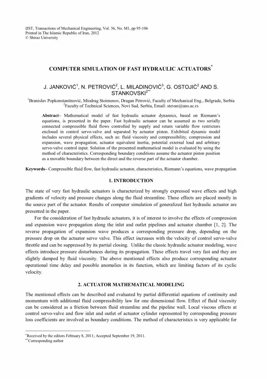
Complete actuator system (points B through I), connected into the hydraulic system into points O (supply) and K (return) to the power source hydraulic system, is presented in Fig. 1b. Static pressures in supply and return pipelines are presented as ps and p0, respectively.

(a) (b)

Fig. 1. Actuator system

Full problem formulation includes equations of characteristics with corresponding boundary and initial conditions for each of the assumed system sub-domains [3]. These domains correspond to the inlet and outlet pipelines, supply and return fluid flow sections between the control servo-valve and the actuator piston. Wave effects of return flow are very small.

As a boundary condition at point O can be assumed as the nominal supply pressure of hydraulic system, the nominal supply pressure can be assumed as the boundary condition at point O. In points A and B corresponding boundary conditions are defined as flow continuity between A and B, and pressure loss between A and B is caused by control inlet servo-valve throttle. In points C and D boundary conditions are the same type as for the points A and B with the only difference in pressure loss caused by fluid viscous

J. Janković et al.


98

effects at cylinder flow inlet and outlet. At point E the boundary conditions are defined as static pressure and piston velocity equal to the fluid velocity. In points I and J corresponding boundary conditions are defined as flow continuity between I and J, and pressure loss between I and J is caused by outlet control servo-valve throttle. In points G and H the boundary conditions are the same type as for the points C and D with the only difference in pressure loss caused by fluid viscous effects at cylinder flow outlet. At point F boundary conditions of static pressure and piston velocity equal to the fluid velocity are defined, in addition to piston equilibrium ordinary differential equation. In point K boundary conditions are assumed as zero static pressure of return fluid flow.

Initial conditions are defined at each of the domains. Initial conditions of fluid flow are assumed to be zero fluid velocity. Initial conditions of fluid static pressure are assumed to be supply static pressure (O-A) and cylinder static supply pressure (B-E and F-I). Initial and boundary conditions compatibility is completed for the exhibited system model.

4. BOUNDARY CONDITIONS OF COMPLETE ACTUATOR SYSTEM Boundary conditions of complete actuator system are defined at the following seven points: point of fluid flow separation to the actuator, input control valve, fluid inlet into actuator chamber, movable piston, the fluid outlet from actuator chamber, output control servo-valve and point of connection to the return pipeline. Corresponding boundary conditions are defined in the form of continuity and Bernoulli equations or piston momentum equation in addition to the pressure and velocity conditions [5]. Left boundaries are determined with Q-characteristics, and right ones by P-characteristics. At the boundaries A&B through I&J corresponding values of μ and u must be determined by interpolation. Certain numerical integration methods for determining the corresponding pressure value on the movable piston surface must be applied at points E&F. a) Boundary conditions of inlet and outlet control servo-valve

Boundary conditions of fluid flow are given by the following algebraic non-linear equations on the changeable restrictor:

Qppdx NMr )(2

0 (8.1)

NNNMMM uAuAQ 0

(8.2) where indexes M and N denote the corresponding points on both sides of the restrictor. It is of interest to establish the relation between derivatives of Eqs. (8), because it defines the corresponding pressure derivative along the streamline as a result of the rising hydraulic impact. By taking temporal partial derivative Eqs. (8.1), we get:

tuA

tp

tp

ppdx

ppt

xd

tQ

NM

NM

r

NMr

)(2

)(2

0

0 (9)

By substituting relations (7.1) into relation (9) and maximizing the left side of relation (9), we can give the following partial differential relation:

NMNM

NMr

xpApp

txd

,0,0)(2

(10)



99

Partial differential relation (10) shows the relationship between the input velocity of the servo-valve throttle and the pressure derivative along the fluid streamline. This relation proves that the existence of the servo-valve throttle changes cause corresponding local changes of pressure, or produce the corresponding compression and expansion waves.

Instead of this formulation, we can use the following equivalent Bernoulli’s equation with the additional equation of continuity in the form:

NNNMMM

NN

rNN

N

N

NM

M

rMM

M

M

M

uAuA

uuxd

Apuuxd

Ap

)sgn(

2)sgn(

2

2222

(11)

b) Boundary conditions on the fluid flow inlet and outlet of actuator chamber

Previous relations for the actuator servo-valve can be applied for determination of the mentioned boundary conditions (11) in the following form of fixed restrictor:

NNMM

MM

N

MMN

NM

M

NN

M

NNN

NM

M

NN

MM

N

N

M

M

uAuA

uuAAuuuuu

uuAAuuuuu

uuuupp

)sgn(2

1))(sgn()sgn(2

)sgn(2

)sgn(2

1))(sgn()sgn(2

)sgn(2

)sgn(2

)sgn(2

22

0

22

0

22

0

22

0

22

0

(12)

where η0 is corresponding coefficient of total pressure losses in the inlet and outlet points of the streamline. c) Boundary conditions of actuator piston

Equations of piston equilibrium are given in the form:

NMk

kk

kk

k

kk

k

aNM

uuu

uAmu

Ax

Akpp

.

(13)

where

ak - aero dynamical stiffness, kA - piston surface, k -coefficient of viscous dumping, km - piston mass

d) Boundary conditions at the end points

Boundary conditions in these points are caused by the performances and behavior of the hydraulic system power pump and its connection with the relief valve. This means that corresponding boundary conditions can be defined in an alternative form as follows:

maxmax

max0

max

maxmax0

;);(

);(0;

p

p

p

ppVpptu

u

VutpVup

p (14)

J. Janković et al.


100

The boundary conditions at the point O are defined in the form:

maxmax0

maxmax0

)(;

)(0;

p

p

ptpVu

Vtupp

(15)

At the point of connection to the return pipeline, the boundary condition is:

0kp (16)

5. SIMULATION MODEL PERFORMANCES It is more convenient to present the given equations in nondimensional form by introducing the following nondimensional system of coordinates and variables:

TtcLT

pp

LxV

u

p

x

u

max

max

(17)

where Vmax is maximal possible fluid velocity along the streamline caused by the system pump, pmax is maximal possible fluid nominal static pressure and L is total length of the assumed streamline.

Computer package for the fast cyclic hydraulic actuator simulation contains the mathematical description of all important physical effects existing in the transient state of its motion [6, 7]. As explained previously, significant values of velocity and pressure gradients caused by fast servo-valve throttle wave effects expressed with the mentioned travelling gradients and the effects of wave reflection are of interest. It is well known that actual hydraulic cyclic actuators have the frequency range upon 100 Hz in correlation with the conventional ones, whose frequency is limited to 10 to 20 Hz. The presented results of computer simulation illustrate that wave effects have influence on the faster types of actuators. If we consider some hypothetical types of compact actuators whose frequency range is significantly greater than 100 Hz, we must include the full influence of wave effects. This produces completely different behavior in compression with actual types of fast cyclic hydraulic actuators. The main difference is that wave reflection and corresponding velocity and pressure gradients have the same order of magnitude as the frequency range of the actuator input servo-valve control throttle. Quasi-static system behavior is practically deformed in this case and wave propagation effects take a main role. As is shown in the paper and attached references, inclusion of wave effects makes the mathematical model more complicated because it is described by partial differential equations instead of by ordinary ones. Well-known boundary conditions will change the conventional models to a very difficult procedure. The interaction of two-connected boundaries with coupled parameters on both boundaries sides which can be moved with arbitrary velocity is an example of these modifications.

More simplified one-sided actuator approximation is presented in the paper [1]. Its outlet servo-valve part and reverse chamber were neglected by assuming quasi-static fluid flow with zero static pressure and constant fluid velocity along the stream-line. This approximation enables more simplified problem



101

formulation because the effects of time delay of characteristics between inlet and outlet actuator servo-valve parts are not present. In addition, we have only one point of control input. Although this approximation can be of interest, the given results are not of high quality. This fact is compensated by the relatively simplified procedure of its feedback analysis and corresponding active control synthesis [8]. For the complete system model formulation, all of the mentioned problems, such as reverse fluid flow in the return actuator subspace must be solved efficiently.

Density of nodal point distribution along the stream-line and along the simulation time depends on maximal velocity and pressure gradients. This fact can require more computations, which usually increase cumulative computational errors. For usual actuator geometry, 200 points along the stream-line gives about 130.000 iterations per second, or a total of 26 million nodal points and corresponding calculations. In addition, each step of computation has the same number of medium nodal points. Assuming the iterative procedure of nodal points calculation, we have to build a very strict procedure without any interpolations and extrapolations, except where they cannot be overlaid. Method accuracy is very high because maximal errors of velocity and pressure distribution are very small. The corresponding differences between the results of one- and two-step iterative procedures for the case of 100 Hz actuator are less than 1x10-4 of the maximal values. Corresponding results are shown in Figs. 3a and 3b.

Time delay of characteristics is shown in the diagrams in Figs. 5d to 5f. If the changes of tangent coefficients of characteristics are less than 2.5%, the corresponding time delay is of the same magnitude value or less. If the system discretization assumes a step of 0.5% of the unit time ratio, the corresponding time delay compensation can be evaluated with no more than five iterations, which is a very convenient result. But corresponding inversion of the actuator connecting points produces more difficulties, which are explained in the following Figs. 2a to 2d.

Inversion of fluid flow between direct and reverse actuator modes is assumed as inversion of points of the inlet and outlet servo-valve parts. Any other assumption of inverting the points position is not correct, because it can produce non-existing high pressure and velocity gradients in reality. Compensation of characteristics time delay needs an iterative procedure for calculating the corresponding parameters in its domain between the points of the inlet and outlet servo-valve zero throttles.

6. DISCUSSION OF GIVEN RESULTS

In accordance with the assumed non-dimensional units length ratio of total streamline length and corresponding non-dimensional time ratio step of simulation loop, the problem of numeric stability and convergence is of great interest. For equivalent time and co-ordinate step in the assumed example, whose co-ordinate discretization is equal to 0.005 of a unit, for simulation only one second of actuator activity needed approximately 1.3 x 105 non-dimensional time steps and loop execution iterations. For that very high number of iterations, numerical accuracy of calculation on the fixed and movable boundaries is critical. To solve this problem, a corresponding interpolation or extrapolation procedure was established. In order to reduce computational oscillations around ‘exact’ solution, it is more effective to corresponding point of boundary calculations at least equal to the larger corresponding point of boundary calculations at the left and right boundaries. If we assume the middle point between the points on the left and right boundaries, the numerical convergence and the corresponding time length of the simulation process are limited to 4 x103 iterations. This value is not acceptable for practical purposes. If we assume the maximum of these time values on the corresponding boundaries, the accuracy is much higher and enables a time simulation period of 1x 105 iteration loops.

J. Janković et al.


102

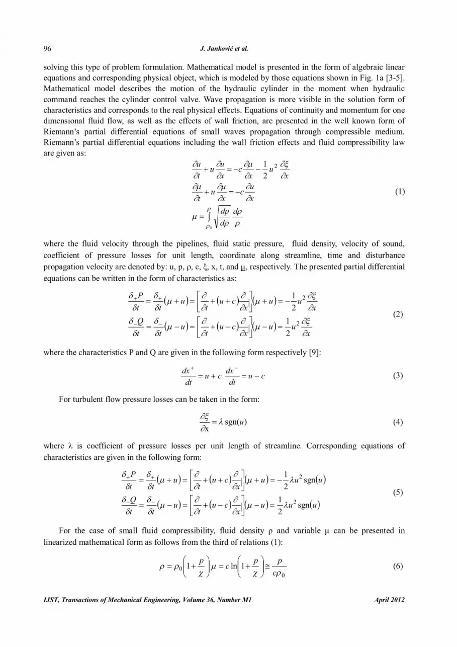
7. EXAMPLES AND GRAPHS By using the performances of the corresponding computer package actuator, simulation results can be presented in several very impressive ways. Except for 3-D diagrams that enable the presentation of each problem parameter as a 3-D surface, depending on the streamline length and time axis, it is also possible to create the animations for the distribution of corresponding parameters along the streamline axis for the assumed time sequences. In order to show all of the relevant package performances, the simulation results of some important cases of actuator and impute configuration are presented. The diagrams shown correspond to the actuator input, whose period is equal to 40 non-dimensional time units. This value corresponds to the actual actuator construction, whose frequency input range is up to 100 Hz. The 3-D results of actuator simulation are presented in Fig. 2. In Fig. 2a a non-dimensional velocity distribution is presented along the unit non-dimensional streamline and non-dimensional time domain, shown in Fig. 3d (limited from 50.570 to 50.577 time units).

a b

c d

e f

Fig. 2. 3-D results of actuator simulation

For actual types of fast cyclic actuators 1 second is equal to 650 non-dimensional time units. Six domains of streamline exist, as previously explained. The first and the last ones correspond to the source and return pipelines of the actuator. In these domains, reverse fluid flow is very small and can practically be neglected. In the middle sub-domains between the inlet and outlet servo-valve parts, velocity distribution shows that reverse motion of the actuator piston and corresponding velocity distribution along the streamline have the same order of magnitude for the positive and negative control inputs in accordance with Fig. 5a. Corresponding asymmetry of piston motion as a result of direct and reverse actuator modes,



103

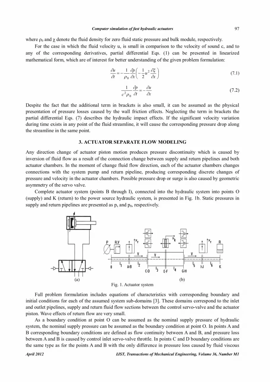
which produce asymmetric piston positions (different from zero), is presented for both piston movable boundaries in Fig. 3c. Velocity distribution for the 12 characteristic actuator cross-sections, including the movable boundaries of both sides of the actuator piston, is presented in Fig. 2c. These results are calculated and shown for each step of the simulation loops, in contrast to the diagram in Fig. 2a, which is calculated for the loops of 72 non-dimensional time simulation steps. The introduced procedure is the only one acceptable because of the package and computer memory limits. Both diagrams in Figs. 2a and 2c are calculated for two iteration steps. The corresponding difference between the one and two iteration steps procedure of the calculation of non-dimensional velocity at 12 characteristic cross-sections is presented in Fig. 2e. The error of non-dimensional velocity distribution is presented in the 3-D diagram of Fig. 3a. Corresponding maximal velocity distribution error is less than 1 x 10-4 of the non-dimensional unit velocity, or approximately 3 x 10-3of the existing velocity distribution. These results show that the iteration procedure should be accepted.

Everything shown in the Figs. 2a, 2c, 2e and 3a for non-dimensional fluid velocity distribution is presented in Figs. 2b, 2d, 2f and 3b, respectively, for non-dimensional static pressure distribution and corresponding pressure error calculations. The presented conclusions can be applied on pressure distribution without any changes.

Velocity and pressure non-dimensional distribution along the streamline at the final moment of simulation are presented in Figs. 3e and 3f, respectively. The main difference between the presented and classical actuator modeling is the nonexistence of symmetric pressure drop at the inlet and outlet servo-valve parts. Velocity distribution practically degenerates to zero.

a b

c d

e f

Fig. 3. Velocity and pressure non-dimensional distribution

J. Janković et al.


104

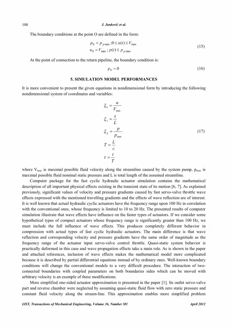
Network of characteristic points is presented in Fig. 4a, deflecting in the domain between the inlet and outlet of the actuator chamber by the influence of piston motion. Deflection of the presented mash is practically neglected in accordance with piston motion (Fig. 3c), which is also shown in Fig. 4b for all streamline domains. Several sequences of non-dimensional velocity distribution in the initial transient phase of the actuator function are shown in Figs. 4c and 4e. Corresponding non-dimensional pressure distribution is shown in the Figs. 4d and 4f, respectively. A significant difference with quasi-static actuator behavior as a result of classic modeling approach is visible in the mentioned diagrams.

a b

c d

e f

Fig. 4. Sequences of non-dimensional velocity distribution The diagram of assumed control servo-valve input throttle law for the actuator example presented, whose results are shown in all of the exhibited diagrams is presented in Fig. 4a. Fluid non-dimensional velocity distribution during time for 12 characteristic cross-sections for each of the time-step calculation loops is presented in Fig. 5b. On the other diagrams in Fig. 5, non-dimensional pressure distribution (Fig. 5c) and non-dimensional velocity distribution for different time simulation periods (Figs. 5d, 5e and 5f) are presented. Three previously mentioned diagrams are short-time sequences, because they explicitly show the wave travelling effects along the streamline during the time in the transient actuator state. If the simulation period increases, then none of the changes in step velocity becomes visibly smaller, because the velocity values also increase. Velocity step distribution is also visible in Fig. 5b. These diagrams show that the same computational procedure (and computer package) is used for the short and long time period simulations, with no accuracy problems.



105

a b

c d

e f

Fig. 5. Sequences of non-dimensional pressure distribution

8. CONCLUSION Computer simulation of fast cyclic hydraulic servo-actuator is a very effective tool in the procedure of actuator synthesis. The effect of fluid compressibility introduces additional wave propagation problems that can be solved by some numerical methods. For simulation purposes, the method of characteristics for system modeling is recommended. The presented results of actuator simulation prove that the exhibited system model and corresponding computer package enable its simulation for any arbitrary actuator configuration and states of operation.

REFERENCES 1. Zarei-nia, K., Goharrizi, A. Y., Sepehri, N. & Fung, W. (2009). Experimental evaluation of bilateral control

schemes applied to hydraulic actuators: A comparative study. Transactions of the Canadian Society for Mechanical Engineering, Vol. 33, pp. 377-398.

2. Xu, Z., Xiaowu, K. & Wei, S. (2008). Analysis and simulation of fast electro-hydraulic actuator. Mechanical & Electrical Engineering Magazine, Zhejiang University, Hangzhou, China, DOI: CNKI: SUN:JDGC.0.

3. Gomis-Bellmunt, O., Campanile, F., Galceran-Arellano, S., Montesinos-Miracle, D. & Rull-Duran, J. (2008). Hydraulic actuator modeling for optimization of mechatronic and adaptronic systems. Mechatronics, Vol. 18, pp. 634-640.

J. Janković et al.


106

4. Tadi Beni, Y., Movahhedy, M. R. & Farrahi, G. H. (2010). A complete treatment of thermo-mechanical ALE analysis; Part I: Formulation. Iranian Journal of Science & Technology, Transaction B: Engineering, Vol. 34, pp. 135-148.

5. Nayebi, A. (2010). Analysis of Bree’s cylinder with nonlinear kinematic hardening behaviour. Iranian Journal of Science & Technology, Transaction B: Engineering. Vol. 34, pp 487-498.

6. Tadic, B., Vukelic, D. J., Hodolic, J., Mitrovic S. & Eric, M. (2011). Conservative-force-controlled feed drive system for down milling. Strojniski Vestnik-Journal of Mechanical Engineering, Vol. 57, pp. 425-439.

7. Jankovic, L. (1996). Computer analysis and simulation of transient state and pressure recovering in fast cyclic hydraulic actuators. Proceedings of ICAS, ICAS-96-1.4.3, Sorrento.

8. Karpenko, M. & Sepehri, N. (2010). On quantitative feedback design for robust position control of hydraulic actuators. Control Engineering Practice, Vol. 18, pp. 289-299.

9. Novak, P., Guinot, V., Jeffrey, & Reeve, D.E. (2010). Hydraulic Modelling-an introduction. Spon press, USA & Canada, ISBN 0-203-86162-0.

computer simulation of fast hydraulic actuators

Documents