water

Article

Evaluating Curb Inlet Efficiency for Urban Drainageand Road Bioretention Facilities

Xiaoning Li 1,2, Xing Fang 1,3,* , Gang Chen 2 , Yongwei Gong 3, Jianlong Wang 3 and Junqi Li 3

1 Department of Civil Engineering, Auburn University, Auburn, AL 36849-5337, USA; xzl0055@auburn.edu2 College of Hydrology and Water Resources, Hohai University, No. 1 Xikang Road, Nanjing 210098, China;

gangchen@hhu.edu.cn3 Key Laboratory of Urban Stormwater System and Water Environment, Ministry of Education, Beijing

University of Civil Engineering and Architecture, Beijing 100044, China; gongyongwei@bucea.edu.cn (Y.G.);wjl_xt@163.com (J.W.); lijunqi@bucea.edu.cn (J.L.)

* Correspondence: xing.fang@auburn.edu; Tel.: +1-334-844-8778; Fax: +1-334-844-6290

Received: 4 April 2019; Accepted: 17 April 2019; Published: 23 April 2019�����������������

Abstract: An updated two-dimensional flow simulation program, FullSWOF-ZG, which fully (Full)solves shallow water (SW) equations for overland flow (OF) and includes submodules modelinginfiltration by zones (Z) and flow interception by grate-inlet (G), was tested with 20 locally depressedcurb inlets to validate the inlet efficiency (Eci), and with 80 undepressed curb inlets to validate the inletlengths (LT) for 100% interception. Previous curb inlet equations were based on certain theoreticalapproximations and limited experimental data. In this study, 1000 road-curb inlet modeling casesfrom the combinations of 10 longitudinal slopes (S0, 0.1–1%), 10 cross slopes (Sx, 1.5–6%), and10 upstream inflows (Qin, 6–24 L/s) were established and modeled to determine LT. The second1000 modeling cases with the same 10 S0 and 10 Sx and 10 curb inlet lengths (Lci, 0.15–1.5 m) wereestablished to determine Eci. The LT and Eci regression equations were developed as a function ofinput parameters (S0, Sx, and Qin) and Lci/LT with the multiple linear regression method, respectively.Newly developed regression equations were applied to 10,000 inlet design cases (10 S0, 10 Sx, 10 Qin,and 10 Lci combinations) and comprehensively compared with three equations in previous studies.The 100% intercepted gutter flow (Qg100) equations were derived, and over-prediction of Qg100 fromprevious methods was strongly correlated to smaller S0. Newly developed equations gave moreaccurate estimations of LT and Eci over a wide range of input parameters. These equations can beapplied to designing urban drainage and road bioretention facilities, since they were developedusing a large number of simulation runs with diverse input parameters, but previous methods oftenoverpredict the gutter flow of total interception when the longitudinal slope S0 is small.

Keywords: curb inlet; overland flow; two-dimensional simulation; bioretention; intercepted flow;inlet efficiency

1. Introduction

The urban drainage system is designed and built to effectively convey the rainfall runoff out of theurban area to prevent inundation and local flooding [1], which can cause property damage and affecttraffic and human safety. Curb inlets effectively intercept surface runoff into underground drainagepipes or bioretention facilities. As an important and typical practice, road bioretention facilities, whichcombine green/gray infrastructures to facilitate road runoff control through infiltration and storage,remove certain contaminants and sediments, and decrease roads’ local flood inundation risk, arewidely used in the pilot Sponge City construction in China [2] and all over the world. Li et al. [3]found that the curb inlet could be the bottleneck of road bioretention facilities that impedes the runoff

Water 2019, 11, 851; doi:10.3390/w11040851 www.mdpi.com/journal/water

Water 2019, 11, 851 2 of 18

generated from the road flowing into the bioretention to infiltrate, detain (pond), and improve thestormwater quality. Tu and Traver [4] found that the perforated distribution pipe could be an uncertainfactor on road bioretention performance. Stoolmiller et al. [5] surveyed curb inlets for road bioretentionfacilities in Philadelphia, and the curb inlet opening ranged from 0.15 m (6 inches) to 1.52 m (5 ft).Some of these inlets seem to have been designed based on the landscape and from a safety perspective,instead of hydraulic performance considering inlet interception efficiency.

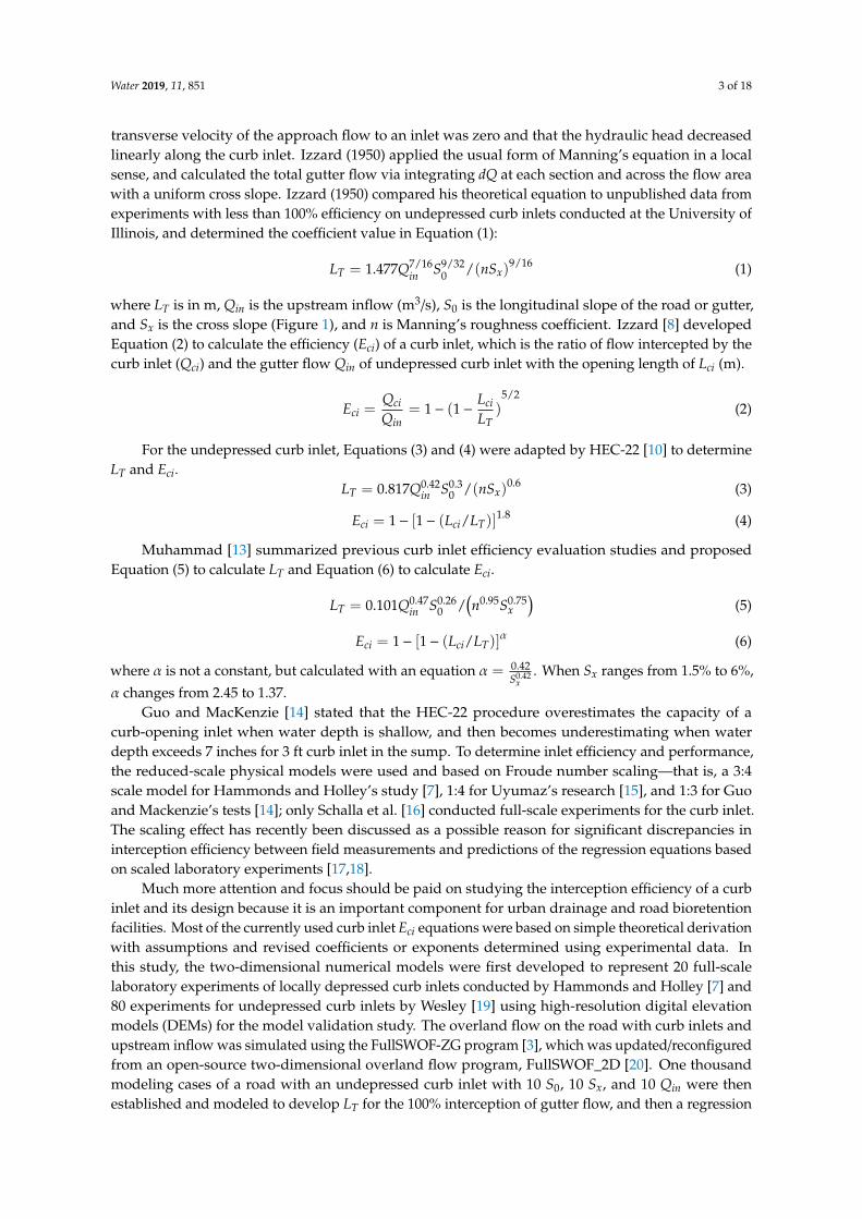
There are three types of curb inlets commonly used along urban streets. The undepressed curbinlet has one cross slope for the road, gutter, and curb inlet. The continuously depressed curb inletis placed in the gutter of a street with a steeper cross slope than the road cross slope [6]. The locallydepressed curb inlet has adjacent depressions in the gutter before and/or after the inlet for effectiveflow interception—for example, type C and type D curb inlets, designed and constructed by the TexasDepartment of Transportation (TxDOT) [7], have a 5 to 15 ft locally depressed curb opening, and 5 fttransition sections at the upstream and downstream of the opening (Figure 1). The upstream transitionsection changes elevation gradually from the undepressed section into fully depressed inlet sectionover the 1.52 m (5 ft) length, and the downstream transition section gradually decreases the localdepression (Figure 1).

Water 2019, 11, x 2 of 18

impedes the runoff generated from the road flowing into the bioretention to infiltrate, detain (pond),

and improve the stormwater quality. Tu and Traver [4] found that the perforated distribution pipe

could be an uncertain factor on road bioretention performance. Stoolmiller et al. [5] surveyed curb

inlets for road bioretention facilities in Philadelphia, and the curb inlet opening ranged from 0.15 m

(6 inches) to 1.52 m (5 ft). Some of these inlets seem to have been designed based on the landscape

and from a safety perspective, instead of hydraulic performance considering inlet interception

efficiency.

There are three types of curb inlets commonly used along urban streets. The undepressed curb

inlet has one cross slope for the road, gutter, and curb inlet. The continuously depressed curb inlet is

placed in the gutter of a street with a steeper cross slope than the road cross slope [6]. The locally

depressed curb inlet has adjacent depressions in the gutter before and/or after the inlet for effective

flow interception—for example, type C and type D curb inlets, designed and constructed by the Texas

Department of Transportation (TxDOT) [7], have a 5 to 15 ft locally depressed curb opening, and 5 ft

transition sections at the upstream and downstream of the opening (Figure 1). The upstream

transition section changes elevation gradually from the undepressed section into fully depressed inlet

section over the 1.52 m (5 ft) length, and the downstream transition section gradually decreases the

local depression (Figure 1).

Figure 1. (a) Layout of the Type D curb inlet evaluation experiment, and (b) digital elevation model

(DEM) of case D01 with S0 = 0.004 and Sx = 0.0208.

The hydraulic performance of curb inlets for roadway drainage has been studied for more than

60 years, which was reviewed and summarized by Izzard [8], Li [9], and presently systematically

documented in the Hydraulic Engineering Circular No. 22 (HEC-22) by Brown et al. [10]. In 1979, the

Federal Highway Administration [11] first published a technical guide for the design of urban

highway drainage, and then updated it in 1984 into a HEC-12 entitled “Drainage of Highway

Pavement’’ [12]. HEC-12 summarizes a semi-theoretical method developed for estimating street

hydraulic capacities and procedures for sizing street inlets. The most recent HEC-22 [10] was

published and widely used in the USA, and refined the design procedures stated in HEC-12.

Izzard [8] developed equations to calculate the normal depth of gutter flow and the curb opening

length (LT) (Equation (1)) required to intercept 100% of the gutter flow. Izzard [8] assumed that the

Figure 1. (a) Layout of the Type D curb inlet evaluation experiment, and (b) digital elevation model(DEM) of case D01 with S0 = 0.004 and Sx = 0.0208.

The hydraulic performance of curb inlets for roadway drainage has been studied for more than60 years, which was reviewed and summarized by Izzard [8], Li [9], and presently systematicallydocumented in the Hydraulic Engineering Circular No. 22 (HEC-22) by Brown et al. [10]. In 1979, theFederal Highway Administration [11] first published a technical guide for the design of urban highwaydrainage, and then updated it in 1984 into a HEC-12 entitled “Drainage of Highway Pavement” [12].HEC-12 summarizes a semi-theoretical method developed for estimating street hydraulic capacitiesand procedures for sizing street inlets. The most recent HEC-22 [10] was published and widely used inthe USA, and refined the design procedures stated in HEC-12.

Izzard [8] developed equations to calculate the normal depth of gutter flow and the curb openinglength (LT) (Equation (1)) required to intercept 100% of the gutter flow. Izzard [8] assumed that the

Water 2019, 11, 851 3 of 18

transverse velocity of the approach flow to an inlet was zero and that the hydraulic head decreasedlinearly along the curb inlet. Izzard (1950) applied the usual form of Manning’s equation in a localsense, and calculated the total gutter flow via integrating dQ at each section and across the flow areawith a uniform cross slope. Izzard (1950) compared his theoretical equation to unpublished data fromexperiments with less than 100% efficiency on undepressed curb inlets conducted at the University ofIllinois, and determined the coefficient value in Equation (1):

LT = 1.477Q7/16in S9/32

0 /(nSx)9/16 (1)

where LT is in m, Qin is the upstream inflow (m3/s), S0 is the longitudinal slope of the road or gutter,and Sx is the cross slope (Figure 1), and n is Manning’s roughness coefficient. Izzard [8] developedEquation (2) to calculate the efficiency (Eci) of a curb inlet, which is the ratio of flow intercepted by thecurb inlet (Qci) and the gutter flow Qin of undepressed curb inlet with the opening length of Lci (m).

Eci =Qci

Qin= 1− (1−

LciLT

)5/2

(2)

For the undepressed curb inlet, Equations (3) and (4) were adapted by HEC-22 [10] to determineLT and Eci.

LT = 0.817Q0.42in S0.3

0 /(nSx)0.6 (3)

Eci = 1− [1− (Lci/LT)]1.8 (4)

Muhammad [13] summarized previous curb inlet efficiency evaluation studies and proposedEquation (5) to calculate LT and Equation (6) to calculate Eci.

LT = 0.101Q0.47in S0.26

0 /(n0.95S0.75

x

)(5)

Eci = 1− [1− (Lci/LT)]α (6)

where α is not a constant, but calculated with an equation α = 0.42S0.42

x. When Sx ranges from 1.5% to 6%,

α changes from 2.45 to 1.37.Guo and MacKenzie [14] stated that the HEC-22 procedure overestimates the capacity of a

curb-opening inlet when water depth is shallow, and then becomes underestimating when waterdepth exceeds 7 inches for 3 ft curb inlet in the sump. To determine inlet efficiency and performance,the reduced-scale physical models were used and based on Froude number scaling—that is, a 3:4scale model for Hammonds and Holley’s study [7], 1:4 for Uyumaz’s research [15], and 1:3 for Guoand Mackenzie’s tests [14]; only Schalla et al. [16] conducted full-scale experiments for the curb inlet.The scaling effect has recently been discussed as a possible reason for significant discrepancies ininterception efficiency between field measurements and predictions of the regression equations basedon scaled laboratory experiments [17,18].

Much more attention and focus should be paid on studying the interception efficiency of a curbinlet and its design because it is an important component for urban drainage and road bioretentionfacilities. Most of the currently used curb inlet Eci equations were based on simple theoretical derivationwith assumptions and revised coefficients or exponents determined using experimental data. Inthis study, the two-dimensional numerical models were first developed to represent 20 full-scalelaboratory experiments of locally depressed curb inlets conducted by Hammonds and Holley [7] and80 experiments for undepressed curb inlets by Wesley [19] using high-resolution digital elevationmodels (DEMs) for the model validation study. The overland flow on the road with curb inlets andupstream inflow was simulated using the FullSWOF-ZG program [3], which was updated/reconfiguredfrom an open-source two-dimensional overland flow program, FullSWOF_2D [20]. One thousandmodeling cases of a road with an undepressed curb inlet with 10 S0, 10 Sx, and 10 Qin were thenestablished and modeled to develop LT for the 100% interception of gutter flow, and then a regression

Water 2019, 11, 851 4 of 18

equation of LT as a function of input parameters was developed by the multiple linear regressionmethod. The second 1000 modeling cases of the road with 10 S0, 10 Sx, and 10 curb inlet lengths Lci wereestablished and simulated to determine Eci of different Lci, and a regression equation of Eci as a functionof Lci/LT was also developed. The simulation results of LT and Eci were discussed and comprehensivelycompared with calculated/predicted results from HEC-22 [10], Izzard [8], and Muhamad [13]. In thisstudy, the height of the opening of the curb inlets was not directly considered when a two-dimensionalmodel was used. Only under severe flood situations was the height of the opening found to play a roleon flow interception and inlet efficiency.

2. Materials and Methods

Fang et al. [21] used a three-dimensional computational fluid dynamics (CFD) software, Flow-3D,to develop the numerical models simulating unsteady, free-surface, shallow flow through Type C andType D [7] curb-opening inlets. They demonstrated that an advanced CFD model could be used asa virtual laboratory to evaluate the performance of curb inlets with different geometry and inflowconditions. In this study, the two-dimensional open source FullSWOF_2D (version 1.07, DieudonnéLaboratory J.A., Polytech Nice Sophia, Nice, France) [20] program was updated to simulate the complexflow through an inlet to determine the inlet-opening length LT of 100% (total) interception, and theefficiency Eci of an undepressed curb inlet.

The FullSWOF_2D program fully solves shallow-water equations (SWEs) [20], depth-integratingthe Navier–Stokes equations [22] on a structured mesh (square cells) in two-dimensional domainsusing the finite volume method [23], and is programmed using C++ to fully describe the rainfall-runoff

and flow distribution progress on the surface [24]. As a Saint-Venant system [22], the SWEs model iswidely used to simulate the incompressible Navier–Stokes flow occurring in rivers, channels, ocean,and land surfaces [25]. It is derived with two assumptions: the water depth is small with respect to thehorizontal (x, y) dimensions, and the pressure of the fluid is hydrostatic (∂p/∂z = −g), which meansthe pressure field could be calculated with simple integration along the vertical (z) direction [26]. Awell-balanced numerical scheme was adapted to guarantee the positivity of water height and thepreservation of steady states for specific hydrological features, such as during wet–dry transitionsand tiny water depth [27]. Different boundary conditions, friction laws, and numerical schemes weredeveloped, which make the program a very powerful overland flow simulation software [20].

The FullSWOF_2D program, which applies the uniform rainfall and infiltration parameters tothe whole simulation domain, was revised by Li et al. [3] to include 2D plane zones (Z) with differentrainfall and infiltration parameters and a 2D-1D grate-inlet (G) drainage module. Therefore, theupdated FullSWOF-ZG program can simulate impervious and pervious surfaces (different infiltrationparameters/capabilities in different zones) in the road bioretention domain simultaneously underrainfall events. The 2D-1D grate-inlet drainage submodule enables the program to simulate the 2Doverland runoff flowing into a grate inlet, and then to a 1D underground drainage pipe using the weirequation [28]. In Li’s study [3], the FullSWOF-ZG was used to evaluate the performance of a roadbioretention facility and explore/understand key parameters of continuous road bioretention design. Itwas found that the curb inlet becomes the bottleneck of the road bioretention strip system that couldimpede the runoff flowing into the bioretention strip for detention and infiltration to improve thestormwater quality [3].

2.1. FullSWOF-ZG Validation Cases

For the reduced-scale and full-scale laboratory experiments, the curb inlet efficiency was calculatedwith flow intercepted by the curb inlet divided by the total upstream inflow, which did not consider therainfall-runoff generation and concentration process. It was not meant to understand the performanceof the curb inlet under a rainfall event, but to provide the information for engineering design of thecurb inlet as a function of upstream inflow. Inflows with different magnitudes and spreads for curbinlets include runoff from upstream and surrounding lands and runoff produced from the roadway.

Water 2019, 11, 851 5 of 18

Therefore, these experimental studies are valuable, and numerical model studies under the sameexperimental conditions were used to validate the FullSWOF-ZG model to see how well the modelcan predict the curb inlet efficiency. Twenty locally depressed curb inlet cases, which were tested in alaboratory by Hammonds and Holley [7], were used to validate FullSWOF-ZG for curb inlet efficiencysimulation. Eighty undepressed curb inlet cases, which were tested in a laboratory by Wesley [19],were used to validate FullSWOF-ZG for curb inlet lengths of 100% interception.

2.1.1. Modeling Cases to Validate Curb Inlet Efficiency

The FullSWOF-ZG program was previously tested and verified for overland flow on pervioussurfaces [3,29]. In a previous study [3], the FullSWOF-ZG program was tested with 20 type C curbinlet cases. The coefficient of determination (R2) of the linear relationship between the simulated andobserved curb inlet interception efficiencies was 0.94 for type C curb inlet test cases. The differencesbetween the simulated and observed interception efficiencies (∆E) ranged from −3.2% to 13.2%, withan average ± standard deviation of 3.5 ± 3.5%. In this study, FullSWOF-ZG was first tested using20 locally depressed curb inlets (type D, Figure 1), which was tested in laboratory experiments byHammonds and Holley [7]. For type D curb inlet experiments, the length and width of the simulationdomain were 15.55 m (51 ft, x-direction) and 4.57 m (15 ft, y-direction), respectively. The total openinglengths of different curb inlets were either 4.57 m (15 ft) or 7.62 m (25 ft), which included a 1.52 m(5 ft) or 4.57 m (15 ft) inlet opening and 1.52 m (5 ft) upstream and downstream transition sections(Figure 1). The total width of the curb inlet depression was 0.457 m (1.5 ft), and the depressed depthwas 0.10 m (0.33 ft) and 0.076 m (0.25 ft) at a depression width of 0.368 m (1.2 ft) for type C and type Dcurb inlets, respectively.

The simulation domain was represented by a detailed and high-resolution DEM (Figure 1b) witha cell size equal to 0.076 m (0.25 ft). The elevation of every computation cell was calculated using auser-developed MATLAB r2017a (MathWorks, Natick, MA, United States) [30] code with considerationof the road’s longitudinal slope, cross slope, locally depressed cross slope of the curb inlet, and theslopes of the inlet’s upstream and downstream transition parts. The longitudinal (x-direction) and cross(y-direction) slopes for the simulation domain are from left to right and bottom to top, respectively(Figure 1). Manning’s law in FullSWOF-ZG was used in the simulation, and the roughness coefficientdetermined for the laboratory roadway was 0.018 [7].

The imposed discharge condition in FullSWOF-ZG was chosen as the left or upstream boundarycondition of the domain. The imposed discharge for the boundary cells within the spread (T) wasapproximately assumed as the total inflow rate (Qin) divided by the number of the cells within thespread and set to be equal to 0 for other boundary cells outside of the spread. The top and right(downstream) boundary of the simulation domain was set as a Neumann condition that allows theflow to get out of the simulation domain. At the top of the simulation domain, those cells on thecurb had higher elevations to prevent the outflow. The bottom boundary of the simulation domain(Figure 1b) had the highest elevation along the y-direction, and was set as a wall boundary conditionto guarantee that the flow would not pass through the bottom boundary.

2.1.2. Modeling Cases to Simulate/Validate Curb Inlet Length of 100% Interception

Wesley [19] conducted a series of full-scale experiments to determine the 100% intercepted curbinlet lengths with different longitudinal and cross slopes for undepressed curb inlets. The experimentfacility had a triangular cross-section with the curb side being nearly vertical, and placed on acontinuous grade with no local depression on the channel bottom. The length of the curb opening wassufficient to allow for interception of all the flow from the upstream road. The experiment facility was50 ft (15.24 m) in overall length and 6 ft (1.83 m) in width. At 32 ft (9.75 m) from the upstream end, thecurb inlet opening began. This upstream length (32 ft) is sufficient for the development of a uniformflow condition. The 100% intercepted curb inlet length was then experimentally determined using theobserved distribution of water depth along the curb [19].

Water 2019, 11, 851 6 of 18

The simulation domain was represented by detailed and high-resolution DEM with a smaller cellsize equal to 0.05 ft (0.015 m), similar to Figure 1 without local depressions. The Manning’s value was0.01, which is the same as the experiment facility. For eighty experimental cases, S0 ranged from 0.005to 0.05, Sx ranged from 0.01 to 0.08, and upstream inflow Qin ranged from 0.18 L/s to 84.38 L/s, whichwere simulated to determine the 100% interception curb inlet lengths.

2.2. Modeling Cases to Evaluate 100% Interception Length and Curb Inlet Efficiency

After the FullSWOF-ZG model was validated to be able to accurately simulate flow over the curbinlet, 1000 modeling cases were selected and modeled to determine the curb inlet length LT of 100%interception under different S0, Sx, and Qin. The length and width of the simulation domain for these1000 modeling cases were 12 m (x-direction) including the 10 m road surface before the inlet and 6.7 m(y-direction, Figure 1) including a 3 m wide car lane stripe, 1.5 m wide bike lane strip, 2.1 m parkingstripe (1.5 m + 0.6 m gutter), and 0.1 m curb width. The cell size of DEMs for all 1000 cases was 0.025 m,determined by a sensitivity analysis.

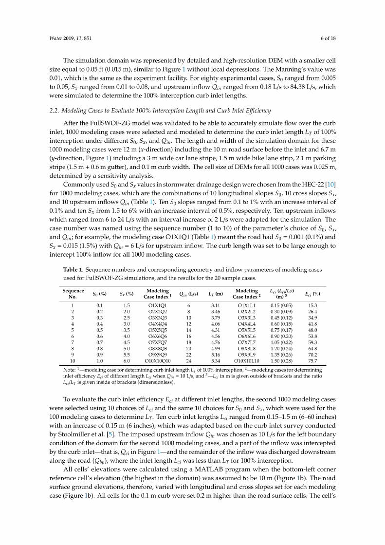
Commonly used S0 and Sx values in stormwater drainage design were chosen from the HEC-22 [10]for 1000 modeling cases, which are the combinations of 10 longitudinal slopes S0, 10 cross slopes Sx,and 10 upstream inflows Qin (Table 1). Ten S0 slopes ranged from 0.1 to 1% with an increase interval of0.1% and ten Sx from 1.5 to 6% with an increase interval of 0.5%, respectively. Ten upstream inflowswhich ranged from 6 to 24 L/s with an interval increase of 2 L/s were adapted for the simulation. Thecase number was named using the sequence number (1 to 10) of the parameter’s choice of S0, Sx,and Qin; for example, the modeling case O1X1Q1 (Table 1) meant the road had S0 = 0.001 (0.1%) andSx = 0.015 (1.5%) with Qin = 6 L/s for upstream inflow. The curb length was set to be large enough tointercept 100% inflow for all 1000 modeling cases.

Table 1. Sequence numbers and corresponding geometry and inflow parameters of modeling casesused for FullSWOF-ZG simulations, and the results for the 20 sample cases.

SequenceNo. S0 (%) Sx (%) Modeling

Case Index 1 Qin (L/s) LT (m) ModelingCase Index 2

Lci (Lci/LT)(m) 3 Eci (%)

1 0.1 1.5 O1X1Q1 6 3.11 O1X1L1 0.15 (0.05) 15.32 0.2 2.0 O2X2Q2 8 3.46 O2X2L2 0.30 (0.09) 26.43 0.3 2.5 O3X3Q3 10 3.79 O3X3L3 0.45 (0.12) 34.94 0.4 3.0 O4X4Q4 12 4.06 O4X4L4 0.60 (0.15) 41.85 0.5 3.5 O5X5Q5 14 4.31 O5X5L5 0.75 (0.17) 48.06 0.6 4.0 O6X6Q6 16 4.56 O6X6L6 0.90 (0.20) 53.87 0.7 4.5 O7X7Q7 18 4.76 O7X7L7 1.05 (0.22) 59.38 0.8 5.0 O8X8Q8 20 4.99 O8X8L8 1.20 (0.24) 64.89 0.9 5.5 O9X9Q9 22 5.16 O9X9L9 1.35 (0.26) 70.2

10 1.0 6.0 O10X10Q10 24 5.34 O10X10L10 1.50 (0.28) 75.7

Note: 1—modeling case for determining curb inlet length LT of 100% interception, 2—modeling cases for determininginlet efficiency Eci of different length Lci when Qin = 10 L/s, and 3—Lci in m is given outside of brackets and the ratioLci/LT is given inside of brackets (dimensionless).

To evaluate the curb inlet efficiency Eci at different inlet lengths, the second 1000 modeling caseswere selected using 10 choices of Lci and the same 10 choices for S0 and Sx, which were used for the100 modeling cases to determine LT. Ten curb inlet lengths Lci ranged from 0.15–1.5 m (6–60 inches)with an increase of 0.15 m (6 inches), which was adapted based on the curb inlet survey conductedby Stoolmiller et al. [5]. The imposed upstream inflow Qin was chosen as 10 L/s for the left boundarycondition of the domain for the second 1000 modeling cases, and a part of the inflow was interceptedby the curb inlet—that is, Qci in Figure 1—and the remainder of the inflow was discharged downstreamalong the road (Qbp), where the inlet length Lci was less than LT for 100% interception.

All cells’ elevations were calculated using a MATLAB program when the bottom-left cornerreference cell’s elevation (the highest in the domain) was assumed to be 10 m (Figure 1b). The roadsurface ground elevations, therefore, varied with longitudinal and cross slopes set for each modelingcase (Figure 1b). All cells for the 0.1 m curb were set 0.2 m higher than the road surface cells. The cell’s

Water 2019, 11, 851 7 of 18

elevations inside the curb inlet cells were calculated using the same cross slope of the road surface,which helps and allows the runoff to flow out the road surface. The total simulation duration was 120 s(1.5 min) for reaching an equilibrium condition to determine Eci.

3. Results and Discussion

3.1. FullSWOF-ZG Validation Results of Curb Inlet Efficiency

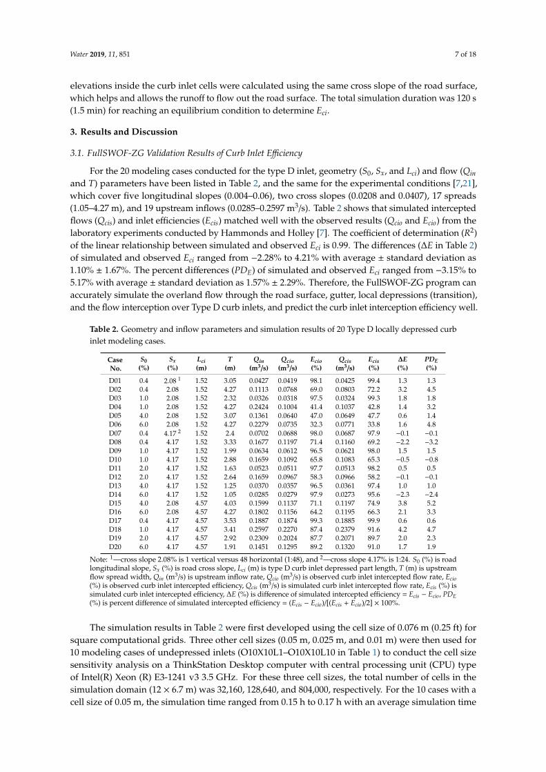
For the 20 modeling cases conducted for the type D inlet, geometry (S0, Sx, and Lci) and flow (Qinand T) parameters have been listed in Table 2, and the same for the experimental conditions [7,21],which cover five longitudinal slopes (0.004–0.06), two cross slopes (0.0208 and 0.0407), 17 spreads(1.05–4.27 m), and 19 upstream inflows (0.0285–0.2597 m3/s). Table 2 shows that simulated interceptedflows (Qcis) and inlet efficiencies (Ecis) matched well with the observed results (Qcio and Ecio) from thelaboratory experiments conducted by Hammonds and Holley [7]. The coefficient of determination (R2)of the linear relationship between simulated and observed Eci is 0.99. The differences (∆E in Table 2)of simulated and observed Eci ranged from −2.28% to 4.21% with average ± standard deviation as1.10% ± 1.67%. The percent differences (PDE) of simulated and observed Eci ranged from −3.15% to5.17% with average ± standard deviation as 1.57% ± 2.29%. Therefore, the FullSWOF-ZG program canaccurately simulate the overland flow through the road surface, gutter, local depressions (transition),and the flow interception over Type D curb inlets, and predict the curb inlet interception efficiency well.

Table 2. Geometry and inflow parameters and simulation results of 20 Type D locally depressed curbinlet modeling cases.

CaseNo.

S0 Sx Lci T Qin Qcio Ecio Qcis Ecis ∆E PDE(%) (%) (m) (m) (m3/s) (m3/s) (%) (m3/s) (%) (%) (%)

D01 0.4 2.08 1 1.52 3.05 0.0427 0.0419 98.1 0.0425 99.4 1.3 1.3D02 0.4 2.08 1.52 4.27 0.1113 0.0768 69.0 0.0803 72.2 3.2 4.5D03 1.0 2.08 1.52 2.32 0.0326 0.0318 97.5 0.0324 99.3 1.8 1.8D04 1.0 2.08 1.52 4.27 0.2424 0.1004 41.4 0.1037 42.8 1.4 3.2D05 4.0 2.08 1.52 3.07 0.1361 0.0640 47.0 0.0649 47.7 0.6 1.4D06 6.0 2.08 1.52 4.27 0.2279 0.0735 32.3 0.0771 33.8 1.6 4.8D07 0.4 4.17 2 1.52 2.4 0.0702 0.0688 98.0 0.0687 97.9 −0.1 −0.1D08 0.4 4.17 1.52 3.33 0.1677 0.1197 71.4 0.1160 69.2 −2.2 −3.2D09 1.0 4.17 1.52 1.99 0.0634 0.0612 96.5 0.0621 98.0 1.5 1.5D10 1.0 4.17 1.52 2.88 0.1659 0.1092 65.8 0.1083 65.3 −0.5 −0.8D11 2.0 4.17 1.52 1.63 0.0523 0.0511 97.7 0.0513 98.2 0.5 0.5D12 2.0 4.17 1.52 2.64 0.1659 0.0967 58.3 0.0966 58.2 −0.1 −0.1D13 4.0 4.17 1.52 1.25 0.0370 0.0357 96.5 0.0361 97.4 1.0 1.0D14 6.0 4.17 1.52 1.05 0.0285 0.0279 97.9 0.0273 95.6 −2.3 −2.4D15 4.0 2.08 4.57 4.03 0.1599 0.1137 71.1 0.1197 74.9 3.8 5.2D16 6.0 2.08 4.57 4.27 0.1802 0.1156 64.2 0.1195 66.3 2.1 3.3D17 0.4 4.17 4.57 3.53 0.1887 0.1874 99.3 0.1885 99.9 0.6 0.6D18 1.0 4.17 4.57 3.41 0.2597 0.2270 87.4 0.2379 91.6 4.2 4.7D19 2.0 4.17 4.57 2.92 0.2309 0.2024 87.7 0.2071 89.7 2.0 2.3D20 6.0 4.17 4.57 1.91 0.1451 0.1295 89.2 0.1320 91.0 1.7 1.9

Note: 1—cross slope 2.08% is 1 vertical versus 48 horizontal (1:48), and 2—cross slope 4.17% is 1:24. S0 (%) is roadlongitudinal slope, Sx (%) is road cross slope, Lci (m) is type D curb inlet depressed part length, T (m) is upstreamflow spread width, Qin (m3/s) is upstream inflow rate, Qcio (m3/s) is observed curb inlet intercepted flow rate, Ecio(%) is observed curb inlet intercepted efficiency, Qcis (m3/s) is simulated curb inlet intercepted flow rate, Ecis (%) issimulated curb inlet intercepted efficiency, ∆E (%) is difference of simulated intercepted efficiency = Ecis − Ecio, PDE(%) is percent difference of simulated intercepted efficiency = (Ecis − Ecio)/[(Ecis + Ecio)/2] × 100%.

The simulation results in Table 2 were first developed using the cell size of 0.076 m (0.25 ft) forsquare computational grids. Three other cell sizes (0.05 m, 0.025 m, and 0.01 m) were then used for10 modeling cases of undepressed inlets (O10X10L1–O10X10L10 in Table 1) to conduct the cell sizesensitivity analysis on a ThinkStation Desktop computer with central processing unit (CPU) typeof Intel(R) Xeon (R) E3-1241 v3 3.5 GHz. For these three cell sizes, the total number of cells in thesimulation domain (12 × 6.7 m) was 32,160, 128,640, and 804,000, respectively. For the 10 cases with acell size of 0.05 m, the simulation time ranged from 0.15 h to 0.17 h with an average simulation time

Water 2019, 11, 851 8 of 18

equal to 0.15 h. For the 10 cases with a cell size of 0.025 m, the simulation time ranged from 1.23 hto 1.43 h with an average simulation time equal to 1.27 h. For the 10 cases with a cell size of 0.01 m,the simulation time ranged from 26.3 h to 26.4 h. The cell size of 0.025 m (~1 inch) was chosen as thesimulation cell size for simulations of all other modeling cases in this study based on the balance of themodel accuracy in predicting Qci and Eci and the simulation time for the 10 test cases above.

3.2. Validation Results of 100% Intercepted Curb Inlet Length

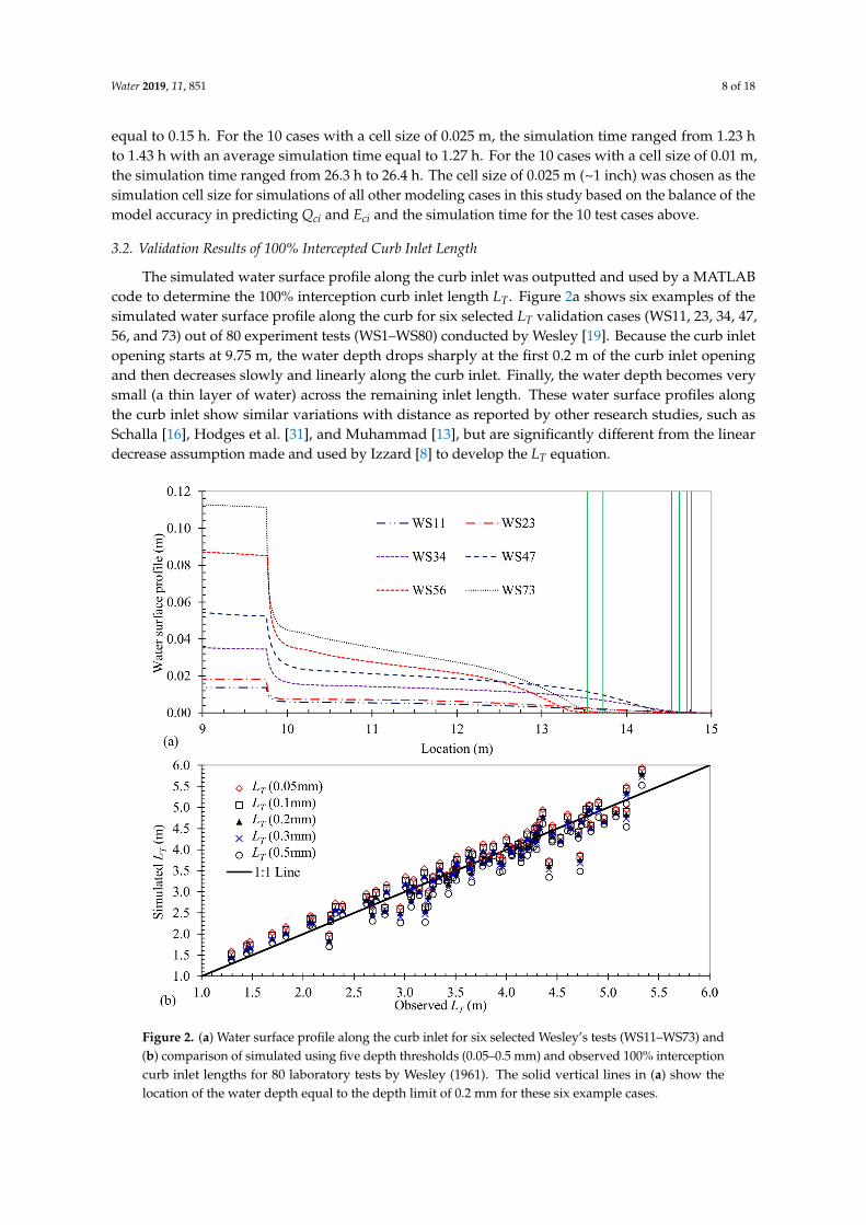
The simulated water surface profile along the curb inlet was outputted and used by a MATLABcode to determine the 100% interception curb inlet length LT. Figure 2a shows six examples of thesimulated water surface profile along the curb for six selected LT validation cases (WS11, 23, 34, 47,56, and 73) out of 80 experiment tests (WS1–WS80) conducted by Wesley [19]. Because the curb inletopening starts at 9.75 m, the water depth drops sharply at the first 0.2 m of the curb inlet openingand then decreases slowly and linearly along the curb inlet. Finally, the water depth becomes verysmall (a thin layer of water) across the remaining inlet length. These water surface profiles alongthe curb inlet show similar variations with distance as reported by other research studies, such asSchalla [16], Hodges et al. [31], and Muhammad [13], but are significantly different from the lineardecrease assumption made and used by Izzard [8] to develop the LT equation.

Water 2019, 11, x 8 of 18

simulation domain (12 × 6.7 m) was 32,160, 128,640, and 804,000, respectively. For the 10 cases with a cell size of 0.05 m, the simulation time ranged from 0.15 h to 0.17 h with an average simulation time equal to 0.15 h. For the 10 cases with a cell size of 0.025 m, the simulation time ranged from 1.23 h to 1.43 h with an average simulation time equal to 1.27 h. For the 10 cases with a cell size of 0.01 m, the simulation time ranged from 26.3 h to 26.4 h. The cell size of 0.025 m (~1 inch) was chosen as the simulation cell size for simulations of all other modeling cases in this study based on the balance of the model accuracy in predicting Qci and Eci and the simulation time for the 10 test cases above.

3.2. Validation Results of 100% Intercepted Curb Inlet Length

The simulated water surface profile along the curb inlet was outputted and used by a MATLAB code to determine the 100% interception curb inlet length LT. Figure 2a shows six examples of the simulated water surface profile along the curb for six selected LT validation cases (WS11, 23, 34, 47, 56, and 73) out of 80 experiment tests (WS1–WS80) conducted by Wesley [19]. Because the curb inlet opening starts at 9.75 m, the water depth drops sharply at the first 0.2 m of the curb inlet opening and then decreases slowly and linearly along the curb inlet. Finally, the water depth becomes very small (a thin layer of water) across the remaining inlet length. These water surface profiles along the curb inlet show similar variations with distance as reported by other research studies, such as Schalla [16], Hodges et al. [31], and Muhammad [13], but are significantly different from the linear decrease assumption made and used by Izzard [8] to develop the LT equation.

Figure 2. (a) Water surface profile along the curb inlet for six selected Wesley’s tests (WS11–WS73) and (b) comparison of simulated using five depth thresholds (0.05–0.5 mm) and observed 100% interception curb inlet lengths for 80 laboratory tests by Wesley (1961). The solid vertical lines in (a) show the location of the water depth equal to the depth limit of 0.2 mm for these six example cases.

Figure 2. (a) Water surface profile along the curb inlet for six selected Wesley’s tests (WS11–WS73) and(b) comparison of simulated using five depth thresholds (0.05–0.5 mm) and observed 100% interceptioncurb inlet lengths for 80 laboratory tests by Wesley (1961). The solid vertical lines in (a) show thelocation of the water depth equal to the depth limit of 0.2 mm for these six example cases.

Water 2019, 11, 851 9 of 18

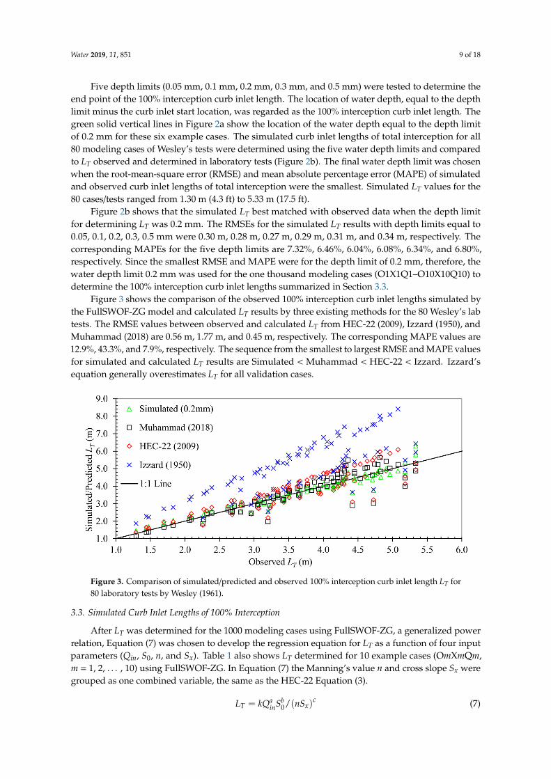
Five depth limits (0.05 mm, 0.1 mm, 0.2 mm, 0.3 mm, and 0.5 mm) were tested to determine theend point of the 100% interception curb inlet length. The location of water depth, equal to the depthlimit minus the curb inlet start location, was regarded as the 100% interception curb inlet length. Thegreen solid vertical lines in Figure 2a show the location of the water depth equal to the depth limitof 0.2 mm for these six example cases. The simulated curb inlet lengths of total interception for all80 modeling cases of Wesley’s tests were determined using the five water depth limits and comparedto LT observed and determined in laboratory tests (Figure 2b). The final water depth limit was chosenwhen the root-mean-square error (RMSE) and mean absolute percentage error (MAPE) of simulatedand observed curb inlet lengths of total interception were the smallest. Simulated LT values for the80 cases/tests ranged from 1.30 m (4.3 ft) to 5.33 m (17.5 ft).

Figure 2b shows that the simulated LT best matched with observed data when the depth limitfor determining LT was 0.2 mm. The RMSEs for the simulated LT results with depth limits equal to0.05, 0.1, 0.2, 0.3, 0.5 mm were 0.30 m, 0.28 m, 0.27 m, 0.29 m, 0.31 m, and 0.34 m, respectively. Thecorresponding MAPEs for the five depth limits are 7.32%, 6.46%, 6.04%, 6.08%, 6.34%, and 6.80%,respectively. Since the smallest RMSE and MAPE were for the depth limit of 0.2 mm, therefore, thewater depth limit 0.2 mm was used for the one thousand modeling cases (O1X1Q1–O10X10Q10) todetermine the 100% interception curb inlet lengths summarized in Section 3.3.

Figure 3 shows the comparison of the observed 100% interception curb inlet lengths simulated bythe FullSWOF-ZG model and calculated LT results by three existing methods for the 80 Wesley’s labtests. The RMSE values between observed and calculated LT from HEC-22 (2009), Izzard (1950), andMuhammad (2018) are 0.56 m, 1.77 m, and 0.45 m, respectively. The corresponding MAPE values are12.9%, 43.3%, and 7.9%, respectively. The sequence from the smallest to largest RMSE and MAPE valuesfor simulated and calculated LT results are Simulated < Muhammad < HEC-22 < Izzard. Izzard’sequation generally overestimates LT for all validation cases.

Water 2019, 11, x 9 of 18

Five depth limits (0.05 mm, 0.1 mm, 0.2 mm, 0.3 mm, and 0.5 mm) were tested to determine the end point of the 100% interception curb inlet length. The location of water depth, equal to the depth limit minus the curb inlet start location, was regarded as the 100% interception curb inlet length. The green solid vertical lines in Figure 2a show the location of the water depth equal to the depth limit of 0.2 mm for these six example cases. The simulated curb inlet lengths of total interception for all 80 modeling cases of Wesley’s tests were determined using the five water depth limits and compared to LT observed and determined in laboratory tests (Figure 2b). The final water depth limit was chosen when the root-mean-square error (RMSE) and mean absolute percentage error (MAPE) of simulated and observed curb inlet lengths of total interception were the smallest. Simulated LT values for the 80 cases/tests ranged from 1.30 m (4.3 ft) to 5.33 m (17.5 ft).

Figure 2b shows that the simulated LT best matched with observed data when the depth limit for determining LT was 0.2 mm. The RMSEs for the simulated LT results with depth limits equal to 0.05, 0.1, 0.2, 0.3, 0.5 mm were 0.30 m, 0.28 m, 0.27 m, 0.29 m, 0.31 m, and 0.34 m, respectively. The corresponding MAPEs for the five depth limits are 7.32%, 6.46%, 6.04%, 6.08%, 6.34%, and 6.80%, respectively. Since the smallest RMSE and MAPE were for the depth limit of 0.2 mm, therefore, the water depth limit 0.2 mm was used for the one thousand modeling cases (O1X1Q1–O10X10Q10) to determine the 100% interception curb inlet lengths summarized in Section 3.3.

Figure 3 shows the comparison of the observed 100% interception curb inlet lengths simulated by the FullSWOF-ZG model and calculated LT results by three existing methods for the 80 Wesley’s lab tests. The RMSE values between observed and calculated LT from HEC-22 (2009), Izzard (1950), and Muhammad (2018) are 0.56 m, 1.77 m, and 0.45 m, respectively. The corresponding MAPE values are 12.9%, 43.3%, and 7.9%, respectively. The sequence from the smallest to largest RMSE and MAPE values for simulated and calculated LT results are Simulated < Muhammad < HEC-22 < Izzard. Izzard’s equation generally overestimates LT for all validation cases.

Figure 3. Comparison of simulated/predicted and observed 100% interception curb inlet length LT for 80 laboratory tests by Wesley (1961).

3.3. Simulated Curb Inlet Lengths of 100% Interception

After LT was determined for the 1000 modeling cases using FullSWOF-ZG, a generalized power relation, Equation (7) was chosen to develop the regression equation for LT as a function of four input parameters (Qin, S0, n, and Sx). Table 1 also shows LT determined for 10 example cases (OmXmQm, m = 1, 2, …, 10) using FullSWOF-ZG. In Equation (7) the Manning’s value n and cross slope Sx were grouped as one combined variable, the same as the HEC-22 Equation (3). 𝐿 = 𝑘𝑄 𝑆 /(𝑛𝑆 ) (7)

where LT is the curb inlet length in m for 100% interception; Sx and S0 are the cross slope and longitudinal slopes of the road/street (Table 1), Qin is the upstream inflow rate from the road/street

Figure 3. Comparison of simulated/predicted and observed 100% interception curb inlet length LT for80 laboratory tests by Wesley (1961).

3.3. Simulated Curb Inlet Lengths of 100% Interception

After LT was determined for the 1000 modeling cases using FullSWOF-ZG, a generalized powerrelation, Equation (7) was chosen to develop the regression equation for LT as a function of four inputparameters (Qin, S0, n, and Sx). Table 1 also shows LT determined for 10 example cases (OmXmQm,m = 1, 2, . . . , 10) using FullSWOF-ZG. In Equation (7) the Manning’s value n and cross slope Sx weregrouped as one combined variable, the same as the HEC-22 Equation (3).

LT = kQainSb

0/(nSx)c (7)

Water 2019, 11, 851 10 of 18

where LT is the curb inlet length in m for 100% interception; Sx and S0 are the cross slope and longitudinalslopes of the road/street (Table 1), Qin is the upstream inflow rate from the road/street surface to thecurb inlet in m3/s (0.006–0.024, Table 1), and n (-) is Manning’s roughness of the road surface.

The variation inflation factors (VIF) among three input variables (Qin, S0, and nSx) were calculatedwith MATLAB before developing the equation. The VIFs among the three variables are all equal to 1.This means the predictors are more related to the target variable LT than they are to each other [32],and the multicollinearity of three variables are not significant. The coefficient k and exponents (a, b,and c) were estimated using the multiple linear regression (MLR) method after the log transformationof Equation (7), and the resulting regression equation of LT was:

LT = 0.387Q0.372in S0.1

0 /(nSx)0.564 (8)

The 95% confidence intervals for the coefficient k and exponents a, b, and c are [0.372, 0.404], [0.368,0.376], [0.0977, 0.103], and [0.559, 0.568] with p-value < 0.0001, respectively. If LT is in feet and Qin is inft3/s for English or US customary units, the coefficient k would be 0.337. Comparing Equation (8) withHEC-22’s LT Equation (3), the exponent of S0 in Equation (8) is 0.1 (1/3 of 0.3 in Equation (3)), and thecoefficient is about a half. Muhammad’s LT Equation (5) made the coefficient to be much smaller (~1/8of 0.817 in HEC-22), but other exponents are similar, in addition to having different exponents for nand Sx.

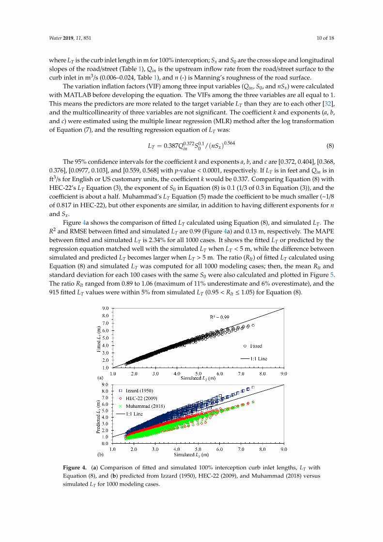
Figure 4a shows the comparison of fitted LT calculated using Equation (8), and simulated LT. TheR2 and RMSE between fitted and simulated LT are 0.99 (Figure 4a) and 0.13 m, respectively. The MAPEbetween fitted and simulated LT is 2.34% for all 1000 cases. It shows the fitted LT or predicted by theregression equation matched well with the simulated LT when LT < 5 m, while the difference betweensimulated and predicted LT becomes larger when LT > 5 m. The ratio (Rlt) of fitted LT calculated usingEquation (8) and simulated LT was computed for all 1000 modeling cases; then, the mean Rlt andstandard deviation for each 100 cases with the same S0 were also calculated and plotted in Figure 5.The ratio Rlt ranged from 0.89 to 1.06 (maximum of 11% underestimate and 6% overestimate), and the915 fitted LT values were within 5% from simulated LT (0.95 < Rlt ≤ 1.05) for Equation (8).

Water 2019, 11, x 10 of 18

surface to the curb inlet in m3/s (0.006–0.024, Table 1), and n (-) is Manning’s roughness of the road surface.

The variation inflation factors (VIF) among three input variables (Qin, S0, and nSx) were calculated with MATLAB before developing the equation. The VIFs among the three variables are all equal to 1. This means the predictors are more related to the target variable LT than they are to each other [32], and the multicollinearity of three variables are not significant. The coefficient k and exponents (a, b, and c) were estimated using the multiple linear regression (MLR) method after the log transformation of Equation (7), and the resulting regression equation of LT was: 𝐿 = 0.387𝑄 . 𝑆 . /(𝑛𝑆 ) . (8)

The 95% confidence intervals for the coefficient k and exponents a, b, and c are [0.372, 0.404], [0.368, 0.376], [0.0977, 0.103], and [0.559, 0.568] with p-value < 0.0001, respectively. If LT is in feet and Qin is in ft3/s for English or US customary units, the coefficient k would be 0.337. Comparing Equation (8) with HEC-22′s LT Equation (3), the exponent of S0 in Equation (8) is 0.1 (1/3 of 0.3 in Equation (3)), and the coefficient is about a half. Muhammad’s LT Equation (5) made the coefficient to be much smaller (~1/8 of 0.817 in HEC-22), but other exponents are similar, in addition to having different exponents for n and Sx.

Figure 4a shows the comparison of fitted LT calculated using Equation (8), and simulated LT. The R2 and RMSE between fitted and simulated LT are 0.99 (Figure 4a) and 0.13 m, respectively. The MAPE between fitted and simulated LT is 2.34% for all 1000 cases. It shows the fitted LT or predicted by the regression equation matched well with the simulated LT when LT < 5 m, while the difference between simulated and predicted LT becomes larger when LT > 5 m. The ratio (Rlt) of fitted LT calculated using Equation (8) and simulated LT was computed for all 1000 modeling cases; then, the mean Rlt and standard deviation for each 100 cases with the same S0 were also calculated and plotted in Figure 5. The ratio Rlt ranged from 0.89 to 1.06 (maximum of 11% underestimate and 6% overestimate), and the 915 fitted LT values were within 5% from simulated LT (0.95 Rlt 1.05) for Equation (8).

Figure 4. (a) Comparison of fitted and simulated 100% interception curb inlet lengths, LT with Equation (8), and (b) predicted from Izzard (1950), HEC-22 (2009), and Muhammad (2018) versus simulated LT for 1000 modeling cases.

Figure 4. (a) Comparison of fitted and simulated 100% interception curb inlet lengths, LT withEquation (8), and (b) predicted from Izzard (1950), HEC-22 (2009), and Muhammad (2018) versussimulated LT for 1000 modeling cases.

Water 2019, 11, 851 11 of 18

Water 2019, 11, x 11 of 18

Figure 5. The mean ratio Rlt of fitted/predicted and simulated LT as a function of longitudinal slope S0 for 1000 modeling cases with standard deviations.

Figure 4b shows a comparison of predicted LT results with Izzard (1950), HEC-22 (2009), and Muhammad (2018) methods to the simulated results, and the corresponding predicted LT in m has ranges of [1.12, 8.60], [0.78, 6.36], and [0.63, 6.27], respectively. The predicted LT for all three methods had strongly linear correlations with simulated LT with R2 of 0.91–0.97. The MAPEs between predicted from HEC-22 (2009), Izzard (1950), and Muhammad (2018) and simulated LT for all 1000 cases were 22.4%, 14.0%, and 32.3%, respectively; the corresponding RMSEs were 0.13 m, 0.22 m, and 1.01 m. The HEC-22 and Muhammad methods underestimate LT with Rlt ranging from 0.48 to 0.92 (0.78 ± 0.10 for average and standard deviation) and from 0.39 to 0.84 (0.68 ± 0.09), respectively. The Rlt range for Izzard method was [0.70, 1.28] with an average and standard deviation of 1.08 and 0.13. For the Izzard method, 771 cases overestimated the simulated LT.

Figure 5 shows the average plus/minus the standard deviation of Rlt for Equation (8), Izzard (1950), HEC-22 (2009), and Muhammad (2018) with respect to different S0 values. All mean Rlt ratios were within the range [0.95, 1.05] with small standard deviations (0.02–0.03) for fitted Equation (8), which indicate that the Equation (8) matches very well with simulated LT for all S0 conditions. For HEC-22 and Muhammad methods, Rlt < 0.95 for all S0 situations and the Muhammad method has a larger standard deviation (0.05–0.07), which means the HEC-22 and Muhammad methods underestimate LT in a greater extent under smaller S0 situations. For the Izzard method, most of Rlt 1 (overestimates LT) when S0 0.3%, and it underestimates LT when S0 0.3%. For three previous methods, the mean Rlt strongly correlates with S0 as a power function with R2 > 0.97 (Figure 5): Rlt increases with the increase of S0.

3.4. 100% Intercepted Gutter Flow for Drainage and Road Bioretention Design

The simulated LT ranged from 1.61 to 7.56 m for the 1000 modeling cases (Figure 4a). In urban drainage design, the inlet opening lengths for various types of curb inlets standardized by municipalities and transportation agencies have only a few preset/pre-cast/manufactured lengths; for example, Texas Type C and Type D curb inlets [7] and TxDOT precast curb inlet outside roadway (PCO) on-grade curb inlets [31] have three opening lengths of 1.52 m (5 ft), 3.05 m (10 ft), and 4.57 m (15 ft). When the calculated curb inlet length for 100% interception is large under design gutter flow, none of the very large opening curb inlets are actually used, but continuously depressed gutter or locally depressed inlets with necessary transient lengths are typically designed and built. Therefore, Equation (8) from the current study, Equation (1) from Izzard (1950), Equation (3) from HEC-22 (2009), and Equation (5) from Muhammad (2018) were rearranged to determine the gutter flow for 100% interception (Qg100) when the curb inlet length is given.

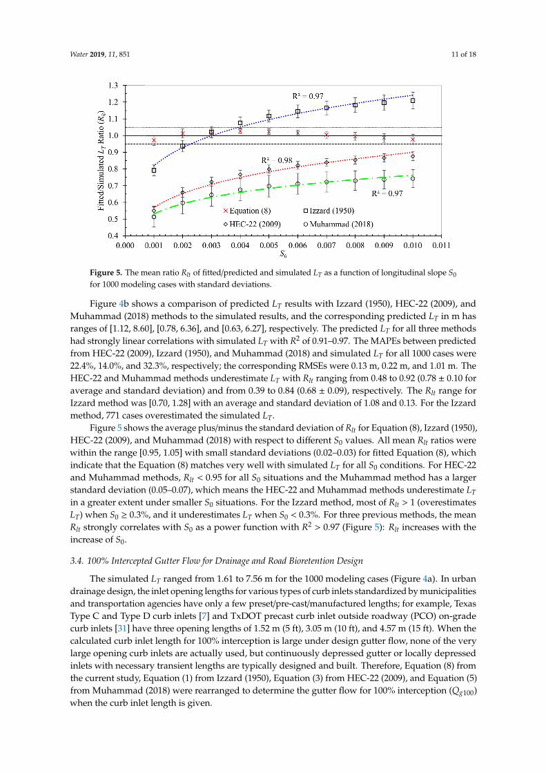
Figure 5. The mean ratio Rlt of fitted/predicted and simulated LT as a function of longitudinal slope S0

for 1000 modeling cases with standard deviations.

Figure 4b shows a comparison of predicted LT results with Izzard (1950), HEC-22 (2009), andMuhammad (2018) methods to the simulated results, and the corresponding predicted LT in m hasranges of [1.12, 8.60], [0.78, 6.36], and [0.63, 6.27], respectively. The predicted LT for all three methodshad strongly linear correlations with simulated LT with R2 of 0.91–0.97. The MAPEs between predictedfrom HEC-22 (2009), Izzard (1950), and Muhammad (2018) and simulated LT for all 1000 cases were22.4%, 14.0%, and 32.3%, respectively; the corresponding RMSEs were 0.13 m, 0.22 m, and 1.01 m. TheHEC-22 and Muhammad methods underestimate LT with Rlt ranging from 0.48 to 0.92 (0.78 ± 0.10 foraverage and standard deviation) and from 0.39 to 0.84 (0.68 ± 0.09), respectively. The Rlt range forIzzard method was [0.70, 1.28] with an average and standard deviation of 1.08 and 0.13. For the Izzardmethod, 771 cases overestimated the simulated LT.

Figure 5 shows the average plus/minus the standard deviation of Rlt for Equation (8), Izzard (1950),HEC-22 (2009), and Muhammad (2018) with respect to different S0 values. All mean Rlt ratios werewithin the range [0.95, 1.05] with small standard deviations (0.02–0.03) for fitted Equation (8), whichindicate that the Equation (8) matches very well with simulated LT for all S0 conditions. For HEC-22and Muhammad methods, Rlt < 0.95 for all S0 situations and the Muhammad method has a largerstandard deviation (0.05–0.07), which means the HEC-22 and Muhammad methods underestimate LTin a greater extent under smaller S0 situations. For the Izzard method, most of Rlt > 1 (overestimatesLT) when S0 ≥ 0.3%, and it underestimates LT when S0 < 0.3%. For three previous methods, the meanRlt strongly correlates with S0 as a power function with R2 > 0.97 (Figure 5): Rlt increases with theincrease of S0.

3.4. 100% Intercepted Gutter Flow for Drainage and Road Bioretention Design

The simulated LT ranged from 1.61 to 7.56 m for the 1000 modeling cases (Figure 4a). In urbandrainage design, the inlet opening lengths for various types of curb inlets standardized by municipalitiesand transportation agencies have only a few preset/pre-cast/manufactured lengths; for example, TexasType C and Type D curb inlets [7] and TxDOT precast curb inlet outside roadway (PCO) on-gradecurb inlets [31] have three opening lengths of 1.52 m (5 ft), 3.05 m (10 ft), and 4.57 m (15 ft). When thecalculated curb inlet length for 100% interception is large under design gutter flow, none of the verylarge opening curb inlets are actually used, but continuously depressed gutter or locally depressedinlets with necessary transient lengths are typically designed and built. Therefore, Equation (8) fromthe current study, Equation (1) from Izzard (1950), Equation (3) from HEC-22 (2009), and Equation (5)from Muhammad (2018) were rearranged to determine the gutter flow for 100% interception (Qg100)when the curb inlet length is given.

Water 2019, 11, 851 12 of 18

Qg100 = 12.832(nSx)1.516L2.688

ci /S0.2690 (9)

Qg100−Izzard = 0.410(nSx)9/7L16/7

ci /S9/140 (10)

Qg100−HEC−22 = 1.618(nSx)1.429L2.381

ci /S0.7140 (11)

Qg100−Muhammad = 131.360n2.021S1.596x L2.128

ci /S0.5530 (12)

All the above equations are for the International System of Units (SI) where Lci is in m and Qg100 ism3/s. Determining Qg100 helps us to reevaluate these LT equations. For urban drainage design, designdischarge for the gutter was calculated first based on the catchment area, runoff coefficients of landuse, and design rainfall intensity; then, the distance between two curb inlets and the curb inlet openingwere calculated and selected/specified for the design.

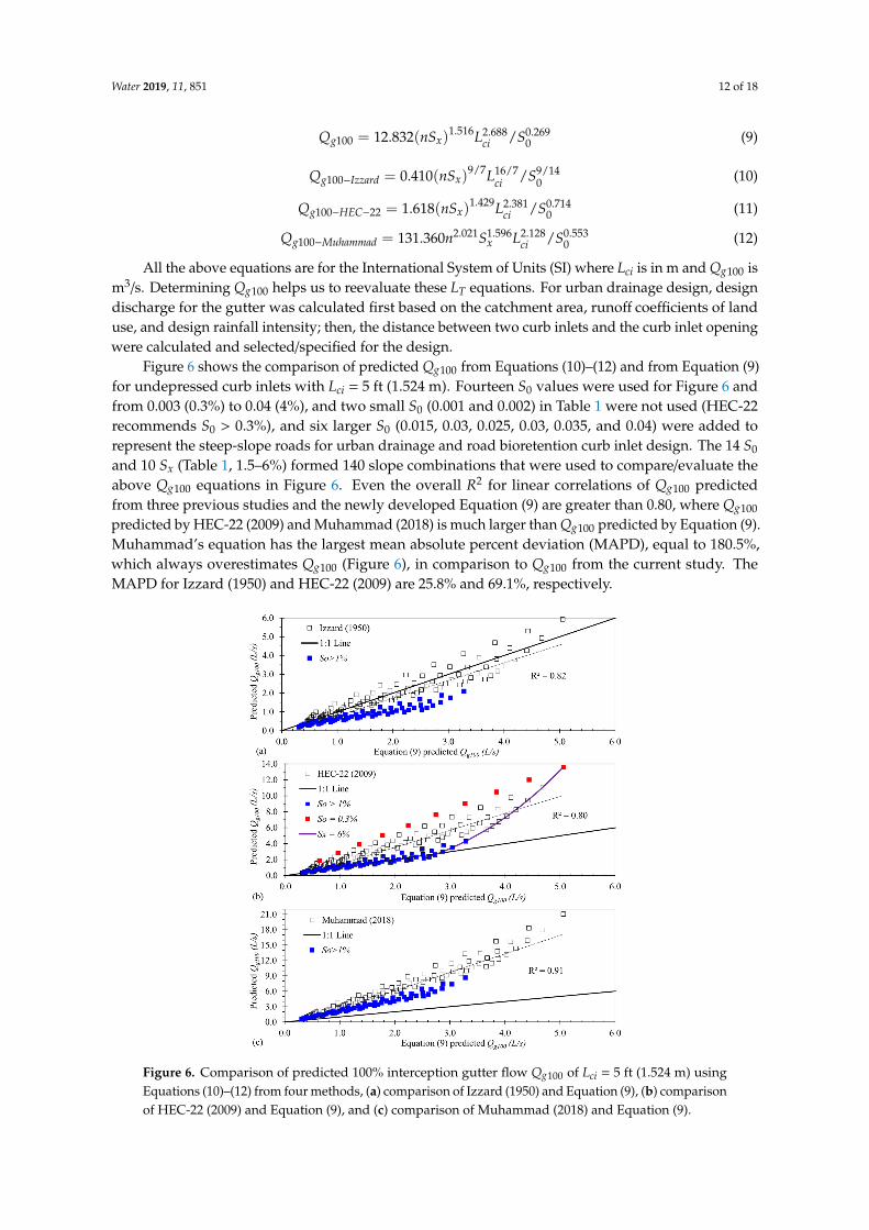
Figure 6 shows the comparison of predicted Qg100 from Equations (10)–(12) and from Equation (9)for undepressed curb inlets with Lci = 5 ft (1.524 m). Fourteen S0 values were used for Figure 6 andfrom 0.003 (0.3%) to 0.04 (4%), and two small S0 (0.001 and 0.002) in Table 1 were not used (HEC-22recommends S0 > 0.3%), and six larger S0 (0.015, 0.03, 0.025, 0.03, 0.035, and 0.04) were added torepresent the steep-slope roads for urban drainage and road bioretention curb inlet design. The 14 S0

and 10 Sx (Table 1, 1.5–6%) formed 140 slope combinations that were used to compare/evaluate theabove Qg100 equations in Figure 6. Even the overall R2 for linear correlations of Qg100 predictedfrom three previous studies and the newly developed Equation (9) are greater than 0.80, where Qg100

predicted by HEC-22 (2009) and Muhammad (2018) is much larger than Qg100 predicted by Equation (9).Muhammad’s equation has the largest mean absolute percent deviation (MAPD), equal to 180.5%,which always overestimates Qg100 (Figure 6), in comparison to Qg100 from the current study. TheMAPD for Izzard (1950) and HEC-22 (2009) are 25.8% and 69.1%, respectively.

Water 2019, 11, x 12 of 18

𝑄 = 12.832(𝑛𝑆 ) . 𝐿 . /𝑆 . (9) 𝑄 = 0.410(𝑛𝑆 ) / 𝐿 / /𝑆 / (10) 𝑄 = 1.618(𝑛𝑆 ) . 𝐿 . /𝑆 . (11) 𝑄 = 131.360𝑛 . 𝑆 . 𝐿 . /𝑆 . (12)

All the above equations are for the International System of Units (SI) where Lci is in m and Qg100 is m3/s. Determining Qg100 helps us to reevaluate these LT equations. For urban drainage design, design discharge for the gutter was calculated first based on the catchment area, runoff coefficients of land use, and design rainfall intensity; then, the distance between two curb inlets and the curb inlet opening were calculated and selected/specified for the design.

Figure 6 shows the comparison of predicted Qg100 from Equations (10)–(12) and from Equation (9) for undepressed curb inlets with Lci = 5 ft (1.524 m). Fourteen S0 values were used for Figure 6 and from 0.003 (0.3%) to 0.04 (4%), and two small S0 (0.001 and 0.002) in Table 1 were not used (HEC-22 recommends S0 > 0.3%), and six larger S0 (0.015, 0.03, 0.025, 0.03, 0.035, and 0.04) were added to represent the steep-slope roads for urban drainage and road bioretention curb inlet design. The 14 S0 and 10 Sx (Table 1, 1.5–6%) formed 140 slope combinations that were used to compare/evaluate the above Qg100 equations in Figure 6. Even the overall R2 for linear correlations of Qg100 predicted from three previous studies and the newly developed Equation (9) are greater than 0.80, where Qg100 predicted by HEC-22 (2009) and Muhammad (2018) is much larger than Qg100 predicted by Equation (9). Muhammad’s equation has the largest mean absolute percent deviation (MAPD), equal to 180.5%, which always overestimates Qg100 (Figure 6), in comparison to Qg100 from the current study. The MAPD for Izzard (1950) and HEC-22 (2009) are 25.8% and 69.1%, respectively.

Figure 6. Comparison of predicted 100% interception gutter flow Qg100 of Lci = 5 ft (1.524 m) using Equations (10)–(12) from four methods, (a) comparison of Izzard (1950) and Equation (9), (b)

Figure 6. Comparison of predicted 100% interception gutter flow Qg100 of Lci = 5 ft (1.524 m) usingEquations (10)–(12) from four methods, (a) comparison of Izzard (1950) and Equation (9), (b) comparisonof HEC-22 (2009) and Equation (9), and (c) comparison of Muhammad (2018) and Equation (9).

Water 2019, 11, 851 13 of 18

Hodges et al. [31] compared Qg100 predicted using HEC-22 equation and their experimentalmeasurements. When Sx was fixed at 6% and S0 changed from 4% to 0.1%, the Qg100 predicted usingthe HEC-22 equation increased about 6 times, but experimental measurements only increased less than1.6 times. The purple line on Figure 6b shows the comparison of HEC-22 and Equation (9) predictedQg100 results when Sx = 0.06 (6%). When S0 decreased from 4% to 0.3% at Sx = 6%, Qg100 calculatedusing HEC-22 increased 6.4 times but Qg100 from Equation (9) only increased two times, which issimilar to results from the physical model by Hodges et al. [31]. The smaller exponent 0.269 for S0

in Equation (9) for the current study seems to give a better prediction on Qg100 compared to HEC-22Equation (11).

In Figure 6b, 10 red filled squares gave Qg100 predicted from HEC-22 for S0 = 0.3%, and Sx increasedfrom 1.5% to 6%, and Qg100 increased from 1.8 L/s to 13.6 L/s that was, on average, 2.83 times largerthan Qg100 (0.62–5.1 L/s) from Equation (9). At S0 = 0.3%, the ratio of Qg100 predicted from HEC-22 toEquation (9) ranged from 2.69 to 3.03 with a standard deviation from the mean of 0.11, which graphicallyshows as a perfect linear relation of these red filled squares on Figure 6b. This strong linear correlationof Qg100 predicted from three previous studies versus Equation (9) exists for all other S0 when Sx ischanged. The ratio of Qg100 predicted from HEC-22 (2009) versus Equation (9) ranges from 0.85 to 3.03,and has a strong correlation with the longitudinal slope S0: a power function Qg100-HEC-22/Qg100-Equation-9

= 0.213 S0−0.445 (R2 = 0.99). Actually, the power function can be approximately derived by dividing

Equation (11) to Equation (9). The power function clearly indicates that over-prediction occurs insmaller S0 because of the negative exponent −0.445; for example, S0 = 0.3%, as shown by the redfilled squares. The blue filled squares on Figure 6 show results for 60 cases with S0 > 1% and Sx from1.5% to 4%. From the power function, when S0 is larger, the ratio of Qg100 is smaller, as is also clearlyshown in Figure 6 by the blue filled squares for all three methods. Figure 6b shows that the predictedQg100 from HEC-22 matched very well with the ones predicted from Equation (9) when S0 > 1%. Thismeans both HEC-22 and the newly developed Equation (9) do a very good job to predict Qg100 (orLT using Equation 8) when S0 > 1%. HEC-22’s Equation (3) for LT and rearranged Equation (11) forQg100 have exponents for slopes S0 and Sx that were adjusted from Izzard’s Equation (1) using limitedavailable experiments, but HEC-22 did not document clearly what specific experimental data wereused, which could be for experiments S0 > 1%. The over-prediction of HEC-22 on Qg100 actually onlyoccurs at lower longitudinal slopes; this could be because the HEC-22 equation was not adjusted withexperimental data of small S0. The ratio of Qg100 predicted from HEC-22 (2009) versus Equation (9)also seems to correlate with the ratio Sx/S0 and becomes larger (over-prediction) when the ratio Sx/S0

increases. The power function of the Qg100 ratio versus the ratio Sx/S0 has a determination coefficientof 0.69, which is much weaker than the correlation with S0 only (R2 = 0.99).

Hodges et al. [31] also show that, when the curb length Lci = 10 ft, Sx was fixed at 6%, and S0

changed from 4% to 0.1%, Qg100 calculated using HEC-22 equation over-predicts by an average factorof 1.51 when compared to measured Qg100 from their physical model. The ratio of Qg100 predicted fromHEC-22 (2009) versus measurements actually ranges from 0.81 to 3.0, and the ratio of Qg100 predictedfrom HEC-22 versus Equation (9) also ranges from 0.85 to 2.37 (Figure 6), and these two results arevery similar. The comparison of predicted 100% intercepted gutter flow with Equations (10)–(12) toEquation (9) for curb length Lci = 10 ft (3.048 m) and Lci = 15 ft (4.572 m) also gives similar resultsdiscussed above for Lci = 5 ft (1.524 m) cases, and are therefore not repeated here.

3.5. Simulated Curb Inlet Efficiency and Evaluation Equation

Table 1 shows Eci determined for 10 example cases (OmXmLm, m = 1, 2, . . . , 10), which rangefrom 15.3–75.7%. Eci was calculated as the curb inlet outflow divided by the upstream inflow (Figure 1)when the flow through the curb inlet reaches the equilibrium—in other words, the Eci change is lessthan 0.0005. For the second set of 1000 modeling cases (O1X1L1 to O10X10L1) of 10 different Lci values(Table 1), the mean and standard deviations of simulated Eci at the same Lci were calculated. The meanEci increased from 12.8% to 84.2%, and the corresponding standard deviation increased from 5.2% to

Water 2019, 11, 851 14 of 18

11.8% when Lci increased from 0.15 m to 1.50 m. This means inlets in the Philadelphia area (the surveyconducted by Stoolmiller et al. [5]) could intercept different amounts of stormwater runoff to roadbioretention facilities, and some of them were under-designed and had flooding risks on the road.

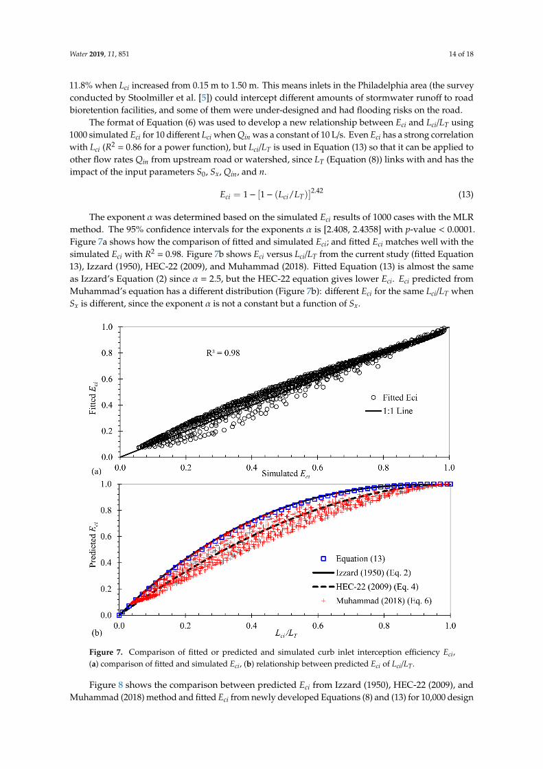
The format of Equation (6) was used to develop a new relationship between Eci and Lci/LT using1000 simulated Eci for 10 different Lci when Qin was a constant of 10 L/s. Even Eci has a strong correlationwith Lci (R2 = 0.86 for a power function), but Lci/LT is used in Equation (13) so that it can be applied toother flow rates Qin from upstream road or watershed, since LT (Equation (8)) links with and has theimpact of the input parameters S0, Sx, Qin, and n.

Eci = 1− [1− (Lci/LT)]2.42 (13)

The exponent α was determined based on the simulated Eci results of 1000 cases with the MLRmethod. The 95% confidence intervals for the exponents α is [2.408, 2.4358] with p-value < 0.0001.Figure 7a shows how the comparison of fitted and simulated Eci; and fitted Eci matches well with thesimulated Eci with R2 = 0.98. Figure 7b shows Eci versus Lci/LT from the current study (fitted Equation13), Izzard (1950), HEC-22 (2009), and Muhammad (2018). Fitted Equation (13) is almost the sameas Izzard’s Equation (2) since α = 2.5, but the HEC-22 equation gives lower Eci. Eci predicted fromMuhammad’s equation has a different distribution (Figure 7b): different Eci for the same Lci/LT whenSx is different, since the exponent α is not a constant but a function of Sx.

Water 2019, 11, x 14 of 18

Eci increased from 12.8% to 84.2%, and the corresponding standard deviation increased from 5.2% to 11.8% when Lci increased from 0.15 m to 1.50 m. This means inlets in the Philadelphia area (the survey conducted by Stoolmiller et al. [5]) could intercept different amounts of stormwater runoff to road bioretention facilities, and some of them were under-designed and had flooding risks on the road.

The format of Equation (6) was used to develop a new relationship between Eci and Lci/ LT using 1000 simulated Eci for 10 different Lci when Qin was a constant of 10 L/s. Even Eci has a strong correlation with Lci (R2 = 0.86 for a power function), but Lci/LT is used in Equation (13) so that it can be applied to other flow rates Qin from upstream road or watershed, since LT (Equation (8)) links with and has the impact of the input parameters S0, Sx, Qin, and n. 𝐸 = 1 − [1 − (𝐿 /𝐿 )] . (13)

The exponent 𝛼 was determined based on the simulated Eci results of 1000 cases with the MLR method. The 95% confidence intervals for the exponents 𝛼 is [2.408, 2.4358] with p-value < 0.0001. Figure 7a shows how the comparison of fitted and simulated Eci; and fitted Eci matches well with the simulated Eci with R2 = 0.98. Figure 7b shows Eci versus Lci/LT from the current study (fitted Equation 13), Izzard (1950), HEC-22 (2009), and Muhammad (2018). Fitted Equation (13) is almost the same as Izzard’s equation (2) since 𝛼 = 2.5, but the HEC-22 equation gives lower Eci. Eci predicted from Muhammad’s equation has a different distribution (Figure 7b): different Eci for the same Lci/LT when Sx is different, since the exponent 𝛼 is not a constant but a function of Sx.

Figure 7. Comparison of fitted or predicted and simulated curb inlet interception efficiency Eci, (a) comparison of fitted and simulated Eci, (b) relationship between predicted Eci of Lci/ LT.

Figure 8 shows the comparison between predicted Eci from Izzard (1950), HEC-22 (2009), and Muhammad (2018) method and fitted Eci from newly developed Equations (8) and (13) for 10,000 design cases that are all combinations for 10 S0, 10 Sx, 10 Qin, and 10 Lci listed in Table 1. The

Figure 7. Comparison of fitted or predicted and simulated curb inlet interception efficiency Eci,(a) comparison of fitted and simulated Eci, (b) relationship between predicted Eci of Lci/LT.

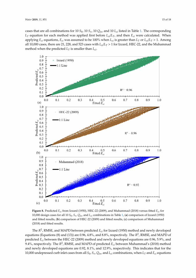
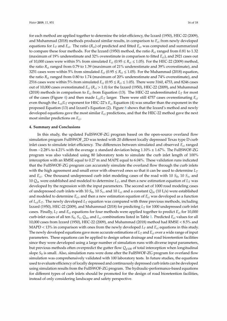
Figure 8 shows the comparison between predicted Eci from Izzard (1950), HEC-22 (2009), andMuhammad (2018) method and fitted Eci from newly developed Equations (8) and (13) for 10,000 design

Water 2019, 11, 851 15 of 18

cases that are all combinations for 10 S0, 10 Sx, 10 Qin, and 10 Lci listed in Table 1. The correspondingLT equation for each method was applied first before Lci/LT, and then Eci were calculated. Whenapplying Eci equations, Eci was assumed to be 100% when Lci is greater than LT or Lci/LT > 1. Amongall 10,000 cases, there are 21, 228, and 523 cases with Lci/LT > 1 for Izzard, HEC-22, and the Muhammadmethod when the predicted LT is smaller than Lci.

Water 2019, 11, x 15 of 18

corresponding LT equation for each method was applied first before Lci/LT, and then Eci were calculated. When applying Eci equations, Eci was assumed to be 100% when Lci is greater than LT or Lci/LT > 1. Among all 10,000 cases, there are 21, 228, and 523 cases with Lci/LT > 1 for Izzard, HEC-22, and the Muhammad method when the predicted LT is smaller than Lci.

Figure 8. Predicted Eci from Izzard (1950), HEC-22 (2009), and Muhammad (2018) versus fitted Eci for 10,000 design cases for all 10 S0, Sx, Qin, and Lci combinations in Table 1, (a) comparison of Izzard (1950) and fitted results, (b) comparison of HEC-22 (2009) and fitted results, (c) comparison of Muhammad (2018) and fitted results.

The R2, RMSE, and MAPD between predicted Eci for Izzard (1950) method and newly developed equations (Equations (8) and (13)) are 0.96, 4.8%, and 8.8%, respectively. The R2, RMSE, and MAPD of predicted Eci between the HEC-22 (2009) method and newly developed equations are 0.96, 5.9%, and 9.4%, respectively. The R2, RMSE, and MAPD of predicted Eci between Muhammad’s (2018) method and newly developed equations are 0.92, 8.1%, and 12.9%, respectively. This indicates that for the 10,000 undepressed curb inlet cases from all S0, Sx, Qin, and Lci combinations, when LT and Eci equations for each method are applied together to determine the inlet efficiency, the Izzard (1950), HEC-22 (2009), and Muhammad (2018) methods produced similar results, in comparison to Eci from

Figure 8. Predicted Eci from Izzard (1950), HEC-22 (2009), and Muhammad (2018) versus fitted Eci for10,000 design cases for all 10 S0, Sx, Qin, and Lci combinations in Table 1, (a) comparison of Izzard (1950)and fitted results, (b) comparison of HEC-22 (2009) and fitted results, (c) comparison of Muhammad(2018) and fitted results.

The R2, RMSE, and MAPD between predicted Eci for Izzard (1950) method and newly developedequations (Equations (8) and (13)) are 0.96, 4.8%, and 8.8%, respectively. The R2, RMSE, and MAPD ofpredicted Eci between the HEC-22 (2009) method and newly developed equations are 0.96, 5.9%, and9.4%, respectively. The R2, RMSE, and MAPD of predicted Eci between Muhammad’s (2018) methodand newly developed equations are 0.92, 8.1%, and 12.9%, respectively. This indicates that for the10,000 undepressed curb inlet cases from all S0, Sx, Qin, and Lci combinations, when LT and Eci equations

Water 2019, 11, 851 16 of 18

for each method are applied together to determine the inlet efficiency, the Izzard (1950), HEC-22 (2009),and Muhammad (2018) methods produced similar results, in comparison to Eci from newly developedequations for LT and Eci. The ratio (Rci) of predicted and fitted Eci was computed and summarizedto compare these four methods. For the Izzard (1950) method, the ratio Rci ranged from 0.81 to 1.32(maximum of 19% underestimate and 32% overestimate in comparison to fitted Eci), and 2921 cases outof 10,000 cases were within 5% from simulated Eci (0.95 ≤ Rci ≤ 1.05). For the HEC-22 (2009) method,the ratio Rci ranged from 0.79 to 1.39 (maximum of 21% underestimate and 39% overestimate), and3251 cases were within 5% from simulated Eci (0.95 ≤ Rci ≤ 1.05). For the Muhammad (2018) equation,the ratio Rci ranged from 0.80 to 1.74 (maximum of 20% underestimate and 74% overestimate), and2516 cases were within 5% from simulated Eci (0.95 ≤ Rci ≤ 1.05). There were 3160, 4753, and 8246 casesout of 10,000 cases overestimated Eci (Rci > 1.0) for the Izzard (1950), HEC-22 (2009), and Muhammad(2018) methods in comparison to Eci from Equation (13). The HEC-22 underestimated LT for mostof the cases (Figure 4) and then made Lci/LT larger. There were still 4757 cases overestimating Ecieven though the Lci/LT exponent for HEC-22’s Eci Equation (4) was smaller than the exponent in theproposed Equation (13) and Izzard’s Equation (2). Figure 8 shows that the Izzard’s method and newlydeveloped equations gave the most similar Eci predictions, and that the HEC-22 method gave the nextmost similar predictions on Eci.

4. Summary and Conclusions

In this study, the updated FullSWOF-ZG program based on the open-source overland flowsimulation program FullSWOF_2D was tested with 20 different locally depressed Texas type D curbinlet cases to simulate inlet efficiency. The differences between simulated and observed Eci rangedfrom −2.28% to 4.21% with the average ± standard deviation being 1.10% ± 1.67%. The FullSWOF-ZGprogram was also validated using 80 laboratory tests to simulate the curb inlet length of 100%interception with an RMSE equal to 0.27 m and MAPE equal to 6.04%. These validation runs indicatedthat the FullSWOF-ZG program can accurately simulate the overland flow through the curb inletswith the high agreement and small error with observed ones so that it can be used to determine LTand Eci. One thousand undepressed curb inlet modeling cases of the road with 10 S0, 10 Sx, and10 Qin were established and modeled to determine LT, and then a new estimation equation of LT wasdeveloped by the regression with the input parameters. The second set of 1000 road modeling casesof undepressed curb inlets with 10 S0, 10 Sx, and 10 Lci and a constant Qin (10 L/s) were establishedand modeled to determine Eci, and then a new estimation equation of Eci was developed as a functionof Lci/LT. The newly developed LT equation was compared with three previous methods, includingIzzard (1950), HEC-22 (2009), and Muhammad (2018) for predicting LT for 1000 undepressed curb inletcases. Finally, LT and Eci equations for four methods were applied together to predict Eci for 10,000curb-inlet cases of all ten S0, Sx, Qin, and Lci combinations listed in Table 1. Predicted Eci values for all10,000 cases from Izzard (1950), HEC-22 (2009), and Muhammad (2018) method had RMSE < 8.5% andMAPD < 13% in comparison with ones from the newly developed LT and Eci equations in this study.The newly developed equations gave more accurate estimations of LT and Eci over a wide range of inputparameters. These equations can be applied to design urban drainage and road bioretention facilitiessince they were developed using a large number of simulation runs with diverse input parameters,but previous methods often overpredict the gutter flow Qg100 of total interception when longitudinalslope S0 is small. Also, simulation runs were done after the FullSWOF-ZG program for overland flowsimulation was comprehensively validated with 100 laboratory tests. In future studies, the equationsused to evaluate efficiency of locally depressed and continuously depressed curb inlets can be developedusing simulation results from the FullSWOF-ZG program. The hydraulic-performance-based equationsfor different types of curb inlets should be promoted for the design of road bioretention facilities,instead of only considering landscape and safety perspective.

Water 2019, 11, 851 17 of 18

Author Contributions: X.L. updated the FullSWOF_2D program, conducted the simulations and analysis of theresults, prepared the manuscript draft. X.F. supervised the model development, simulation runs, data analysis;and revised the manuscript. G.C., Y.G., J.W. and J.L. provided inputs on the writing, data analysis, and revised themanuscript. All authors made contributions to the study and writing the manuscript.

Funding: The research was partially supported by the National Natural Science Foundation of China (No.51478026), Beijing Higher Education High-Level Teachers Team Construction Program (CIT & TCD 201704055),and Beijing University of Civil Engineering and Architecture Research Fund for Pyramid Talents Development.

Acknowledgments: Thanks to Muhammad Ashraf from the University of Texas at Austin organizing and sharingcurb inlet laboratory experimental data for previous studies. The author, X.L., wishes to express his gratitude tothe Chinese Scholarship Council for financial support pursuing his graduate study at Auburn University.

Conflicts of Interest: The authors declare no conflict of interest.

References

1. Starzec, M.; Dziopak, J.; Słys, D.; Pochwat, K.; Kordana, S. Dimensioning of Required Volumes ofInterconnected Detention Tanks Taking into Account the Direction and Speed of Rain Movement. Water2018, 10, 1826. [CrossRef]

2. Li, X.; Li, J.; Fang, X.; Gong, Y.; Wang, W. Case studies of the sponge city program in China. In Proceedingsof the World Environmental and Water Resources Congress, West Palm Beach, FL, USA, 22–26 May 2016;American Society of Civil Engineers: Reston, VA, USA, 2016; pp. 295–308.

3. Li, X.; Fang, X.; Gong, Y.; Li, J.; Wang, J.; Chen, G.; Li, M.-H. Evaluating the road-bioretention strip systemfrom a hydraulic perspective—Case studies. Water 2018, 10, 1778. [CrossRef]

4. Tu, M.-C.; Traver, R. Clogging impacts on distribution pipe delivery of street runoff to an infiltration bed.Water 2018, 10, 1045. [CrossRef]

5. Stoolmiller, S.; Ebrahimian, A.; Wadzuk, B.M.; White, S. Improving the design of curb openings in greenstormwater infrastructure. In Proceedings of the International Low Impact Development Conference,Nashville, TN, USA, 12–15 August 2018; Environmental & Water Resources Institute: Nashville, TN, USA,2018; pp. 168–176.

6. Liang, X. Hydraulic calculation and design optimization of curb opening in Sponge City construction. ChinaWater Wastewater 2018, 34, 42–45. (In Chinese)

7. Hammonds, M.A.; Holley, E. Hydraulic Characteristics of flush Depressed Curb Inlets and Bridge Deck Drains;FHWA-TX 96-1409-1; Texas Department of Transportation: Austin, TX, USA, 1995.

8. Izzard, C.F. Tentative results on capacity of curb opening inlets. In Proceedings of the 29th Annual Conferenceof the Highway Research Board, Washington, DC, USA, 13–16 December 1949; Highway Research Board:Washington, DC, USA, 1950; pp. 11–13.

9. Li, W.H. Hydraulic theory for design of stormwater inlets. In Proceedings of the 33rd Annual Meetingof the Highway Research Board, Washington, DC, USA, 12–15 January 1954; Highway Research Board:Washington, DC, USA, 1954; pp. 83–91.

10. Brown, S.; Stein, S.; Warner, J. Urban Drainage Design Manual: Hydraulic Engineering Circular No. 22 (HEC-22);FHWA-NHI-10-009 HEC-22; National Highway Institute: Arlington, VA, USA, 2009.

11. Jens, S. Design of Urban Highway Drainage; FHWA-NHI-10-009 HEC-22; Federal Highway Administration:Washington, DC, USA, 1979; pp. 198–226.

12. Johnson, F.L.; Chang, F.F. Drainage of Highway Pavements: Hydraulic Engineering Circular No. 12 (HEC-12);FHWA-TS-84-202 HEC No.12; Federal Highway Administration: McLean, VA, USA, 1984; pp. 39–64.

13. Muhammad, M.A. Interception Capacity of Curb Opening Inlets; University of Texas at Austin: Austin, TX,USA, 2018.

14. Guo, J.C.Y.; MacKenzie, K. Hydraulic Efficiency of Grate and Curb-Opening Inlets Under Clogging Effect(CDOT-2012-3); Colorado Department of Transportation, DTD Applied Research and Innovation Branch:Denver, CO, USA, 2012.

15. Uyumaz, A. Urban drainage with curb-opening inlets. In Proceedings of the Ninth International Conferenceon Urban Drainage (9ICUD), Portland, OR, USA, 8–13 September 2002; American Society of Civil Engineers:Portland, OR, USA, 2002; pp. 1–9.

16. Schalla, F.E.; Ashraf, M.; Barrett, M.E.; Hodges, B.R. Limitations of traditional capacity equations for longcurb inlets. Transp. Res. Rec. 2017, 2638, 97–103. [CrossRef]

Water 2019, 11, 851 18 of 18

17. Comport, B.C.; Thornton, C.I. Hydraulic efficiency of grate and curb inlets for urban storm drainage.J. Hydraul. Eng. 2012, 138, 878–884. [CrossRef]

18. Russo, B.; Gómez, M. Discussion of “hydraulic efficiency of grate and curb inlets for urban storm drainage”by Brendan C. Comport and Christopher I. Thornton. J. Hydraul. Eng. 2013, 140, 121–122. [CrossRef]

19. Wasley, R.J. Hydrodynamics of flow into curb-opening inlets. J. Eng. Mech. Div. 1961, 87, 1–18.20. Delestre, O.; Darboux, F.; James, F.; Lucas, C.; Laguerre, C.; Cordier, S. FullSWOF: A free software package

for the simulation of shallow water flows. arXiv 2014, arXiv:1401.4125.21. Fang, X.; Jiang, S.; Alam, S.R. Numerical simulations of efficiency of curb-opening inlets. J. Hydraul. Eng.

2009, 136, 62–66. [CrossRef]22. Barréde Saint-Venant, A.J.C. Théorie du mouvement non permanent des eaux, avec application aux crues

des rivières et à l’introduction des marées dans leurs lits. Comptes Rendus des Séances de l’Académie des Sciences1871, 73, 237–240.

23. Unterweger, K.; Wittmann, R.; Neumann, P.; Weinzierl, T.; Bungartz, H.-J. Integration of FullSWOF_2D andPeanoClaw: Adaptivity and local time-stepping for complex overland flows. In Recent Trends in ComputationalEngineering-CE2014; Springer: Berlin, Germany, 2015; pp. 181–195.

24. Gourbesville, P.; Cunge, J.; Caignaert, G. Advances in Hydroinformatics-SIMHYDRO 2014, 1st ed.; Springer:Singapore, 2014; p. 624.

25. Zhang, W.; Cundy, T.W. Modeling of two-dimensional overland flow. Water Resour. Res. 1989, 25, 2019–2035.[CrossRef]

26. Audusse, E.; Bouchut, F.; Bristeau, M.-O.; Klein, R.; Perthame, B.T. A fast and stable well-balanced schemewith hydrostatic reconstruction for shallow water flows. SIAM J. Sci. Comput. 2004, 25, 2050–2065. [CrossRef]

27. Cordier, S.; Coullon, H.; Delestre, O.; Laguerre, C.; Le, M.H.; Pierre, D.; Sadaka, G. FullSWOF Paral: Comparisonof Two Parallelization Strategies (MPI and SKELGIS) on a Software Designed for Hydrology Applications; ESAIM:Proceedings; EDP Sciences: Julius, France, 2013; pp. 59–79.

28. Leandro, J.; Martins, R. A methodology for linking 2D overland flow models with the sewer network modelSWMM 5.1 based on dynamic link libraries. Water Sci. Technol. 2016, 73, 3017–3026. [CrossRef] [PubMed]

29. Li, X.; Fang, X.; Li, J.; KC, M.; Gong, Y.; Chen, G. Estimating time of concentration for overland flow onpervious surfaces by particle tracking method. Water 2018, 10, 379. [CrossRef]

30. MathWorks. Matlab and Statistics Toolbox Release 2017a; The MathWorks Inc.: Natick, MA, USA, 2017.31. Hodges, B.R.; Barrett, M.E.; Ashraf, M.; Schalla, F.E. Interception Capacity of Conventional Depressed Curb Inlets

and Inlets with Channel Extension; Texas Department of Transportation: Austin, TX, USA, 2018; pp. 54–57.32. Chatterjee, S.; Simonoff, J.S. Handbook of Regression Analysis; John Wiley & Sons: Hoboken, NJ, USA, 2013;

Volume 5.

© 2019 by the authors. Licensee MDPI, Basel, Switzerland. This article is an open accessarticle distributed under the terms and conditions of the Creative Commons Attribution(CC BY) license (http://creativecommons.org/licenses/by/4.0/).