cross-sectional stability of double inlet systems
TRANSCRIPT

Cross-Sectional Stability of DoubleInlet Systems


Cross-Sectional Stability of DoubleInlet Systems
Proefschrift
ter verkrijging van de graad van doctoraan de Technische Universiteit Delft,
op gezag van de Rector Magnificus prof.ir. K.C.A.M. Luyben,voorzitter van het College voor Promoties,
in het openbaar te verdedigen op maandag 30 september 2013 om 12:30 uurDelft, Nederland
door
Ronald Leendert Brouwerciviel ingenieur
geboren te Hellevoetsluis, Nederland

Dit manuscript is goedgekeurd door de promotor:Prof.dr.dr.h.c.ir. M.J.F. Stive
Copromotor:Dr. H.M. Schuttelaars
Samenstelling promotiecommissie:Rector Magnificus voorzitterProf.dr.dr.h.c.ir. M.J.F. Stive Delft University of Technology, promotorDr. H.M. Schuttelaars Delft University of Technology, copromotorProf.dr.ir. J. van de Kreeke University of MiamiProf.dr.ir. Z.B. Wang Delft University of TechnologyProf.dr.ir. W.S.J. Uijttewaal Delft University of TechnologyProf.dr. L.R.M. Maas NIOZ/Utrecht UniversityDr.ir. P.C. Roos University of Twente
This research has been financially supported by Delft University of Technologyand the Delft Cluster Project: Sustainable development of the North Sea andCoast.
Keywords: barrier coast, tidal inlet system, cross-sectional stability, equilibrium,morphodynamics, entrance/exit losses.
ISBN 978-94-6186-178-8
Copyright c© 2013 by Ronald Brouwer
Printed by GVO drukkers & vormgevers B.V., the Netherlands.
All rights reserved. No part of the material protected by this copyright noticemay be reproduced or utilised in any form or by any means, electronic or me-chanical, including photocopying, recording or by any information storage andretrieval system, without written permission of the author.
Cover image: Author’s impression of the Dutch, German and Danish WaddenSea coast

Advice from the ocean:
Be shore of yourselfCome out of your shellTake time to coastAvoid pier pressureSea life’s beautyDon’t get tide downMake waves!
- Ilan Shamir


Summary
Barrier coasts and their associated tidal inlet systems are a common feature inmany parts of the world. They constitute dynamic environments that are in acontinuous stage of adapting to the prevailing tide and wave conditions. Com-monly, these coastal areas are densely populated and (partly) as a result thereoften exists a strong conflict of interests between issues related to coastal safety,economic activities and ecology. To manage these different interests, it is impor-tant to gain more understanding of the long-term morphological evolution oftidal inlet systems and their adaptation to natural changes and human interven-tion. In this thesis the focus is on double inlet systems, where two tidal inletsconnect a back-barrier basin to an ocean or a coastal sea.
To investigate the morphological evolution of double inlet systems and theiradaptation to internal or external change, the equilibrium configuration and sta-bility properties of the cross-sectional areas of the two tidal inlets are studied indetail. To that extent, a widely used empirical relationship for cross-sectionalinlet stability is combined with (i) a lumped-parameter (L-P) model (Chapters 2and 3) and (ii) a two-dimensional, depth-averaged hydrodynamic (2DH) modelfor the water motion (Chapter 4). The Marsdiep-Vlie inlet system in the west-ern Dutch Wadden Sea and the Faro-Armona inlet system in the Portuguese RıaFormosa serve as case studies throughout this thesis.
With the assumptions of a cross-sectionally averaged, uniform inlet flow ve-locity and a uniformly fluctuating basin surface elevation, model results of theL-P model show that stable equilibrium configurations where both inlets areopen exist. It is necessary, however, to account for the important processes ei-ther explicitly, e.g. including a topographic high in the back-barrier basin as ob-served in the Wadden Sea (Chapter 2), or parametrically, e.g. allowing for inletentrance/exit losses for relatively short inlets such as in the Rıa Formosa (Chap-ter 3).
By solving the depth-averaged, linear shallow water equations on the f -planewith linearised bottom friction, the 2DH model explicitly accounts for spatialvariations in surface elevation in the ocean, inlets and basin. Model results showthat these spatial variations, induced by e.g. basin bottom friction, radiation damp-
i

ii Summary
ing, and Coriolis effects, are crucial to simulate and explain the long-term evo-lution of double inlet systems. This approach further allows the identificationof a stabilising and destabilising mechanism associated with the persistence orclosure of one (or both) of the inlets in a double inlet system and hence with itslong-term evolution.

Samenvatting
Barrierekusten en hun bijbehorende zeegat systemen zijn een veelvoorkomendekustvorm over de hele wereld. Het zijn dynamische omgevingen die zich continuaanpassen aan de heersende getij- en golfcondities. Deze kustgebieden zijn overhet algemeen dichtbevolkt en (mede) daardoor ontstaan er vaak sterke conflictentussen problemen die gerelateerd zijn aan kustveiligheid, economische activitei-ten en ecologie. Om deze conflicten te beheersen is het van groot belang om meerkennis te vergaren over de morfologische, lange termijn ontwikkeling van dezesystemen en hun reactie op natuurlijke veranderingen en menselijke ingrepen. Indeze dissertatie ligt de focus op dubbel zeegat systemen, waarbij twee zeegatenhet achterliggende bekken verbinden met een oceaan of kustzee.
Om de morfologische ontwikkeling van dubbel zeegat systemen en hun aan-passing aan interne en externe veranderingen te onderzoeken, worden in dezedissertatie de evenwichtsconfiguraties en stabiliteitskenmerken van de dwars-doorsneden van de twee zeegaten gedetailleerd bestudeerd. Daarvoor wordter een veelgebruikte empirische relatie voor de stabiliteit van de dwarsdoor-snede van een zeegat gecombineerd met (i) een ’lumped-parameter’ (L-P) model(Hoofdstuk 2 en 3) en (ii) een twee-dimensionaal, diepte-gemiddeld hydrodyna-misch (2DH) model voor de waterbeweging (Hoofdstuk 4). Het Marsdiep-Vliesysteem in de westelijke Nederlandse Waddenzee en het Faro-Armona systeemin de Portugese Rıa Formosa worden gebruikt als casus.
Met de aanname van een dwarsdoorsnede-gemiddelde, uniforme stroom-snelheid door het zeegat en een uniform fluctuerend waterniveau in het bek-ken, laten resultaten van het L-P model zien dat stabiele evenwichtsconfiguraties,waarbij beide zeegaten open zijn, kunnen bestaan. Het is daarbij wel van belangom de belangrijke processes expliciet, bv. door het implementeren van een wan-tij in het bekken zoals geobserveerd wordt in de Waddenzee (Hoofdstuk 2), ofimpliciet, bv. door het toestaan van in- en uittreeverliezen voor korte zeegatenzoals in de Rıa Formosa (Hoofdstuk 3), mee te nemen.
Door de diepte-gemiddelde, ondiep water vergelijkingen met lineaire bodem-wrijving op te lossen, neemt het 2DH model ruimtelijke variaties van het waterni-veau in de oceaan, zeegaten en bekken expliciet mee. Modelresultaten laten zien
iii

iv Samenvatting
dat deze ruimtelijke variaties, opgewekt door bv. bodemwrijving in het bekken,radiale demping in de oceaan en Coriolis effecten, cruciaal zijn om de ontwikke-ling van dubbel zeegat systemen te simuleren en te verklaren. Deze modelbena-dering staat bovendien de identificatie van een stabiliserend en destabiliserendmechanism toe, die gerelateerd zijn aan het open blijven of het sluiten van eenvan de (of beide) zeegaten in een dubbel zeegat systeem en dus met zijn morfo-logische ontwikkeling.

Acknowledgements
While writing these acknowledgements, a lot of thoughts fly around in my head.One of the main thoughts that keeps flying by is:”I can’t believe this chapterhas come to an end”. I have been combining a (semi-)professional field hockeycareer and a scientific education for a long period and I’ve enjoyed every minuteof it. During this period I’ve had the privilege to meet a number of amazingpeople and this thesis would not have been possible without their contribution.Therefore, I devote these acknowledgements to them.
First of all, I’d like to thank Marcel Stive for providing me with the oppor-tunity to start a Ph.D. study and giving me the freedom to combine it with asuccessful (semi-)professional field hockey career. Your support, kindness, hu-man interest and availability (even in hectic times) have made a big impact onme.
Embracing the opportunity to understand a problem even better when a re-sult is totally not what you expect, is one of the insights my daily supervisor,Henk Schuttelaars, taught me. Henk, I cannot express my gratitude enough.Your sense of humour, ability to simplify even the most difficult problems, searchfor perfection and patience with my desire for discussion, made me enjoy everysecond of our cooperation during my Ph.D. study.
Next, I would like to thank Co van de Kreeke for passing on his interest in andpassion for (multiple) tidal inlet systems. Together with Henk, you have guidedme since the start of my M.Sc. thesis to where I am today. Thank you very muchfor introducing me to the scientific community and for your sharp and criticalcomments on every document I sent you. I will always remember our sailingtrip out on Biscayne Bay.
In search for a relatively fast, two-dimensional model for the water motionin a double inlet system, Henk introduced me to Pieter Roos. In my opiniona perfect match. Our mutual fascination for fundamental science, spotting thetiniest and sometimes useless style errors, sports and of course LEGO has led toa good friendship and made our collaboration very fruitful. Working togetherwith you and Henk really made me feel part of a team.
A special thanks goes out to Tjerk Zitman and Howard Southgate. Tjerk for
v

vi Acknowledgements
helping me out when I had modelling and Matlab issues, discussing model re-sults and humorous meetings; and Howard for his curiosity, his interest andproofreading my thesis.
Furthermore, I want to thank my colleagues of the Section of Hydraulic Engi-neering, realising that the list is far from complete. My room-mates (in consecu-tive order): Tomo, thank you for your warm character, the Japanese classes, dinerat your place and of course Nam-myoho-renge-kyo (I remembered); Vana, I re-ally liked our discussions about non-scientific topics; and Marriete, thank you fortaking care of me during the last period of finalising my thesis. Martijn, Matthieu,Sierd, Chu, Meagan: somehow the road to my office always passed your office,no matter from which direction I was coming. Thanks for listening, discussions,lunch and making coming to the office enjoyable every single time. My CoastalDynamics II examination buddies Menno and Sierd (and even earlier Jakob andJasper): It was actually really nice to be able to broaden your knowledge in sucha way. Marije: thanks for sharing your thoughts and listening to mine. Wim:the conversations about snowboard and mountain bike trips always made mewander off and forget about finishing my Ph.D. thesis. The support staff: Chan-tal, Agnes, Judith and Inge, thank you for all those years of helping me with allkinds of issues.
Besides colleagues at the university, a lot of people outside the universitycommunity have contributed in one way or the other. I want to thank my fam-ily, family-in-law, friends, my HC Bloemendaal team-mates and staff and otherfriends from the hockey community for their interest, support, layman’s ques-tions and fun times.
At the time of writing these acknowledgements, I know that during my de-fence I will be supported by Marc and Joris as my paranimphs. I’m already look-ing forward to it.
And last, but certainly not least: Birgit, Kalle, Ronja and Lotta. Where wouldI be without you?
Ronald Brouwer
Hamilton, New ZealandAugust 2013

Contents
Summary i
Samenvatting iii
Acknowledgements v
1 Introduction 11.1 Barrier coasts and tidal inlet systems . . . . . . . . . . . . . . . . . . 11.2 Focus of this study . . . . . . . . . . . . . . . . . . . . . . . . . . . . 41.3 Study sites . . . . . . . . . . . . . . . . . . . . . . . . . . . . . . . . . 4
1.3.1 Marsdiep - Vlie inlet system, the Netherlands . . . . . . . . 51.3.2 Faro-Armona inlet system, Portugal . . . . . . . . . . . . . . 6
1.4 Cross-sectional stability of tidal inlets . . . . . . . . . . . . . . . . . 81.5 Research questions . . . . . . . . . . . . . . . . . . . . . . . . . . . . 131.6 Thesis structure and research approach . . . . . . . . . . . . . . . . 141.A Shape of the Escoffier curve . . . . . . . . . . . . . . . . . . . . . . . 16
2 Influence of a topographic high on cross-sectional inlet stability 212.1 Introduction . . . . . . . . . . . . . . . . . . . . . . . . . . . . . . . . 222.2 Equilibrium and stability . . . . . . . . . . . . . . . . . . . . . . . . . 24
2.2.1 General . . . . . . . . . . . . . . . . . . . . . . . . . . . . . . . 242.2.2 Equilibrium velocity . . . . . . . . . . . . . . . . . . . . . . . 252.2.3 Stability and flow diagram . . . . . . . . . . . . . . . . . . . 27
2.3 Hydrodynamic model . . . . . . . . . . . . . . . . . . . . . . . . . . 312.4 Numerical experiments . . . . . . . . . . . . . . . . . . . . . . . . . . 32
2.4.1 Equilibrium configuration under symmetrical forcing . . . . 332.4.2 Amplitude differences only . . . . . . . . . . . . . . . . . . . 352.4.3 Phase differences only . . . . . . . . . . . . . . . . . . . . . . 38
2.5 Discussion . . . . . . . . . . . . . . . . . . . . . . . . . . . . . . . . . 382.6 Conclusions . . . . . . . . . . . . . . . . . . . . . . . . . . . . . . . . 41
vii

viii Contents
2.A Solution method double inlet system with topographic high . . . . 43
3 Entrance/exit losses and cross-sectional inlet stability 493.1 Introduction . . . . . . . . . . . . . . . . . . . . . . . . . . . . . . . . 503.2 Governing equations and method . . . . . . . . . . . . . . . . . . . . 52
3.2.1 Governing Equations . . . . . . . . . . . . . . . . . . . . . . . 523.2.2 Methods . . . . . . . . . . . . . . . . . . . . . . . . . . . . . . 55
3.3 Entrance/exit losses only . . . . . . . . . . . . . . . . . . . . . . . . 583.3.1 Conditions for stable equilibriums . . . . . . . . . . . . . . . 583.3.2 Physical explanation for the interval of stable equilibriums
when Z1 6= Z2 . . . . . . . . . . . . . . . . . . . . . . . . . . . 603.3.3 Model results . . . . . . . . . . . . . . . . . . . . . . . . . . . 613.3.4 Phase differences and stable equilibriums . . . . . . . . . . . 62
3.4 Bottom friction and inertia . . . . . . . . . . . . . . . . . . . . . . . . 633.4.1 Bottom Friction . . . . . . . . . . . . . . . . . . . . . . . . . . 633.4.2 Inertia . . . . . . . . . . . . . . . . . . . . . . . . . . . . . . . 653.4.3 Relative Importance of the Entrance/Exit Loss Term and
the Bottom Friction Term . . . . . . . . . . . . . . . . . . . . 663.5 Effect of forcing on stable equilibriums . . . . . . . . . . . . . . . . . 683.6 The Faro-Armona double inlet system . . . . . . . . . . . . . . . . . 703.7 Discussion . . . . . . . . . . . . . . . . . . . . . . . . . . . . . . . . . 723.8 Conclusions . . . . . . . . . . . . . . . . . . . . . . . . . . . . . . . . 743.A Entrance/Exit Losses Only . . . . . . . . . . . . . . . . . . . . . . . . 76
3.A.1 Basin Tide and Inlet Velocities . . . . . . . . . . . . . . . . . . 763.A.2 Conditions for Equilibrium Cross-Sections for Z1 6= Z2 . . . 773.A.3 The Role of the Entrance/Exit Loss Coefficient m . . . . . . 78
3.B Entrance/Exit Losses and Bottom Friction . . . . . . . . . . . . . . . 803.C Linear Stability Entrance/Exit Losses Only . . . . . . . . . . . . . . 83
4 Double inlet stability by spatially varying water motion 874.1 Introduction . . . . . . . . . . . . . . . . . . . . . . . . . . . . . . . . 884.2 Model and method . . . . . . . . . . . . . . . . . . . . . . . . . . . . 90
4.2.1 Cross-sectional stability . . . . . . . . . . . . . . . . . . . . . 904.2.2 Hydrodynamic model formulation . . . . . . . . . . . . . . . 904.2.3 Flow diagram . . . . . . . . . . . . . . . . . . . . . . . . . . . 94
4.3 Model Results . . . . . . . . . . . . . . . . . . . . . . . . . . . . . . . 944.3.1 Water motion . . . . . . . . . . . . . . . . . . . . . . . . . . . 954.3.2 Influence of radiation damping, basin bottom friction and
Coriolis effects . . . . . . . . . . . . . . . . . . . . . . . . . . 974.3.3 Influence of basin geometry on cross-sectional stability . . . 103
4.4 Discussion . . . . . . . . . . . . . . . . . . . . . . . . . . . . . . . . . 1054.5 Conclusions . . . . . . . . . . . . . . . . . . . . . . . . . . . . . . . . 1064.A Solution method for the 2DH model for double inlet systems . . . . 108

Contents ix
4.A.1 Wave solutions in a channel of uniform depth . . . . . . . . 1084.A.2 Superposition of wave solutions . . . . . . . . . . . . . . . . 1104.A.3 Collocation technique . . . . . . . . . . . . . . . . . . . . . . 1114.A.4 Iterative procedure to calculate friction coefficients . . . . . 112
5 Conclusions and recommendations 1155.1 Answers to the research questions . . . . . . . . . . . . . . . . . . . 1155.2 Overall conclusions . . . . . . . . . . . . . . . . . . . . . . . . . . . . 1175.3 Recommendations . . . . . . . . . . . . . . . . . . . . . . . . . . . . 118
References 120
List of symbols 131
About the author 135


1Introduction
Double inlet systems, often found along barrier coasts, are coastal systems inwhich two tidal inlets connect a single back-barrier basin to an ocean or a coastalsea. In this thesis the cross-sectional equilibrium configurations of the tidal inletsand their stability properties are investigated, in order to obtain more insight intothe long-term evolution of double inlet systems.
In Section 1.1 a description of barrier coasts and tidal inlet systems is given.With this general background information in mind, the focus of this thesis ismotivated in Section 1.2. Subsequently, in Section 1.3 the Faro-Armona andMarsdiep-Vlie inlet systems are introduced. These systems are used through-out this thesis as typical examples of a double inlet system where the two inletsare directly connected by a channel in the basin and one in which this connec-tion is hindered, but not entirely obstructed, by the presence of a topographichigh1 (also known as tidal watershed or tidal divide). A detailed description ofthe present-day knowledge of cross-sectional stability of tidal inlets is given inSection 1.4. Based on this information, in Section 1.5 the research questions areformulated. Finally, in Section 1.6 the methodology and approach that are usedin this thesis are addressed.
1.1 Barrier coasts and tidal inlet systems
Nowadays, approximately ten percent of the world’s continental coastline con-sists of barrier coasts (Glaeser, 1978). These coasts are a concatenation of tidal
1a topographic high is formed where the tidal waves travelling through two adjacent inletsmeet and sedimentation due to low velocities results in tidal flat formation. They act as semi-permeable barriers that allow a certain degree of water exchange.
1

2 Chapter 1. Introduction
0 0.5 1 1.5 2 2.50
1
2
3
4
5
FA
MV
a) Hayes’ coastal classification
mean wave height [m]
me
an
tid
al ra
ng
e [m
]
b) Sketch tidal inlet system
Figure 1.1: (a) Relationship between tidal range, wave height and coastal morphology modifiedfrom Hayes (1975, 1979). The black dotted curve represents the approximate limit of barrierislands formation. The dots desginated FA and MV indicate the position of the Faro-Armonaand Marsdiep-Vlie double inlet systems in this coastal classification (see text Section 1.3) and(b) Sketch of a single tidal inlet system, showing the different geomorphologic elements and thedominant physical processes and phenomena. From: de Swart & Zimmerman (2009).
inlet systems, in which a tidal basin or back-barrier area is connected to an oceanor a coastal sea by one or more tidal inlets. Many of the barrier coasts foundaround the world formed during the Holocene2 when continental shelves wereflooded owing to sea level rise (e.g. Beets & van der Spek, 2000).
Apart from the geological setting, barrier coasts and the associated tidal inletsystems are primarily shaped under the influence of tides and waves. Astro-nomical tides induce both variations in water elevation and currents, with tidalcurrents in the inlet in the order of 1 m s−1. Wind-induced surface waves break inshallow areas inducing wave-driven currents of approximately 1 m s−1. Finally,riverine outflow (when present) will also affect the current in the inlet.
Since waves and tides are important, barrier coasts have been classified us-ing wave height and tidal range. Hayes (1975, 1979) extended the classificationintroduced by Davies (1964) from three to five categories ranging from tide-dominated to wave-dominated coasts; see Fig. 1.1a. Later, Davis Jr. & Hayes(1984) emphasised that it is the relative effect of tides and waves that determinesthe coastal morphotype, not the absolute values of the two. Other factors that
2the Holocene is the present interglacial period, starting at approximately 10,000 years B.P.

1.1. Barrier coasts and tidal inlet systems 3
need to be taken into consideration when dealing with tidal inlets are: coastalphysiography, tidal prism, availability of sediment and influence of riverine in-put. Consequently, barrier coasts that belong to a certain category based on waveheight and tidal range alone can display coastal features of another category be-cause of the influence of the aforementioned factors. In this thesis, mixed-energycoasts are considered where the coastal morphotype displays tide-dominatedcharacteristics, such as short, drumstick-shaped barriers with well-developedebb deltas (see grey area in Fig. 1.1a).
Now focussing on tidal inlet systems in sandy environments, several morpho-logical elements can be discerned; see Fig. 1.1b. On the seaward side of the inleta shallow ebb-tidal delta is often found that usually folds around a deep channel.On the landward side of the inlet sometimes a flood delta is observed. Inside thebasin, the main channels become shallower when moving away from the inlet.Typically, they undergo a sequence of bifurcations resulting in a complex patternof channels and tidal flats. Salt marshes are commonly found near the coastlinesof the mainland and the barrier islands (de Swart & Zimmerman, 2009).
Conceptually, waves and tides can also explain the morphodynamics of tidalinlet systems (see Fig. 1.1b). Obliquely incident waves generate alongshore cur-rents thus triggering alongshore transport of sediment, the so-called littoral drift.When this sediment reaches the downdrift side of a barrier island adjacent to aninlet, part of it is transported past the inlet to the updrift part of the next barrierisland by bar bypassing. This process moves sediment along the seaward portionof the ebb-tidal delta towards the downdrift shore. Another part is transportedpast the inlet by tidal flow bypassing, in which the sediment enters the inlet onflood tide, deposits there and is exported seaward on the ebb tide to the down-drift side of the inlet (see Bruun et al., 1978). A fraction of the littoral drift thatis not bypassed to the next island can also be imported into the basin by vari-ous mechanisms, such as tidal asymmetry (Pingree & Griffiths, 1979; Friedrichs& Aubrey, 1988), spatial and temporal settling lag and scour lag effects (Postma,1954; van Straaten & Kuenen, 1957; Groen, 1967; Dronkers, 1986) and topographiceffects (e.g. Friedrichs et al., 1998; Pritchard & Hogg, 2003).
In this thesis the focus is on double inlet systems, i.e. a part of a barrier coastwhere two tidal inlets connect a single back-barrier basin to the ocean or a coastalsea. Examples include the Marsdiep-Vlie system as part of the Dutch WaddenSea coast (Ehlers, 1988), the Faro-Armona system located in the Rıa Formosa la-goon in southern Portugal (Salles et al., 2005), the Pass Cavallo-Matagorda Inletsystem on the Gulf coast of the United States (van de Kreeke, 1985; Davis Jr.,1997) and the Katikati-Tauranga system on New Zealand’s North Island (Heath,1976; Hicks et al., 1999).

4 Chapter 1. Introduction
1.2 Focus of this study
Tidal inlet systems are important areas from a point of view of coastal zone man-agement. They are morphologically very active, i.e. they are in a continuousstage of adapting to the prevailing tide and wave conditions. There often exists astrong conflict of interests between issues related to coastal safety, economic ac-tivities and ecology. Coastal safety is of paramount importance for coastal areasthat are often densely populated. The safety of these areas, and their inhabitants,may be endangered by natural changes (e.g. sea level rise, storm-induced barrierisland breaching), but also by human interventions (e.g. inlet relocation, basinreduction, gas mining). Economic activities related to these systems include nav-igation, fisheries, tourism and mining of natural resources. From an ecologicalpoint of view, shallow tidal basins are among the richest food supplying marineecosystems, supporting a rich flora and fauna. These shallow tidal areas provideimportant nursery grounds for marine animals during their juvenile stages (Oost& de Boer, 1994).
To manage these systems in an optimal way, it is important to gain moreunderstanding of the long-term evolution and stability properties of tidal inletsystems, which can be inferred from the evolution of the cross-sectional area ofthe tidal inlets. Up to now, most studies (e.g. Escoffier, 1940) investigating thecross-sectional stability of tidal inlets focused on single inlet systems: a single tidalinlet channel that connects a single back-barrier basin to the ocean. However,many tidal inlet systems consist of two (or more) tidal inlets connecting oceanand basin. Even though some studies exist that investigate the stability of dou-ble inlet systems (e.g. van de Kreeke, 1985, 1990a,b), their long-term existencehas not been studied in a systematic way. Moreover, observations suggest thatthe results of these studies may only be valid for specific situations and are, thus,not generic. Therefore, the general aim of this thesis is formulated as:
To obtain fundamental knowledge of the cross-sectional stability of tidal inlets indouble inlet systems, identifying stabilising and destabilising mechanisms.
1.3 Study sites
Throughout this study two examples of double inlet systems will be used: theMarsdiep-Vlie inlet system in the western Dutch Wadden Sea and the Faro-Armonainlet system in southern Portugal. The first one is an example of a double inletsystem where water exchange between two inlets through the basin is limited bythe presence of a topographic high. The latter is an example where water in thebasin can freely flow from one inlet to the other. The reason to discuss both is thatdue to these different characteristics, different physical processes may dominate

1.3. Study sites 5
Figure 1.2: Left: Satellite photo of the Dutch, German and Danish Wadden Sea coast (Copyright:Common Wadden Sea Secretariat). Right: the western Dutch Wadden Sea coast and associatedtidal inlet systems (Copyright: USGS/ESA).
their stability.
1.3.1 Marsdiep - Vlie inlet system, the Netherlands
The Marsdiep-Vlie system is located in the western part of the Dutch Wadden Sea(left panel Fig. 1.2). This part of the Dutch Wadden Sea is drained by the tidal in-lets Marsdiep, Eyerlandse Gat and Vlie (right panel Fig. 1.2). A reconstructionsince the Holocene (Vos et al., 2011) indicates that this system established around1500 AD and adapted to natural and/or man-made changes (see also Beets &van der Spek, 2000; Oost & de Boer, 1994). In the north-east a typical topographichigh separates the back-barrier basin from the tidal basin of the Amelander GatInlet. To the east the coast of Friesland forms a natural boundary. In 1932 theZuiderzee (now called Lake IJssel) was separated from the Wadden Sea by a longbarrier (see e.g. Elias et al., 2003, for a re-analysis of this human intervention onthe tidal inlet dynamics). The basin drained by the Eyerlandse Gat Inlet is small

6 Chapter 1. Introduction
and is separated from the Marsdiep and Vlie basins by a very long and shal-low tidal watershed. It can be considered as an independent inlet system, whichhardly influences the water motion in the Marsdiep-Vlie system (Zimmerman,1976). The spacing of the Marsdiep and Vlie Inlets is approximately 30 km. Thehorizontal area of their basins with respect to mean sea level (MSL) is approxi-mately 7.55×10⁸ m2 and 6.25×10⁸ m2, respectively (see e.g. Maas, 1997).
Along the Dutch Wadden Sea coast the tide is dominated by the semi-diurnallunar constituent (M2)3. The tidal wave travels from west to east, arriving firstat the Marsdiep Inlet with a mean tidal range off the inlet of approximately 1.4m and arrives approximately 30-40 minutes later at the Vlie inlet with a meantidal range of approximately 1.8 m. During spring and neap tide, the tidal rangesat the Marsdiep Inlet are 2.0 m and 1.0 m, respectively (Elias et al., 2003), andat the Vlie Inlet are 2.8 m and 1.2 m, respectively (Grunnet & Hoekstra, 2004).Ferry measurements at the Marsdiep Inlet show maximum ebb and flood tidalvelocities ranging between 2.0 and 1.0 m s−1 for spring and neap tide, respec-tively (Buijsman & Ridderinkhof, 2007). At the Vlie inlet similar tidal currentsare expected (Ridderinkhof, 1988). The mean offshore significant wave height isapproximately 1.3 m from the west-southwest, with a corresponding mean waveperiod of 5 s (e.g. Roskam, 1988; Wijnberg, 1995). During storms, wind-generatedwaves can be higher than 6 m and water level surges of more than 2 m havebeen measured. Wave induced longshore sediment transport rates vary from0.5-0.6 Mm3 year−1 (Tanczos et al., 2001) to 1 Mm3 year−1 (Spanhoff et al., 1997)and have an eastward direction. Following the classification of Hayes (1979), theMarsdiep-Vlie system qualifies as a mixed-energy coast that is wave-dominated;denoted by MV in Fig. 1.1a. However, the morphology of the inlets show tide-dominated characteristics such as large ebb-tidal deltas. This is caused by thelarge tidal prisms and the relatively low wave energy (Davis Jr. & Hayes, 1984;Sha, 1989; Elias, 2006).
The sediment found along the North Sea coasts consists of fine to mediumsand (usually greater than 200 µm) and is somewhat coarser than observed inthe Wadden Sea (170-190 µm). The grain size distribution decreases towardsthe mainland, where median grain sizes vary around 120 µm. Of the sedimentthat settles within the Wadden Sea, some 70 to 80% consists of sand while theremainder is silt and clay (Oost, 1995).
1.3.2 Faro-Armona inlet system, Portugal
The Faro-Armona inlet system is a sub-system of the Rıa Formosa: a lagoon inthe southern part of Portugal separated from the Atlantic Ocean by a multiple-
3accurate tidal data can be acquired through the Rijkswaterstaat website: http://www.
rijkswaterstaat.nl

1.3. Study sites 7
Figure 1.3: Top: The Rıa Formosa on the southern coast of Portugal. Bottom: Western sub-basinof the Rıa Formosa. Source: Google Earth
inlet barrier island system, see top panel Fig. 1.3. Analysis of the area’s evo-lution since the 14th century shows that, although the system has respondedto natural and artificial disturbances, it has always maintained between four toseven inlets (Salles, 2001). The western sub-basin consists of the Armona, Faroand Ancao Inlets, and covers approximately 3.4×10⁷ m2 (bottom panel Fig. 1.3).As a first approximation, the Faro and Armona Inlets can be treated as a dou-ble inlet system, since they capture 90% of the tidal prism of the western sub-system. Furthermore, there exists a relatively long winding connection betweenthe Faro/Armona Inlets and Ancao Inlet suggesting that Faro/Armona are littleinfluenced by Ancao Inlet (Salles et al., 2005, and references therein).
The tide in Rıa Formosa is predominantly semi-diurnal. The mean tidal rangeis approximately 2.1 m and the spring and neap tidal ranges are 3.1 and 1.3 m,respectively (the equinoctial spring tides can reach up to 3.8 m) (Salles et al., 2005,and references therein). Differences between tidal amplitudes and phases off the

8 Chapter 1. Introduction
Faro and Armona Inlets can range from 0.01-0.1 m and 0-4 degrees (Dias et al.,2009). Maximum tidal currents measured in the Faro and Armona Inlets are inthe order of 1 m s−1 (Salles et al., 2005). The wind is on average moderate (3m s−1) and predominantly from the west (Andrade, 1990). Salles et al. (2005)performed a variance analysis of the tidal and non-tidal signals, which showedthat the meteorological and long-term water level variability explained less than1% of the total recorded variance. The authors concluded, that the influence ofwind on water circulation in the area is minimal. The wave climate in the area ismoderate to high, with offshore annual wave heights and periods of 1 m and 8.2s, respectively. The waves predominantly approach from the southwest, whichresults in an alongshore sediment transport from west to east with net valuesranging from approximately 0.6× 10⁵ to 3.0× 10⁵ m3 yr−1 (Vila-Concejo et al.,2006, and references therein). From the oceanographic data above it follows thataccording to the coastal classification of Hayes (1979) the Faro-Armona systemqualifies as a mixed-energy coast that is dominated by tides; denoted by FA inFig 1.1a.
The sediment near the inlets mainly consist of coarse sand (0.5-1 mm) (Pachecoet al., 2011b) and the salt marshes at the end of the basin are composed of silt (3.9-62.5 µm) and fine sand (125-250 µm) (Bettencourt, 1988).
From this description, it is clear that the Faro-Armona system is considerablysmaller than the Marsdiep-Vlie system.
1.4 Cross-sectional stability of tidal inlets
To study the morphodynamic equilibrium of tidal inlets and their stability prop-erties, empirical relationships and various types of models have been used (seee.g. de Vriend, 1996; de Vriend & Ribberink, 1996; Murray, 2003).
Empirical relationships describe the relation between different state variablesfor inlets in equilibrium. These relationships are derived from field data. Theyonly describe macro-scale properties of the inlets. LeConte (1905) and later O’Brien(1931) proposed a relationship between the cross-sectional area of the tidal chan-nel and the tidal prism4 for inlets in equilibrium (AP-relationship) located alongthe sandy part of the Pacific coast of the United States. In its general form theAP-relationship reads
A = CPq, (1.1)
where A is the cross-sectional area of the inlet channel below MSL (m2), P is therepresentative tidal prism (m3) and C and q are empirical proportionality coef-
4the tidal prism is the volume of water flowing into the tidal inlet during flood and leavingthe inlet during ebb, not accounting for freshwater discharge.
1.4. Cross-sectional stability of tidal inlets 9
ficients. A and P are considered annually averaged values. Eysink (1990) illus-trated the approximate empirical validity of this relation for the Dutch WaddenSea; values of q = 1 and C = 7.0 · 10−5 m−1 were suggested. Several investi-gators evaluated these coefficients for other sandy coasts around the world (e.g.Bruun & Gerritsen, 1960; O’Brien, 1969; Jarrett, 1976; Hume & Herdendorf, 1988).The AP-relationship was originally purely empirical, however recently this re-lationship was given a physical footing (e.g. van de Kreeke, 1998, 2004; Kraus,1998; Suprijo & Mano, 2004). Among other things, these studies suggest that inEq. (1.1) q ' 1 and that the value of C decreases with increasing values of littoraldrift.
To evaluate the cross-sectional stability of tidal inlets, two types of modelsare used: (1) process-based morphodynamic models and (2) empirical morphodynamicmodels. The first type of models are designed to reproduce the behaviour of anatural system as accurately as possible. They describe the morphologic evolu-tion of a system based on first physical principles, i.e. they calculate bed levelchanges through a set of mathematical equations describing waves, currents andsediment transport. Examples are Wang et al. (1991, 1995) who used a two-dimensional, depth-averaged (2DH) morphodynamic model to study the long-term evolution of the tidal inlet channels and, consequently, the back-barrierbasin of the Frisian Inlet after closure of the Lauwers Sea; Cayocca (2001) whoused a two-dimensional horizontal morphodynamic model to study several stagesof the evolution of the Arcachon Inlet in France; and Salles et al. (2005) who stud-ied the contribution of non-linear mechanisms to the persistence of a multipletidal inlet system in the Rıa Formosa using a two-dimensional vertically aver-aged finite element model. The conclusion of the latter study is that the naturalstable state of this system comprises three inlets. The authors attribute the pos-sibility of a stable equilibrium configuration, with more than two inlets open, tothe complex flow field in the basin that is produced by the interaction of tidalflow and topography. However, a clear elucidation as to which physical mecha-nisms are responsible for this stable configuration is not given. This might havesomething to do with some of the drawbacks of process-based models (see e.g.Hibma et al., 2003). One of them is that due to their complexity it is difficult to de-termine cause and effect. Other drawbacks are that they are not reliable to makemorphodynamic predictions for time scales longer than decades and they arecomputationally expensive. Although progress has been made (e.g. Tung et al.,2012), at this stage process-based models are not developed sufficiently to studythe cross-sectional stability of double inlet systems.
The second type of models combine field data, empirical equilibrium-state re-lationships, and large-scale balance equations. Wherever needed, parametrisedresults of more detailed simulation models are included. Since much of the infor-mation included in the semi-empirical models is not available at a very detailedscale, these models tend to describe the important physical processes of large-

10 Chapter 1. Introduction
U = Ueq
A
U
Figure 1.4: Schematisation of Escoffier’s stability concept, where the amplitude of the tidal currentU is plotted against the cross-sectional area of the inlet A for two arbitrary cases (blue and redline). The black dashed line represents the constant equilibrium velocity Ueq, the black circleand the black asterisk represent an unstable and a stable equilibrium, respectively, and the blackarrows indicate the tendency of the system in time.
scale system elements.An example of an empirical model is that presented by Escoffier (1940) to de-
scribe the cross-sectional stability of a single inlet system. In this approach theamplitude of the tidal current in the inlet channel U was compared with a criticalor equilibrium velocity Ueq at which no sediment erodes or deposits in the inletchannel over a tidal cycle. If U is smaller than Ueq, sediment deposits in the chan-nel because the wave driven alongshore sediment transport going into the inletchannel is larger than the capacity of the tidal current to erode the channel bot-tom. Conversely, if U is larger than Ueq, the tide dominates over waves and thechannel bottom will be eroded. The value of the equilibrium velocity was sug-gested to be of the order of 1 m s−1, its value somewhat dependent on grain sizeand volume of littoral drift. U is amongst others a function of the cross-sectionalarea of the inlet channel A. The curve U(A) is referred to as the Escoffier curveor closure curve and can be calculated by solving the governing hydrodynamicequations.
In calculating the closure curves Escoffier (1940), after Brown (1928), simpli-fied the continuity equation by assuming a uniformly fluctuating sea surface el-

1.4. Cross-sectional stability of tidal inlets 11
evation in the basin, also referred to as pumping mode or Helmholtz mode. Fur-thermore, the dynamics of the flow in the inlet constituted a balance betweenbottom friction and pressure gradient. Later, many other studies proposed hy-drodynamic models using the pumping mode approach (Keulegan, 1951; van deKreeke, 1967; Mehta & Ozsoy, 1978; Walton Jr. & Escoffier, 1981; DiLorenzo,1988). One such model that is used in this thesis is the lumped-parameter model(L-P model) introduced by Mehta & Ozsoy (1978). In this model the dynamicsof the flow are governed by inertia, entrance/exit losses and bottom friction onthe one hand and the pressure gradient across the inlet on the other hand. Notethat the selection of a particular model is not essential to the stability concept asproposed by Escoffier (1940).
For two arbitrary cases (the blue and red curve) a typical shape of the closurecurve together with the equilibrium velocity Ueq is presented in Fig. 1.4. Thisfigure shows that the tidal current amplitude has a maximum for a certain cross-sectional area. For smaller A, tidal currents decrease because of increasing fric-tional forces. For larger A, tidal currents decrease as well because the differencebetween the ocean tide and basin tide becomes smaller, resulting in a smallerwater level gradient (for an explanation, see Appendix 1.A and de Swart & Zim-merman (2009)). Once the maximum value of the closure curve is larger than theequilibrium velocity (blue closure curve), there are two intersections referred toas equilibriums. Such an equilibrium is stable when after a perturbation the cross-sectional area returns to its original equilibrium value. Recalling that if U > Ueq,erosion prevails over deposition and A increases, whereas the opposite occurs ifU < Ueq (see black arrows for the tendency of the system). It follows that theequilibrium with the largest cross-sectional area represents a stable (black aster-isk) and the other an unstable (black circle) equilibrium. For a cross-sectionalarea that is too small, or if the equilibrium velocity exceeds the maximum valueof the closure curve (red line), the inlet closes.
Even though Escoffier presented his stability concept in 1940, it was not untilthe early seventies that engineers started to use it (O’Brien & Dean, 1972; van deKreeke, 1985, 1992, 2004). This is probably related with some of the problemsencountered when applying the concept to actual inlets (van de Kreeke, 2004).One such problem is that, assuming the same inlet geometry and forcing, thechoice of the hydrodynamic model to calculate the closure curves may lead tolarge differences in equilibrium cross-sectional areas and, in some cases, evenlead to different conclusions regarding inlet stability (Walton Jr., 2004).
van de Kreeke (1985, 1990a,b) and later Jain et al. (2004) studied the cross-sectional stability of double inlet systems along the Gulf coast of the UnitedStates. They extended the classical stability concept of Escoffier (1940) to accountfor two tidal inlets draining a single back-barrier basin. In the case of two inlets,tidal currents through these inlets are a function of both cross-sectional areas,U1(A1, A2) and U2(A1, A2), where the subscripts denote a specific inlet. To de-termine the values of the cross-sectional areas A1 and A2 for which both inlets

12 Chapter 1. Introduction
1 2
3
4
1
U1 = U
eq
U2 = U
eq
A1
A2
U1
U2
12
3
4
U1<U
eqU
1>U
eqU
1<U
eqU
1>U
eq
U2<U
eqU
2<U
eqU
2>U
eqU
2>U
eq
Figure 1.5: The equilibrium velocity curves U1(A1, A2) = Ueq (blue) and U2(A1, A2) = Ueq(red) for a double inlet system. The black circles represent an unstable equilibrium, the blackarrows indicate the tendency of the system in time, the bold numbers refer to the magnitude ofU1 and U2 relative to Ueq and the cross-, single- and non-hatched areas refer to a specific systemtendency area (see main text for an explanation). Figure adapted from van de Kreeke (1990a).
are in equilibrium, use was made of the so-called equilibrium flow curves. Theequilibrium flow curve of Inlet 1 represents the locus of the values (A1, A2) forwhich U1 = Ueq. A similar definition holds for the equilibrium flow curve of In-let 2. The intersections of the equilibrium flow curves represent combinations of(A1, A2) for which both inlets are in equilibrium. In Fig. 1.5 the equilibrium flowcurve of Inlet 1 and Inlet 2 (blue and red curve, respectively), the correspondingequilibrium points (black circles), and the tendency of the system (black arrows)are sketched for an arbitrary case. The tendency of the system and therefore thestability of the equilibriums can be assessed in a similar fashion as was done byEscoffier (1940): if Uk > Ueq (k = 1, 2), erosion prevails over deposition andAi increases, whereas the opposite occurs if Uk < Ueq. In Fig. 1.5, U1 > Ueqin the area enclosed by the blue equilibrium velocity curve and the x-axis andU2 > Ueq in the area enclosed by the red equilibrium velocity curve and the y-axis. Consequently, three different system tendency areas can be distinguished.If the system has initial values in the cross-hatched area, both inlets close. If theinitial state is in the single-hatched area, then Inlet 2 closes and Inlet 1 remainsopen. Conversely, when starting in the non-hatched area, the first inlet closes

1.5. Research questions 13
and the second inlet remains open. The general conclusion of these studies wasthat there is no stable equilibrium for which both inlets are open, i.e. the twoequilibriums in Fig. 1.5 are both unstable. Ultimately, one of the inlets will closeand only one inlet will connect the back-barrier area and the ocean.
Although not investigated in detail, van de Kreeke (1990a) reasoned that itis highly unlikely that a set of stable equilibrium cross-sectional areas can existfor a system with more than two inlets. Tambroni & Seminara (2006) applied thevan de Kreeke (1990a) model to quantify the cross-sectional stability of the tripleinlet system of Venice Lagoon. Unlike the observations, the results suggest thattwo inlets tend to close. They argued that actually the triple inlet system may beconsidered as three separate single inlet systems, which consequently all have astable equilibrium.
1.5 Research questions
From the previous sections the following overarching problem can be formu-lated:
From previous model studies of cross-sectional stability of double inlet systems it wasconcluded that these systems cannot be stable, even though observations suggest thatthey can persist over a long period of time.
To clarify this apparent contradiction, there is a need to enhance our knowledgeof the underlying physical mechanisms that cause these systems to be cross-sectionally stable or unstable. To this end, the model proposed by van de Kreeke(1990a) will be extended to include additional physical processes that were ne-glected in the original modelling effort. Therefore, in this thesis the followingresearch questions will be addressed:
Q1: What is the effect of a topographic high on the cross-sectional stability of doubleinlet systems? Are sets of stable inlets possible?
Q2: Can the cross-sectional stability of a double inlet system be determined and ex-plained using a lumped-parameter model including the assumption of a uniformlyfluctuating basin level? In particular, what is the role of the different terms in thedynamic equation and the boundary conditions in determining the cross-sectionalstability of the inlets?
Q3: How do spatial variations in surface elevation and basin geometry influence thecross-sectional stability of a double inlet system? Can the stabilising and destabil-ising mechanisms associated with cross-sectional stability be identified?

14 Chapter 1. Introduction
1.6 Thesis structure and research approach
To answer the research questions formulated in the previous section, use is madeof a modelling approach. The foundation of this approach is the stability con-cept for tidal inlets proposed by Escoffier (1940). To calculate the equilibriumflow curves, in Chapters 2 and 3 the equations underlying the empirical mor-phodynamic model or L-P model (see also Section 1.4) are solved numerically.Subsequently, in Chapter 4 a new two-dimensional, depth-averaged (2DH) mod-elling approach (after Roos & Schuttelaars, 2011) is used to explicitly account forspatial variations in surface elevation.
In Chapter 2, the influence of a topographic high on the cross-sectional stabil-ity of double inlet systems is investigated. These topographic highs are often ob-served in the back-barrier basins of barrier coasts. In this chapter the Marsdiep-Vlie system, which is part of the Dutch Wadden Sea, is taken as an example. Asmentioned in Section 1.4 an inlet is in equilibrium when the amplitude of the inletvelocity equals the equilibrium velocity. This equilibrium is stable when after aperturbation the cross-sections of both inlets return to their original equilibriumvalue. The amplitudes of the inlet velocities are obtained using the L-P model.In this model, the basin surface elevation fluctuates uniformly and the inlets areschematised to prismatic channels with diverging entrance and exit sections. Thedynamics of the flow in the prismatic sections of the tidal channels constitute abalance among longitudinal pressure gradient, inertia and bottom friction. Inthe diverging sections the balance is governed by the advective acceleration andthe longitudinal pressure gradient, which leads to an entrance/exit loss term inthe overall momentum balance. In the example of the Marsdiep-Vlie system theinlets are relatively long and entrance/exit losses are neglected because they aresmall compared to bottom frictional losses. To account for the topographic high,the basin is divided into two sub-basins. The surface elevation of each sub-basinis assumed to fluctuate uniformly. The dynamics of the flow across the topo-graphic high is described analogous to that of the two inlets.
In Chapter 3, the effect of the different terms in the dynamic equation of theL-P model on the cross-sectional stability of double inlet systems is investigated.Of particular interest is the role of the entrance/exit loss term that has been ne-glected in previous studies on cross-sectional stability (e.g. van de Kreeke, 1990a)as well as in Chapter 2. The amplitudes of the inlet velocities are obtained usingthe L-P model mentioned in the previous paragraph, including entrance/exitlosses and a uniformly fluctuating surface elevation. For relatively short inlets,e.g. in the Rıa Formosa, southern Portugal, used as an example in this chapter,the entrance/exit loss term is the largest term in the momentum balance. As aresult, entrance/exit losses might have an impact on the equilibrium configura-tion and stability properties of the double inlet system.

1.6. Thesis structure and research approach 15
To investigate the influence of spatial variations in surface elevation in thebasin, inlet and ocean on the cross-sectional stability of double inlet systems inmore detail, Chapter 4 presents a newly developed 2DH hydrodynamic model.The water motion is described by the depth-averaged shallow water wave equa-tions including linearised bottom friction and Coriolis effects. This new mod-elling approach explicitly allows for amplitude and phase differences within thebasin. Furthermore, the tidal wave travelling past the inlet system is part of thesolution, implying that the amplitude and phase differences are automaticallycalculated and need not be imposed externally. It is believed that modelling thedouble inlet system in this manner allows for a more thorough investigation ofthe system’s stabilising and destabilising mechanisms.
In the final chapter the conclusions from the previous chapters are summa-rized and the research questions are answered. Furthermore, recommendationsare given for further research.

16 Chapter 1. Introduction
1.A Shape of the Escoffier curve
In this appendix the shape of the Escoffier curve or closure curve for single inletsystems is discussed. This curve represents the relation between the amplitudeof the inlet velocity U and the inlet cross-sectional area A. For the analysis belowreference is made to Fig. 1.4.
Consider a tidal basin with surface area B that is connected to the ocean by aprismatic channel with length L and hydraulic radius R. The basin is assumed tobe relatively small and deep and its surface elevation ζb is assumed to fluctuateuniformly. As a result, continuity is described by
Bdζbdt
= Au, (1.A.1)
Additionally, the momentum equation constitutes a balance among inertia, bot-tom friction and pressure gradient over the inlet:
dudt
= − gL(ζb − ζ0)−
FR
u|u|. (1.A.2)
Here, B is basin surface area (m2), ζb is basin surface elevation (m), t is time (s),A is inlet cross-sectional area (m2), u is cross-sectional averaged inlet velocity(m s−1), g is gravitational acceleration (m s−2), L is inlet length (m2), ζ0 is oceansurface elevation (m), F is a bottom friction coefficient (-) and R is inlet hydraulicradius (m). In Eq. (1.A.2) the term on the left-hand side is inertia, the first term onthe right-hand side represents the pressure gradient over the inlet and the secondterm on the right-hand side represents inlet bottom friction.
To explain the shape of the Escoffier curve depicted in Fig. 1.4, an expressionfor U(A) is sought. Linearising the non-linear bottom friction term in Eq. (1.A.2)according to Lorentz’ linearisation (Lorentz, 1926; Zimmerman, 1982), u|u| =(8/3π)Uu, assuming R = γ
√A, with γ being an inlet shape factor, and taking
the derivative with respect to t leads to
d2udt2 = − g
L
(dζbdt− ζ0
dt
)− F′
γ√
Adudt
, (1.A.3)
where F′ = 8FU/3π is the modified bottom friction coefficient. SubstitutingEq. (1.A.1) into Eq. (1.A.3) yields
d2udt2 = − g
L
(AB
u− dζ0
dt
)− F′
γ√
Adudt
, (1.A.4)

1.A. Shape of the Escoffier curve 17
Now, a trial solution is introduced for u and ζ0 of the form
u ∼ <
ueiωt
, ζ0 ∼ <
Z0eiωt
, (1.A.5)
where < is the real part, u is the complex amplitude of the inlet velocity, ω is theradial frequency (s−1) and Z0 is the real-valued amplitude of the ocean tide (m).Substituting these trial solutions in Eq. (1.A.4) leads to
−ω2u = − gL
(AB
u− iωZ0
)− iωF′
γ√
Au. (1.A.6)
Rearranging terms and taking the absolute value of Eq. (1.A.6) yields an expres-sion for the amplitude of the inlet velocity U as a function of the inlet’s cross-sectional area A
U(A) = |u| = Z0√(A
ωB −ωLg
)2+(
F′Lgγ√
A
)2. (1.A.7)
In Eq. (1.A.7) the first term between brackets in the denominator can be associ-ated with the pressure gradient (A/ωB) and inertia (ωL/g). The second termbetween the brackets in the denominator (F′L/ωγ
√A) is bottom friction.
To explain the shape of the Escoffier curve depicted in Fig. 1.4, it is reason-able to assume that inertia is small compared to the pressure gradient. Hence,A/ωB ωL/g or ω2
0/ω2 1, where ω0 =√
gA/LB is the Helmholtz fre-quency or eigenfrequency of the single inlet system. As a result, Eq. (1.A.7) canbe recast to
U(A) =Z0√
aA2 + bA
, (1.A.8)
where Cpg = 1/(ωB)2 and Cbf = (F′L/gγ)2 are bulk coefficients for pressuregradient and bottom friction, respectively. It follows that for A ↓ 0, U(A) isdominated by bottom friction and U(A) → 0. On the other hand, for A → ∞,U(A) is dominated by the pressure gradient and U(A) → 0. In between thelimits of A ↓ 0 and A→ ∞ a cross-sectional area Acr exists where U = Umax. Acrcan be determined by solving dU(A)/dA = 0 for A. Still neglecting inertia andtaking the derivative of Eq. (1.A.7) with respect to A leads to
dUdA
=Z0(Cbf − 2CpgA3)
2A2(
Cpg A3+CbfA
)3/2 , (1.A.9)

18 Chapter 1. Introduction
For dU/dA to be zero, the numerator in Eq. (1.A.9) needs to be zero. Hence,when neglecting inertia, the critical cross-sectional area Ucr where U = Umax is:
A3cr =
Cbf
2Cpg. (1.A.10)
Substituting the expression for Acr into Eq. (1.A.7) results in the correspondingmaximum inlet velocity Umax
Umax = Z0
(4
271
CpgC2bf
)1/6
. (1.A.11)
The value of Umax in relation to the equilibrium velocity Ueq determines the num-ber of equilibriums found: if Ueq < Umax, two equilibriums exist; if Ueq = Umax,one equilibrium exists; and if Ueq > Umax, no equilibriums exist.
For systems where ω20/ω2 ∼ 1, inertia cannot be neglected and finding an
expression for Acr, and hence Umax, is not so straightforward.


2Influence of a topographic
high on cross-sectionalinlet stability*
Abstract The cross-sectional stability of two tidal inlets connecting the sameback-barrier basin to the ocean is investigated. The condition for equilibrium isthat the amplitude of the inlet velocities simultaneously equal the equilibriumvelocity. The equilibrium is stable when after a perturbation the cross-sectionalareas return to their original equilibrium values. In an earlier study, using thesame equilibrium condition, it was concluded that where two inlets connect thesame basin to the ocean ultimately one inlet will close. One of the major assump-tions in that study was that the water level in the basin fluctuated uniformly.However, in the Dutch Wadden Sea the back-barrier basin consists of a seriesof basins, rather than one single basin, separated by topographic highs. Thesetopographic highs limit but do not exclude the exchange of water between thesub-basins. Therefore, in the model schematisation the water level in the sub-basins, rather than in the back-barrier as a whole, is assumed to fluctuate uni-formly. Furthermore, the system is forced by a simple sinusoidal tide whereamplitudes and phases may differ between the two inlets. Due to non-linearbottom friction, the hydrodynamic equations are solved using a finite difference
*This chapter is based on the papers ”The effect of a topographic high on the morphological stabilityof a two-inlet bay system” by J. van de Kreeke, R.L. Brouwer, T.J. Zitman and H.M. Schuttelaars(2008), Coast. Eng. 55, pp. 319-332; and ”Effects of amplitude differences on equilibrium and stabilityof a two-inlet bay system” by R.L. Brouwer, J. van de Kreeke, H.M. Schuttelaars and T.J. Zitman(2008), Conference Proceedings RCEM 2007, Enschede, The Netherlands, Vol. 1, pp. 33-39.
21

22 Chapter 2. Influence of a topographic high on cross-sectional inlet stability
method. The results, together with the equilibrium condition, yield the equilib-rium flow curve for each of the inlets. The intersections of the two equilibriumflow curves represent combinations of cross-sectional areas for which both in-lets are in equilibrium. The stability of the equilibriums are assessed by meansof a so-called flow diagram in which the equilibrium flow curves together withvectors that indicate the system’s tendency are displayed. Calculations were car-ried out for different openings over the topographic high and forcing conditions.The results show that for relatively large openings, approaching the situation ofa single basin, there are no combinations of inlet cross-sectional areas for whichboth inlets are in a stable equilibrium. This supports the conclusion in the earlierstudy mentioned above. For relatively small openings there is one set of stableequilibriums. In that case the double inlet system approaches that of two singleinlet systems. In between relatively small and large openings, one or two sets ofstable equilibriums are found depending on the cross-sectional area of the topo-graphic high and the forcing conditions.
2.1 Introduction
A considerable part of the world’s coasts consists of barrier islands. These is-lands are separated by tidal inlets, relatively short and narrow channels that con-nect the back-barrier basins to the ocean. Restricting attention to inlets that arescoured in loose-granular material, the cross-sectional area of these inlets takeson a value where on an averaged annual basis the sand transport into the inletequals the sand transport out of the inlet. The actual cross-sectional area oscil-lates about this equilibrium value. When the oscillations become too large, theinlet cross-section could become unstable and the inlet might close.
It was Escoffier (1940) who first proposed a method to determine the equilib-rium and stability of a tidal inlet. He reasoned that the equilibrium values of theinlet cross-sectional areas are the intersections of the closure curve (the relation-ship of the amplitude of the inlet velocity and the inlet cross-sectional area) andan empirical quantity, the equilibrium velocity (see Section 1.4). In general therewill be two intersections, one representing a stable and the other an unstableequilibrium.
Until recently, most studies on cross-sectional stability of tidal inlet systemsconcentrated on single inlet systems (e.g. Escoffier, 1940; O’Brien & Dean, 1972;van de Kreeke, 2004), even though the majority of back-barrier basins are con-nected to the ocean by more than one inlet. An exception is the study by van deKreeke (1990a), who specifically addressed the stability of multiple-inlet bay sys-tems thereby taking into account the interaction of the inlets. In this study it wasconcluded that, where more than one inlet connects a tidal basin to the ocean,inlets cannot be in a stable equilibrium simultaneously. Ultimately only one in-

2.1. Introduction 23
let will remain open and the others will close. In arriving at this conclusion anumber of assumptions were made with regards to morphometry and bound-ary conditions. The tidal inlet system was schematised as a basin and two pris-matic inlet channels. Inlet channels were assumed to be relatively long makingentrance/exit losses small compared to bottom friction losses. Furthermore, indescribing the inlet dynamics inertia was neglected. The basin dimensions wereassumed to be small compared to tidal wave length, justifying the assumption ofa uniformly fluctuating water level (pumping mode). The ocean tides off the twoinlets were assumed to be the same and simple harmonic. This simplified modelwas believed to represent sufficiently the relevant hydrodynamic processes af-fecting stability.
In hindsight, some of the assumptions in van de Kreeke (1990a) might betoo restrictive as there are examples of inlets connecting the same basin to theocean that have been in a stable equilibrium for centuries (see also Section 1.3on page 4). Examples are the inlets of the Venice Lagoon (Tambroni & Semi-nara, 2006), the Rıa Formosa (Salles et al., 2005) and the Wadden Sea (Louters &Gerritsen, 1994). A closer look at, for example, the Wadden Sea system showsthat the back-barrier basin consists of a series of basins as opposed to a singlebasin (Fig. 1.2 on page 5). These basins are separated by topographic highs. Thetopographic highs are roughly located at places where the tides entering the in-lets meet. They act as semi-permeable barriers that allow a certain degree ofexchange of water between the two sub-basins. Hence, the assumption of a uni-formly fluctuating basin surface elevation might be valid for the sub-basins butnot for the basin as a whole.
The main aim of this chapter is to extend the model in van de Kreeke (1990a)by including the effects of topographic highs and to use this model to study theexistence and stability of double inlet systems. Hence the basin is divided in twosub-basins by a topographic high. Based on observations in the Wadden Sea thetopographic high extends across the basin and has a uniform elevation somewhatbelow the mean water level to allow for exchange between the sub-basins. Theschematisation for the double inlet system with topographic high is presented inFig. 2.1. In addition to including a topographic high, inertia has been added tothe dynamic equations for the inlet flow. The system is forced by sinusoidal tidesoff the inlets that can differ in amplitude as well as in phase.
The aforementioned relatively simple schematisation and model has the ad-vantage that it can be used as a diagnostic tool to gain further insight into themechanisms causing or hampering stability of multiple inlet systems. Unfor-tunately, the addition of a topographic high and the inclusion of inertia in thedynamic equations for the inlet flow do not allow an analytical solution to thestability problem as used in van de Kreeke (1990a). Instead, recourse has to betaken to a numerical approach.
This chapter is organised as follows. In Section 2.2, the definitions for equilib-rium and stability of a double inlet system are given. In addition, a visual tool to

24 Chapter 2. Influence of a topographic high on cross-sectional inlet stability
ζb
1
, B1
ζb
2
, B2
u1(A
1,A
2)
ζ1
u2(A
1,A
2)
ζ2
L
M
u3(A
1,A
2)
ocean
basin
Figure 2.1: Schematisation of a double inlet system with topographic high.
rapidly assess this equilibrium and stability is introduced. This tool is referred toas a flow diagram. In Section 2.3, the hydrodynamic model, necessary to constructthe flow diagram, is presented. Section 2.4 contains the numerical experimentsto investigate the influence of a topographic high and differences in the forcingon the equilibrium configuration and stability properties of double inlet systems.Finally, Sections 2.5 and 2.6 present the discussion and conclusions, respectively.
2.2 Equilibrium and stability
2.2.1 General
The focus of this chapter is on conditions for which both inlets are in a stableequilibrium. In determining the equilibrium value of the cross-sectional area ofan inlet, the basic premise is that on an annual averaged basis the volume ofsand transported into the inlet is constant, its value depending on the littoraldrift. This influx of sand is balanced by the transport of sand out of the inletby the ebb tidal currents. In principle, when the flow field is known, the sandtransported out of the inlet can be calculated using relationships between veloc-ity and transport. However, in using this procedure there are several difficultiesin arriving at reliable estimates of the transport. These include:
• Sand transport, in addition to tidal flow, is a function of waves. The relation

2.2. Equilibrium and stability 25
between sediment transport and velocity field induced by tide and wavesis not well known.
• Sand transport is largely in the form of suspended load; accurate modellingis difficult as the suspended transport, in addition to the velocity field in theinlet, depends on the velocity field and sediment transport processes in theback-barrier basin including erosion and deposition.
• Residual (tidally averaged) transport depends on non-linearities in the flowwhich require a highly accurate hydrodynamic model.
In view of these difficulties, in this study a more pragmatic approach is taken.Instead of calculating sand transport, the well-known empirical relationship be-tween inlet cross-sectional area and ebb tidal prism for inlets at equilibrium isused. The approach is described in detail in Sections 2.2.2 and 2.2.3.
2.2.2 Equilibrium velocity
For inlets at equilibrium the following relationship between cross-sectional areaand tidal prism exists (O’Brien, 1931)
Ak = CPqk , (2.1)
where A is cross-sectional area of inlet k (m2) and Pk its ebb tidal prism (m3).Ak and Pk are considered annually averaged values. C and q are constants thatamong other things are functions of volume of littoral drift and grain size. Eq. (2.1)was initially introduced as an empirical relationship and only recently attemptshave been made to give this relationship a physical footing (van de Kreeke, 1998,2004; Kraus, 1998; Suprijo & Mano, 2004).
For purposes of this study it is convenient to express the equilibrium con-dition, Eq. (2.1), in terms of velocity. For this the characteristic velocity Uk isintroduced, where k is the number of the inlet. Approximating the inlet velocityby a sine with amplitude Uk and period T, the tidal prism Pk is defined as thevolume of water that is exiting the tidal inlet during the ebb phase
Pk = Ak
∫ T2
0Uk sin(2π
T t)dt. (2.2)
Consequently, the characteristic velocity Uk reads
Uk =πPkAkT
, (2.3)

26 Chapter 2. Influence of a topographic high on cross-sectional inlet stability
Figure 2.2: Closure surfaces for (a) Inlet 1 and (b) Inlet 2. The black contours are the equilibriumflow curves. Calculations carried out using the hydrodynamic model described in Section 2.3 andparameter values denoted in Table 2.1.
where k refers to Inlet 1 and 2. Because the tidal prism is a function of bothA1 and A2, the characteristic velocity Uk is a function of A1 and A2:
Uk = f (A1, A2). (2.4)
Eq. (2.4) represents a surface referred to as the closure surface, which is equiv-alent to the closure curve for single inlet systems. A typical shape of the closuresurface for the inlets is presented in Figs. 2.2a and 2.2b. Referring to the closuresurface for Inlet 1 in Fig. 2.2a, for constant A2 values of U1 increase with increas-ing values of A1, reaching a maximum and subsequently decreases gradually toa zero value for large A1. For constant values of A1, U1 monotonically decreaseswith increasing values of A2. Using Fig. 2.2b, a similar description holds for theclosure surface of Inlet 2.
It follows from Eqs. (2.1) and (2.3) that for inlets that are in equilibrium
Uk = Ueq =π
TC1/q A(1/q)−1k (2.5)
Values of q, C and T are assumed to be the same for both inlets. For theDutch Wadden Sea, and using the metric system, to a good approximation q = 1,C = 6.8 · 10−5 m−1 and T = 44, 712 s (van de Kreeke, 1998). With q = 1, it follows

2.2. Equilibrium and stability 27
0 0.5 1 1.5 20
0.5
1
1.5
2
A1 [×105 m2]
A2 [×
105 m
2 ]
Figure 2.3: Equilibrium flow curves for Inlet 1 (blue) and Inlet 2 (red). Calculated using thehydrodynamic model described in Section 2.3 and parameter values denoted in Table 2.1.
from Eq. (2.5) that Ueq is independent of Ak. Therefore, for identical C and T, Ueq
is the same for both inlets and equal to Ueq = 1.03 ∼ 1 m s−1. Ueq will be referredto as the equilibrium velocity.
To determine the values of (A1, A2) for which both inlets are in equilibrium,use is made of the so-called equilibrium flow curves. The equilibrium flow curveof Inlet 1 represents the locus of the values (A1, A2) for which for that inlet Uk =Ueq and similarly for Inlet 2. Geometrically, the equilibrium flow curve for Inlet1 is the intersection of the plane U1 = Ueq with the closure surface of Inlet 1and similar for Inlet 2 (see also Fig 2.2). A typical example of equilibrium flowcurves for a two-inlet bay system is presented in Fig. 2.3. The intersections of theequilibrium flow curves represent combinations of (A1, A2) for which both inletsare in equilibrium.
2.2.3 Stability and flow diagram
An inlet is in a stable equilibrium, when after having been perturbed, it willreturn to that equilibrium. In the case of the double inlet system the stabilityof the equilibrium can be determined by visual inspection of the configurationof the equilibrium flow curves in the neighbourhood of the equilibrium. The

28 Chapter 2. Influence of a topographic high on cross-sectional inlet stability
criterion is that when Uk > Ueq the inlet cross-sectional area will increase andwhen Uk < Ueq the cross-sectional area will decrease. An example of determiningthe stability in this fashion can be found in Jain et al. (2004).
A more unambiguous approach would be to apply a linear stability analysis.However, the results of this analysis would be limited to the (A1, A2) space inclose proximity of the equilibrium. Instead, in this study a flow diagram is used.A flow diagram consists of the equilibrium flow curves together with a vectorplot. The vectors represent the adaptation, or more precisely the rate of changeof the cross-sectional areas, dA1/dt and dA2/dt, after both cross-sections havebeen removed from equilibrium. The vectors are defined as
d~Adt
=dA1
dt~e1 +
dA2
dt~e2, (2.6)
where ~e1 and ~e2 are the unit vectors in respectively the direction of the A1-axisand A2-axis. The rate of change of the cross-sectional areas of the inlets can berelated to the characteristic velocity as follows. The value of q = 1 for the WaddenSea inlets corresponds to an annually averaged transport of sand during the ebbperiod (export) that is proportional to a power n of the characteristic velocity(van de Kreeke, 2004),
TRk = sUnk . (2.7)
TRk is a volume transport in inlet k (m3 s−1) and s is a dimensional constant, itsvalue dependent on sand characteristics. n is a constant with a value between3 and 5. On an annually averaged basis the volume of sand entering the inlet,M, is taken to be a fraction of the volume of littoral drift. When the inlet is inequilibrium, and assuming no exchange of sediment between inlet channel andback-barrier basin, sediment import M equals sediment export TReq
k :
M = TReqk = sUn
eq. (2.8)
M is assumed to be independent of the cross-sectional area of the inlet. Further-more, the rate of change of cross-sectional area Ak is
LkdAkdt
= sUnk − sUn
eq, Ak > 0. (2.9)
Lk is the length of the inlet channel (m). The assumption here is that the entirelength of the channel is involved in the shoaling process. Applying the foregoing

2.2. Equilibrium and stability 29
0 0.5 1 1.5 20
0.5
1
1.5
2
Fig. 2.5a
Fig. 2.5b
A2 [×
105 m
2 ]
1.4 1.5 1.6 1.7 1.8 1.9
00.40.81.2
A1 [×105 m2]
A2 [×
104 m
2 ]
Figure 2.4: Flow diagram for a double inlet system with a relatively large cross-sectional area ofthe topographic high (A3 = 1× 10⁶ m2). The blue and red line correspond to the equilibriumflow curve of Inlet 1 and Inlet 2, respectively. The grey arrows indicate the system’s tendency.
to a double inlet system and assuming M to be the same for both inlets (van deKreeke, 2004),
dAkdt
=MLk
[(UkUeq
)n− 1]
, k = 1, 2, Ak > 0. (2.10)
Making use of Eqs. (2.6), (2.10) and (2.11)-(2.15) (to be discussed in the next sec-tion), an example of a flow diagram is presented in Fig. 2.4. For the parametervalues used to construct the diagram reference is made to Table 2.1. (note: theequilibrium flow curves in this figure are the same as those presented in Fig. 2.3).

30 Chapter 2. Influence of a topographic high on cross-sectional inlet stability
0 1 2 3 4 50
1
2
3
4
5a) Close−up small−valued eq.
A1 [×103 m2]
A2 [×
103 m
2 ]
7.5 7.8 8.1 8.4 8.7 97.5
7.8
8.1
8.4
8.7
9b) Close−up large−valued eq.
A1 [×104 m2]
A2 [×
104 m
2 ]Figure 2.5: (a) Close-up around the small-valued equilibrium in Fig. 2.4 and (b) close-up aroundthe large-valued equilibrium in Fig. 2.4. The blue and red line correspond to the equilibrium flowcurve of Inlet 1 and Inlet 2, respectively. The grey arrows indicate the system’s tendency.
Because here the direction rather than the magnitude of the vector is of inter-est, vectors dAk/dt in the flow diagram are given a unit length. There are twointersections of the equilibrium flow curves and therefore there are two equilib-riums for which both inlets are open. Directions of the vectors in the vicinity ofthe equilibriums show whether after a perturbation the system will respond byreturning to the equilibrium or moving further away from it. For this the flowdiagrams in the vicinity of the equilibriums are enlarged in Fig. 2.5. From thedirection of the vectors it follows that both equilibriums are unstable.
For the interpretation of the vectors near the axis of the flow diagram it shouldbe realised that for Ak = 0 there exists a discontinuity in the value of dAk/dt.In the neighbourhood of Ak = 0, Uk is a monotonously increasing functionof Ak (van de Kreeke, 2004). With Uk < Ueq it then follows from Eq. (2.10)that dAk/dt is negative with a magnitude that monotonously increases with de-creasing value of Ak. The cross-sectional area decreases faster as Ak becomessmaller, which from a physics point of view seems reasonable. Furthermore,from Eq. (2.10) when Ak ↓ 0 the rate of change of dAk/dt approaches a constantvalue dAk/dt = −M/Lk. Since the model does not allow for Ak ≤ 0 (physicallyunrealistic), dAk/dt = 0 for Ak = 0, corresponding to a closed inlet. At first sightthis discontinuity in dAk/dt might seem strange but there is a simple explanationby comparing with the velocity of a falling stone. The velocity of the falling stoneincreases to reach a maximum just before reaching the bottom. When touchingthe bottom the velocity abruptly goes to zero.
The discontinuity in dAk/dt for values of Ak approaching zero leads to somepeculiarities in the flow diagram near the axis. In particular, vectors do not point

2.3. Hydrodynamic model 31
to the intercept of equilibrium flow curve and axis. To further explain this anenlarged figure of the area in the neighbourhood of the intercept of the equilib-rium flow curve for Inlet 1 and the A1 axis is presented as an inset in Fig. 2.4.Near this intercept, Inlet 2 is relatively small and it is closing rapidly. This pro-cess ends abruptly as soon as Inlet 2 is closed. Simultaneously, Inlet 1 evolvesasymptotically and at a far smaller rate towards its equilibrium. This is reflectedby the direction of the vectors in the figure. Their vertical components (dA2/dt)are much larger than their horizontal ones (dA1/dt). However, these horizon-tal components do point towards the equilibrium flow curve, indicating that theintercept corresponds to a stable equilibrium for Inlet 1 when Inlet 2 is closed. Al-though not shown in the figure, a similar close look at the other intercept of theequilibrium flow curve for Inlet 1 with the A1 axis reveals that horizontal com-ponents of nearby vectors point away from that intercept. This corresponds toan unstable equilibrium for Inlet 1 when Inlet 2 is closed. Hence, in the limitingcase where A2 ↓ 0, our model converges to the type of behaviour that is expectedfor a single inlet system: one stable and one unstable equilibrium, in conformitywith the theory of Escoffier (1940).
2.3 Hydrodynamic model
The response of the inlet’s cross-sectional area and the equilibrium state (seeEq. (2.10) on page 29) is governed by the amplitude of the inlet velocities Uk(k=1,2). These velocities are calculated using a L-P model. For the schematisationof the double inlet system with topographic high reference is made to Fig. 2.1.The basin surface area is assumed to fluctuate uniformly, i.e. the water surface inthe bay remains horizontal throughout the tidal cycle. The inlet channels of theDutch Wadden Sea are short compared to the length of the tidal wave, so thatgradients of the cross-sectionally averaged velocity in the direction of the chan-nel axis can be neglected. However, channels are long enough for bottom frictionlosses to dominate over entrance/exit losses. The inlet channels are relativelydeep and as a result tidal variations in water level can be neglected. The shape ofthe inlets are assumed to be triangular. The resulting momentum equations forthe two tidal inlets are
Lkg
dukdt
+FkLkgRk|uk|uk = ζk − ζbk
, k = 1, 2. (2.11)
The topographic high is introduced as a barrier with a uniform elevation andextending across the basin (see Fig. 2.1). The associated momentum equation is
L3
gdu3
dt+
F3L3Wth
gA3|u3|u3 = ζb1 − ζb2 . (2.12)

32 Chapter 2. Influence of a topographic high on cross-sectional inlet stability
In Eqs. 2.11 and 2.12, Lk denotes the length of the two inlets (k=1,2) or the topo-graphic high (k=3) (m); g ≈ 9.81 m s−2 the gravitational acceleration; uk the tidalcurrent in the two inlets (k=1,2) or over the topographic high (k=3) (m s−1); t time(s); Fk the dimensionless bottom friction factor of the two inlets (k=1,2) or the to-pographic high (k=3) (-); Rk the hydraulic radius of the two inlets (k=1,2); Wththe cross-basin width of the topographic high (m); ζk the sea surface elevation offinlet k (k=1,2) (m); and ζbk
the surface level elevation of sub-basin k (k=1,2) (m).Because the sub-basins are assumed to be relatively small and deep the water
level to a good approximation fluctuates uniformly in each sub-basin, howevernot for the basin as a whole. The continuity equations for both sub-basins read
Bkdζbk
dt= Akuk + (−1)k A3u3, k = 1, 2, (2.13)
where Bk is the surface area of sub-basin k (m2); Ak is the cross-sectional area ofthe two inlets (k=1,2); and A3 is the cross-sectional area of the topographic high(m2).
To relate the hydraulic radius Rk of the two inlets to the cross-sectional area,the cross-sections are assumed to be geometrically similar for all values of thecross-sectional area (following O’Brien & Dean, 1972). Hence, the ratio of allcorresponding lengths for two cross-sections are the same. This allows writing
Rk = γ√
Ak, k = 1, 2, (2.14)
where γ is a shape factor (-), which is assumed to be constant.The tidal motion in the inlets is forced by a semi-diurnal harmonic constituent,
where amplitudes and phases may differ between the two inlets,
ζk = <
ζkeiωt
, with ζk = Zkeiθk , (2.15)
where < denotes the real part, ω = 1.4× 10⁻⁴ s−1 is the angular frequency of theM2-tide, ζk is the complex amplitude of the ocean tide at inlet k, Zk is the real-valued amplitude of the ocean tide at inlet k (m) and θk the phase of the oceantide at inlet k (rad).
The solution method for the non-linear system introduced in this subsectioncan be found in Appendix 2.A.
2.4 Numerical experiments
In the following section results will be shown of numerical experiments thatare aimed at elucidating the influence of a topographic high on the equilibrium
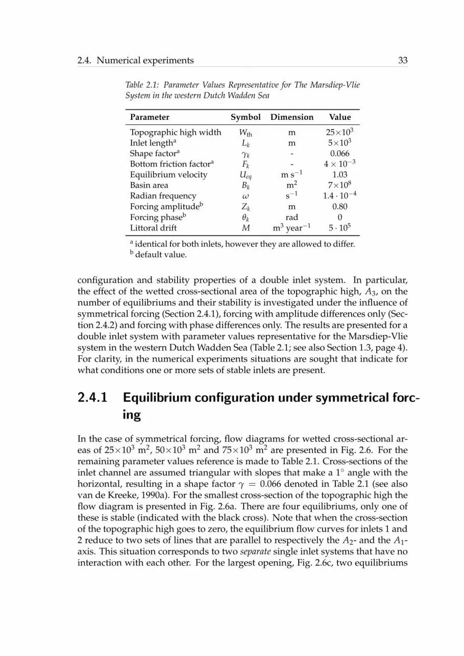
2.4. Numerical experiments 33
Table 2.1: Parameter Values Representative for The Marsdiep-VlieSystem in the western Dutch Wadden Sea
Parameter Symbol Dimension Value
Topographic high width Wth m 25×103
Inlet lengtha Lk m 5×10³
Shape factora γk - 0.066Bottom friction factora Fk - 4× 10⁻³
Equilibrium velocity Ueq m s−1 1.03Basin area Bk m2 7×10⁸
Radian frequency ω s−1 1.4 · 10−4
Forcing amplitudeb Zk m 0.80Forcing phaseb θk rad 0Littoral drift M m3 year−1 5 · 105
a identical for both inlets, however they are allowed to differ.b default value.
configuration and stability properties of a double inlet system. In particular,the effect of the wetted cross-sectional area of the topographic high, A3, on thenumber of equilibriums and their stability is investigated under the influence ofsymmetrical forcing (Section 2.4.1), forcing with amplitude differences only (Sec-tion 2.4.2) and forcing with phase differences only. The results are presented for adouble inlet system with parameter values representative for the Marsdiep-Vliesystem in the western Dutch Wadden Sea (Table 2.1; see also Section 1.3, page 4).For clarity, in the numerical experiments situations are sought that indicate forwhat conditions one or more sets of stable inlets are present.
2.4.1 Equilibrium configuration under symmetrical forc-ing
In the case of symmetrical forcing, flow diagrams for wetted cross-sectional ar-eas of 25×103 m2, 50×103 m2 and 75×103 m2 are presented in Fig. 2.6. For theremaining parameter values reference is made to Table 2.1. Cross-sections of theinlet channel are assumed triangular with slopes that make a 1 angle with thehorizontal, resulting in a shape factor γ = 0.066 denoted in Table 2.1 (see alsovan de Kreeke, 1990a). For the smallest cross-section of the topographic high theflow diagram is presented in Fig. 2.6a. There are four equilibriums, only one ofthese is stable (indicated with the black cross). Note that when the cross-sectionof the topographic high goes to zero, the equilibrium flow curves for inlets 1 and2 reduce to two sets of lines that are parallel to respectively the A2- and the A1-axis. This situation corresponds to two separate single inlet systems that have nointeraction with each other. For the largest opening, Fig. 2.6c, two equilibriums

34 Chapter 2. Influence of a topographic high on cross-sectional inlet stability
0 0.5 1 1.5 20
0.5
1
1.5
2
a) A3= 25×103 [m2]
A1 [×105 m2]
A2 [×
105 m
2 ]
0 0.5 1 1.5 20
0.5
1
1.5
2
b) A3= 50×103 [m2]
A1 [×105 m2]
A2 [×
105 m
2 ]0 0.5 1 1.5 2
0
0.5
1
1.5
2
c) A3= 75×103 [m2]
A1 [×105 m2]
A2 [×
105 m
2 ]
Figure 2.6: Flow diagrams for a double inlet system with a cross-sectional area of the topographichigh of (a) A3 = 25× 103 m2, (b) A3 = 50× 103 m2, and (c) A3 = 75× 103 m2, respectively.The blue and red line correspond to the equilibrium flow curve of Inlet 1 and Inlet 2, respectively.The grey arrows indicate the system’s tendency. The black circles indicate unstable and the blackasterisks indicate stable equilibriums.
exist that are both unstable. The system is reduced to a double inlet system with-out a topographic high. For the flow diagram of the intermediate cross-section,Fig. 2.6b shows that six equilibriums are present, two of which are stable. Toaid the interpretation of this figure, a detailed flow diagram covering the regionincluding the two stable equilibriums in Fig. 2.6b is presented in Fig. 2.7.
The foregoing suggests that depending on the size of the cross-sectional areaof the topographic high there can be one or more stable equilibriums. To preciselyinvestigate the dependency of the number of equilibriums and their stability onthe size of the topographic high, additional calculations were carried out for val-ues of A3 ranging from 20×103 m2 to 80×103 m2 as shown in Fig. 2.8. In thisfigure the cross-sectional area of Inlet 1, A1, is plotted against the cross-sectionalarea of the topographic high, A3. Notice, that a similar figure can be constructedfor the cross-sectional area of Inlet 2. This, however, would not yield additionalinformation because a symmetric double inlet system is assumed, i.e. param-eter values of both inlets are identical. Furthermore, because the interest hereis in the evolution of the stable equilibriums, the unstable equilibrium found inFig. 2.6 close to (A1, A2) = (0, 0) is omitted from this figure. Fig. 2.8 indicatesthat for values of A3 smaller than approximately 30×103 m2 one stable equilib-rium exists (denoted by the blue diamonds). As an example, the black dotted linerepresents the equilibrium configuration of the flow diagram in Fig. 2.6a. Subse-quently, for A3 ranging between approximately 30×103 and 68×103 m2 the num-ber of stable equilibriums increases to two (indicated by the green diamonds).The black dash-dotted line corresponds to the equilibrium configuration foundin Fig. 2.6b. Finally, there are only unstable equilibriums (red diamonds) for val-

2.4. Numerical experiments 35
6 7 8 9 10 116
7
8
9
10
11
A1 [×104 m2]
A2 [×
104 m
2 ]
Figure 2.7: Close-up around the multiple stable equilibriums in Fig. 2.6b. The blue and red linecorrespond to the equilibrium flow curve of Inlet 1 and Inlet 2, respectively. The grey arrowsindicate the system’s tendency. The black circles indicate unstable and the black asterisks indicatestable equilibriums.
ues of A3 larger than 68×103 m2. This situation is exemplified by Fig. 2.6c, whichcorresponds with the black dashed line in Fig. 2.8.
The transition from the situation with two stable equilibriums to the one with-out a stable equilibriums involves the merger of a stable and an unstable equi-librium. The value of A3 associated with this merger is referred to as limit point(LP).
In conclusion, for symmetrical forcing the number of stable equilibriums fora double inlet system with topographic high depends on the size of the wettedcross-sectional area of the topographic high.
2.4.2 Amplitude differences only
To investigate the influence of amplitude differences between the forcing off bothinlets, ∆Z = Z1 − Z2, on the number and stability of equilibriums, Fig. 2.8 hasbeen constructed for amplitude differences ranging between -0.10 m and 0.10m. The result is displayed in Fig. 2.9. In the calculations, Z2 is kept fixed at0.80 m, while Z1 is varied. Other parameter values can be found in Table 2.1.

36 Chapter 2. Influence of a topographic high on cross-sectional inlet stability
2 3 4 5 6 7 80
2
4
6
8
10
12
14
16
LP
LP
A3 [×10
4 m
2]
A1 [
×10
4 m
2]
Figure 2.8: Number of equilibrium cross-sectional areas of Inlet 1 and their stability as a functionof the cross-sectional area of the topographic high for symmetrical forcing. Red diamonds indicateunstable equilibriums, blue diamonds indicate the presence of one set of stable inlets for a certainA3 and green diamonds indicate the presence of two sets of stable inlets for a certain A3. The bluesolid circles denote a limit point, LP, in which a stable and unstable equilibrium merge.
Similarly to the previous section the unstable equilibrium close to (A1, A2) =(0, 0) found in a typical flow diagram is omitted. Notice, when taking a slice ofFig. 2.9 through ∆Z = 0, one would obtain Fig. 2.8. As Fig. 2.9 shows, the numberof stable equilibriums and their stability is, besides the size of the topographichigh, clearly sensitive to the amplitude difference between the forcing off bothinlets.
To enhance the visualisation of Fig. 2.9, sections have been made at A3 =25 × 103 m2 (solid black line), A3 = 50 × 103 m2 (dash-dotted black line) andA3 = 75× 103 m2 (dashed black line). These sections correspond to Figs. 2.10a,2.10b and 2.10c, respectively (see also Fig. 2.6). It follows from Fig.2.10a thatfor the smallest value of the opening over the topographic high (correspond-ing to two separate sub-basins), amplitude differences do not affect the number,nor the stability of the equilibriums. The size of the stable cross-sectional areaof Inlet 1 generally increases for increasingly larger forcing amplitude off thatinlet compared to that off Inlet 2 and vice versa. For the intermediate open-ing, Fig. 2.10b, the number of sets of stable inlets are sensitive to amplitude dif-ferences. In particular, for relatively small values of ∆Z, in this case between

2.4. Numerical experiments 37
2
3
4
5
6
7
8
02
46
810
1214
1618
−0.1
−0.05
0
0.05
0.1
A 3 [×
104 m
2 ]
A1 [×104
m2]
∆ Z
[m]
Figure 2.9: Three-dimensional visualisation of the number of equilibriums and their stability, ex-pressed in terms of A1, as a function of cross-sectional area of the topographic high, A3, and theamplitude difference between the inlet forcings, ∆Z. Red diamonds indicate unstable equilibri-ums, blue diamonds indicate the presence of one set of stable inlets and green diamonds indicatethe presence of two sets of stable inlets for a certain A3-value. The black diamonds indicate theedge of the amplitude difference range at ∆Z = 0.10 m. The black solid, dash-dotted and dashedcross-sections correspond to Figs. 2.10a, 2.10b and 2.10c, respectively.
-0.005 and 0.005 m, two sets of stable inlets exist (indicated by the green dia-monds). For amplitude difference outside this range, the number of sets of stableinlets reduces to one (indicated by the blue diamonds). The maximum range∆Z = [−0.014 m, 0.014 m] was found in Fig. 2.9 at A3 ≈ 65× 103 m2. Finally,Fig. 2.10c indicates that regardless of the amplitude difference, only unstableequilibriums exist for the parameter space investigated here.
To conclude, the results above suggest that the number of sets of stable inletsare only sensitive to amplitude differences for intermediate openings. However,the size of the sets of stable inlets reacts to any change in amplitude difference.

38 Chapter 2. Influence of a topographic high on cross-sectional inlet stability
0 3 6 9 12 15 18−0.1
−0.05
0
0.05
0.1
a) A3=25×103 [m2]
A1 [×104 m2]
∆ Z
[m]
0 3 6 9 12 15 18−0.1
−0.05
0
0.05
0.1
b) A3=50×103 [m2]
A1 [×104 m2]
0 3 6 9 12 15 18−0.1
−0.05
0
0.05
0.1
c) A3=75×103 [m2]
A1 [×104 m2]
Figure 2.10: Cross-sections corresponding to the black solid, dash-dotted and dashed line inFig. 2.9 for (a) A3 = 25× 103 m2, (b) A3 = 50× 103 m2, and (c) A3 = 75× 103 m2. Forreference of the coloured diamonds, see Fig. 2.9.
2.4.3 Phase differences only
Similarly to the previous section, the number of sets of stable inlets is investigatedfor phase difference only, ∆θ = θ1 − θ2, between the forcing off the two inlets.Figs. 2.11 and 2.12 are similarly constructed as Figs. 2.9 and 2.10, respectively. Inthese figures the value of θ2 is kept fixed at zero and θ1 varies between -0.8 and0.8 rad.
The effect of phase difference on the number of sets of stable inlets is similar tothat of amplitude differences. Like amplitude differences, phase differences onlyinfluence the number of sets of stable inlets for intermediate sizes of the openingover the topographic high. For the case displayed in Fig. 2.12b multiple stableequilibriums (indicated by the green diamonds) exist for a range of ∆θ betweenapproximately -0.2 and 0.2 rad. The maximum range ∆θ = [−0.55 rad, 0.55 rad],where two sets of stable inlets exist for a certain value of A3, was found inFig. 2.11 at A3 ≈ 65 × 103 m2. For small openings over the topographic highone set of stable inlets exists (indicated by the blue diamonds). This number isnot affected by phase differences. This also holds for large openings over thetopographic high where no set of stable inlets exists.
To sum up, phase difference affect the number of sets of stable inlets in a sim-ilar manner as amplitude differences: only at intermediate sizes of the openingover the topographic high do they have a significant influence.
2.5 Discussion
For double inlet systems that include a topographic high and are forced by thesame prescribed sea surface elevation off the inlets, results of numerical com-

2.5. Discussion 39
2
3
4
5
6
7
8
02
46
810
1214
1618
−0.8
−0.6
−0.4
−0.2
0
0.2
0.4
0.6
0.8
A 3 [×
104 m
2 ]
A1 [×104
m2]
∆θ [r
ad]
Figure 2.11: Three-dimensional visualisation of the number of sets of stable inlets, expressed interms of A1, as a function of the opening over the topographic high, A3, and the phase differencebetween the forcing off the inlets, ∆θ. Red diamonds indicate the presence of sets of unstable in-lets, blue diamonds indicate the presence of one set of stable inlets and green diamonds indicatethe presence of two sets of stable inlets. The black diamonds indicate the edge of the amplitude dif-ference range at ∆θ = 0.8 rad. The black solid, dash-dotted and dashed cross-sections correspondto Figs. 2.10a, 2.10b and 2.10c, respectively.
putations suggest that there can be more than two equilibriums some of whichare stable. The exact number of equilibriums and their stability, in addition tothe length and friction factor of the inlet channels, strongly depends on the wet-ted cross-sectional area over the topographic high. For a relatively small cross-sectional area, the inlet-bay system behaves as two separate single inlet systems.In that case the two sub-basins act independently and the equilibrium flow curvefor each inlet degenerates to two parallel lines. There are four equilibriums onlyone of which is stable. This result is similar to a two-dimensional representa-tion of the closure curves for single inlet systems introduced by Escoffier (1940)and further investigated and applied to specific sites by O’Brien & Dean (1972);

40 Chapter 2. Influence of a topographic high on cross-sectional inlet stability
0 3 6 9 12 15 18−0.8−0.6−0.4−0.2
00.20.40.60.8
a) A3=25×103 [m2]
A1 [×104 m2]
∆θ [m
]
0 3 6 9 12 15 18−0.8−0.6−0.4−0.2
00.20.40.60.8
b) A3=50×103 [m2]
A1 [×104 m2]
0 3 6 9 12 15 18−0.8−0.6−0.4−0.2
00.20.40.60.8
c) A3=75×103 [m2]
A1 [×104 m2]
Figure 2.12: Cross-sections corresponding to the black solid, dash-dotted and dashed line inFig. 2.11 for (a) A3 = 25 × 103 m2, (b) A3 = 50 × 103 m2, and (c) A3 = 75 × 103 m2.For reference of the coloured diamonds, see Fig. 2.11.
van de Kreeke (1998, 2004). For a large wetted cross-sectional area the inlet baysystem approaches that of the double inlet system without a topographic high.There are at best two equilibriums that both are unstable. This result is in linewith earlier conclusions by van de Kreeke (1985, 1990a,b), who studied the sta-bility of a double inlet system without a topographic high. For the intermediatewetted cross-sectional areas the results become more complex. Depending onthe length, bottom friction factor and shape factor of the inlet channels, therecan be as many as six equilibriums, two of which are stable. The exact causesand conditions that determine the number of stable equilibriums in the case ofan intermediate size wetted cross-section are not clear and are the subject of anongoing study.
As often seen in nature, however, the tides off the various inlets along a bar-rier coast display differences in amplitude as well as in phase. The numericalexperiments in this chapter suggest that amplitude or phase differences influ-ence the equilibrium configuration depending on the size of the topographichigh. For large wetted cross-sectional areas they have no influence: there arestill no stable equilibriums where both inlets are open. Similarly, for small wet-ted cross-sectional areas they do not alter the equilibrium configuration and onestable equilibrium exists. The equilibrium cross-sectional area associated withthe previous two cases, however, does change depending on the amplitude orphase difference. In the case of intermediate wetted cross-sectional areas, eitherone or two stable equilibriums exist. Generally, for relatively small amplitudeor phase differences two stable equilibriums exist and they reduce to one for rel-atively large differences. Unfortunately, exact conditions related to the criticalamplitude or phase difference that indicates the transition between one and twostable equilibriums have not yet been derived and are beyond the scope of this

2.6. Conclusions 41
chapter.In general, it follows that topographic highs can play an important role in the
stability of double inlet systems. A particularly important aspect is that the wa-ter level in the sub-basins, rather than the basin as a whole, fluctuates uniformly.Escoffier (1977) already pointed out that the assumption of the basin surface ele-vation remaining horizontal throughout the tidal cycle is not satisfactory. Basedon observations of seemingly stable multiple inlet systems he further hypothe-sised that spatial variations in the basin could play an important role. This wasalso recognized by Tambroni & Seminara (2006) in their study on the stability ofthe three inlets connecting the Venice Lagoon to the Adriatic Sea. However, theythen proceed in evaluating the stability of the inlets and associated sub-basinsseparately, essentially eliminating the effects of the topographic highs on the sta-bility of the inlets.
A limitation of the modelling approach taken in this chapter is that the forcingoff the inlets has a fixed nature, i.e. they are not influenced by the water motionin the basin nor by interactions between the inlets through the ocean. In reality,however, these mechanism modify the surface elevation off the inlets and there-fore the forcing of the double inlet system. The influence of a dynamical forcingon the cross-sectional stability of double inlet systems will be discussed in moredetail in Chapter 4.
2.6 Conclusions
The equilibrium configurations and stability properties of double inlet systemswith a topographic high in the basin are investigated using the results of nu-merical experiments. In addition, the sensitivity of the number and stability ofequilibrium cross-sections is investigated with respect to amplitude or phase dif-ferences between the forcing off the two inlets.
The suggestion in the Introduction of this chapter that a topographic highdividing the basin in two sub-basins plays a role in the stability of the inlets isconfirmed by the numerical experiments. In the presence of a topographic highthe water level in the sub-basins, rather than in the basin as a whole, fluctuatesuniformly.
For a small cross-sectional area of the topographic high the system is reducedto two separate single inlet systems. There are four equilibriums, one of whichis stable with two inlets open. Amplitude or phase differences do not affect thenumber nor the stability of the equilibriums within the investigated parameterspace.
For a large cross-sectional area the system approaches a double inlet systemwithout a topographic high. Assuming entrance/exit losses can be neglected,at best there are two equilibriums neither of which is stable. Similar to smallcross-sectional areas amplitude or phase differences do not affect the stability

42 Chapter 2. Influence of a topographic high on cross-sectional inlet stability
configuration.In the transition region between small and large cross-sectional areas of the
topographic high as many as six equilibriums can exist. The number of stableequilibriums is sensitive to the amplitude or phase difference between the forc-ing off the two inlets. For relatively small amplitude or phase differences, twostable equilibriums are present with two inlets open. It was found in this chapterthat, for the parameter space investigated, the maximum amplitude and phaserange where two stable equilibriums are present, is ∆Z ≈ [−0.014 m, 0.014 m]and ∆θ ≈ [−0.55 rad, 0.55 rad], respectively. The exact range depends, amongstothers, on the size of the topographic high. Outside those ranges the number ofstable equilibriums with two inlets open is reduced to one.

2.A. Solution method double inlet system with topographic high 43
2.A Solution method double inlet system withtopographic high
To solve the non-linear system of equations (2.11)-(2.13) introduced in section 2.3,use is made of the Newton-Raphson method. As a first step, the system of equa-tions is written in matrix notation. For convenience, the governing equations(2.11)-(2.13) are rearranged and repeated here. Continuity gives:
Bkdζbk
dt= Akuk + (−1)k A3u3, k = 1, 2, (2.A.1)
and momentum conservation gives:
RkFk
dukdt
+ |uk|uk = Γk(ζk − ζbk
), k = 1, 2, (2.A.2)
R3
F3
du3
dt+ |u3|u3 = Γ3
(ζb1 − ζb2
), (2.A.3)
where Rk = γ√
Ak (k = 1, 2), R3 = A3/Wth and
Γk =
gRkFkLk
, k = 1, 2,
Γ3 =gA3
F3L3Wth.
(2.A.4)
An explanation of the symbols throughout this appendix is given in section 2.3.The external forcing is defined as
ζk = <
ζkeiωt
, with ζk = Zkeiθk and k = 1, 2, (2.A.5)
where ζk is the complex amplitude of the water elevation. Consequently, ap-proximate periodic solutions are sought, whereby a trial solution is assumed ofthe form
uk = <
ukeiωt
, k = 1, 2, 3, (2.A.6)
where uk is the complex amplitude of the inlet velocities and the velocity overthe topographic high. The Galerkin technique (see e.g. Boyd, 2001) is used to

44 Chapter 2. Influence of a topographic high on cross-sectional inlet stability
make an estimation of the amplitudes that correspond to the trial solution (2.A.6).Substitution of Eq. (2.A.6) into the continuity equation yields
ζbk=
1iω
(AkBk
uk + (−1)k A3
Bku3
). (2.A.7)
Combining (2.A.5)-(2.A.7) with momentum conservation (2.A.2) and (2.A.3) yieldsfor the tidal inlets
(−βk + i|uk|) uk + (−1)kηku3 = iΓk ζk, (2.A.8)
and for the topographic high
−τ1u1 + τ2u2 + β3u3 + i|u3|u3 = 0, (2.A.9)
Here,
βk = ω
RkFk− 1
ωΓk
AkBk
, k = 1, 2,
β3 = ωR3
F3− 1
ωΓ3
(A3
B1+
A3
B2
),
(2.A.10)
and
ηk =1ω
ΓkA3
Bk, (2.A.11)
τk =1ω
Γ3AkBk
(2.A.12)
Separating Eqs. (2.A.8) and (2.A.9) into real and imaginary parts and definingζk = ζc,k + iζs,k and uk = uc,k + ius,k yields for the inlets
< : −βkuc,k − |uk|us,k + (−1)kηkuc,3 = −Γkζs,k,
= : −βkus,k + |uk|uc,k + (−1)kηkus,3 = Γkζc,k,(2.A.13)
and for the topographic high
< : −τ1uc,1 + τ2uc,2 − β3uc,3 − |u3|us,3 = 0,= : −τ1us,1 + τ2us,2 − β3us,3 + |u3|uc,3 = 0.
(2.A.14)

2.A. Solution method double inlet system with topographic high 45
In these equations |uk| = 2π
√u2
c,k + u2s,k, in accordance with the Galerkin method.
For convenience, the system above is written in matrix notation
|u1| −β1 0 0 0 −η1−β1 −|u1| 0 0 −η1 0
0 0 |u2| −β2 0 −η20 0 −β2 −|u2| −η2 00 −τ1 0 τ2 |u3| −β3−τ1 0 τ2 0 −β3 −|u3|
uc,1us,1uc,2us,2uc,3us,3
=
Γ1ζc,1−Γ1ζs,1Γ2ζc,2−Γ2ζs,2
00
, (2.A.15)
or in short form
M · x = b (2.A.16)
This system can be solved numerically using the Newton-Raphson method (seee.g. Abramowitz & Stegun, 1972), which holds the following. Eq. (2.A.16) can bewritten as
f (x) = b. (2.A.17)
Defining a new function g(x),
g(x) = f (x)− b = 0, (2.A.18)
a solution x∗ is sought for the above equations g. With the Newton-Raphsonmethod g is approximated with a first order Taylor polynomial, according to
g(x∗ + ∆x) = g(x∗) +n
∑j=1
∆xj∂gj(x)
∂xj
∣∣∣∣∣x∗
, (2.A.19)
where n = 6 for this particular case. Assume that x + ∆x = x∗. In that case
g(x) +n
∑j=1
∆xj∂gj(x)
∂xj
∣∣∣∣∣x∗
= 0, (2.A.20)
or
n
∑j=1
∆xj∂gj(x)
∂xj
∣∣∣∣∣x∗
= −g(x∗). (2.A.21)

46 Chapter 2. Influence of a topographic high on cross-sectional inlet stability
This latter system is linear in ∆x. In short matrix notation this can be written asY·∆x = −g(x∗), or
∂g1∂x1
∣∣∣x∗
. . . ∂g1∂xn
∣∣∣x∗
... . . . ...∂gn∂x1
∣∣∣x∗
. . . ∂gn∂xn
∣∣∣x∗
∆x1
...∆xn
= −
g1(x∗)...
gn(x∗)
. (2.A.22)
From this the ∆x can be determined. Consequently, they are used to obtain thex∗ via iteration. An approximated x is adjusted to a new (better) approxima-tion x + ∆x = x∗, using ∆x derived from matrix (2.A.22). It turns out that witha reasonable first estimate of x this method converges relatively fast. From theconverged solution x the amplitude of the inlet velocities can be calculated ac-
cording to Uk =√
u2c,k + u2
sk. In turn, Uk is used to construct the flow diagram
from which the cross-sectional stability can be assessed.


3Entrance/exit losses and
cross-sectional inletstability*
Abstract In this chapter the effect of entrance/exit losses on the cross-sectionalstability of double inlet systems is investigated. The inlet is in equilibrium whenthe sand transport into the inlet equals the sand transport out of the inlet. Thevelocity amplitude corresponding with the equilibrium cross-sectional area isreferred to as the equilibrium velocity (∼1 m s−1). This equilibrium is stablewhen after a perturbation the cross-sections of both inlets return to their origi-nal equilibrium values. The amplitudes of the inlet velocities are obtained usinga lumped-parameter model in which the basin water level fluctuates uniformly(pumping mode) and where the inlets are schematised to prismatic channels. Thesystem is forced by a semi-diurnal tide, where amplitude and phase may differbetween the two inlets. Previous studies concluded that for double inlet systemsno stable equilibriums can be found. However, in these studies entrance/exitlosses were neglected. In the present study entrance/exit losses are included inthe dynamic equation of the inlets.
Using an analytical model it is shown that entrance/exit losses and a differ-ence in the two ocean tidal amplitudes are a prerequisite for the existence of sta-ble equilibriums. Furthermore, the effects of the addition of bottom friction andinertia to the dynamic equation are investigated using a mathematical continu-
*This chapter has appeared as ”Entrance/exit losses and cross-sectional stability of double inletsystems” by R.L. Brouwer, J. van de Kreeke and H.M. Schuttelaars (2012), Est. Coast. Shelf Sci.107, pp. 69-80.
49

50 Chapter 3. Entrance/exit losses and cross-sectional inlet stability
ation method. The results show that, provided entrance/exit losses are consid-erably larger than bottom friction and inertia, stable equilibriums are possible.These conclusions are supported by observations in the Ria Formosa, southernPortugal. Care should be taken in using the stability model described in this pa-per as a predictive tool due to simplifications in the model and the uncertainty indetermining certain parameter values including inlet length, entrance/exit losscoefficient, bottom friction factor and equilibrium velocity. To alleviate theseshortcomings suggestions are made for future research.
3.1 Introduction
Barrier island coasts are highly dynamical systems that serve as a first defencefor the hinterlying mainland. Examples are the Wadden Sea coast of the Nether-lands, Germany and Denmark (Ehlers, 1988), the U.S. part of the Gulf of Mexico,the U.S. East Coast and Ria Formosa in Southern Portugal. These barrier islandcoasts are a concatenation of tidal inlet systems, in which a tidal basin or back-barrier area is connected to the ocean or sea by one or more tidal inlets.
Tidal inlet systems in sandy environments consist of different elements in-cluding ebb tidal delta, inlet channel and basin. Restricting attention to inletswhere river flow has a minor impact, the dimensions of the various elementsare a result of primarily tide and waves. The interest here is in the equilibriumand stability of the cross-sectional area of the inlet channel; the channel connect-ing ocean and basin. Referring to Escoffier (1940) the cross-sectional area of atidal inlet takes on a value such that the wave-driven sediment import equalsthe tide-driven sediment export. The velocity amplitude corresponding with theequilibrium cross-sectional area is referred to as the equilibrium velocity. Basedon observations Escoffier suggested an approximate value of 1 m s−1, the ex-act value depending somewhat on the volume of littoral drift. The actual cross-sectional area oscillates around this equilibrium value. By opening a new inlet oras a result of land reclamation the deviation from the equilibrium value can be-come so large that the cross-sectional stability is challenged and one of the inletsmay close. It is therefore of importance to assess if and under what conditionsstable equilibrium configurations of multiple tidal inlet systems are expected toexist.
As a first step to investigate multiple tidal inlet stability, van de Kreeke (1985,1990a) studied the stability of a double inlet system. He used a L-P model todescribe the hydrodynamics of the system. Similar to Keulegan (1951), van deKreeke simplified the dynamic equation of the L-P model by only retaining thequadratic bottom friction and pressure gradient while neglecting inertia and en-trance/exit losses. The double inlet system was assumed to be in equilibriumif the velocity amplitude in the inlets equals the equilibrium velocity taken as 1m s−1. The forcing off the two inlets consisted of a simple harmonic tide with

3.1. Introduction 51
equal amplitude and phase. The main conclusion was that for these conditionsno stable equilibrium(s) exist, i.e. ultimately one of the inlets would close. Fur-thermore, he suggested that a similar conclusion holds for multiple inlet systems.
Several observations, however, have shown that multiple inlet systems arepotentially stable for over several centuries. Examples are Gasparilla Sound inwestern Florida (Escoffier, 1977), the Dutch Wadden Sea (Louters & Gerritsen,1994) and Rıa Formosa in southern Portugal (Salles et al., 2005; Pacheco et al.,2010, 2011a). These observations suggest that the assumptions of the hydrody-namic model used by van de Kreeke (1985, 1990a) might be too restrictive and donot take into account important (non-linear) processes, such as tidal distortion inthe basin (e.g. Boon & Byrne, 1981). To overcome these restrictions, one approachis to use state of the art process-based models describing the complex flow field(e.g. Salles et al., 2005; Dias & Sousa, 2009) and resulting sediment transport andbottom changes (e.g Dastgheib et al., 2008). As discussed in the introduction ofthis thesis, one of the drawbacks of these models is that due to their complexity itis difficult to determine cause and effect. Consequently, insight into the physicalmechanisms responsible for the existence of stable tidal inlet systems with morethan one inlet open is difficult to ascertain.
Another approach is to parameterise the important processes into the L-Pmodel. An advantage of this approach is that it facilitates analytical solutionmethods to determine which underlying mechanisms are important for the sta-bility of tidal inlet systems. Support for the use of this type of model has beenprovided by Herman (2007), who compared the results of a 2D finite differencehydrodynamic model and a L-P model. The results show that the L-P modelcaptures the important dynamics of the inlet flow.
In this chapter, the latter L-P model is used to investigate recent observationsin the multiple inlet system of Rıa Formosa (Pacheco et al., 2010, 2011a), whichhas persisted on a historical time scale (see also Section 1.3 on page 4). In particu-lar the sub-system consisting of the two inlets Faro and Armona and connectinga single basin to the ocean can be considered in stable equilibrium. A characteris-tic for this double inlet system is that the inlets are relatively short and thereforeentrance/exit losses are not necessarily small compared to bottom friction losses.This loss-term was neglected in the study by van de Kreeke (1990a). The objec-tive of this chapter is to investigate the role of the different terms in the L-P modelon cross-sectional stability of double inlet systems with special reference to theentrance/exit loss term.
This chapter is organised as follows. In Section 3.2, the governing equationsof a double inlet system are presented. In addition, a new visualisation methodto analyse the influence of the different terms in the dynamic equation on theequilibrium and stability of double inlet systems is introduced. Section 3.3 con-tains the derivation of the necessary conditions for stable double inlet systemsto exist when only entrance/exit losses balance the pressure gradient over theinlets. Subsequently, in Section 3.4 the addition of bottom friction and inertia

52 Chapter 3. Entrance/exit losses and cross-sectional inlet stability
ζb, B
u1(A
1,A
2)
ζ1
u2(A
1,A
2)
ζ2
L
M
Figure 3.1: Schematisation of a double inlet system draining a single basin. For an explanationof the symbols, see Subsection 3.2.1.
on the equilibrium and stability is investigated. In Section 3.5, the effect of forc-ing on stable equilibriums is looked into. The results and insights obtained fromthe previous section are then applied to the Faro-Armona double inlet system inSection 3.6. Finally, Sections 3.7 and 3.8 present the discussion and conclusions,respectively.
3.2 Governing equations and method
3.2.1 Governing Equations
In this chapter the double inlet system is schematised to a single basin connectedto the sea or ocean by two tidal inlets (Fig. 3.1). The basin is relatively smalland deep and the tidal inlets are prismatic channels with diverging sections oneither end. The focus is on cross-sectional stability. Following Escoffier (1940) aninlet is in equilibrium if the amplitude of the inlet velocity equals the so-calledequilibrium velocity Ueq. Escoffier suggested this velocity to be of the order of

3.2. Governing equations and method 53
1 m s−1. The equilibrium is stable when after a perturbation of the equilibrium,the cross-sectional areas return to their original equilibrium values.
For inlets that are in equilibrium and assuming average weather conditions(as opposed to storm conditions) there is a balance between the volume of sedi-ment entering and leaving the inlet. The volume entering the inlet is taken as aconstant fraction of the littoral drift and the volume leaving the inlet is taken pro-portional to a power of the ebb tidal velocity amplitude (van de Kreeke, 1998).The sediment is uniformly distributed over the inlet length and sediment ex-change between inlet and basin is assumed to be negligible. Under these as-sumptions, the rate of change of the cross-sectional area can be written as (van deKreeke, 1998)
dAkdt
=ML
[(UkUeq
)n− 1]
, k = 1, 2. (3.1)
Here, Ak is the cross-sectional area of inlet k (m2); t is time (s); L is the inletlength (m); M is a constant fraction of the littoral drift (m3 s−1); Uk is the cross-sectionally averaged velocity amplitude in inlet k (m s−1), calculated using theL-P model; Ueq is the equilibrium velocity (m s−1). If the inlet velocity Uk equalsUeq, dAk/dt = 0. This implies that the inlet system is in equilibrium. n is apower whose value depends on the adopted sand transport law. Values of nrange between 3 and 6 (van Rijn, 1993). The value of n influences the direction ofthe unit vectors in the flow diagram, Fig. 3.2 (see also Section 2.2 on page 24). Thedirection of these vectors in the neighbourhood of the equilibrium determineswhether the equilibrium is stable or unstable. However, linearising Eq. (3.1) itcan be shown that in the neighbourhood of the equilibrium the direction of theseunit vectors become independent of n. Therefore, the value of n does not playa role in the stability of the equilibrium. In the calculations n was somewhatarbitrarily given a value of 3.
The response of the inlet cross-sectional area and the equilibrium state is gov-erned by the amplitude of the inlet velocities Uk. These velocities are calculatedusing a L-P model. In this model the dynamics of the flow in the diverging sec-tions is governed by the advective acceleration and the longitudinal pressuregradient (see Vennell, 2006, for support of this governing balance by ADCP mea-surements in a tidal inlet connecting Tauranga Harbour to the Pacific Ocean, NewZealand). Energy losses in these sections are taken as a fraction of the velocityhead. The dynamics of the flow in the prismatic section constitutes a balance be-tween longitudinal pressure gradient, inertia and bottom friction. The resultingequation is
Lg
dukdt
+8
3π
(m2g
+FLgRk
)Ukuk = ζk − ζb, k = 1, 2. (3.2)

54 Chapter 3. Entrance/exit losses and cross-sectional inlet stability
Here g ≈ 9.81 m s−2 the gravitational acceleration; uk denotes the cross-sectionallyaveraged velocity in inlet k (m s−1); m the entrance/exit loss coefficient (-); F thedimensionless bottom friction factor (-); Rk the hydraulic radius of inlet k (m); ζkthe sea surface elevation off inlet k (m); and ζb the basin surface level elevation(m) (where ζb = 0 corresponds to mean sea level). The quadratic term |uk|uk inEq. (3.2) is linearised and replaced by (8/(3π))Ukuk, with Uk = Ueq (see Lorentz,1926; Zimmerman, 1982). The reason to do so is that this linearisation is neces-sary for the solution method described in Section 3.2.2. Moreover, the results inthe neighbourhood of the equilibrium are not affected by this linearisation.
Because the basin is assumed to be relatively small and deep the water level toa good approximation fluctuates uniformly (pumping mode) and the continuityequation reads
Bdζbdt
= A1u1 + A2u2, (3.3)
in which B is the basin surface area (m2).Eqs. (3.2) and (3.3) constitute a L-P model. For a single inlet system the first
order analytical solution for u and ζb are functions of two dimensionless param-eters involving ζ0, L, A, F, m and B, hence the designation lumped-parameter(L-P) model. For a detailed derivation of Eqs. (3.2) and (3.3) reference is made toMehta & Ozsoy (1978) and van de Kreeke (1988). Another approach that leads toa similar momentum equation as Eq. (3.2) is presented by Maas (1997).
In most studies the entrance/exit loss coefficient m is assumed to be 1 (e.g.O’Brien & Clark, 1974; Escoffier, 1977; Tambroni & Seminara, 2006). Other stud-ies give a specific range for m: e.g. van de Kreeke (1988) suggests a range between0.3 and 1.4 and Seabergh (2002) adopts a range of m between 1 and 1.25. Theo-retically the value of m cannot be larger than 2. In the literature values of F rangebetween 2 · 10−3 and 4 · 10−3. With m = O(1) and F = O(10−3) it follows thatthe entrance/exit loss term and bottom friction term in Eq. (3.2) are of the sameorder for L/R = 500. With a typical value R = 5 m for tidal inlets, L = 2500 m.For values of L < 2500 m the entrance/exit loss term is more important than thebottom friction term and for L > 2500 m the entrance/exit loss term is less impor-tant than the bottom friction term. For L = 2500 m and a semi-diurnal tide, withω = 1.4 · 10−4 s−1, the inertia term is approximately half of the entrance/exitloss term. This suggests that for relatively short tidal inlets, entrance/exit lossescannot be neglected.
In addition, from Eq. (3.1) a time scale for coastal evolution can be deduced.Assuming the term between square brackets on the right-hand side is O(1), thetime scale T = AL/M. For relatively short inlets, with L = O(103), A = O(103)and M = O(105), the time scale is in the order of decades. For relatively longinlets, with L = O(103), A = O(105) and M = O(106), the time scale is in theorder of centuries. It follows that the time scale for coastal evolution for tidal

3.2. Governing equations and method 55
inlet systems is in the order from decades to centuries.To relate the hydraulic radius Rk to the cross-sectional area, the cross-sections
are assumed to be geometrically similar for all values of the cross-sectional area(following O’Brien & Dean, 1972). Hence, the ratio of all corresponding lengthsfor two cross-sections are the same. This allows writing
Rk = γ√
Ak, (3.4)
where γ is a shape factor (-), which is assumed to be constant.The tidal motion in the inlets is forced by a semi-diurnal harmonic constituent,
where amplitudes and phases may differ between the two inlets,
ζk = <
Zkei[ωt+θk]
. (3.5)
Here < denotes the real part, Zk is the real-valued amplitude of the ocean tideat inlet k (m) and θk the phase of the ocean tide at inlet k (rad). Note that theamplitude and phase of the forcing off the inlets are fixed and not dynamic, i.e.they are not influenced by dynamic interactions with the basin.
3.2.2 Methods
Flow Diagram
To determine the equilibrium cross-sectional areas and their stability use is madeof a so-called flow diagram. For a detailed description on how to construct sucha flow diagram, the reader is referred to Section 2.2 on page 24. An example ofa flow diagram, using the parameter values of Table 3.1, is presented in Fig. 3.2.These parameter values pertain to a symmetric double inlet system, i.e. L, F, mand γ for both inlets are the same, resembling the Faro-Armona system, whereInlet 1 refers to Armona and Inlet 2 refers to Faro. The reason a symmetric inletsystem is selected is to facilitate a physical explanation for the role of the en-trance/exit losses in the cross-sectional stability of a double inlet system. Thereal Faro-Armona system is not symmetric and a detailed description includ-ing parameter values for this system is presented in Section 3.6. In constructingthe flow diagram use is made of a numerical solution to Eqs. (3.2)-(3.5). Fromthis, equilibrium velocity curves are constructed for both inlets. The equilibriumvelocity curves represent the locus of (A1, A2)-values for which U1 = Ueq andU2 = Ueq. The intersections of the two curves represent sets of equilibrium cross-sectional areas. To determine the stability of the equilibrium, vectors are addedto the flow diagram. These vectors are the unit vectors in the direction of d~A/dtcalculated from Eq. (3.1). The unit vectors indicate the direction in which the val-ues of cross-sectional areas change when they are not in equilibrium. Using this

56 Chapter 3. Entrance/exit losses and cross-sectional inlet stability
Table 3.1: Parameter Values for a symmetric double inlet system resembling the Faro-Armona system
Parameter Symbol Dimension Value Inlet 1 Value Inlet 2(Armona) (Faro)
InletsInlet cross-section Ak m2 variable variableInlet length Lk km 1 1Entrance/exit coefficient mk - 1 1Inlet shape factor γk - 0.2 0.2Friction factor Fk - 2× 10⁻³ 2× 10⁻³
Equilibrium velocity Ueq m s−1 1 1ForcingRadian frequency ω* s−1 1.4× 10⁻⁴
Sea surface amplitude Zk m 1.43 1.36Sea surface phase θk rad 0 0GeneralBasin surface area B* m2 3.4× 10⁷
Sediment import M* m3 year−1 1× 10⁵
* pertaining to the entire system
information, the black circles represent unstable equilibriums and the black crossrepresents a stable one.
Continuation Method
Even though a flow diagram is a useful tool to assess cross-sectional stability, itdoes not provide direct insight in the effect of individual terms on the dynamicequation and the various parameters, e.g. L, m, F, γ, Zk and θk (k = 1, 2), on thepresence of equilibriums. To investigate these effects a mathematical continuationmethod (CL MATCONT; Dhooge et al., 2003) is used.
As an example of the use of this method and the presentation of the results,the influence of the inlet length L on the stable equilibrium in Fig. 3.2 is shownin Fig. 3.3. Starting with a known equilibrium solution (Aeq
1 , Aeq2 ), e.g. the sta-
ble equilibrium denoted with the black cross in Fig. 3.2, the parameter value Lis slightly decreased or increased by CL MATCONT and a new equilibrium so-lution is calculated. The continuation method assesses the local stability of thisequilibrium by conducting a linear stability analysis. Repeating the procedure,a curve with equilibrium values (Aeq
1 , Aeq2 ) as a function of L is found depicted
in Fig. 3.3a. For reference the flow diagram of Fig. 3.2 pertaining to L = 1 km isadded to Fig. 3.3a to show how the cyan curve in this figure is related to the equi-librium velocity curves in the flow diagram. This clearly shows that the unstablebranch of the cyan curve passes through the flow diagram at an unstable equilib-

3.2. Governing equations and method 57
2 4 6 8
2
4
6
8
A1 [×103 m2]
A2 [×
103 m
2 ]
Figure 3.2: Flow diagram with parameters resembling the Faro-Armona system. The blue and redsolid line correspond to the equilibrium flow curves of Inlet 1 and 2, respectively, the grey vectorsindicate the direction in which the values of the cross-sectional areas change when they are notin equilibrium, the black circles indicate an unstable equilibrium and the black cross indicates astable equilibrium. Calculations carried out using Eq. (3.2); m = 1, γ = 0.2, F = 2 · 10−3,L = 1 km, Z1 = 1.43 m, Z2 = 1.36 m, θk = 0 (k = 1, 2).
rium (indicated by a black circle) and the stable branch passes through the flowdiagram at a stable equilibrium (indicated by a black cross). Inspection with thecontinuation method of the other two unstable equilibriums found in the flowdiagram showed that they remain unstable for the parameter space inspectedhere. Because the interest is in stable equilibriums, their dependence on L is notshown. The maximum inlet length for which a stable equilibrium exists is foundat the point indicated by the black dot denoted as LP. Here, LP stands for LimitPoint, which means that the stability of the equilibrium changes from stable tounstable, or vice versa, when crossing this point on the cyan curve. Furthermore,the cyan curve and the black markers are projected on the (A1, A2)-plane in greyto help visualize the path of the cyan curve and the location of the markers.
When projecting the curve on the (L, Ak)-plane, with k = 1, 2, Fig. 3.3b isobtained. In contrast to Fig. 3.3a, this figure more clearly shows that there is amaximum L for which a stable equilibrium exists.

58 Chapter 3. Entrance/exit losses and cross-sectional inlet stability
02
46
8
02
46
80
0.5
1
1.5
A1 [×103 m2]
a) (A1eq,A
2eq) vs. inlet length
LP
A2 [×103 m2]
L [k
m]
0 0.25 0.5 0.75 1 1.25 1.50
2
4
6
8
LPA
2
LPA
1
b) 2D projection of (A1eq,A
2eq)
L [km]A
k [×10
3 m2 ] (
k=1,
2)
Figure 3.3: Visualizing the influence of parameter variability on the stability of an equilibrium.(a) (Aeq
1 , Aeq2 ) for a tidal inlet system resembling the Faro-Armona (in cyan), for varying inlet
length L. The dashed, cyan line indicates linearly unstable solutions (unstable saddle) and thesolid, cyan line indicates linearly stable solutions (stable node). The cyan curve passes throughthe flow diagram at the black circle, indicating an unstable equilibrium, and at the black cross, in-dicating a stable equilibrium. The black dot indicates a limit point, where the cyan curve changesstability. The cyan curve and the black markers are projected on the base plane in grey. (b) Pro-jection of (Aeq
1 , Aeq2 ) in (a) on the (L, Ak)-plane (k = 1, 2). The blue line corresponds to Inlet 1
and the red line to Inlet 2. A solid line indicates stable equilibriums and a dashed line unstableones. Calculations carried out using Eq. (3.2); m = 1, γ = 0.2, F = 2 · 10−3, Z1 = 1.43 m,Z2 = 1.36 m, θk = 0 (k = 1, 2).
3.3 Entrance/exit losses only
3.3.1 Conditions for stable equilibriums
Neglecting inertia and bottom friction in the dynamic equations, Eq. (3.2), andtaking Uk = Ueq, yields
cmUequk = ζk − ζb, with c = 43πg . (3.6)
In a strict sense, when replacing Uk with Ueq in the linearised quadratic term,Eq. (3.6) is only valid in a neighbourhood of the equilibrium. Solutions to Eq. (3.6)and the continuity equation Eq. (3.3) are presented in Appendix 3.A.1. In this ap-pendix, the forcing condition ζk = Zk exp(iωt) is used, where only amplitudedifferences between the inlets are allowed so that an analytical approach is pos-sible. At the end of this section the case of only phase differences between the in-

3.3. Entrance/exit losses only 59
lets is briefly discussed. Because of its importance in determining cross-sectionalstability the solution for Uk is repeated here:
Uk =1
cmUeq
√(µmUeqZk)2 + A2
3−k(Z1 − Z2)2
(µmUeq)2 + (A1 + A2)2 , (3.7)
where µ = cωB. For equilibrium, the inlet velocities U1 and U2 must be equalto the equilibrium velocity Ueq. This results in a system of two equations in A1and A2 from which in principle the conditions for equilibrium can be derived.Two cases can be distinguished, equal amplitudes of the sea surface elevation(Z1 = Z2) and different amplitudes (Z1 6= Z2).
For Z1 = Z2 = Z0 there is an infinite number of equilibriums:
Aeq1 + Aeq
2 =µmUeq
√Z2
0(cm)2 −U4
eq. (3.8)
This is a straight line of equilibrium points in the (A1, A2)-space. Eq. (3.8) is onlyvalid if the argument under the square root is positive, i.e. Z0 > cmU2
eq. Froma linear stability analysis (see 3.C) it follows that the equilibriums are alwaysneutrally stable, which means that when an arbitrary equilibrium is perturbed itwill return to an equilibrium, however, not necessarily the same one. In nature,this situation is not often encountered, as usually the amplitudes off the inletsdiffer.
In case of Z1 6= Z2 conditions under which equilibriums exist are difficultto derive directly from Eq. (3.7). Therefore, a slightly different approach is taken;see Appendix 3.A.2. From this the following expression for the equilibrium cross-sectional areas is derived:
Aeqk =
µmsin ψ
eq1
[Z1 + Z2
4cmUeq− (−1)kUeq
(1− cos2 ψ
eq1
2 cos ψeq1
)], k = 1, 2, (3.9)
where
cos ψeq1 =
∆Z2cmU2
eq. (3.10)
Here, ψ1 is the phase of the inlet velocity in inlet 1 and ∆Z = Z1 − Z2. For Aeq1
and Aeq2 to be positive it follows from Eq. (3.9) that
Z1∆Z2(cm)2U4
eq≥ 1, ∆Z > 0. (3.11)

60 Chapter 3. Entrance/exit losses and cross-sectional inlet stability
Table 3.2: Conditions for Equilibrium Cross-Sectional Areas to Exist and Stability Modes; En-trance/Exit Losses Only
Amplitude Number of Equilibriums Stability Mode
Z1 = Z2 = Z0 Infinite, provided Z0 > cmU2eq Neutrally Stable
∆Z > 0
1, provided2(cm)2U4
eqZ1
≤ ∆Z ≤ 2cmU2eq Stable
0 in all other cases than above
∆Z < 0
1, provided2(cm)2U4
eqZ2
≤ −∆Z ≤ 2cmU2eq Stable
0 in all other cases than above
From Eq. (3.10) with | cos ψ1| ≤ 1, it follows that
∆Z2cmU2
eq≤ 1, ∆Z > 0. (3.12)
Similar conditions as those given by Eqs. (3.11) and (3.12) hold for ∆Z < 0. Inthat case, Z1 is replaced by Z2 in Eq. (3.11) and in Eqs. (3.11) and (3.12) ∆Z isreplaced by −∆Z. From Eqs. (3.11) and (3.12) it follows that there is a limitedinterval of m-values for which equilibriums exist. The interval ranges from mminto mmax with
mmin =∆Z
2cU2eq
, (3.13)
and
mmax =1
cU2eq
√Z1∆Z
2. (3.14)
It can be shown that the equilibriums in this interval are linearly stable (see Ap-pendix 3.C). In Table 3.2 an overview is given of the conditions for equilibriumfor both Z1 = Z2 and Z1 6= Z2. In the same table their linear stability is indicated.
3.3.2 Physical explanation for the interval of stableequilibriums when Z1 6= Z2
In the foregoing it is shown that for mmin ≤ m ≤ mmax (physically realistic) sta-ble equilibriums exist, i.e. the amplitude of the velocity in both inlets equals theequilibrium velocity. Given a value of m, inlet velocities depend on the differencein water level between basin and ocean. A logical question then is what are theamplitude and phase of the basin water level at times of equilibrium and how dothey depend on the entrance/exit loss coefficient m?
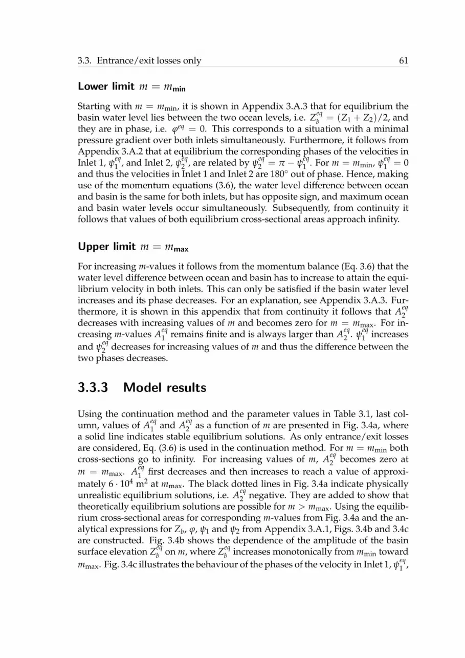
3.3. Entrance/exit losses only 61
Lower limit m = mmin
Starting with m = mmin, it is shown in Appendix 3.A.3 that for equilibrium thebasin water level lies between the two ocean levels, i.e. Zeq
b = (Z1 + Z2)/2, andthey are in phase, i.e. ϕeq = 0. This corresponds to a situation with a minimalpressure gradient over both inlets simultaneously. Furthermore, it follows fromAppendix 3.A.2 that at equilibrium the corresponding phases of the velocities inInlet 1, ψ
eq1 , and Inlet 2, ψ
eq2 , are related by ψ
eq2 = π − ψ
eq1 . For m = mmin, ψ
eq1 = 0
and thus the velocities in Inlet 1 and Inlet 2 are 180 out of phase. Hence, makinguse of the momentum equations (3.6), the water level difference between oceanand basin is the same for both inlets, but has opposite sign, and maximum oceanand basin water levels occur simultaneously. Subsequently, from continuity itfollows that values of both equilibrium cross-sectional areas approach infinity.
Upper limit m = mmax
For increasing m-values it follows from the momentum balance (Eq. 3.6) that thewater level difference between ocean and basin has to increase to attain the equi-librium velocity in both inlets. This can only be satisfied if the basin water levelincreases and its phase decreases. For an explanation, see Appendix 3.A.3. Fur-thermore, it is shown in this appendix that from continuity it follows that Aeq
2decreases with increasing values of m and becomes zero for m = mmax. For in-creasing m-values Aeq
1 remains finite and is always larger than Aeq2 . ψ
eq1 increases
and ψeq2 decreases for increasing values of m and thus the difference between the
two phases decreases.
3.3.3 Model results
Using the continuation method and the parameter values in Table 3.1, last col-umn, values of Aeq
1 and Aeq2 as a function of m are presented in Fig. 3.4a, where
a solid line indicates stable equilibrium solutions. As only entrance/exit lossesare considered, Eq. (3.6) is used in the continuation method. For m = mmin bothcross-sections go to infinity. For increasing values of m, Aeq
2 becomes zero atm = mmax. Aeq
1 first decreases and then increases to reach a value of approxi-mately 6 · 104 m2 at mmax. The black dotted lines in Fig. 3.4a indicate physicallyunrealistic equilibrium solutions, i.e. Aeq
2 negative. They are added to show thattheoretically equilibrium solutions are possible for m > mmax. Using the equilib-rium cross-sectional areas for corresponding m-values from Fig. 3.4a and the an-alytical expressions for Zb, ϕ, ψ1 and ψ2 from Appendix 3.A.1, Figs. 3.4b and 3.4care constructed. Fig. 3.4b shows the dependence of the amplitude of the basinsurface elevation Zeq
b on m, where Zeqb increases monotonically from mmin toward
mmax. Fig. 3.4c illustrates the behaviour of the phases of the velocity in Inlet 1, ψeq1 ,

62 Chapter 3. Entrance/exit losses and cross-sectional inlet stability
0 1 2 3 4 5 6
00.20.40.60.8
11.21.41.61.8
2
a) Akeq vs. m
m [−]
Akeq
[×10
4 m2 ] (
k=1,
2)
mmax
mmin
0 1 2 3 4 5 61.36
1.37
1.38
1.39
1.40
1.41
1.42
1.43
b) Zbeq vs. m
m [−]
Zbeq
[m]
mmax
mmin
0 1 2 3 4 5 6−30
0
30
60
90
120
150
180
c) φeq and ψkeq vs. m
m [−]
φeq a
nd ψ
keq [°
] (k=
1,2)
mmax
mmin
Figure 3.4: The role of entrance/exit losses. Dependence of system variables on entrance/exitlosses (m) for equilibrium conditions. (a) Dependence of stable equilibrium cross-sectional areasfor Inlet 1 (blue) and 2 (red). A black dotted line indicates physically unrealistic equilibriums. (b)Dependence of the amplitude of the basin water level. (c) Dependence of the phases of the basinwater level (black) and the velocity in Inlet 1 (blue) and 2 (red). Calculations carried out usingEq. (3.6); Z1 = 1.43 m, Z2 = 1.36 m, θk = 0 (k = 1, 2).
and 2, ψeq2 , and of the basin water level ϕeq. ψ
eq1 = 0 for mmin and increases with
increasing values of m to a value of approximately 90 at m = mmax. ψeq2 is 180
at mmin and decreases with increasing values of m to a value of approximately90 at m = mmax. ϕeq = 0 at mmin and decreases to a value of approximately -10
at mmax. These findings are in agreement with the analytical results presented inAppendix 3.A.3 and summarised in the preceding paragraph of this section. Itis noted that beyond m = 2 the results in Fig. 3.4 have no physical significance,however values up to m = 6 are shown for completeness.
3.3.4 Phase differences and stable equilibriums
To allow for an analytical solution, so far only amplitude differences betweenthe two ocean tides have been considered. However, this does not imply thatphase differences could not lead to stable equilibriums. To further investigatethis, using the continuation method described in Subsection 3.2.2, equilibriumcross-sectional areas for inlets 1 and 2 are calculated for different values of ∆θ =θ1− θ2. The results presented in Fig. 3.5 show that only unstable equilibrium inletconfigurations are present. Although it is realised that only a limited parameterspace is being considered, the suggestion is that phase differences between theocean tide off the inlets alone do not lead to stable equilibriums. Besides thelatter suggestion, the effect of phase differences in combination with amplitudedifferences will be investigated in more detail in Section 3.5.

3.4. Bottom friction and inertia 63
−15 −12 −9 −6 −3 0 3 6 9 12 150
1
2
3
4
5
6
7
∆θ [deg]
Akeq
[×10
3 m2 ] (
k=1,
2)
Figure 3.5: The role of a phase difference between the ocean tides. Dependence of the equilibriumcross-sectional areas of Inlet 1 (blue) and 2 (red) on the phase difference between the inlets ∆θ.A dashed line indicates unstable equilibriums. Calculations carried out using Eq. (3.6); m = 1,Z1 = Z2 = 1.36 m, θ2 = 0 and variable θ1.
3.4 Bottom friction and inertia
In the previous section it was shown that with only entrance/exit losses and adifference in forcing amplitudes, stable double inlet systems can be found. How-ever referring to Section 3.2, in the dynamic equations (3.2) inertia and bottomfriction are not necessarily small compared to entrance/exit losses and, there-fore, could play a role in the equilibrium of the inlets. In the following the effectof these terms on the cross-sectional stability is further investigated. In the anal-ysis the additional restriction is made that the two inlets have the same length.
3.4.1 Bottom Friction
Including bottom friction in Eq. (3.6) results in
cUeq
(m +
2FLγ√
Ak
)uk = ζk − ζb, (3.15)
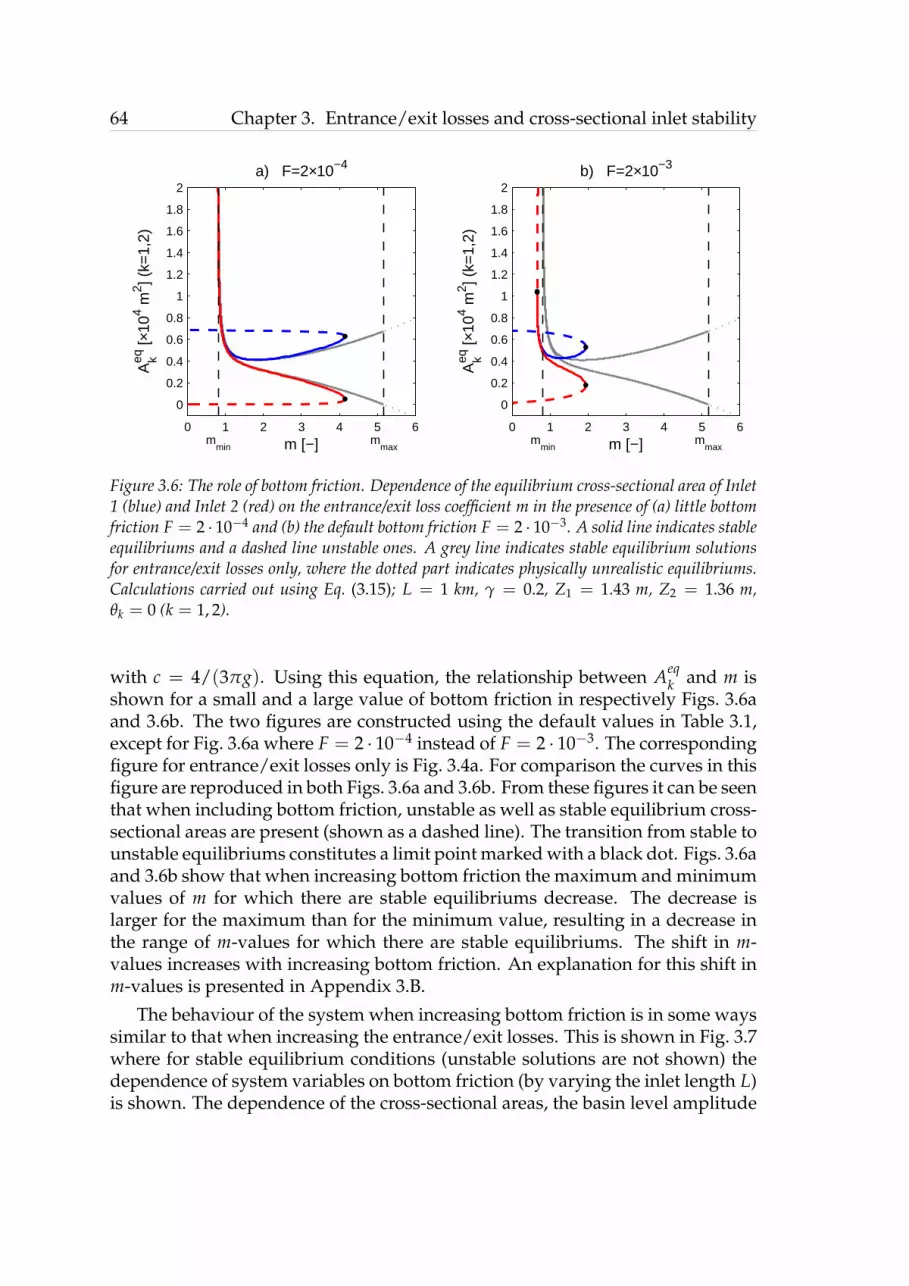
64 Chapter 3. Entrance/exit losses and cross-sectional inlet stability
0 1 2 3 4 5 6
0
0.2
0.4
0.6
0.8
1
1.2
1.4
1.6
1.8
2
mmax
mmin
a) F=2×10⁻⁴
m [−]
Akeq
[×10
4 m2 ] (
k=1,
2)
0 1 2 3 4 5 6
0
0.2
0.4
0.6
0.8
1
1.2
1.4
1.6
1.8
2
mmax
mmin
b) F=2×10⁻³
m [−]
Akeq
[×10
4 m2 ] (
k=1,
2)Figure 3.6: The role of bottom friction. Dependence of the equilibrium cross-sectional area of Inlet1 (blue) and Inlet 2 (red) on the entrance/exit loss coefficient m in the presence of (a) little bottomfriction F = 2 · 10−4 and (b) the default bottom friction F = 2 · 10−3. A solid line indicates stableequilibriums and a dashed line unstable ones. A grey line indicates stable equilibrium solutionsfor entrance/exit losses only, where the dotted part indicates physically unrealistic equilibriums.Calculations carried out using Eq. (3.15); L = 1 km, γ = 0.2, Z1 = 1.43 m, Z2 = 1.36 m,θk = 0 (k = 1, 2).
with c = 4/(3πg). Using this equation, the relationship between Aeqk and m is
shown for a small and a large value of bottom friction in respectively Figs. 3.6aand 3.6b. The two figures are constructed using the default values in Table 3.1,except for Fig. 3.6a where F = 2 · 10−4 instead of F = 2 · 10−3. The correspondingfigure for entrance/exit losses only is Fig. 3.4a. For comparison the curves in thisfigure are reproduced in both Figs. 3.6a and 3.6b. From these figures it can be seenthat when including bottom friction, unstable as well as stable equilibrium cross-sectional areas are present (shown as a dashed line). The transition from stable tounstable equilibriums constitutes a limit point marked with a black dot. Figs. 3.6aand 3.6b show that when increasing bottom friction the maximum and minimumvalues of m for which there are stable equilibriums decrease. The decrease islarger for the maximum than for the minimum value, resulting in a decrease inthe range of m-values for which there are stable equilibriums. The shift in m-values increases with increasing bottom friction. An explanation for this shift inm-values is presented in Appendix 3.B.
The behaviour of the system when increasing bottom friction is in some wayssimilar to that when increasing the entrance/exit losses. This is shown in Fig. 3.7where for stable equilibrium conditions (unstable solutions are not shown) thedependence of system variables on bottom friction (by varying the inlet length L)is shown. The dependence of the cross-sectional areas, the basin level amplitude

3.4. Bottom friction and inertia 65
0 0.5 1 1.5 2 2.50
1
2
3
4
5
6
7
8
a) Akeq vs. L
L [km]
Akeq
[×10
3 m2 ] (
k=1,
2)
0 0.5 1 1.5 2 2.51.36
1.37
1.38
1.39
1.40
1.41
1.42
1.43
b) Zbeq vs. L
L [km]Z
beq [m
]0 0.5 1 1.5 2 2.5
−30
0
30
60
90
120
150
180
c) φeq and ψkeq vs. L
L [km]
φeq a
nd ψ
keq [°
] (k=
1,2)
Figure 3.7: The role of bottom friction. Dependence of (a) stable equilibrium cross-sectional areasfor Inlet 1 (blue) and 2 (red), (b) the amplitude of the basin water level, and (c) the phases of thebasin water level (black) and the velocity in Inlet 1 (blue) and Inlet 2 (red) on bottom friction(L) for equilibrium conditions. Calculations carried out using Eq. (3.15); m = 1, F = 2 · 10−3,γ = 0.2, Z1 = 1.43 m, Z2 = 1.36 m, θk = 0 (k = 1, 2).
and the phases of the basin level and inlet velocities in Inlet 1 and 2 on the inletlength is shown in respectively Fig. 3.7a, 3.7b and 3.7c. When only consideringentrance/exit losses these dependencies are displayed in Fig. 3.4. In comparingFigs. 3.4 and 3.7 it should be realised that in Fig. 3.7 in addition to bottom friction,entrance/exit losses (corresponding to m = 1) are present. Therefore, only thepart of Fig. 3.4 beyond m = 1 should be compared to Fig. 3.7. From this compar-ison it follows that Aeq
k , Zeqb , ϕeq, ψ
eqk (k = 1, 2) show the same trend for increasing
m and increasing L. In particular, Zeqb increases and ϕeq decreases with increas-
ing values of L. From this it can be concluded that, similarly to entrance/exitlosses, when bottom friction is increased, the equilibrium velocity is attained byan increase in basin level and a decrease in basin level phase.
3.4.2 Inertia
When adding inertia to Eq. (3.15) the effect on the range of m-values for whichstable equilibriums exist is shown in Fig. 3.8, together with the case for entrance/exit losses and bottom friction only (depicted as a grey line). This figure is con-structed using the default parameter values of Table 3.1. The curves in Fig. 3.8 arequalitatively similar. For this particular case adding inertia decreases the range of(physically realistic) m-values for which stable equilibriums exist. Results of ad-ditional numerical experiments (see also Fig. 3.9a) show that the effect of addinginertia is somewhat sensitive to the other parameter values and can also increasethe range of m-values for which stable equilibriums exist. Therefore, care shouldbe taken in generalising the foregoing conclusion.

66 Chapter 3. Entrance/exit losses and cross-sectional inlet stability
0 1 2 3 4 5 6
0
0.2
0.4
0.6
0.8
1
1.2
1.4
1.6
1.8
2
mmax
mmin
m [−]
Akeq
[×10
4 m2 ] (
k=1,
2)
Figure 3.8: The role of inertia. Dependence of the equilibrium cross-sectional area of Inlet 1 (blue)and Inlet 2 (red) on the entrance/exit loss coefficient m in the presence of bottom friction andinertia. A solid line indicates stable equilibriums and a dashed line unstable ones. A grey lineindicates equilibrium solutions for entrance/exit losses and bottom friction only. Calculation arecarried out using Eq. (3.2); F = 2 · 10−3, L = 1 km, γ = 0.2, Z1 = 1.43 m, Z2 = 1.36 m,θk = 0 (k = 1, 2).
3.4.3 Relative Importance of the Entrance/Exit LossTerm and the Bottom Friction Term
In the preceding subsection it is shown that bottom friction in the presence of en-trance/exit losses can lead to stable double inlet systems. However, from Fig. 3.6it follows that increasing the amount of bottom friction leads to a significantlysmaller range of m-values where stable equilibriums can be found. This suggeststhat there is a limit to the amount of bottom friction that can be added, such thatstable equilibriums still exist. This is further investigated in this subsection.
Using the continuation method, the range of m-values where stable equilib-riums are found in Fig. 3.8 (notice that this range between two limit points issimilar for Aeq
1 and Aeq2 ) is calculated for values of L ranging between 0 and 1.6
km. This results in the blue curve plotted in Fig. 3.9a. Each point on the curvecorresponds to a value of m, L and Aeq
k (k = 1, 2). Stable equilibriums are foundfor combinations of m, L and Aeq
k inside this curve. It follows that stable equi-

3.4. Bottom friction and inertia 67
0 1 2 3 4 5 60
0.2
0.4
0.6
0.8
1
1.2
1.4
1.6a) L vs. m
stable region
unstable region
m [−]
L [k
m]
0 0.05 0.1 0.15 0.2 0.25 0.30
0.005
0.01
0.015
0.02
0.025
0.03
0.035
stable region
unstable region
b) e/e loss term vs. bf term
m/2g [s2 m−1]
FL/
gRk [s
2 m−
1 ] (k=
1,2)
Figure 3.9: Relative importance of entrance/exit loss term and bottom friction term. (a) Valuesof entrance/exit loss coefficient m and inlet length L for which there are stable equilibriums. (b)Values of the entrance/exit loss term and bottom friction term for Inlet 1 (blue) and Inlet 2 (red)for which there are stable equilibriums. For the significance of the asterisk see text. Calculationscarried out using Eq. (3.2); F = 2 · 10−3, γ = 0.2, Z1 = 1.43 m, Z2 = 1.36 m, θk = 0 (k = 1, 2).
libriums exist for values of L smaller than approximately 1 km. In some cases Lcan be as high as approximately 1.5 km. As an example, the range of (physicallyrealistic) m-values where stable equilibriums are found for L = 1 km in Fig. 3.9a,i.e. between approximately 0.6 and 1.4, corresponds to the range of m-valuesfound in Fig. 3.8. Note that for L = 1 km a second range of m-values wherestable equilibriums are found exists between approximately 2.7 and 3.1. For thisrange, however, the m-values are physically unrealistic and therefore this rangeis not shown in Fig. 3.8. Furthermore, it can be seen that for very small L, i.e.negligible bottom friction and inertia, the range of m-values for which there arestable equilibriums lies between approximately 0.8 and 5.2, which correspondswith the values for mmin and mmax that follow from Eqs. (3.13) and (3.14) and thedefault parameter values from Table 3.3.
For each of the points on the curve in Fig. 3.9a the value of the bottom friction
term FL/(gγ√
Aeqk ) is calculated and plotted versus the entrance/exit loss term
m/(2g) in Fig. 3.9b. Because each point on the curve in Fig. 3.9a has differentvalues for Aeq
1 and Aeq2 (see also Fig. 3.8), the bottom friction term has a different
value for each inlet. The blue curve corresponds to Inlet 1 and the red curve toInlet 2. Values of F and γ are those listed in Table 3.1. To emphasise that a singlepoint on the blue curve in Fig. 3.9a corresponds to a point on both the blue curve(Inlet 1) and the red curve (Inlet 2) in Fig. 3.9b, black asterisks are added in bothfigures for m = 1 and thus m/(2g) = 0.05 s2 m−1. It can be seen from Fig. 3.9bthat, starting at zero bottom friction, when increasing the value of the bottom fric-

68 Chapter 3. Entrance/exit losses and cross-sectional inlet stability
1.16 1.21 1.26 1.31 1.36 1.41 1.46 1.51 1.560
1
2
3
4
5
6
FA
unstable region
stable region stab
le re
gion
a) m vs. Z1
Z1 [m]
m [−
]
1.16 1.21 1.26 1.31 1.36 1.41 1.46 1.51 1.560
0.5
1
1.5
2
2.5
3
3.5
4
FA
unstable region
stable region stab
le re
gion
b) L vs. Z1
Z1 [m]
L [k
m]
Figure 3.10: Dependence of stable equilibriums on the ocean tidal amplitude of Inlet 1. (a) Valuesof Z1 and m for which stable equilibriums exist, where L = 1 km. (b) Values of Z1 and L for whichstable equilibriums exist, where m = 1. The green solid dot corresponds with parameter valuesfor the symmetric Faro-Armona system. The grey box indicates the assumed range of parametervalues for the asymmetric system (see text Section 3.6). Calculations carried out using Eq. (3.2);F = 2 · 10−3, γ = 0.2, Z2 = 1.36 m, θk = 0 (k = 1, 2).
tion term the range of m-values for which there are stable equilibriums generallydecreases. This is in agreement with the observations made in Subsection 3.4.1.For a given value of the entrance/exit loss term there is a limit to the bottomfriction that can be added. The limit value of the bottom friction term is in mostcases smaller than the corresponding value of the entrance/exit loss term. Takingas a typical value m = 1 and thus m/(2g) = 0.05 s2 m−1, corresponding to theblack asterisks in Fig. 3.9b, the maximum of the bottom friction term for Inlet 1is approximately 0.028 and for Inlet 2 approximately 0.015. This results in a ratioof entrance/exit loss term and bottom friction term of respectively 1.79 and 3.3.In conclusion the entrance/exit loss term has to be considerably larger than thebottom friction term for a double inlet system to be stable.
3.5 Effect of forcing on stable equilibriums
Parameters in the forcing are Zk and θk (k = 1, 2). In Section 3.3 it is shownthat for entrance/exit losses only, ocean tidal amplitudes and amplitude differ-ences determine whether or not stable equilibriums exist. The effect of the oceantidal amplitude when using the complete dynamic equation is demonstrated inFigs. 3.10a and 3.10b where the regions of stable equilibriums are plotted in re-

3.5. Effect of forcing on stable equilibriums 69
1.11 1.16 1.21 1.26 1.31 1.36 1.41 1.46 1.51 1.56 1.61−8
−7
−6
−5
−4
−3
−2
−1
0
1
2
3
4
5
6
7
8
FA
A
E
B
D
C
C
D
B
E
A
Z1 [m]
∆θ [d
eg]
A: L = 0.5 kmB: L = 1 kmC: L = 2 kmD: L = 3 kmE: L = 4 km
Figure 3.11: Regions in which stable equilibriums exist for different values of Z1, ∆θ = θ1 − θ2and L. The red region indicates the default case (Table 3.3) with L = 1 km. The solid greendot corresponds with parameter values for the symmetric Faro-Armona system. The grey boxindicates the assumed range of parameter values for the asymmetric system (see text Section 3.6).For explanation of the dashed vertical line see text Section 3.5. The red region indicates the regionfor the symmetric Faro-Armona case with L = 1 km. Calculations carried out using Eq. (3.2);m = 1, F = 2 · 10−3, γ = 0.2, Z2 = 1.36 m, θ2 = 0.
spectively the (Z1, m)-space and the (Z1, L)-space. The parameters m and L canbe interpreted as measures for respectively the entrance/exit losses and the bot-tom friction losses. It follows from Fig. 3.10a that for increasing Z1-values andkeeping Z2 constant at 1.36 m, the range of m-values for which there are stableequilibriums shifts to larger values of m. Similarly to m it follows from Fig. 3.10bthat for increasing Z1-values and keeping Z2 constant at 1.36 m, the range of L-values for which there are stable equilibriums shift to larger L-values.
The influence of phase differences between the ocean tides ∆θ = θ1 − θ2 onthe presence of stable equilibriums is demonstrated in Fig. 3.11. This figure isbased on a practical situation for which it is generally assumed that F = 2 · 10−3
and m = 1. In the figure ∆θ is plotted versus Z1 with L as parameter. The range ofZ1-values between the dashed lines (red region) correspond to the default case

70 Chapter 3. Entrance/exit losses and cross-sectional inlet stability
with L = 1 km and m = 1. This range corresponds with the range for Z1 inFig. 3.10a with m = 1 and in Fig. 3.10b with the range for Z1 for L = 1 km. FromFig. 3.11 the following general conclusions can be drawn.
• Z1 = Z2. No curve crosses the ordinate. This was further confirmed bycalculations with L < 0.5 km (not shown here). Therefore, phase differ-ences between the inlets alone cannot cause a double inlet system to be ina stable equilibrium. A similar conclusion was arrived at when discussingentrance/exit losses only; see Section 3.3.
• Z1 6= Z2. Phase differences between the ocean tides affect the stability re-gion, i.e. the range of Z1-values for which there are stable equilibriums. Asan example for L = 2 km, increasing ∆θ from 0 to 1 increases the range ofZ1-values for which there are stable equilibriums from 1.47 < Z1 < 1.49 to1.42 < Z1 < 1.48.
• θ1 = θ2 and θ1 6= θ2. For stable equilibriums the difference between Z1 andZ2 increases for increasing bottom friction (increasing L). As an examplefor Z1 > Z2, the values of Z1 are larger for L = 4 km than for L = 0.5 km.
3.6 The Faro-Armona double inlet system
The Faro-Armona double inlet system was already introduced in Section 1.3.Summarising, it is the western sub-system of the multiple-inlet barrier island sys-tem Rıa Formosa on the southern coast of Portugal (see Fig 1.3 on page 7). It con-sists of the Armona, Faro and Ancao Inlets, and covers approximately 3.4×10⁷
m2. The Faro and Armona Inlets capture 90% of the tidal prism of the westernsub-system and, moreover, there exists a relatively long winding connection be-tween Faro/Armona Inlets and Ancao Inlet (Salles et al., 2005, and referencestherein). This suggests that, as a first approximation, the Faro and Armona In-lets can be treated as a double inlet system only. Furthermore, the Faro-Armonasystem may be considered stable (Pacheco et al., 2011a).
For our approach to be applicable to the Faro-Armona system, typical val-ues of bulk parameters are estimated using observations and modelling resultspresented in Salles et al. (2005); Dias & Sousa (2009); Pacheco et al. (2010, 2011a,b)and references therein. Geometrical parameters were also estimated using GoogleEarth. Specifically, to determine the shape factor for the Faro and Armona Inlets,a rectangular cross-sectional area is assumed. From the above mentioned sourcescharacteristic ranges of parameters were found, see Column 2 and 4 of Table3.3. Based on these parameter ranges and making some reasonable assumptionsthe most likely parameter values for the system used for the lumped parametermodel are listed in the third and fifth column of Table 3.3. In Table 3.3 tidal am-plitudes pertain to spring tide conditions as observed off the inlets (Stations Fand H in Dias & Sousa (2009), Fig. 5).

3.6. The Faro-Armona double inlet system 71
Table 3.3: Parameter Values Representative for the Faro-Armona double inlet system
Armona Inlet (1) Faro Inlet (2)Parameter Range Model Range Model
InletsAi (m2) ∼ 2, 000 (c),(d) variable ∼ 4, 000 (c),(d) variableLi (km) 0.5− 1 (f) 0.7 1− 2 (d),(f) 2mi (-) 0.75− 1.25 (e) 1 0.75− 1.25 (e) 1γi (-) 0.05− 0.13 (a) 0.12 0.2− 0.37 (a),(d) 0.2Fi (-) 0.002− 0.0027 (a) 0.002 0.0011− 0.002 (a),(d) 0.002Ueq (m s−1) ∼ 1.05 (c) 1 0.9− 1.18 (a) 1Forcingω* (s−1) - 1.4× 10⁻⁴
Zi (m) ∼ 1.43 (b) 1.43 ∼ 1.36 (b) 1.36∆Z* (m) 0.01− 0.1 (b),(c) 0.07∆θ* (deg) -4− 0 (b) 0GeneralB (m2) ∼ 2.5× 10⁷ (c) 2.5× 10⁷ ∼ 0.9× 10⁷ (c) 0.9× 10⁷
M* (m3 year−1) 4× 10⁴ − 3× 10⁵(d),(e) 1×10⁵
a Salles et al. (2005) b Dias & Sousa (2009) c Pacheco et al. (2010) d Pacheco et al.(2011a) e Pacheco et al. (2011b) f Google Earth * pertaining to the entire system
Using the parameter values in Column 3 and 5 of Table 3.3 it is of interestto show how far the conditions for stability derived in Sections 3.3-3.5 are satis-fied keeping in mind that these conditions were derived for a symmetric system.When neglecting bottom friction and inertia in the dynamic equation and onlyincluding entrance/exit losses the range of m-values for a stable system is be-tween 0.8 and 5.2 (Eqs. (3.13) and (3.14)). When including bottom friction boththe maximum and minimum values are slightly reduced. Adding inertia the min-imum m-value slightly decreases and the maximum m-value slightly increases.It seems safe to conclude that the adopted value m = 1 satisfies the condition forstability. A second condition is that entrance/exit losses are considerably largerthan bottom friction losses. Using m = 1 for both inlets it follows that the en-trance/exit loss term m/(2g) ≈ 0.05 s2 m−1. Taking for Armona Inlet F1 = 0.002,L1 = 0.7 km, γ1 = 0.12, A1 = 2, 000 m2 and for Faro-Alhao Inlet F2 = 0.002,L2 = 2 km, γ2 = 0.2, A2 = 4, 000 m2, bottom friction terms FL/(gR) of approx-imately 0.026 and 0.032 s2 m−1, respectively, are obtained. Thus, for both inletsthe entrance/exit loss term is larger than the bottom friction term.
In the forgoing it is shown that a symmetric system resembling Faro-Armonasatisfies the theoretically derived conditions for cross-sectional stability. Refer-ring to Fig. 3.2, for this system a stable equilibrium is indeed present. To inves-tigate if this is also the case for the actual asymmetric system a flow diagramis constructed using the most likely parameter values for Faro-Armona listed

72 Chapter 3. Entrance/exit losses and cross-sectional inlet stability
0 2 4 6 80
2
4
6
8a) m=1
AArmona
[×103 m2]
AF
aro [×
103 m
2 ]
0 2 4 6 80
2
4
6
8b) m=0
AArmona
[×103 m2]A
Far
o [×10
3 m2 ]
Figure 3.12: Flow diagram for Faro-Armona double inlet system when (a) including entrance/exitlosses: m = 1 and (b) excluding entrance/exit losses: m = 0. The blue and red solid linecorrespond to the equilibrium flow curves of Armona and Faro, respectively, the grey vectorsindicate the direction in which the values of the cross-sectional areas change when they are notin equilibrium, the black circles indicate an unstable equilibrium and the black cross indicates astable equilibrium. Calculations carried out using Eq. (3.2); F = 0.002, L1 = 0.7 km, L2 = 2km, γ1 = 0.12, γ2 = 0.2, Z1 = 1.43 m, Z2 = 1.36 m, ∆θ = 0.
in Columns 3 and 5 of Table 3.3. The flow diagram is presented in Fig. 3.12aand, next to three unstable equilibriums, shows a stable equilibrium with cross-sectional areas of approximately 3,000 m2 for Armona and 4,000 m2 for Faro. Thisis close to the observed values listed in Table 3. In Fig. 3.12b the same flow dia-gram is presented for m = 0: no stable equilibriums are present, illustrating theimportance of including entrance/exit losses in the stability analysis.
In Figs. 3.10 and 3.11 in the previous section the grey boxes indicate the rangeof parameter values from Columns 2 and 4 of Table 3.3. Keeping in mind thatFigs. 3.10 and 3.11 pertain to a symmetric system discussed in Section 3.2.2, thegrey boxes show that depending on the choice of the value of the particular pa-rameter the system can be stable or unstable.
3.7 Discussion
The present approach to evaluate cross-sectional stability is based on the premisethat when at equilibrium the amplitude of the tidal velocity in both inlets isclose to 1 m s−1. Velocities in the inlets are calculated using a lumped-parametermodel. Using this approach it is shown that double inlets can be stable providedbottom friction and inertia in the inlet are small compared to entrance/exit losses.Essentially this limits cross-sectional stability to double inlet systems with rela-

3.7. Discussion 73
tively short inlets. In addition, the amplitudes of the tides off the two inlets haveto be different.
Referring to Figs. 3.10 and 3.11, cross-sectional stability is limited to a rela-tively narrow range of parameter values. Parameters include the entrance/exitloss coefficient m, the bottom friction factor F, the basin surface area B and theinlet length L. In addition, there is the value of the equilibrium velocity Ueq. Inparticular, the values of m and F require calibration and validation of the lumped-parameter model. In applying the stability analysis to the Faro-Armona systemvalues of m and F were ascertained from previous studies carried out by otherinvestigators. Inlet length was also estimated from Google Earth. Values of theamplitudes of the offshore tide were determined from measurements. The valueof Ueq was taken from the literature and taken as a constant value to allow ananalytical approach. Even though the 1 m s−1 for the equilibrium velocity is agenerally accepted value, starting with the empirical cross-sectional area tidalprism relationship (A-P relationship), recent studies suggest that this value is a(weak) function of littoral drift and cross-sectional area rather than a constant(van de Kreeke, 2004).
The fact remains that the zero-dimensional lumped-parameter model includ-ing the assumption of a pumping mode for the basin represents a simplificationof an essentially 2D hydrodynamics problem. Admittedly, this is a simplificationthat, similar to the constant value of Ueq, was introduced to allow an analyticalapproach to derive conditions for stability. The ability of the lumped-parametermodels to capture the dynamics of the flow was shown in Herman (2007) whoapplied both a 2D hydrodynamics model and a lumped-parameter model to in-lets in the German Wadden Sea.
In view of the sensitivity of the stability to the various parameters in thelumped-parameter model as well as the assumed stability criterion (the equi-librium velocity), the present application to the Faro-Armona system is of a di-agnostic nature. To arrive at a predictive approach it is suggested to combineresults obtained with the type of models used in this paper and process-basedmodels in which water motion and sediment transport are based on physicalfirst principles (e.g, de Vriend & Ribberink, 1996; Pacheco et al., 2011b; Nahonet al., 2012; Tung et al., 2012; Wang & Beck, 2012). At present, neither of thesemodels can be used to make predictions. Therefore, it is important to improveboth the lumped-parameter models and process-based morphodynamic modelsfor tidal inlets. A possible first step to improve the lumped-parameter model is toinvestigate the applicability and limitations of the pumping mode assumption.With regards to the Faro-Armona system an improved estimate of the equilib-rium velocity could be obtained if for this part of the Portuguese coast the APrelationship was known.

74 Chapter 3. Entrance/exit losses and cross-sectional inlet stability
3.8 Conclusions
In evaluating the cross-sectional stability of tidal inlets it has been customaryto describe the hydrodynamics with a lumped-parameter model. In this modelthe dynamics of the flow in the inlet constitutes a balance between inertia, en-trance/exit losses and bottom friction on the one hand and the pressure gradientacross the inlet on the other hand. A pumping mode is assumed for the basin.
In this chapter the role of inertia, entrance/exit losses and bottom friction onthe cross-sectional stability of a double inlet system is investigated with emphasison entrance/exit losses. The reason for this is that results of previous studies sug-gest that when neglecting entrance/exit losses no stable equilibriums are present.In the present study both analytical models and numerical experiments are used.To allow a physical explanation of the various terms in the lumped-parametermodel use is made of a simplified version of the Faro-Armona system in whichthe length, friction factor and entrance/exit loss coefficient are the same for bothinlets and the offshore tides may differ. The Faro-Armona double inlet system ispart of the Rıa Formosa, Portugal. This inlet system can be considered to be instable equilibrium.
The model results in this chapter lead to the following conclusions. Whenretaining only entrance/exit losses and neglecting inertia and bottom friction,stable equilibriums are possible provided the two off-shore water level ampli-tudes are different. A difference in phase between the ocean tides does not leadto stable inlets.
Adding bottom friction, stable equilibriums exist provided the entrance/exitloss term is considerably larger than the bottom friction term. Increasing bottomfriction leads to a downward shift and narrowing of the range of entrance/exitloss coefficients for which stable equilibriums exist.
Adding inertia, thus using the complete dynamic equation, somewhat affectsthe range of values of the entrance/exit loss coefficient for which stable cross-sections exist. Depending on the various parameter values the range can eitherincrease or decrease.
In addition to the terms in the dynamic equation, the magnitude of the am-plitudes of the off-shore tides and their differences affect the presence of stableequilibriums. For example, for stable equilibriums to exist an increase in thedifference between the amplitude requires an increase in the entrance/exit lossterm and/or an increase in the bottom friction term. Phase differences betweenthe off-shore tides affect the range of amplitude differences where stable equilib-riums exist.
For the simplified symmetric version of the Faro-Armona system it is shownthat the presence of stable equilibriums is sensitive to the selection of parametervalues such as inlet length, bottom friction factor and entrance/exit loss coef-ficient. This makes it difficult for practical cases to use the lumped-parametermodel as a predictive tool.

3.8. Conclusions 75
Applying the stability analysis to the actual Faro-Armona system and judi-ciously selecting parameter values it is shown that the stability of this systemcan be explained (as opposed to predicted) using the lumped-parameter modeltogether with the condition that inlets are stable when the velocity amplitudeequals the equilibrium velocity (∼ 1 m s−1).

76 Chapter 3. Entrance/exit losses and cross-sectional inlet stability
3.A Entrance/Exit Losses Only
In this appendix the analytical derivations to support the explanation of the roleof the entrance/exit loss coefficient m on the equilibrium and stability of doubleinlet systems are given.
3.A.1 Basin Tide and Inlet Velocities
Neglecting inertia and bottom friction, the linearised equations for the water mo-tion in the inlets are:
cmUequk = ζk − ζb, k = 1, 2, (3.A.1)
with, c = 4/(3πg). Assuming a pumping mode for the basin the continuityequation is:
Bdζbdt
= A1u1 + A2u2. (3.A.2)
The open boundary condition, which now only allows amplitude differences, is:
ζk = <
Zkeiωt
, (3.A.3)
where < is the real part and Zk is real-valued. To arrive at an analytical solutionfor the basin tide and inlet velocities the following trial solutions are introduced:
ζb ∼ <
Zbei(ωt+ϕ)
, (3.A.4)
uk ∼ <
Ukei(ωt+ψk)
, (3.A.5)
where Zb and Uk are real-valued. Eliminating uk between Eqs. (3.A.1) and (3.A.2)results in an equation for the basin tide ζb. Substituting ζk and the trial solu-tion for ζb in this equation and separating into real and imaginary parts leads toexpressions for the amplitude Zb and phase ϕ of the basin tide. It follows that
tan ϕ =−µmUeq
(A1 + A2), (3.A.6)
where µ = cωB. The phase ϕ is in the fourth quadrant, i.e. −π/2 < ϕ < 0.As expected, the sea surface elevation precedes the basin surface elevation. Theamplitude of the basin tide is
Zb =(A1Z1 + A2Z2)√
(µmUeq)2 + (A1 + A2)2. (3.A.7)

3.A. Entrance/Exit Losses Only 77
Substituting the trial solution for uk in Eq. (3.A.1) and separating into real andimaginary parts leads to expressions for the amplitude Uk and phase ψk of the in-let velocity as a function of the known expressions Zb (Eq. 3.A.7) and ϕ (Eq. 3.A.6).Substituting these expressions it follows that
tan ψk =µmUeq(A1Z1 + A2Z2)
((µmUeq)2 + (A1 + A2)2)Zk − (A1Z1 + A2Z2)(A1 + A2). (3.A.8)
When deriving the expression for sin ψk from Eq. (3.A.8), it follows that it isalways positive and thus ψk is located in the first or second quadrant. FromEq. (3.A.8) it then follows that ψk is in the first quadrant when the denominatoris positive and in the second quadrant when the denominator is negative. In bothcases the velocity precedes the ocean tide. The amplitude of the inlet velocity is
Uk =1
cmUeq
√(µmUeqZk)2 + A2
3−k(Z1 − Z2)2
(µmUeq)2 + (A1 + A2)2 . (3.A.9)
3.A.2 Conditions for Equilibrium Cross-Sections forZ1 6= Z2
Eliminating ζb between Eqs. (3.A.1) and (3.A.2) results in two equations in u1and u2. Substituting the trial solutions for uk (Eq. 3.A.5) and taking Uk = Ueq,two equations are obtained with the equilibrium cross-sectional areas Aeq
1 andAeq
2 as unknowns:
(Aeq1 + iµmUeq)Ueqeiψeq
1 + Aeq2 Ueqeiψeq
2 = iωBZ1, (3.A.10)
(Aeq2 + iµmUeq)Ueqeiψeq
2 + Aeq1 Ueqeiψeq
1 = iωBZ2. (3.A.11)
Writing the real and imaginary parts of Eqs. (3.A.10) and (3.A.11) it can be shownthat for Z1 6= Z2 these equations can only be satisfied provided the phases of theinlet velocities are related as ψ
eq2 = π − ψ
eq1 . Making use of this, the following
solution for Aeqk is obtained:
Aeqk =
µmsin ψ
eq1
[Z1 + Z2
4cmUeq− (−1)kUeq
(1− cos2 ψ
eq1
2 cos ψeq1
)]. (3.A.12)
Subtracting the imaginary parts of Eqs. (3.A.10) and (3.A.11) and substituting ψeq2
it follows that
cos ψeq1 =
∆Z2cmU2
eq, (3.A.13)
78 Chapter 3. Entrance/exit losses and cross-sectional inlet stability
where ∆Z = Z1− Z2. As shown in Appendix 3.A.1, depending on the sign of thedenominator of Eq. (3.A.8), ψ
eq1 is in the first or second quadrant. It follows from
Eq. (3.A.13) that for inlets that are in equilibrium and ∆Z > 0, ψeq1 is in the first
quadrant.With sin ψ
eqk positive (see Appendix 3.A.1) a requirement for Aeq
k to be positiveis that the expression between square brackets in Eq. (3.A.12) is positive. With theexpression for cos ψ
eq1 given by Eq. (3.A.13) this leads to the condition
Z1∆Z2(cm)2U4
eq≥ 1, ∆Z > 0. (3.A.14)
A second condition for Eq. (3.A.12) to be a valid solution for Aeqk is that the abso-
lute value of cos ψeq1 is equal to or smaller than one, and thus from Eq. (3.A.13)
∆Z2cmU2
eq≤ 1, ∆Z > 0. (3.A.15)
Similar conditions as expressed by Eqs. (3.A.14) and (3.A.15) hold for ∆Z < 0. Inthat case in Eq. (3.A.14) Z1 is replaced by Z2 and in Eqs. (3.A.14) and (3.A.15) ∆Zis replaced by −∆Z.
3.A.3 The Role of the Entrance/Exit Loss Coefficientm
From Eqs. (3.A.14) and (3.A.15) it follows that for given Z1 and Z2 there is onlya limited range of m-values for which equilibrium cross-sectional areas exist; seeexpressions for mmin, Eq. (3.13), and mmax, Eq. (3.14). In the following the effectof varying m on Aeq
k , ζeqb , ϕeq and ψ
eqk is investigated, where it is assumed that
Z1 > Z2. To show the effect on Aeqk , values of Aeq
k are evaluated for m = mminand m = mmax. As explained in Appendix 3.A.2, m = mmin corresponds to| cos ψ
eq1 | = 1 and thus sin ψ
eq1 = 0. It then follows from Eq. (3.A.12) that Aeq
kgoes to infinity. For m = mmax and k = 2 the term between square brackets inEq. (3.A.12) is zero and thus Aeq
2 = 0. The value of Aeq1 is positive and finite.
Furthermore, it follows from Eq. (3.A.12) that, with cos ψ1 positive, Aeq1 > Aeq
2 .To evaluate the effect of varying m on ζ
eqb , ϕeq and ψ
eqk the trial solutions,
Eqs. (3.A.4) and (3.A.5), and open boundary condition, Eq. (3.A.3), are substi-tuted in Eq. (3.A.1). The real and imaginary parts of the resulting equation are
< : cmUeqUk cos ψk = Zk − Zb cos ϕ, (3.A.16a)= : cmUeqUk sin ψk = −Zb sin ϕ. (3.A.16b)

3.A. Entrance/Exit Losses Only 79
Squaring and adding Eqs. (3.A.16a) and (3.A.16b) and substituting Uk = Ueqresults in
(cm)2U4eq =
(Zk − Zeq
b cos ϕeq)2+ (Zeq
b )2 sin2 ϕeq. (3.A.17)
Subtracting the equations for k = 1 and k = 2 yields
Z1 − Zeqb cos ϕeq = ±(Z2 − Zeq
b cos ϕeq). (3.A.18)
Because of the assumption Z1 > Z2 the positive variant of Eq. (3.A.18) is notpossible. Therefore, from (3.A.18) it follows that
Zeqb cos ϕeq =
Z1 + Z2
2. (3.A.19)
Substituting for Zeqb cos ϕeq in Eq. (3.A.17) yields
(cm)2U4eq =
(∆Z2
)2
+ (Zeqb )2 sin2 ϕeq. (3.A.20)
With the expression for mmin (Eq. 3.13), it follows from Eq. (3.A.20) that sin ϕeq =0 and, thus, with ϕeq in the fourth quadrant ϕeq = 0. It then follows fromEq. (3.A.19) that
Zeqb =
Z1 + Z2
2. (3.A.21)
With m = mmin, the water level in the basin lies between the two ocean waterlevels. Using Eqs. (3.A.13) and (3.13), the phase angles of the velocity are ψ
eq1 = 0
and ψeq2 = π. Summarizing, for m = mmin, Zeq
b is given by Eq. (3.A.21), ϕeq = 0,Uk = Ueq, ψ
eq1 = 0 and ψ
eq2 = π.
Eliminating ϕeq between Eqs. (3.A.19) and (3.A.20) results in
(Zeqb )2 = (cm)2U4
eq + Z1Z2, (3.A.22)
and thus Zeqb increases with increasing values of m. It then follows from Eq. (3.A.19)
that cos ϕeq decreases. With ϕeq in the fourth quadrant this implies decreasingvalues of ϕeq for increasing values of m. The basin tide increasingly lags theocean tide. From (3.A.13) and with ψ
eq1 in the first quadrant it follows that for
increasing values of m, ψeq1 increases and, with ψ
eq2 = π − ψ
eq1 , ψ
eq2 decreases.
Summarizing, for increasing values of m, Zeqb and ψ
eq1 increase and ϕeq and ψ
eq2
decrease.

80 Chapter 3. Entrance/exit losses and cross-sectional inlet stability
3.B Entrance/Exit Losses and Bottom Fric-tion
This appendix explains the change in the range of m-values for which there arestable equilibriums when in addition to entrance/exit losses bottom friction isincluded in the dynamic equations. The shift in the lower limit of m can be ex-plained realizing that in the neighbourhood of m = mmin the equilibrium cross-sectional areas Aeq
1 and Aeq2 are large and thus bottom friction is small. From this
it is concluded that in the neighbourhood of m = mmin bottom friction has littleeffect on the basin level and thus on the water level difference between oceanand basin when the system is in equilibrium. Writing Eq. (3.15) for equilibriumconditions results in
c
m +2FL
γ√
Aeqk
U2eq = (ζk − ζb)
eq. (3.B.1)
With the right-hand side being the same with and without bottom friction it thenfollows that for a given equilibrium state adding bottom friction requires that theentrance/exit losses decrease and thus the value of m decreases.
In explaining the downward shift of the maximum m-value the amount ofbottom friction that is added is assumed to be small compared to the entrance/exitlosses. In that case it is reasonable to assume that in the neighbourhood ofm = mmax the qualitative behaviour of Zeq
b , Aeq1 and Aeq
2 as a function of m isthe same as in the absence of bottom friction, i.e. Zeq
b increases and Aeq2 decreases
with increasing values of m and Aeq1 Aeq
2 .When including bottom friction the governing equations for inlet 1 and 2 are
respectively
cUeq
(m + 2FL
γ√
A1
)u1 = ζ1 − ζb, (3.B.2)
cUeq
(m + 2FL
γ√
A2
)u2 = ζ2 − ζb. (3.B.3)
Substituting the trial solutions for ζb and uk, respectively Eqs. (3.A.4) and (3.A.5),separating into real and imaginary parts and, subsequently, squaring and addingthese parts results in
(cUeq)2(
m +2FL
γ√
A1
)2
U21 = Z2
1 + Z2b − 2Z1Zb cos ϕ, (3.B.4)
(cUeq)2(
m +2FL
γ√
A2
)2
U22 = Z2
2 + Z2b − 2Z2Zb cos ϕ. (3.B.5)

3.B. Entrance/Exit Losses and Bottom Friction 81
Writing Eqs. (3.B.4) and (3.B.5) for equilibrium conditions yields
c2U4eq
m +2FL
γ√
Aeq1
2
= Z21 + (Zeq
b )2 − 2Z1Zeqb cos ϕeq, (3.B.6)
c2U4eq
m +2FL
γ√
Aeq2
2
= Z22 + (Zeq
b )2 − 2Z2Zeqb cos ϕeq. (3.B.7)
Eliminating Zeqb cos ϕeq between Eqs. (3.B.6) and (3.B.7) the following expression
for Zeqb as a function of m, Aeq
1 and Aeq2 is derived
(Zeqb )2 =(cm)2U4
eq + Z1Z2 + c2U4eq
(Z2
Z2 − Z1
) 4mFL
γ√
Aeq1
+
2FL
γ√
Aeq1
2
− c2U4eq
(Z1
Z2 − Z1
) 4mFL
γ√
Aeq2
+
2FL
γ√
Aeq2
2 .
(3.B.8)
Making use of Aeq1 Aeq
2 , Eq. (3.B.8) is simplified to
(Zeqb )2 =(cm)2U4
eq + Z1Z2−
c2U4eq
(Z1
Z2 − Z1
) 4mFL
γ√
Aeq2
+
2FL
γ√
Aeq2
2 .
(3.B.9)
This equation relates m, Zeqb and Aeq
2 in the neighbourhood of m = mmax when thesystem is in equilibrium. The system is perturbed by increasing the value of m byan amount of ∆m (with ∆m positive) and keeping all other parameters constant.As a result the system is assumed to go to a new equilibrium. The resultingchanges in Zeq
b and Aeq2 are respectively ∆Zb and ∆A2. Here, it is assumed that
the perturbations are small compared to the equilibrium values. In Eq. (3.B.9)replacing m by meq + ∆m, Aeq
2 by Aeq2 + ∆A2 and Zeq
b by Zeqb + ∆Zb results in an
equation relating meq, Zeqb and Aeq
2 for a new equilibrium. This equation can be
further simplified by expanding 1/√
Aeq2 in a Taylor series and only considering
terms of perturbed order, i.e. ∆m, ∆Zb and ∆A2. The result is

82 Chapter 3. Entrance/exit losses and cross-sectional inlet stability
∆m · 2c2U4eq
meq(
Z1 − Z2
Z1
)+
2FL
γ√
Aeq2
=
∆Zb · 2Zeqb
[Z1 − Z2
Z1
]+
∆A2 · 2c2U4eq
meqFLγ(Aeq
2 )3/2+ 2
(FL
γAeq2
)2 .
(3.B.10)
In this equation, the expressions in square brackets are all positive (Z1 > Z2). Be-cause Zeq
b increases and Aeq2 decreases with increasing values of m, ∆Zb is positive
and ∆A2 is negative. It then follows from Eq. (3.B.10) that for ∆m to be positivethe term multiplying ∆Zb has to be larger than the absolute value of the termmultiplying ∆A2, which is only possible for Aeq
2 > 0. In turn, this implies that inthe presence of bottom friction the maximum value of m for which equilibriumis possible is smaller than mmax.
3.C. Linear Stability Entrance/Exit Losses Only 83
3.C Linear Stability Entrance/Exit Losses Only
In this appendix the linear stability of the equilibrium for entrance/exit lossesonly, as summarised in Section 3.3, is discussed in detail. Linear stability is in-vestigated by considering Eq. (3.1), which determines the rate of change of theequilibrium after a perturbation:
Ak = Aeqk + ∆Ak. (3.C.1)
Here, it is assumed that the equilibrium value is much larger than the perturba-tion, i.e. Aeq
k ∆Ak. Next, the system of Eq. (3.1) for k = 1, 2 is linearised aroundthe equilibrium solution (i.e. only terms linear in the perturbation are retained).Therefore, the amplitude of the inlet velocity Uk , Eq. (3.7), is linearised. The firstorder Taylor expansion for Uk around the equilibrium solution has the form
Uk(A1, A2) = Ueqk + ∆Uk
= Uk(Aeq1 , Aeq
2 ) + ∆A1∂Uk∂A1
∣∣∣(A1,A2)
+ ∆A2∂Uk∂A2
∣∣∣(A1,A2)
,(3.C.2)
where
∂Uk∂A1
∣∣∣∣(A1,A2)
=− 1cmUeq
√(µmUeqZk)2 + (A2)2(Z1 − Z2)2
(µmUeq)2 + (A1 + A2)2 ·(A1 + A2
(µmUeq)2 + (A1 + A2)2
),
(3.C.3)
and
∂Uk∂A2
∣∣∣∣(A1,A2)
=1
cmUeq
(1√
(µmUeqZk)2+A22(Z1−Z2)2
(µmUeq)2+(A1+A2)2
·
[A2(Z1 − Z2)
2
(µmUeq)2 + (A1 + A2)2
]−√
(µmUeqZk)2 + A22(Z1 − Z2)2
(µmUeq)2 + (A1 + A2)2 ·[A1 + A2
(µmUeq)2 + (A1 + A2)2
]).
(3.C.4)

84 Chapter 3. Entrance/exit losses and cross-sectional inlet stability
Here, c = 4/(3πg) and µ = cωB. Using Eq. (3.C.1) and considering only termsof perturbed order ∆Ak, it follows that:
∆Uk =1
(cm)2U3eq
(Aeq
3−k(Z1 − Z2)2
(µmUeq)2 + (Aeq1 + Aeq
2 )2
)∆A3−k−
Ueq
(Aeq
1 + Aeq2
(µmUeq)2 + (Aeq1 + Aeq
2 )2
)(∆A1 + ∆A2).
(3.C.5)
With Uk = Ueqk + ∆Uk the expression for dAk(Uk)/dt (Eq. 3.1) can be written as
dAkdt
(Uk) =ML
(1 + 3
∆UkUeq
+O(∆U2k )
)(3.C.6)
Considering only terms of perturbed order ∆Uk and substituting Eq. (3.C.5) inEq. (3.C.6) results in:
dAkdt
∣∣∣∣∆Ak
=3M
(cm)2U4eqL
( Aeq3−k(Z1 − Z2)
2∆A3−k
(µmUeq)2 + (Aeq1 + Aeq
2 )2−
(cm)2U4eq(Aeq
1 + Aeq2 )(∆A1 + ∆A2)
(µmUeq)2 + (Aeq1 + Aeq
2 )2
).
(3.C.7)
With ∆Ak = Akeλt the eigenvalue problem for Ak can now be written as
λ
[A1A2
]=
[−κξ κ (σ1 − ξ)
κ (σ2 − ξ) −κξ
] [∆A1∆A2
], (3.C.8)
with
κ =3M
(cm)2U4eqL
(1
(µmUeq)2 + (Aeq1 + Aeq
2 )2
),
ξ = (cm)2U4eq(Aeq
1 + Aeq2 ),
σk = Aeqk (Z1 − Z2)
2.
If <λ > 0, the equilibrium is unstable as the amplitude of the perturbationincreases in time. <λ < 0 indicates that the equilibrium is stable. The stabilityof the equilibrium can be deduced from the matrix in (3.C.8) by investigating itstrace and the determinant (i.e. without explicitly calculating the eigenvalues),as the trace is equal to the sum of the eigenvalues and the determinant to their
3.C. Linear Stability Entrance/Exit Losses Only 85
product. Hence, the conditions for a stable equilibrium are a negative trace anda positive determinant. From the matrix in (3.C.8) it follows that the trace isalways negative, since ζ and ξ are always positive. In the case of similar forcingamplitudes (σ1 = σ2 = 0), the determinant is zero. Hence, one eigenvalue iszero and the other negative. It can thus be concluded that for similar forcingamplitudes there are an infinite number of equilibriums on a straight line whichare neutrally stable. If the system is perturbed, it returns to equilibrium, but notnecessarily the same equilibrium.
For different forcing amplitudes (σ1 6= σ2) the determinant of the matrix in(3.C.8) is positive provided
Aeq1
Aeq2+
Aeq2
Aeq1
>(Z1 − Z2)
2
(cm)2U4eq− 2. (3.C.9)
It can be shown that the left-hand side of (3.C.9) is minimal, and equal to 2, ifboth equilibrium cross-sections are equal. Hence, if Z1 − Z2 < 2cmU2
eq, the de-terminant is always positive. From (3.11) it follows that if an equilibrium exists,Z1− Z2 is always smaller than 2cmU2
eq and, therefore, the determinant of the ma-trix in (3.C.8) is always positive. As the trace is negative and the determinantpositive, the equilibriums given by (3.C.9) are always stable. Summarizing, fordifferent forcing amplitudes and provided that an equilibrium exists, this equi-librium is always stable.


4Double inlet stability by
spatially varying watermotion*
Abstract The cross-sectional stability of double inlet system is investigatedusing an exploratory model that combines Escoffier’s stability concept for theevolution of the inlet’s cross-sectional area with a two-dimensional, depth-averaged(2DH) hydrodynamic model for tidal flow. The model geometry consists of fourrectangular compartments, each with a uniform depth, associated with the ocean,two tidal inlets and the basin. The water motion, forced by an incoming Kelvinwave at the ocean’s open boundary and satisfying the linear shallow water equa-tions on the f -plane with linearised bottom friction, is in each compartment writ-ten as a superposition of eigenmodes, i.e. Kelvin and Poincare waves. A collo-cation method is employed to satisfy boundary and matching conditions. Theanalysis of resulting equilibrium configurations is done using flow diagrams.
Model results show that internally generated spatial variations in the watermotion are essential for the existence of stable equilibriums with two inlets open.In the hydrodynamic model used in this chapter, both radiation damping into theocean and basin bottom friction result in these necessary spatial variations. Cori-
*This chapter is based on a paper (”Influence of basin geometry on equilibrium and stability of dou-ble inlet systems” by R.L. Brouwer, H.M. Schuttelaars and P.C. Roos (2012), In: Jubilee ConferenceProceedings NCK-days 2012: Crossing borders in coastal research, Enschede, The Netherlands,pp. 85-89.) and on a conference contribution (”Influence of basin characteristics on equilibrium andstability of double inlet systems” by R.L. Brouwer, H.M. Schuttelaars, P.C. Roos and J. van de Kreeke(2012), In: Book of abstracts of Physics of Estuaries and Coastal Seas 2012, New York, USA.). Ithas been submitted to appear in the Topical Collection - PECS 2012 of Ocean Dynamics.
87

88 Chapter 4. Double inlet stability by spatially varying water motion
olis effects trigger an asymmetry in the stable equilibrium cross-sectional areas ofthe inlets. Furthermore, more elongated basin geometries in the inlet-parallel di-rection generally correspond to significantly larger equilibrium values of the inletcross-sections. These model outcomes result from a competition between a desta-bilising (caused by inlet bottom friction) and a stabilising mechanism (caused byspatially varying local pressure gradients over the inlets).
4.1 Introduction
About ten percent of the world’s coastline consists of barrier coasts (Glaeser,1978). They generally display a chain of barrier islands separated by tidal in-lets that connect one or more back-barrier basins to an ocean or a coastal sea. Thecombination of tidal inlet and back-barrier basin is commonly known as a tidalinlet system. Examples are found along the Wadden Sea coast of the Netherlands,Germany and Denmark (see Fig. 1.2), the Rıa Formosa in southern Portugal (seeFig. 1.3) and the U.S. east coast. These morphologically dynamic systems aresubject to potentially conflicting interests of economy, coastal safety and ecology.
To manage these different interests, it is important to understand the long-term morphological evolution of these inlet systems and their adaptation to nat-ural changes (e.g., sea level rise, storm-induced barrier island breaching) andhuman interventions (e.g., basin reduction, dredging activities, inlet relocation).For example, the closure of the Zuiderzee (now called Lake IJssel) in the north-west of the Netherlands in 1932 induced extensive morphological changes in theDutch Wadden Sea that are still felt today (for more details see, e.g., Elias et al.,2003). An example of barrier island breaching occurred recently along the southshore of Long Island (NY) where Hurricane Sandy created three breaches on FireIsland, which led to (expensive) measures to close them again (National ParkService, 2012).
The stability properties of these systems can be inferred from the morpho-logical evolution of the cross-sectional area of the tidal inlets. For single inletsystems in equilibrium, various empirical relationships exist between the in-let’s cross-sectional area A and ebb-tidal prism P (e.g. LeConte, 1905; O’Brien,1931; Jarrett, 1976). Alternatively, Escoffier (1940) related the equilibrium cross-sectional area to a balance between the wave-driven import of sediment and thetide-driven sediment export, resulting in the definition of an equilibrium velocityUeq. If the ebb-tidal inlet velocity amplitude U is larger than the equilibrium ve-locity, U > Ueq, the inlet’s cross-sectional area increases (erodes), and if U < Ueqit decreases (accretes). An equilibrium is considered stable, when after beingperturbed, the cross-sectional area returns to its original equilibrium value. Tocalculate the amplitude of the inlet velocity, Escoffier used a simple hydrody-namic model (Brown, 1928) that assumes a uniformly fluctuating surface eleva-tion in the basin, and prescribed a sinusoidal forcing at the seaside. In general,

4.1. Introduction 89
one stable and one unstable equilibrium cross-sectional area exist (see Fig. 1.4 onpage 10).
van de Kreeke (1990a) extended Escoffier’s stability concept to double inletsystems, taking the Pass Cavallo-Matagorda Inlet system on the US Gulf coast asan example. For these systems, an equilibrium is considered stable, when afterbeing perturbed, the cross-sectional areas of both inlets return to their originalequilibrium values. Similarly to Escoffier (1940), in his model schematisation thesurface elevation in the basin was also assumed to fluctuate uniformly. Consid-ering a balance between bottom friction in the inlets and the pressure gradientover the inlet, he concluded that only unstable equilibriums exist, i.e. one inletcloses and the other remains open. This model result contradicts observationsin, for instance, the Dutch Wadden Sea (Louters & Gerritsen, 1994) and the Por-tuguese Rıa Formosa (Salles et al., 2005) where tidal inlet systems with more thanone inlet connecting the back-barrier basin to the ocean are stable on a historicaltime scale (∼centuries). This inconsistency between model results and observa-tions is probably due to the too-restrictive assumption of a uniformly fluctuatingbasin surface elevation: Escoffier (1977) already suggested that spatial variationsin basin surface elevation may lead to stable configurations with more than oneinlet open. In Chapters 2 (see also de Swart & Volp, 2012) and 3 it was shown thataccounting for these spatial variations explicitly, by implementing a topographichigh in the basin schematisation, or parametrically, by including entrance/exitlosses in the dynamic equation, stable equilibrium configurations with more thanone inlet open could be found. However, in these chapters the (sub-)basin surfaceelevation was still assumed to fluctuate uniformly, neglecting effects of basin bot-tom friction and geometry. In addition, the forcing off the inlets was prescribed,thereby neglecting the influence of the inlet system on the hydrodynamics onthe seaward side of the tidal inlets: this interaction will influence the surfaceelevations off the inlets by waves radiating away from the inlet into the ocean(radiation damping). Finally, Coriolis effects have been omitted so far, which arealso likely to influence the surface elevations in ocean, inlets and basin.
To scrutinise Escoffier’s (1977) suggestion, this chapter aims to investigate theinfluence of a spatially varying water motion on the cross-sectional stability ofdouble inlet systems. In particular, the individual contributions of basin bot-tom friction, radiation damping and Coriolis effects are examined. Therefore, Es-coffier’s concept of inlet stability is combined with a 2DH hydrodynamic model(see Taylor, 1920; Godin, 1965; Roos & Schuttelaars, 2011; Roos et al., 2011) basedon the linear shallow water equations in an idealised, rotating geometry consist-ing of ocean, tidal inlets and basin.
This chapter is organised as follows. In the following section the new 2DHmodel and solution method will be presented. Subsequently, in Section 4.3 thewater motion for a rotating double inlet system is discussed, as well as the in-fluence of radiation damping, basin bottom friction and Coriolis effects on thecross-sectional stability of double inlet systems. In addition, the effect of different

90 Chapter 4. Double inlet stability by spatially varying water motion
basin geometries is examined. Finally, Sections 4.4 and 4.5 contain the discussionand conclusions, respectively.
4.2 Model and method
4.2.1 Cross-sectional stability
In this study the focus is on cross-sectional stability of double inlet systems. Fol-lowing Escoffier (1940) an inlet is assumed to be in equilibrium if the amplitudeof the cross-sectionally averaged inlet velocity Up is equal to the so-called equi-librium velocity Ueq, generally taken as 1 m s−1 (Bruun et al., 1978). This equilib-rium velocity is defined as the amplitude of the tidal current that is just sufficientto flush the sediment carried into the inlet by the wave-induced alongshore cur-rent. Hence, inlets are in equilibrium (assuming average weather conditions asopposed to storm conditions) if there is a balance between the volume of sedi-ment entering and leaving the inlet. van de Kreeke (2004) defined the volumeof sediment entering the inlet as a constant fraction of the littoral drift, while thevolume leaving the inlet is taken proportional to a power of the ebb tidal velocityamplitude. It is assumed that the inlet accretes uniformly over its entire lengthif the difference between the amount of sediment that enters and leaves the in-let during a tidal cycle is positive. Similarly, the inlet erodes if this difference isnegative. Hence, sediment exchange between inlet and basin is assumed to benegligible. Under these assumptions, the rate of change of the cross-sectionalarea of Inlet k (k = 1, 2) can be written as (van de Kreeke, 1998)
dAkdt
=MLk
[(UkUeq
)n− 1]
, k = 1, 2. (4.1)
Here, Ak is the cross-sectional area of Inlet k (m2); t is time (s); Lk is the length ofInlet k (m); M is the sediment import (a constant fraction of the littoral drift) (m3
yr−1); Uk is the cross-sectionally averaged velocity amplitude of Inlet k (m s−1);and n is a power whose value depends on the adopted sand-transport law. Heren is assumed to be 3. If Uk = Ueq, it follows from Eq. (4.1) that dAk/dt = 0. If thisis true for both inlets, the inlet system is in equilibrium. The equilibrium is stablewhen after a small perturbation, both cross-sectional areas return to the originalequilibrium values.
4.2.2 Hydrodynamic model formulation
As discussed in the previous section, the response of the inlet’s cross-sectionalarea depends on the amplitude of the cross-sectionally averaged inlet veloci-

4.2. Model and method 91
Table 4.1: Comparison of classical LP model and 2DH model
Aspect LP model 2DH model
Inertia Yes YesInlet bottom friction Yes Yesbasin bottom friction No YesOcean bottom friction No YesEntrance/exit losses Yes NoRadiation damping Noa YesCoriolis effects No YesForcing Prescribedb Dynamic resultc
Basin geometry Surface area onlyd Specific length, width and depthaPossibility to include parametrically (see Maas, 1997).bThe ocean surface elevation is prescribed externally just outside the inlets.cThe model is forced by an incoming Kelvin wave through the open boundaryof the ocean compartment. The ocean surface elevation just outside the inlets isa result of the dynamics equations.dBasin is schematised as a basin area only. Hypsometric effects can be included(see de Swart & Volp, 2012).
ties Uk. To obtain Uk, one may apply an analytical or numerical hydrodynamicmodel. In this chapter, the velocities are calculated using an idealised 2DH hy-drodynamic model based on the modelling approach described in Taylor (1920);Godin (1965); Roos & Schuttelaars (2011); Roos et al. (2011). Using this hydrody-namic model, the influence of some of the assumptions made in the descriptionof the hydrodynamics in the more classical lumped-parameter (LP) models (seee.g. van de Kreeke (2004) and Chapters 2 and 3) on the cross-sectional stability oftidal inlets can be investigated. The model extensions, listed in Table 4.1, are:
1. Since the adjacent sea/ocean is contained in the model geometry, the tidalwave travelling past the inlet system is part of the solution. This impliesthat the amplitude and phase differences between the two inlets are notprescribed externally but follow from the model.
2. Bottom friction in the ocean, inlets and basin is taken into account, thustriggering spatial variations in the water motion.
3. By adopting a two-dimensional model, the ocean, inlets and basin eachhave a length and width, allowing for a systematic study into the influenceof geometries on inlet stability.
4. Coriolis effects are taken into account.

92 Chapter 4. Double inlet stability by spatially varying water motion
B3
∆ yy=0 y=y
1y=y
0=y
3y=y
2y=B
0
x=s2
H3 L
3
x=s1
H1,B
1H
2,B
2 L1,2
x=0
H0 L
0
x=−L0
y
x
Hchar
Figure 4.1: Schematisation of the model geometry.
The model calculates tidal elevation and flow in a geometry consisting offour adjacent rectangular compartments constituting a double inlet system (seeFig. 4.1). It consists of four compartments of length Lp, width Wp and (uni-form) depth Hp (p = 0, . . . , 3). Compartment 0, which has an open boundaryat x = −L0, represents the ocean/sea. Compartment 1 and 2 are two inlet chan-nels of rectangular cross-section and equal length (L1 = L2). Compartment 3 isthe tidal basin. The double inlet system (Compartments 1, 2 and 3) is symmet-rically aligned with respect to the central axis y0 of the ocean compartment. Asa result, y3 = y0 and |y1 − y0| = |y2 − y0|. Furthermore, the distance betweenthe inlets’ central axes is defined as ∆y = y2 − y1. In each compartment, con-servation of momentum and mass is expressed by the linearised depth-averagedshallow water equations on the f -plane:

4.2. Model and method 93
∂up
∂t− f vp +
rpup
Hp= −g
∂ζp
∂x, (4.2)
∂vp
∂t+ f up +
rpvp
Hp= −g
∂ζp
∂y, (4.3)
∂ζp
∂t+ Hp
[∂up
∂x+
∂vp
∂y
]= 0. (4.4)
For Compartment p, up(x, y, t) and vp(x, y, t) are the depth-averaged flow veloc-ity components in the positive x- and y-direction, respectively, and ζp(x, y, t) isthe free surface elevation. Furthermore, g = 9.81 m s−2 is the gravitational ac-celeration and f = 2Ω sin ϑ is a Coriolis parameter in the northern Hemisphere( f > 0), with Ω = 7.292 × 10⁻⁵ rad s−1 the angular frequency of the Earth’srotation and ϑ the central latitude of the system. In Eqs. (4.2)-(4.4), rp is a linearbottom friction coefficient:
rp =8FUp
3π. (4.5)
It is obtained from Lorentz’ linearisation of a quadratic friction law (Lorentz,1926; Zimmerman, 1982) with a default value of the bottom friction coefficientF = 2.5× 10⁻³ and typical flow velocity scale Up. Since velocities will differ percompartment, each compartment is allowed to have a different bottom frictioncoefficient rp. Calculating each friction coefficient thus requires an estimate ofthe flow velocity scale, which is defined as the velocity amplitude averaged overCompartment p. The friction coefficients are obtained using an iterative proce-dure (for details see Appendix 4.A).
At the closed boundaries a no-normal flow condition is imposed (u = 0 orv = 0). Across the interfaces between ocean and inlets, and between inlets andbasin, continuity of elevation and normal flux is required:
ζ0 = ζk, H0u0 = Hkuk, (4.6)ζk = ζ3, Hkuk = H3u3, (4.7)
with k = 1, 2. Analogous to the classical Taylor (1920) problem, the system isforced by a single incoming Kelvin wave with angular frequency ω and typi-cal elevation amplitude ZM2 entering through the open boundary of the oceancompartment. Due to the Coriolis effect, the Kelvin wave travels along the coastpast the two inlets. The reflected Kelvin wave along with other waves generatedwithin the model domain, leave the ocean compartment without reflection.

94 Chapter 4. Double inlet stability by spatially varying water motion
To solve the problem for ζp, up and vp, the solution in each compartment iswritten as a truncated sum of analytical wave solutions in an infinite channel.Subsequently, a collocation technique is used to satisfy the no-normal flow con-dition at the closed boundaries as well as the matching conditions (cf. Eqs. (4.6)and (4.7)). For a detailed description of the solution method, the reader is referredto Appendix 4.A.
4.2.3 Flow diagram
To determine the equilibrium cross-sectional areas and their stability properties,the results are shown using so-called flow diagrams (see Section 2.2). A flowdiagram plots the cross-sectional area of Inlet 1, A1, against that of Inlet 2, A2,and consists of the equilibrium flow curves for both inlets together with a vec-tor plot. The equilibrium flow curve for Inlet 1 represent the locus of (A1, A2)-values for which for that inlet U1(A1, A2) = Ueq and similarly for Inlet 2, i.e.U2(A1, A2) = Ueq. Here, the velocities U1 and U2 are the cross-sectionally av-eraged velocity amplitudes, calculated using the hydrodynamic equations, de-scribed above, at the transect x = s1/2, i.e. halfway between the basin and thesea, for different combinations of (A1, A2). During the calculation of U1 and U2for different combinations of (A1, A2), the inlet’s cross-sectional areas Ak are as-sumed to remain geometrically similar (O’Brien & Dean, 1972). Assumed is arectangular cross-section with a depth to width ratio Hk/Wk = 0.005 for bothinlets. Hence, the shape factor γk =
√Hk/Wk ≈ 0.07 is constant for all values
of the cross-sectional areas. The intersections of the two curves represent setsof equilibrium cross-sectional areas. To determine the stability of the equilibri-ums, vectors are added to the flow diagram. These vectors are the unit vectorsin the direction of (dA1/dt, dA2/dt) calculated from Eq. 4.1. The vectors indicatethe system’s tendency to evolve, i.e. the direction in which the values of cross-sectional areas change when they are not in equilibrium.
4.3 Model Results
The influence of the various model extensions, compared to the L-P model, onthe water motion and equilibrium configuration of a double inlet system will bepresented in this section. Default values for the geometry and parameters used inthis section are given in Table 4.2. These are based on characteristic values of theMarsdiep-Vlie system in the western Dutch Wadden Sea found in literature andusing Google Earth (see also Section 1.3 on page 4). Even though previous studies(e.g. Roos & Schuttelaars, 2011; Roos et al., 2011) using a similar model approachshowed that tidal observations at various locations can be well reproduced, it isemphasised that the aim is neither to accurately reproduce the water motion ofthe Marsdiep-Vlie system, nor to predict its long-term evolution.

4.3. Model Results 95
The Marsdiep-Vlie system is situated at a latitude of 53N. To roughly repre-sent its basin surface area a value of L3 ×W3 = 30× 40 = 1200 km2 is adopted(approximated using Google Earth), with uniform depth H3 = 5 m (e.g. Dast-gheib et al., 2008). The inlet compartments have identical dimensions L1,2 ×W1,2 = 6× 3 km2 (Google Earth) and reference depths H1,2 = 15 m. The inletspacing is chosen to be ∆y = 10 km, so that different basin geometries can beadopted with the same inlet spacing. The width of the ocean compartment ischosen as L0 = 200 km, such that the tidal wave in front of the inlets closely re-sembles a Kelvin wave. With an arbitrary length of 50 km, the surface area of theocean compartment is L0×W0 = 50× 200 km2. Furthermore, an ocean depth H0of 20 m is assumed to be representative for the North Sea.
The tide in the area is dominated by the semi-diurnal lunar constituent (M2)with radian frequency ω = 1.4× 10⁻⁴ s−1. The associated characteristic tidal am-plitude for the Marsdiep-Vlie system, Zchar = 0.8 m, is defined on the coastlineexactly between the two inlets (i.e. at (x, y) = (0, L0/2) in Fig. 4.1). This valueequals the mean tidal amplitude in front of the Marsdiep Inlet, ZMars = 0.7 m,and Vlie Inlet, ZVlie = 0.9 m (see Section 1.3 on page 4). To subsequently deter-mine the typical amplitude ZM2 of the incoming Kelvin wave (see Section 4.2),the model is run with the ocean compartment only, as if there were no doubleinlet system connected to it. Consequently, depending on ocean depth and lati-tude, ZM2 can be determined by trial and error so that Zchar = 0.8 m. The reasonfor defining a Zchar is to make sure that the forcing of the double inlet system isapproximately similar for each combination of parameter values. Hence, modelresults can be compared with each other.
4.3.1 Water motion
The water motion for the default case is shown in Fig. 4.2. It displays the calcu-lated instantaneous surface elevations and flow velocities at four moments of thetidal cycle. Left panels show the double inlet system with the ocean compartmentand right panels only show the double inlet system, i.e. inlets and basin. The ebbphase is indicated by cold colors and the flood phase by warm colors. Notice thatthe velocity scale in Figs. 4.2b and f is different from the other sub-figures.
Fig. 4.2 shows that surface elevations in the ocean, inlets and basin displaysignificant spatial variations in the order of magnitude of tens of centimetres. Inthe inlets the spatial variation of the surface elevation is predominantly in thealong-channel direction. Furthermore, it follows from Fig. 4.2 that the basin sur-face elevation constantly lags the ocean surface elevation, resulting in pressuregradients across the tidal inlets.

96 Chapter 4. Double inlet stability by spatially varying water motion
Figure 4.2: Instantaneous surface elevation and flow velocities in a rotating double inlet systemconnected to an ocean at four moments of the tidal cycle: t = 0 (a and b), t = T/4 (c and d),t = T/2 (e and f) and t = 3T/4 (g and h). Here, T = 2π/ω = 12.42 hr denotes the tidalperiod. Surface elevations are in metres, arrows denote flow direction and magnitude, white linesindicate areas with the same phase with intervals of 10 and black lines indicate areas with thesame tidal amplitude with intervals of 0.05 m. Default parameter values are listed in Table 4.2.

4.3. Model Results 97
Table 4.2: Parameter values for the default case (see Fig. 4.3)
Parameter Symbol Dimension Default Value
CompartmentsOcean length L0 km 50Ocean width W0 km 200Ocean depth H0 m 20Inlet lengths L1 = L2 km 6Inlet widths W1 = W2 km 3Inlet depths H1 = H2 m 15Basin length L3 km 30Basin width W3 km 40Basin depth H3 m 5
GeneralCentral latitude ϑ N 53Characteristic tidal amplitude Zchar m 0.8Radian frequency of the tide ω rad s−1 1.4× 10⁻⁴
Sediment import M m3 yr−1 5× 10⁵
Equilibrium velocity Ueq m s−1 1Inlet shape factor γ2 - 5×10⁻³
4.3.2 Influence of radiation damping, basin bottomfriction and Coriolis effects
The results of the previous section clearly show that spatial variations in surfaceelevation in both ocean and basin are significant. To systematically investigatetheir influence on the stability of double inlet systems, the various mechanismsthat are included in the model formulation resulting in these spatial inhomo-geneities will be investigated separately. As a first step, parameters in the 2DHmodel are chosen such that the characteristics of the LP model used in previousstudies (e.g. van de Kreeke, 1985, 1990a,b) and Chapters 2 and 3 are reproduced.Next, additional mechanisms, such as radiation damping, basin bottom frictionand Coriolis effects, will be introduced one at a time, and their influence on thecross-sectional stability of double inlet systems will be investigated.
L-P model limit
To approximate the model formulation used in the L-P model as closely as possi-ble, the ocean and basin compartment are assumed to be deep, H0 = H3 = 1, 000m. As a result, bottom friction effects in the basin and ocean, and radiation damp-ing into the ocean become negligible. Hence, the incoming wave has neither an

98 Chapter 4. Double inlet stability by spatially varying water motion
Figure 4.3: a) Surface elevation amplitudes for a double inlet system in the L-P model limit. b)Flow diagram for a double inlet system with inertia and inlet bottom friction only. The green andred line represent the equilibrium flow curve for inlet Compartment 1 and 2, respectively; the bluecircle indicates an unstable equilibrium; and the grey arrows indicate the system’s tendency whenout of equilibrium. In these figures H0 = H3 = 1, 000 m, ϑ = 0 and other parameter values arelisted in Table 4.2.
amplitude nor a phase difference between the two inlets. Additionally, the cen-tral latitude of the double inlet system is assumed to be located at the equator,i.e. ϑ = 0, thereby omitting Coriolis effects. Other parameter values used arelisted in Table 4.2. The resulting surface elevation in ocean and basin are approx-imately uniform (see Fig. 4.3a). The corresponding flow diagram is presented inFig. 4.3b.
The flow diagram shows a configuration without stable equilibriums. Hence,ultimately only one inlet remains open and the other closes. Additional calcu-lations (not shown here) with varying inlet lengths L1 and L2, inlet shape factorγ and characteristic tidal amplitude Zchar, show that the equilibrium configura-tion might change in shape, but will not yield more than two equilibrium cross-sectional areas. Hence, no stable equilibriums will arise. This result confirms theresults by van de Kreeke (1990a): when only bottom friction and pressure gradi-ents are retained in the dynamic inlet equation and assuming a uniformly fluc-tuating basin surface elevation, at best two combinations of equilibrium cross-sectional areas exist that are both unstable. In addition, Fig.4.3b is in agreementwith Figs. 2.4 and 2.8 in Chapter 2 for large cross-sectional areas of the topo-graphic high and Fig. 3.8 in Chapter 3 for an entrance/exit loss coefficient m = 0.
Radiation damping
The incoming Kelvin wave induces an oscillatory flow in each inlet, therebytriggering spatially varying co-oscillations in the basin. Simultaneously, the co-oscillations in the basin result in waves radiating away into the ocean (radiation

4.3. Model Results 99
Figure 4.4: a) Surface elevation amplitudes for a double inlet system with radiation damping inthe ocean, inertia and inlet bottom friction for H0 = 20 m. Associated flow diagrams are depictedfor a) H0 = 20 m, b) H0 = 30 m and c) H0 = 40 m. Furthermore, L1 = L2 = 6 km, H3 = 1, 000m, ϑ = 0 and other parameter values are listed in Table 4.2.
damping). As a consequence, the surface elevation off each inlet is influencedby waves radiating away from both inlets. Since the effect of radiation damp-ing on surface elevations in the ocean is proportional to the ratio between inletand ocean depth (see e.g. Eq. 4.2 in Buchwald, 1971), its influence on the cross-sectional stability of double inlet systems can be investigated by consideringthree different ocean depths: H0 = 20 m, H0 = 30 m and H0 = 40 m. The basindepth and the central latitude are chosen equal to the L-P limit, i.e. H3 = 1, 000m and ϑ = 0, respectively. Since a shallow ocean implies that radiation dampinginto the ocean affects surface elevations, (symmetric) inhomogeneities in the wa-ter motion are observed in the ocean. On the other hand, the surface elevation inthe basin is approximately uniform (see Fig. 4.4a). The flow diagrams for oceandepths H0 = 20 m, H0 = 30 m and H0 = 40 m are shown in Figs. 4.4b, c and d,respectively.
Fig. 4.4b shows that for H0 = 20 m a stable equilibrium exists; there arefour equilibrium cross-sectional areas, one of which is stable. Hence, there isan equilibrium situation where both inlets are open. Increasing H0 to 30 m

100 Chapter 4. Double inlet stability by spatially varying water motion
0 0.5 1 1.5 20
0.5
1
1.5
2
a) L1 = L
2 = 6 km
A1 [×105 m2]
A2 [×
105 m
2 ]
0 0.5 1 1.5 20
0.5
1
1.5
2
b) L1 = L
2 = 12 km
A1 [×105 m2]
A2 [×
105 m
2 ]0 0.5 1 1.5 2
0
0.5
1
1.5
2
c) L1 = L
2 = 24 km
A1 [×105 m2]
A2 [×
105 m
2 ]
Figure 4.5: Flow diagrams for a double inlet system with radiation damping in the ocean, inertiaand inlet bottom friction for a) L1 = L2 = 6 km, b) L1 = L2 = 12 km and c) L1 = L2 = 24km. Furthermore, H0 = 20 m, H3 = 1, 000 m, ϑ = 0 and other parameter values are listed inTable 4.2.
(Fig. 4.4c), the stable equilibrium still exists, but the two unstable equilibriums(excluding the one near the origin) have moved considerably closer to the sta-ble equilibrium. Eventually, for H0 = 40 m (Fig. 4.4d), the stable equilibriumhas disappeared (in fact, has merged with the two unstable equilibriums) andonly two unstable equilibrium cross-sectional areas remain; ultimately one ofthe inlets will close while the other remains open. In addition, from the flowdiagrams in Fig. 4.4 it follows that the set of stable equilibrium cross-sectionalareas slightly decrease from (Aeq
1 , Aeq2 ) ≈ (0.81× 10⁵, 0.81× 10⁵) for H0 = 20 m
to (Aeq1 , Aeq
2 ) ≈ (0.79× 10⁵, 0.79× 10⁵) for H0 = 30 m and disappears betweenH0 = 30 m and H0 = 40 m. The gradual disappearance of the stable equilibriumin Fig. 4.4b and c to 4.4d implies that for increasing ocean depth the radiationdamping mechanism becomes weaker.
Besides the ratio between inlet and ocean depth, also the inlet length deter-mines the strength of the radiation damping mechanism (see e.g. Maas, 1997;Miles, 1948; Garrett, 1975). It turns out that the radiation damping mechanismis inversely proportional to the inlet length. Hence, this contribution loses im-portance with increasing inlet length. This sensitivity is shown in Fig. 4.5, whichshows flow diagrams for inlet lengths L1 = L2 = 6 km (Fig. 4.5a), L1 = L2 = 12km (Fig. 4.5b) and L1 = L2 = 24 km (Fig. 4.5c). The ocean depth is taken tobe 20 m. These figures indeed show that radiation damping loses importance forincreasing inlet lengths, which can be inferred from the disappearing stable equi-librium between L1 = L2 = 12 km (Fig. 4.5b) and L1 = L2 = 24 km (Fig. 4.5c).Furthermore, the stable equilibrium cross-sectional areas increase for increasinginlet lengths from (Aeq
1 , Aeq2 ) ≈ (0.81× 10⁵, 0.81× 10⁵) for L1 = L2 = 6 km to
(Aeq1 , Aeq
2 ) ≈ (0.89× 10⁵, 0.89× 10⁵) for L1 = L2 = 12 km.The results in this subsection suggest that radiation damping may be an im-

4.3. Model Results 101
Figure 4.6: a) Surface elevation amplitudes for a double inlet system with basin bottom friction,inertia and inlet bottom friction for H3 = 5 m. Associated flow diagrams are depicted for a)H3 = 3 m, b) H3 = 5 m and c) H3 = 10 m. Furthermore, H0 = 1, 000 m, L1 = L2 = 6 km,ϑ = 0 and other parameter values are listed in Table 4.2.
portant mechanism in determining the cross-sectional stability of double inletsystems. Depending on, among others, the inlet length and the ratio betweeninlet and ocean depth it might result in a stable equilibrium configuration. How-ever, the exact way in which radiation damping contributes to the existence of astable equilibrium configuration is beyond the scope of this thesis.
Basin bottom friction
The effect of bottom friction on the cross-sectional stability of double inlet sys-tems is investigated by only reducing the depth of the basin with respect tothe L-P model limit. Three depths are considered: H3 = 3 m, H3 = 5 m andH3 = 10 m. The ocean depth and the central latitude are still equal to the L-Plimit, i.e. H0 = 1, 000 m and ϑ = 0, respectively. Since only basin bottom fric-tion is considered, spatial variations in the water motion are observed inside thebasin, whereas the surface elevation in the ocean is approximately uniform (see

102 Chapter 4. Double inlet stability by spatially varying water motion
Fig. 4.6). The flow diagrams corresponding with the different depths are shownin Fig. 4.6a, b and c.
From Fig. 4.6 it follows that basin bottom friction triggers a stabilising mech-anism. All flow diagrams in Fig. 4.6 show an equilibrium configuration with onestable equilibrium with two inlets open. For H3 = 3 m, H3 = 5 m and H3 = 10m, the stable set of equilibrium cross-sectional areas (Aeq
1 , Aeq2 ) is approximately
(0.47× 10⁵, 0.47× 10⁵), (0.79× 10⁵, 0.79× 10⁵) and (0.80× 10⁵, 0.80× 10⁵), re-spectively. This shows that stable equilibrium cross-sections are smaller for shal-lower basins.
Coriolis effects
The last mechanism that is considered in the cross-sectional stability of doubleinlet systems are Coriolis effects. So far, the influence of Coriolis effects on cross-sectional stability of double inlet systems has not been studied. They mainlyinfluence the flow characteristics in the ocean and basin and as a result influencethe spatial structure of surface elevations. When, in addition to inertia and inletbottom friction, only Coriolis effects are included by increasing the central lati-tude to a (North Sea) value of ϑ = 53N, calculations show (not depicted here)the same equilibrium configuration as when the double inlet system is situatedon the equator (see Fig. 4.3b). This can also be expected as the Rossby radiusof deformation, LR =
√gH/ f , is large for a large depth H and small Coriolis
parameter f and therefore Coriolis effects only will not affect the equilibriumconfiguration.
All mechanisms
The previous subsection concluded that Coriolis effects only will not affect theequilibrium configuration of a double inlet system. However, in the support-ing model calculations the ocean and basin depth were assumed to be relativelydeep, i.e. H0 = H3 = 1, 000 m, respectively. When these depths are reducedto realistic values, and thus bottom friction plays a significant role, Coriolis ef-fects may have an impact on the equilibrium configuration. Therefore, in thissub-section all mechanisms discussed previously are taken into account, i.e. ra-diation damping and basin bottom friction. Hence, the ocean and basin depth areassumed to be H0 = 20 m and H3 = 5 m, respectively. Three cases are consid-ered, one where the central latitude of the double inlet system is on the equator,ϑ = 0, one on ϑ = 25N and one on the latitude of the Marsdiep-Vlie system,ϑ = 53N. The corresponding flow diagrams are depicted in Fig. 4.7a, b and c,respectively.
Fig. 4.7 shows that, qualitatively, Coriolis effects do not change the presenceof a stable equilibrium configuration. However, quantitatively Coriolis effectsintroduce an asymmetry in the equilibrium cross-sections. On the equator, ϑ = 0

4.3. Model Results 103
0 0.5 1 1.5 20
0.5
1
1.5
2
a) ϑ = 0
A1 [x10
5 m
2]
A2 [
x1
05 m
2]
0 0.5 1 1.5 20
0.5
1
1.5
2
b) ϑ = 25° N
A1 [x10
5 m
2]
A2 [
x1
05 m
2]
0 0.5 1 1.5 20
0.5
1
1.5
2
c) ϑ = 53° N
A1 [x10
5 m
2]
A2 [
x1
05 m
2]
Figure 4.7: Flow diagrams for a double inlet system with radiation damping, basin bottom fric-tion, Coriolis effects, inertia and inlet bottom friction for a) ϑ = 0, b) ϑ = 25N and c) ϑ = 53N.Other parameter values are listed in Table 4.2.
(Fig. 4.7a), the set of equilibrium cross-sections (Aeq1 , Aeq
2 ) ≈ (0.81× 10⁵, 0.81×10⁵); for ϑ = 25N (Fig. 4.7b), (Aeq
1 , Aeq2 ) ≈ (0.79× 10⁵, 0.80× 10⁵); and for ϑ =
53N (Fig. 4.7c), (Aeq1 , Aeq
2 ) ≈ (0.75× 10⁵, 0.79× 10⁵). It follows that the smalleststable equilibrium cross-section is observed where the tide arrives first. In thecase discussed here (in the northern hemisphere), the cross-sectional area of Inlet1 is smaller than that of Inlet 2.
In addition, when considering a double inlet system situated on the equator(ϑ = 0), the relative importance of radiation damping and basin bottom fric-tion on the stable equilibrium cross-sectional areas might be assessed by com-paring Figs. 4.4b (radiation damping only), 4.6c (basin bottom friction only) and4.7a (radiation damping and basin bottom friction). The corresponding valuesof the equilibrium cross-sectional areas are (Aeq
1 , Aeq2 ) ≈ (0.81× 10⁵, 0.81× 10⁵),
(Aeq1 , Aeq
2 ) ≈ (0.79 × 10⁵, 0.79 × 10⁵) and (Aeq1 , Aeq
2 ) ≈ (0.81 × 10⁵, 0.81 × 10⁵),respectively. From these values it is difficult to suggest whether radiation damp-ing or basin bottom friction is dominant in determining the value of the stableequilibrium cross-sectional area. However, the small difference in appearancebetween 4.6c and 4.7a after adding radiation damping suggest that basin bottomfriction is the more important mechanism in determining the equilibrium config-uration of a double inlet system.
4.3.3 Influence of basin geometry on cross-sectionalstability
In the previous section the influence of radiation damping, basin bottom frictionand Coriolis effects on the cross-sectional stability of double inlet systems was in-vestigated. In calculating the associated flow diagrams to study their influence,

104 Chapter 4. Double inlet stability by spatially varying water motion
0 1 2 30
1
2
3
a) L3× B
3 = 15×80 km
2
A1 [x10
5 m
2]
A2 [
x1
05 m
2]
0 1 2 30
1
2
3
b) L3× B
3 = 30×40 km
2
A1 [x10
5 m
2]
A2 [
x1
05 m
2]
0 1 2 30
1
2
3
c) L3× B
3 = 60×20 km
2
A1 [x10
5 m
2]
A2 [
x1
05 m
2]
Figure 4.8: Flow diagrams for a double inlet system with basin radiation damping, bottomfriction, Coriolis effects, inertia and inlet bottom friction for a) L3 ×W3 = 15 × 80 km2, b)L3 ×W3 = 30× 40 km2 and c) L3 ×W3 = 60× 20 km2. Other parameter values are listed inTable 4.2. For clarity the basin geometries are depicted as well.
a basin geometry of L3 ×W3 = 30× 40 km2 was assumed. In reality, basin ge-ometries vary between short and wide basins and long and narrow ones. In thissection the influence of these different geometries on the cross-sectional stabilityis investigated. To that end, in the calculations the default parameter values de-noted in Table 4.2 are used. Furthermore, three basin geometries (L3 ×W3) arechosen with a constant basin surface area of 1200 km2: 15× 80 km2, 30× 40 km2
(default case) and 60× 20 km2. For each calculation the centreline of the tidalbasin is on the same position as the centreline of the ocean, and the inlet chan-nels are 10 km apart and symmetrically positioned with respect to the centrelinesof the ocean and basin. The resulting flow diagrams for each basin geometry aredepicted in Fig. 4.8.
From Fig. 4.8 it follows that for all three cases next to three unstable equi-libriums, a single stable equilibrium exists. In that sense, the basin geometrydoes not qualitatively change the presence of a stable equilibrium configuration.Quantitatively, however, the influence of basin geometry has a large influenceon the equilibrium values of the cross-sectional areas. The largest equilibriumvalues are found for the 30 × 40 km2 geometry in Fig. 4.8b, i.e. (A1, A2) ≈(0.75× 10⁵, 0.79× 10⁵). The other basin shapes lead to smaller equilibrium val-ues (Figs. 4.8a and c): (A1, A2) ≈ (0.70 × 10⁵, 0.72 × 10⁵) for the 15 × 80 km2
geometry and (A1, A2) ≈ (0.45× 10⁵, 0.46× 10⁵) for the 60× 20 km2 geometry,respectively. This leads to a difference in stable equilibrium cross-sectional areas

4.4. Discussion 105
up to a factor of approximately 2 depending on the geometry of the basin.
4.4 Discussion
Based on the model results in this chapter, Roos et al. (2013) developed a newexploratory morphodynamic model that revealed an explanation for the (non-)existence of stable double inlet systems with two inlets open. This explanation isbased on a competition between a destabilising and a stabilising mechanism. Thefirst one is associated with bottom friction in the inlets. Because bottom frictiondepends on depth and therefore on the inlet’s cross-sectional area, perturbationsfrom the equilibrium cross-sectional area tend to amplify, thus acting as a desta-bilising mechanism. The second mechanism concerns the system’s feedback tothe local pressure gradients over the inlets. As it turns out, these local pressuregradients counteract the destabilising flow response from bottom friction alone,thus acting as a stabilising mechanism. Furthermore, they concluded that forstable double (or multiple) inlet systems to exist, this pressure gradient inducedstabilising mechanism requires surface elevations in the basin and ocean to varyin space.
The results presented in this chapter support the above explanation for the(in)stability of double inlet systems with a model that includes more details inthe inlet flow and physics by taking Coriolis effects and ocean bottom frictioninto account. Assuming a deep ocean and basin (lumped-parameter limit), henceretaining only bottom friction in the inlets, Fig. 4.3 shows that no stable equilibri-ums with two inlets open exist. The same results were obtained by van de Kreeke(1990a) who used a lumped-parameter model with essentially the same assump-tions. According to Roos et al. (2013), the local pressure gradient over the inletsassociated with a uniformly fluctuating basin surface elevation is not sufficientto counteract the flow response from inlet bottom friction alone.
When accounting for spatially varying surface elevations in the ocean and/orbasin, results in this chapter show that stable equilibrium configurations can befound. Figs. 4.4 and 4.5 illustrated that, depending on ocean depth and inletlength, spatial variations in ocean surface elevation alone (radiation damping)can result in a stable double inlet system with two inlets open. Similarly, basinbottom friction alone (Fig. 4.6), depending on basin depth, can lead to stabledouble inlet systems. Apparently, in these cases the stabilising mechanism, in-duced by local pressure gradients over the inlets, can overcome the destabilisingeffect from inlet bottom friction. Roos et al. (2013) explain the positive effect ofspatially varying surface elevations on the stabilising mechanism by consideringspatial variations in the basin only. As it turns out, spatial variations in surfaceelevation in the ocean have the same effect on the stability of double inlet sys-tems.
The effects of Coriolis on the stability of double inlet systems was investi-

106 Chapter 4. Double inlet stability by spatially varying water motion
gated. The results revealed that without spatial variations in ocean and basinsurface elevations Coriolis effects do not lead to stable equilibrium configura-tions. When spatially varying surface elevations are accounted for, Coriolis ef-fects modify the spatial structure of the surface elevations thereby introducingan asymmetry between the equilibrium inlet cross-sectional areas of both inlets.
4.5 Conclusions
In this chapter, the influence of spatial variations in surface elevation on the cross-sectional stability of double inlet systems is investigated. In particular, the indi-vidual contributions of radiation damping in the ocean, basin bottom frictionand Coriolis effects as well as basin geometry to this stability are examined. Tothat extent, a new 2DH hydrodynamic model that explicitly accounts for spa-tially varying surface elevations in ocean and basin is combined with a stabilityconcept for tidal inlets (Escoffier, 1940). Because the model is computationally ef-ficient by schematising the ocean, inlets and basin as rectangular compartmentswith uniform depth, it allows the assessment of the equilibrium configuration byusing flow diagrams. Below, conclusions are drawn from the main model results.
When, in addition to inlet bottom friction and inertia, radiation damping isconsidered, stable equilibrium configurations with more than two inlets open arepossible. The influence of the radiation damping mechanism is stronger for in-creasing ratios of inlet and ocean depth and decreasing inlet length. Similar toradiation damping, basin bottom friction alone leads to the existence of stableequilibrium configurations. This mechanism leads to larger stable inlet cross-sectional areas for increasing basin depth. Coriolis effects do not qualitativelychange the stable equilibrium configuration of double inlet systems. However,quantitatively, model results including radiation damping and basin bottom fric-tion show that Coriolis effects trigger an asymmetry in the stable equilibriumcross-sections. The cross-section of the inlet where the tide arrives first is smallerthan that of the other inlet. Analysis of the previous three mechanisms suggeststhat basin bottom friction is the most important one, implying that care shouldbe taken of assuming a uniformly fluctuating sea surface elevation for the entireback-barrier basin when investigating the stability of double inlet systems.
As well as the mechanisms that trigger spatial variations in surface elevation,the influence of basin geometry is considered. Model results suggest that, quali-tatively the basin geometry does not change the presence of stable equilibriums.Quantitatively, a more square basin shape generally corresponds to significantlylarger equilibrium values. Specifically, taking a basin surface area of 1200 km2,equilibrium values can differ up to a factor of approximately 2 depending onbasin shape.
Model results further confirm the presence of a competition between a desta-bilising mechanism, caused by inlet bottom friction, and a stabilising mecha-

4.5. Conclusions 107
nism, caused by the local pressure gradient over the inlets, that explain the (non-)existence of stable double inlet systems with two inlets open. Besides spatialvariations in surface elevation in the basin, model results in this chapter alsoidentified that spatial variations in the ocean surface elevation are crucial for thestrength of the stabilising mechanism.
Finally, care should be taken in applying the model to natural double inletsystems. This has mainly to do with schematising the basin bathymetry into amean depth, whereas natural back-barrier basins display a complex network ofchannels and shoals. To overcome this discrepancy, the basin depth could beused as a tuning parameter by requiring the total energy dissipation during atidal cycle of the natural basin to be equal to the schematised one.

108 Chapter 4. Double inlet stability by spatially varying water motion
4.A Solution method for the 2DH model fordouble inlet systems
This appendix presents the solution method for the 2DH hydrodynamical modelfor double inlet system. This method is based on the model originally proposedby Roos & Schuttelaars (2011); Roos et al. (2011) for large-scale semi-enclosedrectangular basins with longitudinal and transverse topographic steps.
4.A.1 Wave solutions in a channel of uniform depth
As a first step, the system of equations (4.2)-(4.4) is solved to find the (analytical)wave solutions in infinitely long, semi-enclosed, rotating channels with uniformwidth Bp and uniform depth Hp, including bottom friction. These equations canbe written in terms of the surface level elevation ζp, also known as the Klein-Gordon equation:
[L2 + f 2]∂ζp
∂t− gHpL[
∂2ζp
∂x2 +∂2ζp
∂y2 ] = 0, (4.A.1)
with differential operator L = ∂/∂t + rp/Hp. A description of the other param-eters can be found in the main text of Section 4.2.2. This equation allows forsolutions of the form
ζp = <
ζp(y)ei[kpx−ωt]
. (4.A.2)
where < denotes the real part, ω is the angular frequency, kp is the wave num-ber and ζp(y) the lateral structure for the surface elevation. Using Eq. (4.A.2), itfollows from Eq. (4.A.1) that the wave solutions involve Kelvin modes propagat-ing in the positive and negative x-direction, as well as two families of Poincaremodes, generated at the closed ends. Introducing Φp = (ζp, up, vp), to symbol-ically represent the system’s state in Compartment p, the analytical expressionsof these wave solutions in the positive x-direction are:
Φ⊕p,d(x, y, t) =
ζ⊕p,du⊕p,dv⊕p,d
= <
Z′p,d
ζ⊕p,d(y)u⊕p,d(y)v⊕p,d(y)
e(i[k⊕p,dx−ωt])
, (4.A.3)
with amplitude factor Z′p,d (m), wave number k⊕p,d and lateral structures ζ⊕p,d(y),u⊕p,d(y) and v⊕p,d(y). For the Kelvin mode (d = 0) propagating in the positive x-

4.A. Solution method for the 2DH model for double inlet systems 109
direction and defining Φ⊕p,0(y) = (ζ⊕p,0(y), u⊕p,0(y), v⊕p,0(y)), the lateral structuresread
Φ⊕p,0(y) =
1$−1
p√
g/Hp0
e− y
$pLR,p , (4.A.4)
and the wave number is
k⊕p,0 = $pKp, (4.A.5)
Here, the reference wave number Kp, the Rossby radius of deformation LR,p (bothtypical for a classical Kelvin wave without bottom friction) and a frictional cor-rection factor $p are given by
Kp =ω√gHp
, LR,p =
√gHp
f, $k =
√1−
irp
ωHp, (4.A.6)
respectively.The wave number and lateral structures of the dth Poincare mode (d > 0)
propagating (if free) or decaying (if evanescent) in the positive x-direction aregiven by
k⊕p,d =√
$2pK2
p − $−2p L−2
R,p − α2d, (4.A.7)
Φ⊕p,d(y) =
cos(αdy)−
f k⊕p,dαdω$2 sin(αdy)
gk⊕p,d
ω$2p
cos(αdy)− fαd$2Hp
sin(αdy)
iωαd$2
p Hp
[$2
p −k⊕2
p,d
K2p
]sin(αdy)
, (4.A.8)
respectively, with αd = dπ/Wp.The modes propagating or decaying in the negative x-direction are defined
analogous to Eq. (4.A.3), but now using a superscript instead of a ⊕. By sym-metry, the two types of modes Φ⊕p,d and Φp,d satisfy the following relationships:
Φp,d(y) =
ζ⊕p,0(Wp − y)−u⊕p,0(Wp − y)−v⊕p,0(Wp − y)
, kp,d = −k⊕p,d. (4.A.9)

110 Chapter 4. Double inlet stability by spatially varying water motion
4.A.2 Superposition of wave solutions
The next step is to write the solution in each compartment as a truncated sum ofthe analytical wave solutions in an infinite channel derived above. To that end,Φp = (ζp, up, vp) is first rewritten as
Φp(x, y, t) = <
Φp(x, y)e−iωt
, (4.A.10)
where the vector Φp = (ζp, up, vp) contains the complex amplitudes of surfaceelevation, longitudinal and lateral flow velocity, respectively.
The first compartment, 0, is forced at the open boundary by an incomingKelvin wave. Since, the Poincare modes bound to the open end (x = −L0) are ne-glected, the only mode propagating or decaying in the positive x-direction is theincoming Kelvin wave, with coastal amplitude ZM2 and initial phase ϕ (both de-fined at x = 0). At the other interface x = 0, Kelvin modes (d = 0) and Poincaremodes (d = 1, 2, . . . , D) are generated (i.e., reflected or transmitted). The solutionfor Compartment 0 can thus be written as
Φ0(x, y) = ZM2eiϕΦ⊕0,0(y)eik⊕0,0(x−L0) +
D
∑d=0
a0,dΦ0,d(y)eik0,dx, (4.A.11)
with truncation number D.For the other compartments, modes propagating (if free) or decaying (if evanes-
cent) in positive and negative x-directions exist. For the inlet compartments(p = k = 1, 2), this results in
Φk(x, y) =D
∑d=0
[a⊕k,dΦ⊕k,d(y)e
ik⊕k,dx + ak,dΦk,d(y)eikk,d(x−s1)
], (4.A.12)
and for the basin compartment (p = 3) in
Φ3(x, y) =D
∑d=0
[a⊕3,dΦ⊕3,d(y)e
ik⊕3,d(x−s1) + a3,dΦ3,d(y)eik3,d(x−s2)
], (4.A.13)
To make sure that the coefficients a⊕p,d and ap,d in Eqs. (4.A.12) and (4.A.13) areof the same order of magnitude as ZM2, the exponential functions in these equa-tions have been normalised to unity at the interfaces x = 0 ,x = s1 and x = s2respectively.

4.A. Solution method for the 2DH model for double inlet systems 111
y=0 y=y1
y=y0=y
3y=y
2y=B
0
x=s2
x=s1
x=0
x=−L0
ZM2
Figure 4.9: Collocation points used to satisfy no-normal flow at the compartments’ closed ends(open circles) and continuity of elevation ζ and flux Hu across the topographic steps (solid circles).Combined sets of Kelvin/Poincare modes are indicated by double arrows, pointing in the directionof propagation/decay; a single arrow represents the incoming Kelvin wave.
4.A.3 Collocation technique
Since each of the individual wave solutions in Eqs. (4.A.11)-(4.A.13) satisfies theno-normal flow condition at the closed boundaries, so do the superpositions Φp.A collocation technique is used to also satisfy the no-normal flow condition atthe closed ends and the matching conditions in Eqs. (4.6) and (4.7) (see Fig. 4.9).
Defining D + 1 lateral points yj = jW0/D for j = 0, 1, . . . , D, the followingconditions are required for the closed ends:
u0 = 0, at (x, y) = (0, yj) ∈ Bu,0 (4.A.14)
u3 = 0, at
(x, y) = (s1, yj) ∈ Bu,k,
(x, y) = (s2, yj) ∈ Bu,3,(4.A.15)
for continuity of elevation across the topographic steps:

112 Chapter 4. Double inlet stability by spatially varying water motion
ζ0 = ζk, at (x, y) = (0, yj) ∈ T0,k, (4.A.16)
ζk = ζ3, at (x, y) = (s1, yj) ∈ Tk,3, (4.A.17)
and for continuity of flux across the topographic steps:
H0u0 = Hkuk, at (x, y) = (0, yj) ∈ T0,k, (4.A.18)
Hkuk = H3u3, at (x, y) = (s1, yj) ∈ Tk,3, (4.A.19)
for k = 1, 2. This leads to a linear system of equations for the coefficients a⊕p,d andap,d, which is solved using standard techniques.
4.A.4 Iterative procedure to calculate friction coeffi-cients
Calculating the bottom friction coefficients rp in each compartment using Eq. (4.5)requires a typical velocity scale Up. This quantity is defined as the square root ofthe squared velocity amplitude, averaged over Compartment p, i.e.
U2p =
1LpWp
∫ Lp
0
∫ Wp
0(|u|2 + |v|2)dxdy. (4.A.20)
Subsequently, an iterative procedure is adopted to arrive at the appropriate valuefor rp. As a first guess, rp is obtained from Eq. (4.5) using a typical velocityscale for each compartment. For the ocean compartment, the typical velocity of aclassical Kelvin wave without friction is used: U0 = Z
√g/H0 (Pedlosky, 1987).
For the inlet compartments, the equilibrium velocity as proposed by Escoffier(1940) of U1,2 = Ueq = 1 m s−1 is used. Because the averaged flow velocities inshallow basins are lower than in the inlets, U3 = 0 is taken as initial guess forthe basin. Next, these initial guesses are used to obtain a new solution for Up,Unew
p , which is subsequently compared with Uoldp and appropriately adjusted
according to Unewp = Uold
p + ε(Unewp −Uold
p ). Here, ε ∼ 0.5 is an under-relaxationfactor that significantly accelerates the iteration process. The new (better) Up-values and thus new rp values, in turn lead to a new solution and so forth. Theiteration ends when the desired accuracy is obtained. Note that the feedback ofthe solution on the values of the friction coefficients is in fact a non-linear elementin an otherwise linear hydrodynamic model.


5Conclusions and
recommendations
This chapter summarizes the main conclusions of this thesis. These conclusionsare subdivided in conclusions answering the research questions as formulatedin Chapter 1 (Section 5.1), and in overall conclusions (Section 5.2) to address thegeneral aim of this thesis and to place the outcome of this work in a broaderperspective. Besides these conclusions, Section 5.3 provides recommendationsfor improvements of the research methods described in this thesis and for futureresearch areas with respect to barrier coasts and the associated tidal inlet systems.
5.1 Answers to the research questions
Q1: What is the effect of a topographic high on the cross-sectional stability of doubleinlet systems? Are sets of stable inlets possible?
The results of Chapter 2 show that the inclusion of a topographic high can resultin sets of stable inlets. Depending on the size of the opening over the topographichigh, one, two or no sets of stable inlets are found.
For a relatively small or large opening over the topographic high, the resultsare in agreement with earlier studies. A small opening reduces the double inletsystem to two single inlet systems, yielding one stable inlet for each system (e.g.Escoffier, 1940). For the large opening, the double inlet system behaves as if it hasa single, deep basin and no sets of stable inlets are possible (e.g. van de Kreeke,1990a). In both cases, amplitude and/or phase differences in the tidal forcingseaward of the two inlets do not affect these conclusions.
115

116 Chapter 5. Conclusions and recommendations
For intermediate sizes of the opening over the topographic high, either one ortwo sets of stable inlets can be found. A set of stable inlets in this context refersto a situation where both inlets of the double inlet system are open and stable,i.e. they return to their original equilibrium values after being perturbed. Theexact number of these sets of stable inlets depends on amplitude and/or phasedifferences between the forcing off the two inlets. For relatively small amplitudeor phase differences (in the order of centimetres and deciradians, respectively),two sets of stable inlets are found and for larger differences the number of setsof stable inlets reduces to one. For increasing sizes of the opening over the to-pographic high, the range of amplitude or phase differences where two sets ofstable inlets are found increases and vice versa.
Q2: Can the cross-sectional stability of a double inlet system be determined and ex-plained using a lumped-parameter model including the assumption of a uniformlyfluctuating basin level? In particular, what is the role of the different terms in thedynamic equation and the boundary conditions in determining the cross-sectionalstability of the inlets?
In Chapter 3 it is shown that the cross-sectional stability of double inlet sys-tems can be explained (as opposed to predicted) using a lumped-parameter model.A prerequisite to obtain a set of stable inlets is that entrance/exit losses are ac-counted for in the dynamic equation and that an amplitude difference betweenthe off-shore tides at the inlets is present. Furthermore, the entrance/exit lossterm should be considerably larger than the bottom friction term, implying thatfor longer (from ocean to basin) inlets it is more difficult to find sets of stableinlets. Inertia is the least important term in the dynamic equation and affects therange of the entrance/exit loss coefficient for which sets of stable inlets exist onlyslightly.
With respect to amplitude differences, for sets of stable inlets to exist an in-crease in the difference between the amplitudes requires an increase in the en-trance/exit loss term and/or an increase in the bottom friction term. Phase differ-ences between the off-shore tides affect the range of amplitude differences wheresets of stable inlets exist.
The application of the lumped-parameter model to explain the stability ofnatural double inlet systems has its limitations. For instance, the presence ofstable equilibriums is sensitive to the selection of parameter values, such as inletlength, bottom friction factor and entrance/exit loss coefficient.
Q3: How do spatial variations in surface elevation and geometry influence the cross-sectional stability of a double inlet system? Can the stabilising and destabilisingmechanisms associated with cross-sectional stability be identified?
As it turns out from Chapter 4, spatial variations in surface elevation in thebasin and ocean are crucial to the cross-sectional stability of double inlet sys-tems. They appear to trigger a stabilising mechanism that keeps both inlets open.

5.2. Overall conclusions 117
Using a two-dimensional, depth-averaged, hydrodynamic model, these spatialvariations are mainly induced by radiation damping into the ocean and bottomfriction in the basin. In turn, these mechanisms are modified by Coriolis effects.
Radiation damping into the ocean as well as basin bottom friction separatelylead to stable equilibrium configurations with two inlets open. The radiationdamping mechanism is stronger for increasing ratios of inlet and ocean depthand decreasing inlet length. On the other hand, basin bottom friction leads tolarger stable inlet cross-sectional areas for decreasing basin depth.
Coriolis effects do not qualitatively change the stable equilibrium configura-tion of double inlet system. Quantitatively, however, model results have shownthat for increasing latitude the asymmetry between the stable equilibrium cross-sectional area of each inlets becomes larger. The model results suggest that thecross-section of the inlet where the tide arrives first is smaller than the other inlet.
In Chapter 4 it was further shown that basin geometry, i.e. the shape of thebasin, does not qualitatively change the presence of stable equilibriums. Quan-titatively, a more elongated basin shape in cross-shore direction generally corre-sponds to significantly larger stable equilibrium cross-sectional areas.
Based on model results, the presence of a competition between a destabilis-ing and a stabilising mechanism that explain the (non-)existence of stable dou-ble inlet systems is confirmed (see Roos et al., 2013, submitted). The destabilis-ing mechanism is caused by bottom friction in the inlets, amplifying perturba-tions from the inlet’s equilibrium cross-sectional area, hence moving the cross-sectional area of each inlet further away from its equilibrium value. On the otherhand, spatially varying pressure gradients over the inlets trigger a stabilisingmechanism that tends to keep the inlets open. Besides spatial variations in sur-face elevation in the basin (Roos et al., 2013, submitted), model results in Chap-ter 4 also identified that spatial variations in the ocean surface elevation are ableto stabilise the tidal inlets of double inlet systems.
5.2 Overall conclusions
Aim: To obtain fundamental knowledge of the cross-sectional stability of tidal inlets indouble inlet systems, identifying stabilising and destabilising mechanisms.
The conclusions drawn from Chapters 2-4 and summarized above have clearlyincreased the fundamental knowledge of the cross-sectional stability of tidal in-lets in double inlet systems. According to observations in, for instance, the DutchWadden Sea, the Portuguese Rıa Formosa and the US east coast, double (or mul-tiple) inlet systems have persisted over a historical time-scale. However, up tonow these observations have hardly been supported by model studies. In thisthesis, a widely used empirical relationship for inlet stability is combined with(i) a lumped-parameter model (Chapters 2 and 3) and (ii) a two-dimensional,depth-averaged model for the water motion (Chapter 4). The main conclusion is

118 Chapter 5. Conclusions and recommendations
that accounting for spatial variations in surface elevations in basin and/or oceaneither parametrically (Chapter 3) or explicitly (Chapter 2 and 4) is crucial to sim-ulate and explain the long-term evolution of double inlet systems.
Additionally, the competition between a destabilising mechanism (causedby bottom friction in the inlets, tending to close an inlet) and a stabilising one(caused by spatially varying pressure gradients over the inlets, tending to keepinlets open) provides insight as to how double inlet systems may either persiston the long term with two inlets open or may reduce to a single inlet system.
Finally, from a broader perspective the results obtained in this thesis helpthe design of sustainable and cost-effective coastal zone management strategies.In particular, the fundamental insights, such as the importance of spatial varia-tions in surface elevation in modelling efforts and the identification of a physicalmechanism that explains the (in)stability of a double inlet system, facilitate thedecision-making on how to deal with the impacts of natural changes and humaninterventions in double inlet systems.
5.3 Recommendations
Even though this thesis contributes to the fundamental knowledge of the long-term evolution and stability properties of double inlet systems as part of a barriercoast, various questions still remain. To direct future research, some recommen-dations are made based on the knowledge gained in this thesis.
• Multiple inlet systems
One obvious next step is to study the long-term evolution of multiple (morethan two) inlet systems. To that extent, it is particularly important thatspatial variations in surface elevation are accounted for. One approach isrecently introduced by Roos et al. (2013, submitted) who solve the watermotion in ocean, inlets and basin analytically. In their study, the dynamicsof the flow in ocean and basin allows for spatial variation in the surfaceelevation. Because of practical reasons, the approach by Roos et al. (2013,submitted) omits bottom friction in the ocean and Coriolis effects. Anotherapproach is to extend the 2DH model introduced in Chapter 4 from twoinlets to more than two inlets connecting ocean and basin.
• Wave-dominated barrier coasts
In this thesis the focus is on the cross-sectional stability of double inlet sys-tems in mixed-energy coasts, where the morphotype displays tide-dominatedcharacteristics (see Section 1.1). However, there are various examples wherebarrier island coasts have wave-dominated characteristics, or even a com-bination of the two morphotypes within the same coastal stretch, e.g. theDutch Wadden Sea coast (Sha, 1989). The effects of wind waves on cross-sectional stability of tidal inlets is not explicitly incorporated in Escoffier’s

5.3. Recommendations 119
(1940) stability concept for tidal inlets. One obvious effect of wind wavesis the generation of littoral drift, which was assumed constant in this thesisfor both inlets. Research is needed to study the effects of wind waves andthe associated (spatially varying) littoral drift on the cross-sectional stabil-ity of double (or multiple) inlet systems.
• Natural phenomena of barrier coasts
The research approach adopted in this thesis intentionally ignored natu-ral phenomena associated with barrier coasts, such as complex channel-shoal interactions, inlet migration and more complex inlet/basin geome-tries. Even though it is believed that the general conclusions arrived at inthis thesis will be sustained, more research is necessary to study the effectsof these natural phenomena on the cross-sectional stability of (multiple)tidal inlet systems.


References
Abramowitz, M. & Stegun, I.A. (1972) Handbook of Mathematical Functions withFormulas, Graphs, and Mathematical Tables. No. 55 in Applied MathematicsSeries, Dover Publications, New York, 10th edn., 1046 pp.
Andrade, C.F. (1990) Estudo da susceptibilidade ao galgamento da Rıa Formosa,Algarve–Portugal. Geolis IV(1-2): 69–76.
Beets, D.J. & van der Spek, A.J.F. (2000) The Holocene evolution of the barrier andthe back-barrier basins of Belgium and the Netherlands as a function of lateWeichselian morphology, relative sea-level rise and sediment supply. Nether-lands Journal of Geosciences 79(1): 3–16.
Bettencourt, P. (1988) Apports de l’etude sedimentologique a la comprehensionde l’evolution d’un system d’iles barrieres (Algarve, Sud Portugal). Bulletin del’Institut de Geologie du Bassin d’Aquitaine 44: 81–96.
Boon, J.D. & Byrne, R.J. (1981) On basin hyposmetry and the morphodynamicresponse of coastal inlet systems. Marine Geology 40(1-2): 27–48, doi:10.1016/0025-3227%2881%2990041-4.
Boyd, J.P. (2001) Chebyshev and Fourier spectral methods. Dover Publications,New York, 2nd edn., 665 pp.
Brouwer, R.L., Schuttelaars, H.M., & Roos, P.C. (2012) Influence of basin geome-try on equilibrium and stability of double inlet systems. In: Jubilee ConferenceProceedings NCK-days 2012: Crossing borders in coastal research, edited byW.M. Kranenburg, E.M. Horstman, & K.M. Wijnberg, pp. 85–89, University ofTwente, 13-16 March 2012, Enschede, The Netherlands, doi:10.3990/2.175.
Brown, E.I. (1928) Inlets on sandy coasts. In: Proceedings of the American Societyof Civil Engineers, vol. 54, pp. 505–553.
Bruun, P. & Gerritsen, F. (1960) Stability of coastal inlets. North Holland Publish-ing Co., The Netherlands.
Bruun, P., Mehta, A.J., & Johnsson, I.G. (1978) Stability of tidal inlets: Theory andengineering. Elsevier Scientific Publishing Co., The Netherlands, 510 pp.
121

122 References
Buchwald, V.T. (1971) The diffraction of tides by a narrow channel. Journal of FluidMechanics 46(3): 501–511, doi:10.1017/S0022112071000661.
Buijsman, M.C. & Ridderinkhof, H. (2007) Long-term ferry-ADCP observationsof tidal currents in the Marsdiep Inlet. Journal of Sea Research 57(4): 237–256,doi:10.1016/j.seares.2006.11.004.
Cayocca, F. (2001) Long-term morphological modeling of a tidal inlet: theArcachon Basin, France. Coastal Engineering 42(2): 115–142, doi:10.1016/S0378-3839(00)00053-3.
Dastgheib, A., Roelvink, J.A., & Wang, Z.B. (2008) Long-term process-based mor-phological modeling of the Marsdiep Tidal Basin. Marine Geology 256(1-4): 90–100, doi:10.1016/j.margeo.2008.10.003.
Davies, J.L. (1964) A morphogenic approach to world shore-lines. Zeitschrift furGeomorphologie 8: 27–142.
Davis Jr., R.A. (1997) Regional coastal morphodynamics along the United StatesGulf of Mexico. Journal of Coastal Research 13: 594–604.
Davis Jr., R.A. & Hayes, M.O. (1984) What is a wave-dominated coast? MarineGeology 60: 313–329, doi:10.1016/S0070-4571(08)70152-3.
Dhooge, A., Govaerts, W., & Kuznetsov, Y.A. (2003) MATCONT: A MATLABpackage for numerical bifurcation analysis of ODE’s. ACM Transactions onMathematical Software 29: 141–164, doi:10.1145/779359.779362.
Dias, J.M.A. & Sousa, M.C. (2009) Numerical modeling of Rıa Formosa tidal dy-namics. Journal of Coastal Research SI 56: 1345–1349.
Dias, J.M.A., Sousa, M.C., Bertin, X., Fortunato, A.B., & Oliveira, A. (2009) Nu-merical modeling of the impact of the Ancao Inlet relocation (Rıa Formosa,Portugal). Environmental Modelling & Software 24(6): 711–725, doi:10.1016/j.envsoft.2008.10.017.
DiLorenzo, J.L. (1988) The overtide and filtering response of small inlet/bay sys-tems. In: Hydrodynamics and Sediment Dynamics of Tidal Inlets, edited byD.G. Aubrey & L. Weishar, vol. 29 of Lecture Notes on Coastal and Estuarine Stud-ies, chap. 2, pp. 24–53, AGU, Washington, DC, doi:10.1029/LN029p0024.
Dronkers, J. (1986) Tidal asymmetry and estuarine morphology. Netherlands Jour-nal of Sea Research 20(2-3): 117–131, doi:10.1016/0077-7579(86)90036-0.
Ehlers, J. (1988) The morphodynamics of the Wadden Sea. Balkema, Rotterdam,viii+397 pp.
Elias, E.P.L. (2006) Morphodynamics of Texel Inlet. Ph.D. thesis, Delft Universityof Technology.
Elias, E.P.L., Stive, M.J.F., Bonekamp, H., & Cleveringa, J. (2003) Tidal inlet dy-namics in response to human intervention. Coastal Engineering Journal 45(04):629–658, doi:10.1142/S0578563403000932.

References 123
Escoffier, F.F. (1940) The stability of tidal inlets. Shore and Beach 8(4): 111–114.
Escoffier, F.F. (1977) Hydraulics and stability of tidal inlets. GITI Report 13, U.S.Army Coastal Engineering Research Center, Vicksburg, MS.
Eysink, W.D. (1990) Morphologic response of tidal basins to changes. In: Proceed-ings 22nd International Conference on Coastal Engineering, vol. 2, pp. 1948–1961.
Friedrichs, C.T., Armbrust, B.A., & de Swart, H.E. (1998) Hydrodynamic andequilibrium sediment dynamics of shallow, funnel-shaped tidal estuaries. In:Physics of Estuaries and Coastal Seas, edited by J. Dronkers & M. Scheffers,pp. 315–328, Balkema, Rotterdam.
Friedrichs, C.T. & Aubrey, D.G. (1988) Non-linear tidal distortion in shallow well-mixed estuaries: a synthesis. Estuarine, Coastal and Shelf Science 27(5): 521–545,doi:10.1016/0272-7714(88)90082-0.
Garrett, C. (1975) Tides in gulfs. Deep-Sea Research 22(1): 23–35, doi:10.1016/0011-7471(75)90015-7.
Glaeser, J.D. (1978) Global distribution of barrier islands in terms of tectonic set-ting. Journal of Geology 86(3): 283–297.
Godin, G. (1965) The M2 tide in the Labrador Sea, Davis Strait and Baffin Bay.Deep Sea Research and Oceanographic Abstracts 12(4): 469–477, doi:10.1016/0011-7471(65)90401-8.
Groen, P. (1967) On the residual transport of suspended matter by an alter-nating tidal current. Netherlands Journal of Sea Research 3(4): 564–574, doi:10.1016/0077-7579(67)90004-X.
Grunnet, N.M. & Hoekstra, P. (2004) Alongshore variability of the multiplebarred coast of Terschelling, The Netherlands. Marine Geology 203(12): 23–41,doi:10.1016/S0025-3227(03)00336-0.
Hayes, M.O. (1975) Morphology of sand accumulations in estuaries. In: EstuarineResearch, edited by L.E. Cronin, vol. 2, pp. 3–22, Academic Press, New York.
Hayes, M.O. (1979) Barrier island morphology as a function of tidal and waveregime. In: Barrier Islands, edited by S.P. Leatherman, chap. 1, Springer-Verlag,New York.
Heath, R.A. (1976) Broad classification of New Zealand inlets with emphasis onresidence times. New Zealand Journal of Marine and Freshwater Research 10(3):429–444, doi:10.1080/00288330.1976.9515628.
Herman, A. (2007) Numerical modelling of water transport processes inpartially-connected tidal basins. Coastal Engineering 54(4): 297–320, doi:10.1016/j.coastaleng.2006.10.003.
Hibma, A., Schuttelaars, H.M., & Wang, Z.B. (2003) Comparison of longitudinalequilibrium profiles of estuaries in idealized and process-based models. Ocean

124 References
Dynamics 53(3): 252–269, doi:10.1007/s10236-003-0046-7.
Hicks, M.D., Hume, T.M., Swales, A., & Green, M.O. (1999) Magnitudes, spacialextent, time scales and causes of shoreline change adjacent to an ebb tidal delta,Katikati Inlet, New Zealand. Journal of Coastal Research 15(1): 220–240.
Hume, T.M. & Herdendorf, C.E. (1988) The ”Furkert-Heath” relationship for tidalinlet stability reviewed. New Zealand Journal of Marine and Freshwater Research22(1): 129–134, doi:10.1080/00288330.1988.9516284.
Jain, M., Mehta, A.J., van de Kreeke, J., & Dombrowsky, M.R. (2004) Observationson the stability of St. Andrews Bay in Florida. Journal of Coastal Research 20(3):913–919.
Jarrett, J.T. (1976) Tidal prism-inlet area relationships. GITI Report 3, U.S. ArmyCoastal Engineering Research Center, Vicksburg, MS.
Keulegan, G.H. (1951) Third progress report on tidal flow in entrances: waterlevel fluctuations of basins in communication with seas. Report no. 1146, Na-tional Bureau of Standards, Washington, D.C.
Kraus, N.C. (1998) Inlet cross-sectional area calculated by process-based model.In: International Conference on Coastal Engineering, vol. 3, pp. 3265–3278.
van de Kreeke, J. (1967) Water-level fluctuations and flow in tidal inlets. Journal ofthe Waterways, Harbor and Coastal Engineering Division, ASCE 93(WW4): 97–106.
van de Kreeke, J. (1985) Stability of tidal inlets–Pass Cavallo, Texas. Estuarine,Coastal and Shelf Science 21(1): 33–43, doi:10.1016/0272-7714(85)90004-6.
van de Kreeke, J. (1988) Hydrodynamics of tidal inlets. In: Hydrodynamics andSediment Dynamics of Tidal Inlets, edited by D.G. Aubrey & L. Weishar, vol. 29of Lecture Notes on Coastal and Estuarine Studies, chap. 1, pp. 1–23, Springer-Verlag, Washington, DC, doi:10.1029/LN029p0001.
van de Kreeke, J. (1990a) Can multiple tidal inlets be stable? Estuarine, Coastal andShelf Science 30(3): 261–273, doi:10.1016/0272-7714(90)90051-R.
van de Kreeke, J. (1990b) Stability analysis of a two-inlet bay system. Coastal En-gineering 14(6): 481–497, doi:10.1016/0378-3839(90)90031-Q.
van de Kreeke, J. (1992) Stability of tidal inlets; Escoffier’s analysis. Shore andBeach 60(1): 9–12.
van de Kreeke, J. (1998) Adaptation of the Frisian Inlet to a reduction in basinarea with special reference to the cross-sectional area. In: Physics of Estuarineand Coastal Seas: Proceedings of an international conference, The Hague, 9-12September 1996, edited by J. Dronkers & M.B.A.M. Scheffers, pp. 355–362.
van de Kreeke, J. (2004) Equilibrium and cross-sectional stability of tidal inlets:application to the Frisian Inlet before and after basin reduction. Coastal Engi-neering 51(5-6): 337–350, doi:10.1016/j.coastaleng.2004.05.002.
LeConte, L.J. (1905) Discussion of ”Notes on the improvement of river and har-

References 125
bour outlets in the United States” by D.A. Watts. Transactions of the AmericanSociety of Civil Engineers LV(2): 306–308.
Lorentz, H.A. (1926) Verslag Staatscommissie Zuiderzee 1918-1926. Tech. rep.,Den Haag.
Louters, T. & Gerritsen, F. (1994) The riddle of the sands; a tidal system’s answerto a rising sea level. Report RIKZ-94.040 pp. 69, National Institute for Coastaland Marine Management.
Maas, L.R.M. (1997) On the nonlinear Helmholtz response of almost-enclosedtidal basins with sloping bottoms. Journal of Fluid Mechanics 349: 361–380, doi:10.1017/S0022112097006824.
Mehta, A.J. & Ozsoy, E. (1978) Inlet hydraulics. In: Stability of Tidal Inlets: Theoryand Engineering, edited by P. Bruun, pp. 83–161, Elsevier Scientific PublishingCo., Amsterdam, The Netherlands.
Miles, J.W. (1948) The coupling of a cylindrical tube to a half-infinite space. TheJournal of the Acoustical Society of America 20(5): 652–664, doi:10.1121/1.1906423.
Murray, A.B. (2003) Contrasting the goals, strategies, and predictions associatedwith simplified numerical models and detailed simulations. In: Prediction inGeomorphology, edited by P.R. Wilcock & R.M. Iverson, vol. 135 of GeophysicalMonograph Series, pp. 151–165, AGU, Washington D.C., doi:10.1029/GM135.
Nahon, A., Bertin, X., Fortunato, A.B., & Oliveira, A. (2012) Process-based 2DHmorphodynamic modeling of tidal inlets: A comparison with empirical clas-sifications and theories. Marine Geology 291–294: 1–11, doi:10.1016/j.margeo.2011.10.001.
National Park Service (2012) Post-Hurricane Sandy: Old Inlet breachon Fire Islands. URL http://www.nps.gov/fiis/naturescience/
post-hurricane-sandy-breaches.htm.
O’Brien, M.P. (1931) Estuary tidal prism related to entrance areas. Civil Engineer-ing 1(8): 738–739.
O’Brien, M.P. (1969) Equilibrium flow areas of inlets on sandy coasts. Journal ofthe Waterways and Harbors Division 95(WW1): 43–52.
O’Brien, M.P. & Clark, R.R. (1974) Hydraulic constants of tidal entrances. In: 14thCoastal Engineering Conference, vol. II, pp. 1546–1565, ASCE, Copenhagen,Denmark.
O’Brien, M.P. & Dean, R.G. (1972) Hydraulics and sedimentary stability of coastalinlets. In: 13th International Conference on Coastal Engineering, 10-14 July,Vancouver, Canada, pp. 761–780, ASCE.
Oost, A.P. (1995) Dynamics and sedimentary development of the Dutch WaddenSea with emphasis on the Frisian inlets. Geologica Ultraiectina, Mededelingenvan de Faculteit Aardwetenschappen no. 126, Utrecht University.

126 References
Oost, A.P. & de Boer, P.L. (1994) Sedimentology and development of barrier is-lands, ebb-tidal deltas, tidal inlets and backbarrier areas of the Dutch WaddenSea. Senckenbergiana Maritima 24(1/6): 65–115.
Pacheco, A., Ferreira, O., & Williams, J.J. (2011a) Long-term morphological im-pacts of the opening of a new inlet on a multiple inlet system. Earth SurfaceProcesses and Landforms 36(13): 1726–1735, doi:10.1002/esp.2193.
Pacheco, A., Ferreira, O., Williams, J.J., Garel, E., Vila-Concejo, A., & Dias, J.(2010) Hydrodynamics and equilibrium of a multiple-inlet system. Marine Ge-ology 274(1-4): 32–42, doi:10.1016/j.margeo.2010.03.003.
Pacheco, A., Williams, J.J., Ferreira, O., Garel, E., & Reynolds, S. (2011b) Ap-plicability of sediment transport models to evaluate medium term evolutionof tidal inlet systems. Estuarine, Coastal and Shelf Science 95(1): 119–134, doi:10.1016/j.ecss.2011.08.027.
Pedlosky, J. (1987) Geophysical fluid dynamics. Springer-Verlag, New York, 728pp.
Pingree, R.D. & Griffiths, D.K. (1979) Sand transport paths around the BritishIsles resulting from M2 and M4-tidal interactions. Journal of the MarineBiological Association of the United Kingdom 59(02): 497–513, doi:10.1017/S0025315400042806.
Postma, H. (1954) Hydrography of the Dutch Wadden Sea. Archives Neerlandaisesde Zoologie 10: 405–511.
Pritchard, D. & Hogg, A.J. (2003) Cross-shore sediment transport and the equi-librium morphology of mudflats under tidal currents. Journal of Geophysical Re-search 108: 15, doi:10.1029/2002JC001570.
Ridderinkhof, H. (1988) Tidal and residual flows in the western Dutch Wad-den Sea II: An analytical model to study the constant flow between con-nected tidal basins. Netherlands Journal of Sea Research 22(3): 185–198, doi:10.1016/0077-7579(88)90022-1.
van Rijn, L. (1993) Principles of sediment transport in rivers, estuaries and coastalseas. Aqua Publications.
Roos, P.C. & Schuttelaars, H.M. (2011) Influence of topography on tide propaga-tion and amplification in semi-enclosed basins. Ocean Dynamics 61(1): 21–38,doi:10.1007/s10236-010-0340-0.
Roos, P.C., Schuttelaars, H.M., & Brouwer, R.L. (2013) Observations on barrier is-land length explained using an exploratory morphodynamic model. Geophysi-cal Research Letters 40(16): 4338–4343, doi:10.1002/grl.50843.
Roos, P.C., Velema, J.J., Hulscher, S.J.M.H., & Stolk, A. (2011) An idealizedmodel of tidal dynamics in the North Sea: resonance properties and re-sponse to large-scale changes. Ocean Dynamics 61(12): 2019–2035, doi:10.1007/

References 127
s10236-011-0456-x.
Roskam, A.P. (1988) Golfklimaten voor de Nederlands kust (in Dutch). Tech. Rep.GWAO-88.046, Rijkswaterstaat RIKZ, The Hague.
Salles, P. (2001) Hydrodynamic controls on multiple tidal inlet persistence. Ph.D.thesis, Massachusetts Institute of Technology and Woods Hole OceanographicInstitution.
Salles, P., Voulgaris, G., & Aubrey, D.G. (2005) Contribution of nonlinear mech-anisms in the persistence of multiple tidal inlet systems. Estuarine, Coastal andShelf Science 65(3): 475–491, doi:10.1016/j.ecss.2005.06.018.
Seabergh, W.C. (2002) Hydrodynamics of tidal inlets. In: Coastal EngineeringManual, 1110-2-1100, chap. II-6, U.S. Army Corps of Engineers, Washington,DC.
Sha, L.P. (1989) Variation in ebb-delta morphologies along the West and EastFrisian Islands, The Netherlands and Germany. Marine Geology 89(1-2): 11–28,doi:10.1016/0025-3227(89)90025-X.
Spanhoff, R., Biegel, E., van de Graaff, J., & Hoekstra, P. (1997) Shoreface nour-ishments at Terschelling, the Netherlands: Feeder berm or breaker berm? In:Proceedings of Coastal Dynamics ’97, pp. 863–872, ASCE, New York.
van Straaten, L. & Kuenen, P. (1957) Accumulation of fine grained sediments inthe Dutch Wadden Sea. Netherlands Journal of Geosciences 19: 329–354.
Suprijo, T. & Mano, A. (2004) Dimensionless parameters to describe topographi-cal equilibrium of coastal inlets. vol. 3, pp. 2531–2543.
de Swart, H.E. & Volp, N.D. (2012) Effects of hypsometry on the morphodynamicstability of single and multiple tidal inlet systems. Journal of Sea Research 74: 35–44, doi:10.1016/j.seares.2012.05.008.
de Swart, H.E. & Zimmerman, J.T.F. (2009) Morphodynamics of tidal inlet sys-tems. Annual Review of Fluid Mechanics 41: 203–229, doi:10.1146/annurev.fluid.010908.165159.
Tambroni, N. & Seminara, G. (2006) Are inlets responsible for the morphologicaldegradation of Venice Lagoon? Journal of Geophysical Research 111(F03013): 1–19, doi:doi:10.1029/2005JF000334.
Tanczos, I.C., Aarninkhof, S.G.J., & van de Weck, A.W. (2001) Ruimte voor dezandrivier (in Dutch). Tech. Rep. Z3200, WL|Delft Hydraulics.
Taylor, G.I. (1920) Tidal oscillations in gulfs and rectangular basins. Proceedingsof the London Mathematical Society s2-20(1): 148–181, doi:10.1112/plms/s2-20.1.148.
Tung, T.T., van de Kreeke, J., Stive, M.J.F., & Walstra, D.J.R. (2012) Cross-sectionalstability of tidal inlets: A comparison between numerical and empirical ap-proaches. Coastal Engineering 60: 21–29, doi:10.1016/j.coastaleng.2011.08.005.

128 References
Vennell, R. (2006) ADCP measurements of momentum balance and dynamic to-pography in a constricted tidal channel. Journal of Physical Oceanography 36(2):177–188, doi:10.1175/JPO2836.1.
Vila-Concejo, A., Matias, A., Pacheco, A., Ferreira, O., & Dias, J.M.A. (2006)Quantification of inlet-related hazards in barrier island systems. An examplefrom the Rıa Formosa (Portugal). Continental Shelf Research 26(9): 1045–1060,doi:10.1016/j.csr.2005.12.014.
Vos, P.C., Bazelmans, J., Weerts, H.J.T., & van der Meulen, M.J. (2011) Atlas vanNederland in het Holoceen (in Dutch). Uitgeverij Bert Bakker.
de Vriend, H.J. (1996) Mathematical modelling of meso-tidal barrier island coasts.Part I: Empirical and semi-empirical models. In: Advances in coastal and oceanengineering, edited by P.L.F. Liu, vol. 2, chap. 3, pp. 115–149, World ScientificPublishing Co., Singapore, doi:10.1142/9789812797575 0003.
de Vriend, H.J. & Ribberink, J.S. (1996) Mathematical modelling of meso-tidalbarrier island coasts. Part II: Process-based simulation models. In: Advances incoastal and ocean engineering, edited by P.F. Liu, vol. 2, chap. 4, pp. 151–197,World Scientific Publishing Co., Singapore, doi:10.1142/9789812797575 0004.
Walton Jr., T.L. (2004) Escoffier Curves and inlet stability. Journal of Water-way, Port, Coastal, and Ocean Engineering 130(1): 54–57, doi:10.1061/(ASCE)0733-950X(2004)130:1(54).
Walton Jr., T.L. & Escoffier, F.F. (1981) Linearized solution to inlet equationwith inertia. Journal of the Waterway, Port, Coastal and Ocean Division, ASCE107(WW3): 191–195.
Wang, P. & Beck, T.M. (2012) Morphodynamics of an anthropogenically altereddual-inlet system: John’s Pass and Blind Pass, west-central Florida, USA. Ma-rine Geology 291–294: 162–175, doi:10.1016/j.margeo.2011.06.001.
Wang, Z.B., Louters, T., & de Vriend, H.J. (1995) Morphodynamic modelling fora tidal inlet in the Wadden Sea. Marine Geology 126(1–4): 189–300, doi:10.1016/0025-3227(95)00083-B.
Wang, Z.B., de Vriend, H.J., & Louters, T. (1991) A morphodynamic model fora tidal inlet. In: Computer Modelling in Ocean Engineering ’91 - Proceedingsof the second International Conference, edited by A.S. Arcilla, M. Pastor, O.C.Zienkiewicz, & B.A. Schrefler, pp. 235–245, Balkema, Rotterdam.
Wijnberg, K.M. (1995) Morphologic behaviour of a barred coast over a period ofdecades. Netherlands Geographical Studies 195, Utrecht University, Utrecht,The Netherlands.
Zimmerman, J.T.F. (1976) Mixing and flushing of tidal embayments in the west-ern Dutch Wadden Sea part I: Distribution of salinity and calculation ofmixing time scales. Netherlands Journal of Sea Research 10(2): 149–191, doi:10.1016/0077-7579(76)90013-2.

References 129
Zimmerman, J.T.F. (1982) On the Lorentz linearization of a quadratically dampedforced oscillator. Physics Letters A 89A(3): 123–124, doi:10.1016/0375-9601(82)90871-4.


List of Symbols
Roman Symbols
A cross-sectional area of an inlet m2 (Ch. 1-4)
Acr cross-sectional area where the closure curve has itsmaximum
m2 (Ch. 1)
a amplitude coefficients in collocation technique - (Ch. 4)
B basin surface area m2 (Ch. 1-3)
C empirical proportionality coefficient in AP-relationship
m−1 (Ch. 1, 2)
Cbf bottom friction bulk coefficient m s (Ch. 1)
Cpg pressure gradient bulk coefficient s m−2 (Ch. 1)
c bulk coefficient s2 m−1 (Ch. 3)
D truncation number in collocation technique - (Ch. 4)
d wave mode - (Ch. 4)
F bottom friction factor - (Ch. 1-4)
F′ modified bottom friction factor - (Ch. 1)
f Coriolis parameter rad2 s−1 (Ch. 4)
g gravitational acceleration m s−2 (Ch. 1-4)
H water depth m (Ch. 4)
j number of lateral point in collocation technique - (Ch. 4)
K reference wave number m−1 (Ch. 4)
k wave number m−1 (Ch. 4)
L inlet/compartment length m (Ch. 1-4)
LR Rossby radius of deformation m (Ch. 4)
M average annual littoral drift imported into an inlet m3 yr−1 (Ch. 1-4)
m entrance/exit loss coefficient - (Ch. 3)
n power constant in sediment transport formulation - (Ch. 1-4)
P tidal prism m3 (Ch. 2)
q empirical proportionality power-coefficient in AP-relationship
- (Ch. 1, 2)
R hydraulic radius m (Ch. 1-3)
r bottom friction coefficient in a compartment m s−1 (Ch. 4)
131
132 List of Symbols
s dimensional constant in equation for sand importinto and export out of a tidal basin
m2 (Ch. 2)
T tidal period s (Ch. 1-4)
TR sediment transport (export) out of an inlet m3 s−1 (Ch. 2)
t time s (Ch. 1-4)
U amplitude of tidal velocity in inlet/compartment m s−1 (Ch. 1-4)
Ueq equilibrium velocity m s−1 (Ch. 1-4)
u cross-sectional averaged inlet velocity m s−1 (Ch. 1-3)
u(x, y) depth-averaged flow velocity component in positivex-direction
m s−1 (Ch. 4)
v(x, y) depth-averaged flow velocity component in positivey-direction
m s−1 (Ch. 4)
W compartment width m (Ch. 4)
Wth cross-basin width of the topographic high m (Ch. 2)
Z amplitude of the surface elevation in/off inlet or incompartment
m (Ch. 1-4)
Z′ amplitude factor m (Ch. 4)
ZM2 typical amplitude of incoming Kelvin wave m (Ch. 4)
Greek symbols
α bulk parameter m−1 (Ch. 4)
β bulk coefficient m s−1 (Ch. 2)
Γ bulk coefficient m s−2 (Ch. 2)
γ inlet shape factor - (Ch. 1-4)
∆θ phase difference between the forcing off both inlets rad (Ch. 2, 3)
∆Z amplitude difference between the forcing off both in-lets
m (Ch. 2, 3)
ε under-relaxation factor - (Ch. 2)
ζ surface elevation m (Ch. 1-4)
η bulk coefficient m s−1 (Ch. 2)
θ phase of the sea surface elevation off the inlet rad (Ch. 2,3)
ϑ central latitude of double inlet system N (Ch. 4)
κ bulk coefficient eigenvalue problem m−4 s−1 (Ch. 3)
λ eigenvalue - (Ch. 3)
µ bulk coefficient m s3 (Ch. 3)
ξ bulk coefficient eigenvalue problem m4 (Ch. 3)
$ frictional correction factor - (Ch. 4)
σ bulk coefficient eigenvalue problem m4 (Ch. 3)
τ bulk coefficient m s−1 (Ch. 2)
Φ symbolic representation of compartment’s state w.r.t.u, v and ζ
- (Ch. 4)
ϕ phase of the basin surface elevation rad (Ch. 2, 3)
ψ phase of the inlet velocity rad (Ch. 2, 3)
ω radial frequency s−1 (Ch. 1-4)

List of Symbols 133
ω0 Helmholtz frequency s−1 (Ch. 1)
Ω angular frequency of the Earth’s rotation rad s−1 (Ch. 4)
General sub- and superscripts
xk value of x in/off Inlet k (k = 1, 2) or topographic high(k = 3)
(Ch. 2-4)
xb value of x in tidal basin (Ch. 1-3)
xbk value of x in sub-basin bk (Ch. 1-3)
x0 value of x in the ocean (Ch. 1-3)
xp value of x in Compartment p (p = 0, . . . , 3) (Ch. 4)
xmin minimum value of x (Ch. 3)
xmax maximum value of x (Ch. 1, 3)
xchar characteristic value of x (Ch. 4)
xc,k real part of x in Inlet k (Ch. 2)
xs,k imaginary part of x in Inlet k (Ch. 2)
xeq equilibrium value of x (Ch. 2, 3)
x value of x in negative x-direction (Ch. 4)
x⊕ value of x in positive x-direction (Ch. 4)
Mathematics|x| absolute value of x (Ch. 1-4)
∆x small perturbation of x (Ch. 2, 3)
x complex amplitude of x (Ch. 1-4)
x lateral structure of x in collocation technique (Ch. 4)
x vector notation of x1,...,n (Ch. 2)
~e unit vector (Ch. 3)
B closed boundary (Ch. 4)
L differential operator (Ch. 4)
O order of magnitude (Ch. 3)
T boundary at topographic step (Ch. 4)
< real part (Ch. 1-4)
= imaginary part (Ch. 2)
i imaginary number (Ch. 1-4)
Abbreviations2D two-dimensional (Ch. 3)
2DH two-dimensional, depth-averaged (Ch. 1, 4)
AP-relationship empirical relationship between inlet’scross-sectional area and tidal prism
(Ch. 1, 2)
LP limit point (Ch. 2, 3)
L-P lumped-parameter (Ch. 1-4)
MSL mean sea level (Ch. 1)


About the author
Ronald Brouwer was born in Hellevoetsluis, the Netherlands, April 27th 1979.He graduated from secondary school, Baudartius College in Zutphen, in 1997.Straight after graduation, he started studying Civil Engineering at Delft Univer-sity of Technology. After receiving his B.Sc. degree in 2001, he continued his M.Sc.in the area of Hydraulic/Coastal Engineering, which resulted in his final M.Sc.thesis, entitled ”Equilibrium and stability of a double inlet system”, and graduationin 2006.
In 2006, he acquired a Ph.D. position in the Section of Hydraulic Engineering atDelft University of Technology, extending his M.Sc. thesis on the long-term evo-lution and stability of double inlet systems as part of a barrier coast. This workresulted in the present thesis.
Since 1998, alongside his academic education and PhD position, Ronald playedfield hockey on the highest international level. He participated in, amongst oth-ers, two Olympic Games (silver in 2004, Athens and 4th place in 2008, Beijing)and three World Cups.
As of February 1st 2013, Ronald started as a scientific researcher in the projectNearshore Monitoring and Modelling: Inter-scale Coastal Behaviour (NEMO).This project uses innovative field campaigns to obtain unprecedented insightsinto the complex processes along the Dutch coast.
135
