estimation of isomeric distributions in petroleum fractions

Estimation of Isomeric Distributions in PetroleumFractions

Zhanyao Ha,† Zbigniew Ring,‡ and Shijie Liu*,†

Department of Chemical and Material Engineering, University of Alberta, Edmonton,T6G 2G6, Canada, and National Center for Upgrading Technology, 1 Oil Patch Drive,

Devon, AB, T9G 1A8, Canada

Received November 8, 2004. Revised Manuscript Received March 11, 2005

This paper proposes a new approach to quantify the compositional distribution of differenthydrocarbon isomers in an “isomeric lump” of a crude oil, determined using gas chromatography-mass spectrometry (GC-MS) methods. The concentration distribution of isomers can be determinedwith good accuracy by minimizing the Gibbs free energy of the mixture containing a set of isomers,subject to the stoichiometric constraint and the measured average boiling point of that isomericlump. The simulated compositions of the hexane and heptane isomers were compared with thereported analytical results for 18 crude oils. The correspondence between predicted and measureddistributions was found to be satisfactory. The experimental distributions of hexane and heptaneisomers in those crudes are far from the thermodynamic equilibria, but the introduction ofadditional experimental information, in the form of the average boiling point of the lump, madeit possible to model its isomeric distributions. This finding is important for the derivation ofmolecular representation for distillates in advanced kinetics modeling of refinery conversionprocesses.

1. Introduction

Characterization of petroleum fractions is criticallyimportant to advanced kinetics modeling of variousconversion processes in petroleum refining. Recentattempts to model the hydrocracking and catalyticcracking processes require molecular representation ofthe feedstock.1-2 This trend in process modeling isdriven by the desire to predict, in a fundamental way,not only the yields of individual product fractions butalso their detailed properties. On the other hand,positive identification and quantification of large num-bers of isomers is beyond the capabilities of today’sanalytical techniques. The isomeric lump frequently setsthe limit for molecular characterization.3 Even if it werepossible to know the exact composition of the fraction,computational limitations make it impossible to use thisamount of information. Therefore, usually there is apractical limit as to how much a process modeler mayknow about feedstock composition. For example, struc-tural-oriented lumping4 and single-event kinetics5 mod-els rely on characterization of feedstock in terms ofseveral molecular classes (homologous series) distrib-

uted by carbon number. However, a strong assumptionin lumping isomers (by type and carbon number) is thatthe physical and chemical properties of those isomersare identical. This assumption is not true for most ofhydrocarbons.

Many thermophysical properties of various isomersare widely spread. For example, the difference in normalboiling points (NBP) among terphenyls (o-, m-, p-) is 50°C. The maximum difference of normal freezing pointsamong octane isomers is 227 K, with a maximum of 374K for 2,2,3,3-tetramethylbutane and a minimum of 147K for 2,3-dimethylhexane.6 If isomeric lumps are con-sidered instead of individual molecules, it is not possibleto reliably estimate bulk properties for an arbitrarystream. However, if the molecular makeup of a refinerystream is known at the molecular level, an efficientproperty estimation model could be used to estimate itsproperties. One possible way to achieve this is to use aquantitative-structure-property-relationship (QSPR)model to estimate a particular property of each indi-vidual hydrocarbon in the stream7 and then estimatethis property for the whole stream using appropriatemixing rules. The chemical activities and reaction pathsof hydrocarbons are also dependent on isomer distribu-tion. For example, different isomers produce differentcarbonium or carbenium ions during catalytic cracking.As a result, they go through different elementaryreaction paths. In a catalytic cracking study of threeC6 isoparaffins (2-methylpentane, 3-methylpentane, and

* Author to whom correspondence should be addressed.† University of Alberta.‡ National Center for Upgrading Technology.(1) Souverijns, W.; Martens, J. A.; Froment, G. F.; Jacobs, P. A. J.

Catal. 1998, 174, 177-184.(2) Mizan, T. I.; Klein, M. T. Catal. Today 1999, 50, 159-172.(3) Briker, Y.; Ring, Z.; Iacchelli, A.; McLean, N.; Rahimi, P. M.;

Fairbridge, C. Energy Fuels 2001, 15, 23-37.(4) Quann, R. J.; Jaffe, S. B. Ind. Eng. Chem. Res. 1992, 31, 2483-

2497.(5) Vynckier, E., Froment, G. F. In Kinetic and thermodynamic

lumping of multicomponent Mixtures; Astarita, G., Sandler, S. I., Eds.;Elsevier Science Publishers B. V.: Amsterdam, 1991.

(6) API Technical Data Book - Petroleum Refining, 5th ed.; Ameri-can Petroleum Institute: Washington, DC, May, 1992.

(7) Ha, Z.; Ring, Z.; Liu, S. Energy Fuels 2005, 19, 152-163.

1660 Energy & Fuels 2005, 19, 1660-1672

10.1021/ef049712r CCC: $30.25 © 2005 American Chemical SocietyPublished on Web 04/09/2005

2,3-dimethylbutane), Wojciechowski8 found that thesethree C6 isomers followed quite different reaction pathsin the initiation, propagation, and â-cracking. As aresult, their corresponding products significantly dif-fered in terms of the kinetic chain length (3.38, 3.12,and 27.03, respectively), paraffin/olefin ratio (3.38, 1.21,and 10.75, respectively), and volume expansion (1.30,1.83, and 1.09, respectively). Therefore, the distributionof isomers is important in the estimation of bulkphysical properties, as well as in the detailed kineticstudy of complex mixtures.

The capabilities on analytical techniques rapidlydecrease with boiling range. Composition of refinerystreams in the naphtha boiling range can be measuredat the molecular level using the DHA (detailed hydro-carbon analysis) method. However, mass spectrometry,probably the most capable method for distillate char-acterization, is incapable of distinguishing variousisomers in middle distillates. Hence, an isomeric lumpis the practical limit for the compositional detail avail-able from the analytical laboratory. Although advancesin characterization of petroleum fractions benefit fromthe development of new more advanced analyticaltechniques, this may not be the only way to deliver thedetail necessary for reliable modeling of product quality.

Finding isomer distribution within an isomeric lumpof petroleum has been considered an intractable prob-lem.9 These distributions reflect the reaction conditionsduring the crude maturing processes. Consequently, theabundances of individual isomers in the isomeric lumpwould be expected to depend on the kinetics of thereactions they undergo and their thermodynamic sta-bilities. So far, the thermodynamic equilibrium amongisomers has been assumed in isomeric lumping forkinetics modeling.10 However, the actual distribution ofisomers differs from the equilibrium distribution in mostcases, especially for saturates.11 Although it is infeasibleto quantify each individual isomer in a large isomericlump (e.g., >C10), only a relatively small fraction of theset of all possible molecules is actually present invarious petroleum fractions in quantities that affecttheir processability and, ultimately, quality.11

This paper proposes a deterministic way of findingisomer distribution in an isomeric lump independent ofthe limitations of analytical methods. We found that thedistribution of isomers in the isomeric lump could becalculated by minimizing the Gibbs free energy of thelump subject to a constraint in addition to the stoichio-metric one; the independently measured boiling pointdistribution within this lump. By default, this boilingpoint distribution is measured with decreasing degreeof accuracy for isomer systems of increasing carbonnumber. The approach was applied to estimate thehexane and heptane isomer distributions, and theresults were compared to the distributions in lightpetroleum fractions published in the open literature.The validity of this approach and the uniqueness of thesolution to the associated mathematical problem were

examined. Our approach avoids some pitfalls of thetechniques based on Monte Carlo simulations,12 suchas creating redundant molecules and neglecting ther-modynamic stability aspects of molecular composition.

2. Isomer Distribution within an Isomeric Lump

To simplify the problem, the isomeric lump is fre-quently assumed to be a closed ideal system.13 Thisapproach is also taken here. In such a system, the Gibbsfree energy of an ideal solution of N isomers can beexpressed as

subject to the stoichiometric constraint ∑xi ) 1. Theequilibrium composition of the isomeric lump can beobtained by minimizing ∆Gn

o with respect to the sys-tem composition (xi)14 to give

where ∆Gno is defined as

Using this approach and on the basis of limited dataavailable in the open literature, the measured isomericdistribution in virgin crude oils is not consistent withthermodynamic equilibrium. Martin et al.15 measureddistributions of small alkane isomers in naphtha from18 crude oils. The averaged distribution (they foundlittle variation in heptane isomer distributions amongthese crudes) is compared with the calculated equilib-rium distributions in Table 1 for 298 and 400 K, withrespect to the gas and liquid phases.11 Clearly, thematch between the measured and equilibrium distribu-tions is inadequate. The same was found true for hexaneisomer distributions.15 A solution to this problem isproposed below. We assume that all the existing isomersare in a state that can be estimated by considering theclassical equilibrium problem, subject to the stoichio-metric constraint, with an additional constraint ofpartial information about the system composition. Oneway to obtain this partial information would be tomeasure the boiling point distribution of the mass inthe isomeric lump by an appropriate GC technique. Notethat detailed (rather than partial) information aboutboiling point distribution would be equivalent to know-ing the system composition in detail. This partialinformation could be the average boiling point of thelump if the lump consists of a relatively small numberof isomers with widely spread (relative to the accuracyof measurement) boiling points. The average boilingpoint measured with finite accuracy may not provide a

(8) Wojciechowski, B. W. Catal. Rev.-Sci. Eng. 1998, 40, 209-328.(9) Kuo, J. C. W. In Chemical Reactions in Complex Mixtures; Sapre,

A. V., Krambeck, F. J., Eds.; Van Nostrand Reinhold, New York, 1991.(10) Krambeck, F. J. In Kinetic and thermodynamic lumping of

multicomponent Mixtures; Astarita, G., Sandler, S. I., Eds.; ElsevierScience Publishers B. V.: Amsterdam, 1991.

(11) Tissot, B. P., Welte, D. H. Petroleum Formation and Occurrence,2nd ed.; Springer-Verlag: Berlin, 1984.

(12) Neurock, M. N.; Nigam, A.; Trauth, D.; Klein, M. T. Chem. Eng.Sci. 1994, 49, 4153-4177.

(13) Smith, W. R., Missen, R. W. Chemical reaction equilibriumanalysis: theory and algorithm; John Wiley and Sons: New York, 1982.

(14) Alberty, R. A. In Chemical Reactions in Complex Mixtures;Sapre, A. V., Krambeck, F. J., Eds.; Van Nostrand Reinhold: NewYork, 1991.

(15) Martin, R. L.; Winters, J. C.; Williams, J. 6th World Pet. Congr.,Sec. V 1963, 231-260.

∆Gno ) ∑

i)1

N

xi∆Gio + RT∑

i)1

N

xi ln xi (1)

xi ) exp[(∆Gno - ∆Gi

o)/RT] (2)

∆Gno ) -RT ln[∑

i)1

N

exp( -∆Gio/RT)] (3)

Estimation of Isomeric Distributions in Petroleum Fractions Energy & Fuels, Vol. 19, No. 4, 2005 1661

sufficient amount of information for a lump with arelatively narrow boiling point spread or consisting ofa large number of isomers. In those cases, as muchinformation as possible about the boiling point distribu-tion should be provided.

The concentration of structural isomeric lumps (SILs),defined as hydrocarbon species of the same carbonnumber within a hydrocarbon homologous series, canbe quantified using relatively low-cost advanced ana-lytical techniques such as GC-FIMS. With the help ofappropriate GC retention time calibration, each SIL canbe assigned a boiling point distribution. The use ofn-paraffin standards to link the boiling points withretention time (basis of the ASTM D2887 simulateddistillation method) is assumed to be sufficiently ac-curate in this work, but in principle, other moresophisticated methods could be used for retentioncalibration for individual hydrocarbon groups (e.g.,retention calibration for each individual hydrocarbontype). The boiling point differences among individualisomers are reflected in differences of their retentiontimes. However, it should be noted here that when thenumber of isomers is large, usually it is not possible toresolve their corresponding individual peaks by stan-dard chromatography. Therefore, the boiling pointdistribution of a SIL cannot be measured in the detailrequired for determination of its composition and othersources of information are required to achieve it (e.g.,methodology proposed in this paper).

If detailed molecular composition of the SIL is known,for example, through simulation, its boiling point dis-tribution or an average boiling point (BPlump) in lesscomplex cases, can be obtained from the boiling pointsof individual isomers and their concentrations (in case

of BPlump, an appropriate mixing rule6 is used). There-fore, operationally, partial information about the SILcomposition can be used as a constraint to estimate theisomer distribution and, as proposed here, the problembecomes one of constrained minimization of ∆Gn

o de-fined by eq 1

The uniqueness of the solution for this problem in ageneral case is shown in the Appendix. The calculationsdiscussed below, conducted using Powell’s method16 (amodified Newton-Raphson method), yielded the com-position vector (X) of dimension N, predicting the hexaneand heptane isomer distributions presented in thefollowing section.

3. Simulated Isomer Distributions andDiscussions

Minimization of eq 4 subject to the stoichiometric andBPlump constraints was applied to simulate the isomericdistribution of the hexane and heptane isomers. Table2 lists the densities, boiling points, and free energies offormation in the gas and liquid phases for each isomerused in the calculations. The densities, boiling points,

(16) Powell, M. J. D. TOLMIN: A fortran package for linearlyconstrained optimization calculations, DAMTP Report NA2; Universityof Cambridge: Cambridge, 1989.

Table 1. Abundances of Heptane Isomers in Virgin Crude Oils11

abundance, wt% isomerization equilibrium, wt%

isomers/distribution ave. 18 oilsa HMb 298 K (g) 298 K (l) 400 K (g) 400 K (l)

n-heptane 55.5 52.0 1.25 2.25 4.3 8.552-methylhexane 13.8 16.0 9 11.2 15.4 15.653-methylhexane 19.2 22.4 5.1 6.85 11.3 12.153-ethylpentane 2.6 2.4 0.45 0.6 1.3 1.452,2-dimethylpentane 0.6 0.4 32 24.9 16.7 13.22,3-dimethylpentane 6.1 4.8 25 30 28.8 29.52,4-dimethylpentane 1.7 2.0 9.9 8.15 8.4 6.83,3-dimethylpentane 0.4 11.4 11.3 10.4 9.82,2,3-trimethylbutane 0.1 5.9 4.75 3.4 2.9

a Reference 15. b Hassi-Messaoud crudes (monophasic sample).

Table 2. Properties of Hexane and Heptane Isomers and Average Predicted Results

predicted wt%

isomers\properties∆Go

g,298Kkcal/mol

∆G0l,298K

kcal/mol BP, °CF15°Cg/mL 298 K (g) 298 K (l)

abundancea wt%in 18 crudes

n-hexane -0.016 -1.03 68.73 0.6651 53.778 56.821 52.7872-methylpentane -1.275 -1.97 60.26 0.6577 19.650 17.559 24.9163-methylpentane -0.512 -1.34 63.27 0.6693 20.729 17.064 18.5812,2-dimethylbutane -2.089 -2.90 49.73 0.6539 1.803 2.838 0.5912,3-dimethylbutane -0.7464 -1.69 57.98 0.6662 4.040 5.719 3.125n-heptane 1.9515 0.3564 98.43 0.690 56.157 56.590 55.52-methylhexane 0.8294 -0.5631 90.05 0.682 15.925 15.510 13.83-methylhexane 1.2247 -0.2176 91.85 0.692 16.099 15.961 19.23-ethylpentane 2.7199 1.3215 93.47 0.704 2.379 2.064 2.62,2-dimethylpentane 0.1315 -1.2331 79.19 0.682 0.870 1.204 0.62,3-dimethylpentane 1.3664 -0.072 89.78 0.699 5.822 6.186 6.12,4-dimethylpentane 0.8142 -0.341 80.49 0.676 0.449 0.416 1.73,3-dimethylpentane 1.1735 -0.0875 86.06 0.696 1.988 1.796 0.42,2,3-trimethylbutane 1.1186 -0.0139 80.88 0.695 0.311 0.273 0.1a Averaged abundance in reported 18 crude oils.15

Min.[∆Gno] ) Min.[∑

i)1

N

xi∆Gi0 + RT ∑

i ) 1

N

xi ln xi]Subject to {∑ xi ) 1

∑ xiBPi ) BPlump

(4)

1662 Energy & Fuels, Vol. 19, No. 4, 2005 Ha et al.

Figure 1. Prediction of heptane isomer distribution in Alida crude oil.

Figure 2. Prediction of heptane isomer distribution in Bever Lodge crude oil.

Table 3. General Description of 18 Crude Oils15

field state/country gravity, °API era temp. °C vol% up to 111 °C

Alida Saskatchewan 38.1 Paleozoic 38 19.21Bever Lodge N. Dakota 40.7 Paleozoic NA 18.43Darius Iran 29.0 Mesozoic 118 9.18Eola Mclish Oklahoma 36.6 Paleozoic 78 15.69Eola oil creek Oklahoma 44.6 Paleozoic 75 22.83Hendricks Texas 33.1 Paleozoic 30 14.07Kawkawlin Michigan 35.0 Paleozoic 32 10.47Lee Harrison Texas 25.3 Paleozoic NA 14.30North Smyer Texas 43.2 Paleozoic 66 27.33Pembina Alberta 41.6 Mesozoic 52 21.13Ponca city Oklahoma 42.0 Paleozoic 57 17.09Redwater Alberta 35.3 Paleozoic 49 17.54South Houston Texas 24.0 Cenozoic 58 3.54Swanson River Alaska 31.3 Cenozoic 66 12.11Teas Texas 40.0 Paleozoic 64 23.46Uinta Basin Utah 30.6 Cenozoic NA 4.50Wafra Kuwait 18.3 Cenozoic NA 4.58Wilmington California 19.3 Cenozoic 54 4.44


and free energies of formation in the gas phase arereported in the API Technical Data Book.6 The freeenergies of formation in the liquid phase were calculatedfrom the standard free energies of formation in the gasphase, reported heat of vaporization, heat capacities ofgas and liquid phases, and the entropies of gas andliquid phases at standard state. Since the original GCdata for the reported hexane and heptane isomerdistributions were not available, the BPlump was esti-mated directly from the actual concentration distribu-tion instead. Again, normally, BPlump can be calculatedfrom the GC-MS data. Distributions of hexane andheptane isomers in Table 2 in the gas and liquid phaseswere calculated using the free energy of formations atstandard state in the gas and liquid, respectively.

The normalized simulated distributions of hexane andheptane isomers are compared below to the distributionsmeasured by Martin et al.15 for 18 crude oils. Thesecrude oils spanned a wide range of geological ages andrepresented compositional extremes with API gravitiesranging from 18 to 45. Eleven were found in Paleozoicrocks, two in Mesozoic, and five in Cenozoic. Someimportant characteristics of the 18 crude oils are givenin Table 3. Further details can be found in the originalpublication by Martin et al.15 The hexane and heptaneisomers had been quantified in the naphtha fractionsboiling up to 111 °C by GC using a capillary column.The hexane and heptane isomers were quantified invol% of this naphtha fraction. The total amounts ofhexane or heptane isomers were between 2 and 4% in

Figure 3. Prediction of heptane isomer distribution in Darius crude oil.

Figure 4. Prediction of heptane isomer distribution in Eola Mclish crude oil.


most of the crude oils. Densities at 15 °C were used toconvert the vol% to wt% used in this work. Theestimated uncertainties in the original results were lessthan 6% of the amount reported, or one in the last digit,whichever was larger.15

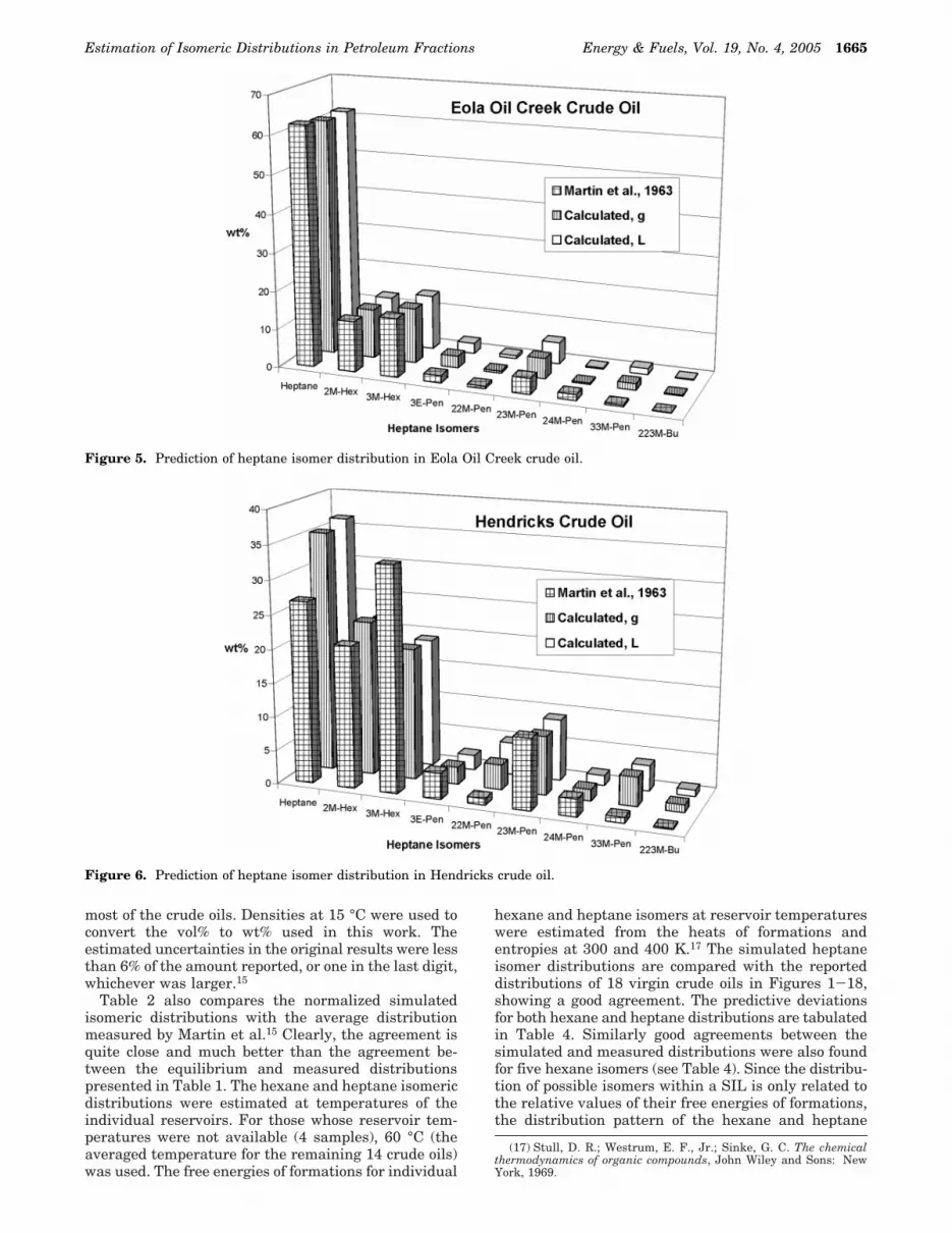
Table 2 also compares the normalized simulatedisomeric distributions with the average distributionmeasured by Martin et al.15 Clearly, the agreement isquite close and much better than the agreement be-tween the equilibrium and measured distributionspresented in Table 1. The hexane and heptane isomericdistributions were estimated at temperatures of theindividual reservoirs. For those whose reservoir tem-peratures were not available (4 samples), 60 °C (theaveraged temperature for the remaining 14 crude oils)was used. The free energies of formations for individual

hexane and heptane isomers at reservoir temperatureswere estimated from the heats of formations andentropies at 300 and 400 K.17 The simulated heptaneisomer distributions are compared with the reporteddistributions of 18 virgin crude oils in Figures 1-18,showing a good agreement. The predictive deviationsfor both hexane and heptane distributions are tabulatedin Table 4. Similarly good agreements between thesimulated and measured distributions were also foundfor five hexane isomers (see Table 4). Since the distribu-tion of possible isomers within a SIL is only related tothe relative values of their free energies of formations,the distribution pattern of the hexane and heptane

(17) Stull, D. R.; Westrum, E. F., Jr.; Sinke, G. C. The chemicalthermodynamics of organic compounds, John Wiley and Sons: NewYork, 1969.

Figure 5. Prediction of heptane isomer distribution in Eola Oil Creek crude oil.

Figure 6. Prediction of heptane isomer distribution in Hendricks crude oil.


isomers in the gas phase were expected to be similar tothose in the liquid phase. Indeed, since the relativevalues of free energy of formations among hexane andheptane isomers in the gas phase were found to be veryclose to those in the liquid phase, similar distributionsin gas and liquid phase were obtained for all 18 crudes(see Figures 1-18 for heptanes). Consequently, only thesimulated isomeric distributions in the gas phase wereused to estimate the prediction errors.

As shown in Table 4, the average absolute errors overall hexane and heptane isomers are less than 3% and1.5% for most of the reported crudes. However, sub-stantial predictive errors are found for the youngercrudes, especially for South Houston, Wafra, and Wilm-ington (see Figure 13, 17, and 18 for heptane isomer

distributions), which were formed during the tertiaryCenozoic Era. The maximum average predictive errorsare 11% and 7% for hexane and heptane isomers,respectively, in Wafra crude (see Table 4). The potentialsignificance of the current approach lies on the fact thatthe approach was able to predict the key isomers (n-hexane, 2-methylpentane, 3-methylpentane for hexaneisomers; n-heptane, 2-methylhexane, 3-methylhexane,and 2,3-dimethylpentane for heptane isomers) with goodconfidence. As shown in Table 4, the relative predictiveerrors were 8.1%, 22.3%, and 16.5% for n-hexane,2-methylpentane, and 3-methylpentane, respectively.Those for n-heptane, 2-methylhexane, 3-methylhexane,and 2,3-dimethylpentane were 5.1%, 7.6%, 20.4%, and15.1%, respectively. The three key isomers made up

Figure 7. Prediction of heptane isomer distribution in Kawkawlin crude oil.

Figure 8. Prediction of heptane isomer distribution in Lee Harrison crude oil.


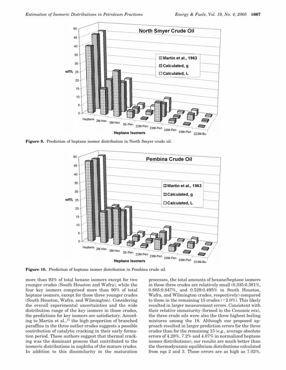
more than 92% of total hexane isomers except for twoyounger crudes (South Houston and Wafra), while thefour key isomers comprised more than 90% of totalheptane isomers, except for those three younger crudes(South Houston, Wafra, and Wilmington). Consideringthe overall experimental uncertainties and the widedistribution range of the key isomers in those crudes,the predictions for key isomers are satisfactory. Accord-ing to Martin et al.,15 the high proportion of branchedparaffins in the three outlier crudes suggests a possiblecontribution of catalytic cracking in their early forma-tion period. These authors suggest that thermal crack-ing was the dominant process that contributed to theisomeric distributions in naphtha of the mature crudes.In addition to this dissimilarity in the maturation

processes, the total amounts of hexane/heptane isomersin these three crudes are relatively small (0.335:0.381%,0.885:0.847%, and 0.529:0.495% in South Houston,Wafra, and Wilmington crudes, respectively) comparedto those in the remaining 15 crudes (>2.0%). This likelyresulted in larger measurement errors. Consistent withtheir relative immaturity (formed in the Cenozoic era),the three crude oils were also the three highest boilingmixtures among the 18. Although our proposed ap-proach resulted in larger prediction errors for the threecrudes than for the remaining 15 (e.g., average absoluteerrors of 4.28%, 7.2% and 4.07% in normalized heptaneisomer distributions), our results are much better thanthe thermodynamic equilibrium distributions calculatedfrom eqs 2 and 3. Those errors are as high as 7.02%,

Figure 9. Prediction of heptane isomer distribution in North Smyer crude oil.

Figure 10. Prediction of heptane isomer distribution in Pembina crude oil.


11.86% and 13.22% for these three crudes, respectively.The good agreements between the simulated and ex-perimental distributions for the mature crude oilssuggest that the proposed method may also be ap-plicable to the predictions of isomer distributions inthermally cracked materials such as coker gas oils.

The purpose of this paper was not to devise a methodfor distributing hexane and heptane isomers but to lookfor a method that would potentially be generally ap-plicable to any SIL, and particularly for heavier SILs.For heavier materials, isolation and identification ofindividual molecules are infeasible. However, the boilingpoint distribution can be obtained experimentally forthe individual SILs during GC-MS measurements re-

gardless of their boiling range. Although the number ofpossible isomeric permutations is very high for largerhydrocarbons, the actual distribution of isomers is notas diverse as might be expected.18 As shown by Martinet al.,15 the distributions of hexane/heptane isomerswere dominated by three or four key isomers thataccounted for 92/90% of total SIL. The distributions ofthese key isomers can be estimated with high accuracyusing current approach. It is possible to use a limitednumber of major isomers to represent a SIL in molecularcharacterizations without losing the intrinsic chemistry

(18) Hood, A.; Clere, R. J.; O’Neal, M. J. J. Inst. Petrol. 1959, 45,168-173.

Figure 11. Prediction of heptane isomer distribution in Ponca City crude oil.

Figure 12. Prediction of heptane isomer distribution in Redwater crude oil.


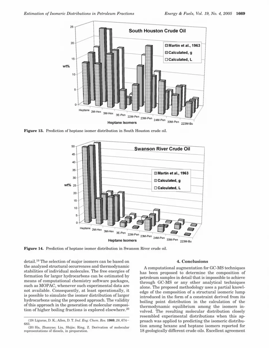
detail.19 The selection of major isomers can be based onthe analyzed structural occurrences and thermodynamicstabilities of individual molecules. The free energies offormation for larger hydrocarbons can be estimated bymeans of computational chemistry software packages,such as MOPAC, whenever such experimental data arenot available. Consequently, at least operationally, itis possible to simulate the isomer distribution of largerhydrocarbons using the proposed approach. The validityof this approach in the generation of molecular composi-tion of higher boiling fractions is explored elsewhere.20

4. ConclusionsA computational augmentation for GC-MS techniques

has been proposed to determine the composition ofpetroleum samples in detail that is impossible to achievethrough GC-MS or any other analytical techniquesalone. The proposed methodology uses a partial knowl-edge of the composition of a structural isomeric lumpintroduced in the form of a constraint derived from itsboiling point distribution in the calculation of thethermodynamic equilibrium among the isomers in-volved. The resulting molecular distribution closelyresembled experimental distributions when this ap-proach was applied to predicting the isomeric distribu-tion among hexane and heptane isomers reported for18 geologically different crude oils. Excellent agreement

(19) Liguras, D. K.; Allen, D. T. Ind. Eng. Chem. Res. 1989, 28, 674-683.

(20) Ha, Zhanyao; Liu, Shijie; Ring, Z. Derivation of molecularrepresentations of diesels, in preparation.

Figure 13. Prediction of heptane isomer distribution in South Houston crude oil.

Figure 14. Prediction of heptane isomer distribution in Swanson River crude oil.


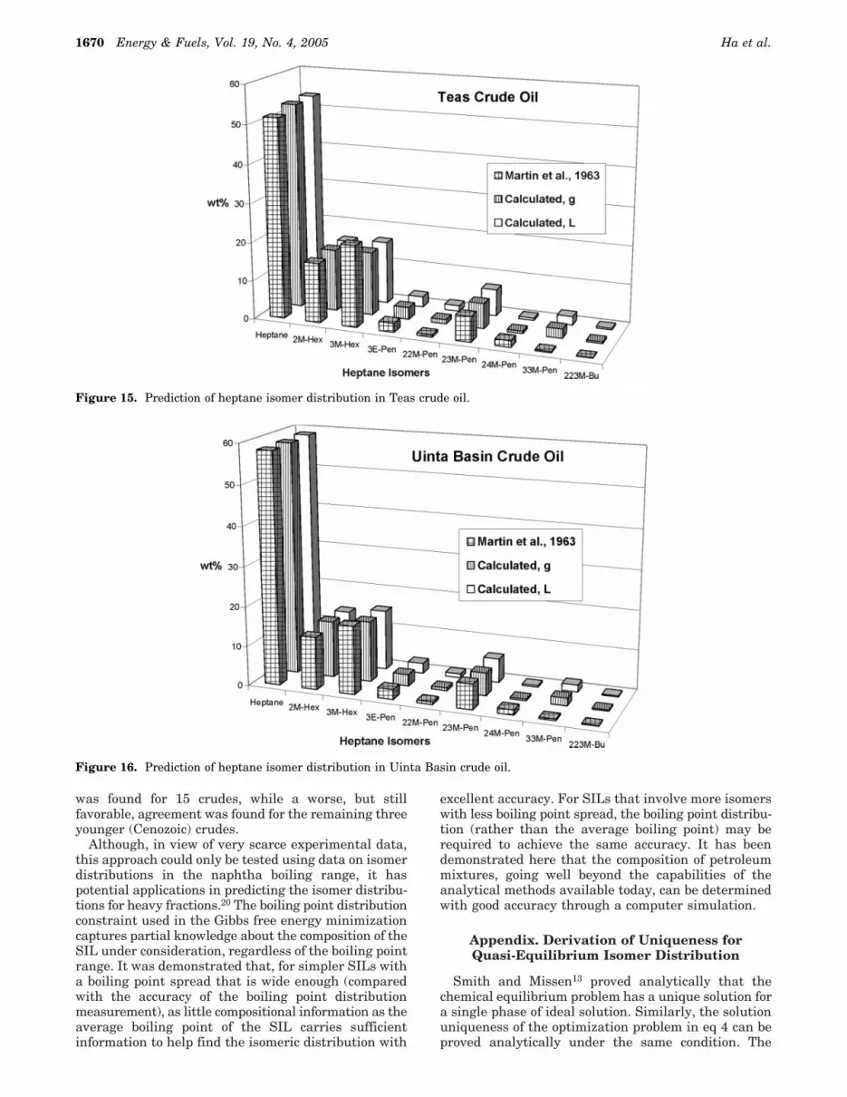
was found for 15 crudes, while a worse, but stillfavorable, agreement was found for the remaining threeyounger (Cenozoic) crudes.

Although, in view of very scarce experimental data,this approach could only be tested using data on isomerdistributions in the naphtha boiling range, it haspotential applications in predicting the isomer distribu-tions for heavy fractions.20 The boiling point distributionconstraint used in the Gibbs free energy minimizationcaptures partial knowledge about the composition of theSIL under consideration, regardless of the boiling pointrange. It was demonstrated that, for simpler SILs witha boiling point spread that is wide enough (comparedwith the accuracy of the boiling point distributionmeasurement), as little compositional information as theaverage boiling point of the SIL carries sufficientinformation to help find the isomeric distribution with

excellent accuracy. For SILs that involve more isomerswith less boiling point spread, the boiling point distribu-tion (rather than the average boiling point) may berequired to achieve the same accuracy. It has beendemonstrated here that the composition of petroleummixtures, going well beyond the capabilities of theanalytical methods available today, can be determinedwith good accuracy through a computer simulation.

Appendix. Derivation of Uniqueness forQuasi-Equilibrium Isomer Distribution

Smith and Missen13 proved analytically that thechemical equilibrium problem has a unique solution fora single phase of ideal solution. Similarly, the solutionuniqueness of the optimization problem in eq 4 can beproved analytically under the same condition. The

Figure 15. Prediction of heptane isomer distribution in Teas crude oil.

Figure 16. Prediction of heptane isomer distribution in Uinta Basin crude oil.


constrained optimization problem can be solved by theLagrange Multiplier method. The Lagrangian functionis defined as

Minimizing F with respect to x and λ results in a setof nonlinear equations

and constraints:

Substituting the derivatives of eq 1 into eq A-2 andsolving for xi, we obtain

Therefore, minimizing the Lagrangian function is re-duced to solving the following set of nonlinear equations

and

Mathematically, eqs A-5 and A-6 can be written as

Figure 17. Prediction of heptane isomer distribution in Wafra crude oil.

Figure 18. Prediction of heptane isomer distribution in Wilmington crude oil.

F(x,λ) ) ∆Gn0 + λ1(1 - ∑ xi) +

λ2(BPlump - ∑ xi BPi) (A-1)

∂F∂xi

)∂∆Gn

0

∂xi- λ1 - λ2BPi ) 0 i ) 1, 2, ‚‚‚, N (A-2)

∂F∂λj

) 0 j ) 1, 2 (A-3)

xi ) e(λ1+λ2BPi-∆G i0-RT)/RT (A-4)

∑i)1

N

e(λ1+λ2BPi-∆G i0-RT)/RT - 1 ) 0 (A-5)

∑i)1

N

BPi(e(λ1+λ2BPi-∆G i

0-RT)/RT) - BPlump ) 0 (A-6)


where t1 ) λ1/RT, t2 ) λ2/RT, ai ) -(1 + ∆Gio/RT),

bi ) BPi, and c ) BPlump.The solution to the optimization problem is (λ1, λ2) )

f(T, t1, t2), such that

Assuming Z1 and Z2 are two roots of (F)(t):

Let

If multiple solutions exist, eqs A-10 and A-11 give

Then

and

With the stoichiometric constraint ∑i)1N eai+ê1+biê2 ) 1, eq

A-13 can be rearranged to give

Substituting eq A-15 into A-14 yields

Physically, 0 < exp(ai + ê1 + biê2) < 1; and bi ) BPi (K)> 0 for all hydrocarbons. Thus,

Therefore, to satisfy eqs A-15 and A-16, the followingequation has to be true

One can conclude, then, that multiple solutions do notexist. The nonlinear eqs A-5 and A-6 have a uniquesolution of the Lagrange multiplier (λ1 and λ2). Conse-quently, the composition xi determined by eq A-4 is alsounique.

Acknowledgment. Partial funding for NCUT hasbeen provided by the Canadian Program for EnergyResearch and Development (PERD), the Alberta Re-search Council (ARC) and the Alberta Energy ResearchInstitute (AERI). The authors thank Professor R. W.Missen (University of Toronto) and Professor W. R.Smith (University of Ontario Institute of Technology)for their valuable comments.EF049712R

Tab

le4.

Pre

dic

tion

Dev

iati

ons

(Cal

cula

ted

-M

easu

red

)fo

rN

orm

aliz

edD

istr

ibu

tion

ofH

exan

e/H

epta

ne

Isom

ers

(wt%

)

cru

de/is

omer

sH

ex.

2M-P

en.

3M-P

en.

22M

-Bu

t.23

M-B

ut.

ave

abs

in5

isom

ers

Hep

.2M

-Hex

.3M

-Hex

.3E

-Pen

.22

M-P

en.

23M

-Pen

.24

M-P

en.

33M

-Pen

.22

3M-B

ut.

ave

abs

in9

isom

ers

Ali

da2.

378

-5.

898

0.33

71.

683

1.50

02.

359

1.70

70.

987

-5.

266

0.87

00.

453

-0.

234

-0.

832

1.99

50.

320

1.40

7B

ever

Lod

ge0.

966

-5.

434

2.03

01.

058

1.38

12.

174

-0.

008

0.85

8-

3.28

51.

057

0.03

80.

711

-1.

184

1.60

10.

213

0.99

5D

ariu

s2.

063

-3.

624

-0.

883

1.11

81.

326

1.80

30.

768

-1.

339

-4.

043

2.05

70.

376

0.94

9-

0.86

61.

761

0.33

91.

389

Eol

aM

clis

h2.

680

-7.

198

0.53

51.

843

2.14

02.

879

2.15

00.

354

-5.

535

0.02

70.

570

1.10

9-

0.91

31.

958

0.28

11.

433

Eol

aoi

lcre

ek-

0.00

1-

5.08

33.

170

0.62

61.

288

2.03

4-

0.99

9-

0.44

3-

0.97

61.

173

-0.

111

1.17

2-

1.18

91.

244

0.12

80.

826

Hen

dric

ks8.

748

-4.

326

-9.

515

4.09

50.

999

5.53

78.

607

1.86

213

.624

-1.

311

2.73

0-

1.78

6-

0.90

23.

473

0.95

13.

916

Kaw

kaw

lin

-1.

839

-2.

566

4.68

9-

0.09

7-

0.18

71.

875

-1.

081

-0.

671

1.06

10.

833

-0.

110

0.22

5-

0.36

60.

129

-0.

020

0.50

0L

eeH

arri

son

6.38

8-

4.98

1-

4.51

54.

048

-0.

941

4.17

44.

115

0.80

3-

5.12

3-

0.14

11.

251

-3.

767

-0.

342

2.68

40.

520

2.08

3N

orth

Sm

yer

7.50

2-

9.58

7-

5.11

93.

838

3.36

65.

882

5.27

53.

185

-8.

860

-0.

670

1.37

3-

3.26

3-

0.62

32.

892

0.69

12.

981

Pem

bin

a2.

654

-5.

698

0.03

61.

904

1.10

42.

279

-0.

049

-0.

081

-3.

485

1.07

50.

323

1.50

8-

2.16

22.

430

0.44

11.

284

Pon

caci

ty1.

333

-5.

815

1.63

71.

178

1.66

62.

326

0.24

20.

967

-2.

721

0.90

40.

123

-0.

227

-0.

876

1.39

90.

188

0.85

0R

edw

ater

4.75

2-

7.53

8-

2.29

02.

636

2.44

03.

931

2.55

72.

243

-5.

819

-0.

853

0.62

7-

0.15

9-

1.10

42.

160

0.34

81.

763

Sou

thH

oust

on-

3.89

811

.257

3.66

60.

389

-11

.413

6.12

52.

214

10.3

780.

329

-3.

732

4.92

110

.270

-4.

577

1.41

7-

0.67

94.

280

Sw

anso

nR

iver

3.06

7-

7.12

20.

526

2.36

21.

168

2.84

9-

0.48

40.

795

-1.

342

0.20

30.

737

0.15

6-

2.75

82.

350

0.34

31.

019

Tea

s2.

963

-6.

502

-0.

094

2.00

21.

631

2.63

81.

503

0.52

4-

4.70

20.

762

0.47

50.

005

-1.

080

2.15

20.

361

1.28

5U

inta

Bas

in3.

697

-9.

571

0.76

32.

658

2.45

33.

828

0.21

51.

018

-1.

908

0.40

40.

070

-0.

613

-0.

900

1.53

70.

176

0.76

0W

afra

18.4

261.

834

-25

.881

7.90

8-

2.28

811

.267

15.5

573.

864

19.8

55-

3.22

75.

664

-7.

639

-1.

660

5.19

52.

101

7.19

6W

ilm

ingt

on6.

996

-4.

391

-7.

097

3.34

71.

145

4.59

55.

587

7.37

8-

5.66

2-

4.06

71.

618

-7.

414

-1.

179

3.06

80.

672

4.07

2A

RD

ain

15cr

ude

oils

0.08

10.

223

0.16

54.

550

0.54

7N

/A0.

051

0.07

60.

204

0.43

41.

156

0.15

10.

630

5.23

63.

683

N/A

aA

ve.

Rel

.D

ev.

)∑

[|pre

dict

ed-m

easu

red|/

mea

sure

d]/1

5;S

outh

Hou

ston

,W

afra

,an

dW

ilm

ingt

onar

eex

clu

ded

F1 ) ∑ exp(ai + t1 + bit2) - 1 (A-7)

F2 ) ∑ bi exp(ai + t1 + bit2) - c (A-8)

(F)(t) ) (F1F2

) ) 0 (A-9)

F(Z1) - F(Z2) ) F′(ê)(Z1 - Z2) ) 0 (A-10)

Z1 - Z2 ) (m1m2

) (A-11)

(∑ eai+ê1+biê2 ∑ bieai+ê1+biê2

∑ bieai+ê1+biê2 ∑ bi

2eai+ê1+biê2 )(m1m2 ) ) 0 (A-12)

∑ m1eai+ê1+biê2 + ∑ m2bie

ai+ê1+biê2 ) 0 (A-13)

∑ m1bieai+ê1+biê2 + ∑ m2bi

2eai+ê1+biê2 ) 0 (A-14)

m1 ) - m2 ∑ bieai+ê1+biê2 (A-15)

m2 ∑ bi2eai+ê1+biê2 - m2( ∑ bie

ai+ê1+biê2)2 ) 0 (A-16)

∑ bi2eai+ê1+biê2 * ( ∑ bie

ai+ê1+biê2)2

m1 ) m2 ) 0 (A-17)


estimation of isomeric distributions in petroleum fractions

Documents