energy-efficient routing schemes for underwater acoustic networks

1754 IEEE JOURNAL ON SELECTED AREAS IN COMMUNICATIONS, VOL. 26, NO. 9, DECEMBER 2008

Energy-Efficient Routing Schemes forUnderwater Acoustic Networks

Michele Zorzi, Fellow, IEEE, Paolo Casari, Member, IEEE,Nicola Baldo, Student Member, IEEE, and Albert F. Harris III

Abstract—Interest in underwater acoustic networks has grownrapidly with the desire to monitor the large portion of the worldcovered by oceans. Fundamental differences between underwateracoustic propagation and terrestrial radio propagation may callfor new criteria for the design of networking protocols. Inthis paper, we focus on some of these fundamental differences,including attenuation and noise, propagation delays, and thedependence of usable bandwidth and transmit power on distance(which has not been extensively considered before in protocoldesign studies). Furthermore, the relationship between the energyconsumptions of acoustic modems in various modes (i.e., trans-mit, receive, and idle) is different than that of their terrestrialradio counterparts, which also impacts the design of energy-efficient protocols. The main contribution of this work is anin-depth analysis of the impacts of these unique relationships.We present insights that are useful in guiding both protocoldesign and network deployment. We design a class of energy-efficient routing protocols for underwater sensor networks basedon the insights gained in our analysis. These protocols aretested in a number of relevant network scenarios, and shown tosignificantly outperform other commonly used routing strategiesand to provide near optimal total path energy consumption.Finally, we implement in ns2 a detailed model of the underwateracoustic channel, and study the performance of routing choiceswhen used with a simple MAC protocol and a realistic PHYmodel, with special regard to such issues as interference andmedium access.

Index Terms—Underwater acoustic networks, routing schemes,performance analysis, characteristic distance, energy-efficientprotocol design.

I. INTRODUCTION

THE GROWING interest in the design of underwaterad hoc networks is driven by the desire to provide

autonomous support for many activities, such as monitoringof equipment (e.g., underwater oil mining rigs) and naturalevents (e.g., underwater seismic activity). Radio technologyis unsuitable for underwater environments due to its poorpropagation through water. As a result, acoustic modems arethe current technology of choice for these scenarios [1]–[3].

Underwater protocol design has drawn the attention of thenetworking research community only very recently, and as aresult little work exists in this area. While considerable work

Manuscript received March 1, 2008; revised August 31, 2008. This workhas been partially supported by the NATO Undersea Research Center undercontract no. 40480700 (ref. NURC-010-08). Part of this work was presentedat the IEEE SECON 2007 conference.

M. Zorzi, P. Casari and N. Baldo are with the Department of Infor-mation Engineering, University of Padova (e-mail: {zorzi,casarip,baldo}@dei.unipd.it).

A. Harris is with the Center for Remote Sensing of Ice Sheets, Universityof Kansas (e-mail: [email protected]).

Digital Object Identifier 10.1109/JSAC.2008.081214.

has been done at the physical layer [4]–[6] and in buildingdevices [7], work at higher layers of the protocol stack isjust beginning [1]–[3]. There have been a few proposals forMAC-layer schemes to handle increased delay while stillproviding reliability or energy efficiency [8]–[14]. This workhas shown that the differences in propagation properties forunderwater acoustic signals may greatly affect the optimalchoices for MAC-layer protocols, and that there is still muchroom for innovation. Early work on routing and transportlayer protocols has focused on dealing with the long delayspresent for acoustic signals while providing energy-efficientreliability [15]–[18], but has not included important propaga-tion factors such as the bandwidth-distance and power-distancerelationships, which affect energy consumption through bothpower and rate, nor specific modem energy consumptioncharacteristics.

Energy-efficient routing in terrestrial networks has beenwell studied and a large number of algorithms have been pro-posed [19]–[25]. Some of these algorithms deal with increas-ing the hop-count, thereby decreasing hop-distance, whichmay result in lower total energy consumption. Other worksdeal with selecting paths that allow the maximum number ofnodes to transition into a low-power sleep state. The relation-ship between the total energy consumption along a straightroute and the number of hops has been explored in [26],where it is also shown that in this case the minimum energypath consists of equally spaced relays, where the optimal hopdistance (called characteristic distance in the paper) can beanalytically computed from the propagation characteristics anda first-order energy model. The implications this result has onthe design of routing schemes, not explored in [26], have beenconsidered in [27], where forwarding techniques are designedin the context of energy and traffic balancing. The paper thatcomes closest to our approach is [28], where a routing protocolis designed in which a relay is chosen as the node closest tothe optimal relay position determined in [26].

A critical component for the development of routing proto-cols is the understanding of the impacts of channel properties,such as path loss and bandwidth, on key metrics used forrouting, such as energy consumption and delay. While work oncapacity and bandwidth for terrestrial radio networks is wellknown [29], no equivalent work is available for underwateracoustic networks. Preliminary link capacity results werepresented in a very recent paper [30], that defines the impactof the bandwidth-distance relationship on link bit rate andpower but does not directly extend to a multihop or multi-flow viewpoint.

0733-8716/08/$25.00 c© 2008 IEEE

Authorized licensed use limited to: ELETTRONICA E INFORMATICA PADOVA. Downloaded on December 3, 2008 at 06:34 from IEEE Xplore. Restrictions apply.

ZORZI et al.: ENERGY-EFFICIENT ROUTING SCHEMES FOR UNDERWATER ACOUSTIC NETWORKS 1755

In the present paper, we develop algorithms to minimizethe total path energy consumption in an underwater acousticnetwork by leveraging observations made through a studyof the impacts of the propagation characteristics of acousticsignals. To our knowledge, this is the first attempt to performsuch a study for underwater acoustic networks. Taking theseeffects explicitly into account provides a much more realisticstudy, and leads to different design criteria, whereas traditionalapproaches lead to inefficient solutions. When consideringa different scenario (underwater vs. terrestrial), where therules of acoustic propagation are significantly different fromthose for radio, it remains to be determined whether thedesign criteria and the results reported for terrestrial networksstill apply. For example, in underwater acoustics, where therelationship between the relay displacement compared to theoptimal position and the energy consumption is significantlyasymmetric (i.e., choosing longer- rather than shorter-than-optimal hops leads to significantly different degrees of energysuboptimality), the symmetric approach of [28] does notnecessarily lead to good solutions. In addition, the analysesreported in [26]–[28] tend to consider rather simplified net-work deployments, or do not study in detail the suboptimalityeffects related to the random node deployments.

The main contribution of this work is the first in-depthanalysis of the effects of all the main characteristics ofunderwater acoustic signal propagation and of the acousticmodem energy consumption profiles on energy-efficient rout-ing design. To this end, we first present in Section II thecharacteristics of underwater acoustic channels (highlightingespecially the bandwidth-distance relationship), the energyconsumption profile of current acoustic modems, and therelevant computations of delay and energy consumption overan acoustic link, which provide the basis for the analysis ofmultihop schemes in an underwater scenario and the designof proper protocols. To provide protocol design guidelines,we analyze the routing performance based on hop-distance,delay, and energy consumption. We first develop in Section IIIa simple analysis to test the effect of hop length and nodedensity on the statistics of the path energy consumption.Based on the key observation that an optimal hop distanceexists, in Section IV we develop routing algorithms whererelays are chosen so as to provide a hop length close to theoptimum, and compare them with standard routing approachessuch as shortest path and greedy minimum energy, as wellas the centrally computed minimum-energy benchmark. Bymeans of simple simulations, we show that the overall pathenergy consumption for the routes found by the proposedalgorithms is always close to the optimum and significantlybetter than those obtained with the other schemes. For a morerealistic evaluation, we also implement a complete protocolsuite (PHY, MAC, routing and application) together with theunderwater channel model in ns2, and use this model to testthe impact of some issues expected in real systems, suchas interference and congestion, on the performance of ourrouting protocol. The numerical results again show that ourapproach outperforms other strategies, achieving better trade-offs between energy, throughput and delay. Finally, Section Voutlines some conclusions and future directions.

II. BASIC FEATURES OF UNDERWATER PROPAGATION

This section characterizes the unique bandwidth-distance re-lationship, signal-to-noise ratio (SNR), and propagation delayin an underwater acoustic channel. For a more complete de-scription of underwater channel characteristics see Urick [31]and Stojanovic [30]. The energy consumption characteristicsof a typical acoustic modem, as well as the relevant linkbudget equations to be used in the computation of path energyconsumption, are also described.

We stress that all these features of acoustic propagationand devices significantly affect the performance of a protocol.Unlike past efforts, in which only a subset of these effectswere considered, the protocol design proposed in this paper isthe first to explicitly include all of them.

A. Attenuation and propagation delay

The attenuation factor A(�, f) of an underwater acousticchannel for a distance � and a frequency f can be empiricallymodeled in terms of the spreading loss, the absorption loss,and the spreading coefficient k, as follows [31]:

10 logA(�, f) = k · 10 log � + � · 10 log a(f), (1)

where the first term is the spreading loss and the second termis the absorption loss. The spreading coefficient defines thegeometry of the propagation (i.e., k = 1 is cylindrical, k = 2is spherical, and k = 1.5 is practical spreading [31]).

Thorp’s formula (also empirically derived) can be used toexpress the absorption coefficient a(f) for frequencies abovea few hundred Hz as follows [32]:

10 log a(f) = 0.11f2

1+f2 + 44f2

4100+f2 + 2.75f2

104 + 0.003, (2)

where a(f) is given in dB/km and f is in kHz. The absorptioncoefficient is the major factor that limits the maximum usablebandwidth at a given distance, as it increases very rapidly withfrequency. This model describes the attenuation on a single,unobstructed propagation path. If a tone of frequency f andpower P is transmitted over a distance �, the received signalpower will be P/A(�, f).

The underwater acoustic propagation speed c in m/s hasbeen shown to depend on a number of factors, includingthe water depth and its temperature and salinity [31]. Forthe purposes of this paper, also in view of the rather weakdependence of c on these factors, we assume c = 1500 m/s,which is a commonly considered average value. The use ofmore sophisticated models, e.g., to relate the depth of anunderwater link to the corresponding propagation delay, is leftfor future study, although we do not expect them to provideany significant additional insight on routing, compared to whatis discussed in the present paper.

B. Transmission Distance and Bandwidth

For typical terrestrial radio environments, shorter trans-mission distances lead to either the ability to use lowerpower (due to less signal attenuation), or the ability to usehigher bit rates (due to a higher signal-to-noise ratio), butthe bandwidth available remains constant. For the underwateracoustic environment, however, not only do these two effects



0 10 20 30 40 50 60

−160

−140

−120

−100

−80

−60

Frequency , [kHz]

1/A

N fa

ctor

, [l

og s

cale

]

d = 0.1 kmd = 1 kmd = 5 kmd = 10 kmd = 25 kmd = 50 kmd = 75 kmd = 100 km

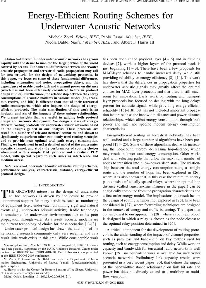
Fig. 1. 1/AN factor vs. frequency, for various link distances

exist but the bandwidth available increases as the distancedecreases, a fundamental difference between acoustic channelsand radio channels. This is due to the fact that both signalpropagation and noise in underwater environments show asignificant dependence on frequency [31], unlike in wirelessradio where the noise at the receiver is well approximated aswhite, and frequency selectivity, though present, is usually lesspronounced [33]. The combination of these two effects, repre-sented by the attenuation A(�, f) and the noise power spectraldensity N(f), characterizes the communications behavior inthe frequency domain.

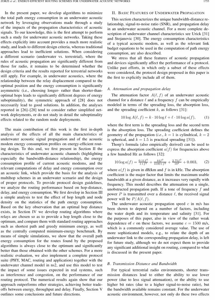
The complex distance–bandwidth relationship is best expli-cated by considering the 1/AN factor (which is proportionalto the SNR at the receiver) across frequencies for differentdistances (Figure 1). For a given value of the distance �,there exists a frequency that corresponds to the best attenua-tion/noise combination for the channel, and the bandwidth canthen be defined using some criterion. In [30], two exampleswere given, i.e., a heuristic 3 dB bandwidth definition and anoptimal capacity-based bandwidth definition. In both cases,as distances decrease, not only do the maxima in the curveschange (different attenuation), but also the widths of the curveschange (different bandwidth). This corresponds to a broaderbandwidth spectrum available to the shorter links, allowing alarger link capacity. Figure 2 shows the best frequency as afunction of the link distance �, with the bars representing theavailable bandwidth.

Following the theoretical analysis in [30], for a givenperformance objective (target SNR) the usable bandwidthB(�) and the required transmit power Pt(�) can be calculatedas a function of the transmitter-receiver distance, �. Suchrelationships can also be approximated by empirical formulasof the form

B(�) = b�−β, Pt(�) = p�π (3)

where the positive parameters b, β, p, π depend on the targetSNR. More details can be found in [30].

Note that the theoretical behavior illustrated in (3), wherethe transmit power and the transmission bandwidth can beadjusted to any value, is not available in current devices, andmay present significant difficulties even in next generationmodems. The analysis that we present, however, has signifi-

0

5

10

15

20

25

30

35

40

45

50

55

0 1000 2000 3000 4000 5000

Fre

quen

cy (

kHz)

Distance (m)

Fig. 2. Optimal frequency vs. distance, and 3-dB bandwidth (bars)

cant theoretical value both as a bound to what can be achievedand as a motivation for more capable devices, e.g., based onsoftware-programmable waveform design.

C. Energy consumption of acoustic modems

For each specific acoustic modem interface, the receiveenergy is fixed (as an example, we consider here the WHOImicro-modem [7] that has a few Watts of receive power). Thetransmit energy of the WHOI micro-modem has a maximumtransmit power of 50 W that can achieve over 190 dB re μPaof acoustic pressure (acoustic pressure is the equivalent of RFpower for underwater environments) at distances up to 4 km.It has a 10 W minimum transmit power level, potentially pro-viding a 40 W dynamic range for power control.1 Because thisrange represents 80% of the maximum energy consumption intransmit mode, transmit power control has the potential to havea large impact on energy consumption. By way of contrast, thedynamic range for power control in current radio modems ison the order of 90 mW and only represents a small percentageof the maximum energy consumption in transmit mode [34].Additionally, the difference in energy consumption betweenreceive and idle modes for acoustic modems can be an orderof magnitude or more [2], [7], whereas for radio modems theyare nearly identical [34], an aspect that can be exploited in thedesign of energy-efficient topology control schemes [35].

D. Computation of the hop delay and energy consumption

The attenuation equations of Section II-A and [30] providea means to compute the received acoustic power (and conse-quently the SNR) for an underwater link of a given length.In order to properly relate these computations with the energyconsumption associated to one hop (which includes both thetransmit and the receive energy at the two ends of the link),we must take into account modem specifications such as thosediscussed in Section II-C, as well as the proper conversionbetween the level of radiated acoustic power (expressed in dBre μPa) and the corresponding electrical power consumption inthe device (in Watts). In addition, the bandwidth calculations

1Note that power control is not currently implemented in the WHOI micro-modem, but is expected to be considered for future versions [7].



of Section II-B make it possible to compute the transmissiontime, which affects both the energy consumption and the delay.

More precisely, in the presence of power control thetransmit energy consumption depends on the distance to becovered, as longer links require more power in general.2

Based on the attenuation equations, and following the analysisof [30], the acoustic power that needs to be radiated in orderto meet some quality threshold at the receiver depends ondistance.

Assuming the use of BPSK,3 and the transmission ofpackets of length L, the transmit power level required toachieve a target packet error rate (PER) Πtgt can be foundby inverting the BPSK error equations. For example, underthe assumption of independent channel errors, PER can befound as

Πpkt = 1 −(

1 − 12erfc

√ξSNR

)L

, (4)

where SNR is the signal-to-noise ratio at the receiver, andξ is a penalty factor that accounts for signal processinginefficiencies at the receiver. In order for (4) to be equal toΠtgt , the following condition on the transmit power must hold:

Pt(�) =χ

ξB(�)N(f0(�))A(�, f0(�)) SNRtgt , (5)

where f0(�) is the optimal transmit frequency at a givendistance � [30] (see also Figure 2), B(�) is found according to(3), an analogous approximation is used for f0(�), and SNRtgt

is given by

SNRtgt =(erfc−1(2 − 2(1 − Πtgt )1/L)

)2

. (6)

Note that in (5) both noise and attenuation are calculated atf0(�) and approximated as constant over the whole bandwidth.Also, (5) includes a margin, χ, so that the average SNR at thereceiver is larger than the minimum required by (4), in orderto protect the system from random fluctuations. In order totranslate acoustic power into electrical power the followingempirical relation is applied [31]:

P elt (�) = Pt(�) · 10−17.2/η , (7)

where 10−17.2 is the conversion factor from acoustic powerin dB re μPa to electrical power in Watt, and η is the overallefficiency of the electronic circuitry (power amplifier andtransducer).

Unlike the transmit power, the receive power Pr is inde-pendent of distance, and rather depends on the complexity ofthe receive operations (e.g., whether coherent detection and/orequalization are performed). Other fixed costs (such as theelectrical power required to keep systems active) are neglectedhere, as they cause minimal variations of the overall energyconsumption.

2In order to evaluate the greatest possible gain, in this paper we assumecontinuous transmit power control, whose performance provides an upperbound to what may be achievable by practical devices where there is typicallyonly a discrete set of possible power levels for transmission.

3BPSK is one of the transmission modes available in the WHOI micro-modem [7], along with FH-FSK. The methodology explained here can beextended to any modulation scheme in a straightforward manner, by justreplacing (4) with the appropriate error rate expression.

Therefore, for a given SNR requirement, the total energyconsumption associated to a single hop of length � can becomputed as the total (transmit plus receive) power, equal toPr + P el

t (�), times the duration of time the modems need tobe operated, which is equal to the transmission time of thepacket, i.e., L

αB(�) , where L is the packet size in bits, B(�) isthe bandwidth available (which depends on the link distance),and α is the bandwidth efficiency of the modulation in bps/Hz.

Finally, the hop delay and energy consumption can beexpressed as4

Δhop(�) =L

αB(�)+

�

c, Ehop(�) =

(Pr + P elt (�))L

αB(�)(8)

The delay and energy consumption associated to a completemulti-hop path are computed by adding the delays and energyconsumptions of the individual hops. In the following, we willassume L = 256 bytes, Πtgt = 0.01, ξ = −10 dB, χ =10 dB, η = 0.25 and Pr = 2 W, unless differently stated.

III. ANALYSIS OF PATH DELAY AND ENERGY

CONSUMPTION

To evaluate the impact that the characteristics of acousticpropagation and devices described in the previous section haveon routing algorithm design, we first study the effects ofnode density and hop length on end-to-end delay and energyconsumption in simple networks. To calculate the bit rate andpower for a given distance, we use the models summarized inSection II. The goal of our evaluation is to gain insights thatcan be used to design a routing algorithm to minimize energyconsumption for underwater networks.

A. Linear topologies

As a first step, we consider the simplest scenario of a lineartopology, where all nodes are placed on a straight line, andstudy how the overall path delay and energy consumption de-pend on the number of nodes between source and destination.

More specifically, consider a one-dimensional axis withcoordinate x. The source and final destination are placed inpositions x0 = 0 and xn = D, respectively, with n − 1intermediate nodes at xi, i = 1, . . . , n−1, with xi < xi+1, i =0, . . . , n − 1. The resulting n-hop path has total delay andenergy consumption

Δpath(n) =n∑

i=1

Δhop(�i), Epath(n) =n∑

i=1

Ehop(�i) (9)

where �i = xi − xi−1 is the distance covered by the i-th hop.If the hops are all of the same length, we have �i = D/n

and

Δpath(n) =nL

αB(

Dn

) +D

c,

Epath(n) =n(Pr + P el

t

(Dn

))L

αB(

Dn

) (10)

4Note that it may be appropriate to add to the delay term a componentwhich accounts for processing delay at each hop. This would be a constantterm which does not essentially affect the behavior of the delay curves, andis ignored here for simplicity.



0 5 10 15 20 25 300

10

20

30

40

50

60

70

80

90

Number of relays

Del

ay [s

]

Dtot

= 10 km

Dtot

= 100 km

Variable bandwidthAny of WHOI MM bands, 50 km

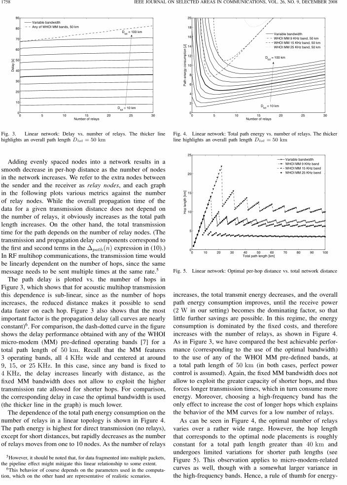
Fig. 3. Linear network: Delay vs. number of relays. The thicker linehighlights an overall path length Dtot = 50 km

Adding evenly spaced nodes into a network results in asmooth decrease in per-hop distance as the number of nodesin the network increases. We refer to the extra nodes betweenthe sender and the receiver as relay nodes, and each graphin the following plots various metrics against the numberof relay nodes. While the overall propagation time of thedata for a given transmission distance does not depend onthe number of relays, it obviously increases as the total pathlength increases. On the other hand, the total transmissiontime for the path depends on the number of relay nodes. (Thetransmission and propagation delay components correspond tothe first and second terms in the Δpath(n) expression in (10).)In RF multihop communications, the transmission time wouldbe linearly dependent on the number of hops, since the samemessage needs to be sent multiple times at the same rate.5

The path delay is plotted vs. the number of hops inFigure 3, which shows that for acoustic multihop transmissionthis dependence is sub-linear, since as the number of hopsincreases, the reduced distance makes it possible to senddata faster on each hop. Figure 3 also shows that the mostimportant factor is the propagation delay (all curves are nearlyconstant)6. For comparison, the dash-dotted curve in the figureshows the delay performance obtained with any of the WHOImicro-modem (MM) pre-defined operating bands [7] for atotal path length of 50 km. Recall that the MM features3 operating bands, all 4 KHz wide and centered at around9, 15, or 25 KHz. In this case, since any band is fixed to4 KHz, the delay increases linearly with distance, as thefixed MM bandwidth does not allow to exploit the highertransmission rate allowed for shorter hops. For comparison,the corresponding delay in case the optimal bandwidth is used(the thicker line in the graph) is much lower.

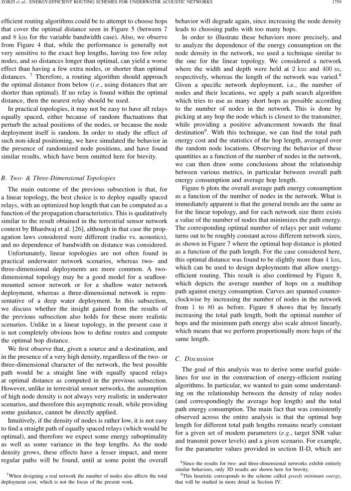
The dependence of the total path energy consumption on thenumber of relays in a linear topology is shown in Figure 4.The path energy is highest for direct transmission (no relays),except for short distances, but rapidly decreases as the numberof relays moves from one to 10 nodes. As the number of relays

5However, it should be noted that, for data fragmented into multiple packets,the pipeline effect might mitigate this linear relationship to some extent.

6This behavior of course depends on the parameters used in the computa-tion, which on the other hand are representative of realistic scenarios.

0 5 10 15 20 25 300

2

4

6

8

10

12

14

16

18

20

Number of relays

Pat

h en

ergy

con

sum

ptio

n [J

]

Dtot

= 10 km

Dtot

= 100 km

Variable bandwidthWHOI MM 9 KHz band, 50 kmWHOI MM 15 KHz band, 50 kmWHOI MM 25 KHz band, 50 km

Fig. 4. Linear network: Total path energy vs. number of relays. The thickerline highlights an overall path length Dtot = 50 km

0 10 20 30 40 50 60 70 80 90 1000

5

10

15

20

25

Total path length [km]

Hop

leng

th [k

m]

Variable bandwidthWHOI MM 9 KHz bandWHOI MM 15 KHz bandWHOI MM 25 KHz band

Fig. 5. Linear network: Optimal per-hop distance vs. total network distance

increases, the total transmit energy decreases, and the overallpath energy consumption improves, until the receive power(2 W in our setting) becomes the dominating factor, so thatlittle further savings are possible. In this regime, the energyconsumption is dominated by the fixed costs, and thereforeincreases with the number of relays, as shown in Figure 4.As in Figure 3, we have compared the best achievable perfor-mance (corresponding to the use of the optimal bandwidth)to the use of any of the WHOI MM pre-defined bands, ata total path length of 50 km (in both cases, perfect powercontrol is assumed). Again, the fixed MM bandwidth does notallow to exploit the greater capacity of shorter hops, and thusforces longer transmission times, which in turn consume moreenergy. Moreover, choosing a high-frequency band has theonly effect to increase the cost of longer hops which explainsthe behavior of the MM curves for a low number of relays.

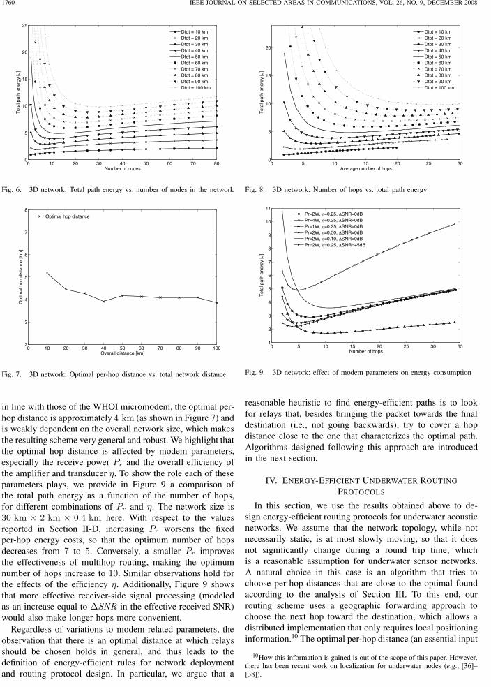
As can be seen in Figure 4, the optimal number of relaysvaries over a rather wide range. However, the hop lengththat corresponds to the optimal node placements is roughlyconstant for a total path length greater than 40 km andundergoes limited variations for shorter path lengths (seeFigure 5). This observation applies to micro-modem-relatedcurves as well, though with a somewhat larger variance inthe high-frequency bands. Hence, a rule of thumb for energy-



efficient routing algorithms could be to attempt to choose hopsthat cover the optimal distance seen in Figure 5 (between 7and 8 km for the variable bandwidth case). Also, we observefrom Figure 4 that, while the performance is generally notvery sensitive to the exact hop lengths, having too few relaynodes, and so distances longer than optimal, can yield a worseeffect than having a few extra nodes, or shorter than optimaldistances. 7 Therefore, a routing algorithm should approachthe optimal distance from below (i.e., using distances that areshorter than optimal). If no relay is found within the optimaldistance, then the nearest relay should be used.

In practical topologies, it may not be easy to have all relaysequally spaced, either because of random fluctuations thatperturb the actual positions of the nodes, or because the nodedeployment itself is random. In order to study the effect ofsuch non-ideal positioning, we have simulated the behavior inthe presence of randomized node positions, and have foundsimilar results, which have been omitted here for brevity.

B. Two- & Three-Dimensional Topologies

The main outcome of the previous subsection is that, fora linear topology, the best choice is to deploy equally spacedrelays, with an optimized hop length that can be computed as afunction of the propagation characteristics. This is qualitativelysimilar to the result obtained in the terrestrial sensor networkcontext by Bhardwaj et al. [26], although in that case the prop-agation laws considered were different (radio vs. acoustics),and no dependence of bandwidth on distance was considered.

Unfortunately, linear topologies are not often found inpractical underwater network scenarios, whereas two- andthree-dimensional deployments are more common. A two-dimensional topology may be a good model for a seafloor-mounted sensor network or for a shallow water networkdeployment, whereas a three-dimensional network is repre-sentative of a deep water deployment. In this subsection,we discuss whether the insight gained from the results ofthe previous subsection also holds for these more realisticscenarios. Unlike in a linear topology, in the present case itis not completely obvious how to define routes and computethe optimal hop distance.

We first observe that, given a source and a destination, andin the presence of a very high density, regardless of the two- orthree-dimensional character of the network, the best possiblepath would be a straight line with equally spaced relaysat optimal distance as computed in the previous subsection.However, unlike in terrestrial sensor networks, the assumptionof high node density is not always very realistic in underwaterscenarios, and therefore this asymptotic result, while providingsome guidance, cannot be directly applied.

Intuitively, if the density of nodes is rather low, it is not easyto find a straight path of equally spaced relays (which would beoptimal), and therefore we expect some energy suboptimalityas well as some variance in the hop lengths. As the nodedensity grows, these effects have a lesser impact, and moreregular paths will be found, until at some point the overall

7When designing a real network the number of nodes also affects the totaldeployment cost, which is not the focus of the present work.

behavior will degrade again, since increasing the node densityleads to choosing paths with too many hops.

In order to illustrate these behaviors more precisely, andto analyze the dependence of the energy consumption on thenode density in the network, we used a technique similar tothe one for the linear topology. We considered a networkwhere the width and depth were held at 2 km and 400 m,respectively, whereas the length of the network was varied.8

Given a specific network deployment, i.e., the number ofnodes and their locations, we apply a path search algorithmwhich tries to use as many short hops as possible accordingto the number of nodes in the network. This is done bypicking at any hop the node which is closest to the transmitter,while providing a positive advancement towards the finaldestination9. With this technique, we can find the total pathenergy cost and the statistics of the hop length, averaged overthe random node locations. Observing the behavior of thesequantities as a function of the number of nodes in the network,we can then draw some conclusions about the relationshipbetween various metrics, in particular between overall pathenergy consumption and average hop length.

Figure 6 plots the overall average path energy consumptionas a function of the number of nodes in the network. What isimmediately apparent is that the general trends are the same asfor the linear topology, and for each network size there existsa value of the number of nodes that minimizes the path energy.The corresponding optimal number of relays per unit volumeturns out to be roughly constant across different network sizes,as shown in Figure 7 where the optimal hop distance is plottedas a function of the path length. For the case considered here,this optimal distance was found to be slightly more than 4 km,which can be used to design deployments that allow energy-efficient routing. This result is also confirmed by Figure 8,which depicts the average number of hops on a multihoppath against energy consumption. Curves are spanned counter-clockwise by increasing the number of nodes in the networkfrom 1 to 80 as before. Figure 8 shows that by linearlyincreasing the total path length, both the optimal number ofhops and the minimum path energy also scale almost linearly,which means that we perform proportionally more hops of thesame length.

C. Discussion

The goal of this analysis was to derive some useful guide-lines for use in the construction of energy-efficient routingalgorithms. In particular, we wanted to gain some understand-ing on the relationship between the density of relay nodes(and correspondingly the average hop length) and the totalpath energy consumption. The main fact that was consistentlyobserved across the entire analysis is that the optimal hoplength for different total path lengths remains nearly constantfor a given set of modem parameters (e.g., target SNR valueand transmit power levels) and a given scenario. For example,for the parameter values provided in section II-D, which are

8Since the results for two- and three-dimensional networks exhibit entirelysimilar behaviors, only 3D results are shown here for brevity.

9This heuristic corresponds to the scheme called greedy minimum energy,that will be studied in more detail in Section IV.



0 10 20 30 40 50 60 70 800

5

10

15

20

25

Number of nodes

Tot

al p

ath

ener

gy [J

]

Dtot = 10 kmDtot = 20 kmDtot = 30 kmDtot = 40 kmDtot = 50 kmDtot = 60 kmDtot = 70 kmDtot = 80 kmDtot = 90 kmDtot = 100 km

Fig. 6. 3D network: Total path energy vs. number of nodes in the network

0 10 20 30 40 50 60 70 80 90 1002

3

4

5

6

7

8

Overall distance [km]

Opt

imal

hop

dis

tanc

e [k

m]

Optimal hop distance

Fig. 7. 3D network: Optimal per-hop distance vs. total network distance

in line with those of the WHOI micromodem, the optimal per-hop distance is approximately 4 km (as shown in Figure 7) andis weakly dependent on the overall network size, which makesthe resulting scheme very general and robust. We highlight thatthe optimal hop distance is affected by modem parameters,especially the receive power Pr and the overall efficiency ofthe amplifier and transducer η. To show the role each of theseparameters plays, we provide in Figure 9 a comparison ofthe total path energy as a function of the number of hops,for different combinations of Pr and η. The network size is30 km × 2 km × 0.4 km here. With respect to the valuesreported in Section II-D, increasing Pr worsens the fixedper-hop energy costs, so that the optimum number of hopsdecreases from 7 to 5. Conversely, a smaller Pr improvesthe effectiveness of multihop routing, making the optimumnumber of hops increase to 10. Similar observations hold forthe effects of the efficiency η. Additionally, Figure 9 showsthat more effective receiver-side signal processing (modeledas an increase equal to ΔSNR in the effective received SNR)would also make longer hops more convenient.

Regardless of variations to modem-related parameters, theobservation that there is an optimal distance at which relaysshould be chosen holds in general, and thus leads to thedefinition of energy-efficient rules for network deploymentand routing protocol design. In particular, we argue that a

0 5 10 15 20 25 300

5

10

15

20

Average number of hops

Tot

al p

ath

ener

gy [J

]

Dtot = 10 kmDtot = 20 kmDtot = 30 kmDtot = 40 kmDtot = 50 kmDtot = 60 kmDtot = 70 kmDtot = 80 kmDtot = 90 kmDtot = 100 km

Fig. 8. 3D network: Number of hops vs. total path energy

0 5 10 15 20 25 30 351

2

3

4

5

6

7

8

9

10

11

Number of hops

Tot

al p

ath

ener

gy [J

]

Pr=2W, η=0.25, ΔSNR=0dBPr=4W, η=0.25, ΔSNR=0dBPr=1W, η=0.25, ΔSNR=0dBPr=2W, η=0.50, ΔSNR=0dBPr=2W, η=0.10, ΔSNR=0dBPr=2W, η=0.25, ΔSNR=+5dB

Fig. 9. 3D network: effect of modem parameters on energy consumption

reasonable heuristic to find energy-efficient paths is to lookfor relays that, besides bringing the packet towards the finaldestination (i.e., not going backwards), try to cover a hopdistance close to the one that characterizes the optimal path.Algorithms designed following this approach are introducedin the next section.

IV. ENERGY-EFFICIENT UNDERWATER ROUTING

PROTOCOLS

In this section, we use the results obtained above to de-sign energy-efficient routing protocols for underwater acousticnetworks. We assume that the network topology, while notnecessarily static, is at most slowly moving, so that it doesnot significantly change during a round trip time, whichis a reasonable assumption for underwater sensor networks.A natural choice in this case is an algorithm that tries tochoose per-hop distances that are close to the optimal foundaccording to the analysis of Section III. To this end, ourrouting scheme uses a geographic forwarding approach tochoose the next hop toward the destination, which allows adistributed implementation that only requires local positioninginformation.10 The optimal per-hop distance (an essential input

10How this information is gained is out of the scope of this paper. However,there has been recent work on localization for underwater nodes (e.g., [36]–[38]).



to the algorithms) can be computed off-line based on theexpected features of the application scenario, and communi-cated to all nodes at network setup. In dynamic scenarios,one or more specific nodes may be in charge of periodicallycomputing this information and broadcasting it to all nodesin the network, or alternatively a distributed scheme based onlocally measured quantities can be envisioned. The tradeoffsrelated to these design choices are left for future study.

A. Algorithms for energy-efficient paths

Let s and d be the sender node and the final destination,respectively, Dtot the total path length, and Dmax the desiredper-hop distance (computed according to the analysis of theprevious section). Let X be the space within an angle Θ of theline connecting s to d,11 and let Xin and Xout be the portionsof X containing the nodes whose distance from s is ≤ Dmax

or ≥ Dmax , respectively. We have considered and comparedthe following algorithms.

Algorithm 1 (Bounded Distance from above): At any hop,if d is in Xin then transmit to d directly, otherwise pick asthe next relay the node in Xout that is closest to s.12

Algorithm 2 (Bounded Distance from below): At any hop,if d is in Xin then transmit to d directly, otherwise pick asthe next relay the node in Xin that is farthest from s. If nosuch node exists, apply Algorithm 1.

Algorithm 3 (Modified GeRaF [19]): At any hop, pick asthe next relay the node that is closest to the destination, amongthose within a circle with center in s and radius Dmax . If nosuch node exists, apply Algorithm 1.

Algorithm 4 (Modified EEGR [28]): At any hop, considerthe line from the current relay to the destination, pick the pointon this line at a distance Dmax from the current relay, anda circle of radius Dmax centered at that point. If d is in thecircle, then transmit to d directly, otherwise choose as the nexthop the node within the circle which is closest to its center.If no nodes are found within the circle, progressively increasethe circle radius by a factor

√2 until the destination or a relay

is found within the circle. In any case, do not consider nodesthat provide no advancement.

Greedy minimum energy: At any hop, pick as the nextrelay the node in X that is closest to s.

Shortest path: Follow the path with the minimum numberof hops. If there is no bound to the transmit power, this willbe a single direct transmission, whereas if the transmit poweris limited and the sender-destination distance is sufficientlylarge, this may involved multiple hops.

Centralized optimum: Follow the globally minimum-energy path.

The first five algorithms are distributed and heuristic andcan be easily implemented in practice, as they only needlocal information (i.e., each node only needs to know itsown position, that of the final destination, and that of all itsown neighbors, which can be obtained by proper handshaking

11This space is a circular sector of angle 2Θ in two dimensions, andthe rotation of such a sector around the sender-destination axis in threedimensions.

12Note that if there is no upper bound on the transmit power this algorithmwill never fail, as if no relay is found, the final destination can be reachedvia a direct transmission.

messages and positioning techniques). The last two are usedhere as benchmarks, and use Dijkstra’s algorithm with hopcount and energy metrics, respectively, where full knowledgeof the topology is assumed.

Note that the Bounded Distance algorithms try to approxi-mate the optimal hop length from above (Algorithm 1) or frombelow (Algorithm 2), choosing the relay that corresponds tothe hop length closest to Dmax while being farther or nearer tothe source than the optimal distance, respectively. Algorithm4 instead is an adaptation of the EEGR algorithm proposedin [28], which only considers the closeness of a relay to theoptimal position, with no consideration of whether it is fartheror nearer to the source. Given the behavior of the path energyconsumption as a function of the hop distance, which shows agreater sensitivity towards distances longer than optimal, weexpect Algorithm 2 to give better performance.

The modified GeRaF algorithm [19] always guaranteesthe maximum advancement towards the destination withina coverage range of Dmax . In all cases, there is a backupchoice provided by Algorithm 1, which guarantees that theprogress towards the destination cannot stop. More in general,one would have to provide some rules that avoid connectivityissues related to network separation or dead ends. This canbe done in a number of ways, e.g., see [39], [40], but is notincluded in this preliminary evaluation and is left as futurework. The greedy minimum energy algorithm selects at eachstep the cheapest possible hop, among those leading towardsthe destination, which is the one corresponding to the shortestdistance.13 The relay search scope Θ is assumed equal to 45◦

in the sequel.In terms of path energy performance, we expect the shortest

path algorithm to perform poorly, as it chooses hops that aretoo long and therefore very expensive in energy terms. Thegreedy minimum energy algorithm will also perform poorly,as choosing the cheapest hop totally ignores the advancementtowards the destination and therefore does not consider theoverall number of hops needed, which leads to excessiveenergy consumption for high densities, due to the dominanceof the distance-independent energy cost per hop. On the otherhand, based on the discussion in the previous section, weexpect that the first three algorithms (which we are proposingin this paper) and Algorithm 4 (which is our adaptation ofa scheme proposed for terrestrial scenarios) should performclose to the centralized optimum, thanks to their ability toselect paths whose characteristics mimic those of energy-optimal routes.

B. Matlab Simulator for path energy evaluation

In order to test the performance of the routing algorithmsdescribed above, we developed a simulator using Matlab.This simulator implements the physical layer (that includesattenuation, delays, bandwidth, and power and energy re-quirements) using the models presented in Section II. Thesimulator allows various routing metrics to be used to choosepaths through a one-, two-, and three-dimensional network,including geographic-based and energy metrics, according tothe various algorithms specified in Section IV-A. This Matlab

13A similar approach is also followed in [41].



0 10 20 30 40 50 60 70 80

2.5

3

3.5

4

4.5

5

Number of nodes in network

Tot

al p

ath

ener

gy [J

]

Greedy min energy

Bounded distance from below

Bounded distance from above

GeRaF

Optimal (Dijkstra)

EEGR

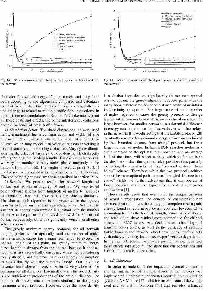
Fig. 10. 30 km network length: Total path energy vs. number of nodes inthe network

simulator focuses on energy-efficient routes, and only findspaths according to the algorithms compared and calculatesthe cost to send data through these links, ignoring collisionsand other costs related to multiple traffic flow interactions. Incontrast, the ns2 simulations in Section IV-C take into accountall these costs and effects, including interference, collisions,and the presence of cross-traffic flows.

1) Simulation Setup: The three-dimensional network usedin the simulations has a constant depth and width (of size400 m and 2 km, respectively) and a length of either 30 or50 km, which may model a network of sensors traversing along distance (e.g., monitoring a pipeline). Varying the dimen-sion has the effect of varying the node density, which directlyaffects the possible per-hop lengths. For each simulation run,we vary the number of relay nodes placed randomly in thenetwork from 1 to 150. The sender is fixed at point (0, 0, 0)and the receiver is placed at the opposite corner of the network.The compared algorithms are those described in section IV-A.

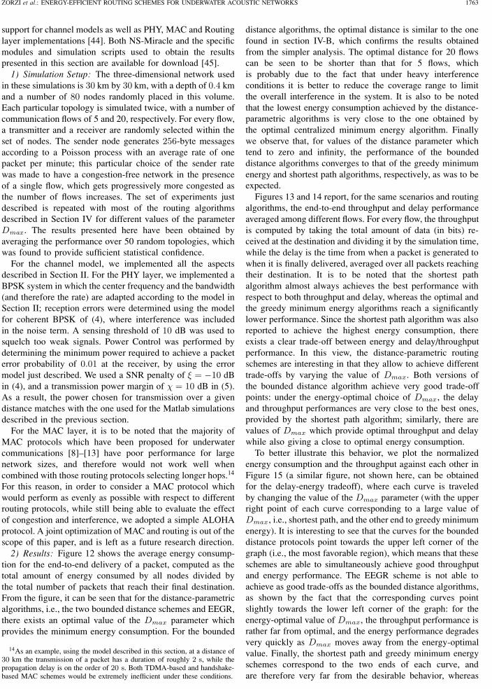
2) Results: We present results for network lengths of30 km and 50 km in Figures 10 and 11. We also testedother network lengths from hundreds of meters to hundredsof kilometers, but omit those results here due to similarity.The shortest path algorithm is not presented in the figures,in order to focus on the most interesting curves. Suffice it tosay that its energy consumption is constant with the numberof nodes and equal to around 8.3 J and 37 J for 30 km and50 km, respectively, which is significantly worse than all otherschemes shown.

The greedy minimum energy protocol, for all networklengths, performs near optimally until the number of nodesin the network causes the average hop length to exceed theoptimal length. At this point, the greedy minimum energycurve begins to diverge from the optimal because it chooseshops that are individually cheapest, while not consideringtotal path cost, and therefore its overall energy consumptionincreases linearly with the number of nodes. Our “boundeddistance from above” protocol performs very close to theoptimum for all distances. Essentially, when the node densityis not sufficient to provide hops of the optimal distance, thebounded distance protocol performs similarly to the greedyminimum energy protocol. However, once the node density

0 10 20 30 40 50 60 70 80

4

5

6

7

8

9

10

Number of nodes in network

Tot

al p

ath

ener

gy [J

]

Greedy min energyBounded distance from belowBounded distance from aboveGeRaFOptimal (Dijkstra)EEGR

Fig. 11. 50 km network length: Total path energy vs. number of nodes inthe network

is such that hops that are significantly shorter than optimalstart to appear, the greedy algorithm chooses paths with toomany hops, whereas the bounded distance protocol maintainsits proximity to optimal. For larger networks, the numberof nodes required to cause the greedy protocol to divergesignificantly from our bounded distance protocol may be quitelarge; however, for smaller networks, a substantial differencein energy consumption can be observed even with few relaysin the network. It is worth noting that the EEGR protocol [28]eventually reaches the minimum energy performance achievedby the “bounded distance from above” protocol, but for alarger number of nodes. In fact, EEGR searches nodes in acircle centered on the optimal relay position, and on averagehalf of the times will select a relay which is farther fromthe destination than the optimal relay position, thus partiallyexhibiting the drawbacks of the “bounded distance frombelow” scheme. Therefore, while the two protocols achievealmost the same optimal performance, “bounded distance fromabove” yields the further advantage that it can operate atlower densities, which are typical for a host of underwaterapplications [1].

These results show that even with the unique behaviorof acoustic propagation, the concept of characteristic hopdistance (that minimizes the energy consumption over a path)already found in radio networks still applies. However, whileaccounting for the effects of path length, transmission distance,and attenuation, these results ignore competition for channelaccess and MAC issues. Any decisions on scheduling andtransmit power levels, as well as the existence of multipletraffic flows in the network, affect how nodes interfere witheach other, which may lead to severe performance degradation.In the next subsection, we provide results that explicitly takethese effects into account, and show that our conclusions stillhold in more realistic scenarios.

C. ns2 Simulator

In order to understand the impact of channel contentionand the interaction of multiple flows in the network, weimplemented a complete underwater acoustic communicationsystem in NS-Miracle [42], which is an extension of the widelyused ns2 simulation platform [43] and provides enhanced



support for channel models as well as PHY, MAC and Routinglayer implementations [44]. Both NS-Miracle and the specificmodules and simulation scripts used to obtain the resultspresented in this section are available for download [45].

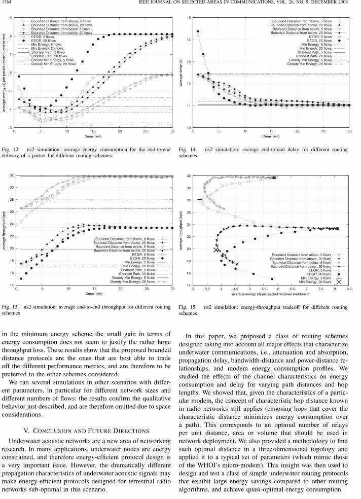
1) Simulation Setup: The three-dimensional network usedin these simulations is 30 km by 30 km, with a depth of 0.4 kmand a number of 80 nodes randomly placed in this volume.Each particular topology is simulated twice, with a number ofcommunication flows of 5 and 20, respectively. For every flow,a transmitter and a receiver are randomly selected within theset of nodes. The sender node generates 256-byte messagesaccording to a Poisson process with an average rate of onepacket per minute; this particular choice of the sender ratewas made to have a congestion-free network in the presenceof a single flow, which gets progressively more congested asthe number of flows increases. The set of experiments justdescribed is repeated with most of the routing algorithmsdescribed in Section IV for different values of the parameterDmax . The results presented here have been obtained byaveraging the performance over 50 random topologies, whichwas found to provide sufficient statistical confidence.

For the channel model, we implemented all the aspectsdescribed in Section II. For the PHY layer, we implemented aBPSK system in which the center frequency and the bandwidth(and therefore the rate) are adapted according to the model inSection II; reception errors were determined using the modelfor coherent BPSK of (4), where interference was includedin the noise term. A sensing threshold of 10 dB was used tosquelch too weak signals. Power Control was performed bydetermining the minimum power required to achieve a packeterror probability of 0.01 at the receiver, by using the errormodel just described. We used a SNR penalty of ξ = −10 dBin (4), and a transmission power margin of χ = 10 dB in (5).As a result, the power chosen for transmission over a givendistance matches with the one used for the Matlab simulationsdescribed in the previous section.

For the MAC layer, it is to be noted that the majority ofMAC protocols which have been proposed for underwatercommunications [8]–[13] have poor performance for largenetwork sizes, and therefore would not work well whencombined with those routing protocols selecting longer hops.14

For this reason, in order to consider a MAC protocol whichwould perform as evenly as possible with respect to differentrouting protocols, while still being able to evaluate the effectof congestion and interference, we adopted a simple ALOHAprotocol. A joint optimization of MAC and routing is out of thescope of this paper, and is left as a future research direction.

2) Results: Figure 12 shows the average energy consump-tion for the end-to-end delivery of a packet, computed as thetotal amount of energy consumed by all nodes divided bythe total number of packets that reach their final destination.From the figure, it can be seen that for the distance-parametricalgorithms, i.e., the two bounded distance schemes and EEGR,there exists an optimal value of the Dmax parameter whichprovides the minimum energy consumption. For the bounded

14As an example, using the model described in this section, at a distance of30 km the transmission of a packet has a duration of roughly 2 s, while thepropagation delay is on the order of 20 s. Both TDMA-based and handshake-based MAC schemes would be extremely inefficient under these conditions.

distance algorithms, the optimal distance is similar to the onefound in section IV-B, which confirms the results obtainedfrom the simpler analysis. The optimal distance for 20 flowscan be seen to be shorter than that for 5 flows, whichis probably due to the fact that under heavy interferenceconditions it is better to reduce the coverage range to limitthe overall interference in the system. It is also to be notedthat the lowest energy consumption achieved by the distance-parametric algorithms is very close to the one obtained bythe optimal centralized minimum energy algorithm. Finallywe observe that, for values of the distance parameter whichtend to zero and infinity, the performance of the boundeddistance algorithms converges to that of the greedy minimumenergy and shortest path algorithms, respectively, as was to beexpected.

Figures 13 and 14 report, for the same scenarios and routingalgorithms, the end-to-end throughput and delay performanceaveraged among different flows. For every flow, the throughputis computed by taking the total amount of data (in bits) re-ceived at the destination and dividing it by the simulation time,while the delay is the time from when a packet is generated towhen it is finally delivered, averaged over all packets reachingtheir destination. It is to be noted that the shortest pathalgorithm almost always achieves the best performance withrespect to both throughput and delay, whereas the optimal andthe greedy minimum energy algorithms reach a significantlylower performance. Since the shortest path algorithm was alsoreported to achieve the highest energy consumption, thereexists a clear trade-off between energy and delay/throughputperformance. In this view, the distance-parametric routingschemes are interesting in that they allow to achieve differenttrade-offs by varying the value of Dmax. Both versions ofthe bounded distance algorithm achieve very good trade-offpoints: under the energy-optimal choice of Dmax, the delayand throughput performances are very close to the best ones,provided by the shortest path algorithm; similarly, there arevalues of Dmax which provide optimal throughput and delaywhile also giving a close to optimal energy consumption.

To better illustrate this behavior, we plot the normalizedenergy consumption and the throughput against each other inFigure 15 (a similar figure, not shown here, can be obtainedfor the delay-energy tradeoff), where each curve is traveledby changing the value of the Dmax parameter (with the upperright point of each curve corresponding to a large value ofDmax, i.e., shortest path, and the other end to greedy minimumenergy). It is interesting to see that the curves for the boundeddistance protocols point towards the upper left corner of thegraph (i.e., the most favorable region), which means that theseschemes are able to simultaneously achieve good throughputand energy performance. The EEGR scheme is not able toachieve as good trade-offs as the bounded distance algorithms,as shown by the fact that the corresponding curves pointslightly towards the lower left corner of the graph: for theenergy-optimal value of Dmax, the throughput performance israther far from optimal, and the energy performance degradesvery quickly as Dmax moves away from the energy-optimalvalue. Finally, the shortest path and greedy minimum energyschemes correspond to the two ends of each curve, andare therefore very far from the desirable behavior, whereas



3

4

5

6

7

8

9

0 5 10 15 20 25 30

aver

age

ener

gy (

J) p

er p

acke

t rec

eive

d en

d-to

-end

Dmax (km)

Bounded Distance from above, 5 flowsBounded Distance from above, 20 flowsBounded Distance from below, 5 flowsBounded Distance from below, 20 flowsEEGR, 5 flowsEEGR, 20 flowsMin Energy, 5 flowsMin Energy, 20 flowsShortest Path, 5 flowsShortest Path, 20 flowsGreedy Min Energy, 5 flowsGreedy Min Energy, 20 flows

Fig. 12. ns2 simulation: average energy consumption for the end-to-enddelivery of a packet for different routing schemes

14

16

18

20

22

24

26

28

30

32

0 5 10 15 20 25 30

aver

age

thro

ughp

ut (

bps)

Dmax (km)

Bounded Distance from above, 5 flowsBounded Distance from above, 20 flows

Bounded Distance from below, 5 flowsBounded Distance from below, 20 flows

EEGR, 5 flowsEEGR, 20 flows

Min Energy, 5 flowsMin Energy, 20 flows

Shortest Path, 5 flowsShortest Path, 20 flows

Greedy Min Energy, 5 flowsGreedy Min Energy, 20 flows

Fig. 13. ns2 simulation: average end-to-end throughput for different routingschemes

in the minimum energy scheme the small gain in terms ofenergy consumption does not seem to justify the rather largethroughput loss. These results show that the proposed boundeddistance protocols are the ones that are best able to tradeoff the different performance metrics, and are therefore to bepreferred to the other schemes considered.

We ran several simulations in other scenarios with differ-ent parameters, in particular for different network sizes anddifferent numbers of flows: the results confirm the qualitativebehavior just described, and are therefore omitted due to spaceconsiderations.

V. CONCLUSION AND FUTURE DIRECTIONS

Underwater acoustic networks are a new area of networkingresearch. In many applications, underwater nodes are energyconstrained, and therefore energy-efficient protocol design isa very important issue. However, the dramatically differentpropagation characteristics of underwater acoustic signals maymake energy-efficient protocols designed for terrestrial radionetworks sub-optimal in this scenario.

10

11

12

13

14

15

0 5 10 15 20 25 30

aver

age

dela

y (s

)

Dmax (km)





Shortest Path, 5 flowsShortest Path, 20 flows

Greedy Min Energy, 5 flowsGreedy Min Energy, 20 flows

Fig. 14. ns2 simulation: average end-to-end delay for different routingschemes

14

16

18

20

22

24

26

28

30

32

3 3.5 4 4.5 5 5.5 6 6.5 7 7.5 8 8.5

aver

age

thro

ughp

ut (

bps)

average energy (J) per packet received end-to-end





Fig. 15. ns2 simulation: energy-throughput tradeoff for different routingschemes

In this paper, we proposed a class of routing schemesdesigned taking into account all major effects that characterizeunderwater communications, i.e., attenuation and absorption,propagation delay, bandwidth-distance and power-distance re-lationships, and modem energy consumption profiles. Westudied the effects of the channel characteristics on energyconsumption and delay for varying path distances and hoplengths. We showed that, given the characteristics of a partic-ular modem, the concept of characteristic hop distance knownin radio networks still applies (choosing hops that cover thecharacteristic distance minimizes energy consumption overa path). This corresponds to an optimal number of relaysper unit distance, area or volume that should be used innetwork deployment. We also provided a methodology to findsuch optimal distance in a three-dimensional topology andapplied it to a typical set of parameters (which mimic thoseof the WHOI’s micro-modem). This insight was then used todesign and test a class of simple underwater routing protocolsthat exhibit large energy savings compared to other routingalgorithms, and achieve quasi-optimal energy consumption.



Finally, to validate our results for realistic network sce-narios, we designed routing protocols based on the analysisand showed that our solution outperforms strategies that arecommonly considered in terrestrial wireless sensor networks.Performance evaluation was carried out first in Matlab usinga detailed model of the underwater acoustic channel, and sub-sequently in ns2 to be able to characterize, in addition to thechannel, important aspects of the PHY and MAC componentsof an underwater communication system. Both evaluationmethods confirmed that the proposed routing strategy achievesa higher energy efficiency compared to other schemes, and isactually close to the optimal energy performance, while at thesame time achieving a very good trade-off with respect tothroughput and delay.

Future research includes further optimizations and param-eter tuning of the protocol, integrating this work with idle-time power management, and consideration of other MAClayer protocols. Also, extending the link capacity analysisto a network capacity analysis (by explicitly including theinterference) could lead to further observations that wouldimpact the design of protocols at all layers of the networkstack.

REFERENCES

[1] I. Akyildiz, D. Pompili, and T. Melodia, “Underwater acoustic sensornetworks: Research challenges,” Elsevier Ad Hoc Networks, vol. 3, no. 3,pp. 257–279, 2005.

[2] J. Heidemann, W. Ye, J. Willis, A. Syed, and Y. Li, “Research challengesand applications for underwater sensor networking,” in Proc. IEEEWireless Communications of Networking Conference (WCNC), LasVegas, USA, Apr 2006.

[3] E. M. Sozer, M. Stojanovic, and J. G. Proakis, “Underwater acousticnetworks,” IEEE J. Oceanic Eng., vol. 25, no. 1, pp. 72–83, Jan. 2000.

[4] H. Song, W. Hodgkiss, and W. Kuperman, “MIMO Time ReversalCommunications,” in Proc. International Workshop on UnderWaterNetworks (WUWNet), Montreal, Canada, Sep 2007.

[5] S. Hwang and P. Schniter, “Efficient multicarrier communication forhighly spread underwater acoustic channels,” IEEE J. Select. AreasCommun., this issue, 2008.

[6] D. Lucani, M. Medard, and M. Stojanovic, “Network coding schemesfor underwater networks: The benefits of implicit acknowledgement,”in Proc. International Workshop on UnderWater Networks (WUWNet),Montreal, Canada, Sep 2007.

[7] L. Freitag, M. Grund, S. Singh, J. Partan, and P. K. K. Ball, “The WHOImicro-modem: an acoustic communications and navigation system formultiple platforms,” in Proc. MTS/IEEE Conference and Exhibition forOcean Engineering, Science and Technology (OCEANS), Washington,DC, USA, Sep 2005.

[8] M. Molins and M. Stojanovic, “Slotted FAMA: a MAC protocol forunderwater acoustic networks,” in Proc. MTS/IEEE Conference andExhibition for Ocean Engineering, Science and Technology (OCEANS),Raffles City, Singapore, May 2006.

[9] B. Peleato and M. Stojanovic, “A MAC protocol for ad hoc underwateracoustic sensor networks,” in Proc. International Workshop on Under-Water Networks (WUWNet), Los Angeles, CA, USA, Sep 2006.

[10] V. Rodoplu and M. Park, “An energy-efficient MAC protocol for under-water wireless acoustic networks,” in Proc. MTS/IEEE Conference andExhibition for Ocean Engineering, Science and Technology (OCEANS),Brest, France, Jun 2005.

[11] A. Syed, W. Ye, and J. Heidemann, “Comparison and Analysis of T-Lohi MAC for Underwater Acoustic Sensor Networks,” IEEE J. Select.Areas Commun., this issue, 2008.

[12] A. Syed, W. Ye, B. Krishnamachari, and J. Heidemann, “Understandingspatio-temporal uncertainty in medium access with aloha protocols,”in Proc. International Workshop on UnderWater Networks (WUWNet),Montreal, Canada, Sep 2007.

[13] K. B. Kredo and P. Mohapatra, “A hybrid medium access controlprotocol for underwater wireless networks,” in Proc. InternationalWorkshop on UnderWater Networks (WUWNet), Montreal, Canada, Sep2007.

[14] D. Pompili, T. Melodia, and I. F. Akyildiz, “A distributed CDMAmedium access control for underwater acoustic sensor networks,” inProc. IFIP Annual Mediterranean Ad Hoc Networking Workshop (Med-Hoc-Net), Corfu, Greece, Jun. 2007.

[15] E. Sozer, M. Stojanovic, and J. Proakis, “Initialization and routingoptimization for ad hoc underwater acoustic networks,” in Proc. OP-NETWORK, Washington, DC, Sep. 2000.

[16] R. Nitzel, C. Benton, S. G. Chappell, and D. R. Blidberg, “Exploitingdynamic source routing to enable undersea networking over an ad-hoctopology,” in Proc. International Symposium on Underwater Technology,Tokyo, Japan, Apr. 2002.

[17] D. Pompili, T. Melodia, and I. Akyildiz, “Routing algorithms for delay-insensitive and delay-sensitive applications in underwater sensor net-works,” in Proc. Annual International Conference on Mobile Computingand Networking (MobiCom), Los Angeles, CA, USA, Sep 2006.

[18] ——, “A resilient routing algorithm for long-term applications inunderwater sensor networks,” in Proc. IFIP Annual Mediterranean AdHoc Networking Workshop (Med-Hoc-Net), 2006.

[19] M. Zorzi and R. R. Rao, “Geographic Random Forwarding (GeRaF) forAd Hoc and Sensor Networks: Energy and Latency Performance,” IEEETrans. Mobile Comput., vol. 2, no. 4, pp. 349–365, 2003.

[20] K. Kar, M. Kodialam, T. V. Lakshman, and L. Tassiulas, “Routing fornetwork capacity maximization in energy-constrained ad-hoc networks,”in Proc. of the IEEE Conference on Computer Communications (INFO-COM), San Francisco, CA, USA, Apr 2003.

[21] J.-H. Chang and L. Tassiulas, “Energy conserving routing in wireless ad-hoc networks,” in Proc. IEEE Conference on Computer Communications(INFOCOM), Tel-Aviv, Israel, Mar 2000.

[22] S. Banerjee and A. Misra, “Minimum energy paths for reliable commu-nication in multi-hop wireless networks,” in Proc. ACM InternationalSymposium on Mobile Ad Hoc Networking and Computing (MobiHoc),Lausanne, Switzerland, Jun 2002.

[23] Y. Xu, J. Heidemann, and D. Estrin, “Geography-informed energy con-servation for ad hoc routing,” in Proc. Annual International Conferenceon Mobile Computing and Networking (MobiCom), Rome, Italy, Jul2001.

[24] R. C. Shah and J. M. Rabaey, “Energy aware routing for low energyad hoc sensor networks,” in Proc. IEEE Wireless Communications ofNetworking Conference (WCNC), Orlando, FL, USA, Mar 2002.

[25] C. Sengul and R. Kravets, “Conserving energy with on-demand topologymanagement,” in Proc. IEEE International Conference on Mobile AdHoc and Sensor Systems (MASS), Washington, DC, USA, Nov 2005.

[26] M. Bhardwaj, T. Garnett, and A. P. Chandrakasan, “Upper bounds on thelifetime of sensor networks,” in Proc. IEEE International Conference onCommunications (ICC), Helsinki, Finland, Jun 2001.

[27] J. Wang and I. Howitt, “Optimal traffic distribution in minimum energywireless sensor networks,” in Proc. IEEE Global CommunicationsConference (GLOBECOM), St. Louis, MO, USA, Nov-Dec 2005.

[28] H. Zhang and H. Shen, “EEGR: energy-efficient geographic routing inwireless sensor networks,” in Proc. of the IEEE International ConferenceOn Parallel Processing (ICPP), Xian, China, Sep 2007.

[29] P. Gupta and P. R. Kumar, “The capacity of wireless networks,” IEEETrans. Inform. Theory, vol. 46, no. 2, pp. 388–404, Mar 2000.

[30] M. Stojanovic, “On the relationship between capacity and distance inan underwater acoustic communication channel,” in Proc. of the Inter-national Workshop on UnderWater Networks (WUWNet), Los Angeles,CA, USA, Sep 2006.

[31] R. Urick, Principles of Underwater Sound. McGraw-Hill, 1983.[32] L. Berkhovskikh and Y. Lysanov, Fundamentals of Ocean Acoustics.

Springer, 1982.[33] A. Goldsmith, Wireless Communications. Cambridge University Press,

2005.[34] Aironet, “PC4800 user guide,” 1998, http://www.aironet.com/.[35] A. F. Harris III, M. Stojanovic and M. Zorzi, “When underwater acoustic

nodes should sleep with one eye open: idle–time power managementin underwater sensor networks,” in Proc. International Workshop onUnderWater Networks (WUWNet), Los Angeles, CA, Sep. 2006, pp.105–108.

[36] D. Mirza and C. Schurgers, “Energy-efficient localization in networksof underwater drifters,” in Proc. International Workshop on UnderWaterNetworks (WUWNet), Montreal, Canada, Sep 2007.

[37] M. Erol, L. Vieira, and M. Gerla, “Localization with Dive’N’Rise (DNR)Beacons for Underwater Acoustic Sensor Networks,” in Proc. of theInternational Workshop on UnderWater Networks (WUWNet), Montreal,Canada, Sep 2007.

[38] D. Mirza and C. Schurgers, “Energy-efficient ranging for post-factoself-localization in mobile underwater networks,” IEEE J. Select. AreasCommun., this issue, 2008.



[39] P. Casari, M. Nati, C. Petrioli, and M. Zorzi, “Efficient non–planarrouting around dead ends in sparse topologies using random forward-ing,” in Proc. IEEE International Conference on Communications (ICC),Glasgow, Scotland, Jun 2007.

[40] B. Karp and H. T. Kung, “GPSR: greedy perimeter stateless routing forwireless sensor networks,” Proc. Annual International Conference onMobile Computing and Networking (MobiCom), Aug 2000.

[41] J. M. J. Montana, M. Stojanovic, and M. Zorzi, “Focused beam routingprotocol for underwater acoustic networks,” in Proc. InternationalWorkshop on UnderWater Networks (WUWNet), San Francisco, CA,Sep. 2008.

[42] N. Baldo, F. Maguolo, M. Miozzo, M. Rossi, and M. Zorzi, “NS2-MIRACLE: a Modular Framework for Multi-Technology and Cross-Layer Support in Network Simulator 2,” in Proc. ACM InternationalWorkshop on Network Simulation Tools (NSTOOLS), Nantes, France,Oct 2007.

[43] ns2 Network Simulator, http://www.isi.edu/nsnam/ns/.[44] N. Baldo, F. Maguolo, and M. Miozzo, “A new approach to simulating

PHY, MAC and Routing,” in Proc. ACM International Workshop onNS-2, Athens, Greece, Oct 2008.

[45] “Model for underwater channel in ns2,” 2008. [Online]. Available:http://telecom.dei.unipd.it/download/

Michele Zorzi (S’89, M’95, SM’98, F’07) wasborn in Venice, Italy, in 1966. He received theLaurea degree and the Ph.D. degree in ElectricalEngineering from the University of Padova, Italy, in1990 and 1994, respectively. During the AcademicYear 1992/93, he was on leave at the University ofCalifornia, San Diego (UCSD), attending graduatecourses and doing research on multiple access inmobile radio networks. In 1993, he joined the facultyof the Dipartimento di Elettronica e Informazione,Politecnico di Milano, Italy. After spending three

years with the Center for Wireless Communications at UCSD, in 1998 hejoined the School of Engineering of the University of Ferrara, Italy, and in2003 joined the Department of Information Engineering of the University ofPadova, Italy, where he is currently a Professor. His present research interestsinclude performance evaluation in mobile communications systems, randomaccess in mobile radio networks, ad hoc and sensor networks, and energyconstrained communications protocols.

Dr. Zorzi was the Editor-In-Chief of the IEEE WIRELESS COMMUNICA-TIONS MAGAZINE from 2003 to 2005, is currently the Editor-In-Chief of theIEEE TRANSACTIONS ON COMMUNICATIONS, and serves on the SteeringCommittee of the IEEE TRANSACTIONS ON MOBILE COMPUTING, and onthe Editorial Boards of the IEEE TRANSACTIONS ON COMMUNICATIONS,the IEEE TRANSACTIONS ON WIRELESS COMMUNICATIONS, the WILEYJOURNAL OF WIRELESS COMMUNICATIONS AND MOBILE COMPUTING andthe ACM/URSI/KLUWER JOURNAL OF WIRELESS NETWORKS. He wasalso guest editor for special issues in the IEEE PERSONAL COMMUNICA-TIONS MAGAZINE (Energy Management in Personal Communications Sys-tems) and the IEEE JOURNAL ON SELECTED AREAS IN COMMUNICATIONS

(Multi-media Network Radios).

Paolo Casari (S’05-M’08) was born in Ferrara,Italy, on August 20th, 1980. He received the Laureadegree (BE) in Electronics and TelecommunicationsEngineering (2002) and the Laurea Specialisticadegree (ME) in Telecommunications Engineering(2004) summa cum laude, both from the Universityof Ferrara, and the Ph.D. degree in InformationEngineering (2008) from the University of Padova.In 2007 he was on leave at the MassachusettsInstitute of Technology, Cambridge, MA, workingon energyefficient protocol design for underwater

acoustic sensor networks. He currently holds a post doctorate research positionat the University of Padova. His main research interest is crosslayer protocoldesign for wireless networks through PHY/MAC/routing interactions, with aparticular focus on MIMO ad hoc networks, wireless sensor networks, andunderwater acoustic networks.

Nicola Baldo (S’07) was born in Rovigo, Italy,in 1981. He received his Laurea (BE) and LaureaSpecialistica (ME) degree in TelecommunicationsEngineering in 2003 and 2005, respectively, fromthe University of Ferrara, Italy. In summer 2003he was an internship student at the Ericsson Eu-rolab Deutschland, Aachen, Germany, working onWireless Multimedia Communications. In 2005 hewas on leave at the STMicroelectronics AdvancedSystem Technology group, Agrate Brianza (MI),Italy, working on Cross-layer Optimization for VoIP

over Wireless LAN. Since 2006 he is a Ph.D. student at the University ofPadova, Italy, under supervision by Prof. Michele Zorzi. In 2008 he was onleave at the Calit2 department, University of California, San Diego, workingon Cognitive Networks and Software Defined Radio. His research interestsinclude Cognitive Radio and Networks, Cross-layer Optimization, UnderwaterCommunications and Network Simulation Tools.

Albert F. Harris III is a research assistant professorat the University of Kansas in the Center for RemoteSensing of Ice Sheets (CReSIS). He earned his Ph.D.in computer science from the University of Illinoisat Urbana-Champaign, specializing in wireless net-work protocol and mobile systems design. Followinghis time at UIUC, he completed a one year post doc-torate position at the University of Padova, Italy. Hiscurrent interests are underwater acoustic networks,delay tolerant networks, and network support forassisted living and disaster recovery environments.


energy-efficient routing schemes for underwater acoustic networks

Documents