enen4001 – l3 – filtration
TRANSCRIPT

ENEN4001 – L3 – Filtration The answers provided for the following questions offer some identification and scope of the solution
areas. They are by no means fully comprehensive, and could be improved upon and added to should
you want to take any section in further depth. However, the answers suggested are typical of those
provided by a student achieving a high distinction. You may find, in some cases, that you have used
valid reasoning and appropriate facts and concluded an alternative recommendation to the one
provided – which is acceptable. In some cases, additional text has been provided for you to
understand in greater depth the issues within the question. This is denoted by an italicised font.
Section 1 – Rapid Filter Theories & Behaviours 1. Although mechanical straining is often considered to be the only removal method for flow
through granular filters, this method only accounts for a small proportion of the suspended
solids removed from the fluid.
The mechanical properties of the filer cause particle removal through straining (as 1) where
the particles are too large to fit through a gap between solids. Particle 2 represents
sedimentation, where a suspended solid deviates from the streamline sufficiently to settle on
a filter grain.
The adsoprtion methods of the filter include flocculation (as 3), where small particles are
attracted to larger flocs that are already attached to the surface of the granular medium. This
requires particles to be adhered to the filter particle, and hence explains the lack of efficiency
of a new (clean) filter, and the subsequent ripening phase. Particle 4 demonstrates
interception, where a particle maintains its place in a streamline, but is large enough to collide
and become attached to the filter particle. The final method, diffusion (no 5) involves the
Brownian motion of a particle, moving against a streamline to become attached to a filter
particle.
2. Clean bed filtration is the filtering process applied when a bed of cleaned filter medium is
used. Over time, due to the filtration process, the solids are deposited within the voids, which
decreases the porosity, therefore requires a faster void velocity of the fluid, which
subsequently increases head losses. The head loss over time should be monitored to give an
indication of the sediment deposition depth within the filter – as filters typically gather
deposition in the voids of highest elevation. Headloss is approximately correlated to
deposited solids, and therefore monitoring headloss can give a clear indication of the
performance of the filter and its place in the filter/wash cycle.
5
1
2
3
4
5

3. In order for a particle to function as a filter material, it needs the suspended solid to contact
against the particle, and also to then become attached to the surface. These are two separate
mechanisms, with different causes and requirements.
𝛼 is the measure of efficiency of the contact of a filter particle, and is defined as the ratio of
the number of contacting particles to the number of particles approaching the grain. This is a
physical parameter, and takes into account the physical properties of the grain, e.g. the
sphericity, porosity, etc.
𝜂 is a measure of the attachment efficiency, and is defined as the ratio of number of adhering
of the particles to the number of contacting particles. This is a measure of the chemical
attraction of the particles to the physical media, and will particularly on the DLVO theory of
double diffuse layer – i.e. how much chemical attraction there can be between particles, given
the Van Der Waals forces, etc.
Combining these measures, 𝜂 × 𝛼 gives a total measure of efficiency of the media.
4. When considering collector efficiency to suspended (removable) particle size, the larger the
diameter of the particle, the more important the mechanical removal methods are – i.e. the
larger particles will be strained effectively and sediment easily. The smaller particles will be
able to move more significantly under Brownian motion – allowing more diffusion and,
assuming a small enough porosity, this significantly increases the probability of removal. The
balancing point between these two methods, typically falls around 1𝜇𝑚.
5. If we consider the removal percentage with depth – remembering that typically stratified
filters have smaller particles at the top and larger at the bottom.
The black line shown gives the typical response of a filter medium – a significant decrease in
the upper layers of the filters caused by the finer particles removing a significant proportion
of the material, but lower depths maintaining capability of removing particles. If we increase
the uniformity coefficient, we are increasing the spread of the particle sizes (𝑈 = 𝑑60/𝑑10),
and therefore the change in particle sizes over depth will increase, leaving a thinner layer of
smaller particles (and more effective filtration), and larger layer of particles with bigger voids,
and less effective filtration. This tends to look like the blue dashed line shown above –
maintaining a similar to slightly improved removal rate in the upper layers (assuming similar
values of 𝐸), but a rapidly dropping efficiency as the particles get bigger and less effective at
removing suspended solids.
Depth
Filtrate particle
counts

6. In-depth filtration refers to the concept of removing suspended solids throughout the filter
medium – i.e., ensuring non-trivial removal rates at all depths within the media. The key
factors that encourage this are to ensure a filter media that has a low coefficient of uniformity
– i.e. the media maintains a similar size. In addition to this, using a dual-media filter will
significantly improve the filtration in depth (provided the larger media settles on the top of
the filter, typically ensured by using a lighter material, e.g. anthracite over sand, sand over
garnet, etc). Ensuring in-depth filtration typically means that the filter bed can be shallower,
offering the same removal rates, and will typically have longer between backwashing due to
the larger void volumes to store suspended solids.
7. Backwashing is a process whereby clean water is pumped through the granular filter in the
reverse direction to the normal filtration method. Normally, this means backwashing involves
pumping vertically upwards. The mobilised filter particles are fluidised, and in the process
move laterally and collide with each other. As a result of this, the lighter, often flocculated,
contaminants are stripped from the filter media through a combination of collision and drag
caused by the fluid velocity. These contaminates are subsequently brought to the surface and
washed into troughs.
After backwashing, the cleaned filter media is allowed to settle, and water resumes normal
flow. During the initial stage of filtering, the effluent is a higher turbidity than normal, as the
presence of contaminants increases the filter performance (through decreasing void space
and increasing flocculation). That contaminants initiate an improvement in filtration means
that the initial flow has a higher turbidity, and although the average turbidity level is low
enough to warrant the initial water inclusion, the potential for breakthrough of disease
(particularly giardia and cryptosporidium – both highly resistant to disinfectants) requires the
water to be wasted, or carefully recycled.
8.
1) Sand boiling occurs during the backwash of a filter. Instead of the water expanding
the bed evenly, a significant proportion of the water appears to be converging to a
particular point on the surface, as seen in the diagram below. Typically, this is caused
by a slight weakness in the soil bed that subsequently erodes in (similar to a piping
mechanism). Invariably this will cause a failure in the filter due to fines washing out,
in addition to an uneven expansion of the bed. It can be caused by ruptures in the
underdrain, or weakness in the filter bed. The filter is likely to be required to be re-
laid.
.
2) Mud balls occur during backwash – if there is a significant enough conglomeration of
particles that the mass is high enough to avoid wash-out, the ball can grow using
adsorption in both backwash and normal use. At the end of backwash, the mud balls
typically fall to the bottom of the filter, where they can pollute the effluent.
Water Level
Filter Media
Underdrain

9. The nature of a dual media filter means that a larger void space is contained in the upper
media, offering a significant space for larger suspended sediment to be removed. The lower
layer and its smaller void space results in the smaller suspended sediment to be removed
without clogging. This means that the filter can have longer filter runs before a inducing a
large headloss.
However, dual media designs require careful sourcing and design of the filter material. The
settling velocities of the larger material must be lower than the smaller material in order to
maintain segregation. In addition, the backwash velocities are more constricted. Coagulation
and Flocculation is also necessary for dual media filters. Note that it is almost always used for
single media filtration, but is not required unless higher (>1ms-1) flow rates are required.
10. Constant Flow – Constant Head
The filters are maintained with a constant water level above the filter. Initially, the outlet
valve is partially closed and flow through the filter is set to a pre-determined rate. As the
headloss builds up in the filter, the effluent valve is opened further to maintain the flow.
When the valve is fully open and the flow drops, the backwashing cycle begins.
Constant Flow – Variable Head
Initially the filters are submerged beneath a small water value, and as the headloss builds in
the filter, the water head above the filter is increased to maintain a constant flow. When the
water head reaches a predetermined level, the backwashing cycle begins.
Variable Flow – Constant Head
Water is split over the filters and the flow through individual filters reduces as headloss
increases. When a particular filter is backwashed, there will be a slight increase in head above
the filters, but generally the water level is maintained by having a constant average headloss
over the filters, and rotating the backwashing cycles.

Section 2 – Filter Material 11.
1) Sand Source 1 appears to be a naturally occurring sand – as noted by the distinct
curves in the soil particle distribution plot:
This sand has an effective size of 𝐸 = 𝑑10 = 0.53𝑚𝑚, and a Coefficient of Uniformity
of 𝑈 =𝑑60
𝑑10= 1.55. Comparing to the appropriate guidelines, it is clear this does fall
in the material properties values – however, the large upper tail may result in difficulty
designing the backwash.
2) This material offers a good profile, as it is more linear than the sample in A, however
the particles are too big, giving values of 𝐸 = 0.99𝑚. The uniformity coefficient is
acceptable, given 𝑈 = 1.53. There is no processing that can reduce the sand size, as
there is insufficient smaller media.

3) This sample offers a good uniform grading, with 𝑈 = 1.55. The effective size of the
media is 𝐸 = 0.37𝑚𝑚, which is slightly below the recommended guidelines, but may
be considered acceptable. If this is not the case, then the lowest fines could be driven
off in situ during a preliminary backwash.
12. Considering the values given, the filter material is shown by the following plot:
This gives values of 𝐸 = 0.42𝑚𝑚 and 𝑈 = 1.408, which fall within the guidelines. Calculating
the settling velocities:
𝑑𝑚𝑖𝑛 = 0.297𝑚𝑚
𝑉𝑔𝑢𝑒𝑠𝑠~𝑑2𝑔(𝜌𝑠 − 𝜌𝑤)
18𝜇= 0.07𝑚𝑠−1
𝑅𝑒 =𝜓𝑉𝑠𝐷
𝜈= 14.87
𝐶𝐷 =24
𝑅𝑒+
3
√𝑅𝑒+ 0.34 = 2.73
𝑉𝑆 = √4𝑔𝑑(𝜌𝑠 − 𝜌𝑤)
3𝜌𝑤𝐶𝐷= 0.0485𝑚𝑠−1
And iterating through…
𝑉𝑠 = 0.0387𝑚𝑠−1
If we considered 𝑑10, we would get:

𝑉𝑠 = 0.0638
Considering 𝑑90, which has a diameter of 0.83𝑚𝑚, we can calculate:
𝐺𝑎 =𝑑3𝜌𝑤𝑔(𝜌𝑠 − 𝜌𝑤)
𝜇2=
(0.83 × 10⁻³)3 × 999.103 × 9.81 × (2650 − 999.103)
(1.139 × 10⁻³)2
𝐺𝑎 = 7132
Hence:
𝑉𝐹 = 1.3𝑣
𝑑(√33.72 + 0.0408𝐺𝑎 − 33.7)
𝑉𝐹 = 1.31.140 × 10−6
0.83 × 10⁻³(√33.72 + 0.0408 × 7132 − 33.7)
𝑉𝐹 = 0.0073𝑚𝑠−1
So any backwash velocity within the limits 0.0073 < 𝑉𝑏 < 0.0387 will fluidise the bed without
washing away any fines.
13. Considering each material in turn, we can see that for sand:
This gives a 𝐸 = 0.44𝑚𝑚, and a 𝑈 = 1.59, which both fit well within the recommended
values.
The Anthracite is a much wider grading, as seen in the graph below:

In this case, we have a value of 𝐸 = 0.38𝑚𝑚 and 𝑈 = 1.84. The effective size is fine, though
the uniformity coefficient is at the upper limit for a dual media filter.
Considering the calculations required:
The backwash value required must be lower than the smallest settling velocity. In this case,
we can consider the settling velocities for both materials:
𝑑10(𝑠𝑎𝑛𝑑) = 0.44𝑚𝑚
𝑉𝑠 = 0.066𝑚𝑠−1
𝑑10(𝑎𝑛𝑡ℎ𝑟𝑎𝑐𝑖𝑡𝑒) = 0.38𝑚𝑚
𝑉𝑠 = 0.047𝑚𝑠−1
Note that it would be an extremely poor filter design for the sand to have a lower settling
velocity than the anthracite, as we would end up with sand overlying anthracite. Indeed, the
later part of the question requires us to check the segregation such that all the anthracite
settles slower than all the sand. However, both are placed here for illumination. Hence, the
backwash velocity must fall below 0.025𝑚𝑠−1
Considering the largest particles of both media:
𝑑90(𝑠𝑎𝑛𝑑) = 1.01𝑚𝑚
𝐺𝑎 =𝑑3𝜌𝑤𝑔(𝜌𝑠 − 𝜌𝑤)
𝜇2=
(1.01 × 10⁻³)3 × 998.599 × 9.81 × (2650 − 998.599)
(1.053 × 10⁻³)2
𝐺𝑎 = 15.03 × 10³
Hence:
𝑉𝐹 = 1.3𝑣
𝑑(√33.72 + 0.0408𝐺𝑎 − 33.7)
𝑉𝐹 = 1.31.054 × 10−6
1.01 × 10⁻³(√33.72 + 0.0408 × 15.03 × 103 − 33.7)
𝑉𝐹 = 0.011𝑚𝑠−1
And for Anthracite:
𝑑90(𝑎𝑛𝑡ℎ𝑟𝑎𝑐𝑖𝑡𝑒) = 1.26𝑚𝑚
𝐺𝑎 =𝑑3𝜌𝑤𝑔(𝜌𝑠 − 𝜌𝑤)
𝜇2=
(1.26 × 10⁻³)3 × 998.599 × 9.81 × (1620 − 998.599)
(1.053 × 10⁻³)2
𝐺𝑎 = 10.98 × 10³
Hence:
𝑉𝐹 = 1.3𝑣
𝑑(√33.72 + 0.0408𝐺𝑎 − 33.7)
𝑉𝐹 = 1.31.054 × 10−6
1.26 × 10⁻³(√33.72 + 0.0408 × 10.98 × 103 − 33.7)
𝑉𝐹 = 0.0067𝑚𝑠−1
Also, for the Anthracite:
𝑉𝑠𝑒𝑡𝑡𝑙𝑖𝑛𝑔(𝑑90) = 0.185𝑚𝑠−1
Hence we can conclude, that with a backwash rate of around 0.04𝑚𝑠−1 we would fluidise the
entire bed (0.04 > 𝑉𝐹(𝑠𝑎𝑛𝑑) > 𝑉𝐹(𝑎𝑛𝑡ℎ𝑟𝑎𝑐𝑖𝑡𝑒). However, the settling velocity of the largest
anthracite particles is much greater than the smallest sand grains, which means that there will
be intermingling of the sand and anthracite after a backwash, and the filter will not function
as intended – as the finest sand will intermingle with the anthracite, which is much more

angular and will result in a high porosity and subsequently a higher turbidity in the effluent
(though a longer filter run).
Indeed, the fast settling of the larger anthracite particles was hinted at as a potential problem
when we considered the uniformity coefficient of the anthracite, and noted its large value.

Section 3 – Filter Design
14. If we use the empirical formula provided, we can see:
𝑁 ≥ 0.0195√𝑄
𝑁 ≥ 0.0195 × √3500 = 1.154
3500𝑚3𝑑𝑎𝑦−1 gives a value of 0.041𝑚3𝑠−1, so two filters is satisfactory (𝑄 < 0.1𝑚3𝑠−1).
Hence, by considering the area required when one is taken offline, we need to be able to
process the total water demand through a single filter:
𝐴 =𝑄
𝑉𝐴=
3500
120= 29.17𝑚2
So we can suggest 3𝑚 × 10𝑚 as a plan area (𝐿: 𝑊 = 3.3: 1).
15. Analysing the filter material:
Giving 𝐸 = 0.33𝑚𝑚 and 𝑈 = 1.68.
Considering the Rose equation:
𝐻𝐿
𝐷=
1.067𝑉𝐹2
𝜓𝑔𝜖4∑
𝐶𝐷𝑓
𝑑
We can calculate the Cd value for each average sieve size:
Size 𝒇 �̅� = √𝑑1𝑑2 𝑹𝒆 =
𝜓𝑉�̅�
𝜈
𝑪𝑫 𝑪𝑫𝒇
𝒅
8-12 0.0001 2.00 2.16 13.49 0.675 12-16 0.0039 1.41 1.52 18.56 51.3 16-20 0.0570 1.00 1.08 25.45 1451 20-30 0.2590 0.707 0.763 35.23 12900 30-40 0.4400 0.500 0.540 48.87 43000 40-50 0.2020 0.353 0.381 68.19 39000 50-70 0.0370 0.250 0.270 95.00 14100 70-100 0.0010 0.177 0.191 132.9 751 SUM 111254

Hence:
𝐻𝐿
𝐷=
1.067
0.8 × 9.81 × 0.424× (
120
24 × 602)
2
× 111254 = 0.938
𝐻𝐿 = 0.938 × 0.6 = 0.56𝑚
And using the Blake-Kozeny equation:
𝐻𝐿
𝐷=
36𝑘𝑧𝜇(1 − 𝜖)2
𝜌𝑔𝜖3𝜓2(
1
𝑛) ∑
1
𝑑2𝑉𝐹
If we split the sand into 5 parts, we get:
𝑑10 = 0.33𝑚𝑚, 𝑑30 = 0.44𝑚𝑚, 𝑑50 = 0.52𝑚𝑚, 𝑑70 = 0.61𝑚𝑚, and 𝑑90 = 0.80𝑚𝑚. We
can sum these:
∑1
𝑑2= 22.296 × 10⁶𝑚−2
Hence:
𝐻𝐿
𝐷=
36 × 5 × 1.027 × 10−3(1 − 0.42)2
998.408 × 9.81 × 0.423 × 0.82×
1
5× 22.296 × 106 ×
120
24 × 602
𝐻𝐿
𝐷= 0.829 ∴ 𝐻𝐿 = 0.829 × 0.6 = 0.50𝑚
The difference between these values is more due to the empirical nature than any
approximation in grain sizes, and is not considered significant enough to be concerned. (For
example, if you split into 10 parts, the Blake-Kozeny equation gives a lower value of 0.491m).
16. Backwash velocity can be considered using the smallest grain size – a 𝑑0, found by looking at
the smallest sieve that captured all material, or by using the effective size – a 𝑑10. In either
case:
𝑑0 = 0.149𝑚𝑚
𝑑10 = 0.33𝑚𝑚
Itterating through the 𝐶𝐷 , 𝑅𝑒 and 𝑉𝑆 formulas as shown in Q13, we get:
𝑉𝑠 𝑑0= 0.0132𝑚𝑠−1
𝑉𝑠 𝑑10= 0.0484𝑚𝑠−1
Considering the largest effective particles, we can use the fluidising formulas:
𝑑90 = 0.80𝑚𝑚
𝐺𝑎 =𝑑3𝜌𝑤𝑔(𝜌𝑠 − 𝜌𝑤)
𝜇2=
(0.80 × 10⁻³)3 × 998.408 × 9.81 × (2650 − 998.408)
(1.027 × 10⁻³)2
𝐺𝑎 = 7852.5
Hence:
𝑉𝐹 = 1.3𝑣
𝑑(√33.72 + 0.0408𝐺𝑎 − 33.7)
𝑉𝐹 = 1.31.054 × 10−6
0.8 × 10⁻³(√33.72 + 0.0408 × 7852.5 − 33.7)
𝑉𝐹 = 0.0076𝑚𝑠−1
Hence any value between 657 ≤ 𝑉𝑏 ≤ 1140 meters per day will be sufficient for the bed to
be fully fluidised without losing any fines (and an upper limit of 4182 meters per day to lose
less than 10% of fines.

17. Having completed some of the steps finding headloss for the Rose equation, we can re-use
these values:
Size 𝒇 �̅� = √𝑑1𝑑2 𝑹𝒆 =
𝜓𝑉𝑠�̅�
𝜈
𝑽𝒔 𝜖𝑒,𝑖 =
(𝑉𝑏
𝑉𝑠)
0.2247𝑅𝑒0.1
𝒇𝒊
1 − 𝜖𝑒,𝑖
8-12 0.0001 2.00 18.03 0.283 0.383 0.00016 12-16 0.0039 1.41 12.75 0.220 0.426 0.00679 16-20 0.0570 1.00 9.02 0.165 0.475 0.1086 20-30 0.2590 0.707 6.38 0.119 0.532 0.5538 30-40 0.4400 0.500 4.51 0.081 0.601 1.1025 40-50 0.2020 0.353 3.18 0.052 0.684 0.6394 50-70 0.0370 0.250 2.25 0.031 0.785 0.1717 70-100 0.0010 0.177 1.59 0.018 0.903 0.0104 SUM 2.593
Therefore, the expanded bed:
𝐷𝑒
𝐷= (1 − 𝜖) ∑
𝑓𝑖
1 − 𝜖𝑒, 𝑖
𝑛
𝑖=1
𝐷𝑒
𝐷= (1 − 0.42) × 2.593 = 1.504
This leads to an expanded bed of 0.902𝑚, and is just within tolerance of the expected
expansion. A larger backwash velocity may be recommended.
18. Taking the steps in order:
1) The filter media breaks down as follows:
Giving a value of 𝐸 = 0.48𝑚𝑚 and 𝑈 = 1.4, which both sit within the accepted
parameters.

2) Knowing the flow rate and loading rate gives us:
𝑁 ≥ 0.0195√𝑄
𝑁 ≥ 0.0195 × √360 × 24 = 1.81
At a flow of 0.1𝑚3𝑠−1, we are at the expected boundary between 2 and 4 filters.
Therefore, inspite of the formula result, we can recommend 4 filters in order to reduce
the oversized nature for when a filter is offline.
𝐴 =𝑄
𝑉𝐴=
360 × 24
150= 57.6
When one filter is offline, we require an area of 57.6𝑚2 contained within the
remaining 3 filters. Therefore:
𝐴 =57.6
3= 19.2
A suggested plan area of 3𝑚 × 6.5𝑚, giving a 𝐿: 𝑊 ratio of 2.2: 1 is taken forward.
3) Considering the clean headloss – either method acceptable, but bother are shown
here for completion.
Rose:
Size 𝒇 �̅� = √𝑑1𝑑2 𝑹𝒆 =
𝜓𝑉�̅�
𝜈
𝑪𝑫 𝑪𝑫𝒇
𝒅
10-14 0.02 1.68 1.77 16.16 192.4 14-20 0.165 1.09 1.15 24.06 3644.9 20-25 0.154 0.77 0.81 33.20 6631.3 25-30 0.382 0.62 0.68 39.08 23019.1 30-35 0.159 0.55 0.57 46.05 13424.8 35-40 0.066 0.46 0.48 54.36 7828.6 40-50 0.044 0.35 0.37 69.7 8688.5 50-60 0.01 0.30 0.31 82.4 2773.9 SUM 66203.4
𝐻𝐿
𝐷=
1.067𝑉𝐹2
𝜓𝑔𝜖4∑
𝐶𝐷𝑓
𝑑
𝐻𝐿
𝐷=
1.067
0.75 × 9.81 × 0.44× (
150
24 × 602)
2
× 66203.4 = 1.130
𝐻𝐿 = 1.130 × 0.5 = 0.57𝑚
Considering Blake-Kozeny
𝐻𝐿
𝐷=
36𝑘𝑧𝜇(1 − 𝜖)2
𝜌𝑔𝜖3𝜓2(
1
𝑛) ∑
1
𝑑2𝑉𝐹
If we split the sand into 5 parts, we get:
𝑑10 = 0.48𝑚𝑚, 𝑑30 = 0.60𝑚𝑚, 𝑑50 = 0.66𝑚𝑚, 𝑑70 = 0.74𝑚𝑚, and 𝑑90 = 1.13𝑚𝑚. We
can sum these:
∑1
𝑑2= 12.081 × 10⁶𝑚−2
Hence:
𝐻𝐿
𝐷=
36 × 5 × 1.235 × 10−3(1 − 0.4)2
999.5 × 9.81 × 0.43 × 0.752×
1
5× 12.081 × 106 ×
140
24 × 602

𝐻𝐿
𝐷= 0.951 ∴ 𝐻𝐿 = 0.951 × 0.5 = 0.48𝑚
This falls within accepted parameters.
4) To find the backwash velocity, we can look at 𝑑0 or 𝑑10
𝑑0 = 0.297𝑚𝑚
Iterating as in previous questions, we get:
𝑉𝑠 = 0.03443𝑚𝑠−1
𝑑10 = 0.480𝑚𝑚
𝑉𝑠 = 0.0676𝑚𝑠−1
Considering the larger particles:
𝑑90 = 1.13𝑚𝑚
𝐺𝑎 =𝑑3𝜌𝑤𝑔(𝜌𝑠 − 𝜌𝑤)
𝜇2=
(1.13 × 10⁻³)3 × 999.5 × 9.81 × (2650 − 999.5)
(1.235 × 10⁻³)2
𝐺𝑎 = 15.31 × 10³
Hence:
𝑉𝐹 = 1.3𝑣
𝑑(√33.72 + 0.0408𝐺𝑎 − 33.7)
𝑉𝐹 = 1.31.236 × 10−6
1.13 × 10⁻³(√33.72 + 0.0408 × 15.31 × 103 − 33.7)
𝑉𝐹 = 0.012𝑚𝑠−1
Therefore, any velocity within the bounds of 0.012 < 𝑉𝑏 < 0.034, provided sufficient bed
expansion occurs. Suggest 𝑉𝑏 = 0.02𝑚𝑠−1 going forward.
5) Easiest to do this in a table
Size 𝒇 �̅� = √𝑑1𝑑2 𝑹𝒆 =
𝜓𝑉𝑠�̅�
𝜈
𝑽𝒔 𝜖𝑒,𝑖 =
(𝑉𝑏
𝑉𝑠)
0.2247𝑅𝑒0.1
𝒇𝒊
1 − 𝜖𝑒,𝑖
10-14 0.02 1.68 20.40 0.240 0.470 0.0378 14-20 0.165 1.09 13.23 0.167 0.539 0.3582 20-25 0.154 0.77 9.37 0.119 0.606 0.3904 25-30 0.382 0.62 7.88 0.099 0.644 1.0718 30-35 0.159 0.55 6.62 0.080 0.686 0.5056 35-40 0.066 0.46 5.57 0.064 0.732 0.2464 40-50 0.044 0.35 4.29 0.045 0.811 0.2331 50-60 0.01 0.30 3.61 0.034 0.870 0.0772 SUM 2.921
Therefore, the expanded bed:
𝐷𝑒
𝐷= (1 − 𝜖) ∑
𝑓𝑖
1 − 𝜖𝑒, 𝑖
𝑛
𝑖=1
𝐷𝑒
𝐷= (1 − 0.4) × 2.921 = 1.75
This leads to an expanded bed of 0.88𝑚, which is comfortably within tolerance.
Note that if you picked a value closer to the upper limit – e.g. 0.03𝑚𝑠−1, you would
have found an expanded bed depth of 1.18m, which, whilst satisfying the constraints,
may not be the most economic design due to the depths and gulley sizes required.
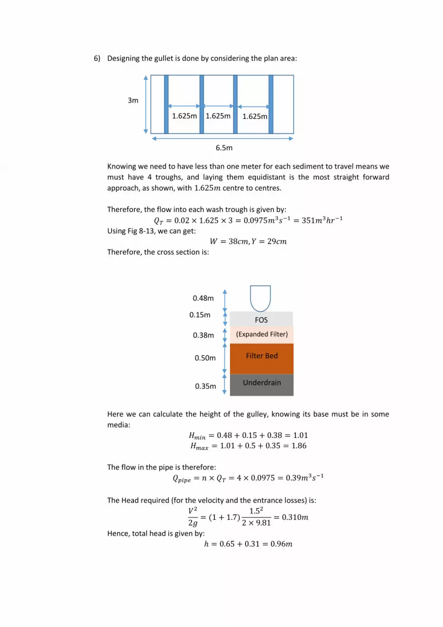
6) Designing the gullet is done by considering the plan area:
Knowing we need to have less than one meter for each sediment to travel means we
must have 4 troughs, and laying them equidistant is the most straight forward
approach, as shown, with 1.625𝑚 centre to centres.
Therefore, the flow into each wash trough is given by:
𝑄𝑇 = 0.02 × 1.625 × 3 = 0.0975𝑚3𝑠−1 = 351𝑚3ℎ𝑟−1
Using Fig 8-13, we can get:
𝑊 = 38𝑐𝑚, 𝑌 = 29𝑐𝑚
Therefore, the cross section is:
Here we can calculate the height of the gulley, knowing its base must be in some
media:
𝐻𝑚𝑖𝑛 = 0.48 + 0.15 + 0.38 = 1.01
𝐻𝑚𝑎𝑥 = 1.01 + 0.5 + 0.35 = 1.86
The flow in the pipe is therefore:
𝑄𝑝𝑖𝑝𝑒 = 𝑛 × 𝑄𝑇 = 4 × 0.0975 = 0.39𝑚3𝑠−1
The Head required (for the velocity and the entrance losses) is:
𝑉2
2𝑔= (1 + 1.7)
1.52
2 × 9.81= 0.310𝑚
Hence, total head is given by:
ℎ = 0.65 + 0.31 = 0.96𝑚
3m
6.5m
1.625m 1.625m 1.625m
Underdrain
Filter Bed
(Expanded Filter)
FOS
0.35m
0.50m
0.38m
0.15m
0.48m
𝐻 = √ℎ2 +2𝑄2
𝑔𝑏2ℎ= √0.962 +
2 × 0.392
9.81 × 𝑏2 × 0.96
This gives a number of reasonable options, e.g.:
𝑏 = 0.1, 𝐻 = 2.038
𝑏 = 0.12, 𝐻 = 1.779
𝑏 = 0.15, 𝐻 = 1.535
Given, from previous, 1.51 ≤ 𝐻 ≤ 2.36, we can suggest:
𝑏 = 0.12, 𝐻 = 1.78𝑚
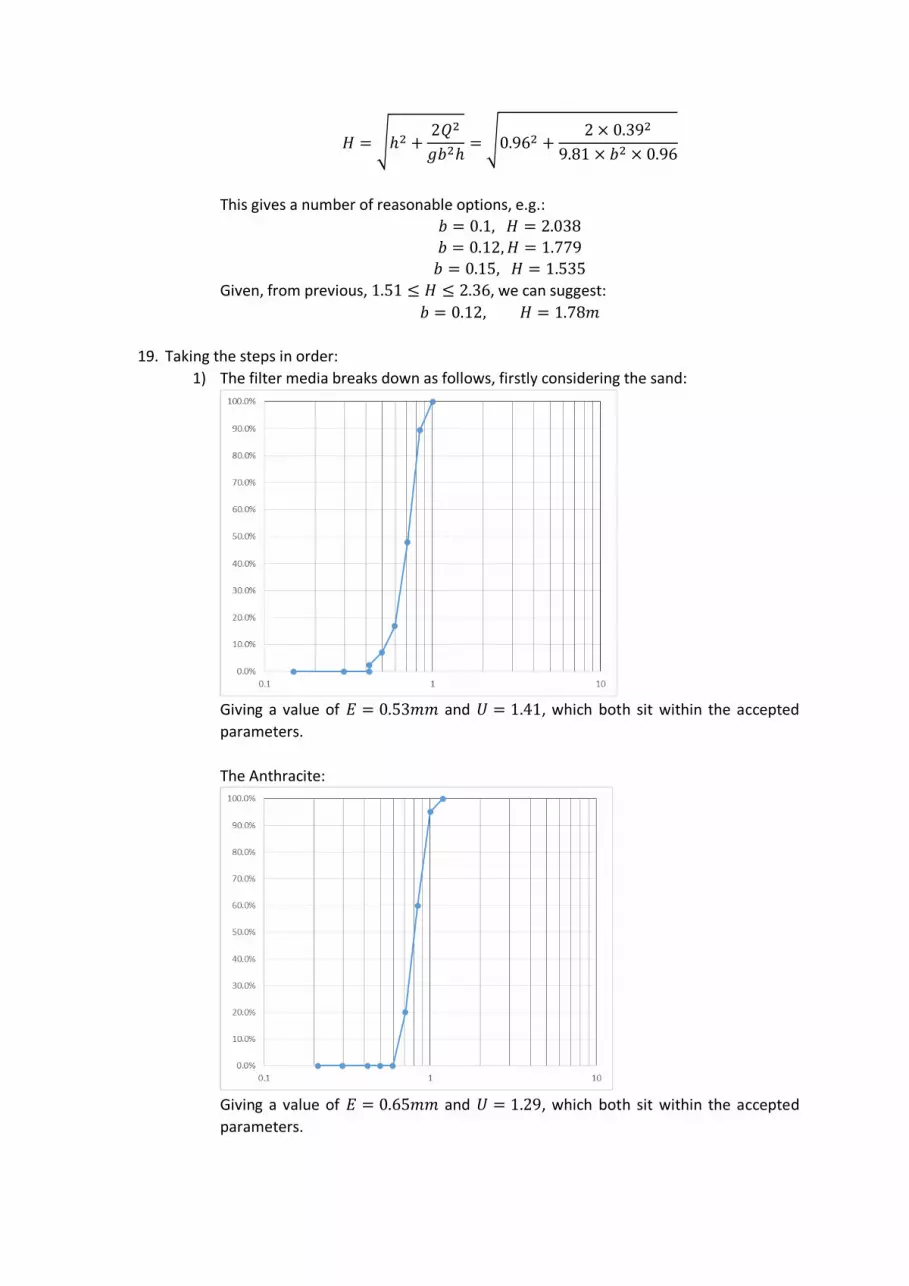
19. Taking the steps in order:
1) The filter media breaks down as follows, firstly considering the sand:
Giving a value of 𝐸 = 0.53𝑚𝑚 and 𝑈 = 1.41, which both sit within the accepted
parameters.
The Anthracite:
Giving a value of 𝐸 = 0.65𝑚𝑚 and 𝑈 = 1.29, which both sit within the accepted
parameters.

2) Knowing the flow rate and loading rate gives us:
𝑁 ≥ 0.0195√𝑄
𝑁 ≥ 0.0195 × √45000 = 4.13
As filters are constructed in pairs, we can recommend 6 filters.
𝐴 =𝑄
𝑉𝐴=
45000
15 × 24= 125
When one filter is offline, we have 5 filters operational, each requiring 25𝑚2. A
suggested plan area of 3.5𝑚 × 6.5𝑚, giving a 𝐿: 𝑊 ratio of 2.14: 1 is taken forward.
3) Considering the clean headloss – either method acceptable, but bother are shown
here for completion.
Rose:
Sand:
Size 𝒇 �̅� = √𝑑1𝑑2 𝑹𝒆 =
𝜓𝑉�̅�
𝜈
𝑪𝑫 𝑪𝑫𝒇
𝒅
18-20 0.106 0.92 2.32 12.66 1463.1 20-25 0.415 0.77 1.95 14.79 7962.5 25-30 0.311 0.65 1.64 17.31 8301.9 30-35 0.097 0.55 1.38 20.29 3608.8 35-40 0.047 0.46 1.16 23.83 2444.5 40-45 0.024 0.42 1.06 25.84 1476.9 SUM 25257.6
𝐻𝐿
𝐷=
1.067𝑉𝐹2
𝜓𝑔𝜖4∑
𝐶𝐷𝑓
𝑑
𝐻𝐿
𝐷=
1.067
0.75 × 9.81 × 0.474× (
15
602)
2
× 25257.6 = 1.303
𝐻𝐿 = 1.303 × 0.3 = 0.391𝑚
Anthracite:
Size 𝒇 �̅� = √𝑑1𝑑2 𝑹𝒆 =
𝜓𝑉�̅�
𝜈
𝑪𝑫 𝑪𝑫𝒇
𝒅
16-18 0.049 1.09 2.76 10.85 487.1 18-20 0.352 0.917 2.32 12.66 4858.5 20-25 0.410 0.771 1.95 14.79 7866.6 25-30 0.189 0.649 1.64 17.31 5045.2 SUM 18257.4
𝐻𝐿
𝐷=
1.067𝑉𝐹2
𝜓𝑔𝜖4∑
𝐶𝐷𝑓
𝑑
𝐻𝐿 = 0.355 × 0.5 = 0.178𝑚

Therefore, the total clean filter headloss is:
𝐻𝐿 = 0.391 + 0.178 = 0.569𝑚
Considering Blake-Kozeny
𝐻𝐿
𝐷=
36𝑘𝑧𝜇(1 − 𝜖)2
𝜌𝑔𝜖3𝜓2(
1
𝑛) ∑
1
𝑑2𝑉𝐹
If we split the sand into 5 parts, we get:
𝑑10 = 0.53𝑚𝑚, 𝑑30 = 0.64𝑚𝑚, 𝑑50 = 0.71𝑚𝑚, 𝑑70 = 0.78𝑚𝑚, and 𝑑90 = 0.85𝑚𝑚. We
can sum these:
∑1
𝑑2= 11.01 × 10⁶𝑚−2
Hence: 𝐻𝐿
𝐷= 1.00 ∴ 𝐻𝐿 = 1.000 × 0.3 = 0.3𝑚
Anthracite:
𝐻𝐿
𝐷=
36𝑘𝑧𝜇(1 − 𝜖)2
𝜌𝑔𝜖3𝜓2(
1
𝑛) ∑
1
𝑑2𝑉𝐹
If we split into 5 parts, we get:
𝑑10 = 0.65𝑚𝑚, 𝑑30 = 0.74𝑚𝑚, 𝑑50 = 0.81𝑚𝑚, 𝑑70 = 0.89𝑚𝑚, and 𝑑90 = 0.98𝑚𝑚. We
can sum these:
∑1
𝑑2= 7.995 × 10⁶𝑚−2
Hence: 𝐻𝐿
𝐷= 0.199 ∴ 𝐻𝐿 = 0.199 × 0.5 = 0.10𝑚
Therefore, the total clean filter headloss is:
𝐻𝐿 = 0.3 + 0.10 = 0.40𝑚
This falls within accepted parameters.
4) To find the backwash velocity, we can look at 𝑑0 of the slowest settling particles,
which will be the anthracite:
𝑑0 = 0.595𝑚𝑚
Iterating as in previous questions, we get:
𝑉𝑠 = 0.0415𝑚𝑠−1
Considering the interface:
𝑑90,𝑎 = 0.98𝑚𝑚
𝑉𝑠 = 0.076𝑚𝑠−1
𝑑10, 𝑠 = 0.53𝑚𝑚
𝑉𝑠 = 0.077𝑚𝑠−1
Hence the sand will settle faster than the anthracite, and (just) maintain stratification. Note
that there will be some blending with the finest sand grains, but this is considered acceptable

Considering the largest sand particles:
𝑑90 = 0.85𝑚𝑚
𝐺𝑎 =𝑑3𝜌𝑤𝑔(𝜌𝑠 − 𝜌𝑤)
𝜇2=
(0.85 × 10⁻³)3 × 999.5 × 9.81 × (2650 − 999.5)
(1.235 × 10⁻³)2
𝐺𝑎 = 6.52 × 10³
Hence:
𝑉𝐹 = 1.3𝑣
𝑑(√33.72 + 0.0408𝐺𝑎 − 33.7)
𝑉𝐹 = 0.0071𝑚𝑠−1
Therefore, any velocity within the bounds of 0.0071 < 𝑉𝑏 < 0.0415, provided sufficient bed
expansion occurs. Suggest 𝑉𝑏 = 0.025𝑚𝑠−1 going forward.
5) Easiest to do this in a table
Size 𝒇 �̅� = √𝑑1𝑑2 𝑹𝒆 =
𝜓𝑉𝑏�̅�
𝜈
𝑽𝒔 𝜖𝑒,𝑖 =
(𝑉𝑏
𝑉𝑠)
0.2247𝑅𝑒0.1
𝒇𝒊
1 − 𝜖𝑒,𝑖
18-20 0.106 0.92 79.12 0.142 0.602 0.266 20-25 0.415 0.77 55.81 0.119 0.638 1.147 25-30 0.311 0.65 38.85 0.099 0.679 0.968 30-35 0.097 0.55 26.62 0.080 0.723 0.350 35-40 0.047 0.46 17.90 0.064 0.773 0.207 40-45 0.024 0.42 14.59 0.057 0.799 0.120 SUM 3.06
Therefore, the expanded bed:
𝐷𝑒
𝐷= (1 − 𝜖) ∑
𝑓𝑖
1 − 𝜖𝑒, 𝑖
𝑛
𝑖=1
𝐷𝑒
𝐷= (1 − 0.47) × 3.06 = 1.62
This leads to an expanded bed of 0.487𝑚, which is comfortably within tolerance.
For the Anthracite:
Size 𝒇 �̅� = √𝑑1𝑑2 𝑹𝒆 =
𝜓𝑉𝑏�̅�
𝜈
𝑽𝒔 𝜖𝑒,𝑖 =
(𝑉𝑏
𝑉𝑠)
0.2247𝑅𝑒0.1
𝒇𝒊
1 − 𝜖𝑒,𝑖
16-18 0.049 1.09 16.56 0.086 0.693 0.159 18-20 0.352 0.92 13.92 0.071 0.737 1.336 20-25 0.410 0.77 11.71 0.058 0.785 1.909 25-30 0.189 0.65 9.85 0.047 0.839 1.174 SUM 4.578
Therefore, the expanded bed:

𝐷𝑒
𝐷= (1 − 𝜖) ∑
𝑓𝑖
1 − 𝜖𝑒, 𝑖
𝑛
𝑖=1
𝐷𝑒
𝐷= (1 − 0.6) × 4.578 = 1.83
This leads to an expanded bed of 0.92𝑚.
The total depth of expanded bed is therefore:
𝐷𝑒 = 0.92 + 0.487 = 1.407𝑚
6) Designing the gullet is done by considering the plan area:
Knowing we need to have less than one meter for each sediment to travel means we
must have 4 troughs, and laying them equidistant is the most straight forward
approach, as shown, with 1.625𝑚 centre to centres.
Therefore, the flow into each wash trough is given by:
𝑄𝑇 = 0.025 × 1.625 × 3.5 = 0.142𝑚3𝑠−1 = 512𝑚3ℎ𝑟−1
Using Fig 8-13, we can get:
𝑊 = 46𝑐𝑚, 𝑌 = 31𝑐𝑚
Therefore, the cross section is:
Here we can calculate the height of the gulley, knowing its base must be in some
media:
𝐻𝑚𝑖𝑛 = 0.54 + 0.15 + 0.61 = 1.30
𝐻𝑚𝑎𝑥 = 1.30 + 0.8 + 0.3 = 2.40
3.5m
6.5m
1.625m 1.625m 1.625m
Underdrain
Bed
(Expanded
Filter)
FOS
0.3m
0.80m
0.61m
0.15m
0.54m

The flow in the pipe is therefore:
𝑄𝑝𝑖𝑝𝑒 = 𝑛 × 𝑄𝑇 = 4 × 0.142 = 0.57𝑚3𝑠−1
The Head required (for the velocity and the entrance losses) is:
𝑉2
2𝑔= (1 + 1.7)
1.52
2 × 9.81= 0.310𝑚
Hence, total head is given by:
ℎ = 0.75 + 0.31 = 1.06𝑚
𝐻 = √ℎ2 +2𝑄2
𝑔𝑏2ℎ= √1.062 +
2 × 0.572
9.81 × 𝑏2 × 1.06
This gives a number of reasonable options, e.g.:
𝑏 = 0.15, 𝐻 = 1.98
𝑏 = 0.2, 𝐻 = 1.64
𝑏 = 0.25, 𝐻 = 1.46
Given, from previous, 1.3 ≤ 𝐻 ≤ 2.4, we can suggest:
𝑏 = 0.2, 𝐻 = 1.64𝑚
20. Taking the steps in order:
1) Selecting the material from Q12:
𝐸 = 0.42𝑚𝑚 and 𝑈 = 1.41, which both sit within the accepted parameters.
2) Knowing the flow rate and loading rate gives us:
𝑁 ≥ 0.0195√𝑄
𝑁 ≥ 0.0195 × √0.11 × 24 × 602 = 1.90
At a flow of 0.11𝑚3𝑠−1, must use 4 filters. Using a lowest filter rate is conservative
for the area required:
𝐴 =𝑄
𝑉𝐴=
0.11 × 602
5= 79.2
When one filter is offline, we require an area of 79.2𝑚2 contained within the
remaining 3 filters. Therefore:
𝐴 =79.2
3= 26.4
A suggested plan area of 3𝑚 × 9𝑚, giving a 𝐿: 𝑊 ratio of 3: 1 is taken forward.
3) Considering the clean headloss – either method acceptable, but bother are shown
here for completion.
Assuming a reasonable value of lose bed porosity of 𝜖 = 0.45, and 𝜌𝑠 = 2.65

Rose:
Size 𝒇 �̅� = √𝑑1𝑑2 𝑹𝒆 =
𝜓𝑉�̅�
𝜈
𝑪𝑫 𝑪𝑫𝒇
𝒅
16-20 0.089 1.000 1.08 25.44 2258.9 20-30 0.315 0.707 0.76 35.19 15654.2 30-40 0.510 0.500 0.54 48.87 49876.3 40-50 0.086 0.353 0.38 68.11 16642.3 SUM 84431.7
𝐻𝐿
𝐷=
1.067𝑉𝐹2
𝜓𝑔𝜖4∑
𝐶𝐷𝑓
𝑑
𝐻𝐿
𝐷= 0.527
𝐻𝐿 = 0.527 × 0.8 = 0.422𝑚
Considering Blake-Kozeny
𝐻𝐿
𝐷=
36𝑘𝑧𝜇(1 − 𝜖)2
𝜌𝑔𝜖3𝜓2(
1
𝑛) ∑
1
𝑑2𝑉𝐹
If we split the sand into 5 parts, we get:
𝑑10 = 0.42𝑚𝑚, 𝑑30 = 0.49𝑚𝑚, 𝑑50 = 0.56𝑚𝑚, 𝑑70 = 0.68𝑚𝑚, and 𝑑90 = 0.83𝑚𝑚. We
can sum these:
∑1
𝑑2= 16.453 × 10⁶𝑚−2
Hence: 𝐻𝐿
𝐷= 0.437 ∴ 𝐻𝐿 = 0.437 × 0.8 = 0.350𝑚
This falls within accepted parameters.
4) To find the backwash velocity, we look at 𝑑0 (as Q12)
𝑑0 = 0.297𝑚𝑚
𝑉𝑠 = 0.0366𝑚𝑠−1
Considering the larger particles:
𝑑90 = 0.83𝑚𝑚
𝐺𝑎 =𝑑3𝜌𝑤𝑔(𝜌𝑠 − 𝜌𝑤)
𝜇2=
(0.83 × 10⁻³)3 × 998.599 × 9.81 × (2650 − 998.599)
(1.053 × 10⁻³)2
𝐺𝑎 = 8342
Hence:
𝑉𝐹 = 1.3𝑣
𝑑(√33.72 + 0.0408𝐺𝑎 − 33.7)
𝑉𝐹 = 1.31.054 × 10−6
0.83 × 10⁻³(√33.72 + 0.0408 × 8342.4 − 33.7)
𝑉𝐹 = 0.0078𝑚𝑠−1
Therefore, any velocity within the bounds of 0.0078 < 𝑉𝑏 < 0.037, provided sufficient bed
expansion occurs. Suggest 𝑉𝑏 = 0.018𝑚𝑠−1 going forward.

5) Easiest to do this in a table
Size 𝒇 �̅� = √𝑑1𝑑2 𝑹𝒆 =
𝜓𝑉𝑠�̅�
𝜈
𝑽𝒔 𝜖𝑒,𝑖 =
(𝑉𝑏
𝑉𝑠)
0.2247𝑅𝑒0.1
𝒇𝒊
1 − 𝜖𝑒,𝑖
16-20 0.089 1.000 14.02 0.165 0.523 0.186 20-30 0.315 0.707 9.92 0.119 0.586 0.761 30-40 0.510 0.500 7.01 0.081 0.663 1.511 40-50 0.086 0.353 4.95 0.052 0.756 0.353 SUM 2.811
Therefore, the expanded bed:
𝐷𝑒
𝐷= (1 − 𝜖) ∑
𝑓𝑖
1 − 𝜖𝑒, 𝑖
𝑛
𝑖=1
𝐷𝑒
𝐷= (1 − 0.45) × 2.811 = 1.55
This leads to an expanded bed of 1.24𝑚, which is comfortably within tolerance.
6) Designing the gullet is done by considering the plan area:
Knowing we need to have less than one meter for each sediment to travel means we
must have 5 troughs, and laying them equidistant is the most straight forward
approach, as shown, with 1.8𝑚 centre to centres.
Therefore, the flow into each wash trough is given by:
𝑄𝑇 = 0.018 × 1.8 × 3 = 0.0972𝑚3𝑠−1 = 350𝑚3ℎ𝑟−1
Using Fig 8-13, we can get:
𝑊 = 38𝑐𝑚, 𝑌 = 29𝑐𝑚
Therefore, the cross section is:
3m
9m
1.8m 1.8m 1.8m
Underdrain
Bed
(Expanded
Filter)
FOS
0.20m
0.80m
0.44m
0.15m
0.48m
1.8m

Here we can calculate the height of the gulley, knowing its base must be in some
media:
𝐻𝑚𝑖𝑛 = 0.48 + 0.15 + 0.44 = 1.07
𝐻𝑚𝑎𝑥 = 1.07 + 0.8 + 0.2 = 2.07
The flow in the pipe is therefore:
𝑄𝑝𝑖𝑝𝑒 = 𝑛 × 𝑄𝑇 = 5 × 0.0975 = 0.49𝑚3𝑠−1
The diameter of the pipe can be approximated:
𝑑 = (𝑄
𝑉×
4
𝜋)
0.5
= (0.49
1×
4
𝜋)
0.5
= 0.79
If we conservatively assume a 1𝑚 diameter pipe:
The Head required (for the velocity and the entrance losses) is:
𝑉2
2𝑔= (1 + 1.7)
12
2 × 9.81= 0.14𝑚
Hence, total head is given by:
ℎ = 1 + 0.14 = 1.14𝑚
𝐻 = √ℎ2 +2𝑄2
𝑔𝑏2ℎ= √1.142 +
2 × 0.492
9.81 × 𝑏2 × 1.14
This gives a number of reasonable options, e.g.:
𝑏 = 0.15, 𝐻 = 1.79
𝑏 = 0.2, 𝐻 = 1.540
𝑏 = 0.25, 𝐻 = 1.409
Given, from previous, 1.07 ≤ 𝐻 ≤ 2.07, we can suggest any of these, so picking a
reasonable value:
𝑏 = 0.2, 𝐻 = 1.54𝑚