A Steady state management of multi species fisheries: the case of malaysiaNik Hashim Nik Mustapha

Department of EconomicsFaculty of Management and EconomicsUMT, Kuala Terengganu.

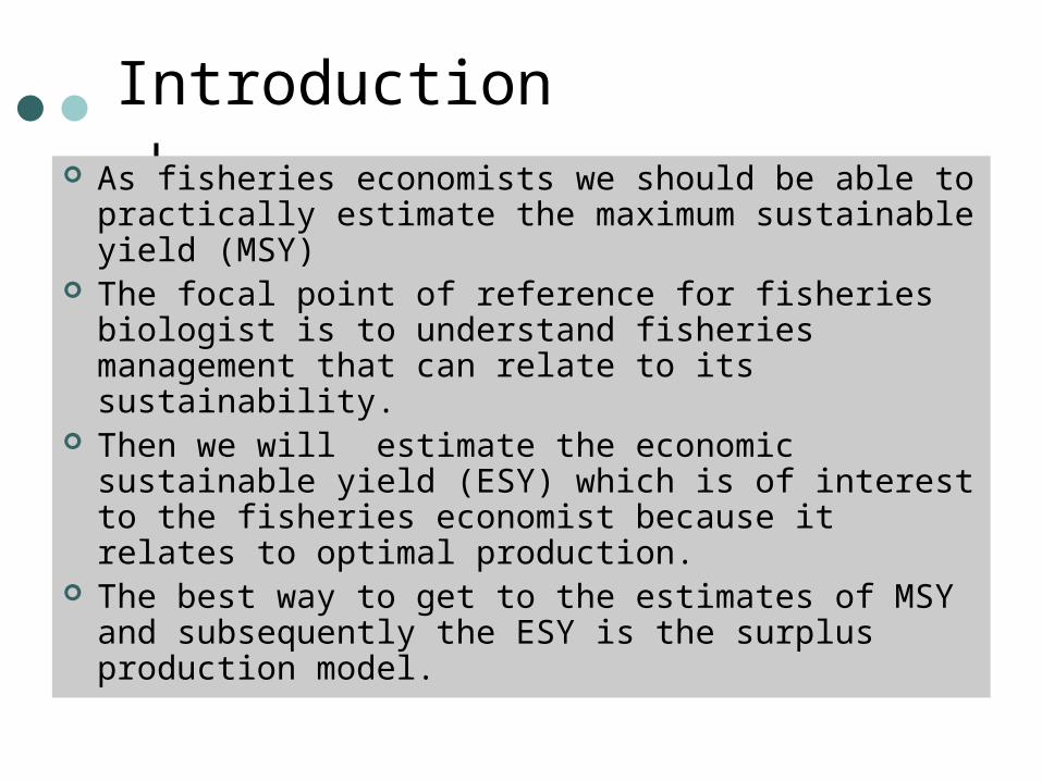
Introduction As fisheries economists we should be able to practically estimate the maximum sustainable yield (MSY)

The focal point of reference for fisheries biologist is to understand fisheries management that can relate to its sustainability.

Then we will estimate the economic sustainable yield (ESY) which is of interest to the fisheries economist because it relates to optimal production.

The best way to get to the estimates of MSY and subsequently the ESY is the surplus production model.

Fisheries Production Models

This fisheries model is known under many names: production model, stock production model, surplus yield model, bionomic model and biomass dynamic model (Jennings et al. 2001 p.128).

You can develop the surplus production modal or the Schaefer’s production model mathematically (refer Nik Hashim N M and Nik Fuad N M K 2006).

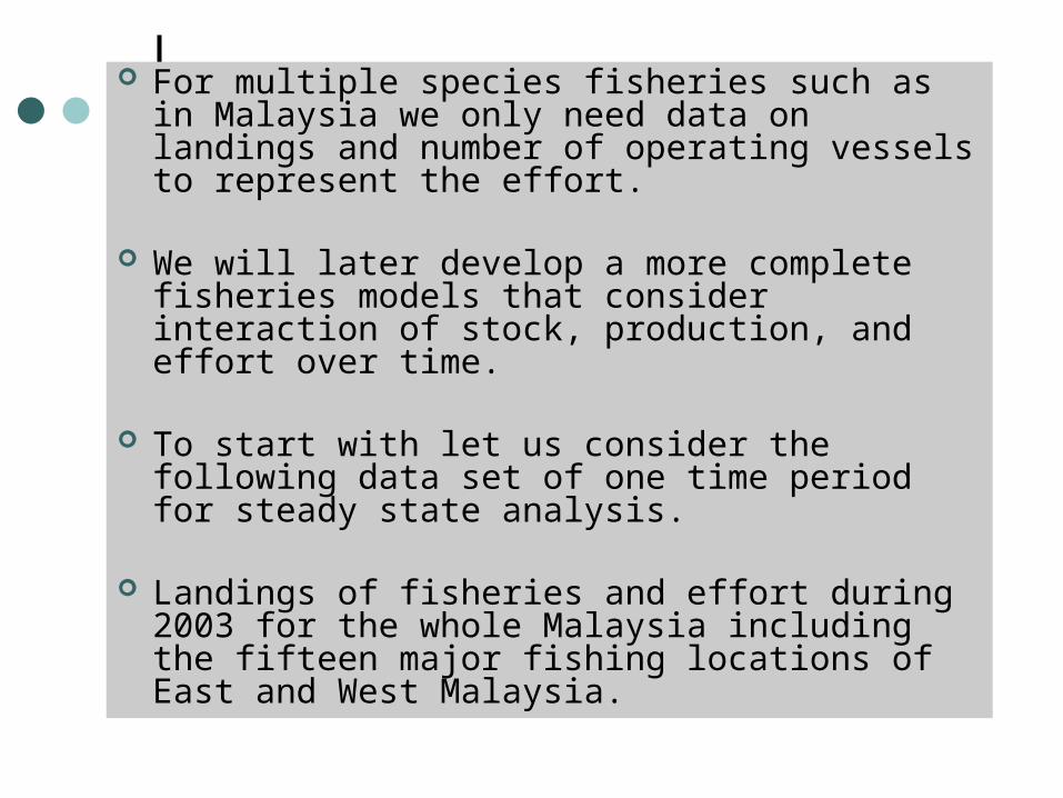
For multiple species fisheries such as in Malaysia we only need data on landings and number of operating vessels to represent the effort.

We will later develop a more complete fisheries models that consider interaction of stock, production, and effort over time.

To start with let us consider the following data set of one time period for steady state analysis.

Landings of fisheries and effort during 2003 for the whole Malaysia including the fifteen major fishing locations of East and West Malaysia.

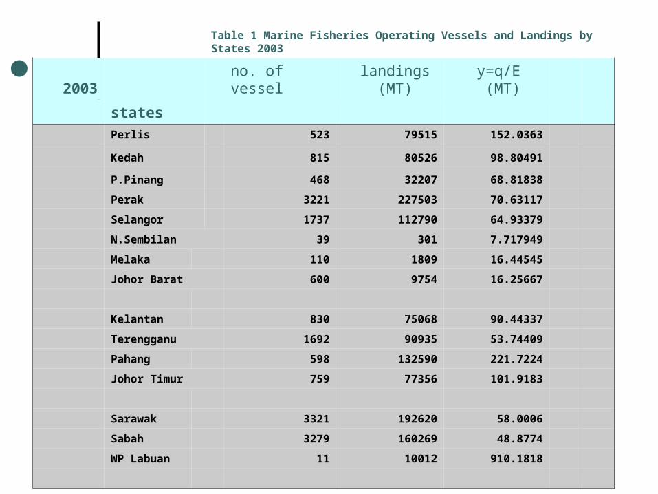
Table 1 Marine Fisheries Operating Vessels and Landings by States 2003

2003    no. of vessel

landings (MT)

y=q/E (MT)    

  states            

  Perlis   523 79515 152.0363    

  Kedah   815 80526 98.80491    

  P.Pinang   468 32207 68.81838    

  Perak   3221 227503 70.63117    

  Selangor   1737 112790 64.93379    

  N.Sembilan 39 301 7.717949    

  Melaka   110 1809 16.44545    

  Johor Barat 600 9754 16.25667    

               

  Kelantan   830 75068 90.44337    

  Terengganu 1692 90935 53.74409    

  Pahang   598 132590 221.7224    

  Johor Timur 759 77356 101.9183    

               

  Sarawak   3321 192620 58.0006    

  Sabah   3279 160269 48.8774    

  WP Labuan   11 10012 910.1818    

               

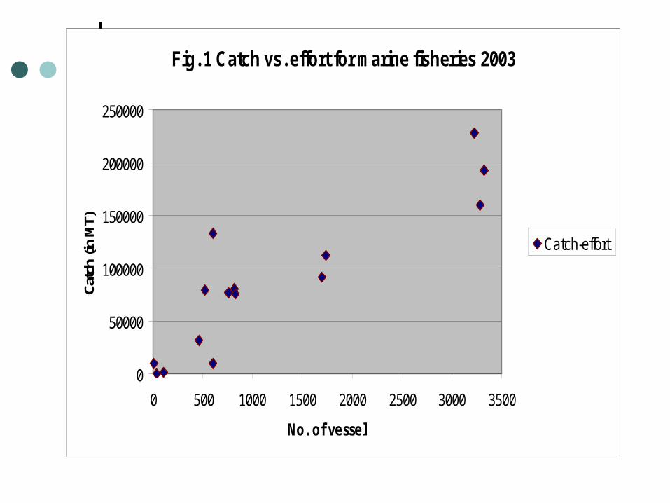
Fig. 1 Catch vs. effort for m arine fisheries 2003

0

50000

100000

150000

200000

250000

0 500 1000 1500 2000 2500 3000 3500No. of vessel

Catch (in MT)

Catch-effort

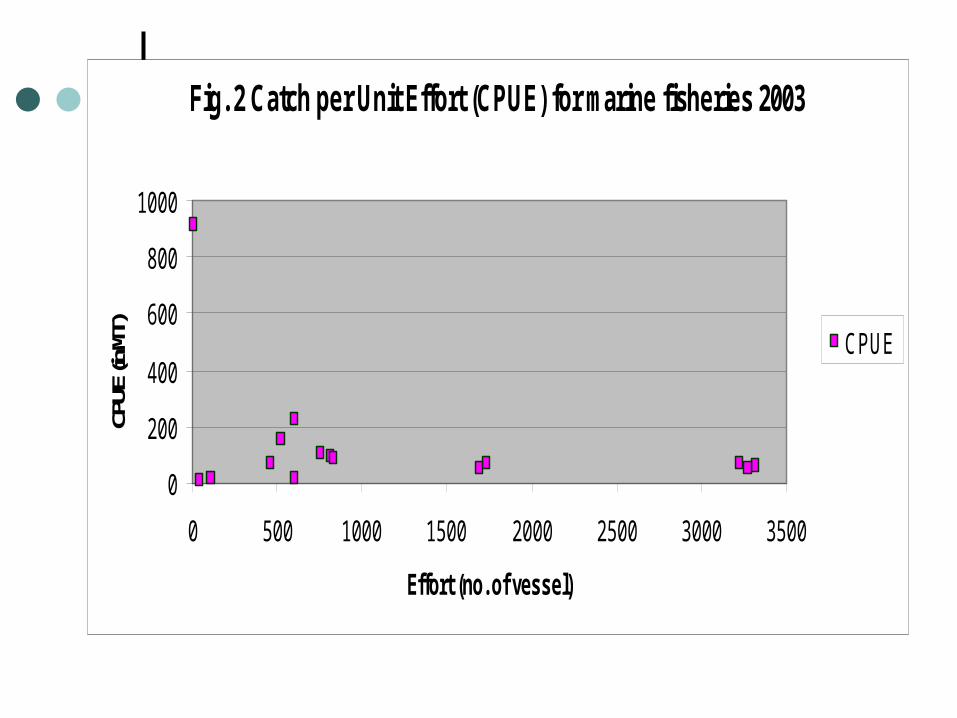
Fig. 2 Catch per Unit Effort (CPUE) for m arine fisheries 2003

02004006008001000

0 500 1000 1500 2000 2500 3000 3500Effort (no. of vessel)

CPUE (in MT) CPUE

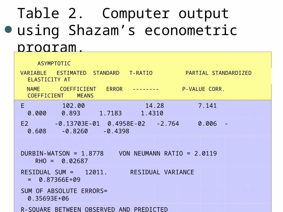
Table 2. Computer output using Shazam’s econometric program.

ASYMPTOTIC          

VARIABLE ESTIMATED STANDARD T-RATIO PARTIAL STANDARDIZED ELASTICITY AT

NAME COEFFICIENT ERROR -------- P-VALUE CORR. COEFFICIENT MEANS  

E 102.00 14.28 7.141 0.000 0.893 1.7183 1.4310  

E2 -0.13703E-01 0.4958E-02 -2.764 0.006 -0.608 -0.8260 -0.4398  

                     

DURBIN-WATSON = 1.8778 VON NEUMANN RATIO = 2.0119 RHO = 0.02687    

RESIDUAL SUM = 12011. RESIDUAL VARIANCE = 0.87366E+09      

SUM OF ABSOLUTE ERRORS= 0.35693E+06            

R-SQUARE BETWEEN OBSERVED AND PREDICTED = 0.8104        

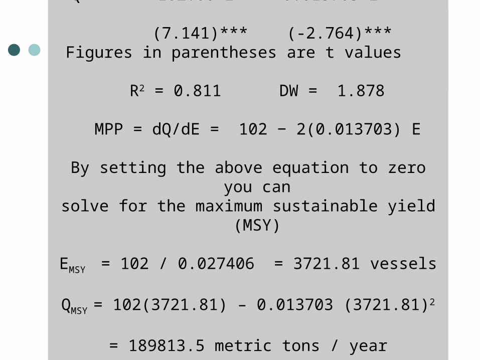
Derivation of MSY and ESY

Q = 102.00 E − 0.013703 E2

(7.141)*** (-2.764)*** Figures in parentheses are t values

R2 = 0.811 DW = 1.878

MPP = dQ/dE = 102 − 2(0.013703) E

By setting the above equation to zero you can

solve for the maximum sustainable yield (MSY)

EMSY = 102 / 0.027406 = 3721.81 vessels

QMSY = 102(3721.81) – 0.013703 (3721.81)2

= 189813.5 metric tons / year

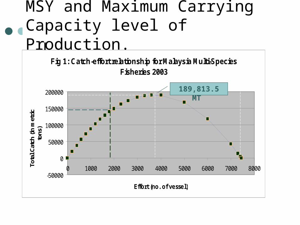
MSY and Maximum Carrying Capacity level of Production.

Fig 1: Catch-effort relationship for M alaysia M ulti-Species Fisheries 2003

-50000

0

50000

100000

150000

200000

0 1000 2000 3000 4000 5000 6000 7000 8000

Effort (no. of vessel)

Total Catch (in metric

tons)

189,813.5 MT

-150

-100

-50

0

50

100

150

0 2000 4000 6000 8000

Effort (no. of vessel)

MPP

&AP

P

MPPAPP

3,721.8

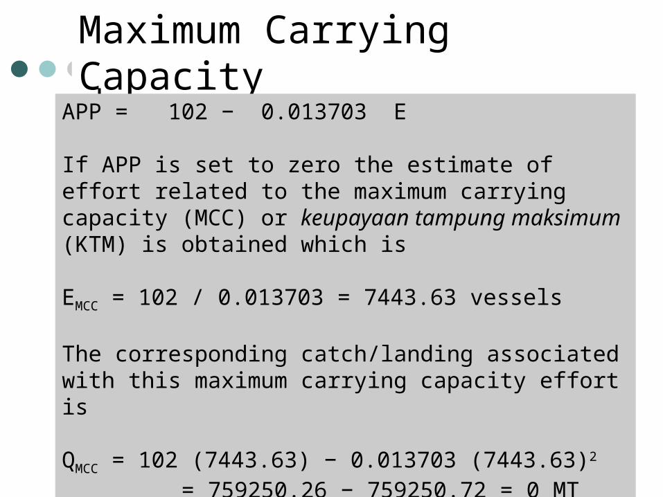
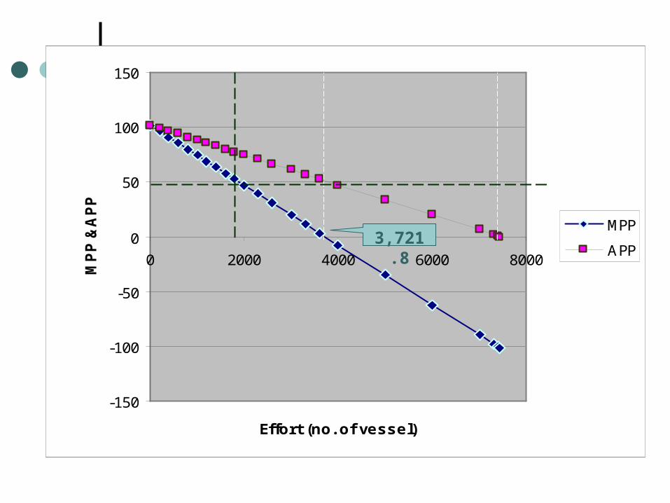
Maximum Carrying Capacity

APP = 102 − 0.013703 E

If APP is set to zero the estimate of effort related to the maximum carrying capacity (MCC) or keupayaan tampung maksimum (KTM) is obtained which is

EMCC = 102 / 0.013703 = 7443.63 vessels

The corresponding catch/landing associated with this maximum carrying capacity effort is

QMCC = 102 (7443.63) − 0.013703 (7443.63)2 = 759250.26 − 759250.72 = 0 MT per annum.

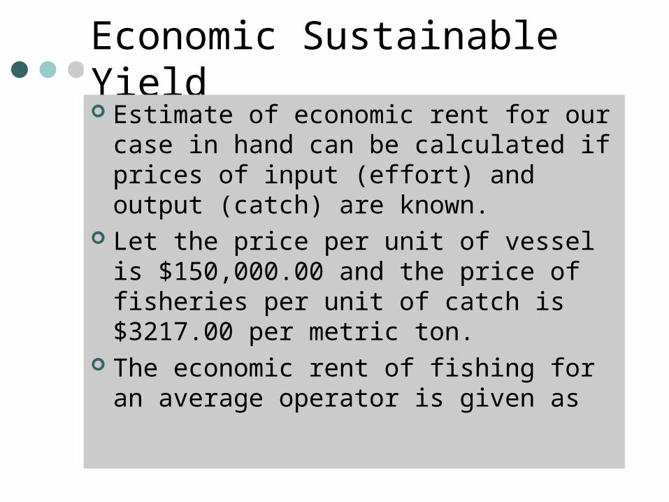
Economic Sustainable Yield Estimate of economic rent for our case in hand can be calculated if prices of input (effort) and output (catch) are known.

Let the price per unit of vessel is $150,000.00 and the price of fisheries per unit of catch is $3217.00 per metric ton.

The economic rent of fishing for an average operator is given as

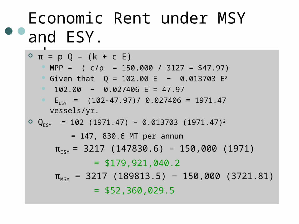
Economic Rent under MSY and ESY. π = p Q – (k + c E)

MPP = ( c/p = 150,000 / 3127 = $47.97) Given that Q = 102.00 E − 0.013703 E2

102.00 − 0.027406 E = 47.97 EESY = (102-47.97)/ 0.027406 = 1971.47 vessels/yr.

QESY = 102 (1971.47) − 0.013703 (1971.47)2 = 147, 830.6 MT per annumπESY = 3217 (147830.6) − 150,000 (1971) = $179,921,040.2

πMSY = 3217 (189813.5) − 150,000 (3721.81) = $52,360,029.5

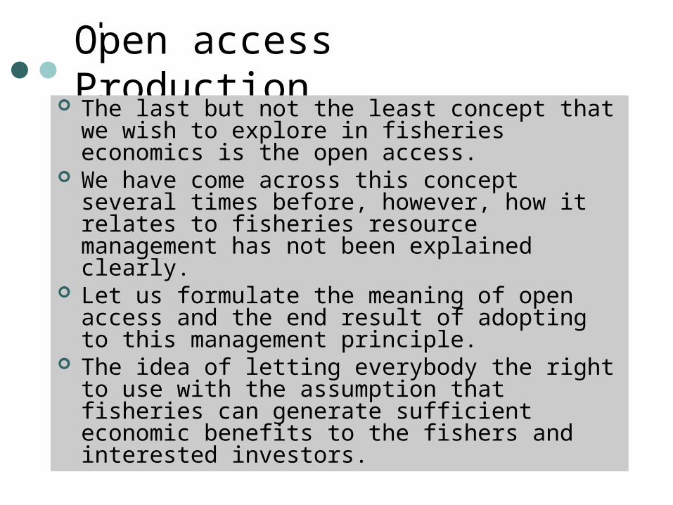
Open access Production The last but not the least concept that we wish to explore in fisheries economics is the open access.

We have come across this concept several times before, however, how it relates to fisheries resource management has not been explained clearly.

Let us formulate the meaning of open access and the end result of adopting to this management principle.

The idea of letting everybody the right to use with the assumption that fisheries can generate sufficient economic benefits to the fishers and interested investors.

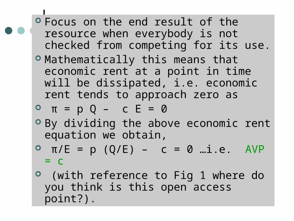
Focus on the end result of the resource when everybody is not checked from competing for its use.

Mathematically this means that economic rent at a point in time will be dissipated, i.e. economic rent tends to approach zero as

π = p Q – c E = 0 By dividing the above economic rent equation we obtain,

π/E = p (Q/E) – c = 0 …i.e. AVP = c

(with reference to Fig 1 where do you think is this open access point?).

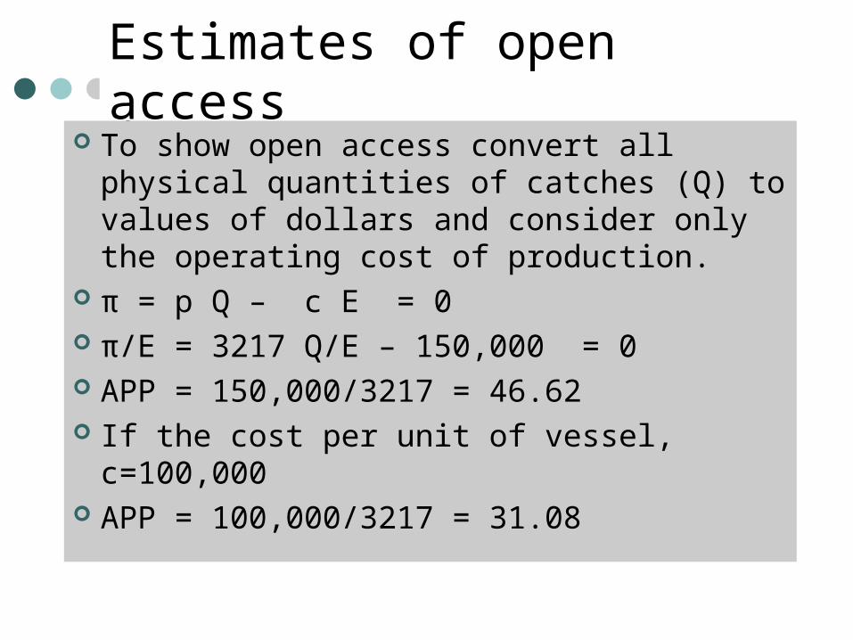
Estimates of open access

To show open access convert all physical quantities of catches (Q) to values of dollars and consider only the operating cost of production.

π = p Q – c E = 0 π/E = 3217 Q/E – 150,000 = 0 APP = 150,000/3217 = 46.62 If the cost per unit of vessel, c=100,000

APP = 100,000/3217 = 31.08

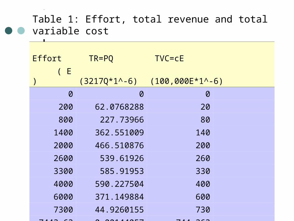
Table 1: Effort, total revenue and total variable cost Effort TR=PQ TVC=cE  

( E ) (3217Q*1^-6) (100,000E*1^-6)

0 0 0  

200 62.0768288 20  

800 227.73966 80  

1400 362.551009 140  

2000 466.510876 200  

2600 539.61926 260  

3300 585.91953 330  

4000 590.227504 400  

6000 371.149884 600  

7300 44.9260155 730  

7443.63 -0.00144057 744.363  

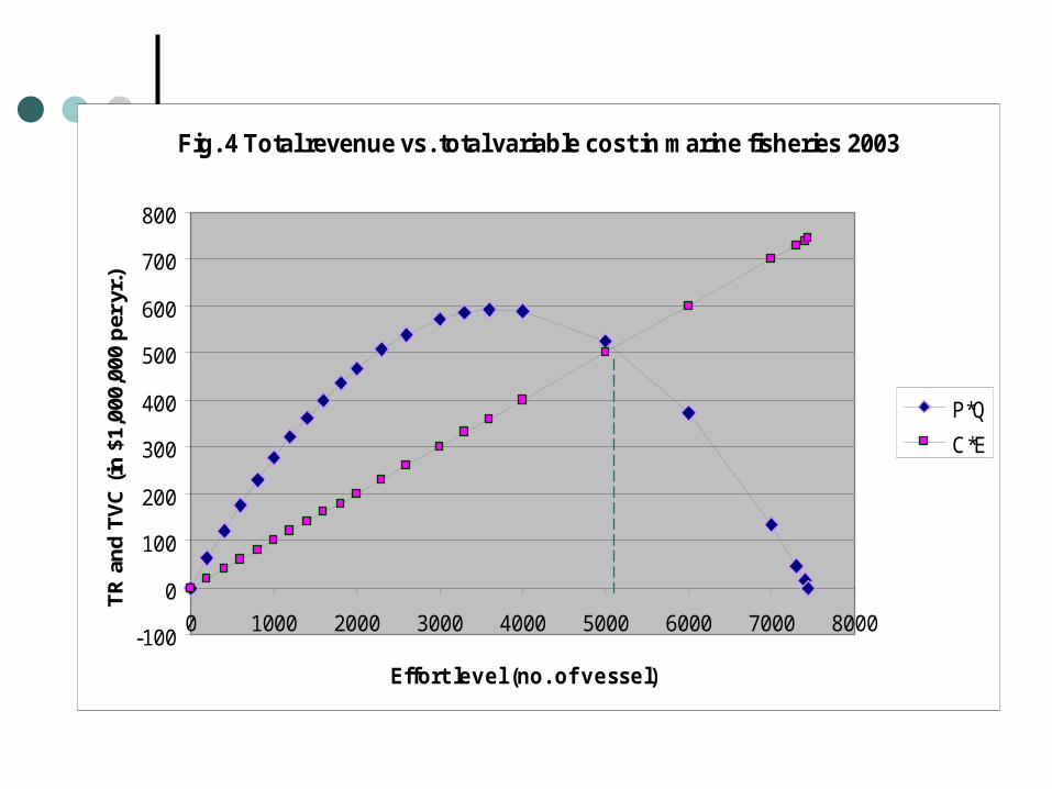
Fig. 4 Total revenue vs. total variable cost in m arine fisheries 2003

-100

0

100

200

300

400

500

600

700

800

0 1000 2000 3000 4000 5000 6000 7000 8000

Effort level (no. of vessel)

TR and TVC

(in $1,000,000 per yr.)

P*QC*E

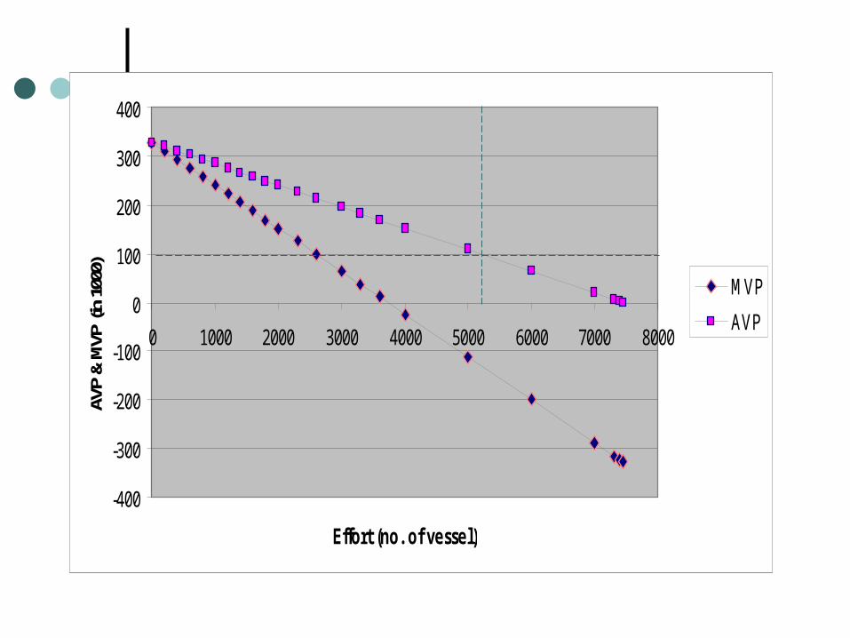
-400

-300

-200

-100

0

100

200

300

400

0 1000 2000 3000 4000 5000 6000 7000 8000

Effort (no. of vessel)

AVP & MVP (in 1000)

M VPAVP

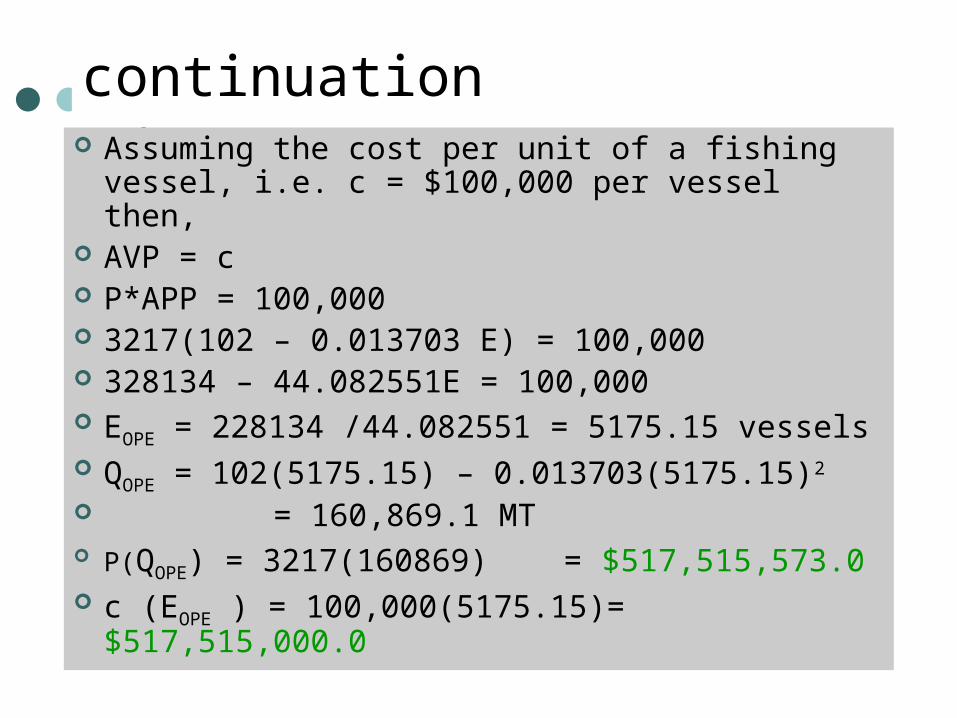
continuation Assuming the cost per unit of a fishing vessel, i.e. c = $100,000 per vessel then,

AVP = c P*APP = 100,000 3217(102 – 0.013703 E) = 100,000 328134 – 44.082551E = 100,000 EOPE = 228134 /44.082551 = 5175.15 vessels QOPE = 102(5175.15) – 0.013703(5175.15)2

= 160,869.1 MT P(QOPE) = 3217(160869) = $517,515,573.0 c (EOPE ) = 100,000(5175.15)= $517,515,000.0

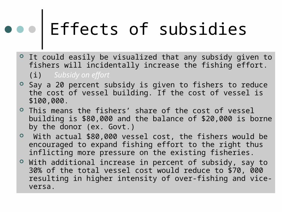
Effects of subsidies It could easily be visualized that any subsidy given to

fishers will incidentally increase the fishing effort.(i) Subsidy on effort

Say a 20 percent subsidy is given to fishers to reduce the cost of vessel building. If the cost of vessel is $100,000.

This means the fishers’ share of the cost of vessel building is $80,000 and the balance of $20,000 is borne by the donor (ex. Govt.)

With actual $80,000 vessel cost, the fishers would be encouraged to expand fishing effort to the right thus inflicting more pressure on the existing fisheries.

With additional increase in percent of subsidy, say to 30% of the total vessel cost would reduce to $70, 000 resulting in higher intensity of over-fishing and vice-versa.

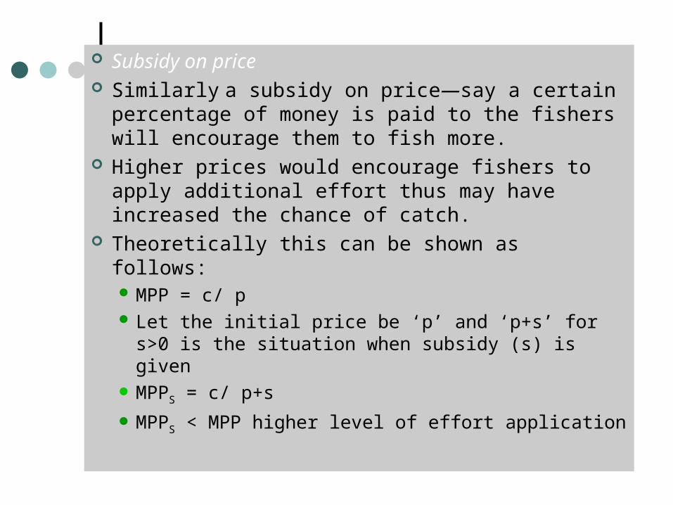
Subsidy on price Similarly a subsidy on price—say a certain percentage of money is paid to the fishers will encourage them to fish more.

Higher prices would encourage fishers to apply additional effort thus may have increased the chance of catch.

Theoretically this can be shown as follows: MPP = c/ p Let the initial price be ‘p’ and ‘p+s’ for s>0 is the situation when subsidy (s) is given

MPPS = c/ p+s MPPS < MPP higher level of effort application

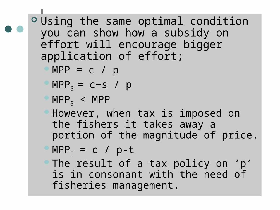
Using the same optimal condition you can show how a subsidy on effort will encourage bigger application of effort;MPP = c / pMPPS = c−s / pMPPS < MPPHowever, when tax is imposed on the fishers it takes away a portion of the magnitude of price.

MPPT = c / p-tThe result of a tax policy on ‘p’ is in consonant with the need of fisheries management.

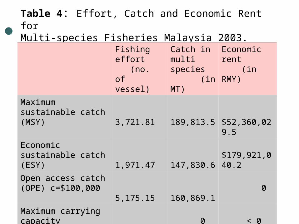
Table 4: Effort, Catch and Economic Rent forMulti-species Fisheries Malaysia 2003.

Fishing effort (no. of vessel)

Catch in multi species (in MT)

Economic rent (in RMY)

Maximum sustainable catch(MSY)

3,721.81

189,813.5

$52,360,029.5

Economic sustainable catch(ESY)

1,971.47

147,830.6

$179,921,040.2

Open access catch(OPE) c=$100,000

5,175.15

160,869.1

0

Maximum carrying capacity(MCC)

7,443.63

0

< 0

Conclusion Before we end this topic on the steady-state fisheries management you should be able to understand some of the basic concepts in fisheries economics.

By now you should be able to analyze and interpret the general form of the fisheries catch-effort function.

To test your generic skill associated with the analytical competence/ability we suggest that you try to derive all the concepts discussed this section.