determining countries’ tax effort
TRANSCRIPT
Hacienda Puacuteblica Espantildeola Revista de Economiacutea Puacuteblica 195shy(42010) 65shy87 copy 2010 Instituto de Estudios Fiscales
Determining countriesrsquo tax effort
CAROLA PESSINO Universidad Torcuato Di Tella
RICARDO FENOCHIETTO Fiscal Affairs Department International Monetary Fund (IMF)
Recibido Mayo 2010 Aceptado Noviembre 2010
Abstract
This paper presents a model to determine the tax effort and tax capacity of 96 countries and the main varishyables from which they depend The results and the model allow us to clearly determine which countries are near their tax capacity and which are some way from it and therefore could increase their tax revenue Our study corroborates previous analysis inasmuch as the positive and significant relationship between tax revenue as percent of GDP and the level of development (per capita GDP) trade (imports and exports as percent of GDP) and education (public expenditure on education as percent of GDP) The study also demonstrates the negative relationship between tax revenue and inflation (CPI) income distribution (GINI coefficient) the ease of tax collection (agricultural sector value added as GDP percent) and corruption
Keywords tax effort tax frontier tax capacity tax revenue stochastic tax frontier inefficiency
JEL classification C23 C51 H2 H21
1 Introduccioacuten
While tax capacity represents the maximum tax revenue that a country can collect given its economic social institutional and demographic characteristics tax effort is the relation between the actual revenue and this tax capacity This paper presents a model to build a lsquostochastic tax frontierrsquo to determine the tax effort of 96 countries from which data were available This model is also useful to measure the main variables from which tax capacity and tax effort depend on
The authors benefited from the comments and support provided by John Norregaard Helpful comments and guidance were also provided by anonymous referees Universidad Torcuato Di Tella Buenos aires Argentina eshymail epessinoutdtedu Fiscal Affaairs Department International Monetary Fund (IMF) Washington eshymail rfenochiettoimforg The views expressed herein are those of the authors and should not be attributed to the IMF its Executive Board or its management
66 CAROLA PESSINO AND RICARDO FENOCHIETTO
The results and the model allow us to clearly determine which countries are near their tax capacity and which are some way from it and therefore could increase their tax revenue
To know countriesrsquo tax effort is crucial in tax policy because this allows knowing what countries can increase their tax revenue and what countries cannot The initial step that countries should follow before implementing new taxes or increasing the rate of the existing ones is to analyze how far their actual revenue is from their tax capacity If a country needs resources to increase its public expenditure and it is very near its tax capacity it will not be able increase taxes and therefore it will have to look for another source of financing or renounce to such increase of expenditure
There are only few papers that study tax effort and tax capacity and most of them only cover a limited group of countries usually ones that belong to a specific region One of the main advantages of our study is that includes most countries around the world This is particularly important because to predict tax effort we use a relative method using the comparative analysis of data on these countries
This paper is organized as follows Section 2 defines what tax effort is and particularly compares it with other common measures such as potential tax revenue and actual tax revenue Section 3 presents a brief review of related literature Section 4 develops the idea of stochastic frontier production the model utilized in our research Section 5 explains the estimation strategy Section 6 the variables chosen (as dependent and independent) and describes the available data for this study Section 7 compares and analyses the most significant results Finally section 8 includes the main conclusions
2 Tax effort and other definitions
The following are some definitions that are useful to understand our study While tax capacity represents the maximum tax revenue that could be collected in a country given its economic social institutional and demographic characteristics potential tax collection represents the maximum revenue that could be obtained through the law tax system Tax gap is the difference between this potential tax collection and the actual revenue which is a function of tax capacity and the extent to which by tax laws and administration a society wishes to mobilize resources for public use
Tax effort is the ratio between actual revenue and tax capacity It is better to call this ratio tax effort rather than tax efficiency Some countries can be efficient and have a lower level of collection and be far from their tax capacity because they simply choose to levy lower taxes and to provide a low level of public goods and services that is to have a small government
In our model having a low tax effort only means that this tax effort is relatively low compared to that of other countries It does not necessarily mean that this country is inefficient in collecting taxes or that it has to increase its revenue
67 Determining countriesrsquo tax effort
3 Brief review of related literature
Only a few papers study tax effort and most of them employ cross section empirical methods and hence ignore the variation over time Some of these papers have aimed at identifying the determinants of the level of taxation Lotz and Mors (1967) published one of the first articles to study the international tax ratio As explanatory variables they used the level of development represented by per capita Gross National Product (GNP) and trade represented by exports plus imports to total GNP
Varsano et al (1998) using a regression model concluded that the tax effort developed by Brazilian society was relatively high well above the average for a sample of countries considered Furthermore as there was a large unmet demand for government services and investment it was expected that even counting on the success of efforts to restrict public expenditure the tax burden in this country still remained high for a long period
Afirman (2003) carried out a different study that included only one country (Indonesia) to conclude that all local governments could maximize their tax revenue According to this study property tax collection could increase by 020 percent of Gross Domestic Product (GDP) and other local taxes by 010 percent while current total local tax revenue was 036 percent of GDP
Gupta (2007) used regression analysis in a dynamic panel data model and he found that some structural factors such as per capita GDP agriculturersquos share in GDP trade openness and foreign aid significantly affect revenue and while several Sub Saharan African countries are performing well above their potential some Latin American economies fall short of their revenue potential
Davoodi and Grigorian (2007) who also used a regression framework extend the conventional determinants of tax potential to include measures of institutional quality and shadow economy in a panel data framework The empirical analysis of this paper shows that in Armenia improvement in institutions as well as policy measures designed to reduce the size of the shadow economy are important factors in boosting tax performance
While most studies cover only a limited group of countries usually belonging to a specific region our study includes most countries around the world The scope of our study is particularly important because we use a relative method to predict tax efficiency That is to say taking into account several characteristics the method determines if a countryrsquos tax capacity is high or low in comparison with the tax capacity of the other countries
Other innovation of our study with regard to the previous papers consists in the use of a tax stochastic frontier model influencing timeshyvarying inefficiency with two disturbances terms one that allows distinguishing the existences of technical inefficiencies and the other the usual mean zero statistical error term
68 CAROLA PESSINO AND RICARDO FENOCHIETTO
4 Stochastic tax frontier
Tax frontier development is similar to production frontier development but with two main differences First in frontier production the output is produced by specific inputs labor capital and land As Afirman (2003) expresses in this case the determinants of output are very clear they are all inputs used in production However the situation may be less clear for tax frontier estimation It is clear that per capita GDP or some related economic indicators such as level of education are inputs of revenue collection It is not so clear that inflation and GINI coefficient are inputs an issue that we will consider later
Second main difference is the interpretation of the results In production frontier the difference between current production and frontier represents the level of inefficiency something that firms do not accomplish In tax frontier the difference between actual revenue and tax capacity includes the existence of technical inefficiencies as well as policy issues (differences in tax legislation for instance in the level of tax rates)
The stochastic frontier tax function is an extension of the familiar regression model based on the theoretical premise that a production function represents the maximum output (level of tax revenue) that a country can achieve considering a set of inputs (GDP per capita inflation level of education and so on)
The stochastic frontier model of Aigner Lovell and Schmidt (1977) is the standard econometric platform for this analysis A panel version of this model can be written as
ln τ it =α+βT xit + vit minus uit [1]
where
uit = represents the inefficiency the ldquofailurerdquo to produce the relative maximum level of tax collection or production It is a nonshynegative random variable associated with countryshyspecific factors which contribute to country i not attaining its tax capacity at time t
uit gt 0 = but vit may take any value τ = it represents the tax capacity to GDP ratio for country i at time t xit = represents variables affecting tax revenue for country i at time t β = is avector of unknown parameters vit = is the statistical noise known as the disturbance or error term It is a random
(stochastic) variable which represents all those independent variables that affect the dependent one but are not explicitly taken into account as well as measurement errors and incorrect functional form vit can be positive or negative and so the stochastic frontier outputs vary on the deterministic part of the model
It is usually assumed that
69 Determining countriesrsquo tax effort
a) vit has a symmetric distribution such as the normal distribution and b) vi and ui are statistically independent of each other
Figure 1 illustrates the main characteristics of the frontier model considering only one independent variable from which tax capacity depends on If this is the case the model takes the following form
ln τ =β +β x v u [2] + minusi 0 1 i i i
where β0 + β1 xi is the deterministic component vi is the noise and ui is the inefficiency
The horizontal axis of figure 1 represents the values of inputs (log of GDP and so on) and the vertical axis the values of the output (log of tax effort) Points A and B shows the actual tax revenue of two countries (A and B) Without inefficiencies country A would collect C and country B would collect D For country A the noise effect is positive and then its frontier revenue is above the deterministic frontier revenue function On the other hand for Country B the noise effect is negative and then its revenue frontier is under the deterministic frontier revenue function 1
While frontier revenues are distributed above and below the deterministic frontier revenue function actual tax revenues are always below this function because the noise effect is positive and larger than the inefficiency effect
Figure 1 The Stochastic Production Frontier
The analysis aims to predict and measure inefficiency effects To do so we use the tax effort defined as the ratio between actual tax revenue and the corresponding stochastic frontier tax revenue (tax capacity) This measure of tax effort has a value between zero and one
70 CAROLA PESSINO AND RICARDO FENOCHIETTO
Tτ it exp (( + xit vit itα β + minusu )TE = = = exp minusu [3]( )it itT Texp α β x + v ) exp α β x + v )( + it it ( + it it
The difference between current tax revenue and tax frontier can be interpreted only as the level of unused tax but not strictly as a measure of inefficiency The presence of unused tax may be caused by two factors peoplersquos preferences of low provision of public goods and services so the low tax revenue is chosen intentionally and inefficiency of governments in tax collection
5 Estimation strategy
The estimation is carried out with panel data from an extended list of countries Methods for estimating stochastic frontiers with panel data are expanding rapidly These methods are expected to provide ldquobetterrdquo estimates of efficiency than those can be obtained from a single cross section which serves to investigate changes in technical efficiencies over time (as well as the underlying tax capacity) If observations on uit and vit are independent over time as well as across countries then the panel nature of the data set is irrelevant in fact crossshysection frontier models will apply to the pooled data set such as the normalshyhalf normal model of Aigner Lovell and Schmidt (1977) that can be obtained through maximum likelihood estimates The truncated normal frontier model is due to Stevenson (1980) while the gamma model is due to Greene (1990) The logshylikelihood functions for these different models can be found in Kumbhakar and Lovell (2000) But if one is willing to make further assumptions about the nature of the inefficiency a number of new possibilities arise Different structures are commonly classified according to whether they are timeshyinvariant or timeshyvarying
Timeshyinvariant inefficiency models are somewhat restrictive and one of the models that allows for timeshyvarying technical inefficiency is the Battese and Coelli (1992) parametrization of time effects (timeshyvarying decay model) where the inefficiency term is modeled as a truncatedshynormal random variable multiplied by a specific function of time
u = u exp [η (t minusT )] [4]it i
where T corresponds to the last time period in each panel h is the decay parameter to be estimated and ui are assumed to have a N(micro σ) distribution truncated at 0 The idiosyncratic error term is assumed to have a normal distribution The only panelshyspecific effect is the random inefficiency term Battese and Coelli (1992) propose estimating their models in a random effects framework using the method of maximum likelihood This often allows us to disentangle the effects of inefficiency and technological change
The prediction of the technical efficiencies is based on its conditional expectation and it is computed by the residual using the formula provided by Jondrow et al (1982) formula given the observable value of (VitshyUit)
71 Determining countriesrsquo tax effort
Coelli et al (2005) suggest that the choice of a more general distribution such as the truncatedshynormal distribution is usually preferable However this is ultimately an empirical issue and we estimate below this specification assuming first the half normal and then the truncated normal distribution for ui
Heterogeneity
In the development of the frontier model an important question concerns how to introduce observed heterogeneity into the specification We assume that there are covariates observed by the econometrician which are not the direct inputs into tax collection that affect it from the outside as environmental variables For example in the tax capacity case inflation might impact tax collection and the inefficiency term countries ability to collect taxes is often influenced by exogenous variables that characterize the environment in which tax collection takes place
Some authors (eg Pitt and Lee 1981) explored the relationship between environmental variables and predicted technical efficiencies using a twoshystage approach The first stage involves estimating a conventional frontier model with environmental variables omitted Firmshyspecific technical efficiencies are then predicted The second stage involves regressing these predicted technical efficiencies on the environmental variables usually variables that are observable at the time decisions are made (eg degree of government regulation corruption and inflation) Failure to include environmental variables in the first stage leads to biased estimators of the parameters of the deterministic part of the production frontier and also to biased predictors of technical efficiency 2
A second method for dealing with observable environmental variables is to allow them to directly influence the stochastic component of the production frontier It is up to the model builder to resolve at the outset whether the exogenous factors are part of the technology heterogeneity or whether they are elements of the inefficiency distribution
Battese and Coelli (1992 1995) proposed a series of models that capture heterogeneity and that can be collected in the general form
yit =βprimexit + vit minusuit [5]
uit = g ( )zit U sim 2i where Ui N micro σi u microi =micro0 +micro11prime wi [6]
and wwi are variables that influence mean inefficiency
We estimate first Battese and Coellirsquos original formulation without heterogeneity with the base specification g(zit) = exp[ndashmicro(t ndash T)] and we then estimate a more general formulation with g(zit) = exp(microzit) and the mean of the truncated normal depending on observable covariates microi = micro0 + micro1wi Notice that z variables influence timeshyvarying inefficiency and wi variables mean timeshyinvariant inefficiency
72 CAROLA PESSINO AND RICARDO FENOCHIETTO
6 Variables and Data
To determine countriesrsquo tax effort we use a panel dataset that covers 96 countries over 16 years from 1991 to 2006 (for some countries data was not available for all these years) Once tax effort is determined we can determine countriesrsquo tax capacity by dividing countriesrsquo tax revenue by countriesrsquo tax effort We do not include in the analysis countries in which revenue from hydrocarbons represent more than 30 percent of total tax revenue 3
Dependent Variable
General Tax Revenue as percentage of GDP The dependent variable chosen is the log of revenue collected by central and sub national governments as percent of GDP including social contributions Source World Economic Outlook official websites and World Bank World Development Indicators (WBWDI) A caveat is worth mentioning we did not include social security revenue collected and administered by private institutions but we did include social security revenue collected by the Government As a consequence countries such as the USA with an important level of private social security collection might be closer to its maximum tax capacity than what our analysis shows
Independent Variables
There are a group of factors that explain countriesrsquo tax effort (and capacity) which are related to the level of income in an economy how this income is distributed how ease is to collect taxes how educated taxpayers are the degree of openness of an economy and the level of inflation Taking into account these factors and the available data we consider that tax effort and capacity) depends on the following variables
1 Level of development The first and most common used explanatory variable is the level of development based on the hypothesis that a high level of development brings more demand for public expenditure (Tanzi 1987) and a higher level of tax capacity to pay for the higher expenditure Therefore the expected sign for the coefficient of this variable is positive The direction of causation between tax capacity and the level of development has been under discussion on several occasions However as Tanzi and Zee (2000) suggest it is commonly assumed that income causes taxes and there is strong international empirical evidence that support this argument Source data used GDP per capita purchasing power parity constant 2005 international $ (GDP PPP 2005) Source WBWDI
2 The degree of openness of an economy As Gupta (2007) expresses the effect of trade liberalization on revenue mobilization may be ambiguous When a country begins to open its economy with the reduction of import and exports taxes and with the increase on exports (usually VAT zeroshyrate) revenue could be reduced Furthermore many countries (such as those of Central America and some of Asia) on opening their economies exempted their exports from income tax
73 Determining countriesrsquo tax effort
On the other hand as Keen and Simone (2004) argue revenue may increase when trade liberalization comes with an improvement in customs procedure Moreover on many occasions the reduction of tariff and export taxes come with compensatory measures and revenue does not go down at least abruptly In the medium term it is expected that collection increases for more revenue from VAT on imports and more economic activity To represent the degree of openness of an economy we use trade imports plus exports as percent of GDP (Trade) Source WBWDI
3 The ease of tax collection The explanatory variable used is the value added of the agriculture (AVA) sector as percent of GDP (source WBWDI) 4 Due to political reasons some countries exempt agricultural products from VAT as well as agricultural producers from income tax Moreover this sector is very difficult to control particularly when it is composed of small producers Therefore the expected sign of this variable is negative Source WBWDI
4 Level of Education More educated people can understand better how and why it is necessary to pay taxes With a higher level of education compliance will be higher Therefore we expect a positive relationship between this variable and the level of tax effort Despite the existence of several data it is sometimes not available for all countries On other occasions no variable is useful for comparison For instance labor force with secondary education (variable usually used as a proxy to the level of education of countries) (percent of total) was not available for some countries and secondary education significantly differs among countries Therefore as a proxy of the level of education of taxpayers we use the total public expenditure on education percent of GDP (EP) Source WBWDI
5 Income distribution A better income distribution should facilitate collection as well as voluntary taxpayer compliance The variable used is the GINI coefficient (source WBWDI) which measures the extent to which the distribution of income among individuals deviates from the equal distribution
6 Inflation The dependent variable chosen is the percentage change of consumption price index (CPI) As a whole countries that obtain resources from printing money have negative efficiency for collecting taxes Therefore the expected sign for this variable is negative Source WBWDI
7 Inefficiencies in collection There are different inefficiencies that can mean that countries do not reach their tax frontier Among them corruption weak tax administrations government ineffectiveness and low enforcement We chose only one to represent inefficiencies the corruption perception index (TICPI) expecting a negative relationship (source Transparency International)We understand it can represent the mentioned variables as well as it measures the quality of institutions
As mentioned the difference between tax capacity and actual revenue includes both inefficiencies and tax policy issues It is also clear that corruption is an inefficiency and per capita GDP an input But the situation is less clear for other variables such as inflation level of education and income distribution because they can be variables under government control In our analysis we first include the first sixth variables as inputs and after we also include corruption as shifting mean inefficiency and inflation influencing timeshyvarying inefficiency
74 CAROLA PESSINO AND RICARDO FENOCHIETTO
Table 1 MAIN STATISTICS INDICATTORS OF VARIABLES USED IN THE FRONTIER ANALYSIS
Observations Mean St Dev Min Max
General Tax Revenue and Social Contributions of GDP 1011 260 115 62 526 Trade Imports plus Exports as percent of GDP 1011 819 545 147 4473 AVA Agricultural Sector Value Added 1011 116 119 01 651 GDP PPP2005 Per capita GDP 1011 145889 131363 3788 723460 CPI Consumer Price Index ( change) 1011 149 1014 ndash82 20759 EP Public Expenditure on Education 1011 44 16 08 97 GINI Index 1011 384 93 243 743 Log TICPI Corruption 1011 35 14 05 60
7 Empirical Results
We first ran three different specifications for 96 countries pooled from 1991 to 2006 to obtain baseline specifications 5 General government revenue was only available for 53 countries For the remaining 43 countries we use central government revenue
Table 2 shows the maximum likelihood estimation of the parameters of the stochastic frontier tax function for these three specifications The first one assumes a half normal model the second a truncated normal and the third a truncated normal with heterogeneity such that corruption shifts mean inefficiency and inflation the decay in inefficiency
Table 2 PARAMETERS OF THE STOCHASTIC FRONTIER TAX FUNCTION MAXIMUM
LIKELIHOOD METHOD
Battese Coelli Half Normal
Battese Coelli Truncated Normal
Truncated Normal Heterogeneous in Mean and
Decay Inefficiency
Frontier Model
Variable Coefficient (St Error) TshyRatio
Coefficient (St Error) TshyRatio
Coefficient (St Error) TshyRatio
Constant 2614800 1814 2600632 1867 2947632 2154 (0144141) (0139277) (0136838)
Log GDP PPP2005 0122520 804 0126885 890 0090613 677 (0152350) (0014255) (0013388)
Trade 0000753 801 0000789 935 0000668 750 (094087Dshy04) (084365Dshy04) (088967Dshy04)
AVA ndash0005997 ndash949 ndash0005027 ndash850 ndash0004496 ndash761 (0000632) (0000591) (0000591)
EP 0019961 695 0019241 715 0017727 572 (0002873) (0002693) (0003102)
GINI ndash0005450 ndash514 ndash0006741 shy988 ndash0005329 ndash434 (0001061) (0000682) (0001228)
75 Determining countriesrsquo tax effort
Table 2 ((ccoon uuntt nn eedd)) PARAMETERS OF THE STOCHASTIC FRONTIER TAX FUNCTION MAXIMUM
LIKELIHOOD METHOD
Battese Coelli Half Normal
Battese Coelli Truncated Normal
Truncated Normal Heterogeneous in Mean and
Decay Inefficiency
Inefficiency
Constant 016485 072 067464 356 (022882) (018962)
LTICPI ndash045068 ndash217 (020731)
Eta ndash000324 ndash369 (000088)
CPI 000038 240 (000016)
Lambda 716535 73117 676492 28989 625998 30688 (000980) (002334) (002040)
Sigma (u) 060559 3834 054755 1991 051496 2743 (001579) (002750) (001877)
Logshylikelihood 83344 82896 83633
All the coefficients are statistically significant (different from zero) at 1 percent and have the expected signs Moreover in the first and second specification the coefficients are quite similar as they are the estimated inefficiencies
In the three models λi = σui σvi the lambda parameter is quite large larger than 6 and statistically significant implying a large inefficiency component in the model In fact dividing the variance of U by the total variance we get 098 which means that 98 per cent of the disturbance term is due to inefficiency
The third model where mean inefficiency depends on the level of corruption and the decay on the level of inflation also maintains the significance size and sign of the two previous models regarding the inputs to tax effort and capacity The level of corruption which is measured from 05 (high) to 6 (low) presents a negative sign meaning that a high level of this variable that is less corruption is associated with a lower level of inefficiency Inflation entered as z in the empirical specification also increases inefficiency
71 Testing for different specifications
As mentioned above we run the three previous models using for 53 of the countries revenue from consolidated (general) government and for the other 43 from central government therefore we run again the three models allowing for changes in intercept and slopes between countries that reported consolidated revenues (GOV=1) and countries that
ii
76 CAROLA PESSINO AND RICARDO FENOCHIETTO
reported only revenues from the central government (GOV=0) 6 A Chow test for structural change rejects the hypothesis of no structural change at the 1 confidence level
Despite the assumption of a more flexible specification most slopes do not change between the models in table 2 and the models in table 3 The main differences lie on the change in intercept meaning higher on average tax collection (and frontier) for countries with GOV = 1 lower slope for AVA and higher for TRADE for countries with complete tax collection data 7
The end final result is that tax effort is calculated to be larger than before (and inefficiency smaller) for countries with GOV = 0 Before without controlling for differences in the two group of countries there was an overestimation on tax inefficiency for the countries with GOV = 0
Table 3 PARAMETERS OF THE STOCHASTIC FRONTIER TAX FUNCTION WITH
STRUCTURAL CHANGE MAXIMUM LIKELIHOOD METHOD
Battese Coelli Half Normal
Battese Coelli Truncated NormaL(a)
Truncated Normal Heterogeneous in Mean and
Decay Inefficiency(a)
Frontier Model
Variable Coefficient (St Error) TshyRatio
Coefficient (St Error) TshyRatio
Coefficient (St Error) TshyRatio
Constant 20935 747 17223 671 273090 947 (02803) (02566) (028826)
Log GDP PPP 2005 01590 521 01937 698 009524 303 (00305) (00277) (003141)
TRADE 00012 846 00015 970 0001245 835 (00001) (000015) (0000149)
AVA ndash00057 ndash716 ndash00054 ndash685 ndash0005403 ndash718 (00008) (00008) (0000752)
EP 00159 516 00145 485 001433 369 (00031) (00030) (000388)
GINI ndash00048 ndash345 ndash00040 ndash297 ndash000545 ndash306 (00014) (00013) (0001778)
GOV 05316 163 08601 286 ndash0032469 ndash010 (03259) (03009) (0341317)
LPGOV ndash00398 ndash116 ndash00723 ndash232 0015085 043 (00344) (00312) (0035280)
AVAGOV 00023 119 00013 068 0004460 211 (00020) (00019) (0002118)
EPGOV 00089 132 00106 165 0010091 142 (00068) (00064) (0007111)
TRAGOV ndash00008 ndash341 ndash00010 ndash477 ndash0000864 ndash374 (00002) (00002) (0000231)
GINGOV ndash00007 ndash035 ndash00012 ndash067 0000688 033 (00019) (00018) (0002074)
77 Determining countriesrsquo tax effort
Table 3 ((ccoonnttiinnuueedd)) PARAMETERS OF THE STOCHASTIC FRONTIER TAX FUNCTION WITH
STRUCTURAL CHANGE MAXIMUM LIKELIHOOD METHOD
Battese Coelli Half Normal
Battese Coelli Truncated NormaL(a)
Truncated Normal Heterogeneous in Mean and
Decay Inefficiency(a)
Inefficiency
Variable Coefficient (St Error) TshyRatio
Coefficient (St Error) TshyRatio
Coefficient (St Error) TshyRatio
Constant 58171 4435 ndash71780 ndash022 049349 270 (00131) (32297) (018276)
LTICPI ndash028618 ndash161 (017678)
Eta ndash00024 ndash187 ndash00037 ndash277 (00013) (00013)
CPI 000051 225 (000023)
Lambda 20021 19570 503190 18283 (01023) (002752)
Sigma (u) 04949 5153 17036 017 042363 3647 (00096) (10188) (001162)
Logshylikelihood 84511 84320 84876
(a) With interactions Dummy GOB Central GOB revenue = 0 and Total GOB revenue = 1
Since as mentioned above it is not clear if the GINI coefficient should be included as input variable or inefficiency influencing variable we also included the GINI coefficient as a variable that shifts mean inefficiency together with the corruption index There are no significant changes in the coefficients of all variables (GINI continue being different from zero)
Table 4 PARAMETERS OF THE STOCHASTIC FRONTIER TAX FUNCTION GINI COEFFICIENT INEFFICIENCY INFLUENCING VARIABLE
Truncated Normal Heterogeneous in Mean and Decay Inefficiency
Variable Coefficient (St Error) TshyRadio
LGDPPPP2005 008059 001427 5648 Trade 000062 000009 6827 AVA ndash054664 000059 EP 020960 032241 0650
Inefficiency
Constant ndash066166 026099 ndash2535 CPITI ndash021906 010776 ndash2033 GINI 001984 000453 4381
Lambda 435217 002011 216425 Sigma 036471 000483 75492 CPI 000022 000017 1294
78 CAROLA PESSINO AND RICARDO FENOCHIETTO
Hence the GINI coefficient could be included both as an input or as influencing inefficiency the results do not change significantly with respect to ranking of tax capacities mainly countries with higher levels of inequality have now lower tax capacities
72 Countries Tax Effort
Using the estimates of table 3 we predict tax effort based on the Jondrow et al (1982) formula given the observable value of (Vit shy Uit) In table 4 where countries are ranked according to the value of column VIII we predicted countriesrsquo tax effort in columns CVII and CVIII 8 In columns IX and X we show countriesrsquo tax capacity We include the results of both the truncated normal model and the truncated normal heterogeneous model We do not include the results of the half normal model because they are very similar to those of the truncated model
As expected countries with a higher level of GDP per capita and public expenditure on education are near their tax capacity have a higher tax effort As also expected agricultural sector and GINI index are also significant variables but with an inverse relationship with tax revenue as percent of GDP
Tanzi and Davoodi (2000) and Davoodi and Grigorian (2007) find that countriesacute institutional quality has a significant relationship with tax revenue as well as in our study corruption that summarizes this quality 9 With regard to inflation the significance of this variable is consistent with findings of Agbeyegbe Stotsky and WoldeMariam (2004) and Davoodi and Grigorian (2007)
Our empirical analysis shows that most European Countries with a high level of development are near their tax capacity (have a higher tax effort) defined as the maximum level of tax revenue that a country can achieve taking into account its per capita GDP GINI coefficient trade agricultural sector education inflation and corruption This is particularly the case of Sweden France Italy Denmark Finland Belgium Hungary Austria Netherlands Slovenia Norway and Bulgaria where probably the demand for public expenditure is a crucial determinant of the higher level of tax revenue Among the 36 countries with the highest level of tax capacity 28 are European (table 5 line 61 to line 96)
Exceptions to this rule are Singapore and Hong Kong with very high level of per capita GDP and far from their tax capacity (their tax effort are only 233 and 289) At least in part it is a matter of public choice For instance Singapore had and has one of the lowest VAT rates which varied between 3 (1994) and 7 (2008) Something similar we can say about the income tax in China PR Hong Kong where the corporate and personal income tax rates are among the lowest in 2008 (165 and 17)
Most of these results are consistent with previous studies For instance the significance of per capita GDP is consistent among others with Lotz and Mors (1967) and Tanzi (1987)
79
CVIII
300
545
574
201
241
299
367
230
251
362
232
X C 313
304
410
337
405
247
374
300
217
218
326
506
287
239
265
268
Capacity
From
CVII
Tax
281
668
595
164
184
IXC 276
343
190
195
363
293
303
306
398
394
206
383
281
158
170
297
499
269
206
232
232
194
From
Normal
Heterogeneous
Model
VIII
210
233
289
319
336
358
406
411
427
447
453
471
476
523
503
508
487
C 503
Truncated
492
508
519
529
534
535
538
553
555
Effort
Tax
Truncated
Model
(c)
224
191
279
390
437
387
435
497
VII
446
490
550
485
468
542
505
603
491
543
698
C 667
574
536
569
620
615
639
665
EFFORT
0 15 TAX
Revenue =
Central
Table = VI 00
00
10
00
00
10
10
00
00
00
00
00
10
10
10
00
00
00
00
00
10
10
00
Total 00
COUNTRIES C 0
000
00
PPP
31046
433338
379377
13089
10266
41019
45372
22881
8509
91512
54300
82193
73784
22299
118051
19797
102087
52655
V US
2005
$ C 5651
10506
47283
64599
30781
35459
8610
GDP
223082
30555
Tax
(a)
Revenue
GDP
Actual IV 63
of C 127
166
64
81
107
149
95
107
162
142
143
195
164
199
124
188
153
110
113
171
268
153
128
143
148
129
Year
2006
2005
2006
1999
2004
2005
2006
2006
2006
III
2004
2006
2005
(c) 2006
2004
2006
2005
2001
2006
2006
C 2003
2006
2006
2005
2004
2006
2005
2006
Kof Republic
Hong
Mainland
Country Rep
II PR C
Singapore
PR Faso
Salvador
Congo Leone
China
Sudan
Bangladesh
Guatemala
China
Pakistan
Madagascar
Venezuela
Dom
inican
Panama
Thailand
India
Cam
eroon
Malaysia
Mexico
El Sierra
Burkina
Armenia
Korea
Peru
Indonesia
Philippines
SriLanka
Uganda
10
11
12
13
14
15
16
17
18
19
20
21
22
23
24
25
C 3 5 26 I 1 2 4 6 7 8 9 27
Determining countriesrsquo tax effort
80
CVIII
378
271
303
258
X C 455
457
357
496
265
431
446
252
439
425
208
429
226
255
334
441
428
463
337
432
257
443
283
Capacity
From
Tax
CVII
IX
From C 319
251
274
240
383
457
320
498
230
389
429
195
438
392
148
421
187
211
326
445
431
456
337
423
228
440
266
Normal
Heterogeneous
Model
VIII
569
590
Truncated 598
590
593
599
602
607
C 608
612
614
615
622
625
635
639
645
653
663
663
666
668
668
678
682
691
692
Effort
Tax
Truncated
Model
(c)
673
637
653
637
710
600
672
604
701
678
639
795
623
678
889
652
781
789
679
658
662
677
667
766
VII
C 693
695
736
))ddeeuu EFFORT
nn 0 i ittnnTAX
Revenue
1= Central =
VI 00
10
00 oocc
COUNTRIES
Total (( C 00
00
10
10
10
00
00
10
00
10
10
00
10
00
00
00
00
10
10
00
10
00
10
00
5Table
PPP
21621
45741
33272
39093
22645
302903
20018
346622
14292
45107
116145
10255
418132
38654
5207
304093
7576
15814
$ V US
GDP C 96013
181451
335987
316561
116603
2005
149137
37186
378866
54981
Tax
(a)
GDP
Actual
Revenue IV
of
C 215
141
179
153
272
274
215
301
161
264
274
155
273
266
132
274
146
166
222
293
285
309
225
293
175
306
196
Year
2004
2005
2006
2006
2003
2006
2004
2006
2001
2006
2006
2006
2005
2006
2003
2006
2006
2006
2006
2005
2003
2005
2004
2006
1999
(c)III
C 2005
2003
Tobago
Country II Republic
C
States
Nicaragua
and
Arab
Egypt
Honduras
Paraguay
Mongolia
Sw
itzerland
Vietnam
Senegal
Jordan
Argentina
Rica
Japan
Mali
United
Bolivia
Ethiopia
Greece
Togo
Cocirctedrsquolvoire
Costa
Trinidad
Canada
Australia
Botswana
Latvia
Syrian
Ireland
Colom
bia
28
29
31
C 30
33
36
37
38
40 I
32
34
35
39
41
42
43
44
45
46
47
48
49
50
51
52
53
54
CAROLA PESSINO AND RICARDO FENOCHIETTO
CVIII
X C 434
591
261
316
433
240
383
491
290
392
221
405
458
439
472
453
470
541
416
450
420
293
433
404
463
461
376
Capacity
From
Tax
CVII
423
577
210
246
427
191
362
502
266
190
387
447
426
463
452
466
IX
541
399
445
382
255
From
C 387
409
392
459
460
362
Normal
Heterogeneous
Model
VIII
695
701
701
709
711
713
729
740
746
755
770
Truncated
C 771
774
782
788
789
797
807
812
816
827
842
845
849
851
858
856
Effort
Tax
ed
Truncatl
Mode (c)
721
718
873
912
896
723
VII
714
813
764
894
C 770
806
792
806
804
791
803
806
848
826
908
967
895
875
858
892
859
))ddeeuu EFFORT
nn 0
nno TAX iitt
o
Revenue
1= Central =
Total
VIcc (( C 10
10
00
00
10
00
10
10
00
10
00
10
10
10
10
10
10
10
10
10
10
00
10
10
10
10
10
5Table
COUNTRIES
PPP
152535
354645
13464
93676
$ V US C 11191
2005
185783
9961
723460
54629
GDP
174523
12334
88067
201515
235185
277679
313232
320417
485259
99768
214372
23216
20491
60316
135714
242488
354187
127972
Tax
(a)
GDP
Revenue
302
414
183
224
308
171
279
363
216
296
170
312
354
343
372
357
374
436
338
Actual IV
of
C 367
347
247
366
343
394
395
323
Year
2006
2005
2005
2004
2006
2005
2005
2006
2005
2006
2006
2006
2006
2002
2006
2006
2006
2006
III 2006
2006
(c) 2006
2002
C 2006
2005
2006
2006
2006
II Guinea
Country
Kingdom
The
Republic
Africa
Zealand
Republic
C Lithuania
Gam
bia
Luxembourg
Iceland
Rom
ania
Albania
Estonia
Slovak
Zambia
Portugal
Germany
New
Kenya
Ghana
South
New
Spain
United
Norway
Bulgaria
Czech
Moldova
Papua
Ukraine
Poland
Slovenia
Netherlands
Russia
55
56
57
58
59
60
61
62
63
64
65
66
67
68
69
70
71
73
75
76
81 I
C 74
72
77
78
79
80
81 Determining countriesrsquo tax effort
CVIII
coshy
X C 291
378
469
403
352
282
490
518
459
360
421
469
446
510
465
and
Capacity
From
Tax inflaction
CVII
280
357
466
394
339
277
490
516
453
348
419
463
439
464
From
C 509
IX
variables
aditional
Normal
Heterogeneous
Model
VIII
858
860
893
921
922
925
926
947
947
951
953
953
958
981
982
Effort
Truncated two
C
include
Tax X
and
Truncated
Model
(c)
890
910
899
942
958
942
927
952
960
984
959
966
972
984
VIII
VII
C 986
column
)) ddeeuunn EFFORT
0 i i 1tt = Trade)
nn = VI
oo
cc TAX
((
Revenue
Central
Total C 00
10
10
10
00
00
10
10
10
10
10
10
10
10
10 and
5 available
GINI
Table
COUNTRIES
PE
were
PPP
109468
59983
V US C 42264
2005
98880
$GDP
349299
177014
319687
345946
320025
86731
138671
309562
281089
331493
94365
AVA
country
(GDP
a of
Tax
(a)
GDP
Revenue variables
Actual IV
of
C 250
325
419
371
324
261
454
491
435
342
402
447
427
501
457
variables
all
of
data
Year
2006
2006
2006
2006
2005
2003
2006
2006
2006
2006
2006
2006
dependent
(c)III
2006
2006
2006 5 C w
hich
Contributions
include
for
IX year
C
and last
Country
VII
the
Social
IIC
show
s
Uruguay
Hungary
Jamaica
Denmark
Finland
Austria
Turkey
Nam
ibia
Belgium
Brazil
Croatia
France
C Italy
Sweden
Belarus
Includes
While
rruption III
C
82
83
84
85
86
87
88
89
90 I
91
92
93
94
95
(a)
(b)
(c) C 96
82 CAROLA PESSINO AND RICARDO FENOCHIETTO
83 Determining countriesrsquo tax effort
Among countries with a low tax effort whose actual tax revenue as percent of GDP is away from their tax capacity we find those with a low level of per capita GDP Some of these countries have a huge level of exemptions (in some cases established by the Constitutions such as the case of Guatemala) and others such as Panama very low rates Therefore in the case of these two countries public choice explains at least a share of the distance between the actual revenue and the maximum level of revenue that these countries could achieve
Exceptions to this other rule are Namibia The Gambia Kenya and Ghana with a very low level of per capita GDP but near their tax capacity (high tax effort) Different reasons explain that these countries have this high level of collection and a low per capita GDP For instance in the case of The Gambia this is explained by the tax collected on the reshyexport trade (people who cross the border from neighbor countries to make purchases)
Another crucial issue that our paper estimates is the impact of inefficiencies on collecting taxes The difference between C VII and C VIII of table 5 shows how tax capacity would increase if corruption and inflation decrease This is particularly the case of Ghana (whose tax effort would increase 203 points ndashfrom 709 to 912ndash if its level of inflation and corruption were similar to the average of the rest of the countries included in our study) Sierra Leone (190) The Gambia (183) Mali (180) Kenya (172) Ethiopia (154) Burkina Faso (148) Togo (136) Cocircted Ivoire (135) Bangladesh (111) Mongolia (111) Nicaragua (104) Cameroon (100) Moldova (81) Pakistan (86) and Jordan (66)
8 Conclusions
The initial step that a country should follow before implementing new taxes or increasing the rate of the existing ones is to analyze its tax effort how far its actual revenue is from their tax capacity If a country is near its tax capacity then changes in the tax system should be oriented to improve its quality or to mildly increase tax rates As well if a country is very near its tax capacity and needs resources to increase its public expenditure it will not be able increase taxes and this country will need to look for another source of financing or renounce to such increase of expenditure
We use a relative method with predictions of tax effort using a comparative analysis of data on these countries That is to say the method determines if a countryrsquo tax capacity is high or low in comparison with tax capacity of the other countries taking into account some characteristics
We use the stochastic frontier tax analysis to determine the tax effort of 96 countries One of the main differences between the development of production frontier and tax frontier is in the results In production frontier the difference between current production and frontier represents the level of inefficiency something that firms do not accomplish In tax frontier the difference between actual revenue and tax capacity includes the existence of technical inefficiencies as well as policy issues (differences in tax legislation for instance in the level of rates) We
84 CAROLA PESSINO AND RICARDO FENOCHIETTO
estimate different specifications of the stochastic frontier using panel data the BatteseshyCoelli half normal truncated normal and this last incorporating heterogeneity
Our study corroborates previous analysis inasmuch as the positive and significant relationship between tax revenue as percent of GDP and the level of development (per capita GDP) trade (imports and exports as percent of GDP) and education (public expenditure on education as percent of GDP) The study also demonstrates the negative relationship between tax revenue as percent of GDP and inflation (CPI) income distribution (GINI coefficient) the ease of tax collection (agricultural sector value added as GDP percent) and corruption
Due to the relationship between tax revenue as percent of GDP (dependent variable) and the independent variables mentioned in the previous paragraph most European countries with high level of per capita GDP and education open economies (particularly since the creation of the customs union) low level of inflation and corruption and strong policies of income distribution have a very high level of tax revenue as percent of GDP and they are near their tax capacity This is something that we expected It is also important to highlight that the high level of their social security contributions is a factor explaining their closeness to tax capacity
Moreover the study demostrates
As some countries with a high per capita GDP have yet capacity to increase their revenue This is the case of Hong Kong Singapore and Korea countries whose per capita GDP (PPP 2005) is higher than US$ 20000 yearly and whose tax effort varies between 191 and 536 percent This does not mean that they have to increase their revenue this is a public choice issue these countries can opt for a low level of revenue and public expenditure
As several countries with low level of revenue are near their maximum level of collection If these countries want to increase their public expenditure (say to increase their social expenditure) they could not increase tax revenue and they should look for other resources This is particularly the case of Ghana Kenya and The Gambia whose per capita GDP (PPP 2005) are lower to US$1350 and their tax effort higher to 70 percent
Some countries that are fare from their tax capacity could increase their revenue significantly by reducing their inefficiencies (particularly the level of corruption)
Acronyms
AVA Value Added of Agriculture CPI Consumption Price Index EP Public Expenditure on Education GDPPPP2005 Gross Domestic Product per capita purchasing power parity constant 2005 TICPI The corruption perception index of Transparency International IMF International Monetary Fund ML Maximum Likelihood WBWDI World Bank World Development Indicators
85 Determining countriesrsquo tax effort
Notas
1 For a more comprehensive analysis of the stochastic frontier production function see Batesse et al (2005) Chapter 9
2 For more details see Caudill Ford and Gropper (1995) and Wang and Schmidt (2002)
3 We do not include in the analysis countries in which revenue from hydrocarbons represent more than 30 percent of total tax revenue because a significant portion of revenue from hydrocarbons is classified as nontax revenue (such as royalties or permits to explore) Therefore tax revenue in these countries is usually low and non tax revenue high and this affects comparison For instance in Kuwait in 2006 while tax revenue was equivalent to 09 percent of GDP nontax revenue (property income) was 476 percent of GDP
4 There were not available data for the 96 countries included in the sample of other variables such as ldquotime to prepare and pay taxes (hours)rdquo that can also be proxy of the ease of tax collection
5 We run the three Battese Coelli specifications shown in Section 5 but we also tried different functional form specifications Greene (2008) found consistent with other researchers that estimates of technical efficiency are quite robust to distributional assumptions to the choice of fixed or random effects and to methodology Bayesian vs classical but estimates of technical are quite sensitive to the crucial assumption of time invariance In our case the estimates were robust to different functional forms and also to the assumption of time invariance More research remains to be done in studying specifications with true random and fixed effects
6 The variables LPGOV AVAGOV EPGOV TRAGOV GINGOV are respectively the original variables Log GDP PPP2005 AVA EP TRADE and GINI multiplied (interacted) by the dummy GOV
8 The chi squared statistic for the joint test of the hypothesis that the coefficients of the Dummy GOV and the five interaction variables equal zero at the 95 level is 567 918 and 367 respectively in each of the models of table III The Chi Squared with six restrictions is 1295 clearly lower than any of those statistics hence rejecting the hypothesis of no structural change
8 C VII shows tax effort taking into account five dependent variables GDP GINI coefficient trade agricultural sector and public expenditure on education C VIII also shows tax capacity but taking into account two additional independent variables those that represent inefficiency inflation and corruption
9 Salinas and Salinas (2007) using a (i) frontier approach to estimate production frontier (defined as the maximum technically attainable level of production and the associated relative efficiency levels) in a sample of 22 OECD countries during the period 1980ndash2000 and different corruption indicators showed that this variable negatively affects the efficiency levels at which these economies perform
Referencias
Agbeyegbe T Stotsky J and WoldeMariam A (2004) ldquoTrade Liberalization Exchange Rate Changes and Tax Revenue in SubshySaharan Africardquo Working Paper No 04178 International Monetary Fund Washington DC
Aigner DJ Lovell Knox CA and Schmidt P ldquoFormulation and Estimation of Stochastic Frontier Production Function Modelsrdquo Journal of Econometrics Vol 6 1977 21shy37
Alfirman L (2003) ldquoEstimating Stochastic Frontier Tax Potential Can Indonesian Local Governments Increase Tax Revenues Under Decentralizationrdquo Department of Economics University of Colorado at Boulder Colorado Working Paper No 03shy19
Battese GE (1992) ldquoFrontier Production Functions and Technical Efficiencies A Survey of Empirical Applications in Agricultural Economicsrdquo Agricultural Economics Vol 7
86 CAROLA PESSINO AND RICARDO FENOCHIETTO
Battese G and Coelli T (1992) ldquoFrontier Production Functions Technical Efficiency and Panel Data With Application to Paddy Farmers in Indiardquo Journal of Productivity Analysis 3 153shy169
Battese GE Coelli T OrsquoDonnell CJ Timothy J and Prasada DS (2005) ldquoAn Introduction to Efficiency and Productivity Analysisrdquo Second Edition 2005 Springer Verlag
Caudill S Ford J and Gropper D (1995) ldquoFrontier Estimation and Firm Specific Inefficiency Measures in the Presence of Heteroscedasticityrdquo Journal of Business and Economic Statistics 13 105shy111
Coelli T (1992) ldquoA Computer Program for Frontier Production Function Estimationrdquo Economics Letters Vol 39 29shy32
Coelli T Rao D OrsquoDonnell C and Battese G (2005) ldquoAn Introduction to Efficiency and Productivity Analysisrdquo 2nd Edition Springer ISBN 978shy0shy387shy24266shy8
Combes JshyL and SaadishySedik T (2006) ldquoHow Does Trade Openness Influence Budget Deficits in Developing Countriesrdquo Working Paper 0603 International Monetary Fund Washington DC
Coondo D Majumder A Mukherjee R and Neogi C (2003) ldquoTax Performance and Taxable Capacity Analysis for Selected States of Indiardquo Journal of Public Finance and Public Choice Vol 21 25shy46
Davoodi H and Grigorian D (2007) ldquoTax Potential vs Tax Effort A CrossshyCountry Analysis of Armeniarsquos Stubbornly Low Tax Collectionrdquo WP07106
Esteller A (2003) ldquoLa eficiencia en la administracioacuten de los tributos cedidos un anaacutelisis explicativordquo Papeles de economiacutea espantildeola 320shy334
Greene WH (1990) ldquoA Gamma Distributed Stochastic Frontier Modelrdquo Journal of Econometrics 46 pp 141shy163
Greene WH (2008) ldquoThe Econometric Approach to Efficiency Analysisrdquo In The Measurement of Productive Efficiency and Productivity Growth Fried HO Knox Lovell CA and Schmidt SS (editors) Oxford University Press Oxford Chapter 2 92shy250
Gupta A (2007) ldquoDeterminants of Tax Revenue Efforts in Developing Countriesrdquo IMF Working Paper
Jondrow J Materov I and Schmidt P (1982) ldquoOn the Estimation of Technical Inefficiency in the Stochastic Frontier Production Function Modelrdquo Journal of Econometrics 233shy238
Keen M and Simone A (2004) ldquoTax Policy in Developing Countries Some Lessons from the 1990s and Some Challenges Aheadrdquo in Helping Countries Develop The Role of Fiscal Policy ed by Sanjeev Gupta Benedict Clements and Gabriela Inchauste International Monetary Fund Washington DC
Kumbhakar S and K Lovell (2000) ldquoStochastic Frontier Analysis Cambridge University Pressrdquo Cambridge
Leuthold J (1991) ldquoTax Shares in Developing Economies A Panel Studyrdquo Journal of Development Economics 35 173shy85
Lotz J and Morrs E (1967) ldquoMeasuring lsquoTax Effortrsquo in Developing Countriesrdquo Staff Papers Vol 14 No 3 November 1967 478shy499 International Monetary Fund Washington DC
Pitt M and Lee L (1981) ldquoThe Measurement and Sources of Technical Inefficiency in the Indonesian Weaving Industryrdquo Journal of Development Economics 9 43shy64
87 Determining countriesrsquo tax effort
SalinasshyJimenez M and SalinasshyJimenez J (2007) Corruption efficiency and productivity in OECD countries Instituto de Estudios Fiscales Universidad de Extremadura Spain
Stevenson R (1980) ldquoLikelihood Functions for Generalized Stochastic Frontier Estimationrdquo Journal of Econometrics 13 58shy66
Stotsky J and WoldeMariam A (1997) ldquoTax Effort in SubshySaharan Africardquo Working Paper 97107 International Monetary Fund Washington DC
Tanzi V (1987) ldquoQuantitative Characteristics of the Tax Systems of Developing Countriesrdquo in the theory of Taxation for Developing Countries edited by David New and Nicholas Stern New York Oxford University
Tanzi V and Zee HH (2000) ldquoTax policy for Emerging Markets Developing Countriesrdquo International Monetary Fund Washington DC Working Paper0035 March 2000
Tanzi V (1987) ldquoQuantitative Characteristics of the Tax Systems of Developing Countriesrdquo in David Newbery and Nicholas Stern (eds) The Theory of Taxation in Developing Countries Oxford University Press
Tanzi V and H Davoodi (1997) ldquoCorruption Public Investment and Growthrdquo Working Paper 97139 International Monetary Fund Washington DC
Varsano R Pessoa A Costa da Silva N Rodrigues Alfonso J e Ramundo J (1998) ldquoUma Anaacutelise da Carga Tributaacuteria do Brasilrdquo Texto para Discussatildeo nordm 583 Rio de Janeiro IPEA
Wang H and P Schmidt (2002) ldquoOne Step and Two Step Estimation of the Effects of Exogenous Variables on Technical Efficiency Levelsrdquo Journal of Productivity Analysis 18 129shy144
Resumen
El presente estudio desarrolla un modelo para determinar el esfuerzo y la capacidad tributaria de 96 paiacuteses y las principales variables de las cuales dicho esfuerzo y capacidad dependen Los reshysultados obtenidos permiten determinar queacute paiacuteses se encuentran cerca de su maacuteximo nivel de reshycaudacioacuten y cuaacuteles no Nuestro trabajo corrobora estudios previos al encontrar una relacioacuten positishyva y significativa entre el nivel de recaudacioacuten medido como porcentaje del PBI y el nivel de desarrollo (PBI per caacutepita) la apertura econoacutemica (importaciones y exportaciones como porcentashyje del PBI) y el nivel de educacioacuten de los habitantes de un paiacutes (gasto puacuteblico en educacioacuten como porcentaje del PBI) Asimismo demuestra la relacioacuten negativa y significativa entre dicho nivel de recaudacioacuten con la inflacioacuten (medida a traveacutes de la variacioacuten en el iacutendice de precios al consumishydor) la distribucioacuten del ingreso (medida a traveacutes del coeficiente de GINI) la facilidad de un paiacutes para recaudar impuestos (medida a traveacutes del valor del producto agropecuario como porcentaje del PBI) y la corrupcioacuten
Palabras clave esfuerzo tributario capacidad tributaria recaudacioacuten tributaria frontera tributaria esshytocaacutestica ineficiencia
Clasificacioacuten JEL C23 C51 H2 H21
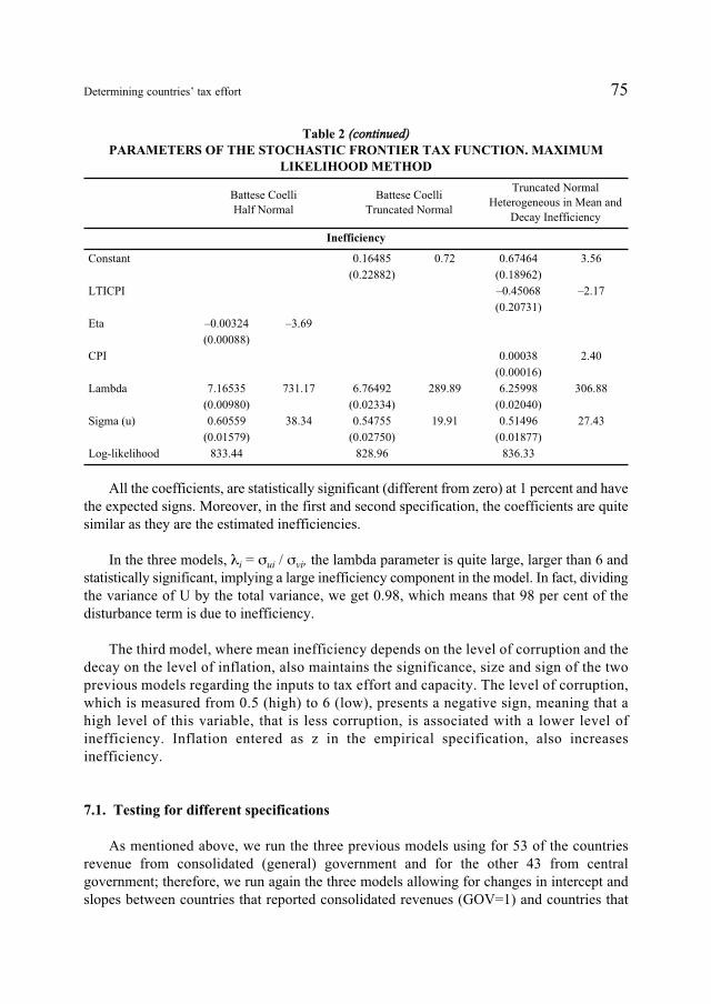
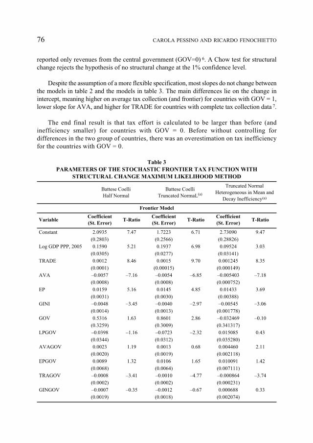
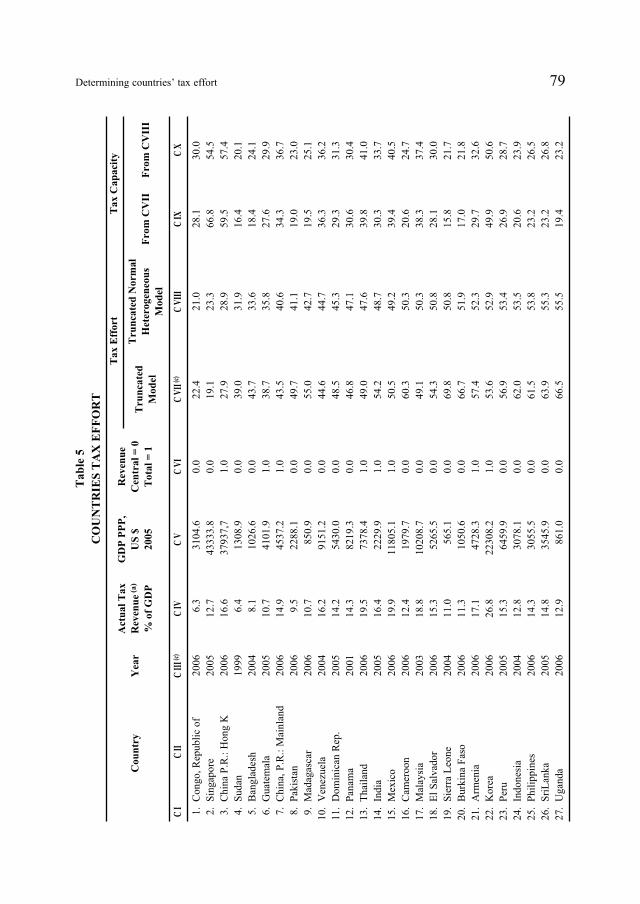
79
CVIII
300
545
574
201
241
299
367
230
251
362
232
X C 313
304
410
337
405
247
374
300
217
218
326
506
287
239
265
268
Capacity
From
CVII
Tax
281
668
595
164
184
IXC 276
343
190
195
363
293
303
306
398
394
206
383
281
158
170
297
499
269
206
232
232
194
From
Normal
Heterogeneous
Model
VIII
210
233
289
319
336
358
406
411
427
447
453
471
476
523
503
508
487
C 503
Truncated
492
508
519
529
534
535
538
553
555
Effort
Tax
Truncated
Model
(c)
224
191
279
390
437
387
435
497
VII
446
490
550
485
468
542
505
603
491
543
698
C 667
574
536
569
620
615
639
665
EFFORT
0 15 TAX
Revenue =
Central
Table = VI 00
00
10
00
00
10
10
00
00
00
00
00
10
10
10
00
00
00
00
00
10
10
00
Total 00
COUNTRIES C 0
000
00
PPP
31046
433338
379377
13089
10266
41019
45372
22881
8509
91512
54300
82193
73784
22299
118051
19797
102087
52655
V US
2005
$ C 5651
10506
47283
64599
30781
35459
8610
GDP
223082
30555
Tax
(a)
Revenue
GDP
Actual IV 63
of C 127
166
64
81
107
149
95
107
162
142
143
195
164
199
124
188
153
110
113
171
268
153
128
143
148
129
Year
2006
2005
2006
1999
2004
2005
2006
2006
2006
III
2004
2006
2005
(c) 2006
2004
2006
2005
2001
2006
2006
C 2003
2006
2006
2005
2004
2006
2005
2006
Kof Republic
Hong
Mainland
Country Rep
II PR C
Singapore
PR Faso
Salvador
Congo Leone
China
Sudan
Bangladesh
Guatemala
China
Pakistan
Madagascar
Venezuela
Dom
inican
Panama
Thailand
India
Cam
eroon
Malaysia
Mexico
El Sierra
Burkina
Armenia
Korea
Peru
Indonesia
Philippines
SriLanka
Uganda
10
11
12
13
14
15
16
17
18
19
20
21
22
23
24
25
C 3 5 26 I 1 2 4 6 7 8 9 27
Determining countriesrsquo tax effort
80
CVIII
378
271
303
258
X C 455
457
357
496
265
431
446
252
439
425
208
429
226
255
334
441
428
463
337
432
257
443
283
Capacity
From
Tax
CVII
IX
From C 319
251
274
240
383
457
320
498
230
389
429
195
438
392
148
421
187
211
326
445
431
456
337
423
228
440
266
Normal
Heterogeneous
Model
VIII
569
590
Truncated 598
590
593
599
602
607
C 608
612
614
615
622
625
635
639
645
653
663
663
666
668
668
678
682
691
692
Effort
Tax
Truncated
Model
(c)
673
637
653
637
710
600
672
604
701
678
639
795
623
678
889
652
781
789
679
658
662
677
667
766
VII
C 693
695
736
))ddeeuu EFFORT
nn 0 i ittnnTAX
Revenue
1= Central =
VI 00
10
00 oocc
COUNTRIES
Total (( C 00
00
10
10
10
00
00
10
00
10
10
00
10
00
00
00
00
10
10
00
10
00
10
00
5Table
PPP
21621
45741
33272
39093
22645
302903
20018
346622
14292
45107
116145
10255
418132
38654
5207
304093
7576
15814
$ V US
GDP C 96013
181451
335987
316561
116603
2005
149137
37186
378866
54981
Tax
(a)
GDP
Actual
Revenue IV
of
C 215
141
179
153
272
274
215
301
161
264
274
155
273
266
132
274
146
166
222
293
285
309
225
293
175
306
196
Year
2004
2005
2006
2006
2003
2006
2004
2006
2001
2006
2006
2006
2005
2006
2003
2006
2006
2006
2006
2005
2003
2005
2004
2006
1999
(c)III
C 2005
2003
Tobago
Country II Republic
C
States
Nicaragua
and
Arab
Egypt
Honduras
Paraguay
Mongolia
Sw
itzerland
Vietnam
Senegal
Jordan
Argentina
Rica
Japan
Mali
United
Bolivia
Ethiopia
Greece
Togo
Cocirctedrsquolvoire
Costa
Trinidad
Canada
Australia
Botswana
Latvia
Syrian
Ireland
Colom
bia
28
29
31
C 30
33
36
37
38
40 I
32
34
35
39
41
42
43
44
45
46
47
48
49
50
51
52
53
54
CAROLA PESSINO AND RICARDO FENOCHIETTO
CVIII
X C 434
591
261
316
433
240
383
491
290
392
221
405
458
439
472
453
470
541
416
450
420
293
433
404
463
461
376
Capacity
From
Tax
CVII
423
577
210
246
427
191
362
502
266
190
387
447
426
463
452
466
IX
541
399
445
382
255
From
C 387
409
392
459
460
362
Normal
Heterogeneous
Model
VIII
695
701
701
709
711
713
729
740
746
755
770
Truncated
C 771
774
782
788
789
797
807
812
816
827
842
845
849
851
858
856
Effort
Tax
ed
Truncatl
Mode (c)
721
718
873
912
896
723
VII
714
813
764
894
C 770
806
792
806
804
791
803
806
848
826
908
967
895
875
858
892
859
))ddeeuu EFFORT
nn 0
nno TAX iitt
o
Revenue
1= Central =
Total
VIcc (( C 10
10
00
00
10
00
10
10
00
10
00
10
10
10
10
10
10
10
10
10
10
00
10
10
10
10
10
5Table
COUNTRIES
PPP
152535
354645
13464
93676
$ V US C 11191
2005
185783
9961
723460
54629
GDP
174523
12334
88067
201515
235185
277679
313232
320417
485259
99768
214372
23216
20491
60316
135714
242488
354187
127972
Tax
(a)
GDP
Revenue
302
414
183
224
308
171
279
363
216
296
170
312
354
343
372
357
374
436
338
Actual IV
of
C 367
347
247
366
343
394
395
323
Year
2006
2005
2005
2004
2006
2005
2005
2006
2005
2006
2006
2006
2006
2002
2006
2006
2006
2006
III 2006
2006
(c) 2006
2002
C 2006
2005
2006
2006
2006
II Guinea
Country
Kingdom
The
Republic
Africa
Zealand
Republic
C Lithuania
Gam
bia
Luxembourg
Iceland
Rom
ania
Albania
Estonia
Slovak
Zambia
Portugal
Germany
New
Kenya
Ghana
South
New
Spain
United
Norway
Bulgaria
Czech
Moldova
Papua
Ukraine
Poland
Slovenia
Netherlands
Russia
55
56
57
58
59
60
61
62
63
64
65
66
67
68
69
70
71
73
75
76
81 I
C 74
72
77
78
79
80
81 Determining countriesrsquo tax effort
CVIII
coshy
X C 291
378
469
403
352
282
490
518
459
360
421
469
446
510
465
and
Capacity
From
Tax inflaction
CVII
280
357
466
394
339
277
490
516
453
348
419
463
439
464
From
C 509
IX
variables
aditional
Normal
Heterogeneous
Model
VIII
858
860
893
921
922
925
926
947
947
951
953
953
958
981
982
Effort
Truncated two
C
include
Tax X
and
Truncated
Model
(c)
890
910
899
942
958
942
927
952
960
984
959
966
972
984
VIII
VII
C 986
column
)) ddeeuunn EFFORT
0 i i 1tt = Trade)
nn = VI
oo
cc TAX
((
Revenue
Central
Total C 00
10
10
10
00
00
10
10
10
10
10
10
10
10
10 and
5 available
GINI
Table
COUNTRIES
PE
were
PPP
109468
59983
V US C 42264
2005
98880
$GDP
349299
177014
319687
345946
320025
86731
138671
309562
281089
331493
94365
AVA
country
(GDP
a of
Tax
(a)
GDP
Revenue variables
Actual IV
of
C 250
325
419
371
324
261
454
491
435
342
402
447
427
501
457
variables
all
of
data
Year
2006
2006
2006
2006
2005
2003
2006
2006
2006
2006
2006
2006
dependent
(c)III
2006
2006
2006 5 C w
hich
Contributions
include
for
IX year
C
and last
Country
VII
the
Social
IIC
show
s
Uruguay
Hungary
Jamaica
Denmark
Finland
Austria
Turkey
Nam
ibia
Belgium
Brazil
Croatia
France
C Italy
Sweden
Belarus
Includes
While
rruption III
C
82
83
84
85
86
87
88
89
90 I
91
92
93
94
95
(a)
(b)
(c) C 96
82 CAROLA PESSINO AND RICARDO FENOCHIETTO
83 Determining countriesrsquo tax effort
Among countries with a low tax effort whose actual tax revenue as percent of GDP is away from their tax capacity we find those with a low level of per capita GDP Some of these countries have a huge level of exemptions (in some cases established by the Constitutions such as the case of Guatemala) and others such as Panama very low rates Therefore in the case of these two countries public choice explains at least a share of the distance between the actual revenue and the maximum level of revenue that these countries could achieve
Exceptions to this other rule are Namibia The Gambia Kenya and Ghana with a very low level of per capita GDP but near their tax capacity (high tax effort) Different reasons explain that these countries have this high level of collection and a low per capita GDP For instance in the case of The Gambia this is explained by the tax collected on the reshyexport trade (people who cross the border from neighbor countries to make purchases)
Another crucial issue that our paper estimates is the impact of inefficiencies on collecting taxes The difference between C VII and C VIII of table 5 shows how tax capacity would increase if corruption and inflation decrease This is particularly the case of Ghana (whose tax effort would increase 203 points ndashfrom 709 to 912ndash if its level of inflation and corruption were similar to the average of the rest of the countries included in our study) Sierra Leone (190) The Gambia (183) Mali (180) Kenya (172) Ethiopia (154) Burkina Faso (148) Togo (136) Cocircted Ivoire (135) Bangladesh (111) Mongolia (111) Nicaragua (104) Cameroon (100) Moldova (81) Pakistan (86) and Jordan (66)
8 Conclusions
The initial step that a country should follow before implementing new taxes or increasing the rate of the existing ones is to analyze its tax effort how far its actual revenue is from their tax capacity If a country is near its tax capacity then changes in the tax system should be oriented to improve its quality or to mildly increase tax rates As well if a country is very near its tax capacity and needs resources to increase its public expenditure it will not be able increase taxes and this country will need to look for another source of financing or renounce to such increase of expenditure
We use a relative method with predictions of tax effort using a comparative analysis of data on these countries That is to say the method determines if a countryrsquo tax capacity is high or low in comparison with tax capacity of the other countries taking into account some characteristics
We use the stochastic frontier tax analysis to determine the tax effort of 96 countries One of the main differences between the development of production frontier and tax frontier is in the results In production frontier the difference between current production and frontier represents the level of inefficiency something that firms do not accomplish In tax frontier the difference between actual revenue and tax capacity includes the existence of technical inefficiencies as well as policy issues (differences in tax legislation for instance in the level of rates) We
84 CAROLA PESSINO AND RICARDO FENOCHIETTO
estimate different specifications of the stochastic frontier using panel data the BatteseshyCoelli half normal truncated normal and this last incorporating heterogeneity
Our study corroborates previous analysis inasmuch as the positive and significant relationship between tax revenue as percent of GDP and the level of development (per capita GDP) trade (imports and exports as percent of GDP) and education (public expenditure on education as percent of GDP) The study also demonstrates the negative relationship between tax revenue as percent of GDP and inflation (CPI) income distribution (GINI coefficient) the ease of tax collection (agricultural sector value added as GDP percent) and corruption
Due to the relationship between tax revenue as percent of GDP (dependent variable) and the independent variables mentioned in the previous paragraph most European countries with high level of per capita GDP and education open economies (particularly since the creation of the customs union) low level of inflation and corruption and strong policies of income distribution have a very high level of tax revenue as percent of GDP and they are near their tax capacity This is something that we expected It is also important to highlight that the high level of their social security contributions is a factor explaining their closeness to tax capacity
Moreover the study demostrates
As some countries with a high per capita GDP have yet capacity to increase their revenue This is the case of Hong Kong Singapore and Korea countries whose per capita GDP (PPP 2005) is higher than US$ 20000 yearly and whose tax effort varies between 191 and 536 percent This does not mean that they have to increase their revenue this is a public choice issue these countries can opt for a low level of revenue and public expenditure
As several countries with low level of revenue are near their maximum level of collection If these countries want to increase their public expenditure (say to increase their social expenditure) they could not increase tax revenue and they should look for other resources This is particularly the case of Ghana Kenya and The Gambia whose per capita GDP (PPP 2005) are lower to US$1350 and their tax effort higher to 70 percent
Some countries that are fare from their tax capacity could increase their revenue significantly by reducing their inefficiencies (particularly the level of corruption)
Acronyms
AVA Value Added of Agriculture CPI Consumption Price Index EP Public Expenditure on Education GDPPPP2005 Gross Domestic Product per capita purchasing power parity constant 2005 TICPI The corruption perception index of Transparency International IMF International Monetary Fund ML Maximum Likelihood WBWDI World Bank World Development Indicators
85 Determining countriesrsquo tax effort
Notas
1 For a more comprehensive analysis of the stochastic frontier production function see Batesse et al (2005) Chapter 9
2 For more details see Caudill Ford and Gropper (1995) and Wang and Schmidt (2002)
3 We do not include in the analysis countries in which revenue from hydrocarbons represent more than 30 percent of total tax revenue because a significant portion of revenue from hydrocarbons is classified as nontax revenue (such as royalties or permits to explore) Therefore tax revenue in these countries is usually low and non tax revenue high and this affects comparison For instance in Kuwait in 2006 while tax revenue was equivalent to 09 percent of GDP nontax revenue (property income) was 476 percent of GDP
4 There were not available data for the 96 countries included in the sample of other variables such as ldquotime to prepare and pay taxes (hours)rdquo that can also be proxy of the ease of tax collection
5 We run the three Battese Coelli specifications shown in Section 5 but we also tried different functional form specifications Greene (2008) found consistent with other researchers that estimates of technical efficiency are quite robust to distributional assumptions to the choice of fixed or random effects and to methodology Bayesian vs classical but estimates of technical are quite sensitive to the crucial assumption of time invariance In our case the estimates were robust to different functional forms and also to the assumption of time invariance More research remains to be done in studying specifications with true random and fixed effects
6 The variables LPGOV AVAGOV EPGOV TRAGOV GINGOV are respectively the original variables Log GDP PPP2005 AVA EP TRADE and GINI multiplied (interacted) by the dummy GOV
8 The chi squared statistic for the joint test of the hypothesis that the coefficients of the Dummy GOV and the five interaction variables equal zero at the 95 level is 567 918 and 367 respectively in each of the models of table III The Chi Squared with six restrictions is 1295 clearly lower than any of those statistics hence rejecting the hypothesis of no structural change
8 C VII shows tax effort taking into account five dependent variables GDP GINI coefficient trade agricultural sector and public expenditure on education C VIII also shows tax capacity but taking into account two additional independent variables those that represent inefficiency inflation and corruption
9 Salinas and Salinas (2007) using a (i) frontier approach to estimate production frontier (defined as the maximum technically attainable level of production and the associated relative efficiency levels) in a sample of 22 OECD countries during the period 1980ndash2000 and different corruption indicators showed that this variable negatively affects the efficiency levels at which these economies perform
Referencias
Agbeyegbe T Stotsky J and WoldeMariam A (2004) ldquoTrade Liberalization Exchange Rate Changes and Tax Revenue in SubshySaharan Africardquo Working Paper No 04178 International Monetary Fund Washington DC
Aigner DJ Lovell Knox CA and Schmidt P ldquoFormulation and Estimation of Stochastic Frontier Production Function Modelsrdquo Journal of Econometrics Vol 6 1977 21shy37
Alfirman L (2003) ldquoEstimating Stochastic Frontier Tax Potential Can Indonesian Local Governments Increase Tax Revenues Under Decentralizationrdquo Department of Economics University of Colorado at Boulder Colorado Working Paper No 03shy19
Battese GE (1992) ldquoFrontier Production Functions and Technical Efficiencies A Survey of Empirical Applications in Agricultural Economicsrdquo Agricultural Economics Vol 7
86 CAROLA PESSINO AND RICARDO FENOCHIETTO
Battese G and Coelli T (1992) ldquoFrontier Production Functions Technical Efficiency and Panel Data With Application to Paddy Farmers in Indiardquo Journal of Productivity Analysis 3 153shy169
Battese GE Coelli T OrsquoDonnell CJ Timothy J and Prasada DS (2005) ldquoAn Introduction to Efficiency and Productivity Analysisrdquo Second Edition 2005 Springer Verlag
Caudill S Ford J and Gropper D (1995) ldquoFrontier Estimation and Firm Specific Inefficiency Measures in the Presence of Heteroscedasticityrdquo Journal of Business and Economic Statistics 13 105shy111
Coelli T (1992) ldquoA Computer Program for Frontier Production Function Estimationrdquo Economics Letters Vol 39 29shy32
Coelli T Rao D OrsquoDonnell C and Battese G (2005) ldquoAn Introduction to Efficiency and Productivity Analysisrdquo 2nd Edition Springer ISBN 978shy0shy387shy24266shy8
Combes JshyL and SaadishySedik T (2006) ldquoHow Does Trade Openness Influence Budget Deficits in Developing Countriesrdquo Working Paper 0603 International Monetary Fund Washington DC
Coondo D Majumder A Mukherjee R and Neogi C (2003) ldquoTax Performance and Taxable Capacity Analysis for Selected States of Indiardquo Journal of Public Finance and Public Choice Vol 21 25shy46
Davoodi H and Grigorian D (2007) ldquoTax Potential vs Tax Effort A CrossshyCountry Analysis of Armeniarsquos Stubbornly Low Tax Collectionrdquo WP07106
Esteller A (2003) ldquoLa eficiencia en la administracioacuten de los tributos cedidos un anaacutelisis explicativordquo Papeles de economiacutea espantildeola 320shy334
Greene WH (1990) ldquoA Gamma Distributed Stochastic Frontier Modelrdquo Journal of Econometrics 46 pp 141shy163
Greene WH (2008) ldquoThe Econometric Approach to Efficiency Analysisrdquo In The Measurement of Productive Efficiency and Productivity Growth Fried HO Knox Lovell CA and Schmidt SS (editors) Oxford University Press Oxford Chapter 2 92shy250
Gupta A (2007) ldquoDeterminants of Tax Revenue Efforts in Developing Countriesrdquo IMF Working Paper
Jondrow J Materov I and Schmidt P (1982) ldquoOn the Estimation of Technical Inefficiency in the Stochastic Frontier Production Function Modelrdquo Journal of Econometrics 233shy238
Keen M and Simone A (2004) ldquoTax Policy in Developing Countries Some Lessons from the 1990s and Some Challenges Aheadrdquo in Helping Countries Develop The Role of Fiscal Policy ed by Sanjeev Gupta Benedict Clements and Gabriela Inchauste International Monetary Fund Washington DC
Kumbhakar S and K Lovell (2000) ldquoStochastic Frontier Analysis Cambridge University Pressrdquo Cambridge
Leuthold J (1991) ldquoTax Shares in Developing Economies A Panel Studyrdquo Journal of Development Economics 35 173shy85
Lotz J and Morrs E (1967) ldquoMeasuring lsquoTax Effortrsquo in Developing Countriesrdquo Staff Papers Vol 14 No 3 November 1967 478shy499 International Monetary Fund Washington DC
Pitt M and Lee L (1981) ldquoThe Measurement and Sources of Technical Inefficiency in the Indonesian Weaving Industryrdquo Journal of Development Economics 9 43shy64
87 Determining countriesrsquo tax effort
SalinasshyJimenez M and SalinasshyJimenez J (2007) Corruption efficiency and productivity in OECD countries Instituto de Estudios Fiscales Universidad de Extremadura Spain
Stevenson R (1980) ldquoLikelihood Functions for Generalized Stochastic Frontier Estimationrdquo Journal of Econometrics 13 58shy66
Stotsky J and WoldeMariam A (1997) ldquoTax Effort in SubshySaharan Africardquo Working Paper 97107 International Monetary Fund Washington DC
Tanzi V (1987) ldquoQuantitative Characteristics of the Tax Systems of Developing Countriesrdquo in the theory of Taxation for Developing Countries edited by David New and Nicholas Stern New York Oxford University
Tanzi V and Zee HH (2000) ldquoTax policy for Emerging Markets Developing Countriesrdquo International Monetary Fund Washington DC Working Paper0035 March 2000
Tanzi V (1987) ldquoQuantitative Characteristics of the Tax Systems of Developing Countriesrdquo in David Newbery and Nicholas Stern (eds) The Theory of Taxation in Developing Countries Oxford University Press
Tanzi V and H Davoodi (1997) ldquoCorruption Public Investment and Growthrdquo Working Paper 97139 International Monetary Fund Washington DC
Varsano R Pessoa A Costa da Silva N Rodrigues Alfonso J e Ramundo J (1998) ldquoUma Anaacutelise da Carga Tributaacuteria do Brasilrdquo Texto para Discussatildeo nordm 583 Rio de Janeiro IPEA
Wang H and P Schmidt (2002) ldquoOne Step and Two Step Estimation of the Effects of Exogenous Variables on Technical Efficiency Levelsrdquo Journal of Productivity Analysis 18 129shy144
Resumen
El presente estudio desarrolla un modelo para determinar el esfuerzo y la capacidad tributaria de 96 paiacuteses y las principales variables de las cuales dicho esfuerzo y capacidad dependen Los reshysultados obtenidos permiten determinar queacute paiacuteses se encuentran cerca de su maacuteximo nivel de reshycaudacioacuten y cuaacuteles no Nuestro trabajo corrobora estudios previos al encontrar una relacioacuten positishyva y significativa entre el nivel de recaudacioacuten medido como porcentaje del PBI y el nivel de desarrollo (PBI per caacutepita) la apertura econoacutemica (importaciones y exportaciones como porcentashyje del PBI) y el nivel de educacioacuten de los habitantes de un paiacutes (gasto puacuteblico en educacioacuten como porcentaje del PBI) Asimismo demuestra la relacioacuten negativa y significativa entre dicho nivel de recaudacioacuten con la inflacioacuten (medida a traveacutes de la variacioacuten en el iacutendice de precios al consumishydor) la distribucioacuten del ingreso (medida a traveacutes del coeficiente de GINI) la facilidad de un paiacutes para recaudar impuestos (medida a traveacutes del valor del producto agropecuario como porcentaje del PBI) y la corrupcioacuten
Palabras clave esfuerzo tributario capacidad tributaria recaudacioacuten tributaria frontera tributaria esshytocaacutestica ineficiencia
Clasificacioacuten JEL C23 C51 H2 H21
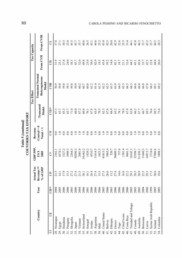
80
CVIII
378
271
303
258
X C 455
457
357
496
265
431
446
252
439
425
208
429
226
255
334
441
428
463
337
432
257
443
283
Capacity
From
Tax
CVII
IX
From C 319
251
274
240
383
457
320
498
230
389
429
195
438
392
148
421
187
211
326
445
431
456
337
423
228
440
266
Normal
Heterogeneous
Model
VIII
569
590
Truncated 598
590
593
599
602
607
C 608
612
614
615
622
625
635
639
645
653
663
663
666
668
668
678
682
691
692
Effort
Tax
Truncated
Model
(c)
673
637
653
637
710
600
672
604
701
678
639
795
623
678
889
652
781
789
679
658
662
677
667
766
VII
C 693
695
736
))ddeeuu EFFORT
nn 0 i ittnnTAX
Revenue
1= Central =
VI 00
10
00 oocc
COUNTRIES
Total (( C 00
00
10
10
10
00
00
10
00
10
10
00
10
00
00
00
00
10
10
00
10
00
10
00
5Table
PPP
21621
45741
33272
39093
22645
302903
20018
346622
14292
45107
116145
10255
418132
38654
5207
304093
7576
15814
$ V US
GDP C 96013
181451
335987
316561
116603
2005
149137
37186
378866
54981
Tax
(a)
GDP
Actual
Revenue IV
of
C 215
141
179
153
272
274
215
301
161
264
274
155
273
266
132
274
146
166
222
293
285
309
225
293
175
306
196
Year
2004
2005
2006
2006
2003
2006
2004
2006
2001
2006
2006
2006
2005
2006
2003
2006
2006
2006
2006
2005
2003
2005
2004
2006
1999
(c)III
C 2005
2003
Tobago
Country II Republic
C
States
Nicaragua
and
Arab
Egypt
Honduras
Paraguay
Mongolia
Sw
itzerland
Vietnam
Senegal
Jordan
Argentina
Rica
Japan
Mali
United
Bolivia
Ethiopia
Greece
Togo
Cocirctedrsquolvoire
Costa
Trinidad
Canada
Australia
Botswana
Latvia
Syrian
Ireland
Colom
bia
28
29
31
C 30
33
36
37
38
40 I
32
34
35
39
41
42
43
44
45
46
47
48
49
50
51
52
53
54
CAROLA PESSINO AND RICARDO FENOCHIETTO
CVIII
X C 434
591
261
316
433
240
383
491
290
392
221
405
458
439
472
453
470
541
416
450
420
293
433
404
463
461
376
Capacity
From
Tax
CVII
423
577
210
246
427
191
362
502
266
190
387
447
426
463
452
466
IX
541
399
445
382
255
From
C 387
409
392
459
460
362
Normal
Heterogeneous
Model
VIII
695
701
701
709
711
713
729
740
746
755
770
Truncated
C 771
774
782
788
789
797
807
812
816
827
842
845
849
851
858
856
Effort
Tax
ed
Truncatl
Mode (c)
721
718
873
912
896
723
VII
714
813
764
894
C 770
806
792
806
804
791
803
806
848
826
908
967
895
875
858
892
859
))ddeeuu EFFORT
nn 0
nno TAX iitt
o
Revenue
1= Central =
Total
VIcc (( C 10
10
00
00
10
00
10
10
00
10
00
10
10
10
10
10
10
10
10
10
10
00
10
10
10
10
10
5Table
COUNTRIES
PPP
152535
354645
13464
93676
$ V US C 11191
2005
185783
9961
723460
54629
GDP
174523
12334
88067
201515
235185
277679
313232
320417
485259
99768
214372
23216
20491
60316
135714
242488
354187
127972
Tax
(a)
GDP
Revenue
302
414
183
224
308
171
279
363
216
296
170
312
354
343
372
357
374
436
338
Actual IV
of
C 367
347
247
366
343
394
395
323
Year
2006
2005
2005
2004
2006
2005
2005
2006
2005
2006
2006
2006
2006
2002
2006
2006
2006
2006
III 2006
2006
(c) 2006
2002
C 2006
2005
2006
2006
2006
II Guinea
Country
Kingdom
The
Republic
Africa
Zealand
Republic
C Lithuania
Gam
bia
Luxembourg
Iceland
Rom
ania
Albania
Estonia
Slovak
Zambia
Portugal
Germany
New
Kenya
Ghana
South
New
Spain
United
Norway
Bulgaria
Czech
Moldova
Papua
Ukraine
Poland
Slovenia
Netherlands
Russia
55
56
57
58
59
60
61
62
63
64
65
66
67
68
69
70
71
73
75
76
81 I
C 74
72
77
78
79
80
81 Determining countriesrsquo tax effort
CVIII
coshy
X C 291
378
469
403
352
282
490
518
459
360
421
469
446
510
465
and
Capacity
From
Tax inflaction
CVII
280
357
466
394
339
277
490
516
453
348
419
463
439
464
From
C 509
IX
variables
aditional
Normal
Heterogeneous
Model
VIII
858
860
893
921
922
925
926
947
947
951
953
953
958
981
982
Effort
Truncated two
C
include
Tax X
and
Truncated
Model
(c)
890
910
899
942
958
942
927
952
960
984
959
966
972
984
VIII
VII
C 986
column
)) ddeeuunn EFFORT
0 i i 1tt = Trade)
nn = VI
oo
cc TAX
((
Revenue
Central
Total C 00
10
10
10
00
00
10
10
10
10
10
10
10
10
10 and
5 available
GINI
Table
COUNTRIES
PE
were
PPP
109468
59983
V US C 42264
2005
98880
$GDP
349299
177014
319687
345946
320025
86731
138671
309562
281089
331493
94365
AVA
country
(GDP
a of
Tax
(a)
GDP
Revenue variables
Actual IV
of
C 250
325
419
371
324
261
454
491
435
342
402
447
427
501
457
variables
all
of
data
Year
2006
2006
2006
2006
2005
2003
2006
2006
2006
2006
2006
2006
dependent
(c)III
2006
2006
2006 5 C w
hich
Contributions
include
for
IX year
C
and last
Country
VII
the
Social
IIC
show
s
Uruguay
Hungary
Jamaica
Denmark
Finland
Austria
Turkey
Nam
ibia
Belgium
Brazil
Croatia
France
C Italy
Sweden
Belarus
Includes
While
rruption III
C
82
83
84
85
86
87
88
89
90 I
91
92
93
94
95
(a)
(b)
(c) C 96
82 CAROLA PESSINO AND RICARDO FENOCHIETTO
83 Determining countriesrsquo tax effort
Among countries with a low tax effort whose actual tax revenue as percent of GDP is away from their tax capacity we find those with a low level of per capita GDP Some of these countries have a huge level of exemptions (in some cases established by the Constitutions such as the case of Guatemala) and others such as Panama very low rates Therefore in the case of these two countries public choice explains at least a share of the distance between the actual revenue and the maximum level of revenue that these countries could achieve
Exceptions to this other rule are Namibia The Gambia Kenya and Ghana with a very low level of per capita GDP but near their tax capacity (high tax effort) Different reasons explain that these countries have this high level of collection and a low per capita GDP For instance in the case of The Gambia this is explained by the tax collected on the reshyexport trade (people who cross the border from neighbor countries to make purchases)
Another crucial issue that our paper estimates is the impact of inefficiencies on collecting taxes The difference between C VII and C VIII of table 5 shows how tax capacity would increase if corruption and inflation decrease This is particularly the case of Ghana (whose tax effort would increase 203 points ndashfrom 709 to 912ndash if its level of inflation and corruption were similar to the average of the rest of the countries included in our study) Sierra Leone (190) The Gambia (183) Mali (180) Kenya (172) Ethiopia (154) Burkina Faso (148) Togo (136) Cocircted Ivoire (135) Bangladesh (111) Mongolia (111) Nicaragua (104) Cameroon (100) Moldova (81) Pakistan (86) and Jordan (66)
8 Conclusions
The initial step that a country should follow before implementing new taxes or increasing the rate of the existing ones is to analyze its tax effort how far its actual revenue is from their tax capacity If a country is near its tax capacity then changes in the tax system should be oriented to improve its quality or to mildly increase tax rates As well if a country is very near its tax capacity and needs resources to increase its public expenditure it will not be able increase taxes and this country will need to look for another source of financing or renounce to such increase of expenditure
We use a relative method with predictions of tax effort using a comparative analysis of data on these countries That is to say the method determines if a countryrsquo tax capacity is high or low in comparison with tax capacity of the other countries taking into account some characteristics
We use the stochastic frontier tax analysis to determine the tax effort of 96 countries One of the main differences between the development of production frontier and tax frontier is in the results In production frontier the difference between current production and frontier represents the level of inefficiency something that firms do not accomplish In tax frontier the difference between actual revenue and tax capacity includes the existence of technical inefficiencies as well as policy issues (differences in tax legislation for instance in the level of rates) We
84 CAROLA PESSINO AND RICARDO FENOCHIETTO
estimate different specifications of the stochastic frontier using panel data the BatteseshyCoelli half normal truncated normal and this last incorporating heterogeneity
Our study corroborates previous analysis inasmuch as the positive and significant relationship between tax revenue as percent of GDP and the level of development (per capita GDP) trade (imports and exports as percent of GDP) and education (public expenditure on education as percent of GDP) The study also demonstrates the negative relationship between tax revenue as percent of GDP and inflation (CPI) income distribution (GINI coefficient) the ease of tax collection (agricultural sector value added as GDP percent) and corruption
Due to the relationship between tax revenue as percent of GDP (dependent variable) and the independent variables mentioned in the previous paragraph most European countries with high level of per capita GDP and education open economies (particularly since the creation of the customs union) low level of inflation and corruption and strong policies of income distribution have a very high level of tax revenue as percent of GDP and they are near their tax capacity This is something that we expected It is also important to highlight that the high level of their social security contributions is a factor explaining their closeness to tax capacity
Moreover the study demostrates
As some countries with a high per capita GDP have yet capacity to increase their revenue This is the case of Hong Kong Singapore and Korea countries whose per capita GDP (PPP 2005) is higher than US$ 20000 yearly and whose tax effort varies between 191 and 536 percent This does not mean that they have to increase their revenue this is a public choice issue these countries can opt for a low level of revenue and public expenditure
As several countries with low level of revenue are near their maximum level of collection If these countries want to increase their public expenditure (say to increase their social expenditure) they could not increase tax revenue and they should look for other resources This is particularly the case of Ghana Kenya and The Gambia whose per capita GDP (PPP 2005) are lower to US$1350 and their tax effort higher to 70 percent
Some countries that are fare from their tax capacity could increase their revenue significantly by reducing their inefficiencies (particularly the level of corruption)
Acronyms
AVA Value Added of Agriculture CPI Consumption Price Index EP Public Expenditure on Education GDPPPP2005 Gross Domestic Product per capita purchasing power parity constant 2005 TICPI The corruption perception index of Transparency International IMF International Monetary Fund ML Maximum Likelihood WBWDI World Bank World Development Indicators
85 Determining countriesrsquo tax effort
Notas
1 For a more comprehensive analysis of the stochastic frontier production function see Batesse et al (2005) Chapter 9
2 For more details see Caudill Ford and Gropper (1995) and Wang and Schmidt (2002)
3 We do not include in the analysis countries in which revenue from hydrocarbons represent more than 30 percent of total tax revenue because a significant portion of revenue from hydrocarbons is classified as nontax revenue (such as royalties or permits to explore) Therefore tax revenue in these countries is usually low and non tax revenue high and this affects comparison For instance in Kuwait in 2006 while tax revenue was equivalent to 09 percent of GDP nontax revenue (property income) was 476 percent of GDP
4 There were not available data for the 96 countries included in the sample of other variables such as ldquotime to prepare and pay taxes (hours)rdquo that can also be proxy of the ease of tax collection
5 We run the three Battese Coelli specifications shown in Section 5 but we also tried different functional form specifications Greene (2008) found consistent with other researchers that estimates of technical efficiency are quite robust to distributional assumptions to the choice of fixed or random effects and to methodology Bayesian vs classical but estimates of technical are quite sensitive to the crucial assumption of time invariance In our case the estimates were robust to different functional forms and also to the assumption of time invariance More research remains to be done in studying specifications with true random and fixed effects
6 The variables LPGOV AVAGOV EPGOV TRAGOV GINGOV are respectively the original variables Log GDP PPP2005 AVA EP TRADE and GINI multiplied (interacted) by the dummy GOV
8 The chi squared statistic for the joint test of the hypothesis that the coefficients of the Dummy GOV and the five interaction variables equal zero at the 95 level is 567 918 and 367 respectively in each of the models of table III The Chi Squared with six restrictions is 1295 clearly lower than any of those statistics hence rejecting the hypothesis of no structural change
8 C VII shows tax effort taking into account five dependent variables GDP GINI coefficient trade agricultural sector and public expenditure on education C VIII also shows tax capacity but taking into account two additional independent variables those that represent inefficiency inflation and corruption
9 Salinas and Salinas (2007) using a (i) frontier approach to estimate production frontier (defined as the maximum technically attainable level of production and the associated relative efficiency levels) in a sample of 22 OECD countries during the period 1980ndash2000 and different corruption indicators showed that this variable negatively affects the efficiency levels at which these economies perform
Referencias
Agbeyegbe T Stotsky J and WoldeMariam A (2004) ldquoTrade Liberalization Exchange Rate Changes and Tax Revenue in SubshySaharan Africardquo Working Paper No 04178 International Monetary Fund Washington DC
Aigner DJ Lovell Knox CA and Schmidt P ldquoFormulation and Estimation of Stochastic Frontier Production Function Modelsrdquo Journal of Econometrics Vol 6 1977 21shy37
Alfirman L (2003) ldquoEstimating Stochastic Frontier Tax Potential Can Indonesian Local Governments Increase Tax Revenues Under Decentralizationrdquo Department of Economics University of Colorado at Boulder Colorado Working Paper No 03shy19
Battese GE (1992) ldquoFrontier Production Functions and Technical Efficiencies A Survey of Empirical Applications in Agricultural Economicsrdquo Agricultural Economics Vol 7
86 CAROLA PESSINO AND RICARDO FENOCHIETTO
Battese G and Coelli T (1992) ldquoFrontier Production Functions Technical Efficiency and Panel Data With Application to Paddy Farmers in Indiardquo Journal of Productivity Analysis 3 153shy169
Battese GE Coelli T OrsquoDonnell CJ Timothy J and Prasada DS (2005) ldquoAn Introduction to Efficiency and Productivity Analysisrdquo Second Edition 2005 Springer Verlag
Caudill S Ford J and Gropper D (1995) ldquoFrontier Estimation and Firm Specific Inefficiency Measures in the Presence of Heteroscedasticityrdquo Journal of Business and Economic Statistics 13 105shy111
Coelli T (1992) ldquoA Computer Program for Frontier Production Function Estimationrdquo Economics Letters Vol 39 29shy32
Coelli T Rao D OrsquoDonnell C and Battese G (2005) ldquoAn Introduction to Efficiency and Productivity Analysisrdquo 2nd Edition Springer ISBN 978shy0shy387shy24266shy8
Combes JshyL and SaadishySedik T (2006) ldquoHow Does Trade Openness Influence Budget Deficits in Developing Countriesrdquo Working Paper 0603 International Monetary Fund Washington DC
Coondo D Majumder A Mukherjee R and Neogi C (2003) ldquoTax Performance and Taxable Capacity Analysis for Selected States of Indiardquo Journal of Public Finance and Public Choice Vol 21 25shy46
Davoodi H and Grigorian D (2007) ldquoTax Potential vs Tax Effort A CrossshyCountry Analysis of Armeniarsquos Stubbornly Low Tax Collectionrdquo WP07106
Esteller A (2003) ldquoLa eficiencia en la administracioacuten de los tributos cedidos un anaacutelisis explicativordquo Papeles de economiacutea espantildeola 320shy334
Greene WH (1990) ldquoA Gamma Distributed Stochastic Frontier Modelrdquo Journal of Econometrics 46 pp 141shy163
Greene WH (2008) ldquoThe Econometric Approach to Efficiency Analysisrdquo In The Measurement of Productive Efficiency and Productivity Growth Fried HO Knox Lovell CA and Schmidt SS (editors) Oxford University Press Oxford Chapter 2 92shy250
Gupta A (2007) ldquoDeterminants of Tax Revenue Efforts in Developing Countriesrdquo IMF Working Paper
Jondrow J Materov I and Schmidt P (1982) ldquoOn the Estimation of Technical Inefficiency in the Stochastic Frontier Production Function Modelrdquo Journal of Econometrics 233shy238
Keen M and Simone A (2004) ldquoTax Policy in Developing Countries Some Lessons from the 1990s and Some Challenges Aheadrdquo in Helping Countries Develop The Role of Fiscal Policy ed by Sanjeev Gupta Benedict Clements and Gabriela Inchauste International Monetary Fund Washington DC
Kumbhakar S and K Lovell (2000) ldquoStochastic Frontier Analysis Cambridge University Pressrdquo Cambridge
Leuthold J (1991) ldquoTax Shares in Developing Economies A Panel Studyrdquo Journal of Development Economics 35 173shy85
Lotz J and Morrs E (1967) ldquoMeasuring lsquoTax Effortrsquo in Developing Countriesrdquo Staff Papers Vol 14 No 3 November 1967 478shy499 International Monetary Fund Washington DC
Pitt M and Lee L (1981) ldquoThe Measurement and Sources of Technical Inefficiency in the Indonesian Weaving Industryrdquo Journal of Development Economics 9 43shy64
87 Determining countriesrsquo tax effort
SalinasshyJimenez M and SalinasshyJimenez J (2007) Corruption efficiency and productivity in OECD countries Instituto de Estudios Fiscales Universidad de Extremadura Spain
Stevenson R (1980) ldquoLikelihood Functions for Generalized Stochastic Frontier Estimationrdquo Journal of Econometrics 13 58shy66
Stotsky J and WoldeMariam A (1997) ldquoTax Effort in SubshySaharan Africardquo Working Paper 97107 International Monetary Fund Washington DC
Tanzi V (1987) ldquoQuantitative Characteristics of the Tax Systems of Developing Countriesrdquo in the theory of Taxation for Developing Countries edited by David New and Nicholas Stern New York Oxford University
Tanzi V and Zee HH (2000) ldquoTax policy for Emerging Markets Developing Countriesrdquo International Monetary Fund Washington DC Working Paper0035 March 2000
Tanzi V (1987) ldquoQuantitative Characteristics of the Tax Systems of Developing Countriesrdquo in David Newbery and Nicholas Stern (eds) The Theory of Taxation in Developing Countries Oxford University Press
Tanzi V and H Davoodi (1997) ldquoCorruption Public Investment and Growthrdquo Working Paper 97139 International Monetary Fund Washington DC
Varsano R Pessoa A Costa da Silva N Rodrigues Alfonso J e Ramundo J (1998) ldquoUma Anaacutelise da Carga Tributaacuteria do Brasilrdquo Texto para Discussatildeo nordm 583 Rio de Janeiro IPEA
Wang H and P Schmidt (2002) ldquoOne Step and Two Step Estimation of the Effects of Exogenous Variables on Technical Efficiency Levelsrdquo Journal of Productivity Analysis 18 129shy144
Resumen
El presente estudio desarrolla un modelo para determinar el esfuerzo y la capacidad tributaria de 96 paiacuteses y las principales variables de las cuales dicho esfuerzo y capacidad dependen Los reshysultados obtenidos permiten determinar queacute paiacuteses se encuentran cerca de su maacuteximo nivel de reshycaudacioacuten y cuaacuteles no Nuestro trabajo corrobora estudios previos al encontrar una relacioacuten positishyva y significativa entre el nivel de recaudacioacuten medido como porcentaje del PBI y el nivel de desarrollo (PBI per caacutepita) la apertura econoacutemica (importaciones y exportaciones como porcentashyje del PBI) y el nivel de educacioacuten de los habitantes de un paiacutes (gasto puacuteblico en educacioacuten como porcentaje del PBI) Asimismo demuestra la relacioacuten negativa y significativa entre dicho nivel de recaudacioacuten con la inflacioacuten (medida a traveacutes de la variacioacuten en el iacutendice de precios al consumishydor) la distribucioacuten del ingreso (medida a traveacutes del coeficiente de GINI) la facilidad de un paiacutes para recaudar impuestos (medida a traveacutes del valor del producto agropecuario como porcentaje del PBI) y la corrupcioacuten
Palabras clave esfuerzo tributario capacidad tributaria recaudacioacuten tributaria frontera tributaria esshytocaacutestica ineficiencia
Clasificacioacuten JEL C23 C51 H2 H21

CVIII
coshy
X C 291
378
469
403
352
282
490
518
459
360
421
469
446
510
465
and
Capacity
From
Tax inflaction
CVII
280
357
466
394
339
277
490
516
453
348
419
463
439
464
From
C 509
IX
variables
aditional
Normal
Heterogeneous
Model
VIII
858
860
893
921
922
925
926
947
947
951
953
953
958
981
982
Effort
Truncated two
C
include
Tax X
and
Truncated
Model
(c)
890
910
899
942
958
942
927
952
960
984
959
966
972
984
VIII
VII
C 986
column
)) ddeeuunn EFFORT
0 i i 1tt = Trade)
nn = VI
oo
cc TAX
((
Revenue
Central
Total C 00
10
10
10
00
00
10
10
10
10
10
10
10
10
10 and
5 available
GINI
Table
COUNTRIES
PE
were
PPP
109468
59983
V US C 42264
2005
98880
$GDP
349299
177014
319687
345946
320025
86731
138671
309562
281089
331493
94365
AVA
country
(GDP
a of
Tax
(a)
GDP
Revenue variables
Actual IV
of
C 250
325
419
371
324
261
454
491
435
342
402
447
427
501
457
variables
all
of
data
Year
2006
2006
2006
2006
2005
2003
2006
2006
2006
2006
2006
2006
dependent
(c)III
2006
2006
2006 5 C w
hich
Contributions
include
for
IX year
C
and last
Country
VII
the
Social
IIC
show
s
Uruguay
Hungary
Jamaica
Denmark
Finland
Austria
Turkey
Nam
ibia
Belgium
Brazil
Croatia
France
C Italy
Sweden
Belarus
Includes
While
rruption III
C
82
83
84
85
86
87
88
89
90 I
91
92
93
94
95
(a)
(b)
(c) C 96
82 CAROLA PESSINO AND RICARDO FENOCHIETTO
83 Determining countriesrsquo tax effort
Among countries with a low tax effort whose actual tax revenue as percent of GDP is away from their tax capacity we find those with a low level of per capita GDP Some of these countries have a huge level of exemptions (in some cases established by the Constitutions such as the case of Guatemala) and others such as Panama very low rates Therefore in the case of these two countries public choice explains at least a share of the distance between the actual revenue and the maximum level of revenue that these countries could achieve
Exceptions to this other rule are Namibia The Gambia Kenya and Ghana with a very low level of per capita GDP but near their tax capacity (high tax effort) Different reasons explain that these countries have this high level of collection and a low per capita GDP For instance in the case of The Gambia this is explained by the tax collected on the reshyexport trade (people who cross the border from neighbor countries to make purchases)
Another crucial issue that our paper estimates is the impact of inefficiencies on collecting taxes The difference between C VII and C VIII of table 5 shows how tax capacity would increase if corruption and inflation decrease This is particularly the case of Ghana (whose tax effort would increase 203 points ndashfrom 709 to 912ndash if its level of inflation and corruption were similar to the average of the rest of the countries included in our study) Sierra Leone (190) The Gambia (183) Mali (180) Kenya (172) Ethiopia (154) Burkina Faso (148) Togo (136) Cocircted Ivoire (135) Bangladesh (111) Mongolia (111) Nicaragua (104) Cameroon (100) Moldova (81) Pakistan (86) and Jordan (66)
8 Conclusions
The initial step that a country should follow before implementing new taxes or increasing the rate of the existing ones is to analyze its tax effort how far its actual revenue is from their tax capacity If a country is near its tax capacity then changes in the tax system should be oriented to improve its quality or to mildly increase tax rates As well if a country is very near its tax capacity and needs resources to increase its public expenditure it will not be able increase taxes and this country will need to look for another source of financing or renounce to such increase of expenditure
We use a relative method with predictions of tax effort using a comparative analysis of data on these countries That is to say the method determines if a countryrsquo tax capacity is high or low in comparison with tax capacity of the other countries taking into account some characteristics
We use the stochastic frontier tax analysis to determine the tax effort of 96 countries One of the main differences between the development of production frontier and tax frontier is in the results In production frontier the difference between current production and frontier represents the level of inefficiency something that firms do not accomplish In tax frontier the difference between actual revenue and tax capacity includes the existence of technical inefficiencies as well as policy issues (differences in tax legislation for instance in the level of rates) We
84 CAROLA PESSINO AND RICARDO FENOCHIETTO
estimate different specifications of the stochastic frontier using panel data the BatteseshyCoelli half normal truncated normal and this last incorporating heterogeneity
Our study corroborates previous analysis inasmuch as the positive and significant relationship between tax revenue as percent of GDP and the level of development (per capita GDP) trade (imports and exports as percent of GDP) and education (public expenditure on education as percent of GDP) The study also demonstrates the negative relationship between tax revenue as percent of GDP and inflation (CPI) income distribution (GINI coefficient) the ease of tax collection (agricultural sector value added as GDP percent) and corruption
Due to the relationship between tax revenue as percent of GDP (dependent variable) and the independent variables mentioned in the previous paragraph most European countries with high level of per capita GDP and education open economies (particularly since the creation of the customs union) low level of inflation and corruption and strong policies of income distribution have a very high level of tax revenue as percent of GDP and they are near their tax capacity This is something that we expected It is also important to highlight that the high level of their social security contributions is a factor explaining their closeness to tax capacity
Moreover the study demostrates
As some countries with a high per capita GDP have yet capacity to increase their revenue This is the case of Hong Kong Singapore and Korea countries whose per capita GDP (PPP 2005) is higher than US$ 20000 yearly and whose tax effort varies between 191 and 536 percent This does not mean that they have to increase their revenue this is a public choice issue these countries can opt for a low level of revenue and public expenditure
As several countries with low level of revenue are near their maximum level of collection If these countries want to increase their public expenditure (say to increase their social expenditure) they could not increase tax revenue and they should look for other resources This is particularly the case of Ghana Kenya and The Gambia whose per capita GDP (PPP 2005) are lower to US$1350 and their tax effort higher to 70 percent
Some countries that are fare from their tax capacity could increase their revenue significantly by reducing their inefficiencies (particularly the level of corruption)
Acronyms
AVA Value Added of Agriculture CPI Consumption Price Index EP Public Expenditure on Education GDPPPP2005 Gross Domestic Product per capita purchasing power parity constant 2005 TICPI The corruption perception index of Transparency International IMF International Monetary Fund ML Maximum Likelihood WBWDI World Bank World Development Indicators
85 Determining countriesrsquo tax effort
Notas
1 For a more comprehensive analysis of the stochastic frontier production function see Batesse et al (2005) Chapter 9
2 For more details see Caudill Ford and Gropper (1995) and Wang and Schmidt (2002)
3 We do not include in the analysis countries in which revenue from hydrocarbons represent more than 30 percent of total tax revenue because a significant portion of revenue from hydrocarbons is classified as nontax revenue (such as royalties or permits to explore) Therefore tax revenue in these countries is usually low and non tax revenue high and this affects comparison For instance in Kuwait in 2006 while tax revenue was equivalent to 09 percent of GDP nontax revenue (property income) was 476 percent of GDP
4 There were not available data for the 96 countries included in the sample of other variables such as ldquotime to prepare and pay taxes (hours)rdquo that can also be proxy of the ease of tax collection
5 We run the three Battese Coelli specifications shown in Section 5 but we also tried different functional form specifications Greene (2008) found consistent with other researchers that estimates of technical efficiency are quite robust to distributional assumptions to the choice of fixed or random effects and to methodology Bayesian vs classical but estimates of technical are quite sensitive to the crucial assumption of time invariance In our case the estimates were robust to different functional forms and also to the assumption of time invariance More research remains to be done in studying specifications with true random and fixed effects
6 The variables LPGOV AVAGOV EPGOV TRAGOV GINGOV are respectively the original variables Log GDP PPP2005 AVA EP TRADE and GINI multiplied (interacted) by the dummy GOV
8 The chi squared statistic for the joint test of the hypothesis that the coefficients of the Dummy GOV and the five interaction variables equal zero at the 95 level is 567 918 and 367 respectively in each of the models of table III The Chi Squared with six restrictions is 1295 clearly lower than any of those statistics hence rejecting the hypothesis of no structural change
8 C VII shows tax effort taking into account five dependent variables GDP GINI coefficient trade agricultural sector and public expenditure on education C VIII also shows tax capacity but taking into account two additional independent variables those that represent inefficiency inflation and corruption
9 Salinas and Salinas (2007) using a (i) frontier approach to estimate production frontier (defined as the maximum technically attainable level of production and the associated relative efficiency levels) in a sample of 22 OECD countries during the period 1980ndash2000 and different corruption indicators showed that this variable negatively affects the efficiency levels at which these economies perform
Referencias
Agbeyegbe T Stotsky J and WoldeMariam A (2004) ldquoTrade Liberalization Exchange Rate Changes and Tax Revenue in SubshySaharan Africardquo Working Paper No 04178 International Monetary Fund Washington DC
Aigner DJ Lovell Knox CA and Schmidt P ldquoFormulation and Estimation of Stochastic Frontier Production Function Modelsrdquo Journal of Econometrics Vol 6 1977 21shy37
Alfirman L (2003) ldquoEstimating Stochastic Frontier Tax Potential Can Indonesian Local Governments Increase Tax Revenues Under Decentralizationrdquo Department of Economics University of Colorado at Boulder Colorado Working Paper No 03shy19
Battese GE (1992) ldquoFrontier Production Functions and Technical Efficiencies A Survey of Empirical Applications in Agricultural Economicsrdquo Agricultural Economics Vol 7
86 CAROLA PESSINO AND RICARDO FENOCHIETTO
Battese G and Coelli T (1992) ldquoFrontier Production Functions Technical Efficiency and Panel Data With Application to Paddy Farmers in Indiardquo Journal of Productivity Analysis 3 153shy169
Battese GE Coelli T OrsquoDonnell CJ Timothy J and Prasada DS (2005) ldquoAn Introduction to Efficiency and Productivity Analysisrdquo Second Edition 2005 Springer Verlag
Caudill S Ford J and Gropper D (1995) ldquoFrontier Estimation and Firm Specific Inefficiency Measures in the Presence of Heteroscedasticityrdquo Journal of Business and Economic Statistics 13 105shy111
Coelli T (1992) ldquoA Computer Program for Frontier Production Function Estimationrdquo Economics Letters Vol 39 29shy32
Coelli T Rao D OrsquoDonnell C and Battese G (2005) ldquoAn Introduction to Efficiency and Productivity Analysisrdquo 2nd Edition Springer ISBN 978shy0shy387shy24266shy8
Combes JshyL and SaadishySedik T (2006) ldquoHow Does Trade Openness Influence Budget Deficits in Developing Countriesrdquo Working Paper 0603 International Monetary Fund Washington DC
Coondo D Majumder A Mukherjee R and Neogi C (2003) ldquoTax Performance and Taxable Capacity Analysis for Selected States of Indiardquo Journal of Public Finance and Public Choice Vol 21 25shy46
Davoodi H and Grigorian D (2007) ldquoTax Potential vs Tax Effort A CrossshyCountry Analysis of Armeniarsquos Stubbornly Low Tax Collectionrdquo WP07106
Esteller A (2003) ldquoLa eficiencia en la administracioacuten de los tributos cedidos un anaacutelisis explicativordquo Papeles de economiacutea espantildeola 320shy334
Greene WH (1990) ldquoA Gamma Distributed Stochastic Frontier Modelrdquo Journal of Econometrics 46 pp 141shy163
Greene WH (2008) ldquoThe Econometric Approach to Efficiency Analysisrdquo In The Measurement of Productive Efficiency and Productivity Growth Fried HO Knox Lovell CA and Schmidt SS (editors) Oxford University Press Oxford Chapter 2 92shy250
Gupta A (2007) ldquoDeterminants of Tax Revenue Efforts in Developing Countriesrdquo IMF Working Paper
Jondrow J Materov I and Schmidt P (1982) ldquoOn the Estimation of Technical Inefficiency in the Stochastic Frontier Production Function Modelrdquo Journal of Econometrics 233shy238
Keen M and Simone A (2004) ldquoTax Policy in Developing Countries Some Lessons from the 1990s and Some Challenges Aheadrdquo in Helping Countries Develop The Role of Fiscal Policy ed by Sanjeev Gupta Benedict Clements and Gabriela Inchauste International Monetary Fund Washington DC
Kumbhakar S and K Lovell (2000) ldquoStochastic Frontier Analysis Cambridge University Pressrdquo Cambridge
Leuthold J (1991) ldquoTax Shares in Developing Economies A Panel Studyrdquo Journal of Development Economics 35 173shy85
Lotz J and Morrs E (1967) ldquoMeasuring lsquoTax Effortrsquo in Developing Countriesrdquo Staff Papers Vol 14 No 3 November 1967 478shy499 International Monetary Fund Washington DC
Pitt M and Lee L (1981) ldquoThe Measurement and Sources of Technical Inefficiency in the Indonesian Weaving Industryrdquo Journal of Development Economics 9 43shy64
87 Determining countriesrsquo tax effort
SalinasshyJimenez M and SalinasshyJimenez J (2007) Corruption efficiency and productivity in OECD countries Instituto de Estudios Fiscales Universidad de Extremadura Spain
Stevenson R (1980) ldquoLikelihood Functions for Generalized Stochastic Frontier Estimationrdquo Journal of Econometrics 13 58shy66
Stotsky J and WoldeMariam A (1997) ldquoTax Effort in SubshySaharan Africardquo Working Paper 97107 International Monetary Fund Washington DC
Tanzi V (1987) ldquoQuantitative Characteristics of the Tax Systems of Developing Countriesrdquo in the theory of Taxation for Developing Countries edited by David New and Nicholas Stern New York Oxford University
Tanzi V and Zee HH (2000) ldquoTax policy for Emerging Markets Developing Countriesrdquo International Monetary Fund Washington DC Working Paper0035 March 2000
Tanzi V (1987) ldquoQuantitative Characteristics of the Tax Systems of Developing Countriesrdquo in David Newbery and Nicholas Stern (eds) The Theory of Taxation in Developing Countries Oxford University Press
Tanzi V and H Davoodi (1997) ldquoCorruption Public Investment and Growthrdquo Working Paper 97139 International Monetary Fund Washington DC
Varsano R Pessoa A Costa da Silva N Rodrigues Alfonso J e Ramundo J (1998) ldquoUma Anaacutelise da Carga Tributaacuteria do Brasilrdquo Texto para Discussatildeo nordm 583 Rio de Janeiro IPEA
Wang H and P Schmidt (2002) ldquoOne Step and Two Step Estimation of the Effects of Exogenous Variables on Technical Efficiency Levelsrdquo Journal of Productivity Analysis 18 129shy144
Resumen
El presente estudio desarrolla un modelo para determinar el esfuerzo y la capacidad tributaria de 96 paiacuteses y las principales variables de las cuales dicho esfuerzo y capacidad dependen Los reshysultados obtenidos permiten determinar queacute paiacuteses se encuentran cerca de su maacuteximo nivel de reshycaudacioacuten y cuaacuteles no Nuestro trabajo corrobora estudios previos al encontrar una relacioacuten positishyva y significativa entre el nivel de recaudacioacuten medido como porcentaje del PBI y el nivel de desarrollo (PBI per caacutepita) la apertura econoacutemica (importaciones y exportaciones como porcentashyje del PBI) y el nivel de educacioacuten de los habitantes de un paiacutes (gasto puacuteblico en educacioacuten como porcentaje del PBI) Asimismo demuestra la relacioacuten negativa y significativa entre dicho nivel de recaudacioacuten con la inflacioacuten (medida a traveacutes de la variacioacuten en el iacutendice de precios al consumishydor) la distribucioacuten del ingreso (medida a traveacutes del coeficiente de GINI) la facilidad de un paiacutes para recaudar impuestos (medida a traveacutes del valor del producto agropecuario como porcentaje del PBI) y la corrupcioacuten
Palabras clave esfuerzo tributario capacidad tributaria recaudacioacuten tributaria frontera tributaria esshytocaacutestica ineficiencia
Clasificacioacuten JEL C23 C51 H2 H21
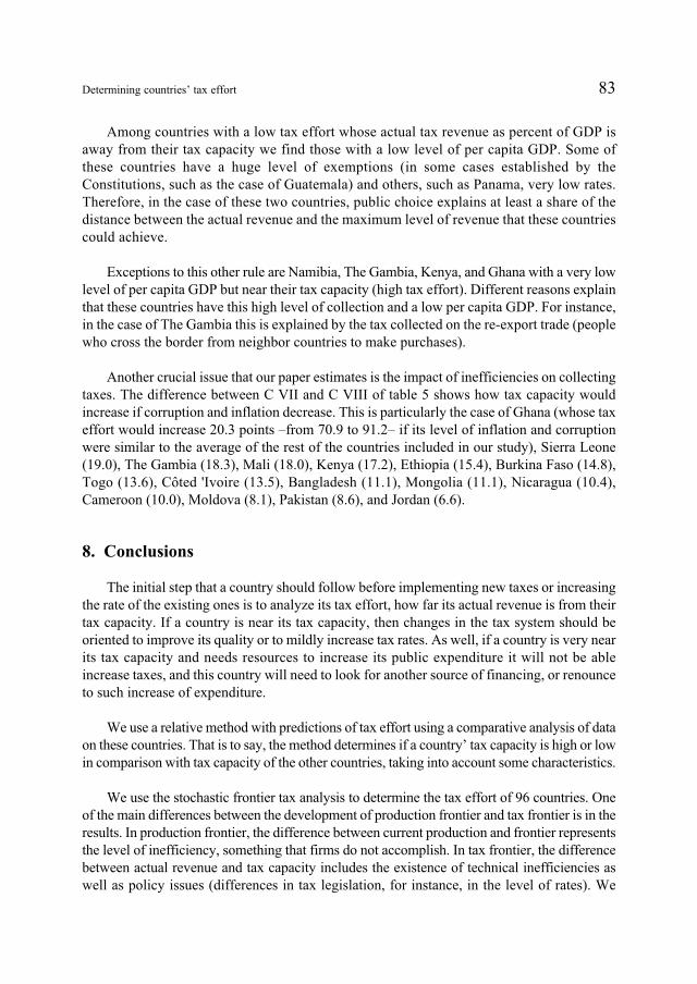
