Seediscussions,stats,andauthorprofilesforthispublicationat:https://www.researchgate.net/publication/231743703

Ellipticandtriangularinstabilitiesinrotatingcylinders

ARTICLEinJOURNALOFFLUIDMECHANICS·FEBRUARY2003

ImpactFactor:2.38·DOI:10.1017/S0022112002002999

CITATIONS

54

READS

24

3AUTHORS:

ChristopheEloy

EcoleCentraleMarseille

71PUBLICATIONS820CITATIONS

SEEPROFILE

PatriceLeGal

Aix-MarseilleUniversité

154PUBLICATIONS1,723CITATIONS

SEEPROFILE

StephaneLeDizes

FrenchNationalCentreforScientificResea…

150PUBLICATIONS1,338CITATIONS

SEEPROFILE

Availablefrom:PatriceLeGal

Retrievedon:04February2016

J. Fluid Mech. (2003), vol. 476, pp. 357–388. c© 2003 Cambridge University Press

DOI: 10.1017/S0022112002002999 Printed in the United Kingdom

357

Elliptic and triangular instabilities inrotating cylinders

By C H R I S T O P H E E L O Y, P A T R I C E L E G A LAND S T E P H A N E L E D I Z E S

Institut de Recherche sur les Phenomenes Hors Equilibre, CNRS UMR 6594, UniversitesAix-Marseille I et II, 49, rue Joliot Curie – BP 146, 13384 Marseille Cedex 13, France

(Received 28 January 2002 and in revised form 4 September 2002)

In this article, the multipolar vortex instability of the flow in a finite cylinder isaddressed. The experimental study uses a rotating elastic deformable tube filledwith water which is elliptically or triangularly deformed by two or three rollers.The experimental control parameters are the cylinder aspect ratio and the Reynoldsnumber based on the angular frequency.

For Reynolds numbers close to threshold, different instability modes are visualizedusing anisotropic particles, according to the value of the aspect ratio. These modesare compared with those predicted by an asymptotic stability theory in the limitof small deformations and large Reynolds numbers. A very good agreement isobtained which confirms the instability mechanism; for both elliptic and triangularconfigurations, the instability is due to the resonance of two normal modes (Kelvinmodes) of the underlying rotating flow with the deformation field. At least fourdifferent elliptic instability modes, including combinations of Kelvin modes withazimuthal wavenumbers m = 0 and m = 2 and Kelvin modes m = 1 and m = 3 arevisualized. Two different triangular instability modes which are a combination ofKelvin modes m = −1 and m = 2 and a combination of Kelvin modes m = 0 andm = 3 are also evidenced.

The nonlinear dynamics of a particular elliptic instability mode, which correspondsto the combination of two stationary Kelvin modes m = −1 and m = 1, is examinedin more detail using particle image velocimetry (PIV). The dynamics of the phase andamplitude of the instability mode is shown to be predicted well by the weakly nonlinearanalysis for moderate Reynolds numbers. For larger Reynolds number, a secondaryinstability is observed. Below a Reynolds number threshold, the amplitude of thisinstability mode saturates and its frequency is shown to agree with the predictionsof Kerswell (1999). Above this threshold, a more complex dynamic develops which isonly sustained during a finite time. Eventually, the two-dimensional stationary ellipticflow is reestablished and the destabilization process starts again.

1. IntroductionStrong vorticity filaments have been evidenced in turbulent flows experimentally

(Cadot, Douady & Couder 1995) and numerically (see Jimenez & Wray 1998 andreferences therein). The discovery of these coherent structures has renewed the interestin vortex dynamics, as it was outlined by Pullin & Saffman (1998) in their recent review.The formation of these filaments was related to shear flow instabilities by Passot etal. (1995). However, several issues concerning the dynamics of these structures in

358 C. Eloy, P. Le Gal and S. Le Dizes

turbulent flows and their breakdown are still open. In recent numerical simulations oftransition to turbulence of gravity waves, Arendt, Fritts & Andreassen (1998) showedthe presence of Kelvin modes on vortex filaments which cannot be explained by theusual vorticity tilting and stretching arguments. One aim in this study is to providea possible mechanism for the apparition of these modes in terms of an instability ofvorticity filaments caused by the surrounding turbulent flow: namely the multipolarinstability.

A model commonly used for vorticity filaments in turbulence is the Burgers (1948)vortex. This axisymmetric vortex, of Gaussian vorticity profile, is a stationary solutionof the Navier–Stokes equations for which viscous diffusion is exactly compensated byaxial stretching. Moffatt, Kida & Ohkitani (1994) (see also Ting & Tung 1965) showedthat an external strain field would induce a first-order correction to the Burgers modelwhich deforms the streamlines inside the core from circles to ellipses. Using numericalsimulations of turbulent flows (Kida & Ohkitani 1992), Moffatt et al. (1994) alsoshowed that the energy dissipation field of vortex filaments is reproduced remarkablywell by this elliptically distorted Burgers vortex. Prochazka & Pullin (1998) latershowed the bi-dimensional stability of Moffatt et al.’s (1994) solution but Eloy & LeDizes (1999) established its sensitivity to the tri-dimensional elliptic instability. Thisinstability could explain the appearance of Kelvin modes on the filament since theyare its natural modes.

The elliptic instability was (re)discovered by Pierrehumbert (1986) and Bayly (1986)in the context of parallel shear flows as a secondary instability of Kelvin–Helmoltzvortices (see also Bayly, Holm & Lifschitz 1996 and references therein). However,the first stability studies of vortices with elliptic streamlines are due to Gledzeret al. (1975), Moore & Saffman (1975) and Tsai & Widnall (1976). In a recentreview, Kerswell (2002) stressed how the elliptic instability has been discovered inthe 1970s and then rediscovered in 1986 in a different context (see this review for acomprehensive bibliography on the subject). The physical mechanism of this instabilitycan be understood as follows. First, we should assume the existence of Kelvinmodes which are neutral normal modes characterized by their axial wavenumber,azimuthal wavenumber and frequency [k, m, ω]. Then, the elliptic deformation of thestreamlines should be interpreted as an intrinsic mode of characteristics [k, m, ω] =[0,±2, 0]. The instability mechanism is a triadic resonance of this intrinsic mode andtwo Kelvin modes of the same axial wavenumber, same frequency and azimuthalwavenumbers differing by 2. Moore & Saffman (1975) showed that combinationsof stationary (ω = 0) and helical (m = ±1) Kelvin modes are always resonant andunstable. However, as pointed out by Billant, Brancher & Chomaz (1999), the ellipticinstability is not limited to these particular combinations. Indeed, Eloy & Le Dizes(2001) analysed all the possible resonances for the Rankine vortex and demonstratedthat a combination of a bulging Kelvin mode (m = 0) and a splitting mode (m = 2)could appear spontaneously.

The mechanism of the elliptic instability has been generalized to flows with higherazimuthal symmetry by Le Dizes & Eloy (1999) and Eloy & Le Dizes (2001). Itappears that a vortex subject to an n-fold multipolar strain field is always unstableif n = 2, 3 or 4, giving rise to what has been called the multipolar instability. Forsymmetry of higher degree, the flow is unstable only if the external strain field issufficiently strong.

The experimental study of the elliptic instability began with the pioneering workof Gledzer et al. (1974, 1975). They used a rigid cylinder of elliptic cross-section (anellipsoid in their 1974 paper) filled with water seeded with reflective particles. This

Elliptic and triangular instabilities in rotating cylinders 359

container was rotated until solid-body rotation was reached and then it was sharplystopped. During the transient decay of the flow, the streamlines are elliptical and thismay lead to the elliptic instability. Later Chernous’ko (1978) used the same set-upand studied the wavelength of the instability as a function of two control parametersof the experiment: the eccentricity of the elliptic cylinder and its aspect ratio. Hisresults agree remarkably well with the theoretical prediction of Gledzer & Ponomarev(1992) for undulating modes (a combination of two stationary helical Kelvin modes).Nevertheless, this set-up has two main inconveniences: first, the instability developson a transiently decaying flow (thus during a limited time); and a competitivecentrifugal instability appears near the wall. To avoid the shortcomings of Gledzer’sexperiment, Malkus (1989) and Malkus & Waleffe (1991) used a deformable elasticcylinder rotated at constant angular speed. Using a belt or two rollers, this cylindercould be deformed elliptically, such that the axes of the ellipse were kept still in thelaboratory frame. This experiment produced a stationary elliptic basic flow on whichthe undulating modes already reported by Gledzer et al. (1975) were observed. Thisexperiment showed the intermittent character of the instability at high rotation rate.Indeed, the amplitude of the instability modes was not observed to saturate in theregimes studied; a cycle of instability growth, mode breakdown and relaminarizationtook place, as will be described in detail.

Besides the physics of small-scale turbulent structures, another important field wherethe elliptical instability could have a considerable interest is astro- and geophysics.Indeed, the tidal effects experienced by rotating planets or other astrophysical objectscreated by the proximity of others are of great interest. In particular, we can easilyimagine that the Earth molten iron outer core is deformed by the gravitational strainsof the Moon and Sun and therefore is subject to an elliptical instability. Kerswell(1994) estimated that the global loss due to friction and ohmic dissipation has thesame order of magnitude as the growth rates of unstable modes in rotating spheroids.Thus, the energy gained by the elliptic instability could very well be part (withconvective and precessional instabilities) of the energy source required to sustain thegeodynamo effect. For instance, Kerswell & Malkus (1998) interpreted Io’s magneticsignature by the distortion of its inner molten core due to the gravitational fieldof Jupiter. The first experiments on rotating flows inside ellipsoids were due toGledzer et al. (1974). Later, a series of experiments and calculations by Aldridge et al.(1997) and Seyed-Mahmoud, Henderson & Aldridge (2000) also showed the existenceof such an instability inside a rotating deformable shell which models the Earth’sinterior with its inner solid core. Note that, in this particular geometry, the math-ematical existence of inertial waves deserves its own particular mathematical analysis(Rieutord & Valdetarro 1997).

In addition, the elliptic instability was observed in open flow configurations suchas counter-rotating (Leweke & Williamson 1998a) and co-rotating vortex filaments(Meunier & Leweke 2001, 2002). It was also identified as a mechanism for secondaryinstability in parallel shear flows (Bayly, Orszag & Herbert 1988) and wakes (Leweke& Williamson 1998b).

In the present study, we investigate the elliptic instability and its generalizationto the ‘triangular’ instability both experimentally and theoretically. Our work can beviewed as a continuation and a generalization of earlier studies by Malkus and co-workers (Malkus 1989; Malkus & Waleffe 1991). It is also a more detailed account ofthe results briefly reported in Eloy, Le Gal & Le Dizes (2000). The paper is organizedas follows. In § 2, the set-up and the experimental procedure are presented. In § 3,the theoretical linear stability of this flow is addressed using asymptotic analysis in

360 C. Eloy, P. Le Gal and S. Le Dizes

Roller Plastic transparent cylinder

R

HΩ

Roller

Transparent lid

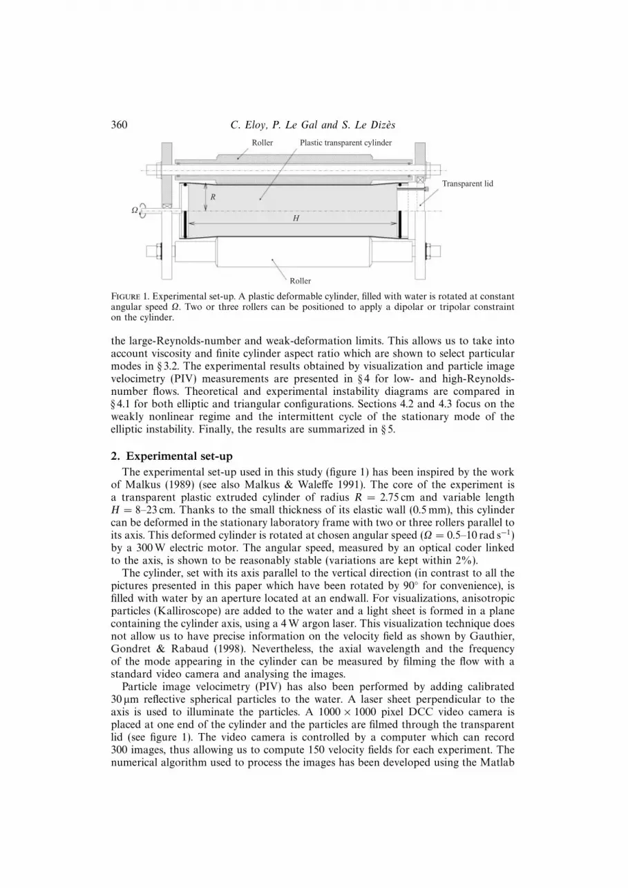
Figure 1. Experimental set-up. A plastic deformable cylinder, filled with water is rotated at constantangular speed Ω. Two or three rollers can be positioned to apply a dipolar or tripolar constrainton the cylinder.

the large-Reynolds-number and weak-deformation limits. This allows us to take intoaccount viscosity and finite cylinder aspect ratio which are shown to select particularmodes in § 3.2. The experimental results obtained by visualization and particle imagevelocimetry (PIV) measurements are presented in § 4 for low- and high-Reynolds-number flows. Theoretical and experimental instability diagrams are compared in§ 4.1 for both elliptic and triangular configurations. Sections 4.2 and 4.3 focus on theweakly nonlinear regime and the intermittent cycle of the stationary mode of theelliptic instability. Finally, the results are summarized in § 5.

2. Experimental set-upThe experimental set-up used in this study (figure 1) has been inspired by the work

of Malkus (1989) (see also Malkus & Waleffe 1991). The core of the experiment isa transparent plastic extruded cylinder of radius R = 2.75 cm and variable lengthH = 8–23 cm. Thanks to the small thickness of its elastic wall (0.5 mm), this cylindercan be deformed in the stationary laboratory frame with two or three rollers parallel toits axis. This deformed cylinder is rotated at chosen angular speed (Ω = 0.5–10 rad s−1)by a 300 W electric motor. The angular speed, measured by an optical coder linkedto the axis, is shown to be reasonably stable (variations are kept within 2%).

The cylinder, set with its axis parallel to the vertical direction (in contrast to all thepictures presented in this paper which have been rotated by 90 for convenience), isfilled with water by an aperture located at an endwall. For visualizations, anisotropicparticles (Kalliroscope) are added to the water and a light sheet is formed in a planecontaining the cylinder axis, using a 4 W argon laser. This visualization technique doesnot allow us to have precise information on the velocity field as shown by Gauthier,Gondret & Rabaud (1998). Nevertheless, the axial wavelength and the frequencyof the mode appearing in the cylinder can be measured by filming the flow with astandard video camera and analysing the images.

Particle image velocimetry (PIV) has also been performed by adding calibrated30 µm reflective spherical particles to the water. A laser sheet perpendicular to theaxis is used to illuminate the particles. A 1000× 1000 pixel DCC video camera isplaced at one end of the cylinder and the particles are filmed through the transparentlid (see figure 1). The video camera is controlled by a computer which can record300 images, thus allowing us to compute 150 velocity fields for each experiment. Thenumerical algorithm used to process the images has been developed using the Matlab

Elliptic and triangular instabilities in rotating cylinders 361

software by Meunier & Leweke (2001, 2002) and can therefore be run on a commonPC computer. Typically, it takes about 4 h to compute 150 velocity fields (containing60× 60 velocity vectors each).

To limit experimental artefacts, attention is paid to several crucial points. First, theorthogonality of the endwalls and the cylinder axis is checked with good precisionto avoid precession type instability. The mechanical properties of the elastic cylinderbeing modified by its ageing, care is also taken by using cylinders for fairly shortperiods of time and by avoiding important constraints. Finally, the presence of bubblesin the flow is prevented by waterproofing the whole cylinder.

The two dimensionless control parameters of this experiment are:

Re =ΩR2

ν: Reynolds number, (2.1a)

H

R: aspect ratio, (2.1b)

which can be varied in the limits Re = 300–8000 and H/R = 3–8.2. From a practicalpoint of view, two sets of rollers have been used allowing the aspect ratio to be variedin the ranges H/R = 3–4 and 7–8.2. The third control parameter of the experimentwould be the strength of the constraint imposed by the rollers on the cylinder, butthe variation of this parameter has not been considered in the present study.

In all the experiments presented in this paper, the same protocol has been followed:(i) The two or three rollers used to deformed the cylinder are positioned;(ii) When the fluid is assured to be at rest (after at least 10 min), the cylinder is

suddenly rotated at constant angular speed;(iii) During all the experiment, the roller position and the cylinder speed are kept

constant.The linear stability of the flow produced by this set-up is addressed theoretically inthe next section. Experimental results are presented in § 4 and discussed in § 5.

3. Linear stability study3.1. Inviscid analysis

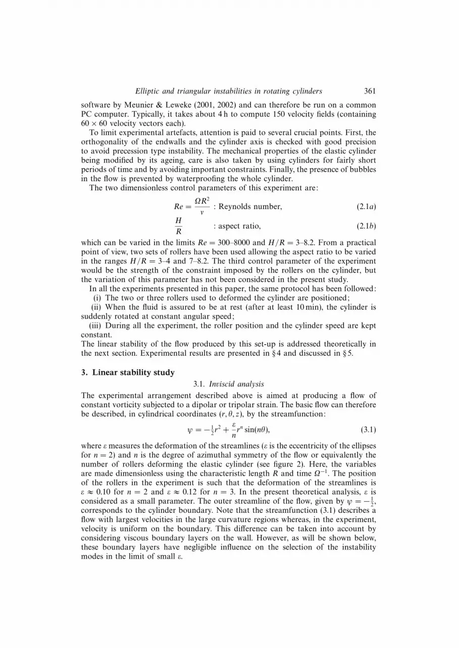
The experimental arrangement described above is aimed at producing a flow ofconstant vorticity subjected to a dipolar or tripolar strain. The basic flow can thereforebe described, in cylindrical coordinates (r, θ, z), by the streamfunction:

ψ = − 12r2 +

ε

nrn sin(nθ), (3.1)

where ε measures the deformation of the streamlines (ε is the eccentricity of the ellipsesfor n = 2) and n is the degree of azimuthal symmetry of the flow or equivalently thenumber of rollers deforming the elastic cylinder (see figure 2). Here, the variablesare made dimensionless using the characteristic length R and time Ω−1. The positionof the rollers in the experiment is such that the deformation of the streamlines isε ≈ 0.10 for n = 2 and ε ≈ 0.12 for n = 3. In the present theoretical analysis, ε isconsidered as a small parameter. The outer streamline of the flow, given by ψ = − 1

2,

corresponds to the cylinder boundary. Note that the streamfunction (3.1) describes aflow with largest velocities in the large curvature regions whereas, in the experiment,velocity is uniform on the boundary. This difference can be taken into account byconsidering viscous boundary layers on the wall. However, as will be shown below,these boundary layers have negligible influence on the selection of the instabilitymodes in the limit of small ε.

362 C. Eloy, P. Le Gal and S. Le Dizes

(a) (b)

Figure 2. Streamlines of the basic flow given by (3.1). The parameters are ε = 0.25 and: (a) n = 2;(b) n = 3. The flow is rotating counterclockwise.

0 2 4 6 8 10

0

1

2

3

4

–3

–2

–1

ω

k

1 2 3 4

1 2 3 4

Figure 3. Dispersion relation of the Kelvin modes inside a cylinder. Eight branches are shown inthe (k, ω)-plane for m = −1 (solid lines) and m = 2 (dashed lines).

The stability of the basic flow (3.1) has been studied using a local approach byLe Dizes & Eloy (1999). It has been shown to be unstable in the limit of vanishingviscosity with the dimensionless growth rate σ = 9

16ε for n = 2 and σ = 49

32ε for n = 3.

The stability of the same flow embedded in an irrotational flow was considered byglobal methods in Eloy & Le Dizes (2001). The selection of the instability modes byboth finite size and viscous effects was analysed in details. Here, the basic flow (3.1) isembedded in a cylinder which makes the stability results slightly different. However,since the method of analysis is the same as in Eloy & Le Dizes (2001), we shall notdetail the calculation but only outline its different stages in the following.

For purely axisymmetric flow (ε = 0), normal Kelvin modes (Kelvin 1880) can besuperimposed linearly to the basic flow. Their velocity field can be written as:

v(r, θ, z, t) = U (r) ei(kz+mθ−ωt) + c.c., (3.2)

where k, m and ω are the axial wavenumber, the azimuthal wavenumber and thefrequency and U (r) is given in the Appendix (the notation c.c. simply refers to thecomplex conjugate). These Kelvin modes are marginally stable for an axisymmetricand inviscid flow. Upon imposing the boundary condition on the cylinder wall (inr = 1), a dispersion relation connecting the different wavenumbers can be found(see the Appendix). This dispersion relation is illustrated in figure 3. For a chosenazimuthal wavenumber m, there is an infinity of branches in the (k, ω)-plane whichaccumulate in ω = m in the limit of small k and in ω = m ± 2 in the limit ofinfinite k.

Elliptic and triangular instabilities in rotating cylinders 363

Elliptic Triangular

i (−1, 1, i) (0, 2, i) (1, 3, i) (−1, 2, i) (0, 3, i) (1, 4, i)

1 1.58 2.33 3.04 3.67 5.18 6.612 3.29 4.12 4.92 7.18 8.81 10.363 5.06 5.92 6.75 10.72 12.40 14.01

Table 1. Table of the axial wavenumbers k for a few principal modes. These wavenumbers can beslightly modified in a cylinder of finite aspect ratio and in the presence of viscosity.

In the limit of small deformation ε, Kelvin modes still exist. As mentioned in theintroduction, two Kelvin modes can resonate with the basic flow if they have samek, same ω and have azimuthal wavenumbers m1 and m2 such that m2 − m1 = n. Forinstance, in figure 3, the crossing points of the dispersion relations for m1 = −1 andm2 = 2 then correspond to points of resonance for a triangular deformation of thevortex (n = 3). A stability study similar to that of Eloy & Le Dizes (2001) shows thatall Kelvin mode resonances are unstable. However, crossing points of branches withthe same label (see figure 3) are significantly more amplified than the others. Theseparticular combinations of Kelvin modes are called principal modes and are denoted

(m1, m2, i), (3.3)

hereinafter, where m1 and m2 are the azimuthal wavenumbers of the two Kelvinmodes and i is the common label of the dispersion relation branches. Note that iis an increasing function of the axial wavenumber k. Table 1 gives the value of thefirst axial wavenumbers k as a function of i for a few principal modes. Owing tothe asymptotic symmetry of the dispersion relation, the frequency of principal modessatisfies ω ≈ 1

2(m1 +m2). In the following, only the principal modes will be taken into

account in the analysis since their inviscid growth rate is about 100 times larger thanthat of other combinations of resonant Kelvin modes.

For an infinite cylinder and in the limit of vanishing viscosity, the growth rate ofthe different principal modes can be found by similar techniques to those detailed inEloy & Le Dizes (2001). The results for the inviscid growth rate σi are summarizedin figure 4. For elliptic deformation (n = 2), the maximum inviscid growth rate isσi = 9

16ε. It is reached in the limit of large k either when the azimuthal wavenumber

m1 tends to infinity for a fixed label i or when i tends to infinity for fixed m1.However, the instability is not very selective in the elliptic case, since the inviscidgrowth rates of the different principal modes are all within 10% of the maximum.For the triangular deformation (n = 3), the inviscid growth rate is maximum in thelimit of large azimuthal wavenumber m1, for fixed label i. This maximum is σi = 49

32ε.

Note that, in the triangular case, the selection of the different principal modes is muchmore efficient. As for the Rankine vortex (Eloy & Le Dizes 2001), the local maximumgrowth rate found in Le Dizes & Eloy (1999) is recovered in the limit of large k forelliptic deformation and in the limit of large m1 and k for triangular deformation.

3.2. Effects of viscosity and aspect ratio

As seen above, in the absence of viscosity and for infinite cylinder, the maximumgrowth rate is reached for infinite k. Under these approximations, the selected modeswould have infinite axial wavenumber for n = 2 and infinite axial and azimuthalwavenumber for n = 3. Of course, this result cannot hold when viscosity is added

364 C. Eloy, P. Le Gal and S. Le Dizes

0 5 10 15 20 25 30 35

0.57

0.56

0.55

0.54

0.53

0.52

0.51

(a)

σiε

0 10 20 30 40 50k

1.6

1.4

1.2

1.0

0.8

0.6

(b)

σiε

Figure 4. Inviscid growth rate σi for (a) n = 2 and (b) n = 3 as a function of the axial wavenumberk. The growth rate of principal modes (m1, m1 + n, i) are presented with: +, m1 = −1; , m1 = 0;, m1 = 1; 4, m1 = 10 and ©, m1 = 20. The solid line corresponds to the first principal modes(m1, m1 + n, 1) for −1 6 m1 6 39. The asymptotic values of the inviscid growth rate are pictured bydotted lines: (a) σi = 9

16ε; (b) σi = 49

8π2 ε and σi = 4932ε.

since it tends to damp the modes with the largest wavenumbers. In this section,boundary viscous effects and volume viscous effects are first taken into account inthe stability analysis. Then, the effect of the finite aspect ratio of the cylinder will beanalysed. As will be shown, these two effects can efficiently select particular modes. Asimilar study, in a different context, has also been carried out by Racz & Scott (2001a).

As described above, the inviscid (dimensionless) growth rate of principal modesis σi = O(ε). The distinguished scaling for viscosity is obtained when the decay ratedue to viscous effects is of same order. Now the effects of volume viscous dampingaccount for a decay rate σvol = −O(Re−1k2). In addition, Kelvin modes, as describedby (3.2), do not satisfy viscous boundary conditions on the wall of the cylinder. Toachieve this condition, we have to consider a viscous boundary layer on the wall. Thislayer has a thickness δ = O(Re−1/2). Because of the z- and θ-dependence of Kelvinmodes, this boundary layer is not uniform, giving rise to pumping flow in the coreof the cylinder. Therefore, it modifies the principal mode at an O(Re−1/2) order. Itresults in a surface viscous effect of decay rate σsurf = −O(Re−1/2) (see Greenspan1968 for details). The distinguished scaling is then obtained when Re = O(ε−2). Forthis scaling, volume viscous effects are negligible as soon as k Re1/4 and therefore

Elliptic and triangular instabilities in rotating cylinders 365

should not be taken into account in the analysis for k = O(1). Note, however, thatthe damping rate of viscous surface effects depends slightly on the geometry of themode whereas volume viscous effects have the property of selecting modes with thesmallest wavenumbers (since their damping rate is proportional to k2). Besides, whenvolume and surface viscous effects are calculated for ε ≈ 0.1 (as is the case in theexperiments presented in this paper), they are shown to be of same order as soon ask ≈ 1. For these reasons, we have retained volume viscous effects in the analysis.

The different effects can be summarized by writing down the amplitude equations.The two Kelvin modes of azimuthal wavenumbers m1 and m2 have complex amplitudesA1(t) and A2(t), respectively, which follow the dynamical equations:

dA1

dt= εn1A2 + (−Re−1/2s1 − Re−1v1 + i(k − k0)q1)A1, (3.4a)

dA2

dt= εn2A1 + (−Re−1/2s2 − Re−1v2 + i(k − k0)q2)A2, (3.4b)

where the terms n1 and n2 are real numbers and describe the Kelvin mode interactiondriven by the multipolar strain of strength ε. The terms s1 and s2 are complex numbersand correspond to the surface viscous effects whereas v1 and v2 are real and describevolume viscous effects. Finally, the last terms q1 and q2 are real and correspondto a shift in axial wavenumber k away from the perfectly resonant wavenumber k0

(calculated in the absence of viscosity). In the absence of viscosity and for k = k0,we recover the inviscid growth rate σ2

i = ε2n1n2. All the constants appearing in theseequations are O(1) and have been computed from the formulae given in the Appendixfor each principal mode (m1, m2, i).

Viscous effects can be summarized by plotting the marginal stability curves (figure 5)of all principal modes in the (k, Re)-plane. Figure 5 shows that below a critical valueof the Reynolds number (Rec = 435 for n = 2, ε = 0.1 and Rec = 398 for n = 3,ε = 0.12), all modes are damped by viscosity and the flow is stable. Above this criticalvalue a first mode is destabilized for a given axial wavenumber k. Both for n = 2 and3, this mode corresponds to the mode with the smallest axial wavenumber. Whenthe Reynolds number is increased again, a large number of modes gradually becomeunstable. Each principal mode is unstable over a finite band of axial wavenumbers.The width of these instability bands is roughly proportional to ε for large Re. Notethat there is a non-trivial effect of viscosity which tends to modify slightly the resonantaxial wavenumber and frequency of the principal modes as Re varies (this is due tothe non-zero imaginary part of s1 and s2 in (3.4a, b)).

The selection of particular instability modes can also be performed by imposinga finite aspect ratio of the cylinder. Indeed, when the condition of no outward flowis imposed in z = 0 and z = H/R, some principal modes can be discarded. Thiscondition is fulfilled only if the principal mode is a standing wave (formed as thesuperposition of two counter travelling waves) of axial wavenumber k = lπR/H ,where l is an integer. For finite cylinder, the surface damping rate is also modified byadditional bottom and top boundary layers. As in Kudlick (1966) (see also Racz &Scott 2001a), these viscous terms can be estimated by supposing that the boundary ofthe cylinder is sufficiently regular, i.e. the radius of curvature of the surface is alwayslarger than the boundary-layer thickness. Even if this approximation does not holdnear the edges of the cylinder, it gives a very good estimation of this viscous decayrate, as shown numerically by Kerswell & Barenghi (1995). Note that an alternativeapproach which avoids the problem associated with corners can also be used (seeRacz & Scott 2001a).

366 C. Eloy, P. Le Gal and S. Le Dizes

0 2 4 6 8 10

(a)104

103

102

Re

Stable

(2,4,1)(–1,1,2)

(0,2,1)

(–1,1,1)

(1,3,1)Rec = 435

0

(b)104

103

102

Re

Stable

Rec = 398

5 10 15k

(–1,2,1)

(0,3,1)(1,4,1)

(2,5,1)

k

Figure 5. Marginal stability curves of all principal modes. These curves have been calculatedfor a infinite cylinder and: (a) n = 2, ε = 0.10; (b) n = 3, ε = 0.12.

The combined effects of viscous damping and mode selection by aspect ratio aresummarized in figure 9. As a function of the two experimental control parameters (theReynolds number and the aspect ratio), the principal mode with the largest growthrate is represented. This figure shows that, depending on the choice of the parameters,a large number of different principal modes should be observed. The mode selectionis different in the elliptic and triangular cases. Indeed, for elliptic deformation, manymodes can be selected over the available range of aspect ratios without varying theReynolds number, whereas, for triangular deformation, the mode predicted at lowReynolds number is always the mode (−1, 2, 1) as soon as H/R > 5.6. This differenceis mainly because the mode wavenumbers k are larger in the triangular case (seetable 1 and figure 5). To improve mode selection for n = 3, we would have to reducethe width of the instability bands by decreasing ε.

4. Experimental resultsIn this section, we present the results of the experimental study. First, the mode

selection by the Reynolds number and the aspect ratio is analysed with flow visual-izations and compared with the theoretical predictions. Then, the weakly nonlinear

Elliptic and triangular instabilities in rotating cylinders 367

regime of a particular mode (the stationary undulating mode of the elliptic insta-bility) is studied using PIV measurements. Results in agreement with the amplitudeequations are obtained. In § 4.3, the flow for large Reynolds number (far from theinstability threshold) is described. In this regime, a cycle of instability growth andbreakdown is evidenced and characterized.

4.1. Low-Reynolds-number flow

For Reynolds number slightly above the threshold, the observed flow evolution canbe decomposed in three successive phases:

(i) The spin-up of the flow takes over on a time scale of order τ = H(Re/Ω)1/2 asdescribed by Wedemeyer (1964) and Watkins & Hussey (1977) for an axisymmetriccylinder.

(ii) Once solid-body rotation is achieved, a principal mode eventually grows aftera time related to its growth rate (which varies typically between one minute and onehour).

(iii) The principal mode reaches a saturated amplitude. The flow is now time-periodic and z-periodic. Wavelength and frequency of the observed mode can bemeasured by image analysis.

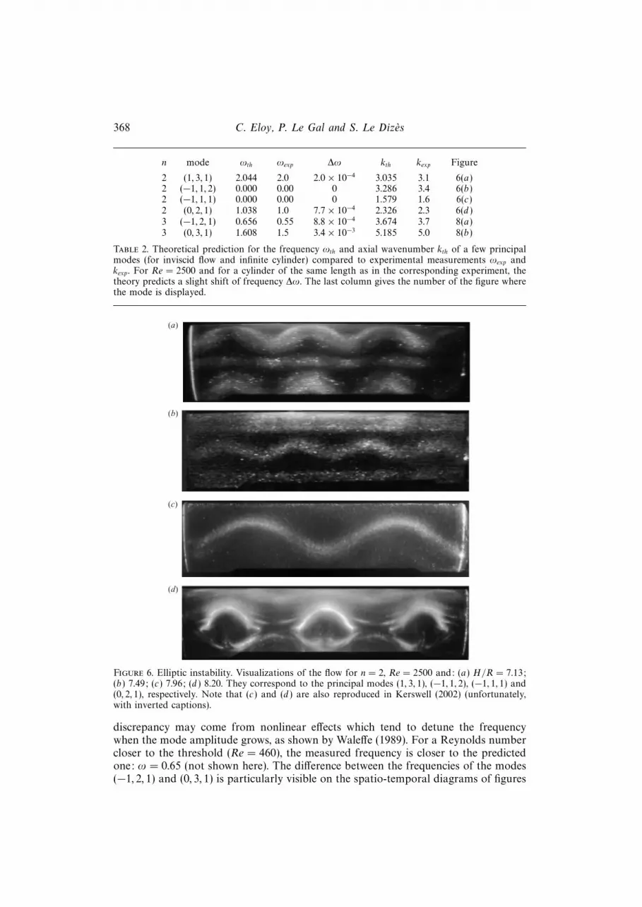
To test the mode selection by varying the aspect ratio, four experiments have beencarried out for an elliptic deformation at the same Reynolds numbers, for four differentaspect ratios (H/R = 7.13, 7.49, 7.96 and 8.20). Figure 6 shows the flow obtainedby Kalliroscope visualizations when the mode amplitude has reached saturation. Ineach case, the aspect ratio has been chosen such that an experimental wavenumberwhich is given by k = lπR/H , where l is an integer, is close to the most unstabletheoretical wavenumber of a given mode. Here, for the four different aspect ratios,we should observe the modes (1, 3, 1), (−1, 1, 2), (−1, 1, 1) and (0, 2, 1), respectively(as seen in figure 9). The most unstable wavenumbers, which are calculated for aninfinite Reynolds number and an infinite cylinder are reported in table 2 togetherwith their frequency. The experimental wavenumber can be measured by countingthe number of wavelengths observed along the cylinder (in figure 6 for instance, 3.5,4, 2 and 3 wavelengths can be identified for each aspect ratio, respectively). Thesemeasured wavenumbers kexp are not exactly equal to the theoretical most unstablewavenumbers. These slight differences in wavenumber as well as the finiteness of theReynolds number can be taken into account in the theory. They induce a small shiftin the frequencies ∆ω which is indicated in table 2. The experimental frequency isobtained by image analysis of Kalliroscope visualizations. A spatio-temporal diagramis constructed by extracting the same horizontal line in each image of the videosequence and by laying the lines on the same figure (figure 7 for instance). Thesespatio-temporal diagrams show the time-periodicity of the flow and permit us tomeasure the frequencies ωexp which are reported in table 2. Note that the modesdisplayed in figures 6(b) and 6(c) are stationary, as predicted by the theory. The twoperiodic modes shown in figures 6(a) and 6(d ) also have frequencies very close to thetheoretical predictions. These good agreements permit us to identify unambiguouslythe modes observed with the modes predicted by the theory.

The same experiments have been performed for the triangular deformation. Figure 8shows visualizations of the modes (−1, 2, 1) and (0, 3, 1) and their associated spatio-temporal diagrams. Wavelength and frequency of these modes (measured with thesame techniques as for elliptic deformation) are given in table 2. However, thefrequency of the mode (−1, 2, 1) at Re = 1200, measured in figure 8(c), is ω = 0.55.This value is different from the theoretical prediction which is ω = 0.656. This

368 C. Eloy, P. Le Gal and S. Le Dizes

n mode ωth ωexp ∆ω kth kexp Figure

2 (1, 3, 1) 2.044 2.0 2.0× 10−4 3.035 3.1 6(a)2 (−1, 1, 2) 0.000 0.00 0 3.286 3.4 6(b)2 (−1, 1, 1) 0.000 0.00 0 1.579 1.6 6(c)2 (0, 2, 1) 1.038 1.0 7.7× 10−4 2.326 2.3 6(d )3 (−1, 2, 1) 0.656 0.55 8.8× 10−4 3.674 3.7 8(a)3 (0, 3, 1) 1.608 1.5 3.4× 10−3 5.185 5.0 8(b)

Table 2. Theoretical prediction for the frequency ωth and axial wavenumber kth of a few principalmodes (for inviscid flow and infinite cylinder) compared to experimental measurements ωexp andkexp. For Re = 2500 and for a cylinder of the same length as in the corresponding experiment, thetheory predicts a slight shift of frequency ∆ω. The last column gives the number of the figure wherethe mode is displayed.

(a)

(b)

(c)

(d)

Figure 6. Elliptic instability. Visualizations of the flow for n = 2, Re = 2500 and: (a) H/R = 7.13;(b) 7.49; (c) 7.96; (d ) 8.20. They correspond to the principal modes (1, 3, 1), (−1, 1, 2), (−1, 1, 1) and(0, 2, 1), respectively. Note that (c) and (d ) are also reproduced in Kerswell (2002) (unfortunately,with inverted captions).

discrepancy may come from nonlinear effects which tend to detune the frequencywhen the mode amplitude grows, as shown by Waleffe (1989). For a Reynolds numbercloser to the threshold (Re = 460), the measured frequency is closer to the predictedone: ω = 0.65 (not shown here). The difference between the frequencies of the modes(−1, 2, 1) and (0, 3, 1) is particularly visible on the spatio-temporal diagrams of figures

Elliptic and triangular instabilities in rotating cylinders 369

1 2 76543

35

30

25

20

15

10

5

Ωt

z /R

Figure 7. The spatio-temporal diagram of the mode (1, 3, 1). Experimental parameters are n = 2,Re = 2500 and H/R = 7.13. The signal is here time-periodic with a frequency ωexp = 2Ω where Ωis the angular frequency of the cylinder rotation.

0 321z /R

1055

1060

1065

(b)

(d )

(a)

(c)

0 321z /R

670

675

680

685

Ω t

Figure 8. Triangular instability. Visualizations of the modes (a) (−1, 2, 1) and (b) (0, 3, 1). Exper-imental parameters are: n = 3, Re = 1200 and (a) H/R = 3.4, (b) 3.8. The spatio-temporal diagrams(c) and (d ) correspond to visualizations (a) and (b), respectively.

8(c) and 8(d ) where the time axes have the same scale. Several radial structures havebeen observed in the Kalliroscope visualization. However, as already mentioned, itis hazardous to associate them with any radial structure of the velocity field (seeGauthier et al. 1998).

370 C. Eloy, P. Le Gal and S. Le Dizes

7.2 7.47.0 7.8 8.07.6 8.2 8.4

105

104

103

102

Re

104

103

102

Re

(1,3,1) (–1,1,2) (–1,1,1) (0,2,1)

(a)

(b)

(0,3,1)

(1,4,1)

(2,5,1)

(–1,2,1)

3 4 5 6 7 8H /R

Figure 9. Comparison of the predicted and observed principal mode as a function of the exper-imental control parameters (H/R, Re) for (a) n = 2 and (b) n = 3. Each grey tone corresponds to themost dangerous principal mode, i.e. the mode with the largest growth rate. The symbols representexperiments: (a) ©, (−1, 1, 1); ∗, (−1, 1, 2); 4, (0, 2, 1); +, (1, 3, 1) and (b) ©, (−1, 2, 1); +, (0, 3, 1).×, visualizations where no distinct mode was observed.

The comparison between theoretical predictions and experimental observationsis summarized in figure 9. For each experiment (a single symbol in figure 9), theobserved principal mode is reported and compared to the most unstable modefound theoretically. In the elliptic case, the agreement is excellent except close to thethreshold where no distinct principal mode has been observed. This is probably dueto the small amplitude of the mode for low Reynolds numbers in agreement with thesupercriticality of the bifurcation (Mason & Kerswell 1999). It will be seen in § 4.2,that PIV permits us to observe the mode (−1, 1, 1) closer to the threshold.

In the triangular case (figure 9b), there is good agreement between the observedand predicted principal modes close to the threshold. However, when the Reynoldsnumber is increased, the mode predicted by linear stability theory is not recoveredexperimentally. Indeed, we always observe the same mode as the Reynolds number isincreased. This phenomenon could be related to either nonlinear or transient effects.

Elliptic and triangular instabilities in rotating cylinders 371

Unusual effects have also been found for H/R = 3.8, Re = 4300 and 5500. For theseparameters, a non-periodic cycle between the principal modes (−1, 2, 1) and (0, 3, 1)has been observed reproducibly.

4.2. The stationary undulating mode (−1, 1, 1)

In this section, we focus on the stationary mode (−1, 1, 1) which was previouslyobserved in a similar experiment by Malkus (1989) and by Malkus & Waleffe (1991).This particular mode can be observed for an elliptic deformation of the cylinder(n = 2), for an aspect ratio ranging from H/R = 7.7 to 8 and for a large rangeof Reynolds numbers (as described by figure 9). All the results presented in thefollowing were obtained for an aspect ratio of H/R = 7.96 which corresponds tothe visualization of two wavelengths of the mode (−1, 1, 1) along the length ofthe cylinder. We first present the characteristics of the flow produced by the mode(−1, 1, 1), then the theoretical results obtained by a weakly nonlinear analysis. Finally,the experimental results obtained by PIV measurements are compared to the theory.

By definition, the principal mode (−1, 1, 1) is the sum of two counter helicalstationary modes which give rise to a stationary wave. If we neglect the ellipticdeformation of the streamlines, the total velocity field can be written, in the linearregime, as

v(r, θ, z) =

0r0

+ 2a

Ur(r) cos(kz) sin(θ − ϕ)Uθ(r) cos(kz) cos(θ − ϕ)Uz(r) sin(kz) sin(θ − ϕ)

, (4.1)

where the first term corresponds to the solid-body rotation and the second term isthe stationary wave of complex amplitude A = ae−iϕ, where a and ϕ are two realnumbers. The functions Ur(r), Uθ(r) and Uz(r) are given in the Appendix. To satisfythe inviscid boundary conditions, the radial velocity is such that Ur(1) = 0 and theaxial wavelength k such that kH/R = 4π, i.e. k = 1.579 as shown in the previoussection. There are particular points within the cylinder where the velocity field isexactly zero. The coordinates (r, θ, z) of these points are such that sin(θ−ϕ) = 0 andr satisfies the following implicit equation

2aUθ(r) cos(kz) cos(θ − ϕ) + r = 0, (4.2)

where z can take any value. The projection of the velocity field in a plane perpendicularto the z-axis is always a rotation around a particular point whose position in theplane θ = ϕ is given by (4.2).

The position of this new rotation axis is obtained by solving (4.2) for all z. Inthe linear stability theory, the angle ϕ is predicted to remain zero: this correspondsto an undulation of the vortex centre in the plane of stretching (θ = 0). Figure 10compares a Kalliroscope visualization of the mode (−1, 1, 1) and the loci of thecentre of rotation for an amplitude a = 0.03. Note that we have taken into account,in figure 10(b), the optical effect of the convex cylinder surface which makes themode appear about 1

3larger. In figure 10(a), we can see that the demarcation line

between the dark zone and the illuminated zone corresponds remarkably well withthe position of the rotation centre in figure 10(b). For this particular mode, theKalliroscope technique would allow us to obtain quantitative information on the flowfield, which is not generally the case. Theoretically, if the rotation centre stays inthe plane of visualization, we should be able to measure the mode amplitude a as afunction of time by this method. However, this is not possible in practice as nonlineareffects tend to rotate the plane of undulation and therefore to shift the rotation centre

372 C. Eloy, P. Le Gal and S. Le Dizes

0 1 2 3 4 5 6 7 8

0

0.5

1.0

–1.0

–0.5

z /R

xapp

R

(b)

(a)

Figure 10. Comparison between visualization and theoretical prediction of the mode (−1, 1, 1).(a) Kalliroscope visualization for Re = 2500 and H/R = 7.96 in the (x, z)-plane (i.e. θ = 0) and(b) theoretical prediction of the centre of rotation by the linear stability theory for a mode amplitudeA = 0.03.

outside the plane of visualization. For this reason, we analyse experimentally the flowin a plane perpendicular to the cylinder axis and use PIV measurements to track theevolution of the rotation centre.

From a theoretical point of view, to understand the dynamics of the mode amplitudeand particularly the rotation of its phase ϕ, we have to consider the nonlinearmodification of the basic flow. Waleffe (1989) first performed a weakly nonlinearanalysis of the elliptic instability in the absence of viscosity (see also Sipp 2000)and Racz & Scott (2001b) carried out a viscous weakly nonlinear analysis of aparametric instability similar to the elliptic instability. Racz & Scott (2001b) showedthat the effects of viscosity are not as simple as initially guessed by Waleffe (1989).Finally, Mason & Kerswell (1999) performed a weakly nonlinear analysis of the ellipticinstability (in a cylinder with modified boundary conditions) focusing on the saturatedstate of the mode amplitude. Here, in order to compare theory with the PIV measure-ments, we have to perform a weakly nonlinear analysis of the elliptic instabilityincluding viscous effects and dynamical effects. Since the analysis is quite long anddoes not involve new methods, the reader is referred to the above papers for technicaldetails. In the present paper, we merely outline the analysis for the distinguishedscaling and we then jump to the amplitude equations.

Following classical asymptotic methods, the amplitude A is expanded in powersof the small eccentricity ε. The distinguished scaling for weakly nonlinear effects isobtained when the amplitude is O(ε1/2). The Reynolds number is chosen to be O(ε−2)such that the viscous flow induced by boundary layers is O(ε3/2) (this viscous flow isproportional to Re−1/2A). The nonlinear correction of the basic flow forced by theprincipal mode is a O(ε) geostrophic flow. This flow has vanishing axial and radialvelocity and its azimuthal velocity v0 depends only on radius r. It can be decomposedon the basis of Bessel functions J1(K

(i)r) all vanishing in r = 1:

v0(r) =

∞∑i=1

a(i)0 J1(K

(i)r), (4.3)

with each real amplitude a(i)0 of order ε.

Elliptic and triangular instabilities in rotating cylinders 373

The amplitude A of the mode (−1, 1, 1) and the amplitudes a(i)0 are supposed to vary

on a slow time scale εt such that dA/dt = O(ε3/2) and da(i)0 /dt = O(ε2). The amplitude

equations for A and a(i)0 are therefore obtained by solvability conditions at orders

ε3/2 and ε2, respectively. At order ε3/2, the dynamics of A is driven by the interactionof the mode (−1, 1, 1) with the geostrophic mode giving rise to a flow proportionalto a

(i)0 A and by the triple interaction of the mode (−1, 1, 1) with itself producing a

flow proportional to |A|2A. The equations describing the dynamics of the geostrophicflow are obtained at order ε2. They result from the nonlinear interaction of the mode(−1, 1, 1) with the elliptic deformation and the boundary-layer corrections. Finally,both the mode (−1, 1, 1) and the geostrophic flow are damped by viscosity. Thebalance of this O(Re−1/2) damping term with the O(ε) instability growth rate justifiesa posteriori the scaling chosen for Re.

The resulting amplitude equations are (still with A = ae−iϕ):

da

dt= (εσi cos 2ϕ− Re−1/2µ0)a, (4.4a)

dϕ

dt= δ + Da2 − εσi sin 2ϕ+

∞∑i=1

ξ(i)a(i)0 , (4.4b)

da(i)0

dt= 2ελ(i)

1 a2 cos 2ϕ+ Re−1/2λ

(i)2 a

2 − Re−1/2µ(i)1 a

(i)0 , (4.4c)

with the inviscid growth rate σi = 0.5312 and the nonlinear coefficient D = 2.015.

The damping coefficients are µ0 = 0.801 + 9.97Re−1/2, µ(i)1 = 0.125 +K (i)2Re−1/2 where

the first term of µ0 and µ(i)1 originates from viscous boundary layers and the second

term from volumic viscous effects. The constants K (i) appearing in µ(i)1 and the other

coefficients λ(i)1 , λ(i)

2 and ξ(i) are given in table 3 (for i 6 4). Here, as above, we haveincluded the viscous volumic effects in the viscous coefficients µ0 and µ1 even if theyappear at a larger order. The first amplitude equation (4.4a) reflects the modificationof the growth rate when the angle ϕ is not zero. It appears that the growth ratein the weakly nonlinear regime is simply equal to the linear growth rate multipliedby the factor cos 2ϕ, which is the local normalized stretching rate for θ = ϕ. Inthis equation, the viscous damping rate Re−1/2µ0 also appears. The critical Reynoldsnumber is obtained when growth and damping rates compensate, i.e. µ0Re

−1/2 = εσi

which gives Rec = 537 (we recover the same critical Reynolds number as in the lineartheory for H/R = 8). In (4.4b), the term δ reflects the detuning associated with aspectratio variation which tends to modify the angle ϕ. In the following, the coefficientδ is assumed to be negligible, i.e. the cylinder is assumed to be perfectly tuned. In(4.4b), we can also see that the geostrophic flow modifies the angle ϕ. The thirdequation (4.4c) describes the dynamics of the geostrophic flow through the differentamplitudes a(i)

0 . It is worth noticing that the coefficients λ(i)1 , λ(i)

2 and ξ(i) rapidly decayas i increases. This permits us to justify a truncation of the sum appearing in (4.4b).It is also important to note that λ(i)

1 and λ(i)2 are of opposite sign. This means that

elliptic and viscous effects tend to compensate when considering the evolution of thegeostrophic flow.

As demonstrated by Racz & Scott (2001b) on a similar system, the equationsystem (4.4a)–(4.4c) admits non-trivial fixed points. The first equation gives theangle of those fixed points which simply satisfies cos 2ϕ = Re−1/2µ0/εσi. For thisangle, elliptic destabilizing effects are exactly balanced by viscous damping. Note

374 C. Eloy, P. Le Gal and S. Le Dizes

i K (i) ξ(i) λ(i)1 λ

(i)2

1 3.83 −0.223 −18.47 43.502 7.01 −0.153 −3.33 9.363 10.2 0.056 0.76 −2.644 13.3 −0.033 −0.33 1.45

Table 3. The different coefficients appearing in the nonlinear amplitude equations (4.4a)–(4.4c) fori 6 4. These coefficients are only valid for the mode (−1, 1, 1) and for H/R = 8.

that the amplitude a of the fixed point does not intervene in the fixed point an-gle. Figures 11 and 12 illustrate the possible dynamical behaviours of amplitudeA for different Reynolds numbers. To obtain these figures, the equation system(4.4a)–(4.4c) has been solved numerically with the initial conditions a = 10−5, ϕ = 0and a

(i)0 = 0 for all i. When the amplitude is small, the dynamics follow the property

of linear stability analysis, i.e. the amplitude a grows exponentially and ϕ remainszero. As a continues to grow, the first effect of nonlinearity is to shift the angle ϕ,thus decreasing the growth rate, as described by (4.4a). Eventually, the amplitudeA converges towards a fixed point by spiralling in the complex plane (as seen infigure 12). The oscillating behaviour is more and more pronounced as the Reynoldsnumber increases. For infinite Reynolds number, the nonlinearity has a peculiar effect.Indeed, in this case, a should eventually decrease back to zero after a given time, asstressed by Sipp (2000). However, this kind of trajectory is singular; for any finiteReynolds number, the trajectory always converges to a fixed point different fromzero.

To compare the theoretical predictions of the weakly nonlinear stability theory withexperimental results, we have performed PIV measurements. For this purpose, thecylinder is illuminated by a laser sheet in the plane z/H = 0.75, corresponding to amaximum displacement of the rotation centre. The time interval between two imagescan be varied from 5 to 100 ms according to the rotation frequency of the cylinder.As illustrated by figure 13, the PIV algorithm allows us to measure the projectionof the velocity field in the plane of the laser sheet. Thus, it provides the positionof the rotation centre. Both ϕ and a can be determined from this position. Theangle ϕ corresponds to the physical angle between the direction of stretching andthe position of this rotation centre. The amplitude a can be inferred from equation(4.2) for cos(kz) = 1, by measuring the distance r between the rotation centre and thecentre of the cylinder.

A succession of PIV analyses permits us to follow the evolution of a and ϕas a function of time. Such evolutions are shown in figure 14 for three differentReynolds numbers. For all Reynolds numbers, the first stage of the experiment isthe spin-up of the flow (not shown in these figures). During spin-up, a large part ofthe core of the cylinder is motionless, thus not permitting us to define precisely theposition of the rotation centre. After spin-up, the rotation centre is located near thecylinder centre, i.e. the mode amplitude a is small. At this stage, the measurement ofthe angle ϕ is impossible (on the left of the dashed line in figure 14b). Eventually, themode amplitude grows until it reaches a saturated state (a = 0.04 for Re = 790 anda = 0.06 for Re = 1600) and as it grows, the angle ϕ increases from zero to a fixedvalue (ϕ = 14 for Re = 790 and ϕ = 26 for Re = 1600). For Re = 1600, saturationof amplitude occurs when 300 < Ωt < 450. For larger times, another dynamic begins

Elliptic and triangular instabilities in rotating cylinders 375

0 200 400 600 800 1000

0.05

0.10(a)

(b)

Am

plit

ude

0 200 400 600 800 1000

0

Ang

le

10

20

30

40

50

60

–10

Ωt

Figure 11. Illustration of the weakly nonlinear dynamics of the amplitude A by (a) its norm a and(b) phase φ for three different Reynolds numbers: ——–, Re = 790; – – – –, 1600; · · · · · ·, 4700.

at time Ωt = 450 which converges to a slightly different fixed point (a = 0.07 andϕ = 24). This new dynamic is reproducible and appears for 1000 < Re < 4000. Forthe highest Reynolds number, Re = 4700, no saturation of the amplitude could beobserved. This case is discussed in more detail in the next section.

For Re = 790, the agreement between theory and experiment is excellent (seefigures 11 and 14), even if the amplitude a and angle ϕ of the fixed point observedin the experiment are slightly below the theoretical predictions. For Re = 1600,agreement is also quite good until Ωt = 450. After this time, a new phenomenon, nottaken into account in the weakly nonlinear theory (probably linked to a secondaryinstability as will be discussed below), comes into play and modifies the dynamics.Finally, for Re = 4700, the agreement is only correct during the exponential growthof the amplitude. After that, at time Ωt ≈ 300, the weakly nonlinear theory is notsufficient to describe the collapse of the amplitude.

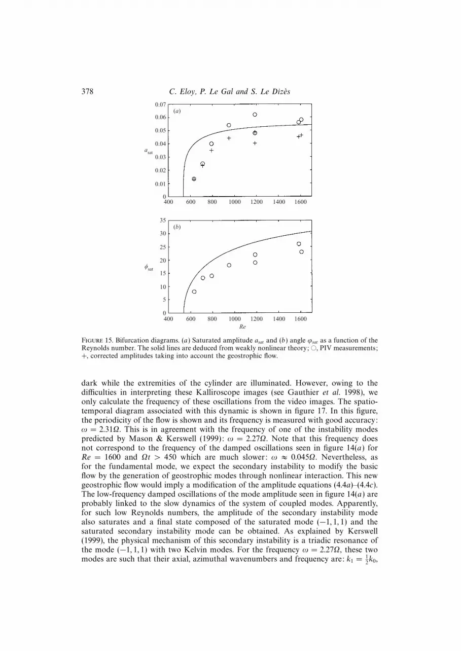
Another way of comparing between weakly nonlinear theory and experiments isto plot the measured saturated amplitude asat and saturated angle ϕsat of the fixedpoints as a function of the Reynolds number, as in figure 15. In this figure, thevalue of the first fixed point reached by the amplitude is plotted (for Re = 1600, itcorresponds to time 300 < Ωt < 450 as explained above) since we believe that thefollowing dynamics are due to higher-order nonlinear effects not taken into accountin the theory. In figure 14(a), the mode amplitude plotted is deduced from (4.2) for

376 C. Eloy, P. Le Gal and S. Le Dizes

0 0.02 0.04 0.06 0.08

0.01

0.02

0.03

0.04

0.05

0.06

Re(A)

Im(A

)

Figure 12. Trajectories of the amplitude A in the complex plane for the sameReynolds numbers as figure 11.

Figure 13. Illustration of a typical PIV velocity field of the mode (−1, 1, 1). The dashed and dottedlines represent the stretching and compression axis, respectively. Close to the cylinder wall, thevelocity field could not be measured because of illumination problems due to the presence of therollers.

cos(kz) cos(θ − ϕ) = −1. However, when a is large, an important geostrophic flowis produced which makes the amplitudes a(i)

0 in the amplitude equation system (4.4)non-negligible. Knowing the angle ϕ and given the Reynolds number, the amplitudesa

(i)0 of the geostrophic modes can be calculated at saturation using (4.4c). They are

shown to be proportional to a2. Thus, (4.2) can be modified into a second-order linearequation for a to take into account the geostrophic flow v0(r). The solutions of thiscorrected equation correspond to the crosses in figure 15(a). This corrected saturatedamplitude is about 20% lower than the amplitude shown in figure 14(a). It shows aposteriori that figure 14(a) gives only qualitative information on the mode dynamics.

From figure 15, we can see that there is a fairly good agreement between thepredicted critical Reynolds number (Rec = 537) and the one that could be inferred

Elliptic and triangular instabilities in rotating cylinders 377

0 200 400 600 800 1000

0.05

0.10(a)

(b)

Am

plit

ude

0 200 400 600 800 1000

0

Ang

le

10

20

30

40

50

60

–10

Ωt

Figure 14. PIV measurements of (a) the amplitude and (b) the angle of the mode (−1, 1, 1) as afunction of time for ∗, Re = 790; 4, 1600; ©, 4700.

from experiments. It is, however, important to mention that close to the threshold, theexperiments were difficult to carry out owing to the fatigue of the cylinder materialduring the long period of time needed by the experiment (over 3 h). In figure 15(b), themeasured saturated angle is compared with that predicted by (4.4a) for saturation. Thegood agreement confirms that the angle of saturation is simply the angle for whichthe stabilizing effect of viscosity and the destabilizing effect of ellipticity compensate.A small shift of 5 can be observed (it could be due to a lack of accuracy whendefining the direction of stretching).

For Re > 1000, a periodic dynamic is observed superimposed on the stationarymode (−1, 1, 1). This phenomenon can be associated with a secondary instabilitywhich has been identified in numerical simulations by Kerswell (1999) and Mason &Kerswell (1999) (see also Fabijonas, Holm & Lifschitz 1997; Lifschitz & Fabijonas1996). By Kalliroscope visualization, we also observed the saturated state of thissecondary instability as displayed in figure 16. As can be seen on these six successiveimages representing one period, a global oscillation of the flow is superimposed onthe basic deformation of the axis of rotation due to the primary mode (−1, 1, 1).During half a period of this secondary instability, the centre part of the flow isstrongly illuminated in contrast to the end parts which stay darker. In the followinghalf-period, the opposite situation occurs where the centre part of the flow stays

378 C. Eloy, P. Le Gal and S. Le Dizes

0

0.01

400 600

0.02

0.03

0.04

0.05

0.06

0.07

0

5

800 1000 1200 1400 1600

(a)

(b)

10

15

20

25

30

35

asat

φsat

400 600 800 1000 1200 1400 1600Re

Figure 15. Bifurcation diagrams. (a) Saturated amplitude asat and (b) angle ϕsat as a function of theReynolds number. The solid lines are deduced from weakly nonlinear theory; ©, PIV measurements;+, corrected amplitudes taking into account the geostrophic flow.

dark while the extremities of the cylinder are illuminated. However, owing to thedifficulties in interpreting these Kalliroscope images (see Gauthier et al. 1998), weonly calculate the frequency of these oscillations from the video images. The spatio-temporal diagram associated with this dynamic is shown in figure 17. In this figure,the periodicity of the flow is shown and its frequency is measured with good accuracy:ω = 2.31Ω. This is in agreement with the frequency of one of the instability modespredicted by Mason & Kerswell (1999): ω = 2.27Ω. Note that this frequency doesnot correspond to the frequency of the damped oscillations seen in figure 14(a) forRe = 1600 and Ωt > 450 which are much slower: ω ≈ 0.045Ω. Nevertheless, asfor the fundamental mode, we expect the secondary instability to modify the basicflow by the generation of geostrophic modes through nonlinear interaction. This newgeostrophic flow would imply a modification of the amplitude equations (4.4a)–(4.4c).The low-frequency damped oscillations of the mode amplitude seen in figure 14(a) areprobably linked to the slow dynamics of the system of coupled modes. Apparently,for such low Reynolds numbers, the amplitude of the secondary instability modealso saturates and a final state composed of the saturated mode (−1, 1, 1) and thesaturated secondary instability mode can be obtained. As explained by Kerswell(1999), the physical mechanism of this secondary instability is a triadic resonance ofthe mode (−1, 1, 1) with two Kelvin modes. For the frequency ω = 2.27Ω, these twomodes are such that their axial, azimuthal wavenumbers and frequency are: k1 = 1

2k0,

Elliptic and triangular instabilities in rotating cylinders 379

(a)

(b)

(c)

(d )

(e)

( f )

Figure 16. Secondary instability mode. Six successive pictures of the flow for the following exper-imental parameters: n = 2, Re = 2100 and H/R = 7.80. The first picture is taken after 3 min, i.e.Ωt = 514. The time interval between two pictures is Ω∆t = 0.54 such that the six pictures representa full period of the dynamics.

m1 = 2, ω1 = 2.27Ω and k2 = 32k0, m2 = 3, ω2 = 2.27Ω, with k0 = 1.579 the axial

wavenumber of the mode (−1, 1, 1). Mason & Kerswell (1999) predict the presenceof a secondary instability mode of frequency ω = 2.27Ω as soon as a > 0.014 (thisnumber is different from that found in their paper because of different normalizationsof the Kelvin modes). In our measurements, the oscillation of the amplitude A aftersaturation was only observed for Re > 1000 which corresponds to asat > 0.05. Thisapparent discrepancy may be due to the fact that the amplitude of the secondaryinstability has to be sufficiently large to be observed experimentally. For Re < 4000,

380 C. Eloy, P. Le Gal and S. Le Dizes

1 2 3 4 5 76

z /R

10

20

30

40

50

Ωt

Figure 17. Spatio-temporal diagram of the secondary instability mode. This diagram is constructedby extracting a horizontal video line in the top quarter of the cylinder (as seen in figure 16). Theexperimental parameters are identical to those indicated in figure 16. The signal is time-periodicwith a frequency ωexp = 2.31Ω.

we always observed the saturation of the primary mode and its secondary instability(when present). However, for higher Reynolds numbers, the flow exhibits a newbehaviour, as described in the next section.

4.3. High-Reynolds-number flow

For Re > 4000, the weakly nonlinear theory, as exposed in the previous section, isnot sufficient to describe what can be seen by Kalliroscope visualizations. For time-periodic modes of the elliptic instability (all modes different from (−1, 1, 1)), or formodes of the triangular instability (all time-periodic), no saturation of the modeamplitude has been observed. Figure 18 shows three successive pictures of the flowfor the mode (−1, 2, 1) of the triangular instability. For Re = 4700, 4.5 wavelengthsof the mode (−1, 2, 1) are first observed along the length of the cylinder (figure 18a).This oscillation grows (figure 18b) until it eventually leads after a few periods ofrotation to an apparent disordered flow (figure 18c) which is maintained forever.Unfortunately, because of the short time scale of the phenomenon affecting theseperiodic modes, it is difficult to carry out PIV measurements and the visualizationgives only a qualitative picture of the flow. The apparent small-scale disorder couldbe the result of the superposition of several modes of the multipolar instabilityand secondary instability modes. In the literature, this apparent disorder has beencalled ‘resonant collapse’ (McEwan 1971), ‘wave collapse’ (Malkus 1989), ‘breakdown’(Kerswell 1999) or ‘explosion’ (Eloy et al. 2000). In the following, we shall use theseterms indifferently even if we believe that this state could be explained by a weaklynonlinear interaction of modes as is argued below.

For the stationary mode (−1, 1, 1) of the elliptic instability, the evolution of the flowappears to be different. As mentioned in Eloy et al. (2000), there is no saturation of themode amplitude for such high-Reynolds-number flows. A cycle of instability, explosionand relaminarization can be observed with Kalliroscope visualization (figure 5 of

Elliptic and triangular instabilities in rotating cylinders 381

(a)

(b)

(c)

Figure 18. Three successive pictures of the flow [mode (−1, 2, 1)] for n = 3, Re = 4700 H/R = 8and (a) Ωt = 330; (b) Ωt = 350; (c) Ωt = 420.

Eloy et al. 2000). The first two stages are comparable to what has been observedfor time-periodic modes; the instability grows until the flow becomes very disordered(apparently), similar to what can be seen in figure 18 for the mode (−1, 2, 1). Thisdisorder which is characterized by the apparition of small scales appears suddenly(on a time scale comparable to the rotation period) and gives the impression of an‘explosion’ of the flow. However, in contrast to time-periodic modes, these ‘smallscales’ are not maintained and the flow eventually relaminarizes to a solid-bodyrotation. At this stage, the instability can grow again, leading to a characteristicintermittent cycle.

Figure 14 shows how the mode amplitude and phase vary as measured with PIVfor Re = 4700. It can be seen that the amplitude first grows exponentially untilΩt = 250. At this moment, the amplitude seems to saturate (a ≈ 0.7) as does its phase(ϕ ≈ 35). But when Ωt = 300, the ‘explosion’ occurs and the amplitude decreasesuntil Ωt = 370. During this decay, the phase varies rapidly giving the impression thatthe amplitude is spiralling back to zero. Then, from Ωt = 400 to 500, the unstablemode (−1, 1, 1) grows again until the second explosion. The PIV recording ends whenthe flow has relaminarized for the second time at Ωt = 600. During the whole cycle,the velocity field as measured by PIV is a rotation around a single point (except forvery rare velocity fields at the end of the amplitude decay for which there seem to betwo rotation centres close to each other). Moreover, the impression of ‘small scales’given by the Kalliroscope visualizations is not recovered by PIV measurements. Thismeans that during the cycle, the flow is mainly composed of the mode (−1, 1, 1).

Several scenarios have been proposed in the past to explain the violent explosionobserved on visualizations. In the context of forced Kelvin modes, McEwan (1971)first proposed that this ‘resonant collapse’ (as he named it) could be triggered by thetriadic interactions of three Kelvin waves. In the context of precessing instabilities,Kobine (1995) and Manasseh (1996) observed a similar ‘collapse’. It has been argued

382 C. Eloy, P. Le Gal and S. Le Dizes

(a)

(b)

(c)

Figure 19. Three successive pictures of the flow for Re = 6600, H/R = 8 and (a) Ωt = 61;(b) Ωt = 63; (c) Ωt = 80.

that boundary-layer instabilities or a centrifugal instability could be responsible forthis collapse. Malkus & Waleffe (1991) proposed a third scenario. They claimedthat, owing to nonlinear interactions, the basic flow enters a regime (defined bydΓ 2/dr < Γ 2/r where Γ (r) is the circulation) where Kelvin modes no longer exist.They attributed the ‘collapse’ to this regime. Finally, Mason & Kerswell (1999) andKerswell (2002) argued that the secondary instability could be the first step of abifurcation cascade (in the spirit of Ruelle–Takens) leading to the violent collapse.Despite the number of scenarios, no clear experimental fact has so far been able toclarify the mechanism of ‘explosion’.

In our experiment, we have tried to test the different scenarios. We first analysed thevelocity field given by PIV measurements. It appeared that the Rayleigh criterion forcentrifugal instability and the criterion on the circulation Γ (r) proposed by Malkus& Waleffe (1991) were never satisfied throughout the whole cycle of instabilityand explosion. These two scenarios can therefore be discarded. As explained in theprevious section, for sufficiently small Reynolds number (Re < 4000), the secondaryinstability described by Kerswell (1999) has been shown experimentally. However,it was also shown that the presence of this secondary instability does not lead toexplosion in this regime. For larger Reynolds numbers, this secondary instability isprobably also present even if it is difficult to visualize experimentally because of theshort duration of the explosion. On particular visualizations such as those in figure19, just prior to explosion, two different modes of the primary elliptic instability havebeen observed. In figure 19(a), we can see the two wavelengths characterizing themode (−1, 1, 1) and, a short time later (less than half the rotation period), a modewith 3 wavelengths in figure 19(b). A spatio-temporal diagram (not shown here)permits us to measure the period of the flow: ω = 1.0Ω, and therefore confirms thatthe second mode observed is the primary mode (0, 2, 1). This means that these twomodes can coexist before explosion. Their interaction could thus play a role in thecollapse observed later. Note, however, that this superposition of the mode (−1, 1, 1)

Elliptic and triangular instabilities in rotating cylinders 383

and (0, 2, 1) is not always observed in Kalliroscope visualizations and that it was notobserved in PIV measurements.

Based on these experimental facts, we can argue that the mechanism of ‘collapse’is likely to be a nonlinear interaction of several modes of the primary or secondaryinstability. However, it is difficult to distinguish which mode interacts with the mode(−1, 1, 1) since both the secondary instability mode and the mode (0, 2, 1) involvea Kelvin mode of azimuthal wavenumber m = 2 and with a wavelength λ suchthat 3λ = H/R. As Mason & Kerswell (1999) observed numerically, the secondaryinstability could force the mode (0, 2, 1). This may explain why it can be visible onfew visualizations. Besides, any defect of the experiment (such as a non-homogeneouscylinder material) may drive a forcing at the rotation frequency Ω which is preciselythe frequency of the mode (0, 2, 1). We can imagine that the mode (0, 2, 1) createdthis way could also force the secondary instability mode. In any case, the presenceof another mode modifies the weakly nonlinear amplitude equations obtained inthe previous section. Indeed, the equation for the geostrophic modes would have totake into account the presence of these additional modes. This could be sufficient tocompletely change the dynamics of the (−1, 1, 1) mode amplitude and generate thecycle of instability–explosion observed.

5. ConclusionIn this paper, we have studied experimentally and theoretically the stability of

a vortex subjected to a dipolar or tripolar stationary strain. The experimentalapparatus is made of an elastic deformable cylinder rotated at constant angularspeed. This cylinder is constrained by two or three rollers to deform it ellipticallyor triangularly. We have studied the flow under the variation of two dimension-less control parameters: the aspect ratio of the cylinder which can be varied bychanging its length and the Reynolds number based on the angular speed. Thethird control parameter could be the strength of the applied constraint, but its vari-ation has not been studied in the present paper. We have shown theoretically bystudying the viscous linear stability of the flow that these two control parametersare able to select particular modes of the instability. A diagram showing the mostunstable mode as a function of the Reynolds number and aspect ratio has beenconstructed (figure 9). This predicted diagram shows excellent agreement with theexperimentally observed modes close to the instability threshold. In particular, wehave exhibited time-periodic modes which were not reported by previous experimentalstudies.

The instability has also been studied for Reynolds numbers far from the thresholdfor the stationary undulating modes. For the first time, we have demonstrated thata viscous weakly nonlinear analysis is able to predict the dynamics of the modeamplitude as measured by PIV up to Re = 4000. The weakly nonlinear interactionof the mode with itself drives a geostrophic mode whose effect is to modify thebasic flow. The growth of the geostrophic mode forces a detuning of the modephase which yields a stabilizing effect. In all cases, the weakly nonlinear equationslead to stable fixed points with saturated amplitude. The amplitude of the pre-dicted fixed points depends on the Reynolds number, it compares well with thePIV measurement of the saturated mode amplitude. Through Kalliroscope visual-izations, we have also shown the presence of a secondary instability as predictedby Kerswell (1999) in his numerical study. The secondary instability mode am-plitude has been shown to saturate experimentally for Re < 4000. However, for

384 C. Eloy, P. Le Gal and S. Le Dizes

higher Reynolds number, the flow exhibits a new behaviour. After the growth ofthe unstable mode, an ‘explosion’ of the flow has been observed. This ‘collapse’ isprobably due to the growth of a geostrophic mode driven by the nonlinear inter-action of secondary instability modes or other modes of the primary instability. Thisgeostrophic mode modifies the mean flow and therefore changes the dynamics ofthe mode amplitude giving the impression of a violent ‘explosion’. In other words,this apparent ‘collapse’ could be nothing but a complex weakly nonlinear interactionof the fundamental modes with secondary instability modes and the geostrophicflow.

In this paper, we have investigated the multipolar instability which is a resonantvortex instability. Its physical mechanism lies in the interaction of two natural Kelvinmodes of the vortex with the applied constraint. In the case studied here, the con-straint can be viewed as a two-dimensional stationary intrinsic ‘mode’, i.e. with axialwavenumber, azimuthal wavenumbers and frequency k = 0, m = n and ω = 0. Inthe context of turbulent flows, it would be interesting to study the effect of anygeneral intrinsic mode [k;m;ω]. Indeed, combinations of such general modes wouldgive a model of the turbulent field surrounding vortex filaments. Such a constraint islikely to drive a resonant instability similar to the multipolar instability. The richnessof this kind of resonant instability could explain the splitting and undulation ofvortex filaments seen in turbulent flows both experimentally (Cadot et al. 1995) andnumerically (Arendt et al. 1998).

We would like to acknowledge the valuable help of Patrice Meunier during theexperimental study.

Appendix. Mathematical expressionsA.1. Kelvin modes

The velocity–pressure field of a Kelvin mode is defined by (3.2) where U = (−iUr;Uθ;Uz;P ) is given by:

Ur(r) = (m− ω)δJ ′|m|(δr) +2m

rJ|m|(δr), (A 1a)

Uθ(r) = 2δJ ′|m|(δr) +m(m− ω)

rJ|m|(δr), (A 1b)

Uz(r) = − k

m− ω [4− (m− ω)2]J|m|(δr), (A 1c)

P (r) = [4− (m− ω)2]J|m|(δr), (A 1d)

where Jµ is the Bessel function of the first kind and J ′µ its derivative. The scalar δ inthese expressions is the ‘radial wavenumber’ and is defined as:

δ2 =k2(2 + m− ω)(2− m+ ω)

(m− ω)2. (A 2)

The dispersion relation D(k, m, ω) = 0 is given by

D(k, m, ω) = (m− ω)δJ ′|m|(δ) + 2mJ|m|(δ). (A 3)

Elliptic and triangular instabilities in rotating cylinders 385

A.2. Operators

The operators required to calculate amplitude equations (3.4a), and (3.4b) are:

J =

1 0 0 0

0 1 0 0

0 0 1 0

0 0 0 0

, (A 4)

Q =

0 0 0 0

0 0 0 0

0 0 0 1

0 0 1 0

, (A 5)

N =1

2

D1 − (n− 1)rn−2 −i(n− 2)rn−2 0 0

−inrn−2 D1 + (n− 1)rn−2 0 0

0 0 D1 0

0 0 0 0

, (A 6)

with

D1 = −rn−1 ∂

∂r+ mrn−2, (A 7)

L =

D2 − 1

r2−2im

r20 0

2im

r2D2 − 1

r20 0

0 0 D2 0

0 0 0 0

, (A 8)

and

D2 =1

r

∂

∂r+∂2

∂r2− m2

r2+

∂2

∂z2. (A 9)

A.3. Linear amplitude equations

As in Moore & Saffman (1975) and Eloy & Le Dizes (2001), linear amplitudeequations are obtained from solvability conditions. Explicit and compact expressionsfor the linear coefficients can be obtained if we introduce the scalar product:

〈X |Y 〉 =

∫ 1

0

(XrYr +XθYθ +XzYz +XpYp)r dr, (A 10)

and the notation:

N2|1 = 〈U (2)|NU (1)〉, (A 11)

where U (1) and U (2) are the velocity–pressure fields of the first and second Kelvinmodes, respectively. Using similar techniques to those in Eloy & Le Dizes (2001), weobtain for the coefficients appearing in (3.4a) and (3.4b)

n1 =N1|2 − I1

J1|1, v1 = −L1|1

J1|1, q1 =

Q1|1J1|1

, (A 12a–c)

386 C. Eloy, P. Le Gal and S. Le Dizes

n2 =N2|1 − I2

J2|2, v2 = −L2|2

J2|2, q2 =

Q2|2J2|2

, (A 12d–f )

where the bar denotes complex conjugation, the terms I1 and I2 originate from theinviscid elliptic boundary conditions and are evaluated in r = 1:

I1 = 12P (1)

(U

(2)θ +

1

n

∂U(2)r

∂r

), (A 13a)

I2 = 12P (2)

(U

(1)θ − 1

n

∂U(1)r

∂r

). (A 13b)

The terms s1 and s2 come from the viscous boundary conditions. Kudlick (1966) gaveexplicit expressions:

s1 =(4− ζ2

1 )

4√

2(m21 + k2 + 1

2m1ζ1)

R

H

[(1− i)

2− ζ1√2 + ζ1

(m2

1 + k2 +2m1ζ1

2− ζ1

)(A 14a)

+ (1 + i)2 + ζ1√2− ζ1

(m2

1 + k2 +2m1ζ1

2 + ζ1

)+ (1− i)

(m2

1 + k2) HR

√ζ1

], (A 14b)

s2 =(4− ζ2

2 )

4√

2(m22 + k2 − 1

2m2ζ2)

R

H

[(1 + i)

2− ζ2√2 + ζ2

(m2

2 + k2 − 2m2ζ2

2− ζ2

)(A 14c)

+ (1− i)2 + ζ2√2− ζ2

(m2

2 + k2 − 2m2ζ2

2 + ζ2

)+ (1 + i)

(m2

2 + k2) HR

√ζ2

], (A 14d)

with

ζ1 = |ω − m1|, ζ2 = |ω − m2|. (A 15a, b)

REFERENCES

Aldridge, K., Seyed-Mahmoud, B., Henderson, G. & van Wijngaarden, W. 1997 Ellipticalinstability of the Earth’s fluid core. Phys. Earth Planet. Int. 103, 365–374.

Arendt, S., Fritts, D. C. & Andreassen, Ø. 1998 Kelvin twist waves in the transition to turbulence.Eur. J. Mech. B/Fluids 17, 595–604.

Bayly, B. J. 1986 Three-dimensional instability of elliptical flow. Phys. Rev. Lett. 57, 2160–2163.

Bayly, B. J., Holm, D. D. & Lifschitz, A. 1996 Three-dimensional stability of elliptical vortexcolumns in external strain flows. Phil. Trans. R. Soc. Lond. A 354, 895–926.

Bayly, B. J., Orszag, S. A. & Herbert, T. 1988 Instability mechanisms in shear-flow transition.Annu. Rev. Fluid Mech. 20, 359–391.

Billant, P., Brancher, P. & Chomaz, J.-M. 1999 Three dimensional stability of a vortex pair. Phys.Fluids 11, 2069–2077.

Burgers, J. M. 1948 A mathematical model illustrating the theory of turbulence. Adv. Appl. Mech.1, 171–199.

Cadot, O., Douady, S. & Couder, Y. 1995 Characterization of the low pressure filaments inthree-dimensional turbulent shear flow. Phys. Fluids 7, 630–646.

Chernous’ko, Y. L. 1978 An experimental study of secondary multi-eddy flows in elliptical cylinders.Izv. Akad. Nauk SSSR FAO 14, 151–153.

Eloy, C. & Le Dizes, S. 1999 Three-dimensional instability of Burgers and Lamb–Oseen vorticesin a strain field. J. Fluid Mech. 378, 145–166.

Eloy, C. & Le Dizes, S. 2001 Stability of the Rankine vortex in a multipolar strain field. Phys.Fluids 13, 660–676.

Eloy, C., Le Gal, P. & Le Dizes, S. 2000 Experimental study of the multipolar vortex instability.Phys. Rev. Lett. 85, 3400–3403.

Elliptic and triangular instabilities in rotating cylinders 387

Fabijonas, B., Holm, D. D. & Lifschitz, A. 1997 Secondary instabilities of flows with ellipticalstreamlines. Phys. Rev. Lett. 78, 1900–1903.

Gauthier, G., Gondret, P. & Rabaud, M. 1998 Motions of anisotropic particules: application tovisualization of three-dimensional flows. Phys. Fluids 10, 2147–2154.

Gledzer, E. B., Dolzhanskiy, F. V., Obukhov, A. M. & Ponomarev, V. M. 1975 An experimentaland theoretical study of the stability of motion of a liquid in an elliptical cylinder. Izv. Acad.Sci. USSR Atmos. Oceanic Phys. 11, 617–622.

Gledzer, E. B., Novikov, Y. V., Obukhov, A. M. & Chusov, M. A. 1974 An investigation of thestability of liquid flows in a three-axis ellipsoid. Izv. Acad. Sci. USSR Atmos. Oceanic Phys. 10,69–71.

Gledzer, E. B. & Ponomarev, V. M. 1992 Instability of bounded flows with elliptical streamlines.J. Fluid Mech. 240, 1–30.

Greenspan, H. P. 1968 The Theory of Rotating Fluids. Cambridge University Press.

Jimenez, J. & Wray, A. A. 1998 On the characteristics of vortex filaments in isotropic turbulence.J. Fluid Mech. 373, 255–285.

Kelvin, Lord 1880 Vibrations of a columnar vortex. Phil. Mag. 10, 155–168.

Kerswell, R. R. 1994 Tidal excitation of hydromagnetic waves and their damping in the earth.J. Fluid Mech. 274, 219–241.

Kerswell, R. R. 1999 Secondary instabilities in rapidly rotating fluids: inertial wave breakdown.J. Fluid Mech. 382, 283–306.

Kerswell, R. R. 2002 Elliptical instability. Annu. Rev. Fluid Mech. 34, 83–113.

Kerswell, R. R. & Barenghi, C. F. 1995 On the viscous decay rates of inertial waves in a rotatingcylinder. J. Fluid Mech. 285, 203–214.

Kerswell, R. R. & Malkus, W. V. R. 1998 Tidal instability as the source for Io’s magneticsignature. Geophys. Res. Lett. 25, 603–606.

Kida, S. & Ohkitani, K. 1992 Spatiotemporal intermittency and instability of a forced turbulence.Phys. Fluids A 4, 1018–1027.

Kobine, J. J. 1995 Inertial wave dynamics in a rotating and precessing cylinder. J. Fluid Mech. 303,233–252.

Kudlick, M. 1966 On the transient motions in a contained rotating fluid. PhD thesis, MassachussetsInstitute of Technology.

Le Dizes, S. & Eloy, C. 1999 Short-wavelength instability of a vortex in a multipolar strain field.Phys. Fluids 11, 500–502.

Leweke, T. & Williamson, C. H. K. 1998a Cooperative elliptic instability of a vortex pair. J. FluidMech. 360, 85–119.

Leweke, T. & Williamson, C. H. K. 1998b Three-dimensional instabilities in wake transition. Eur.J. Mech. B/Fluids 17, 571–586.

Lifschitz, A. & Fabijonas, B. 1996 A new class of instabilities of rotating fluids. Phys. Fluids 8,2239–2241.

McEwan, A. D. 1971 Degeneration of resonantly-excited standing internal gravity waves. J. FluidMech. 50, 431–448.

Malkus, W. V. R. 1989 An experimental study of global instabilities due to tidal (elliptical) distortionof a rotating elastic cylinder. Geophys. Astrophys. Fluid Dyn. 48, 123–134.

Malkus, W. V. R. & Waleffe, F. A. 1991 Transition from order to disorder in elliptical flow: adirect path to shear flow turbulence. In Advances in turbulence III (ed. A. V. Johansson &P. H. Alfredsson). Springer.

Manasseh, R. 1996 Nonlinear behaviour of contained inertia waves. J. Fluid Mech. 315, 151–173.

Mason, D. M. & Kerswell, R. R. 1999 Nonlinear evolution of the elliptical instability: an exampleof inertial breakdown. J. Fluid Mech. 396, 73–108.

Meunier, P. & Leweke, T. 2001 Three-dimensional instability during vortex merging. Phys. Fluids13, 2747–2750.

Meunier, P. & Leweke, T. 2002 Analysis and minimization of errors due to high gradients inparticle image velocimetry. Exps. Fluids (submitted).

Moffatt, H. K., Kida, S. & Ohkitani, K. 1994 Stretched vortices – the sinews of turbulence;large-Reynolds-number asymptotics. J. Fluid Mech. 259, 241–264.

Moore, D. W. & Saffman, P. G. 1975 The instability of a straight vortex filament in a strain field.Proc. R. Soc. Lond. A 346, 413–425.

388 C. Eloy, P. Le Gal and S. Le Dizes

Passot, T., Politano, H., Sulem, P.-L., Angilella, J. R. & Meneguzzi, M. 1995 Instability ofstrained vortex layers and vortex tube formation in homogeneous turbulence. J. Fluid Mech.282, 313–338.

Pierrehumbert, R. T. 1986 Universal short-wave instability of two-dimensional eddies in an inviscidfluid. Phys. Rev. Lett. 57, 2157–2160.

Prochazka, A. & Pullin, D. I. 1998 Structure and stability of non-symmetric Burgers vortices.J. Fluid Mech. 363, 199–228.

Pullin, D. I. & Saffman, P. G. 1998 Vortex dynamics in turbulence. Annu. Rev. Fluid Mech. 30,31–51.

Racz, J.-P. & Scott, J. F. 2001a Instability in a rotating cylinder with sinusoidal compression.Part 1. Linear theory. J. Fluid Mech. (submitted).

Racz, J.-P. & Scott, J. F. 2001b Instability in a rotating cylinder with sinusoidal compression.Part 2. Weakly nonlinear theory. J. Fluid Mech. (submitted).

Rieutord, M. & Valdetarro, L. 1997 Inertial waves in a rotating spherical shell. J. Fluid Mech.341, 77–99.

Seyed-Mahmoud, B., Henderson, G. & Aldridge, K. 2000 A numerical model for ellipticalinstability of the Earth’s fluid outer core. Phys. Earth Planet. Int. 117, 51–61.

Sipp, D. 2000 Weakly nonlinear saturation of short-wave instabilities in a strained Lamb–Oseenvortex. Phys. Fluids 12, 1715–1729.

Ting, L. & Tung, C. 1965 Motion and decay of a vortex in a nonuniform stream. Phys. Fluids 8,1039–1051.

Tsai, C.-Y. & Widnall, S. E. 1976 The stability of short waves on a straight vortex filament in aweak externally imposed strain field. J. Fluid Mech. 73, 721–733.

Waleffe, F. 1989 The 3D instability of a strained vortex and its relation to turbulence. PhD thesis,Massachusetts Institute of Technology.

Watkins, W. B. & Hussey, R. G. 1977 Spin-up from rest in a cylinder. Phys. Fluids 20, 1596–1604.

Wedemeyer, E. H. 1964 The unsteady flow within a spinning cylinder. J. Fluid Mech. 20, 383–399.