experiment of free-falling cylinders in water
TRANSCRIPT
177
Technic
al P
aper
doi103723ut32177 Underwater Technology Vol 32 No 3 pp 177ndash191 2014 wwwsutorg
Experiment of free-falling cylinders in water
Sirous YasseriSafe Sight Technology Surrey UK
Received 24 February 2014 Accepted 11 August 2014
AbstractTrajectory of objects falling into water and their landing point and orientation are of interest for the protection of oil and gas production equipment resting on the seabed Falling of small-scale model cylinders through water with low velocity has been investigated experimentally Several experiments have been conducted by dropping model cylinders with the density ratio higher than 1 into a pool The main objectives were to observe the trajectory and the landing point Similar experimental results published by other researchers are reformulated to give common normalised landing points which were then used to compare with the authorrsquos tests
Keywords cylinder drop experiments offshore dropped objects submerged trajectory
1 IntroductionStudy of falling rigid bodies through water with low water entry speed (less than 10ms) has great safety significance for protection of subsea equipment from impact The trajectory of an object through water governs the impact velocity impact angle and impact point Many random parameters affect such outcomes which can only be quantified in sta-tistical terms
The non-linear behaviour of some shapes further complicates the prediction of their trajectory and the landing point Even a simple shape such as a cylinder or sphere dropped with the same nominal initial conditions lands at different points Simple solid body motions can develop chaotic behaviour given small perturbations to initial condition or changes in condition of the medium (eg density and current) along the objectrsquos path
The present paper reports the results of drop tests of cylindrical models The overall premise of the experiment consists of dropping various cylindrical
models into water recording their landing location and observing their underwater trajectory over the course of their descent The visual observation of trajectories was sketched and also noted in a descriptive way The primary purpose of the exper-iment was to determine where a dropped cylinder lands The secondary objective was the trajectory and angle of impact as this has some implication on the level of damage that a dropped object can impart
These experiments were performed in a 25m (nominal) deep pool with the assistance of a diver Nine cylindrical models were produced and dropped from a fixed height (to achieve a consistent initial velocity) and entry angle Models were retrieved after all nine of them were dropped and results recorded
A number of variables govern where an object lands if accidentally dropped The most important variables are
bullThe objectrsquos shape ndash ie if it is long cylindrical flat or boxed shaped
bullMass drag and inertial coefficientsbullThe inclination of the object at the time of dropbullThe initial velocity at the time of dropbullThe relative position of the centre of buoyancy
and the centre of gravity as this causes the object to rotate
bullEnvironmental condition namely if the sea is calm (sea surface undulation) and the current velocity
The chance combination of these factors causes an object that is dropped several times from the same point to land at different locations
Heterogeneous state of the ocean currents changing with depth and time variations of the water density and salinity are among the important factors that could change the trajectories In order to analytically replicate a specific experimental tra-jectory it is necessary to have precise knowledge of E-mail address sirousyasserigmailcom
Yasseri Experiment of free-falling cylinders in water
178
all these factors at the time of drop Since this information is often difficult to quantify reliably it appears that the flight of free-falling objects can only be described statistically
Objects that will be lifted offshore can be con-veniently categorised into four groups
1 Heavy objects such as blowout preventer (BOP) Christmas tree manifold drill-pipe bundle and coiled tubing lift frame
2 Medium-weight but bulky objects such as accu-mulator mud-mat container support for subsea distribution unit and completion basket
3 Lighter-weight but bulky objects such as lifting frame tie-in spool support
4 Light-weight long objects such as running strings and objects less than 2 tonnes
Accurate numerical modelling depends primar-ily on the ability to numerically describe complex three-dimensional dynamic behaviour and requires correct accounting of all the forces acting on the falling object Under ideal conditions the water col-umn is usually represented as a semi-infinite space with isotropic and constant properties such as tem-perature salinity and density Under these condi-tions it has been shown that an idealised cylindrical body free falling through the water could reach a number of stable or quasi-stable motion patterns (Allen 2006) Depending on the geometry and distribution of mass a range of trajectories can be expected Several distinct patterns can be observed such as straight spiral flip flat and seesaw (Chu et al 2005) In addition a single trajectory may consist of a single pattern or any combination of these trajectories
A problem with model testing is hydrodynamic scaling with respect to the water depth which has a pronounced effect on where the model lands The trajectory patterns of falling objects are affected by the mass size and shape of the models among other things
2 Industry practiceProtection of subsea assets around a platform or a drilling vessel is necessary for the safety of people working on the surface this includes environmen-tal protection as well as limiting the commercial loss There were attempts in the past to gain insight into the three questions of landing point angle of attack and trajectory A few published results have been reviewed in the present paper and their results are compared with the current experiments
A major industry code of practice is the Det Norske Veritas (DNV) recommended practice (RP) F107 (2010) which has targeted the protection of
the submarine pipelines against dropped objects DNV assumes that the landing point of an acciden-tally dropped object can be represented by a normal distribution (Fig 1)
p x expx
( )= minus
1
2
12
2
πδ δ (1)
where x is the horizontal excursion and δ is the standard deviation DNV (2010) gives the standard deviation as a function of weight and shape of the falling object and the water depth (d) The stand-ard deviation (δ) is given by
δ = dtan (α) (2)
where α is the spread in the descent angle which can be found in Table 10 of the DNV-RP-F107 (2010) code
The probability that the object lands within a horizontal distance (r) of the drop point is given by the equation
P x r p x dxr
r
(| | ) ( )le =minusint (3)
When considering object excursion in deep water the spreading of longflat objects will increase down to a depth of approximately 180m Below this depth DNV assumes spreading does not increase significantly and tends to become vertical
Parameters used in Equation 1 account for a nominal current (DNV 2010) The effect of cur-rents becomes more pronounced in deeper water because the time it takes for an object to land on the seabed will increase as the depth increases This means that any current may increase the excursion (in one direction) At 1000m depth the excursion
Fig 1 Landing point of falling objects according to DNV-RP-107
179
Underwater Technology Vol 32 No 3 2014
could be 10ndash25m for an average current velocity of about 025ms and up to 200m for a current of 10ms Only light objects with large surface areas can glide and move further away from the drop point
Regarding the installation of subsea equipment it is necessary to determine how far an object would drift if accidentally dropped This is known as the lsquostandoff pointrsquo which identifies how far an instal-lation vessel should be located from a subsea asset to avoid damage should an object be accidentally dropped overboard For this purpose rigid body dynamics of falling objects are used to estimate the distance from the drop and lifting points for vari-ous objects Fig 2 shows the standoff distances for typical offshore equipment from the point of drop for three different current velocities (no wave) using the most probable values for drag added mass and inertia coefficients
This also involves calculating the hydrodynamic loads Data were produced for a water depth of 200m The objects were released from a static posi-tion at the mean water level and their free-fall tra-jectory in the water column was tracked until they landed on the seabed Current loading applied along the vertical axis and the drift of object from the vertical axis was monitored The hydrodynamic loads were calculated by hand assuming either a plate or cylindrical shape for the objects These results are useful provided they are realistic and
not too conservative Tests that are reported in the present paper provide some further insight
Experimental results can be replicated using the dynamics of objects falling through water (see Appendix A) if the actual data are available or the input data can be manipulated to match the exper-imental results Naturally in a blind test any simi-larity between experimental and theoretical results is a matter of chance Conversely results of Fig 2 cannot be replicated by experiments
If the theoretical results are conservative and adopting them is not costly then there is no eco-nomical reason for further refinement If in the derivation of standoff distance instead of the most probable value the 95 confidence level was used then distances may not be sustainable For a large standoff distance the installation vessel may need to leave its work station to undertake an overboard lift at a safe distance lower the load close to the seabed and lsquowalkrsquo it back to the work station This would add substantially to the schedule perhaps without much benefit
Prior to the DNV-RP-F107 (2010) practicing engineers assumed discrete distribution of falling objects For this purpose the seabed was discre-tised into a number of rings (generally three) assuming a dropped cone (eg Yasseri 1997) A percentage of dropped objects were then assigned to each ring
Fig 2 Standoff distance measured from the drop point (for 200m water depth)
120
Standoff distance measured from the drop point for typical objects (200m water depth)
110
100
90
80
70
60
50
40
30
20
Sta
nd
off
dis
tan
ce m
easu
red
fro
m t
he
dro
p p
oin
t (m
)
10
0
Blowou
t pre
vent
er (1
15te
)
Drill p
ipe bu
ndle
(42t
e)
Coil tu
bing
lift fr
ame
(34t
e)
Man
ifold
stack
up
(32t
e)
Conta
iner 1
2m times
8m
times 8
m (3
0te)
Conta
iner 8
m times
8m
times 8
m (2
4te)
Drill p
ipe (2
2te)
Baske
t 20m
times 4
m times
4m
(20t
e)
Christ
mas
tree
(40t
e)
Mud
mat
s amp m
atte
rs m
odule
(38t
e)
Mon
o pil
e (2
7te)
Conta
iner 2
0m times
8m
times 8
m (2
0te)
SDU amp su
ppor
t (18
te)
Fram
e str
uctu
re (2
5te
)
Baske
t 5m
times 8
m times
8m
(20t
e)
Tie-in
spoo
l sup
port
struc
ture
(4te
)
Misc
ellan
eous
1 (5
te)
Misc
ellan
eous
2 (lt
2te)
Runnin
g str
ing (5
te)
Objects
05ms current 075ms current 1ms current
Yasseri Experiment of free-falling cylinders in water
180
3 Literature reviewFree fall of cylindrical objects has received a lot of attention in the past (eg Ingram 1991 Aanesland 1987 Colwell and Ahilan 1992 Chu et al 2004 Chu et al 2005 Chu and Fan 2006 Chu and Ray 2006 Chu 2009) In the following experimental
results available in the open literature that are rel-evant to the present paper are summarised
31 Gillesrsquo tests Gillesrsquo tests (Gilles 2001 Chu et al 2005) con-sisted of dropping circular cylinders into the water where each drop was recorded by underwater cam-eras from two viewpoints The controlled parame-ters for each drop were centre of mass (COM) position initial velocity drop angle and the ratio of cylinderrsquos length to diameter
05
Log-normal distribution fitting of Gillesrsquo tests
005
Dis
tan
ce b
etw
een
lan
din
g a
nd
dro
p p
oin
t (r
in m
)
ndash1 ndash05 05 1
Standard normal variable
15 2 25
R2 = 09521
y = 00948epx(08505r )
300
Expon (Gillesrsquo tests)Gillesrsquo tests
Fig 5 Gillesrsquo (2001) results in log-normal probably distribution plot
Fig 3 Gillesrsquo (2001) model characteristics The left-most column indicates COM position 0 while the right-most indicates COM position 2
Model No1L = 151359cm D = 4cm m = 27cm weight = 3225g
volume = 1902028cm3 density = 16956gcm3
H(cm) 10380 8052 5725
H(cm) ndash1462 0866 3193
M(mm) 0000 18468 36935
Model No2L = 120726cm D = 4cm m = 17cm weight = 2542g
volume = 151709cm3 density = 16756gcm3
H(cm) 8450 6609 4768
H(cm) ndash1546 0277 2119
M(mm) 0000 12145 24290
Model No3L = 91199 D = 4cm m = 147cm weight = 2153g
volume = 1146037cm3 density = 18786gcm3
H(cm) 6662 5592 4521
H(cm) ndash1368 ndash0297 0774
M(mm) 0000 6847 13694
Fig 4 Gillesrsquo (2001) 230 tests Plot is normalised using the water depth
Gillesrsquo 230 tests
Normalised X axis
No
rmal
ised
Y a
xis
04
03
02
01
ndash01
ndash01 01 02 03 04ndash02ndash03ndash04
ndash02
ndash03
ndash04
00
181
Underwater Technology Vol 32 No 3 2014
Fig 6 Shapes used by Ray (2006)
Rayrsquos models (2006)L
(cm)D
(cm)Mass
(g)COM(cm)
Density(gcm3)
Numberof tests
3185 483 5634 1375 2224 8
2794 402 473 142 2224 12
3175 518 831 1585 1754 11
3175 518 808 1610 1754 11
Bomb
Shell
Cylinder
Capsule
COM
COM
COM
COM
L
L
L
L
D
D
D
D
Gilles used three cylindrical shapes which had a circular diameter of 4cm however the lengths were about 15cm 12cm and 9cm respectively The bod-ies were constructed of rigid plastic with aluminium-capped ends Inside each was a threaded bolt running lengthwise across the model and an inter-nal weight The internal weight was used to vary the COM (see Fig 3) The drop angles were 15deg 30deg 45deg 60deg and 75deg This range produced velocities whose horizontal and vertical components varied in mag-nitude and allowed for comparison of trajectory sensitivity with the varying velocity components Gilles (2001) reported results for 230 tests
Gilles (2001) used five COM positions For posi-tive COM cases the COM was located below the centre of buoyancy For negative cases the COM was located above the centre of buoyancy prior to release Fig 4 shows Gillesrsquo results in normalised form The x and y coordinates were normalised by dividing them by the poolrsquos depth Circles of 10 20 30 and 40 of water depth are superim-posed on Fig 4
According to Gillesrsquo experiment 80 of objects landed within 20 of the water depth Almost 99 of objects landed within 40 of the water depth which clearly indicates a non-normal distribution contrary to the DNV assumption Fig 5 shows these results on a lognormal probability plot Appendix B shows how to determine the lognormal distribution parameters using the experimental data Direction-ality seen in Fig 4 is owing to the experimental setup All tests were done at one corner of the pool
Gilles (2001) grouped his tests into six series with the differentiating factor between the series being the drop angle However no discernible
correlation was found between the landing point and the drop angle although vertical drops were more likely to land closer to the point of drop
32 Rayrsquos testsRay (2006) used four polyester resin shapes for his experiments He reported 42 experiments using various shapes as shown in Fig 6 Dimensions of Rayrsquos model are also noted in Fig 6
The cylinder is the most predictable and stable shape of all (Ray 2006) Out of a total of 11 test runs
Fig 7 Landing point for Rayrsquos (2006) tests (42 points)
Rayrsquos tests (42 points)
Normalised X axis
No
rmal
ised
Y a
xis
05
04
03
02
01
ndash01
ndash02
ndash03
ndash04
ndash05
00 01ndash01ndash02ndash03ndash04ndash05 02 03 04 05
Capsule Shell Bomb Cylinder
Yasseri Experiment of free-falling cylinders in water
182
nine of the shapes exhibited an almost vertical trajectory pattern from the point of water entry to the landing point Models were launched orthogo-nal to the waterrsquos surface with initial velocities ranging from 28ms to 67ms The upper bound of velocity in offshore applications when an object hits the surface of the water is about 15ms
Fig 7 shows the landing points for all Rayrsquos 31 exp -eriments normalised using the water depth Owing to vertical entry all impact points for cylinders are within 105 of water depth Despite the high veloc-ity and nominal vertical entry impact points are somewhat away from the projection of entry point on the poolrsquos bottom Similar observations were made
Fig 8 Details of Allenrsquos (2006) models
Model Shape Dimensions (cm)No oftests
Model1
D 130Scale NA
Distance fromCOM to COV = 0
13
Model2
D 149H 133
Scale NADistance from
COM to COV = 0
9
Model3
D 150H 70Scale
COM to COV =+0373
along Z axis
15
Model4
L 160W(Back) 78
W(Front) 133H(Back) 63H(Front) 38
Scale 16COM to COV = 0
14
Mass ndash 16920gDensity ndash 1335gcm3
Mass ndash 28150gDensity ndash 1722gcm3
Mass ndash 11450gDensity ndash 1615gcm3
Mass ndash 8130gDensity ndash 1388gcm3
65cm
130cmCOM
55cm
133cm
149cm
745cm
62cm
75cm
38cm63cm
32cm
82cm
55cm
78cm133cm
160cm
16cm
70cm
150cm
COM
COM
COM
COM
COM
COM
183
Underwater Technology Vol 32 No 3 2014
by Bushnell (2001) where he fired missiles at 380ms into a pond from a nominal vertical direction
33 Allenrsquos testsAllen (2006) experimented with small samples in a 25m-deep pool using four shapes These shapes are shown in Fig 8 The model included a sphere that is symmetric and has equal weight distribution about its three axes
Fig 9 shows the landing point for all shapes in Allenrsquos tests Again the same pattern emerges ie dispersion clustering within 20 of the depth Some of the hemi-spherical shapes landed beyond this limit However no excursion extended beyond 50 of the depth and the largest excursion was for flat-shape objects Allenrsquos (2006) results also follow a lognormal distribution
Bushnell (2001) fired missiles into a pond at high velocity (about 300ms) at angles of attack between 1 and 35deg In addition the test specimen had tail fins some of which broke during the test In Bushnellrsquos test most missiles hit the pond floor within a circle of 02 of the water depth Bushnell experimented with missiles at a high velocity through the water where flow separation creates a cavity of air around the body That cavity is also called cavi-tation which remains in the water long after the missile has passed to influence the trajectory
4 Current model testsThe authorrsquos experiments consisted of dropping three cylindrical models of various lengths and
COM location into a 25m-deep pool at low veloc-ity similar to Gillesrsquo models (2001) (see Fig 10) The entry of each model into the water was recorded by the surface experimenter A mat with gridlines was placed on the poolrsquos bottom to facilitate the record-ing of the landing points All models were num-bered as well as marked with bright colours for ease of detection
The testing was conducted by two experiment-ers One experimenter remained at the surface and was responsible for launching the models and record-ing all test data The other experimenter was inside the pool with breathing apparatus and reported the landing point and the observed trajectory to the surface experimenter for recoding No test was dis-carded However prior to the commencement of the actual testing several trial runs were attempted in order to eliminate all likely problems This trial run also provided a procedure for performing the tests No underwater cameras were used to record the trajectory of the dropped cylinders
The controlled parameters were the cylindersrsquo physical parameters (length-to-diameter ratio COM) and initial drop conditions (initial velocity and drop angle) The models were based on the assumption that a 9m tubular is dropped in 180m of water thus producing a 201 ratio The depth of the pool was ~25m From this ratio 12cm was chosen for the length of the model Two additional models 9cm and 15cm in length were also used
Fig 10 The current model
L
δ
dCOV COM
C o G of extra mass
x
Fig 11 Schematic of experimental setup
WeightEntry point
Φ
Distance toCOM
~ 25mdepth
Fig 9 Allenrsquos (2006) tests Plot is normalised using the water depth
Allenrsquos tests (51 points)
Normalised X axis
No
rmal
ised
Y a
xis
04
03
02
01
ndash01
ndash01 01 02 03 04ndash02ndash03ndash04
ndash02
ndash03
ndash04
00
Sphere-Model 1(Fig 8)
Hemisphere-Model 2(Fig 8)
Model 3 (Fig 8) Model 4 (Fig 8)
Yasseri Experiment of free-falling cylinders in water
184
for the sensitivity analysis The outer radius of all the models was 4cm
The models were constructed of rigid plastic with a cap at both ends Fig 11 shows a schematic of the experimental setup A mass was inserted inside the model (Fig 11) to vary the COM for each model A total of nine models with three different lengths and three centres of mass for each length were pro-duced Owing to symmetry by turning the models around the COM can be below or above the centre of buoyancy
After dropping all nine models the experimenter inside the pool reported the results and recovered the models The surface experimenter then signalled his readiness for the next nine tests This cycle then was repeated until all the tests for a given drop angle were concluded
The initial orientation of the drop can be set between 0deg and 90deg with 0deg being a vertical initial orientation and 90deg being horizontal Drop angles were 15deg 30deg 45deg 60deg and 75deg This produces a situa-tion where the cylinder is heading directly down-ward throughout the event If an object dropped vertically even with no initial rotation the object will still tend to acquire a horizontal velocity component as it falls through the water This results in the object impacting the seabed at a random angle and loca-tion Several trajectory patterns (straight spiral flip flat seesaw and combination) were observed during the experiment but the four patterns as shown in Fig 12 were more frequent The COM position had the largest influence on the trajectory of cylinders
The drop point scatter plot is shown in Fig 13 When the COMs and buoyancy coincided objects
Fig 12 More frequent trajectory patterns of falling cylinders (see also Chu et al 2005)
Arc trajectory Straight trajectory
Early flip Late flip
X or Y
Wat
er d
epth
(Z
)
ndash15 ndash1 ndash05 00
ndash05
ndash1
ndash15
ndash2
ndash25
05 1 15
X or Y
Wat
er d
epth
(Z
)
ndash15 ndash1 ndash05 00
ndash05
ndash1
ndash15
ndash2
ndash25
05 1 15
X or Y
Wat
er d
epth
(Z
)
ndash15 ndash1 ndash05 00
ndash05
ndash1
ndash15
ndash2
ndash25
05 1 15
X or Y
Wat
er d
epth
(Z
)
ndash15 ndash1 ndash05 00
ndash05
ndash1
ndash15
ndash2
ndash25
05 1 15
185
Underwater Technology Vol 32 No 3 2014
fell near the drop point for more than 90 of the time while a small distance between COM and the centre of volume (COV) caused the variability When the centre of buoyancy is ahead of the COM
the model flips while descending and experi-enced the largest excursion from the drop point When the drop angle is close to 90o and the centre of buoyancy and COM coincide then the descent is mostly vertical with only a slight slant When the buoyancy centre is above the mass centre models approach the floor at acute angles between 120deg and 180deg The trajectory patterns of each model type are affected by the size and shape of the mod-els The four generalised patterns were not shared among the various shapes but rather they were quite consistent within each shape type
Fig 14 shows the distance between the landing point and drop point in a lognormal probability plot It can be seen that the lognormal distribu-tion describes the probability of the landing spot fairly well Fig 15 shows results from another set of experiments where a cylinder with a length of 10cm and diameter of 12cm and a cube of 15cm times 15cm times 15cm were dropped using the same experimental setup These 140 points also follow a lognormal distbution similar to Fig 14 Fig 16 shows a few of the observed trajectories of the falling cylinder and cube in the second set of experiments
Fig 14 Authorrsquos results on a lognormal probability plot (324 points)
Probability plot of landing points for the current tests (324 points)
Standard normal variable
Dis
tan
ce b
etw
een
lan
din
g p
oin
t an
d t
he
dro
p p
oin
t
ndash3 ndash25 ndash2 ndash15 ndash1 ndash05 0 0505
005y = 01033exp(08147r)
R2 = 09828
Experimental dataExpon (Experimental data)
1 15 2 25 3
Fig 13 A plot of the landing point of all authorrsquos 324 tests
Landing points of 324 model cylinders droppedinto 25m of water
No
rmal
ised
Y a
xis
Normalised X axis
04
03
02
01
01 02 03 040
0
ndash01
ndash02
ndash03
ndash04
ndash04 ndash03 ndash02 ndash01
Yasseri Experiment of free-falling cylinders in water
186
5 Computational approachThe motion of three-dimensional rigid bodies freely falling through water has been addressed by many researchers Appendix A outlines the formu-lation necessary to track such motion MATLAB commercial software was used to solve these equa-tions Owing to a rigid body assumption tracking of one point gives enough data to plot the position of the falling object (Fig 17) Fig 18 shows some examples of trajectories using different values of control variables
These equations replicate the experimental results fairly well The method is applied to cylin-drical bodies initially released below the free sur-face in calm water Depending on the initial body orientation body aspect ratio and mass distribu-tion it is possible to identify key characteristic pat-terns of the body motion which compare remarkably with observations in the tank-drop tests The present study has a significant implica-tion to the manoeuvring of underwater vehicles Abelev et al (2007) presented experimental results of falling heavy cylindrical shapes which are in line with the authorrsquos results
6 Concluding remarksNot all falling objects travel straight downward under the influence of gravity even in the air Sometimes the falling objects follow complicated downward trajectories as they fall It is therefore
clear that any satisfactory explanation of this com-plex phenomenon must include a description of the instantaneous fluid forces experienced by the falling object as well as the inertial and gravita-tional effects that are present
Fig 16 A few of the observed trajectories for the second set of tests
Fig 17 Tracking the orientation of a falling object with position of COM lower than COV
Trajectory of a cylindrical object with heavy nose
10
0
ndash10
ndash20
ndash30
Wat
er d
epth
(m
)
Horizontal position (m)
ndash40
ndash50
ndash60
ndash70
ndash80ndash10 0 10 20 30 40 50 60 70 80
Nose position
Fig 15 Scatter plot for two shapes a short cylinder with lengthdiameter lt 1 and a small cube (140 points)
Landing points for dropped short cylinder anda cube of 150cm times 150cm times 150cm
04
03
02
01
ndash01
ndash02
ndash03
ndash04
ndash04 ndash03 ndash02 ndash01 0 01 02 03 04
Normalised X axis
No
rmal
ised
Y a
xis
0
Cylinder Drop point Box-shape
187
Underwater Technology Vol 32 No 3 2014
The entry of a solid into water or other liquids gives rise to a sequence of complex events The evolution of the air cavity behind the falling body after the initial impact significantly influences the dynamics and trajectory of low-speed projectiles (see eg Chu and Fan 2006 Chu and Ray 2006) The effect of air cavity dynamics is more pro-nounced in large body water entry Leaves tree seeds and paper cards falling in air are spectacular examples of time-dependent fluid dynamics at intermediate Reynolds numbers at which both inertial and viscous effects are important The tra-jectory of a falling card typically appears to be very complex with the card either oscillating from side to side (fluttering) or rotating and drifting side-ways (tumbling)
It is acknowledged that there are deficiencies in representing the landing point using a statistical distribution Fitting a distribution to a set of data only tells us how the dispersion would look The data behind the DNV recommendation (2010)
could not be located which makes the compari-sons between the DNV recommendation and the current experiment difficult In addition the log-normal curve may not represent the effect of all input parameters adequately It was chosen as the first approximation with an overall goal of developing a stochastic model evaluation Other distributions may be examined and could poten-tially represent the experimentally measured data better
Real objects of any significance are generally longer than 6m but still much smaller than the water depth for deepwater locations Thus the ratio of water depth to the object length is quite high Hence replicating it in a model test requires a very small model if the pool is not very deep It is desir-able that the choice of scale is representative of the offshore industryrsquos ratio of water depth to object length but at the same time it should be large enough to cover typical offshore tubular sizes The ratio of water depth to the tubular length for a
Fig 18 A few calculated trajectories for a falling cylinder with different orientation initial velocity and hydrodynamic conditions
Yasseri Experiment of free-falling cylinders in water
188
dropped tubular model of 12m in length in a water depth of 240m is 20 Therefore for a pool depth of 25m the model length should be around 120mm
Ingram (1991) surmises there is a depth beyond which an object would fall flat implying there is a single pattern in deep water However no single pattern was observed in these tests
Pulling together all tests reported here the fol-lowing observations can be made about the land-ing location of free-falling cylinders
bullAbout 50 of the time objects land within 10 of the water depth
bullAbout 80 of the time objects land within 20 of the water depth
bullAbout 90 of the time objects land within 30 of water depth
bullAbout 95 of the time objects land within 40 of water depth
bullAbout 98 of the time objects land within 50 of water depth
These tests were performed in pools where the water surface only experiences small ripples However there is significantly more undulation in the ocean surface Such undulation will cause more deviation to the object and help it to travel further (Fig 19)
ReferencesAanesland V (1987) Numerical and experimental investi-
gation of accidentally falling drilling pipes OTC 5494 19th Offshore Technology Conference April 1987 Houston USA
Abelev AV Valent PJ and Holland KT (2007) Behaviour of a large cylinder in free fall through water IEEE Journal of Ocean Engineering 32 10ndash20
Allen CR (2006) Mine drop experiment II with operational mines shapes (MIDEX II) MS Thesis Naval Postgraduate School Monterey CA USA 306pp Available at httpfacultynpsedupcchuweb_paperthesis06Mar_Allenpdf last accessed lt14 September 2014gt
Bushnell JM (2001) Tail separation and density effects on the underwater trajectory of the JDAM MS Thesis Naval Postgraduate School Monterey CA USA 88pp Available at httpcalhounnpsedupublichandle109454406 last accessed lt14 September 2014gt
Chu PC (2009) Mine impact burial prediction from one to three dimensions ASME Journal of Applied Mechanics Review 62
Chu PC and Fan CW (2006) Prediction of falling cylinder through air-water-sediment columns ASME Journal of Applied Mechanics Review 73 300ndash314
Chu PC and Ray G (2006) Prediction of high speed rigid body manoeuvring in air-water-sediment columns In Rahman M and Brebbia CA (eds) Advances in Fluid Mechanics V Southampton UK WIT Press 123ndash132
Chu PC Fan CW Evans AD and Gilles AF (2004) Triple coordinate transforms for prediction of falling cylinder through the water column Journal of Applied Mechanics 71 292ndash298
Chu PC Gilles AF and Fan CW (2005) Experiment of falling cylinder through the water column Experimental Thermal and Fluid Science 29 555ndash568
Colwill RD and Ahilan RV (1992) Reliability analysis of the behaviour of dropped objects OTC 6918 24th Offshore Technology Conference April 1992 Houston USA
Det Norske Veritas (DNV) (2010) Risk assessment of pipeline protection Recommended practice No DNV-RP- F107 Olso Norway DNV 45pp
Evans A (2002) Hydrodynamics of mine impact burial MS Thesis Naval Postgraduate School Monterey CA 2002 Available at httpcalhounnpseduhandle10945 5310show=full last accessed lt14 September 2014gt
Friedman A Zilman G and Miloh T (2003) Dynamics of a body falling in waves In Proceedings of 18th Interna-tional Workshop of Water Waves and Floating Bodies (IWWWFB) Ann Arbour MI USA
Gilles A (2001) Mine Drop Experiment (MIDEX) MS The-sis Naval Postgraduate School Monterey CA USA 446pp Available at httpfacultynpsedupcchuweb_paperthesisgillespdf last accessed lt14 September 2014gt
Ingram JG (1991) Experimental modelling and risk assess-ment of dropped offshore tubulars MS Thesis School of Industrial and Manufacturing Science Cranfield Insti-tute of Technology Cranfield UK
Kim Y Lin KY and Yue KD (2002) Motion dynamics of three-dimensional bodies falling through water In Rainey RCT and Lee SF (eds) Proceedings of 17th International Workshop of Water Waves and Floating Bodies (IWWWFB) London WS Atkins Consultants 81ndash84 Available at httpwwwiwwwfborgAbstractsiwwwfb17iwwwfb17_21pdf last accessed lt14 September 2014gt
Ray G (2006) Bomb strike experiments for mine counter-measure MS Thesis Naval Postgraduate School Monte-rey CA USA 197pp Available at httpfacultynpsedupcchuweb_paperthesis06Mar_Raypdf last accessed lt14 September 2014gt
Von Mises R (1959) Theory of Flight 1st edition New York Dover Publications Inc 629pp
Wierzbicki T and Yue DK (1986) Impact damage of Chal-lenger crew compartment Journal of Spacecraft and Rockets 23 646ndash654
Yasseri S (1997) Risk-based decision analysis for the protec-tion of marine pipelines from dropped objects In Proceed-ings of 7th International Offshore and Polar Engineering Conference Honolulu USA 251ndash256
Fig 19 The effect of undulating sea surface on the trajectory and drifting
Drift owing to object hitting the wave atdifferent location
Wave slope
Entry angle
189
Underwater Technology Vol 32 No 3 2014
Appendix A
Rigid body dynamics of a cylinder falling through waterThere are various methods of describing the motion of a rigid body see for example Von Mises (1959) Chu et al (2005) Wierzbicki and Yue (1986) Kim et al (2002) and Friedman et al (2003) In the fol-lowing equations which are needed to track the dynamics of motion of three-dimensional rigid bod-ies falling through water (Chu et al 2005) are given
Fig 20 shows a right circular symmetric cylinder whose centres of mass (X) and volume (B) are on the cylinderrsquos longitudinal axis Parameters (L d x) denote the cylinderrsquos length diameter and the dis-tance between the two points (X B) The positive case is when the centre of mass (COM) is lower than the centre of volume (COV) ie x is positive (Evans 2002)
Three orthogonal right-handed coordinate sys-tems (Fig 21) are used describe the dynamics of a falling cylinder through the water which are E-coordinate M-coordinate and F-coordinate sys-tems The body and buoyancy forces and their moments are given in the E-coordinate system the hydrodynamic forces (drag lift and inertia forces) and their moments are given in the F-coordinate and the cylinderrsquos moments of gyration are given in the M-coordinate The E-coordinate system is fixed to the Earthrsquos surface with horizontal sides as x and y axes are parallel with the Earthrsquos surface (along the two sides of the pool) and vertical direc-tion as z axis (upward positive Fig 20)
Suppose the cylinder is falling into the water The cylinder rotates around its main axis (r1) with an angle ψ1 and an angular velocity of Ω Its position
is represented by the COM and its orientation is represented by two angles ψ2 and ψ3 (Fig 3) Here ψ2 is the angle between the r1 axis and the horizon-tal plane and ψ3 is the angle between the projec-tion of the main axis in the (x y) plane and the x axis The angle (ψ2 + π2) is usually called attitude
The relative coordinate is rigidly connected with the cylinder The origin (O) of the relative coordi-nate system coincides with the COM the r1 axis is along the central line of the cylinder the r2 axis is perpendicular to the plane constructed by r1 axis and z-axis (r1-z plane) and the r3-axis lies in the (r1-z) plane and is perpendicular to r1 axis The axes (x y z) and (r1 r2 r3) follows the right-hand rule
Let V = (V1 V2 V3 ) the three components of the velocity of COM ie the origin velocity of the coor-dinate system (r1 r2 r3) The geometric centre (GC) is located at (x 0 0) if for GC below COM x gt 0 and for GC above COM x lt 0 The relative coordinate system (r1 r2 r3) is obtained by one translation and two rotations ψ2 and ψ3 of the E-coordinate system Let the position vector (P) be represented by PE and
Fig 20 M-coordinate with the COM as the origin X (im jm) x is the distance between the COV (B) and COM (X) L and d are the cylinderrsquos length and diameter (Chu et al 2005)
2
d
L2L
B
xjm
imX
z (k )
y ( j )
kmjmψ2
imo ψ3
x (i )
obull
kf
jf
ifobull
V1
V2 Vr
Fig 21 Cylinder orientation and relative coordinate system
Yasseri Experiment of free-falling cylinders in water
190
PB in the Earth and relative coordinate systems PE and PB are connected by
PE =minus
minus
cos sin
sin cos
cos sin
si
ψ ψψ ψ
ψ ψ
3 3
3 3
2 2
0
0
0 0 1
0
0 1 0
nn cosψ ψ2 20
+
lowast
lowast
lowast
P
x
y
zB
m
m
m
(A1)
where (xm ym zm) represent the position of COM in the Earthrsquos coordinate system
The motion of a solid object falling through a fluid is governed by two principles (1) momentum balance and (2) moment of momentum balance Let Vw = (Vw1 Vw2 Vw3) be the water velocity and (ω1 ω2 ω3) be the components of the angular velocity referring to the direction of the relative coordinate system Variables are made non-dimensional by
tgL
tLg
VV
gL= = =lowast lowast
lowast
ω (A2)
where g is the gravitational acceleration and L the length of the cylinder The non-dimensional momentum equations for COM are given by (Van Mises 1959)
dVdt
V VFg
w12 3 3 2 2
1+ minus =minus
+forall
lowast
ω ωρ ρ
ρψ
ρsin (A3)
dVdt
VFg
23 1
2+ =forall
lowast
ωρ
(A4)
dVdt
VFg
w32 1 2
3minus =minus
+forall
lowast
ωρ ρ
ρψ
ρcos (A5)
where forall is the volume of the cylinder ρ is the cylinder density ρw is the water density and (F1
F2 F3
) are the components of fluid drag The non-dimensional equations of the moment of momentum for circu-lar symmetric cylinder are
ddt
J JJ
LMg J
Ω+
minus=
lowast3 2
12 3
1
1
ω ω (A6)
ddt
x LJ
LMg J
wω ρ ρψ2
22
2
2
= minusforall minus
+lowast lowast( )
cos (A7)
ddt
LMg J
ω3 3
3
=lowast
(A8)
where x is the distance between COM and GC and (M1
M2 M3
) are the components of the moment
owing to drag (J1 J2 J3) The three moments of gyration are
J r r dm J r r dm
J r r dm
1 22
32
2 32
12
3 12
22
= + = +
= +
int intint
lowast lowast
lowast
( ) ( )
( )and (A9)
The orientation of the cylinder (ψ2 ψ3) is deter-mined by
ddt
ddt
ψω ψ
ψω2
2 23
3= = cos (A10)
The eight non-dimensional nonlinear equations (A2 to A5) (A6 to A8) and (A10) are the funda-mental equations for determining the cylinder movement in the water
All the equations were solved using the 4th order Runge-Kutta scheme for integration with time in MATLAB At any instant the hydrody-namic loads were computed using a panel method
Appendix B
Probability plottingA method that may be used to visualise distri-butions and estimate parameters is probability plotting also referred to as linear least-squares regression or regression on ordered statistics This technique involves finding a probability and data scale that plots the cumulative distribution func-tion (CDF) of a hypothesised distribution as a straight line The corresponding linearity of the CDF for the sample data provides a measure of the goodness-of-fit of the hypothesised distribution
The n test results (ri r2hellip rn) were arranged in increasing order the mth value is marked on the verti-cal axis and corresponds to a cumulative probability of p = m(N + 1) marked on the horizontal axis Then the value of standardised normal variable for each p was calculated using the normal distribution table
The distance between the drop point and the landing point were ordered in terms of increasing magnitude in a table and the cumulative frequency of each ratio were determined which is equal to the cumulative probability of p For each p the value for the corresponding standard normally distributed variable is then calculated and noted in that table Samples of (Zi ri) are plotted on the logarithmic normal distribution graph as shown in Fig 14
The straight line equation that best fits the sam-ples can be written as
y = a e bx (B1)
where a and b are constants
191
Underwater Technology Vol 32 No 3 2014
Taking logarithm of both sides of this equation results in
lny = lnα + bx (B2)
The standard normal variable becomes
sr
rii s= = +minusln λ
ζλ ζ or ln (B3)
Equating two equations gives the ordinate inter-cept of the straight line and its slope ie
λ = lnα amp b = ζ (B4)
Then the mean value of landing points (r) is
r = rE = exp(λ + 05ζ2) (B5)
From Fig 14 it can be seen that they can be approximated by the following straight line
y = 01033e08147x (B6)
λ = ln(01033) = minus227012 ζ = b = 08147 (B7)
r = rE = exp(minus227012 + 05 times 081472)= 01439 (1439 of the water depth) (B8)

Yasseri Experiment of free-falling cylinders in water
178
all these factors at the time of drop Since this information is often difficult to quantify reliably it appears that the flight of free-falling objects can only be described statistically
Objects that will be lifted offshore can be con-veniently categorised into four groups
1 Heavy objects such as blowout preventer (BOP) Christmas tree manifold drill-pipe bundle and coiled tubing lift frame
2 Medium-weight but bulky objects such as accu-mulator mud-mat container support for subsea distribution unit and completion basket
3 Lighter-weight but bulky objects such as lifting frame tie-in spool support
4 Light-weight long objects such as running strings and objects less than 2 tonnes
Accurate numerical modelling depends primar-ily on the ability to numerically describe complex three-dimensional dynamic behaviour and requires correct accounting of all the forces acting on the falling object Under ideal conditions the water col-umn is usually represented as a semi-infinite space with isotropic and constant properties such as tem-perature salinity and density Under these condi-tions it has been shown that an idealised cylindrical body free falling through the water could reach a number of stable or quasi-stable motion patterns (Allen 2006) Depending on the geometry and distribution of mass a range of trajectories can be expected Several distinct patterns can be observed such as straight spiral flip flat and seesaw (Chu et al 2005) In addition a single trajectory may consist of a single pattern or any combination of these trajectories
A problem with model testing is hydrodynamic scaling with respect to the water depth which has a pronounced effect on where the model lands The trajectory patterns of falling objects are affected by the mass size and shape of the models among other things
2 Industry practiceProtection of subsea assets around a platform or a drilling vessel is necessary for the safety of people working on the surface this includes environmen-tal protection as well as limiting the commercial loss There were attempts in the past to gain insight into the three questions of landing point angle of attack and trajectory A few published results have been reviewed in the present paper and their results are compared with the current experiments
A major industry code of practice is the Det Norske Veritas (DNV) recommended practice (RP) F107 (2010) which has targeted the protection of
the submarine pipelines against dropped objects DNV assumes that the landing point of an acciden-tally dropped object can be represented by a normal distribution (Fig 1)
p x expx
( )= minus
1
2
12
2
πδ δ (1)
where x is the horizontal excursion and δ is the standard deviation DNV (2010) gives the standard deviation as a function of weight and shape of the falling object and the water depth (d) The stand-ard deviation (δ) is given by
δ = dtan (α) (2)
where α is the spread in the descent angle which can be found in Table 10 of the DNV-RP-F107 (2010) code
The probability that the object lands within a horizontal distance (r) of the drop point is given by the equation
P x r p x dxr
r
(| | ) ( )le =minusint (3)
When considering object excursion in deep water the spreading of longflat objects will increase down to a depth of approximately 180m Below this depth DNV assumes spreading does not increase significantly and tends to become vertical
Parameters used in Equation 1 account for a nominal current (DNV 2010) The effect of cur-rents becomes more pronounced in deeper water because the time it takes for an object to land on the seabed will increase as the depth increases This means that any current may increase the excursion (in one direction) At 1000m depth the excursion
Fig 1 Landing point of falling objects according to DNV-RP-107
179
Underwater Technology Vol 32 No 3 2014
could be 10ndash25m for an average current velocity of about 025ms and up to 200m for a current of 10ms Only light objects with large surface areas can glide and move further away from the drop point
Regarding the installation of subsea equipment it is necessary to determine how far an object would drift if accidentally dropped This is known as the lsquostandoff pointrsquo which identifies how far an instal-lation vessel should be located from a subsea asset to avoid damage should an object be accidentally dropped overboard For this purpose rigid body dynamics of falling objects are used to estimate the distance from the drop and lifting points for vari-ous objects Fig 2 shows the standoff distances for typical offshore equipment from the point of drop for three different current velocities (no wave) using the most probable values for drag added mass and inertia coefficients
This also involves calculating the hydrodynamic loads Data were produced for a water depth of 200m The objects were released from a static posi-tion at the mean water level and their free-fall tra-jectory in the water column was tracked until they landed on the seabed Current loading applied along the vertical axis and the drift of object from the vertical axis was monitored The hydrodynamic loads were calculated by hand assuming either a plate or cylindrical shape for the objects These results are useful provided they are realistic and
not too conservative Tests that are reported in the present paper provide some further insight
Experimental results can be replicated using the dynamics of objects falling through water (see Appendix A) if the actual data are available or the input data can be manipulated to match the exper-imental results Naturally in a blind test any simi-larity between experimental and theoretical results is a matter of chance Conversely results of Fig 2 cannot be replicated by experiments
If the theoretical results are conservative and adopting them is not costly then there is no eco-nomical reason for further refinement If in the derivation of standoff distance instead of the most probable value the 95 confidence level was used then distances may not be sustainable For a large standoff distance the installation vessel may need to leave its work station to undertake an overboard lift at a safe distance lower the load close to the seabed and lsquowalkrsquo it back to the work station This would add substantially to the schedule perhaps without much benefit
Prior to the DNV-RP-F107 (2010) practicing engineers assumed discrete distribution of falling objects For this purpose the seabed was discre-tised into a number of rings (generally three) assuming a dropped cone (eg Yasseri 1997) A percentage of dropped objects were then assigned to each ring
Fig 2 Standoff distance measured from the drop point (for 200m water depth)
120
Standoff distance measured from the drop point for typical objects (200m water depth)
110
100
90
80
70
60
50
40
30
20
Sta
nd
off
dis
tan
ce m
easu
red
fro
m t
he
dro
p p
oin
t (m
)
10
0
Blowou
t pre
vent
er (1
15te
)
Drill p
ipe bu
ndle
(42t
e)
Coil tu
bing
lift fr
ame
(34t
e)
Man
ifold
stack
up
(32t
e)
Conta
iner 1
2m times
8m
times 8
m (3
0te)
Conta
iner 8
m times
8m
times 8
m (2
4te)
Drill p
ipe (2
2te)
Baske
t 20m
times 4
m times
4m
(20t
e)
Christ
mas
tree
(40t
e)
Mud
mat
s amp m
atte
rs m
odule
(38t
e)
Mon
o pil
e (2
7te)
Conta
iner 2
0m times
8m
times 8
m (2
0te)
SDU amp su
ppor
t (18
te)
Fram
e str
uctu
re (2
5te
)
Baske
t 5m
times 8
m times
8m
(20t
e)
Tie-in
spoo
l sup
port
struc
ture
(4te
)
Misc
ellan
eous
1 (5
te)
Misc
ellan
eous
2 (lt
2te)
Runnin
g str
ing (5
te)
Objects
05ms current 075ms current 1ms current
Yasseri Experiment of free-falling cylinders in water
180
3 Literature reviewFree fall of cylindrical objects has received a lot of attention in the past (eg Ingram 1991 Aanesland 1987 Colwell and Ahilan 1992 Chu et al 2004 Chu et al 2005 Chu and Fan 2006 Chu and Ray 2006 Chu 2009) In the following experimental
results available in the open literature that are rel-evant to the present paper are summarised
31 Gillesrsquo tests Gillesrsquo tests (Gilles 2001 Chu et al 2005) con-sisted of dropping circular cylinders into the water where each drop was recorded by underwater cam-eras from two viewpoints The controlled parame-ters for each drop were centre of mass (COM) position initial velocity drop angle and the ratio of cylinderrsquos length to diameter
05
Log-normal distribution fitting of Gillesrsquo tests
005
Dis
tan
ce b
etw
een
lan
din
g a
nd
dro
p p
oin
t (r
in m
)
ndash1 ndash05 05 1
Standard normal variable
15 2 25
R2 = 09521
y = 00948epx(08505r )
300
Expon (Gillesrsquo tests)Gillesrsquo tests
Fig 5 Gillesrsquo (2001) results in log-normal probably distribution plot
Fig 3 Gillesrsquo (2001) model characteristics The left-most column indicates COM position 0 while the right-most indicates COM position 2
Model No1L = 151359cm D = 4cm m = 27cm weight = 3225g
volume = 1902028cm3 density = 16956gcm3
H(cm) 10380 8052 5725
H(cm) ndash1462 0866 3193
M(mm) 0000 18468 36935
Model No2L = 120726cm D = 4cm m = 17cm weight = 2542g
volume = 151709cm3 density = 16756gcm3
H(cm) 8450 6609 4768
H(cm) ndash1546 0277 2119
M(mm) 0000 12145 24290
Model No3L = 91199 D = 4cm m = 147cm weight = 2153g
volume = 1146037cm3 density = 18786gcm3
H(cm) 6662 5592 4521
H(cm) ndash1368 ndash0297 0774
M(mm) 0000 6847 13694
Fig 4 Gillesrsquo (2001) 230 tests Plot is normalised using the water depth
Gillesrsquo 230 tests
Normalised X axis
No
rmal
ised
Y a
xis
04
03
02
01
ndash01
ndash01 01 02 03 04ndash02ndash03ndash04
ndash02
ndash03
ndash04
00
181
Underwater Technology Vol 32 No 3 2014
Fig 6 Shapes used by Ray (2006)
Rayrsquos models (2006)L
(cm)D
(cm)Mass
(g)COM(cm)
Density(gcm3)
Numberof tests
3185 483 5634 1375 2224 8
2794 402 473 142 2224 12
3175 518 831 1585 1754 11
3175 518 808 1610 1754 11
Bomb
Shell
Cylinder
Capsule
COM
COM
COM
COM
L
L
L
L
D
D
D
D
Gilles used three cylindrical shapes which had a circular diameter of 4cm however the lengths were about 15cm 12cm and 9cm respectively The bod-ies were constructed of rigid plastic with aluminium-capped ends Inside each was a threaded bolt running lengthwise across the model and an inter-nal weight The internal weight was used to vary the COM (see Fig 3) The drop angles were 15deg 30deg 45deg 60deg and 75deg This range produced velocities whose horizontal and vertical components varied in mag-nitude and allowed for comparison of trajectory sensitivity with the varying velocity components Gilles (2001) reported results for 230 tests
Gilles (2001) used five COM positions For posi-tive COM cases the COM was located below the centre of buoyancy For negative cases the COM was located above the centre of buoyancy prior to release Fig 4 shows Gillesrsquo results in normalised form The x and y coordinates were normalised by dividing them by the poolrsquos depth Circles of 10 20 30 and 40 of water depth are superim-posed on Fig 4
According to Gillesrsquo experiment 80 of objects landed within 20 of the water depth Almost 99 of objects landed within 40 of the water depth which clearly indicates a non-normal distribution contrary to the DNV assumption Fig 5 shows these results on a lognormal probability plot Appendix B shows how to determine the lognormal distribution parameters using the experimental data Direction-ality seen in Fig 4 is owing to the experimental setup All tests were done at one corner of the pool
Gilles (2001) grouped his tests into six series with the differentiating factor between the series being the drop angle However no discernible
correlation was found between the landing point and the drop angle although vertical drops were more likely to land closer to the point of drop
32 Rayrsquos testsRay (2006) used four polyester resin shapes for his experiments He reported 42 experiments using various shapes as shown in Fig 6 Dimensions of Rayrsquos model are also noted in Fig 6
The cylinder is the most predictable and stable shape of all (Ray 2006) Out of a total of 11 test runs
Fig 7 Landing point for Rayrsquos (2006) tests (42 points)
Rayrsquos tests (42 points)
Normalised X axis
No
rmal
ised
Y a
xis
05
04
03
02
01
ndash01
ndash02
ndash03
ndash04
ndash05
00 01ndash01ndash02ndash03ndash04ndash05 02 03 04 05
Capsule Shell Bomb Cylinder
Yasseri Experiment of free-falling cylinders in water
182
nine of the shapes exhibited an almost vertical trajectory pattern from the point of water entry to the landing point Models were launched orthogo-nal to the waterrsquos surface with initial velocities ranging from 28ms to 67ms The upper bound of velocity in offshore applications when an object hits the surface of the water is about 15ms
Fig 7 shows the landing points for all Rayrsquos 31 exp -eriments normalised using the water depth Owing to vertical entry all impact points for cylinders are within 105 of water depth Despite the high veloc-ity and nominal vertical entry impact points are somewhat away from the projection of entry point on the poolrsquos bottom Similar observations were made
Fig 8 Details of Allenrsquos (2006) models
Model Shape Dimensions (cm)No oftests
Model1
D 130Scale NA
Distance fromCOM to COV = 0
13
Model2
D 149H 133
Scale NADistance from
COM to COV = 0
9
Model3
D 150H 70Scale
COM to COV =+0373
along Z axis
15
Model4
L 160W(Back) 78
W(Front) 133H(Back) 63H(Front) 38
Scale 16COM to COV = 0
14
Mass ndash 16920gDensity ndash 1335gcm3
Mass ndash 28150gDensity ndash 1722gcm3
Mass ndash 11450gDensity ndash 1615gcm3
Mass ndash 8130gDensity ndash 1388gcm3
65cm
130cmCOM
55cm
133cm
149cm
745cm
62cm
75cm
38cm63cm
32cm
82cm
55cm
78cm133cm
160cm
16cm
70cm
150cm
COM
COM
COM
COM
COM
COM
183
Underwater Technology Vol 32 No 3 2014
by Bushnell (2001) where he fired missiles at 380ms into a pond from a nominal vertical direction
33 Allenrsquos testsAllen (2006) experimented with small samples in a 25m-deep pool using four shapes These shapes are shown in Fig 8 The model included a sphere that is symmetric and has equal weight distribution about its three axes
Fig 9 shows the landing point for all shapes in Allenrsquos tests Again the same pattern emerges ie dispersion clustering within 20 of the depth Some of the hemi-spherical shapes landed beyond this limit However no excursion extended beyond 50 of the depth and the largest excursion was for flat-shape objects Allenrsquos (2006) results also follow a lognormal distribution
Bushnell (2001) fired missiles into a pond at high velocity (about 300ms) at angles of attack between 1 and 35deg In addition the test specimen had tail fins some of which broke during the test In Bushnellrsquos test most missiles hit the pond floor within a circle of 02 of the water depth Bushnell experimented with missiles at a high velocity through the water where flow separation creates a cavity of air around the body That cavity is also called cavi-tation which remains in the water long after the missile has passed to influence the trajectory
4 Current model testsThe authorrsquos experiments consisted of dropping three cylindrical models of various lengths and
COM location into a 25m-deep pool at low veloc-ity similar to Gillesrsquo models (2001) (see Fig 10) The entry of each model into the water was recorded by the surface experimenter A mat with gridlines was placed on the poolrsquos bottom to facilitate the record-ing of the landing points All models were num-bered as well as marked with bright colours for ease of detection
The testing was conducted by two experiment-ers One experimenter remained at the surface and was responsible for launching the models and record-ing all test data The other experimenter was inside the pool with breathing apparatus and reported the landing point and the observed trajectory to the surface experimenter for recoding No test was dis-carded However prior to the commencement of the actual testing several trial runs were attempted in order to eliminate all likely problems This trial run also provided a procedure for performing the tests No underwater cameras were used to record the trajectory of the dropped cylinders
The controlled parameters were the cylindersrsquo physical parameters (length-to-diameter ratio COM) and initial drop conditions (initial velocity and drop angle) The models were based on the assumption that a 9m tubular is dropped in 180m of water thus producing a 201 ratio The depth of the pool was ~25m From this ratio 12cm was chosen for the length of the model Two additional models 9cm and 15cm in length were also used
Fig 10 The current model
L
δ
dCOV COM
C o G of extra mass
x
Fig 11 Schematic of experimental setup
WeightEntry point
Φ
Distance toCOM
~ 25mdepth
Fig 9 Allenrsquos (2006) tests Plot is normalised using the water depth
Allenrsquos tests (51 points)
Normalised X axis
No
rmal
ised
Y a
xis
04
03
02
01
ndash01
ndash01 01 02 03 04ndash02ndash03ndash04
ndash02
ndash03
ndash04
00
Sphere-Model 1(Fig 8)
Hemisphere-Model 2(Fig 8)
Model 3 (Fig 8) Model 4 (Fig 8)
Yasseri Experiment of free-falling cylinders in water
184
for the sensitivity analysis The outer radius of all the models was 4cm
The models were constructed of rigid plastic with a cap at both ends Fig 11 shows a schematic of the experimental setup A mass was inserted inside the model (Fig 11) to vary the COM for each model A total of nine models with three different lengths and three centres of mass for each length were pro-duced Owing to symmetry by turning the models around the COM can be below or above the centre of buoyancy
After dropping all nine models the experimenter inside the pool reported the results and recovered the models The surface experimenter then signalled his readiness for the next nine tests This cycle then was repeated until all the tests for a given drop angle were concluded
The initial orientation of the drop can be set between 0deg and 90deg with 0deg being a vertical initial orientation and 90deg being horizontal Drop angles were 15deg 30deg 45deg 60deg and 75deg This produces a situa-tion where the cylinder is heading directly down-ward throughout the event If an object dropped vertically even with no initial rotation the object will still tend to acquire a horizontal velocity component as it falls through the water This results in the object impacting the seabed at a random angle and loca-tion Several trajectory patterns (straight spiral flip flat seesaw and combination) were observed during the experiment but the four patterns as shown in Fig 12 were more frequent The COM position had the largest influence on the trajectory of cylinders
The drop point scatter plot is shown in Fig 13 When the COMs and buoyancy coincided objects
Fig 12 More frequent trajectory patterns of falling cylinders (see also Chu et al 2005)
Arc trajectory Straight trajectory
Early flip Late flip
X or Y
Wat
er d
epth
(Z
)
ndash15 ndash1 ndash05 00
ndash05
ndash1
ndash15
ndash2
ndash25
05 1 15
X or Y
Wat
er d
epth
(Z
)
ndash15 ndash1 ndash05 00
ndash05
ndash1
ndash15
ndash2
ndash25
05 1 15
X or Y
Wat
er d
epth
(Z
)
ndash15 ndash1 ndash05 00
ndash05
ndash1
ndash15
ndash2
ndash25
05 1 15
X or Y
Wat
er d
epth
(Z
)
ndash15 ndash1 ndash05 00
ndash05
ndash1
ndash15
ndash2
ndash25
05 1 15
185
Underwater Technology Vol 32 No 3 2014
fell near the drop point for more than 90 of the time while a small distance between COM and the centre of volume (COV) caused the variability When the centre of buoyancy is ahead of the COM
the model flips while descending and experi-enced the largest excursion from the drop point When the drop angle is close to 90o and the centre of buoyancy and COM coincide then the descent is mostly vertical with only a slight slant When the buoyancy centre is above the mass centre models approach the floor at acute angles between 120deg and 180deg The trajectory patterns of each model type are affected by the size and shape of the mod-els The four generalised patterns were not shared among the various shapes but rather they were quite consistent within each shape type
Fig 14 shows the distance between the landing point and drop point in a lognormal probability plot It can be seen that the lognormal distribu-tion describes the probability of the landing spot fairly well Fig 15 shows results from another set of experiments where a cylinder with a length of 10cm and diameter of 12cm and a cube of 15cm times 15cm times 15cm were dropped using the same experimental setup These 140 points also follow a lognormal distbution similar to Fig 14 Fig 16 shows a few of the observed trajectories of the falling cylinder and cube in the second set of experiments
Fig 14 Authorrsquos results on a lognormal probability plot (324 points)
Probability plot of landing points for the current tests (324 points)
Standard normal variable
Dis
tan
ce b
etw
een
lan
din
g p
oin
t an
d t
he
dro
p p
oin
t
ndash3 ndash25 ndash2 ndash15 ndash1 ndash05 0 0505
005y = 01033exp(08147r)
R2 = 09828
Experimental dataExpon (Experimental data)
1 15 2 25 3
Fig 13 A plot of the landing point of all authorrsquos 324 tests
Landing points of 324 model cylinders droppedinto 25m of water
No
rmal
ised
Y a
xis
Normalised X axis
04
03
02
01
01 02 03 040
0
ndash01
ndash02
ndash03
ndash04
ndash04 ndash03 ndash02 ndash01
Yasseri Experiment of free-falling cylinders in water
186
5 Computational approachThe motion of three-dimensional rigid bodies freely falling through water has been addressed by many researchers Appendix A outlines the formu-lation necessary to track such motion MATLAB commercial software was used to solve these equa-tions Owing to a rigid body assumption tracking of one point gives enough data to plot the position of the falling object (Fig 17) Fig 18 shows some examples of trajectories using different values of control variables
These equations replicate the experimental results fairly well The method is applied to cylin-drical bodies initially released below the free sur-face in calm water Depending on the initial body orientation body aspect ratio and mass distribu-tion it is possible to identify key characteristic pat-terns of the body motion which compare remarkably with observations in the tank-drop tests The present study has a significant implica-tion to the manoeuvring of underwater vehicles Abelev et al (2007) presented experimental results of falling heavy cylindrical shapes which are in line with the authorrsquos results
6 Concluding remarksNot all falling objects travel straight downward under the influence of gravity even in the air Sometimes the falling objects follow complicated downward trajectories as they fall It is therefore
clear that any satisfactory explanation of this com-plex phenomenon must include a description of the instantaneous fluid forces experienced by the falling object as well as the inertial and gravita-tional effects that are present
Fig 16 A few of the observed trajectories for the second set of tests
Fig 17 Tracking the orientation of a falling object with position of COM lower than COV
Trajectory of a cylindrical object with heavy nose
10
0
ndash10
ndash20
ndash30
Wat
er d
epth
(m
)
Horizontal position (m)
ndash40
ndash50
ndash60
ndash70
ndash80ndash10 0 10 20 30 40 50 60 70 80
Nose position
Fig 15 Scatter plot for two shapes a short cylinder with lengthdiameter lt 1 and a small cube (140 points)
Landing points for dropped short cylinder anda cube of 150cm times 150cm times 150cm
04
03
02
01
ndash01
ndash02
ndash03
ndash04
ndash04 ndash03 ndash02 ndash01 0 01 02 03 04
Normalised X axis
No
rmal
ised
Y a
xis
0
Cylinder Drop point Box-shape
187
Underwater Technology Vol 32 No 3 2014
The entry of a solid into water or other liquids gives rise to a sequence of complex events The evolution of the air cavity behind the falling body after the initial impact significantly influences the dynamics and trajectory of low-speed projectiles (see eg Chu and Fan 2006 Chu and Ray 2006) The effect of air cavity dynamics is more pro-nounced in large body water entry Leaves tree seeds and paper cards falling in air are spectacular examples of time-dependent fluid dynamics at intermediate Reynolds numbers at which both inertial and viscous effects are important The tra-jectory of a falling card typically appears to be very complex with the card either oscillating from side to side (fluttering) or rotating and drifting side-ways (tumbling)
It is acknowledged that there are deficiencies in representing the landing point using a statistical distribution Fitting a distribution to a set of data only tells us how the dispersion would look The data behind the DNV recommendation (2010)
could not be located which makes the compari-sons between the DNV recommendation and the current experiment difficult In addition the log-normal curve may not represent the effect of all input parameters adequately It was chosen as the first approximation with an overall goal of developing a stochastic model evaluation Other distributions may be examined and could poten-tially represent the experimentally measured data better
Real objects of any significance are generally longer than 6m but still much smaller than the water depth for deepwater locations Thus the ratio of water depth to the object length is quite high Hence replicating it in a model test requires a very small model if the pool is not very deep It is desir-able that the choice of scale is representative of the offshore industryrsquos ratio of water depth to object length but at the same time it should be large enough to cover typical offshore tubular sizes The ratio of water depth to the tubular length for a
Fig 18 A few calculated trajectories for a falling cylinder with different orientation initial velocity and hydrodynamic conditions
Yasseri Experiment of free-falling cylinders in water
188
dropped tubular model of 12m in length in a water depth of 240m is 20 Therefore for a pool depth of 25m the model length should be around 120mm
Ingram (1991) surmises there is a depth beyond which an object would fall flat implying there is a single pattern in deep water However no single pattern was observed in these tests
Pulling together all tests reported here the fol-lowing observations can be made about the land-ing location of free-falling cylinders
bullAbout 50 of the time objects land within 10 of the water depth
bullAbout 80 of the time objects land within 20 of the water depth
bullAbout 90 of the time objects land within 30 of water depth
bullAbout 95 of the time objects land within 40 of water depth
bullAbout 98 of the time objects land within 50 of water depth
These tests were performed in pools where the water surface only experiences small ripples However there is significantly more undulation in the ocean surface Such undulation will cause more deviation to the object and help it to travel further (Fig 19)
ReferencesAanesland V (1987) Numerical and experimental investi-
gation of accidentally falling drilling pipes OTC 5494 19th Offshore Technology Conference April 1987 Houston USA
Abelev AV Valent PJ and Holland KT (2007) Behaviour of a large cylinder in free fall through water IEEE Journal of Ocean Engineering 32 10ndash20
Allen CR (2006) Mine drop experiment II with operational mines shapes (MIDEX II) MS Thesis Naval Postgraduate School Monterey CA USA 306pp Available at httpfacultynpsedupcchuweb_paperthesis06Mar_Allenpdf last accessed lt14 September 2014gt
Bushnell JM (2001) Tail separation and density effects on the underwater trajectory of the JDAM MS Thesis Naval Postgraduate School Monterey CA USA 88pp Available at httpcalhounnpsedupublichandle109454406 last accessed lt14 September 2014gt
Chu PC (2009) Mine impact burial prediction from one to three dimensions ASME Journal of Applied Mechanics Review 62
Chu PC and Fan CW (2006) Prediction of falling cylinder through air-water-sediment columns ASME Journal of Applied Mechanics Review 73 300ndash314
Chu PC and Ray G (2006) Prediction of high speed rigid body manoeuvring in air-water-sediment columns In Rahman M and Brebbia CA (eds) Advances in Fluid Mechanics V Southampton UK WIT Press 123ndash132
Chu PC Fan CW Evans AD and Gilles AF (2004) Triple coordinate transforms for prediction of falling cylinder through the water column Journal of Applied Mechanics 71 292ndash298
Chu PC Gilles AF and Fan CW (2005) Experiment of falling cylinder through the water column Experimental Thermal and Fluid Science 29 555ndash568
Colwill RD and Ahilan RV (1992) Reliability analysis of the behaviour of dropped objects OTC 6918 24th Offshore Technology Conference April 1992 Houston USA
Det Norske Veritas (DNV) (2010) Risk assessment of pipeline protection Recommended practice No DNV-RP- F107 Olso Norway DNV 45pp
Evans A (2002) Hydrodynamics of mine impact burial MS Thesis Naval Postgraduate School Monterey CA 2002 Available at httpcalhounnpseduhandle10945 5310show=full last accessed lt14 September 2014gt
Friedman A Zilman G and Miloh T (2003) Dynamics of a body falling in waves In Proceedings of 18th Interna-tional Workshop of Water Waves and Floating Bodies (IWWWFB) Ann Arbour MI USA
Gilles A (2001) Mine Drop Experiment (MIDEX) MS The-sis Naval Postgraduate School Monterey CA USA 446pp Available at httpfacultynpsedupcchuweb_paperthesisgillespdf last accessed lt14 September 2014gt
Ingram JG (1991) Experimental modelling and risk assess-ment of dropped offshore tubulars MS Thesis School of Industrial and Manufacturing Science Cranfield Insti-tute of Technology Cranfield UK
Kim Y Lin KY and Yue KD (2002) Motion dynamics of three-dimensional bodies falling through water In Rainey RCT and Lee SF (eds) Proceedings of 17th International Workshop of Water Waves and Floating Bodies (IWWWFB) London WS Atkins Consultants 81ndash84 Available at httpwwwiwwwfborgAbstractsiwwwfb17iwwwfb17_21pdf last accessed lt14 September 2014gt
Ray G (2006) Bomb strike experiments for mine counter-measure MS Thesis Naval Postgraduate School Monte-rey CA USA 197pp Available at httpfacultynpsedupcchuweb_paperthesis06Mar_Raypdf last accessed lt14 September 2014gt
Von Mises R (1959) Theory of Flight 1st edition New York Dover Publications Inc 629pp
Wierzbicki T and Yue DK (1986) Impact damage of Chal-lenger crew compartment Journal of Spacecraft and Rockets 23 646ndash654
Yasseri S (1997) Risk-based decision analysis for the protec-tion of marine pipelines from dropped objects In Proceed-ings of 7th International Offshore and Polar Engineering Conference Honolulu USA 251ndash256
Fig 19 The effect of undulating sea surface on the trajectory and drifting
Drift owing to object hitting the wave atdifferent location
Wave slope
Entry angle
189
Underwater Technology Vol 32 No 3 2014
Appendix A
Rigid body dynamics of a cylinder falling through waterThere are various methods of describing the motion of a rigid body see for example Von Mises (1959) Chu et al (2005) Wierzbicki and Yue (1986) Kim et al (2002) and Friedman et al (2003) In the fol-lowing equations which are needed to track the dynamics of motion of three-dimensional rigid bod-ies falling through water (Chu et al 2005) are given
Fig 20 shows a right circular symmetric cylinder whose centres of mass (X) and volume (B) are on the cylinderrsquos longitudinal axis Parameters (L d x) denote the cylinderrsquos length diameter and the dis-tance between the two points (X B) The positive case is when the centre of mass (COM) is lower than the centre of volume (COV) ie x is positive (Evans 2002)
Three orthogonal right-handed coordinate sys-tems (Fig 21) are used describe the dynamics of a falling cylinder through the water which are E-coordinate M-coordinate and F-coordinate sys-tems The body and buoyancy forces and their moments are given in the E-coordinate system the hydrodynamic forces (drag lift and inertia forces) and their moments are given in the F-coordinate and the cylinderrsquos moments of gyration are given in the M-coordinate The E-coordinate system is fixed to the Earthrsquos surface with horizontal sides as x and y axes are parallel with the Earthrsquos surface (along the two sides of the pool) and vertical direc-tion as z axis (upward positive Fig 20)
Suppose the cylinder is falling into the water The cylinder rotates around its main axis (r1) with an angle ψ1 and an angular velocity of Ω Its position
is represented by the COM and its orientation is represented by two angles ψ2 and ψ3 (Fig 3) Here ψ2 is the angle between the r1 axis and the horizon-tal plane and ψ3 is the angle between the projec-tion of the main axis in the (x y) plane and the x axis The angle (ψ2 + π2) is usually called attitude
The relative coordinate is rigidly connected with the cylinder The origin (O) of the relative coordi-nate system coincides with the COM the r1 axis is along the central line of the cylinder the r2 axis is perpendicular to the plane constructed by r1 axis and z-axis (r1-z plane) and the r3-axis lies in the (r1-z) plane and is perpendicular to r1 axis The axes (x y z) and (r1 r2 r3) follows the right-hand rule
Let V = (V1 V2 V3 ) the three components of the velocity of COM ie the origin velocity of the coor-dinate system (r1 r2 r3) The geometric centre (GC) is located at (x 0 0) if for GC below COM x gt 0 and for GC above COM x lt 0 The relative coordinate system (r1 r2 r3) is obtained by one translation and two rotations ψ2 and ψ3 of the E-coordinate system Let the position vector (P) be represented by PE and
Fig 20 M-coordinate with the COM as the origin X (im jm) x is the distance between the COV (B) and COM (X) L and d are the cylinderrsquos length and diameter (Chu et al 2005)
2
d
L2L
B
xjm
imX
z (k )
y ( j )
kmjmψ2
imo ψ3
x (i )
obull
kf
jf
ifobull
V1
V2 Vr
Fig 21 Cylinder orientation and relative coordinate system
Yasseri Experiment of free-falling cylinders in water
190
PB in the Earth and relative coordinate systems PE and PB are connected by
PE =minus
minus
cos sin
sin cos
cos sin
si
ψ ψψ ψ
ψ ψ
3 3
3 3
2 2
0
0
0 0 1
0
0 1 0
nn cosψ ψ2 20
+
lowast
lowast
lowast
P
x
y
zB
m
m
m
(A1)
where (xm ym zm) represent the position of COM in the Earthrsquos coordinate system
The motion of a solid object falling through a fluid is governed by two principles (1) momentum balance and (2) moment of momentum balance Let Vw = (Vw1 Vw2 Vw3) be the water velocity and (ω1 ω2 ω3) be the components of the angular velocity referring to the direction of the relative coordinate system Variables are made non-dimensional by
tgL
tLg
VV
gL= = =lowast lowast
lowast
ω (A2)
where g is the gravitational acceleration and L the length of the cylinder The non-dimensional momentum equations for COM are given by (Van Mises 1959)
dVdt
V VFg
w12 3 3 2 2
1+ minus =minus
+forall
lowast
ω ωρ ρ
ρψ
ρsin (A3)
dVdt
VFg
23 1
2+ =forall
lowast
ωρ
(A4)
dVdt
VFg
w32 1 2
3minus =minus
+forall
lowast
ωρ ρ
ρψ
ρcos (A5)
where forall is the volume of the cylinder ρ is the cylinder density ρw is the water density and (F1
F2 F3
) are the components of fluid drag The non-dimensional equations of the moment of momentum for circu-lar symmetric cylinder are
ddt
J JJ
LMg J
Ω+
minus=
lowast3 2
12 3
1
1
ω ω (A6)
ddt
x LJ
LMg J
wω ρ ρψ2
22
2
2
= minusforall minus
+lowast lowast( )
cos (A7)
ddt
LMg J
ω3 3
3
=lowast
(A8)
where x is the distance between COM and GC and (M1
M2 M3
) are the components of the moment
owing to drag (J1 J2 J3) The three moments of gyration are
J r r dm J r r dm
J r r dm
1 22
32
2 32
12
3 12
22
= + = +
= +
int intint
lowast lowast
lowast
( ) ( )
( )and (A9)
The orientation of the cylinder (ψ2 ψ3) is deter-mined by
ddt
ddt
ψω ψ
ψω2
2 23
3= = cos (A10)
The eight non-dimensional nonlinear equations (A2 to A5) (A6 to A8) and (A10) are the funda-mental equations for determining the cylinder movement in the water
All the equations were solved using the 4th order Runge-Kutta scheme for integration with time in MATLAB At any instant the hydrody-namic loads were computed using a panel method
Appendix B
Probability plottingA method that may be used to visualise distri-butions and estimate parameters is probability plotting also referred to as linear least-squares regression or regression on ordered statistics This technique involves finding a probability and data scale that plots the cumulative distribution func-tion (CDF) of a hypothesised distribution as a straight line The corresponding linearity of the CDF for the sample data provides a measure of the goodness-of-fit of the hypothesised distribution
The n test results (ri r2hellip rn) were arranged in increasing order the mth value is marked on the verti-cal axis and corresponds to a cumulative probability of p = m(N + 1) marked on the horizontal axis Then the value of standardised normal variable for each p was calculated using the normal distribution table
The distance between the drop point and the landing point were ordered in terms of increasing magnitude in a table and the cumulative frequency of each ratio were determined which is equal to the cumulative probability of p For each p the value for the corresponding standard normally distributed variable is then calculated and noted in that table Samples of (Zi ri) are plotted on the logarithmic normal distribution graph as shown in Fig 14
The straight line equation that best fits the sam-ples can be written as
y = a e bx (B1)
where a and b are constants
191
Underwater Technology Vol 32 No 3 2014
Taking logarithm of both sides of this equation results in
lny = lnα + bx (B2)
The standard normal variable becomes
sr
rii s= = +minusln λ
ζλ ζ or ln (B3)
Equating two equations gives the ordinate inter-cept of the straight line and its slope ie
λ = lnα amp b = ζ (B4)
Then the mean value of landing points (r) is
r = rE = exp(λ + 05ζ2) (B5)
From Fig 14 it can be seen that they can be approximated by the following straight line
y = 01033e08147x (B6)
λ = ln(01033) = minus227012 ζ = b = 08147 (B7)
r = rE = exp(minus227012 + 05 times 081472)= 01439 (1439 of the water depth) (B8)
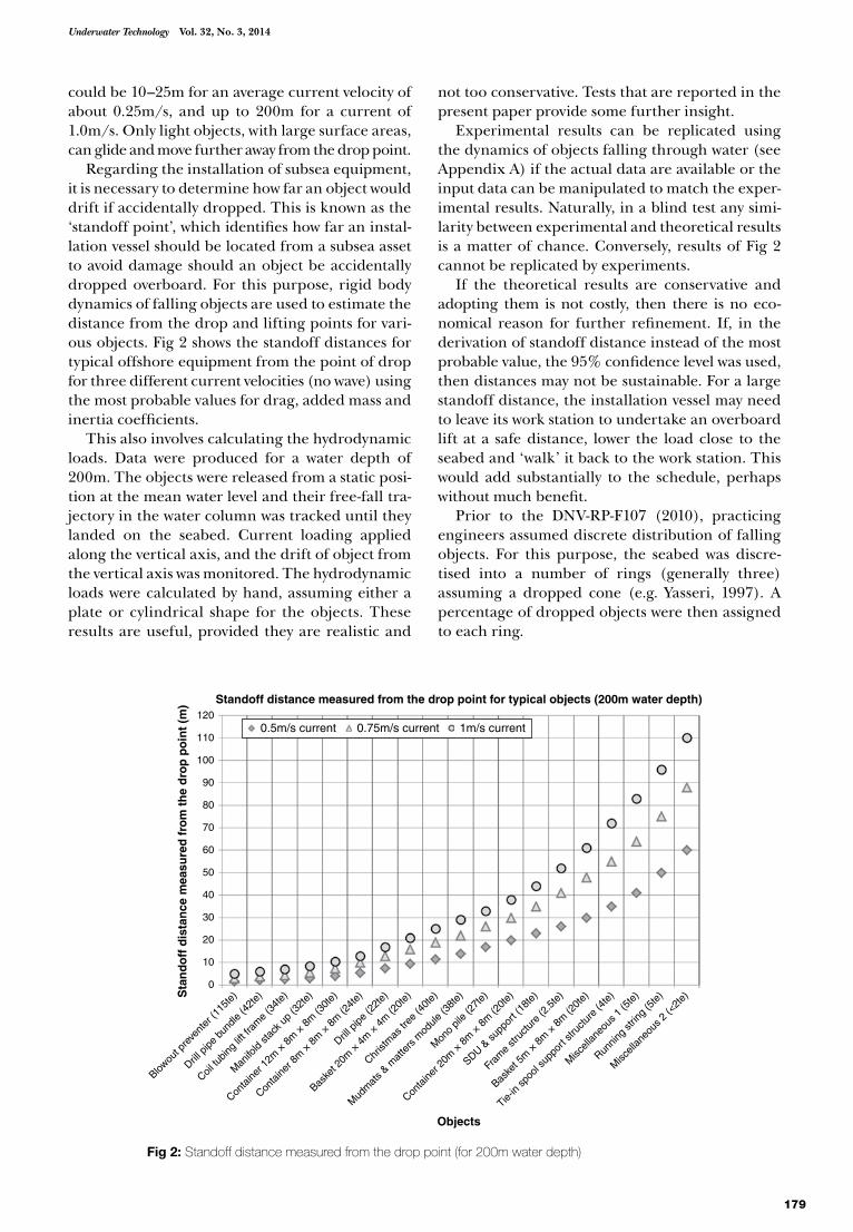
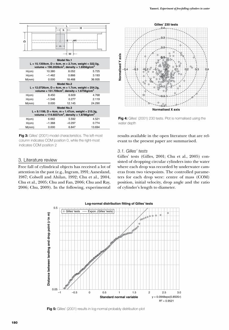
Yasseri Experiment of free-falling cylinders in water
180
3 Literature reviewFree fall of cylindrical objects has received a lot of attention in the past (eg Ingram 1991 Aanesland 1987 Colwell and Ahilan 1992 Chu et al 2004 Chu et al 2005 Chu and Fan 2006 Chu and Ray 2006 Chu 2009) In the following experimental
results available in the open literature that are rel-evant to the present paper are summarised
31 Gillesrsquo tests Gillesrsquo tests (Gilles 2001 Chu et al 2005) con-sisted of dropping circular cylinders into the water where each drop was recorded by underwater cam-eras from two viewpoints The controlled parame-ters for each drop were centre of mass (COM) position initial velocity drop angle and the ratio of cylinderrsquos length to diameter
05
Log-normal distribution fitting of Gillesrsquo tests
005
Dis
tan
ce b
etw
een
lan
din
g a
nd
dro
p p
oin
t (r
in m
)
ndash1 ndash05 05 1
Standard normal variable
15 2 25
R2 = 09521
y = 00948epx(08505r )
300
Expon (Gillesrsquo tests)Gillesrsquo tests
Fig 5 Gillesrsquo (2001) results in log-normal probably distribution plot
Fig 3 Gillesrsquo (2001) model characteristics The left-most column indicates COM position 0 while the right-most indicates COM position 2
Model No1L = 151359cm D = 4cm m = 27cm weight = 3225g
volume = 1902028cm3 density = 16956gcm3
H(cm) 10380 8052 5725
H(cm) ndash1462 0866 3193
M(mm) 0000 18468 36935
Model No2L = 120726cm D = 4cm m = 17cm weight = 2542g
volume = 151709cm3 density = 16756gcm3
H(cm) 8450 6609 4768
H(cm) ndash1546 0277 2119
M(mm) 0000 12145 24290
Model No3L = 91199 D = 4cm m = 147cm weight = 2153g
volume = 1146037cm3 density = 18786gcm3
H(cm) 6662 5592 4521
H(cm) ndash1368 ndash0297 0774
M(mm) 0000 6847 13694
Fig 4 Gillesrsquo (2001) 230 tests Plot is normalised using the water depth
Gillesrsquo 230 tests
Normalised X axis
No
rmal
ised
Y a
xis
04
03
02
01
ndash01
ndash01 01 02 03 04ndash02ndash03ndash04
ndash02
ndash03
ndash04
00
181
Underwater Technology Vol 32 No 3 2014
Fig 6 Shapes used by Ray (2006)
Rayrsquos models (2006)L
(cm)D
(cm)Mass
(g)COM(cm)
Density(gcm3)
Numberof tests
3185 483 5634 1375 2224 8
2794 402 473 142 2224 12
3175 518 831 1585 1754 11
3175 518 808 1610 1754 11
Bomb
Shell
Cylinder
Capsule
COM
COM
COM
COM
L
L
L
L
D
D
D
D
Gilles used three cylindrical shapes which had a circular diameter of 4cm however the lengths were about 15cm 12cm and 9cm respectively The bod-ies were constructed of rigid plastic with aluminium-capped ends Inside each was a threaded bolt running lengthwise across the model and an inter-nal weight The internal weight was used to vary the COM (see Fig 3) The drop angles were 15deg 30deg 45deg 60deg and 75deg This range produced velocities whose horizontal and vertical components varied in mag-nitude and allowed for comparison of trajectory sensitivity with the varying velocity components Gilles (2001) reported results for 230 tests
Gilles (2001) used five COM positions For posi-tive COM cases the COM was located below the centre of buoyancy For negative cases the COM was located above the centre of buoyancy prior to release Fig 4 shows Gillesrsquo results in normalised form The x and y coordinates were normalised by dividing them by the poolrsquos depth Circles of 10 20 30 and 40 of water depth are superim-posed on Fig 4
According to Gillesrsquo experiment 80 of objects landed within 20 of the water depth Almost 99 of objects landed within 40 of the water depth which clearly indicates a non-normal distribution contrary to the DNV assumption Fig 5 shows these results on a lognormal probability plot Appendix B shows how to determine the lognormal distribution parameters using the experimental data Direction-ality seen in Fig 4 is owing to the experimental setup All tests were done at one corner of the pool
Gilles (2001) grouped his tests into six series with the differentiating factor between the series being the drop angle However no discernible
correlation was found between the landing point and the drop angle although vertical drops were more likely to land closer to the point of drop
32 Rayrsquos testsRay (2006) used four polyester resin shapes for his experiments He reported 42 experiments using various shapes as shown in Fig 6 Dimensions of Rayrsquos model are also noted in Fig 6
The cylinder is the most predictable and stable shape of all (Ray 2006) Out of a total of 11 test runs
Fig 7 Landing point for Rayrsquos (2006) tests (42 points)
Rayrsquos tests (42 points)
Normalised X axis
No
rmal
ised
Y a
xis
05
04
03
02
01
ndash01
ndash02
ndash03
ndash04
ndash05
00 01ndash01ndash02ndash03ndash04ndash05 02 03 04 05
Capsule Shell Bomb Cylinder
Yasseri Experiment of free-falling cylinders in water
182
nine of the shapes exhibited an almost vertical trajectory pattern from the point of water entry to the landing point Models were launched orthogo-nal to the waterrsquos surface with initial velocities ranging from 28ms to 67ms The upper bound of velocity in offshore applications when an object hits the surface of the water is about 15ms
Fig 7 shows the landing points for all Rayrsquos 31 exp -eriments normalised using the water depth Owing to vertical entry all impact points for cylinders are within 105 of water depth Despite the high veloc-ity and nominal vertical entry impact points are somewhat away from the projection of entry point on the poolrsquos bottom Similar observations were made
Fig 8 Details of Allenrsquos (2006) models
Model Shape Dimensions (cm)No oftests
Model1
D 130Scale NA
Distance fromCOM to COV = 0
13
Model2
D 149H 133
Scale NADistance from
COM to COV = 0
9
Model3
D 150H 70Scale
COM to COV =+0373
along Z axis
15
Model4
L 160W(Back) 78
W(Front) 133H(Back) 63H(Front) 38
Scale 16COM to COV = 0
14
Mass ndash 16920gDensity ndash 1335gcm3
Mass ndash 28150gDensity ndash 1722gcm3
Mass ndash 11450gDensity ndash 1615gcm3
Mass ndash 8130gDensity ndash 1388gcm3
65cm
130cmCOM
55cm
133cm
149cm
745cm
62cm
75cm
38cm63cm
32cm
82cm
55cm
78cm133cm
160cm
16cm
70cm
150cm
COM
COM
COM
COM
COM
COM
183
Underwater Technology Vol 32 No 3 2014
by Bushnell (2001) where he fired missiles at 380ms into a pond from a nominal vertical direction
33 Allenrsquos testsAllen (2006) experimented with small samples in a 25m-deep pool using four shapes These shapes are shown in Fig 8 The model included a sphere that is symmetric and has equal weight distribution about its three axes
Fig 9 shows the landing point for all shapes in Allenrsquos tests Again the same pattern emerges ie dispersion clustering within 20 of the depth Some of the hemi-spherical shapes landed beyond this limit However no excursion extended beyond 50 of the depth and the largest excursion was for flat-shape objects Allenrsquos (2006) results also follow a lognormal distribution
Bushnell (2001) fired missiles into a pond at high velocity (about 300ms) at angles of attack between 1 and 35deg In addition the test specimen had tail fins some of which broke during the test In Bushnellrsquos test most missiles hit the pond floor within a circle of 02 of the water depth Bushnell experimented with missiles at a high velocity through the water where flow separation creates a cavity of air around the body That cavity is also called cavi-tation which remains in the water long after the missile has passed to influence the trajectory
4 Current model testsThe authorrsquos experiments consisted of dropping three cylindrical models of various lengths and
COM location into a 25m-deep pool at low veloc-ity similar to Gillesrsquo models (2001) (see Fig 10) The entry of each model into the water was recorded by the surface experimenter A mat with gridlines was placed on the poolrsquos bottom to facilitate the record-ing of the landing points All models were num-bered as well as marked with bright colours for ease of detection
The testing was conducted by two experiment-ers One experimenter remained at the surface and was responsible for launching the models and record-ing all test data The other experimenter was inside the pool with breathing apparatus and reported the landing point and the observed trajectory to the surface experimenter for recoding No test was dis-carded However prior to the commencement of the actual testing several trial runs were attempted in order to eliminate all likely problems This trial run also provided a procedure for performing the tests No underwater cameras were used to record the trajectory of the dropped cylinders
The controlled parameters were the cylindersrsquo physical parameters (length-to-diameter ratio COM) and initial drop conditions (initial velocity and drop angle) The models were based on the assumption that a 9m tubular is dropped in 180m of water thus producing a 201 ratio The depth of the pool was ~25m From this ratio 12cm was chosen for the length of the model Two additional models 9cm and 15cm in length were also used
Fig 10 The current model
L
δ
dCOV COM
C o G of extra mass
x
Fig 11 Schematic of experimental setup
WeightEntry point
Φ
Distance toCOM
~ 25mdepth
Fig 9 Allenrsquos (2006) tests Plot is normalised using the water depth
Allenrsquos tests (51 points)
Normalised X axis
No
rmal
ised
Y a
xis
04
03
02
01
ndash01
ndash01 01 02 03 04ndash02ndash03ndash04
ndash02
ndash03
ndash04
00
Sphere-Model 1(Fig 8)
Hemisphere-Model 2(Fig 8)
Model 3 (Fig 8) Model 4 (Fig 8)
Yasseri Experiment of free-falling cylinders in water
184
for the sensitivity analysis The outer radius of all the models was 4cm
The models were constructed of rigid plastic with a cap at both ends Fig 11 shows a schematic of the experimental setup A mass was inserted inside the model (Fig 11) to vary the COM for each model A total of nine models with three different lengths and three centres of mass for each length were pro-duced Owing to symmetry by turning the models around the COM can be below or above the centre of buoyancy
After dropping all nine models the experimenter inside the pool reported the results and recovered the models The surface experimenter then signalled his readiness for the next nine tests This cycle then was repeated until all the tests for a given drop angle were concluded
The initial orientation of the drop can be set between 0deg and 90deg with 0deg being a vertical initial orientation and 90deg being horizontal Drop angles were 15deg 30deg 45deg 60deg and 75deg This produces a situa-tion where the cylinder is heading directly down-ward throughout the event If an object dropped vertically even with no initial rotation the object will still tend to acquire a horizontal velocity component as it falls through the water This results in the object impacting the seabed at a random angle and loca-tion Several trajectory patterns (straight spiral flip flat seesaw and combination) were observed during the experiment but the four patterns as shown in Fig 12 were more frequent The COM position had the largest influence on the trajectory of cylinders
The drop point scatter plot is shown in Fig 13 When the COMs and buoyancy coincided objects
Fig 12 More frequent trajectory patterns of falling cylinders (see also Chu et al 2005)
Arc trajectory Straight trajectory
Early flip Late flip
X or Y
Wat
er d
epth
(Z
)
ndash15 ndash1 ndash05 00
ndash05
ndash1
ndash15
ndash2
ndash25
05 1 15
X or Y
Wat
er d
epth
(Z
)
ndash15 ndash1 ndash05 00
ndash05
ndash1
ndash15
ndash2
ndash25
05 1 15
X or Y
Wat
er d
epth
(Z
)
ndash15 ndash1 ndash05 00
ndash05
ndash1
ndash15
ndash2
ndash25
05 1 15
X or Y
Wat
er d
epth
(Z
)
ndash15 ndash1 ndash05 00
ndash05
ndash1
ndash15
ndash2
ndash25
05 1 15
185
Underwater Technology Vol 32 No 3 2014
fell near the drop point for more than 90 of the time while a small distance between COM and the centre of volume (COV) caused the variability When the centre of buoyancy is ahead of the COM
the model flips while descending and experi-enced the largest excursion from the drop point When the drop angle is close to 90o and the centre of buoyancy and COM coincide then the descent is mostly vertical with only a slight slant When the buoyancy centre is above the mass centre models approach the floor at acute angles between 120deg and 180deg The trajectory patterns of each model type are affected by the size and shape of the mod-els The four generalised patterns were not shared among the various shapes but rather they were quite consistent within each shape type
Fig 14 shows the distance between the landing point and drop point in a lognormal probability plot It can be seen that the lognormal distribu-tion describes the probability of the landing spot fairly well Fig 15 shows results from another set of experiments where a cylinder with a length of 10cm and diameter of 12cm and a cube of 15cm times 15cm times 15cm were dropped using the same experimental setup These 140 points also follow a lognormal distbution similar to Fig 14 Fig 16 shows a few of the observed trajectories of the falling cylinder and cube in the second set of experiments
Fig 14 Authorrsquos results on a lognormal probability plot (324 points)
Probability plot of landing points for the current tests (324 points)
Standard normal variable
Dis
tan
ce b
etw
een
lan
din
g p
oin
t an
d t
he
dro
p p
oin
t
ndash3 ndash25 ndash2 ndash15 ndash1 ndash05 0 0505
005y = 01033exp(08147r)
R2 = 09828
Experimental dataExpon (Experimental data)
1 15 2 25 3
Fig 13 A plot of the landing point of all authorrsquos 324 tests
Landing points of 324 model cylinders droppedinto 25m of water
No
rmal
ised
Y a
xis
Normalised X axis
04
03
02
01
01 02 03 040
0
ndash01
ndash02
ndash03
ndash04
ndash04 ndash03 ndash02 ndash01
Yasseri Experiment of free-falling cylinders in water
186
5 Computational approachThe motion of three-dimensional rigid bodies freely falling through water has been addressed by many researchers Appendix A outlines the formu-lation necessary to track such motion MATLAB commercial software was used to solve these equa-tions Owing to a rigid body assumption tracking of one point gives enough data to plot the position of the falling object (Fig 17) Fig 18 shows some examples of trajectories using different values of control variables
These equations replicate the experimental results fairly well The method is applied to cylin-drical bodies initially released below the free sur-face in calm water Depending on the initial body orientation body aspect ratio and mass distribu-tion it is possible to identify key characteristic pat-terns of the body motion which compare remarkably with observations in the tank-drop tests The present study has a significant implica-tion to the manoeuvring of underwater vehicles Abelev et al (2007) presented experimental results of falling heavy cylindrical shapes which are in line with the authorrsquos results
6 Concluding remarksNot all falling objects travel straight downward under the influence of gravity even in the air Sometimes the falling objects follow complicated downward trajectories as they fall It is therefore
clear that any satisfactory explanation of this com-plex phenomenon must include a description of the instantaneous fluid forces experienced by the falling object as well as the inertial and gravita-tional effects that are present
Fig 16 A few of the observed trajectories for the second set of tests
Fig 17 Tracking the orientation of a falling object with position of COM lower than COV
Trajectory of a cylindrical object with heavy nose
10
0
ndash10
ndash20
ndash30
Wat
er d
epth
(m
)
Horizontal position (m)
ndash40
ndash50
ndash60
ndash70
ndash80ndash10 0 10 20 30 40 50 60 70 80
Nose position
Fig 15 Scatter plot for two shapes a short cylinder with lengthdiameter lt 1 and a small cube (140 points)
Landing points for dropped short cylinder anda cube of 150cm times 150cm times 150cm
04
03
02
01
ndash01
ndash02
ndash03
ndash04
ndash04 ndash03 ndash02 ndash01 0 01 02 03 04
Normalised X axis
No
rmal
ised
Y a
xis
0
Cylinder Drop point Box-shape
187
Underwater Technology Vol 32 No 3 2014
The entry of a solid into water or other liquids gives rise to a sequence of complex events The evolution of the air cavity behind the falling body after the initial impact significantly influences the dynamics and trajectory of low-speed projectiles (see eg Chu and Fan 2006 Chu and Ray 2006) The effect of air cavity dynamics is more pro-nounced in large body water entry Leaves tree seeds and paper cards falling in air are spectacular examples of time-dependent fluid dynamics at intermediate Reynolds numbers at which both inertial and viscous effects are important The tra-jectory of a falling card typically appears to be very complex with the card either oscillating from side to side (fluttering) or rotating and drifting side-ways (tumbling)
It is acknowledged that there are deficiencies in representing the landing point using a statistical distribution Fitting a distribution to a set of data only tells us how the dispersion would look The data behind the DNV recommendation (2010)
could not be located which makes the compari-sons between the DNV recommendation and the current experiment difficult In addition the log-normal curve may not represent the effect of all input parameters adequately It was chosen as the first approximation with an overall goal of developing a stochastic model evaluation Other distributions may be examined and could poten-tially represent the experimentally measured data better
Real objects of any significance are generally longer than 6m but still much smaller than the water depth for deepwater locations Thus the ratio of water depth to the object length is quite high Hence replicating it in a model test requires a very small model if the pool is not very deep It is desir-able that the choice of scale is representative of the offshore industryrsquos ratio of water depth to object length but at the same time it should be large enough to cover typical offshore tubular sizes The ratio of water depth to the tubular length for a
Fig 18 A few calculated trajectories for a falling cylinder with different orientation initial velocity and hydrodynamic conditions
Yasseri Experiment of free-falling cylinders in water
188
dropped tubular model of 12m in length in a water depth of 240m is 20 Therefore for a pool depth of 25m the model length should be around 120mm
Ingram (1991) surmises there is a depth beyond which an object would fall flat implying there is a single pattern in deep water However no single pattern was observed in these tests
Pulling together all tests reported here the fol-lowing observations can be made about the land-ing location of free-falling cylinders
bullAbout 50 of the time objects land within 10 of the water depth
bullAbout 80 of the time objects land within 20 of the water depth
bullAbout 90 of the time objects land within 30 of water depth
bullAbout 95 of the time objects land within 40 of water depth
bullAbout 98 of the time objects land within 50 of water depth
These tests were performed in pools where the water surface only experiences small ripples However there is significantly more undulation in the ocean surface Such undulation will cause more deviation to the object and help it to travel further (Fig 19)
ReferencesAanesland V (1987) Numerical and experimental investi-
gation of accidentally falling drilling pipes OTC 5494 19th Offshore Technology Conference April 1987 Houston USA
Abelev AV Valent PJ and Holland KT (2007) Behaviour of a large cylinder in free fall through water IEEE Journal of Ocean Engineering 32 10ndash20
Allen CR (2006) Mine drop experiment II with operational mines shapes (MIDEX II) MS Thesis Naval Postgraduate School Monterey CA USA 306pp Available at httpfacultynpsedupcchuweb_paperthesis06Mar_Allenpdf last accessed lt14 September 2014gt
Bushnell JM (2001) Tail separation and density effects on the underwater trajectory of the JDAM MS Thesis Naval Postgraduate School Monterey CA USA 88pp Available at httpcalhounnpsedupublichandle109454406 last accessed lt14 September 2014gt
Chu PC (2009) Mine impact burial prediction from one to three dimensions ASME Journal of Applied Mechanics Review 62
Chu PC and Fan CW (2006) Prediction of falling cylinder through air-water-sediment columns ASME Journal of Applied Mechanics Review 73 300ndash314
Chu PC and Ray G (2006) Prediction of high speed rigid body manoeuvring in air-water-sediment columns In Rahman M and Brebbia CA (eds) Advances in Fluid Mechanics V Southampton UK WIT Press 123ndash132
Chu PC Fan CW Evans AD and Gilles AF (2004) Triple coordinate transforms for prediction of falling cylinder through the water column Journal of Applied Mechanics 71 292ndash298
Chu PC Gilles AF and Fan CW (2005) Experiment of falling cylinder through the water column Experimental Thermal and Fluid Science 29 555ndash568
Colwill RD and Ahilan RV (1992) Reliability analysis of the behaviour of dropped objects OTC 6918 24th Offshore Technology Conference April 1992 Houston USA
Det Norske Veritas (DNV) (2010) Risk assessment of pipeline protection Recommended practice No DNV-RP- F107 Olso Norway DNV 45pp
Evans A (2002) Hydrodynamics of mine impact burial MS Thesis Naval Postgraduate School Monterey CA 2002 Available at httpcalhounnpseduhandle10945 5310show=full last accessed lt14 September 2014gt
Friedman A Zilman G and Miloh T (2003) Dynamics of a body falling in waves In Proceedings of 18th Interna-tional Workshop of Water Waves and Floating Bodies (IWWWFB) Ann Arbour MI USA
Gilles A (2001) Mine Drop Experiment (MIDEX) MS The-sis Naval Postgraduate School Monterey CA USA 446pp Available at httpfacultynpsedupcchuweb_paperthesisgillespdf last accessed lt14 September 2014gt
Ingram JG (1991) Experimental modelling and risk assess-ment of dropped offshore tubulars MS Thesis School of Industrial and Manufacturing Science Cranfield Insti-tute of Technology Cranfield UK
Kim Y Lin KY and Yue KD (2002) Motion dynamics of three-dimensional bodies falling through water In Rainey RCT and Lee SF (eds) Proceedings of 17th International Workshop of Water Waves and Floating Bodies (IWWWFB) London WS Atkins Consultants 81ndash84 Available at httpwwwiwwwfborgAbstractsiwwwfb17iwwwfb17_21pdf last accessed lt14 September 2014gt
Ray G (2006) Bomb strike experiments for mine counter-measure MS Thesis Naval Postgraduate School Monte-rey CA USA 197pp Available at httpfacultynpsedupcchuweb_paperthesis06Mar_Raypdf last accessed lt14 September 2014gt
Von Mises R (1959) Theory of Flight 1st edition New York Dover Publications Inc 629pp
Wierzbicki T and Yue DK (1986) Impact damage of Chal-lenger crew compartment Journal of Spacecraft and Rockets 23 646ndash654
Yasseri S (1997) Risk-based decision analysis for the protec-tion of marine pipelines from dropped objects In Proceed-ings of 7th International Offshore and Polar Engineering Conference Honolulu USA 251ndash256
Fig 19 The effect of undulating sea surface on the trajectory and drifting
Drift owing to object hitting the wave atdifferent location
Wave slope
Entry angle
189
Underwater Technology Vol 32 No 3 2014
Appendix A
Rigid body dynamics of a cylinder falling through waterThere are various methods of describing the motion of a rigid body see for example Von Mises (1959) Chu et al (2005) Wierzbicki and Yue (1986) Kim et al (2002) and Friedman et al (2003) In the fol-lowing equations which are needed to track the dynamics of motion of three-dimensional rigid bod-ies falling through water (Chu et al 2005) are given
Fig 20 shows a right circular symmetric cylinder whose centres of mass (X) and volume (B) are on the cylinderrsquos longitudinal axis Parameters (L d x) denote the cylinderrsquos length diameter and the dis-tance between the two points (X B) The positive case is when the centre of mass (COM) is lower than the centre of volume (COV) ie x is positive (Evans 2002)
Three orthogonal right-handed coordinate sys-tems (Fig 21) are used describe the dynamics of a falling cylinder through the water which are E-coordinate M-coordinate and F-coordinate sys-tems The body and buoyancy forces and their moments are given in the E-coordinate system the hydrodynamic forces (drag lift and inertia forces) and their moments are given in the F-coordinate and the cylinderrsquos moments of gyration are given in the M-coordinate The E-coordinate system is fixed to the Earthrsquos surface with horizontal sides as x and y axes are parallel with the Earthrsquos surface (along the two sides of the pool) and vertical direc-tion as z axis (upward positive Fig 20)
Suppose the cylinder is falling into the water The cylinder rotates around its main axis (r1) with an angle ψ1 and an angular velocity of Ω Its position
is represented by the COM and its orientation is represented by two angles ψ2 and ψ3 (Fig 3) Here ψ2 is the angle between the r1 axis and the horizon-tal plane and ψ3 is the angle between the projec-tion of the main axis in the (x y) plane and the x axis The angle (ψ2 + π2) is usually called attitude
The relative coordinate is rigidly connected with the cylinder The origin (O) of the relative coordi-nate system coincides with the COM the r1 axis is along the central line of the cylinder the r2 axis is perpendicular to the plane constructed by r1 axis and z-axis (r1-z plane) and the r3-axis lies in the (r1-z) plane and is perpendicular to r1 axis The axes (x y z) and (r1 r2 r3) follows the right-hand rule
Let V = (V1 V2 V3 ) the three components of the velocity of COM ie the origin velocity of the coor-dinate system (r1 r2 r3) The geometric centre (GC) is located at (x 0 0) if for GC below COM x gt 0 and for GC above COM x lt 0 The relative coordinate system (r1 r2 r3) is obtained by one translation and two rotations ψ2 and ψ3 of the E-coordinate system Let the position vector (P) be represented by PE and
Fig 20 M-coordinate with the COM as the origin X (im jm) x is the distance between the COV (B) and COM (X) L and d are the cylinderrsquos length and diameter (Chu et al 2005)
2
d
L2L
B
xjm
imX
z (k )
y ( j )
kmjmψ2
imo ψ3
x (i )
obull
kf
jf
ifobull
V1
V2 Vr
Fig 21 Cylinder orientation and relative coordinate system
Yasseri Experiment of free-falling cylinders in water
190
PB in the Earth and relative coordinate systems PE and PB are connected by
PE =minus
minus
cos sin
sin cos
cos sin
si
ψ ψψ ψ
ψ ψ
3 3
3 3
2 2
0
0
0 0 1
0
0 1 0
nn cosψ ψ2 20
+
lowast
lowast
lowast
P
x
y
zB
m
m
m
(A1)
where (xm ym zm) represent the position of COM in the Earthrsquos coordinate system
The motion of a solid object falling through a fluid is governed by two principles (1) momentum balance and (2) moment of momentum balance Let Vw = (Vw1 Vw2 Vw3) be the water velocity and (ω1 ω2 ω3) be the components of the angular velocity referring to the direction of the relative coordinate system Variables are made non-dimensional by
tgL
tLg
VV
gL= = =lowast lowast
lowast
ω (A2)
where g is the gravitational acceleration and L the length of the cylinder The non-dimensional momentum equations for COM are given by (Van Mises 1959)
dVdt
V VFg
w12 3 3 2 2
1+ minus =minus
+forall
lowast
ω ωρ ρ
ρψ
ρsin (A3)
dVdt
VFg
23 1
2+ =forall
lowast
ωρ
(A4)
dVdt
VFg
w32 1 2
3minus =minus
+forall
lowast
ωρ ρ
ρψ
ρcos (A5)
where forall is the volume of the cylinder ρ is the cylinder density ρw is the water density and (F1
F2 F3
) are the components of fluid drag The non-dimensional equations of the moment of momentum for circu-lar symmetric cylinder are
ddt
J JJ
LMg J
Ω+
minus=
lowast3 2
12 3
1
1
ω ω (A6)
ddt
x LJ
LMg J
wω ρ ρψ2
22
2
2
= minusforall minus
+lowast lowast( )
cos (A7)
ddt
LMg J
ω3 3
3
=lowast
(A8)
where x is the distance between COM and GC and (M1
M2 M3
) are the components of the moment
owing to drag (J1 J2 J3) The three moments of gyration are
J r r dm J r r dm
J r r dm
1 22
32
2 32
12
3 12
22
= + = +
= +
int intint
lowast lowast
lowast
( ) ( )
( )and (A9)
The orientation of the cylinder (ψ2 ψ3) is deter-mined by
ddt
ddt
ψω ψ
ψω2
2 23
3= = cos (A10)
The eight non-dimensional nonlinear equations (A2 to A5) (A6 to A8) and (A10) are the funda-mental equations for determining the cylinder movement in the water
All the equations were solved using the 4th order Runge-Kutta scheme for integration with time in MATLAB At any instant the hydrody-namic loads were computed using a panel method
Appendix B
Probability plottingA method that may be used to visualise distri-butions and estimate parameters is probability plotting also referred to as linear least-squares regression or regression on ordered statistics This technique involves finding a probability and data scale that plots the cumulative distribution func-tion (CDF) of a hypothesised distribution as a straight line The corresponding linearity of the CDF for the sample data provides a measure of the goodness-of-fit of the hypothesised distribution
The n test results (ri r2hellip rn) were arranged in increasing order the mth value is marked on the verti-cal axis and corresponds to a cumulative probability of p = m(N + 1) marked on the horizontal axis Then the value of standardised normal variable for each p was calculated using the normal distribution table
The distance between the drop point and the landing point were ordered in terms of increasing magnitude in a table and the cumulative frequency of each ratio were determined which is equal to the cumulative probability of p For each p the value for the corresponding standard normally distributed variable is then calculated and noted in that table Samples of (Zi ri) are plotted on the logarithmic normal distribution graph as shown in Fig 14
The straight line equation that best fits the sam-ples can be written as
y = a e bx (B1)
where a and b are constants
191
Underwater Technology Vol 32 No 3 2014
Taking logarithm of both sides of this equation results in
lny = lnα + bx (B2)
The standard normal variable becomes
sr
rii s= = +minusln λ
ζλ ζ or ln (B3)
Equating two equations gives the ordinate inter-cept of the straight line and its slope ie
λ = lnα amp b = ζ (B4)
Then the mean value of landing points (r) is
r = rE = exp(λ + 05ζ2) (B5)
From Fig 14 it can be seen that they can be approximated by the following straight line
y = 01033e08147x (B6)
λ = ln(01033) = minus227012 ζ = b = 08147 (B7)
r = rE = exp(minus227012 + 05 times 081472)= 01439 (1439 of the water depth) (B8)
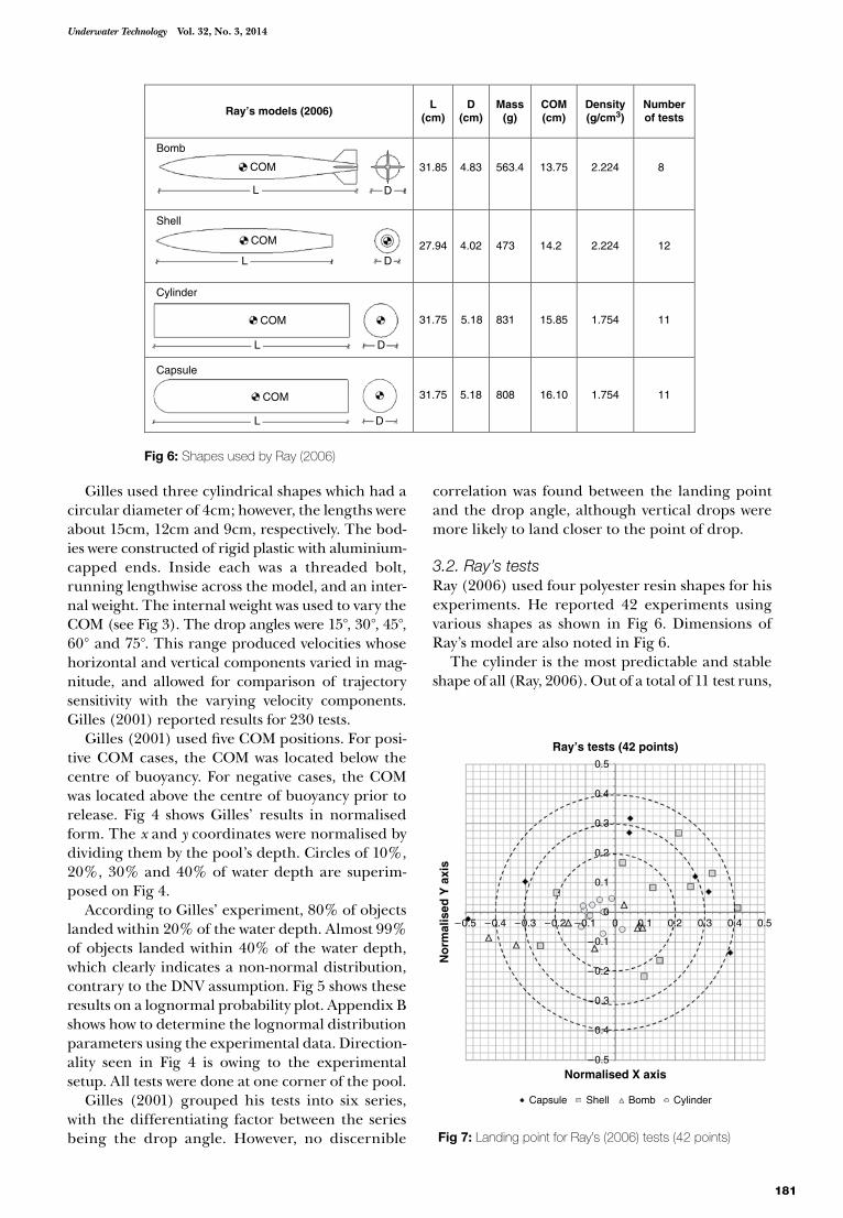
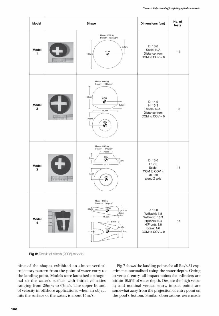
Yasseri Experiment of free-falling cylinders in water
182
nine of the shapes exhibited an almost vertical trajectory pattern from the point of water entry to the landing point Models were launched orthogo-nal to the waterrsquos surface with initial velocities ranging from 28ms to 67ms The upper bound of velocity in offshore applications when an object hits the surface of the water is about 15ms
Fig 7 shows the landing points for all Rayrsquos 31 exp -eriments normalised using the water depth Owing to vertical entry all impact points for cylinders are within 105 of water depth Despite the high veloc-ity and nominal vertical entry impact points are somewhat away from the projection of entry point on the poolrsquos bottom Similar observations were made
Fig 8 Details of Allenrsquos (2006) models
Model Shape Dimensions (cm)No oftests
Model1
D 130Scale NA
Distance fromCOM to COV = 0
13
Model2
D 149H 133
Scale NADistance from
COM to COV = 0
9
Model3
D 150H 70Scale
COM to COV =+0373
along Z axis
15
Model4
L 160W(Back) 78
W(Front) 133H(Back) 63H(Front) 38
Scale 16COM to COV = 0
14
Mass ndash 16920gDensity ndash 1335gcm3
Mass ndash 28150gDensity ndash 1722gcm3
Mass ndash 11450gDensity ndash 1615gcm3
Mass ndash 8130gDensity ndash 1388gcm3
65cm
130cmCOM
55cm
133cm
149cm
745cm
62cm
75cm
38cm63cm
32cm
82cm
55cm
78cm133cm
160cm
16cm
70cm
150cm
COM
COM
COM
COM
COM
COM
183
Underwater Technology Vol 32 No 3 2014
by Bushnell (2001) where he fired missiles at 380ms into a pond from a nominal vertical direction
33 Allenrsquos testsAllen (2006) experimented with small samples in a 25m-deep pool using four shapes These shapes are shown in Fig 8 The model included a sphere that is symmetric and has equal weight distribution about its three axes
Fig 9 shows the landing point for all shapes in Allenrsquos tests Again the same pattern emerges ie dispersion clustering within 20 of the depth Some of the hemi-spherical shapes landed beyond this limit However no excursion extended beyond 50 of the depth and the largest excursion was for flat-shape objects Allenrsquos (2006) results also follow a lognormal distribution
Bushnell (2001) fired missiles into a pond at high velocity (about 300ms) at angles of attack between 1 and 35deg In addition the test specimen had tail fins some of which broke during the test In Bushnellrsquos test most missiles hit the pond floor within a circle of 02 of the water depth Bushnell experimented with missiles at a high velocity through the water where flow separation creates a cavity of air around the body That cavity is also called cavi-tation which remains in the water long after the missile has passed to influence the trajectory
4 Current model testsThe authorrsquos experiments consisted of dropping three cylindrical models of various lengths and
COM location into a 25m-deep pool at low veloc-ity similar to Gillesrsquo models (2001) (see Fig 10) The entry of each model into the water was recorded by the surface experimenter A mat with gridlines was placed on the poolrsquos bottom to facilitate the record-ing of the landing points All models were num-bered as well as marked with bright colours for ease of detection
The testing was conducted by two experiment-ers One experimenter remained at the surface and was responsible for launching the models and record-ing all test data The other experimenter was inside the pool with breathing apparatus and reported the landing point and the observed trajectory to the surface experimenter for recoding No test was dis-carded However prior to the commencement of the actual testing several trial runs were attempted in order to eliminate all likely problems This trial run also provided a procedure for performing the tests No underwater cameras were used to record the trajectory of the dropped cylinders
The controlled parameters were the cylindersrsquo physical parameters (length-to-diameter ratio COM) and initial drop conditions (initial velocity and drop angle) The models were based on the assumption that a 9m tubular is dropped in 180m of water thus producing a 201 ratio The depth of the pool was ~25m From this ratio 12cm was chosen for the length of the model Two additional models 9cm and 15cm in length were also used
Fig 10 The current model
L
δ
dCOV COM
C o G of extra mass
x
Fig 11 Schematic of experimental setup
WeightEntry point
Φ
Distance toCOM
~ 25mdepth
Fig 9 Allenrsquos (2006) tests Plot is normalised using the water depth
Allenrsquos tests (51 points)
Normalised X axis
No
rmal
ised
Y a
xis
04
03
02
01
ndash01
ndash01 01 02 03 04ndash02ndash03ndash04
ndash02
ndash03
ndash04
00
Sphere-Model 1(Fig 8)
Hemisphere-Model 2(Fig 8)
Model 3 (Fig 8) Model 4 (Fig 8)
Yasseri Experiment of free-falling cylinders in water
184
for the sensitivity analysis The outer radius of all the models was 4cm
The models were constructed of rigid plastic with a cap at both ends Fig 11 shows a schematic of the experimental setup A mass was inserted inside the model (Fig 11) to vary the COM for each model A total of nine models with three different lengths and three centres of mass for each length were pro-duced Owing to symmetry by turning the models around the COM can be below or above the centre of buoyancy
After dropping all nine models the experimenter inside the pool reported the results and recovered the models The surface experimenter then signalled his readiness for the next nine tests This cycle then was repeated until all the tests for a given drop angle were concluded
The initial orientation of the drop can be set between 0deg and 90deg with 0deg being a vertical initial orientation and 90deg being horizontal Drop angles were 15deg 30deg 45deg 60deg and 75deg This produces a situa-tion where the cylinder is heading directly down-ward throughout the event If an object dropped vertically even with no initial rotation the object will still tend to acquire a horizontal velocity component as it falls through the water This results in the object impacting the seabed at a random angle and loca-tion Several trajectory patterns (straight spiral flip flat seesaw and combination) were observed during the experiment but the four patterns as shown in Fig 12 were more frequent The COM position had the largest influence on the trajectory of cylinders
The drop point scatter plot is shown in Fig 13 When the COMs and buoyancy coincided objects
Fig 12 More frequent trajectory patterns of falling cylinders (see also Chu et al 2005)
Arc trajectory Straight trajectory
Early flip Late flip
X or Y
Wat
er d
epth
(Z
)
ndash15 ndash1 ndash05 00
ndash05
ndash1
ndash15
ndash2
ndash25
05 1 15
X or Y
Wat
er d
epth
(Z
)
ndash15 ndash1 ndash05 00
ndash05
ndash1
ndash15
ndash2
ndash25
05 1 15
X or Y
Wat
er d
epth
(Z
)
ndash15 ndash1 ndash05 00
ndash05
ndash1
ndash15
ndash2
ndash25
05 1 15
X or Y
Wat
er d
epth
(Z
)
ndash15 ndash1 ndash05 00
ndash05
ndash1
ndash15
ndash2
ndash25
05 1 15
185
Underwater Technology Vol 32 No 3 2014
fell near the drop point for more than 90 of the time while a small distance between COM and the centre of volume (COV) caused the variability When the centre of buoyancy is ahead of the COM
the model flips while descending and experi-enced the largest excursion from the drop point When the drop angle is close to 90o and the centre of buoyancy and COM coincide then the descent is mostly vertical with only a slight slant When the buoyancy centre is above the mass centre models approach the floor at acute angles between 120deg and 180deg The trajectory patterns of each model type are affected by the size and shape of the mod-els The four generalised patterns were not shared among the various shapes but rather they were quite consistent within each shape type
Fig 14 shows the distance between the landing point and drop point in a lognormal probability plot It can be seen that the lognormal distribu-tion describes the probability of the landing spot fairly well Fig 15 shows results from another set of experiments where a cylinder with a length of 10cm and diameter of 12cm and a cube of 15cm times 15cm times 15cm were dropped using the same experimental setup These 140 points also follow a lognormal distbution similar to Fig 14 Fig 16 shows a few of the observed trajectories of the falling cylinder and cube in the second set of experiments
Fig 14 Authorrsquos results on a lognormal probability plot (324 points)
Probability plot of landing points for the current tests (324 points)
Standard normal variable
Dis
tan
ce b
etw
een
lan
din
g p
oin
t an
d t
he
dro
p p
oin
t
ndash3 ndash25 ndash2 ndash15 ndash1 ndash05 0 0505
005y = 01033exp(08147r)
R2 = 09828
Experimental dataExpon (Experimental data)
1 15 2 25 3
Fig 13 A plot of the landing point of all authorrsquos 324 tests
Landing points of 324 model cylinders droppedinto 25m of water
No
rmal
ised
Y a
xis
Normalised X axis
04
03
02
01
01 02 03 040
0
ndash01
ndash02
ndash03
ndash04
ndash04 ndash03 ndash02 ndash01
Yasseri Experiment of free-falling cylinders in water
186
5 Computational approachThe motion of three-dimensional rigid bodies freely falling through water has been addressed by many researchers Appendix A outlines the formu-lation necessary to track such motion MATLAB commercial software was used to solve these equa-tions Owing to a rigid body assumption tracking of one point gives enough data to plot the position of the falling object (Fig 17) Fig 18 shows some examples of trajectories using different values of control variables
These equations replicate the experimental results fairly well The method is applied to cylin-drical bodies initially released below the free sur-face in calm water Depending on the initial body orientation body aspect ratio and mass distribu-tion it is possible to identify key characteristic pat-terns of the body motion which compare remarkably with observations in the tank-drop tests The present study has a significant implica-tion to the manoeuvring of underwater vehicles Abelev et al (2007) presented experimental results of falling heavy cylindrical shapes which are in line with the authorrsquos results
6 Concluding remarksNot all falling objects travel straight downward under the influence of gravity even in the air Sometimes the falling objects follow complicated downward trajectories as they fall It is therefore
clear that any satisfactory explanation of this com-plex phenomenon must include a description of the instantaneous fluid forces experienced by the falling object as well as the inertial and gravita-tional effects that are present
Fig 16 A few of the observed trajectories for the second set of tests
Fig 17 Tracking the orientation of a falling object with position of COM lower than COV
Trajectory of a cylindrical object with heavy nose
10
0
ndash10
ndash20
ndash30
Wat
er d
epth
(m
)
Horizontal position (m)
ndash40
ndash50
ndash60
ndash70
ndash80ndash10 0 10 20 30 40 50 60 70 80
Nose position
Fig 15 Scatter plot for two shapes a short cylinder with lengthdiameter lt 1 and a small cube (140 points)
Landing points for dropped short cylinder anda cube of 150cm times 150cm times 150cm
04
03
02
01
ndash01
ndash02
ndash03
ndash04
ndash04 ndash03 ndash02 ndash01 0 01 02 03 04
Normalised X axis
No
rmal
ised
Y a
xis
0
Cylinder Drop point Box-shape
187
Underwater Technology Vol 32 No 3 2014
The entry of a solid into water or other liquids gives rise to a sequence of complex events The evolution of the air cavity behind the falling body after the initial impact significantly influences the dynamics and trajectory of low-speed projectiles (see eg Chu and Fan 2006 Chu and Ray 2006) The effect of air cavity dynamics is more pro-nounced in large body water entry Leaves tree seeds and paper cards falling in air are spectacular examples of time-dependent fluid dynamics at intermediate Reynolds numbers at which both inertial and viscous effects are important The tra-jectory of a falling card typically appears to be very complex with the card either oscillating from side to side (fluttering) or rotating and drifting side-ways (tumbling)
It is acknowledged that there are deficiencies in representing the landing point using a statistical distribution Fitting a distribution to a set of data only tells us how the dispersion would look The data behind the DNV recommendation (2010)
could not be located which makes the compari-sons between the DNV recommendation and the current experiment difficult In addition the log-normal curve may not represent the effect of all input parameters adequately It was chosen as the first approximation with an overall goal of developing a stochastic model evaluation Other distributions may be examined and could poten-tially represent the experimentally measured data better
Real objects of any significance are generally longer than 6m but still much smaller than the water depth for deepwater locations Thus the ratio of water depth to the object length is quite high Hence replicating it in a model test requires a very small model if the pool is not very deep It is desir-able that the choice of scale is representative of the offshore industryrsquos ratio of water depth to object length but at the same time it should be large enough to cover typical offshore tubular sizes The ratio of water depth to the tubular length for a
Fig 18 A few calculated trajectories for a falling cylinder with different orientation initial velocity and hydrodynamic conditions
Yasseri Experiment of free-falling cylinders in water
188
dropped tubular model of 12m in length in a water depth of 240m is 20 Therefore for a pool depth of 25m the model length should be around 120mm
Ingram (1991) surmises there is a depth beyond which an object would fall flat implying there is a single pattern in deep water However no single pattern was observed in these tests
Pulling together all tests reported here the fol-lowing observations can be made about the land-ing location of free-falling cylinders
bullAbout 50 of the time objects land within 10 of the water depth
bullAbout 80 of the time objects land within 20 of the water depth
bullAbout 90 of the time objects land within 30 of water depth
bullAbout 95 of the time objects land within 40 of water depth
bullAbout 98 of the time objects land within 50 of water depth
These tests were performed in pools where the water surface only experiences small ripples However there is significantly more undulation in the ocean surface Such undulation will cause more deviation to the object and help it to travel further (Fig 19)
ReferencesAanesland V (1987) Numerical and experimental investi-
gation of accidentally falling drilling pipes OTC 5494 19th Offshore Technology Conference April 1987 Houston USA
Abelev AV Valent PJ and Holland KT (2007) Behaviour of a large cylinder in free fall through water IEEE Journal of Ocean Engineering 32 10ndash20
Allen CR (2006) Mine drop experiment II with operational mines shapes (MIDEX II) MS Thesis Naval Postgraduate School Monterey CA USA 306pp Available at httpfacultynpsedupcchuweb_paperthesis06Mar_Allenpdf last accessed lt14 September 2014gt
Bushnell JM (2001) Tail separation and density effects on the underwater trajectory of the JDAM MS Thesis Naval Postgraduate School Monterey CA USA 88pp Available at httpcalhounnpsedupublichandle109454406 last accessed lt14 September 2014gt
Chu PC (2009) Mine impact burial prediction from one to three dimensions ASME Journal of Applied Mechanics Review 62
Chu PC and Fan CW (2006) Prediction of falling cylinder through air-water-sediment columns ASME Journal of Applied Mechanics Review 73 300ndash314
Chu PC and Ray G (2006) Prediction of high speed rigid body manoeuvring in air-water-sediment columns In Rahman M and Brebbia CA (eds) Advances in Fluid Mechanics V Southampton UK WIT Press 123ndash132
Chu PC Fan CW Evans AD and Gilles AF (2004) Triple coordinate transforms for prediction of falling cylinder through the water column Journal of Applied Mechanics 71 292ndash298
Chu PC Gilles AF and Fan CW (2005) Experiment of falling cylinder through the water column Experimental Thermal and Fluid Science 29 555ndash568
Colwill RD and Ahilan RV (1992) Reliability analysis of the behaviour of dropped objects OTC 6918 24th Offshore Technology Conference April 1992 Houston USA
Det Norske Veritas (DNV) (2010) Risk assessment of pipeline protection Recommended practice No DNV-RP- F107 Olso Norway DNV 45pp
Evans A (2002) Hydrodynamics of mine impact burial MS Thesis Naval Postgraduate School Monterey CA 2002 Available at httpcalhounnpseduhandle10945 5310show=full last accessed lt14 September 2014gt
Friedman A Zilman G and Miloh T (2003) Dynamics of a body falling in waves In Proceedings of 18th Interna-tional Workshop of Water Waves and Floating Bodies (IWWWFB) Ann Arbour MI USA
Gilles A (2001) Mine Drop Experiment (MIDEX) MS The-sis Naval Postgraduate School Monterey CA USA 446pp Available at httpfacultynpsedupcchuweb_paperthesisgillespdf last accessed lt14 September 2014gt
Ingram JG (1991) Experimental modelling and risk assess-ment of dropped offshore tubulars MS Thesis School of Industrial and Manufacturing Science Cranfield Insti-tute of Technology Cranfield UK
Kim Y Lin KY and Yue KD (2002) Motion dynamics of three-dimensional bodies falling through water In Rainey RCT and Lee SF (eds) Proceedings of 17th International Workshop of Water Waves and Floating Bodies (IWWWFB) London WS Atkins Consultants 81ndash84 Available at httpwwwiwwwfborgAbstractsiwwwfb17iwwwfb17_21pdf last accessed lt14 September 2014gt
Ray G (2006) Bomb strike experiments for mine counter-measure MS Thesis Naval Postgraduate School Monte-rey CA USA 197pp Available at httpfacultynpsedupcchuweb_paperthesis06Mar_Raypdf last accessed lt14 September 2014gt
Von Mises R (1959) Theory of Flight 1st edition New York Dover Publications Inc 629pp
Wierzbicki T and Yue DK (1986) Impact damage of Chal-lenger crew compartment Journal of Spacecraft and Rockets 23 646ndash654
Yasseri S (1997) Risk-based decision analysis for the protec-tion of marine pipelines from dropped objects In Proceed-ings of 7th International Offshore and Polar Engineering Conference Honolulu USA 251ndash256
Fig 19 The effect of undulating sea surface on the trajectory and drifting
Drift owing to object hitting the wave atdifferent location
Wave slope
Entry angle
189
Underwater Technology Vol 32 No 3 2014
Appendix A
Rigid body dynamics of a cylinder falling through waterThere are various methods of describing the motion of a rigid body see for example Von Mises (1959) Chu et al (2005) Wierzbicki and Yue (1986) Kim et al (2002) and Friedman et al (2003) In the fol-lowing equations which are needed to track the dynamics of motion of three-dimensional rigid bod-ies falling through water (Chu et al 2005) are given
Fig 20 shows a right circular symmetric cylinder whose centres of mass (X) and volume (B) are on the cylinderrsquos longitudinal axis Parameters (L d x) denote the cylinderrsquos length diameter and the dis-tance between the two points (X B) The positive case is when the centre of mass (COM) is lower than the centre of volume (COV) ie x is positive (Evans 2002)
Three orthogonal right-handed coordinate sys-tems (Fig 21) are used describe the dynamics of a falling cylinder through the water which are E-coordinate M-coordinate and F-coordinate sys-tems The body and buoyancy forces and their moments are given in the E-coordinate system the hydrodynamic forces (drag lift and inertia forces) and their moments are given in the F-coordinate and the cylinderrsquos moments of gyration are given in the M-coordinate The E-coordinate system is fixed to the Earthrsquos surface with horizontal sides as x and y axes are parallel with the Earthrsquos surface (along the two sides of the pool) and vertical direc-tion as z axis (upward positive Fig 20)
Suppose the cylinder is falling into the water The cylinder rotates around its main axis (r1) with an angle ψ1 and an angular velocity of Ω Its position
is represented by the COM and its orientation is represented by two angles ψ2 and ψ3 (Fig 3) Here ψ2 is the angle between the r1 axis and the horizon-tal plane and ψ3 is the angle between the projec-tion of the main axis in the (x y) plane and the x axis The angle (ψ2 + π2) is usually called attitude
The relative coordinate is rigidly connected with the cylinder The origin (O) of the relative coordi-nate system coincides with the COM the r1 axis is along the central line of the cylinder the r2 axis is perpendicular to the plane constructed by r1 axis and z-axis (r1-z plane) and the r3-axis lies in the (r1-z) plane and is perpendicular to r1 axis The axes (x y z) and (r1 r2 r3) follows the right-hand rule
Let V = (V1 V2 V3 ) the three components of the velocity of COM ie the origin velocity of the coor-dinate system (r1 r2 r3) The geometric centre (GC) is located at (x 0 0) if for GC below COM x gt 0 and for GC above COM x lt 0 The relative coordinate system (r1 r2 r3) is obtained by one translation and two rotations ψ2 and ψ3 of the E-coordinate system Let the position vector (P) be represented by PE and
Fig 20 M-coordinate with the COM as the origin X (im jm) x is the distance between the COV (B) and COM (X) L and d are the cylinderrsquos length and diameter (Chu et al 2005)
2
d
L2L
B
xjm
imX
z (k )
y ( j )
kmjmψ2
imo ψ3
x (i )
obull
kf
jf
ifobull
V1
V2 Vr
Fig 21 Cylinder orientation and relative coordinate system
Yasseri Experiment of free-falling cylinders in water
190
PB in the Earth and relative coordinate systems PE and PB are connected by
PE =minus
minus
cos sin
sin cos
cos sin
si
ψ ψψ ψ
ψ ψ
3 3
3 3
2 2
0
0
0 0 1
0
0 1 0
nn cosψ ψ2 20
+
lowast
lowast
lowast
P
x
y
zB
m
m
m
(A1)
where (xm ym zm) represent the position of COM in the Earthrsquos coordinate system
The motion of a solid object falling through a fluid is governed by two principles (1) momentum balance and (2) moment of momentum balance Let Vw = (Vw1 Vw2 Vw3) be the water velocity and (ω1 ω2 ω3) be the components of the angular velocity referring to the direction of the relative coordinate system Variables are made non-dimensional by
tgL
tLg
VV
gL= = =lowast lowast
lowast
ω (A2)
where g is the gravitational acceleration and L the length of the cylinder The non-dimensional momentum equations for COM are given by (Van Mises 1959)
dVdt
V VFg
w12 3 3 2 2
1+ minus =minus
+forall
lowast
ω ωρ ρ
ρψ
ρsin (A3)
dVdt
VFg
23 1
2+ =forall
lowast
ωρ
(A4)
dVdt
VFg
w32 1 2
3minus =minus
+forall
lowast
ωρ ρ
ρψ
ρcos (A5)
where forall is the volume of the cylinder ρ is the cylinder density ρw is the water density and (F1
F2 F3
) are the components of fluid drag The non-dimensional equations of the moment of momentum for circu-lar symmetric cylinder are
ddt
J JJ
LMg J
Ω+
minus=
lowast3 2
12 3
1
1
ω ω (A6)
ddt
x LJ
LMg J
wω ρ ρψ2
22
2
2
= minusforall minus
+lowast lowast( )
cos (A7)
ddt
LMg J
ω3 3
3
=lowast
(A8)
where x is the distance between COM and GC and (M1
M2 M3
) are the components of the moment
owing to drag (J1 J2 J3) The three moments of gyration are
J r r dm J r r dm
J r r dm
1 22
32
2 32
12
3 12
22
= + = +
= +
int intint
lowast lowast
lowast
( ) ( )
( )and (A9)
The orientation of the cylinder (ψ2 ψ3) is deter-mined by
ddt
ddt
ψω ψ
ψω2
2 23
3= = cos (A10)
The eight non-dimensional nonlinear equations (A2 to A5) (A6 to A8) and (A10) are the funda-mental equations for determining the cylinder movement in the water
All the equations were solved using the 4th order Runge-Kutta scheme for integration with time in MATLAB At any instant the hydrody-namic loads were computed using a panel method
Appendix B
Probability plottingA method that may be used to visualise distri-butions and estimate parameters is probability plotting also referred to as linear least-squares regression or regression on ordered statistics This technique involves finding a probability and data scale that plots the cumulative distribution func-tion (CDF) of a hypothesised distribution as a straight line The corresponding linearity of the CDF for the sample data provides a measure of the goodness-of-fit of the hypothesised distribution
The n test results (ri r2hellip rn) were arranged in increasing order the mth value is marked on the verti-cal axis and corresponds to a cumulative probability of p = m(N + 1) marked on the horizontal axis Then the value of standardised normal variable for each p was calculated using the normal distribution table
The distance between the drop point and the landing point were ordered in terms of increasing magnitude in a table and the cumulative frequency of each ratio were determined which is equal to the cumulative probability of p For each p the value for the corresponding standard normally distributed variable is then calculated and noted in that table Samples of (Zi ri) are plotted on the logarithmic normal distribution graph as shown in Fig 14
The straight line equation that best fits the sam-ples can be written as
y = a e bx (B1)
where a and b are constants
191
Underwater Technology Vol 32 No 3 2014
Taking logarithm of both sides of this equation results in
lny = lnα + bx (B2)
The standard normal variable becomes
sr
rii s= = +minusln λ
ζλ ζ or ln (B3)
Equating two equations gives the ordinate inter-cept of the straight line and its slope ie
λ = lnα amp b = ζ (B4)
Then the mean value of landing points (r) is
r = rE = exp(λ + 05ζ2) (B5)
From Fig 14 it can be seen that they can be approximated by the following straight line
y = 01033e08147x (B6)
λ = ln(01033) = minus227012 ζ = b = 08147 (B7)
r = rE = exp(minus227012 + 05 times 081472)= 01439 (1439 of the water depth) (B8)
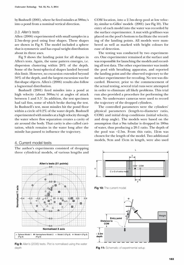
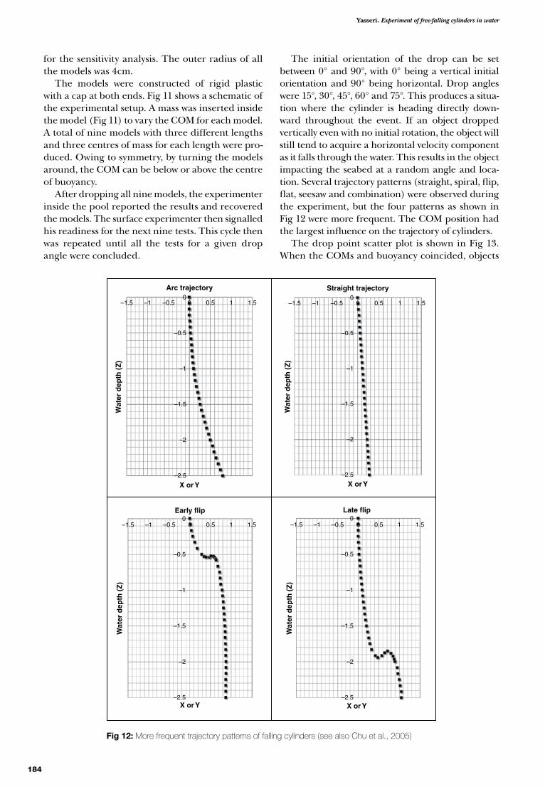
Yasseri Experiment of free-falling cylinders in water
184
for the sensitivity analysis The outer radius of all the models was 4cm
The models were constructed of rigid plastic with a cap at both ends Fig 11 shows a schematic of the experimental setup A mass was inserted inside the model (Fig 11) to vary the COM for each model A total of nine models with three different lengths and three centres of mass for each length were pro-duced Owing to symmetry by turning the models around the COM can be below or above the centre of buoyancy
After dropping all nine models the experimenter inside the pool reported the results and recovered the models The surface experimenter then signalled his readiness for the next nine tests This cycle then was repeated until all the tests for a given drop angle were concluded
The initial orientation of the drop can be set between 0deg and 90deg with 0deg being a vertical initial orientation and 90deg being horizontal Drop angles were 15deg 30deg 45deg 60deg and 75deg This produces a situa-tion where the cylinder is heading directly down-ward throughout the event If an object dropped vertically even with no initial rotation the object will still tend to acquire a horizontal velocity component as it falls through the water This results in the object impacting the seabed at a random angle and loca-tion Several trajectory patterns (straight spiral flip flat seesaw and combination) were observed during the experiment but the four patterns as shown in Fig 12 were more frequent The COM position had the largest influence on the trajectory of cylinders
The drop point scatter plot is shown in Fig 13 When the COMs and buoyancy coincided objects
Fig 12 More frequent trajectory patterns of falling cylinders (see also Chu et al 2005)
Arc trajectory Straight trajectory
Early flip Late flip
X or Y
Wat
er d
epth
(Z
)
ndash15 ndash1 ndash05 00
ndash05
ndash1
ndash15
ndash2
ndash25
05 1 15
X or Y
Wat
er d
epth
(Z
)
ndash15 ndash1 ndash05 00
ndash05
ndash1
ndash15
ndash2
ndash25
05 1 15
X or Y
Wat
er d
epth
(Z
)
ndash15 ndash1 ndash05 00
ndash05
ndash1
ndash15
ndash2
ndash25
05 1 15
X or Y
Wat
er d
epth
(Z
)
ndash15 ndash1 ndash05 00
ndash05
ndash1
ndash15
ndash2
ndash25
05 1 15
185
Underwater Technology Vol 32 No 3 2014
fell near the drop point for more than 90 of the time while a small distance between COM and the centre of volume (COV) caused the variability When the centre of buoyancy is ahead of the COM
the model flips while descending and experi-enced the largest excursion from the drop point When the drop angle is close to 90o and the centre of buoyancy and COM coincide then the descent is mostly vertical with only a slight slant When the buoyancy centre is above the mass centre models approach the floor at acute angles between 120deg and 180deg The trajectory patterns of each model type are affected by the size and shape of the mod-els The four generalised patterns were not shared among the various shapes but rather they were quite consistent within each shape type
Fig 14 shows the distance between the landing point and drop point in a lognormal probability plot It can be seen that the lognormal distribu-tion describes the probability of the landing spot fairly well Fig 15 shows results from another set of experiments where a cylinder with a length of 10cm and diameter of 12cm and a cube of 15cm times 15cm times 15cm were dropped using the same experimental setup These 140 points also follow a lognormal distbution similar to Fig 14 Fig 16 shows a few of the observed trajectories of the falling cylinder and cube in the second set of experiments
Fig 14 Authorrsquos results on a lognormal probability plot (324 points)
Probability plot of landing points for the current tests (324 points)
Standard normal variable
Dis
tan
ce b
etw
een
lan
din
g p
oin
t an
d t
he
dro
p p
oin
t
ndash3 ndash25 ndash2 ndash15 ndash1 ndash05 0 0505
005y = 01033exp(08147r)
R2 = 09828
Experimental dataExpon (Experimental data)
1 15 2 25 3
Fig 13 A plot of the landing point of all authorrsquos 324 tests
Landing points of 324 model cylinders droppedinto 25m of water
No
rmal
ised
Y a
xis
Normalised X axis
04
03
02
01
01 02 03 040
0
ndash01
ndash02
ndash03
ndash04
ndash04 ndash03 ndash02 ndash01
Yasseri Experiment of free-falling cylinders in water
186
5 Computational approachThe motion of three-dimensional rigid bodies freely falling through water has been addressed by many researchers Appendix A outlines the formu-lation necessary to track such motion MATLAB commercial software was used to solve these equa-tions Owing to a rigid body assumption tracking of one point gives enough data to plot the position of the falling object (Fig 17) Fig 18 shows some examples of trajectories using different values of control variables
These equations replicate the experimental results fairly well The method is applied to cylin-drical bodies initially released below the free sur-face in calm water Depending on the initial body orientation body aspect ratio and mass distribu-tion it is possible to identify key characteristic pat-terns of the body motion which compare remarkably with observations in the tank-drop tests The present study has a significant implica-tion to the manoeuvring of underwater vehicles Abelev et al (2007) presented experimental results of falling heavy cylindrical shapes which are in line with the authorrsquos results
6 Concluding remarksNot all falling objects travel straight downward under the influence of gravity even in the air Sometimes the falling objects follow complicated downward trajectories as they fall It is therefore
clear that any satisfactory explanation of this com-plex phenomenon must include a description of the instantaneous fluid forces experienced by the falling object as well as the inertial and gravita-tional effects that are present
Fig 16 A few of the observed trajectories for the second set of tests
Fig 17 Tracking the orientation of a falling object with position of COM lower than COV
Trajectory of a cylindrical object with heavy nose
10
0
ndash10
ndash20
ndash30
Wat
er d
epth
(m
)
Horizontal position (m)
ndash40
ndash50
ndash60
ndash70
ndash80ndash10 0 10 20 30 40 50 60 70 80
Nose position
Fig 15 Scatter plot for two shapes a short cylinder with lengthdiameter lt 1 and a small cube (140 points)
Landing points for dropped short cylinder anda cube of 150cm times 150cm times 150cm
04
03
02
01
ndash01
ndash02
ndash03
ndash04
ndash04 ndash03 ndash02 ndash01 0 01 02 03 04
Normalised X axis
No
rmal
ised
Y a
xis
0
Cylinder Drop point Box-shape
187
Underwater Technology Vol 32 No 3 2014
The entry of a solid into water or other liquids gives rise to a sequence of complex events The evolution of the air cavity behind the falling body after the initial impact significantly influences the dynamics and trajectory of low-speed projectiles (see eg Chu and Fan 2006 Chu and Ray 2006) The effect of air cavity dynamics is more pro-nounced in large body water entry Leaves tree seeds and paper cards falling in air are spectacular examples of time-dependent fluid dynamics at intermediate Reynolds numbers at which both inertial and viscous effects are important The tra-jectory of a falling card typically appears to be very complex with the card either oscillating from side to side (fluttering) or rotating and drifting side-ways (tumbling)
It is acknowledged that there are deficiencies in representing the landing point using a statistical distribution Fitting a distribution to a set of data only tells us how the dispersion would look The data behind the DNV recommendation (2010)
could not be located which makes the compari-sons between the DNV recommendation and the current experiment difficult In addition the log-normal curve may not represent the effect of all input parameters adequately It was chosen as the first approximation with an overall goal of developing a stochastic model evaluation Other distributions may be examined and could poten-tially represent the experimentally measured data better
Real objects of any significance are generally longer than 6m but still much smaller than the water depth for deepwater locations Thus the ratio of water depth to the object length is quite high Hence replicating it in a model test requires a very small model if the pool is not very deep It is desir-able that the choice of scale is representative of the offshore industryrsquos ratio of water depth to object length but at the same time it should be large enough to cover typical offshore tubular sizes The ratio of water depth to the tubular length for a
Fig 18 A few calculated trajectories for a falling cylinder with different orientation initial velocity and hydrodynamic conditions
Yasseri Experiment of free-falling cylinders in water
188
dropped tubular model of 12m in length in a water depth of 240m is 20 Therefore for a pool depth of 25m the model length should be around 120mm
Ingram (1991) surmises there is a depth beyond which an object would fall flat implying there is a single pattern in deep water However no single pattern was observed in these tests
Pulling together all tests reported here the fol-lowing observations can be made about the land-ing location of free-falling cylinders
bullAbout 50 of the time objects land within 10 of the water depth
bullAbout 80 of the time objects land within 20 of the water depth
bullAbout 90 of the time objects land within 30 of water depth
bullAbout 95 of the time objects land within 40 of water depth
bullAbout 98 of the time objects land within 50 of water depth
These tests were performed in pools where the water surface only experiences small ripples However there is significantly more undulation in the ocean surface Such undulation will cause more deviation to the object and help it to travel further (Fig 19)
ReferencesAanesland V (1987) Numerical and experimental investi-
gation of accidentally falling drilling pipes OTC 5494 19th Offshore Technology Conference April 1987 Houston USA
Abelev AV Valent PJ and Holland KT (2007) Behaviour of a large cylinder in free fall through water IEEE Journal of Ocean Engineering 32 10ndash20
Allen CR (2006) Mine drop experiment II with operational mines shapes (MIDEX II) MS Thesis Naval Postgraduate School Monterey CA USA 306pp Available at httpfacultynpsedupcchuweb_paperthesis06Mar_Allenpdf last accessed lt14 September 2014gt
Bushnell JM (2001) Tail separation and density effects on the underwater trajectory of the JDAM MS Thesis Naval Postgraduate School Monterey CA USA 88pp Available at httpcalhounnpsedupublichandle109454406 last accessed lt14 September 2014gt
Chu PC (2009) Mine impact burial prediction from one to three dimensions ASME Journal of Applied Mechanics Review 62
Chu PC and Fan CW (2006) Prediction of falling cylinder through air-water-sediment columns ASME Journal of Applied Mechanics Review 73 300ndash314
Chu PC and Ray G (2006) Prediction of high speed rigid body manoeuvring in air-water-sediment columns In Rahman M and Brebbia CA (eds) Advances in Fluid Mechanics V Southampton UK WIT Press 123ndash132
Chu PC Fan CW Evans AD and Gilles AF (2004) Triple coordinate transforms for prediction of falling cylinder through the water column Journal of Applied Mechanics 71 292ndash298
Chu PC Gilles AF and Fan CW (2005) Experiment of falling cylinder through the water column Experimental Thermal and Fluid Science 29 555ndash568
Colwill RD and Ahilan RV (1992) Reliability analysis of the behaviour of dropped objects OTC 6918 24th Offshore Technology Conference April 1992 Houston USA
Det Norske Veritas (DNV) (2010) Risk assessment of pipeline protection Recommended practice No DNV-RP- F107 Olso Norway DNV 45pp
Evans A (2002) Hydrodynamics of mine impact burial MS Thesis Naval Postgraduate School Monterey CA 2002 Available at httpcalhounnpseduhandle10945 5310show=full last accessed lt14 September 2014gt
Friedman A Zilman G and Miloh T (2003) Dynamics of a body falling in waves In Proceedings of 18th Interna-tional Workshop of Water Waves and Floating Bodies (IWWWFB) Ann Arbour MI USA
Gilles A (2001) Mine Drop Experiment (MIDEX) MS The-sis Naval Postgraduate School Monterey CA USA 446pp Available at httpfacultynpsedupcchuweb_paperthesisgillespdf last accessed lt14 September 2014gt
Ingram JG (1991) Experimental modelling and risk assess-ment of dropped offshore tubulars MS Thesis School of Industrial and Manufacturing Science Cranfield Insti-tute of Technology Cranfield UK
Kim Y Lin KY and Yue KD (2002) Motion dynamics of three-dimensional bodies falling through water In Rainey RCT and Lee SF (eds) Proceedings of 17th International Workshop of Water Waves and Floating Bodies (IWWWFB) London WS Atkins Consultants 81ndash84 Available at httpwwwiwwwfborgAbstractsiwwwfb17iwwwfb17_21pdf last accessed lt14 September 2014gt
Ray G (2006) Bomb strike experiments for mine counter-measure MS Thesis Naval Postgraduate School Monte-rey CA USA 197pp Available at httpfacultynpsedupcchuweb_paperthesis06Mar_Raypdf last accessed lt14 September 2014gt
Von Mises R (1959) Theory of Flight 1st edition New York Dover Publications Inc 629pp
Wierzbicki T and Yue DK (1986) Impact damage of Chal-lenger crew compartment Journal of Spacecraft and Rockets 23 646ndash654
Yasseri S (1997) Risk-based decision analysis for the protec-tion of marine pipelines from dropped objects In Proceed-ings of 7th International Offshore and Polar Engineering Conference Honolulu USA 251ndash256
Fig 19 The effect of undulating sea surface on the trajectory and drifting
Drift owing to object hitting the wave atdifferent location
Wave slope
Entry angle
189
Underwater Technology Vol 32 No 3 2014
Appendix A
Rigid body dynamics of a cylinder falling through waterThere are various methods of describing the motion of a rigid body see for example Von Mises (1959) Chu et al (2005) Wierzbicki and Yue (1986) Kim et al (2002) and Friedman et al (2003) In the fol-lowing equations which are needed to track the dynamics of motion of three-dimensional rigid bod-ies falling through water (Chu et al 2005) are given
Fig 20 shows a right circular symmetric cylinder whose centres of mass (X) and volume (B) are on the cylinderrsquos longitudinal axis Parameters (L d x) denote the cylinderrsquos length diameter and the dis-tance between the two points (X B) The positive case is when the centre of mass (COM) is lower than the centre of volume (COV) ie x is positive (Evans 2002)
Three orthogonal right-handed coordinate sys-tems (Fig 21) are used describe the dynamics of a falling cylinder through the water which are E-coordinate M-coordinate and F-coordinate sys-tems The body and buoyancy forces and their moments are given in the E-coordinate system the hydrodynamic forces (drag lift and inertia forces) and their moments are given in the F-coordinate and the cylinderrsquos moments of gyration are given in the M-coordinate The E-coordinate system is fixed to the Earthrsquos surface with horizontal sides as x and y axes are parallel with the Earthrsquos surface (along the two sides of the pool) and vertical direc-tion as z axis (upward positive Fig 20)
Suppose the cylinder is falling into the water The cylinder rotates around its main axis (r1) with an angle ψ1 and an angular velocity of Ω Its position
is represented by the COM and its orientation is represented by two angles ψ2 and ψ3 (Fig 3) Here ψ2 is the angle between the r1 axis and the horizon-tal plane and ψ3 is the angle between the projec-tion of the main axis in the (x y) plane and the x axis The angle (ψ2 + π2) is usually called attitude
The relative coordinate is rigidly connected with the cylinder The origin (O) of the relative coordi-nate system coincides with the COM the r1 axis is along the central line of the cylinder the r2 axis is perpendicular to the plane constructed by r1 axis and z-axis (r1-z plane) and the r3-axis lies in the (r1-z) plane and is perpendicular to r1 axis The axes (x y z) and (r1 r2 r3) follows the right-hand rule
Let V = (V1 V2 V3 ) the three components of the velocity of COM ie the origin velocity of the coor-dinate system (r1 r2 r3) The geometric centre (GC) is located at (x 0 0) if for GC below COM x gt 0 and for GC above COM x lt 0 The relative coordinate system (r1 r2 r3) is obtained by one translation and two rotations ψ2 and ψ3 of the E-coordinate system Let the position vector (P) be represented by PE and
Fig 20 M-coordinate with the COM as the origin X (im jm) x is the distance between the COV (B) and COM (X) L and d are the cylinderrsquos length and diameter (Chu et al 2005)
2
d
L2L
B
xjm
imX
z (k )
y ( j )
kmjmψ2
imo ψ3
x (i )
obull
kf
jf
ifobull
V1
V2 Vr
Fig 21 Cylinder orientation and relative coordinate system
Yasseri Experiment of free-falling cylinders in water
190
PB in the Earth and relative coordinate systems PE and PB are connected by
PE =minus
minus
cos sin
sin cos
cos sin
si
ψ ψψ ψ
ψ ψ
3 3
3 3
2 2
0
0
0 0 1
0
0 1 0
nn cosψ ψ2 20
+
lowast
lowast
lowast
P
x
y
zB
m
m
m
(A1)
where (xm ym zm) represent the position of COM in the Earthrsquos coordinate system
The motion of a solid object falling through a fluid is governed by two principles (1) momentum balance and (2) moment of momentum balance Let Vw = (Vw1 Vw2 Vw3) be the water velocity and (ω1 ω2 ω3) be the components of the angular velocity referring to the direction of the relative coordinate system Variables are made non-dimensional by
tgL
tLg
VV
gL= = =lowast lowast
lowast
ω (A2)
where g is the gravitational acceleration and L the length of the cylinder The non-dimensional momentum equations for COM are given by (Van Mises 1959)
dVdt
V VFg
w12 3 3 2 2
1+ minus =minus
+forall
lowast
ω ωρ ρ
ρψ
ρsin (A3)
dVdt
VFg
23 1
2+ =forall
lowast
ωρ
(A4)
dVdt
VFg
w32 1 2
3minus =minus
+forall
lowast
ωρ ρ
ρψ
ρcos (A5)
where forall is the volume of the cylinder ρ is the cylinder density ρw is the water density and (F1
F2 F3
) are the components of fluid drag The non-dimensional equations of the moment of momentum for circu-lar symmetric cylinder are
ddt
J JJ
LMg J
Ω+
minus=
lowast3 2
12 3
1
1
ω ω (A6)
ddt
x LJ
LMg J
wω ρ ρψ2
22
2
2
= minusforall minus
+lowast lowast( )
cos (A7)
ddt
LMg J
ω3 3
3
=lowast
(A8)
where x is the distance between COM and GC and (M1
M2 M3
) are the components of the moment
owing to drag (J1 J2 J3) The three moments of gyration are
J r r dm J r r dm
J r r dm
1 22
32
2 32
12
3 12
22
= + = +
= +
int intint
lowast lowast
lowast
( ) ( )
( )and (A9)
The orientation of the cylinder (ψ2 ψ3) is deter-mined by
ddt
ddt
ψω ψ
ψω2
2 23
3= = cos (A10)
The eight non-dimensional nonlinear equations (A2 to A5) (A6 to A8) and (A10) are the funda-mental equations for determining the cylinder movement in the water
All the equations were solved using the 4th order Runge-Kutta scheme for integration with time in MATLAB At any instant the hydrody-namic loads were computed using a panel method
Appendix B
Probability plottingA method that may be used to visualise distri-butions and estimate parameters is probability plotting also referred to as linear least-squares regression or regression on ordered statistics This technique involves finding a probability and data scale that plots the cumulative distribution func-tion (CDF) of a hypothesised distribution as a straight line The corresponding linearity of the CDF for the sample data provides a measure of the goodness-of-fit of the hypothesised distribution
The n test results (ri r2hellip rn) were arranged in increasing order the mth value is marked on the verti-cal axis and corresponds to a cumulative probability of p = m(N + 1) marked on the horizontal axis Then the value of standardised normal variable for each p was calculated using the normal distribution table
The distance between the drop point and the landing point were ordered in terms of increasing magnitude in a table and the cumulative frequency of each ratio were determined which is equal to the cumulative probability of p For each p the value for the corresponding standard normally distributed variable is then calculated and noted in that table Samples of (Zi ri) are plotted on the logarithmic normal distribution graph as shown in Fig 14
The straight line equation that best fits the sam-ples can be written as
y = a e bx (B1)
where a and b are constants
191
Underwater Technology Vol 32 No 3 2014
Taking logarithm of both sides of this equation results in
lny = lnα + bx (B2)
The standard normal variable becomes
sr
rii s= = +minusln λ
ζλ ζ or ln (B3)
Equating two equations gives the ordinate inter-cept of the straight line and its slope ie
λ = lnα amp b = ζ (B4)
Then the mean value of landing points (r) is
r = rE = exp(λ + 05ζ2) (B5)
From Fig 14 it can be seen that they can be approximated by the following straight line
y = 01033e08147x (B6)
λ = ln(01033) = minus227012 ζ = b = 08147 (B7)
r = rE = exp(minus227012 + 05 times 081472)= 01439 (1439 of the water depth) (B8)
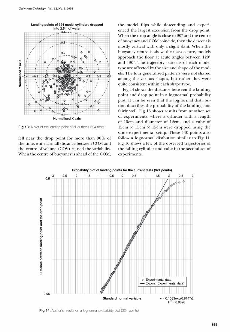
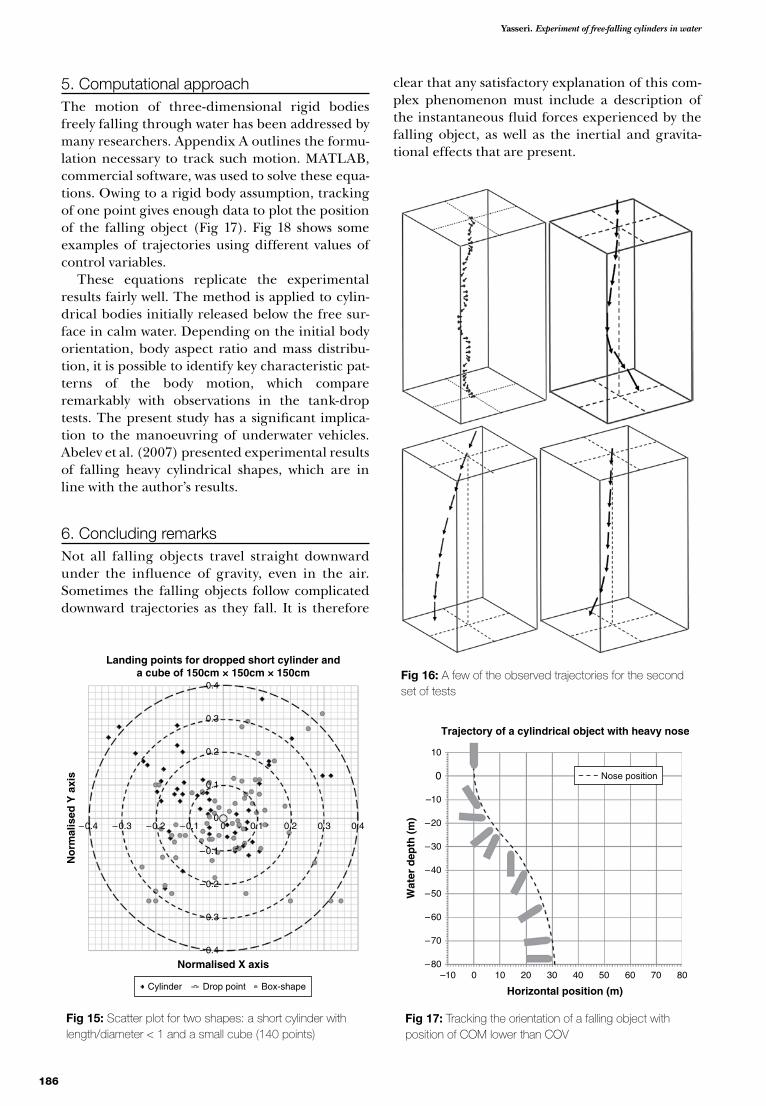
Yasseri Experiment of free-falling cylinders in water
186
5 Computational approachThe motion of three-dimensional rigid bodies freely falling through water has been addressed by many researchers Appendix A outlines the formu-lation necessary to track such motion MATLAB commercial software was used to solve these equa-tions Owing to a rigid body assumption tracking of one point gives enough data to plot the position of the falling object (Fig 17) Fig 18 shows some examples of trajectories using different values of control variables
These equations replicate the experimental results fairly well The method is applied to cylin-drical bodies initially released below the free sur-face in calm water Depending on the initial body orientation body aspect ratio and mass distribu-tion it is possible to identify key characteristic pat-terns of the body motion which compare remarkably with observations in the tank-drop tests The present study has a significant implica-tion to the manoeuvring of underwater vehicles Abelev et al (2007) presented experimental results of falling heavy cylindrical shapes which are in line with the authorrsquos results
6 Concluding remarksNot all falling objects travel straight downward under the influence of gravity even in the air Sometimes the falling objects follow complicated downward trajectories as they fall It is therefore
clear that any satisfactory explanation of this com-plex phenomenon must include a description of the instantaneous fluid forces experienced by the falling object as well as the inertial and gravita-tional effects that are present
Fig 16 A few of the observed trajectories for the second set of tests
Fig 17 Tracking the orientation of a falling object with position of COM lower than COV
Trajectory of a cylindrical object with heavy nose
10
0
ndash10
ndash20
ndash30
Wat
er d
epth
(m
)
Horizontal position (m)
ndash40
ndash50
ndash60
ndash70
ndash80ndash10 0 10 20 30 40 50 60 70 80
Nose position
Fig 15 Scatter plot for two shapes a short cylinder with lengthdiameter lt 1 and a small cube (140 points)
Landing points for dropped short cylinder anda cube of 150cm times 150cm times 150cm
04
03
02
01
ndash01
ndash02
ndash03
ndash04
ndash04 ndash03 ndash02 ndash01 0 01 02 03 04
Normalised X axis
No
rmal
ised
Y a
xis
0
Cylinder Drop point Box-shape
187
Underwater Technology Vol 32 No 3 2014
The entry of a solid into water or other liquids gives rise to a sequence of complex events The evolution of the air cavity behind the falling body after the initial impact significantly influences the dynamics and trajectory of low-speed projectiles (see eg Chu and Fan 2006 Chu and Ray 2006) The effect of air cavity dynamics is more pro-nounced in large body water entry Leaves tree seeds and paper cards falling in air are spectacular examples of time-dependent fluid dynamics at intermediate Reynolds numbers at which both inertial and viscous effects are important The tra-jectory of a falling card typically appears to be very complex with the card either oscillating from side to side (fluttering) or rotating and drifting side-ways (tumbling)
It is acknowledged that there are deficiencies in representing the landing point using a statistical distribution Fitting a distribution to a set of data only tells us how the dispersion would look The data behind the DNV recommendation (2010)
could not be located which makes the compari-sons between the DNV recommendation and the current experiment difficult In addition the log-normal curve may not represent the effect of all input parameters adequately It was chosen as the first approximation with an overall goal of developing a stochastic model evaluation Other distributions may be examined and could poten-tially represent the experimentally measured data better
Real objects of any significance are generally longer than 6m but still much smaller than the water depth for deepwater locations Thus the ratio of water depth to the object length is quite high Hence replicating it in a model test requires a very small model if the pool is not very deep It is desir-able that the choice of scale is representative of the offshore industryrsquos ratio of water depth to object length but at the same time it should be large enough to cover typical offshore tubular sizes The ratio of water depth to the tubular length for a
Fig 18 A few calculated trajectories for a falling cylinder with different orientation initial velocity and hydrodynamic conditions
Yasseri Experiment of free-falling cylinders in water
188
dropped tubular model of 12m in length in a water depth of 240m is 20 Therefore for a pool depth of 25m the model length should be around 120mm
Ingram (1991) surmises there is a depth beyond which an object would fall flat implying there is a single pattern in deep water However no single pattern was observed in these tests
Pulling together all tests reported here the fol-lowing observations can be made about the land-ing location of free-falling cylinders
bullAbout 50 of the time objects land within 10 of the water depth
bullAbout 80 of the time objects land within 20 of the water depth
bullAbout 90 of the time objects land within 30 of water depth
bullAbout 95 of the time objects land within 40 of water depth
bullAbout 98 of the time objects land within 50 of water depth
These tests were performed in pools where the water surface only experiences small ripples However there is significantly more undulation in the ocean surface Such undulation will cause more deviation to the object and help it to travel further (Fig 19)
ReferencesAanesland V (1987) Numerical and experimental investi-
gation of accidentally falling drilling pipes OTC 5494 19th Offshore Technology Conference April 1987 Houston USA
Abelev AV Valent PJ and Holland KT (2007) Behaviour of a large cylinder in free fall through water IEEE Journal of Ocean Engineering 32 10ndash20
Allen CR (2006) Mine drop experiment II with operational mines shapes (MIDEX II) MS Thesis Naval Postgraduate School Monterey CA USA 306pp Available at httpfacultynpsedupcchuweb_paperthesis06Mar_Allenpdf last accessed lt14 September 2014gt
Bushnell JM (2001) Tail separation and density effects on the underwater trajectory of the JDAM MS Thesis Naval Postgraduate School Monterey CA USA 88pp Available at httpcalhounnpsedupublichandle109454406 last accessed lt14 September 2014gt
Chu PC (2009) Mine impact burial prediction from one to three dimensions ASME Journal of Applied Mechanics Review 62
Chu PC and Fan CW (2006) Prediction of falling cylinder through air-water-sediment columns ASME Journal of Applied Mechanics Review 73 300ndash314
Chu PC and Ray G (2006) Prediction of high speed rigid body manoeuvring in air-water-sediment columns In Rahman M and Brebbia CA (eds) Advances in Fluid Mechanics V Southampton UK WIT Press 123ndash132
Chu PC Fan CW Evans AD and Gilles AF (2004) Triple coordinate transforms for prediction of falling cylinder through the water column Journal of Applied Mechanics 71 292ndash298
Chu PC Gilles AF and Fan CW (2005) Experiment of falling cylinder through the water column Experimental Thermal and Fluid Science 29 555ndash568
Colwill RD and Ahilan RV (1992) Reliability analysis of the behaviour of dropped objects OTC 6918 24th Offshore Technology Conference April 1992 Houston USA
Det Norske Veritas (DNV) (2010) Risk assessment of pipeline protection Recommended practice No DNV-RP- F107 Olso Norway DNV 45pp
Evans A (2002) Hydrodynamics of mine impact burial MS Thesis Naval Postgraduate School Monterey CA 2002 Available at httpcalhounnpseduhandle10945 5310show=full last accessed lt14 September 2014gt
Friedman A Zilman G and Miloh T (2003) Dynamics of a body falling in waves In Proceedings of 18th Interna-tional Workshop of Water Waves and Floating Bodies (IWWWFB) Ann Arbour MI USA
Gilles A (2001) Mine Drop Experiment (MIDEX) MS The-sis Naval Postgraduate School Monterey CA USA 446pp Available at httpfacultynpsedupcchuweb_paperthesisgillespdf last accessed lt14 September 2014gt
Ingram JG (1991) Experimental modelling and risk assess-ment of dropped offshore tubulars MS Thesis School of Industrial and Manufacturing Science Cranfield Insti-tute of Technology Cranfield UK
Kim Y Lin KY and Yue KD (2002) Motion dynamics of three-dimensional bodies falling through water In Rainey RCT and Lee SF (eds) Proceedings of 17th International Workshop of Water Waves and Floating Bodies (IWWWFB) London WS Atkins Consultants 81ndash84 Available at httpwwwiwwwfborgAbstractsiwwwfb17iwwwfb17_21pdf last accessed lt14 September 2014gt
Ray G (2006) Bomb strike experiments for mine counter-measure MS Thesis Naval Postgraduate School Monte-rey CA USA 197pp Available at httpfacultynpsedupcchuweb_paperthesis06Mar_Raypdf last accessed lt14 September 2014gt
Von Mises R (1959) Theory of Flight 1st edition New York Dover Publications Inc 629pp
Wierzbicki T and Yue DK (1986) Impact damage of Chal-lenger crew compartment Journal of Spacecraft and Rockets 23 646ndash654
Yasseri S (1997) Risk-based decision analysis for the protec-tion of marine pipelines from dropped objects In Proceed-ings of 7th International Offshore and Polar Engineering Conference Honolulu USA 251ndash256
Fig 19 The effect of undulating sea surface on the trajectory and drifting
Drift owing to object hitting the wave atdifferent location
Wave slope
Entry angle
189
Underwater Technology Vol 32 No 3 2014
Appendix A
Rigid body dynamics of a cylinder falling through waterThere are various methods of describing the motion of a rigid body see for example Von Mises (1959) Chu et al (2005) Wierzbicki and Yue (1986) Kim et al (2002) and Friedman et al (2003) In the fol-lowing equations which are needed to track the dynamics of motion of three-dimensional rigid bod-ies falling through water (Chu et al 2005) are given
Fig 20 shows a right circular symmetric cylinder whose centres of mass (X) and volume (B) are on the cylinderrsquos longitudinal axis Parameters (L d x) denote the cylinderrsquos length diameter and the dis-tance between the two points (X B) The positive case is when the centre of mass (COM) is lower than the centre of volume (COV) ie x is positive (Evans 2002)
Three orthogonal right-handed coordinate sys-tems (Fig 21) are used describe the dynamics of a falling cylinder through the water which are E-coordinate M-coordinate and F-coordinate sys-tems The body and buoyancy forces and their moments are given in the E-coordinate system the hydrodynamic forces (drag lift and inertia forces) and their moments are given in the F-coordinate and the cylinderrsquos moments of gyration are given in the M-coordinate The E-coordinate system is fixed to the Earthrsquos surface with horizontal sides as x and y axes are parallel with the Earthrsquos surface (along the two sides of the pool) and vertical direc-tion as z axis (upward positive Fig 20)
Suppose the cylinder is falling into the water The cylinder rotates around its main axis (r1) with an angle ψ1 and an angular velocity of Ω Its position
is represented by the COM and its orientation is represented by two angles ψ2 and ψ3 (Fig 3) Here ψ2 is the angle between the r1 axis and the horizon-tal plane and ψ3 is the angle between the projec-tion of the main axis in the (x y) plane and the x axis The angle (ψ2 + π2) is usually called attitude
The relative coordinate is rigidly connected with the cylinder The origin (O) of the relative coordi-nate system coincides with the COM the r1 axis is along the central line of the cylinder the r2 axis is perpendicular to the plane constructed by r1 axis and z-axis (r1-z plane) and the r3-axis lies in the (r1-z) plane and is perpendicular to r1 axis The axes (x y z) and (r1 r2 r3) follows the right-hand rule
Let V = (V1 V2 V3 ) the three components of the velocity of COM ie the origin velocity of the coor-dinate system (r1 r2 r3) The geometric centre (GC) is located at (x 0 0) if for GC below COM x gt 0 and for GC above COM x lt 0 The relative coordinate system (r1 r2 r3) is obtained by one translation and two rotations ψ2 and ψ3 of the E-coordinate system Let the position vector (P) be represented by PE and
Fig 20 M-coordinate with the COM as the origin X (im jm) x is the distance between the COV (B) and COM (X) L and d are the cylinderrsquos length and diameter (Chu et al 2005)
2
d
L2L
B
xjm
imX
z (k )
y ( j )
kmjmψ2
imo ψ3
x (i )
obull
kf
jf
ifobull
V1
V2 Vr
Fig 21 Cylinder orientation and relative coordinate system
Yasseri Experiment of free-falling cylinders in water
190
PB in the Earth and relative coordinate systems PE and PB are connected by
PE =minus
minus
cos sin
sin cos
cos sin
si
ψ ψψ ψ
ψ ψ
3 3
3 3
2 2
0
0
0 0 1
0
0 1 0
nn cosψ ψ2 20
+
lowast
lowast
lowast
P
x
y
zB
m
m
m
(A1)
where (xm ym zm) represent the position of COM in the Earthrsquos coordinate system
The motion of a solid object falling through a fluid is governed by two principles (1) momentum balance and (2) moment of momentum balance Let Vw = (Vw1 Vw2 Vw3) be the water velocity and (ω1 ω2 ω3) be the components of the angular velocity referring to the direction of the relative coordinate system Variables are made non-dimensional by
tgL
tLg
VV
gL= = =lowast lowast
lowast
ω (A2)
where g is the gravitational acceleration and L the length of the cylinder The non-dimensional momentum equations for COM are given by (Van Mises 1959)
dVdt
V VFg
w12 3 3 2 2
1+ minus =minus
+forall
lowast
ω ωρ ρ
ρψ
ρsin (A3)
dVdt
VFg
23 1
2+ =forall
lowast
ωρ
(A4)
dVdt
VFg
w32 1 2
3minus =minus
+forall
lowast
ωρ ρ
ρψ
ρcos (A5)
where forall is the volume of the cylinder ρ is the cylinder density ρw is the water density and (F1
F2 F3
) are the components of fluid drag The non-dimensional equations of the moment of momentum for circu-lar symmetric cylinder are
ddt
J JJ
LMg J
Ω+
minus=
lowast3 2
12 3
1
1
ω ω (A6)
ddt
x LJ
LMg J
wω ρ ρψ2
22
2
2
= minusforall minus
+lowast lowast( )
cos (A7)
ddt
LMg J
ω3 3
3
=lowast
(A8)
where x is the distance between COM and GC and (M1
M2 M3
) are the components of the moment
owing to drag (J1 J2 J3) The three moments of gyration are
J r r dm J r r dm
J r r dm
1 22
32
2 32
12
3 12
22
= + = +
= +
int intint
lowast lowast
lowast
( ) ( )
( )and (A9)
The orientation of the cylinder (ψ2 ψ3) is deter-mined by
ddt
ddt
ψω ψ
ψω2
2 23
3= = cos (A10)
The eight non-dimensional nonlinear equations (A2 to A5) (A6 to A8) and (A10) are the funda-mental equations for determining the cylinder movement in the water
All the equations were solved using the 4th order Runge-Kutta scheme for integration with time in MATLAB At any instant the hydrody-namic loads were computed using a panel method
Appendix B
Probability plottingA method that may be used to visualise distri-butions and estimate parameters is probability plotting also referred to as linear least-squares regression or regression on ordered statistics This technique involves finding a probability and data scale that plots the cumulative distribution func-tion (CDF) of a hypothesised distribution as a straight line The corresponding linearity of the CDF for the sample data provides a measure of the goodness-of-fit of the hypothesised distribution
The n test results (ri r2hellip rn) were arranged in increasing order the mth value is marked on the verti-cal axis and corresponds to a cumulative probability of p = m(N + 1) marked on the horizontal axis Then the value of standardised normal variable for each p was calculated using the normal distribution table
The distance between the drop point and the landing point were ordered in terms of increasing magnitude in a table and the cumulative frequency of each ratio were determined which is equal to the cumulative probability of p For each p the value for the corresponding standard normally distributed variable is then calculated and noted in that table Samples of (Zi ri) are plotted on the logarithmic normal distribution graph as shown in Fig 14
The straight line equation that best fits the sam-ples can be written as
y = a e bx (B1)
where a and b are constants
191
Underwater Technology Vol 32 No 3 2014
Taking logarithm of both sides of this equation results in
lny = lnα + bx (B2)
The standard normal variable becomes
sr
rii s= = +minusln λ
ζλ ζ or ln (B3)
Equating two equations gives the ordinate inter-cept of the straight line and its slope ie
λ = lnα amp b = ζ (B4)
Then the mean value of landing points (r) is
r = rE = exp(λ + 05ζ2) (B5)
From Fig 14 it can be seen that they can be approximated by the following straight line
y = 01033e08147x (B6)
λ = ln(01033) = minus227012 ζ = b = 08147 (B7)
r = rE = exp(minus227012 + 05 times 081472)= 01439 (1439 of the water depth) (B8)
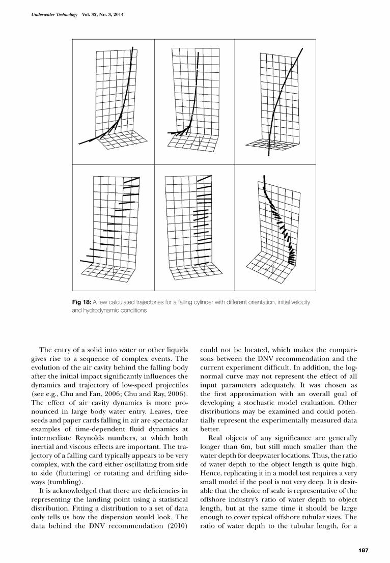
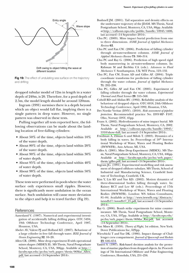
Yasseri Experiment of free-falling cylinders in water
188
dropped tubular model of 12m in length in a water depth of 240m is 20 Therefore for a pool depth of 25m the model length should be around 120mm
Ingram (1991) surmises there is a depth beyond which an object would fall flat implying there is a single pattern in deep water However no single pattern was observed in these tests
Pulling together all tests reported here the fol-lowing observations can be made about the land-ing location of free-falling cylinders
bullAbout 50 of the time objects land within 10 of the water depth
bullAbout 80 of the time objects land within 20 of the water depth
bullAbout 90 of the time objects land within 30 of water depth
bullAbout 95 of the time objects land within 40 of water depth
bullAbout 98 of the time objects land within 50 of water depth
These tests were performed in pools where the water surface only experiences small ripples However there is significantly more undulation in the ocean surface Such undulation will cause more deviation to the object and help it to travel further (Fig 19)
ReferencesAanesland V (1987) Numerical and experimental investi-
gation of accidentally falling drilling pipes OTC 5494 19th Offshore Technology Conference April 1987 Houston USA
Abelev AV Valent PJ and Holland KT (2007) Behaviour of a large cylinder in free fall through water IEEE Journal of Ocean Engineering 32 10ndash20
Allen CR (2006) Mine drop experiment II with operational mines shapes (MIDEX II) MS Thesis Naval Postgraduate School Monterey CA USA 306pp Available at httpfacultynpsedupcchuweb_paperthesis06Mar_Allenpdf last accessed lt14 September 2014gt
Bushnell JM (2001) Tail separation and density effects on the underwater trajectory of the JDAM MS Thesis Naval Postgraduate School Monterey CA USA 88pp Available at httpcalhounnpsedupublichandle109454406 last accessed lt14 September 2014gt
Chu PC (2009) Mine impact burial prediction from one to three dimensions ASME Journal of Applied Mechanics Review 62
Chu PC and Fan CW (2006) Prediction of falling cylinder through air-water-sediment columns ASME Journal of Applied Mechanics Review 73 300ndash314
Chu PC and Ray G (2006) Prediction of high speed rigid body manoeuvring in air-water-sediment columns In Rahman M and Brebbia CA (eds) Advances in Fluid Mechanics V Southampton UK WIT Press 123ndash132
Chu PC Fan CW Evans AD and Gilles AF (2004) Triple coordinate transforms for prediction of falling cylinder through the water column Journal of Applied Mechanics 71 292ndash298
Chu PC Gilles AF and Fan CW (2005) Experiment of falling cylinder through the water column Experimental Thermal and Fluid Science 29 555ndash568
Colwill RD and Ahilan RV (1992) Reliability analysis of the behaviour of dropped objects OTC 6918 24th Offshore Technology Conference April 1992 Houston USA
Det Norske Veritas (DNV) (2010) Risk assessment of pipeline protection Recommended practice No DNV-RP- F107 Olso Norway DNV 45pp
Evans A (2002) Hydrodynamics of mine impact burial MS Thesis Naval Postgraduate School Monterey CA 2002 Available at httpcalhounnpseduhandle10945 5310show=full last accessed lt14 September 2014gt
Friedman A Zilman G and Miloh T (2003) Dynamics of a body falling in waves In Proceedings of 18th Interna-tional Workshop of Water Waves and Floating Bodies (IWWWFB) Ann Arbour MI USA
Gilles A (2001) Mine Drop Experiment (MIDEX) MS The-sis Naval Postgraduate School Monterey CA USA 446pp Available at httpfacultynpsedupcchuweb_paperthesisgillespdf last accessed lt14 September 2014gt
Ingram JG (1991) Experimental modelling and risk assess-ment of dropped offshore tubulars MS Thesis School of Industrial and Manufacturing Science Cranfield Insti-tute of Technology Cranfield UK
Kim Y Lin KY and Yue KD (2002) Motion dynamics of three-dimensional bodies falling through water In Rainey RCT and Lee SF (eds) Proceedings of 17th International Workshop of Water Waves and Floating Bodies (IWWWFB) London WS Atkins Consultants 81ndash84 Available at httpwwwiwwwfborgAbstractsiwwwfb17iwwwfb17_21pdf last accessed lt14 September 2014gt
Ray G (2006) Bomb strike experiments for mine counter-measure MS Thesis Naval Postgraduate School Monte-rey CA USA 197pp Available at httpfacultynpsedupcchuweb_paperthesis06Mar_Raypdf last accessed lt14 September 2014gt
Von Mises R (1959) Theory of Flight 1st edition New York Dover Publications Inc 629pp
Wierzbicki T and Yue DK (1986) Impact damage of Chal-lenger crew compartment Journal of Spacecraft and Rockets 23 646ndash654
Yasseri S (1997) Risk-based decision analysis for the protec-tion of marine pipelines from dropped objects In Proceed-ings of 7th International Offshore and Polar Engineering Conference Honolulu USA 251ndash256
Fig 19 The effect of undulating sea surface on the trajectory and drifting
Drift owing to object hitting the wave atdifferent location
Wave slope
Entry angle
189
Underwater Technology Vol 32 No 3 2014
Appendix A
Rigid body dynamics of a cylinder falling through waterThere are various methods of describing the motion of a rigid body see for example Von Mises (1959) Chu et al (2005) Wierzbicki and Yue (1986) Kim et al (2002) and Friedman et al (2003) In the fol-lowing equations which are needed to track the dynamics of motion of three-dimensional rigid bod-ies falling through water (Chu et al 2005) are given
Fig 20 shows a right circular symmetric cylinder whose centres of mass (X) and volume (B) are on the cylinderrsquos longitudinal axis Parameters (L d x) denote the cylinderrsquos length diameter and the dis-tance between the two points (X B) The positive case is when the centre of mass (COM) is lower than the centre of volume (COV) ie x is positive (Evans 2002)
Three orthogonal right-handed coordinate sys-tems (Fig 21) are used describe the dynamics of a falling cylinder through the water which are E-coordinate M-coordinate and F-coordinate sys-tems The body and buoyancy forces and their moments are given in the E-coordinate system the hydrodynamic forces (drag lift and inertia forces) and their moments are given in the F-coordinate and the cylinderrsquos moments of gyration are given in the M-coordinate The E-coordinate system is fixed to the Earthrsquos surface with horizontal sides as x and y axes are parallel with the Earthrsquos surface (along the two sides of the pool) and vertical direc-tion as z axis (upward positive Fig 20)
Suppose the cylinder is falling into the water The cylinder rotates around its main axis (r1) with an angle ψ1 and an angular velocity of Ω Its position
is represented by the COM and its orientation is represented by two angles ψ2 and ψ3 (Fig 3) Here ψ2 is the angle between the r1 axis and the horizon-tal plane and ψ3 is the angle between the projec-tion of the main axis in the (x y) plane and the x axis The angle (ψ2 + π2) is usually called attitude
The relative coordinate is rigidly connected with the cylinder The origin (O) of the relative coordi-nate system coincides with the COM the r1 axis is along the central line of the cylinder the r2 axis is perpendicular to the plane constructed by r1 axis and z-axis (r1-z plane) and the r3-axis lies in the (r1-z) plane and is perpendicular to r1 axis The axes (x y z) and (r1 r2 r3) follows the right-hand rule
Let V = (V1 V2 V3 ) the three components of the velocity of COM ie the origin velocity of the coor-dinate system (r1 r2 r3) The geometric centre (GC) is located at (x 0 0) if for GC below COM x gt 0 and for GC above COM x lt 0 The relative coordinate system (r1 r2 r3) is obtained by one translation and two rotations ψ2 and ψ3 of the E-coordinate system Let the position vector (P) be represented by PE and
Fig 20 M-coordinate with the COM as the origin X (im jm) x is the distance between the COV (B) and COM (X) L and d are the cylinderrsquos length and diameter (Chu et al 2005)
2
d
L2L
B
xjm
imX
z (k )
y ( j )
kmjmψ2
imo ψ3
x (i )
obull
kf
jf
ifobull
V1
V2 Vr
Fig 21 Cylinder orientation and relative coordinate system
Yasseri Experiment of free-falling cylinders in water
190
PB in the Earth and relative coordinate systems PE and PB are connected by
PE =minus
minus
cos sin
sin cos
cos sin
si
ψ ψψ ψ
ψ ψ
3 3
3 3
2 2
0
0
0 0 1
0
0 1 0
nn cosψ ψ2 20
+
lowast
lowast
lowast
P
x
y
zB
m
m
m
(A1)
where (xm ym zm) represent the position of COM in the Earthrsquos coordinate system
The motion of a solid object falling through a fluid is governed by two principles (1) momentum balance and (2) moment of momentum balance Let Vw = (Vw1 Vw2 Vw3) be the water velocity and (ω1 ω2 ω3) be the components of the angular velocity referring to the direction of the relative coordinate system Variables are made non-dimensional by
tgL
tLg
VV
gL= = =lowast lowast
lowast
ω (A2)
where g is the gravitational acceleration and L the length of the cylinder The non-dimensional momentum equations for COM are given by (Van Mises 1959)
dVdt
V VFg
w12 3 3 2 2
1+ minus =minus
+forall
lowast
ω ωρ ρ
ρψ
ρsin (A3)
dVdt
VFg
23 1
2+ =forall
lowast
ωρ
(A4)
dVdt
VFg
w32 1 2
3minus =minus
+forall
lowast
ωρ ρ
ρψ
ρcos (A5)
where forall is the volume of the cylinder ρ is the cylinder density ρw is the water density and (F1
F2 F3
) are the components of fluid drag The non-dimensional equations of the moment of momentum for circu-lar symmetric cylinder are
ddt
J JJ
LMg J
Ω+
minus=
lowast3 2
12 3
1
1
ω ω (A6)
ddt
x LJ
LMg J
wω ρ ρψ2
22
2
2
= minusforall minus
+lowast lowast( )
cos (A7)
ddt
LMg J
ω3 3
3
=lowast
(A8)
where x is the distance between COM and GC and (M1
M2 M3
) are the components of the moment
owing to drag (J1 J2 J3) The three moments of gyration are
J r r dm J r r dm
J r r dm
1 22
32
2 32
12
3 12
22
= + = +
= +
int intint
lowast lowast
lowast
( ) ( )
( )and (A9)
The orientation of the cylinder (ψ2 ψ3) is deter-mined by
ddt
ddt
ψω ψ
ψω2
2 23
3= = cos (A10)
The eight non-dimensional nonlinear equations (A2 to A5) (A6 to A8) and (A10) are the funda-mental equations for determining the cylinder movement in the water
All the equations were solved using the 4th order Runge-Kutta scheme for integration with time in MATLAB At any instant the hydrody-namic loads were computed using a panel method
Appendix B
Probability plottingA method that may be used to visualise distri-butions and estimate parameters is probability plotting also referred to as linear least-squares regression or regression on ordered statistics This technique involves finding a probability and data scale that plots the cumulative distribution func-tion (CDF) of a hypothesised distribution as a straight line The corresponding linearity of the CDF for the sample data provides a measure of the goodness-of-fit of the hypothesised distribution
The n test results (ri r2hellip rn) were arranged in increasing order the mth value is marked on the verti-cal axis and corresponds to a cumulative probability of p = m(N + 1) marked on the horizontal axis Then the value of standardised normal variable for each p was calculated using the normal distribution table
The distance between the drop point and the landing point were ordered in terms of increasing magnitude in a table and the cumulative frequency of each ratio were determined which is equal to the cumulative probability of p For each p the value for the corresponding standard normally distributed variable is then calculated and noted in that table Samples of (Zi ri) are plotted on the logarithmic normal distribution graph as shown in Fig 14
The straight line equation that best fits the sam-ples can be written as
y = a e bx (B1)
where a and b are constants
191
Underwater Technology Vol 32 No 3 2014
Taking logarithm of both sides of this equation results in
lny = lnα + bx (B2)
The standard normal variable becomes
sr
rii s= = +minusln λ
ζλ ζ or ln (B3)
Equating two equations gives the ordinate inter-cept of the straight line and its slope ie
λ = lnα amp b = ζ (B4)
Then the mean value of landing points (r) is
r = rE = exp(λ + 05ζ2) (B5)
From Fig 14 it can be seen that they can be approximated by the following straight line
y = 01033e08147x (B6)
λ = ln(01033) = minus227012 ζ = b = 08147 (B7)
r = rE = exp(minus227012 + 05 times 081472)= 01439 (1439 of the water depth) (B8)
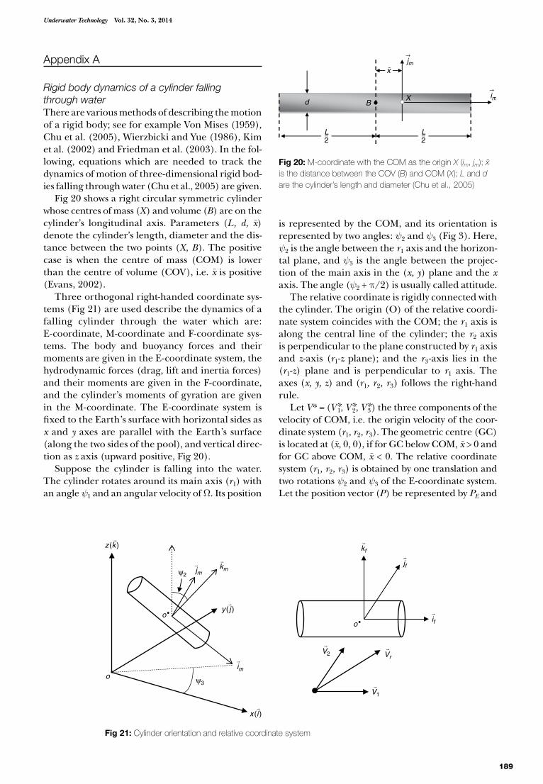
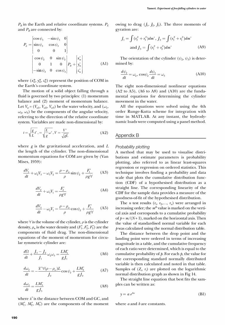