Nonlinear Modeling of Kinetic Plasma Instabilities

J. Candy�, H.L. Berk, B.N. Breizman and F. Porcelliy

Institute for Fusion Studies, The University of Texas at Austin, Austin, TX 78712

(January 20, 1999)

Abstract

Many kinetic plasma instabilities, in quite di�erent physical systems, share

a genuinely similar mathematical structure near isolated phase-space islands.

For this reason, dynamical features such as faster-than-exponential growth of

the instability, as well as nonlinear frequency sweeping, are found to be uni-

versal. Numerical �f methods, which follow the evolution of the (nonlinear)

perturbed distribution function along single-particle orbits, have been applied

to analytic models which include a continuous particle source, resonant par-

ticle collisions, and wave damping. The result is a series of codes which can

reliably model the nonlinear evolution of kinetic instabilities, including some

speci�c to tokamak plasmas, over experimentally relevant timescales. New re-

sults include: (i) nonlinear simulations of two-species, one-degree-of-freedom

plasmas; (ii) simulations of �shbone bursts in tokamak plasmas; (iii) nonlinear

modeling of beam-driven toroidal Alfv�en eigenmode activity in tokamaks.

Typeset using REVTEX

�present address: General Atomics, P.O. Box 85608, San Diego, CA 92186-5608

ypermanent address: Politecnico di Torino, 10129 TORINO, Italy.

1

I. INTRODUCTION

Bulk plasma instabilities, caused by the release of free energy by a population of energeticparticles, are commonly observed in modern tokamak plasmas. Toroidal Alfv�en eigenmodes(TAE) triggered by neutral beam injection [1,2] and ion-cyclotron resonance heating [3],alpha-driven TAE modes [4], and �shbone [5] modes are the best examples. In addition,energetic-particle-driven instabilities are found outside of mainstream tokamak physics aswell { the hot electron interchange mode in Terella [6], and collective modes in particleaccelerators [7].

Understanding the long-time nonlinear dynamics of these instabilities remains a dauntingtheoretical challenge. The presence of multiple disparate timescales makes a brute-forcenumerical simulation for many inverse growth times unrealistic if at all possible. For thisreason, simulations are often performed for only a relatively short time. These may entirelymiss long-time features of the instability observed in experiments.

We have made substantial progress on the rigorous treatment of the problem when thenonlinear dynamics is governed primarily by resonances which produce only isolated �rst-order phase-space islands (i.e., no overlapping of separatrices). Then, the e�ective Hamil-tonian for particles near each resonance has only one degree of freedom (two phase spacedimensions). We believe that the essential mechanisms for nonlinear saturation and fre-quency sweeping in many di�erent types of experiments are captured by our treatment.Remarkably, the physics can be described in its simplest form by studying the so-calledbump-on-tail instability.

For problems where the single-island approach may be insu�cient, we have developedsuitable particle codes. One such code is being developed to simulate TAE-induced beam-ion losses in tokamak plasmas such as TFTR [8] and DIII-D [9]. Results show that second-and higher-order islands may be important in understanding losses due to TAE bursts.

We have also carried out realistic simulations using a guiding center �shbone code whichuses a new operator technique [10,11] to include plasma diamagnetism and dissipation.With this, we are able to robustly reproduce the strong nonlinear frequency downshift ofprecessional modes, and have also clearly simulated explosive diamagnetic modes predictedby nonlinear theory [12]. A �shbone burst during a JET beam-heated discharge, withcore redistribution but no losses, has been numerically simulated. Simulation of larger,burning plasmas produce �shbone pulses, but with virtually insigni�cant core alpha particleredistribution. These results and their associated applicability conditions will be discussed.

II. FUNDAMENTAL EQUATIONS

We �rst describe the fundamental equations which govern the unstable mode evolutionand kinetic particle response. For simplicity, we will consider the case for which the mode isperturbative. A generalization of the procedure to the �shbone problem is made in Sec. V.

We write the real electric �eld of the mode as

~E(~r; t) = 2RehC(t)e�i!0t~e(~r; !0)

i; (1)

2

FIG. 1. Formation of a hole and clump in the energetic particle distribution for a system with

a single resonance. Here, �r = 0, L=!0 = 0:05, and d=!0 = �0:035. The vertical axis is n(I; t),

the density of particles as a function of action and time, obtained by integrating f over the angle,

�.

where !0 is the unperturbed frequency, C(t) is a slowly-varying complex amplitude, and~e(~r; !0) is the mode eigenvector. The frequency !0 is a solution of the linear dispersionrelation, excluding the energetic particle contribution and the dissipative part of the plasmaresponse. In Refs. [13,14] is it shown how to construct the equation governing the timeevolution of C(t). We �nd that, in terms of the distribution f of resonant particles, C(t)satis�es

�E d

dt+ d

!C(t) = q ei!0t

Zd�~e �(~r; !0) � ~v(�)f(�; t) ; (2)

with d the mode damping rate in the absence of energetic particles, EjCj2 the mode energy(up to a normalization factor), � = (~r; ~p) the phase space position, q the charge, and ~v thevelocity. This form of the evolution equation is su�ciently general to describe, for example,the nonlinear evolution of TAE modes in general plasma geometry. Eq. (2) for the (complex)amplitude, C(t), must be supplemented by a kinetic equation for f(�; t):

@f

@t+ [f;H] = C(f) +Q : (3)

Two forms of the collision operator are of interest; namely, a di�usive operator and aKrook operator. For the numerical modeling discussed in the present work, we use theKrook operator with source Q = �rf0 and annihilation rate �r

C(f) +Q = ��r(f � f0) ; (4)

3

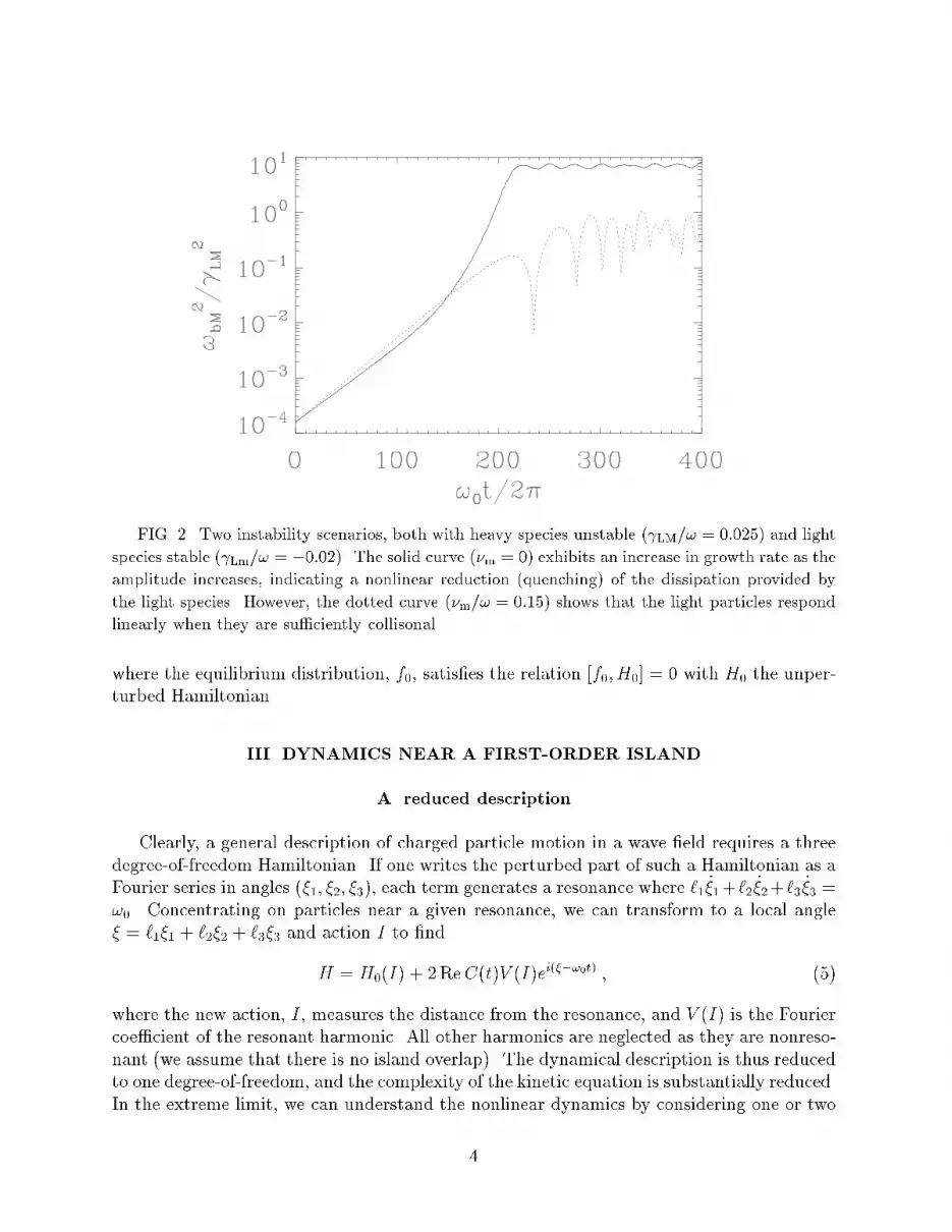
FIG. 2. Two instability scenarios, both with heavy species unstable ( LM=! = 0:025) and light

species stable ( Lm=! = �0:02). The solid curve (�m = 0) exhibits an increase in growth rate as the

amplitude increases, indicating a nonlinear reduction (quenching) of the dissipation provided by

the light species. However, the dotted curve (�m=! = 0:15) shows that the light particles respond

linearly when they are su�ciently collisonal.

where the equilibrium distribution, f0, satis�es the relation [f0; H0] = 0 with H0 the unper-turbed Hamiltonian.

III. DYNAMICS NEAR A FIRST-ORDER ISLAND

A. reduced description

Clearly, a general description of charged particle motion in a wave �eld requires a threedegree-of-freedom Hamiltonian. If one writes the perturbed part of such a Hamiltonian as aFourier series in angles (�1; �2; �3), each term generates a resonance where `1 _�1+`2 _�2+`3 _�3 =!0. Concentrating on particles near a given resonance, we can transform to a local angle� = `1�1 + `2�2 + `3�3 and action I to �nd

H = H0(I) + 2ReC(t)V (I)ei(��!0t) ; (5)

where the new action, I, measures the distance from the resonance, and V (I) is the Fouriercoe�cient of the resonant harmonic. All other harmonics are neglected as they are nonreso-nant (we assume that there is no island overlap). The dynamical description is thus reducedto one degree-of-freedom, and the complexity of the kinetic equation is substantially reduced.In the extreme limit, we can understand the nonlinear dynamics by considering one or two

4

FIG. 3. Spectral analysis for collisional case of Fig. 2. As expected, frequency sweeping occurs

when collisions make the reponse of the stabilizing light species nearly linear.

resonances as detailed in Sections III.b. and c. The numerical method used for these casesis based on a generalization of that presented in Ref. [15].

B. frequency sweeping e�ect

We �rst consider a one-dimensional electrostatic wave, where there is a single resonance!0� kv = 0. Numerical simulations [16] show that when an instability arises near threshold(i.e., = L� d � L, where L is the linear growth rate in the absence of dissipation) thelinear eigenfrequency !0 splits into individual spectral components that may shift upwardsand downwards in frequency. This splitting is connected with the emergence of a phase spacehole (the upshifted component) and/or a phase space clump (the downshifted component).Each nonlinear structure can be viewed as a Bernstein-Greene-Kruskal (BGK) mode [17].This phenomenon is illustrated in Fig. 1. Observe that the trough in the mean distributionmoves to higher velocity while the crest in the mean distribution moves to lower velocity.This behavior follows from the adiabatic invariance of trapped particle motion that causesthe trapped distribution to remain constant even as frequency changes. Thus, islands formin phase space with f -values substantially di�erent from the surrounding passing particledistribution. The higher velocity island is underpopulated and forms a hole, and the lowervelocity island is overpopulated and forms a clump. The motion of these islands allows freeenergy to be released from the unstable population to compensate for energy lost throughlinear dissipation [16].

5

C. two kinetic species

We have identi�ed an interesting phenomenon which arises when the model just presentedis modi�ed to include two populations of resonant particles { such that one population isstabilizing and the other destabilizing { and the extrinsic dissipation is set to zero.

First, consider the case when particles from the destabilizing population (henceforth,\light species", denoted by subscript m) have a smaller e�ective mass than particles fromthe stabilizing population (henceforth, \heavy species", denoted by subscriptM). This caseis not substantially di�erent from the previous one-species model. In particular, it exhibitsfrequency sweeping and the same saturation level. The reason for this similarity is that themode saturates when the trapping frequency of a light particle is comparable to Lm. Atthis level, the response of the heavy species is linear, since its trapping frequency is smallerby a factor of (m=M)1=2.

Now, if the heavy species is the destabilizing one, and the system is taken to be colli-sionless, quite a di�erent saturation process is observed. At su�ciently low amplitude, itis the stabilizing species that �rst experiences the dominant nonlinearity. In this case one�nds a \hard" instability, with explosive amplitude growth without oscillation or frequencysweeping. Unlike the case in which the stable species is heavy, the dissipation provided bya light stabilizing species nonlinearly quenches at an amplitude that is much less than thesaturation amplitude; namely Aquench � (m=M)Anat (see solid curve in Fig. 2). Here, Anat

is the expected, or \natural", saturation amplitude at which the trapping frequency of theunstable heavy species is comparable to the linear growth rate in the absence of dissipation.The quenching of the stabilization occurs because the trapping frequency of the stabilizingspecies exceeds the time rate of change of A, causing a plateau to form in the resonantphase space region of the stabilizing species. The �nal saturation level is close to that inthe undamped problem (!bM � 3 LM).

However, if in the previous scenario the light particles are su�ciently collisional (�r >�(M=m)1=2 LM), essentially linear dissipation may be recovered and the mode will again shiftin frequency. This is illustrated in Figs. 2 and 3. The saturation amplitude for the dottedcurve of Fig. 2, and the upshifted and downshifted spectral contours shown in Fig. 3 arenearly the same as those obtained when the dissipation is purely linear. In other simula-tions we have observed pronounced sweeping e�ects even when �r is appreciably less than(M=m)1=2 LM. This observation, namely that a su�ciently strong transport mechanism cansuppress nonlinearities from a stabilizing component, helps to justify the �shbone modellingdiscussed in the next section.

IV. FISHBONE OSCILLATIONS

A. nonperturbative formalism

Fishbones are unstable oscillations of the n = 1 internal kink mode, commonly observedin present-day tokamaks during neutral beam injection or ion cyclotron radio frequencyheating. Unlike the bump-on-tail instability we have discussed previously, �shbones [18]are generally nonperturbative modes; that is, they are not normal modes of the plasma

6

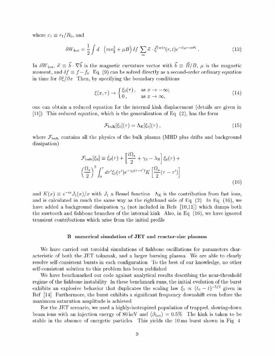
FIG. 4. Fishbone burst induced by 80 keV toroidally trapped beam ions in a JET-size plasma.

Only minor core redistribution results.

in the absence of energetic particles. In this case, the previous wave equation, Eq. (2), isinadequate.

To derive a suitable wave equation for the �shbone mode to replace Eq. (2), whichincludes the e�ects of plasma diamagnetism in the q = 1 layer, we summarize the derivationspresented in Refs. [10,11]. It is convenient to begin with the collisionless equation of motion

for the bulk plasma displacement ~�,

�Dtt~� =

1

c

��~|� ~B + ~| � � ~B

��r�pcore �r � �Phot ; (6)

where � is the mass density, Dtt is a di�erential operator that describes the e�ect of inertiaand �nite Larmor radius, ~| and �~| are the equilibrium and perturbed plasma currents, ~B and� ~B are the equilibrium and perturbed magnetic �elds, and �pcore is the perturbed (isotropic)pressure. The only nonlinear term is �Phot, the perturbed hot particle pressure tensor. Weemphasize that we consider no nonlinear MHD e�ects, a point that will be discussed further.It is standard to decompose the n = 1 displacement into a sum over poloidal components,~�(m),

~�(~r; t) =Xm

~�(m)(r; t)ei('�m�) + c.c. : (7)

We denote the radial component of ~�(1) by �, and let r1 be the radius of the q = 1 surface.The limiting form of the radial displacement is a step function, or \kink",

�(r; t) �!��0(t) ; if r < r1;0 ; if r > r1.

(8)

7

FIG. 5. Core redistribution corresponding to Fig. 4 at 12ms.

One can employ standard techniques to derive, from Eq. (6), a layer equation for thedisplacement (see Ref. [19] for the cylindrical limit and Ref. [20] for toroidal geometry). Thelayer equation can then be written in normalized variables, and integrated over the plasmaminor radius to give

@2

@� 2+ i�

@

@�+ x2

!@

@x�(x; � ) = S(� ) : (9)

Here, x � (r�r1)=r1 is the layer variable, � � !At is the normalized time, � � !�i=!A is thenormalized diamagnetic frequency, !�i = �(dpcore=dr)=(r�!ci) is the diamagnetic frequency(evaluated at the q = 1 surface), !A � vAs=

p3R0 is the Alfv�en frequency, vA = B0=

p4��

is the Alfv�en speed, s � d(ln q)=d(ln r) is the magnetic shear and R0 is the plasma majorradius. The integration constant S depends on outer layer physics only

S(� ) = ��H

��0(� )�

1

��K[�0](� ) : (10)

Here, �H is directly related to the minimized MHD potential energy

j�0(� )j2�H � � 2

(s"1B0)2�WMHD

R0

; (11)

and �K[�0](� ) represents the fast particle dynamics:

��0(� )�K[�0](� ) � � 2

(s"1B0)2�W hot(� )

R0

; (12)

8

where "1 � r1=R0, and

�W hot =1

2

Zd��mv2k + �B

��f

Xm

~� � ~�(m)�(r; t)e�i('�m�) : (13)

In �W hot, ~� � ~b � r~b is the magnetic curvature vector with ~b � ~B=B, � is the magneticmoment, and �f � f�f0. Eq. (9) can be solved directly as a second-order ordinary equationin time for @�=@x. Then, by specifying the boundary conditions

�(x; � )!��0(� ) ; as x! �1;0 ; as x!1,

(14)

one can obtain a reduced equation for the internal kink displacement (details are given in[11]). This reduced equation, which is the generalization of Eq. (2), has the form

Fbulk[�0](� ) = �K[�0](� ) ; (15)

where Fbulk contains all the physics of the bulk plasma (MHD plus drifts and backgrounddissipation)

Fbulk[�0] � _�0(� ) +�i�

2+ d � �H

��0(� ) +

��

2

�2 Z �

0d� 0�0(�

0)e� d(��� 0)K

��

2(� � � 0)

�(16)

and K(x) � e�ixJ1(x)=x with J1 a Bessel function. �K is the contribution from fast ions,and is calculated in much the same way as the righthand side of Eq. (2). In Eq. (16), wehave added a background dissipation d (not included in Refs. [10,11]) which damps boththe sawtooth and �shbone branches of the internal kink. Also, in Eq. (16), we have ignoredtransient contributions which arise from the initial pro�le.

B. numerical simulation of JET and reactor-size plasmas

We have carried out toroidal simulations of �shbone oscillations for parameters char-acteristic of both the JET tokamak, and a larger burning plasma. We are able to clearlyresolve self-consistent bursts in each con�guration. To the best of our knowledge, no otherself-consistent solution to this problem has been published.

We have benchmarked our code against analytical results describing the near-thresholdregime of the �shbone instability. In these benchmark runs, the initial evolution of the burstexhibits an explosive behavior that duplicates the scaling law �0 / (t0 � t)�5=2 given inRef. [14]. Furthermore, the burst exhibits a signi�cant frequency downshift even before themaximum saturation amplitude is achieved.

For the JET scenario, we used a highly-isotropized population of trapped, slowing-downbeam ions with an injection energy of 80 keV and h�fasti = 0:5%. The kink is taken to bestable in the absence of energetic particles. This yields the 10ms burst shown in Fig. 4.

9

FIG. 6. Fishbone burst caused by 3:5MeV trapped alphas in reactor-size plasma. There is

insigni�cant core-alpha redistribution.

FIG. 7. Instantaneous frequency corresponding to Fig. 6, showing a substantial nonlinear down-

shift. Note the onset of a second pulse at t � 32ms.

10

Comparing the radial beam pro�le at t = 0ms and during the maximum kink amplitude att = 6ms (see Fig. 5), we �nd that there is only an outward redistribution of particles, with nobeam ion losses { typical of �shbone oscillations in JET. The saturation level of this mode,�=a � 0:04 (which corresponds to �=r1 � 0:07), is lower than the estimate �=r1 � 1:0 basedon dimensional analysis, and more work is needed to understand why this is so. Because ofthis low observed level, we can readily justify the MHD linearization assumption.

For a reactor-relevant scenario, we consider an large (R0 = 814 cm), high-�eld (B0 =5:7 T) plasma for which the kink is, as before, stable before the introduction of energeticparticles. With a volume-averaged thermonuclear alpha particle beta of 0:3%, the trappedalpha particles drive a 30ms burst (see Fig. 6). The burst is accompanied by a strongfrequency downshift (as is the case for the JET run). This is shown in Fig. 7. Before the endof the simulation, one �nds the onset of a second burst. This arises due to the reconstitutionof the alpha distribution through �nite collision frequency in the kinetic equation, Eq. (4).

The two �shbone simulations give similar signals, though in the JET run the dimen-sionless saturated amplitude is 20 times greater, and produces signi�cantly more relaxationof the radial pressure pro�le. More work is needed to understand the scalings that lead tothese di�erences.

This simulation indicates that large, high-�eld machines may be more resilient to�shbone-induced losses than JET, at least in the case where the �shbone instability arisesfrom an MHD-stable kink.

C. validity of the model

The model equations we solve numerically purport to explain the saturation and fre-quency sweeping characteristic of �shbone oscillations as due to nonlinearity of the fast-ionprecessional drift resonance. However, in this problem there are two competitive resonante�ects: (i) the destabilizing drift resonance of the fast ions; namely ! � !D;hot (the pre-cessional drift frequency of fast ions); and (ii) a uid resonance associated with the bulkplasma; namely ! � kkvA, with kk(r) = (n � m=q)=R. Our approach has been to assumethat the uid response is purely linear, and treat the energetic particle resonance nonlin-early. However, it has been noted [21] that if we treat the plasma as an ideal MHD uid, theratio of the MHD nonlinearity to the energetic particle nonlinearity is roughly (svA=!R)2 {a large number, since the �shbone frequency is much less than the shear Alfv�en frequency.Therefore, on the basis of ideal MHD, it appears that we should not neglect the MHD non-linearity. In fact, if important, we would need to describe an entirely di�erent dynamicalmodel for the nonlinear evolution.

However, in tokamak plasmas, turbulent di�usion may have an e�ect similar to the colli-sional response already discussed in Sec. III. Thus, if through di�usive e�ects the plasma cancross a magnetic island in a time short compared to the time to complete a bounce inside theisland, then indeed it would be appropriate to neglect the MHD nonlinearity. For a radialdisplacement � found in a simulation, we can estimate the di�usivity required to neglect theMHD nonlinearity. Given the MHD resonance function � !�kk(r)vA, the bounce period,

�B, in a magnetic island is estimated from �B � jvE d=drj�1=2, where vE is the ~E� ~B driftvelocity. Taking !� � vE, we �nd �B � (Rr=�svA!)

1=2, with s the magnetic shear at the

11

FIG. 8. Simulation of beam-bursting in TFTR plasma for n = 2; 3; 4 TAE modes. Field

amplitudes of all modes are shown together, with n = 4 reaching the greatest values.

q = 1 surface. Next, the time, �di� , required for plasma with a di�usivity D to cross a mag-netic island of width �r � vE �B is �di� � (�r)2=D, and so to neglect the MHD nonlinearitywe require �di� < �B. Thus, the di�usion coe�cient must satisfy D > !r1=2�3=2(!R=svA)

1=2.We note that the global plasma lifetime (energy con�nement) is anomalous, and if we assumethe same di�usive process describes di�usion past an island, then �E � a2=D. The MHDnonlinearity can be then be neglected if �E < (a=�)3=2(a=r)1=2(svA=!R)

1=2. In the experi-ments we consider, �E � 0:1 s, and in our simulations, �=a < 0:04. Thus, we estimate thatthe assumptions needed to justify the present model are just on the edge of being ful�lled.

V. TAE-INDUCED BEAM LOSS

Some years ago, experiments carried out in both TFTR [1] and DIII-D [2] revealed asharp decrease in neutron count coincident with TAE bursts during neutral beam injection.Typical bursts were very short, and separated by a quiescent period of about 3ms. Eachburst was also accompanied by the loss of a substantial fraction (10-15%) of the accumulatedbeam ions. The resulting beam energy con�nement time was substantially less than the beamslowing slowing down time due to electron drag.

Here we describe status of our attempts to simulate this phenomenon. In the simulationsit is necessary to make some simplifying assumptions to make the simulations computation-ally feasible. Thus we consider the limit of purely parallel beam injection, where the mag-netic moment is zero, and thereby save by a huge factor on the number of marker-particles(patches of phase space which follow particle trajectories) required to perform accurate sim-ulations. Particle loss in experiment is quite important, and it needs to be implemented

12

FIG. 9. Collapse of the pressure pro�le corresponding to pulses in Fig. 8.

in the simulation with care. However, direct marker loss is contrary to the logic of the�f method, which requires that the markers move as an incompressible mesh. One wayto prevent marker loss is to choose perturbed eigenfunctions that vanish somewhat awayfrom the edge. We can then infer real particle loss by observing the fast-ion density pro�le attening in the regions where the perturbed �elds are nonzero. Presently, we have includeda spatially uniform annihilation rate that alters the density of particles on a marker but notthe motion of the marker itself. In this way we are able to model particle losses.

We also need to mock-up particle drag, which is a very important physical e�ect in theexperiment but not easy to directly include in the present �f algorithm. We take an indirectapproach that is based on the transient solution [22,23] of the Fokker-Planck equation. Withthe beam source Sexp = I0 �(v�vb)=v2b , the distribution of slowing-down ions is approximately

f0(v; t) =I0�s

v3 + v3cH[t� �(v)�s] ; (17)

where

�(v) =1

3lnv3b + v3cv3 + v3c

: (18)

Here, vb is the beam injection velocity, vc is the crossover velocity (see Refs. [22,23]), andI0 is the source intensity. At time �� after the injection begins, the low-velocity edge ofthe experimental distribution has velocity v�, where �� = �(v�)�s. The high-velocity edgeis the injection velocity, v = vb. Since the beam con�nement time is substantially lessthan �s, we expect that v� will be a substantial fraction of vb. However, since we cannot

13

easily describe the slowing-down dynamically, we mock-up the scenario by choosing theunperturbed distribution to be f0 as given in Eq. (17), with v�=vb � 0:7. This choiceensures that the velocity distribution in our simulation is similiar to what develops in theexperiments we are trying to explain. Then, the full distribution, f (which evolves accordingto TAE activity), is relaxed to f0 at a rate �r. This relaxation rate is adjusted to obtainpulsations at time intervals similar to those seen in experiment.

The kinetic equation for the simulated dynamics is

df

dt= �r(f0 � f) ; (19)

so that the strength of the beam source is not Sexp, but Ssim = �rf0. The e�ective powerintroduced into the plasma using our relaxation method can be related to the experimentalpower connected with the source Sexp. To a good approximation, we have

Psim

Pexp

=1

2�r�s

v2b � v2�v2b

: (20)

In this way we can compare the power input during the simulation with the experimentalvalue. Fig. 8 shows a simulation with three pulses; the second and third pulses separated byroughly 3ms. The collapse of the pressure pro�le, subsequent build-up, and further collapseduring the later pulse is clearly illustrated in Fig. 9. The beam power in this simulation is24MW { about 2-3 times the experimental value, and the peak amplitudes of the wave areroughly an order of magnitude higher than inferred from experiment. Thus these resultsindicate one possible mechanism for obtaining periodic pulses due to intense beam injection,but also indicate that additional physical processes need to be taken into account.

The pulsed losses observed in the TAE simulation may appear surprising since the �rst-order island treatment of Sec. III indicates that particle excursions are limited to the sizeof the island separatrix surrounding the resonance region, and that global di�usion doesnot occur outside the resonance region. However, the full nonlinear orbit-island structurecan facilitate global di�usion. This structure is illustrated in simpli�ed surface-of-sectionplots for which the �eld amplitude is �xed in time. In Fig. 10 we see a �rst order islandat r=a = 0:6. Within this island, phase space mixing leading to pro�le attenting willoccur. In addition, small higher-order islands exist, which create a stochastic region closerto the magnetic axis. When the nonlinear islands overlap, simulations exhibit an explosivebehavior, where di�usion caused by the growing nonlinear islands allows rapid conversionof particle free energy to wave energy. We see in Fig. 11 that at �B=B � 5 � 10�3, nearlythe entire phase space is stochastic. Only at the edge (r=a > 0:7), where we have arti�ciallylimited the �eld amplitude, is the particle motion regular. The large stochastic region causesa complete attening of the fast-ion density pro�le in the core. After attening, there is nomore free energy to release, and the wave damps due to any extrinsic linear damping. Aftera time t � 3ms, the pulse repeats, as the source and sinks rebuild the central density to thepoint where another collapse can occur.

At lower �eld amplitudes (�B=B < 10�3) higher order islands are not as important.However, global di�usion would still be possible if there are more linear modes excited thanwe had in these simulations. This can lead to an intermittent quasilinear scenario [24], in

14

FIG. 10. Surface of section for n = 4 TAE mode in TFTR plasma, showing presence of �rst,

second and third-order islands.

15

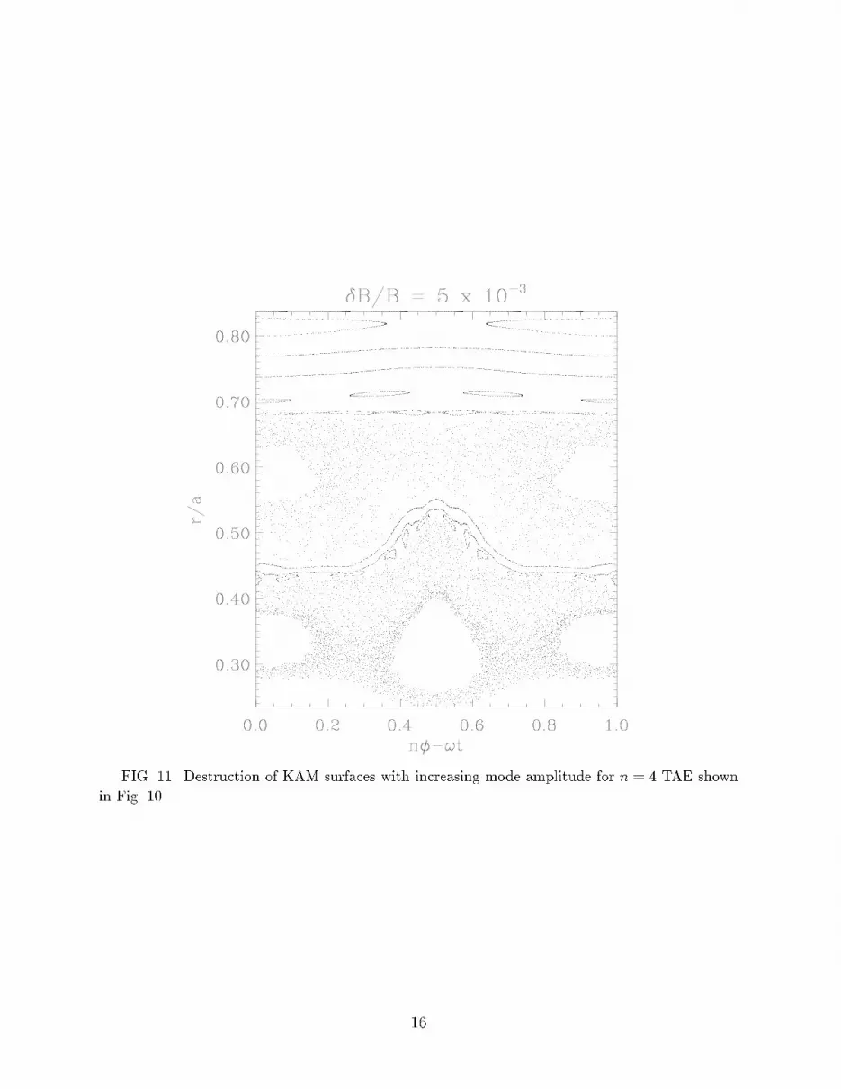
FIG. 11. Destruction of KAM surfaces with increasing mode amplitude for n = 4 TAE shown

in Fig. 10.

16

which lower level bursts of turbulence allow the system to hover close to the marginally stablestate without the complete collapse of the fast particle pressure pro�le. Also, additionale�ects of nonlinear mode coupling may limit the amplitudes of the bursts. Examining thesee�ects with the aim of reaching better agreement with the experimental data requires moreextensive numerical work.

VI. SUMMARY

In this paper, we have (i) described why the mathematical structure of kinetic instabilitiesis reducible to one-degree-of-freedom, and how consideration of simple models based onthis structure give insight into the behavior of instabilites in real devices; (ii) shown thata numerical model based on �rst-principles physical theory can realistically reproduce a�shbone burst typical for JET (for the cases studied, this model shows that �shbones causeless redistribution in a reactor than in JET-size devices); (iii) simulated TAE mode burstingin a TFTR-like plasma during neutral beam injection, and indicated how a fast collapseof the beam distribution during bursts may be caused by overlap of �rst- and higher-orderislands.

In the case of the �shbone simulations, there is still the need to verify the generality ofour observations with a more systematic scan of parameters and to intuitively understandwhy the relative saturation amplitude, �0=a, is so small.

Also, additional enhancements to the nonlinear TAE model in (iii) (including a morecareful treatment of particle losses and a more accurate reproduction of linear eigenmodes)are required to better replicate experimental data.

17

REFERENCES

[1] K.L. Wong, R.J. Fonck, S.F. Paul, et al., Phys. Rev. Lett. 66 1874 (1991).[2] W.W. Heidbrink, E.J. Strait, E. Doyle, and R. Snider, Nucl. Fusion 31 1635 (1991).[3] K.L. Wong, R. Majeski, M. Petrov, et al., Phys. Plasmas 4, 393 (1997).[4] R. Nazikian, G.Y. Fu, S.H. Batha, et al., Phys. Rev. Lett. 78 2976 (1997).[5] K.C. McGuire, R. Goldston, M. Bell, et al., Phys. Rev. Lett. 50 891 (1983).[6] H.P. Warren and M.E. Mauel, Phys. Plasmas 2 4185 (1996).[7] G.V. Stupakov, B.N. Breizman, and M.S. Pekker, Phys. Rev. E 55 5976 (1997).[8] D.M. Meade, V. Arunasalam, C.W. Barnes, et al., Proceedings 13th International Con-

ference on Plasma Physics and Controlled Fusion Research, Washington, DC, 1991

(International Atomic Energy Agency, Vienna, 1991), Vol. 1, 9.[9] J.L. Luxon and L.G. Davis, Fusion Technol. 8 441 (1985).[10] J. Candy, F. Porcelli, B.N. Breizman and H.L. Berk, Proc. 24th EPS Conf. Berchtes-

gaden (European Physical Society, Petit-Lancy, 1997), Vol. 21A III, 1189.[11] B.N. Breizman, J. Candy, F. Porcelli and H.L. Berk, Phys. Plasmas, Phys. Plasmas 5

2326 (1998).[12] J. Candy, H.L. Berk, B.N. Breizman and F. Porcelli, \Nonlinear Theory of Internal

Kink Modes Destabilized by Fast Ions in Tokamak Plasmas", Proc. 25th EPS Conf.Prague, Europhysics Conference Abstracts, Volume 22C, page 2141 (1998).

[13] H.L. Berk, B.N. Breizman, M.S. Pekker, Phys. Rev. Lett. 76 1256 (1996).[14] H.L. Berk, B.N. Breizman, and M.S. Pekker, Plasma Phys. Rep. 9 778 (1997).[15] J. Candy, J. Comput. Phys. 129 160 (1996).[16] H.L. Berk, B.N. Breizman, and N.V. Petviashvili, Phys. Lett. A 234 213 (1997).[17] I.B. Bernstein, J.M. Greene, and M.D. Kruskal, Phys. Rev. 108, 546 (1957).[18] L. Chen, R.B. White, and M.N. Rosenbluth, Phys. Rev. Lett. 52 1122 (1984).[19] M.N. Rosenbluth , R.Y. Dagazian, and P.H. Rutherford, Phys. Fluids 16 1894 (1973).[20] G.B. Crew and J.J. Ramos, Phys. Fluids 26 2621 (1983).[21] V. Pastukhov, B. Breizman, M. Pekker, and N. Chudin, Bull. Am. Phys. Soc. 43 1753

(1998).[22] H.L. Berk, W. Horton, M.N. Rosenbluth and P.H. Rutherford, Nucl. Fusion 15 819

(1975).[23] J.D. Ga�ey, J. Plasma Phys. 16 149 (1976).[24] H.L. Berk and B.N. Breizman, \Overview of Nonlinear Theory of Kinetically Driven

Instabilities," IFSR Report #841 (to be published in Theory of Fusion Plasmas, 1998,ed. M.J. Vaclavik and E. Sindoni, Italian Physics Society, Bologna Italy).

18