713

Theoretical analysis of Poiseuille flow instabilitiesin nematics

P. Manneville

Service de Physique du Solide et de Résonance Magnétique,Orme des Merisiers, B.P. n° 2, 91190 Gif sur Yvette, France

(Reçu le 19 décembre 1978, accepté le 5 mars 1979)

Résumé. 2014 Nous étudions la stabilité de l’écoulement de Poiseuille dans un nématique en géométrie planaire.Nous prolongeons l’analyse de la référence [5] pour tenir compte des distorsions périodiques du directeur. Plu-sieurs approches différentes sont mises en 0153uvre : modèles simplifiés, méthode de Galerkin ou simulation numé-rique. Nos résultats permettent d’interpréter l’ensemble des données expérimentales obtenues jusqu’à présent(réfs. [4] et [9]).Abstract. 2014 We study the stability of a Poiseuille flow in a planar nematic. We extend the analysis given in ref. [5]to take into account periodic distortions of the director. Several different approaches are employed : simplifiedmodels, Galerkin method, or numerical simulation. Our results allow one to interpret experimental findings sofar obtained (refs. [4] and [9]).

LE JOURNAL DE PHYSIQUE TOME 40, JUILLET 1979,

Classification

Physics Abstracts47.15F

1. Introduction. - Recently much attention hasbeen devoted to hydrodynamic instabilities in NematicLiquid Crystals [1]. A situation of particular interestis achieved when the mean molecular orientation is

perpendicular to the shearing plane [2]. Instabilitieswhich set in then result from the very specific couplingbetween the velocity field and the director ; theyoccur at very low Reynolds numbers. The case ofthe Simple Shear Flow (S.S.F. in the following) is

pretty well understood [3]. Steady as well as alter-nating flows have been investigated and the effectsof applied electric and magnetic fields have beenexamined. Two different instability modes can takeplace : a uniform distortion called the HomogeneousInstability (H.I.) and a periodic distortion, the RollInstability (R.L). Essential parameters are the signof a3, the intensity of the external fields and/or thefrequency. When a3 > 0 only the R.I. can take

place. When a3 0, the H.I. which sets in at lowfield/frequency is replaced by the R.I. at high field/fre-quency. Quantitative agreement between experimentsand theory is quite satisfactory.

Before a complete understanding of the S.S.F.instabilities was obtained, planar Poiseuille flow

began to be investigated. The first experimentalresults were qualitatively accounted for by a modelin terms of an assemblage of average simple shearflows [4] but the detailed theoretical analysis tumed

out to be far more difficult. First results obtainedconcemed the symmetry properties of the unstablemodes (which lead to a useful classification of expe-rimental facts) and the detailed solution of the steadyflow H.I. [5] in complete agreement with experiments.However experiments revealed more complexitiesthan one could have inferred from the simple trans-position of the simple shear flow case and muchremained to be accounted for.

In this paper we intend to complete the theoreticalaccount of experiments. The main source of difficultyoriginates from the fact that the shearing rate of theprimary flow is no longer constant so that somecoefficients of the partial differential equations govern-ing the problem become variable. To cope with thisdifficulty we shall develop essentially three différentkinds of approach : approximate models, Galerkinanalysis or direct numerical integration. Detailedcalculations are rather lengthy and tedious, so theywill be skipped over since they have been reportedelsewhere [6]. Notations and general equations havealready been given [7] and will not be repeated here.The paper is organized as follows :- In section 2, we recall the symmetry of the

unstable modes and the solution of the steady flowHomogeneous Instability. We take advantage of itssimplicity to check the prototype of approximatemodels to be used in other sections.

Article published online by EDP Sciences and available at http://dx.doi.org/10.1051/jphys:01979004007071300

714

- Section 3 is devoted to the effect of externalfields on homogeneous as well as periodic instabilitymodes.- Then thé analysis is extended to altemating

flows (§ 4). Specific features of the stability analysisand additional symmetry properties are briefly dis-cussed. Then we consider the altemating Homoge-neous Instability which is solved by direct numericalintegration. The case of rolls is discussed within theframework of an approximate model derived fromthat presented in § 2.- Finally, agreement between experiments and

theory is examined in section 5, and prospects forfuture work are suggested.Now, before we begin by recalling previous results,

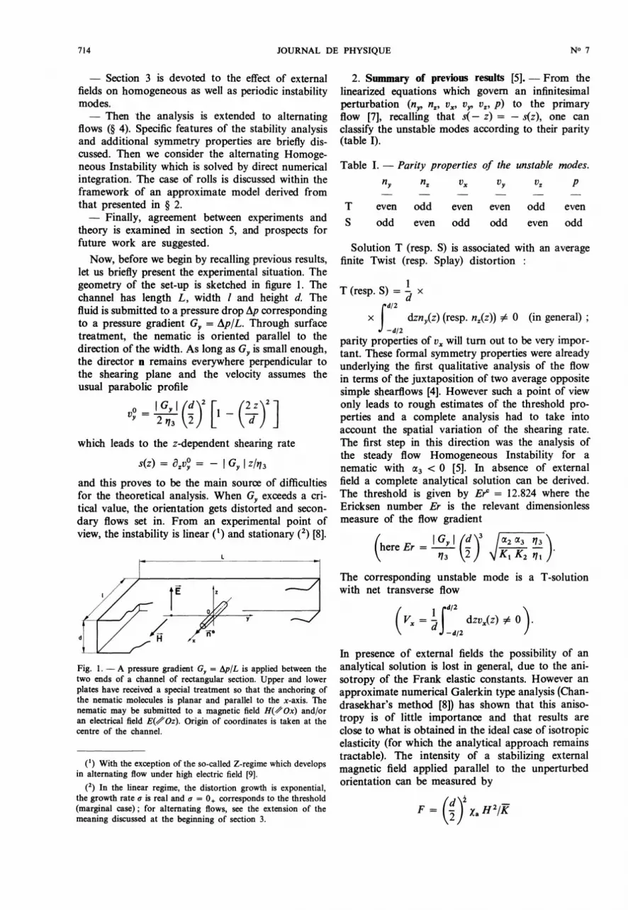
let us briefly present the experimental situation. Thegeometry of the set-up is sketched in figure 1. Thechannel has length L, width 1 and height d. Thefluid is submitted to a pressure drop Ap correspondingto a pressure gradient Gy = Ap/L. Through surfacetreatment, the nematic is oriented parallel to thedirection of the width. As long as Gy is small enough,the director n remains everywhere perpendicular tothe shearing plane and the velocity assumes theusual parabolic profile

which leads to the z-dependent shearing rate

and this proves to be the main source of difficultiesfor the theoretical analysis. When Gy exceeds a cri-tical value, the orientation gets distorted and secon-dary flows set in. From an experimental point ofview, the instability is linear (1) and stationary (2) [8].

Fig. 1. - A pressure gradient Gy = àplL is applied between thetwo ends of a channel of rectangular section. Upper and lowerplates have received a special treatment so that the anchoring ofthe nematic molecules is planar and parallel to the x-axis. Thenematic may be submitted to a magnetic field H(//Ox) and/oran electrical field EifOz). Origin of coordinates is taken at thecentre of the channel.

(1) With the exception of the so-called Z-regime which developsin alternating flow under high electric field [9].

(2) In the linear regime, the distortion growth is exponential,the growth rate a is real and a = 0+ corresponds to the threshold(marginal case) ; for alternating flows, see the extension of the

meaning discussed at the beginning of section 3.

2. Summary of previous results [5]. - From thelinearized equations which govem an infinitesimalperturbation (nY’ nz, vx, VY’ vZ, p) to the primaryflow [7], recalling that s( - z) = 2013 s(z), one can

classify the unstable modes according to their parity(table I).

Table I. - Parity properties of the unstable modes.

Solution T (resp. S) is associated with an averagefinite Twist (resp. Splay) distortion :

parity properties of vx will tum out to be very impor-tant. These formal symmetry properties were alreadyunderlying the first qualitative analysis of the flowin terms of the juxtaposition of two average oppositesimple shearflows [4]. However such a point of viewonly leads to rough estimates of the threshold pro-perties and a complete analysis had to take intoaccount the spatial variation of the shearing rate.

The first step in this direction was the analysis ofthe steady flow Homogeneous Instability for a

nematic with a3 0 [5]. In absence of externalfield a complete analytical solution can be derived.The threshold is given by Erc = 12.824 where theEricksen number Er is the relevant dimensionlessmeasure of the flow gradient

The corresponding unstable mode is a T-solutionwith net transverse flow

In presence of external fields the possibility of ananalytical solution is lost in general, due to the ani-sotropy of the Frank elastic constants. However an

approximate numerical Galerkin type analysis (Chan-drasekhar’s method [8]) has shown that this aniso-tropy is of little importance and that results are

close to what is obtained in the ideal case of isotropicelasticity (for which the analytical approach remainstractable). The intensity of a stabilizing extemal

magnetic field applied parallel to the unperturbedorientation can be measured by

715

which expresses the ratio of the magnetic torque tothe elastic one (K is some average value for theFrank constant). The variation of the threshold withthe field is given by

Contrary to what was first thought, such a peculiarvariation can in fact easily be derived from a sim-plified model that we shall develop here, since weshall refer to it in section 3 and 4. Let us considerfigure 2a which presents the fluctuation profile ofthe T-distortion at high fields (F = 150). In thecentral part (z - 0) where the shearing rate is small,the distortion is small due to the stabilizing effectof the field. On the contrary in the neighbourhoodof the plates (z - ± d/2) the Pieranski-Guyon insta-bility mechanism leads to a large distortion. Thisstrongly suggests the simplified distortion depictedon figure 2b where a stable central layer is assumedto separate unstable layers of thickness ô (0 ô « d/2)close to the plates. The distortion is taken of the form

Fig. 2a. - Solution of the exact calculation : in the central regionthe distortion is very small due to the stabilizing effect of the fieldwhile the destabilizing mechanism proportional to the square ofthe shearing rate is very weak.

Fig. 2b. - Approximate model describing the situation of

figure 2a : two unstable layers of thickness ô are submitted to anaverage simple shear + 37(ô). Optimizing ô leads to an excellentagreement with the exact calculation.

Fig. 2. - Fluctuation profiles under large fields (hereF = la H2 d2/4 K ~ 150) for the homogeneous instability dis-cussed in ref. [5].

where ç represents the distance to the plate, andthe unstable layers are submitted to an average shear

The instability criterion is then given by the SimpleShear flow theory [7]

in which b is still a free parameter. The threshold isthen given by the value bc which minimizes the

critical shear. Turning to dimensionless notations,with L1 = 2 b/d one gets (2) in the form

The extremum condition DErlôd = 0 reads

and when F is large the root of eq. (3) is approximatelygiven by

so that

in excellent agreement with the analytical result (1)which we can write Erc =F + 2.338 F 2/3 + 0 (Fl/3).

Let us take the opportunity to stress the factthat Li (or 03B4) is not a coherence length as it is definedfor exemple in the Freedericks problem [10]. In thatcase the coherence length is directly related to thebalance between the magnetic torque and the elasticone when surface effects and field effects are con-

flicting : this leads to l5 ’" 1 / H. In the present case,these effects are not conflicting but both strugglewith the destabilizing mechanism, which leads to amore involved compromise and to the rather strangedependence à - H-2/3 : a simple dimensional argu-ment based on the Freedericks coherence length(irrelevant to the present problem) would fail.

3. Steady Poiseuille flow : general approach. - Inthe simple shear flow case the uniform distortioncorresponding to the Homogeneous Instability cantake place at low fields when a3 is negative. At higherfields a distortion sets in which is periodic in thedirection of the unperturbed orientation, this dis-tortion is associated with a secondary flow in formof rolls, the order of magnitude of the wavelengthbeing given by the thickness of the unstable layer.Recalling the analogy between a Poiseuille flowand two juxtaposed simple shear flows one expects

716

such a roll instability to be possible (Fig. 3) and onecan estimate the cross-over field from the H.I. tothe R.I. Even at fields much larger than this estimatedcross-over field and at least for steady flows such atransition has not been observed experimentallywhich clearly needs an explanation. The origin ofthe discrepancy can be traced back to the couplingboth elastic and viscous between the upper and lowerhalves of the channel which must alter the simplepicture of Poiseuille flow in terms of decoupledunstable layers submitted to average simple shears.Unfortunately a quantitative account of this effectleads to a cumbersome analysis. The normal modeanalysis developed for the simple shear case [7] nolonger works due to the z-dependence of the shearingrate and one must turn to a Galerkin approach(Chandrasekhar’s method [8]) derived from thatoutlined in ref. [5] for the Homogeneous Instability.Calculations result in the determination of the

complete curve of marginal stability i.e. the critical

pressure drop (or Ericksen number) as a functionof the wave vector q,, of the periodic distortion.

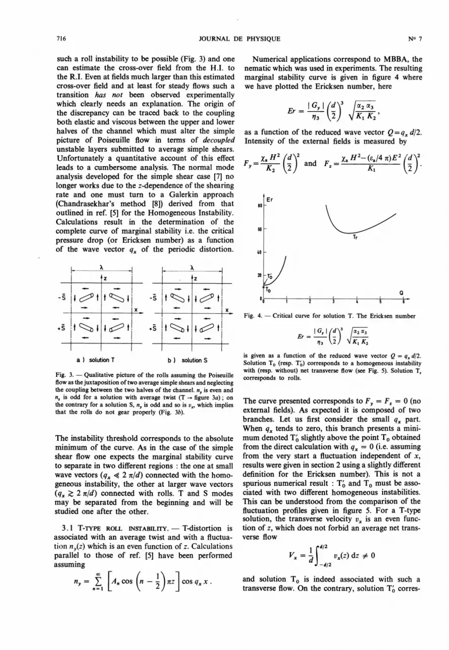
Fig. 3. - Qualitative picture of the rolls assuming the Poiseuilleflow as the juxtaposition of two average simple shears and neglectingthe coupling between the two halves of the channel. ny is even andn., is odd for a solution with average twist (T --> figure 3a) ; onthe contrary for a solution S, ny is odd and so is v.,, which impliesthat the rolls do not gear properly (Fig. 3b).

The instability threshold corresponds to the absoluteminimum of the curve. As in the case of the simpleshear flow one expects the marginal stability curveto separate in two different regions : the one at smallwave vectors (q. « 2 03C0/d ) connected with the homo-geneous instability, the other at larger wave vectors(qx > 2 nid) connected with rolls. T and S modes

may be separated from the beginning and will bestudied one after the other.

3.1 T-TYPE ROLL INSTABILITY. - T-distortion isassociated with an average twist and with a fluctua-tion ny(z) which is an even function of z. Calculationsparallel to those of ref. [5] have been performedassuming

Numerical applications correspond to MBBA, thenematic which was used in experiments. The resultingmarginal stability curve is given in figure 4 wherewe have plotted the Ericksen number, here

as a function of the reduced wave vector Q = qx d/2.Intensity of the external fields is measured by

Fig. 4. - Critical curve for solution T. The Ericksen number

is given as a function of the reduced wave vector Q = qx dJ2.Solution To (resp. Te) corresponds to a homogeneous instabilitywith (resp. without) net transverse flow (see Fig. 5). Solution T,corresponds to rolls.

The curve presented corresponds to Fy = F, = 0 (noexternal fields). As expected it is composed of twobranches. Let us first consider the small qx part.When qx tends to zero, this branch presents a mini-mum denoted To slightly above the point To obtainedfrom the direct calculation with qx = 0 (i.e. assumingfrom the very start a fluctuation independent of x,results were given in section 2 using a slightly differentdefinition for the Ericksen number). This is not a

spurious numerical result : To and To must be asso-ciated with two different homogeneous instabilities.This can be understood from the comparison of thefluctuation profiles given in figure 5. For a T-typesolution, the transverse velocity vx is an even func-tion of z, which does not forbid an average net trans-verse flow

and solution To is indeed associated with such atransverse flow. On the contrary, solution T 0 corres-

717

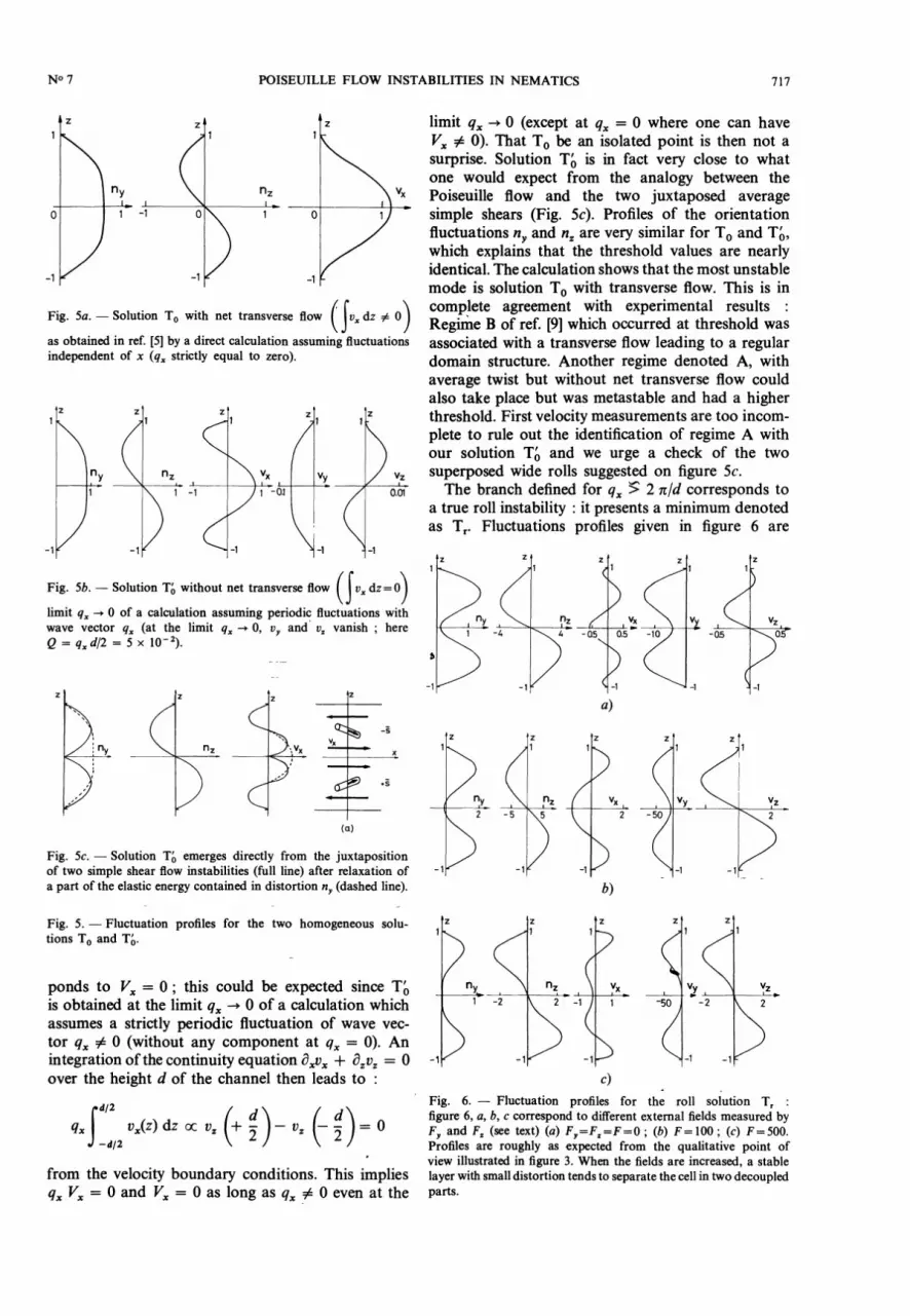
Fig. 5a. - Solution To with net transverse now ( ) VX dz # 0as obtained in ref. [5] by a direct calculation assuming fluctuationsindependent of x (q x strictly equal to zero).

Fig. 5b. - Solution To without net transverse flow (J vx dz=0 )limit qx ---> 0 of a calculation assuming periodic fluctuations withwave vector qx (at the limit qx -> 0, vy and vz vanish ; here

Fig. 5c. - Solution To emerges directly from the juxtapositionof two simple shear flow instabilities (full line) after relaxation ofa part of the elastic energy contained in distortion ny (dashed line).

Fig. 5. - Fluctuation profiles for the two homogeneous solu-tions To and T..

ponds to Yx = 0 ; this could be expected since Toiis obtained at the limit qx -+ 0 of a calculation whichassumes a strictly periodic fluctuation of wave vec-tor q,, :0 0 (without any component at qx = 0). Anintegration of the continuity equation ôxvx + ôzvz = 0over the height d of the channel then leads to :

from the velocity boundary conditions. This impliesqx Vx = 0 and Vx = 0 as long as qx = 0 even at the

limit qx --> 0 (except at qx = 0 where one can haveV" =1= 0). That To be an isolated point is then not asurprise. Solution To is in fact very close to whatone would expect from the analogy between thePoiseuille flow and the two juxtaposed averagesimple shears (Fig. 5c). Profiles of the orientationfluctuations ny and nz are very similar for To and TO,which explains that the threshold values are nearlyidentical. The calculation shows that the most unstablemode is solution To with transverse flow. This is incomplete agreement with experimental results :

Regime B of ref. [9] which occurred at threshold wasassociated with a transverse flow leading to a regulardomain structure. Another regime denoted A, withaverage twist but without net transverse flow couldalso take place but was metastable and had a higherthreshold. First velocity measurements are too incom-plete to rule out the identification of regime A withour solution To and we urge a check of the twosuperposed wide rolls suggested on figure 5c.The branch defined for qx > 2 nld corresponds to

a true roll instability : it presents a minimum denotedas Tr. Fluctuations profiles given in figure 6 are

Fig. 6. - Fluctuation profiles for the roll solution T r :figure 6, a, b, c correspond to different external fields measured byFy and F% (see text) (a) Fy =FZ =F = 0 ; (b) F =100 ; (c) F = 500.Profiles are roughly as expected from the qualitative point ofview illustrated in figure 3. When the fields are increased, a stablelayer with small distortion tends to separate the cell in two decoupledparts.

718

roughly as expected from the naive sketch (Fig. 3a).Upper and lower halves of the channel are ratheruncoupled and a stable layer appear in the centralpart (z - 0) with increasing fields. Evolution of theinstability threshold with external fields is givenin figure 7 for the three T-solutions. One can see thatthe homogeneous instability with transverse flow Tohas always the lowest critical value and that if it didnot exist one would observe the cross-over from Toito Tr exactly as in the simple shear case.

Fig. 7. - Threshold of the three different solutions with averagetwist as a function of external fields.

3.2 S-TYPE ROLL INSTABILITY. - A distortion with

average splay corresponds to a fluctuation n,(z)which is an odd function of z, so that the calculationhas been performed assuming

Figure 9 displays marginal stability curves forseveral values of the extemal fields. The two branchesat small and large qx only appear for large enoughextemal fields. This can be understood from the

qualitative picture of figure 3b. Indeed an S-typesolution involves an odd transverse velocity ux and

Fig. 9. - Fluctuation profiles for solution S, ; (a) F = 100, thesituation is still far from what was expected in figure 3b. (b) F = 500the two halves of the channel are rather decoupled by the stablelayer, distortions begin to concentrate close to the plate, apartfrom parity profiles look like those given in figure 6c for rolls Tr.

Fig. 8. - S-critical curves for different values of external fields. Rolls can take place only if F is large enough.

719

a strong velocity gradient ôzvx in the mid-plane (z = 0) ;in other words, rolls do not gear correctly. Distor-tions in the upper and lower halves of the channelare so strongly coupled that a roll instability with awave vector of the order of 2 n/d cannot exist inzero field. With increasing field, the role of the centrallayer (z - 0) weakens and a roll instability can

exist. At moderate fields, fluctuation profiles are

still far from what one expects (Fig. 9a) but thesituation gets better at higher fields and the twohalves of the channel become uncoupled (Fig. 9b).

Let us now tum to the small qx part of the curve.On the enlargement given in figure 10 for Fy = Fz = 0,one first notices that the minimum does not take

place at qx = 0 but rather at Q = qx d/2 - 1 so thatthe homogeneous S-type instability studied in ref. [5]and denoted here as So is in fact unstable against aroll fluctuation of long wavelength (since v., is odd,the net transverse flow is zero and the discontinuityat qx = 0 does not appear). Figure 11 displays thefluctuation profiles at So and at the minimum of thecurve. vx and ny are quite similar and the fact that Solies slightly above the minimum is to be related tothe shape of nz. Indeed the dominant part of the

elastic ener gY is 12 K1 J (Oz:nz)2 dz and when n z getsmore regular, this energy gets smaller and the insta-bility threshold decreases. In the following we shalldenote the minimum of the curve So to recall thatit occurs at small wave vectors (index 0) and origi-nates from the relaxation of a part of the elastic

energy contained in solution So. It should be notedhere that calculations have been performed usingvalues of the viscoelastic coefficients for MBBAtabulated in ref. [10] (with a3/a2 = 1.53 x 10-2) ;

Fig. 10. - Enlargement of the small qx part of the curve F = 0given in figure 8. Solution So discussed in ref. [5] is in fact a relativemaximum of the critical curve. The threshold takes place at Q N 1

(solution Sô) however the critical value of the homogeneous solutionwith transverse flow To lies below that for S..

Fig. 11. - Fluctuation profiles for S-type solutions at small wavevectors. The difference between solution So (Q = 0, figure lla)and So (Q N 1 ; figure l lb) is obvious for fluctuation n., whichlooks like cos (nzld) for S, while ny and vx bear nearly no change.The contribution of vy is not negligible when Q - 1 and shouldbe taken into account in the discussion of the mechanism for S..

for slightly larger a3 (a3Ia2 > 4 x 10-2) (3) So tendstowards So which becomes a true minimum insteadof being an unstable relative maximum.As can be seen in figure 10, So remains above To

so that the homogeneous T-instability with transverseflow is expected at threshold in agreement with

experiments [4, 9]. Now let us recall that in theirfirst series of experiments [4] Pieranski and Guyonhave observed in the non-linear regime above thethreshold of the To-mode a roll instability of theS-type with a wavelength 2 or 3 times the thicknessof the cell which has all the characteristics of our

solution When

one increases the external fields the critical valuefor So and To remain very close to each other. UsingGâhwiller’s viscosity values one can even predict across-over from To to So which is not observed

experimentally. The reason may be that To is observedin a metastable state due to the operating procedurebut more probably that temperature or impurityeffects lead to a slightly different set of viscoelasticcoefficients. Indeed changing a3/a2 from 1.53 x 10- 2to 2.5 x 10-2 is sufficient for the mode To to remainthe most unstable one. This interpretation is rein-

(3) a3 is not a free parameter since it enters an Onsager relationbut as long as a3 remains small enough one can neglect the effectof its variation on other viscosity coefficients. Calculations havebeen performed keeping all viscoelastic coefficients constant

except a3.

720

forced by the fact that solution So has not beenobserved in the second series of experiments [9],indicating slightly different experimental conditions.The great sensitivity of the result to the exact

value of a3 has led us to reexamine the instabilitymechanism of this particular solution So. Let usassume a long wavelength distortion nz extending overthe whole thickness of the channel (see Fig. llb)

such a distortion induces a viscous torque [2, 7]

which tends to make the director rotate so that afluctuation ny appears. when qx = 0 one recoversthe original Pieranski-Guyon mechanism for a homo-geneous instability [2] corrected to take secondaryflow effects into account [7] ; namely, viscous forcesinduce a transverse flow vx which adds its contri-bution - a3 ô,,,,v. to the viscous torque created bythe fluctuation ny

when a3 is negative this tends to increase the distor-tion nz. Now when qx "# 0, due to the continuity ofthe fluid, the fluctuation vx induces a vertical velo-city Vz which contributes to the torque fy througha term - OE2 ôxvz (a2 0). A careful examinationof the global effect shows that the sequence sketchedbelow

Fig. 12. - Threshold of So as a function of oc3. Here

oc.3 is negative at high temperatures and may be positive belowsome inversion temperature while U2 remains negative. Noticethat a roll instability Tr can also exist, the threshold of which isnot much affected by a3 so that one could witness the cross-overfrom S, to Tr at another temperature somewhat below the inversiontemperature. Calculations have not been performed since detailedviscoelastic data are not available.

works in a destabilizing way as long as qx # 0 andsmall, whatever the value of a3 positive or negativeas long as a3 is small enough. So when a3 is positiveand small, the usual homogeneous instability Tocan no longer take place but So does. Figure 12

displays the threshold of the solution So for an

imaginary nematic which would have the same

viscoelastic coefficients as MBBA except for a

small and variable a3 (3). The reduced wave vectorQ = qx d/2 slowly varies with a3 from 0.8 for

CX3 = - 2.5 x 10-2, CX2 1 to 1.2 for CX3 = + 3.3 x 10-2 , CX2 1. .The result given above is not of academic interestsince there exist nematics for which a3 varies from

negative values close to the clearing point to positivevalues at lower temperatures, in connection with atendency to smectic ordering. These nematics will

present a cross-over from a solution To to the longwavelength splay distortion So when the temperatureis lowered.

3. 3 REMARK : : ASYMPTOTIC REGIME FOR ROLLS

UNDER HIGH FIELDS. - Despite the fact that rollsare always masked either by a homogeneous insta-bility To or by solution S’, let us consider the asymp-totic behaviour of rolls under high fields. It is obtainedthrough an extension of the model of section 2 whichcombines the idea of unstable layers with results ofthe simple shear flow instability theory [3] : for rolls,exact results are well accounted for by an approximatenormal mode analysis which rests on effective torqueequations and assumes a simplified analytical formfor the fluctuations. Here :

where ç is again the distance to the upper and lowerplates, and q., is taken as 03C0/03B4, ô being the thicknessof the unstable layer submitted to the average shears(b). At the limit of high fields and large wave vec-tors (q2x > q2z) with notations of ref. [3] the criticalcondition reads

à (through qz, and -s) and qx are two parameters tobe optimized, the threshold corresponding to thelowest critical value. With L1 and F as defined insection 2 and

eq. (4) reads

721

Extremum conditions ôEr/64 = 0 andlead to

Elimination of F gives

which relates the wave vector to the unstable layerthickness. In the limit R > 1 and 4 « 1 this maybe simplified to

the optimum layer thickness is then given by eq. (5)

so that

As can be seen in figure 13 this asymptotic behaviouris fairly well verified by solution Tr as calculatedfrom the Galerkin expansion. As already stated, thedecoupling between the upper and lower half of thechannel is more difficult to obtain for S-type rolls,so that agreement with the asymptotic line onlyappears for the highest calculated points. This factalso explains that threshold values for S, are about10 % higher than those for T, (Fig. 14). Of coursesuch a difference is not accounted for by the simplifiedmodel which does not separate solutions of différent

parities. Finally from (4) and (5’) one deduce

Contrary to the case of the Homogeneous Insta-bility, coefficients entering this expansion are very

, difficult to estimate and (6) rather gives a generaltrend of evolution which may help to analyse data

Fig. 13. - An indication of the validity of the approximate modelfor rolls under large fields is given by the behaviour of the wavevector Q - F 3/8. Dots and crosses correspond to calculated valuesfor Tr and Sr respectively.

Fig. 14. - The threshold for rolls with average twist (T,) liesabout 10 % below that for rolls with average slay (S,).

on roll instabilities (see below the alternating flowcase).

4. Alternating Poiseuille flows. - From a concep-tual point of view it is not difficult to extend thelinear stability analysis from the case of a steadyflow to that of an alternating one ( 11 ] . In the firstcase one looked for solutions of a differential systemwith coefficients independent of time under theform w(r, t) = w(r) exp ut ; marginal stability cor-

responding to Re { a} = 0 and the exchange ofstabilities to Im { a } = 0 at threshold [8]. In the

case of a periodic basic flow of period T certaincoefficients of the differential system become time-dependent and one cannot eliminate the temporaldependence through a simple exponential factor. Asin the case of ordinary differential equations, oneassumes a kind of Floquet separation [12]

where w is periodic in t with period T. The expo-nential factor now describes the evolution of thefluctuation once the variation forced by the basicflow has been substracted. Again the instabilitysets in when Re { a } > 0. Condition Im { Q } = 0at threshold now corresponds to an extension ofthe hypothesis of exchange of stabilities ; it merelystates that the only period relevant to the problemis the one imposed from the outside. As in the caseof steady flows the validity of this assumption shouldbe checked rather than taken for granted. The sepa-ration of the temporal dependence in two parts is

particularly clear on figure 15 to be discussed further.The next step is to search for periodic solutions w

of the eigenvalue problem. At least formally this, can be performed through a Fourier expansion :

722

Fig. 15. - Time evolution for the numerical solution of the

Homogeneous Instability in square wave alternating flows. Tickson the time axis mark every reversal of the flow direction (reducedfrequency 1/T = (Y1 d2/4 Kl) f = 12.5). The upper (resp. lower)curves display the behaviour of ny (resp. nz). The 3 or 4 first periodscorrespond to an adjustment of the spatial profiles of ny and n,,from those given as initial conditions. Then an asymptotic regimeis reached where fluctuations grow (Er = 130 > Erc) or decay(Er = 90 Er°). We present the case of the Z-regime where nzchanges sign from one 1/2-period to the next. In the marginalcase Er = Er° N 120, the exponential trend disappears and one

is left with n. (t + T)= - nz(t) and ny periodic with period T/2.(t+ 2

Time dependent coefficients of the equations arealso expanded and after separation of the differentharmonics one gets an infinite system of equationswhere time is absent. Of course the solution is obtainedafter truncation at a sufficiently high order butfrom a practical point of view this program is hardlyachievable and one is lead to severe approximations.Before entering into details, let us point out thetemporal symmetry properties linked to the perio-dicity of the basic flow. In experiments square waveexcitation has been used which is such that

s(t + T/2) = - s(t) .

This allows to distinguish a Z-mode (nomenclatureof ref. [2]) where nz alternâtes from one half-periodto the next (nz(t + T/2) = - nz(t)) while ny doesnot (ny(t + T/2) = ny(t)) from a Y-mode where nyand nz exchange their role. Moreover the fluctuationwith the shortest natural relaxation time is expectedto oscillate. Classification of the unstable modes inthe Poiseuille problem then involves parity and

periodicity and one can expect four different regimesY-T, Z-T, Y-S, Z-S.

4.1 HOMOGENEOUS INSTABILITY. - The homoge-neous instability takes place at low frequencies.Even if the equations are much simpler in that casethan for rolls, the system has variable coefficientsin space and time and the Galerkin procedure hasto be performed on both variables. Moreover at

low frequencies the exact form of the excitation

square wave or sinusoid is important and many

harmonics must be retained (for a discussion in thesimple shear flow case see ref. [6]). Several approxi-mations have been worked out leading to unreliableresults due to a truncation at a too low order ; thishas led us to a frontal attack of the problem, i.e. :to a numerical integration of the initial and boundaryvalue problem. In order to compare with experimentalresults, we shall restrict to the Z-T mode with a

square wave excitation in absence of external fields.In that case equations are particularly simple ; indimensionless form they read [5-7]

where k = K, IK2 - 2 and

the length scale is dl2 and the time scale is givenby 4 Kl/Y1 d2 Boundary conditions are

Er(t) = + E oyer one half-period and - E over thefollowing one.The most straightforward explicit finite difference

scheme [13] turned out to be quite efficient andcalculations have been performed with a desk

computer. At t = 0 we fix approximate profilesfor ny(z) and nz(z) which fulfil the parity and boun-dary requirement and we let the solution evolve.On figure 15 one clearly distinguishes a transient

regime which corresponds to the adjustment of thespatial dependences from an asymptotic regime ofgrowth, decay or marginal stability according to thevalue of the Ericksen number. Figure 16 displays

Fig. 16. - Fluctuation profiles at the end of a 1/2-period for

IIT = 12.5. They look very similar to those for F - 10 in thesteady flow case (see ref. [5]). This could be expected from ananalogy between field effects and frequency effects [3]. Howeverthis analogy does not work in detail ; in particular to explain thecross-over from uniform distortions to rolls which takes place ata rather low frequency without equivalent in the field case.

723

the fluctuation profile at the end of a half-periodfor the highest frequency examined. As in the caseof steady flows under magnetic field, one witnessesthe constitution of a stable sheet between two unstable

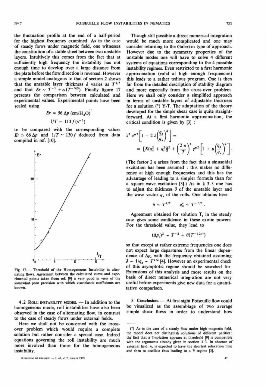
layers. Intuitively this comes from the fact that atsufficiently high frequency the instability has notenough time to develop over a large distance fromthe plate before the flow direction is reversed. Howevera simple model analogous to that of section 2 showsthat the unstable layer thickness b varies as T 2/5and that Er- T -1 + o (T - 3/5). Finally figure 17

presents the comparison between calculated and

experimental values. Experimental points have beenscaled using

to be compared with the corresponding values

Er £r 66 Ap and 1/T ~ 130 f deduced from data

compiled in ref. [10].

Fig. 17. - Threshold of the Homogeneous Instability in alter-

nating flows. Agreement between the calculated curve and expe-rimental points taken from ref. [9] is very good in view of thesomewhat poor precision with which viscoelastic coefficients areknown.

4.2 ROLL INSTABILI1Y MODES. - In addition to the

homogeneous mode, roll instabilities have also beenobserved in the case of alternating flow, in contrastto the case of steady flows under external fields.Here we shall not be concerned with the cross-

over problem which would require a completesolution but rather consider a special case. Indeedequations governing the roll instability are muchmore involved than those for the homogeneousinstability.

Though still possible a direct numerical integrationwould be much more complicated and one mayconsider retuming to the Galerkin type of approach.However due to the symmetry properties of theunstable modes one will have to solve 4 different

systems of equations corresponding to the 4 possibleinstability regimes. Even restricted to a first harmonicapproximation (valid at high enough frequencies)this leads to a rather tedious program. One is thenfar from the detailed description of stability diagramand more especially from the cross-over problem.Here we shall only consider a simplified approachin terms of unstable layers of adjustable thicknessfor a solution (4) Y-T. The adaptation of the theorydeveloped for the simple shear case is quite straight-forward. At a first harmonic approximation, the

critical condition is given by [3] :

(The factor 2 03C0 arises from the fact that a sinusoidalexcitation has been assumed : this makes no diffe-rence at high enough frequencies and this has theadvantage of leading to a simpler formula than fora square wave excitation [3].) As in § 3.3 one hasto adjust the thickness ô of the unstable layer andthe wave vector qx of the rolls. One obtains here

Agreement obtained for solution T, in the steadycase gives some confidence in these exotic powers.For the threshold value, they lead to

so that except at rather extreme frequencies one doesnot expect large departures from the linear depen-dence of L1pc with the frequency obtained assumingS N 1/qx~ T 1/2 [4]. However an experimental checkof this asymptotic regime should be searched for.Extensions of this analysis and more results on thebasis of direct numerical integration are not veryuseful before experiments give new data for a quanti-tative comparison.

5. Conclusion. - At first sight Poiseuille flow couldbe visualized as the assemblage of two averagesimple shear flows in order to understand how

(4) As in the case of a steady flow under high magnetic field,the model does not distinguish solutions of different parities ;the fact that a T-solution appears at threshold [9] is compatiblewith the arguments already given in section 3.3. In absence ofexternal field, ny is expected to have the shortest relaxation timeand then to oscillate thus leading to a Y-regime [3].

724

hydrodynamic instabilities can occur. However to acertain extent the experimental situation turned outto be more complex than what could be expectedfrom the transposition of results obtained in the

simple shear case. This paper has been mainly devotedto the account of that surprising diversity whichoriginates from the spatial dependence of the basicshearing rate s(z) oc z. (i) In agreement with expe-rimental results rolls analogous to those which

develop in the simple shear case have been shownto have a threshold much higher than that of thehomogeneous solution. (ii) In addition we havebeen able to account for the existence of the secondmetastable homogeneous regime with average twistand no transverse flow observed above the thresholdof the first one associated with net transverse flow.

(iii) A modification of the original Pieranski-Guyoninstability mechanism leads to a long wavelengthroll system with average splay. The threshold ofthis instability (which was observed in the firstseries of experiments) strongly depends on theviscoelastic constants and more especially on theratio a3/a2. This sensitivity (quite sufficient to explainthe absence of this solution in the second series of

experiments) immediately suggests the performanceof experiments with a nematic compound where «3is positive and small, a situation which forbids

homogeneous regimes but leaves intact the mechanismfor this particular instability mode.The three points mentioned above required quanti-

tative predictions. Reliable results have been obtainedusing an extension of the Galerkin method developedpreviously. However calculations are rather long,tedious and expensive, moreover they are nearlyuntractable in the case of altemating flows. Thesefacts have urged one to develop approximate models.The important point was to take into account thespatial dependence of the shear in a simplified butrealistic way. Consideration of fluctuation profiles

’obtained by exact calculations has led to the notion

of unstable layer of variable thickness submitted toan average shearing rate, the thickness of the layerbeing determined by some consistency condition.

Comparison with exact results gives some confidencein such approximate models at least as long as theupper and lower halves of the channel are decoupledby a stable sheet, which is pretty well achieved inthe case of average twist rolls. An application has beengiven for the so-called Y-regime in an altemating Poi-seuille flow.

Theoretical analysis of altemating flows is ratherdifficult from a practical point of view even if it isnot so complicated conceptually. Beside the develop-ment of approximate models there is another approachwhich seems worth-while, namely the direct inte-

gration of the partial differential set of equationstaken as an initial and boundary value problem.This method has given excellent results for the

altemating homogeneous instability and one can

perhaps think of it for more complex situations.Of course many points remains to be studied such

as the truly quantitative account of rolls in alter-

nating flow (and more especially the cross-over.

from uniform distortion to rolls, non-linear effectsfor the Z-regime...) and further experiments havebeen suggested which require a check so that ourpaper can by no means be considered as exhaustive.However we think that the kind of approach whichhas been used, combining experimental results withan analysis of mechanisms, detailed calculations,approximate models and numerical simulation canlead to a rather thorough understanding of physicalphenomena which occur in complex systems suchas flowing nematic liquid crystals as described bythe Ericksen-Leslie hydrodynamic theory.

Acknowledgments. - The author would like to

thank E. Dubois-Violette and P. Pieranski for inte-

resting discussion conceming theoretical and expe-rimental aspects of this work.

References

[1] JENKINS, J. T., Annu. Rev. Fluid Mech. 10 (1978) 197.

DUBOIS-VIOLETTE, E. et al., in Liquid Crystals supplement 14to Solid. State Phys., L. Liebert ed. (Academic Press,New York) 1978.

LESLIE, F. M., in Adv. Liq. Cryst. 4 Brown ed. (AcademicPress, New York) to appear.

[2] PIERANSKI, P. and GUYON, E., Solid State Commun. 13 (1973)435, Phys. Rev. A 9 (1974) 404.

[3] DUBOIS-VIOLETTE, E. et al., J. Méc. 16 (1977) 733.LESLIE, F. M., J. Phys. D 9 (1976) 925 and Mol. Cryst. Liq.

Cryst. 37 (1976) 335.[4] GUYON, E. and PIERANSKI, P., J. Physique Colloq. 36 (1975)

C1-203.

[5] MANNEVILLE, P. and DUBOIS-VIOLETTE, E., J. Physique 37(1976) 1115.

[6] MANNEVILLE, P., Ph. D thesis, Univ. Paris-Sud n° 1912 (1977).[7] MANNEVILLE, P. and DUBOIS-VIOLETTE, E., J. Physique 37

(1976) 285

[8] See for example CHANDRASECKHAR, S., Hydrodynamic andHydromagnetic stability (Clarendon Press, Oxford) 1961.

[9] JANOSSY, I., PIERANSKI, P. and GUYON, E., J. Physique 37(1976) 1105.

[10] See for example : DE GENNES, P. G., The Physics of LiquidCrystals (Clarendon Press, Oxford) 1974.

[11] A recent review of alternating flow stability has been given byDAVIS, Annu. Rev. Fluid Mech. 8 (1976) 57.

[12] This is similar to the case of electrohydrodynamic instabilitiesin nematic liquid crystals under alternating electrical fieldssee :

DUBOIS-VIOLETTE, E., DE GENNES, P. G. and PARODI, O.,J. Physique 32 (1971) 305.

[13] RICHTMYER, R. D., MORTON, K. W., Difference Methods forInitial Value Problems (Interscience Publisher-Wiley,New York) 1967.