Physics and Chemistry of the Earth 35 (2010) 11–18

Contents lists available at ScienceDirect

Physics and Chemistry of the Earth

journal homepage: www.elsevier .com/locate /pce

Effect of evapotranspiration parameterisation on the Palmer Drought Severity Index

Szilvia Horváth a,1, István Jankó Szép b, László Makra a, János Mika c,d,*, Ilona Pajtók-Tari d, Zoltán Utasi d

a Department of Climatology and Landscape Ecology, University of Szeged, H-6701 Szeged, P.O.B. 653, Hungaryb PhD School in Geography, Eotvos Lorand University, Budapest, Hungaryc Hungarian Meteorological Service, H-1525 Budapest, P.O.B. 38, Hungaryd Department of Geography, Eszterházy Károly College, H-3300 Eger, Leányka 6, Hungary

a r t i c l e i n f o a b s t r a c t

Article history:Available online 10 March 2010

Keywords:EvapotranspirationBlaney–CriddleThornthwaiteTime and space variability

1474-7065/$ - see front matter � 2010 Elsevier Ltd. Adoi:10.1016/j.pce.2010.03.015

* Corresponding author at: Hungarian MeteorologicP.O. Box 38, Hungary. Tel.: +36 1 346 47 10, mobile:346 46 69.

E-mail addresses: horvathszil@mail.kvvm.hu (S. H(I.J. Szép), makra@geo.u-szeged.hu (L. Makra), mika.jektf.hu (I. Pajtók-Tari), utasiz@ektf.hu (Z. Utasi).

1 Present address: Ministry of Environment and WPolicy and Impact Assessment Department. 1011 Buda

The aim of the study is to compare two popular parameterisations of potential evapotranspiration,applied in computation of the Palmer Drought Severity Index. Among other differences, Thornthwaitemethod considers bare soil, whereas Blaney–Criddle method estimates evapotranspiration after specifi-cation of a given plant. Monthly PDSI series in the April–October growing season of maize are analysed atfive stations in Eastern Hungary for the period 1901–1999. When using Blaney–Criddle method both theinter-annual and inter-monthly variability, i.e. standard deviation and auto-correlation decrease. Trendsand regression coefficients to hemispheric temperature changes are smaller for latter parameterisation,as well. Synchronous correlation among the stations also decreases in this latter approach, whereas nor-mality of the distribution remains valid in majority of months and stations.

� 2010 Elsevier Ltd. All rights reserved.

1. Introduction

The increasing awareness of the effects of drought has led to alarge number of regional and large-scale studies in various climaticregions (Dai et al., 1998, 2004; Wilhite, 2000; Domonkos et al.,2001; Panu and Sharma, 2002; Svoboda et al., 2002; Pongráczet al., 2003; Stefan et al., 2004; van der Schrier et al., 2006, 2007;Blenkinsop and Fowler, 2007; Marsh et al., 2007).

Several drought indices have been used to analyse onset andduration of drought, recently overviewed e.g. by Heim (2002).The Palmer Drought Severity Index (PDSI) is one of the most widelyapplied indices for quantification of droughts all over the world(Szinell et al., 1998; Lloyd-Hughes and Saunders, 2002; Dai et al.,2004; van der Schrier et al., 2007). A comprehensive overview ofthe calculation procedures to derive the PDSI and its monthlyincrement, the Z-index is found in Palmer (1965, 1968), Alley(1984) and van der Schrier et al. (2006, 2007).

The PDSI is such an index of meteorological drought, values ofwhich are calculated from of precipitation and temperature, as wellas water capacity of soil for the actual and preceding periods. PDSI isstandardised for different regions and time periods, which is usefulin common assessment for a wide area with different climate. If

ll rights reserved.

al Service, H-1525 Budapest,+36 70 330 79 50; fax: +36 1

orváth), jankoszi@yahoo.com@met.hu (J. Mika), pajtokil@

ater Hungary, Environmentalpest, F}o u. 44-50, Hungary.

PDSI values are negative (positive), they indicate dry (wet) period,while those around zero denote near-average water balance. Pal-mer considered ±4 as a threshold value of extremity (Palmer, 1965).

Some former studies (Horváth, 2002; Jankó Szép et al., 2005;Mika et al., 2005; Makra et al., 2002, 2005) have already analysedvarious features of PDSI in different sectors of Hungary. These pa-pers reflect several aspects of PDSI and the key international liter-ature sources on the field exhibit a 40-year long history sincePalmer‘s historical paper in 1965.

The study aims at examining if an alternative approach to thepotential evapotranspiration, i.e. the Blaney–Criddle approachmay strongly affect some of the features having been establishedin the above papers. For this purpose, two versions of PDSI arecompared, differing only in estimating the potential evapotranspi-ration. The Thornthwaite (1948) method operates with meteoro-logical variables, irrespectively to the vegetation, i.e. potentialevapotranspiration is estimated as evaporation of bare surface,only. In spite of this, the Blaney–Criddle method (Alley, 1984) usesplant constants to estimate potential evapotranspiration. To spec-ify this methodology, maize is selected as typical for managed veg-etation of the country. The study area is the plain area of the TiszaRiver in Eastern Hungary.

2. The study area and data of analysis

2.1. The study area

Similarly to our former studies dealing with the Palmer Index(Horváth, 2002; Makra et al., 2002, 2005; Mika et al., 2005), the

12 S. Horváth et al. / Physics and Chemistry of the Earth 35 (2010) 11–18

present analysis is also based on monthly PDSI times series of Mis-kolc, Nyíregyháza, Debrecen, Kecskemét and Szeged on the plaincatchment area of the Tisza River in Eastern Hungary (Fig. 1) forthe period 1901–1999. Selection of the region is motivated by itsimportant agricultural activity, by repeated drought and inunda-tion. Natural protection is also crucial, since 70–80% of the areais covered by managed vegetation.

Hereinafter, results of the growing season, i.e. for April–Octoberare analysed. In some cases, every second month (April, June, Au-gust and October) is only presented, considering the strong auto-correlation of the PDSI.

2.2. The Palmer Drought Severity Index

2.2.1. Computation of PDSICalculation of the Index, consisting of five steps, is described in a

few papers (Palmer, 1965; Alley, 1984; Karl, 1986). The procedureconsiders monthly precipitation, temperature and soil water capacityconditions. Basic concepts and steps of computation are as follows:

Step 1: Hydrological Accounting. Computation of PDSI beginswith a climatic water balance using series of monthly precipitationand temperature records. An empirical procedure is used to ac-count for soil water storage by dividing the soil into two arbitrarylayers. The upper layer is assumed to contain 25 mm of availablewater at field capacity. The loss from the underlying layer dependson the initial water content, as well as on the computed potentialevapotranspiration (PET) and the Available Water Capacity (AWC)

BS

Her

nád

Zagyva

Körös

Maros

Sajó

Tisza

Tisz

a

Miskolc

Kecskemét

Szeged

45 km30150

Fig. 1. The study area with the five inv

of the soil system. In the present calculations of PDSI, AWC valuesof 100 mm are used for all stations, even with, possibly, differentsoil types. Runoff is assumed to occur, if and only if, both layersreach their combined water capacity, AWC. In addition to PET, threemore potential terms are used and defined as follows: Potential Re-charge is the amount of water required to bring the soil to its waterholding capacity. Potential Loss is the amount of water that couldbe lost from the soil by evapotranspiration during a zero precipita-tion period. Potential Runoff is defined as the difference betweenprecipitation and Potential Recharge.

Step 2: Climatic Coefficients. This is accomplished by simulatingthe water balance for the period of available weather records.Monthly coefficients are computed as proportions between cli-matic averages of actual vs. potential values of evaporation, re-charge, runoff and loss, respectively.

Step 3: CAFEC Values. The derived coefficients are used to deter-mine the amount of precipitation (I) required for the ClimaticallyAppropriate For Existing Conditions (CAFEC), i.e. ‘‘normal” weatherduring each individual month.

Step 4: Moisture Anomaly Index. Difference between the actualand the CAFEC precipitation is an indicator of water deficiency orsurplus in that month and station, expressed as D = P � I. Thesedepartures are converted into indices of moisture anomaly asZ = K(j)D, where K(j) is a weighting factor for the month j, alsoaccounting for spatial variability of the departures (D).

Step 5: Drought Severity. In the final step the Z-index time seriesare analysed to develop criteria for the beginning and ending of

Kraszna

erett

yó

ebes-Körös

Fekete-

KörösFehér-Körös

Szamos

Bodrog Tisza

Debrecen

Nyíregyháza

estigated stations in East Hungary.

S. Horváth et al. / Physics and Chemistry of the Earth 35 (2010) 11–18 13

drought periods and an empirical formula for determining droughtseverity, such as:

Xj ¼ 0:897Xj�1 þ Zj=3;

where Zj is the Moisture Anomaly Index and Xj is the value of PDSIfor the jth month.

The equation indicates that PDSI of a given month stronglydepends on the conditions of the previous months and on themoisture anomaly of the actual month. This fact implies strongauto-correlation of PDSI.

Monthly time series of temperatures and precipitation, as inputdata of the Index, exhibit inhomogeneity due to changes in obser-vation times, transfer of stations and other possible factors.Homogenisation of the monthly temperature and precipitationdata is performed by the statistical procedure of MASH (MultipleAnalysis for Homogenisation) elaborated in the Hungarian Meteo-rological Service (Szentimrey, 1995, 1999). The essence of the pro-cedure is a break-point analysis assuming that all real changes ofthe local macro-climate occur in a smooth way; hence any signif-icant break-point of the series should be corrected. The MASH pro-cedure and software is used in several other countries, as well(WMO, 2004).

2.2.2. Two methods for estimating potential evapotranspirationCalculation of PDSI may differ in the way of how potential

evapotranspiration is estimated. Palmer used the formula ofThornthwaite in his Index for calculating potential evapotranspira-tion (Thornthwaite, 1948); however, application of the Blaney–Criddle method offered alternative assessment later (Alley, 1984).The first method considers evapotranspiration as a climate vari-able, without specific vegetation, whereas the second approach re-flects some specifics of the vegetation, as well. Thereinafter, thetwo methods of calculating potential evapotranspiration, requiredfor computing PDSI, are briefly specified.

The Blaney–Criddle (B–C in the followings) method belongs tothe group of empirical methods, mainly used in agricultural andwater management calculations. The method estimates the quan-tity of water utilised by vegetation (CU = consumptive water use)which equals to the potential evapotranspiration (PET):

CU ¼ PET ¼ k:c:pð0:46T þ 8Þ ½mm day�1� ð1Þ

where T is daily average temperature (�C); c is a constant, depend-ing of daily minimum of relative humidity, wind speed and relativehumidity; p is a coefficient depending of geographical latitude,which represents average daily ratio of sunshine duration per lati-tude. Value of k, as a plant factor, is location-specific. The expression(0.46T + 8) in Eq. (1) is the average value of PET, which is improvedby c in order to make its value more precise.

When using the B–C method for calculating potential evapo-transpiration, a so called reference plant should be considered.For this aim, the selected reference plant is maize, since it is char-acteristic for the investigated region (Mika et al., 2001), and itsquickly developing leaf surface is also similar to several other agri-cultural plants, from transpiration point of view, as well.

The Thornthwaite (Th in the followings) method is based on theexperience that potential evapotranspiration (PET) is competentlydetermined by temperature. The procedure can be used for calcu-lating PET sums of large regions; however, it does not explicitly re-flect its dependence from air humidity and windiness. Its formula,simplified by Thornthwaite is:

PET ¼ 1:6 � 10 � TI

� �a

ð2Þ

where T is monthly average temperature (�C), while I is the so calledheat index,

I ¼ 125� T1:514; ð3Þ

whereas the exponent a can be calculated as follows:

a ¼ 6:75 � 10�7I3 � 7:71 � 10�5 � I2 þ 1:792 � 10�2 � I þ 4:9239 � 10�1

ð4Þ

The two methods for calculating potential evapotranspira-tion can modify our results published in former studies,although we received strong significant correlation (0.86 <r < 0.98) between monthly PDSI data sets calculated with Thand B–C methods (Mika et al., 2005). In this paper PDSI seriesconsidering: (a) B–C method; and (b) Th method are comparedfor the period 1901–1999 at the above five stations. Eightfurther aspects (see titles of Section 4) are presented to charac-terise the differences in PDSI caused only by the evapotran-spiration method.

At the end of description of the key process of our paper, i.e. thePDSI computation, we must admire that all our computations usethe traditional way of PDSI where the constants of the processare used, as it had been set by Palmer (1965). Since then, the so-called self-calibrated PDSI (scPDSI) has been defined in the litera-ture which improved the ‘traditional’ PDSI (Wells et al., 2004). Thisimprovement means that the empirical weighting factors, de-scribed above, are individually set according to climate of the givenstation. However, these parameter-settings are performed to pro-vide long-term balances which also depend on the applied evapo-transpiration methodology. This ‘‘self-calibration” of the PDSIwould also obscure the effects of the evapotranspiration processes,as well.

2.3. Further data

2.3.1. Soil moisture estimationThe calculated PDSI values were compared to the soil moisture

content (SMC) of the upper 1 m soil layer, quantified for a shorterperiod, 1901–1990, in an independent way (Dunkel, 1994; JankóSzép et al., 2005). The latter data were available for three stationsof the region: Nyíregyháza, Debrecen and Szeged. Computation ofSMC also considers daily changes of the water balance, but it para-meterises evapotranspiration (both the potential and the real ones)in a different way. The original source of data (Dunkel, 1994) alsocontains some verification against the data of a direct soil moisturemeasuring network.

2.3.2. Hemispherical mean temperatureComparison of PDSI with the global climate tendency re-

quests data on mean temperature (<T>) of the Northern hemi-sphere and those for air temperature contrast betweencontinents and oceans (DT). They are derived from air tempera-ture data over the continents (Jones, 1994 and updated) andover the oceans (Folland et al., 1984 and updated), consideringthe proportionality of the two surface-types. The original up-dated time series are available from internet: http://cdiac.esd.ornl.gov/trends/temp/jonescru/jones.html. Since air tempera-ture data sets over the oceans are available till 1988 (Follandet al., 1984 and updated), DT for the 1989–1999 period betweenis estimated from regression with <T>. This estimation indicatessignificant connection only in monotonously warming (or cool-ing) periods. Data of the last 11 years were estimated from thenorthern hemispheric mean temperature using the clearlywarming periods of 1917–1943 and 1976–1988, i.e. altogether40 years (Jones et al., 2000).

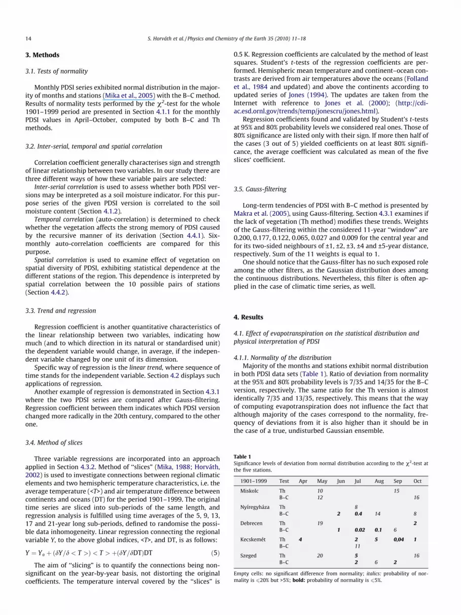
Table 1Significance levels of deviation from normal distribution according to the v2-test atthe five stations.

1901–1999 Test Apr May Jun Jul Aug Sep Oct

Miskolc Th 10 15B–C 12 16

Nyíregyháza Th 8B–C 2 0.4 14 8

Debrecen Th 19 2B–C 1 0.02 0.1 6

Kecskemét Th 4 2 5 0,04 1B–C 11

Szeged Th 20 5 16B–C 2 6 2

Empty cells: no significant difference from normality; italics: probability of nor-mality is 620% but >5%; bold: probability of normality is 65%.

14 S. Horváth et al. / Physics and Chemistry of the Earth 35 (2010) 11–18

3. Methods

3.1. Tests of normality

Monthly PDSI series exhibited normal distribution in the major-ity of months and stations (Mika et al., 2005) with the B–C method.Results of normality tests performed by the v2-test for the whole1901–1999 period are presented in Section 4.1.1 for the monthlyPDSI values in April–October, computed by both B–C and Thmethods.

3.2. Inter-serial, temporal and spatial correlation

Correlation coefficient generally characterises sign and strengthof linear relationship between two variables. In our study there arethree different ways of how these variable pairs are selected:

Inter-serial correlation is used to assess whether both PDSI ver-sions may be interpreted as a soil moisture indicator. For this pur-pose series of the given PDSI version is correlated to the soilmoisture content (Section 4.1.2).

Temporal correlation (auto-correlation) is determined to checkwhether the vegetation affects the strong memory of PDSI causedby the recursive manner of its derivation (Section 4.4.1). Six-monthly auto-correlation coefficients are compared for thispurpose.

Spatial correlation is used to examine effect of vegetation onspatial diversity of PDSI, exhibiting statistical dependence at thedifferent stations of the region. This dependence is interpreted byspatial correlation between the 10 possible pairs of stations(Section 4.4.2).

3.3. Trend and regression

Regression coefficient is another quantitative characteristics ofthe linear relationship between two variables, indicating howmuch (and to which direction in its natural or standardised unit)the dependent variable would change, in average, if the indepen-dent variable changed by one unit of its dimension.

Specific way of regression is the linear trend, where sequence oftime stands for the independent variable. Section 4.2 displays suchapplications of regression.

Another example of regression is demonstrated in Section 4.3.1where the two PDSI series are compared after Gauss-filtering.Regression coefficient between them indicates which PDSI versionchanged more radically in the 20th century, compared to the otherone.

3.4. Method of slices

Three variable regressions are incorporated into an approachapplied in Section 4.3.2. Method of ‘‘slices” (Mika, 1988; Horváth,2002) is used to investigate connections between regional climaticelements and two hemispheric temperature characteristics, i.e. theaverage temperature (<T>) and air temperature difference betweencontinents and oceans (DT) for the period 1901–1999. The originaltime series are sliced into sub-periods of the same length, andregression analysis is fulfilled using time averages of the 5, 9, 13,17 and 21-year long sub-periods, defined to randomise the possi-ble data inhomogeneity. Linear regression connecting the regionalvariable Y, to the above global indices, <T>, and DT, is as follows:

Y ¼ Yo þ ðdY=d < T >Þ < T > þðdY=dDTÞDT ð5Þ

The aim of ‘‘slicing” is to quantify the connections being non-significant on the year-by-year basis, not distorting the originalcoefficients. The temperature interval covered by the ‘‘slices” is

0.5 K. Regression coefficients are calculated by the method of leastsquares. Student’s t-tests of the regression coefficients are per-formed. Hemispheric mean temperature and continent–ocean con-trasts are derived from air temperatures above the oceans (Follandet al., 1984 and updated) and above the continents according toupdated series of Jones (1994). The updates are taken from theInternet with reference to Jones et al. (2000); (http://cdi-ac.esd.ornl.gov/trends/temp/jonescru/jones.html).

Regression coefficients found and validated by Student’s t-testsat 95% and 80% probability levels we considered real ones. Those of80% significance are listed only with their sign. If more then half ofthe cases (3 out of 5) yielded coefficients on at least 80% signifi-cance, the average coefficient was calculated as mean of the fiveslices‘ coefficient.

3.5. Gauss-filtering

Long-term tendencies of PDSI with B–C method is presented byMakra et al. (2005), using Gauss-filtering. Section 4.3.1 examines ifthe lack of vegetation (Th method) modifies these trends. Weightsof the Gauss-filtering within the considered 11-year ‘‘window” are0.200, 0.177, 0.122, 0.065, 0.027 and 0.009 for the central year andfor its two-sided neighbours of ±1, ±2, ±3, ±4 and ±5-year distance,respectively. Sum of the 11 weights is equal to 1.

One should notice that the Gauss-filter has no such exposed roleamong the other filters, as the Gaussian distribution does amongthe continuous distributions. Nevertheless, this filter is often ap-plied in the case of climatic time series, as well.

4. Results

4.1. Effect of evapotranspiration on the statistical distribution andphysical interpretation of PDSI

4.1.1. Normality of the distributionMajority of the months and stations exhibit normal distribution

in both PDSI data sets (Table 1). Ratio of deviation from normalityat the 95% and 80% probability levels is 7/35 and 14/35 for the B–Cversion, respectively. The same ratio for the Th version is almostidentically 7/35 and 13/35, respectively. This means that the wayof computing evapotranspiration does not influence the fact thatalthough majority of the cases correspond to the normality, fre-quency of deviations from it is also higher than it should be inthe case of a true, undisturbed Gaussian ensemble.

S. Horváth et al. / Physics and Chemistry of the Earth 35 (2010) 11–18 15

4.1.2. Correlation with the soil moisture contentPDSI series computed by the B–C version exhibited close rela-

tion with the independent series of monthly soil moisture content,SMC (Mika et al., 2005). On the basis of linear regression coeffi-cients the index values could also be expressed in physical unitsof water content in the upper 1 m soil layer.

With except of the May–June peak of precipitation, correlationcoefficients are somewhat higher for the B–C method than forthe Th method. The most common feature of both PDSI series isthat they exhibit strong correlation with the SMC in all 7 months,analysed (April–October). Although SMC is an independent estima-tion of soil moisture, the correlation between SMC and PDSI may asstrongly influenced by the given methodology of the soil moistureestimation, as by the way of computing evapotranspiration in thePDSI. Therefore, the above relation surely does not mean that B–C is better than Th in this respect.

For the standardised regression coefficients between PDSI val-ues, calculated with the B–C method and moisture content, it canbe established that they are very similar in each of the 7 monthand three stations (Nyíregyháza, Debrecen, Szeged) (Table 2). Unitchange of PDSI calculated with the Th method is connected to theSMC series with slightly lower standardised regressions than thosecalculated with the B–C method.

4.2. Effects of evapotranspiration on the short-term variability of PDSI

4.2.1. Linear trendsLinear trends of the two PDSI versions are presented in Table 3

for every second month of the growing season from April to Octo-ber. Proportion of significant trends is not too high, according tothe t-test at the 95% probability level, but the uniformly negativetendency is worth for attention. This means, that soil of the exam-ined region was characterised with slow drying out in the 20thcentury.

Comparing absolute values of the trends, obtained by the Thand B–C methods in the given 99-year long time sequence, one

Table 2Dimensionless regression coefficients (Ky/ry) between Dunkel‘s soil moisturecontent (SMC), standardised by its standard deviation, and the given PDSI versions(B–C or Th), 1901–1990. Unit change in B–C mean slightly stronger change in thestandardised SMC.

SMCstand/PDSI April May June July August September October

NyíregyházaB–C 0.33 0.35 0.39 0.39 0.37 0.36 0.38Th 0.32 0.35 0.36 0.37 0.34 0.32 0.33

DebrecenBC homog 0.31 0.31 0.37 0.39 0.35 0.36 0.35Th homog 0.30 0.31 0.35 0.36 0.33 0.31 0.31

SzegedBC homog 0.30 0.34 0.37 0.37 0.33 0.34 0.35Th homog 0.28 0.31 0.33 0.33 0.29 0.28 0.30

Table 3Linear trends of PDSI (1/100 years) in both Th and B–C versions for 1901–1999.Significant trends at 5%, according to the t-test, are bold set (Contribution of thetrends to the variance is shown in Fig. 2.).

Station April June August October

Th B–C Th B–C Th B–C Th B–C

Miskolc �2.1 �2.1 �1.3 �1.5 �1.4 �1.5 �2.0 �1.9Nyíregyháza �2.3 �1.6 �1.2 �0.7 �1.4 �1.2 �2.2 �1.8Debrecen �1.7 �1.6 �0.6 �0.7 �0.5 �0.7 �1.5 �1.7Kecskemét �3.3 �2.5 �2.0 �1.2 �2.2 �17 �3.7 �2.2Szeged �3.3 �3.1 �2.5 �1.7 �1.7 �0.9 �2.4 �2.0

can find that the previous one is generally stronger. From amongthe 20 pairs (i.e. five stations and 4 months) there are only5 months, at two stations, where PDSI with B–C evapotranspirationestimation show steeper linear decrease than the same values forthe Th evaporation estimation. This means that the previous ap-proach confined the drying tendency during the 20th century tosome extent.

4.2.2. Variance of original and de-trended seriesComparison of variances (i.e. squares of the standard deviation)

between the two methods is demonstrated in Fig. 2. Height of thecolumns indicates the total variance, whereas smaller white partsat their bottom part show the contribution of the above lineartrends on the variance. The larger part of the columns can be inter-preted as inter-annual variability of PDSI.

Monthly variance of PDSI with the Th method is higher in eachstation than those with the B–C method. Although, the individualdifferences are generally not significant according to the F-test,the B–C approach could slightly decrease the inter-annual variabil-ity of PDSI.

4.3. Effects of evapotranspiration on long-term variability of PDSI

4.3.1. Time-evolution of Gauss-filtered series in the 20th centuryLinear trends are just rough first approximations of the ten-

dency. Results of Gauss-filtering, with the same 11-year windowas specified above in Section 3.5, are presented by Makra et al.(2005) for the B–C version. Here we give a quantitative comparisonof the smoothed Th and B–C series by their regression coefficients(Fig. 3).

In majority of the stations and months the regression coefficientis higher than 1.0. This means that smoothed changes of the Thversion are generally steeper than those for the B–C version. Theonly exception is Miskolc characterised by its most northern posi-tion within the region, surrounded by hills in 3 months from thefour indicated.

In some cases the coefficient is higher than 1.2, indicating thatlack of vegetation would add more than 20% to the drying tendencyof the 20th century in theses months and locations.

0.0

1.0

2.0

3.0

4.0

5.0

6.0

7.0

8.0linear trend variability

M Ny M Ny D K Sz

April June

August October

M M Ny D K Sz SzKD Sz KNy D

Fig. 2. Variance of monthly PDSI values in the five stations (M – Miskolc, Ny –Nyíregyháza, D – Debrecen, K – Kecskemét, Sz – Szeged) as a sum of contributionfrom the linear trends (see in Table 3) and the inter-annual variability. Left columnof each pair is the Thorthwaite version, right side is the Blaney–Criddle version. Thelatter variance is always smaller, mainly due to the inter-annual differences. Role oflinear trends is rather small in the total variance.

0.7

0.8

0.9

1.0

1.1

1.2

1.3

1.4

1.5

April

b

Miskolc Nyíregyháza Debrecen Kecskemét Szeged

June August October

Fig. 3. Regression coefficients between Gauss-filtered PDSI series with 11 yearswindow in the two different versions, in 1906–1994. In the given consideration Thversion is the dependent variable, and B–C version is the independent variable.Regression >1.0 mean stronger changes in Th version than in the B–C during theinvestigated period.

16 S. Horváth et al. / Physics and Chemistry of the Earth 35 (2010) 11–18

4.3.2. Correlation to hemispheric mean temperatureThe drying tendency, demonstrated in the previous sections can

be understood only if comparing to the global climate processes,instead of simple sequence of time, only. (This does not mean,however, that water balance could not be influenced by those localinterventions that are just casual functions of time. Such effects,nevertheless, are not involved into the PDSI process operating,e.g. with the same water holding capacity, or soil layer thickness.)Comparison of local PDSI to hemispheric mean temperature, <T>,and continent–ocean contrast, DT, is numerically performed bythe method of slices (Section 3.4).

The detailed results for the B–C version of PDSI are displayed byHorváth (2002). Here we focus on comparison of the two versions,without presenting parallel details concerning the Th version. Keyfigures of this comparison are presented in Table 4, in which num-ber of all significant partial regression coefficients (4 months at fivestations) between the corresponding PDSI values and the hemi-spheric parameters are displayed together with the averages ofall regression coefficients (R/5: together for the significant andnon-significant ones).

Similarly to the results with the B–C method, significant nega-tive regression coefficients (PDSI/T) dominate the partial relationbetween the PDSI with Th method and the hemispheric mean tem-perature. The average coefficient is also strongly negative. Thismeans drying tendency parallel to the warming of the 20th cen-tury, including long-term fluctuations of the latter series, as well.Comparing the two versions, one may establish that the negativetendencies are slightly more dominant in the case of the Th version(bare soil) considering the proportion of the significant signs andthe average coefficients, as well.

Sign of the significant coefficients regarding the continent–ocean air temperature contrast (PDSI/DT) is balance between posi-tive and negative effects, whereas the mean coefficient (includingagain the non-significant ones, as well) are negative in both the

Table 4Relative sensitivity of the PDSI data sets calculated with the B–C and the Th methods,temperature contrast (DT). April, June, August and October months are considered. Numbmeans, e.g. 8 + 53 = 61% of significance for PDSI/T in the B–C version.

Station month Relative sensitivity 1/K Blaney–Criddle

asign. + sign

Five stations, A–J–A–O months PDSI/T 8PDSI/DT 18

a Sign. = significant at least at the 80% level.b R/5: Average of all (significant and non-significant) coefficients of PDSI/T and PDSI/

Th and B–C versions. Here the average coefficients differ morecharacteristically, but it would not be easy to interpret without de-tailed physical interpretation.

Putting together the overall proportionality of significant coeffi-cients, one may establish slightly more significance in case of theB–C version. While Th exhibits 5 + 51 = 56 significant coefficientsfor PDSI/T and 17 + 14 = 31 ones for PDSI/DT, the version with theB–C approach is characterised by 8 + 53 = 61 and 18 + 21 = 39 sig-nificant coefficients, respectively. Maybe this is also connected tothe fact of the smaller inter-annual variability in the latter case,which, in turn, opens wider space to the statistical governance ofglobal climate tendencies. However, the more frequent significantcoefficients themselves do not mean stronger sensitivity of PDSI inthe case of B–C computation of evapotranspiration, since the aver-age negative PDSI/T coefficients is stronger for the Th version by ca.15% (�2.28 K�1 vs. �1.92 K�1).

4.4. Effects of evapotranspiration on the temporal and spatialcorrelation of PDSI

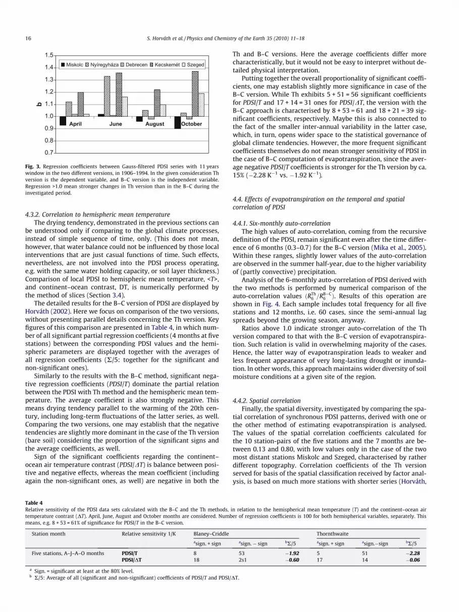
4.4.1. Six-monthly auto-correlationThe high values of auto-correlation, coming from the recursive

definition of the PDSI, remain significant even after the time differ-ence of 6 months (0.3–0.7) for the B–C version (Mika et al., 2005).Within these ranges, slightly lower values of the auto-correlationare observed in the summer half-year, due to the higher variabilityof (partly convective) precipitation.

Analysis of the 6-monthly auto-correlation of PDSI derived withthe two methods is performed by numerical comparison of theauto-correlation values ðRTh

6 =RB—C6 Þ. Results of this operation are

shown in Fig. 4. Each sample includes total frequency for all fivestations and 12 months, i.e. 60 cases, since the semi-annual lagspreads beyond the growing season, anyway.

Ratios above 1.0 indicate stronger auto-correlation of the Thversion compared to that with the B–C version of evapotranspira-tion. Such relation is valid in overwhelming majority of the cases.Hence, the latter way of evapotranspiration leads to weaker andless frequent appearance of very long-lasting drought or inunda-tion. In other words, this approach maintains wider diversity of soilmoisture conditions at a given site of the region.

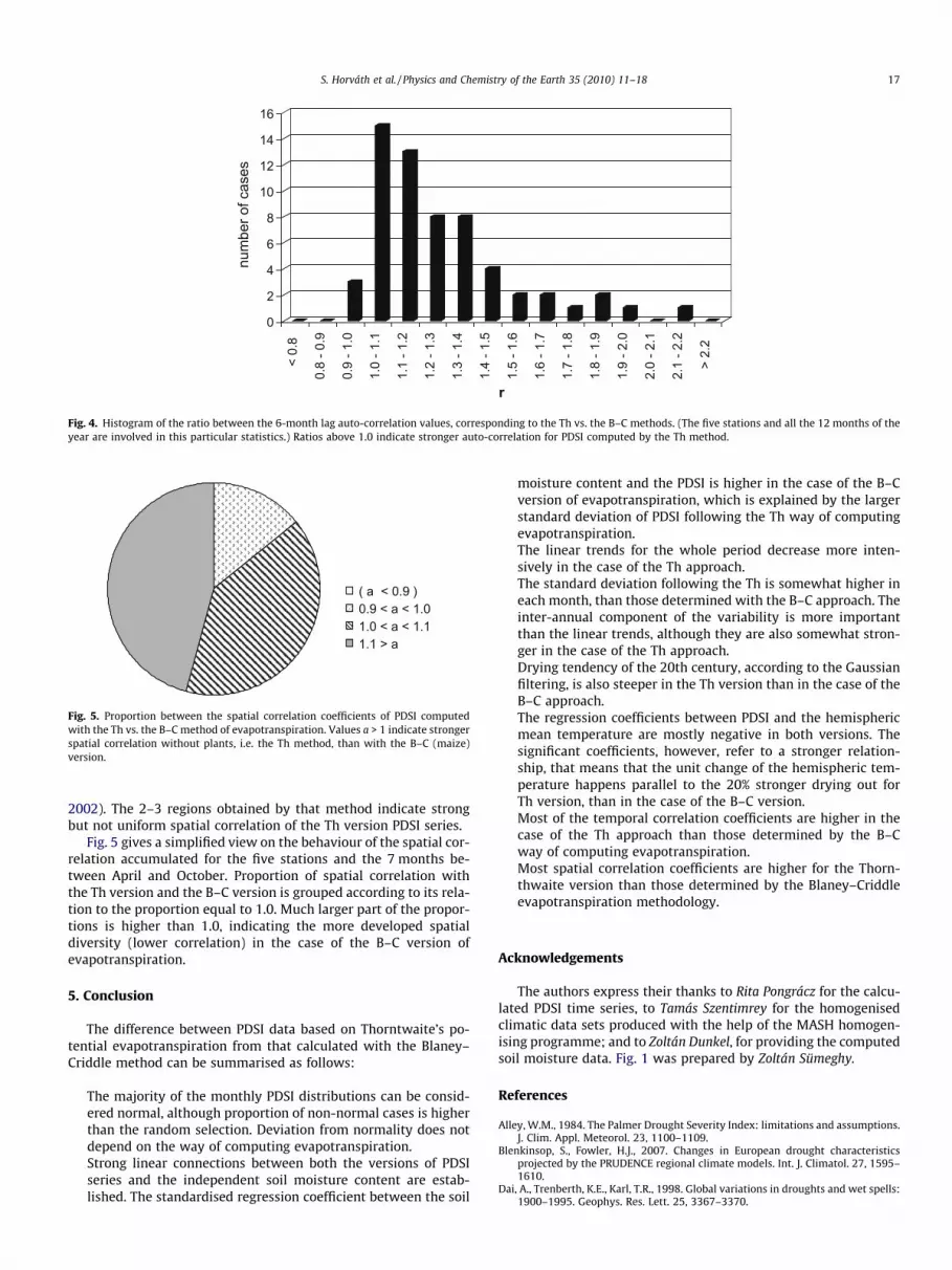
4.4.2. Spatial correlationFinally, the spatial diversity, investigated by comparing the spa-

tial correlation of synchronous PDSI patterns, derived with one orthe other method of estimating evapotranspiration is analysed.The values of the spatial correlation coefficients calculated forthe 10 station-pairs of the five stations and the 7 months are be-tween 0.13 and 0.80, with low values only in the case of the twomost distant stations Miskolc and Szeged, characterised by ratherdifferent topography. Correlation coefficients of the Th versionserved for basis of the spatial classification received by factor anal-ysis, is based on much more stations with shorter series (Horváth,

in relation to the hemispherical mean temperature (T) and the continent–ocean airer of regression coefficients is 100 for both hemispherical variables, separately. This

Thornthwaite

asign. � sign bR/5 asign. + sign asign.�sign bR/5

53 �1.92 5 51 �2.282s1 �0.60 17 14 �0.06

DT.

0

2

4

6

8

10

12

14

16

num

ber o

f cas

es

< 0.

8

0.8

- 0.9

0.9

- 1.0

1.0

- 1.1

1.1

- 1.2

1.2

- 1.3

1.3

- 1.4

1.4

- 1.5

1.5

- 1.6

1.6

- 1.7

1.7

- 1.8

1.8

- 1.9

1.9

- 2.0

2.0

- 2.1

2.1

- 2.2

> 2.

2

r

Fig. 4. Histogram of the ratio between the 6-month lag auto-correlation values, corresponding to the Th vs. the B–C methods. (The five stations and all the 12 months of theyear are involved in this particular statistics.) Ratios above 1.0 indicate stronger auto-correlation for PDSI computed by the Th method.

( a < 0.9 )0.9 < a < 1.01.0 < a < 1.11.1 > a

Fig. 5. Proportion between the spatial correlation coefficients of PDSI computedwith the Th vs. the B–C method of evapotranspiration. Values a > 1 indicate strongerspatial correlation without plants, i.e. the Th method, than with the B–C (maize)version.

S. Horváth et al. / Physics and Chemistry of the Earth 35 (2010) 11–18 17

2002). The 2–3 regions obtained by that method indicate strongbut not uniform spatial correlation of the Th version PDSI series.

Fig. 5 gives a simplified view on the behaviour of the spatial cor-relation accumulated for the five stations and the 7 months be-tween April and October. Proportion of spatial correlation withthe Th version and the B–C version is grouped according to its rela-tion to the proportion equal to 1.0. Much larger part of the propor-tions is higher than 1.0, indicating the more developed spatialdiversity (lower correlation) in the case of the B–C version ofevapotranspiration.

5. Conclusion

The difference between PDSI data based on Thorntwaite’s po-tential evapotranspiration from that calculated with the Blaney–Criddle method can be summarised as follows:

The majority of the monthly PDSI distributions can be consid-ered normal, although proportion of non-normal cases is higherthan the random selection. Deviation from normality does notdepend on the way of computing evapotranspiration.Strong linear connections between both the versions of PDSIseries and the independent soil moisture content are estab-lished. The standardised regression coefficient between the soil

moisture content and the PDSI is higher in the case of the B–Cversion of evapotranspiration, which is explained by the largerstandard deviation of PDSI following the Th way of computingevapotranspiration.The linear trends for the whole period decrease more inten-sively in the case of the Th approach.The standard deviation following the Th is somewhat higher ineach month, than those determined with the B–C approach. Theinter-annual component of the variability is more importantthan the linear trends, although they are also somewhat stron-ger in the case of the Th approach.Drying tendency of the 20th century, according to the Gaussianfiltering, is also steeper in the Th version than in the case of theB–C approach.The regression coefficients between PDSI and the hemisphericmean temperature are mostly negative in both versions. Thesignificant coefficients, however, refer to a stronger relation-ship, that means that the unit change of the hemispheric tem-perature happens parallel to the 20% stronger drying out forTh version, than in the case of the B–C version.Most of the temporal correlation coefficients are higher in thecase of the Th approach than those determined by the B–Cway of computing evapotranspiration.Most spatial correlation coefficients are higher for the Thorn-thwaite version than those determined by the Blaney–Criddleevapotranspiration methodology.

Acknowledgements

The authors express their thanks to Rita Pongrácz for the calcu-lated PDSI time series, to Tamás Szentimrey for the homogenisedclimatic data sets produced with the help of the MASH homogen-ising programme; and to Zoltán Dunkel, for providing the computedsoil moisture data. Fig. 1 was prepared by Zoltán Sümeghy.

References

Alley, W.M., 1984. The Palmer Drought Severity Index: limitations and assumptions.J. Clim. Appl. Meteorol. 23, 1100–1109.

Blenkinsop, S., Fowler, H.J., 2007. Changes in European drought characteristicsprojected by the PRUDENCE regional climate models. Int. J. Climatol. 27, 1595–1610.

Dai, A., Trenberth, K.E., Karl, T.R., 1998. Global variations in droughts and wet spells:1900–1995. Geophys. Res. Lett. 25, 3367–3370.

18 S. Horváth et al. / Physics and Chemistry of the Earth 35 (2010) 11–18

Dai, A., Trenberth, K.E., Qian, T., 2004. A global data set of Palmer Drought SeverityIndex for 1870–2002: relationship with soil moisture and effects of surfacewarming. J. Hydrometeorol. 5, 1117–1130.

Domonkos, P., Szalai, S., Zoboki, J., 2001. Analysis of drought severity using PDSI andSPI indices. Id}ojárás 105, 93–107.

Dunkel, Z., 1994. Investigation of climatic variability influence on soil moisture inHungary. In: XVIIth Conference of the Danube Countries, Budapest, Hungary,pp. 441–446.

Folland, C.K., Parker, D.E., Kates, F.E., 1984. World-wide marine temperaturefluctuations 1856–1981. Nature 310, 670–673.

Heim, R.R., 2002. A review of twentieth-century drought indices used in the UnitedStates. Bull. Am. Meteorol. Soc. 83, 1149–1165.

Horváth, S., 2002. Spatial and temporal patterns of soil moisture variationsin a sub-catchment of River Tisza. Phys. Chem. Earth Part B 27,1051–1062.

Jankó Szép, I., Mika, J., Dunkel, Z., 2005. Palmer Drought Severity Index as soilmoisture indicator: physical interpretation, statistical behaviour and relation toglobal climate. Phys. Chem. Earth 30, 231–244.

Jones, P.D., 1994. Hemispheric surface air temperature variations: a reanalysis, anupdate to. J. Climate 7, 1794–1802.

Jones, P.D., Parker, D.E., Osborn, T.J., Briffa, K.R., 2000. Global and hemispherictemperature anomalies – land and marine instrumental records. In: Trends: ACompendium of Data on Global Change. Carbon Dioxide Information AnalysisCenter, Oak Ridge National Laboratory, US Department of Energy, Oak Ridge,Tennessee, USA.

Karl, T.R., 1986. The sensitivity of the Palmer Drought Severity Index and Palmer’s Zindex to their calibration coefficients including potential evapotranspiration. J.Clim. Appl. Meteorol. 25, 77–86.

Lloyd-Hughes, B., Saunders, M.A., 2002. A drought climatology for Europe. Int. J.Climatol. 22, 1571–1592.

Makra, L., Horváth, S., Pongrácz, R., Mika, J., 2002. Long term climate deviations: analternative approach and application on the Palmer Drought Severity Index inHungary. Phys. Chem. Earth Part B 27, 1063–1071.

Makra, L., Mika, J., Horváth, S., 2005. 20th century variations of the soil moisturecontent in East-Hungary in connection with global warming. Phys. Chem. Earth30, 181–186.

Marsh, T., Cole, G., Wilby, R., 2007. Major droughts in England and Wales, 1800–2006. Weather 62, 87–93.

Mika, J., 1988. Regional characteristics of the global warming in the CarpathianBasin. Id}ojárás 92, 178–189 (in Hungarian).

Mika, J., Horváth, S., Makra, L., 2001. Impact of documented land use changes on thesurface albedo and evapotranspiration in a plain watershed. Phys. Chem. EarthPart B 26, 601–605.

Mika, J., Horváth, S., Makra, L., 2005. The Palmer Drought Severity Index (PDSI) as anindicator of soil moisture. Phys. Chem. Earth 30, 223–230.

Palmer, W.C., 1965. Meteorological Drought. Research Paper, 45, US WeatherBureau, Washington, DC, 58 p.

Palmer, W.C., 1968. Keeping track of crop moisture conditions, nationwide: the cropmoisture index. Weatherwise 21, 156–161.

Panu, U.S., Sharma, T.C., 2002. Challenges in drought research: some perspectivesand future directions. Hydrol. Sci. J. 47 (S), S19–S30.

Pongrácz, R., Bogardi, I., Duckstein, L., 2003. Climatic forcing of droughts: a CentralEuropean example. Hydrol. Sci. J. 48, 39–50.

Stefan, S., Ghioca, M., Rimbu, N., Boroneant, C., 2004. Study of meteorological andhydrological drought in southern Romania from observational data. Int. J.Climatol. 24, 871–881.

Svoboda, M., LeComte, D., Hayes, M., Heim, R., Gleason, K., Angel, J., Rippey, B.,Tinker, R., Palecki, M., Stooksbury, D., Miskus, D., Stephens, S., 2002. The droughtmonitor. Bull. Am. Meteorol. Soc. 83, 1181–1190.

Szentimrey, T., 1995. General problems of the estimations of inhomogeneities,optimal weighting of the reference stations. In: Proceedings of the 6thInternational Meeting on Statistical Climatology. Galway, Ireland, pp. 629–631.

Szentimrey, T., 1999. Multiple analysis of series for homogenization (MASH). In:Proceedings of the Second Seminar for Homogenization of SurfaceClimatological Data, Budapest, Hungary. WMO, WCDMP, vol. 41, pp. 27–46.

Szinell, C., Bussay, A., Szentimrey, T., 1998. Drought tendencies in Hungary. Int. J.Climatol. 18, 1479–1491.

Thornthwaite, C.W., 1948. An approach towards a rational classification of climate.Geogr. Rev. 38, 55–94.

Van der Schrier, G., Briffa, K.R., Jones, P.D., Osborn, T.J., 2006. Summer moisturevariability across Europe. J. Clim. 19, 2818–2834.

van der Schrier, G., Efthymiadis, D., Briffa, K.R., Jones, P.D., 2007. European alpinemoisture variability 1800–2003. Int. J. Climatol. 27, 415–427.

Wells, N., Goddard, S., Hayes, M., 2004. A self-calibrating Palmer Drought SeverityIndex. J. Clim. 17, 2335–2351.

Wilhite, D. (Ed.), 2000. Drought: A Global Assessment, 1. Routledge Publishers,London, p. 422.

WMO. 2004. In: Proceedings of the Fourth Seminar for Homogenization and QualityControl in Climatological Databases, Budapest, Hungary, 6–10 October 2003,WCDMP-No. 56, WMO, Geneva, 243 p.