arX

iv:c

ond-

mat

/061

0630

v2 [

cond

-mat

.mes

-hal

l] 9

Jan

200

7

Dynamical polarization of graphene at finite doping

B. Wunsch1,2, T. Stauber2, F. Sols1, and F. Guinea2

1 Departamento de Fısica de Materiales, Facultad de Ciencias Fısicas,

Universidad Complutense de Madrid, E-28040 Madrid, Spain.

2 Instituto de Ciencia de Materiales de Madrid,

CSIC, Cantoblanco, E-28049 Madrid, Spain.

(Dated: February 6, 2008)

Abstract

The polarization of graphene is calculated exactly within the random phase approximation for

arbitrary frequency, wave vector, and doping. At finite doping, the static susceptibility saturates to

a constant value for low momenta. At q = 2kF it has a discontinuity only in the second derivative.

In the presence of a charged impurity this results in Friedel oscillations which decay with the same

power law as the Thomas Fermi contribution, the latter being always dominant. The spin density

oscillations in the presence of a magnetic impurity are also calculated. The dynamical polarization

for low q and arbitrary ω is employed to calculate the dispersion relation and the decay rate of

plasmons and acoustic phonons as a function of doping. The low screening of graphene, combined

with the absence of a gap, leads to a significant stiffening of the longitudinal acoustic lattice

vibrations.

PACS numbers: 63.20.-e, 73.20.Mf, 73.21.-b

1

I. INTRODUCTION

Recent progress in the isolation of single graphene layers has permitted the realization of

transport and Raman experiments1 which have stimulated an intense theoretical research

on the properties of a monoatomic graphene sheet. Most of the unusual electronic proper-

ties can be understood in terms of a simple tight-binding approach for the π-electrons of

carbon, which yields a gapless linear band structure with a vanishing density of states at

zero doping.2,3

The electronic band structure of an undoped single graphene sheet allows for a descrip-

tion of the electronic properties in terms of an effective field theory which is equivalent to

Quantum Electrodynamics (QED) in 2+1 dimensions. Within such a framework important

physical quantities such as the electron self-energy or the charge and spin susceptibilities

can be calculated exploiting the special symmetries of the model.4

Finite doping away from half-filling qualitatively changes the above description, since

it breaks electron-hole symmetry and also the pseudo Lorentz invariance needed for the

equivalence with QED in two space dimensions. One is thus forced to retreat to conventional

condensed-matter techniques such as e.g. Matsubara Green’s functions. This was recently

done for the static susceptibility of graphene at finite doping5. Similar calculations for bulk

graphite had been performed by Shung et al.,6 who investigated the dielectric function and

the plasmon behavior. Studies of static screening in graphene based on the Thomas-Fermi

approximation had also been considered.7,8 The relation between the polarization and the

transport properties of graphene has been recently discussed in Refs. 5,9,10. Thermo-plasma

polaritons in graphene are discussed in citeVafek.

In this paper, we calculate the dynamical polarization within the random phase approx-

imation (RPA) for arbitrary wavevector, frequency, and doping. We discuss the method of

calculation in the next section. We present in Section III results for static screening, where

we analyze the Friedel oscillations induced by a charged or magnetic impurity, comparing

our results with those of the two-dimensional electron gas (2DEG). Section IV discusses the

plasmon dispersion relation and lifetime. In Section V we analyze the screening of the lon-

gitudinal acoustic modes by the conduction electrons. Finally, Section VI presents the main

conclusions of our work. Some of the more technical aspects of the formalism are explained

in the Appendix.

2

II. RPA CALCULATION

Within the effective mass approximation, and focusing on one of the two unequal K-

points, the Hamiltonian of an hexagonal graphene sheet is given in the Bloch spinor repre-

sentation as2

H = hvF

∑

k

Hk , Hk = ψ†k

−kF φk

φ∗k −kF

ψk . (1)

Here φk = kx + iky and ψk = (ak, bk)T , where ak and bk are the destruction operators

of the Bloch states of the two triangular sublattices. We have also introduced the Fermi

wavevector kF which is related to the chemical potential µ via kF = µ/hvF . The Fermi

velocity vF = 3at/2h is determined by the carbon-carbon distance a = 1.42 A and the

nearest neighbor hopping energy t = 2.7 eV resulting in vF ≃ 9 × 105 m/s.11 We note that

the effective Hamiltonian given above is valid only for wave vectors k ≪ Λ, where Λ ≃ 8.25

eV is a high-energy cutoff stemming from the discreteness of the lattice.11

The quantity of interest for many physical properties is the dynamical polarization, since

it determines e.g. the effective electron-electron interaction, the Friedel oscillations and the

plasmon and phonon spectra. In terms of the bosonic Matsubara frequencies ωn = 2πn/β,

it is defined as12

P (q, iωn) = − 1

A

∫ β

0

dτeiωnτ 〈Tρ(q, τ)ρ(−q, 0)〉 , (2)

where A denotes the area. The average is taken over the canonical ensemble and the density

operator is given by the sum of the density operators of the two sub-lattices ρ = ρa + ρb.

This amounts to working in the long-wavelength limit. To first order in the electron-electron

interaction, we obtain

P (1)(q, iωn) =gSgV

4π2

∫

d2k∑

s,s′=±

f ss′(k,q)nF (Es(k)) − nF (Es′(|k + q|))Es(k) − Es′(|k + q|) + ihωn

, (3)

with E±(k) = ±hvFk − µ the eigenenergies, nF (E) = (eβE + 1)−1 the Fermi function,

and gS = gV = 2 the spin and valley degeneracy. A characteristic difference between the

polarization of graphene and that of a 2DEG is the appearance of the prefactors f ss′(k,q)

coming from the band-overlap of the wave functions5,6

f ss′(k,q) =1

2

(

1 + ss′k + q cosϕ

|k + q|

)

, (4)

3

where ϕ denotes the angle between k and q.

At zero temperature, the Fermi functions yield simple step functions. We define the

following retarded function by replacing iωn → ω + iδ

χ±D(q, ω) =

g

4π2h

∫

k≤D

d2k∑

α=±

αf±(k,q)

ω + αvF (k ∓ |k + q|) + iδ, (5)

where g ≡ gSgV . The +(−) sign corresponds to intra(inter)-band transitions and D is a

general upper limit.

For µ = 0, the retarded polarization thus reads

P(1)0 (q, ω) = −χ−

Λ(q, ω). (6)

For µ > 0, i.e., for nonzero electron doping, the retarded polarization has an additional term

∆P (1)(q, ω) = χ+µ (q, ω) + χ−

µ (q, ω). (7)

In the Appendix we give additional details of the calculation of Eq. (5). Here we sum-

marize these expressions in terms of two complex functions, F (q, ω) and G(x), defined as

F (q, ω) =g

16π

hv2F q

2

√

ω2 − v2F q

2, G(x) = x

√x2 − 1 − ln

(

x+√x2 − 1

)

. (8)

From now on it is always assumed that ω > 0, noting that the polarization for ω < 0 is

obtained via P (1)(q,−ω) =[

P (1)(q, ω)]∗

. Equations (6) and (7) are then rewritten in the

following compact form

P (1)(q, ω) = P(1)0 (q, ω) + ∆P (1)(q, ω) , (9)

with

P(1)0 (q, ω) = −iπF (q, ω)

h2v2F

, (10)

and

∆P (1)(q, ω) = − gµ

2πh2v2F

+F (q, ω)

h2v2F

{

G

(

hω + 2µ

hvF q

)

− Θ

(

2µ− hω

hvF q− 1

) [

G

(

2µ− hω

hvF q

)

− iπ

]

−Θ

(

hω − 2µ

hvF q+ 1

)

G

(

hω − 2µ

hvF q

)}

. (11)

Equations (9)-(11) are the main result of this work. Details of the calculation are given

in the Appendix, where we also give expressions for the real and imaginary part of the

polarization in terms of real functions.

4

Two limits of the polarization are of particular importance: (i) The long wavelength limit

q → 0 with ω > vF q fixed, which is relevant for optical spectroscopy and for the plasma

dispersion. (ii) The static case ω = 0 with q arbitrary, which is relevant for the screening of

charged or magnetic impurities.

For the first case we obtain

P (1)(q → 0, ω) =gq2

8πhω

[ 2µ

hω+

1

2ln

∣

∣

∣

∣

2µ− hω

2µ+ hω

∣

∣

∣

∣

− iπ

2Θ(hω − 2µ)

]

. (12)

And for the second case we recover previous results5

P (1)(q, 0) = − gkF

2πhvF+ Θ(q − 2kF )

gq

8πhvFG<

(

2kF

q

)

, (13)

where G<(x) ≡ −iG(x) is the real function (for |x| < 1) given in Eq. (A2). Note that for

2µ ≤ hvF q ≤ Λ the absolute value of the polarization is linear in q, and acquires rapidly

the behavior of P(1)0 . By contrast, the polarization of the ordinary 2DEG decreases with

increasing wave vector for q > 2kF . Furthermore, and also in contrast to the 2DEG, where

the first derivative of the static polarization is discontinuous at q = 2kF , doped graphene

has a continuous first derivative at hvF q = 2µ and a discontinuous second derivative.

Table I summarizes the ω dependence of∣

∣ImP (1)∣

∣ for ω → 0 for a 2DEG and for doped

graphene. While the dependence is the same for q 6= 2kF , a subtle difference appears at

q = 2kF . This difference is intimately related to the nonanalytic behavior (as a function of

q) of the static polarization at q = 2kF . It leads to e.g. a different power law decay of the

electron screening, as will be shown in subsection III. Table I also indicates that, depending

on the order in which the limits q, µ→ 0 are taken, the low-frequency behavior may be that

of an insulator, a metal, or a hybrid between the two.

The polarization is a continuous function of q and ω except for the square-root divergence

which F (q, ω) shows at ω = vF q. Figure 1 shows real and imaginary parts of the polarization

given by Eq. (9). We note that ImP (1)(q, ω) = 0 for hvF q < hω < 2µ − hvF q or 0 < hω <

hvF q − 2µ, and negative otherwise, while ReP (1)(q, ω) < 0 for ω < vF q.

The divergence at ω = vF q vanishes in the self-consistent RPA result of the polarization

given by13

PRPA(q, ω) =P (1)(q, ω)

1 − vqP (1)(q, ω). (14)

Here vq = e2/2κ0q denotes the in-plane Coulomb potential in vacuum. We note that

PRPA(q, vF q) = −vq so that the self-consistent polarization has a real and finite value at

5

0 0.5 1 1.5 2 2.50

0.5

1

1.5

2

2.5

0 0.5 1 1.5 2 2.50

0.5

1

1.5

2

2.5

ω µ ω µ

q/kFq/kF

1. 0.−2. −1. Im P Re P

FIG. 1: Density plot of ReP (1)(q, ω) (left) and ImP (1)(q, ω) (right) in units of µ/h2v2F . We set

h = vF = 1.

y < 1 y = 1 y > 1

2DEG ω ω1/2 0

graphene ω ω3/2 0

TABLE I: Low-frequency dependence of |ImP (1)| in the limit ω → 0 for a 2DEG and for doped

graphene. Here y ≡ q/2kF .

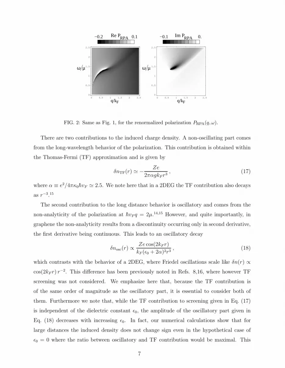
ω = vF q. Figure 2 shows real and imaginary parts of the self-consistent polarization. While

the singularity at ω = vF q is absent, a new singularity appears in RePRPA(q, ω) at ω ∝ √q,

which reflects the existence of plasmons, as will be discussed in subsection IV.

III. STATIC SCREENING

An external charge density next(r) = Zeδ(r) is screened by free electrons due to the

Coulomb interaction. This results in the induced charge density δn(r)

δn(r) =Ze

4π2

∫

d2q

[

1

ǫ(q, 0)− 1

]

eiq·r . (15)

Here ǫ(q, 0) ≡ limω→0 ǫ(q, ω). Within the RPA approximation6

ǫ(q, ω) = ǫ0 − vqP(1)(q, ω) . (16)

The effective dielectric constant ǫ0 includes high energy screening processes. We take ǫ0 ≃2.4.5

6

0 0.5 1 1.5 2 2.50

0.5

1

1.5

2

2.5

0 0.5 1 1.5 2 2.50

0.5

1

1.5

2

2.5

ω µ ω µ

q/kF q/kF

RPA RPA0.1 0.−0.2 −0.1 Re P Im P

FIG. 2: Same as Fig. 1, for the renormalized polarization PRPA(q, ω).

There are two contributions to the induced charge density. A non-oscillating part comes

from the long-wavelength behavior of the polarization. This contribution is obtained within

the Thomas-Fermi (TF) approximation and is given by

δnTF(r) ≃ − Ze

2παgkFr3, (17)

where α ≡ e2/4πκ0hvF ≃ 2.5. We note here that in a 2DEG the TF contribution also decays

as r−3.15

The second contribution to the long distance behavior is oscillatory and comes from the

non-analyticity of the polarization at hvF q = 2µ.14,15 However, and quite importantly, in

graphene the non-analyticity results from a discontinuity occurring only in second derivative,

the first derivative being continuous. This leads to an oscillatory decay

δnosc(r) ∝Ze cos(2kF r)

kF (ǫ0 + 2α)2r3, (18)

which contrasts with the behavior of a 2DEG, where Friedel oscillations scale like δn(r) ∝cos(2kF r) r

−2. This difference has been previously noted in Refs. 8,16, where however TF

screening was not considered. We emphasize here that, because the TF contribution is

of the same order of magnitude as the oscillatory part, it is essential to consider both of

them. Furthermore we note that, while the TF contribution to screening given in Eq. (17)

is independent of the dielectric constant ǫ0, the amplitude of the oscillatory part given in

Eq. (18) decreases with increasing ǫ0. In fact, our numerical calculations show that for

large distances the induced density does not change sign even in the hypothetical case of

ǫ0 = 0 where the ratio between oscillatory and TF contribution would be maximal. This

7

-0.0006

-0.0004

-0.0002

0

1 1.5 2 2.5 3 3.5 4 4.5 5

δn(r

)

kFr / π

-0.024

-0.016

-0.008

0

0 2 4 6 8 10

δn(r

) (k

Fr)

3

kFr / π

FIG. 3: Induced charge density δn(r) (in units of k2F Ze) as a function of the dimensionless variable

kF r/π. The inset shows the r−3 decay at large distances. The high frequency screening is set

to ǫ0 = 2.4. In the used representation the graphs are invariant under a change of the chemical

potential.

remarkable general property can be clearly appreciated in Fig. 3 for the particular case of

ǫ0 = 2.4: The induced density δn(r) does not change sign, but oscillates around a finite

offset.

The polarization also determines the Ruderman-Kittel-Kasuya-Yosida (RKKY) inter-

action energy between two magnetic impurities as well as the induced spin density due

to a magnetic impurity, both quantities being proportional to the Fourier transform of

P (1)(q, 0).17 For a magnetic impurity at r the induced spin density δm(r) is

δm(r) ∝ P (1)(r) =1

4π2

∫

d2q P (1)(q, 0)eiq·r . (19)

Note that the magnetic response is proportional to the bare polarization, since the spin-spin

interaction is mediated via the short ranged exchange interaction (in contrast to the long

ranged Coulomb interaction in the case of charge response). That is why the TF contribution

is missing and the induced spin density oscillates around zero. Figure 4 shows the numerically

calculated P (1)(r) in units of k3F/hvF and illustrates this behavior. Specifically in the long

wavelength limit we obtain

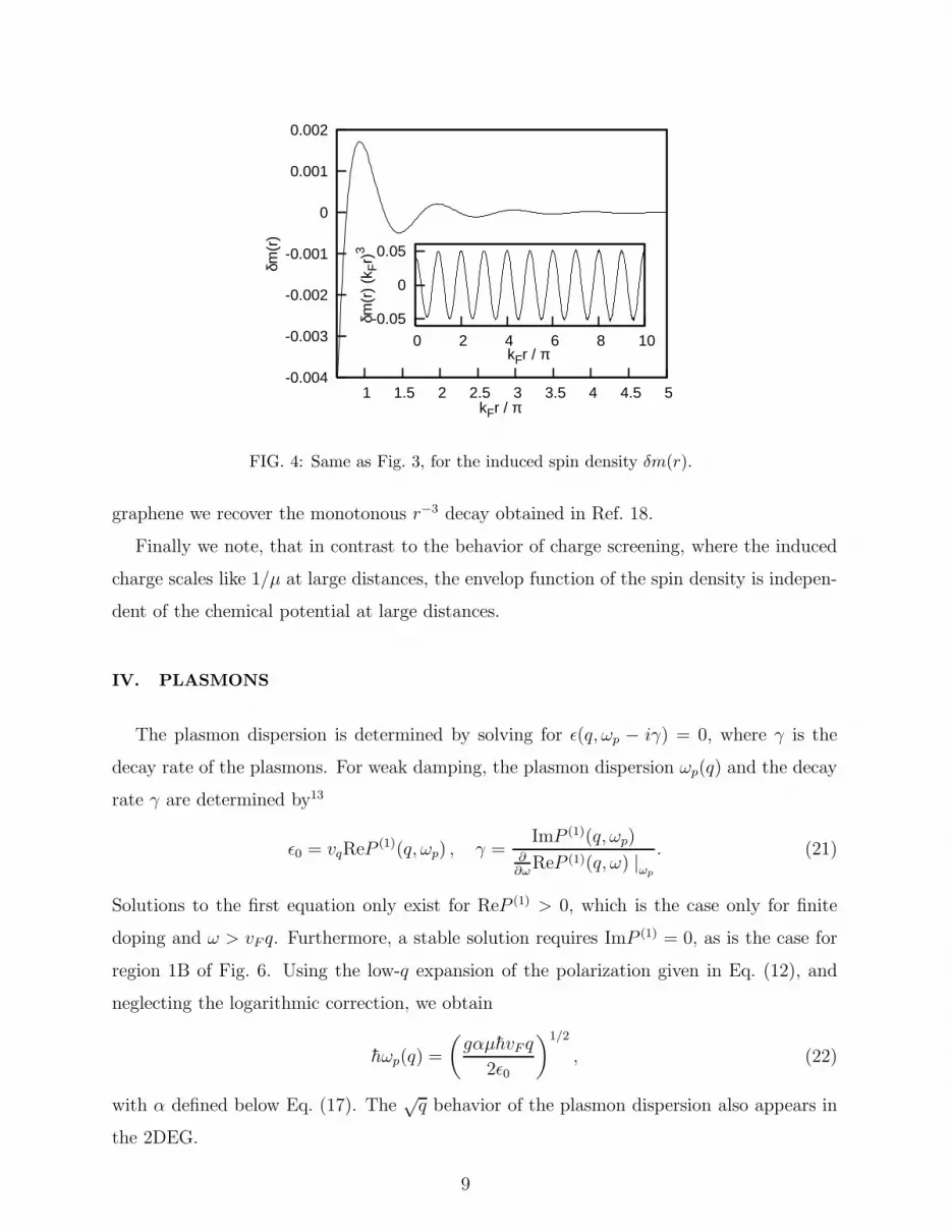
δm(r) ∝ cos(2kF r)

r3, (20)

which is clearly seen in the inset of Fig 4. Like for the induced charge density, we find

that the induced spin polarization δm(r) decreases like r−3 for large distances. Again, this

contrasts with the r−2 behavior found in a 2DEG.17 For the particular case of undoped

8

-0.004

-0.003

-0.002

-0.001

0

0.001

0.002

1 1.5 2 2.5 3 3.5 4 4.5 5

δm(r

)

kFr / π

-0.05

0

0.05

0 2 4 6 8 10

δm(r

) (k

Fr)

3kFr / π

FIG. 4: Same as Fig. 3, for the induced spin density δm(r).

graphene we recover the monotonous r−3 decay obtained in Ref. 18.

Finally we note, that in contrast to the behavior of charge screening, where the induced

charge scales like 1/µ at large distances, the envelop function of the spin density is indepen-

dent of the chemical potential at large distances.

IV. PLASMONS

The plasmon dispersion is determined by solving for ǫ(q, ωp − iγ) = 0, where γ is the

decay rate of the plasmons. For weak damping, the plasmon dispersion ωp(q) and the decay

rate γ are determined by13

ǫ0 = vqReP (1)(q, ωp) , γ =ImP (1)(q, ωp)

∂∂ω

ReP (1)(q, ω) |ωp

. (21)

Solutions to the first equation only exist for ReP (1) > 0, which is the case only for finite

doping and ω > vF q. Furthermore, a stable solution requires ImP (1) = 0, as is the case for

region 1B of Fig. 6. Using the low-q expansion of the polarization given in Eq. (12), and

neglecting the logarithmic correction, we obtain

hωp(q) =

(

gαµhvF q

2ǫ0

)1/2

, (22)

with α defined below Eq. (17). The√q behavior of the plasmon dispersion also appears in

the 2DEG.

9

0.25 0.5 0.75 1 1.25

0.5

1

1.5

2

2.5

0.25 0.5 0.75 1 1.25

0.5

1

1.5

0.2 0.4 0.6 0.8 1 1.2 1.4

0.02

0.04

0.06

0.08

0.1

0.12

0.14

0.2 0.4 0.6 0.8 1 1.2 1.4

0.05

0.1

0.15

0.2

0.25

0.3

ω µ

0ε = 2.4b)0ε = 1

0ε = 1 0ε = 2.4γ µ γ µ

q/kF q/kF

q/kF q/kF

a)

c) d)

ω µ

FIG. 5: Upper row: Solid lines show the dispersion relation for plasmons defined by Re ǫ(q, ω) = 0.

Dotted lines show the low-q expansion of Eq. (22), while the dashed lines represents ω = vF q. The

crosses indicate where the plasmons acquire a finite lifetime. Lower row: Decay rate γ of plasmons

[see Eq. (21)] in units of chemical potential. We set h = 1.

Outside region 1B, the plasmon is damped, i.e. it has a nonzero decay rate γ. This can be

clearly seen in Figs. 2 and 5. In the upper row of Fig. 5, we plot the exact plasmon dispersion

for two different values of ǫ0 and indicate the point at which the collective excitation becomes

damped. The lower row shows the decay rate as obtained from Eq. (21).

Finally, it is interesting to note that the combination of the linear dispersion relation for

quasiparticles [electrons above (or holes below) the Fermi energy] and the plasmon dispersion

makes it impossible for a quasiparticle of energy hω to decay into a plasmon with q ≤ ω/vF .

Hence, plasmons with infinite lifetime do not contribute to the lifetime of quasiparticles.

V. ACOUSTIC PHONONS AND SOUND VELOCITY

We now calculate the dispersion and the decay rate of acoustical phonons in graphene.

We treat the electrons in the π-band of graphene as quasi-free electrons, while all the other

electrons are assumed to be tightly bound to the carbon nuclei, thus forming effective ions

with a positive elementary charge. In the absence of screening by the conduction electrons,

the ions oscillate at their plasma frequency due to the long range nature of the Coulomb

10

interaction. The collective modes of the combined electron-ion plasma can be obtained

from the zeros of the total dielectric function ǫtot(q, ω), which is obtained by summing the

contributions from ions and electrons:19

ǫtot(q, ω) = ǫel(q, ω) + ǫion(q, ω) − 1 = ǫ0 − vq [Pel(q, ω) + Pion(q, ω)] (23)

Here Pel, ǫel are the polarization and the dynamical dielectric function of the electrons as

given in Eqs. (9) and (16), while Pion, ǫion are the corresponding quantities for the ions. In

the calculation of Pion(q, ω) we assume that the ions have a quadratic energy dispersion

E = h2k2/2M where M denotes the ion mass. The ionic charge density is two positive

charges per unit cell, so that the Fermi wave vector of the ions is k′F ≃ (8π/Ac)1/2, where

Ac = 3√

3a2/2 denotes the area of the hexagonal unit cell in real space.11 This value of k′F

is exact for field effect doping and approximate for chemical doping.

In the calculation of Pion we assume that, for all relevant frequencies, we can take ω ≫hk′F q/M . In the case of acoustic phonons this assumption is equivalent to vs ≫ hk′F/M ≃1.3×10−4vF , where vs denotes the sound velocity. This relation is fulfilled for all meaningful

dopings as shown below. In this regime the ion polarization is real and given by

Pion(q, ω) =k′F

2q2

4πMω2=

2E0q2

h2ω2, (24)

where we defined E0 = h2/MAc ≃ 7 × 10−5 eV. We note that E0 is of the order of the ion

confinement energy.

We may estimate the dispersion and the decay rate of the acoustical phonons by inserting

Eq. (23) into Eq. (21). For finite doping µ > 0, the acoustic phonons at long wavelengths

lie in the region 1A of Fig. 6 (defined by ω < vF q < 2µ/h − ω), where ReP (1)(q, ω) =

−gµ/2πh2v2F . In this regime the phonon dispersion is easily obtained:

ωph =

(

4παE0

ǫ0hvF q + gαµ

)1/2

vF q . (25)

To be consistent with the precondition ω < vF q the expression in the square root has to be

smaller than one. This sets a lower limit to the values of the chemical potential for which

Eq. (25) is valid. The sound velocity vs and the decay rate γ may be derived from Eqs. (21)

and (25) in the limit of low q. We obtain

vs =√

ξ vF , γ =ξvF q

2√

1 − ξ, (26)

11

with ξ = 4πE0/gµ.

Some additional remarks on the validity of Eq. (25) go in place. We have already said

that, for q → 0, it only applies provided ξ < 1. We also wish to note that the acoustical

phonons are only well-defined if their frequency is much larger than their decay rate, i.e. if

ωph/γ ≫ 1. Since ωph/γ = 1 for ξ = 4/5, we conclude that the notion of acoustic phonons is

justified for ξ ≪ 1, which corresponds to µ ≫ 4πE0/g ≃ 2.2×10−4 eV. A detailed discussion

of acoustical phonons for ξ > 1 is left for future work.

We have assumed initially that vs ≫ hk′F/M ≃ 1.3× 10−4vF . According to Eq. (26) this

results in ξ ≫ 1.7 × 10−8, or equivalently, µ≪ 108E0, which is always fulfilled.

We finish this section by estimating the sound velocity of a typical graphene sample.

Assuming a concentration of ”conduction-band” electrons of nel = 1010 − 1012 cm−2 we

get µ ≃ 10−2 − 10−1 eV. We note that this corresponds to ξ ≃ 2 − 20 × 10−3, so that

Eqs. (25) and (26) are applicable, resulting in vs ≃ 0.05 − 0.14 vF ≃ 4 − 12 × 104 m/s and

γ ≃ 10−3 − 10−2 vF q. These results suggest a significant enhancement of the sound velocity,

as compared to normal metals, where vs ≃√

m/2MvF<∼ 10−2vF . The low polarizability

of the conduction electrons leads to a poor screening of the oscillations of the charged ions.

On the other hand, in a semiconductor with a gap larger than the typical acoustic phonon

frequencies, the electrons follow adiabatically the ions. In that case, the lattice vibrations

can be described as oscillations of neutral particles.

VI. CONCLUSIONS

In this article we have derived a compact and closed expression for the dynamical po-

larization of graphene within the RPA approximation. The obtained result is valid for

arbitrary wave vector, frequency, and doping. As particular cases, we have derived the long-

wavelength limit q → 0 and the static limit ω → 0. We have employed the RPA polarization

to calculate several physical quantities of interest in doped graphene. First we have stud-

ied the static Friedel oscillations of the induced charge(spin) density in the presence of a

charged(magnetic) impurity. We have found that, although the charge density does show

oscillations around an average value, it does it without changing sign. The reason for this

remarkable behavior is that Friedel oscillations superpose on the dominant Thomas-Fermi

induced density, with both contributions decaying at long distances r with the same power

12

law r−3.

The dynamical polarization has been used to calculate the dispersion relation and the

decay rate of plasmons and acoustic phonons. Like in the 2DEG case, the plasmon frequency

shows a√q-behavior in the long wavelength regime. We have determined the region in the

(q, ω) plane where the plasmon is stable, as well as the decay rate in the regime where it is

not.

The dispersion of acoustical phonons has been shown to be strongly dependent on the

chemical potential. In particular, we have found that the sound velocity approaches the

Fermi velocity at low doping. However, the same limit shows an increase in the decay rate

of acoustic phonons due to electron-hole pair excitation.

Although we have focused on applications of the RPA calculation to the case of doped

graphene, some aspects of the low-frequency, long-wavelength dynamics of pure graphene

appear to be intriguing and worth studying further.

Note added. When this work was about to be submitted, we became aware of a related

paper.21 Overlapping results in the two papers are in agreement.

Acknowledgements

We appreciate helpful discussions with A. H. Castro Neto. This work has been supported

by the EU Marie Curie RTN Programme No. MRTN-CT-2003-504574, the EU Contract

12881 (NEST), and by MEC (Spain) through Grants No. MAT2002-0495-C02-01, FIS2004-

05120, FIS2005-05478-C02-01, the Juan de la Cierva Programme and the Comunidad de

Madrid program CITECNOMIK, ref. CM2006-S-0505-ESP-0337.

APPENDIX A: CALCULATION OF THE POLARIZATION

In the following we present some major steps of the calculation of the polarization. We

restrict the discussion to ω > 0 since P (1)(q,−ω) =[

P (1)(q, ω)]∗

. In all the Appendix we

set vF = h = 1, so that in the Appendix µ = kF .

13

2 µ

ω

q

3 A

2 A

1 A

1 B

2 B

3 B

2 kF

FIG. 6: Display of the different regions characterizing the susceptibility behavior. Regions are

limited by straight lines ω = vF q (solid), ω = vF q−2µ (dashed) and ω = 2µ− vF q (dotted), where

we set h = 1.

1. Imaginary part

The imaginary part of the functions χ±D(q, ω) defined in Eq. (5) has the following form

ImχβD(q, ω) = − g

4π

∫ D

0

dk∑

α=±

α Iαβ(k, q, ω) ,

Iαβ = k

∫ 2π

0

dϕ fβ(k,q)δ [ω + α(k − β|k + q|)] ,

The ϕ-integration yields

Iαβ =

[

(2αk + ω)2 − q2

q2 − ω2

]1

2

{

Θ(β)Θ(q − ω)Θ

(

k − q − αω

2

)

+Θ(−β)Θ(ω − q)Θ(−α)

[

Θ

(

ω + q

2− k

)

− Θ

(

ω − q

2− k

)]}

,

which is always real. The final k-integration can now simply be performed. We obtain for

µ = 0

ImP(1)0 (q, ω) =

g

4π

∫ Λ

0

dk∑

α

α Iα−(k, q, ω) = − gq2

16√

ω2 − q2Θ(ω − q). (A1)

14

In order to present the result for µ > 0, we introduce the real functions f(q, ω), G>(x), G<(x)

f(q, ω) =g

16π

q2

√

|ω2 − q2|,

G>(x) = x√x2 − 1 − cosh−1(x) , x > 1 ,

G<(x) = x√

1 − x2 − cos−1(x) , |x| < 1 . (A2)

For the additional term at finite doping given by Eq. (7), we obtain in the language of Fig. 6

Im∆P (1)(q, ω) = − g

4π

∫ µ

0

dk∑

α,β

α Iαβ(k, q, ω) = f(q, ω)×

G>(2µ−ωq

) −G>(2µ+ωq

) , 1 A

π , 1 B

−G>(2µ+ωq

) , 2 A

−G<(ω−2µq

) , 2 B

0 , 3 A

0 , 3 B

2. Real part

The Kramers-Kronig relation valid for the retarded function ReP(1)0 (q, ω) reads

ReP(1)0 (q, ω) =

1

π

∞∫

−∞

dω′ ImP(1)0 (q, ω′)

ω′ − ω= − gq2

16√

q2 − ω2Θ(q − ω). (A3)

For finite doping we rewrite Eq. (7) as

Re∆P (1)(q, ω) =g

4π2

∫ µ

0

dk k

∫ 2π

0

dϕ∑

α=±

2k + αω + q cosϕ

(k + αω)2 − |k + q|2 .

This integral is calculated directly such that the Kramers-Kronig relation is not needed,

here. The ϕ-integration yields

Re∆P (1) = −gµ2π

+g

8π2

∑

α=±

∫ µ

0

dkJa(k, q, ω), (A4)

where Jα(k, q, ω) is given by

Jα =2π

[

(2αk + ω)2 − q2

ω2 − q2

]1

2

{

Θ(q − ω)Θ(q − αω

2− k)

+Θ(ω − q)

[

Θ(α) + Θ(−α)

(

Θ(ω − q

2− k) − Θ(k − ω + q

2)

)]}

.

15

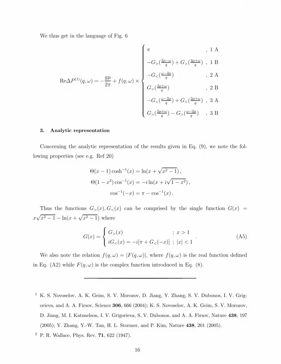
We thus get in the language of Fig. 6

Re∆P (1)(q, ω) = −gµ2π

+ f(q, ω) ×

π , 1 A

−G>(2µ−ωq

) +G>(2µ+ωq

) , 1 B

−G<(ω−2µq

) , 2 A

G>(2µ+ωq

) , 2 B

−G<(ω−2µq

) +G<(2µ+ωq

) , 3 A

G>(2µ+ωq

) −G>(ω−2µq

) , 3 B

3. Analytic representation

Concerning the analytic representation of the results given in Eq. (9), we note the fol-

lowing properties (see e.g. Ref 20)

Θ(x− 1) cosh−1(x) = ln(x+√x2 − 1) ,

Θ(1 − x2) cos−1(x) = −i ln(x+ i√

1 − x2) ,

cos−1(−x) = π − cos−1(x) .

Thus the functions G>(x), G<(x) can be comprised by the single function G(x) =

x√x2 − 1 − ln(x+

√x2 − 1) where

G(x) =

G>(x) ; x > 1

iG<(x) = −i[π +G<(−x)] ; |x| < 1. (A5)

We also note the relation f(q, ω) = |F (q, ω)|, where f(q, ω) is the real function defined

in Eq. (A2) while F (q, ω) is the complex function introduced in Eq. (8).

1 K. S. Novoselov, A. K. Geim, S. V. Morozov, D. Jiang, Y. Zhang, S. V. Dubonos, I. V. Grig-

orieva, and A. A. Firsov, Science 306, 666 (2004); K. S. Novoselov, A. K. Geim, S. V. Morozov,

D. Jiang, M. I. Katsnelson, I. V. Grigorieva, S. V. Dubonos, and A. A. Firsov, Nature 438, 197

(2005); Y. Zhang, Y.-W. Tan, H. L. Stormer, and P. Kim, Nature 438, 201 (2005).

2 P. R. Wallace, Phys. Rev. 71, 622 (1947).

16

3 J. W. McClure, Phys. Rev. 108, 612 (1957).

4 J. Gonzalez, F. Guinea, and V. A. M. Vozmediano, Nucl. Phys. B 424, 595 (1994).

5 T. Ando, J. Phys. Soc. Jap. 75, 074716 (2006); E. V. Gorbar, V. P. Gusynin, V. A. Miransky

and I. A. Shovkovy, Phys. Rev. B 66, 045108 (2002).

6 K. W.-K. Shung, Phys. Rev. B 34, 979 (1986); ibid. 1264 (1986); M. F. Lin and K. W.-K.

Shung,Phys. Rev. B 46, 12656 (1992).

7 D. P. DiVincenzo and E. J. Mele, Phys. Rev. B 29, 1685 (1984).

8 M. I. Katsnelson, cond-mat/0609026.

9 K. Nomura and A. H. MacDonald, cond-mat/0606589

Vafek

10 K. Nomura and A. H. MacDonald, Phys. Rev. Lett. 96, 256602 (2006).

11 N. M. R. Peres, F. Guinea, and A. H. Castro Neto, Phys. Rev. B 73, 125411 (2006).

12 G. D. Mahan, Many-Particle Physics (Plenum, New York, 1990).

13 A. L. Fetter, and J. D. Walecka, Quantum Theory of Many-Particle Systems (Dover, New York,

2003).

14 M.J. Lighthill, Introduction to Fourier Analysis and Generalized Functions (Cambridge Univer-

sity Press, Cambridge, 1958).

15 F. Stern, Phys. Rev. Lett. 18, 546 (1967).

16 V. V. Cheianov and V. I. Fal’ko, cond-mat/0608228.

17 B. Fischer and M. W. Klein, Phys. Rev. B 11, 2025 (1975); M. T. Beal-Monod, Phys. Rev. B

36, 8835 (1987).

18 V. A. M. Vozmediano, M. P. Lopez-Sancho, T. Stauber, and F. Guinea, Phys. Rev. B 72,

155121 (2005).

19 N. W. Ashcroft and N. D. Mermin, Solid State Physics (Holt-Saunders, New York, 1976).

20 M. Abramowitz and I. A. Stegun, Handbook of Mathematical Functions (Dover, New York,

1972).

21 E. H. Hwang and S. Das Sarma, cond-mat/0610561.

17