EPJ B proofs(will be inserted by the editor)

Does roughening of rock-fluid-rock interfaces emergefrom a stress-induced instability?

E. Bonnetier1, C. Misbah2,a, F. Renard3,4, R. Toussaint5,6, and J.-P. Gratier3

1 Laboratoire Jean Kuntzmann, Universite Joseph Fourier and CNRS, B.P. 53, 38041 Grenoble Cedex 9, France2 Laboratoire de Spectrometrie Physique, 140 avenue de la physique, Universite Joseph Fourier, and CNRS, 38402, Saint Martin

d’Heres, France3 Laboratoire de Geodynamique des Chaines Alpines, CNRS-OSUG, Universite Joseph Fourier, B.P. 53, 38041 Grenoble, France4 Physics of Geological Processes, University of Oslo, Norway5 Institut de Physique du Globe de Strasbourg, UMR CNRS 7516, 5 rue Descartes, 67084 Strasbourg Cedex, France6 EOST, Universite de Strasbourg, France

Received 20 October 2008 / Received in final form 24 November 2008Published online (Inserted Later) – c© EDP Sciences, Societa Italiana di Fisica, Springer-Verlag 2008

Abstract. Non-planar solid-fluid-solid interfaces under stress are very common in many industrial andnatural materials. For example, in the Earth’s crust, many rough and wavy interfaces can be observed inrocks in a wide range of spatial scales, from undulate grain boundaries at the micrometer scale, to stylolitedissolution planes at the meter scale. It is proposed here that these initially flat solid-fluid-solid interfacesbecome rough by a morphological instability triggered by elastic stress. A model for the formation of theseunstable patterns at all scales is thus presented. It is shown that such instability is inherently present dueto the uniaxial stress that promotes them, owing to the gain in the total elastic energy: the intrinsic elasticenergy plus the work of the external forces. This is shown explicitly by solving the elastic problem in alinear stability analysis, and proved more generally without having resort to the computation of the elasticfield.

PACS. 91.32.De Crust and lithosphere – 68.35.Fx Diffusion; interface formation – 02.30.Jr Partial dif-ferential equations – Plasticity, diffusion, and creep Plasticity, diffusion, and creep – 91.60.Dc Plasticity,diffusion, and creep

1 Introduction1

When a solid is non-uniformly loaded (Fig. 1), its elas-2

tic free energy is increased and local gradients of free-3

energy can induce mass transfer from the most stressed4

sides of the solid to the least stressed ones, or to other5

surrounding solids, to minimize the energy increase re-6

lated to the loading. The interface kinetics of the stressed7

solid is controlled by the slowest mechanism by which the8

mass is transported. This configuration is found in many9

layered industrial materials or natural systems. For ex-10

ample, in the rocks of the Earth’s crust, loaded interfaces11

are widespread: fault surfaces and stylolites (Fig. 2) at a12

macroscopic scale; grain boundaries and grain free surfaces13

in a porous medium at the microscopic scale.14

Two different geometries can be defined, depending on15

the orientation of the main compressive stress relative to16

the loaded interface (Fig. 1).17

a e-mail: chaouqi.misbah@ujf-grenoble.fr

– When the main compressive stress is parallel to 18

the surface, grooves can develop, this is the 19

Asaro-Tiller-Grinfeld instability [3,11,12,21,23,31], re- 20

ferred to, later in this paper, as “the free-face instabil- 21

ity”. This instability is well understood theoretically. It 22

has been observed on Helium by Torii and Balibar [33]. 23

It has also been proposed that it could be reproduced 24

experimentally on sodium chlorate single crystals [7]. 25

However, experiments on the same salt do also show 26

that this instability may disappear after some time. 27

This effect might be related to the precipitation of a 28

stress-free skin at the surface of the crystals [5]. 29

– When the main compressive stress is perpendicular to 30

the solid surface, initially flat dissolution surfaces can 31

become rough in the course of time by a dissolution 32

process. Typical natural examples of such squeezed 33

unstable interfaces can be observed in natural rocks. 34

They are called stylolites (Fig. 2). In sedimentary 35

basins, stylolites are observed as rough horizontal in- 36

terfaces [8,13,24,30,32]. There, the main compressive 37

insu

-003

5288

6, v

ersi

on 1

- 14

Jan

200

9Author manuscript, published in "The European Physical Journal B 67, 1 (2009) 121-131"

DOI : 10.1140/epjb/e2009-00002-2

2 The European Physical Journal B

stress is vertical and corresponds to the weight of1

the overburden rocks. In mountain chains, where the2

main compressive stress corresponds to the horizontal3

tectonic loading, rough stylolite surfaces are oriented4

vertically [2,25]. From these basic observations, one5

may conclude that stress is a key ingredient in sty-6

lolite pattern formation [4,17]. In the present study,7

we call such roughening process “the squeezed inter-8

face instability”. It differs from the free-face instability9

by the orientation of the main compressive stress. This10

second instability is less understood. It has been pro-11

posed that the roughening of the interface is controlled12

by a destabilizing force, the noise initially present in13

the rock [26,27]. In [9] it was assumed that diffusion oc-14

curs along the solid-solid interface and a simple model15

to describe the instability has been proposed. However,16

a model that takes into account a more realistic geom-17

etry is lacking, together with a systematic derivation18

of the governing equations. Furthermore, it remains to19

be shown whether or not a purely elastic instability20

explains the formation of stylolites. This paper is di-21

rected along these lines.22

We present a model that shows that squeezed solid-fluid-23

solid interfaces are unstable due to stress. This situation is24

less classical than the one usually treated: here two solids25

are in contact with a thin liquid layer and the weight is26

transmitted from one solid to the other by the liquid layer.27

It is thus essential to derive the equations and boundary28

conditions in this geometry. We must take into account29

not only the intrinsic elastic energy but also the work due30

to external forces.31

Natural and experimental observations of rough sur-32

faces indicate that stress has a strong control on the evo-33

lution of the fluid-solid interfaces: stress gradients are re-34

leased by dissolution-precipitation or melting solidification35

processes, which modify the solid texture and induce irre-36

versible deformations (see Fig. 2).37

The scheme of this paper is as follows. In Section 2 we38

briefly review the free interface case. In Section 3 we treat39

the squeezed interface case by performing a linear stabil-40

ity analysis, and present the main results that reveals an41

instability driven by stress. In Section 4 we present a more42

general and formal proof of the instability without having43

resort to an explicit solution of the elastic field. Section 544

is devoted to a general discussion. Some technical details45

are presented in an appendix.46

2 The free interface case47

If the main compressive stress is parallel to the loaded48

interface (Fig. 1a), grooves can develop on the free sur-49

face. This is the well-known Asaro-Tiller-Grinfeld insta-50

bility [3,11]. It has been found experimentally [7,19,33]51

that the formation of the grooves occurs on a free surface52

of various solids in contact with a fluid when a load (or53

a uniaxial stress [33]) is applied. The grooves can theo-54

retically evolve to fractures that propagate at a subcriti-55

cal rate [14,16,18,31,34]. The wavelength of the instability56

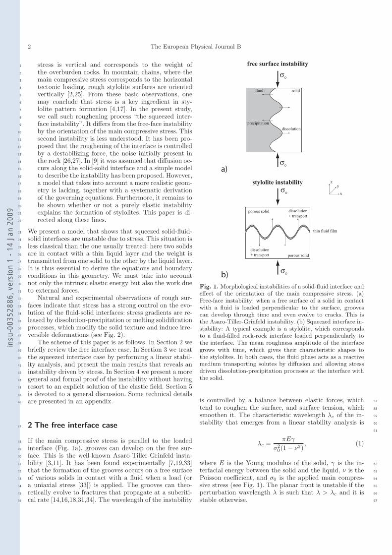
fluid

precipitation

solid

dissolution

x

yz

thin fluid film

porous solid

porous solid dissolution+ transport

free surface instability

stylolite instability

a)

b)

σO

σO

σO

σO

dissolution+ transport

Fig. 1. Morphological instabilities of a solid-fluid interface andeffect of the orientation of the main compressive stress. (a)Free-face instability: when a free surface of a solid in contactwith a fluid is loaded perpendicular to the surface, groovescan develop through time and even evolve to cracks. This isthe Asaro-Tiller-Grinfeld instability. (b) Squeezed interface in-stability: A typical example is a stylolite, which correspondsto a fluid-filled rock-rock interface loaded perpendicularly tothe interface. The mean roughness amplitude of the interfacegrows with time, which gives their characteristic shapes tothe stylolites. In both cases, the fluid phase acts as a reactivemedium transporting solutes by diffusion and allowing stressdriven dissolution-precipitation processes at the interface withthe solid.

is controlled by a balance between elastic forces, which 57

tend to roughen the surface, and surface tension, which 58

smoothen it. The characteristic wavelength λc of the in- 59

stability that emerges from a linear stability analysis is 60

61

λc =πEγ

σ20(1 − ν2)

, (1)

where E is the Young modulus of the solid, γ is the in- 62

terfacial energy between the solid and the liquid, ν is the 63

Poisson coefficient, and σ0 is the applied main compres- 64

sive stress (see Fig. 1). The planar front is unstable if the 65

perturbation wavelength λ is such that λ > λc and it is 66

stable otherwise. 67

insu

-003

5288

6, v

ersi

on 1

- 14

Jan

200

9

E. Bonnetier et al.: Does roughening of rock-fluid-rock interfaces emerge from a stress-induced instability? 3

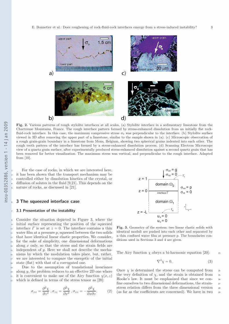
Fig. 2. Various patterns of rough stylolite interfaces at all scales. (a) Stylolite interface in a sedimentary limestone from theChartreuse Mountains, France. The rough interface pattern formed by stress-enhanced dissolution from an initially flat rock-fluid-rock interface. In this case, the maximum compressive stress σ0 was perpendicular to the interface. (b) Stylolite surfaceviewed in 3D after removing the upper part of a limestone, similar to the sample shown in (a). (c) Microscopic observation ofa rough grain-grain boundary in a limestone from Mons, Belgium, showing two spherical grains indented into each other. Therough teeth pattern of the interface has formed by a stress-enhanced dissolution process. (d) Scanning Electron Microscopeview of a quartz grain surface, after experimentally produced stress-enhanced dissolution against a second quartz grain that hasbeen removed for better visualization. The maximum stress was vertical, and perpendicular to the rough interface. Adaptedfrom [10].

For the case of rocks, in which we are interested here,1

it has been shown that the transport mechanism may be2

controlled either by dissolution kinetics of the crystal, or3

diffusion of solutes in the fluid [9,21]. This depends on the4

nature of rocks, as discussed in [21].5

3 The squeezed interface case6

3.1 Presentation of the instability7

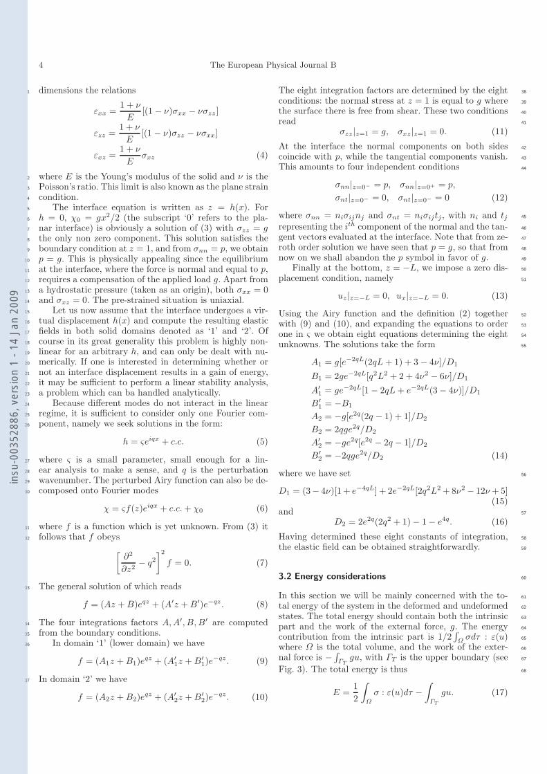
Consider the situation depicted in Figure 3, where the8

initial surface representing the position of the squeezed9

interface Γ is set at z = 0. The interface contains a thin10

water film at a pressure p, squeezed between the two solids11

that have identical linear elastic properties. We consider,12

for the sake of simplicity, one dimensional deformations13

along x only, so that the stress and the strain fields are14

independent of y. Here we shall not describe the mecha-15

nisms by which the modulation takes place, but, rather,16

we are interested to compare the energetic of the initial17

state (flat) with that of a corrugated one.18

Due to the assumption of translational invariance19

along y, the problem reduces to an effective 2D one where20

it is convenient to make use of the Airy function χ(x, z)21

which is defined in terms of the stress tensor as [20]:22

σxx =∂2χ

∂z2, σzz =

∂2χ

∂x2, σxz = − ∂2χ

∂x∂z. (2)

x

z

z = 0

z = 1

z = -L

domain Ω1

domain Ω2

σ = g zz

σ = 0 xz

σ = pnn

σ = 0nt

u = 0 x

u = 0 z

ΓT

interface Γ

ΓB

Fig. 3. Geometry of the system: two linear elastic solids withidentical moduli are pushed into each other and separated bya thin confined water film at pressure p. The boundaries con-ditions used in Sections 3 and 4 are given.

The Airy function χ obeys a bi-harmonic equation [20]: 23

∇4χ = 0. (3)

Once χ is determined the stress can be computed from 24

the very definition of χ, and the strain is obtained from 25

Hooke’s law. It must be emphasized that since we con- 26

fine ourselves to two dimensional deformations, the strain- 27

stress relation differs from the three dimensional version 28

(as far as the coefficients are concerned). We have in two 29

insu

-003

5288

6, v

ersi

on 1

- 14

Jan

200

9

4 The European Physical Journal B

dimensions the relations1

εxx =1 + ν

E[(1 − ν)σxx − νσzz ]

εzz =1 + ν

E[(1 − ν)σzz − νσxx]

εxz =1 + ν

Eσxz (4)

where E is the Young’s modulus of the solid and ν is the2

Poisson’s ratio. This limit is also known as the plane strain3

condition.4

The interface equation is written as z = h(x). For5

h = 0, χ0 = gx2/2 (the subscript ‘0’ refers to the pla-6

nar interface) is obviously a solution of (3) with σzz = g7

the only non zero component. This solution satisfies the8

boundary condition at z = 1, and from σnn = p, we obtain9

p = g. This is physically appealing since the equilibrium10

at the interface, where the force is normal and equal to p,11

requires a compensation of the applied load g. Apart from12

a hydrostatic pressure (taken as an origin), both σxx = 013

and σxz = 0. The pre-strained situation is uniaxial.14

Let us now assume that the interface undergoes a vir-15

tual displacement h(x) and compute the resulting elastic16

fields in both solid domains denoted as ‘1’ and ‘2’. Of17

course in its great generality this problem is highly non-18

linear for an arbitrary h, and can only be dealt with nu-19

merically. If one is interested in determining whether or20

not an interface displacement results in a gain of energy,21

it may be sufficient to perform a linear stability analysis,22

a problem which can ba handled analytically.23

Because different modes do not interact in the linear24

regime, it is sufficient to consider only one Fourier com-25

ponent, namely we seek solutions in the form:26

h = ςeiqx + c.c. (5)

where ς is a small parameter, small enough for a lin-27

ear analysis to make a sense, and q is the perturbation28

wavenumber. The perturbed Airy function can also be de-29

composed onto Fourier modes30

χ = ςf(z)eiqx + c.c. + χ0 (6)

where f is a function which is yet unknown. From (3) it31

follows that f obeys32

[∂2

∂z2− q2

]2

f = 0. (7)

The general solution of which reads33

f = (Az + B)eqz + (A′z + B′)e−qz . (8)

The four integrations factors A, A′, B, B′ are computed34

from the boundary conditions.35

In domain ‘1’ (lower domain) we have36

f = (A1z + B1)eqz + (A′1z + B′

1)e−qz . (9)

In domain ‘2’ we have37

f = (A2z + B2)eqz + (A′2z + B′

2)e−qz . (10)

The eight integration factors are determined by the eight 38

conditions: the normal stress at z = 1 is equal to g where 39

the surface there is free from shear. These two conditions 40

read 41

σzz |z=1 = g, σxz|z=1 = 0. (11)

At the interface the normal components on both sides 42

coincide with p, while the tangential components vanish. 43

This amounts to four independent conditions 44

σnn|z=0− = p, σnn|z=0+ = p,

σnt|z=0− = 0, σnt|z=0− = 0 (12)

where σnn = niσijnj and σnt = niσijtj , with ni and tj 45

representing the ith component of the normal and the tan- 46

gent vectors evaluated at the interface. Note that from ze- 47

roth order solution we have seen that p = g, so that from 48

now on we shall abandon the p symbol in favor of g. 49

Finally at the bottom, z = −L, we impose a zero dis- 50

placement condition, namely 51

uz|z=−L = 0, ux|z=−L = 0. (13)

Using the Airy function and the definition (2) together 52

with (9) and (10), and expanding the equations to order 53

one in ς we obtain eight equations determining the eight 54

unknowns. The solutions take the form 55

A1 = g[e−2qL(2qL + 1) + 3 − 4ν]/D1

B1 = 2ge−2qL[q2L2 + 2 + 4ν2 − 6ν]/D1

A′1 = ge−2qL[1 − 2qL + e−2qL(3 − 4ν)]/D1

B′1 = −B1

A2 = −g[e2q(2q − 1) + 1]/D2

B2 = 2qge2q/D2

A′2 = −ge2q[e2q − 2q − 1]/D2

B′2 = −2qge2q/D2 (14)

where we have set 56

D1 = (3− 4ν)[1 + e−4qL] + 2e−2qL[2q2L2 + 8ν2 − 12ν + 5](15)

and 57

D2 = 2e2q(2q2 + 1) − 1 − e4q. (16)

Having determined these eight constants of integration, 58

the elastic field can be obtained straightforwardly. 59

3.2 Energy considerations 60

In this section we will be mainly concerned with the to- 61

tal energy of the system in the deformed and undeformed 62

states. The total energy should contain both the intrinsic 63

part and the work of the external force, g. The energy 64

contribution from the intrinsic part is 1/2∫

Ω σdτ : ε(u) 65

where Ω is the total volume, and the work of the exter- 66

nal force is − ∫ΓT

gu, with ΓT is the upper boundary (see 67

Fig. 3). The total energy is thus 68

E =12

∫Ω

σ : ε(u)dτ −∫

ΓT

gu. (17)

insu

-003

5288

6, v

ersi

on 1

- 14

Jan

200

9

E. Bonnetier et al.: Does roughening of rock-fluid-rock interfaces emerge from a stress-induced instability? 5

It will be shown in Section 4 that minimization of this en-1

ergy with respect to u yields the appropriate elastic equa-2

tions, div(σ) = 0 and the boundary conditions (11), (12),3

and (13). Upon substitution of the equilibrium condition,4

the relaxed elastic energy will then take the following form5

6

E0 = −12

∫Ω

σ : ε(u)dτ (18)

where the subscript ‘0’ is to remind us that the quantity7

under consideration is the relaxed energy. That this quan-8

tity is negative is obvious, since the relaxed energy should9

be smaller than the non-relaxed one, otherwise there is a10

trivial solution which would have a zero energy, the one11

corresponding to a zero displacement.12

It remains now to be shown that the variation of this13

quantity with respect to an interface modulation ς cos(qx)14

(produced due to some mass transport) is negative, a sig-15

nature of the instability. A general proof is presented in16

Section 4 without resorting to the explicit form of the elas-17

tic field. It is also of interest to have an explicit expression18

of the energy, (and possibly of the chemical potential), if19

one wishes to study the kinetics of the instability, and20

provide the appropriate length and time scales of the evo-21

lution.22

We should remind that σ has a zeroth order contribu-23

tion due to pre-strain, and in computing the energy E024

one has to subtract the energy of the pre-strained state,25

so that the obtained form contains the contribution due26

to the profile z = h(x, t). In the linear regime of pertur-27

bation with respect to h (i.e. the stress is computed up28

to order h), the energy E0 assumes a quadratic form. In29

the general situation where the extent of the upper and30

lower parts of the sample is finite the energy is lengthy31

enough so we did not feel it worthwhile to list it here. We32

give only the limit where qL � 1 (lower part, below the33

interface, is large in comparison to lengths of interest):34

E0 = qg2 1 + ν

ED2

{(1 − 2ν)

[1 + e4q − 2e2q − 4q2e2q

]−4qe2q + e4q − 1

}ς2 (19)

where D2 is a constant defined in equation (16). The above35

energy is computed per unit period along x and per unit36

length along y. If the surface energy (39) is taken into ac-37

count, one has to supplement E0 with the following con-38

tribution39

Es = γ

∫dx

(dh

dx

)2

(20)

where we have used the approximation of small pertur-40

bation so that the change of arclength from the planar41

surface configuration is approximated by (dh/dx)2. The42

cost in surface energy per unit period and unit length in43

the y direction is thus given by44

Es = γq2ς2. (21)

It can be checked that the right hand side in equation (19)45

is always negative, signaling an instability. Note that if the46

work of the external forces in (17) is not included, then47

the relaxed energy would be the opposite of (18), and 48

therefore E0 would have been positive in equation (19), 49

signaling a stability instead of instability. This will fur- 50

ther be shown in the general treatment in Section 4. In 51

contrast to elasticity, the surface energy is stabilizing. A 52

remark is in order. The comparison of the elastic energy 53

(which is destabilizing) and the surface energy (which is 54

stabilizing) has also a similar spirit as that due Griffith in 55

fracture theory. Indeed, in Griffith theory a crack propa- 56

gates if its length � exceeds a typical value given by the 57

ratio of the loss of surface energy γ over the gain in elas- 58

tic energy (crack releases stored elastic energy) ∼σ20/E. 59

More interesting is that the Griffith condition, according 60

to which a crack propagates when its length exceeds a crit- 61

ical length �c, is precisely (apart from a numerical factor 62

of order unity) the condition of the ATG instability: the 63

planar front is unstable if the wavelength is larger than 64

λc (see Eq. (1)), whereas the Griffith condition states [20] 65

that a crack propagates if its length � > �c = (4/π2)λc. 66

We shall first discuss the two extreme limits of large 67

and short wavenumbers. In these extreme limits the ex- 68

pression takes a very simple form. The first case is, per- 69

haps, the most relevant one for natural systems such as 70

stylolites, where we assume that q � 1 (short wavelength). 71

This means that we take the limit where the modulation 72

wavelength is small as compared to the interface extent. 73

The energy (per unit period) takes then the form 74

E0 = −4(1 − ν2)E

|q|g2ς2 (22)

which is negative, signaling a morphological instability. 75

Note that we keep |q| in the expression above in order to 76

stress the nonlocal character of the elastic field. Indeed, in 77

real space the quantity |q| leads to a Hilbert transform of 78

∂xh(x). More precisely 79

TF−1(|q|hq) = (1/π)P∫

∂x′h(x′)x′ − x

, (23)

where TF stands for a Fourier transform, and hq = 80

TF−1(h) (TF−1 designates the inverse Fourier trans- 81

form). The symbol P refers to the fact that the integral 82

must be taken in the sense of the Cauchy principal value. 83

For a real function f(x) the Cauchy principal value is de- 84

fined as 85

P∫ ∞

−∞

f(x)x

dx ≡ limε→0

[∫ −ε

−∞

f(x)x

dx +∫ ∞

ε

f(x)x

dx

].

(24)Let us abbreviate this expression as pv(f(x)/x). Apply- 86

ing TF on both sides of (23), one gets on the left hand 87

side |q|hq, while the right hand side is a convolution pro- 88

viding a product of TF (∂x′h(x′)) and TF (pv(1/(x′ − x)). 89

The first term yields iqhq, while the second one is equal 90

to −iπ sgn(q) (a classical result of theory of distributions, 91

and can easily be obtained by using the residue theorem), 92

sgn(q) stands for ‘sign of q’. The final result (after ac- 93

counting for the factor π in (23)) is q sgn(q)hq = |q|hq, 94

that is identical to the left hand side result. 95

insu

-003

5288

6, v

ersi

on 1

- 14

Jan

200

9

6 The European Physical Journal B

In the opposite limit (q � 1) one gets (for L = 1)1

E0 = − 2(1 + ν)15E(1− ν)

g2q2(17 − 32ν)ς2. (25)

The effect of the confinement leads to a spectrum which2

begins with q2 instead of q. This may have, in principle,3

some significant consequences, as discussed below.4

For example, in the non-confined regime the elastic en-5

ergy (which is ∼q) dominates at small q in comparison to6

the surface energy which behaves as q2. This means that7

the instability is always present there. The typical length-8

scale of the instability is given by balancing the elastic9

energy ∼qg2/E with the surface energy ∼γq2 where γ is10

the surface energy. This leads to a typical length scale11

λc ∼ Eγ/g2.12

In the confined regime the energy behaves as −q2g2�E13

(where for homogeneity reasons we have reintroduced a14

length scale � representing a typical length of the verti-15

cal extent of the solid), precisely like the surface energy16

regarding the q dependence, +q2γ. Since the latter is sta-17

bilizing, while the former is destabilizing, an instability18

may take place only if � > γE/g2. g has a dimension of E19

and can be written as g = nE where n is a dimensionless20

number smaller than one. We must have then � > γ/(nE).21

In most cases γ/E is of the order of an atomic length and22

n is small enough so we conclude that for all practical23

purposes the instability takes place.24

4 A general framework25

In this section, we cast the previous calculation in the26

framework of a variational analysis. We provide a rigor-27

ous mathematical derivation on the stress-induced insta-28

bility. Unlike the previous derivation, the present result29

will be obtained without knowing the explicit expression30

of the elastic field. We restrict ourselves to a 2D situa-31

tion for simplicity; however, the analysis carries over to32

the 3D case. We consider a configuration similar to that33

of Figure 3: a portion of interface Γ separates two pieces34

of solids Ω1 and Ω2 in the rectangle Ω = Ω1 ∪ Ω2 ∪ Γ .35

4.1 Mechanical equilibrium for a fixed interface Γ36

We view the rectangle Ω = (0, 1) × (0, 1) as a small slab37

of solid around an interface and assume periodic bound-38

ary conditions on the vertical sides ΓV = {0} × (0, 1) ∪39

{1} × (0, 1). We assume that Ω1 lies below Ω2 and that40

both are sufficiently regular open sets (say with Lipschitz41

boundaries). A vertical load with modulus g is applied to42

the top boundary ΓT and the displacement u1 is fixed on43

the bottom boundary ΓB . We use the Einstein summation44

convention of repeated indices.45

The transmission conditions between Ω1 and Ω2 mod-46

els the presence of a very thin layer of fluid in the interface.47

We assume therefore that the stress tensors σ1 and σ2 in48

Ω1 and Ω2 satisfy49

σini = pni, on Γ, i = 1, 2,50

where ni denotes the outward normal to Ωi, and where p is 51

the Lagrange multiplier that denotes the (unknown) pres- 52

sure in the thin layer of fluid. Altogether, the mechanical 53

equilibrium of the system is expressed by the equations 54

⎧⎪⎪⎪⎪⎪⎨⎪⎪⎪⎪⎪⎩

−div(σi) = 0 in Ωi,σi = Aε(ui) in Ωi,

σ2n2 = gn2 on ΓT ,u1 = 0 on ΓB,ui periodic on ΓV ,

σini = pni on Γ,

(26)

where i = 1, 2, ε(u) = 1/2(∇u + ∇uT ) is the symmetric 55

strain tensor, and A is the 4×4 tensor of isotropic Lame co- 56

efficients of the solid. Alternatively, the above partial dif- 57

ferential equations can be obtained as the Euler Lagrange 58

equations of the following energy functional 59

EΓ (v1, v2) =12

∫Ωi

Aε(vi) : ε(vi)dx −∫

ΓT

gn2v2. 60

The set V of admissible displacements VΓ consists of pairs 61

(v1, v2) : Ω1 × Ω2 −→ R2 ×R2 of square integrable func- 62

tions, with square integrable derivatives, such that 63

⎧⎨⎩

v1 = 0 on ΓT

v1, v2 periodic on ΓV∫Γ

v1n1 + v2n2 = 0.64

Note that the constraint on the normal displacements 65

on Γ is associated with the Lagrange multiplier p in- 66

troduced above. One easily checks that minimizing EΓ 67

over VΓ yields a solution (u1, u2) to the corresponding 68

Euler-Lagrange equation (26), which is defined up to a 69

horizontal translation of u2. To obtain a well-defined so- 70

lution we further impose the normalization condition 71

∫ΓT

u2

(10

)= 0. 72

4.2 First variation with respect to the interface Γ 73

In this paragraph, we compute the shape derivative, with 74

respect to variations of the interface Γ , of the elastic en- 75

ergy functional 76

J(Γ ) = min(v1,v2)∈V (Γ )

EΓ (v1, v2). 77

Denoting (u1, u2) the solution of the above variational 78

problem (the actual elastic displacements for the geometry 79

defined by the interface Γ , under the loading g) using (26), 80

and integrating by parts shows that 81

J(Γ ) =12

∫Ωi

Aε(ui) : ε(ui)dx −∫

ΓT

gn2u2

= −12

∫Ωi

Aε(ui) : ε(ui) (27)

= −12

∫ΓT

gn2u2. (28)

insu

-003

5288

6, v

ersi

on 1

- 14

Jan

200

9

E. Bonnetier et al.: Does roughening of rock-fluid-rock interfaces emerge from a stress-induced instability? 7

To differentiate the functional with respect to variations1

of the shape of Γ , we follow the approach of Murat and2

Simon [22,28] which we now briefly recall: Consider per-3

turbations of an open set ω ⊂ R2 of the form4

ωt = ω + tθ,5

where θ : R2 −→ R2 is a sufficiently smooth function, and6

t is a small real parameter (the limit t → 0 will be taken7

eventually).8

Let z be a smooth function and consider the function-9

als, defined respectively as a volume integral and a surface10

integral11

J1(ω) =∫

ω

z(u)12

J2(ω) =∫

∂ω

z(u),13

where u is the solution of a partial differential equation14

Au = 0 in ω, with boundary conditions Bu = 0. The15

shape derivatives (or functional derivatives) of J1, J2 in16

the direction θ are defined by17

J ′i(ω)θ = lim

t→0

Ji(ω + tθ) − Ji(ω)t

.18

When ω and u are sufficiently smooth, one can show that19

Ji(ω + tθ) = Ji(ω) + tJ ′i(ω)θ + o(t||θ||), and further, that20

J ′1(ω)θ =

∫ω

∂uz(u)u′ +∫

∂ω

z(u)θn, (29)

J ′2(ω)θ =

∫∂ω

∂uz(u)u′

+∫

∂ω

[Hz(u) + ∂nz(u)]θn, (30)

where ∂nf(x) = ∇f(x)n is the normal derivative of f . The21

presence of the mean curvature H on ∂ω in the derivative22

of the surface integral J2 results from taking variations of23

the surface measure. In these expressions, the local deriva-24

tive u′ of u at x ∈ ω is defined by25

u′(x) = limt→0

ut(x) − u(x)t

,26

where ut is the solution to Au = 0 in ωt with the boundary27

conditions Btut = 0.28

In our context, we consider perturbations (Ω1, Ω2) of29

the form30

Ωti = Ωi + tθ(x, y), i = 1, 2,31

where θ : R2 −→ R2 is sufficiently smooth. We assume32

that θ leaves the outer boundary ∂Ω fixed, (i.e., θ only33

modifies the shape of the interface) and that it preserves34

the volume of each subdomain Ωi35

{θ(x, y) = 0 on ∂Ω|Ωt

i | = |Ωi| i = 1, 2,(31)

which imposes that 36∫Γ

θni = 0. (32)

Let (ut1, u

t2) denote the solution to (26) for the configura- 37

tion Ωt 38⎧⎪⎪⎪⎨⎪⎪⎪⎩

div(Ae(uti)) = 0 in Ωt

iut

1 = 0 on ∂Ωi ∩ ΓB

A∇ut2 n2 = g n2 on ΓT

uti periodic on ΓV

Ae(uti)nt

i = pt nti, on Γ + tθ.

i = 1, 2. (33)

The local derivatives (u′1, u

′2) satisfy 39

div (Ae(u′i)) = 0 in Ωi (34)

and are periodic on the sides ΓV . The boundary condi- 40

tion (26.d) implies that u′1 + θn∂nu1 = 0 on ΓB, which, 41

given the hypothesis on θ, reduces to 42

u′1 = 0 on ΓB. (35)

In the Appendix, we derive the expression of the shape 43

derivative of J(Γ ) . If Γ ⊂ (0, 1) × (0, 1) is a periodic 44

simple curve, sufficiently smooth, one obtains 45

J ′(Γ )θ =12

∫Γ

[Aε(u1) : ε(u1) − Aε(u2) : ε(u2)]θn1

−∫

Γ

p [div(u1) − div(u2)] θn1. (36)

In particular, if Γ is the flat interface Γ 0 = (0, 1) × {y0}, 46

the associated displacements are linear: 47

ui(x, y) = (0,g

λ + 2μy), i = 1, 2. 48

This greatly simplifies the computations (for instance all 49

the terms on Γ0 involving curvature vanish) and one finds 50

in (36) that J ′(Γ0)θ = 0 for any θ, i.e., the flat interface 51

is a local extremum of the elastic energy functional J . 52

We show below that the sign of the second derivative of 53

J with respect to the interface shape variation tells if the 54

extremum is a minimum or a maximum of the energy func- 55

tional. 56

4.3 Second variation with respect to Γ 57

With the notations of the previous section, the second 58

derivative (with respect to the interface shape variation) 59

of a volume integral is given by [29] 60

J ′′1 (ω, θ, θ) = (J ′

1)′(ω, θ, θ) − J ′

1(ω)(∇θ)θ

= limt→0

J ′1(ω + tθ)θ − J ′

1(ω)θt

− J ′1(ω)(∇θ)θ.

If ω and θ are sufficiently smooth, Simon [29] has shown 61

that 62

J1(ω + tθ) = J1(ω) + tJ ′1(ω)θ 63

+t2

2J ′′

1 (ω, θ, θ) + o(t2||θ||). 64

insu

-003

5288

6, v

ersi

on 1

- 14

Jan

200

9

8 The European Physical Journal B

For our objective functional in the form J(Γ ) =1

−1/2∫

ΩiAε(ui) : ε(ui), calculations similar to those pre-2

sented in the Appendix show that at Γ = Γ 03

J ′′(Γ0, θ, θ) = −2∫

Ωi

Aε(u′i) : ε(u′

i), (37)

which is negative, since the elastic densities Aε(u′i) : ε(u′

i)4

are quadratic and positive, and since the fields u′i do not5

vanish identically. We can thus conclude that when t is6

small enough7

J(Γ0 + tθ) = J(Γ0) + J ′(Γ0)θ + J ′′(Γ0, θ, θ) + O(||θ||2)8

< J(Γ0).9

In other words, any variation away from the flat inter-10

face decreases the value of the total elastic energy, which11

demonstrates the instability of the flat interface. Had we12

disregarded the work due to the external force g in equa-13

tion (27), we would then have obtained an opposite sign14

(namely + 12

∫Ωi

Aε(ui) : ε(ui)) for the relaxed energy, and15

thus stability would have been implied.16

Finally if the boundary conditions at the bottom sur-17

face were different, we may ask the question regarding18

sensitivity of our conclusion. If, instead of imposing a zero19

displacement at the bottom surface, we apply a fixed load,20

as for the upper surface, the conclusion about stability is21

unchanged. Let us call h the load, then one has to add22

to (27) the following term − ∫ΓB

hn1v1, then following ex-23

actly the same manipulations as with the last term in (27)24

we arrive at the same final conclusion (37). It would be in-25

teresting to investigate in the future more general bound-26

ary conditions in order to extract the generic conditions27

that trigger an instability.28

5 Discussion29

5.1 Effect of external work on the calculation30

of the total energy31

A point which is worth mentioning is that in writing the32

total energy, we must include both the intrinsic elastic33

energy and the work due to the external forces. Careless-34

ness (for example not including the work done by surface35

forces) would be penalized by a fallacious conclusion: the36

surface would be stable! A simple argument that the ex-37

ternal forces must be included is that when we perform a38

variation of the energy with the respect to the displace-39

ment field we must arrive to the appropriate bulk (Lame40

equation) and boundary conditions, otherwise, the consid-41

ered equations would not fulfill mechanical equilibrium.42

This requirement has guided our considerations.43

5.2 Kinetics effects44

By comparing the final state to the initial one, we did45

not include, de facto, explicitly the notion of kinetics. It is46

quite clear that two mechanisms play a major role: disso- 47

lution and diffusion in the fluid interstices. This has been 48

treated for the free surface case where it has been shown 49

that both dissolution and diffusion may be limiting fac- 50

tors for rocks [21]. We are planning to include diffusion in 51

the fluid layer, and due to the thin fluid layer, it is likely 52

that diffusion should have a two dimensional character 53

(i.e. like surface diffusion; the diffusion constant should 54

then be renormalized by the fluid layer). We expect the 55

spectrum for the surface fluctuation of diffusion to scale 56

like D�2q4, where � is the fluid thickness, and D is the 57

bulk diffusion constant in the liquid. By comparing to the 58

usual diffusion limited spectrum Dq2, the effective diffu- 59

sion should be lowered by a factor of the order of q� � 1 60

(wavelengths of stylolites are usually much bigger than the 61

fluid thickness). 62

For example, it has been found in [21] for quartz and 63

other rocks that the dissolution is the slowest mechanisms. 64

Now due to the thin fluid layer, we expect diffusion to 65

compete, if not to limit, the instability. We hope to report 66

along these lines in the near future. 67

5.3 Chemical potential considerations 68

We translate now the energy calculations performed in 69

the previous sections in terms of chemical potential, for 70

the sake of future kinetic calculations. The chemical po- 71

tential of a solid element at the interface is obtained from 72

the energy change with respect to the interface variation. 73

This corresponds to the cost in energy that is needed to 74

create a bump (a volume element) on the interface. More 75

precisely, let ET denote the sum of the elastic and sur- 76

faces energies, then the very definition of the change of 77

the chemical potential is 78

ΔμT = −δET

δV(38)

where δ denotes the functional derivative (derivative with 79

respect to the interface shape variation). Since we limit 80

ourselves to a one dimensional interface, the functional 81

derivative corresponds to variation with respect to the in- 82

terface profile h(x). It follows that the added (or removed) 83

volume element becomes an area element given by δhdx, 84

where dx is a fixed interval along the x direction. Thus 85

the chemical potential will be just proportional to − δET

δh . 86

The surface energy per unit length along the y direction 87

reads 88

Es = γ

∫ ⎛⎝

[1 +

(dh

dx

)2]1/2

− 1

⎞⎠ dx (39)

and its variation with respect to the profile h(x) is given 89

by 90

δEs = −γ

∫d

dx

⎛⎜⎜⎜⎜⎜⎝

dh

dx[1 +

(dh

dx

)2]1/2

⎞⎟⎟⎟⎟⎟⎠

dx = −γ

∫κdxδh

(40)

insu

-003

5288

6, v

ersi

on 1

- 14

Jan

200

9

E. Bonnetier et al.: Does roughening of rock-fluid-rock interfaces emerge from a stress-induced instability? 9

where we have set1

κ = −d2h

dx2[1 +

(dh

dx

)2]3/2

(41)

which is nothing but the interface curvature. It follows2

that the contribution to the chemical potential from sur-3

face energy is given by4

Δμs = −δET

δV= γκ. (42)

The contribution coming from elasticity is more subtle,5

since the elastic energy is defined in the bulk, while our6

wish is to define a surface chemical potential. It turns out7

that one may express the variation of the elastic energy8

with respect to the interface shape precisely as an integral9

over the surface, as written above for the surface energy10

in equation (40). The calculation is given in details in11

Section 4, and the desired result of the first variation is12

given by equation (36). In that section please note that13

δh used above is equivalent to θ multiplied by the normal14

vector; actually only normal displacements cause a shape15

change. The change in chemical potential due to stress is16

thus given by17

Δμe = −12

[Aε(u1) : ε(u1) − Aε(u2) : ε(u2)]

+ p [div(u1) − div(u2)] (43)

where we recall that ui (i = 1, 2) is the displacement field18

in medium i (see Fig. 3), ε is the deformation (or strain)19

tensor given by ε(u) = (∇u + ∇uT )/2, and A is the fourth20

order tensor which enters Hooke’s law, namely the stress21

tensor σ is related to the deformation by σ = Aε (Aijkl =22

λδikδjl +μδilδjk where λ and μ are the Lame coefficients).23

Finally p is a Lagrange multiplier introduced in Section 4,24

and plays the role of a pressure like term of the thin fluid25

layer, but it must be solved for in a consistent manner, as26

we have seen in Section 4. We have seen that only in the27

linear regime p coincides with the load g.28

Note that if there was only one solid bounded by vac-29

uum, or by a liquid, then the chemical potential would30

simply be given by31

Δμe =12Aε(u) : ε(u) (44)

as has been used in other contexts (see for example [14]).32

Once the total chemical potential is obtained one can33

relate it to the kinetics of the interface. The most sim-34

ple example is that the normal velocity is proportional to35

minus the chemical potential drop across the interface.36

The surface evolution equation (at global equilibrium,37

as is the case in this problem) – or more precisely the38

normal velocity of the interface – vanishes if the chemical39

potential difference vanishes, or equivalently if the energy40

derivative with respect to the shape vanishes. The second41

variation of the energy with respect to the interface shape 42

(which is computed in this paper) is proportional to the 43

variation of the chemical potential Δμ. It is the second 44

variation of energy with respect to the shape that carries 45

information on stability. 46

There are three major physical effects that drive the 47

surface evolution: (i) if the interface is in contact with 48

a reservoir of a liquid containing the molecules of the 49

solid, and if one disregards diffusion (say if the attache- 50

ment/detachment at the surface is the limiting mecha- 51

nism), then the normal velocity is proportional to the 52

chemical potential difference between two states (say the 53

actual one and the initially flat one), this is the case 54

treated in reference [14], (ii) if the surface dynamics 55

evolves due to surface diffusion (as is probably the case 56

for stylolites), then the surface velocity is proportional to 57

the minus of the Laplacian of the chemical potential drop 58

across the interface ΔμT . This is the case treated in Asaro- 59

Tiller [3], and Yang and Srolovitz [34]. The conclusion 60

about stability is the same in both cases, the difference 61

is encoded in the proportionality pre-factor (which has 62

the same sign in both cases) between the normal velocity 63

and the second derivative of the energy with respect to the 64

shape. (iii) Finally if diffusion in the bulk is included, then 65

the normal velocity will be given by an integral equation, 66

and the Kernel of the integral operator, is proportional to 67

ΔμT times a propagator (Green’s function). The propaga- 68

tor expresses the fact that the dynamics becomes nonlocal 69

(addition of mass at some point at the surface is felt by 70

the molecules in the solution at a distant point-due to 71

depletion-inducing thus a nonlocal self-interaction of the 72

moving boundary). But in all the three cases, the insta- 73

bility is encoded in the sign of the second derivative of the 74

energy (with respect to the interface shape). Of course the 75

precise way the instability evolves later in time, depends 76

on the kinetic mechanisms, but not the existence of the 77

instability itself. 78

5.4 Instability of solid-solid interfaces: application 79

to stylolites 80

Solid-solid interface roughening has also been studied, 81

e.g. [1,12], where the two solids have different elastic mod- 82

uli. There, it was demonstrated that an instability can 83

emerge only if the two solids have different material prop- 84

erties. This markedly differs from our situation where the 85

instability does occur even when the two solids have identi- 86

cal elastic properties. This is traced back to the very differ- 87

ence of the two models: in our case it is the thin fluid layer 88

that transmits the stresses and materializes the interface, 89

while in [12], the interface notion looses its meaning if the 90

two solids have identical material properties (Eqs. (22) 91

and (23) in [12] implies that the elastic energy vanishes 92

exactly for χ = 1, i.e. for identical material properties). 93

The present model considers a geometry which is close 94

to that of a natural stylolite, where the interface sepa- 95

rates two pieces of rock, and is a medium of dissolution in 96

a fluid phase. Quantitative measurements on stylolite sur- 97

faces, using a high resolution profilometer, demonstrate 98

insu

-003

5288

6, v

ersi

on 1

- 14

Jan

200

9

10 The European Physical Journal B

that roughening do occur at all scales [27]. The inter-1

pretation of this observation is still controversial. It has2

been proposed that the roughening may be driven by a3

quenched noise initially present in the rock [6,27]. Here, we4

propose an alternative mechanism: stylolite might be in-5

herently unstable, and the roughening could be driven by6

local gradients of strain energy. This interpretation is sup-7

ported by the observation that stylolite do roughen even8

in very pure rocks such as chalk, where the amount of het-9

erogeneities (quenched noise) is very low. However, further10

studies, together with laboratory experiments (mimicking11

the phenomenon) are needed before drawing more conclu-12

sive answers.13

6 Conclusion14

We have shown that a normal load on a solid-fluid-solid15

interface leads to an instability when using a boundary16

condition of transmission of the normal stress, but not17

the shear stress, across the interface. We have shown both18

explicitly (from linear theory with regard to the perturba-19

tion of a flat interface) and from a more general consider-20

ation (still within linear perturbation, but without having21

resort to an explicit solution of the elastic field) that the22

flat interface is unstable.23

When comparing the final state corresponding to a24

modulated surface with the initial state having a flat25

surface, we have shown that the modulated surface has26

lower energy. Given this fact, and the fact related to the27

Asaro-Tiller-Grinfeld instability, it is appealing to specu-28

late that this should be the case in an arbitrary geometry29

and arbitrary boundary conditions, provided that locally30

the considered moving interface possesses a non zero de-31

viatoric stress component. A mathematical general proof32

is still lacking.33

It must be kept in mind that the present study has34

introduced two simplifications. (i) The instability wave-35

length is small as compared with the lateral extent of the36

interface. This holds for natural interfaces that can be37

found in rocks, for example stylolites. If it occurs (in some38

special situation) that this is not the case, then one has39

to consider the role of lateral boundaries as well. (ii) We40

have considered a uniaxial stress and not a bi-axial one as41

occurs in realistic situations. Extensions to more general42

biaxial pre-stress would be interesting.43

Finally, our study has focused on the birth of instabil-44

ity and on the lengthscales that are likely to grow first.45

Nonlinear effects should become decisive in the course of46

time as linear theory tells us that the amplitude should47

grow exponentially with time. How would the final state48

(if any) look like? How would coarsening (if any) occur,49

in that how fast is it? These question require a numerical50

study, and an appropriate way would be to make use of a51

phase-field model, like in [15].52

We acknowledge financial support from the French ministry of53

research (PPF Dynamique des Systemes Complexes). The sup-54

port of Region Rhone Alpes (project Elasticite et Nanostruc-55

tures) and of the ANR project Geocarbone are also gratefully 56

acknowledged. 57

Appendix A: Proof of formula (36) 58

We first recall that the local derivatives u′i are x-periodic 59

on ΓV and that u′1 ≡ 0 on ΓB. Taking the shape deriva- 60

tive (29) of the expression (27) of the objective functional, 61

we obtain 62

J(Γ )′θ = −∫

Ωi

Aε(ui) : ε(u′i) 63

−12

∫∂Ωi

Aε(ui) : ε(ui) θni. 64

Integrating by parts and using the fact that θ vanishes on 65

the boundaries but on Γ shows that 66

J(Γ )′θ = −∫

Γ

Aε(ui)niu′i −

∫ΓT

g n2u′2 67

−12

∫Γ

Aε(ui) : ε(ui) θni. 68

On the other hand, taking the shape derivative (30) of (28) 69

yields 70

J(Γ )′θ =−12

∫ΓT

g n2u′2. 71

Combining the two previous expressions we obtain 72

J(Γ )′θ =∫

Γ

Aε(ui)niu′i +

12

∫Γ

Aε(ui) : ε(ui) θni

=∫

Γ

p niu′i +

12

∫Γ

Aε(ui) : ε(ui) θni. (45)

To eliminate the local derivatives in the above equality, 73

we take the shape derivative of the constraint on the dis- 74

placements, which is conveniently rewritten 75

∫Γ

uini =∫

Ωi

div(ui) −∫

ΓT

u2n2 = 0, 76

and obtain 77

0 =∫

Ωi

div(u′i) +

∫∂Ωi

div(ui) θni −∫

ΓT

u′2n2. 78

Integrating by parts the first term in the above expression, 79

we arrive at 80

∫Ωi

u′ini = −

∫Γ

div(ui) θni. 81

Finally, injecting this equality in (45) proves (36). 82

insu

-003

5288

6, v

ersi

on 1

- 14

Jan

200

9

E. Bonnetier et al.: Does roughening of rock-fluid-rock interfaces emerge from a stress-induced instability? 11

References1

1. E. Jettestuen, L. Angheluta, J. Mathiesen, F. Renard, B.2

Jamtveit, Phys. Rev. Lett. 100, 096106 (2008)3

2. F. Arthaud, M. Mattauer, Bull. Soc. Geol. Fr. 11, 7384

(1969)5

3. R.J. Asaro, W.A. Tiller, Met. Trans. 3, 1789 (1972)6

4. R.G.C. Bathurst, Carbonate sediments and their diagene-7

sis (Elsevier, Amsterdam, 1971)8

5. J. Bisschop, D.K. Dysthe, Phys. Rev. Lett. 96, 1461039

(2006)10

6. A. Brouste, F. Renard, J.-P. Gratier, J. Schmittbuhl, J.11

Struc. Geol. 29, 422 (2007)12

7. S.W.J. Den Brok, J. Morel, Geophys. Res. Lett. 28, 60313

(2001)14

8. H.V. Dunnington, J. Sed. Petrol. 24, 27 (1954)15

9. D. Gal, A. Nur, E. Aharonov, Geophys. Res. Lett. 25, 123716

(1998)17

10. J.P. Gratier, L. Muquet, R. Hassani, F. Renard, J. Struc.18

Geol. 27, 89 (2005)19

11. M. Grinfeld, Sov. Phys. Dokl. 31, 831 (1986)20

12. M.A. Grinfeld, J. Nonlinear Sci. 3, 35 (1993)21

13. M.T. Heald, J. Geol. 63, 101 (1955)22

14. K. Kassner, C. Misbah, Europhys. Lett. 28, 245 (1994)23

15. K. Kassner, C. Misbah, Europhys. Lett. 46, 217 (1999)24

16. K. Kassner, C. Misbah, J. Muller, J. Kappey, P. Kohlert,25

Phys. Rev. E 63, 036117 (2001)26

17. R. Kerrich, Zentrabl. Geol. Paleontol. 5-6, 512 (1977)27

18. D. Koehn, J. Arnold, A. Malthe-Srenssen, B. Jamtveit,28

Am. J. Sci. 303, 656 (2003)29

19. D. Koehn, D.K. Dysthe, B. Jamtveit, Geochim.30

Cosmochim. Acta 68, 3317 (2004)31

20. D.L. Landau, E.M. Lifchitz, Theory of elasticity,32

Butterworth Heinemann (Oxford, UK, 1999)33

21. C. Misbah, F. Renard, J.-P. Gratier, K. Kassner, Geophys. 34

Res. Lett. 31, L06618 (2004) 35

22. F. Murat, J. Simon, Sur le controle par un do- 36

maine geometrique, Rapport du Laboratoire d’Analyse 37

Numerique, 189, 76015. Universite de Paris 6, Paris (1976) 38

23. P. Nozieres, The grinfeld instability of stressed crystals, in 39

NATO Ad-vanced Research Workshop on Spatio-Temporal 40

Patterns in Nonequilibrium Complex Systems, edited by 41

P.E. Cladis, P. Palffy-Muhoray, Vol. 21, 1994 42

24. W.C. Park, E.H. Schot, J. Sedimentary Petrology 38, 175 43

(1968) 44

25. L.B. Railsback, L.M. Andrews, J. Struc. Geol. 17, 911 45

(1995) 46

26. F. Renard, J. Schmittbuhl, J.P. Gratier, P. Meakin, E. 47

Merino, J. Geophys. Res. 108, B03209 (2004) 48

27. J. Schmittbuhl, F. Renard, J.P. Gratier, R. Tous-saint, 49

Phys. Rev. Lett. 93, 238501 (2004) 50

28. J. Simon, Second variations for domain optimization prob- 51

lems, in 4th Internationial conference on control of distrib- 52

utedparameter systems, International Series, edited by F. 53

Kappel, K. Kunish, W. Schappacher, Birkhauser, Berlin, 54

1989 55

29. J. Simon, Differenciacion de problemas de con-torno 56

respecto del dominio, lecture notes available at 57

http://wwwlma.univ-bpclermont.fr/∼simon/pagePubs. 58

html#vardomaine. Departamento de An’alisis Matem’atico, 59

Universidad de Sevilla, Sevilla (1991) 60

30. H.C. Sorby, Proc. Royal Soc. London 12, 538 (1863) 61

31. D.J. Srolovitz, Acta Metall. 37, 621 (1989) 62

32. P.B. Stockdale, Stylolites: Their nature and origin, Ph.D. 63

thesis, Indiana University Studies, 1922 64

33. R.H. Torii, S. Balibar, J. Low Temp. Phys. 89, 391 (1992) 65

34. W.H. Yang, D.J. Srolovitz, Phys. Rev. Lett. 71, 1593 66

(1993) 67

insu

-003

5288

6, v

ersi

on 1

- 14

Jan

200

9