dna image segmentation – a comparison of edge detection techniques

International Journal on Bioinformatics & Biosciences (IJBB) Vol.6, No.2, June 2016

DNA IMAGE SEGMENTATION – A COMPARISON OF EDGE DETECTION

TECHNIQUESN.Senthilkumaran1 and S.Keerthana2

1,2 Department of Computer Science and Applications, Gandhigram Rural Institute- Deemed University, Gandhigram.

ABSTRACTBioinformatics is a computer-assisted interface discipline dealing with the acquisition, storage, management, access and processing of molecular biology data. It is an interdisciplinary scientific tool without barriers among various disciplines of science like biology, mathematics, computer science and information technology. Bioinformatics has become an important part of many areas of biology. Bioinformatics tools aid in the comparison of genetic and genomic data and more generally in the understanding of evolutionary aspects of molecular biology. In structural biology, it aids in the simulation and modelling of DNA, RNA and Protein structures as well as molecular interactions. The most important feature of DNA is that it is usually composed of two polynucleotide chains twisted around each other in the form of a double helix. In this paper we have easily identified the complicated structure of DNA images for using several techniques of edge detection in image processing .we consider various well known Algorithms and metrics used in image processing applied to DNA images in this comparison .

KEYWORDSBioinformatics , Edge detection, Ant colony optimization, Guassian, Prewitt, Robert, Sobel, Laplacian.

1. INTRODUCTION

Bioinformatics is a rapidly developing branch of biology and is highly interdisciplinary, using techniques and concepts from informatics, statistics, mathematics, chemistry, biochemistry, physics, and linguistics. It has many practical applications in different areas of biology and medicine [3]. The most rudimentary definition of bioinformatics is any use of computers and computer based technology to handle biological information [3]. The National centre for Biotechnology information defines it as field of study in which biology, information technology and computer science merge together to form a single discipline.

1.1 Goals of Bioinformatics

The primary goal of bioinformatics is to increase the understanding of biological processes. Its focus on developing and applying computationally intensive techniques to achieve this goal. Examples are Pattern recognition, data mining, machine learning algorithms, and visualization [4]. With the analysis of the structure of DNA by Watson and crick in 1953, the field of molecular biology.

1.2 Structure of DNA

DNA is usually in the form of a right-handed double helix. The helix consists of two polydeoxynucleotide chains. Each chain is an alternating polymer of deoxyribose sugars and phosphates that are joined together via phosphodiester linkages [4]. One of four bases protrudes from each sugar: adenine and guanine, which are purines, and thymine and cytosine, which are pyrimidines. Fig 1.1 shows,

DOI:10.5121/ijbb.2016.6204 31


Fig1.1 Structure of DNA

While the sugar phosphate backbone is regular, the order of bases is irregular and this is responsible for the information content of DNA. Each chain has a 5’ to 3’ polarity, and the two chains of the double helix. Pairing is mediated by hydrogen bonds and is specific: Adenine on one chain is always paired with thymine on the other chain, whereas guanine is always paired with cytosine. This strict base-pairing reflects the fixed locations of hydrogen atoms in the purine and pyrimidine bases in the forms of those bases found in DNA. Adenine and cytosine almost always exist in the amino as opposed to the imino tautomeric forms, whereas guanine and thymine almost always exist in the keto as opposed to enol forms. The complementarity between the bases on the two strands gives DNA its self-coding character [5]. The two strands of the double helix fall apart upon exposure to high temperature, extremes of pH, or any agent that causes the breakage of hydrogen bonds. The stacking of base pairs upon each other creates a helix with two grooves. Because the sugars protrude from the bases at an angle of about 120˚, the grooves are unequal in size [3]. The edges of each base pair are exposed in the grooves, creating a pattern of hydrogen bond donors and acceptors and of van der Waals surfaces that identifies the base pair. The wider—or major—groove is richer in chemical information than the narrow (minor) groove and is more important for recognition by nucleotide sequence-specific binding proteins. Almost all cellular DNAs are extremely long molecules, with only one DNA molecule within a given chromosome. Eukaryotic cells accommodate this extreme length in part by wrapping the DNA around protein particles known as nucleosomes. Most DNA molecules are linear but some DNAs are circles, as is often the case for the chromosomes of prokaryotes and for certain viruses. DNA is flexible. The linking number is an invariant topological property of covalently closed circular DNA. It is the number of times one strand would have to be passed through the other strand in order to separate the two circular strands. DNA is relaxed under physiological conditions when it has about 10.5 base pairs per turn and is free of writhe. If the linking number is decreased, then the DNA becomes torsionally stressed, and it is said to be negatively supercoiled. DNA in cells is usually negatively supercoiled by about 6%. The left-handed wrapping of DNA around nucleosomes introduces negative supercoiling in eukaryotes. In prokaryotes, which lack histones, the enzyme DNA gyrase is responsible for generating negative supercoils. DNA gyrase is a member of the type II family of topoisomerases. These enzymes change the linking number of DNA in steps of two by making a transient break in the double helix and passing a region of duplex DNA through the break. Some type II topoisomerases relax supercoiled DNA, whereas

32


DNA gyrase generates negative supercoils. Type I topoisomerases also relax supercoiled DNAs but do so in steps of one in which one DNA strand is passed through a transient nick in the other strand. RNA differs from DNA in the following ways: its backbone contains ribose rather than 2’-deoxyribose; it contains the pyrimidine uracil in place of thymine; and it usually exists as a single polynucleotide chain, without a complementary chain. As a consequence of being a single strand, RNA can fold back on itself to form short stretches of double helix between regions that are complementary to each other. RNA allows a greater range of base pairing than does DNA [3][4]. Thus, as well as A:U and C:G pairing, U can also pair with G. This capacity to form a non-Watson-Crick base pair adds to the propensity of RNA to form double- helical segments. Freed of the constraint of forming long- range regular helices, RNA can form complex tertiary structures, which are often based on unconventional interactions between bases and between bases and the sugar- phosphate backbone.

Fig 1.2 Helical Structure of DNA Fig 1.3 Components of DNA molecule

2. EDGE DETECTION TECHNIQUES

Edge is an important feature in an image and carries important information about the objects present in the image. Extraction of edges is known as edge detection. Edge detection aims to localize the boundaries of objects in an image and significantly reduces the amount of data to be processed. Image edge detection refers to the extraction of the edges in a digital image. It is a process whose aim is to identify points in an image where discontinuities or sharp changes in intensity occur[8]. This process is crucial to understanding the content of an image and has its applications in image analysis and machine vision. It is usually applied in initial stages of computer vision applications. Edge detection aims to localize the boundaries of objects in an image and is a basis for many image analysis and machine vision applications. Conventional approaches to edge detection are computationally expensive because each set of operations is conducted for each pixel. In conventional approaches, the computation time quickly increases with the size of the image. Image edge detection is the one of the method in the image processing. Edges are significant local changes of intensity in an image [8]. Edges typically occur on the boundary between two different regions in an image. The aim of the edge detection is to extract the important features from edges of images. In this paper an edge detection technique that is based on ACO and IACO is presented. In general the edge detection techniques are grouped into two categories are gradient and Laplacian. The gradient method detects the edges by looking for

33


the maximum and minimum in the first derivative of the image. The Laplacian method searches for zero crossing in the second derivative of the image to find edges.

2.1 Gradient

Edges in an image are pixel locations with abrupt changes in gray levels. In a continuous image (i.e., assuming continuous values), the derivative of the image f(x,y) assumes a local maximum in the direction of the edge[9]. Therefore, one edge detection technique is to measure the gradient off in a particular location. This is accomplished by using a gradient operator. Such operators, also called masks, provide finite-difference approximations of the orthogonal gradient vector fx and fy.

2.1.1 Sobel Edge Detector

The Sobel edge detector uses the masks shown in Fig. 2.1 to approximate digitally the first derivatives Gx and Gy and finds edges using the Sobel approximation to the derivatives.

Gx Gy

Fig 2.1 Sobel Edge Detector

The general calling syntax for the Sobel detector is [g, t] = edge(f, ’sobel’, T, dir)

where f is the input image, T is a specified threshold, and dir specifies the prefered direction of the edges detected.‘horizontal’,‘vertical’ or ‘both’.

2.1.2 Robert Edge Detector

The Roberts edge detector uses the masks in Fig. 2.2 to approximate digitally the first derivatives Gx and Gy.[2]

Gx Gy

Fig 2.2 Robert Edge Detector

Its general calling syntax is [g, t] = edge (f, ‘Roberts’, T, dir)

The parameters of this function are identical to the Sobel parameters. The Roberts detector is one of the oldest edge detectors in digital image processing.

2.1.3 Prewitt Edge Detector

The Prewitt edge detector uses the masks in Fig. 2.3 to approximate digitally the first derivatives Gx and Gy.

Gx Gy

34

-1 0 1-2 0 2-1 0 1

0 -11 0

-1 0 1-1 0 1-1 0 1


Fig 2.3 Prewitt Edge Detector

Its general calling syntax is: [g, t] = edge (f, ‘Prewitt’, T, dir)The parameters of this function are identical to the Sobel parameters. The Prewitt detector is slightly simpler to implement computationally than the Sobel detector, but it tends to produce some results.

2.2 Laplacian

The gradients work best when the gray level transition is quite abrupt. For smoother transitions, it is more advantageous to also compute the second-order derivative and to see when this second derivative crosses zero [2]. If the second derivative crosses zero, it means that the location does indeed correspond to a maximum and therefore this pixel location is an edge location. This technique is called the zero-crossing edge location technique. A common mask operator for the estimation of the second derivative is the Laplacian operator.

2.3 Laplacian of Gaussian (LoG)

The Laplacian is a 2-D isotropic measure of the 2nd spatial derivative of an image. The image highlights regions of rapid intensity change and is therefore often used for edge detection. The Laplacian is often applied to an image that has first been smoothed with something approximating a Gaussian Smoothing filter in order to reduce its sensitivity to noise. The operator normally takes a single gray level image as input and produces another gray level image as output. The general calling syntax for the LoG detector is [g, t] = edge(f, ’log’, T, sigma) where sigma is the standard deviation.

3. IMPLEMENTATION OF EDGE DETECTION

Edge detection was performed on the image shown in figure 3.1 as original image, [8] this was done using and the three algorithms discussed above were all implemented on that image. The result of these algorithms is shown below figure 3.1.

35


Fig 3.1 Result of Robert, prewitt and Sobel edge detector

4. RECENT APPROACHES FOR EDGE DETECTION

They are 2 Approaches used in Edge detection.

1. Ant colony optimization (ACO) Algorithm2. Variation Adaptive Ant Colony Optimization Algorithm

4.1 Ant Colony Optimization

ACO is inspired by food foraging behaviour exhibited by ant societies. Ants as individuals are unsophisticated living beings[1]. Thus, in nature, an individual ant is unable to communicate or effectively hunt for food, but as a group, they are intelligent enough to successfully find and collect food for their colony. This collective intelligent behaviour is an inspiration for one of the popular evolutionary techniques (ACO algorithms) [2]. The adoption of the strategies of ants adds another dimension to the computational domain. The ants communicate using a chemical substance called pheromone. As an ant travels, it deposits a constant amount of pheromone that other ants can follow. When looking for food, ants tend to follow trails of pheromones whose concentration is higher. There are two main operators in ACO algorithms.

4.1.1 Route construction

Initially, the moving ants construct a route randomly on their way to food. However, the subsequent ants follow a probability-based route construction scheme [1] [2].4.1.2 Pheromone update

This step involves two important stages. Firstly, a special chemical „pheromone‟ is deposited on the path traversed by the individual ants [1]. Secondly, this deposited pheromone is subject to

36


evaporation. The quantity of pheromone updated on an individual path is a cumulative effect of these two stages.

4.2 Proposed for Ant Colony Optimization

Ant colony optimization (ACO) is an optimization algorithm inspired by the natural collective behavior of ant species[1][2].The ACO technique is exploited in this paper to develop a novel image edge detection approach. The proposed approach is able to establish a pheromone matrix that represents the edge presented at each pixel position of the image, according to the movements of a number of ants which are dispatched to move on the image. Furthermore, the movements of ants are driven by the local variation of the image's intensity values. Extensive experimental results are provided to demonstrate the superior performance of the proposed approach.

5. IMPLEMENTATION


ACO is a probabilistic technique for finding optimal paths in fully connected graphs through a guided search, by making use of the pheromone information. This technique can be used to solve any computational problem that can be reduced to finding good paths on a weighted graph [1][2]. In an ACO algorithm, ants move through a search space, the graph, which consists of nodes and edges. The movement of the ants is probabilistically dictated by the transition probabilities. The transition probability reflects the likelihood that an ant will move from a given node to another. This value is influenced by the heuristic information and the pheromone information. The heuristic information is solely dependent on the instance of the problem [1]. Pheromone values are used and updated during the search.

Initialize SCHEDULE_ACTIVITIESConstructAntSolutions DoDaemonActions (optional)UpdatePheromonesEND_SCHEDULE_ACTIVIT

IES

Fig 5.1 ACO metaheuristic

Fig. 5.1 shows a pseudo code of the general procedure in an ACO metaheuristic. The initialization step is performed at the beginning. In this step, the necessary initialization procedures, such as setting the parameters and assigning the initial pheromone values, are performed. The SCHEDULE_ACTIVITIES construct regulates the activation of three algorithmic components: (1) the construction of the solutions, (2) the optional daemon actions that improve these solutions, and (3) the update of the pheromone values. This construct is repeated until the termination criterion is met. An execution of the construct is considered an iteration. ConstructAntSolutions. In a construction process, a set of artificial ants construct solutions from a finite set of solution components from a fully connected graph that represents the problem to be solved. A construction process contains a certain number of construction steps [8].Ants traverse the graph until each has made the target number of construction steps. The solution construction process starts with an empty partial solution, which is extended at each construction step by adding a solution component. The solution component is chosen from a set of nodes neighbouring the

37


current position in the graph. The choice of solution components is done probabilistically [9]. The exact decision rule for choosing the solution components varies across different ACO variants. Update Pheromones. After each construction process and after the daemon actions have been performed, the pheromone values are updated. The goal of the pheromone update is to increase the pheromone values associated with good solutions and decrease those associated with bad ones. This is normally done by decreasing all the pheromone values (evaporation) and increasing the pheromone values associated with the good solutions (deposit). Pheromone evaporation implements a form of forgetting, which prevents premature convergence to sub-optimal solutions and favors the exploration of new areas in the graph. The exact way by which the pheromone values are updated varies across different ACO variants.


Step 1: Procedure ACO_meta_heuristic ()Step 2: while (termination_criterian_not_satisfied)Step 3: Schedule_activitiesStep 4: ants_generation_and_activity ();Step 5: pheromone_ evaporation ();Step 6: doemon_actions (); {optional}Step 7: end schedule_activitiesStep 8: end whileStep 9: end procedureStep 1: procedure ants_generation_and_activity ()Step 2: while (available_resources)Step 3: schedule the creation_of_a_new_ant ();Step 4: new_active_ant ();Step 5: end whileStep 6: end procedure

5.3. Variation Adaptive Ant Colony Optimization Step 1: Initialize the parameters needed in the program. Set cycle times NC=0,time t=0.Place M

ants in the image randomly, and set the maximum number of iteration Nc max, as well as other parameters in the program, including α, β, r, ρ and T.

Step 2: Start the cycle, N C←N C+1.Step 3: Determine the region of the ants. Identify the region that the ants are located in through

the number of ant k’s pixels that have similar pixel gray as that of k in a 3x3 neighborhood.

Step 4: If ant k is in the background and target region, it is transferred to this area first. According to the state transition probability formula in , it calculates the probability of selecting the next element and moves forward. It also updates the pheromone on the path based on the formula.

Step 5: If ant k is located on the edge, it calculates the probability of selecting the next element and moves forward according to the state transition probability formula . In addition, it updates locally and globally the pheromone on the path following the formula.

Step 6: If ant k is in the noise point, it calculates the state transition probability according to formula , and updates the pheromone on the path.

Step 7: If the cycle satisfies the ending condition, i.e. the number of cycles NC ≥ Ncmax, it ends the loop and put out the results. Otherwise it returns to step and continues.

38


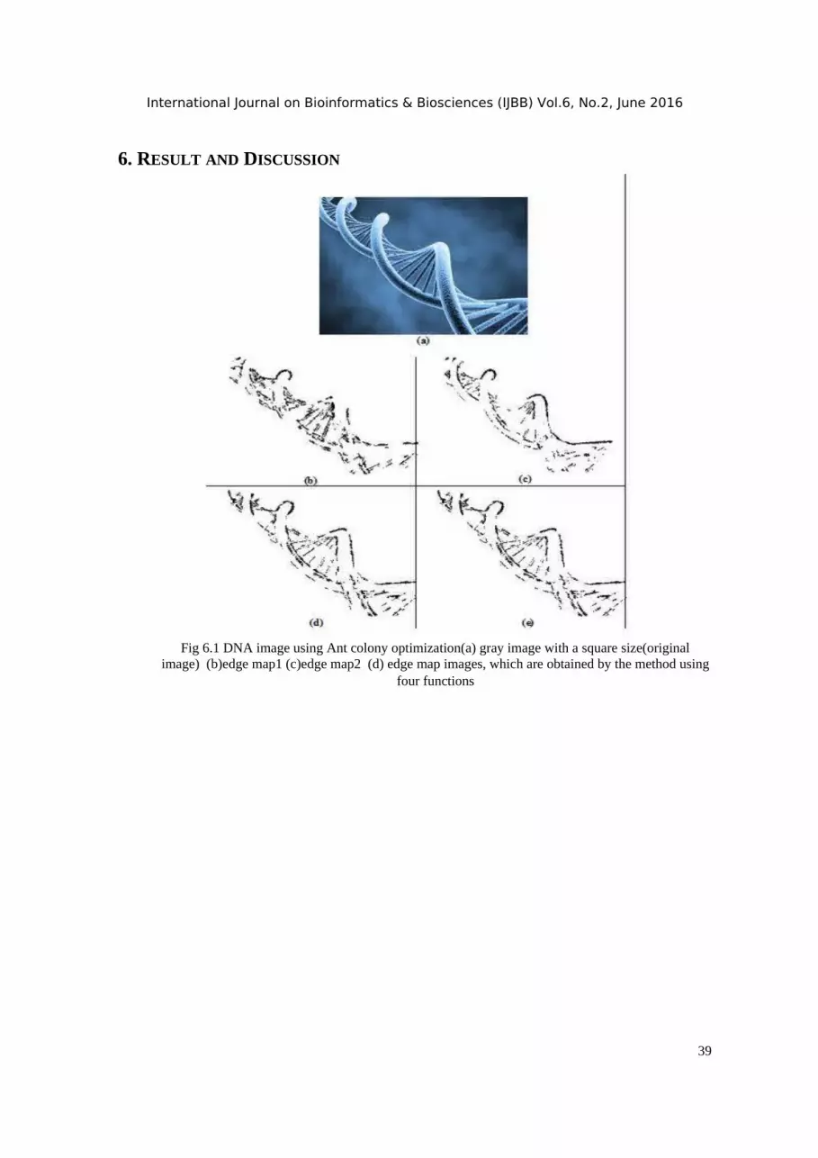
6. RESULT AND DISCUSSION

Fig 6.1 DNA image using Ant colony optimization(a) gray image with a square size(original image) (b)edge map1 (c)edge map2 (d) edge map images, which are obtained by the method using

four functions

39


Fig 6.2 DNA image using Ant colony optimization (a) gray image with a square size(original image) (b)edge map1(c)edge map2 (d) edge map images, which are obtained by the method using four functions

40


Fig 6.3 DNA image using variation Adaptive Ant colony optimization (a)input image (b)output image

7. COMPARISON (using Jaccard)

Table7.1 Comparison of dna images using Jaccard (Ant colony optimization)

41


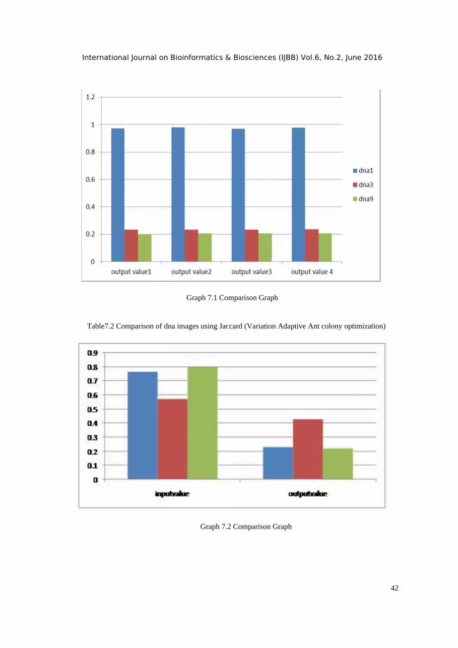
Graph 7.1 Comparison Graph

Table7.2 Comparison of dna images using Jaccard (Variation Adaptive Ant colony optimization)

Graph 7.2 Comparison Graph

42


8. CONCLUSION

In this paper a method for image edge detection using ACO has been used. That the proposed method is successfully developed, it obtained better implementation of existing algorithms edge detection has been proven in the simulation results. Our proposed compared with Jing Tian method for high speed, less processing time and more answers optimum. Also the proposed method has a better edge than other classical methods.

REFERENCES

[1] Agarwal, S., 2012. A Review Paper Of Edge Detection Using Ant Colony Optimization. International Journal of Latest Research in Science and Technology 1, 120–123.

[2] Tian, J., Yu, W., Xie, S., 2008. An Ant Colony Optimization Algorithm For Image Edge Detection, in: IEEE Congress on Evolutionary Computation (CEC). pp. 751–756.

[3] David W. Mount Bioinformatics-Sequence and genomic analysis Cold Spring Harbor Laboratory Press, New York.

[4] Watson, J. D. and Crick, F. H. C. 1953. Molecular structure of nucleic acids: A structure for deoxyribonucleic acids. Nature 171:737–738. 1953.

[5] Bauer, W. R., Crick, F. H. C., and White, J. H. 1980. Super- coiled DNA. Sci Amer. 243:11133.[6] Boles, T. C., White, J. H., and Cozzarelli, N. R. 1990. Structure of supercoiled DNA. J. Mol. Biol.

213:931–951.[7] M. Dorigo, M. Birattari, and T. Stutzle, “Ant colony optimization,” IEEE Computational Intelligence

Magazine, vol. 1, pp. 28–39, Nov.2006.[8] M. Dorigo and T. Stutzle, Ant Colony Optimization , Cambridge: MIT Press, 2004.[9] Gonzalez R.C., Woods R.E. Digital Image Processing, 2nd Ed.. New Jersey, Prentice Hall, (2002).[10] H. Nezamabadi-Pour, S. Saryazdi, and E. Rashedi, “Edge detection using ant algorithms,” Soft

Computing, vol. 10, pp. 623–628, May. 2006.

AUTHORS

Keerthana.S doing M.phil computer science in Gandhigram Rural Institute-Deemed University, Tamil Nadu India and done Master degree in Information Technology in Gandhigram Rural Institute-Deemed University, Tamilnadu India. Her completed B.Sc Information Technology . Her research interest include Bioinformatics and image processing.

43

dna image segmentation – a comparison of edge detection techniques

Documents