A snake for CT image segmentation integrating regionand edge information

X.M. Pardo*, M.J. Carreira, A. Mosquera, D. Cabello

Departamento ElectroÂnica e ComputacioÂn, Universidade de Santiago de Compostela, Campus Sur, 15706 Santiago de Compostela, Spain

Received 2 August 1999; revised 3 October 2000; accepted 5 October 2000

Abstract

The 3D representation and solid modeling of knee bone structures taken from computed tomography (CT) scans are necessary processes in

many medical applications. The construction of the 3D model is generally carried out by stacking the contours obtained from a 2D

segmentation of each CT slice, so the quality of the 3D model strongly depends on the precision of this segmentation process. In this

work we present a deformable contour method for the problem of automatically delineating the external bone (tibia and ®bula) contours from

a set of CT scan images. We have introduced a new region potential term and an edge focusing strategy that diminish the problems that the

classical snake method presents when it is applied to the segmentation of CT images. We introduce knowledge about the location of the

object of interest and knowledge about the behavior of edges in scale space, in order to enhance edge information. We also introduce a region

information aimed at complementing edge information. The novelty in that is that the new region potential does not rely on prior knowledge

about image statistics; the desired features are derived from the segmentation in the previous slice of the 3D sequence. Finally, we show

examples of 3D reconstruction demonstrating the validity of our model. The performance of our method was visually and quantitatively

validated by experts. q 2001 Elsevier Science B.V. All rights reserved.

Keywords: Deformable models; Segmentation; Edge focusing; Region matching; Computed tomography

1. Introduction

Nowadays there is growing interest in the planning and

simulation of medical procedures in order to achieve mini-

mally invasive therapies. To simulate these procedures it is

necessary to create 3D models of the organs of interest. For

instance, the 3D reconstruction of knee bone structures

taken from a set of tomographic cross sections is necessary

in the computer-aided diagnosis of bones' pathologies and

the surgical planning of prosthesis implants and osteotomies

[12,15,23]. The precision of the 3D solid modeling is essen-

tial for the reliable physiological simulation of speci®c

patients' bones. This simulation involves an analysis of

the stress distribution, usually carried out by means of ®nite

elements [5,17,22]. The use of computational techniques

permits repeatability and precision and, as a consequence,

improves the reliability of the extracted clinical informa-

tion.

The main step of geometry reconstruction is segmenta-

tion, in which the tissues of interest (bones) are identi®ed.

CT scans provide cross section images that clearly distin-

guish the dense cortical bone from soft muscle tissues.

However, dif®culties are encountered in deriving the

geometry of the tibia proximal end (close to knee joint);

injuries, bone loss and the bone's inhomogeneous structure

cause the bone to be nearly indistinguishable from soft

tissue. Further, limitations in the resolution of the CT scan

cause the contours of the tibia and the ®bula to combine.

The construction of the 3D model is generally carried out

by stacking the contours obtained from a 2D segmentation

of each CT slice. Manual segmentation has been used to

extract bone geometry, but it is a subjective and tedious

process. There are a number of methods for segmenting

CT images, but, usually, a manual correction has to be

carried out in the bone contouring process. From these

methods, thresholding approaches are the simplest. They

provide binary images composed of regions that identify

objects segregated from the background. Their major draw-

back is the lack of local adaptability; pixels of the same

tissue may exhibit different intensities between slices and

even within the same slice. It is generally necessary to post-

process the image using mathematical morphology [3], and/

or combining thresholding with region growing [37]. Edge-

based methods allow delineation of regions through the

location of their contours as points of high gradient, but

Image and Vision Computing 19 (2001) 461±475

0262-8856/00/$ - see front matter q 2001 Elsevier Science B.V. All rights reserved.

PII: S0262-8856(00)00092-5

www.elsevier.com/locate/imavis

* Corresponding author. Tel.: 134-981-563-100; fax: 134-981-599-412.

E-mail address: pardo@dec.usc.es (X.M. Pardo).

they have a high sensibility to noise, particularly between

regions with small contrast differences, and need gap clos-

ing methods to link edges belonging to the same boundary

[29]. Region-based methods yield parts of the image that

meet the requirements of a given uniformity criterion. One

of the most widely used techniques in this category is region

growing. In its simplest form, the method starts with a small

region and then examines its neighborhood in order to

decide whether or not they have similar features. If they

do, then they are grouped together to form a new greater

region. It has two drawbacks: ®rst, post-processing is

usually required to cope with infra- and over-segmentation,

generally applying domain knowledge [13,33], and second,

it also suffers from bad location of boundaries.

Segmentation of 3D images into 3D regions is similar to

segmentation of 2D images into 2D regions, and the same

kind of methods can be used [30]: thresholding, determina-

tion of boundary surfaces and extraction of volumetric

regions. Results obtained using these classical approaches

are often not satisfactory, because of the unequal scanning

resolution, which causes discontinuity in the input scene, so

restricting direct usage of 3D operations. An interpolation is

usually performed to achieve the same resolution in the

longitudinal dimension as is available in cross sections,

but this generally produces diffuse contours and gray level

discontinuities.

The dif®culty of segmentation is an aspect of global/local

duality. Consideration of local features can lead to over-

segmentation, and erroneous fusions (infra-segmentation)

can be obtained using only global features. To tackle the

problem of obtaining a trade-off between infra/over-

segmentation, (local) edge information and (global) homo-

geneity information must be combined during image

segmentation; region- and edge-based methods are consid-

ered as complementary approaches [10,24,28,36].

Moreover, a meaningful segmentation must take into

account high level descriptions of the objects [9]. A robust

system must be driven both by data and model, and deform-

able model approaches provide a simple and effective way

of doing it [21].

The main goal of this work is to develop an automatic and

robust snake-based approach for 3D segmentation of the

tibia and the ®bula from a set of parallel CT slices. The

method provides repeatable, faster and more objective

results than any manual or semi-automatic contour

delineation.

This work is structured into the following sections: in

Section 2 we describe the characteristics of the images we

will work with, introduce a background theory of snakes and

®nally describe our model. Then, in Section 3, we present

examples of the results obtained with our method, and

®nally, a discussion and the conclusions of the present

work are shown in Section 4.

2. Material and methods

The characteristics of the images we will work with can

be seen in Fig. 1, where we can identify the tibia, ®bula,

cortical bone and trabecular bone. The width and high

density of the cortical bone together with the clear separa-

tion between the tibia and the ®bula (Fig. 1(b)) make the

tibia segmentation in the distal end fairly easy. As we

approach the proximal part of the tibia, the thickness of

the cortical bone decreases and the distance to the ®bula

is reduced. Typically, images of slices with injuries (bone

loss, cortical bone narrowness, malformations, etc.) show

poorly de®ned external bone contours, little separation

between the internal and external contour of the cortical

bone, and incomplete borders between different bones

X.M. Pardo et al. / Image and Vision Computing 19 (2001) 461±475462

Fig. 1. Scheme of low knee bones: (a) cross section close to the proximal end; and (b) cross section close to the distal end.

(tibia and ®bula, tibia and femur). Fig. 1(a) illustrates some

of these problems. In a snake-based approach, the contour

can be trapped by spurious edge points. This makes the ®nal

result very sensitive to the initial conditions. For a correct

delineation of the contour, the ®tting to the external side of

the cortical bone is of paramount importance [25]. When

processing slice sequences, the contour in the previous slice

can be used as the initial deformation state in the present

slice [2], but approximation problems arise when injuries or

deformations appear. Although the classical edge-oriented

deformable contour models have demonstrated high ef®-

ciency in the segmentation of biomedical structures, they

are not free of limitations [20]. In damaged areas of bones or

in the boundary between different bones (tibia and ®bula),

the border information can be incomplete or even be

completely lost. Since the classical snakes are based on

gradient information, they share the limitations of edge

detectors. Ronfard [32] proposed a new deformable model

that uses no edge information, but local computations

around contour neighborhoods (region information). Statis-

tical models of object and background regions are used to

push the model towards border points. Region information

can provide clues to guide the evolution where gradient

information vanishes (homogeneous areas). This method

was proposed for the case of step-edges but can not distin-

guish boundaries between objects of similar features. Ivins

and Porril [14] proposed a related approach where a snake is

driven by a pressure force that is a function of the statistical

characteristics of image data. The model expands until it

®nds pixels that lie outside user-de®ned limits relative to

the statistical characteristics of a seed region; when these

limits are crossed the pressure force is reversed to make the

model contract.

Region features present the advantage of being less sensi-

tive to noise. Their inconveniences reside in that the change

of the pixel characteristics that suggest the presence of a

contour remains diluted in the global character of the region

features. This frequently provokes the undesired merging of

regions. This problem can be alleviated with gradient/edge

information. Chakraborty et al. [8] proposed a deformable

boundary ®nding approach that integrates region and edge

information for the segmentation of homogeneous struc-

tures surrounded by a single background. This approach

must know a priori which regions belong to the object of

interest. This idea is extended to 3D in Ref. [34].

A unifying framework that generalizes the deformable

model, region growing and prior matching approaches was

proposed by Zhu et al.[38]. The method combines local and

global information, and local and global optimization. It can

be applied both for obtaining global segmentation of images

and ®nding individual regions. However, the ®nal solution

does not consider shape information.

Most of the above approaches use prior models for their

region-based statistics, which limits usefulness in situations

where a comprehensive set of priors is not available. In case

of bone segmentation the object of interest is a heteroge-

neous structure (bone) made of different tissues with differ-

ent texture features, and we do not know a priori the

statistics of all the tissues that belong to the bone. Some

of the bone tissues appear in a CT image with texture

features similar to soft tissues; cortical bone statistics

change from slice to slice (due to bone loss, injuries, etc.),

different bones (tibia and ®bula, for instance) have similar

statistics, etc. So region information must be used in a

different way. In this work we present a new deformable

contour approach that uses an approximated initial model

and combines region and edge information in a cooperative

way to solve the problems of delineating the external side of

the cortical bone of the tibia and the ®bula from CT scan

images. We introduce knowledge about the location of the

object of interest and knowledge about the behavior of

edges in scale space in order to enhance edge information.

We also introduce a region information aimed at comple-

menting edge information that does not rely on prior knowl-

edge about image statistics; the desired features are derived

from the segmentation in the previous slice.

2.1. Classical deformable contours

A snake [16] is an elastic curve that, located over an

image, evolves from its initial shape and position as a result

of the combined action of external and internal forces. The

external forces lead the snake towards features of the image,

whereas internal forces model the elasticity of the curve. In

a parametric representation, the snake appears as a curve

u�s� � �x�s�; y�s��; s [ �0; 1�; with u�0� � u�1�: Its internal

energy is often de®ned as

Eint�u� �Z1

0�auus�s�u2 1 buuss�s�u2�ds:

It is made up of two factors: the membrane energy

auus�s�u2; which weights its resistance to stretching, and

the thin-plate energy, buuss�s�u2; that weights its resistance

to bending. us(s) and uss(s) represent the ®rst and second

derivatives, respectively. The elasticity parameters a and

b control the smoothness of the curve.

The external energy is generally de®ned as a potential

®eld P,

Eext�u� �Z1

0P�u�s�� ds:

Typical terms in the expression of the external energy are

[11,31]:

PI � ^gI�u�s��; �1�where I is the intensity image, and attracts the curve to high

or low intensity points;

PG � 2zu7�Gs�u�s�� p I�u�s���u; �2�where Gs represents a Gaussian ®lter with a scale parameter

s , and attracts the curve to intensity edges, after

X.M. Pardo et al. / Image and Vision Computing 19 (2001) 461±475 463

convolution with a Gaussian smoothing; and

PE � 2he2d�u�s��2; �3�

where d(u(s)) is the distance to the closest boundary point,

which pushes the contour to the edge points belonging to a

contour image in which edges are detected by means of an

edge detector ®lter.

Parameters g , z , h in Eqs. (1)±(3) are positive constants

that weight the contributions of the different terms in the

external energy. The total energy of the snake will be the

sum of the external and internal energies along the curve

u(s):

Esnake � Eint�u�1 Eext�u�:The solution to the problem of detecting the contour is

found in the minimization of this energy function. In order

to numerically compute a minimal energy solution it is

necessary to discretize the expression of the energy. So

from the curve u(s) a set of N control points, vi � �xi; yi�; i �1;¼;N; is chosen. The selection of these points can be

carried out so that they are evenly spaced in the parameter,

s, of the curve (u�s� ! vi; i � 1;¼;N; so that uvi 2 vi11u �Ds�; so Ds £ N equals the size of the curve u(s).

2.2. A snake model for CT image segmentation

Classical potentials do not hold enough information to

tackle the bone segmentation in CT images. In order to

endow the snake with enough ability to manage this

problem, we have introduced new external energy terms.

The external energy is chosen to combine region and gradi-

ent/edge information in order to make the whole procedure

more robust to noise, low contrast and bad initialization. We

will use the two classical potential terms PI and PG

described in Eqs. (1) and (2), and two more, PR and PE0:

PR will introduce region information and PE0 will modify PE

in Eq. (3), considering directional derivative information.

Moreover, we have introduced an edge focusing process

in the generation of the edge map used to calculate PE0: In

this way we substantially reduce the number of inadequate

snake attractors (noisy and weak edges). In the following

subsections the computation of each new potential term is

explained.

2.2.1. Edge external energy �PE0�

Edge information, used to compute the edge potential, is

usually obtained using a single scale edge detector without

any constraint in edge location. However, this information

can be enhanced. On the one hand, features of the same

object appear at different scales, therefore each part of the

image needs to be ®ltered in a different way and an optimal

single scale does not exist. So we will obtain the edge map

by combining the outputs of the edge detector using differ-

ent scales. On the other hand, it does not distinguish among

edges belonging to different objects, so undesired snake

attractors can be generated. We will use knowledge about

the location of the edges of interest. In this way, we will

retain only edges belonging to the object of interest and thus

the edge information will be more valuable for deriving the

edge potential.

Next, we will describe the procedure to select edge infor-

mation (edge map focusing) and the modi®ed edge poten-

tial.

Edge map focusing. To obtain the edge map, a Laplacian

of the Gaussian (LoG) ®ltering [19] is applied to the original

image,

LoG�x; y;s� � 7 2�G�x; y;s� p I�x; y��:So, edge locations correspond to zero-crossings in the

®ltered image and each edge point is characterized by its

intensity gradient. The LoG ®lter combines a smoothing

process with the detection of intensity changes to make

the detection less sensitive to noise. Multiscale edge detec-

tion has been proposed to detect edges at several spatial

scales [7,19]. We will try to integrate all this information

taking into account both knowledge about the behavior of

edges in scale space [18] and a priori knowledge about the

domain. Fig. 2 shows the block diagram of the strategy

proposed to detect salient edges in the image. First we detect

the zero-crossings of the LoG ®lter using different scales,

then we perform a focusing on salient edges over each scale

image using a set of constraints and, ®nally, we integrate

information from all scale focused images to provide the

salient edges image.

The edge detector block performs the extraction of edges

X.M. Pardo et al. / Image and Vision Computing 19 (2001) 461±475464

Fig. 2. Edge focusing scheme: The Edge detector block provides a set of

edge images after obtaining zero-crossing of the LoG ®lter with different

scales. The Focusing block retains the salient edges for each of the afore-

mentioned images. The Analysis in scale space block provides a unique

edge image after integrating information from different scales.

at different scales, providing edge images Iis1;¼; Iisn

for

each slice i. It is necessary to choose the scale parameter

sequence {s1;¼;sn}; �s1 . ¼ . sn�; that veri®es the

following constraints [18]:

² each edge curve of interest must exist in Iis1;

² Iis1must contain few irrelevant zero crossing curves;

² {Iis1; Iis2

;¼; Iisn} should provide enough information to

recover the accurate shape and location of the curve of

interest;

² n must be the minimum integer that meets the require-

ments of the aforementioned conditions.

The number n and values s j of scale parameters are

chosen so that neither loses any important edges and so

that noisy details do not remain. If the maximum scale para-

meter is too large, some signi®cant edges may get lost; if it

is too small, too many details and noise will be generated

[4]. We have chosen three values {s1 � 1; s2 � 2; s3 �3} as a compromise between these two facts.

The Focusing and Analysis blocks of Fig. 2 tackle the

problem of retaining only salient edges, using knowledge

about the domain and knowledge about the behavior of

edges in scale space. Both are represented as a set of f

constraints. In this way we will transform, for each slice i

and each scale s j, its initial edge map Iis jinto a ®nal edge

map Ifis j

satisfying all the f constraints, where Ikis j

is the edge

map in slice i, with scale s j, after applying the k ®rst

constraints, and I0is j� Iis j

is the initial edge map.

The ®rst constraints, embodied in the Focusing block of

Fig. 2, reduce the number of edges by tempering the effect

of noise, ®ne details and trabecular structure. The inputs to

this block, for slice i, are the edge maps Iis jcorresponding to

each scale s j of the ®lter, and the outputs are the salient edge

maps Ifis j; as shown in Fig. 2.

We will describe the focusing process for a slice i

and a scales j, Iis jcoming from the edge detector block of Fig.

2. The transformation carried out by the Focusing block is]

made up of a set of operations (projections). For each

constraint k, we de®ne a projection operator Pk, which

transforms the contour map Ik21is j

to the nearest map Ikis j

satisfying the corresponding constraint k.

The ®rst projection operator P1 performs the amplitude

constraint discarding noisy edges and edges due to weak

transitions in the following way:

I1is j�x; y� � P1�I0

is j�x; y�� �

1 : I0is j�x; y� . tg

0 : I0is j�x; y� # tg

8<: �4�

where tg represents a gradient threshold. A value could be

given to tg following different criteria: a heuristically

derived constant, a percentage of maximum gradient value

or a value related with the average value on the previous

slice ®nal contour. When the original image sequence is

completed with interpolated slices (to increase the longi-

tudinal resolution of volume data) we found that the second

method is the best.

A support constraint is introduced to take advantage of

the small distance between slices from which the ®nal

contour segmentation obtained in the previous slice should

be a good approximation to I2is j: This constraint integrates

knowledge about the location of the contour. We have

implemented this constraint through three projection func-

tions P2, P3 and P4, as follows:

I2is j�x; y� � P2�I1

is j�x; y��

�1 : I1

isj�x; y� � 1 AND iI1

isj�x; y�2 I

f�i21�s j

�x; y�i # ts

0 : I1is j�x; y� � 0

0:5 : otherwise

8>>><>>>:�5�

I3is j�x; y� � P3�I2

is j�x; y��

�1 : I2

is j�x; y� � 1

1 : I2is j�x; y� � 0:5 AND I2

is j�x 1 dx; y 1 dy� � 1

0 : otherwise

8>>><>>>:�6�

I4is j�x; y� � P4�I3

is j�x; y�� � 1 : I3

is j�x; y� � 1

0 : otherwise

(�7�

with dx, dy [ {0; 1}: P2 tries to retain edges close to the

®nal contour of the previous slice, introducing the inter-slice

distance by means of the parameter ts. The greater the inter-

slice distance, the greater the value of ts. If an edge point is

not close to an edge point in the previous slice, it is not

eliminated. The goal of P3 is to recover full edge segments

that have some edge points close to the approximated

previous contour. Little offsets are applied to each point

(x,y) in order to ®nd edges close by. They are iteratively

applied until no changes occur in edge estimation. In this

way, an edge point with value 0.5 can get value 1 if it

belongs to an edge segment having some points with this

value. Finally, operator P4 eliminates spurious edge points

(value 0.5 in I3is j� that are distant from the model. So P4

discards edge points belonging to edge segments that do

not have correspondence in the previous slice. In this way,

a ®nal image Ifis j

is obtained as f � 4 in our case.

We could think about joining P3 and P4, but the iterative

nature of P3 requires a separated process. To merge the two

projectors in a single one the operation should be edge-

segment based, not edge-point based as we have implemen-

ted it.

The image set Ifis1

;¼; Ifisn

is the input to the Analysis

block of Fig. 2, where the integration of information in

scale space, for slice i, is implemented. This integration

leads to the unique edge map Ifi : We have followed an

integration scheme based on the knowledge of edge

X.M. Pardo et al. / Image and Vision Computing 19 (2001) 461±475 465

behavior in scale space [18], starting with the location of

edge points obtained with a large scale and re®ning their

location using information from lower scales. The system

starts by considering the two highest scales and applies a set

of procedures for correcting edge locations (CEL), recover-

ing missing edges (RME), and removing noise and false

edges (RNFE). The CEL procedure searches, for each

edge in the highest scale, its nearest one in the lowest

scale. The RME procedure recovers, in the lowest scale,

edge segments that do not correspond to the highest scale

but are connected to edges remaining after CEL. We have

not applied the RNFE procedure because it can end up

removing edges of interest. The resulting edge map is

again combined with the one obtained in the next scale.

The process ®nishes after integrating the information of

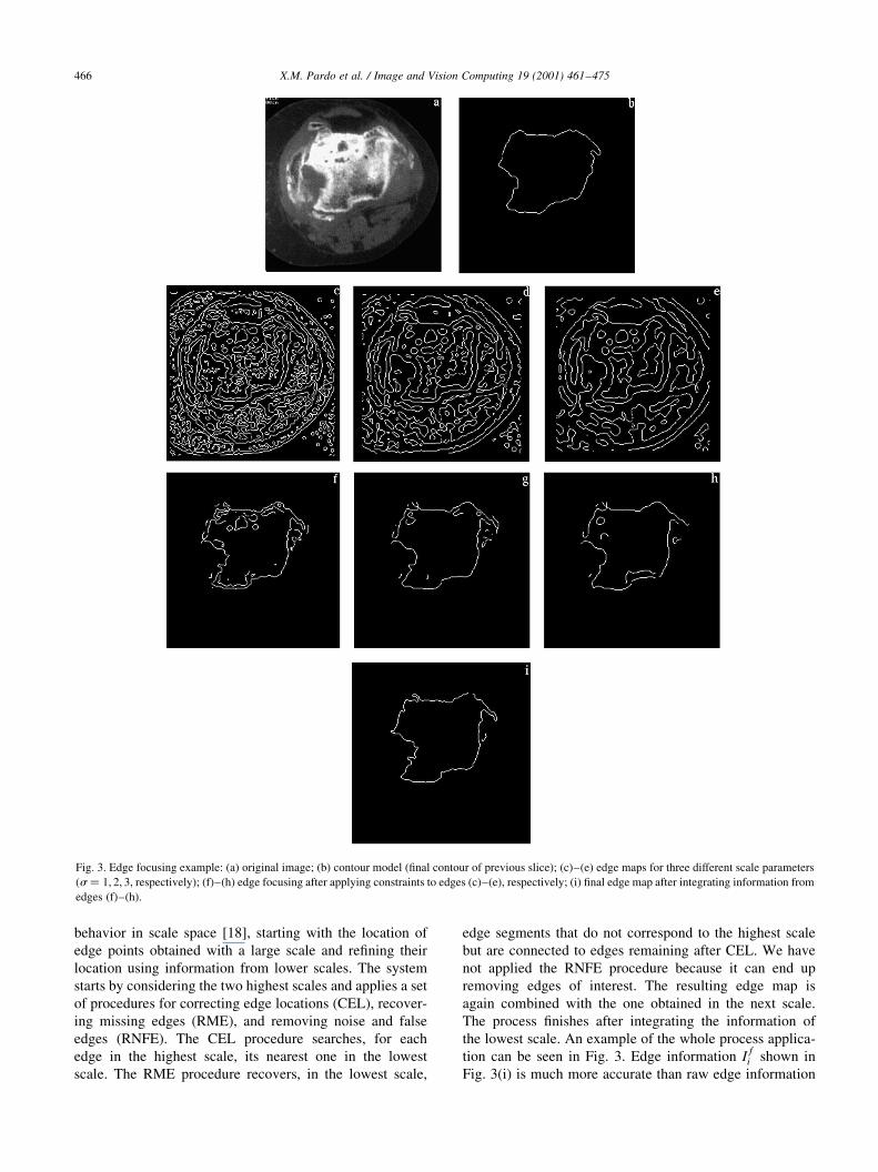
the lowest scale. An example of the whole process applica-

tion can be seen in Fig. 3. Edge information Ifi shown in

Fig. 3(i) is much more accurate than raw edge information

X.M. Pardo et al. / Image and Vision Computing 19 (2001) 461±475466

Fig. 3. Edge focusing example: (a) original image; (b) contour model (®nal contour of previous slice); (c)±(e) edge maps for three different scale parameters

(s � 1; 2; 3; respectively); (f)±(h) edge focusing after applying constraints to edges (c)±(e), respectively; (i) ®nal edge map after integrating information from

edges (f)±(h).

�Iis1; Iis2

; Iis3� in Fig. 3(c)±(e) and �I f

is1; I

fis2

; Ifis3� Fig. 3(f)±

(h). From this edge map we can derive an edge potential as

in Eq. (3). However, a more convenient external energy can

be obtained as will be set out below.

Modi®ed the edge potential, PE0: One of the problems in

deformable contour methods that must be addressed is the

bad initialization, which could cause the snake to fall into a

local minimum. When trying to determine the external

contour of a bone, these problems occur if the initial contour

is positioned inside the cortical bone, or when this contour is

located between two different bones (for instance, the tibia

and the ®bula). In those cases, the classical edge potential PE

does not discriminate between internal and external

contours.

To mitigate problems of bad initialization, the use of

directional information in snakes have been independently

proposed by different authors [25,31,35]. In Ref. [25] we

have proposed an external energy term to distinguish

between internal and external contours of any bone structure

as well as to locate the desired bone boundary even in the

case of con¯icting structures located close to the desired

bone. Its expression for a vertex vi is as follows:

P 0E�vi� � he2d�v�i��2 ´min 0;2

2~nI�vi�

� �; �8�

where ~n represents the direction normal to the snake and

d(v(i)) is the distance to the closest boundary point, as in Eq.

(3). When the structure has double contours, this new energy

term presents the minimum value in the exact position of the

external contour seen from the curve's mass centre

(centroid). When the initial model is located between two

close structures, for example the tibia and the ®bula, this

potential term attracts the curve towards the contour that is

closest to the centroid of the snake. The curve is attracted

towards the external contour of the tibia if the initial model

corresponds to the contour of the tibia in the previous slice,

and towards the external contour of the ®bula if the initial

model corresponds to the ®bula in the previous slice.

We take min{0; �2=2~n�I�vi�} to avoid undesired bound-

aries preventing the snake from evolving towards the

features of interest. While PE (see Eq. (3)) is a constant

potential image, PE0 sees edges in a different way depending

on the direction of the normal to each snake's vertex.

2.2.2. Region energy, PR

As formerly, edge-detection and region-growing techni-

ques can be used together to produce more accurate and

repeatable segmentation. Primitive methods use only local

properties of pixels to grow regions. More sophisticated

techniques grow regions by merging smaller subregions.

The effectiveness of region-growing algorithms depends

on the application. If the image is simple enough the local

techniques can be very effective. However, on complicated

images even the most sophisticated techniques may not

produce a useful segmentation. In this case, region growing

is sometimes used together with more knowledgeable

processes [26].

In this approach, the region information arises from a low

level region-based segmentation where each pixel in the

image is classi®ed into one of a number of classes. From

all the approaches to region-based segmentation, we have

performed the region segmentation of CT knee images using

a self-organizing feature map [6]. This Kohonen neural

network carries out a competitive learning process that clas-

si®es the image pixels into different tissue types. The train-

ing involves modifying the weighting vector for each output

node that is marked for a given input. The label associated to

each node is its position in the array of output nodes. Each

step in the learning process updates all weight vectors in the

neighborhood of the winning output node, so neighboring

nodes learn close bone patterns. This characteristic and the

fact that we use one feature (density) and a 1D topology of

the neural network guarantee the ordering of labels. In this

way, when the label value increases, we go from soft to hard

tissues or vice versa, but always keeping the ordering in

density. Since the bone is an heterogeneous structure

made up of several tissues, and some bone tissues could

have texture features similar to soft tissues (muscle), the

low level classi®cation produces an over-segmentation.

However, this over-segmentation brings additional informa-

tion to the snake model: ®rstly, it is able to guide the direc-

tion of snake evolution in homogeneous parts where edge/

gradient vanishes, and secondly, it makes the snake deline-

ate the bone taking into account texture features of internal

and external regions. We will show an example of region

segmentation later.

To obtain the region potential we proceed in the follow-

ing way. First, for each region border point in the previous

slice, pi21, we look for the corresponding region border

point in the actual slice pi. It must be noted that the matching

is established between regions, so the snake contour will be

pushed towards the region border. Depending on the side of

the region ®tted by the snake, the region will be inside or

outside the contour. To move the contour to the correct side

we introduce an orientation term in the region potential PR.

The matching of border points in slice i, pi, is found in the

minimum of the following cost function:

M�pi; pi21� � w1 £ �L�pi�2 L�pi21��1 w2 £ �u�pi�2 u�pi21��1 w3 £ d�pi; pi21�; �9�

where L and u are the region label and the orientation of a

boundary point, respectively, d is the distance between

border points in previous and actual slices, and w1, w2 and

w3 are the weights of each term and take values 0.5, 1.0 and

0.1, respectively. The ®rst term measures distances in label

values, which is equivalent to measuring distances between

densitometric features of regions. The second term

measures the deviation between border orientations; it

works to do the matching between the same part of the

two regions. It characterizes border points by their

X.M. Pardo et al. / Image and Vision Computing 19 (2001) 461±475 467

orientation, allows discriminating between border points of

the same region, and between border points of neighboring

regions of the same or different classes. Finally, the third

term measures distance in locations.

The matching point p̂i in the actual slice for the border

point pi21 in the previous slice will be:

p̂i � arg minpi

M�pi; pi21�: �10�

It is necessary to emphasize that the difference in orienta-

tion between corresponding border points must be less than

58 to avoid matching between very different orientations.

When processing a temporal or spatial sequence, it is

possible to reduce the computational cost of this matching

by working only in a small neighborhood of the contour

delineated in the previous slice.

From the matching between regions around the contour in

slice i 2 1 and regions in slice i, we obtain a signed offset in

x and y coordinates (Dx,Dy), from each point pi21 in slice

i 2 1 to the region matched point p̂i in slice i. To eliminate

erroneous matchings between regions of the two slices we

perform a median ®ltering of these offsets along the contour.

By adding the ®ltered offsets to each contour point pi21 in

slice i 2 1, we obtain the matching contour (MC) in slice i.

Finally, the region potential is obtained computing the

distance from each image point to the MC.

Sumarizing, for each point in the external contour of the

bone in slice i 2 1 we look for points in slice i with similar

region features. If vi is a snake vertex, we will express its

region potential as:

PR�vi� � kd�vi;MC�; �11�where k is a positive constant and d(vi,MC) represents the

distance from point vi to the nearest point in MC. In our

experiments d is the Euclidean distance. This potential

(linear function of distance) is not as steep as the edge

energy P 0E (negative exponential function of squared

distance, Eq. (8)) when the Euclidean distance approaches

zero, but it is steeper when the distance is large. In this way,

the region potential guides the snake evolution within the

homogeneous areas, and the edge potential takes the control

in the proximity of edge points because of its better accu-

racy in the location of border points. In this way we try to

avoid the accumulation of errors in the following way:

region information pushes the contour from homogeneous

areas (interior of regions) towards the border between

regions, then the edge information becomes more important

and looks for the external contour of the bone as demon-

strated in Ref. [25]. The region potential is adequate for

large displacements and the edge information is better for

local ®tting of the contour.

Synthetic images in Fig. 4 illustrate the effect of this region

energy. Fig. 4(a) and (b) represent two images in a temporal or

spatial sequence. Let us suppose that the biggest circle has

already been segmented in Fig. 4(a) and now, we are interested

in segmenting the same circle in Fig. 4(b). Fig. 4(c) shows the

X.M. Pardo et al. / Image and Vision Computing 19 (2001) 461±475468

Fig. 4. Example of the evolution of the curve guided by region energy: (a) and (b) adjacent slices in a sequence; (c) ®nal delineated contour in image (a) over

image (b); (d) ®nal contour for image (b).

®nal contour for the biggest circle in Fig. 4(a) (actual initial

contour) superposed on the image in Fig. 4(b). Thus, the initial

contour encloses part of the smallest circle. However, the

region potential is able to distinguish between the nearest

contour of the smallest circle and the true corresponding

contour of the biggest circle. Fig. 4(d) shows the ®nal contour

after deformation by only taking into account the region poten-

tial.

Fig. 5 illustrates all the processes in computing the region

potential and establishes some comparisons with edge infor-

mation. Fig. 5(a) shows the original image and Fig. 5(b)

contains the edge information after focusing edges. As can

be seen, edge information only permits a local adjustment

but contains some ambiguities because it does not permit to

distinguish between bone contour and leg contour.

However, it must be noted that the edge potential will be

able to distinguish between internal and external bone

contours, but not between external bone contour and exter-

nal edge contour. Later, in Fig. 8 we will illustrate this fact.

Fig. 5(c) and (d) contains the region segmentation obtained

for the previous slice and the actual slice, respectively. Each

region is identi®ed by its label that is ordered by tissue

density as aforementioned. Fig. 5(e) shows the matching

between the regions around the contour in the previous

slice with region borders in the actual slice and, ®nally,

Fig. 5(f) shows the region potential PR obtained after ®lter-

ing the matching contour and computing distances.

2.3. Energy minimization

After introducing the new methodology and potential

terms, the full expression for the external energy is:

Eext�vi� � PG 1 PI 1 P 0E 1 PR

� 2gu7�G�vi� p I�vi��u 2 dI�vi�

1 he2d�v�i��2 ´min 0;2

2~nI�vi�

� �1 kd�vi;MC�; �12�

where d(vi) denotes the distance between vertex vi and the

closest edge in the previously obtained edge map, as

described in Section 2.2.1, and g , d , h , k are positive

constants. The intensity and the gradient are useful for guid-

ing the snake in areas where edge information is lost. These

®rst three terms take values between 0 and 255. The region

potential takes values that depend on the accuracy of the

initial contour, but are much smaller than the other terms.

We determine heuristically the weights g � 1; d � 1; h �4; k < 50: These weights have been set to normalize all the

potential terms in order to obtain a similar contribution from

all of them. After processing several sequences of CT

images, we found that, on average, all the terms have the

same signi®cance.

The external energy is combined with the classical inter-

nal energy:

Eint�vi� � ai�vi 2 vi21�2 1 bi�vi21 2 2vi 1 vi11�2; �13�to obtain the total snake energy. a and b take small values

( < 0.01). In fact, they can have value zero if the contour is

represented by means of B-splines (smooth shapes).

The solution to the problem of detection of the outer

contour is given by the minimization of the sum of energy

functions in Eqs. (12) and (13) over all the snake vertices. In

our case, the initial external contour is the contour obtained

from the segmentation of the previous slice in the sequence.

This fact allows a constrained search of the energy mini-

mum along the direction normal to each contour vertex. We

have used a method based on dynamic programming [1]

where an oriented segment of the possible displacement is

de®ned for each vertex of the snake. Each segment is

oriented in the normal direction to the curve and centered

on a vertex. In this way computation is 10 times lower than

having to explore all the neighborhood, and the solution

does not get worse [25]. One of the main advantages of

dynamic programming is that it does not require the energy

functional to be differentiable, so it can be used to impose

X.M. Pardo et al. / Image and Vision Computing 19 (2001) 461±475 469

Fig. 5. (a) Original slice in a CT image sequence; (b) edge map after edge

focusing; (c) region segmentation of the previous slice in the sequence; (d)

region segmentation of the current slice (a); (e) matching contour; (f) region

potential.

hard constraints on the model and to employ energy terms

where a variational principle is dif®cult to derive.

Given three consecutive control points (vertices)

vk; vk11; vk12; the vertex vk11 can only be moved along a

segment centered on itself and normal to the straight line

connecting vk and vk12 (see Fig. 6). Then, starting from an

initially ®xed arbitrary vertex, dynamic programming was

used to determine the position of the remaining contour

control points for the energy minimum. The starting vertex

changes in each iteration of the algorithm, thus the

constraint of going through the ®xed initial and ®nal points

is eliminated. The process is repeated until a global mini-

mum of the snake energy is achieved. In each iteration the

segment of the control points' variation is recalculated to

make the shape of the snake ¯exible. This segment is deter-

mined from the normal to the curve for the external contour

of the cortical bone, and parallel to the horizontal axis for

the internal contour.

3. Results

When an initial approximated contour can be provided,

for example when segmenting sequences of CT slice

images, the object can be roughly determined. By means

of a deformable contour that integrates region and edge

information the spatial location of the object boundary can

be precisely de®ned.

Experiments were carried out with different sets of CT

knee images to verify the performance of the system. Fig. 7

corresponds to a case where an injury appears between the

tibia and the ®bula. These two bones are very close as can be

seen in Fig. 7(a), where the initial contour is superposed.

Fig. 7(b) shows the poor result obtained using the classical

energy terms, where PE was calculated from an edge map

obtained using a single scale edge detector. The classical

edge/gradient potentials are not able to distinguish between

external and internal contours of the cortical bone, or

between the tibia and the ®bula. It only looks for the nearest

raw local edges and the high gradient points. Fig. 7(c) shows

the ®nal ®tness reached using the combined action of clas-

sical terms with edge focusing and directional derivative

potential integrated in P 0E: The result improves, but tibia

edge points trap part of the external contour of the ®bula

X.M. Pardo et al. / Image and Vision Computing 19 (2001) 461±475470

Fig. 6. Searching area for the energy minimum. The solid curve represents

the initial contour and the dotted curves enclose the area where the mini-

mum is searched. Segments normal to the curve represent the permitted

displacement of each snake vertex.

Fig. 7. (a) Original image with an injury between the tibia and the ®bula with the initial contour superposed; (b) segmentation obtained using classical energy

terms; (c) delineation of external bone contours obtained by adding a directional derivative energy term; and (d) improved results after integrating region and

edge/gradient information.

due to the fact that the initial ®bula contour is inside the

tibia. In this case, a good delineation of the tibia and

the ®bula can not just rely on edge/gradient information.

The region information derived from a region-based

segmentation pushes the snakes out of the confusing area,

and the edge information ®ts the snakes to the external

contours of the tibia and the ®bula. Thus, the result improves

integrating region and edge/gradient features, as shown in

Fig. 7(d).

Fig. 8 shows an example that belongs to a different image

sequence, where problems arising from bone loss and

narrow cortical bone are present. Fig. 8(a) shows the loca-

tion of the initial contour (®nal contour of the previous

slice). It can be observed that the initial contour is partially

located inside the tibia and other part is located outside the

tibia between the tibia external contour and the knee

contour. Fig. 8(b) represents the ®nal delineation obtained

by classical gradient and edge potentials, where the contour

is pushed towards the nearest edges and local gradient

maxima. Exchanging the classical edge potential PE for

the new edge potential P 0E the result improves, as can be

seen in Fig. 8(c). At this moment, a lot of spurious edge

points are discarded, although several of them remain. Fig.

8(d) illustrates the global effect of the new edge and region

potentials, where it is possible to distinguish between the

tibia contour and the knee contour, and between trabecular

edges and external cortical bone. Region energy is not

enough because of the well known problem of non-optimal

contour location of region segmentation. Moreover, due to

the low contrast in this slice, some bone and muscle zones

X.M. Pardo et al. / Image and Vision Computing 19 (2001) 461±475 471

Fig. 8. (a) Original image with initial contour location; (b) segmentation

obtained using classical energy terms; (c) delineation of external bone

contours obtained with the new edge potential; and (d) improved results

after integrating the new region and edge information.

Fig. 9. (a) Original image with a high density injury; (b) edge map; (c) ®nal contour using only gradient and edge information; and (d) ®nal contour when

adding region information to (c).

appear merged in the aforementioned pre-segmentations

from which region potentials are computed.

Fig. 9 illustrates a case with very low contrast and signal

to noise ratio. After the edge focusing process (Fig. 9(b)),

edge information is not detected in the left, near the location

where the external contour was detected in the previous

slice. This is due to the low quality of the cortical bone in

this part. Actually, a strong contour is located around a high

density injury inside the bone. Although it is dif®cult to see,

the injury is inside the trabecular bone and the real external

contour of the bone is not around the brighter part (injury).

The edge focusing process does not extract edge points in

some parts of this area because the contour that supplies

location constraints (®nal contour in the previous slice) is

more on the right, real edge points in the current slice are

very weak (low gradient) and the injury contour is far from

the model contour used in edge focusing. Fig. 9(c) shows the

result (better than the result obtained with classical snake

implementations) only considering gradient and edge infor-

mation, as described in Ref. [25]. The gradient and direc-

tional derivative potentials push the snake towards the

injury edge points. Part of the contour is correctly ®tted

but, in the area indicated by the arrow, these energy terms

push the snake towards the injury and deviate it from the

external cortical bone. In that case the cortical bone has very

low density, which was the cause of the fracture that

provoked the lesion. The injury is brighter because part of

the bone of the tibia plateau embedded itself in the trabe-

cular bone. Fig. 9(d) shows the improved ®nal contour after

the integration of region and edge features. It can be seen

how region information allows the improvement of the

delineation of the tibia external contour.

Fig. 10 shows the surface reconstruction from the 2D

contours obtained after segmenting a CT image sequence.

This ®gure corresponds to the proximal end of the tibia and

the ®bula of a patient. We use the free software packages

Nuages and Geomview for the triangulation of contours and

visualization of the surface, respectively.

To evaluate objectively the importance of including edge

focusing, directional derivatives and region information, we

considered two real images where a correct segmentation is

provided by our approach. Then Gaussian noise was added

and contrast reduced. To characterize the segmentation

quality we applied the judging criteria used in Ref. [36].

X.M. Pardo et al. / Image and Vision Computing 19 (2001) 461±475472

Fig. 10. Example of a 3D reconstruction after segmenting a CT image

sequence.

Fig. 11. (a) Original image; (b) two intermediate images with decreasing contrasts; and (c) same original image with two increasing levels of added Gaussian

noise.

Let Rf denote the feature value obtained from a reference

image and Sf denote the feature value measured from the

segmented image. The performance criterion, which is

called Relative Ultimate Measurement Accuracy of an

object feature (RUMAf), is computed by:

RUMAf � 100uRf 2 Sf u

Rf

: �14�

The smaller the value of RUMAf, the better the quality of

the segmentation. In our case, features Rf and Sf are the set of

pixels belonging to the objects of interest, computed from

the binary segmentations. Rf will be the set provided by

manual segmentation on the original image (ground truth

segmentation), and Sf will be the set provided by our

approach in images with an added noise or reduced contrast.

uRf 2 Rsu counts the number of pixels that differ between the

two segmentations. So RUMAf measures the percentage of

overlapping between the two segmentations.

To carry out the experiment we considered an original

image with a well de®ned cortical bone, and then we gener-

ated two sequences of six images: one sequence with a

decreasing contrast, and the other with an increasing Gaus-

sian noise. We obtained the segmentations with and without

region information and compared them with the correct

segmentation obtained for the original image (ground

truth). Fig. 11(a) shows the original image, Fig. 11(b) illus-

trates two intermediate images with decreasing contrast, and

Fig. 11(c) shows the original image with two increasing

levels of added Gaussian noise. The segmentations of

these images were obtained when using only edge/gradient

information and when region information was also consid-

ered. As we expected, the performance of both methods is

worst when noise is increased and contrast is decreased. But

the integrated method performed better than the method

without region information.

We then took the manual segmentation of the original

image as the real segmentation and computed the value of

RUMA in three cases: using only classical terms, including

edge focusing and directional derivative potential, and

adding region potential. Fig. 12 shows the graphical repre-

sentation of this error measure. In this way an objective

comparison of quality is presented that con®rms the visual

subjective valuation. The new approach clearly improves

the classical implementation performance. When the

image degradation increases, the region information

becomes more valuable. Initially, region information does

not improve segmentation because the cortical bone is

perfectly de®ned and the edge/gradient information

achieves good results. When the cortical bone quality get

worst, edge/gradient information becomes imprecise and

region information begins to be important.

X.M. Pardo et al. / Image and Vision Computing 19 (2001) 461±475 473

Fig. 12. Comparison between segmentations obtained using classical terms, adding edge focusing and directional derivative potential, and adding region

potential. Original images correspond to the sequences in Fig. 11. The comparison is established in terms of the RUMA between real segmentation and the

segmentations obtained in two cases: when contrast decreases and when noise increases.

Table 1

Comparison with manual segmentations: the ®rst column identi®es the

image, the second one contains the minimal error between the segmentation

provided by the system and the manual segmentations, the third column

shows the error between the automatic segmentation and the average

manual segmentation, and the last column contains the error between the

two manual segmentations

Image

sequence-

number

Minimal

error

(RUMA)

Average

error

(RUMA)

Mutual error

(RUMA)

Seq1-1 1.43 1.53 1.30

Seq1-2 1.54 2.01 2.33

Seq1-3 1.98 2.10 2.87

Seq2-1 3.51 3.52 3.67

Seq2-2 2.13 2.09 2.28

Seq2-3 3.87 3.52 3.04

Seq3-1 3.22 2.99 2.42

Seq3-2 2.37 2.68 2.98

Seq3-3 2.92 2.83 3.42

Seq3-4 2.52 2.97 3.87

We have also compared the results obtained by expert

manual tracing of the contours with the ones achieved by

our method. We have chosen 10 images from three CT

image sequences with different levels of noise and contrast.

For each CT sequence we took images in the proximal,

distal and intermediate part of the tibia and the ®bula.

These images were manually segmented by two experts,

and then using our method. After obtaining the segmenta-

tions the error measure (RUMA) was calculated between:

(1) each one of the hand-traced segmentations and the auto-

mated one, (2) hand-traced segmentations, and (3) average

hand-traced segmentation and the automated one. In Table 1,

the error measures are shown for the minimal error between

manual and automated segmentation (Minimal Error),

between average and automated segmentations (Average

Error), and between the two manual segmentations (Mutual

Error). In all cases the Minimal Error or the Average Error

are lower than or close to the Mutual Error (between the two

manual segmentations), and the segmentations provided by

our method visually appear more precise.

4. Discussion and conclusions

Segmenting structures from medical images is dif®cult due

to well known reasons. Deformable models seem to be very

accurate for medical images because of their ability to manage

image data and a priori knowledge. In this paper we have

proposed a deformable contour that combines region and

edge/gradient information in order to solve problems in the

classical formulation that affect the segmentation of images

obtained from CT bone scans. Moreover, edge information

was re®ned by means of an edge focusing process that was

aimed to retain only salient edges in the image.

Results obtained from the application of our approach to a

number of images were visually validated by two experts.

Our approach offers several advantages over the manual

tracing methods commonly used in dif®cult segmentation

tasks. It generally permits a more precise segmentation of

bones, it is repeatable and saves a signi®cant amount of

user's time. In the aforementioned experiments one expert

took, on average, 4 min and 45 s per slice to make the

segmentations, and the other expert took 4 min and 48 s.

On average, our algorithm takes about 1.5 min for the

segmentation of each slice on a Sun Sparc 10 workstation,

including edge focusing, region-based segmentation and

boundary optimization.

As the examples show, the integration of edge/gradient

and region information is more robust than a conventional

method that uses only edge/gradient information. We re®ne

edge information by selecting edges of interest, and intro-

duce a new region potential that looks for similar contour

con®gurations in adjacent slices. We introduce knowledge

about the location of the object of interest and knowledge

about the behavior of edges in scale space, in order to

enhance edge information. We also introduce a region infor-

mation aimed at complementing edge information. The

novelty in that is that the new region potential does not

rely on prior knowledge about image statistics; the desired

features are derived from segmentation of the previous slice

in the 3D sequence. This makes the method less sensitive to

initial conditions.

In the application of our algorithm there are two aspects

that need to be improved: ®rstly, the cost function for the

region matching could include other new features and,

secondly, the relative weighting between gradient/edge

and region terms have been experimentally obtained. We

found that region information becomes more important

when the contrast decreases and the noise increases, but

we still have to obtain the mathematical relation. Anyway,

as automatic selection of the weights is highly desirable in

deformable models, we are working on it and our ®rst

results can be found in Ref. [27]. The idea is to measure

the relevance of each feature (potential term) in de®ning the

contour of the object of interest after snake ®tting in each

slice and from these relevance values, obtaining the weights

for the next slice.

Acknowledgement

This work was supported by Xunta de Galicia through

Grants XUGA20603B96 and PGIDT99PXI20606B.

References

[1] A.A. Amini, T.E. Weymouth, R.C. Jain, Using dynamic programming

for solving variational problems in vision, IEEE Trans. Pattern Anal.

Mach. Intell. 12 (9) (1990) 855±867.

[2] N. Ayache, J.D. Boissonnant, L. Cohen, B. Geiger, J. Levy-Vehel, O.

Monga, P. Sander, Steps toward the automatic interpretation of 3D

images, in: K.H. HoÈhne (Ed.), 3D Imaging in Medicine, NATO ASI

Series, vol. F60, Springer, Berlin, 1990.

[3] K.T. Bae, M.L. Giger, C.T. Chen, C.E. Kahn Jr, Automatic segmenta-

tion of liver structures in CT images, Med. Phys. 20 (1) (1993) 71±78.

[4] F. Bergholm, Edge focusing, IEEE Trans. Pattern Anal. Mach. Intell.

9 (1987) 726±741.

[5] M. Bro-Nielsen, Finite element modeling in surgery simulation, Proc.

IEEE 86 (3) (1998) 490±503.

[6] D. Cabello, M.G. Penedo, S. Barro, J.M. Pardo, J. Heras, CT image

segmentation by self-organizing learning, in: J. Mira, J. Cabestany, A.

Prieto (Eds.), New Trends in Neural Computation, Lecture Notes in

Computer Science, vol. 686, 1993, pp. 651±656.

[7] J. Canny, A computational approach to edge detection, IEEE Trans.

Pattern Anal. Mach. Intell. 8 (6) (1986) 679±698.

[8] A. Chakraborty, L.H. Staib, J.S. Duncan, Deformable boundary ®nd-

ing in medical images by integrating gradient and region information,

IEEE Trans. Med. Imaging 15 (6) (1996) 859±870.

[9] K. Cho, P. Meer, Image segmentation from consensus information,

Comput. Vision Image Understanding 68 (1) (1997) 72±89.

[10] C.-C. Chu, J.K. Aggarwal, The integration of image segmentation

maps using region and edge information, IEEE Trans. Pattern Anal.

Mach. Intell. 15 (12) (1993) 1241±1252.

[11] L.D. Cohen, I. Cohen, Finite-element methods for active contour

models and balloons for 2-D and 3-D images, IEEE Trans. Pattern

Anal. Mach. Intell. 15 (11) (1993) 1131±1147.

[12] P. Dario, C. Paggetti, T. Ciucci, D. Bertelli, B. Allota, M. Marcacci,

X.M. Pardo et al. / Image and Vision Computing 19 (2001) 461±475474

M. Fadda, S. Martelli, D. Caramella, A system for computer-assisted

articular surgery, J. Comput. Aided Surgery 1 (1996) 48±49.

[13] A.P. Dhawan, L. Arata, Knowledge-based 3D analysis from 2D medi-

cal images, IEEE Engng Med. Biol. 10 (4) (1991) 30±37.

[14] J. Ivins, J. Porrill, Active region models for segmenting textures and

colours, Image Vision Comput. 13 (5) (1995) 431±438.

[15] M.S. Kankanhalli, C.P. Yu, R.C. Krueger, Volume modelling for

orthopedic surgery, IFIP Trans. B (Applic. Technol.) B-9 (1993)

303±315.

[16] M. Kass, A. Witkin, D. Terzopoulos, Snakes: active contour models,

Int. J. Comput. Vision 1 (1988) 321±331.

[17] J.H. Keyak, M.G. Fourkas, J.M. Meagher, H.B. Skinner, Validation of

an automated method of three-dimensional ®nite element modelling

of bone, J. Biomed. Engng 15 (1993) 505±509.

[18] Y. Lu, R.C. Jain, Reasoning about edges in scale space, IEEE Trans.

Pattern Anal. Mach. Intell. 14 (4) (1992) 450±468.

[19] D. Marr, E. Hildreth, Theory of edge detection, Proc. R. Soc. London,

Ser. B 207 (1980) 187±217.

[20] T. McInerney, D. Terzopoulos, 1995. Topologically adaptable snakes,

in: Proceedings ICCV'95, Berlin, Germany, pp. 840±845.

[21] T. McInerney, D. Terzopoulos, Deformable models in medical image

analysis: a survey, Med. Image Anal. 1 (2) (1996) 91±108.

[22] B.P. McNamara, D. Taylor, P.J. Prendergast, Computer prediction of

adaptive bone remodeling around noncemented femoral prostheses:

the relationship between damage-based and strain-based algorithms,

Med. Engng Phys. 19 (5) (1997) 454±463.

[23] R. MuÈller, P. RuÈegsegger, Three-dimensional ®nite element model-

ling of non-invasively assesses trabecular bone structures, Med.

Engng Phys. 17 (2) (1995) 126±133.

[24] S. Pankanti, A.K. Jain, Integrating vision modules: stereo, shading,

grouping, and line labeling, IEEE Trans. Pattern Anal. Mach. Intell.

17 (8) (1995) 831±842.

[25] J.M. Pardo, D. Cabello, J. Heras, A snake for model-based segmenta-

tion of biomedical images, Pattern Recogn. Lett. 18 (14) (1997)

1529±1538.

[26] J.M. Pardo, 1998. Solid modelling of bone structures from tomo-

graphic images, (in Spanish), PhD (Available in CD-ROM from

Univ. Santiago de Compostela, Spain, ISBN: 84-8121-680-1).

[27] X.M. Pardo, P. Radeva, 2000. Discriminant snakes for 3D reconstruction

in medical images, in: Proceedings of the 15th International Conference

on Pattern Recognition, Barcelona, Spain, vol. 4, pp. 336±339.

[28] T. Pavlidis, Y.-T. Liow, Integration region growing and edge detec-

tion, IEEE Trans. Pattern Anal. Mach. Intell. 12 (3) (1990) 225±233.

[29] E. Pepino, M. Cesarelli, F. Di Salle, A. Mosca, M. Bracale, Prelimin-

ary notes on the conversion of three-dimensional images of bones into

CAD structures for the pre-operative planning of intertrochantheric

osteotomies, Med. Biol. Engng Comput. 31 (1993) 529±534.

[30] T. Pun, G. Gerig, O. Ratib, Image analysis and computer vision in

medicine, Comput. Med. Imaging Graphics 18 (2) (1994) 85±96.

[31] P. Radeva, J. Serrat, E. Marti, 1995. A snake for model-based

segmentation, in: Proceedings of International Conference on

Computer Vision.

[32] R. Ronfard, Region-based strategies for active contour models, Int. J.

Comput. Vision 13 (2) (1994) 229±251.

[33] M. Sonka, W. Park, E.A. Hoffman, Rule-based detection of

intrathoracic airway trees, IEEE Trans. Med. Imaging 15 (3)

(1996) 314±326.

[34] L.H. Staib, A. Chakraborty, J.S. Duncan, An integrated approach for

locating neuroanatomical structure from MRI, Int. J. Pattern Recogn.

Arti®cial Intell. 11 (8) (1997) 1247±1269.

[35] M. Worring, A.W.H. Smeulders, L.H. Staib, J.S. Duncan, Parameter-

ized feasible boundaries in gradient vector ®elds, Comput. Vision

Image Understanding 63 (3) (1996) 135±144.

[36] Y.J. Zhang, Evaluation and comparison of different segmentation

algorithms, Pattern Recogn. Lett. 18 (1997) 963±974.

[37] D. Zhu, R. Conners, P. Araman, 3-D CT image segmentation by

volume growing, SPIE 1606 (1) (1991) 685±692 Visual Communica-

tions and Image Processing'91: Image Processing.

[38] T.S. Zhu, S.Ch. Lee, A.L. Yuille, 1995. Region competition: unifying

snakes,region growing and Bayes/MDL multi-band image segmenta-

tion, in: Proceedings of the International Conference on Computer

Vision, pp. 416±423.

X.M. Pardo et al. / Image and Vision Computing 19 (2001) 461±475 475