BRNO UNIVERSITY OF TECHNOLOGYVYSOKÉ UČENÍ TECHNICKÉ V BRNĚ

CENTRAL EUROPEAN INSTITUTE OF TECHNOLOGY BUTSTŘEDOEVROPSKÝ TECHNOLOGICKÝ INSTITUT VUT

SEMIANALYTICAL APPROACH TO SIMULATIONS INNANOPHOTONICSSEMIANALYTICKÝ PŘÍSTUP K SIMULACÍM V NANOFOTONICE

DOCTORAL THESISDIZERTAČNÍ PRÁCE

AUTHORAUTOR PRÁCE

Ing. Martin Hrtoň

SUPERVISORŠKOLITEL

prof. RNDr. Tomáš Šikola, CSc.

BRNO 2021

SummaryNumerical simulations have become an indispensable part of the design process in nanophotonics,which inevitably led to the development of specialized software dedicated to this task. Althoughthere is a number of capable and commercially available options that can serve that purpose, manyapplications require data analysis that goes beyond the standardly offered analysis tools. The datapost-processing lies at the focus of this thesis, with emphasis on the development of semianalyticalmodels that are tailored specifically to each type of experiment, providing better insight into itsphysical background and improved agreement between theory and measurements. A major part ofthe thesis is dedicated to the plasmon enhanced electron paramagnetic resonance (PE EPR), a noveltechnique employing metallic antennas for enhancing the interaction between light and materialsexhibiting magnetic spin transitions. Fundamental principles of this effect are laid down and a modelfacilitating rapid optimization of antenna arrays for thin film PE EPR spectroscopy is presented.Particular attention is paid to the current distribution and to advantages it offers when dealing withfar-field projections and electromagnetic interaction between objects. This is further demonstrated onseveral applications, namely the phase imaging of metasurfaces using coherence controlled holographicmicroscope, the design of a metasurface-based fan-out element, and the multipolar analysis of far-fieldsgenerated by objects embedded within stratified media.

AbstraktNumericke simulace se staly nedılnou soucastı procesu navrhovanı v nanofotonice, coz nevyhnutelnevedlo k vyvoji softwaru specializovaneho pro tento ukol. Ackoli je zde cela rada komercne dos-tupnych produktu, mnohe aplikace vyzadujı datovou analyzu, ktera prekracuje standardnı vybavutechto nastroju. Zpracovanı vysledku simulacı je tezistem teto prace, kdy duraz je kladen zejmena navyvoj semianalytickych modelu usitych na mıru jednotlivym experimentum. Spolu s lepsı shodou meziteoriı a merenımi tyto modely poskytujı take cenny vhled do studovanych fyzikalnıch procesu. Hlavnıcast teto prace je venovana plazmonicky zesılene elektronove paramagneticke rezonanci (PE EPR),nove metode vyuzıvajıcı kovove anteny pro zesılenı interakce mezi zarenım a materialy s magnetickymiprechody mezi spinovymi stavy. Jsou zde objasneny zakladnı principy rıdıcı tento jev a predstavenmodel umoznujıcı rychlou optimalizaci polı anten pro PE EPR spektroskopii tenkych vrstev. Zvlastnıpozornost je pak venovana roli indukovaneho proudu a moznostem, ktere nabızı pri projekcıch dodalekeho pole nebo pocıtanı elektromagneticke interakce mezi objekty. Toto je dale demonstrovanona nekolika aplikacıch, jmenovite fazovem zobrazovanı metapovrchu pomocı koherencı rızeneho holo-grafickeho mikroskopu, designu optickeho prvku pro generovanı pole svazku na bazi metapovrchu amultipolove analyze elektromagnetickych vln emitovanych objekty nachazejıcımi se uvnitr multivrstvy.

Keywordsplasmonics, nanophotonics, electron paramagnetic resonance, metasurfaces

Klıcova slovaplazmonika, nanofotonika, elektronova paramagneticka rezonance, metapovrchy

HRTON, Martin. Semianalytical approach to simulations in nanophotonics. Brno, 2021. Doctoralthesis. Brno University of Technology. Central European Institute of Technology BUT. SupervisorTomas Sikola.

Hereby I declare that I have created this work autonomously under a scientific supervision ofProf. RNDr. Tomas Sikola, CSc. All sources, references and literature used or excerpted during theelaboration of this work are properly cited and listed in the complete reference.

Ing. Martin Hrton

CONTENTS

Contents

Acknowledgements 1

Introduction 2

1 Plasmon enhanced EPR 61.1 Dynamic permeability model of paramagnetic materials . . . . . . . . . . . . . . . . . 111.2 EPR interaction model . . . . . . . . . . . . . . . . . . . . . . . . . . . . . . . . . . . . 141.3 Antenna array interaction model . . . . . . . . . . . . . . . . . . . . . . . . . . . . . . 281.4 Benchmark tests . . . . . . . . . . . . . . . . . . . . . . . . . . . . . . . . . . . . . . . 421.5 Antenna array optimization . . . . . . . . . . . . . . . . . . . . . . . . . . . . . . . . . 461.6 Antenna array as a thin anisotropic layer . . . . . . . . . . . . . . . . . . . . . . . . . 521.7 Rigorous treatment of the plasmon enhanced EPR effect . . . . . . . . . . . . . . . . . 571.8 Summary and outlook . . . . . . . . . . . . . . . . . . . . . . . . . . . . . . . . . . . . 66

2 Miscellany of applications 682.1 Phase imaging of metasurfaces . . . . . . . . . . . . . . . . . . . . . . . . . . . . . . . 682.2 Tailoring the far-field response of metasurfaces . . . . . . . . . . . . . . . . . . . . . . 722.3 Multipole expansion in stratified media . . . . . . . . . . . . . . . . . . . . . . . . . . 79

Conclusions 92

Appendix A 94

Appendix B 104

Bibliography 107

List of Publications 111

Attachments 112

ACKNOWLEDGEMENTS

AcknowledgementsMy journey towards this thesis was long, winding and seemingly endless. I am, therefore, immenselygrateful to my family and friends for their boundless patience and the relentless support they offeredme during those eight years it took me to finish my doctoral studies. Special thanks go to my supervisorProf. Tomas Sikola, who is largely responsible for the friendly, inspiring, and altogether wonderfulatmosphere permeating the rooms of our institute. I count his advices, his trust in my work, and thefreedom he granted me to be amongst the chief catalysts of my scientific and personal growth. In thatregard, I also wish to express my thanks to Radek Kalousek, Vlastimil Krapek, Petr Dvorak, FilipLigmajer, and my other colleagues, who are constantly pitching me interesting ideas and valuableadvices and whose friendship I deeply cherish.

1

INTRODUCTION

IntroductionIn recent years, numerical simulations have gradually become an integral part of the research in thefields of plasmonics and nanophotonics. An easy access to powerful computer clusters and availabilityof versatile simulation software spearheaded the progress in many areas ranging from metasurfaces andnon-linear optics to light-matter interaction in 2D materials and various photonic devices. Systemsthat were previously considered to be too complex and impractical to simulate numerically can benowadays tackled almost effortlessly. This was mostly facilitated by the rapid upsizing of the com-putation resources and the development of simulation software with specialized functionalities goingbeyond the ordinary scenario of calculating the field in the vicinity of a single particle illuminated bya plane wave.

This thesis strives to supplement this territory of advanced simulation analysis with a concept thatrelies on the current distribution induced within simulated objects rather than the fields generatedby it. It should be stressed that this approach is by no means groundbreaking or overly innovative,but the author believes that it might be worthwhile to point out its advantages to the scientificcommunity. Namely that the current distribution is better suited for the far-field radiation analysisand it is also more handy for the task of calculating the response of systems that cannot be fittedinto a single simulation (e.g. large area metasurfaces or finite antenna arrays). Considering the factthat many of the measurements performed within our research group take place in the far-field andinvolve antenna arrays, the pursuit of this alternative approach seems to be relevant. Even though itsimplementation goes inevitably hand in hand with a substantial amount of programming, it also meansthat the resulting analysis procedures can be easily modified to suit the various situations one mightencounter. In this way, we are gradually building at our institute a superstructure of methods that usethe results provided by commercially available simulation software to calculate quantities that betterreflect the experimental configuration and other aspects of our measurements. This effort to developmodels that go beyond the standard analysis tools offered by the current versions of simulation softwareis essentially the common denominator of all the various research topics presented in this thesis andits title aims to highlight this fact.

To illustrate the benefits of using the current distribution instead of the electric field, let us reviewthe standard procedure for calculating the far-field projections in software like Lumerical FDTD orComsol. Using the method of stationary phase [1], it can be shown that the electromagnetic waveemitted by a set of spatially confined sources is, at sufficiently large distances, polarized perpendicularlyto its propagation direction and it can be directly linked to the angular spectrum representation [2] ofthe fields near the sources. Setting the source region close to the origin of the coordinate system anddenoting ~s = (sx, sy, sz) = (xr ,

yr ,

zr ) the unit vector spanning all the possible scattering directions, the

electric field at the distance r from the origin then reads

~EFF(sx, sy) = −2πi kszeikr

r~E(sxk, syk, 0), (I.1)

where k designates the wavenumber and ~E(qx, qy, 0) stands for the Fourier representation of the fieldswithin the z = 0 plane. Note that throughout this thesis, we employ the following definition of thespatial Fourier transform

~E(~q, z) =1

4π2

∫∞∫−∞

d~r 2‖ e−i~q·~r‖ ~E(~r‖, z), (I.2)

~E(~r‖, z) =

∫∞∫−∞

d~q 2 ei~q·~r‖ ~E(~q, z), (I.3)

2

INTRODUCTION

with ~r‖ and ~q denoting the lateral spatial coordinates and frequencies, respectively.Generally, the fields generated by the sources extend over a large area (depending on the presence

of a substrate and other factors), the simulation region is, however, usually limited—at least in thecase of the widely used finite difference time domain (FDTD) and finite element (FEM) methods.That inevitably leads to a cutoff in the integration over the spatial coordinates during the evaluationof the above Fourier transform. Assuming the simulation region has the shape of a cube with a sideL, the Fourier representation of the fields captured within the simulation reads

~Esim(~q, z) =1

4π2

∫∫Ωsim

d~r 2‖ e−i~q·~r‖ ~E(~r‖, z) =

1

4π2

∫∞∫−∞

d~r 2‖ e−i~q·~r‖ rect

(x

L

)rect

(x

L

)~E(~r‖, z), (I.4)

where the rectangular function rect(x) is defined as

rect(x) =

1 : |x| ≤ 1

2

0 : |x| > 12

. (I.5)

Recalling that the rectangular function forms a Fourier pair with the sinc function (sinus cardinalis)

1

2π

∞∫−∞

dx e−iqx rect

(x

L

)=

1

2π

L2∫

−L2

dx e−iqx =L

2πsinc

(qL

2

)(I.6)

we find that the Fourier transform calculated from the fields enclosed within the spatially limitedsimulation region amounts to the convolution of the actual Fourier transform with the sinc function

~Esim(~q, z) =1

4π2

∫∞∫−∞

d~r 2‖

∫∞∫−∞

d~q ′2 e−i(~q−~q ′)·~r‖ ~E(~q ′, z) rect

(x

L

)rect

(y

L

)=

=

∫∞∫−∞

d~q ′2L2

4π2sinc

[(qx − q′x)

L

2

]sinc

[(qy − q′y)

L

2

]~E(~q ′, z). (I.7)

As a consequence, the angular spectrum becomes plagued by artificial ripples that increase inmagnitude as we shrink the simulation region. The only remedy is to make it large enough so thatit covers the entire area where the fields are appreciable. Naturally, that is accompanied by longersimulation times and higher memory requirements.

The current distribution, on the other hand, is not vexed by this issue, since it is strictly confinedto the simulated object and the finite size of the simulation region entails in that respect no loss ofdata. Invoking the Green’s function formalism [2], the electric field genereated by the object can bewritten as

~E(~r ) =

∫V

d~r ′3 G~

~

(~r, ~r ′) ~P (~r ′), (I.8)

where the dyadic Green’s function G~

~

(~r, ~r ′) fully describes the electric field created by a point sourceat every position in space and ~P (~r ′) stands for the polarization currents induced within the object.Assuming translational invariance of the environment hosting our object along the lateral spatialcoordinates (that covers the majority of situations we encounter in our experiments), the convolution

3

INTRODUCTION

of the dyadic Green’s function with the current distribution translates into a simple product betweentheir respective Fourier transforms in the reciprocal space

~E(~q, z) = 4π2

∫dz′ G~

~

(~q, z, z′) ~P (~q, z′). (I.9)

As we have stated above, the current distribution is not affected—in contrast to the electric field—bythe cutoff at the simulation region boundary and its Fourier representation is, therefore, devoid ofany undesired artefacts. Note that this improvement in accuraccy with which one can calculate thefar-fields generated by an object comes at the price of a more complex procedure that also requiresthe knowledge of the dyadic Green’s function and its angular spectrum representation. Fortunately,the most common and relevant case of a multilayer substrate with parallel planar interfaces belongsto the list of situations in which these quantities are known and happen to posses a tractable form.

It is perhaps questionable, whether the increased precision in far-field calculations can be perceivedas a sufficient incentive to use this elaborate procedure. Putting aside the fact that the simulationregions can be made smaller (which also leads to shorter simulation times), our concept relying oncurrents enables the user to evaluate quantities that are inaccessible with the standard approach. Asan example, we can think of a situation, in which the simulation region contains several mutuallyinteracting objects and we would like to investigate them separately. The fields generated by theindividual objects are mixed together and they cannot be decoupled, unlike the current distributionswhich are totally independent entities. That allows us to evaluate not only the far-field pattern foreach object separately, but also the near-field or any other imaginable quantity. In fact, we use thisfeature in Section 2.3 to calculate the multipole expansion of Babinet dimers, i.e. a sandwich structuresconsisting of two Babinet-complementary antennas (in this case a diabolo antenna and an aperture ofthe same shape).

Another benefit derived from working with the current distribution is its easy handling when itcomes to calculations involving large arrays of interacting antennas that cannot be fitted into a singlesimulation (e.g. due to an unfeasible memory requirements). For example, in our earlier study onthe phase measurements of plasmonic metasurfaces using coherence controlled holographic microscopy(see Section 2.1 and the full article in Attachments), we approximated arrays of metallic discs by aset of electric point dipoles with moments proportionate to the integral over the current distributioninduced within those discs. For larger structures, such as the titanium dioxide pillars often encounteredin dielectric metasurfaces, this simplification becomes inadequate and it is necessary to use the fulldistribution.

This class of systems, i.e. dense arrays of strongly interacting structures, reveals yet anotheradvantage offered by the approach we try to promote here: if we simulate a small finite array ofidentical objects (let us say 3 × 3), but choose to illuminate only the one in the center—a standardoption provided by the widely used Lumerical FDTD Solutions—we obtain a current distribution thatfully captures the interaction of that object with its immediate neighbors. At the same time, wesuppress considerably effects arising from the disparity between the various sites within the array (theresponse of objects positioned in the center of an array and on its edge are different). Furthermore, byadding to the current distribution induced within the central object also the sum of the distributionsinduced within its neighbors, we can account for the indirect excitation stemming from the illuminationof the adjacent objects (this is facilitated by the fact that all the objects are identical). In this manner,we can fully capture the interaction between adjoining structures and by increasing the size of thearray to 5× 5, 7× 7, and so on, we can even include the interaction with the more distant relatives.Note that the reason for using this sophisticated procedure and not the simple and straightforwardperiodic boundary conditions is that the latter often leads to occurence of unrealistically sharp featurescaused by the excitation of lattice resonances. In some cases, e.g. large arrays of identical antennas,this might be desirable, but in metasurfaces, where the individual constituents usually vary in opticalproperties, it is not. To put this whole concept into some perspective, we employed it during the

4

INTRODUCTION

creation of a database of building blocks for dielectric metasurfaces that was subsequently utilized forthe design of a 28× 28 beam fan-out element. The theoretical results of this project pursued togetherwith the Czech company Meopta are briefly outlined in Section 2.2.

Last but not least, current distributions played a crucial role also in our study of the plasmonenhanced electron paramagnetic resonance (EPR) that actually represents the bulk of this thesis (seeChapter 1) and that happens to be a part of an H2020 FET project dedicated to the development of anovel, spatially resolved technique for material analysis combining plasmonics, atomic force microscopyand EPR (https://www.peter-instruments.eu). Putting aside the various models developed forthe purpose of elucidating the fundamental mechanisms governing this effect, the practical calculationsaimed at finding the optimal antenna array design for EPR spectroscopy relied heavily on the conceptof current distribution—not only for the purpose of characterizing the far-field response of antennaarrays, but more importantly, it served as a groundwork for a model we developed to account for theinteraction between antennas that allowed us to avoid time demanding simulations of large arrays andto perform rapid optimization over several array and substrate parameters.

Regarding the amount of credit the author can take for the work presented in this thesis, the entiremain body (unless explicitly stated otherwise) can be attributed to him. As for the articles listed inAttachments, the author is responsible for the calculations and to some degree also for writing ofthe manuscripts. That said, it is obvious that none of that would see the light of day without thecollaboration and inspirational discussions with my colleagues and other researchers.

5

1. Plasmon enhanced EPRElectron paramagnetic resonance (EPR), also known as electron spin resonance (ESR), represents anexperimental technique widely used in material analysis [3, 4]. Fundamentally, it is very similar to themore familiar nuclear magnetic resonance (NMR), as both rely on the interaction between magneticmoments and electromagnetic radiation. They differ only in the source of the magnetic moments—while NMR makes use of the nuclear spin, EPR exploits transitions between electron spin states. Fromthe practical point of view, there is, however, a substantial difference between these two techniques,both in the instrumentation and the signal analysis. This partially stems from the fact that thereis a relatively low number of naturally occuring paramagnetic materials. This might be perceivedas a serious disadvantage, but it also opens the door to labeling techniques, where a tracer moleculecontaining an electron spin center is attached to an object of interest. The spin center interacts withits surroundings and this interaction is imprinted into the detected EPR signal, thus providing uswith information about the properties of the target object [5, 6]. Furthermore, using multiple spinlabels and their mutual interaction, one can even indirectly map the structure of complex syntheticand biological macromolecules [7, 8]. There is an abundant variety of EPR applications spanning thefields of physics, chemistry, biology, and even archeology, but their comprehensive overview is beyondthe scope of this thesis and we refer the reader to [9–11] for further information on this topic.

The fundamental mechanism behind EPR is the Zeeman effect: In presence of a strong static mag-netic field, potential energy of an electron depends on the orientation of its spin angular momentum,which ultimately leads to a splitting of electron energy levels. It can be most easily demonstrated onthe case of a single unpaired electron with two possible spin orientations given by the spin quantumnumber ms = ±1

2 . Recalling that the magnetic dipole moment of an electron is anti-parallel to its spinangular momentum and its magnitude is one Bohr magneton µB, the energy difference ∆E betweenthose two spin states simply reads

∆E = geµBB, (1.1)

where ge denotes the electron g-factor (ge ≈ 2 for a free electron) and B is the strength of the staticexternal magnetic field. Assuming the electron is initially in the state with the lower energy, it canbe promoted to the higher energy level by a photon, provided its energy matches the splitting energy∆E. This resonant process is schematically depicted in Figure 1.1.

Figure 1.1: Splitting of an electron energy level in a static magnetic field. An electron transition canbe induced by a photon with an energy ~ω that matches the energy difference ∆E between two stateswith opposite spin orientations.

Clearly, the energy of the electron transition is not fixed, but it depends on the magnitude of theexternal magnetic field: the stronger is the field, the higher is the frequency of the electromagnetic

6

radiation necessary to induce the transition. Measurements at high frequencies offer in general a betterresolution and sensitivity, it comes, however, at a price of increased demands on the instrumentation.For example, standard measurements in the 10−100 GHz range require magnetic field strengths up to3 T. In order to push the operating frequency to 1 THz, one would need a 30 T magnet. At the sametime, the issue of frequency scaling is not limited only to the magnets, but it concerns also sources,spectrometers, resonators, and other components of the EPR machine.

In this regard, this thesis aims to investigate the potential of plasmonic antenna arrays to boostthe signal in high-field EPR measurements of thin films. Since standard single-mode cavity resonatorsbecome too small to be manufactured in the THz spectral range, a different type of design must befound. While there are several viable alternatives [12], including various Fabry-Perot resonators withvery high quality factors [13, 14], the design involving plasmonic antennas is appealing due to itsrelative simplicity and robustness. Another promising prospect is the possibility to mount a singleplasmonic antenna on an AFM tip and build that way a scanning EPR probe, a novel concept that iscurrently being developed in part by our research group.

In contrast to other spectroscopic techniques such as the surface enhanced infrared absorption(SEIRA), where the plasmonic antennas are used to enhance the interaction between light and electricdipoles associated with molecular bonds, we aim to improve the coupling between electromagneticwaves and magnetic moments of electron spins, i.e. instead of antennas that exhibit strong localelectric fields, we look for designs with magnetic hotspots. There is a number of antenna types fittingthat requirement and each has its specific advantages. Crosses [15], for example, offer moderatefield enhancement with polarization independent response, split ring resonators [16] boast with anexcellent field enhancement over large area, and diabolo antennas [17] possess a very strong andlocalized magnetic hotspot. In our investigation of plasmonic atennas as potential candidates forreplacing standard EPR resonators, we have decided to focus mainly on diabolo antennas since theirmagnetic hotspot is relevant to the envisioned EPR scanning probe and, as it will be shown later,they could be perspective also for large area thin film EPR spectroscopy.

Diabolo antenna consists of two large triangular wings connected by a narrow bridge, which meanscurrent is allowed to flow freely between the two sections of the antenna, a situation that is quitedifferent from the perhaps more familiar concept of a bowtie antenna, where the wings are separatedby a small gap. The working principle of a diabolo antenna is illustratively depicted in Figure 1.2(a).If an oscillating electric field is applied along the long axis of the diabolo, electrons in the wings areforced to flow back and forth through the bridge. The narrower the bridge is, the higher is the currentdensity and consequently also the magnetic field around it. As indicated in Figure 1.2(b), there isquite a number of parameters that can be tuned to achieve the optimal performance of the diaboloantenna for a given application.

To provide the reader with some estimate of the attainable magnetic field enhancements, weplot in Figure 1.2(c) the simulated distribution of the magnetic field within a plane 20 nm above asingle diabolo antenna with resonance at 3 THz (λ = 100µm). Its length was L = 11.4µm, heightH = 100 nm, the vertex angle of the triangular wings ϑ = 60, while both the length and the widthof the bridge were set to G = 500 nm and W = 200 nm, respectively. Regarding the materials, thediabolo antenna was made of gold (fitted Drude model [18]) and placed on top of a silicon substrate withrefractive index n = 3.41. Furthermore, the structure was illuminated from the top by a plane wave atnormal incidence. As one would expect, the map of the magnetic field clearly shows a hotspot aroundthe bridge of the diabolo antenna, with a maximum value of the magnetic field enhancement close to80. Even though this number may seem quite large, the volume of the hotspot is relatively small andthe overall signal enhancement for the EPR spectroscopy of thin films might be therefore comparativelylower. On the other hand, the apparent strong localization of the hotspot could be beneficial for theenvisioned EPR microscopy. For completeness, we also show the electric field distribution of the sameantenna in Figure 1.2(d), where the dipolar character of the charge distribution with the highest fieldintensity at the corners and far edges of the antenna is clearly visible. Note that the reason for plotting

7

Figure 1.2: (a) The existence of a magnetic hotspot in a diabolo antenna is the result of funnelingcurrent through a narrow bridge connecting two large electron reservoirs. (b) Various parameters ofthe diabolo antenna that can be tuned to attain optimal antenna performance. (c) Magnetic fielddistribution 20 nm above a diabolo antenna with a fundamental resonance at 3 THz. The magneticfield enhancement in the hotspot reaches values up to 80 when tuned to the plasmonic resonance. (d)Map of the z-component of the electric field reveals the dipolar character of the fundamental resonancewith a single node at the center of the antenna.

the imaginary part of Ez/E0 is the fact that right in the resonance, the driving field and the fieldassociated with the plasmon mode are mutually shifted in phase by π/2.

Since EPR is a spectroscopic technique, it is implicit that we need to know the response of ourplasmonic structure within a certain frequency range. Using finite-difference time-domain (FDTD)calculations, we can simulate such a response quite efficiently. As FDTD simulations in the THz regioncan be rather time-consuming, especially when the structure has small features such as the narrowbridge in the large diabolo antenna, we decided at first to examine its behaviour in the infrared spectralregion. The simulations (see Figure 1.3) revealed that the resonant wavelength scales linearly withthe length of the diabolo antenna (similarly to a simple rod antenna). This enables us to easily tailorthe size of the diabolo to the desired operation frequency. Similar behaviour was also observed for themaximum value of the magnetic field enhancement.

To confirm this simple linear scaling law experimentally, several antenna arrays with various nom-inal resonance frequencies were fabricated and subsequently measured using the Fourier transforminfra-red spectroscopy (FTIR). At the same time, we also varied the array pitch to assess the effectsof inter-antenna interaction on the spectral position and quality of the resonance. Naturally, thispressed us to run another set of simulations that would mimic the behaviour of the entire antenna ar-ray. Working under the assumption that the response of an antenna is most affected by its immediateneighbours and long range interaction can be neglected, we settled for simulations of a 5×5 sub-arrays,which are computationally not too demanding and proved to be adequate for our purposes.

8

Figure 1.3: (a) Scattering cross-section spectra of diabolo antennas with lengths varying between 5and 11µm. The simulation settings and remaining geometrical parameters [see panel (b)] were keptthe same as for the diabolo antenna shown in Figure 1.2. (c) Simulations indicate that the resonancewavelength λres scales linearly with the antenna length L, making any adjustments to the operationfrequency quite straightforward. Extrapolation of the linear dispersion to the THz spectral rangethen yields antenna length approximately 34µm for a plasmonic resonance centered at 1 THz. (d)The maximum magnetic field enhancement also exhibits a linear dependence on the antenna length,with projected value around 250 at the 1 THz frequency.

The experimental spectra along with the results of FDTD calculations are plotted in Figure 1.4.Since the outputs of the measurements and simulations are different quantities (relative reflectancevs. scattering efficiency), their comparison cannot be absolute. It does not prevent us, however,from making some conclusions regarding the general behaviour and spectral positions of the observedplasmonic resonances. Firstly, the linear scaling of the resonance frequency with the antenna lengthwas corroborated both by the experiment and the simulations of the small sub-arrays. Secondly, thedeviation of the actual resonance frequency from the nominal one depends on the array pitch (it getslarger as the arrays become denser). This is not surprising, as the nominal frequencies were basedon single antenna simulations and the more closely are the antennas packed, the stronger is theirmutual interaction and the impact on their collective response. Nevertheless, this effect should betaken into account when designing antenna arrays required to operate at a specific frequency. Lastly,the simulations enabled us to identify the origin of the secondary peak that was not perceptible in thecalculations of solitary antennas and which becomes more and more pronounced as the array pitch isdecreased. It turns out that it belongs to the transverse mode of the diabolo antenna, i.e. plasmonicoscillations perpendicular to the long axis of the diabolo. Still, in terms of its spectral position, it iswell separated from the fundamental mode and we can easily neglect it in our further analysis.

Apart from the length, one could naturally run simulation sweeps over all the remaining geometri-cal paramaters of the diabolo antenna and various substrate and antenna materials, but without the

9

Figure 1.4: The top row panels show the measured relative reflectance of diabolo antenna arraysdesigned to operate at 1 THz (a), 3 THz (b), and 10 THz (c). These nominal resonance frequencieswere determined from the linear scaling law observed for solitary antennas and shown in Figure 1.3.The actual resonance frequencies differ from the nominal ones and the magnitude of this spectral shiftdepends mainly on the array pitch, which we gradually decreased from 4 multiples of the antennalength L to 2L and finally to 1.5L. The bottom row panels (d), (e), and (f) show the simulatedscattering efficiency (defined as the ratio of the scattering and geometrical cross-sections) of 5×5diabolo antenna arrays with the same geometrical parameters as their counterparts in (a), (b), and(c). Despite the substantial reduction of the array size in the simulations, the agreement with theexperimental data is very satisfactory. Note that the source employed in the FTIR spectrometerused for the measurement was unpolarized. This is reflected also in the calculations where each ofthe plotted spectra is a sum of the results obtained for two mutually orthogonal polarizations. Theappeareance of the secondary peak (that gets more pronounced as we decrease the pitch array) canbe then traced to the excitation of the diabolo antenna along its shorter axis. All the antenna arrayswere fabricated by Peter Kepic and subsequently characterized by Filip Ligmajer. The results of theirwork are presented here with their permission.

knowledge which quantity should be optimized to achieve the best performance in EPR experiments,such an effort would be rather pointless. To that end, we developed an analytical model that com-prehensively describes the interaction between a plasmonic antenna and an EPR material and enablesus to identify the so far missing figure of merit necessary for the antenna design optimization. Beforewe move on to the presentation of this model and its outputs, we need, however, to understand moredeeply the EPR process, namely the mathematical description of the interaction between electromag-netic radiation and the electron spins. This is crucial not only for gaining a better insight into theproblem, but also for the ability to incorporate an EPR material into numerical simulations and thusvalidate the findings and observations inferred from the analytical model.

10

1.1. DYNAMIC PERMEABILITY MODEL OF PARAMAGNETIC MATERIALS

1.1. Dynamic permeability model of paramagnetic materials

Our intention to include EPR-active materials into electromagnetic simulations, so that we can rig-orously assess the effect of plasmonic antennas on the strength of the EPR signal, goes hand in handwith the necessity to introduce the magnetic interaction in a form that is compatible with the standardtools used for optical simulations. In most of them, the dynamical permeability µ(ω) is the parameterthat carries the information about how a material responds to an external magnetic field. The EPRcommunity, on the other hand, works primarily with electron spins and their magnetic moments. Thetwo approaches can be unified, provided the collective behaviour of the spins can be described by amacroscopic magnetization vector ~M and the response to the external magnetic field ~H is linear, i.e.~M = χ~

~

m~H, where χ~

~

m stands for the magnetic permeability tensor. We shall further treat the electronswithin the magnetic material as isolated so that their gyromagnetic ratio is simply γe ≈ −e/me, wheree designates the elementary charge and me stands for the electron rest mass. Even though there arecertain classes of EPR effects that are lost by making these approximations, the fundamental mecha-nism leading to resonant absorption of electromagnetic radiation is preserved. Anyway, as our interestlies mainly in the understanding of the basic interaction between plasmonic antennas and the spincenters, this simplified description of their collective response is utterly sufficient for our purposes.The influence of the plasmonic antennas on the more complex EPR effects can be in future assessedby generalizing the findings presented in this thesis.

The time evolution of the macroscopic magnetization vector associated with the electron spins canbe phenomenologically described by the Bloch equations [10, 19]

d ~M

dt= ~M × γe

[~Bstat + ~Bosc(t)

]− ~R

(~M(t)− ~M0

), (1.2)

where the relaxation term ~R(~M(t)− ~M0

)ensures that after switching off the perturbing time-

dependent field ~Bosc(t), the magnetization tends to some equilibrium value ~M0 given by the staticmagnetic field ~Bstat. For simplicity, let us suppose that our static magnetic field is oriented alongthe z-axis, while the vector of the perturbing field lies in the xy-plane, i.e. the static and the per-turbing fields are perpendicular to each other. Moreover, we shall assume that the perturbing fieldoscillates with a frequency ω and is circularly polarized with handedness determined by the sign inthe expression for By. Namely, the plus sign corresponds to the left-handed () and the minus signto the right-handed () circular polarization.

Bx = Bosc cosωt, (1.3)

By = ±Bosc sinωt, (1.4)

Bz = Bstat. (1.5)

With such a definition of magnetic fields, the Bloch equations read

dMx

dt= γe (MyBz −MzBy)−

Mx

T2, (1.6)

dMy

dt= γe (MzBx −MxBz)−

My

T2, (1.7)

dMz

dt= γe (MxBy −MyBx)− Mz(t)−M0

T1. (1.8)

Introduction of two different relaxation times T1 and T2 reflects the fact that the transverse componentsof the magnetization vector (with respect to the static field) usually relax to the equilibrium at a

11

1.1. DYNAMIC PERMEABILITY MODEL OF PARAMAGNETIC MATERIALS

different rate than the longitudinal one. In the stationary state, the longitudinal magnetization willbe constant so that only the transverse components will vary with time, hence

Mx = αx1 cosωt+ αx2 sinωt, (1.9)

My = αy1 cosωt+ αy2 sinωt, (1.10)

Mz = const., (1.11)

where the coefficients αx,yi are yet to be determined. After inserting all these expressions into Blochequations, capitalizing on the time invariance of Mz and comparing separately terms containing cosωtand sinωt, we obtain

±αx1 = ±M0γeBoscΩ±T

22

1 + Ω2±T

22 + γ2

eB2oscT1T2

, (1.12)

±αx2 = ∓M0γeBoscT2

1 + Ω2±T

22 + γ2

eB2oscT1T2

, (1.13)

±αy1 = M0γeBoscT2

1 + Ω2±T

22 + γ2

eB2oscT1T2

, (1.14)

±αy2 = M0γeBoscΩ±T

22

1 + Ω2±T

22 + γ2

eB2oscT1T2

, (1.15)

Mz = M01 + Ω2

±T22

1 + Ω2±T

22 + γ2

eB2oscT1T2

, (1.16)

Ω± = ω ± ω0, (1.17)

where the Larmour frequency ω0 = γeBstat is inherently related to the energy of the magnetic transitionbetween the two possible spin states of our system. Note that the transition is always sensitive onlyto one of the two circular polarization states. Which one depends on the orientation of the staticmagnetic field ~Bstat. If it points in the positive direction of the z-axis, the transition is induced bythe left-handed polarization (keep in mind that γe < 0), while for the opposite orientation, it is theright-handed polarization that is being absorbed by the magnetic material.

As we are looking for a complex anisotropic tensor ξ~

~

that would allow us to link the magnetiza-tion and the perturbing magnetic field by a simple linear constitutive relation ~M = ξ~

~

~B, it will bemore convenient to switch to complex notation and work with expressions that describe the system’sresponse to linearly polarized perturbing fields instead of the circularly polarized ones. Let us startwith a perturbing magnetic field polarized along the x-axis, ~Bosc = BoscRe

e−iωt

x, where x denotes

the unit vector in the direction of the x-axis. The components of the tensor ξ~

~

can be constructed from

the coefficients αx,yi by taking their appropriate linear combination (x ∼ + 2

).

Mx = ReξxxBosce

−iωt

= Bosc (Re ξxx cosωt+ Im ξxx sinωt) , (1.18)

My = ReξyxBosce

−iωt

= Bosc (Re ξyx cosωt+ Im ξyx sinωt) , (1.19)

Mx(y) =+α

x(y)1 + −α

x(y)1

2cosωt+

+αx(y)2 + −α

x(y)2

2sinωt, (1.20)

After comparing the terms in front of cosωt and sinωt, we obtain

12

1.1. DYNAMIC PERMEABILITY MODEL OF PARAMAGNETIC MATERIALS

ξxx =M0γeω0

ω20 − ω′2

, (1.21)

ξyx = −iM0γeω

′

ω20 − ω′2

, (1.22)

with ω′ = ω + i/T2. Please note that in the above expression, we have entirely omitted the termγ2

eB2oscT1T2, which is justifiable for sufficiently low microwave source powers. The two remaining

unknown components of ξ~

~

can be deduced in a similar manner. If we set the perturbing magnetic field

to ~Bosc = BoscRee−iωt

y and recall that y ∼ −

2, transverse components of the magnetization

vector read

Mx = Re

iξxyBosce−iωt

= Bosc (−Im ξxy cosωt+ Re ξxy sinωt) , (1.23)

My = Re

iξyyBosce−iωt

= Bosc (−Im ξyy cosωt+ Re ξyy sinωt) , (1.24)

Mx(y) =+α

x(y)1 − −αx(y)

1

2cosωt−

+αx(y)2 + −α

x(y)2

2sinωt, (1.25)

Then, comparison of the terms in front of cosωt and sinωt yields

ξxy = iM0γeω

′

ω20 − ω′2

, (1.26)

ξyy =M0γeω0

ω20 − ω′2

. (1.27)

The complex tensor ξ~

~

can be now written in the following compact form

↔ξ =

M0γe

ω20 − ω′2

ω0 iω′ 0−iω′ ω0 0

0 0 0

, (1.28)

where we have drawn on the fact that the magnetic transition can be induced only by a magnetic fieldthat oscillates in the plane perpendicular to the static magnetic field and all the components associatedwith the z-axis are therefore zero. Although the above expression already links the magnetizationvector to the magnetic field, standard material relations are defined for the auxiliary magnetic field~H. Recalling that ~B = µ0µ~

~

~H and ~M = ξ~

~

~B = χ~

~

~H = (µ~

~

− I~

~

) ~H, where χ~

~

represents the magneticsusceptibility tensor, we find the relation between ξ~

~

and the magnetic permeability µ~

~

to be

µ~

~

= (I~

~

− µ0ξ~

~

)−1 , (1.29)

which eventually leads to

µ~

~

=

1 +

κ (ω0 − κ)

(ω0 − κ)2 − ω′2i

κω′

(ω0 − κ)2 − ω′20

−iκω′

(ω0 − κ)2 − ω′21 +

κ (ω0 − κ)

(ω0 − κ)2 − ω′20

0 0 1

. (1.30)

where κ = M0γeµ0. So far, the sensitivity of our system to the handedness of the oscillating magneticfield was encoded in the polarity of the static magnetic field Bstat. If we express it explicitly, i.e.

13

1.2. EPR INTERACTION MODEL

Bstat = ±|Bstat|, and change the Larmour frequency ω0 and the magnetization M0 accordingly, themagnetic permeability tensor becomes

µ~

~

=

1 +

κ (ω0 − κ)

(ω0 − κ)2 − ω′2± i

κω′

(ω0 − κ)2 − ω′20

∓ iκω′

(ω0 − κ)2 − ω′21 +

κ (ω0 − κ)

(ω0 − κ)2 − ω′20

0 0 1

. (1.31)

The Larmour frequency is now defined as ω0 = γe|Bstat|, κ = |M0|γeµ0 and the choice of the sign inthe off-diagonal components explicitly states whether the static magnetic field points in the positive(upper) or the negative (lower) direction of the z-axis.

Even though the above model is already suitable both for analytical calculations and implementa-tion into majority of available simulation tools, it can be recast into a slightly more tractable form ifwe put it into perspective and consider some realistic values for its parameters. Assuming the densityof the spin centers ns is of the order of 1027 m−3 and the magnitude of the static magnetic field is suchthat the magnetic transition occurs at 300 GHz, then κ = |M0|γeµ0 = 1

2µ0~nsγ2e ≈ 0.001ω0 which

means it can be safely neglected against ω0. Furthermore, since the linewidths of EPR transitionsare generally very narrow, ω′ in the numerator of µxy and µyx can be replaced by −ω0 (the minussign comes from the fact that γe < 0). Consequently, the magnetic permeability tensor can be nowexpressed in terms of a single Lorentzian function χ(ω)

χ(ω) =κω0

ω20 − ω2 − 2iω/T2

, (1.32)

µ~

~

=

1 + χ(ω) ∓ iχ(ω) 0± iχ(ω) 1 + χ(ω) 0

0 0 1

. (1.33)

This symmetrical form of the dynamical permeability tensor clearly demonstrates the sensitivity ofEPR transitions to circular polarization and we shall further use it in the analysis of the interactionbetween magnetic materials and plasmonic antennas. Due to a restriction inherent to our software(Lumerical FDTD) that the permeability tensor can possess only diagonal anisotropy, we will alsoneed the following simplified version

µ~

~

D =

1 + χ(ω) 0 00 1 + χ(ω) 00 0 1

. (1.34)

Note, that by dropping the off-diagonal terms, all the characteristic features of the magnetic transitionare preserved, except the sensitivity to circular polarization, which is inevitably lost. This is, however,acceptable to us, since we use the FDTD simulations of antennas covered by a magnetic material onlyfor validation purposes.

Finally, we would like to point out that when one chooses to follow the eiωt convention (used e.g.in Comsol), appropriate changes in signs have to be made. As it turns out, the resulting permeabilitytensor is just the complex conjugate of the one derived above.

1.2. EPR interaction model

To better understand how the plasmonic antenna interacts with the magnetic material and whichparameters of the antenna should be optimized to maximize the EPR signal, we adopted a simple an-alytical model, in which the antenna is treated as a point dipole [20]. Despite this gross simplification,

14

1.2. EPR INTERACTION MODEL

the model proved to be rather accurate and provided a valuable insight into the mechanism of theinteraction. The validity of this approximation is further underlined by work of other research groups,e.g. analysis of the interplay between scattering and absorption in SEIRA [21]. In the following, weshall at first derive an analytical model for a single antenna without any magnetic interaction. Later,we shall incorporate it as a perturbation to the response of the bare antenna. Finally, we shall adjustthe single antenna model to the case of an infinite antenna array which is perhaps more pertinent tothe real EPR spectroscopic measurements.

Let us start with writing down the equation of motion for the electric dipole moment ~p associatedwith the plasmonic antenna

d2~p

dt2+ γi

d~p

dt+ ω2

0~p = β ~E(t) , (1.35)

where ω0 designates the natural resonance frequency of the antenna, γi its ohmic losses and the factorβ ties the electric dipole moment to the electric field ~E(t) that drives it. Assuming a harmonic timedependence e−iωt for both the driving electromagnetic wave and the antenna response, the previousequation becomes

~p(ω2

0 − ω2 − iωγi

)= β

(~E0 + ~ERR

). (1.36)

Note that the driving field comprises not only the incident field ~E0 but also the field ~ERR emitted by thedipole itself. This back-action is often described as the radiation reaction force [2] and it is necessaryto include it in order to account for the scattering losses. In fact, this term grows in importance as weshift towards the THz spectral region and eventually, scattering becomes the primary loss channel intowhich the plasmonic antenna dissipates the energy imparted by the incident electromagnetic wave.Since the radiation reaction term reflects the scattering properties of the antenna, the exact expressionfor it depends on the surroundings of the antenna. Assuming it is embedded inside a homogeneousmedium with a refractive index n, the power radiated by the antenna reads

Prad =n3ω4 |~p |2

12πε0c3, (1.37)

with c denoting the speed of light and ε0 the vaccuum permittivity. At the same time, this radiatedpower has to be identical to the rate with which the antenna dissipates energy [2]

Prad =dW

dt= −1

2

∫VdV Re

~ ∗ · ~E

=ω

2Im~p ∗ · ~ERR

, (1.38)

where we used the fact that in the case of a point dipole, the current density reads ~ = −iω~p δ(~r),with δ(~r) being the Dirac delta function. The expression for the radiation reaction term can then bereadily deduced by comparing Equations (1.37) and (1.38)

~ERR = in3ω3

6πε0c3~p. (1.39)

Its insertion into Eq. (1.36) and introduction of a parameter γr = n3β/(6πε0c3) allows us to express

the dipole moment of the antenna in the following concise form

~p =6πε0c

3

n3

γr

ω20 − ω2 − iω (γi + γrω2)

~E0. (1.40)

The new parameter γr plays a similar role as γi, except it corresponds to radiative losses. It is worthnoting that according to the above equation, the ohmic losses become more dominant as we decreasethe frequency. This would seem to be, however, in contradiction with our previous statement that it

15

1.2. EPR INTERACTION MODEL

is actually the other way around. The catch is hidden in the distinction between making ω smallerand shifting the whole system towards lower frequencies. The latter is usually achieved by making theantenna larger and it is well known that scattering scales with the object size more rapidly than theabsorption [22]. In our model, this will be reflected in the gradual relative increase of γr with respectto γi, with scattering ultimately gaining the upper hand.

The optical properties of antennas are usually described in terms of their scattering and absorptioncross-sections. With the expression for the dipole moment of the antenna at hand, these two quantitiesare readily calculated using the following formulas

Csca =n3ω4 |~p |2

12πε0c3I0=

6πc2

n2

γ2r ω

4(ω2

0 − ω2)2

+ ω2 (γi + γrω2)2, (1.41)

Cabs = − ω

2I0Im~p ∗ ·

(~E0 + ~ERR

)=

6πc2

n2

γrγiω2(

ω20 − ω2

)2+ ω2 (γi + γrω2)2

. (1.42)

where I0 = 12ε0cn| ~E0|2 stands for the intensity of the incident electromagnetic wave. Note that while

the calculation of the radiative energy dissipation in Eq. (1.38) involves only the field ~ERR emittedby the antenna itself, the losses due to absorption are related to the total field at the position of theantenna. To verify the plausibility of this model, we tried to fit it to the spectra obtained from fullynumerical FDTD simulations of a single gold diabolo antenna on top of a silicon substrate. The fittingparameters were the resonance frequency ω0, the refractive index n, and the scattering and absorptionrates γr and γi. The reason for n not to be fixed is the presence of the air-silicon interface. Themodel was derived under the assumption of a homogeneous environment and by letting n to be a freeparameter, we can compensate for this anisotropy. Figure 1.5 then shows the comparison between thecalculated and fitted spectra. Apparently, the analytical model can quite adequately reproduce theresults of numerical simulations, despite the crude approximation of the antenna as a point dipole.For completeness, we also present the optimal fitting parameters of the model: ω0 = 2.04 · 1012 s−1,n = 3.86, γi = 0.022ω0, γrω

20 = 0.269ω0. This confirms our notion that scattering is the primary loss

channel for THz metallic antennas.

Figure 1.5: Scattering (blue) and absorption (red) cross-sections of a single 112µm gold diaboloantenna placed on top of a silicon substrate calculated by FDTD (solid line). The spectra weresubsequently fitted (dots) using the analytic formulas given by Eq. (1.41) and Eq. (1.42). The valuesof the other relevant geometrical parameters (except the antenna height which we set to 200 nm) arespecified in the schematical drawing of the diabolo antenna on the right.

16

1.2. EPR INTERACTION MODEL

So far, we have considered the medium, in which the antenna is embedded, to be non-magnetic. Atthis point, we shall cover the antenna by a thin layer of a material with a single magnetic transitionat a frequency ωm that coincides with the antenna resonance. Recalling Section 1.1, the magneticproperties of such a material can be described by a frequency dependent anistropic permeabilitytensor µ~

~

. As the magnetic transitions in EPR are usually rather weak, we shall assume that both thecharge distribution inside and field distribution outside the antenna will remain the same as beforeand the only parameter that will change is the overall amplitude of the plasmonic oscillation. Thisamounts to treating the magnetic material as a first order perturbation. There are several possibleapproaches to the evaluation of how the presence of the magnetic material affects the response ofthe antenna. We chose one based on energy dissipation considerations. First, let us write down thegeneral expression for the energy dissipation within some volume V

dW

dt=

∫V

dV

(~H · ∂

~B

∂t+ ~E · ∂

~D

∂t+ ~ · ~E

). (1.43)

Assuming harmonic time dependence and taking the average over one cycle, previous equation becomes

dW

dt=ω

2

∫V

dV Im~H∗ · ~B + ~E∗ · ~D + ~ ∗ · ~E

. (1.44)

If we further assume that there are no external currents and the electric displacement ~D and magneticfield ~B satisfy the constitutive relations ~D (ω) = ε0ε(ω) ~E(ω) and ~B(ω) = µ0µ(ω) ~H(ω), Equation 1.44can be rewritten as

dW

dt=ω

2

∫V

dV(µ0µ

′′| ~H|2 + ε0ε′′| ~E|2

), (1.45)

where µ′′ and ε′′ denote the imaginary part of the magnetic permeability and electric permittivity,respectively. If we now realize that the second term on the right hand side must be connected to theohmic losses inside the antenna,

Cabs =6πc2

n2

γrγiω2(

ω20 − ω2

)2+ ω2 (γi + γrω2)2

=ωε0ε

′′(ω)

2I0

∫V

dV | ~E(ω)|2, (1.46)

we can use the similarity between the electric and magnetic losses displayed in Eq. (1.45) and introducethe latter via a magnetic loss rate γm(ω), i.e. a parameter analogous to γi. As a consequence, theexpression for the electric dipole moment given by Eq. (1.40) will change to

~pm =6πε0c

3

n3

γr

ω20 − ω2 − iω [γi + γm(ω) + γrω2]

~E0 (1.47)

and there will be now a magnetic contribution to the absorption cross-section

6πc2

n2

γrγm(ω)ω2(ω2

0 − ω2)2

+ ω2 [γi + γm(ω) + γrω2]2=ωµ0µ

′′(ω)

2I0

∫V

dV | ~H(ω)|2. (1.48)

Note that unlike γr and γi, γm is a function of frequency. This stems from the fact that the linewidthof magnetic transitions is generally much narrower than the linewidth of the plasmonic resonanceand the strength of the magnetic interaction can therefore change quite rapidly on the scale of theplasmonic resonance. At the same time, it is safe to assume that majority of the other terms inEq. (1.48), including the magnetic field distribution of the antenna, are constant within the spectralregion spanned by the magnetic transition and any frequency dependence in γm(ω) comes solely fromthe permeability µ(ω) of the magnetic material. Therefore, if the distribution of the magnetic fieldaround the antenna is known (e.g. from FDTD simulations), Equation (1.48) allows us to determine

17

1.2. EPR INTERACTION MODEL

the magnetic loss rate γm(ω) in terms of the other parameters (in the spirit of the perturbation method,we presume that they remain unchanged by the magnetic interaction).

In the light of the above argument, the magnetic contribution to the absorption cross-section nowbecomes

6πc2

n2

γrγm(ω)[γi + γm(ω) + γrω2

0

]2 =ω0µ0µ

′′(ω)

2I0

∫V

dV | ~H(ω0)|2, (1.49)

where all the terms except γm(ω) and µ(ω) were approximated by their value at the frequency ofthe magnetic resonance, which incidentally coincides with the resonance frequency of the antenna ω0.Let us now focus on the right hand side of Eq. (1.49). After insertion of I0 = 1

2µ0c| ~H0|2, it can berewritten as

ω0µ0µ′′(ω)

2I0

∫V

dV | ~H(ω0)|2 =ω0

cµ′′(ω)

∫V

dV| ~H(ω0)|2

| ~H0|2=ω0

cµ′′(ω)V ηavg, (1.50)

where the newly introduced parameter

ηavg =1

V

∫V

dV| ~H(ω0)|2

| ~H0|2(1.51)

stands for the average enhancement of the second power of the magnetic field within the volumeV occupied by the magnetic material. To avoid this rather unwieldy definition, we shall adopt amore manageable, albeit slightly less precise designation for this quantity: average magnetic fieldenhancement. Also note that we used here a slightly different expression for the intensity of theincident electromagnetic wave than before—it lacks the refractive index of the surrounding medium.Though it may seem inconsistent, it has to do with the fact that we shall eventually extract themagnetic field distribution around the antenna from an exact FDTD simulation, where we implicitlyassume that the incident wave propagates from an environment with a refractive index equal to 1. Inother words, to ensure the proper scaling of the magnetic losses with respect to the absorption andscattering cross-sections in our analytical model, we have to use an incident intensity that is consistentwith the magnetic field distribution entering the calculation of the magnetic loss rate.

Up to this point, we have implicitly presumed the magnetic permeability to be isotropic, butas we have learnt in the previous section, this is not true for EPR materials. Clearly, we shouldhave considered the more general constitutive relation ~B(ω) = µ0µ~

~

(ω) ~H(ω) during the evaluationof Eq. (1.44). We did it to keep the derivation lucid, knowing that the anisotropy has no effecton the major points of the presented concept and that it ultimately affects only the way how theaverage magnetic field enhancement is calculated: Invoking the magnetic permeability tensor givenby Eq. (1.33), the magnetic losses amount to

dW

dt=µ0ω

2

∫V

dV Im

[ H∗x H∗y H∗z] 1 + χ(ω) ∓ iχ(ω) 0± iχ(ω) 1 + χ(ω) 0

0 0 1

Hx

Hy

Hz

=

=µ0ω

2

∫V

dV Imχ′′(ω)

(|Hx|2 ± iHxH

∗y ∓ iH∗xHy + |Hy|2

)=

1

2µ0ω χ

′′(ω)

∫V

dV |Hx ∓ iHy|2.

(1.52)

If we next express the in-plane (i.e. parallel to the plane of the antenna) components of the magneticfield in terms of the left-hand (H) and right-hand (H) circularly polarized contributions

18

1.2. EPR INTERACTION MODEL

Hx =H +H

2, (1.53)

Hy =H −H

2i, (1.54)

the parameter ηavg representing the average magnetic field enhancement becomes

η/avg =1

V

∫V

dV|H/(ω0)|2

|H/0 |2

. (1.55)

The decision which polarization of the magnetic field to choose then depends on the orientation of thestatic external magnetic field—the left-handed () for ~Bstat pointing in the positive direction of thez-axis and the right-handed () for the opposite orientation. This sensitivity to circular polarizationcan be tracked all the way back to the Bloch equations describing the time evolution of the electronspins. Since the FDTD software we use for validation of the interaction model can accommodateonly permeability tensors with a diagonal anisotropy, we need to evaluate the magnetic loss term alsofor the simplified version of the permeability tensor given by Eq. (1.34). In that case, the resultingaverage magnetic field enhancement reads

η‖avg =1

V

∫V

dV| ~H‖(ω0)|2

| ~H‖0 |2, (1.56)

where the symbol ‖ indicates, that we take into account only the components parallel to the plane ofthe antenna and the air-substrate interface. Generally, any anisotropy in the dynamic permeabilitycan be incorporated into the model simply by adjusting the expressions for the average magnetic fieldenhancement ηavg and the imaginary part of the magnetic permeability µ′′(ω), without any need tochange the overall notation. For the particular anisotropies discussed above, µ′′(ω) is replaced byχ′′(ω) from Eq. (1.32).

The last issue that needs to be addressed before we can finally determine γm(ω) is the scaling ofthe magnetic field ~H(ω0). At the very beginning, we have assumed that even though its distributionremains unaffected by the magnetic interaction, its overall amplitude should be allowed to vary inaccordance with the changes in the amplitude of the dipole moment of the antenna. This degreeof freedom can be simply implemented by multiplying the magnetic field by the ratio of the dipolemoment magnitudes |~pm|/|~p | calculated in the presence and in the absence of the magnetic interaction.The right hand side of Eq. (1.49) then reads

ω0

cµ′′(ω)V ηavg

|~pm(ω0)|2

|~p(ω0)|2=ω0

cµ′′(ω)V ηavg

(γi + γrω

20

)2[γi + γm(ω) + γrω2

0

]2 . (1.57)

Insertion of Eq. (1.57) into Eq. (1.49) eventually leads to the expression for the magnetic loss rateγm(ω)

γm(ω) =ω0n

2

6πc3µ′′(ω)V ηavg

(γi + γrω

20

)2γr

. (1.58)

To verify that our assumptions about the strength of the magnetic interaction were correct andthe use of the perturbation approach is valid, it is necessary to evaluate the above expression usingsome realistic values for the magnetic permeability and the average magnetic field enhancement.

19

1.2. EPR INTERACTION MODEL

Assuming that each spin center comprising the magnetic material carries a magnetic moment of oneBohr magneton µB, the imaginary part of the magnetic permeability given by Eq. (1.32) becomes

µ′′(ω) = χ′′(ω) =µ0~nsγ

2eωm

ω

τ

(ω2m − ω2)2 + 4

ω2

τ2

, (1.59)

where ns designates the density of spin centers, γe the electron gyromagnetic ratio, and τ the relaxationtime of the magnetic transition. Choosing ns = 5 · 1027 m−3 and τ = 0.1 ns, the maximum value ofthe imaginary part of the magnetic permeability reads µ′′(ωm) = 0.51. All that now remains to dois to set the value of the product V ηavg. For the sake of simplicity, let us suppose that a 1µm thicklayer made of the magnetic material described above covers the 112µm long diabolo antenna alreadyconsidered in Figure 1.5. Furthermore, let us assume that the layer is not infinite but it was etchedaway so that there is nothing left except a 170µm×170µm large square with the antenna in its center.The average magnetic field enhancement within this volume is according to the FDTD simulations

ηavg = η‖avg ≈ 13.5 and the resulting magnetic loss rate equals γm(ωm) = 0.021ω0. This value seems to

be reasonably small to justify the use of the perturbation approach for the description of the magneticinteraction between the antenna and the magnetic material.

With the magnetic loss rate γm(ω) determined, let us now write down the new expressions for thescattering and absorption cross-sections

Cmsca =

6πc2

n2

γ2r ω

4(ω2

0 − ω2)2

+ ω2 [γi + γm(ω) + γrω2]2, (1.60)

Cmabs =

6πc2

n2

γr [γi + γm(ω)]ω2(ω2

0 − ω2)2

+ ω2 [γi + γm(ω) + γrω2]2. (1.61)

In the context of EPR experiments, we are interested mainly in the changes of the scattering propertiesof the antenna. Subtraction of Eq. (1.41) from Eq. (1.60) yields

∆Csca =6πc2

n2γ2

r ω4

1(

ω20 − ω2

)2+ ω2 [γi + γm(ω) + γrω2]2

− 1(ω2

0 − ω2)2

+ ω2 (γi + γrω2)2

, (1.62)

As before, all the terms except γm(ω) can be considered approximately constant within the spectralinterval spanned by the magnetic transition. After fixing ω to ω0, the above expression becomes

∆Csca =6πc2

n2γ2

r ω20

1[

γi + γm(ω) + γrω20

]2 − 1(γi + γrω2

0

)2. (1.63)

This can be further simplified by expanding the term with the magnetic loss rate into a Taylor seriesand by keeping only those terms linear in γm(ω).

∆Csca ≈ −6πc2

n2

2γm(ω)γ2r ω

20(

γi + γrω20

)3 . (1.64)

Finally, replacement of γm(ω) with its full form given by Eq. (1.58) leads to

∆Csca ≈ −2ω0

cµ′′(ω)V ηavg

γrω20

γi + γrω20

≈ −2ω0

cµ′′(ω)V ηavg, (1.65)

where we have also utilized the fact that γrω20 γi. Apparently, the interaction of the antenna with

the magnetic material should manifest itself as a dip in the scattering spectrum and the magnitude of

20

1.2. EPR INTERACTION MODEL

this dip should be directly proportional to the average magnetic field enhancement around the antenna.To corroborate this finding, we calculated the scattering cross-section of a diabolo antenna covered bya magnetic layer using FDTD solver and compared it to the spectrum obtained from the analyticalmodel. We used exactly the same antenna geometry as in the calculation shown in Figure 1.5 and theparameters of the magnetic layer were identical to those used for the estimation of the magnetic lossrate γm made earlier. The two spectra are plotted together in Figure 1.6 and the agreement betweenthe numerical simulation and the analytical prediction is rather good, with the latter underestimatingthe exact value only by 25%.

Figure 1.6: Scattering cross-section of a single 112µm gold diabolo antenna placed on top of a siliconsubstrate and covered by a material with a magnetic transition at a frequency of 327.5 GHz, calculatedby FDTD (blue) and the analytical formula (red) given by Eq. (1.60). The magnetic transitionmanifests itself as a pronounced dip in the spectrum. The analytical model predicts that the magnitude

of the dip ∆Csca is proportional to the average magnetic field enhancement ηavg = η‖avg within the

volume V occupied by the magnetic material and the imaginary part of its permeability µ′′(ω).

The fact that the simple analytical model derived above is able to correctly describe the interactionbetween the antenna and the magnetic material is important for several reasons. Firstly, it givesus an intelligible picture of how the plasmonically enhanced EPR signal is formed: the magnetictransitions imprint themselves via near field interaction into the optical response of the antenna andthis information is then carried to the detector within the radiation emitted by the plasmonic antenna.This is, in fact, practically the same process as the one standing behind surface enhanced infraredabsorption spectroscopy (SEIRA), except the interaction and the transitions encountered in SEIRA areelectric in their nature. Secondly, the analytical model tells us that the main attribute that determinesthe performance of an antenna in EPR spectroscopy is the average magnetic field enhancement ηavg.In other words, this is the parameter that should serve as a figure of merit in the search for an optimalantenna design. The last major contribution of the analytical model is the downscaling of the timerequired to assess, for example, the performance of an antenna or to estimate the strength of the EPRsignal for a different magnetic material. Without the model, one would be forced to run a full set ofsimulations for any sweep over one of the parameters of the magnetic layer, e.g. its thickness, spindensity etc.

To summarize it, the analytical model enables us to characterize any antenna and its potential forEPR spectroscopy solely on the basis of our knowledge of the magnetic field distribution around theantenna and therefore independently of the particular choice of a magnetic material. On the otherhand, the model is also not without its flaws. There is a certain ambiguity in the definition of theaverage magnetic field enhancement ηavg since it depends on the volume of the region in which wechoose to evaluate it. If we want to make comparison between various antennas, it is not clear what

21

1.2. EPR INTERACTION MODEL

the lateral size of this region should be. Furthermore, EPR analysis of thin magnetic films requires asignificant field enhancement over a large area and for that purpose, an array of antennas would bemore fitting. To that end, we decided to develop another variant of the model, in which the solitaryantenna would be replaced by a periodic antenna array.

Let us start by writing down a general expression for the polarization vector ~P that fully describesthe charge and current distribution within the antenna array

~P (~r, ω) = f(~r )ε0χe(ω) ~E(~r, ω) = α(~r ) ~E(~r, ω), (1.66)

where χe(ω) denotes the electric susceptibility of the metal from which the antennas are made of, andf(~r ) represents a binary function that defines the distribution of the metal in space (and incidentallythe overall geometry of the antenna array). Not to make the problem needlessly complicated, we shallfor the time being disregard the presence of a substrate and treat the array as if it was free-standing.We shall incorporate its effects in the final steps of the derivation. Invoking the Green’s functionformalism [2], the electric field at any point in space can be consequently written as a sum of theincident field ~E0(~r ) = ~E0 exp(ikz) and the field generated by the antennas

~E(~r ) = ~E0(~r ) +

∫d~r ′3 G~

~

(~r, ~r ′) ~P (~r ′), (1.67)

where the dyadic Green’s function G~

~

(~r, ~r ′) determines the response of the system at ~r due to a pointdipole located at ~r ′. Insertion of Eq. (1.67) into Eq. (1.66) then leads to a self-consistent equation forthe polarization vector ~P

~P (~r ) = α(~r )

[~E0(~r ) +

∫d~r ′3 G~

~

(~r, ~r ′) ~P (~r ′)

]. (1.68)

Since the system is periodic, the polarizability factor α(~r ) of the whole array is essentially thepolarizability factor of a single antenna α0(~r ) copied repeatedly to form the array lattice. In mathe-matical notation,

α(~r ) =∑j

α0(~r − ~Rj), (1.69)

with the summation running over all the sites in the array lattice defined by a set of position vectors ~Rj .In the light of this periodicity, we find it more convenient to switch to the reciprocal space, where thepolarizability factor transforms into

α(~q, z) =1

(2π)2

∫∞∫−∞

d~r ′2‖ α(~r )e−i~q·~r‖ = α0(~q, z)∑j

e−i~q ·~Rj . (1.70)

Note that since the array is two dimensional, the inverse Fourier transform is calculated only over thelateral coordinates ~r‖, while the vertical coordinate z is left as it was. To keep things simple, let usnow assume that the array is rectangular with the same period equal to L in the two lateral directionsand that the height of the antennas (≈ 200 nm) is negligible compared to the wavelength so that itcan be effectively treated as a 2D structure and the z dependence can be dropped (this is perfectlyjustifiable in the THz region, where the wavelength is in hundreds of microns). Application of thefollowing equality

∞∑n=−∞

exp (iqnL) =2π

L

∞∑n=−∞

δ

(q − n2π

L

), (1.71)

22

1.2. EPR INTERACTION MODEL

then leads to

α(~q ) = α0(~q)

(2π

L

)2 ∞∑m,n=−∞

δ (~q − ~qmn) , (1.72)

with the wavevector ~qmn defined as ~qmn = (2πm/L, 2πn/L). Next, we need to transform into thereciprocal space also the polarization vector ~P (~r ) = ~P (~r‖) δ(z) (the delta function reflects the 2D

character of the antenna). Denoting ~P (~q) and G~

~

(~q) the inverse Fourier transforms of ~P (~r‖) and G~

~

(~r‖),exploiting the convolution theorem and recalling that the incident wave is planar and propagates inthe direction perpendicular to the antenna array, Equation (1.68) becomes

~P (~q ) = α(~q ) ~E0 + (2π)2

∫∞∫−∞

d~q ′2 α(~q − ~q ′)G~

~

(~q ′) ~P (~q ′). (1.73)

The above equation is, among other things, the cornerstone of the Fourier expansion method [23].It also nicely illustrates the fact that the antenna facilitates the scattering of the incident wave intoother directions (or into evanescent waves) by providing the additional momentum that is necessaryto overcome the associated momentum mismatch. Anyway, replacement of the general polarizabilityfactor by the expression from Eq. (1.72) and use of the filtration property of the delta functioneffectively shrinks the space of allowed wavevectors to the set ~qmn

~P (~qmn) =

(2π

L

)2

α0(~qmn)

~E0 + (2π)2∞∑

m′,n′=−∞G~

~

(~qmn − ~qm′n′) ~P (~qmn − ~qm′n′)

. (1.74)

Despite this reduction in complexity, the above system of equations is generally still too involvedand further simplifications are necessary. Ultimately, we are looking for a single equation analogousto Eq. (1.35) that would adequately describe the collective response of the whole antenna array. Thesolution is to impose a restriction on the distance between the antennas in the periodic array. If wemake the pitch subwavelength, destructive interference will suppress radiation in all directions except~q = 0~ . In other words, the antenna array will behave on the outside as a homogeneous medium thatcan be described by some effective reflection and transmission coefficients. Adopting this ”dense”array approximation, the system of equations (1.74) can be cast into a more illuminating form if wesingle out the equation for ~P (0~ ) and rearrange some of its elements

~P (0~ )−(

2π

L

)2

α0(0~ ) (2π)2∑

~qmn 6=0~

G~

~

(~qmn) ~P (~qmn) =

(2π

L

)2

α0(0~ )[~E0 + (2π)2G~

~

(0~ ) ~P (0~ )]. (1.75)

This equation bears a conspicuous resemblence to the equation of motion for a single antenna givenby (1.36). In the term (2π)2G~

~

(0~ ) ~P (0~ ) on the right hand side, we easily recognize the radiation reactionforce that is responsible for radiative losses (the fact that ~P (0~ ) is the only component that radiatesinto the far-field is the consequence of our ”dense” array approximation). The left hand side ofEquation (1.75) then contains interaction of ~P (0~ ) with the evanescent components of the polarizationvector ~P (~r ). It is our assumption that the result of this interaction is again a response that can beadequately described by a single Lorentz oscillator with a resonance frequency ω0 and an intrinsicdamping rate γi, i.e.

~P (0~ )(ω2

0 − ω2 − iωγi

)= β

[~E0 + (2π)2G~

~

(0~ ) ~P (0~ )]. (1.76)

At this point, it only remains to express the dyadic Green’s function G~

~

(0~ ) in terms of knownparameters. We have so far considered the antenna array to be free-standing, but ultimately, we would

23

1.2. EPR INTERACTION MODEL

like it to be placed on top of a substrate with a refractive index n. As it turns out, its incorporation iseasily accomplished by replacing the incident electric field in Eq. (1.76) with tp ~E0, where the Fresneltransmission coefficient tp = 2/(n+ 1) accounts for the reduction in the amplitude of the driving fielddue to the reflections at the air-substrate interface. Similar treatment is required also for the radiationreaction term. Referring the reader to Appendix A for the angular spectrum representation of thedyadic Green’s function G~

~

(0~ ), the equation for the component ~P (0~ ) in the presence of a substratereads

~P (0~ )(ω2

0 − ω2 − iωγi

)= β

[tp ~E0 + itp

ω

2ε0c~P (0~ )

]. (1.77)

Finally, by introducing the radiative loss rate γr = βtp/(2ε0c), we acquire the desired analytical modelfor the response of an infinite antenna array

~P (0~ ) =2ε0cγr

ω20 − ω2 − iω (γi + γr)

~E0. (1.78)

To assess its plausibility, we need to ascertain whether it can be successfully fitted to the exactspectra calulcated by numerical simulations. While the optical response of a solitary antenna is usuallyevaluated in terms of its scattering and absorption cross-section, an extended antenna array is bestcharacterized by its transmittance T and reflectance R. Let us start with the transmittance, definedas the ratio between the transmitted and the incident power

T =12ε0cn| ~Etr|2

12ε0c| ~E0|2

. (1.79)

The electric field amplitude of the transmitted wave ~Etr is simply the sum of the incident electric fieldand the field generated by the antenna array

~Etr = tp

[~E0 + i

ω

2ε0c~P (0~ )

]. (1.80)

Its insertion into Eq. (1.79) yields

T = (1 + rp) tp

∣∣∣∣1 +iωγr

ω20 − ω2 − iω (γi + γr)

∣∣∣∣2 = n t2p

(ω2

0 − ω2)2

+ ω2γ2i(

ω20 − ω2

)2+ ω2 (γi + γr)

2. (1.81)

Similarly, the amplitude of the reflected wave ~Eref reads

~Eref = −rp~E0 + itp

ω

2ε0c~P (0~ ), (1.82)

where rp = (n − 1)/(n + 1) stands for the Fresnel reflection coefficient of the air-substrate interface.The ratio of the reflected and the incident power then gives us the reflectance

R =12ε0c| ~Eref |212ε0c| ~E0|2

=

∣∣∣∣−rp + tpiωγr

ω20 − ω2 − iω (γi + γr)

∣∣∣∣2 =r2

p

(ω2

0 − ω2)2

+ ω2 (rpγi + γr)2(

ω20 − ω2

)2+ ω2 (γi + γr)

2. (1.83)

Finally, the power dissipation in the antenna array due to ohmic losses can be quantified in terms ofthe absorbance

A = 1−R− T = tp2ω2γrγi(

ω20 − ω2

)2+ ω2 (γi + γr)

2. (1.84)

24

1.2. EPR INTERACTION MODEL

The structure that we used to test the validity of the new analytical model was an array of golddiabolo antennas (length 112µm) placed on top of a silicon substrate. The distance between antennaswas set to 170µm (a value that is subwavelength in both air and silicon throughout the spectralregion of our interest) and the fitting parameters of the model were the resonance frequency ω0, theradiative loss rate γr and the absorption loss rate γi. The comparison between the calculated and fittedspectra is shown in Figure 1.7. Even though the fit is not perfect, it still adequately reproduces thenumerically calculated transmission and reflection spectra. For completeness, we also list the optimalfitting parameters of the model: ω0 = 2.25 · 1012 s−1, γi = 0.021ω0, γr = 0.319ω0.

Figure 1.7: Reflectance (blue) and transmittance (red) spectra of an infinite antenna array calculatedby FDTD (solid line). The spectra were subsequently fitted (dots) using the analytic formulas givenby Eq. (1.83) and Eq. (1.81). The array was built from 112µm gold diabolo antennas placed on topof a silicon substrate and the distance between individual antennas was fixed to 170µm. The heightof the antennas was set to 200 nm.

The inclusion of the losses due to the interaction of the antenna array with a magnetic layer can becarried out in the same manner as we did with the solitary antenna, i.e. by introducing a phenomeno-logical magnetic loss rate γm(ω) into the expression for the polarization vector ~P (0~ )

~Pm(0~ ) =2ε0cγr

ω20 − ω2 − iω [γi + γm(ω) + γr]

~E0. (1.85)

This will ultimately lead to new expressions for the trasmittance, reflectance, and absorbance

Tm = nt2p

(ω2

0 − ω2)2

+ ω2 [γi + γm(ω)]2(ω2

0 − ω2)2

+ ω2 [γi + γm(ω) + γr]2, (1.86)

Rm =r2

p

(ω2

0 − ω2)2

+ ω2 [rpγi + rpγm(ω) + γr]2(

ω20 − ω2

)2+ ω2 [γi + γm(ω) + γr]

2, (1.87)

Am = tp2ω2γr [γi + γm(ω)](

ω20 − ω2

)2+ ω2 [γi + γm(ω) + γr]

2. (1.88)

25

1.2. EPR INTERACTION MODEL

The magnetic loss rate γm(ω) can be determined from the relation between the absorbance Am andthe general expression for energy dissipation given by Eq. (1.45). Namely, power lost within one unitcell of the periodic antenna array reads

Am I0Scell = I0Scell tp2ω2γr [γi + γm(ω)](

ω20 − ω2

)2+ ω2 [γi + γm(ω) + γr]

2=ω

2

∫Vcell

dV(µ0µ

′′| ~H|2 + ε0ε′′| ~E|2

), (1.89)

where Scell stands for the area of the unit cell and the integration volume Vcell is the product of theunit cell area and the thickness d of the magnetic layer covering the antenna array. Note that forthe sake of simplicity, we again treat the magnetic material as isotropic, knowing that any anisotropycan be easily incorporated later. Apparently, the absorption can be broken down into two distinctparts—the ohmic losses in the metal and the energy dissipation inside the magnetic layer—and we areinterested in the latter

2tpω2γrγm(ω)(

ω20 − ω2

)2+ ω2 [γi + γm(ω) + γr]

2=

ω

2I0Scell

∫Vcell

dV µ0µ′′| ~H(ω)|2. (1.90)

Provided one makes a couple of assumptions about the nature of the magnetic transition and theresponse of the antenna array, the above equation can be used to determine γm(ω). Firstly, we expectthe linewidth of the magnetic transition to be much narrower than the linewidth of the plasmonicresonance, so that the magnetic field distribution of the antenna array and other terms in Eq. (1.90)can be considered to be nearly constant within the spectral range spanned by the magnetic transitionand they can be therefore approximated by a single value taken at the frequency ω0 (recall thatthe frequency of the transition ωs is set to coincide with the plasmonic resonance). Secondly, wesuppose that while the interaction with the magnetic layer can affect the amplitude of the magneticfield generated by the antenna array, its distribution remains the same. Adopting these assumptions,Equation (1.90) can be rewritten as

2tpγrγm(ω)

[γi + γm(ω) + γr]2 =

ω0

2I0Scell

|~Pm(0~ , ω0)|2

|~P (0~ , ω0)|2

∫Vcell

dV µ0µ′′| ~H(ω0)|2, (1.91)

where the factor |~Pm(0~ , ω0)|2/|~P (0~ , ω0)|2 accounts for the drop in the amplitude of the plasmonicoscillations supported by the antenna array due to the increased damping. Upon replacing the intensityof the incident electromagnetic wave with I0 = µ0c/2 | ~H0|2 and rearranging some of the terms in theabove equation, we obtain the expression for the magnetic loss rate γm(ω)

γm(ω) =ω0

c

(γr + γi)2

2tpγrµ′′d

1

Vcell

∫Vcell

dV| ~H(ω0)|2

| ~H0|2=ω0

c

(γr + γi)2

2tpγrµ′′d ηavg. (1.92)

With γm(ω) at hand, we can proceed with validation of the analytical model against numericalsimulations. The thickness of the magnetic layer was set to d = 2.4µm and the parameters ofthe magnetic permeability were chosen to be the same as in the case of the solitary antenna. Thecomparison between the spectra predicted by the analytical model and those obtained from FDTDsimulations is shown in Figure 1.8. The analytical model reproduces the exact spectra quite well,including the magnitude of the imprint that the magnetic transition leaves in the underlying plasmonicresonance of the antenna array. Note that while there is a dip in the power reflected by the system,the transmittance shows a bump that is relatively smaller in its magnitude. This would suggest thatan experimental setup in the reflection configuration might offer some advantage over a setup in thetransmission configuration. Conveniently, the analytical model enables us to analyse and quantify thestrength of the EPR signal in both of them. In the transmission mode, the EPR signal amounts tothe difference between the response in the presence and in the absence of the magnetic layer

26

1.2. EPR INTERACTION MODEL

Figure 1.8: Reflectance (left panel) and transmittance (right panel) spectra of an infinite antennaarray covered by a material with a magnetic transition at a frequency of 372 GHz, calculated byFDTD (blue) and the analytical formulas (red) given by Eq. (1.87) and Eq. (1.86). The thicknessd of the magnetic layer was set to 1µm, while the parameters of the array were the same as inFigure 1.7. The magnetic transition manifests itself as a pronounced dip in the reflection spectrumand a comparatively smaller bump in the transmittance spectrum. The analytical model predicts that

their magnitude is proportional to the average magnetic field enhancement ηavg = η‖avg within the

magnetic layer and the imaginary part of its permeability µ′′(ω).

∆T (ω0) = Tm(ω0)− T (ω0) = (1 + rp) tp

[γi + γm(ω)]2

[γi + γm(ω) + γr]2 −

γ2i

(γi + γr)2

≈

≈ (1 + rp) tp2γiγm(ω)

(γi + γr)2 =

ω0

cµ′′d ηavg (1 + rp)

γi

γr. (1.93)

Similarly, the EPR signal in the reflection mode corresponds to

∆R(ω0) = Rm(ω0)−R(ω0) =[rpγi + rpγm(ω) + γr]

2

[γi + γm(ω) + γr]2 − (rpγi + γr)

2

(γi + γr)2 ≈

≈ −tp2γm(ω) γr (rpγi + γr)

(γi + γr)3 = −ω0

cµ′′d ηavg

rpγi + γr

γi + γr. (1.94)

Our model reveals that the ratio ∆R(ω0)/∆T (ω0), i.e. the parameter that can be used to assessthe performance of the two configurations relative to each other, does not depend on our choice ofthe magnetic material. It is entirely determined by the properties of the antenna array and in thisparticular geometry, ∆R(ω0)/∆T (ω0) ≈ 15. Interestingly, the situation is completely reversed whenwe evaluate relative changes instead

∆T (ω0)

T (ω0)=ω0

cµ′′d ηavg

(γi + γr)2

γiγr≈ ω0

cµ′′d ηavg

γr

γi, (1.95)

∆R(ω0)

R(ω0)= −ω0

cµ′′d ηavg

γi + γr

rpγi + γr≈ −ω0

cµ′′d ηavg. (1.96)

This is due to the fact that while the reflectance of the antenna array dramatically rises within theplasmonic resonance, its transmittance approaches zero and even a small perturbation can cause a

27

1.3. ANTENNA ARRAY INTERACTION MODEL

large relative change in the measured signal. The decision, which configuration is more suitable forthe EPR spectroscopy, might therefore depend on the signal to noise ratio and other parameters ofthe detection system that will be eventually used in measurements.

Let us conclude this section by summarizing the key findings and observations it contains. Firstof all, the strength of the EPR signal is proportional to the average magnetic field enhancementηavg within the volume occupied by the magnetic material. It does not apply only to the geometriesinvestigated above, i.e. the solitary antenna and the dense antenna array. It holds universally, aslong as the magnetic interaction is weak and it can be perceived only as a small perturbation to thesystem. As a consequence, we identified ηavg as the figure of merit in the search for a design thatmaximizes the EPR plasmonic enhancement effect. Secondly, during this optimization procedure, weshould keep in mind that only the magnetic field components perpendicular to the static magnetic fieldwill participate in the magnetic interaction, a fact that we can track to the anisotropic nature of themagnetic permeability describing the collective response of magnetic centers. The last point concernsthe limitations of the presented analytical models, more specifically the geometries that we haveconsidered. Neither the solitary antenna nor the infinite antenna array are particularly suitable as arepresentation of a realistic sample for plasmon enhanced EPR. The signal from a single antenna wouldbe too weak, while strong lattice resonances give rise to unphysical feaures in the optical response ofantenna arrays (note that by making our array dense, it did not support any lattice resonances and wecould therefore disregard them in the above model). The natural solution would be to focus on finiteantenna arrays instead. Those can be, however, quite costly to simulate, making any optimizationover multiple parameters virtually impossible. In order to remedy that, we developed a semi-analyticalmodel that allows us to efficiently calculate the response of a finite antenna array of an arbitrary sizeand pitch. The derivation and results of this model are presented in the next section.

1.3. Antenna array interaction model

The standard approach to calculating the response of large finite antenna arrays is to replace in-dividual antennas with point dipoles and evaluate their interaction in terms of lattice sums. This, socalled, coupled dipole approximation (CDA) has been successfully employed to gain insight into theproblematics of diffractive coupling in periodic arrays [24, 25]. It turns out that the long range interac-tion between antennas gives rise to lattice resonances that can significantly alter their overall responseand even grant them an entirely new functionality. Lattice resonances can be, for example, used tocontrol the linewidth of plasmonic resonances and consequently improve the sensitivity of techniquesbased on phase-shift detection [26]. They can further enhance emission efficiency of molecules andquantum dots [27–29], facilitate large phase modulation in actively tunable arrays based on graphene[30, 31] and lead to extraordinary transmission in periodic arrays of holes [32].

We also intend to exploit the lattice resonances, in this instance to boost the EPR signal. The basicformulation of the coupled dipole approximation is, however, too crude to provide reliable descriptionof diabolo antenna arrays and their optical response in the THz spectral region. More specifically,even though it can offer some qualitative estimates, we deem it insufficient for the purpose of designoptimization, where quantitative precision is vital. To that end, we devised a semi-analytical inter-action model that combines the framework of the coupled dipole approximation [33] with numericalsimulations and elements of the waveguide theory. It is built on the notion that the charge distributionof an antenna can be written as a linear combination of eigenmodes that are specific to the particularantenna geometry and the mutual interaction between antennas does not change the nature of theseeigenmodes, it affects only their excitation amplitudes (the second assumption is valid as long as theantennas are not clumped together too closely). We adhere to the coupled dipole approximation in thesense that the response of individual antennas in the spectral range of our interest can be described bya single quantity, namely the excitation amplitude of the fundamental antenna mode (in contrast to

28

1.3. ANTENNA ARRAY INTERACTION MODEL

the electric dipole moment encountered in the standard CDA). To implement this idea into the exist-ing CDA framework, we borrowed the concept of overlap integrals from the waveguide theory, wherethe excitation amplitude of a mode essentially represents a measure of how well the spatial profile ofan external field matches the field distribution of that particular mode. For the purpose of our model,this just needs to be slightly reformulated: the excitation amplitude of the fundamental antenna modereflects the similarity between its charge distribution and the spatial profile of the driving field whichcomprises both the incident electromagnetic wave and the field generated by other antennas. Finally,we should stress that the charge distribution of the fundamental antenna mode, a crucial ingredientof the whole model, is extracted from numerical simulations of a solitary antenna.

Having outlined all the key aspects of our interaction model for antenna arrays, we shall go throughthem now in more detail and build step by step the underlying mathematical framework. Let us startwith writing down the general self-consistent equation for the polarization vector ~P (~r, ω) within aplasmonic antenna in the absence of any external field

~P (~r, ω)− α(~r, ω)

∫d~r ′3 G~

~

(~r, ~r ′, ω) ~P (~r ′, ω) = 0, (1.97)

where the spatial dependence of the polarizability factor α(~r, ω) carries the information about theantenna geometry and the dyadic Green’s function G~

~

(~r, ~r ′, ω) accounts for the interaction betweendifferent parts of the antenna. We shall denote the solutions ~Pn(~r, ω) to the above equation as naturaleigenmodes of the antenna and assume that any current distribution can be expressed as their linearcombination

~P (~r, ω) =∑n

pn(ω) ~Pn(~r, ω), (1.98)

with excitation amplitudes pn(ω) representing the weights of the individual eigenmodes. Note thathere and in what follows, we freely interchange the polarization vector for the current distribution, eventhough we are well aware that they are not the same. They are, however, closely related (~ = ∂ ~P/∂t)and during this derivation, we can treat them as a single entity without doing any harm.

In the visible region, the eigenmodes of plasmonic antennas are often spectrally overlapping, i.e.the maxima of excitation amplitudes pn(ω) are close together and it can be difficult, for example,to tell them apart in the scattering spectrum or the electric field distribution (this of course largelydepends on the type of illumination and possibly other parameters—here we refer to the most commonscenario involving a plane wave illumination under normal incidence). In the THz spectral range, onthe other hand, the modes are usually well separated, as evidenced both by the simulations and thereflectance measurements of diabolo arrays presented earlier in Figure 1.4 on page 10. The fact, thatthe fundamental dipolar mode (and incidentally also the mode associated with the largest magneticfield enhancement) practically dominates the response of the diabolo antenna throughout the spectralwindow of our interest, entitles us to disregard all the other eigenmodes and reduce the sum inEq. (1.98) to a single term

~P (~r, ω) = p(ω) ~P(~r, ω). (1.99)

At the same time, it enables us to extract the current distribution of the fundamental mode directlyfrom FDTD simulations, without any need to perform an actual eigenmode expansion. There is acertain ambiguity in the definition of the fundamental mode ~P(~r, ω), we eventually settled on thefollowing version

~P(~r, ω) =~Psim(~r, ω) ‖~E0(~r, ω)‖

1

V

∫V

d~r 3 ~Psim(~r, ω) · ~E∗0 (~r, ω)

, (1.100)

29

1.3. ANTENNA ARRAY INTERACTION MODEL

where the norm ‖~E0(~r, ω)‖ =

√1

V

∫V

d~r 3 |~E0(~r, ω)|2 denotes the average value of the incident electric

field within the volume V of an antenna and the current distribution extracted from the numericalsimulations ~Psim(~r, ω) is divided by an overlap integral with the electric field distribution of the incidentelectromagnetic wave ~E0(~r, ω) to eliminate any dependence on the illumination. It turns out that thisnormalization is not really necessary, one could directly designate ~P(~r, ω) as the current distributionof the fundamental mode. It allows us, however, to compare spatial profiles of the fundamentaleigenmode at different frequencies and between different simulations, an option that can be sometimesuseful and elucidating. Similarly to ~Psim(~r, ω), the field distribution of the incident electromagneticwave ~E0(~r, ω) should be extracted from reference simulations without antennas to suppress possibleerrors due to discretization and any other artifacts inherent to the simulation software.

If we now take a step further and consider a whole ensemble of mutually interacting diaboloantennas, it is our assumption that the current distribution of the fundamental eigenmode in eachantenna remains the same, the only quantity that changes is the excitation amplitude. Denoting α(ω)the proportionality factor between the excitation amplitude and the amplitude E0(ω) of the incidentelectromagnetic wave, the weight of the fundamental eigenmode in the i-th antenna of the ensembleamounts to

pi(ω) = α(ω)

E0(ω) +∑j

gij(ω) pj(ω)

. (1.101)

The above equation represents a linear equation system for the excitation amplitudes that is easilysolvable by direct inversion, provided we are able to determine the parameters gij(ω) capturing themutual interaction between antennas. The measure of how much one antenna affects another is notsimply given by the strength of the field that the former generates at the position of the latter (likein the case of point dipoles), but it depends also on its spatial profile, namely how well it matchesthe current distribution of the fundamental eigenmode. Designating ~Ej(~r, ω) as the field generated bythe fundamental eigenmode of the j-th antenna at the position of the i-th antenna, the interactionparameter reads

gij(ω) =

∫V

d~r 3 ~P∗(~r, ω) · ~Ej(~r, ω)∫V

d~r 3 ~P∗(~r, ω) · ~E0(~r, ω)

. (1.102)

The division by the overlap integral containing the incident field distribution ensures that the aboveexpression is compatible with the amplitude scaling defined in Eq. (1.101): if the field generated byj-th antenna pj(ω) ~Ej(~r, ω) was identical to the field distribution of the incident electromagnetic wave

E0(ω) ~E0(~r, ω), the interaction term gij(ω) pj(ω) would be equal to E0, effectively doubling the ampli-tude of the incident wave. The last parameter that remains to be determined is the proportionalityfactor α(ω) in Eq. (1.101). Using the definition of the fundamental eigenmode from Eq. (1.100) anddemanding that in the limit of a solitary antenna, the above expressions lead to the original currentdistribution ~Psim(~r, ω) extracted from numerical simulations, we obtain the following equality

~Psim(~r, ω) = α(ω) ~P(~r, ω) = α(ω)~Psim(~r, ω) ‖~E0(~r, ω)‖

1

V

∫V

d~r 3 ~Psim(~r, ω) · ~E∗0 (~r, ω)

. (1.103)

The comparison of the terms on the left and right hand side then yields

α(ω) =1

‖~E0(~r, ω)‖1

V

∫V

d~r 3 ~Psim(~r, ω) · ~E∗0 (~r, ω). (1.104)

30

1.3. ANTENNA ARRAY INTERACTION MODEL

Note that in the course of determining α(ω), we implicitly set the amplitude of the incident waveto E0(ω) = 1 and we could have done so from the very beginning. The reason for introducing thisapparently redundant parameter into the above formalism is to keep open the option of having aninhomogeneous illumination. We have assumed so far that the complex amplitude of the incidentwave is the same for all the antennas in the ensemble, but the experimental setup will most probablyemploy beams with a gaussian or possibly some other spatial profile. We can account for that simplyby letting E0(ω) to vary from antenna to antenna. In the mathematical notation, this amounts toadding an index i to the respective term in Eq. (1.101)

pi(ω) = α(ω)

E0i(ω) +∑j

gij(ω) pj(ω)

. (1.105)

Equations (1.99) – (1.105) constitute the groundwork on which the rest of our interaction modelis built on. It still remains to specify the exact procedure for calculating the interaction parametergij(ω) or the quantities characterizing the overall response of the antenna array, but these issues areof a rather technical nature. The essential aspects of the whole concept, including the underlyingassumptions and approximations, are contained in the paragraphs above.

Figure 1.9: Definition of the various position vectors involved in the evaluation of the interactionbetween antennas. The red dots mark the centers of the antennas, while the green ones refer to thepositions of the source (~r ′) and the target point (~r ), at which the field generated by that source iscalculated.

Next, let us focus on the interaction parameter gij(ω), namely its evaluation in the case of twoidentical antennas located some distance apart. Marking the vector connecting the centers of the twoantennas as ~rij , the electric field generated by the j-th antenna at a position ~r within the i-th antennacan be written as

~Ej(~r, ω) =

∫V

d~r ′3 G~

~

(~r + ~rij , ~r′, ω) ~P(~r ′, ω), (1.106)

where the vectors ~r and ~r ′ are measured relatively to the position vectors ~ri and ~rj of the respectiveantenna centers. To help the reader to get a grip on the roles played by these various vectors, weschematically depict the considered coordinate system in Figure 1.9. Finally, insertion of ~Ej(~r, ω) intoEq. (1.102) yields

gij(ω) =

∫V

d~r 3 ~P∗(~r, ω) ·∫V

d~r ′3 G~

~

(~r + ~rij , ~r′, ω) ~P(~r ′, ω)∫

Vd~r 3 ~P∗(~r, ω) · ~E0(~r, ω)

. (1.107)

The dyadic Green’s function G~

~

(~r, ~r ′, ω) linking the electric field to its source generally depends onthe environment. While there exists a closed form expression for G~

~

(~r, ~r ′, ω) in a homogenenous space,

31

1.3. ANTENNA ARRAY INTERACTION MODEL

there is none for geometries that contain a substrate—even the presence of a single planar interfacebetween two media poses in this respect an insurmountable obstacle. Fortunately, the possibility todecompose the free space dyadic Green’s function into plane waves and treat their reflection at theplanar interface between the substrate and the superstrate individually allows us to express G~

~

(~r, ~r ′, ω)as a Fourier integral

G~

~

(~r, ~r ′, ω) =

∫∞∫−∞

d~q 2 G~

~

(~q, z, z′, ω) ei~q·(~r‖−~r ′‖). (1.108)

We should stress that the presence of a substrate does not disrupt the translational invariance ofthe dyadic Green’s function along the lateral coordinates (parallel to the substrate surface), i.e.G~

~

(~r, ~r ′, ω) = G~

~

(~r‖ − ~r ′‖, z, z′, ω), which entitles us to perform the above plane wave expansion.

The fact that the Fourier components G~

~

(~q, z, z′, ω) are readily accessible, while G~

~

(~r, ~r ′, ω) requiresprior integration, brings us to the alluring alternative of switching to the reciprocal space and evalu-ating the interaction parameter gij(ω) there. Expressing the current distribution of the fundamentaleigenmode in terms of its Fourier spectrum and making the notation less cumbersome by droppingthe dependence on ω for a moment, the numerator in Eq. (1.107) becomes

gij ∼∫V

d~r 3

∫∞∫−∞

d~q 2 e−i~q·~r‖ ~P∗(~q, z) ·∫V

d~r ′3 G~

~

(~r + ~rij , ~r′)

∫∞∫−∞

d~q ′2 ei~q ′·~r ′‖ ~P(~q ′, z′). (1.109)

After changing the order of integrations and expanding the equation by ei~q ′·(~r‖+~rij)e−i~q ′·(~r‖+~rij), weobtain

gij ∼∫∞∫−∞

d~q 2

∫∞∫−∞

d~q ′2∫V

d~r 3 e−i(~q−~q ′)·~r‖ei~q ′·~rij ~P∗(~q, z) ·∫V

d~r ′3 G~

~

(~r + ~rij , ~r′) e−i~q ′·(~r‖+~rij−~r ′‖) ~P(~q ′, z′),

(1.110)where the last integral can be partly recognized as the inverse Fourier transform (note that since wedeal with a two dimensional antenna array, ~rij is always parallel to the substrate surface)

G~

~

(~q ′, z, z′, ω) =1

4π2

∫d~r ′2‖ G~

~

(~r‖ + ~rij − ~r ′‖, z, z′) e−i~q ′·(~r‖+~rij−~r ′‖). (1.111)

Finally, by exploiting the identity1

4π2

∫d~r 2‖ e−i(~q−~q ′)·~r‖ = δ2(~q−~q ′), we acquire the following expres-

sion for gij(ω)

gij(ω) =

(4π2)2 ∫∞∫−∞

d~q 2

∫dz

∫dz′ ei~q·~rij ~P∗(~q, z, ω) ·G~

~

(~q, z, z′, ω) ~P(~q, z′, ω)

∫V

d~r 3 ~P∗(~r, ω) · ~E0(~r, ω)

. (1.112)

The evaluation of the interaction parameter in the reciprocal space leads to a Fourier integral thatenables us, using fast Fourier transform (FFT) algorithm, to calculate gij(ω) for a whole set of inter-antenna separations ~rij in a single pass. It turns out, however, that certain aspects of FFT, namelyits periodic nature and the cutoff of high spatial frequencies, give rise to inaccuracies that render thisapproach unsuitable. There is no other option but to perform the integration in the real space.

32

1.3. ANTENNA ARRAY INTERACTION MODEL

First, let us recast Equation (1.107) into a form more convenient for numerical processing. Afterexpressing the scalar and tensor product in terms of a double sum and adopting the substitution~r ′‖ = ~s+ ~r‖, it becomes

gij(ω) ∼∫

dz

∫dz′∫

d~r 2‖~P∗(~r‖, z) ·

∫d~r ′2‖ G~

~

(~r‖ + ~rij − ~r ′‖, z, z′) ~P(~r ′‖, z

′) =

=

∫dz

∫dz′∫

d~r 2‖∑uv

P∗u(~r‖, z)

∫d~r ′2‖ Guv(~r‖ + ~rij − ~r ′‖, z, z

′)Pv(~r ′‖, z′) =

=∑uv

∫dz

∫dz′∫

d~r 2‖ P

∗u(~r‖, z)

∫d~s 2 Guv(~rij − ~s, z, z′)Pv(~s+ ~r‖, z

′). (1.113)

where the summation runs over all the possible combinations of the Cartesian coordinates. If we nowchange the order of integrations and replace ~r‖ with −~s ′, we obtain

gij(ω) ∼∑uv

∫dz

∫dz′∫

d~s 2 Guv(~rij − ~s, z, z′)∫

d~s ′2 Pv(~s− ~s ′, z′)P∗u(−~s ′, z). (1.114)

The two two-dimensional convolutions over the lateral coordinates, together with the summation andthe double integration over the z-coordinate add up to a computationally time consuming procedure,with the most critical part being the numerical calculation of the dyadic Green’s function G~

~

(~s, z, z′) forevery possible combination of z and z′. The overall complexity of this procedure can be substantiallyreduced if some simplifications based on the geometrical parameters of our antennas are adopted.Recognizing that the height of the plasmonic structures (≈ 200 nm) is minute compared to both theirlateral dimensions (30 - 150µm) and the optical wavelength (300 - 1000µm) in the THz and sub-THzspectral range, the dependence of G~

~

(~s, z, z′) on the vertical coordinates z and z′ can be neglectedand approximated by the value taken at the surface of the substrate G~

~(~s, z, z′) ≈ G~

~(~s, 0, 0) = G~

~(~s )

(note that we implicitly set the boundary between the substrate and the superstrate to z = 0). Asa consequence, the integration over z and z′ is now limited only to the current distribution of thefundamental mode and the expression for gij(ω) simplifies to

gij(ω) =

∑uv

∫d~s 2 Guv(~rij − ~s, ω)

∫d~s 2 Pv(~s− ~s ′, ω)P∗u(−~s ′, ω)∫

Vd~r 3 ~P∗(~r, ω) · ~E0(~r, ω)

, (1.115)

where ~P(~s ) stands for the z-integrated current distribution

∫dz ~P(~s, z).

The above formula for the interaction parameter is suitable for a practical implementation andwe employ it in all further calculations including the parameter optimization of antenna arrays. Itscrucial ingredient is the dyadic Green’s function, which has, as we have mentioned earlier, no closedform representation in the real space (at least in the presence of a substrate). There is, however, anintegral representation that relies on the decomposition of fields into plane waves. Here, we shall justlist the final expressions without delving into their detailed derivation, for that we refer the reader toe.g. Principles of Nano-Optics [2], Chapter 10.

Let us start with writing down the angular spectrum representation of the free space dyadic Green’sfunction G~

~

0(~r, ~r ′)

G~

~

0(~r‖ − ~r ′‖, z, z′) =

iω2µ0

8π2

∫∞∫−∞

d~q 2 M~

~

(~q ) ei~q·(~r‖−~r ′‖) eikz |z−z′|, (1.116)

33

1.3. ANTENNA ARRAY INTERACTION MODEL

with kz defined as kz =√k2 − |~q |2 and components of the tensor M~

~

(~q ) given by

M~

~

(~q ) =1

k2kz

k2 − q2x −qxqy ∓qxkz

−qxqy k2 − q2y ∓qykz

∓qxkz ∓qykz k2 − k2z

. (1.117)

The choice of the sign in M~

~

(~q ) depends on the relative positions of the source and the point at whichthe field is calculated: the upper sign applies for z>z′, the lower one for when the situation is reversed.Furthermore, k = ω/c denotes the free space wavenumber and implicitly sets the threshold betweenthe propagating (|~q | ≤ k) and evanescent (|~q | > k) waves.

Figure 1.10: Specular reflection of an electromagentic wave at a planar interface between two media,each characterized by a permittivity ε and a permeability µ. The amplitude of the reflected wavedepends, besides the optical properties of those media, on the propagation direction ~kinc and thepolarization (designated by the subscripts s and p) of the incident wave. The mutual orientationof the electric and magnetic fields in those two possible polarization states is indicated by the red(electric) and green (magnetic) arrows. Note that this particular geometrical representation is validonly for propagating waves, visualization of evanescent waves would require some minor modifications.The essential aspects of the reflection process, i.e. the distinction between the two polarization statesand the conservation of the lateral momentum, would be, however, preserved.

When a substrate is added, each wave undergoes a reflection at the substrate-superstrate interfaceand the amplitude of the reflected wave depends on the polarization and the propagation direction ofthe original one. Usually, this process is described in terms of the Fresnel reflection coefficients rp(~q )and rs(~q ), where the subscripts p and s, derived from the German words for parallel and perpendicular,differentiate between the two possible polarization states of the incident wave: rp(~q ) for waves withthe electric field oscillating within the plane perpendicular to the substrate surface and rs(~q ) forwaves with the electric field aiming strictly along the substrate-superstrate interface. The situation isschematically depicted in Figure 1.10. To acquire a dyadic Green’s function that would account forthe presence of a substrate, we just need to break down the tensor M~

~

(~q ) into two parts correspondingto the two different polarizations and multiply each with a respective Fresnel reflection coefficient.Denoting them M~

~

refs (~q ) and M~

~

refp (~q ), the total dyadic Green’s function in the z > 0 halfspace then

reads

G~

~

(~r‖ − ~r ′‖, z, z′) =

iω2µ0µ1

8π2

∫∞∫−∞

d~q 2M~

~

0(~q ) eikz1|z−z′| +[M~

~

refp (~q ) +M~

~

refs (~q )

]eikz1(z+z′)

e

i~q·(~r‖−~r ′‖),

(1.118)

34

1.3. ANTENNA ARRAY INTERACTION MODEL

M~

~

0(~q ) =1

k21kz1

k21 − q2

x −qxqy ∓qxkz1−qxqy k2

1 − q2y ∓qykz1

∓qxkz1 ∓qykz1 k21 − k2

z1

, (1.119)

M~

~

refp (~q ) =

−rp(~q )

k21|~q |2

q2xkz1 qxqykz1 qx|~q |2

qxqykz1 q2ykz1 qy|~q |2

−qx|~q |2 −qy|~q |2 −|~q |4/kz1

, (1.120)

M~

~

refs (~q ) =

rs(~q )

kz1|~q |2

q2y −qxqy 0

−qxqy q2x 0

0 0 0

. (1.121)

Note that the tensor M~

~

0 is the same as the one given by Eq. (1.117), except the free space wavenumberk was replaced with k1 =

√ε1µ1 ω/c and the vertical component of the wavevector kz made way for

kz1 =√k2

1 − |~q |2, by which we account for the possibility that the superstrate might be some medium

with a refractive index different from 1 (similar changes were adopted for all the other relevant termsin the above equations). Finally, recalling that we decided to drop the dependence of the dyadicGreen’s function on the vertical coordinates z and z′ and approximate it by its value at the substratesurface, the full G~

~

(~r, ~r ′) from Eq. (1.118) reduces to

G~

~

(~r‖ − ~r ′‖) = G~

~

(~r‖ − ~r ′‖, 0, 0) =iω2µ0µ1

8π2

∫∞∫−∞

d~q 2[M~

~

0(~q ) +M~

~

refp (~q ) +M~

~

refs (~q )

]e

i~q·(~r‖−~r ′‖). (1.122)

From the computational point of view, the above set of equations is already quite manageable. Onecan, however, avoid the double integral by switching to polar coordinates (q, ϕ), where the integrationover the azimuthal angle ϕ can be carried out analytically [2, 34] (provided that the substrate materialis isotropic, i.e. the Fresnel coefficients depend only on the magnitude of the lateral wavevector|~q | = q). Before we do that, it is useful to set the origin of the coordinate system to coincide with theposition of the source so that the following coordinate transformation can be implemented

x− x′ = x = r cosψ, (1.123)

y − y′ = y = r sinψ. (1.124)

This enables us, after converting the integral in Eq. (1.122) to polar coordinates, to write down theindividual components of the dyadic Green’s function in the following illuminating form

Guv(r, ψ) =iω2µ0µ1

8π2

∞∫0

dq

2π∫0

dϕ q eiqr cos(ϕ−ψ)Muv(q, ϕ). (1.125)

The exponential factor in the above equation is characteristic for Bessel functions (it often appears intheir integral representations). For our purposes, we shall require mainly the following two identities[35] featuring the Bessel function of the first kind Jn(qr)

2π∫0

dϕ cosnϕ eiqr cos(ϕ−ψ) = 2π in Jn(qr) cosnψ, (1.126)

2π∫0

dϕ sinnϕ eiqr cos(ϕ−ψ) = 2π in Jn(qr) sinnψ, (1.127)

35

1.3. ANTENNA ARRAY INTERACTION MODEL

where the various harmonics of the cosine and sine functions are directly linked to the order of theBessel function n. By employing these mathematical relations, we dispose of the integral over theazimuthal angle, which leaves us only with a single integral over q for each component of the dyadicGreen’s function that have to be evaluated numerically (there are 9 components, but the number ofintegrals that need to be calculated is actually smaller). After several straightforward steps involvingthe use of basic trigonometric identities, these components are found to be

Gxx(r, ψ) =iω2µ0µ1

8π

∞∫0

dq

q

k21kz1

[(2k2

1 − q2)J0(qr) + q2J2(qr) cos 2ψ

]+

+ rs(q)q

kz1[J0(qr) + J2(qr) cos 2ψ]− rp(q)

qkz1k2

1

[J0(qr)− J2(qr) cos 2ψ]

, (1.128)

Gyy(r, ψ) =iω2µ0µ1

8π

∞∫0

dq

q

k21kz1

[(2k2

1 − q2)J0(qr)− q2J2(qr) cos 2ψ

]+

+ rs(q)q

kz1[J0(qr)− J2(qr) cos 2ψ]− rp(q)

qkz1k2

1

[J0(qr) + J2(qr) cos 2ψ]

, (1.129)

Gxy(r, ψ) =Gyx(r, ψ) =iω2µ0µ1

8πsin 2ψ

∞∫0

dq J2(qr)

[q3

k21kz1

+ rs(q)q

kz1+ rp(q)

qkz1k2

1

]. (1.130)

Gxz(r, ψ) =ω2µ0µ1

4πcosψ

∞∫0

dqq2

k21

J1(qr) [1 + rp(q)] , (1.131)

Gyz(r, ψ) =ω2µ0µ1

4πsinψ

∞∫0

dqq2

k21

J1(qr) [1 + rp(q)] , (1.132)

Gzz(r, ψ) =iω2µ0µ1

4π

∞∫0

dqq3

k21kz1

J0(qr) [1 + rp(q)] , (1.133)

Gzx(r, ψ) =ω2µ0µ1

4πcosψ

∞∫0

dqq2

k21

J1(qr) [1− rp(q)] , (1.134)

Gzy(r, ψ) =ω2µ0µ1

4πsinψ

∞∫0

dqq2

k21

J1(qr) [1− rp(q)] . (1.135)

Even though it is not strictly necessary, it proves to be beneficial if we express the electric fieldgenerated by the source in the polar basis instead of the cartesian one. By doing that, we slightlydescrease the number of integrals that have to be evaluated and incidentally also gain a more lucidrepresentation of G~

~

(r, ψ) with no mixing between the various harmonics of the trigonometric functions.The polar projections Grβ(r, ψ) and Gψβ(r, ψ), where β represents any of the Cartesian coordinates,are readily obtained from the cartesian ones by taking their appropriate linear combination

Grβ(r, ψ) = cosψ Gxβ(r, ψ) + sinψ Gyβ(r, ψ) (1.136)

Gψβ(r, ψ) = − sinψ Gxβ(r, ψ) + cosψ Gyβ(r, ψ). (1.137)

36

1.3. ANTENNA ARRAY INTERACTION MODEL

Utilizing the above relations, the radial and the azimuthal components of the dyadic Green’s functionread

Grx(r, ψ) =iω2µ0µ1k1

8πcosψ I1(k1r), (1.138)

Gψx(r, ψ) = − iω2µ0µ1k1

8πsinψ I2(k1r), (1.139)

Gry(r, ψ) =iω2µ0µ1k1

8πsinψ I1(k1r), (1.140)

Gψy(r, ψ) =iω2µ0µ1k1

8πcosψ I2(k1r), (1.141)

Grz(r, ψ) =ω2µ0µ1k1

4π

∞∫0

dλ λ2J1(λk1r) [1 + rp(λ)] , (1.142)

Gψz(r, ψ) = 0, (1.143)

with the integrals I1(k1r) and I2(k1r) defined as

I1(k1r) =

∞∫0

dλ

λ√

1− λ2

[(2− λ2

)J0(λk1r) + λ2J2(λk1r)

]+ rs(λ)

λ√1− λ2

[J0(λk1r) + J2(λk1r)]−

− rp(λ)λ√

1− λ2 [J0(λk1r)− J2(λk1r)], (1.144)

I2(k1r) =

∞∫0

dλ

λ√

1− λ2

[(2− λ2

)J0(λk1r)− λ2J2(λk1r)

]+ rs(λ)

λ√1− λ2

[J0(λk1r)− J2(λk1r)]−

− rp(λ)λ√

1− λ2 [J0(λk1r) + J2(λk1r)]. (1.145)

It is worth noting that we changed the integration variable in the above integrals to λ = q/k1 sothat they are all now only a function of a single dimensionless parameter k1r. This change highlightsthe fact that all the above integrals do not explicitly depend on frequency, ω enters them only throughthe parameter k1r in the argument of the Bessel functions. This is of a great practical import since itallows us, for a given substrate, to calculate the dyadic Green’s function only once for a sufficient rangeof values of the parameter k1r and save it into a database. The value of the dyadic Green’s functionfor some specific frequency ω and distance r can be then simply recovered from such a database usinginterpolation.

We should stress that the above notion is built on the assumption that the substrate can beconsidered semi-infinite and its optical properties constant within the spectral range relevant to EPR.While the latter seems to be a reasonable requirement, the thickness of typical substrates will be inreality probably comparable to or even less than the optical wavelengths encountered in the EPRspectroscopy. It turns out, however, that introduction of a finite substrate does not pose a seriousproblem. The presence of the additional interface will affect only the Fresnel reflection coefficients.More specifically, reflections at the bottom surface of a substrate with a thickness d will give rise

to an exponential factor exp(2ikz2d) in the functions rp(λ) and rs(λ), where kz2 =√k2

2 − k21λ

2 =

k2

√1− (ε1µ1)/(ε2µ2)λ2 denotes the vertical component of the wavevector describing the propagation

of a plane wave inside the substrate. Capitalizing on the analogy with the parameter k1r, we canexpand our previous statement and point out that the integrals appearing in Eqs. (1.128) - (1.145)do not explicitly depend on ω even in the presence of a finite substrate. The frequency enters those

37

1.3. ANTENNA ARRAY INTERACTION MODEL

expressions only indirectly through the parameters k1r and k2d. Consequently, we can still build adatabase of dyadic Green’s functions that can be used to quickly find their value at any frequency ωand at any distance r within a certain interval, except now the interpolation will be performed withina two-dimensional parameter space spanned by k1r and k2d.

Let us briefly comment on the necessity of creating a database of dyadic Green’s functions. Ifour goal was to calculate the response of only one particular antenna array, its creation could beconsidered superfluous, but for a design optimization, where multiple geometrical parameters arevaried, the existence of such a database is without a doubt vital. On that note, it is equally importantto possess a similar database for the interaction parameter gij(ω), since its tabulation in terms of theinter-antenna separation ~rij can substantially reduce the time required for finding the optimal spacingbetween antennas within an array.

Figure 1.11: Validation of the integration procedure employed in the calculation of the dyadic Green’sfunction. The extension of the integration path into the complex plane and the cut-off of high frequencycontributions using the Hann function (dots) leads only to minute deviations from the exact analyticalexpression (solid line).

One of the last issues that should be addressed before we embark on the benchmark tests of thearray interaction model is the integration procedure used for the computation of the above dyadicGreen’s function. Inspection of Eqs. (1.144) and (1.145) reveals two potential difficulties: the first

are the singularities such as 1/√

1− λ2 or those lurking inside the Fresnel reflection coefficient, thesecond is the overall slow convergence of the integrals for small values of the parameter k1r. A commonsolution to these problems is to extend the integration path into the complex plane [2], i.e. add asmall imaginary part to the integration variable q. To further improve the rate of convergence, wealso decided to multiply the integrands by the Hann function g(q) defined as

g(q) =

1

2+

1

2cos

(2πq

qmax

), q ≤ qmax

0, q > qmax

. (1.146)

The parameter qmax, acting effectively as a new upper integration limit, was dynamically varied de-pending on the value of the parameter k1r. The validity of these steps is demonstrated by Figure 1.11,where the integral I(k1r)—appearing, for example, in Eq. (1.133) and evaluated using the integrationprocedure outlined above—is compared to the exact analytical solution f(k1r) given below

f(k1r) = ieik1r

k1r

[1

(k1r)2− i

k1r− 1

]=

∞∫0

dλλ3

√1− λ2

J0(λk1r) = I(k1r). (1.147)

38

1.3. ANTENNA ARRAY INTERACTION MODEL

The relative difference between those two was, in this particular calculation, well below 5% in thek1r/(2π)<1 range and less than 0.1% for k1r/(2π)≥1. The precision could be improved by increasingthe value of the parameter qmax, but considering the whole spectrum of approximations that wereadopted up to this point, the merits would not probably outweigh the inevitable increase in thecomputation time.

With the dyadic Green’s function at hand, we are finally able to calculate the interaction parametergij(ω) and using Eq. (1.105), subsequently determine the excitation amplitudes of the fundamentaleigenmode in the antenna ensemble. The last missing piece of the ”puzzle” is a tool that would enableus to characterize the overall response of the ensemble. One option is to look at the total scatteringcross-section, others include calculation of the scattering amplitude along the propagation direction ofthe incident electromagnetic wave (de facto the extinction) or the integral magnetic field enhancementaround the antennas. We shall address them one by one, starting with the scattering cross-sectionCsca(ω) defined as the total scattered power divided by the intensity of the incident plane wave I0(ω).Referring the reader to Appendix A for the detailed derivation of the far-field projections in stratifiedmedia, the scattering cross-section can be broken down into two contributions C↑sca(ω) and C↓sca(ω)corresponding to the power radiated into the upper (↑) and lower (↓) halfspaces

C↑sca(ω) = 4π2

∫∫q≤k1

d~q 2 kz1k1

| ~E↑ens(~q, ω)|2

| ~E0(ω)|2=

4π2

| ~E0(ω)|2

∫∫q≤k1

d~q 2 kz1k1

∣∣∣∣[ E+ssrc(~q, ω) + rs

1n(~q, ω)E−ssrc(~q, ω)

E+psrc (~q, ω) + rp

1n(~q, ω)E−psrc (~q, ω)

]∣∣∣∣2 ,(1.148)

C↓sca(ω) = 4π2

∫∫q≤kn

d~q 2 kznk1

| ~E↓ens(~q, ω)|2

| ~E0(ω)|2=

4π2

| ~E0(ω)|2

∫∫q≤kn

d~q 2 kznk1

∣∣∣∣[ ts1n(~q, ω)E−ssrc(~q, ω)

tp1n(~q, ω)E−psrc (~q, ω)

]∣∣∣∣2 . (1.149)

where the electric field ~E↑/↓ens (~q, ω) generated by the ensemble of antennas in those two halfspaces is

expressed in the two component basis of s- and p-polarized waves. The Fresnel reflection rs/p1n (~q, ω)

and transmission ts/p1n (~q, ω) coefficients account for the interaction of the downward emitted waves with

the substrate (the use of the subscript n was made in preparation for a situation, when the substrate

if finite, possibly made of several layers). The electric field amplitudes E±s/psrc (~q, ω) of the upward (+)

and downward (−) emitted waves are calculated from the Fourier components of the ensemble currentdistribution ~Pens(~q, ω)

[E±s

src(~q, ω)

E±psrc (~q, ω)

]=

iω2µ0µ1

2kz1

−qyq

qxq

0

±qxq

kzjkj

±qyq

kzjkj

− q

kj

P xens(~q, ω)P yens(~q, ω)P zens(~q, ω)

. (1.150)

In the real space, the ensemble current distribution ~Pens(~r, ω) is constructed from a set of spatiallyshifted distributions of the fundamental eigenmode ~P(~r, ω), each weighted by the respective excitationamplitude pi(ω) previously determined from Eq. (1.105) of the interaction model. Replacing the fullcurrent distribution with its z-integrated value (an acceptable approximation considering the deeplysubwavelength vertical size of our antennas)

~Pens(~r‖, ω) =∑i

~Pi(~r‖, ω) =∑i

pi(ω) ~P(~r‖ − ~ri, ω) =∑i

pi(ω)

∫dz ~P(~r‖ − ~ri, z, ω), (1.151)

the Fourier representation of the ensemble current distribution can be written as a product of thecurrent distribution of the fundamental eigenmode and the structure factor

∑ipi(ω) e−i~q·~ri

39

1.3. ANTENNA ARRAY INTERACTION MODEL

~Pens(~q, ω) =1

4π2

∫∞∫−∞

d~r 2‖~Pens(~r‖, ω) e−i~q·~r‖ =

∑i

pi(ω)1

4π2

∫∞∫−∞

d~r 2‖~P(~r‖ − ~ri, ω) e−i~q·~r‖ =

= ~P(~q, ω)∑i

pi(ω) e−i~q·~ri . (1.152)

As it turns out, this factorization can be extended all the way up to the level of the far-field represen-tation of the electric fields

~E↑/↓ens (~q, ω) = ~E↑/↓sng (~q, ω)∑i

pi(ω) e−i~q·~ri , (1.153)

where the electric field ~E↑/↓sng (~q, ω) generated by the fundamental eigenmode in the upper and lower

halfspaces is constructed in the same way as ~E↑/↓ens (~q, ω), except the ensemble current distribution

~Pens(~q, ω) in Eq. (1.150) has to be swapped for ~P(~q, ω). Consequently, the expressions for the scatteringcross-section become

C↑sca(ω) = 4π2

∫∫q≤k1

d~q 2 kz1k1

| ~E↑sng(~q, ω)|2

| ~E0(ω)|2

∣∣∣∑i

pi(ω) e−i~q·~ri∣∣∣2, (1.154)

C↓sca(ω) = 4π2

∫∫q≤kn

d~q 2 kznk1

| ~E↓sng(~q, ω)|2

| ~E0(ω)|2

∣∣∣∑i

pi(ω) e−i~q·~ri∣∣∣2. (1.155)

The next quantity that can be used to assess the response of antenna arrays (and is closely relatedto the extinction) is the scattering amplitude in the directions associated with the propagation ofthe incident wave. In a homogeneous space, this would be simply the radiation scattered along thewavevector ~k0 of the indicent wave. In the presence of a substrate, however, one should rather considerthe propagation directions of the transmitted and specularly reflected waves. Even though these twodistinctive scattering amplitudes can be in principle used for characterization of any ensemble ofantennas, our interest in them stems mainly from their importance for the case of regular dense arraysthat can be effectively regarded as possibly anisotropic, but homogeneous 2D materials. The fact thattheir optical response can be then described in terms of effective Fresnel coefficients is used later inthis chapter in our analysis of Fabry-Perot modes and their practical impact on measurements.

Since the use of an illumination in the form of a plane wave would, in this instance, lead tocalculations involving an infinite antenna array (to deserve the denomination ”homogeneous”, theextent of our artificial 2D material needs to be at least the same or larger than the lateral size ofthe source wave), we settled for a gaussian beam with a large enough waist radius w0 for it to be apassable approximation of a plane wave. Assuming the waist of the beam coincides with the planez= 0 forming the base of the antennas, the amplitudes E0i(ω) of the driving electric field appearingin Eq. (1.105) become a gaussian function of the antenna positions ~ri = (xi, yi)

E0i(xi, yi, ω) = E0(ω) exp

(−x

2i + y2

i

w20

), (1.156)

where E0(ω) stands for the amplitude of the electric field in the center of the beam. The opticalresponse of the whole system including the substrate can be conveniently expressed in terms of effectiveFresnel reflection reff(ω) and transmission teff(ω) coefficients relating the total field reflected from~E↑tot(0

~ , ω) and transmitted through ~E↓tot(0~ , ω) the system to the field of the impinging beam ~E0(0~ , ω)

40

1.3. ANTENNA ARRAY INTERACTION MODEL

reff(ω) =~E↑tot(0

~ , ω) · ~E∗0(0~ , ω)

| ~E0(0~ , ω)|2=

[~E↑ens(0~ , ω) + r1n(ω) ~E0(0~ , ω)

]· ~E∗0(0~ , ω)

| ~E0(0~ , ω)|2=

= r1n(ω) +4π

w20

~E↑sng(0~ , ω) · ~E∗0(ω)

| ~E0(ω)|2∑i

pi(ω), (1.157)

teff(ω) =~E↓tot(0

~ , ω) · ~E∗0(0~ , ω)

| ~E0(0~ , ω)|2=

[~E↓ens(0~ , ω) + t1n(ω) ~E0(0~ , ω)

]· ~E∗0(0~ , ω)

| ~E0(0~ , ω)|2=

= t1n(ω) +4π

w20

~E↓sng(0~ , ω) · ~E∗0(ω)

| ~E0(ω)|2∑i

pi(ω), (1.158)

with the angular spectrum representation of the gaussian beam given by

~E0(qx, qy, ω) = ~E0(ω)w2

0

4πexp

[−w2

0 (q2x + q2

y)

4

]. (1.159)

Note that while there might be other possible formulations, our definition of the effective Fresnelcoefficients via the ~q=0~ Fourier component of the electric field complies best with the original definitionbased on the response of the system to a plane wave propagating at normal incidence.

The third and perhaps the most relevant quantity that we employ in characterization of antenna

arrays in EPR is the average magnetic field enhancement η/avg . As we have shown in the previous

section, it is the primary parameter that determines whether the structure is suitable for the EPRspectroscopy. In other words, this is the quantity that should be maximized in our search for theoptimal antenna array design. Invoking its definition given by Eq. (1.55), the average magnetic fieldenhancement within an EPR layer of thickness hEPR uniformly covering an antenna array reads

η/avg (ω, hEPR) =1

V

∫V

dV|H/(~r, ω)|2

|H/0 (~r, ω)|2

, (1.160)

where the choice, which circular polarization to take, depends on the orientation of the static magneticfield. Assuming the array consists of N×N antennas and it can be broken down into N2 identicalcells, each with an area Scell, the single volume integral becomes a sum of integrals over the individualcells

1

V

∫V

dV → 1

N2Vcell

N2∑i

∫Vcell

dV =1

N2ScellhEPR

N2∑i

∫∫Scell

d~r 2‖

z0(~r‖)+hEPR∫z0(~r‖)

dz . (1.161)

Note that the limits of integration over the vertical coordinate z are a function of the lateral position ~r‖.This just reflects the terrace-like nature of the surface onto which the EPR-active material is deposited(simply put, EPR layer copies the profile created by the antennas).

The total magnetic field H/(~r, ω) in Eq. (1.160) can be written as a sum of the field generated

by the antennas H/ens (~r, ω) and the field H

/0 (~r, ω) that would be detected in their absence. The

calculation of H/ens (~r, ω) from the ensemble current distribution and its subsequent integration over

each cell might be computationally quite demanding. That situation can be avoided, if the followingapproximation is embraced. Let us suppose that the magnetic field of an antenna is mostly localizedclose to its surface and the growth of the average enhancement rapidly falls off as we increase theintegration area beyond the immediate vicinity of this antenna. In that case, we can neglect the

contributions of the antennas to the magnetic field in the surrounding cells and replace H/ens (~r, ω)

41

1.4. BENCHMARK TESTS

with the magnetic field of a single antenna H/sng (~r, ω) weighted by the corresponding excitation

amplitude pi(ω). Finally, after realizing that H/sng (~r, ω) can be obtained directly from the solitary

antenna simulations, the procedure for calculating the average magnetic enhancement is simplifiedsubstantially

η/avg (ω, hEPR) =1

N2Vcell

N2∑i

∫Vcell

dV

∣∣∣∣H/0 (~r, ω) +

pi(ω)

α(ω)H

/sim (~r, ω)

∣∣∣∣2|H/

0 (~r, ω)|2=

= 1 +

N2∑i|pi(ω)|2

N2Vcell |α(ω)|2

∫Vcell

dV

∣∣∣H/sim (~r, ω)

∣∣∣2|H/

0 (~r, ω)|2+ 2Re

N2∑ipi(ω)

N2Vcell α(ω)

∫Vcell

dVH

/∗0 (~r, ω)H

/sim (~r, ω)

|H/0 (~r, ω)|2

,

(1.162)

where the proportionality factor α(ω) from Eq. (1.101) ensures proper scaling between H/sng (~r, ω)

and the magnetic field H/sim (~r, ω) extracted from the simulations. The validity of the above approach

was verified by FDTD simulations of antenna dimers, showing only minor discrepancies between theintegrations of the full field and the field cut-off at the cell boundary even for small antenna separations.This issue is further discussed in the following section dedicated to benchmark tests of the antennaarray interaction model.

1.4. Benchmark tests

To verify the validity and assess the limits of our approximate model for interacting plasmonic an-tennas, we used it to calculate the response of an antenna dimer in various configurations and en-vironments and compared the results to those obtained from exact FDTD simulations. In all thebenchmark tests, the dimer was composed of two identical diabolo antennas, the only parameters thatwere varied were their mutual separation, and thickness and material composition of the substrate. Atthe same time, the only external input to the interaction model was the current distribution inducedwithin a single antenna placed on top of a semi-infinite substrate.

The aim of the first test (probably the most fundamental and crucial) was to ascertain whether theinteraction model is able to correctly reproduce the scattering cross-section spectra of two antennasseparated by distances that are relevant to our overarching ambition of finding the optimal parametersof antenna arrays for the plasmon enhanced EPR spectroscopy. Figure 1.12 gives evidence that ourinteraction model passed this test almost effortlessly, with only slight deviations from the exact FDTDspectra even for antennas merely 20µm apart (∆x equal to 100µm), which amounts, in this instance,to the quarter of their length.

This auspicious result surpassed our expectations and prompted us to proceed with tests involvingvarious substrate configurations, the first one being 200µm silicon dioxide layer on top of a semi-infinitesilicon block. The purpose of this calculation was mainly of technical nature, namely to check whetherthe reflections at interfaces of multilayer systems were properly implemented into the computationroutines for the antenna interaction parameter and the radiation emitted into the far-field. Theresulting scattering cross-section spectra were again validated against exact FDTD simulations (seeFigure 1.13), revealing a very good agreement between the two approaches.

That enabled us, eventually, to consider an experimentally more relevant case of antennas on topof a finite, free standing substrate. Unlike the previous configuration, this type of substrate supportsguided modes that can both mediate interaction between antennas and trap or carry away a portionof the energy that would otherwise reach the far-field detectors. At the same time, it prevents us fromcomparing directly the results of the interaction model and the FDTD simulations in terms of the

42

1.4. BENCHMARK TESTS

Figure 1.12: Scattering cross-section of an antenna dimer placed on top of a semi-infinite siliconsubstrate, where the spectra calculated by our antenna interaction model (dots) are compared tothose obtained from FDTD simulations (solid line). The dimer consisted of two identical diaboloantennas, each 80µm in length, and two different orientations were studied: the diabolos were alignedeither along their (a) long or (b) short axis, with a mutual separation (center to center) ranging from300µm down to 100µm. The interaction model performed exceedingly well, reproducing accuratelythe FDTD spectra even at separation distances (edge to edge) corresponding to a fraction of theantenna length.

scattering cross-section (although not impossible, it can be somewhat tricky to separate the far-fieldsfrom the guided modes in the latter). Recognizing this hindrance, we chose to evaluate the averagemagnetic field enhancement ηavg instead—not only it gave us means to validate our method, it alsoenabled us to check the correct implementation and reveal certain limits of the simplified procedureoutlined in the previous section: it is built on the premise that the near-fields of individual antennasdo not overlap. But as Figure 1.14 indicates, this condition is not always fulfilled, inevitably leading toperceptible deviations from the correct values (in this instance, it happens only for very small antennaseparations). This should be kept in mind during any antenna array optimization, especially whencollective antenna modes are expected to affect the overall magnetic field distribution. In that case, oursimplified procedure is completely inadequate and a different approach should be considered. On that

43

1.4. BENCHMARK TESTS

Figure 1.13: Validation of the antenna interaction model against FDTD simulations in the presenceof a layered substrate (200µm of fused silica on top of a semi-infinite silicon block). The object ofstudy was an antenna dimer formed by two identical, 140µm long diabolo antennas aligned eitheralong their (a) long or (b) short axis. Apart from their mutual separation, every other parameterof the antennas was kept fixed. The comparison of the scattering cross-section spectra calculated bythe interaction model (dots) and the exact spectra obtained from the FDTD simulations (solid line)revealed only minor differences between the two approaches, reinforcing further the good impressioninstilled by our interaction model in the benchmark tests involving the semi-infinite silicon substrate.

note, the systems investigated in this thesis are not particularly inclined to support these collectivemodes. Therefore, it is plausible to assume that the magnetic field enhancement derives mainlyfrom the near-field and that the above simplified procedure can be employed despite its apparentshortcomings.

44

1.4. BENCHMARK TESTS

Figure 1.14: Average magnetic field enhancement ηavg around an antenna dimer as a function ofthe frequency and the antenna separation distances (a) ∆x and (b) ∆y. The dimer consists of two80µm long diabolo antennas and is situated on top of a 200µm thick silicon substrate, capable ofsupporting lateral waveguide modes that can mediate interaction between antennas. The perceptiblediscrepancy between the spectra supplied by the interaction model and the FDTD simulations at smallantenna separations illustrates the limitations of the simplified procedure for calculating the averagemagnetic field enhancement in antenna arrays. For it to be valid, the overlap between the magneticfield generated by individual antennas has to be minimal.

45

1.5. ANTENNA ARRAY OPTIMIZATION

1.5. Antenna array optimization

The antenna array optimization presented in this thesis was carried out with the specific intent of test-ing the whole concept of plasmon enhanced EPR spectroscopy experimentally. As such, the specimenis required to conform to the technical specifications of the EPR machine situated at the Universityof Stuttgart, where the testing is eventually going to take place. The diameter of the bore throughwhich the sample is inserted into the strong magnetic field inside the helium cryostat limits the sizeof the sample roughly to 3 mm× 3 mm. Furthermore, the experimental setup enables the employmentof the double pass transmission configuration, where the sample is placed on top of a mirror, thusenhancing the interaction of the spins with the incident THz radiation. To that end, we decided toconsider not only the slightly unrealistic case of a completely free standing substrate, but also theconfiguration with a gold mirror glued to its back side. Lastly, the choice of the operation frequencyis largely limited by the source bandwidth and the maximum value of the static magnetic field thatcan be attained at the sample location. In the case of the EPR machine currently used at the Uni-versity of Stuttgart, this amounts to a frequency window between 300 and 400 GHz. Note that eventhough the calculations presented here focus on this particular spectral interval, the transition to adifferent operation frequency can be achieved simply by scaling appropriately the optimal antennaarray geometrical parameters.

Clearly, our object of study, i.e. an array of diabolo antennas placed on top of a dielectric substrate,possesses many degrees of freedom that can be optimized in order to achieve maximum performancein the EPR spectroscopy measurements. Apart from the geometrical parameters of the individualdiabolo antennas, we can tune the pitch of the array in two independent lateral directions (assumingthe array is rectangular) or change the material and the thickness of the substrate that supports it.Optionally, we can also play with the material beneath the substrate, making it, for example, metallicand thus obtain the aforementioned mirror configuration. Due to the considerable extent of the spacespanned by these various parameters, we decided to limit ourselves only to two substrate materials:silicon (Si) and fused silica (SiO2) with refractive indices nSi ≈ 3.4 and nSiO2 ≈ 2. As for the antennaparameters, we varied the wing angle (i.e. the vertex angle of the triangles forming the diabolo)together with the length and the width of the diabolo bridge, while the overall length of the antennawas fixed—to 80µm in the case of silicon and to 140µm in the case of the fused silica substrate—ensuring that the antenna resonance falls somewhere within or close to the target frequency window.Another parameter that was always kept the same was the height of the antenna, set for the sake ofeasy future fabrication by electron lithography to 200 nm.

Our first step in the optimization process was to understand how the individual antenna parametersaffect the figure of merit, in this instance the average magnetic field enhancement within a thin layercovering the antenna array. As our antenna interaction model allows for a rapid search over the variousarray configurations and to a lesser extent also over the substrate thickness, while any change in thegeometry of individual antennas requires a separate FDTD simulation, we adjusted accordingly alsothe resolution of the initial sweeps over these various parameters. More specifically, for each antennageometry and a set of six substrate thicknesses (∞, 100µm, 200µm, . . . , 500µm), we searched for thebest array configuration granting the maximum average field enhancement. This search spanned arraypitches in the interval of 1.4 to 5.0 with a step of 0.1 multiples of the antenna length. The results ofthese parameter sweeps are comprehensively shown in Figures 1.15 – 1.17. The common hallmark inthese calculations is a strong dependence of the array response on the substrate thickness. Apart fromthat, one can observe certain trends linked to the geometrical parameters of the individual antennas,but except the case of an infinite silicon block, these tend to be obscured by the effects originatingfrom the finite thickness of the substrate.

The most plausible and natural explanation for this behaviour is the formation of Fabry-Perotoscillations between the upper and lower side of the silicon substrate: depending on the frequency,these oscillations can either boost or suppress the field driving the antennas, leading to the percepti-

46

1.5. ANTENNA ARRAY OPTIMIZATION

Figure 1.15: Average magnetic field enhancement within a thin layer covering a 3 mm × 3 mm an-tenna array as a function of frequency for various widths of the diabolo bridge. Other geometricalparameters of the antennas were kept fixed, their values are specified in the schematic drawing at thetop. Each panel (a-f) corresponds to a different thickness of the silicon substrate and the line style(solid vs. dotted) discriminates between the two different thicknesses (50 nm vs. 500 nm) of the layerwithin which the field enhancement was evaluated. The numbers in the square brackets indicate thearray pitches ∆x and ∆y (expressed in multiples of the antenna length) that gave the largest fieldenhancement for the particular combination of the bridge width and the substrate thickness.

47

1.5. ANTENNA ARRAY OPTIMIZATION

Figure 1.16: Average magnetic field enhancement within a thin layer covering a 3 mm × 3 mm an-tenna array as a function of frequency for various lengths of the diabolo bridge. Other geometricalparameters of the antennas were kept fixed, their values are specified in the schematic drawing at thetop. Each panel (a-f) corresponds to a different thickness of the silicon substrate and the line style(solid vs. dotted) discriminates between the two different thicknesses (50 nm vs. 500 nm) of the layerwithin which the field enhancement was evaluated. The numbers in the square brackets indicate thearray pitches ∆x and ∆y (expressed in multiples of the antenna length) that gave the largest fieldenhancement for the particular combination of the bridge length and the substrate thickness.

48

1.5. ANTENNA ARRAY OPTIMIZATION

Figure 1.17: Average magnetic field enhancement within a thin layer covering a 3 mm×3 mm antennaarray as a function of frequency for various wing angles of the diabolo antenna. Other geometricalparameters of the antennas were kept fixed, their values are specified in the schematic drawing at thetop. Each panel (a-f) corresponds to a different thickness of the silicon substrate and the line style(solid vs. dotted) discriminates between the two different thicknesses (50 nm vs. 500 nm) of the layerwithin which the field enhancement was evaluated. The numbers in the square brackets indicate thearray pitches ∆x and ∆y (expressed in multiples of the antenna length) that gave the largest fieldenhancement for the particular combination of the wing angle and the substrate thickness.

49

1.5. ANTENNA ARRAY OPTIMIZATION

ble modulation observed in our calculations. This interpretation is further reinforced by the refinedsweeps over the substrate thickness shown in Figure 1.18 and the simplified model treating the an-tenna array as a thin anisotropic layer presented in Section 1.6. More specifically, the frequency vs.substrate thickness maps of the average magnetic field enhancement plotted in Figure 1.18 reveal aset of periodically occuring bands that are consistent with the picture of a broad plasmonic resonancemodulated by narrower Fabry-Perot oscillations that are getting sharper (notice the gradual slantingof the bands) as we increase the substrate thickness. Similar behaviour can be observed also in theconfiguration with the gold mirror underneath the substrate, as evidenced by the average magneticfield enhancement maps displayed in Figure 1.19. Interestingly, this mirror configuration generallyyields significantly larger field enhancements than those we attained in the free standing substrates.This apparent amplification of the Fabry-Perot oscillations in the presence of a mirror further un-derlines their importance for the design development of a functional sample for EPR spectroscopymeasurements.

Figure 1.18: Average magnetic field enhancement within a 50 nm layer covering a 3 mm×3 mm antennaarray as a function of frequency and substrate thickness. Two different substrates were considered: (a)silicon and (b) fused silica. The bands apparent in the field enhancement maps can be attributed tothe formation of Fabry-Perot oscillations between the top and bottom sides of the substrate. Panel (c)then shows two spectra, one for each substrate material, corresponding to sets of antenna and substrateparameters that exhibited the largest average magnetic field enhancement. These sets match thoselisted in Table 1.1 in the section dedicated to free standing substrates.

If we accept the premise that the substrate thickness essentially affects only the overall efficiencywith which the antennas are driven and it has no direct effect on the magnetic field distribution (none of

50

1.5. ANTENNA ARRAY OPTIMIZATION

Figure 1.19: Average magnetic field enhancement within a 50 nm layer covering a 3 mm × 3 mmantenna array as a function of frequency and substrate thickness. As in Figure 1.18, two differentsubstrates were considered—(a) silicon and (b) fused silica—except in this instance, the bottom sideof the substrate was attached to a gold mirror. The bands apparent in the field enhancement mapscan be attributed to the formation of Fabry-Perot oscillations between the top and bottom sides of thesubstrate. Panel (c) then shows two spectra, one for each substrate material, corresponding to setsof antenna and substrate parameters that exhibited the largest average magnetic field enhancement.These sets match those listed in Table 1.1 in the section dedicated to substrates placed on top of agold mirror.

the calculations we performed suggested that it would be otherwise), we can simplify the optimizationprocedure by decoupling this parameter from the rest. The subsequent finer sweeps over the wingangle and the length and the width of the bridge brought a surprising discovery: the saturation of theaverage magnetic field enhancement that is largely independent of the antenna parameters. In otherwords, as long as we allow the array pitch and the substrate thickness to relax to their optimal values atwhich the plasmonic resonance coincides with a maximum in the Fabry-Perot oscillations, the averagemagnetic field enhancement never exceeds a certain value, whatever the antenna geometry is. At thispoint, we are still not clear about the reasons for this peculiar behaviour. It seems to do with the factthat for highly reflecting structures such as our diabolo antennas, there is a limit to the magnitude ofthe current that can flow through the antennas, since they cannot reflect more power than the sourceprovides. With a finite total amount of current at our disposal, we can only play with its distribution,which in the case of the diabolo antenna arrays, fails to bring any significant improvement to theirperformance. The situation could be different in other antenna types and configurations, where thecurrent flow is more intricate and where there is more leeway for its build-up.

51

1.6. ANTENNA ARRAY AS A THIN ANISOTROPIC LAYER

substrate antenna bridge bridge substrate array pitch maximummaterial length (µm) length (µm) width (µm) thickness (µm) (µm× µm) enhancement

free standing substrate

Si 80 32 2 110 272× 224 85

SiO2 140 64 2 640 392× 336 83

substrate + gold mirror

Si 80 32 2 400 176× 168 185

SiO2 140 64 2 960 308× 336 206

Table 1.1: The optimized antenna array parameters for the various substrate configurations consideredin this study (the wing angle equal to 90 in all cases). Presence of a gold mirror can significantly boostthe magnetic field enhancement, while variation of the substrate material or parameters of individualantennas seems to have only limited impact on the overall performance.

To summarize the matter, we did not succeed in finding a single antenna design that wouldoutperform the rest, but rather came to the conclusion that within the parameter space spannedin our optimization attempts, there seem to be many equivalent options with no apparent winner.Therefore, we chose one representative set of parameters for each substrate configuration that westudied. They are listed in Table 1.1, together with the maximum values of the average magnetic fieldenhancement reached within a 50 nm thick layer covering the antennas. The full spectra are plotted inFigures 1.18(c) and 1.19(c). Though not overwhelming (traditional Fabry-Perot resonators employedin EPR boast with signal enhacement factors larger by a one order of magnitude [13]), these valuesfor the magnetic field enhancement represent a definitive improvement when compared to the simpledouble pass transmission setup and as such could translate into a perceptible boost of the EPR signalin the thin film spectroscopy.

1.6. Antenna array as a thin anisotropic layer

The search for the optimal antenna array parameters maximizing the average magnetic field enhance-ment that was carried out in the previous section led us to the conclusion that the Fabry-Perotoscillations building up between the top and the bottom sides of the substrate mainly control theamplitude of the field driving the antennas, but besides that, they have only a little impact on themagnetic field distribution or the interaction between antennas. In other words, they scale the overallresponse of the antenna array, but otherwise leave it intact.

To provide the reader with a more solid evidence for our statements than just the field enhancementmaps shown in Figures 1.18 and 1.19, we decided to develop an analytical model, in which the antennaarray is perceived as a thin anisotropic layer that can be effectively characterized in terms of Fresnelreflection and transmission coefficients. If our conclusions are correct, the response of the wholesystem, i.e. the antenna plus the finite substrate, should then amount to the reflection from (or thetransmission through) a slab with modified optical properties at one of its interfaces. Denoting thetwo different polarizations of the incident electric field by the superscripts 0 (polarization along thelong axis of the diabolo) and 90 (polarization along its short axis, i.e. rotated by 90 degrees), theamplitudes of the reflected and transmitted waves are according to the effective model equal to

52

1.6. ANTENNA ARRAY AS A THIN ANISOTROPIC LAYER

r0/90eff = r

0/9012 +

t0/9012 t

0/9021 r

0/9023 e2ik2d

1− r0/9021 r

0/9023 e2ik2d

, (1.163)

t0/90eff =

t0/9012 t

0/9023 eik2d

1− r0/9021 r

0/9023 e2ik2d

, (1.164)

where the substrate thickness d and the wavenumber k2 largely determine, whether the waves bouncingbetween the top and bottom interfaces of the slab will add up constructively, destructively or somethingin between. Assuming the antenna array is located on the upper side of the substrate, the reflection

and transmission coefficients r0/9023 , r

0/9032 and t

0/9023 , t

0/9032 associated with the bottom side are just the

ordinary Fresnel coefficients for an interface between two media

r0/9023 =

n3 − n2

n3 + n2, (1.165)

r0/9032 =

n2 − n3

n2 + n3, (1.166)

t0/9023 =

2n2

n3 + n2, (1.167)

t0/9023 =

2n3

n2 + n3. (1.168)

The situation at the upper interface is, on the other hand, slightly more complicated. Apart fromthe ordinary Fresnel coefficients, there have to be also additional terms accounting for the presenceof the antenna array. Invoking our antenna interaction model—namely Equations (1.157) and (1.158)quantifying the amplitudes of the waves scattered from a dense antenna array illuminated by a broadgaussian beam—the reflection and transmission coefficients associated with the upper side of thesubstrate can be written as

r0/9012 (ω) =

n2 − n1

n2 + n1+

4π

w20

~E↑ 0/90

12 (0~ , ω) · ~E0/90∗0 (ω)

| ~E0/900 (ω)|2

, (1.169)

r0/9021 (ω) =

n1 − n2

n1 + n2+

4π

w20

~E↓ 0/90

21 (0~ , ω) · ~E0/90∗0 (ω)

| ~E0/900 (ω)|2

, (1.170)

t0/9012 (ω) =

2n1

n2 + n1+

4π

w20

~E↓ 0/90

12 (0~ , ω) · ~E0/90∗0 (ω)

| ~E0/900 (ω)|2

, (1.171)

t0/9021 (ω) =

2n2

n1 + n2+

4π

w20

~E↑ 0/90

21 (0~ , ω) · ~E0/90∗0 (ω)

| ~E0/900 (ω)|2

, (1.172)

where ~E↑/↓ 0/90

ij (0~ , ω) stands for the ~q=0 Fourier component of the electric field emitted by the antennaarray either upwards (↑) or downwards (↓). The order of the indices in the subscript then indicates,whether the antenna array was illuminated from the top (12) or from the bottom (21). Finally, w0

designates the width of the Gaussian beam, while ~E0/900 denotes the electric field in its center. The

above mathematical framework perhaps best illustrates the aims of this section: by replacing theresponse of the antenna array at a particular frequency with a single fixed number, we effectivelyfreeze it and prevent any additional objects (e.g. the bottom interface between the substrate and theair or a mirror) from affecting the mutual interaction of antennas within the array.

53

1.6. ANTENNA ARRAY AS A THIN ANISOTROPIC LAYER

For the purpose of verifying our conjectures regarding the role played by the Fabry-Perot oscilla-tions, we chose as a subject of our study a 9 mm×9 mm antenna array with a silicon as the supportingsubstrate. To suppress any scattering outside the ~q=0 direction, we fixed the array pitches along thex and y axes to double of the antenna length, which was in this instance equal to 80µm. The widthof the illuminating Gaussian beam was set to 3 mm, making it a passable approximation for a planewave in this spectral range.

Figure 1.20: Effective reflection and transmission coefficients characterizing a single planar silicon-airinterface infused with a dense array of diabolo antennas. The red and blue color discriminates betweenthe two mutually orthogonal polarizations of the incident electric field, while the line style specifies,whether the real (solid) or the imaginary (dashed) part of the coefficient is being considered. Finally,the arrows indicate, whether the incoming wave propagates from air to silicon (left panels) or vice versa(right panels). Note how the response of the system strongly depends on the polarization. When in theactive position (0 deg), the antenna array essentially acts as a mirror, but it is practically transparent,if we rotate the polarization by 90 degrees. In the case of the Si → Air reflection coefficient plottedin (b), this massive anisotropy (stemming from the excitation of the fundamental dipolar mode in thediabolo antennas) causes a complete sign reversal as we switch between the active (0 deg) and inactive(90 deg) positions.

The spectral dependences of the reflection and transmission coefficients characterizing this systemare plotted in Figure 1.20. Clearly, the antenna array hardly affects the waves polarized along theshort axis of the diabolo antennas (90 deg), leaving the silicon substrate as the main element dictatingthe response of the system. As one would expect, the situation is quite different for the polarizationalong the long axis of the diabolo (0 deg). The efficient coupling of the incoming radiation to thedipolar mode of the antenna significantly increases the amount of the power that is reflected, whilereducing substantially the transmission through the system.

Nothing prevents us now from inserting these single interface coefficients into the above analyticalexpressions for a finite substrate given by Eqs. (1.163) and (1.164). The acquired spectra are thenpresented in Figures 1.21 and 1.22, alongside the results supplied by our full antenna interaction model

54

1.6. ANTENNA ARRAY AS A THIN ANISOTROPIC LAYER

presented in the previous section. Consequently, if there are any other significant effects apart fromthe scaling of the overall antenna array response due to the Fabry-Perot oscillations, they shouldmanifest themselves as deviations from the effective model. To bring to light any possible dependenceon the substrate thickness, we varied it in the range between 100µm and 2 mm and only after a closeinspection of the results, we were able to spot some minor discrepancies between the two approachesin the instance of very thick substrates.

Figure 1.21: Amplitude of the wave reflected from a silicon slab with an antenna array on top of itsupper surface, calculated using the full apparatus of our antenna interaction model for stratified media(solid line) and the effective model (dots), in which the response of the array is approximated by a setof Fresnel coefficients. The excellent agreement between the two approaches corroborates our notionthat the reflections from the bottom interface hardly affect the mutual interaction between antennasin this type of systems. Each panel shows the spectral dependence of the reflected wave amplitude fora different substrate thickness. As it turns out, the substrate thickness affects mainly the frequency bywhich the Fabry-Perot oscillations modulate the spectra. Also, note the mutual spectral shift betweenthe Fabry-Perot oscillations for the active (0 deg) and inactive (90 deg) positions of the antenna arraythat can attributed to an apparent change in the optical densities perceived by the incoming wave,caused by the onset of the plasmonic resonance in the diabolo antennas.

We should point out that these calculations should not be perceived as some attempt to proovethat one can always decouple the response of an antenna array from the photonic modes sustainedby the substrate. In truth, we intended initially to exploit these modes and enhance the mutualinteraction between antennas for the purpose of reaching higher magnetic fields, but as it turned out,the system we chose for our investigation (we mean the diabolo antenna arrays on top of silicon ingeneral, not just this specific case of a dense array) is not particularly inclined to support them. Letus suppose for a moment that it does. Then we could, in principle, reverse our train of thought anduse the above effective model, which treats the antenna array as a thin anisotropic layer, to identifyany conspicuous features in the response of the system and separate them from the familiar amplitudescaling effects caused by the Fabry-Perot oscillations.

55

1.6. ANTENNA ARRAY AS A THIN ANISOTROPIC LAYER

Figure 1.22: Amplitude of the wave transmitted through a silicon slab with an antenna array ontop of its upper surface for various substrate thicknesses. The definition and meaning of the labelsis exactly the same as in Figure 1.21. As in the case of the reflected wave amplitudes, we canobserve a disalignment between the Fabry-Perot oscillations for the active (0 deg) and inactive (90deg) positions of the antenna array, with the maximal spectral shift reached right in the center of theplasmonic resonance.

There remains one last item related to the above calculations that we deemed worthwhile todiscuss, namely the spectral shift between the amplitude oscillations for the two mutually orthogonalpolarizations, clearly visible in both the reflection and the transmission configurations and for all theinvestigated substrate thicknesses. This disparity is perhaps most striking in the dSi = 100µm case,where one polarization is mostly reflected, while the other passes through the slab practically intact.This effect is definitely linked to the plasmonic resonance, since away from it, the oscillations—and thisis far better noticeable in the thicker substrates—become much more ”in phase”. A simple explanationfor this behaviour can be found if we look closely on the reflection and transmission coefficients plottedin Figure 1.20. When the incident wave travels from the halfspace filled with air to the other one madeup by silicon (the panels on the left), the spectra for the two polarizations are qualitatively similar—the coefficients differ in magnitude, but their phase is more or less the same. After we reverse thepropagation direction (the two panels on the right), the situation, however, dramatically changes: aswe hit the center of the plasmonic resonance, the phase of the reflection coefficient for the polarizationalong the long axis of the diabolo (0 deg) becomes shifted by π with respect to its 90 deg counterpart.That inevitably leads to a shift in the frequencies at which the Fresnel coefficients characterizingthe whole slab reach their maximum or minimum, causing the palpable spectral disalignment of theFabry-Perot oscillations for the two different polarizations of the incident electric field.

This flip in the sign can be viewed, in fact, as the consequence of a change in the contrast betweenoptical densities perceived by the incoming wave as it propagates across the interface between air andsilicon. Due to the highly reflective nature of the antenna array (at least when it finds itself in theactive position with respect to the incident polarization), the environment into which the incoming

56

1.7. RIGOROUS TREATMENT OF THE PLASMON ENHANCED EPR EFFECT

wave aims to propagate appears to be optically denser than it actually is. In the case of a wavetraveling from air into silicon (Air→ Si), it does not matter as much, since silicon is already opticallydenser than air, but when we reverse the propagation direction (Si → Air), it will be as if the wavehit an optically denser material (although it does not) and the phase of the reflected wave will beopposite compared to the reflection from an ordinary Si-Air interface (or one infused with an inactiveantenna array).

All of this has some practical implications for experimental measurements: one might be temptedto exploit the configuration with the antenna array in the inactive position (90 deg) as a reference,hopefully expecting the Fabry-Perot oscillations to be canceled out after adopting this reference fornormalization of the meaurements with antennas in the active position (0 deg). Unfortunately, themutual disalignment of the Fabry-Perot oscillations discussed above prevents us from doing so andsome other type of reference should be used (e.g. a mirror).

1.7. Rigorous treatment of the plasmon enhanced EPR effect

Our understanding of how an EPR material imprints itself into the optical response of a nearby plas-monic antenna was based so far on the simplified analytical oscillator model introduced in Section 1.2,in which the term describing absorption losses suffered by the antenna was generalized to include alsothe magnetization currents induced within the EPR material. It led us to the realization that themagnitude of the EPR signal encoded within the radiation emitted by the antenna is directly propor-tional to the average magnetic field enhancement within the volume occupied by the EPR material.We subsequently used this finding in the search of an antenna array design that would maximize theplasmon enhancement effect and improve the detection limits in spectroscopic EPR measurements ofthin films. Recognizing the oscillator model as possibly too rudimentary (sort of a weak point of thewhole concept), the aim of this section is to provide the reader with a more rigorous description of theinteraction between a plasmonic antenna and an EPR material and to corroborate our earlier state-ments regarding the origin and the magnitude of the EPR signature embedded within the antennaradiation.

Using the framework of modal decomposition developed earlier in Section 1.3, the measure of howthe EPR material affects the excitation amplitude of the fundamental antenna mode can be expressedin terms of an interaction parameter gEPR(ω)

gEPR(ω) =

∫V

d~r 3 ~P∗(~r, ω) ·∫VEPR

d~r ′3 G~

~

Em (~r, ~r ′, ω) ~M(~r ′, ω)∫

Vd~r 3 ~P∗(~r, ω) · ~E0(~r, ω)

. (1.173)

Analogously to the interaction parameter gij(ω), it is calculated as an overlap integral between thecurrent distribution of the fundamental mode and the electric field generated by the magnetization~M induced within the EPR material. The magnetization itself is then a product of the magnetic

susceptibility tensor χ~

~

m(~r, ω)—taking, for example, the form as in Eq. (1.33)—and the total magneticfield

~M(~r, ω) = χ~

~

m(~r, ω) ~H(~r, ω) = χ~

~

m(~r, ω)

[~H0(~r, ω) +

∫V

d~r ′3 G~

~

H(~r, ~r ′, ω)~P(~r ′, ω)

]. (1.174)

Disregarding for a moment the incident magnetic field ~H0, the above equations clearly illustrate theself-consistent nature of the plasmon enhanced EPR effect: the antenna interacts with itself via thesurrounding material and this back-action then translates into the far-field emission properties of theantenna.

57

1.7. RIGOROUS TREATMENT OF THE PLASMON ENHANCED EPR EFFECT

Even though formally the EPR and the inter-antenna interaction parameters gEPR(ω) and gij(ω)are the same, there are some practical differences, mainly the substitution of the dyadic Green’sfunction with its variants G~

~

Em and G~

~

H . While the former gives us the electric field distribution in thevicinity of a point magnetic dipole, these roles are interchanged in the latter, i.e. G~

~

H expresses themagnetic field generated by a point electric dipole. Fortunately, one can simplify the situation andavoid the calculation of two additional dyadic Green’s functions by exploiting the duality between thefields generated by an electric and a magnetic dipole [2]. Namely, G~

~

Em and G~

~

H are linked through thefollowing relation

G~

~

Em (~r, ~r ′, ω) = −µ0G~

~

H(~r, ~r ′, ω) (1.175)

that leads to a slightly modified version of the EPR interaction parameter gEPR(ω)

gEPR(ω) =

−µ0

∫V

d~r 3 ~P∗(~r, ω) ·∫VEPR

d~r ′3 G~

~

H(~r, ~r ′, ω) ~M(~r ′, ω)∫V

d~r 3 ~P∗(~r, ω) · ~E0(~r, ω)

. (1.176)

The explicit expressions for the magnetic dyadic Green’s function G~

~

H(~r, ~r ′, ω) in the presence of asubstrate can be derived from their electric counterparts prescribed by Eqs. (1.118) – (1.121) using thebasic Maxwell-Faraday equation iωµ0µ ~H = ∇× ~E

G~

~

H(~r‖−~r ′‖, z, z′) = − iω

8π2

∫∞∫−∞

d~q 2M~

~

H0(~q ) eikz1|z−z′| +

[M~

~

H refp (~q ) + M~

~

H refs (~q )

]eikz1(z+z′)

e

i~q·(~r‖−~r ′‖),

(1.177)

M~

~

H0(~q ) =

1

kz1

0 ±kz1 −qy∓kz1 0 qxqy −qx 0

, (1.178)

M~

~

H refp (~q ) =

−rp(~q )

kz1|~q |2

qxqykz1 q2ykz1 qy|~q |2

−q2xkz1 −qxqykz1 −qx|~q |20 0 0

, (1.179)

M~

~

H refs (~q ) =

rs(~q )

kz1|~q |2

−qxqykz1 q2xkz1 0

−q2ykz1 qxqykz1 0

qy|~q |2 −qx|~q |2 0

. (1.180)

As before, we find it expedient to switch to polar coordinates

ρ =√

(x− x′)2 + (y − y′)2, (1.181)

cosψ =x− x′

ρ, (1.182)

sinψ =y − y′

ρ, (1.183)

where the integrals assume a form that is partially reducible to Bessel functions. Adhering to thedistinction between the free space (G~

~

H0 ) and reflected (G~

~

Href) contributions, the individual components

of the magnetic dyadic Green’s function read

58

1.7. RIGOROUS TREATMENT OF THE PLASMON ENHANCED EPR EFFECT

GH (0)yx (~r, ~r ′) = ± i

ωk21

4π

∞∫0

dλ λJ0(λk1ρ) ei√

1−λ2k1|z−z′|, (1.184)

GH (0)zx (~r, ~r ′) =

ωk21

4πsinψ

∞∫0

dλλ2

√1− λ2

J1(λk1ρ) ei√

1−λ2k1|z−z′|, (1.185)

GH (0)zy (~r, ~r ′) = − ωk2

1

4πcosψ

∞∫0

dλλ2

√1− λ2

J1(λk1ρ) ei√

1−λ2k1|z−z′|, (1.186)

GH (0)

βα(~r, ~r ′) = − GH (0)

αβ(~r, ~r ′), (1.187)

GH (0)αα(~r, ~r ′) = 0, (1.188)

GH refyx (~r, ~r ′) = i

ωk21

8π

[IH1 (k1ρ) + cos 2ψ IH2 (k1ρ)

], (1.189)

GH refxy (~r, ~r ′) = − i

ωk21

8π

[IH1 (k1ρ)− cos 2ψ IH2 (k1ρ)

], (1.190)

GH refzx (~r, ~r ′) =

ωk21

4πsinψ IH3 (k1ρ), (1.191)

GH refxz (~r, ~r ′) = − ωk2

1

4πsinψ IH4 (k1ρ), (1.192)

GH refzy (~r, ~r ′) = − ωk2

1

4πcosψ IH3 (k1ρ), (1.193)

GH refyz (~r, ~r ′) =

ωk21

4πcosψ IH4 (k1ρ), (1.194)

GH refxx(~r, ~r ′) = − i

ωk21

8πsin 2ψ IH2 (k1ρ), (1.195)

GH refyy (~r, ~r ′) = − GH ref

xx(~r, ~r ′), (1.196)

GH refzz (~r, ~r ′) = 0, (1.197)

with the integrals I1(k1ρ), I2(k1ρ), I3(k1ρ), and I4(k1ρ) defined as

IH1 (k1ρ) =

∞∫0

dλ λJ0(λk1ρ) [rs(λ)− rp(λ)] ei√

1−λ2k1(z+z′), (1.198)

IH2 (k1ρ) =

∞∫0

dλ λJ2(λk1ρ) [rs(λ) + rp(λ)] ei√

1−λ2k1(z+z′), (1.199)

IH3 (k1ρ) =

∞∫0

dλλ2

√1− λ2

rs(λ) J1(λk1ρ) ei√

1−λ2k1(z+z′), (1.200)

IH4 (k1ρ) =

∞∫0

dλλ2

√1− λ2

rp(λ) J1(λk1ρ) ei√

1−λ2k1(z+z′) (1.201)

The evaluation of the above integrals can be efficiently carried out in the same manner as in the caseof the electric dyadic Green’s function, i.e. by extending the integration path into the complex plane

59

1.7. RIGOROUS TREATMENT OF THE PLASMON ENHANCED EPR EFFECT

and cutting off the high spatial frequencies, one can achieve rapid convergence at the expense of minordeviations at very small distances from the origin. Note that in spite of this procedure, the evaluationcan take substantially more computation time than in the electric case since close to the antenna,we can no longer disregard the variations in the spatial dependence and in the polarization currentalong the vertical coordinate and evaluate everything in the z = 0 plane. That renders this wholeapproach not particularly suitable for extensive optimization tasks, yet it does not prevent us fromthe fundamental analysis of the plasmon enhanced EPR effect.

One could evaluate Eq. (1.176) as it is and compare the result with the value obtained from theapproximate oscillator model, observing either good or poor agreement between the two. We deemedit to be more insightful, however, to look closer at the respective analytical expressions and try to findsome link between them. If we switch to a more tractable representation of the dot and tensor-vectorproducts in Eq. (1.176) and shuffle a bit with the order of individual terms, one acquires yet anotherversion of the EPR interaction parameter

gEPR(ω) ∼ −µ0

∑αβ

∫V

d~r 3 P∗α(~r, ω)

∫VEPR

d~r ′3 GHαβ(~r, ~r ′, ω)Mβ(~r ′, ω) ∼

∼ −µ0

∑αβ

∫VEPR

d~r ′3 Mβ(~r ′, ω)

∫V

d~r 3 GHαβ(~r, ~r ′, ω)P∗α(~r, ω). (1.202)

Similarly, the magnetic loss rate—the parameter accounting for the EPR interaction within the oscil-lator model prescribed by Eq. (1.58)—can be recast into the following illuminating form

γm(ω) ∼∑β

∫VEPR

d~r ′3 Mβ(~r ′, ω)H∗β(~r ′, ω) ∼∑αβ

∫VEPR

d~r ′3 Mβ(~r ′, ω)

∫V

d~r 3 GH∗βα (~r ′, ~r, ω)P∗α(~r, ω).

(1.203)Evidently, the expression for gEPR(ω) bears a strong resemblance to the one for γm(ω), the onlydifference being the absence of the complex conjugate and the interchange of the indices and thecoordinate vectors in the magnetic dyadic Green’s function. The question, whether this failure toreproduce exactly the predictions of the oscillator model is severe enough to discard it altogether, canbe resolved only through a careful analysis of the symmetry properties of the magnetic dyadic Green’sfunction.

Let us start by writing down the closed form expression for G~

~

H in free space [2] (like in the electriccase, no such form exists in the presence of a substrate)

G~

~

H (0)(~r, ~r ′) =ωk2

1

4π

eik1R

k1R

(1 +

i

k1R

)1

R

0 (z′ − z) (y − y′)(z − z′) 0 (x′ − x)(y′ − y) (x− x′) 0

, (1.204)

where R =√

(x− x′)2 + (y − y′)2 + (z − z′)2 stands for the distance between the source and theposition at which the field is evaluated. Apparently, their interchange leads only to sign change and

the same happens when we switch the indices, i.e. we replace GH (0)

αβ(~r, ~r ′) with GH (0)

βα(~r, ~r ′). The factthat

GH (0)

βα(~r ′, ~r ) = GH (0)

αβ(~r, ~r ′) (1.205)

partially lifts the discrepancy between the oscillator model and the more rigorous approach involvingoverlap integrals. The only problem left to solve (at least in the free space) is the absence of thecomplex conjugate in the latter. To that end, it prooved to be instructive to evaluate the magneticGreen’s function close to the origin, namely its real part. By expanding the exponential function eik1R

60

1.7. RIGOROUS TREATMENT OF THE PLASMON ENHANCED EPR EFFECT

into a Taylor series, it becomes clear, after several steps, that the real part of all the components ofG~

~

H (0)(~r, ~r ′) tends to zero at the origin

limR→0

ReG

H (0)αβ(~r, ~r ′)

∼ lim

R→0Re

ωk2

1

4π

eik1R

k1R

(1 +

i

k1R

)=

= limR→0

ωk21

4πRe

1 + ik1R− 1

2k21R

2 + . . .

k1R+

i− k1R− 12 ik2

1R2 + 1

6k31R

3 + . . .

k21R

2

=

= limR→0

ωk21

4π

[−1

3k1R+R2(· · · ) + . . .

]= 0. (1.206)

If we next add to GH (0)

αβ(~r, ~r ′) its counterpart from the oscillator model GH (0)∗

βα (~r ′, ~r ) (and subtract itimmediately afterwards)

GH (0)

αβ(~r, ~r ′) = GH (0)

αβ(~r, ~r ′) + GH (0)∗

βα (~r ′, ~r )− GH (0)∗

βα (~r ′, ~r ) = ∆ GH (0)

αβ(~r, ~r ′)− GH (0)∗

βα (~r ′, ~r ) (1.207)

and exploit successively the identity from Eq. (1.205) and vanishing of the real part of the magneticGreen’s function at the origin

limR→0

∆ GH (0)

αβ(~r, ~r ′) = limR→0

2ReG

H (0)αβ(~r, ~r ′)

= 0, (1.208)

we find that at close range (k1R 1)

GH (0)

αβ(~r, ~r ′) ≈ − GH (0)∗

βα (~r ′, ~r ). (1.209)

This further reconciles the two approaches as the magnetic field is expected to be significant mainlyclose to the antenna, where the condition k1R 1 should be well satisfied.

The catch that prevents us from stating conclusively that the oscillator model and its outcomes arevalid is the fact that in the course of the above derivation, we have completely ignored the substrate.Inspection of Eqs. (1.189) – (1.197) immediately reveals that in its presence, no symmetry relationsuch as the one formulated in Eq. (1.205) exists

GH refβα(~r ′, ~r ) 6= GH ref

αβ(~r, ~r ′). (1.210)

As a consequence, the real part of the magnetic Green’s function does not vanish at the origin andwe fail to reproduce the desired equivalence between GHαβ(~r, ~r ′) and GH∗βα (~r ′, ~r ) as we were able inthe free space. In order to ascertain the gravity of this setback, we decided to carefully examine thebehaviour of the ”reflected” part of the magnetic Green’s function near the origin. Choosing the GH ref

yx

component as our subject of study, we evaluated analytically the term that thwarts our efforts to linkit directly to GH∗xy (~r ′, ~r )

limR, z→0

GH refyx (~r, ~r ′) + GH ref∗

xy (~r ′, ~r ) = limR, z→0

iωk2

1

4π

[ReIH1 (k1ρ)

+ i cos 2ψ Im

IH2 (k1ρ)

]6= 0. (1.211)

If we look at the spatial dependence of the real and imaginary parts of the auxiliary integrals IH1 (k1ρ)and IH2 (k1ρ) shown in the left panel of Figure 1.23, it becomes clear that our difficulties arise fromthe singularity in the real part of the integral IH1 (k1ρ), while the second term involving the imaginarypart of IH2 (k1ρ) poses no problems.

The presence of Fresnel reflection coefficients makes any general analysis of these integrals rathertricky, but luckily for us, the situation is not so chaotic close to the origin—as we approach it, high

61

1.7. RIGOROUS TREATMENT OF THE PLASMON ENHANCED EPR EFFECT

Figure 1.23: Auxiliary integrals IH1 (k1ρ), IH2 (k1ρ), IH3 (k1ρ), and IH4 (k1ρ) as a function of the lateraldistance from the origin ρ. The line scan was evaluated 100 nm above a point source sitting right ontop of a silicon substrate. Note the disparate behavior of the real and imaginary parts of the integralclose to the origin, where one usually diverges, while the other saturates or tends to zero.

spatial frequencies gain the upper hand and represent the largest contribution to the integral. At thesame time, the Fresnel coefficients saturate at large wavevectors and tend to their static limit, namely

rp∞ =

ε2 − ε1

ε2 + ε1, (1.212)

rs∞ = 0, (1.213)

where ε1 and ε2 stand for the dielectric permittivities of the superstrate and substrate, respectively.That allows us to factor them out of the integrals

limR, z→0

IH1 (k1ρ) = limR, z→0

∞∫0

dλ λJ0(λk1ρ) [rs(λ)− rp(λ)] ei√

1−λ2k1(z+z′) ≈

≈ −rp∞

∞∫0

dλ λJ0(λk1ρ) ei√

1−λ2k1(z+z′) (1.214)

and obtain approximate expressions that can be not only evaluated analytically, but which havealso a clear physical meaning: they represent the magnetic field of an image dipole mirrored by thesubstrate, with an amplitude dictated by the dielectric contrast between the superstrate and thesubstrate (the fact that it is indeed a mirror image of the original dipole stems from the plus signbetween the vertical coordinates in the exponential factor). Consequently, the problematic expressionfrom Equation (1.211) is reduced to

limR, z→0

GH refyx (~r, ~r ′) + GH ref∗

xy (~r ′, ~r ) ≈ −iωk2

1

4πrp∞

∞∫0

dλ λJ0(λk1ρ) ei√

1−λ2k1(z+z′)

= rp∞ GH (0)

xy (~r ′‖ − ~r‖, z′+z) = rp

∞ GH imgxy (~r ′, ~r ), (1.215)

where the superscript img indicates that this variant of the magnetic Green’s function should beassociated with the mirror image of the source. It seems to be evident now that the direct equivalence

62

1.7. RIGOROUS TREATMENT OF THE PLASMON ENHANCED EPR EFFECT

between GHαβ(~r, ~r ′) and GH∗βα (~r ′, ~r ) has to be abandoned and replaced with a new one that wouldaccount for the above extra term. One can easily derive it using the same procedure as in Eq. (1.207)

GH refyx (~r, ~r ′) = GH ref

yx (~r, ~r ′) + GH ref∗xy (~r ′, ~r ) + rp

∞ GH img∗xy (~r ′, ~r )−

[GH ref∗xy (~r ′, ~r ) + rp

∞ GH img∗xy (~r ′, ~r )

]=

= ∆ GH refyx (~r, ~r ′)−

[GH ref∗xy (~r ′, ~r ) + rp

∞ GH img∗xy (~r ′, ~r )

]. (1.216)

Recalling the symmetry relation from Eq. (1.205) linking the various components of the free spacemagnetic Green’s function, the correction term ∆ GH ref

yx (~r, ~r ′) is found to tend to zero as we approachthe origin

limR, z→0

∆ GH refyx (~r, ~r ′) = lim

R, z→02rp∞Re

GH imgxy (~r ′, ~r )

= lim

R, z→02rp∞Re

GH (0)xy (~r ′‖ − ~r‖, z

′+z)

= 0,

(1.217)whence it follows that at close range, GH ref

yx (~r, ~r ′) is practically equivalent to

GH refyx (~r, ~r ′) ≈ −

[GH ref∗xy (~r ′, ~r ) + rp

∞ GH img∗xy (~r ′, ~r )

]. (1.218)

The above series of steps yields similar results also when applied to the rest of the componentsof the magnetic Green’s function, with the exception of GH ref

zx (~r, ~r ′) and GH refzy (~r, ~r ′) which differ

by an opposite sign in front of the term corresponding to the image dipole. We note that thisinconsistency is probably connected to the disparate screening experienced by dipoles oriented inparallel or perpendicularly to a planar interface between two materials. We list here for completenessalso the correction terms for some of these other magnetic Green’s function components (the rest canbe easily deduced from them)

limR, z→0

GH refxy (~r, ~r ′) + GH ref∗

yx (~r ′, ~r ) = limR, z→0

−iωk2

1

4π

[ReIH1 (k1ρ)

− i cos 2ψ Im

IH2 (k1ρ)

]≈

≈ iωk2

1

4πrp∞

∞∫0

dλ λJ0(λk1ρ) ei√

1−λ2k1(z+z′) = rp∞ GH (0)

yx (~r ′‖ − ~r‖, z′+z), (1.219)

limR, z→0

GH refxz (~r, ~r ′) + GH ref∗

zx (~r ′, ~r ) = limR, z→0

−ωk21

4πsinψ

[IH4 (k1ρ) + IH∗3 (k1ρ)

]≈

≈ −ωk21

4πrp∞ sinψ

∞∫0

dλλ2

√1− λ2

J1(λk1ρ) ei√

1−λ2k1(z+z′) = rp∞ GH (0)

zx (~r ′‖ − ~r‖, z′+z), (1.220)

limR, z→0

GH refzx (~r, ~r ′) + GH ref∗

xz (~r ′, ~r ) = limR, z→0

ωk21

4πsinψ

[IH3 (k1ρ) + IH∗4 (k1ρ)

]≈

≈ ωk21

4πrp∞ sinψ

∞∫0

dλλ2

√1− λ2

J1(λk1ρ) ei√

1−λ2k1(z+z′)

∗= rp∞ GH (0)∗

xz (~r ′‖ − ~r‖, z′+z), (1.221)

limR, z→0

GH refxx(~r, ~r ′) + GH ref∗

xx (~r ′, ~r ) = limR, z→0

ωk21

4πsin 2ψ Im

IH2 (k1ρ)

= 0. (1.222)

63

1.7. RIGOROUS TREATMENT OF THE PLASMON ENHANCED EPR EFFECT

Finally, by combining all these equations into one, we acquire a single concise expression for themagnetic dyadic Green’s function

GHαβ(~r, ~r ′) = −[GH∗βα (~r ′, ~r ) + rp

∞ GH img∗βα (~r ′, ~r )

]+ ∆GHαβ(~r, ~r ′), (1.223)

G~

~

Himg(~r ′, ~r ) =

0 G

H (0)xy (~r ′‖ − ~r‖, z

′+z) − GH (0)

xz (~r ′‖ − ~r‖, z′+z)

GH (0)

yx (~r ′‖ − ~r‖, z′+z) 0 − G

H (0)yz (~r ′‖ − ~r‖, z

′+z)

GH (0)

zx (~r ′‖ − ~r‖, z′+z) G

H (0)zy (~r ′‖ − ~r‖, z

′+z) 0

(1.224)

that allows us to assess the validaty of the oscillator model and its outcomes.Before we do that, it remains to verify whether this entire construct is actually correct and the

deviation term ∆G~

~

H(~r, ~r ′) truly goes to zero as we approach the origin. To that end, we evaluatedthe above expressions along a line running 100 nm above a point source that is placed right on topof a silicon substrate. The results plotted in Figure 1.24 confirm that close to the source, one canapproximate the magnetic dyadic Green’s function with the following expression

limR, z→0

GHαβ(~r, ~r ′) ≈ −[GH∗βα (~r ′, ~r ) + rp

∞ GH img∗βα (~r ′, ~r )

]. (1.225)

Its insertion back into Equation (1.202) yields a formula for the EPR interaction parameter

gEPR(ω) ≈µ0

∫VEPR

d~r 3 ~M(~r, ω) ·[~H∗ant(~r, ω) + rp

∞~H∗img(~r, ω)

]∫V

d~r 3 ~P∗(~r, ω) · ~E0(~r, ω)

(1.226)

that at last enables us to clearly identify the discrepancies between the oscillator model and the morerigorous approach employing the framework of overlap integrals (for clarity, the newly introduced term~Hant simply denotes the magnetic field generated by the antenna). Its comparison with the expressionfor the magnetic loss rate given by Eq. (1.58) and now recast as

γm(ω) ∼∫VEPR

d~r 3 ~M(~r, ω) ·[~H∗0 (~r, ω) + ~H∗ant(~r, ω)

](1.227)

tells us two things: the oscillator model lacks the extra term associated with the mirror image ofthe antenna ( ~Himg) and contains another one that appears to be superfluous ( ~H0). Considering thesystems that we are dealing with in this thesis, the weight of these individual terms will generallydepend on the particular antenna geometry and the choice of the substrate.

On that note, we decided to validate our advanced EPR interaction model and to study the impactof these various terms it contains on the simplest system consisiting of a single 80µm long diaboloantenna placed on top of a semiinfinite silicon substrate. The magnetically active layer covering theantenna was 500 nm thick and it was etched away except a 160 × 160µm2 area with the antennain its center. The results of the FDTD simulation and the EPR interaction model are plotted inFigure 1.25(a), showing a very good agreement between the two approaches both in terms of thelinewidth and the depth of the imprint left by the magnetic material in the scattering spectrum of theantenna. The density of spins was varied to verify that the depth of the observed dip scales properlywith the strength of the interaction, meanwhile the frequency and the linewidth (τ = 100 ps) of themagnetic transition were kept fixed.

In order to assess the relative importance of the various terms appearing in the expression forthe EPR interaction parameter and the necessity to include them in our predictions, we calculatedscattering cross-section spectra for the same antenna and magnetic layer parameters as before, butusing different versions of the EPR interaction parameter. Namely, the full original form gfull

EPR(ω),

64

1.7. RIGOROUS TREATMENT OF THE PLASMON ENHANCED EPR EFFECT

Figure 1.24: Weights of the various terms constituting the individual components of the magneticdyadic Green’s function GHαβ(~r, ~r ′). Note that close to the origin, the correction term ∆GHαβ(~r, ~r ′)

becomes negligible compared to the leading terms GH∗βα (~r ′, ~r ) and rp∞ GH img∗

βα (~r ′, ~r ), which supportsour explanation of their origin and relative importance. The lateral line scans were evaluated 100 nmabove a point source located right on top of an air-silicon interface. Also, the direction of the linescan (indicated by the green double-arrow) differs between the individual components of GHαβ(~r, ~r ′),as each possesses a different dependence on the azimuthal angle.

an approximate form deduced from the symmetry properties of the magnetic dyadic Green’s functiongapprox

EPR (ω), and an alternative variant based on the oscillator model goscEPR(ω)

gfullEPR(ω) =

−µ0

∫V

d~r 3 ~P∗(~r, ω) ·∫VEPR

d~r ′3 G~

~

H(~r, ~r ′, ω) ~M(~r ′, ω)∫V

d~r 3 ~P∗(~r, ω) · ~E0(~r, ω)

, (1.228)

gapproxEPR (ω) =

µ0

∫VEPR

d~r 3 ~M(~r, ω) ·[~H∗ant(~r, ω) + rp

∞~H∗img(~r, ω)

]∫V

d~r 3 ~P∗(~r, ω) · ~E0(~r, ω)

, (1.229)

goscEPR(ω) =

µ0

∫VEPR

d~r 3 ~M(~r, ω) ·[~H∗0 (~r, ω) + ~H∗ant(~r, ω)

]∫V

d~r 3 ~P∗(~r, ω) · ~E0(~r, ω)

. (1.230)

65

1.8. SUMMARY AND OUTLOOK

Figure 1.25: (a) Validation of the advanced EPR interaction model employing mode decompositionand overlap integrals against the exact FDTD simulations of a single 80µm diabolo antenna on topof a silicon substrate. The three scattering cross-section spectra for the three different spin densitieswere artificially shifted along the vertical axis for the sake of a more lucid visualization. (b) Scatteringcross-section spectra of the same plasmonic antenna as in (a), but calculated using three differentvariants of the EPR interaction parameter (gfull

EPR, gapproxEPR , and gosc

EPR) plus the oscillator model fromSection 1.2. These results correlate well with our analysis of the plasmon enhanced EPR effect andcorroborate the limited precision of the oscillator model, in which the implementation of the interactionwith a magnetic transition is based solely on energy dissipation considerations.

Finally, we also fitted the scattering cross-section spectrum of a bare antenna using the analyticaloscillator model introduced in Section 1.2 and after infusing it with the magnetic loss rate accountingfor the EPR interaction, we obtained the last missing piece of our puzzle. Comparison with thoseother three spectra shown in Figure 1.25(b) demonstrates that the approximate expression for theEPR interaction parameter can more than adequately act as a substitute for the full form and thatthe results of the oscillator model correspond well to the situation, when the term in gEPR(ω) as-sociated with the mirror image of the antenna is replaced with the incident magnetic field. As forthe quantitative difference between the oscillator model and the more accurate approach involvingmode decomposition and overlap integrals, the former underestimates the magnitude of the EPR sig-nal roughly by 25% with respect to the latter. We suspect that for other antenna geometries andsubstrates with very high index of refraction, this deviation could go as high as 50%. Still, it seemsthat from the qualitative point of view, the oscillator model captures the fundamental aspects of theplasmon enhanced EPR effect rather well. Consequently, the premise that the stronger the magneticfield is, the more pronounced also becomes the EPR signature remains valid and so does our convictionthat the magnetic field enhancement is the crucial parameter that determines the performance of anantenna in EPR spectroscopy measurements.

1.8. Summary and outlook

To summarize the contents of this chapter dedicated to the study of the plasmon enhanced EPReffect: the reader was provided with an intelligible description of its fundamental aspects, using asimplified oscillator model, in which a plasmonic antenna is treated as a point dipole and its interactionwith the surrounding EPR material is fully captured by a single phenomenological parameter with aclear physical meaning. According to this model, the magnitude of the footprint left by a magnetictransition in the far-field response of the antenna is directly proportional to the average magnetic fieldenhancement around the antenna. A more rigorous approach combining mode decomposition, FDTD

66

1.8. SUMMARY AND OUTLOOK

simulations and overlap integrals later revealed that this is not entirely true and for truly accurateresults, some additional terms should be included. Nevertheless, the outcomes of the oscillator modelproved to be qualitatively valid and from that point onward, we considered the average magnetic fieldenhancement to be the most crucial quantity that determines how well a particular plasmonic antennashall perform in EPR spectroscopy measurements of thin films.

Since real sample sizes are expected to exceed the dimensions of a single antenna at least by oneorder of magnitude, the use of antenna arrays seems to be almost inevitable. From the computationalviewpoint, it represents a certain challange, but it also opens new avenues for shaping the response ofthe system using e.g. lattice resonances, possibly leading to a further amplification of the interactionbetween the antennas and the EPR material. To that end, we developed an advanced antenna inter-action model that is capable to accurately and efficiently quantify the forces exerted by an antenna onits neighbours, even in the presence of a substrate. Despite its limitations, we are convinced that thismodel represents a versatile tool transferable also to other spectral regions (e.g. infra-red), where itcan substantially reduce the computation times associated with the simulations of large finite antennaarrays.

We employed our antenna interaction model in the search for an optimal antenna array design thatwould maximize the magnitude of the signature imprinted by the EPR material into the radiationemitted by the antennas. Thanks to the ability of our model to scan rapidly over various arrayand substrate configurations, we managed to cover a significant portion of the space spanned by thevarious geometrical parameters inherent to our system. In the end, we failed at finding a design thatwould significantly outperform the others. In fact, our figure of merit—the average magnetic fieldenhancement—seemed to saturate at a certain value, unwilling to increase beyond it. This somewhatsurprising result, along with the study of other types of antennas and array configurations, will be asubject of our future investigations in this research area.

On that note, it is also our intention to further expand the antenna interaction model, making itapplicable to a wider range of systems. As an example, we could name arrays of inverted plasmonicstructures, i.e. apertures in otherwise homogeneous metallic layers. Their potential advantage incomparison to the systems presented here in this thesis is the strong interaction between individualantennas mediated by surface plasmon polaritons that could lead to a more efficient excitation of latticeresonances and ultimately also to a better level of performance in the EPR spectroscopy measurements.

67

2. Miscellany of applications

2.1. Phase imaging of metasurfaces

Metasurfaces can be essentially perceived as ensembles of structures with subwavelentgh mutualspacing, granting them a semblance of smooth homogeneous materials. By tailoring the fundamentalbuilding blocks of a metasurface, one can locally modify its optical properties and acquire range offunctions otherwise unattainable with standard optical materials [36, 37]. The modification of theoptical properties can be realized in several ways, the most common being the adjustment of thegeometrical parameters of the building blocks, which slightly alters the complex amplitude of theelectromagnetic wave passing through the metasurface. On the global scale, the variations in phaseand amplitude can result in a broad spectrum of wavefront shapes—from a simple convergent wavemimicking a passage through an ordinary lense to complex optical vortices with a nonzero orbitalangular momentum [38, 39].

The practical fabrication of metasurfaces brings a question of how to verify that the resultingphase and amplitude profiles truly match those envisioned in the theoretical design. To that end, wesuccessfully employed coherence controlled holographic microscopy (CCHM), a technique originallydeveloped at our institute for the study of objects other than metasurfaces [40, 41]. We demonstratedthat the holographic microscopy can be used for phase imaging of metasurfaces and by changing thedefocus of the optical system, one can even create 3D phase maps showing how the wavefront evolves asthe distance from the metasurfaces increases. We refer the reader for a more detailed discussion of thistechnique to Attachments, where the full article can be found. Here, we would like to focus exclusivelyon the calculations that constituted the theoretical basis of our measurements and facilitated theircorrect interpretation.

The first, perhaps the most crucial step is to have a clear picture of how an image is formed ina microscope. It turns out that even the most rudimentary configuration with the image projectedonto the back focal plane of an optical system made of two lenses is sufficient for understanding the keyaspects of this process (an example of such a system is schematically depicted in Figure 2.1). Puttingaside effects like the image inversion and magnification, the most profound impact of the optical systemon the image is its inability to convey high spatial frequencies, placing a limit on the resolution withwhich we can discern the fine features of the subject of our studies. In other words, if we performa plane wave decomposition of the field in the object plan (i.e. we calculate its Fourier transform),the optical system can transfer only those waves fulfilling the condition that the magnitude of theirlateral wavevector ~q does not exceed certain value, namely the free space wavenumber k multiplied bythe numerical aperture NA of the system. In mathematical notation, this amounts to

~E(~rimg, zimg) =

∫∫|~q |≤kNA

d~q 2 ei~q·~rimg eikz(zimg−zobj) ~E(~q, zobj) =

=

∫∫|~q |≤kNA

d~q 2 ei~q·~rimg eikz(zimg−zobj)1

4π2

∫∞∫−∞

d~r 2obj e

−i~q·~robj ~E(~robj, zobj), (2.1)

where the subscripts specify, whether we evaluate the field in the object plane (obj) or the image(img) plane and the meaning of the individual spatial variables can be easily deciphered by consultingFigure 2.1.

Since metasurfaces are usually large area objects that cannot be fitted into a single simulation,it makes sense to calculate the response of their building blocks individually and subsequently piecethem together. Considering, however, the issues one encounters when dealing with an electric field

68

2.1. PHASE IMAGING OF METASURFACES

Figure 2.1: Sketch of a simple optical system roughly illustrating how an image of a metasurface isformed in the back focal plane of a CCHM microscope. Apart from inverting and magnifying theobject, the optical system also removes high spatial frequencies, placing a limit on the attainablespatial resolution. Note that we use ~robj to establish the lateral position with respect to the opticalaxis within the object plane, while ~rimg serves the same purpose in the image plane.

distribution that suffers a cut-off at the boundary of the simulation region (see Introduction for thedetailed clarification of this point), we opted for a less troublesome approach relying on the Green’sfunction formalism [2]

~E(~robj, zobj) =

∫V

d~r 3 G~

~

(~robj−~r‖, zobj, z) ~P (~r ) =∑j

∫Vj

d~r 3 G~

~

(~robj−~r‖, zobj, z) ~Pj(~r‖ − ~rj , z), (2.2)

where the field anywhere in the object plane is given by the convolution of the dyadic Green’s functionG~

~

(~robj−~r‖, zobj, z) with the global distribution of the polarization current ~P (~r ) induced within our

hypothetical metasurface and where we used the fact that due to its “granular” nature, ~P (~r ) can befurther broken down into distributions of currents flowing inside individual building blocks

~P (~r ) =∑j

~Pj(~r‖ − ~rj , z). (2.3)

The lateral position of the building blocks within the object plane is specified by the set of vectors ~rj .Also note that we implicitly expect the environment hosting our structures to possess translationalinvariance along the lateral coordinates ~r‖, a requirement that is always met as long as we use planarsubstrates.

If we now turn our attention back to Equation (2.1) capturing the spatial filtering in opticalmicroscopy and proceed with the evaluation of the electric field and its Fourier transform in theobject plane, we obtain—after some shuffling with exponentials and the order of integration—thefollowing equality

69

2.1. PHASE IMAGING OF METASURFACES

~E(~q, zobj) =1

4π2

∫∞∫−∞

d~r 2obj e

−i~q·~robj∑j

∫Vj

d~r 3 G~

~

(~robj−~r‖, zobj, z) ~Pj(~r‖ − ~rj , z) =

=1

4π2

∫∞∫−∞

d~r 2obj e

−i~q·~robj∑j

∫Vj

d~r 3 G~

~

(~robj−~r‖, zobj, z)

∫∞∫−∞

d~q ′2 ei~q ′·~r‖ ~Pj(~q′, z) =

=∑j

∫dz

∫∞∫−∞

d~q ′2 e−i~q ′·~rj∫∞∫−∞

d~r 2‖ e−i(~q−~q ′)·~r‖ 1

4π2

∫∞∫−∞

d~r 2obj e

−i~q·(~robj−~r‖)G~

~

(~robj−~r‖, zobj, z) ~Pj(~q′, z) =

=∑j

∫dz

∫∞∫−∞

d~q ′2 e−i~q ′·~rj 4π2δ(~q − ~q ′)G~

~

(~q, zobj, z) ~Pj(~q′, z) =

= 4π2

∫dz G~

~

(~q, zobj, z)∑j

e−i~q·~rj ~Pj(~q, z), (2.4)

where G~

~

(~q, zobj, z) and ~Pj(~q, z) stand for the Fourier representations of the dyadic Green’s functionand the current distribution induced within the j-th building block. The optical system then cropsthe high spatial frequencies so that only the plane waves with |~q | ≤ kNA participate in the imageformation

~E(~rimg, zimg) = 4π2

∫∫|~q |≤kNA

d~q 2 ei~q·~rimg eikz(zimg−zobj)

∫dz G~

~

(~q, zobj, z)∑j

e−i~q·~rj ~Pj(~q, z). (2.5)

Although the above expression already permits practical calculations of the fields in the imageplane, the evaluation of the integral over the allowed spatial frequencies can cause some troubles,namely occurence of artificial ripples at the edges of the calculated image associated with the way howcomputers handle the calculation of Fourier transforms. One can avoid this problem, for example, byincreasing the size of the image and cropping it afterwards. We found, however, the following approachutilizing the convolution of the current distribution with a point spread function of the optical systemto be more reliable and ultimately also computationally less demanding.

Its employment goes hand in hand with the necessity of defining a single regular grid of pointsspanned by a position vector ~ri at which we shall evaluate the fields both in the object plane and inthe image plane

~ri ≡ ~robj ≡ ~rimg. (2.6)

Furthermore, the current distribution needs to be projected onto this grid as well (using an in-terpolation procedure that preserves the total polarization current), which means we will no longerassociate ~rj with the positions of the individual building blocks. Instead, it will be congruent withthe position vector ~ri

~rj ≡ ~ri, (2.7)

and ~Pj(~r ) gets replaced by

~Pj(~r ) = δ(~r‖) ~Pj(z), (2.8)

where ~Pj(z) stands for the polarization current assigned to the j-th grid point. Finally, insertion ofthe above expression into Equation (2.5) yields the distribution of the electric field within the imageplane

70

2.1. PHASE IMAGING OF METASURFACES

~E(~ri, zimg) =

∫dz∑j

∫∫|~q |≤kNA

d~q 2 ei~q·(~ri−~rj) eikz(zimg−zobj)G~

~

(~q, zobj, z) ~Pj(z) =

=

∫dz∑j

PSF(~ri − ~rj , zimg, z) ~Pj(z). (2.9)

The point spread function

PSF(~r, zimg, z) =

∫∫|~q |≤kNA

d~q 2 ei~q·~r eikz(zimg−zobj)G~

~

(~q, zobj, z), (2.10)

an entity well known from the classical optics describing the field generated by a single point source,fully captures the propagation of electromagnetic waves through the optical system. Depending on thelevel of accuracy one strives to achieve, it can be modified to account for the various abberations andoptical effects occuring in a real optical system and distorting the resulting image. For the purposeof interpreting our phase measurements, however, the basic form written above, addressing solely thetrimming of high spatial frequencies, is entirely sufficient.

Figure 2.2: Numerically calculated amplitude (a) and phase (b) distribution of the electric field gener-ated behind a plasmonic zone plate after it was illuminated by a plane wave. The size of the annularzones was designed to provide a focal point at the distance of 100µm from the metasurface. Only twotypes of building blocks were used, namely silver discs with diameters equal to either 90 or 160 nm,yielding a phase difference between adjacent zones around π/5. Ideally, the phase should change byπ at the zone boundaries, but our metasurface exhibited an acceptable focusing performance despitethis modest value.

To demonstrate the usefulness of the above concept combining the Green’s function formalism andthe current distributions on some practical example, we show in Figure 2.2 the numerically calculatedamplitude and phase distribution of an electromagnetic wave propagating behind a plasmonic meta-surface specifically designed to focus light into a single spot 100µm away from it. It consists of twotypes of silver discs arranged into regularly alternating concentric annuli with gradually decreasingradial size. Together, they form the so called zone plate, an optical element invented by the Frenchphysicist Augustin-Jean Fresnel already in the 19th century. The comparison with the experimentaldata measured by a coherence controlled holographic microscope, together with the detailed layoutof the metasurface, can be found in the respective article in Attachments. Our theoretical calcula-tions not only validated the suitability of the CCHM for the characterization of phase-modulating

71

2.2. TAILORING THE FAR-FIELD RESPONSE OF METASURFACES

metasurfaces, but their careful analysis led to the elucidation of a discrepancy in the positions of thesubsidiary focal points which slightly differed from those predicted by the analytical model for an idealzone plate.

To conclude this passage dedicated to phase imaging, the presented theoretical apparatus proovedto be an excelent tool for modeling the optical response of large area metasurfaces and this impressionwas further reinforced during the development of a metasurface-based beam splitter, which we presentin the next section.

2.2. Tailoring the far-field response of metasurfaces

The ability to integrate several functions in a single optical element is perhaps one of the mostimportant and intriguing assets offered by metasurfaces. In certain areas, they cannot compete withthe classical optical elements in terms of efficiency and price, but the possibility to replace a complexoptical system with a single metasurface should definitely arouse interest not only within the scientificcommunity, but also the industry. In that respect, we have recently established collaboration with theCzech company Meopta, and started to work on several metasurface designs that could potentiallyimprove the performance of specific optical systems, one of them being a fan-out element for parallellaser ablation [42].

It is basically an optical element that diffracts light into a set of diverging beams that uponrefocusing by a lense, form a regular array of hotspots [43]. To help the reader with picturing howsuch a beam splitter functions, the optical paths of the individual beams as they propagate from themetasurface towards the back focal plane of the lense are outlined in Figure 2.3 . In this schematicaldrawing, we limited ourselves to merely 4 beams, but in real devices, this number can be significantlyhigher. In the case of our design, we aim for an array of 28× 28 beams, to be precise.

Figure 2.3: Schematical depiction of a metasurface converting an incident wave into multiple beamsthat, upon refocusing by a lense, form a regular array of hotspots in its back focal plane. Thepropagation directions of the individual beams can be conveniently described in terms of the azimuthal(ϕ) and declination (θ) angles or alternatively, using the directional cosines sx and sy defined byEqs. (2.11) and (2.12).

Note that it is rather easy to obtain a regular beam array with a predefined angular separation,one just needs to fabricate a grating with the right pitch and the diffraction will take care of the rest.The tricky part are the additional requirements placed on the system: the beams should preferably

72

2.2. TAILORING THE FAR-FIELD RESPONSE OF METASURFACES

have an uniform intensity, the overall efficiency of the device should be as high as possible and thereshould not be any significant leakage of radiation in directions other than those we want. For practicalreasons, it is also desirable that the intensity along the propagation direction of the original beam (theso called zeroth order) is minimal. All these constraints make the task of designing the beam splittersignificantly more difficult.

Figure 2.4: The inner structure of a metasurface for the beam array generation can be broken downinto four levels. By grouping several building blocks (yellow) of the same type into a pixel (green),one can suppress the emission of radiation into directions corresponding to high declination angles.An assembly of pixels—each housing a single type of a building block—forms a supercell (red) witha far-field profile in the shape of a rectangular window. Finally, periodic repetition of the supercell(black) leads to a grating effect with regularly spaced spikes in the angular spectrum correspondingto our beam array. The spacing between the individual spikes is set through the size of the supercell,while their sharpness is determined by the number of supercells that are illuminated by the incidentbeam. Note that the use of the “pixel” level is not strictly necessary, we introduced it to have controlover the number of free parameters in our optimization scheme.

The standard approach to solving this problem is to divide the metasurface into periodically repeat-ing supercells [44]—the periodicity ensures the formation of beams with constant angular separation,while the inner features of the supercell are designed to yield a far-field profile in the shape of a rect-angular function. The combination of those two then leads to the desired array with equally strongbeams and no radiation outside the area bounded by the rectangular window. Let us for a moment for-get about the supression of the zeroth order, we shall return back to that point later on. This conceptof synthesizing the far-field response of our metasurface by structuring intelligently its composition,starting at the level of individual pillars and ending with the complete optical element, is illustrated

73

2.2. TAILORING THE FAR-FIELD RESPONSE OF METASURFACES

in Figure 2.4. Note that apart from dividing the metasurface into supercells and building blocks, wealso introduce an intermediate “pixel” level that allows us to control the computational complexity ofthe optimization procedure for finding the ideal metasurface design satisfying our requirements.

Regarding the mathematical description of the angular spectrum generated by the metasurfaceand its sub-elements, it is convenient to express it in terms of the directional cosines sx, sy and szdefined as

sx =x

r=qxk

= cosϕ sin θ, (2.11)

sy =y

r=qyk

= sinϕ sin θ, (2.12)

sz =z

r=kzk

=√

1− s2x − s2

y = cos θ, (2.13)

where ϕ designates the azimuthal and θ the declination angle. For completeness, we list also theother possible representations based on the position vector ~r = (x, y, z) and the propagation vector~k = (qx, qy, kz). Note that the z-component of the propagation vector is implicitly assumed to bepositive, since throughout this section, we shall be working exclusively in the z > 0 halfspace (we setthe z = 0 plane at the upper substrate surface supporting the metasurface).

Invoking once again the relation linking the far-field to the Fourier components of the near field

~E↑(sx, sy) = −2πi kszeikr

r~E↑(sxk, syk, 0), (2.14)

and employing the Green’s function formalism, we find the distribution of the electric field in theupper (↑) hemisphere spanned by the unit vector ~s to be

~E↑(~q, z) = 4π2

∫dz′ G~

~

(~q, z, z′) ~P (~q, z′), (2.15)

where G~

~

(~q, z, z′) designates the dyadic Green’s function and ~P (~q, z) stands for the Fourier transform ofthe polarization current distribution ~P (~r ) induced within the metasurface. Considering its structurednature, we can break the current distribution down to the level of its smallest constituents, theindividual building blocks. Using the cascade of position vectors displayed in Figure 2.5, ~P (~r ) can bewritten as

~P (~r ) =∑jmn

~Pn(~r‖ − ~rj − ~rn − ~rm, z), (2.16)

with ~Pn(~r ′) representing the polarization current flowing within one of the M2 pillars occupying then-th pixel inside the j-th supercell.As a consequence, ~P (~q, z) becomes a product of sums over exponential factors that can be traced backto the various levels of the metasurface structure

~P (~q, z) =1

4π2

∫∞∫−∞

d~r 2‖ e−i~q·~r‖

∑jmn

~Pn(~r‖ − ~rj − ~rn − ~rm, z) =

=∑j

e−i~q·~rj∑n

e−i~q·~rn∑m

e−i~q·~rm ~Pn(~q, z)︸ ︷︷ ︸pillar︸ ︷︷ ︸

pixel︸ ︷︷ ︸supercell︸ ︷︷ ︸

supercell array

. (2.17)

74

2.2. TAILORING THE FAR-FIELD RESPONSE OF METASURFACES

Figure 2.5: Definition of the cascade of position vectors used to specify the sites of the variousentities within the structural hierarchy of our metasurface. The current distribution extracted fromthe FDTD simulations of individual building blocks is expressed relatively to their centers (~r ′). In theglobal reference frame, this amounts to ~r ′ = ~r‖ − ~rj − ~rn − ~rm and z′ = z.

Its insertion into Equation (2.15) finally yields an expression for the electric field

~E↑(~q, z) = 4π2

∫dz′ G~

~

(~q, z, z′)∑j

e−i~q·~rj∑n

e−i~q·~rn∑m

e−i~q·~rm ~P ↑n(~q, z′) =

=∑j

e−i~q·~rj∑n

e−i~q·~rn∑m

e−i~q·~rm ~E↑n(~q, z), (2.18)

that has the form of a discrete Fourier transform and is therefore suitable for the calculations aimedat finding the optimal supercell design.

Before we get to this point, we should first address the procedure for obtaining the electric field~E↑n(sx, sy) generated by the individual building blocks, which were, in this particular application,titanium dioxide pillars on top of a SiO2 substrate. Utilizing the advanced simulation setup accountingfor the interaction of the pillars with their immediate neighbours (the finer points of this approach areoutlined in Introduction), we calculated the current distribution induced within pillars with a squarebase (to ensure isotropic response), constant height of H = 600 nm, and width ranging from 100 to300 nm with a step of 5 nm. The spacing between the pillars included in the FDTD simulations (weused 3×3 arrays) was set to Λ = 400 nm, i.e. the same value as in the future metasurface. The layoutof the simulated structures is for convenience displyed in Figure 2.6(a).

There is one thing we have completely disregarded so far and that is the field ~E↑0(~r) of the originalwave illuminating the metasurface and propagating further along the optical axis. For our calculationsto be correct, we have to incorporate it into the above analysis. As it turns out, the remedy is rathersimple and straightforward, since our approach based on the current distribution instead of fieldsallows us to easily decouple the scattered field from the driving field. Let us, for a moment, imaginethe upper surface of the substrate supporting the metasurface as a regular array of square apertures(each with area Λ2) smoothly sewn together. If we decide to focus on only one of these apertures(essentialy a single unit cell of the metasurface) and blind the rest, the driving electric field withinthe z = 0 plane reads

~E↑0(x, y, 0) = ~E↑0 rect(x

Λ

)rect

( yΛ

), (2.19)

with the rectangular function rect(x) defined by Equation (I.5). Note that we implicitly assume thedriving field to be roughly constant within one unit cell of the metasurface. As long as the beam

75

2.2. TAILORING THE FAR-FIELD RESPONSE OF METASURFACES

width is much larger than Λ, this simplification is perfectly justifiable. Also, by adding together thecontributions—properly weighted, of course—from all the illuminated unit cells, one should recoverthe original beam profile. Anyway, recalling that in the reciprocal space, the rectangular functiontranslates into the sinc function

~E↑0(~q, 0) =~E↑0

4π2

∞∫−∞

dx

∞∫−∞

dy rect(x

Λ

)rect

( yΛ

)e−iqxxe−iqyy =

~E↑04π2

Λ2∫

−Λ2

dx

Λ2∫

−Λ2

dy e−iqxxe−iqyy =

= ~E↑0Λ2

4π2sinc

(qxΛ

2

)sinc

(qyΛ

2

), (2.20)

we obtain the following expression for the contribution of the driving wave to the far-field from a singleunit cell of the metasurface

~E↑0(sx, sy) = ~E↑0−iΛ2

2πksz

eikr

rsinc

(sxkΛ

2

)sinc

(sykΛ

2

). (2.21)

If we now add it to the field scattered by a single pillar with a current distribution ~Pn(~r ), the totalfield generated by one unit cell becomes

~E↑n(sx, sy) = −2πi kszeikr

r

~E↑0 Λ2

4π2sinc

(sxkΛ

2

)sinc

(sykΛ

2

)+ 4π2

H∫0

dz′ G~

~

(k~s‖, 0, z′) ~Pn(k~s‖, z

′)

.(2.22)

We should stress the importance of breaking down the driving field into separate contributions foreach unit cell: it puts the scattered field into perspective and allows us to quantify the transmissionefficiency of the individual pillars. In other words, we could have introduced the illuminating beamas a whole, but then we would have no direct way to tell, how much the metasurface building blocksaffect the passing electromagnetic wave (although we could still compare them between themselves).

On that note, we plot in Figure 2.6(b) the relative field amplitudes generated in the ~s‖=0~ directionby the assortment of titanium dioxide pillars with widths ranging between 100 and 300 nm (from nowon, we presume the driving field to be a part of the pillar field, even though we do not explicitly stateit). The roughly circular distribution of the field amplitudes in the complex plane signifies that weshould be able, at least in theory, to cover the full 0 to 2π range with a set of structures that are feasibleto fabricate in reality. As for the transmission efficiency, the magnitude of the relative field amplitudesoscillating around 1 promises a potentially good overall efficiency of the whole metasurface. One couldargue that transmission efficiency larger than 1 is a cause for alarm, yet it is not so—the pillars caneffectively reduce the dielectric contrast between the SiO2 substrate and the air and consequentlysuppress the reflections and power loss that the incident wave experiences at this interface.

Before we proceed with the description of our approach to finding the layout of a metasurfacethat would act as a fan-out element, it remains to clarify three things. Firstly, we evaluated thefield amplitude only in the ~s‖ = 0~ direction because the angular separation between the diffractedbeams is in practice usually very small (e.g. 0.1 degrees) and we can therefore adopt the paraxialapproximation (assuming we use sufficiently large pixels to quench any parasitic side lobes that couldappear at higher declination angles as a result of this simplification). Secondly, the requirement tosuppress the zeroth order beam implies certain constraints to the inner structure of our metasurface.Inspection of Eq. (2.18) reveals that for the electric field in the ~s‖ = 0~ direction to be zero, thecontributions from individual building blocks have to completely cancel each other out. An elegantsolution to this problem is to have two supercells with an exactly opposite phase profile (but that are

76

2.2. TAILORING THE FAR-FIELD RESPONSE OF METASURFACES

Figure 2.6: (a) Geometrical layout of titanium dioxide pillars in our FDTD simulations aimed atcreating a database of building blocks for metasurfaces. By using a small 3×3 array in which only thecentral pillar is being illuminated by a plane wave source, one can account for the interaction of a pillarwith its immediate neighbours. (b) Relative electric field amplitudes generated in the ~s‖=0~ directionby titanium dioxide pillars placed on top of a semi-infinite SiO2 substrate. The width of the pillarswas varied in the range between 100 and 300 nm, while their height was set identically to 600 nm.The visualization in the complex plane allows for a direct mutual comparison of the pillars both interms of the strength (the radial distance from the origin) and the phase (the angular position) of theelectromagnetic waves they emit. The chosen spectrum of pillars spans the whole 0 to 2π interval,granting the full phase modulation capacity to our metasurface designs.

otherwise identical) and tile with them the metasurface in a chessboard fashion. That way, the sumover the exponential factors associated with the supercell array will yield a Dirac comb profile withzero in its center. Finally, in order to keep the discussion clear and simple, we have withheld oneimportant information regarding the far-field profile of a solitary supercell: the rectangular windowdoes not have to be rectangular at all. Or more precisely, we need to adhere to the rectangular profileonly in those scattering directions that will not become suppressed due to the periodical nature ofour metasurface (see Figure 2.4 for better understanding of this point). Luckily for us, the discreteFourier transform (DFT) inherently works under the assumption of periodical arrangement. Thus, aslong as we set up correctly the grid of points (sx, sy) in which the DFT is evaluated so that it matchesthe angular distribution of our beam array, we do not need to be overly concerned about this fact.

The DFT and its numerical implementation in the form of the fast Fourier transform (FFT)lie at the core of many algorithms developed for finding the optimal distribution of phase withinmetasurfaces, e.g. the Gerchberg-Saxton algorithm and its numerous variants [45, 46]. In the end, wedecided to employ a different method, namely the parallel recombination simulated annealing (PRSA)[44] which combines a genetic algorithm with a decision routine that is gradually adjusted throughoutthe evolution process and its formulation originates in the cooling process encountered in annealing ofmaterials. As any other technique, PRSA has both its virtues and its faults. On one hand, it allowsus to define a figure of merit (FOM) function that integrates all the various requirements such as theoverall efficiency, uniformity, and suppression of the zeroth order. Furthermore, unlike some of theother algorithms, it is impervious to the inadvertent relaxation of the optimization process into a localminimum (we strive for the global one, naturally). On the other hand, as the genom of an objectbecomes larger—one supercell of our metasurface contains over 104 pixels corresponding to a genomof the same size—so does the number of iterations and the population size that are necessary forthorough exploration of the vast parameter space formed by all the possible genetical combinations.Having a database with 41 different pillars, this amounts to hardly imaginable 41104

unique pixel

77

2.2. TAILORING THE FAR-FIELD RESPONSE OF METASURFACES

configurations. Fortunately for us, the beam splitter possesses a 90 degree rotational symmetry thatpermits us to decompose its 2D phase profile into the superposition of two identical and mutuallyindependent 1D phase profiles along the x and y axes. That reduces the previous enormous numberto a more managable level tallying “only” 41102

of possible genetical combinations.

Figure 2.7: (a,b) Distribution of the phase within the two supercells constituting the metasurface forbeam array generation. The phase was unwrapped to yield a continuous 2D profile, but upon reversingthis step, one can map it directly onto the discrete phase distribution presented in Figure 2.6(b). Thetwo phase maps clearly resemble each other, the only apparent difference between them being theoverall π phase shift necessary for supression of the zeroth diffraction order. (c) The far-field profilegenerated by either of these two supercells has the desired form of a rectangular window with onlyslight deviations from the ideal rectangular shape, visible at close inspection. (d) Their chessboardarrangement then yields the 28×28 beam array with a 0.1 degree angular separation and a 76% overallenergy conversion efficiency.

Without delving into the finer details of our rendition of PRSA, we present in Figure 2.7 theoptimized phase distribution within the two supercells constituting our metasurface. Note that due tothe variations in the magnitudes of the electric field amplitudes generated by individual TiO2 pillarsand their nonlinear phase distribution within the 0 to 2π interval, the two supercells cannot be derivedfrom each other simply by adding π to their phase distribution. Instead, a more sophisticated approachinvolving minor adjustments to the FOM function needs to be adopted. More specifically, the two

78

2.3. MULTIPOLE EXPANSION IN STRATIFIED MEDIA

supercells are optimized separately and the π difference in their phase profiles is ensured by imposinga severe penalty on the FOM of supercell pairs that do not comply with this constraint.

At last, panels (c) and (d) in Figure 2.7 show the 2D far-field power distributions generated by asingle supercell and the whole metasurface assembled from the two supercell types using the chessboardarrangement. Our optimization procedure yielded a 28× 28 beam array with roughly 76% conversionefficiency, high degree of uniformity and less than 0.13% of the original power transmitted in the ~s‖=0~

direction. One can hardly expect from the fabricated metasurface to exceed these theoretical values. Ifacting as an optical element with a sole purpose of diffracting light into a beam array, our metasurfaceprobably cannot outperform the already existing devices. As we have stated at the beginning, thesituation might be different, if our intention was to replace several lossy elements at once and themetasurface could serve a multi-purpose role.

To conclude this section, we successfully utilized the technique combining the Green’s functionformalism with FDTD simulations of individual building blocks for designing a metasurface that uponillumination produces a regular beam array with predefined properties. This type of an optical elementis rather common and there are quite many publications dealing with its design, including those basedon metasurfaces [47]. That perhaps questions the novelty of this work and the impact it carries. Itshould be, however, perceived in the larger context of our extensive efforts to acquire the know-hownecessary for development and subsequent fabrication of advanced dielectric metasurfaces with novelfunctionality.

2.3. Multipole expansion in stratified media

The analysis of far-field radiation patterns generated by light-scattering objects is often discussedin terms of the multipole expansion [48, 49], i.e. decomposition of the field into contributions fromindividual multipole moments. It facilitates the classification of modes excited in particles and oftenprovides a valuable insight into the mechanisms governing certain effects, e.g. the Kerker effect [50,51], in which various multipole moments mutually interfere, causing an object to radiate preferentiallyinto one direction.

In free space, there is a direct relationship between the multipoles induced within an object andthe far-field patterns they generate. Namely, to each multipole moment, we can assign exactly oneof the vector spherical harmonics ~Y m

l (ϕ, θ). This set of functions—see Appendix B for their de-tailed definition—forms a complete basis in the spherical coordinate system and represents a standardmathematical tool for the description of vector fields in physics. The introduction of a substrate spoilsthis straightforward relationship and one vector spherical harmonics can be assigned to numerousmultipole moments. Employing the plane wave decomposition of vector spherical harmonics [52] incombination with the matrix formalism describing the wave propagation in stratified media (presentedin Appendix A), we evaluate in the paragraphs below the reflections experienced by the individualmultipoles due to the presence of a general multilayer substrate with parallel planar interfaces anddemonstrate the capabilities of this whole apparatus on one particular example, the multipole expan-sion of the field scattered by a diabolo cross-dimer [53].

The individual multipole moments can be calculated directly from the current distribution usingrelatively simple formulas [54]. This approach has, however, one drawback: it cannot be applied toinverted structures, i.e. apertures in otherwise homogeneous films. This is due to the unboundednature of the currents flowing within the films—they can extend over a very large area, especially inmetallic layers supporting surface plasmon polaritons (SPPs). In the light of the fact that SPPs do notradiate into the far-field, one could, in principle, use some form of adiabiatic truncation, artificiallylimiting the integration volume involved in the calculation of the multipole moments. Instead, wepropose a “cleaner” method treating apertures as particles embedded inside dielectric (or possiblymetallic) layers. Furthermore, the multipole moments should not be determined directly from thecurrent distribution, but rather from the generated far-field pattern, or to be more precise, the far-

79

2.3. MULTIPOLE EXPANSION IN STRATIFIED MEDIA

field pattern that would be produced by the investigated structure (i.e. the aperture including the film)if it was located in a free space. This approach elegantly dodges the issue of the unbounded currentsby switching the roles of the aperture and the film, perceiving the former as the actual place, wherethe currents are flowing. At the same time, this concept is fully compatible with the aforementionedmatrix formalism and can be utilized for the multipole analysis of complex structures (such as thediabolo cross-dimer, for example).

Let us start the derivation of the expressions quantifying the contributions of individual multipolemoments to the far-field in the presence of a substrate by writing down their free space counterparts.Adopting the mathematical notation employed in [54], the angular distribution of the electric field~EFF(ϕ, θ) generated by the first four multipoles at the distace r from the origin reads

~EFF(ϕ, θ) =k2

0

4πε0

eik0r

r

[~n× (~p e × ~n) +

1

c(~pm × ~n)− ik0

6~n× ( ~Qe × ~n)− ik0

6c( ~Qm × ~n)

], (2.23)

where k0 stands for the free space wavenumber and ~n represents the unit vector pointing from the origintowards the position at which the field is being evaluated. As for the rest of the symbols appearingin the above equation, ~p denotes the dipole moment and we use the two superscripts to indicate itselectric (e) or magnetic (m) nature. Similarly, the auxiliary vectors ~Qe and ~Qm can be related to theelectric and magnetic quadrupole moments. We refrained from including higher multipole moments,since their presence would needlessly clutter the discussion, without bringing any valuable insight tothe matter. Anyway, the general formulation of our rendition of the multipole expansion permits theirstraightforward incorporation during the last stage of the derivation.

While the electric and magnetic dipole moments

~p e/m =

pe/mx

pe/my

pe/mz

(2.24)

appear in the above expression for the angular distribution of the electric field directly, the quadrupolemoments

Q~

~

e/m =

Qe/mxx Q

e/mxy Q

e/mxz

Qe/mxy Q

e/myy Q

e/myz

Qe/mxz Q

e/myz Q

e/mzz

(2.25)

enter it via the auxiliary vectors ~Qe/m, defined as

Qe/mα =

∑β

Qe/mαβ nβ. (2.26)

Note that in the above definition of the quadrupole moments, we have fully embraced their symmetric

nature, in other words Qe/myx = Q

e/mxy , Q

e/mzx = Q

e/mxz , and Q

e/mzy = Q

e/myz . Considering the fact that far

away from the origin, the electric field is always orthogonal to the propagation direction, i.e. ~EFF ⊥ ~n,it is more convenient to operate in the spherical coordinate system instead of the Cartesian one. Thetwo are related via

r =

cosϕ sin θsinϕ sin θ

cos θ

≡ ~n, (2.27)

80

2.3. MULTIPOLE EXPANSION IN STRATIFIED MEDIA

ϕ =

− sinϕcosϕ

0

, (2.28)

θ =

cosϕ cos θsinϕ cos θ− sin θ

. (2.29)

Consequently, the electric field generated by the electric dipole moment can be rewritten in the fol-lowing concise form Er

EϕEθ

∼ ~n× (~p e × ~n) = ~n×

0−pe

θ

peϕ

=

0peϕ

peθ

, (2.30)

where peϕ and pe

θ correspond to the projections of ~p e onto the basis vectors of the spherical coordinatesystem

peϕ = ~p e · ϕ = −pe

x sinϕ+ pey cosϕ, (2.31)

peθ = ~p e · θ = pe

x cosϕ cos θ + pey sinϕ cos θ − pe

z sin θ (2.32)

Similar treatment can be applied also to the rest of the terms occuring in the multipole expansiongiven by Eq. (2.23), namely

~pm × ~n =

0−pm

θ

pmϕ

, (2.33)

~n× ( ~Qe × ~n) =

0Qeϕ

Qeθ

, (2.34)

~Qm × ~n =

0−Qm

θ

Qmϕ

, (2.35)

with

pmϕ =− pm

x sinϕ+ pmy cosϕ, (2.36)

pmθ = pm

x cosϕ cos θ + pmy sinϕ cos θ − pm

z sin θ, (2.37)

Qe/mϕ = (Qe/m

yy −Qe/mxx )

1

2sin 2ϕ sin θ +Qe/m

xy cos 2ϕ sin θ +Qe/myz cosϕ cos θ −Qe/m

xz sinϕ cos θ, (2.38)

Qe/mθ = (Qe/m

xx cos2 ϕ+Qe/myy sin2 ϕ+Qe/m

xy sin 2ϕ−Qe/mzz ) sin θ cos θ +

+ (Qe/mxz cosϕ+Qe/m

yz sinϕ) cos 2θ. (2.39)

As we have outlined at the beginning, it is our intention to determine the multipole momentsinduced within an object from the far-field pattern it would generate in free space. Let us assume thatthe investigated object—it can be a particle or an aperture in an otherwise homogeneous film—is fullycontained within a region bounded by two parallel planes designated as z↓ and z↑. Furthermore, letus express the far-field relatively to the z† plane located right in the center of the region. The layout

81

2.3. MULTIPOLE EXPANSION IN STRATIFIED MEDIA

Figure 2.8: Layout of the coordinate system used for the calculation of the multipole moments. Theobject is fully contained within a source region bounded by two parallel planes z↓ and z↑ and theelectric field ~T (~q, z)—we work with its projection onto the spherical basis vectors—is evaluated withrespect to the z† plane located in the center of the source region.

of the situation is schematically depicted in Figure 2.8. It should be stressed that for the moment,we ignore any other structures, a substrate or a superstrate surrounding the object of our interest.We tear it out, figuratively speaking, from the whole system, put it into free space and then studyits far-field pattern. We shall eventually put it back into its original environment, but only after wecalculate its multipole expansion.

Recalling Equation (I.1) linking the far-field to the angular spectrum representation of the near-field [2], the Fourier components of the electric field ~T ↑/↓(~q, z) in the upper (↑) and the lower (↓)halfspaces read

~T ↑/↓(~q, z) =re−ik0r

−2πikz0~EFF

(qxk0,qyk0

)eikz0|z−z†| =

ik20

8π2ε0kz0eikz0|z−z†|

[~n× (~p e × ~n) + · · ·

], (2.40)

where all the vectors in the square brackets should be expressed in terms of the lateral componentsof the propagation vector ~k. For completeness, we provide below their definition with respect to thespherical coordinate system

q = k0 sin θ, (2.41)

qx = k0 cosϕ sin θ, (2.42)

qy = k0 sinϕ sin θ, (2.43)

kz0 = ±k0 cos θ. (2.44)

Note that the plus sign in the vertical component of the propagation vector applies to the upperhalfspace, while the minus sign to the lower one.

The electric field ~T ↑/↓(~q, z↑/↓) generated by the object at the borders of the region bounded bythe z↑/↓ planes can be calculated from the current distribution using the framework presented in

Appendix A. Denoting by E±s/psrc the s- and p-polarized components of the upward (+) and downward

(−) propagating waves emitted by the currents within the source region (†), we find that

82

2.3. MULTIPOLE EXPANSION IN STRATIFIED MEDIA

~T ↑(~q, z↑) =

[T ↑s (~q, z↑)

T ↑p (~q, z↑)

]=

[t† ↑↑s (~q )E+s

src(~q ) + t† ↑↓s (~q )E−ssrc(~q )

t† ↑↑p (~q )E+psrc (~q ) + t† ↑↓p (~q )E−p

src (~q )

], (2.45)

~T ↓(~q, z↓) =

[T ↓s (~q, z↓)

T ↓p (~q, z↓)

]=

[t† ↓↑s (~q )E+s

src(~q ) + t† ↓↓s (~q )E−ssrc(~q )

t† ↓↑s (~q )E+psrc (~q ) + t† ↓↓p (~q )E−p

src (~q )

], (2.46)

with the transmission coefficients t† ↑↑s/p(~q ), t† ↓↑s/p(~q ), t† ↑↓s/p(~q ), and t† ↓↓s/p(~q ) accounting for all the re-flections experienced by the waves before they leave the source region and propagate freely. Withoutgoing into unnecessary details (for those we refer the reader to Appendix A), the most efficient andconvenient way of determining these coefficients is to view the propagation of electromagnetic wavesinside a stratified medium as a linear transformation between various states. In this particular caseof a free standing source region, we have

[E+†

E−†

]+

[E+

src

0

]= P~

~

−1† M~

~

†0

[T ↑

0

]=

[u11 u12

u21 u22

] [T ↑

0

], (2.47)[

E+†

E−†

]+

[0E−src

]= M~

~

†0

[0T ↓

]=

[v11 v12

v21 v22

] [0T ↓

], (2.48)

where the transformation matrix M~

~

†0 captures the reflection process at the upper and lower boundariesof the source region, P~

~

† describes the propagation inside it and the field amplitudes E+† and E−† sew

the two equations (and incidentally also the two halfspaces) together. Their mutual subtraction thenyields the sought expressions for the transmission coefficients

t† ↑↑(~q ) =v22(~q )

u11(~q ) v22(~q )− u21(~q ) v12(~q ), (2.49)

t† ↑↓(~q ) =v12(~q )

u11(~q ) v22(~q )− u21(~q ) v12(~q ), (2.50)

t† ↓↑(~q ) =u11(~q )

u11(~q ) v22(~q )− u21(~q ) v12(~q ), (2.51)

t† ↓↓(~q ) =u21(~q )

u11(~q ) v22(~q )− u21(~q ) v12(~q ). (2.52)

The key step in the process of finding the multipole moments characterizing our object is tomatch the multipole expansion of the electric field given by Eq. (2.40) to the above pair of Equa-tions (2.45) and (2.46) relying on the full current distribution. Instead of using the Cartesian-basedrepresentation of the multipole moments, we shall adopt an alternative notation, in which they areviewed as coefficients in the expansion of the electric field into vector spherical harmonics. Conse-quently, Eq. (2.40) can be recast as

~T ↑/↓(~q, z↑/↓) =

∞∑l=1

l∑m=−l

Q1lm~T↑/↓

1lm (~q, z↑/↓) +Q2lm~T↑/↓

2lm (~q, z↑/↓), (2.53)

where the functions ~T↑/↓

1lm (~q, z↑/↓) and ~T↑/↓

2lm (~q, z↑/↓) stand for the angular spectrum representation of

the vector spherical harmonics ~Y ml (ϕ, θ) and ~n × ~Y m

l (ϕ, θ) (see [52] for the detailed analysis of theirplane wave decomposition)

83

2.3. MULTIPOLE EXPANSION IN STRATIFIED MEDIA

~T↑/↓

1lm (~q, z↑/↓) =ik2

0

8π2ε0kz0e±ikz0(z↑/↓−z†) ~Y

m↑/↓l (~q ), (2.54)

~T↑/↓

2lm (~q, z↑/↓) =ik2

0

8π2ε0kz0e±ikz0(z↑/↓−z†) ~n× ~Y

m↑/↓l (~q ). (2.55)

The definition of the vector spherical harmonics, including the expressions linking the expansioncoefficients Q1lm and Q2lm to the Cartesian-based multipole moments can be found in Appendix B.

Note that the functions ~Ym↑/↓l (~q ) and ~Y m

l (ϕ, θ) are identical in all respects except their argumentsand special care is required while working in the reciprocal space due to the ambiguity in the sign ofthe vertical wavevector component kz0. We emphasize this fact by placing arrows in the superscript

of ~Ym↑/↓l (~q ). We have now all ingredients necessary for the calculation of the expansion coefficients

Q1lm and Q2lm. Exploiting the mutual orthogonality of the vector spherical harmonics

2π∫0

dϕ

π∫0

dθ sin θ ~Y ml (ϕ, θ) · ~Y m′∗

l′ (ϕ, θ) = l(l + 1) δll′δmm′ , (2.56)

2π∫0

dϕ

π∫0

dθ sin θ[~n× ~Y m

l (ϕ, θ)]·[~n× ~Y m′∗

n′ (ϕ, θ)]

= l(l + 1) δll′δmm′ , (2.57)

2π∫0

dϕ

π∫0

dθ sin θ ~Y ml (ϕ, θ) ·

[~n× ~Y m′∗

n′ (ϕ, θ)]

= 0, (2.58)

we find, after switching back to the spherical coordinate system and expressing the electric field~T ↑/↓(~q, z↑/↓) in terms of the azimuthal and declination angles, that

Q1lm =1

l(l + 1)

8π2ε0

ik0

2π∫0

dϕ

π2∫

0

dθ sin θ cos θ e−ik0 cos θ(z↑−z†) ~T ↑(ϕ, θ, z↑) · ~Y m∗l (ϕ, θ) +

+1

l(l + 1)

8π2ε0

ik0

2π∫0

dϕ

π∫π2

dθ sin θ cos θ e−ik0 cos θ(z↓−z†) ~T ↓(ϕ, θ, z↓) · ~Y m∗l (ϕ, θ), (2.59)

Q2lm =1

l(l + 1)

8π2ε0

ik0

2π∫0

dϕ

π2∫

0

dθ sin θ cos θ e−ik0 cos θ(z↑−z†) ~T ↑(ϕ, θ, z↑) ·[~n× ~Y m∗

l (ϕ, θ)]

+

+1

l(l + 1)

8π2ε0

ik0

2π∫0

dϕ

π∫π2

dθ sin θ cos θ e−ik0 cos θ(z↓−z†) ~T ↓(ϕ, θ, z↓) ·[~n× ~Y m∗

l (ϕ, θ)]. (2.60)

The general formulation of the above overlap integrals allows us to expand an electric field intomultipoles of any order, all one needs is an analytical expression for the respective vector sphericalharmonics. The subsequent conversion of the expansion coefficients into the Cartesian-based multipolemoments can be somewhat tricky but feasible. We should point out that even though the quadrupolemoment tensor has nine components, only five of them are actually linearly independent. This stems

84

2.3. MULTIPOLE EXPANSION IN STRATIFIED MEDIA

Figure 2.9: Layout of the coordinate system after the source region is reinstated back to its originalposition within the multilayer system as its j-th layer. The boundaries of the source region becomeinterfaces separating it from the adjacent layers, each described by its own dielectric permittivityand magnetic permeability. The multipolar fields ~E↑nlm(~q, z12) and ~E↓nlm(~q, zN−1N ) are obtained bypropagating the waves emitted by the individual multipoles embedded within the j-th layer throughthe system, while accounting for all the possible reflections occuring inside it.

from the fact that for l = 2 (index l inherently defines the order of the multipole), there are only fivepossible values of the index m.

Let us recall that the investigated object is actually a part of a larger system that we have ignoredfor the purpose of calculating the multipole moments. For our analysis to be correct, it is nownecessary to plug the object back into its original place and evaluate, how its surroundings affectsthe far-field patterns of the individual multipoles. Assuming the source region represents a j-thlayer in the system consisting of N layers in total—the first and the last are in fact semi-infiniteand correspond to the upper and lower halfspaces—each described by its own dielectric permittivityand magnetic permeability, the amplitudes of the electromagnetic waves emitted by the individualmultipole moments and leaving the system have to account for all the possible reflections that couldhave occured inside the multilayer system (see Figure 2.9 for its schematical representation and thedefinition of the coordinate system used in our analysis). Denoting z12 and zN−1N the two interfacesseparating all the various structures and substrate layers from the upper and lower halfspaces, theFourier components of the multipolar electric field generated in these two halfspaces can be expressedas

85

2.3. MULTIPOLE EXPANSION IN STRATIFIED MEDIA

~E↑nlm(~q, z12) =

[E↑snlm(~q, z12)

E↑pnlm(~q, z12)

]=

[t↑↑s (~q )T ↑snlm(~q, z↑) + t↑↓s (~q )T ↓snlm(~q, z↓)

t↑↑p (~q )T ↑pnlm(~q, z↑) + t↑↓p (~q )T ↓pnlm(~q, z↓)

], (2.61)

~E↓nlm(~q, zN−1N ) =

[E↓snlm(~q, zN−1N )

E↓pnlm(~q, zN−1N )

]=

[t↓↑s (~q )T ↑snlm(~q, z↑) + t↓↓s (~q )T ↓snlm(~q, z↓)

t↓↑p (~q )T ↑pnlm(~q, z↑) + t↓↓p (~q )T ↓pnlm(~q, z↓)

]. (2.62)

As before, the transmission coefficients t↑↑s , t↓↑s , t↑↓s , and t↓↓s , acting as proportionality factors betweenthe electric fields inside the source region and the outer space, are determined from a coupled systemof two equations treating the propagation inside stratified media as a linear transformation betweenstates

[E+j

E−j

]+ P~

~

−1j M~

~

j0

[T ↑nlm

0

]= P~

~

−1j M~

~

j j−1 · · · P~

~

−12 M~

~

21

[E↑nlm

0

]=

[q11 q12

q21 q22

] [E↑nlm

0

], (2.63)[

E+j

E−j

]+M~

~

j0

[0

T ↓nlm

]= M~

~

j j+1 P~

~

j+1 · · · M~

~

N−1N

[0

E↓nlm

]=

[r11 r12

r21 r22

] [0

E↓nlm

]. (2.64)

After several steps, we obtain the following relations

t↑↑(~q ) =r22(~q )u11(~q )− r12(~q )u21(~q )

q11(~q ) r22(~q )− q21(~q ) r12(~q ), (2.65)

t↑↓(~q ) =r12(~q ) v22(~q )− r22(~q ) v12(~q )

q11(~q ) r22(~q )− q21(~q ) r12(~q ), (2.66)

t↓↑(~q ) =q21(~q )u11(~q )− q11(~q )u21(~q )

q11(~q ) r22(~q )− q21(~q ) r12(~q ), (2.67)

t↓↓(~q ) =q11(~q ) v22(~q )− q21(~q ) v12(~q )

q11(~q ) r22(~q )− q21(~q ) r12(~q ), (2.68)

where uij(~q ) and vij(~q ) can be recognized as the coefficients from Eqs. (2.47) and (2.48) describingwave propagation in an isolated source region. Finally, summation over all the multipolar contributionsyields the angular distribution of the total electric field in the far-field zone

~E↑FF(ϕ, θ) = −2πi k1 cos θeik1r

re−ik1 cos θ z12

∞∑nlm

Qnlm ~E ↑nlm(k1 cosϕ sin θ, k1 sinϕ sin θ, z12), (2.69)

~E↓FF(ϕ, θ) = 2πi kN cos θeikNr

re−ikN cos θ zN−1N

∞∑nlm

Qnlm ~E ↓nlm(kN cosϕ sin θ, kN sinϕ sin θ, zN−1N ).

(2.70)

Note that once again, we invoke the link between the far-field and the Fourier representation of thenear-field. We also diligently discriminate between the upper and lower halfspaces, keeping open theoption of different optical properties in each. The last remark concerns the radial distance r, whichis no longer measured with respect to the z† plane inside the source region, but with respect to theabsolute origin of the global coordinate system. This can lead to a phase shift in the fields that shouldbe properly compensated. The exponential factors in the above equations take care of this problemin the vertical direction, but any misalignment in the lateral positions of the “source” and “global”origins would call for additional corrections.

86

2.3. MULTIPOLE EXPANSION IN STRATIFIED MEDIA

The transition back to the Cartesian-based multipole moments can be carried out by retracingour steps and replacing the multipolar fields T ↑pnlm(~q, z↑) and T ↑pnlm(~q, z↑) in Eqs. (2.61) and (2.62) withtheir counterparts from Eq. (2.40). After embracing the spherical basis representation of the multipolemoments introduced in Eqs. (2.30)–(2.39), the above two equations can be recast as

~E↑FF(ϕ, θ) =

[E↑sFF(ϕ, θ)

E↑pFF(ϕ, θ)

]=

k20

4πε0

k1 cos θ√k2

0 − k21 sin2 θ

eik1r

re−ik1 cos θ z12 ei

√k2

0−k21 sin2 θ (zj−1 j−z†)

t↑↑s(p↑ eϕ − 1

c p↑ mθ −

ik06 Q↑ e

ϕ + ik06c Q↑ m

θ

)+ t↑↓s

(p↓ eϕ − 1

c p↓ mθ −

ik06 Q↓ e

ϕ + ik06c Q↓ m

θ

)t↑↑p(p↑ eθ + 1

c p↑ mϕ − ik0

6 Q↑ eθ −

ik06c Q↑ m

ϕ

)+ t↑↓p

(p↓ eθ + 1

c p↓ mϕ − ik0

6 Q↓ eθ −

ik06c Q↓ m

ϕ

) , (2.71)

~E↓FF(ϕ, θ) =

[E↓sFF(ϕ, θ)

E↓pFF(ϕ, θ)

]= − k2

0

4πε0

kN cos θ√k2

0 − k2N sin2 θ

eikNr

re−ikN cos θ zN−1N e−i

√k2

0−k2N sin2 θ (zj j+1−z†)

t↓↑s(p↑ eϕ − 1

c p↑ mθ −

ik06 Q↑ e

ϕ + ik06c Q↑ m

θ

)+ t↓↓s

(p↓ eϕ − 1

c p↓ mθ −

ik06 Q↓ e

ϕ + ik06c Q↓ m

θ

)t↓↑p(p↑ eθ + 1

c p↑ mϕ − ik0

6 Q↑ eθ −

ik06c Q↑ m

ϕ

)+ t↓↓p

(p↓ eθ + 1

c p↓ mϕ − ik0

6 Q↓ eθ −

ik06c Q↓ m

ϕ

) , (2.72)

where we adopt the following new definitions of the multipole moments

p↑/↓ e/mϕ =− pe/m

x sinϕ+ pe/my cosϕ, (2.73)

p↑/↓ e/m

θ =± pe/mx cosϕ cos θ ± pe/m

y sinϕ cos θ − pe/mz sin θ, (2.74)

Q↑/↓ e/mϕ =

[(Qe/myy −Qe/m

xx

) 1

2sin 2ϕ+Qe/m

xy cos 2ϕ

]sin θ ±

(Qe/myz cosϕ−Qe/m

xz sinϕ)

cos θ, (2.75)

Q↑/↓ e/m

θ =±(Qe/mxx cos2 ϕ+Qe/m

yy sin2ϕ+Qe/mxy sin 2ϕ−Qe/m

zz

)sin θ cos θ+

+(Qe/mxz cosϕ+Qe/m

yz sinϕ)

cos 2θ. (2.76)

As the arrows in the left superscript suggest, it takes into consideration a certain disparity betweenthe upward and downward emitted waves, which get mixed up due to the reflections occuring insidethe multilayer system. To be more specific, waves with a lateral wavevector |~q | = k sin θ can propagateeither upwards under the angle θ or downwards under the angle π−θ with respect to the vertical axis.Insertion of these two angles into the expressions for the vector spherical harmonics yields oppositesigns in all the terms containing cos θ, while the rest of them are left unaffected. As a result, we mustcarefully keep the distinction between the upward (↑) and downward (↓) emitted waves and use theproper signs in the above expression for the multipole moments, namely the upper sign for ↑ and thelower one for ↓.

Although it is not strictly necessary, we find it instructive to group together all the terms withthe same dependence on the azimuthal angle—at the price of slightly more complex expressions, itallows us to readily identify any interference between various components of the multipole moments,which could be a valuable asset in the multipole analysis of light scattering objects. First, let ussimplify the notation by factoring out the transmission coefficients so that we can return to theoriginal representation of the Cartesian-based multipole moments

87

2.3. MULTIPOLE EXPANSION IN STRATIFIED MEDIA

t↑↑s/p p↑ e/mϕ + t↑↓s/p p↓ e/m

ϕ =(t↑↑s/p + t↑↓s/p

)(−pe/m

x sinϕ+ pe/my cosϕ

), (2.77)

t↑↑s/p p↑ e/mϕ + t↑↓s/p p↓ e/m

ϕ =(t↑↑s/p − t

↑↓s/p

)(pe/mx cosϕ cos θ + pe/m

y sinϕ cos θ)−(t↑↑s/p + t↑↓s/p

)pe/mz sin θ,

(2.78)

t↑↑s/p Q↑ e/mϕ + t↑↓s/p Q↓ e/m

ϕ =(t↑↑s/p + t↑↓s/p

)[(Qe/myy −Qe/m

xx

) 1

2sin 2ϕ+Qe/m

xy cos 2ϕ

]sin θ+

+(t↑↑s/p − t

↑↓s/p

)(Qe/myz cosϕ−Qe/m

xz sinϕ)

cos θ, (2.79)

t↑↑s/p Q↑ e/mϕ + t↑↓s/p Q↓ e/m

ϕ =(t↑↑s/p + t↑↓s/p

)(Qe/mxx cos2ϕ+Qe/m

yy sin2ϕ+Qe/mxy sin 2ϕ−Qe/m

zz

)sin θ cos θ+

+(t↑↑s/p + t↑↓s/p

)(Qe/mxz cosϕ+Qe/m

yz sinϕ)

cos 2θ. (2.80)

If we now replace the transmission coefficients in the brackets with a new set of symbols, statingexplicitly the link between the declination angle and the lateral wavevector, their natural argument,

t± ↑s/p(θ) = t↑↑s/p(k1 sin θ)± t↑↓s/p(k1 sin θ), (2.81)

t± ↓s/p(θ) = ±t↓↑s/p(kN sin θ) + t↓↓s/p(kN sin θ), (2.82)

the individual components of the electric field generated in the far-field zone assume the followingilluminating form

E↑/↓sFF (ϕ, θ) = f↑/↓(θ)

1

c

[pmz t+ ↑/↓

s (θ) sin θ +ik0

12

(Qmxx +Qm

yy − 2Qmzz

)t− ↑/↓s (θ) sin θ cos θ

]+

+ sinϕ

[−pe

x t+ ↑/↓s (θ)− 1

cpmy t− ↑/↓s (θ) cos θ +

ik0

6Qexz t− ↑/↓s (θ) cos θ +

ik0

6cQmyz t+ ↑/↓

s (θ) cos 2θ

]+

+ cosϕ

[pey t+ ↑/↓

s (θ)− 1

cpmx t− ↑/↓s (θ) cos θ − ik0

6Qeyz t− ↑/↓s (θ) cos θ +

ik0

6cQmxz t+ ↑/↓

s (θ) cos 2θ

]+

+ik0

6sin 2ϕ

[1

2

(Qexx −Qe

yy

)t+ ↑/↓s (θ) sin θ +

1

cQmxy t− ↑/↓s (θ) sin θ cos θ

]+

+ik0

6cos 2ϕ

[−Qe

xy t+ ↑/↓s (θ) sin θ +

1

2c

(Qmxx −Qm

yy

)t− ↑/↓s (θ) sin θ cos θ

], (2.83)

E↑/↓pFF (ϕ, θ) = f↑/↓(θ)

−[pez t+ ↑/↓

p (θ) sin θ +ik0

12

(Qexx +Qe

yy − 2Qezz

)t− ↑/↓p (θ) sin θ cos θ

]+

+ sinϕ

[pey t− ↑/↓p (θ) cos θ − 1

cpmx t+ ↑/↓

p (θ)− ik0

6Qeyz t+ ↑/↓

p (θ) cos 2θ +ik0

6cQmxz t− ↑/↓p (θ) cos θ

]+

+ cosϕ

[pex t− ↑/↓p (θ) cos θ +

1

cpmy t+ ↑/↓

p (θ)− ik0

6Qexz t+ ↑/↓

p (θ) cos 2θ − ik0

6cQmyz t− ↑/↓p (θ) cos θ

]+

+ik0

6sin 2ϕ

[−Qe

xy t− ↑/↓p (θ) sin θ cos θ +1

2c

(Qmxx −Qm

yy

)t+ ↑/↓p (θ) sin θ

]−

− ik0

6cos 2ϕ

[1

2

(Qexx −Qe

yy

)t− ↑/↓p (θ) sin θ cos θ +

1

cQmxy t+ ↑/↓

p (θ) sin θ

], (2.84)

with the functions f↑(θ) and f↓(θ) defined as

88

2.3. MULTIPOLE EXPANSION IN STRATIFIED MEDIA

f↑(θ) =k2

0

4πε0

k1 cos θ√k2

0 − k21 sin2 θ

eik1r

re−ik1 cos θ z12 ei

√k2

0−k21 sin2 θ (zj−1 j−z†), (2.85)

f↓(θ) = − k20

4πε0

kN cos θ√k2

0 − k2N sin2 θ

eikNr

re−ikN cos θ zN−1N e−i

√k2

0−k2N sin2 θ (zj j+1−z†). (2.86)

Since we do not usually directly map the electric field distribution during the measurements at ourinstitute, but rather collect a signal integrated over a wide solid angle, it might be prudent to wieldalso expressions for the scattering cross-section. Recalling its definition in Appendix A and exploitingthe mutual orthogonality of trigonometric functions, the integration of the Poynting vector over theazimuthal angle ϕ yields

C↑sca =

π2∫

0

dθ

2π∫0

dϕ r2 sin θ| ~E↑FF(ϕ, θ)|2

| ~E0|2=

k40

16πε20| ~E0|2

π2∫

0

dθ sin θk2

1 cos2 θ

k20 − k2

1 sin2 θ2

c2

∣∣∣∣ pmz t+ ↑

s (θ) sin θ +ik0

24

(Qmxx +Qm

yy − 2Qmzz

)t− ↑s (θ) sin 2θ

∣∣∣∣2++

∣∣∣∣−pex t+ ↑

s (θ)− 1

cpmy t− ↑s (θ) cos θ +

ik0

6Qexz t− ↑s (θ) cos θ +

ik0

6cQmyz t+ ↑

s (θ) cos 2θ

∣∣∣∣2++

∣∣∣∣ pey t+ ↑

s (θ)− 1

cpmx t− ↑s (θ) cos θ − ik0

6Qeyz t− ↑s (θ) cos θ +

ik0

6cQmxz t+ ↑

s (θ) cos 2θ

∣∣∣∣2++

k20

144

∣∣∣∣ (Qexx −Qe

yy

)t+ ↑s (θ) sin θ +

1

cQmxy t− ↑s (θ) sin 2θ

∣∣∣∣2++k2

0

36

∣∣∣∣−Qexy t+ ↑

s (θ) sin θ +1

4c

(Qmxx −Qm

yy

)t− ↑s (θ) sin 2θ

∣∣∣∣2++ 2

∣∣∣∣ pez t+ ↑

p(θ) sin θ +ik0

24

(Qexx +Qe

yy − 2Qezz

)t− ↑p(θ) sin 2θ

∣∣∣∣2++

∣∣∣∣ pey t− ↑p(θ) cos θ − 1

cpmx t+ ↑

p(θ)− ik0

6Qeyz t+ ↑

p(θ) cos 2θ +ik0

6cQmxz t− ↑p(θ) cos θ

∣∣∣∣2++

∣∣∣∣ pex t− ↑p(θ) cos θ +

1

cpmy t+ ↑

p(θ)− ik0

6Qexz t+ ↑

p(θ) cos 2θ − ik0

6cQmyz t− ↑p(θ) cos θ

∣∣∣∣2++

k20

144

∣∣∣∣−Qexy t− ↑p(θ) sin 2θ +

1

c

(Qmxx −Qm

yy

)t+ ↑p(θ) sin θ

∣∣∣∣2++k2

0

36cos 2ϕ

∣∣∣∣ 1

4

(Qexx −Qe

yy

)t− ↑p(θ) sin 2θ +

1

cQmxy t+ ↑

p(θ) sin θ

∣∣∣∣2. (2.87)

A similar expression can be obtained also for the lower halfspace contribution to the scattering cross-section

C↓sca =kNk1

π∫π2

dθ

2π∫0

dϕ r2 sin θ| ~E↓FF(ϕ, θ)|2

| ~E0|2=

k40

16πε20| ~E0|2

kNk1

π∫π2

dθ sin θk2N cos2 θ

k20 − k2

N sin2 θ

· · ·, (2.88)

where apart from changing the layer index and multiplying the expression by the factor kN/k1, one

needs only to replace the transmission coefficients t± ↑s/p with their “downward” counterparts t± ↓s/p.

89

2.3. MULTIPOLE EXPANSION IN STRATIFIED MEDIA

The above set of equations facilitates the multipole analysis of objects going well beyond theclassical scenario of a free standing particle or even a particle on top of a substrate. To demonstratethe capabilities of the presented framework, we employ it for the decomposition of the fields generatedby a diabolo cross-dimer, an object composed of two Babinet-complementary diabolo antennas placedon top themselves. Babinet’s principle, a theoretical concept stating that there is a link between thefields generated by a particle and an aperture of the same shape, is one of the long-term topics pursuedin our research group [53, 55, 56]. The diabolo cross-dimer then represents a theoretical design of asandwich antenna that possesses overlapping electric and magnetic hotspots. The detailed descriptionof this antenna and its properties, including the general role of the Babinet principle in plasmonics,can be found in the full article included in Attachments. Here, we limit ourselves only to the multipoleanalysis of its far-field pattern and for that purpose, it suffices just to get a bit more familiar withits geometry, which is shown in the left panel of Figure 2.10: a diabolo with 110 nm long wings liesunderneath an inverted diabolo (i.e. an aperture in the shape of a diabolo) with 200 nm wings inlength, the two structures are mutually rotated by 90 degrees and separated by a 10 nm thick spacerlayer with the refractive index equal to 1.5. Both the diabolo and its inverted counterpart are madeof gold, their height is 30 nm and the whole sandwich structure is placed on top of a semi-infiniteglass substrate. The dimensions of the diabolo cross-dimer were chosen so as to provide a maximumintensity of both the electric and the magnetic field at the telecommunication wavelength of 1550 nm.

Figure 2.10: (a) Drawing of a diabolo cross-dimer, a sandwich antenna consisting of a gold diabolounderneath a larger inverted diabolo (an aperture in the shape of a diabolo milled into an otherwisehomogeneous gold film). The two structures are separated by a thin dielectric spacer layer andmutually rotated by 90 degrees, hence the word “cross” in the name. By illuminating the antenna byan electromagnetic wave polarized along the long axis of the diabolo (and short axis of the inverteddiabolo), the small region above the diabolo bridge becomes a hotspot with increased intensity of boththe electric and the magnetic field. (b) Scattering cross-section of the diabolo cross-dimer calculatedwith three different procedures. The approach employing the full current distribution (solid line)corroborates the validity and the proper implementation of the presented scheme for the multipoleexpansion in stratified media (dashed line). The measurement of power flowing through a monitor box(dotted line), a standard procedure offered by the Lumerical FDTD Solutions software, also includesthe power carried by evanescent waves and is, therefore, incompatible with the other two approaches.

In the right panel of Figure 2.10, we plot the scattering cross-section of our sandwich antennacalculated with three different procedures. While the multipole expansion and the approach basedon the framework developed in Appendix A utilizing the full current distribution give very similarresults, the spectral dependence obtained by measuring the power flowing through a monitor boxsurrounding the structure (FDTD) is completely off. This is due to the fact that the last approach

90

2.3. MULTIPOLE EXPANSION IN STRATIFIED MEDIA

also incorporates the power carried by surface plasmon polaritons propagating along the gold filmof the inverted diabolo, whereas the other two take into account only the freely propagating waves.Nevertheless, the observed agreement between the results offered by the multipole expansion andthe calculations based on the full current distribution validates the correct implementation of theapparatus presented above and we can proceed with the analysis of the individual multipole momentsand their contributions to the total scattering cross-section.

The large number of different multipole moments (4 multipoles for each structures) and variouscross-terms (28 in total) prevents us from plotting them all in a single figure without creating acomplete chaos. Instead, we picked only those which contribute significantly to the total scatteringcross-section, more than by 10% of its maximum value, to be precise. Keeping the distinction betweenthe power scattered into the upper (↑) and lower (↓) halfspaces, we show in Figure 2.11 the scatteringcross-section spectra of the most prominent contributors. We immediately see that the inverteddiabolo (particle 2), being larger, dominates the optical response of our sandwich structure. Thediabolo (particle 1) is strongly screened by the gold film extending above it, so there is only a slightdirect contribution from its electric dipole moment to the power radiated into the lower halfspace. Itsinteraction with the electric dipole moment of the inverted diabolo (~p e

1 − ~p e2 ) is, on the other hand,

much more significant. Note that as long as the total scattering cross-section remains positive, thereis no need to be concerned about the negative sign of some of its parts.

Figure 2.11: Decomposition of the scattering cross-section from Figure 2.10 into individual multipolarcontributions. Being larger, the inverted diabolo (particle 2) dominates the response of the compoundstructure. The less prominent diabolo (particle 1) radiates preferentially into the lower halfspace (theright panel) due to the screening caused by the overarching gold film of its Babinet counterpart. Notethat we plot only those multipoles that contribute significantly to the scattering cross-section, wediscarded the rest to keep the figure intelligible.

Our original motivation for carrying out the multipolar analysis of the diabolo cross-dimer was aquestion posed by one of the referees during the peer-review process we went through to publish ourarticle on Babinet’s principle included in Attachments. The question was, whether such a sandwichstructure composed of a particle and an aperture—which is known to radiate partially as a magneticdipole [57]—could exhibit the Kerker effect [50], i.e. preferential scattering of light into one direction.As it turns out, this particular geometrical configuration does not lead to this effect, the inverteddiabolo dominates the response and the power is radiated more or less isotropically (at least in thesense of the energy going upwards or downwards). Still, this question fueled our efforts to develop thisvaluable tool enabling calculation of the multipole expansion in objects embedded within stratifiedmedia.

91

CONCLUSIONS

ConclusionsThis thesis represents a mixture of various simulation problems from nanophotonics and plas-

monics that the author has come accross during his involvement in research projects conducted atthe Institute of Physical Engineering, Brno University of Technology. Their common denominator hasbeen the necessity to venture beyond the standard analysis tools offered by commercial software and todevelop procedures and semianalytical models that would more adequately reflect specific conditionsencountered in our experiments. This has not only led to better agreement between measurements andtheoretical predictions, but it has also improved our understanding of physical principles governingthe processes that we have studied.

The most illustrative example of this is, perhaps, the plasmon enhanced electron paramagneticresonance spectroscopy (plasmon enhanced EPR), a novel technique employing plasmonic antennas tolocally enhance magnetic field and consequently boost absorption of radiation in materials exhibitingmagnetic transitions between electronic states. Our theoretical calculations based on a simple oscillatormodel show that the magnetic transitions imprint themselves into the optical response of a plasmonicantenna by changing the oscillation amplitude of the electric dipole moment that is being inducedwithin the antenna by incoming radiation. If we perceive the antenna as an open resonator, then itsinteraction with the magnetic material opens up an additional loss channel that reduces the quality ofthe resonator and leads to a slight drop in the power radiated by the antenna. We found that this dropin the radiated power—essentially the EPR signal that we aim to measure—is directly proportionalto the average enhancement of the second power of the magnetic field within the volume V occupiedby the studied magnetic material. This quantity, which we shall, for the sake of brevity, denote inthe following as the average magnetic field enhancement, is the principal parameter that determinesthe ability of an antenna to enhance the EPR signal. As such, it should serve as the primary figureof merit during any search for antenna parameters that provide an optimized performance in EPRspectroscopic measurements.

As these measurements usually involve large area specimens, it seems only logical to upscaleour system from a single antenna to a whole antenna array. This poses a computational challenge,since it introduces a new set of parameters (an array pitch) that substantially increase the timeneeded to find the optimal configuration. Another parameter that has to be taken into account isthe substrate thickness: the optical wavelength in the 100 GHz–1 THz spectral range, where high-field EPR measurements take place, is comparable to typical dimensions of wafers used as substratesfor EPR active materials. That leads inevitably to a build-up of Fabry-Perot oscillations inside thesubstrate that can significantly affect the antenna array optical response. Our calculations actuallysuggest that the Fabry-Perot oscillations forming between the antenna array and the backside of thesubstrate (possibly augmented with a mirror) play a major role in the enhancing effect of the antennaarray system on the EPR signal.

To tackle the problem of finding the optimal configuration of an antenna array, and substrateparameters that would maximize the average magnetic field enhancement, we developed a semian-alytical interaction model that combines numerical simulations with elements of waveguide theoryand eigenmode expansion. Using the framework of overlap integrals as a tool to parametrize theinteraction between antennas constituting our array and adopting several approximations regardingthe optical response of plasmonic antennas within the THz spectral region, we were able to reducethe time consuming problem of simulating a large ensemble of mutually interacting antennas into aself-consistent system of linear equations, where each antenna is represented by a single parameter,namely its excitation amplitude. Apart from enabling rapid sweeps over the various antenna arrayparameters, our semianalytical interaction model also allowed us to formulate a more rigorous descrip-tion of the plasmon enhanced EPR effect that classifies the interaction between the antenna and themagnetic material as a back-action of the polarization current flowing within the antenna on itself.This back-action is mediated by the magnetization current induced within the EPR active material.

92

CONCLUSIONS

A thorough analysis of both the electric and the magnetic dyadic Green’s functions revealed that itis, in fact, proportional to the second power of the magnetic field generated by the antenna (eventhough there are some correction terms arising from the presence of a substrate). We consider thisresult to be very important as it corroborates our earlier statements based on the grossly simplifiedoscillator model and places them on a more solid ground. Although originally developed for the pur-pose of parameter optimization in the plasmon enhanced EPR, our antenna interaction model is notlimited to the THz spectral region—the validity of its underlying assumptions stretches as far as thenear-infrared frequency range—and it could find its use in a number of applications, especially thoseinvolving arrays made of several types of antennas, such as spatially varying metasurfaces.

The entire framework of our antenna interaction model is built on numerical simulations and fur-ther processing of their results. A pivotal role in this post-processing is played by the polarizationcurrent that is induced within plasmonic antennas under an external illumination. Despite the need tohandle large amount of data and develop procedures involving Green’s function formalism and wavepropagation in stratified media, our preference of the polarization current over the electromagneticfield distribution (which is directly accessible in most simulation software) offers important advan-tages: firstly, it enables parametrization of the interaction between individual antennas, and secondly,far-field projections are not plagued by artifacts stemming from the finite size of a simulation region(in contrast to the electromagnetic field, there is no truncation at the simulation region boundary asthe polarization current is fully confined to the interior of the antenna). The benefits of embracing thepolarization current distribution as the primary quantity characterizing the optical response of simu-lated objects were highlighted the most in our study of plasmon enhanced EPR (Chapter 1), but theconcept proved to be quite valuable also in other scenarios, such as the phase imaging of metasurfacesusing coherence controlled holographic microscopy (Section 2.1), design of a metasurface-based opti-cal element generating a regular beam array (Section 2.2), or multipole expansion of electromagneticwaves emitted by an object embedded within a stratified medium (Section 2.3).

Though not groundbreaking, the ideas and calculations presented in this thesis constitute a plat-form upon which the author intends to build more advanced models that would offer insight into theexperiments conducted at our institute and also to address open issues in the exciting fields of opticalmetasurfaces and plasmon enhanced EPR spectroscopy. At the same time, this work will hopefullyinspire others and help them, perhaps, with their own research, or just serve as a useful handbook ofequations and formulas.

93

APPENDIX A

Appendix A

Far-field projections

The purpose of this appendix is to establish a link between the current distribution induced within someobject and the radiation it generates in the far-field. Utilizing a matrix approach for the description ofwave propagation inside stratified media [1], we gradually build a general framework that is applicableto a whole spectrum of situations, ranging from the calculation of the conventional scattering andextinction cross-sections to the evaluation of the Kerker effect in plasmonic dimers (Section 2.3),numerical simulations of experiments in the dark field configuration [58] or the design optimization ofcertain classes of metasurfaces (Section 2.2).

The cornerstone of the whole apparatus of far-field projections is the angular spectral representationof fields and the fact that a field distribution in a single plane z = z0 incidentally determines thedistribution in the rest of the space [2] (assuming this space is homogeneous)

~E(~r ) =

∫∞∫−∞

d~q 2 ei~q·~r‖ ~E(~q, z0) eikz(z−z0), (A.1)

An intuitive interpretation of the above equation would be that any field distribution can be de-composed into a spectrum of electromagnetic waves with lateral momenta ~q that can be individuallypropagated to the desired position ~r and their superposition gives us the field ~E(~r ) at this new lo-cation. Note that the vertical wavevector component kz =

√k2 − q2 decides, whether the wave is

propagating (the wavenumber k is larger than the magnitude of the lateral wavevector q = |~q |, i.e.k≥q) or evanescent (k<q).

Our goal is the calculation of the far-field generated by an arbitrary current distribution that isspatially confined between two parallel planes positioned at z↑ and z↓. The region between these twoplanes can be inhabited by various objects such as antennas or multilayered substrates, but outsideof it, we require the space to be homogeneous so that the above wave projection concept can beemployed. Assuming for the moment that the field distributions within those two planes are known(we shall return to this point later on), the electric field in the two halfspaces z≥z↑ and z≤z↓ reads

~E↑(~r ) =

∫∞∫−∞

d~q 2 ei~q·~r‖ ~E(~q, z↑) eikz1(z−z↑), (A.2)

~E↓(~r ) =

∫∞∫−∞

d~q 2 ei~q·~r‖ ~E(~q, z↓) e−ikzn(z−z↓) (A.3)

where the indices in the subscripts of the vertical wavevector components suggest that while the twohalfspaces have to be homogeneous, each can have different optical properties.

Furthermore, the far-fields are not usually evaluated in the Cartesian coordinate system but itis more convenient to express them as a function of directional cosines x/r, y/r, and z/r (withr denoting the radial distance from the origin). Together, they form a unit vector ~s that allowsus to unambiguously distinguish between different emission directions. After switching to sphericalcoordinates, its components become

94

APPENDIX A

Figure A.1: The coordinate system used for the projection into the far-field. The sources are fullyconfined within the region z↓≥z≥z↑ and the radiation in the upper (lower) hemisphere is calculatedfrom the field distribution in the z = z↑ (z = z↓) plane. The position on the hemispheres is usuallyexpressed in terms of the directional cosines which together form the unit vector ~s = [x/r, y/r, z/r].Furthermore, far away from the sources where the radiative part of fields dominates, the electric fieldis mostly perpendicular to the propagation direction and it can be conveniently projected onto a twocomponent basis corresponding to the s- and p-polarized waves, i.e. ~E = [Eϕ, Eθ] = [Es, Ep].

sx =x

r= cosϕ sin θ, (A.4)

sy =y

r= sinϕ sin θ, (A.5)

s‖ =√s2x + s2

y = sin θ, (A.6)

sz =z

r= ±

√1− s2

‖ = cos θ, (A.7)

where the choice of the sign in the vertical component sz is obviously related to the hemisphere inwhich the fields are calculated – the plus sign applies to the upper and the minus sign to the lowerhemisphere. For clarity, the various coordinate systems are shown in Figure A.1, along with the regioncontaining the sources of radiation.

The next step in the build-up of the apparatus facilitating projections into the far-field is perhapsthe most crucial. Provided the radial distance from the origin is much greater than the opticalwavelength (rλ), the application of the stationary phase method [1] on the double integrals occuringin Eqs. (A.2) and (A.3) reveals that for any direction ~s we choose, there is always only one plane wavefrom the whole angular spectrum that contributes to the far-field. The rest of them cancel eachother out via interference. It is no surprise that the propagation direction of the one surviving planewave coincides with the vector ~s, the direction in which the far-field is being evaluated. Naturally,the suppression of all the other waves, both propagating and evanescent, substantially simplifies thecalculation of the far-field, as it can be directly mapped onto the Fourier representation of the near-field, namely

~E↑FF(sx, sy) = −2πi k1sz ~E↑(k1sx, k1sy, z

↑) e−iszk1z↑ eik1r

r, (A.8)

~E↓FF(sx, sy) = 2πi knsz ~E↓(knsx, knsy, z

↓) e−iszknz↓ eiknr

r. (A.9)

95

APPENDIX A

A distinctive property of plane waves is the perpendicularity of their propagation wavevector tothe electric field (it is not necessarily true for anisotropic media, but we discarded those from ourconsiderations earlier). It is, therefore, fitting to switch to spherical coordinate basis, in which theelectric field has only two nonzero components Eϕ and Eθ, alternatively labeled also as Es and Ep

(derived from the German words ”senkrecht” and ”parallel”)

~E↑/↓FF (sx, sy) =

[E↑/↓s (sx, sy)

E↑/↓p (sx, sy)

], (A.10)

~E↑/↓(qx, qy, z↑/↓) =

[E↑/↓s (qx, qy, z

↑/↓)

E↑/↓p (qx, qy, z

↑/↓)

]. (A.11)

The reason for changing the coordinate basis is not only to make the notation slightly more esthetic,but it brings also some practical benefits. Suppose that the sources are embedded within or placed ontop of a substrate. Then the waves emitted by those sources will experience reflections at any interfacethey have to pass and it is well known that the reflection process depends on the polarization stateof these waves – the reflection and transmission coefficients the for s- and p-polarization can differdramatically. By expressing the fields in the spherical coordinate basis, we can treat these two casesseparately and avoid unnecessary chaos in the notation.

It now remains to concretize the link between the sources and the Fourier components of theelectric field they generate in the two planes z↓ and z↑ enclosing the entire source region. Let usconsider a general system consisting of n− 2 material layers indexed from 2 to n− 1, with the sourcecurrents fully confined within the j-th layer (for a sketch of this system see Figure A.2). Identifyingz12 and zn−1n, the topmost and the most bottom interfaces separating the multilayer from the upperand lower halfspaces, as the planes z↑ and z↓, the electric field within these two planes can be writtenas

~E↑(~q, z↑) =

[E↑s (~q, z12)

E↑p(~q, z12)

]=

[t↑↑s (~q )E+s

src(~q ) + t↑↓s (~q )E−ssrc(~q )

t↑↑p (~q )E+psrc (~q ) + t↑↓p (~q )E−p

src (~q )

], (A.12)

~E↓(~q, z↓) =

[E↓s (~q, zn−1n)

E↓p(~q, zn−1n)

]=

[t↓↑s (~q )E+s

src(~q ) + t↓↓s (~q )E−ssrc(~q )

t↓↑p (~q )E+psrc (~q ) + t↓↓p (~q )E−p

src (~q )

](A.13)

where the transmission coefficients t↑↑(~q ), t↑↓(~q ), t↓↑(~q ), and t↓↓(~q ) account for all the possible re-flections that the upward (E+s

src, E+psrc ) and the downward (E−s

src, E−psrc ) propagating waves generated by

the source currents have to undergo before they leave the multilayer system.The amplitudes of the source waves (E±s

src, E±psrc ) can be calculated from the current distribution

using the dyadic Green’s function G~

~

(~r, ~r ′) [2]

~E(~r ) =

∫V

d~r ′3 G~

~

(~r, ~r ′) ~P (~r ′) =

∫V

d~r ′3 G~

~

(~r‖ − ~r ′‖, z, z′) ~P (~r ′‖, z

′), (A.14)

where we implicitly assume that the hosting environment possesses translational invariance along thelateral spatial coordinates ~r‖. Note that instead of the current distribution ~ (~r ), we prefer to work

with the polarization vector ~P (~r ). Since those two are closely related to each other (~ = −iω ~P inthe frequency domain), it does not make, from the conceptual viewpoint, much of a difference whichone we choose to use. Anyway, in the reciprocal space, the convolution reduces to a straightforwardmultiplication of the Fourier components and only the integration over the vertical coordinate remains

~E(~q, z) = 4π2

∫dz′ G~

~

(~q, z, z′) ~P (~q, z′). (A.15)

96

APPENDIX A

Figure A.2: Schematic depiction of a p-polarized plane wave with a lateral momentum ~q propagatinginside a stratified medium. Each layer is characterized by a relative permittivity εj and a relativepermeability µj , and the position of the interface between two subsequent layers indexed j and j + 1is designated as zjj+1. Finally, the sign in the superscript indicates whether the wave propagates inthe positive (+) or the (−) negative direction of the z-axis. Note that the situation for an s-polarizedis qualitatively similar, one has to only interchange the electric and magnetic field vectors.

Utilizing the above relation and recalling our decision to operate in the spherical coordinate basis, wefinally obtain expressions for the amplitudes of the s- and p-polarized waves generated by the sourcecurrents

[E±s

src(~q )

E±psrc (~q )

]=

iω2µ0µj2

zj−1 j∫zj j+1

dz′ M~

~

±sph(~q ) ~P (~q, z′) e±ikzj(z

′−zj j+1), (A.16)

M~

~

±sph(~q ) =

[M±ϕx(~q ) M±ϕy(~q ) M±ϕz(~q )

M±θx(~q ) M±θy(~q ) M±θz(~q )

], (A.17)

where the components of the tensor M~

~

±sph can be constructed, for example, from the Cartesian tensor

M~

~

±cart using the following relations

M ±ϕβ = − sinϕM ±

xβ + cosϕM ±yβ, (A.18)

M ±θβ = cosϕ cos θM ±

xβ + sinϕ cos θM ±yβ − sin θM ±

zβ . (A.19)

97

APPENDIX A

Since the detailed derivation of the whole apparatus of Green’s functions can be easily found elsewhere(e.g. in [2]), we deem it sufficient to write down the expression for the Cartesian tensor M~

~

±cart without

any further explanation

M~

~

±cart(~q ) =

M±xx(~q ) M±xy(~q ) M±xz(~q )

M±yx(~q ) M±yy(~q ) M±yz(~q )

M±zx(~q ) M±zy(~q ) M±zz(~q )

=1

k2jkzj

k2j − q2

x −qxqy ∓qxkzj−qxqy k2

j − q2y ∓qykzj

∓qxkzj ∓qykzj k2j − k2

zj

. (A.20)

Employing Eqs. (A.18) and (A.19), the components of the tensor M~

~

±sph are found to be

M~

~

±sph(~q ) =

1

kzj

−qyq

qxq

0

±qxq

kzjkj

±qyq

kzjkj

− q

kj

. (A.21)

The last missing piece of the mosaic are the transmission coefficients t↑↑(~q ), t↑↓(~q ), t↓↑(~q ), andt↓↓(~q ) occurring in Eqs. (A.12) and (A.13). On that note, the transmission of plane waves through astack of layers with varying optical properties (as well as the reflection from it) can be comprehensiblydescribed in terms of Fresnel coefficients. First, let us consider a single planar interface between twoisotropic materials, at which the electric and magnetic fields have to satisfy the customary boundaryconditions [2]. Adopting the notation introduced in Figure A.2, these conditions yield the followingrelations for the amplitudes of the upward (+) and downward (−) propagating waves with a lateralmomentum ~q

E+1 (~q ) = t21(~q )E+

2 (~q ) + r12(~q )E−1 (~q ), (A.22)

E−2 (~q ) = t12(~q )E−1 (~q ) + r21(~q )E+2 (~q ), (A.23)

where the order of indices in the subscript of Fresnel coefficients t12, r12, t21, and r21 indicates thedirection in which an electromagnetic wave passes through or is reflected from the interface. Notethat these relations hold universally for both the p- and s-polarized electromagnetic waves. Equa-tions (A.22) and (A.23) can be recast into a more compact matrix form[

E+1

E−1

]=

1

t12

[t21t12 − r21r12 r12

−r21 1

] [E+

2

E−2

]= M~

~

12

[E+

2

E−2

], (A.24)

or alternatively [E+

2

E−2

]= M~

~

21

[E+

1

E−1

], (A.25)

where the transformation matrices M~

~

21 and M~

~

12 are inversion of one another

M~

~

21 = M~

~

−112 =

1

t21

[1 r21

−r12 t21t12 − r21r12

]. (A.26)

For completeness, let us write down the expressions for the Fresnel coefficients rs/p12 (~q ) and t

s/p12 (~q )

in the case of an ordinary material interface without any additional surface conductivity (arising, forexample, from a 2D material such as graphene)

98

APPENDIX A

rs12(~q ) =

µ2kz1 − µ1kz2µ2kz1 + µ1kz2

, (A.27)

rp12(~q ) =

ε2kz1 − ε1kz2ε2kz1 + ε1kz2

, (A.28)

ts12(~q ) =2µ2kz1

µ2kz1 + µ1kz2, (A.29)

tp12(~q ) =2ε2kz1

ε2kz1 + ε1kz2

√µ2ε1

µ1ε2, (A.30)

with kzj =√k2j − q2 denoting the vertical wavevector component. The Fresnel coefficients r

s/p21 (~q )

and ts/p21 (~q ) corresponding to the reverse propagation across the interface are acquired simply by

interchanging the indices in the above expressions.The view of the reflection process as a linear transformation between two states has some far-

reaching practical consequences: not only it gives us a direct relationship between the fields in thetwo media, but more importantly, it allows us to propagate plane waves even through more complexsystems consisting of several layers using a mathematically clear and elegant procedure. As theamplitudes of the plane waves existing within such a system also have to obey the above relations, theoverall response of the multilayer can be characterized by a single matrix M~

~

created by stacking thetransformation matrices associated with the various material interfaces present in the system. There isonly one additional aspect of the process that needs to be taken into account – the phase accumulatedby the plane waves during their propagation through the individual layers. Referring the reader to theschematic representation of a general stratified medium shown in Figure A.2, the complex amplitudesof the upward and downward propagating waves at the opposing interfaces demarcating the j-th layerare mutually related through

E+j (zj−1 j) = e+ikzjdjE+

j (zj j+1), (A.31)

E−j (zj−1 j) = e−ikzjdjE−j (zj j+1), (A.32)

where the accumulated phases amount simply to the layer thickness dj = zj−1 j − zj j+1 times the

vertical components ±kzj = ±√k2j − q2 of the wavectors ~k±j . In the matrix notation, these relations

translate to [E+

1 (zj−1 j)E−1 (zj−1 j)

]=

[eikzjdj 0

0 e−ikzjdj

] [E+

1 (zj j+1)E−1 (zj j+1)

]= P~

~

j

[E+

1 (zj j+1)E−1 (zj j+1)

]. (A.33)

The usefulness of the above matrix formalism is best demonstrated on the basic problem of findingthe amplitudes of waves reflected (r1n) from and transmitted through (t1n) a multilayer system com-prised of n− 2 layers (indexed from 2 to n− 1). By stacking alternetaly the transformation matricescorresponding to interface crossings M~

~

and propagation P~

~

, a direct link between the waves in the1-st and the n-th medium is established. Setting the amplitude of the incident wave to E−1 = 1 andrealizing that E+

n = 0, we obtain a linear system of two equations for the two unknown amplitudesr1n and t1n

[r1n

1

]= M~

~

12 P~

~

2M~

~

23 · · · M~

~

n−2n−1 P~

~

n−1M~

~

n−1n

[0t1n

]= M~

~

1n

[0t1n

]=

=

[m11 m12

m21 m22

] [0t1n

](A.34)

99

APPENDIX A

with the following solution

r1n(~q ) =m12(~q )

m22(~q ), (A.35)

t1n(~q ) =1

m22(~q ). (A.36)

We should point out, that apart from the clarity it offers, the matrix approach is appealing also forits straightforward and easy implementation in computation algorithms.

In the context of this thesis and the issues it addresses, we are particularly interested in thescenario, where the source of the plane waves is not outside but embedded within the stratifiedmedium (technically, this applies also to the case of plasmonic antennas placed on top of a substrate).Assuming the source is located inside the j-th layer, the fields in that layer and the upper halfspaceare connected via a linear transformation

[E+j

E−j

]+

[E+

src

0

]= P~

~

−1j M~

~

j j−1 · · · P~

~

−12 M~

~

21

[E↑

0

]=

[m11 m12

m21 m22

] [E↑

0

], (A.37)

where E+src(~q ) designates the amplitude of the wave emitted by the source in the positive direction

of the z-axis and E↑ stands for the amplitude of the wave leaving the multilayer upwards. Similarequation can be written also for the wave transmitted into the lower halfspace (E↓)[

E+j

E−j

]+

[0E−src

]= M~

~

j j+1P~

~

j+1 · · · M~

~

n−1n

[0E↓

]=

[n11 n12

n21 n22

] [0E↓

], (A.38)

except E+src(~q ) is now replaced by the amplitude E−src(~q ) of the wave emitted by the source in the

negative direction of the z-axis. A key role is played by the intermediary fields E+j and E−j , as

they sew together the halfspaces above and below the layer containing the source and ensure that theupward emitted wave can contribute to the amplitude of the wave transmitted into the lower halfspaceand vice versa. Mathematically, this statement translates to

E↑(~q ) = t↑↑(~q )E+src(~q ) + t↑↓(~q )E−src(~q ), (A.39)

E↓(~q ) = t↓↑(~q )E+src(~q ) + t↓↓(~q )E−src(~q ), (A.40)

where the transmission coefficients t↑↑(~q ), t↑↓(~q ), t↓↑(~q ), and t↓↓(~q ) are easily obtained by subtractingEqs. (A.37) and (A.38) from each other and matching the terms in front of the source amplitudes E+

src

and E−src with their counterparts in Eqs. (A.39) and (A.40)

t↑↑(~q ) =n22(~q )

m11(~q )n22(~q )−m21(~q )n12(~q ), (A.41)

t↑↓(~q ) =n12(~q )

m11(~q )n22(~q )−m21(~q )n12(~q ), (A.42)

t↓↑(~q ) =m21(~q )

m11(~q )n22(~q )−m21(~q )n12(~q ), (A.43)

t↓↓(~q ) =m11(~q )

m11(~q )n22(~q )−m21(~q )n12(~q ). (A.44)

100

APPENDIX A

Far-field characterization of objects

The framework of far-field projections presented in this appendix serves as a platform for the calcula-tion of various quantities characterizing the response of systems encountered in this thesis. The basicand most common is the scattering cross-section Csca(ω) defined as the ratio of the power scattered byan object Wsca and the intensity I0 of the plane wave illuminating it. Adhering to the notation usedin the above paragraphs, the total power scattered by the object can be broken down into two distinctcontributions W ↑sca and W ↓sca, i.e. power emitted into the upper (↑) and lower (↓) halfspaces. Assum-ing the object is illuminated from above so that I0 = k1| ~E0|2/(2µ0ω), the scattering cross-section isobtained by integrating the far-field Poynting vector over the azimuthal and declination angles ϕ and θ

Csca =W ↑sca +W ↓sca

I0=

π2∫

0

dθ

2π∫0

dϕ r2 sin θ| ~E↑FF(ϕ, θ)|2

| ~E0|2+knk1

π∫π2

dθ

2π∫0

dϕ r2 sin θ| ~E↓FF(ϕ, θ)|2

| ~E0|2. (A.45)

If necessary, one can easily change the integration variables to the directional cosines sx and sy or thelateral wavevector components qx and qy by means of the substitutions prescribed by Eq. (A.4) – (A.7)and the interconnection between the far-field and the Fourier components of the near-field capturedby Eqs. (A.8) and (A.9). Splitting the total scattering cross-section into two parts (one for eachhalfspace), we arrive at the following alternative integration schemes

C↑sca = r2

1∫0

ds‖

2π∫0

dϕs‖√

1− s2‖

| ~E↑FF(ϕ, s‖)|2

| ~E0|2= r2

∫∫s‖≤1

dsxdsy1√

1− s2‖

| ~E↑FF(sx, sy)|2

| ~E0|2=

= 4π2

∫∫q≤k1

dqxdqykz1k1

| ~E↑(qx, qy, z↑)|2

| ~E0|2, (A.46)

C↓sca =knk1r2

1∫0

ds‖

2π∫0

dϕs‖√

1− s2‖

| ~E↓FF(ϕ, s‖)|2

| ~E0|2=knk1r2

∫∫s‖≤1

dsxdsy1√

1− s2‖

| ~E↓FF(sx, sy)|2

| ~E0|2=

= 4π2

∫∫q≤kn

dqxdqykznk1

| ~E↓(qx, qy, z↓)|2

| ~E0|2. (A.47)

Note that our definition of the scattering cross-section does not include the power scattered into guidedwaves such as surface plasmon polaritons occurring at metal-dielectric interfaces or waveguide modessupported by dielectric layers.

Another attribute frequently used for characterization of objects is the extinction cross-sectionCext. It essentially quantifies, how well an object dissipates the energy supplied by the source – in ourcase a plane wave propagating along a wavevector ~k0. The losses suffered by the incident wave canbe either due to scattering (into the far-field and guided modes) or absorption (within the substrateand the object itself). The expression for Cext can be elegantly inferred from the balance between thepower entering and leaving the region V enclosed by the planes z↑ and z↓. Let us begin by specifyingthe spatial profile of the incident wave within the plane z↑. Embracing the spherical coordinate basis,its electric field components are

~E0(~r‖, z↑) = ~E0 e

i~k0·~r =

[Es0

Ep0

]ei~q0·~r‖ e−ik

(0)z1 z↑, (A.48)

101

APPENDIX A

where the minus sign in front of the vertical wavevector component k(0)z1 =

√k2

1 − |~q0|2 indicates thatthe wave is propagating downwards.

Obviously, the power Win entering the laterally unbound region V is in principle infinite, but sinceit does not appear in the final expression for the extinction cross-section, we have no reason to beconcerned. As for the power leaving that region, it can be broken down into two parts: power emittedinto the upper (W ↑out) and the lower (W ↓out) halfspace. Importantly, we have to take into account notonly the scattered waves, but also the original wave that can be, in the presence of a substrate, partiallyreflected and contribute, therefore, to both the upward and the downward power flux. Employing oneof the integration schemes shown in Eq. (A.46), the energy flowing into the upper halfspace amountsto

W ↑out =4π2

2µ0ω

∫∫q≤k1

d~q 2 kz1

∣∣∣ ~E↑0(~q, z↑) + ~E↑(~q, z↑)∣∣∣2 =

= W↑(0)out +W ↑sca +

4π2

µ0ω

∫∫q≤k1

d~q 2 kz1 Re~E↑∗0 (~q, z↑) · ~E↑(~q, z↑)

, (A.49)

where the single non-zero Fourier component of the reflected electric field reads

~E↑0(~q, z↑) =1

4π2

∫∞∫−∞

d~r 2‖ e−i~q·~r‖ ~E↑0(~q0) ei~q0·~r‖ e−ik

(0)z1 z↑

=

[rs

1n(~q0)Es0

rp1n(~q0)Ep0

]δ(~q − ~q0) e−ik

(0)z1 z↑. (A.50)

Similarly, the power flux through the z↓ plane can be written as

W ↓out =4π2

2µ0ω

∫∫q≤kn

d~q 2 kzn

∣∣∣ ~E↓0(~q, z↓) + ~E↓(~q, z↓)∣∣∣2 =

= W↓(0)out +W ↓sca +

4π2

µ0ω

∫∫q≤kn

d~q 2 kzn Re~E↓∗0 (~q, z↓) · ~E↓(~q, z↓)

(A.51)

with the transmitted electric field given by

~E↓0(~q, z↓) =1

4π2

∫∞∫−∞

d~r 2‖ e−i~q·~r‖ ~E↓0(~q0) ei~q0·~r‖ e−ik

(0)z1 z↑

=

[ts1n(~q0)Es0

tp1n(~q0)Ep0

]δ(~q − ~q0) e−ik

(0)z1 z↑. (A.52)

The Fresnel reflection (rs/p1n ) and transmission (t

s/p1n ) coefficients appearing in the above expressions

and capturing the passage of the incident wave through the bare substrate can be calculated usingEqs. (A.35) and (A.36). Also note, that the square modulus in Eqs. (A.49) and (A.51) gives rise to

three terms, two of which can be readily identified as the purely scattered power W↑/↓sca and the power

reflected from (W↑(0)out ) or transmitted through (W

↓(0)out ) the substrate in the absence of the object. The

affiliation of the remaining term can be established via the realization that the total power flux out ofthe region V must be equal to the incoming power minus the losses due to absorption. Splitting the

absorption into two contributions, the power that would be lost within the bare substrate W(0)abs and

the correction brought about by the presence of the object Wabs, we obtain the following equality

Wout = W ↑out +W ↓out = Win −W (0)abs −Wabs. (A.53)

102

APPENDIX A

Finally, recalling the definition of the extinction as the sum of the scattering and absorption Wext =

Wsca +Wabs and recognizing that W↑(0)out +W

↓(0)out = Win−W (0)

abs, we find the term corresponding to theinterference between the incident and scattered waves to be directly linked to the sought extinctioncross-section

C↑ext = −4π2

∫∫q≤k1

d~q 2 kz1k1

2Re~E↑∗0 (~q, z↑) · ~E↑(~q, z↑)

| ~E0|2

= − 8π2

| ~E0|2k

(0)z1

k1Re

[rs∗

1n(~q0)E∗s0 rp∗1n(~q0)E∗p0

]×

× eik(0)z1 z↑

[t↑↑s (~q0)E+s

src(~q0) + t↑↓s (~q0)E−ssrc(~q0)

t↑↑p (~q0)E+psrc (~q0) + t↑↓p (~q0)E−p

src (~q0)

], (A.54)

C↓ext = −4π2

∫∫q≤kn

d~q 2 kznk1

2Re~E↑∗0 (~q, z↓) · ~E↑(~q, z↓)

| ~E0|2

= − 8π2

| ~E0|2k

(0)zn

k1Re

[ts∗1n(~q0)E∗s0 tp∗1n(~q0)E∗p0

]×

× eik(0)z1 z↑

[t↓↑s (~q0)E+s

src(~q0) + t↓↓s (~q0)E−ssrc(~q0)

t↓↑p (~q0)E+psrc (~q0) + t↓↓p (~q0)E−p

src (~q0)

]. (A.55)

We should point out that in certain circumstances, one or even both of the above expressionscan be negative. This seemingly unreasonable and counterintuitive result is made possible by thegeneralization of the whole concept of extinction and scattering cross-sections to systems with asubstrate. If an object is added to such a system, it can redistribute the flow of energy into the upperand lower halfspaces to such extent that in one of them, the new power flux exceeds the original valueand we obtain a negative contribution to the extinction. Similarly, when a substrate is absorbing, theintroduction of an object can alleviate these substrate losses, which leads to a negative correction tothe overall absorption. Provided this reduction in absorption exceeds the energy dissipation due toscattering, the total extinction cross-section of the object will be negative.

103

APPENDIX B

Appendix B

Vector spherical harmonics

Vector spherical harmonics represent a complete set of orthogonal functions used for expressing vectorfields in the spherical coordinate basis [22]. In electromagnetism, they constitute the bedrock onwhich the Mie theory, multipole expansion of fields and classical theory of light-matter interaction arebuilt. Here, we recapitulate only their basic definition and properties necessary for understanding andimplementation of the advanced procedure for calculating the multipole expansion in stratified media,developed in Section 2.3.

Designating r, ϕ, and θ as the variables forming the spherical coordinate system and r, ϕ, and θ asthe associated basis vectors, vector spherical harmonics ~Y m

l (ϕ, θ) are generated from scalar spherical

harmonics Y ml (ϕ, θ) by means of the vector differential operator ~∇

~Y ml (ϕ, θ) = r~∇Y m

l (ϕ, θ), (B.1)

r × ~Y ml (ϕ, θ) = ~r × ~∇Y m

l (ϕ, θ), (B.2)

where the index l can assume values from zero to infinity, while the index m is limited to integersrunning from −l to l. Note that we omit here the “radial” vector spherical harmonics r Y m

l (ϕ, θ),since it does not appear in the multipole expansion of transverse electromagnetic waves. The scalarspherical harmonics themselves are built from associated Legendre polynomials Pml (cos θ)

Y ml (ϕ, θ) =

√2l + 1

4π

(l −m)!

(l +m)!Pml (cos θ) eimϕ (B.3)

which are, in turn, generated by Rodrigue’s formula

Pml (x) =(−1)m

2ll!(1− x2)

m2

dl+m

dxl+m(x2 − 1)l, (B.4)

valid for m ≥ 0. Finally, associated Legendre polynomials with a negative m are obtained via therelation

P−ml (x) = (−1)m(l −m)!

(l +m)!Pml (x). (B.5)

To gain a clearer picture of what hides behind the rather abstract concept of vector spherical harmonics,we list below the first few of them:

~Y 00 (ϕ, θ) = r × ~Y 0

0 (ϕ, θ) = 0~ , (B.6)

~Y 01 (ϕ, θ) = −

√3

4πsin θ θ, (B.7)

~Y ±11 (ϕ, θ) = −

√3

8πe±iϕ

(i ϕ± cos θ θ

), (B.8)

r × ~Y 01 (ϕ, θ) = −

√3

4πsin θ ϕ, (B.9)

r × ~Y ±11 (ϕ, θ) =

√3

8πe±iϕ

(∓ cos θ ϕ+ i θ

), (B.10)

104

APPENDIX B

~Y 02 (ϕ, θ) = −3

2

√5

πsin θ cos θ θ, (B.11)

~Y ±12 (ϕ, θ) = −

√15

8πe±iϕ

(i cos θ ϕ± cos 2θ θ

), (B.12)

~Y ±22 (ϕ, θ) =

√15

8πsin θ e±2iϕ

(±i ϕ+ cos θ θ

), (B.13)

r × ~Y 02 (ϕ, θ) = −3

2

√5

πsin θ cos θ ϕ, (B.14)

r × ~Y ±12 (ϕ, θ) =

√15

8πe±iϕ

(∓ cos 2θ ϕ+ i cos θ θ

), (B.15)

r × ~Y ±22 (ϕ, θ) =

√15

8πsin θ e±2iϕ

(cos θ ϕ∓ i θ

). (B.16)

The multipole expansion presented in Section 2.3 jumps forth and back between a Cartesian-basedformulation of multipole moments and expansion coefficients Q1lm and Q2lm of individual vectorspherical harmonics ~Y m

l and r × ~Y ml . The following list specifies, how they are related to each other:

pex = −

√3

8π(Q111 −Q11−1), (B.17)

pey = −i

√3

8π(Q111 +Q11−1), (B.18)

pez =

√3

4πQ101, (B.19)

pmx = c

√3

8π(Q211 −Q21−1), (B.20)

pmy = ic

√3

8π(Q211 +Q11−1), (B.21)

pmz = −c

√3

4πQ201, (B.22)

Qexx =

6i

k0

√15

2π

(Q122 +Q12−2

2− Q120√

6

), (B.23)

Qeyy = − 6i

k0

√15

2π

(Q122 +Q12−2

2+Q120√

6

), (B.24)

Qezz =

12i

k0

√15

2π

Q120√6, (B.25)

Qexy = − 6

k0

√15

2π

(Q122 −Q12−2

2

), (B.26)

Qexz = − 6i

k0

√15

2π

(Q121 −Q12−1

2

), (B.27)

Qeyz =

6

k0

√15

2π

(Q121 +Q12−1

2

), (B.28)

105

APPENDIX B

Qmxx = −6ic

k0

√15

2π

(Q222 +Q22−2

2− Q220√

6

), (B.29)

Qmyy =

6ic

k0

√15

2π

(Q222 +Q22−2

2+Q220√

6

), (B.30)

Qmzz = −12ic

k0

√15

2π

Q220√6, (B.31)

Qmxy =

6c

k0

√15

2π

(Q222 −Q22−2

2

), (B.32)

Qmxz =

6ic

k0

√15

2π

(Q221 −Q22−1

2

), (B.33)

Qmyz = −6c

k0

√15

2π

(Q221 +Q22−1

2

). (B.34)

106

BIBLIOGRAPHY

Bibliography1. Born, M., Principles of Optics isbn: 9781483103204 (Elsevier Science, City, 1980).

2. Novotny, L., and Hecht, B., Principles of Nano-Optics isbn: 0521832241 (Cambridge UniversityPress, 2006).

3. Weil, B., Electron Paramagnetic Resonance 2e 690 pp., isbn: 047175496X (John Wiley andSons, 2006).

4. Roessler, M. M., and Salvadori, E., Principles and applications of EPR spectroscopy in thechemical sciences, Chem. Soc. Rev. 47, 2534–2553, doi:10.1039/C6CS00565A (2018).

5. Likhtenshtein, G. I., Nitroxides : applications in chemistry, biomedicine, and materials scienceisbn: 978-3-527-31889-6 (Wiley-VCH, Weinheim, 2008).

6. Hinderbergerand, D., and Jeschke, G., in, 1529–1537 (2006), doi:10.1007/1-4020-3910-7_170.

7. Borbat, P. P., Electron Spin Resonance in Studies of Membranes and Proteins, Science 291,266–269, doi:10.1126/science.291.5502.266 (2001).

8. Jeschke, G., and Polyhach, Y., Distance measurements on spin-labelled biomacromolecules bypulsed electron paramagnetic resonance, Physical Chemistry Chemical Physics 9, 1895, doi:10.1039/B614920K (2007).

9. Eaton, G. R., Weber, R. T., and Barr, D. P., Quantitative EPR isbn: 978-3-211-92947-6(Springer-Verlag KG, 2010).

10. Junk, M. J. N., Assessing the Functional Structure of Molecular Transporters by EPR Spec-troscopy isbn: 978-3-642-25135-1 (Springer-Verlag GmbH, 2012).

11. Gatteschi, D., Sessoli, R., and Villain, J., Molecular Nanomagnets doi:10 . 1093 / acprof :oso/9780198567530.001.0001 (Oxford University Press, 2006).

12. Reijerse, E. J., High-Frequency EPR Instrumentation, Applied Magnetic Resonance 37, 795–818,doi:10.1007/s00723-009-0070-y (2009).

13. Smith, G. M. et al., Quasi-optical cw mm-wave electron spin resonance spectrometer, Review ofScientific Instruments 69, 3924–3937, doi:10.1063/1.1149200 (1998).

14. Burghaus, O. et al., A novel high-field/high-frequency EPR and ENDOR spectrometer operatingat 3 mm wavelength, Measurement Science and Technology 3, 765–774, doi:10.1088/0957-0233/3/8/013 (1992).

15. Gao, Z. et al., Cross-Diabolo Nanoantenna for Localizing and Enhancing Magnetic Field WithArbitrary Polarization, Journal of Lightwave Technology 30, 829–833, doi:10.1109/JLT.2011.2180511 (2012).

16. Aydin, K. et al., Investigation of magnetic resonances for different split-ring resonator parametersand designs, New Journal of Physics 7, 168–168, doi:10.1088/1367-2630/7/1/168 (2005).

17. Grosjean, T. et al., Diabolo Nanoantenna for Enhancing and Confining the Magnetic OpticalField, Nano Letters 11, 1009–1013, doi:10.1021/nl103817f (2011).

18. Etchegoin, P. G., Ru, E. C. L., and Meyer, M., An analytic model for the optical properties ofgold, The Journal of Chemical Physics 125, 164705, doi:10.1063/1.2360270 (2006).

19. Bloch, F., Nuclear Induction, Physical Review 70, 460–474, doi:10.1103/PhysRev.70.460(1946).

20. Kats, M. A. et al., Effect of radiation damping on the spectral response of plasmonic components,Optics Express 19, 21748, doi:10.1364/OE.19.021748 (2011).

107

BIBLIOGRAPHY

21. Neuman, T. et al., Importance of Plasmonic Scattering for an Optimal Enhancement of Vibra-tional Absorption in SEIRA with Linear Metallic Antennas, The Journal of Physical ChemistryC 119, 26652–26662, doi:10.1021/acs.jpcc.5b08344 (2015).

22. Bohren, C. F., and Huffman, D. R., Absorption and Scattering of Light by Small Particlesdoi:10.1002/9783527618156 (Wiley, 1998).

23. Koppens, F. H. L., Chang, D. E., and de Abajo, F. J. G., Graphene Plasmonics: A Platform forStrong Light–Matter Interactions, Nano Letters 11, 3370–3377, doi:10.1021/nl201771h (2011).

24. Kravets, V. G. et al., Plasmonic Surface Lattice Resonances: A Review of Properties and Appli-cations, Chemical Reviews 118, 5912–5951, doi:10.1021/acs.chemrev.8b00243 (2018).

25. De Abajo, F. J. G., Colloquium: Light scattering by particle and hole arrays, Reviews of ModernPhysics 79, 1267–1290, doi:10.1103/RevModPhys.79.1267 (2007).

26. Kravets, V. G. et al., Singular phase nano-optics in plasmonic metamaterials for label-free single-molecule detection, Nature Materials 12, 304–309, doi:10.1038/nmat3537 (2013).

27. Vecchi, G., Giannini, V., and Rivas, J. G., Shaping the Fluorescent Emission by Lattice Res-onances in Plasmonic Crystals of Nanoantennas, Physical Review Letters 102, doi:10.1103/PhysRevLett.102.146807 (2009).

28. Henson, J. et al., Plasmon-enhanced light emission based on lattice resonances of silver nanocylin-der arrays, Optics Letters 37, 79, doi:10.1364/OL.37.000079 (2011).

29. Rodriguez, S. R. K. et al., Quantum rod emission coupled to plasmonic lattice resonances: Acollective directional source of polarized light, Applied Physics Letters 100, 111103, doi:10.1063/1.3693397 (2012).

30. Yu, R., Pruneri, V., and de Abajo, F. J. G., Resonant Visible Light Modulation with Graphene,ACS Photonics 2, 550–558, doi:10.1021/ph5004829 (2015).

31. Thackray, B. D. et al., Super-Narrow, Extremely High Quality Collective Plasmon Resonances atTelecom Wavelengths and Their Application in a Hybrid Graphene-Plasmonic Modulator, NanoLetters 15, 3519–3523, doi:10.1021/acs.nanolett.5b00930 (2015).

32. Ebbesen, T. W. et al., Extraordinary optical transmission through sub-wavelength hole arrays,Nature 391, 667–669, doi:10.1038/35570 (1998).

33. Markel, V., Coupled-dipole Approach to Scattering of Light from a One-dimensional PeriodicDipole Structure, Journal of Modern Optics 40, 2281–2291, doi:10.1080/09500349314552291(1993).

34. King, R., Lateral Electromagnetic Waves : Theory and Applications to Communications, Geo-physical Exploration, and Remote Sensing isbn: 978-1-4613-9174-6 (Springer New York, NewYork, NY, 1992).

35. Gradshteyn, I. S., and Ryzhik, I. M., Table of Integrals, Series and Products 2nd, isbn: 0-12-373637-4 (Academic Press Inc., Oxford, 2007).

36. Khorasaninejad, M., and Capasso, F., Metalenses: Versatile multifunctional photonic compo-nents, Science 358, eaam8100, doi:http://dx.doi.org/10.1126/science.aam8100 (2017).

37. Shi, Z. et al., Single-Layer Metasurface with Controllable Multiwavelength Functions, NanoLetters 18, 2420–2427, doi:https://doi.org/10.1021/acs.nanolett.7b05458 (2018).

38. Huang, L. et al., Volumetric Generation of Optical Vortices with Metasurfaces, ACS Photonics4, 338–346, doi:https://doi.org/10.1021/acsphotonics.6b00808 (2017).

39. Zhang, Y., Yang, X., and Gao, J., Orbital angular momentum transformation of optical vortexwith aluminum metasurfaces, Scientific Reports 9, doi:https://doi.org/10.1038/s41598-019-45727-6 (2019).

108

BIBLIOGRAPHY

40. Kolman, P., and Chmelık, R., Coherence-controlled holographic microscope, Optics Express 18,21990, doi:doi:10.1364/OE.18.021990 (2010).

41. Lost’ak, M. et al., Coherence-controlled holographic microscopy in diffuse media, Optics Express22, 4180, doi:https://doi.org/10.1364/OE.22.004180 (2014).

42. Kuang, Z. et al., Ultrafast laser parallel microprocessing using high uniformity binary Dammanngrating generated beam array, Applied Surface Science 273, 101–106, doi:http://dx.doi.org/10.1016/j.apsusc.2013.01.195 (2013).

43. Prongue, D. et al., Optimized kinoform structures for highly efficient fan-out elements, AppliedOptics 31, 5706, doi:https://doi.org/10.1364/AO.31.005706 (1992).

44. Wu, B., Kang, J., and Han, W., Design of Dammann grating based on the parallel recombinationsimulated annealing algorithm, Optik - International Journal for Light and Electron Optics 124,2928–2931, doi:https://doi.org/10.1016/j.ijleo.2012.08.078 (2013).

45. Sinclair, G. et al., Interactive application in holographic optical tweezers of a multi-planeGerchberg-Saxton algorithm for three-dimensional light shaping, Optics Express 12, 1665,doi:https://doi.org/10.1364/OPEX.12.001665 (2004).

46. Latychevskaia, T., Iterative phase retrieval in coherent diffractive imaging: practical issues,Applied Optics 57, 7187, doi:https://doi.org/10.1364/AO.57.007187 (2018).

47. Lin, Z. et al., High-efficiency Bessel beam array generation by Huygens metasurfaces, Nanopho-tonics 8, 1079–1085, doi:https://doi.org/10.1515/nanoph-2019-0085 (2019).

48. Radescu, E. E., and Vaman, G., Exact calculation of the angular momentum loss, recoil force, andradiation intensity for an arbitrary source in terms of electric, magnetic, and toroid multipoles,Physical Review E 65, doi:https://link.aps.org/doi/10.1103/PhysRevE.65.046609 (2002).

49. Alaee, R., Rockstuhl, C., and Fernandez-Corbaton, I., Exact Multipolar Decompositions withApplications in Nanophotonics, Advanced Optical Materials 7, 1800783, doi:https://doi.org/10.1002/adom.201800783 (2018).

50. Kerker, M., Wang, D.-S., and Giles, C. L., Electromagnetic scattering by magnetic spheres,Journal of the Optical Society of America 73, 765, doi:https://doi.org/10.1364/JOSA.73.000765 (1983).

51. Liu, W., and Kivshar, Y. S., Generalized Kerker effects in nanophotonics and meta-optics [In-vited], Optics Express 26, 13085, doi:https://doi.org/10.1364/OE.26.013085 (2018).

52. Cappellin, C., Breinbjerg, O., and Frandsen, A., Properties of the transformation from thespherical wave expansion to the plane wave expansion, Radio Science 43, n/a–n/a, doi:doi:10.1029/2007RS003696 (2008).

53. Hrton, M. et al., Plasmonic Antennas with Electric, Magnetic, and Electromagnetic Hot SpotsBased on Babinet’s Principle, Physical Review Applied 13, doi:10.1103/PhysRevApplied.13.054045 (2020).

54. Alaee, R., Rockstuhl, C., and Fernandez-Corbaton, I., An electromagnetic multipole expansionbeyond the long-wavelength approximation, Optics Communications 407, 17–21, doi:https://doi.org/10.1016/j.optcom.2017.08.064 (2018).

55. Krapek, V. et al., Independent engineering of individual plasmon modes in plasmonic dimerswith conductive and capacitive coupling, Nanophotonics 9, 623–632, doi:https://doi.org/10.1515/nanoph-2019-0326 (2019).

56. Horak, M. et al., Limits of Babinet’s principle for solid and hollow plasmonic antennas, ScientificReports 9, doi:https://doi.org/10.1038/s41598-019-40500-1 (2019).

109

BIBLIOGRAPHY

57. Bethe, H. A., Theory of Diffraction by Small Holes, Physical Review 66, 163–182, doi:https://doi.org/10.1103/PhysRev.66.163 (1944).

58. Jiang, L. et al., Accurate Modeling of Dark-Field Scattering Spectra of Plasmonic Nanostruc-tures, ACS Nano 9, 10039–10046, doi:10.1021/acsnano.5b03622 (2015).

110

LIST OF PUBLICATIONS

List of Publications1. Hrton, M. et al., Optical excitation of acoustic surface plasmons in metallic nanoparticles,

Annalen der Physik 524, 751–756, doi:https://doi.org/10.1002/andp.201200141 (2012).

2. Krapek, V. et al., Spatially resolved electron energy loss spectroscopy of crescent-shaped plas-monic antennas, Optics Express 23, 11855, doi:https://doi.org/10.1364/OE.23.011855(2015).

3. Babocky, J. et al., Quantitative 3D Phase Imaging of Plasmonic Metasurfaces, ACS Photonics4, 1389–1397, doi:https://doi.org/10.1021/acsphotonics.7b00022 (2017).

4. Dvorak, P. et al., Imaging of near-field interference patterns by aperture-type SNOM – influenceof illumination wavelength and polarization state, Optics Express 25, 16560, doi:https://doi.org/10.1364/OE.25.016560 (2017).

5. Hrton, M., Krapek, V., and Sikola, T., Boundary element method for 2D materials and thinfilms, Optics Express 25, 23709, doi:https://doi.org/10.1364/OE.25.023709 (2017).

6. Dvorak, P. et al., Near-field digital holography: a tool for plasmon phase imaging, Nanoscale10, 21363–21368, doi:https://doi.org/10.1039/C8NR07438K (2018).

7. Poyli, M. A. et al., Controlling surface charge and spin density oscillations by Dirac plasmoninteraction in thin topological insulators, Physical Review B 97, doi:https://doi.org/10.1103/PhysRevB.97.115420 (2018).

8. Horak, M. et al., Limits of Babinet’s principle for solid and hollow plasmonic antennas, ScientificReports 9, doi:https://doi.org/10.1038/s41598-019-40500-1 (2019).

9. Bouchal, P. et al., High-Resolution Quantitative Phase Imaging of Plasmonic Metasurfaces withSensitivity down to a Single Nanoantenna, Nano Letters 19, 1242–1250, doi:https://doi.org/10.1021/acs.nanolett.8b04776 (2019).

10. Krapek, V. et al., Independent engineering of individual plasmon modes in plasmonic dimerswith conductive and capacitive coupling, Nanophotonics 9, 623–632, doi:https://doi.org/10.1515/nanoph-2019-0326 (2019).

11. Hrton, M. et al., Plasmonic Antennas with Electric, Magnetic, and Electromagnetic Hot SpotsBased on Babinet’s Principle, Physical Review Applied 13, doi:10.1103/PhysRevApplied.13.054045 (2020).

12. Kepic, P. et al., Optically Tunable Mie Resonance VO2 Nanoantennas for Metasurfaces in theVisible, ACS Photonics 8, 1048–1057, doi:10.1021/acsphotonics.1c00222 (2021).

111

ATTACHMENTS

Attachments

112

Quantitative 3D Phase Imaging of Plasmonic MetasurfacesJirí Babocky,†,‡ Aneta Krízova,†,‡ Lenka Strbkova,† Lukas Kejík,† Filip Ligmajer,†,§ Martin Hrton,†,§

Petr Dvorak,†,§ Matej Tyc,† Jana Collakova,†,§ Vlastimil Krapek,†,§ Radek Kalousek,†,§

Radim Chmelík,†,§ and Tomas Sikola*,†,§

†Central European Institute of Technology, Purkynova 123, Brno, 612 00, Czech Republic‡TESCAN Brno, s.r.o., Libusina tr. 1, 623 00 Brno, Czech Republic§Institute of Physical Engineering, Brno University of Technology, Technicka 2896/2, Brno, 616 69, Czech Republic

*S Supporting Information

ABSTRACT: Coherence-controlled holographic microscopy (CCHM) is a real-time, wide-field, and quantitative light-microscopy technique enabling 3Dimaging of electromagnetic fields, providing complete information about boththeir intensity and phase. These attributes make CCHM a promising candidatefor performance assessment of phase-altering metasurfaces, a new class ofartificial materials that allow to manipulate the wavefront of passing light andthus provide unprecedented functionalities in optics and nanophotonics. In thispaper, we report on our investigation of phase imaging of plasmonicmetasurfaces using holographic microscopy. We demonstrate its ability toobtain phase information from the whole field of view in a single measurementon a prototypical sample consisting of silver nanodisc arrays. The experimental data were validated using FDTD simulations anda theoretical model that relates the obtained phase image to the optical response of metasurface building blocks. Finally, in orderto reveal the full potential of CCHM, we employed it in the analysis of a simple metasurface represented by a plasmonic zoneplate. By scanning the sample along the optical axis we were able to create a quantitative 3D phase map of fields transmittedthrough the zone plate. The presented results prove that CCHM is inherently suited to the task of metasurface characterization.Moreover, as the temporal resolution is limited only by the camera framerate, it can be even applied in analysis of actively tunablemetasurfaces.

KEYWORDS: metasurface, plasmonic, phase, nanoantenna, holographic microscopy, 3D imaging

One of the fastest-growing areas of research in photonics isthe field of metasurfaces,1−3 where nanoantennas and

their ability to control light−matter interaction are utilized inlight focusing,4−12 polarizing,13−16 and holography.17−20 Inmany of these metasurfaces, tailoring the near-field phaseresponse among the individual building blocks is used tomodify (e.g., to focus or to bend) the wavefront of light beamand thus modulate its far-field projection. In order to assess theperformance of metasurfaces and verify their characteristicspredicted by numerical simulations, it is of great importance tobe able to quantitatively assess the phase distribution of theelectric field in the sample plane, a process which is usuallyreferred to as quantitative phase imaging. However, there areonly few methods adequate to this task: (1) Traditionally,ellipsometry has been a method of choice for characterizingoptical properties of materials,21 giving access also to theirphase-altering properties.22 Its use in analysis of metasurfaces is,however, restricted to the special cases where the workingprinciple of respective metasurface is manipulation of phasedifference between s- and p-polarized light. Moreover, it ofteninvolves an inverse analysis, which becomes troublesome whendealing with samples of unknown structure and composition.(2) Scattering-type scanning near-field optical microscopy (s-SNOM), on the other hand, provides remarkable subdiffraction

lateral resolution and allows investigation of complex near-fieldpatterns generated by nanoantennas, including the phaseresponse.23 Yet as it is a scanning probe technique, it isinherently slow. Further, its spectral window is usually limitedto the infrared region, as the possibility of its extension to thevisible has been only rarely reported.24,25 (3) The moststraightforward acquisition of metasurfaces’ phase spectra hasbeen achieved with methods based on interferometry. Theseinvolve spectroscopic interferometries either with broadbandcontinuous light sources26−31 or ultrashort laser pulses,32−36

where the phase shift between the reference and sample beamis determined with the aid of Fourier transformations betweenrelevant domains (temporal/spatial and their correspondingreciprocals). The drawbacks associated with these methodsinvolve problematic dispersion compensation, necessity ofintroducing a precise delay, and necessity of spectrum samplingwith high resolution. Moreover, all aforementioned interfero-metric approaches provide phase information only from a singlespot of a sample (whether optically focused or not). Thisseriously limits their use for characterization of metamaterials,

Received: January 11, 2017Published: May 9, 2017

Article

pubs.acs.org/journal/apchd5

© 2017 American Chemical Society 1389 DOI: 10.1021/acsphotonics.7b00022ACS Photonics 2017, 4, 1389−1397

Dow

nloa

ded

via

BR

NO

UN

IV O

F T

EC

HN

OL

OG

Y o

n Ju

ly 1

7, 2

020

at 1

1:13

:21

(UT

C).

See

http

s://p

ubs.

acs.

org/

shar

ingg

uide

lines

for

opt

ions

on

how

to le

gitim

atel

y sh

are

publ

ishe

d ar

ticle

s.

as the measured phase is either an average from a large samplearea or a single value from a diffraction-limited spot.Here we present a powerful quantitative phase-imaging

technique that keeps all the benefits of the aforementionedinterferometric approaches, provides unambiguous phaseinformation from the whole field of view and thus overcomesthe necessity for lateral sample scanning. Our method, which isbased on principles of holographic microscopy, is fast and real-time, limited only by the speed of a CCD detector, and allowswide-field analysis of phase properties in situ, even in the diffuseenvironment.37 To validate our approach, we first applied it towell-known plasmonic disc-shaped nanoantennas, where thephase of transmitted light can be easily predicted andcontrolled. Then we present an analytical model that relatesthe obtained phase image to the resonant properties ofnanoantennas and thus provides a general framework for theuse of holographic microscopy in metamaterial phase analysis.Finally, we demonstrate the unique features and large potentialof this method by performing a 3D phase mapping ofwavefronts behind a plasmonic zone plate.

RESULTS AND DISCUSSIONThe principal element of our work is the coherence-controlledholographic microscopy (CCHM) and its ability to image boththe amplitude and the phase of optical fields. Until now, it hasfound its use exclusively in fast characterization of livebiological samples, where the phase contrast arises from theoptical path difference.38 Here, we employ it for the first timefor spectrally resolved imaging of plasmonic metasurfaces,where the phase change is governed by the scattering propertiesof individual plasmonic building blocks. This included anupgrade of the conventional CCHM optical setup with atunable laser and generalization of its theoretical frameworktoward arbitrary-distributed scatterers (see Methods fordetailed description of CCHM and our experimental setup).The imaging of plasmonic nanoantennas by digital holographicmicroscopy was previously reported by Suck et al.,39 whodemonstrated the use of digital heterodyne holography forimaging of far-field maps produced by plasmonic nanoantennas.In their work, however, they focused only on measuring theintensity of the scattered field using the Kretschmannconfiguration40 and monochromatic illumination. We take fulladvantage of the ability of CCHM to reconstruct the opticalfields including their phase, which gives us more completeinformation about the fundamental properties of plasmonicantennas and which could be extremely valuable for design andoptical characterization of metasurfaces and metamaterials.Benchmark Sample. To demonstrate the capabilities of

our method, we evaluated the phase response of a benchmarksample consisting of multiple arrays of plasmonic nanostruc-tures (Figure 1). In order to have a simple, polarizationindependent response, we used silver disc-shaped nanoantennaswith diameters ranging from 50 to 200 nm. In each array (10 ×10 μm), the pitch was set to double of the disc diameter, so thatthe nanoantennas covered the same percentage of the surface(≈20%). SEM analysis (see Supporting Information, Figures S1and S2) revealed that due to limited resolution of PMMA, thefabrication of the arrays with 50 and 60 nm nanodiscs was notsuccessful, and we left them out from subsequent opticalmeasurements.First, we measured extinction spectra of the aforementioned

nanodisc arrays using conventional confocal optical spectros-copy (spot size 2 μm) to verify their quality and spectral

position of their plasmonic resonances (Figure 2a). Strongdipolar plasmonic modes of the nanodiscs are apparent in thevisible and near-infrared part of the spectrum, and in line withour expectations, they shift toward longer wavelengths withincreasing nanodisc diameter.The measurements were complemented by FDTD simu-

lations of nanodisc arrays with geometrical parameters identicalto those from the experiment. As simulations of the entirenanodisc arrays would require unreasonable computationalpower, we decided to simplify the task by employing periodicboundary conditions. In this way we were able to account forthe mutual interaction while keeping the computational timeshort. The resulting extinction spectra are displayed in Figure2b, with the resonance peaks blue-shifted with respect to theexperimental ones roughly by 20 nm for larger discs and byalmost 90 nm for the smallest one. Additional simulationsrevealed that this spectral shift can be attributed to fabricationimperfections and a thin oxide layer that rapidly forms on thesurface of silver nanodiscs (see Figures S3 and S4 in SupportingInformation). Also note that the use of periodic boundaryconditions leads to the appearance of a pronounced dip in theextinction spectrum, which moves toward longer wavelengthswith increasing disc size and which is the result of a strongdiffractive coupling between nanodiscs.41,42 However, in view ofthe fact that the calculated spectra adequately capture theresonant nature of the optical response of the fabricatednanodisc arrays and the absolute spectral position of theresonance is not central for our analysis of the image formationin CCHM (we are more interested in its relative position withrespect to the phase profile obtained by CCHM), we considerthe agreement between the simulations and the experiment tobe sufficient for our purposes.Next, we used our CCHM setup to obtain a series of images

of the amplitude and phase distribution in the plane ofnanodisc arrays (sample plane) while we swept the illuminationwavelength in the 10 nm steps across the whole accessiblespectral range of our microscope. In the subset of measuredseries of phase images, presented in Figure 2c (top), we canobserve a rapid phase flip that moves toward arrays filled withlarger discs (and with resonances at higher wavelengths) as theillumination wavelength is increased. The speckles observed inFigure 2c do not correspond to individual antennas as the sizeof these speckles (about 1.4 μm) is pronouncedly larger thanthe antenna pitch (up to 400 nm for the largest antennas), asapparent from the zoom-in view (see Supporting Information,Figure S5). The random noise is caused by fabricationimperfections in terms of a variation of nanodisc dimensions(see further discussion in Supporting Information). To bettervisualize the information contained in the phase images, we

Figure 1. Benchmark sample consisted of silver nanodisc arrays (bluesquares). Diameter d of nanodiscs (in nm) is denoted in each bluesquare; pitch of all arrays was fixed as 2d.

ACS Photonics Article

DOI: 10.1021/acsphotonics.7b00022ACS Photonics 2017, 4, 1389−1397

1390

have extracted the average phase value for each array at allmeasured wavelengths and plotted the resulting spectra inFigure 2d (while compensating for a small background signalby subtracting the phase outside the arrays). Note that there isno need for phase unwrapping and corrections for 2π phaseambiguity when dealing with plasmonic metasurfaces sincetheir phase shifts are typically smaller than 2π.Apparently, the phase measured by CCHM exhibits an S-

shaped flip from positive (above resonance) to negative values(below resonance) and goes to zero in both regions far fromthe resonance. That is in contrast with considerations based ona classical model of simple resonant systems, where the phase

changes monotonically from 0 to π (with π/2 at theresonance).43 Although a single silver disc can be definitelyconsidered such a simple resonant system, propagation of thescattered field through the microscope can lead to its significantphase shift. Furthermore, as the CCHM microscope detects thesuperposition of this scattered field with the original incidentwave, the final phase image strongly depends on their relativeamplitudes and phases. In the following, we will present atheoretical description of CCHM image formation thatincorporates both of these aspects and is capable to fullyreproduce the experimental data. With the optical response ofindividual building blocks as the only input of our model, we

Figure 2. (a) Experimental and (b) FDTD-calculated extinction spectra of silver nanodisc arrays on glass. Both show characteristic plasmonresonances that red-shift with increasing disc diameter (indicated by line colors). The experimental extinction in (a) has been calculated by eq 1, T/TREF, where T is the transmission through the nanodisc array and (TREF) the transmission through the bare substrate. (c) Quantitative phase imagesof silver nanodisc arrays at a selected subset of illumination wavelengths, measured in CCHM (top) and theoretically calculated (bottom). Scale barsare 20 μm. (d, e) Spectra of the total field phase at nanodisc arrays of various dimensions extracted from the full set of measured CCHM images (d)and from numerical simulations (e). The small mismatch between measured extinction maxima and zero-crossings in the measured phase spectra iscaused by a slight oxidation of our silver nanodiscs during the time between the two measurements.

ACS Photonics Article

DOI: 10.1021/acsphotonics.7b00022ACS Photonics 2017, 4, 1389−1397

1391

can thus calculate the phase distribution produced by anarbitrary metasurface that is directly comparable with theexperiment.Theoretical Description. To describe how the fields in the

object plane translate into the image plane and how the spatialfiltering (diffraction) affects the detected phase distribution, weshall invoke the theory of CCHM imaging, which isfundamentally similar to the classical Abbe theory.44,45

Disregarding the geometrical effects like inversion andmagnification, the image formed in the image planecorresponds to the convolution of the distribution of sourcesin the object plane with the amplitude point spread function(PSF) of the microscope. In the reciprocal space this amountsto multiplying the Fourier transform of the sources’ distributionby the coherent transfer function (CTF) of the microscope(i.e., the Fourier transform of the PSF). The above can bemathematically put as

∬∫ ∫

∼ − −

=−∞

∞

E x y x y x x y y P x y

k k P k k k k

( , ) d d PSF( , ) ( , )

d d e e ( , )CTF( , )x yk x k y

x y x y

sca img img obj obj img obj img obj obj obj

i ix yimg img

(1)

where ximg, yimg denote the spatial coordinates in the imageplane, xobj, yobj are the spatial coordinates in the object plane, kx,ky stand for the coordinates in the reciprocal space, and P(xobj,yobj) defines the distribution of the sources within the objectplane. Note that throughout this work we shall use PSF andCTF to describe the impulse response of our system to aradiating point dipole. In this way the sources P(xobj, yobj) canbe readily identified as the polarization vector induced within

our plasmonic structures. Furthermore, instead of using thecontinuous polarization vector we shall work with its integralover the volume of the individual discs, thus approximatingthem with a set of discrete point dipoles p(xobj, yobj) ofmatching strength and orientation. Since the size of the discs isrelatively small and we are interested only in the dipolar mode,such simplification should not significantly affect our results.The electric field in the object plane produced by a single

point dipole located at (xobj, yobj) can be written in a compactform using the formalism of the dyadic Green’s functions

∫ ∫

ω μ

ω μ

= − −

= −∞

∞− −

E x y G x x y y p

k k e M k k p

( , ) ( , )

d d e ( , ) e ex yk x ik y

x yk x k y

scadip 2

0 obj obj

20

i i ix y x yobj obj

(2)

where ω is the angular frequency, μ0 the free spacepermeability, and p denotes the complex amplitude of thedipole. Note that the dyadic Green’s function G and its Fouriertransform M generally depend on the surroundings of thedipole. In the context of our experiment, we consider the dipoleto be situated right on top of a planar glass substrate with anindex of refraction n = 1.47. The relevant expressions for G andM can be found in ref 46.Due to a cutoff in the spatial frequencies that can be

transferred by an optical microscope (a fact that also manifestsas the inherent inability to resolve two objects less than roughlyhalf a wavelength apart), we need to restrict the integration in

eq 2 to a region + ≤ πλ

k k NAx y2 2 2 , where λ denotes the free

Figure 3. (a) Phasor diagram of the fields forming the signal measured in CCHM. Note that we follow a convention where a phase shift in thecounterclockwise direction represents a phase delay. The field that drives the plasmonic structures is denoted as Edr and it is phase-shifted withrespect to the reference field Eref by φbg due to an inevitable path difference between sample and reference arms. The field scattered by nanodiscs(Esca) lags behind the driving one by an angle φsca. The total measured field Etot is a sum of Edr and Esca, and its phase shift φtot with respect to thedriving field is the ultimate quantity measured in CCHM. (b) Calculated distribution of the electric field amplitude produced in the image plane ofthe microscope (NA = 0.95, λ = 580 nm) by a single silver nanodisc with diameter 154 nm. (c) Calculated scattered field phase (blue) and amplitude(green) spectra for the 154 nm nanodisc; the values at each wavelength are extracted from the central part of field distributions that were obtainedthe same way as in (b); the values of the amplitude and phase at selected wavelengths λA − λE (labeled by dots) are used in (d) to elucidate the totalfield phase formation using phasor diagrams. (d) Calculated phase spectrum of the total field resulting from the superposition of scattered anddriving fields (with the superposition of phasors sketched in the boxes).

ACS Photonics Article

DOI: 10.1021/acsphotonics.7b00022ACS Photonics 2017, 4, 1389−1397

1392

space wavelength and NA is the numerical aperture of the usedmicroscope objective (NA = 0.95 in our experiment).44

Although a more elaborate procedure incorporating parameterssuch as the numerical apertures of all microscope componentsor the type of illumination is available,47 the simple cutoff issufficient for our purposes since it adequately captures themajor principle of image formation in CCHM. Finally, theexpressions for CTF and PSF, which allow us to mathematicallypropagate the fields produced by an arbitrary planardistribution of dipoles, are obtained by comparing eq 2 to eq 1

ω μ πλ

= Θ − +⎜ ⎟⎛⎝

⎞⎠k k M k k k kCTF( , ) ( , ) NA

2x y x y x y

20

2 2

(3)

∬ω μ

=

= π λ+ ≤

x y k k

k k M k k

PSF( , ) IFFTCTF( , )

d d e e ( , )

x y

k kx y

k x k yx y

20 NA2 /

i i

x y

x y2 2

(4)

where Θ(z) is the Heaviside step function and IFFT standsfor the inverse Fourier transform.Relying on the assumption that our nanodiscs are small

enough to be approximated by point dipoles of matchingoptical properties, we used eq 4 to calculate the fielddistribution (essentially the PSF) produced in the imageplane of the microscope by a single D = 150 nm silver disc at λ= 580 nm (see Figure 3b). Note that although we consider herea solitary disc, its optical response already incorporates theinteraction with neighboring nanodiscs since it was obtainedfrom the FDTD simulations of infinite nanodisc arrays (thatwere presented in Figure 2b). As expected for a point-likesource, the calculated field distribution is very similar to an Airydisc. We repeated the calculations for all other experimentallyrelevant wavelengths, extracted the amplitudes and also thevalues of phase at centers of the Airy discs, and plotted theresulting spectra in Figure 3c. The phase spectrum stronglyresembles the aforementioned ideal resonant system with twoexceptions: The minor ones are the sharp feature around 460nm and the incomplete π-shift when crossing the resonance.The former is due to the diffractive coupling betweennanodiscs, while the latter has its origin in the opticalproperties of silver, namely in the interband transitions thataffect the real part of its dielectric function even far away fromtheir spectral positions.47 The third, more important difference,is that the scattered field gains an additional π/2 phase delayafter it propagates through the microscope. This can be readilyexplained on mathematical grounds: The field of a point dipoleat its origin can be broken down into two parts, a purely realdiverging term that is in phase with the driving field and apurely imaginary term, which is finite but shifted in phase by π/2. Importantly, only the latter is transferred through themicroscope and participates in the image formation.46 Thus, inthe end, the diffraction not only limits the spatial resolution wecan achieve, but it can also distort the information about thephase distribution in the object plane. As we shall see below,the additional π/2 phase delay is the main reason why ourexperimental data assume both positive and negative values.Note that one encounters the same phase shift when looking atthe field scattered by an infinite plane of dipoles.48 In that case,however, the reason for the π/2 lag is not the integration limits(i.e., spatial-frequency cutoff) but the singularity in theintegrand itself (i.e., the P(kx,ky) being the Dirac function).

Diffraction effects obviously play a critical role in thequantitative phase imaging. However, there is one more aspectof CCHM that must be taken into account in order to explainthe characteristic S-shape of the measured phase spectra: Inholographic microscopy, the electromagnetic field in the objectarm is generally a superposition of scattered (or otherwiseperturbed) and incident waves. It is this “total field” thateventually interferes with the field transferred by the referencearm. We present a simple phasor representation of theaforementioned process in Figure 3a. The phasor of thereference field Eref (violet arrow) is fixed to the x-axis, thephasor of the driving field Edr (black arrow) is shifted withrespect to the reference field by an angle φbg that correspondsto the path difference between the object and reference armscaused by instrument imperfections. This background signal iseventually compensated by simple subtraction from theresulting image. The phasor of the field scattered by theplasmonic structures Esca (green arrow) lags behind the drivingfield by an angle φsca, as discussed above (see Figure 3c). Thequantity we ultimately measure with CCHM is the phase delayφtot of the total field Etot = Edr + Esca (red arrow) with respect tothe driving field.38 The presented phasor representation helpsus to recognize the fact that the driving field is superposed tothe scattered field and significantly alters the wavefront unlesswe filter it out, for example, via polarization resolvedmeasurements. Therefore, a valid comparison between experi-ment and theory requires not only consideration of the fieldscattered by individual nanodiscs as in Figure 3c, but rather thefull analysis of the total field Etot, as we will demonstrate nowusing the schematics in Figure 3d: For wavelengths well abovethe resonance (λA), the phasor of the scattered field is almostperpendicular to the driving field (≈π/2 delay), which is acrucial prerequisite for a high phase contrast. However, theamplitude of the scattered field is rather small and the totalphase delay is therefore only minute. As we move closer towardthe resonance (λB), the orientation of the scattered fieldbecomes largely antiparallel to the driving field (≈4π/5 delay).This is, however, redeemed by a substantial increase in itsamplitude, resulting in a high total phase contrast. Once thescattered and driving fields become purely antiparallel (λC), thetotal phase rapidly falls to zero and turns increasingly negativeas the phase delay of the scattered field exceeds π (λD).Eventually, by moving away from the resonance (λE) theamplitude of the scattered field starts to drop again and thephase contrast vanishes.In order to theoretically validate the measured CCHM

images that are shown in Figure 2d, we employed the sameprocedure as in the calculation of the field intensity and totalphase maps of a single disc: First of all, we approximate eachdisc by a point dipole positioned at its center. The strength andthe phase of the dipole was estimated from FDTD simulations,which were performed separately for each disc size. Theresulting scattered field in the image plane is obtained, aftertransition from the continuous (eq 1) to the discreterepresentation, either by taking the convolution of PSF(defined in eq 4) with the discrete distribution of dipoles oralternatively by multiplying its Fourier transform by CTF(defined in eq 3) and taking the inverse Fourier transform

ACS Photonics Article

DOI: 10.1021/acsphotonics.7b00022ACS Photonics 2017, 4, 1389−1397

1393

∬

∑= − −

=π λ

=

+ ≤

E x y x x y y p

k k e k k p k k

( , ) PSF( , )

d d e CTF( , ) ( , )

j

N

j j j

k kx y

k x k yx y x y

scaarray

img img1

img img

NA2 /

i i

x y

x y2 2

img img

(5)

where pj are the complex amplitudes of the individual dipolesand p(kx,ky) = Σj=1

N pje−ikxxj e−ikyyj is the Fourier transform of their

distribution. Even though CTF offers a closed form expressionand the equidistant distribution of dipoles in arrays of aparticular size makes the calculation of its Fourier transformrather straightforward, the calculations in the reciprocal spaceare prone to numerical errors. For that reason, we decided tofollow the PSF convolution approach and utilize the wholeframework established so far to calculate a series of total phaseimages. We present the results directly below the correspond-ing experimentally obtained images in Figure 2c. From theircomparison, it is clear that our model reproduces well all theimportant features observed in the measured CCHM images. Inorder to make a quantitative comparison, we have extracted theaverage phase from each array in our calculated images andplotted the resulting spectra in Figure 2e. While there are slightdifferences in the phase flip amplitudes and spectral positions,our model reproduces nicely the experimental data shown inFigure 2d, with their characteristic S-shaped phase flips situatedclose to the disc resonances. The ability of our theoreticalmodel to reliably predict and interpret the outcomes ofmeasurements facilitates the use of CCHM for design ofplasmonic devices with complex functionality, namely for direct

inspection and verification of inner workings of metasurfacesbased on new and unexplored concepts.

3D Phase Imaging. So far we have used CCHM only forevaluation of phase distribution in a single plane. Its majorbenefit, however, is the ability to produce 3D phase maps by z-stacking images taken at different defocus levels. Todemonstrate the usefulness of this feature for characterizationof plasmonic metamaterials, we have decided to perform a 3Dphase imaging of the electric field produced behind a focusingplasmonic metasurface based on the principle of a zone plate(see Figure 4a). The zone plate was designed and fabricatedaccording to a well-known analytical model which, for a desiredfocal length (100 μm), defines the overall geometry.49 We havechosen the operational wavelength in the middle of ourexperimental range (630 nm) and filled the individual zoneswith previously studied nanodiscs (130 and 190 nm) thatmaximized the phase difference at this wavelength (approx-imately π/5, see Figure 2d). Although the analytical modelprescribes a π-phase difference between the neighboring zones,even such a considerably smaller phase step is sufficient foracceptable focusing performance.Using the precise sample positioning, we were then able to

create a 3D experimental quantitative phase map of wavefrontspropagating from the zone plate by z-stacking a series ofCCHM phase images acquired above the sample plane in 1 μmsteps (Figure 4b). The detail of the cross-section in the xz-plane, displayed in Figure 4c, clearly reveals stripes of constantphase originating at the sample surface and converging towardthe main focal point at z ≈ 100 μm, which is in good agreementwith its planned position. We can also observe subsidiary focalpoints. Their positions, however, do not coincide with those of

Figure 4. (a) SEM micrograph of the fabricated zone plate where individual zones are formed by silver nanodiscs (130 and 190 nm). (b) 3Dvisualization of the measured total phase distribution in the half-space above the plasmonic zone-plate. Measured (c) and simulated (d) phase map inthe xz-plane above the zone plate where the main (z ≈ 100 μm) and subsidiary (z ≈ 50 μm, z ≈ 25 μm) focal points are clearly distinguishable closeto the zero radial distance.

ACS Photonics Article

DOI: 10.1021/acsphotonics.7b00022ACS Photonics 2017, 4, 1389−1397

1394

an ideal zone plate (e.g., the secondary focal point should besituated at one-third and not at one-half of the zone plate focallength). We ascribe this discrepancy to the fact that the fielddistribution produced by our nanodiscs does not fully matchthe one from the design. More specifically, the transitionbetween neighboring zones is not abrupt but gradual whichmakes them effectively narrower (see Figure S6 and relateddiscussion in Supporting Information). Nevertheless, byfeeding the real nanodisc distribution into the theoreticalapparatus described above, we obtained a phase distribution(see Figure 4d) that perfectly matches experimental results,including the positions of the subsidiary focal points. The largephase values near the focal point nicely illustrate the fact thatthe total phase is a product of both phase and also amplitude ofthe scattered wave.

CONCLUSIONS

We have demonstrated the suitability of CCHM for opticalcharacterization of plasmonic metasurfaces, especially thosewhere the desired optical properties are achieved by anappropriate modulation of the phase of the passing electro-magnetic wave. As a benchmark test we performedspectroscopic measurements of phase shifts produced by silvernanodisc arrays. The major advantage of CCHM over otherphase-measuring techniques is its ability to provide spatiallyresolved phase information in the whole field of view in a singlemeasurement at time scales limited only by the cameraframerate. For a first time, we have utilized this uniqueproperty to create a 3D phase map of fields transmitted througha plasmonic zone plate. In addition, by recalling the basicprinciples governing the image formation in conventionalmicroscopy, we have developed a model that enablestheoretical prediction of the CCHM measurement results.This includes even measurements of phase changes caused byarbitrarily distributed scatterers, which constitutes a major andnovel extension of the CCHM to the domain of nanophotonics.Although all our measurements are performed with plasmonicmetasurfaces in the visible range, the whole concept can beextended not only to shorter or longer wavelengths (providedthat the setup is composed of suitable optical elements anddetector) but also to other types of metasurfaces (e.g., dielectricones). We believe that the qualities described in thiscontribution justify our view of CCHM as a unique imagingtechnique with the potential to become a versatile tool inmetamaterial and metasurface research.

METHODS

Coherence Controlled Holographic Microscopy. In ourexperiments, we used a coherence-controlled holographicmicroscope (CCHM) that was developed at our institute andis now commercially available (Tescan Q-Phase).50 Although itis conventionally used for fast imaging of live biological samplesusing incoherent light sources,38 we equipped it with asupercontinuum laser (Fianium SC480−10) with an acousto-optic tunable filter (AOTF) to perform spectrally resolvedimaging of plasmonic nanostructures. The principle of CCHMis based on off-axis incoherent holography.38,47 Briefly, the lightcoming from a source is split into object and reference armsfirst (see Figure 5). The light in the object arm interacts with astudied sample, whereas the light in the identical reference armpasses only through a reference sample without nanoantennas.Both beams then interfere in a CCD detector plane, forming a

pattern of interference fringes. As the beams interfere at anangle (off-axis setup), the phase-containing terms in the Fouriertransform of the resulting interference pattern are (spatially)separated from amplitude-only ones. This allows us toindependently extract these terms and then numericallyreconstruct the complex amplitude of the wave at each pointof the studied sample.51 Note that the lateral resolution ofCCHM is comparable to conventional wide field opticalmicroscopes, as discussed and demonstrated in ref 38. Thetemporal resolution depends on the camera sensitivity and lightsource intensity. Typical acquisition time for one phase imagewas approximately 300 ms with the current experimental setup.Covering the whole spectral region with 31 phase imagesusually took us several minutes, mainly due to lags caused byslow manual control of the laser wavelength.

Sample Fabrication. All nanostructures were fabricated byelectron beam lithography (Tescan Mira 3 SEM with RaithElphy EBL system) in 140 nm thick PMMA layer on a glasssubstrate. A thin layer of conductive polymer (Allresist Electra92) was spin-coated on top of the resist to reduce chargingeffects during the exposure. Samples were developed inMIBK:IPA (1:3) solution (immersed for 60 s) and rinsed inIPA for 30 s. The development was followed by evaporation of3 nm of Ti and 40 nm of Ag. The fabrication was finished bythe lift-off process in acetone.

ASSOCIATED CONTENT*S Supporting InformationThe Supporting Information is available free of charge on theACS Publications website at DOI: 10.1021/acsphoto-nics.7b00022.

FDTD simulations of solitary nanodiscs and calculatedfield distributions behind ideal and realistic zone plates(PDF).

AUTHOR INFORMATIONCorresponding Author*E-mail: sikola@fme.vutbr.cz.ORCIDFilip Ligmajer: 0000-0003-0346-4110Petr Dvorak: 0000-0003-3659-9249NotesThe authors declare the following competing financialinterest(s): J.B. and A.K. are employees of Tescan, a company

Figure 5. Optical setup of a coherence-controlled holographicmicroscope equipped with a supercontinuum laser and an acousto-optic tunable filter (AOTF). Detailed description can be found, forexample, in ref 38.

ACS Photonics Article

DOI: 10.1021/acsphotonics.7b00022ACS Photonics 2017, 4, 1389−1397

1395

producing coherence-controlled holographic microscopes suchas the one used in this study. All other authors declare nocompeting interests.

ACKNOWLEDGMENTS

This work was supported by the Grant Agency of the CzechRepublic (Grant Nos. 15-21581S and 15-14612S), MEYS CR(Project No. LQ1601 − CEITEC 2020), Technology Agencyof the Czech Republic (Grant No. TE01020233), and BUT(Project No. FSI/STI-J-15-2897). We acknowledge CEITECNano Research Infrastructure and Core Facility ExperimentalBiophotonics (both supported by MEYS CR within projectsLM2015041 and LM2015062) for providing us with access totheir facilities.

REFERENCES(1) Yu, N.; Capasso, F. Flat Optics with Designer Metasurfaces. Nat.Mater. 2014, 13, 139−150.(2) Kildishev, A. V.; Boltasseva, A.; Shalaev, V. M. Planar Photonicswith Metasurfaces. Science 2013, 339, 1232009−1232009.(3) Zouhdi, S.; Sihvola, A.; Vinogradov, A. P. Metamaterials andPlasmonics: Fundamentals, Modelling, Applications; Springer Nether-lands: Dordrecht, 2009.(4) Yu, N.; Genevet, P.; Kats, M. A.; Aieta, F.; Tetienne, J.-P.;Capasso, F.; Gaburro, Z. Light Propagation with Phase Disconti-nuities: Generalized Laws of Reflection and Refraction. Science 2011,334, 333−337.(5) Li, Z.; Palacios, E.; Butun, S.; Aydin, K. Visible-FrequencyMetasurfaces for Broadband Anomalous Reflection and High-Efficiency Spectrum Splitting. Nano Lett. 2015, 15, 1615−1621.(6) Khorasaninejad, M.; Chen, W. T.; Oh, J.; Capasso, F. Super-Dispersive Off-Axis Meta-Lenses for Compact High ResolutionSpectroscopy. Nano Lett. 2016, 16, 3732−3737.(7) Khorasaninejad, M.; Zhu, A. Y.; Roques-Carmes, C.; Chen, W.T.; Oh, J.; Mishra, I.; Devlin, R. C.; Capasso, F. Polarization-Insensitive Metalenses at Visible Wavelengths. Nano Lett. 2016, 16,7229−7234.(8) Garoli, D.; Zilio, P.; Gorodetski, Y.; Tantussi, F.; De Angelis, F.Beaming of Helical Light from Plasmonic Vortices via AdiabaticallyTapered Nanotip. Nano Lett. 2016, 16, 6636−6643.(9) Ee, H.-S.; Agarwal, R. Tunable Metasurface and Flat OpticalZoom Lens on a Stretchable Substrate. Nano Lett. 2016, 16, 2818−2823.(10) Zhan, A.; Colburn, S.; Trivedi, R.; Fryett, T. K.; Dodson, C. M.;Majumdar, A. Low-Contrast Dielectric Metasurface Optics. ACSPhotonics 2016, 3, 209−214.(11) Lin, D.; Holsteen, A. L.; Maguid, E.; Wetzstein, G.; Kik, P. G.;Hasman, E.; Brongersma, M. L. Photonic Multitasking Interleaved SiNanoantenna Phased Array. Nano Lett. 2016, 16, 7671−7676.(12) Huntington, M. D.; Lauhon, L. J.; Odom, T. W. SubwavelengthLattice Optics by Evolutionary Design. Nano Lett. 2014, 14, 7195−7200.(13) Zhao, Y.; Alu, A. Tailoring the Dispersion of PlasmonicNanorods To Realize Broadband Optical Meta-Waveplates. Nano Lett.2013, 13, 1086−1091.(14) Abasahl, B.; Dutta-Gupta, S.; Santschi, C.; Martin, O. J. F.Coupling Strength Can Control the Polarization Twist of a PlasmonicAntenna. Nano Lett. 2013, 13, 4575−4579.(15) Duempelmann, L.; Luu-Dinh, A.; Gallinet, B.; Novotny, L.Four-Fold Color Filter Based on Plasmonic Phase Retarder. ACSPhotonics 2016, 3, 190−196.(16) Zeng, J.; Gao, J.; Luk, T. S.; Litchinitser, N. M.; Yang, X.Structuring Light by Concentric-Ring Patterned Magnetic Metamate-rial Cavities. Nano Lett. 2015, 15, 5363−5368.(17) Huang, L.; Chen, X.; Muhlenbernd, H.; Zhang, H.; Chen, S.;Bai, B.; Tan, Q.; Jin, G.; Cheah, K.-W.; Qiu, C.-W.; Li, J.; Zentgraf, T.;

Zhang, S. Three-Dimensional Optical Holography Using a PlasmonicMetasurface. Nat. Commun. 2013, 4, n/a.(18) Chen, W. T.; Yang, K.-Y.; Wang, C.-M.; Huang, Y.-W.; Sun, G.;Chiang, I.-D.; Liao, C. Y.; Hsu, W.-L.; Lin, H. T.; Sun, S.; Zhou, L.;Liu, A. Q.; Tsai, D. P. High-Efficiency Broadband Meta-Hologramwith Polarization-Controlled Dual Images. Nano Lett. 2014, 14, 225−230.(19) Zheng, G.; Muhlenbernd, H.; Kenney, M.; Li, G.; Zentgraf, T.;Zhang, S. Metasurface Holograms Reaching 80% Efficiency. Nat.Nanotechnol. 2015, 10, 308−312.(20) Huang, Y.-W.; Chen, W. T.; Tsai, W.-Y.; Wu, P. C.; Wang, C.-M.; Sun, G.; Tsai, D. P. Aluminum Plasmonic Multi-Color Meta-Hologram. Nano Lett. 2015, 15, 3122−3127.(21) Oates, T. W. H.; Wormeester, H.; Arwin, H. Characterization ofPlasmonic Effects in Thin Films and Metamaterials Using Spectro-scopic Ellipsometry. Prog. Surf. Sci. 2011, 86, 328−376.(22) Chen, W.-Y.; Lin, C.-H.; Chen, W.-T. Plasmonic PhaseTransition and Phase Retardation: Essential Optical Characteristicsof Localized Surface Plasmon Resonance. Nanoscale 2013, 5, 9950−9956.(23) Neuman, T.; Alonso-Gonzalez, P.; Garcia-Etxarri, A.; Schnell,M.; Hillenbrand, R.; Aizpurua, J. Mapping the near Fields of PlasmonicNanoantennas by Scattering-Type Scanning near-Field OpticalMicroscopy. Laser Photon. Rev. 2015, 9, 637−649.(24) Taubner, T.; Hillenbrand, R.; Keilmann, F. Performance ofVisible and Mid-Infrared Scattering-Type near-Field Optical Micro-scopes. J. Microsc. 2003, 210, 311−314.(25) Li, Y.; Zhou, N.; Raman, A.; Xu, X. Three-DimensionalMapping of Optical near Field with Scattering SNOM. Opt. Express2015, 23, 18730−18735.(26) Drachev, V. P.; Cai, W.; Chettiar, U.; Yuan, H.-K.; Sarychev, A.K.; Kildishev, A. V.; Klimeck, G.; Shalaev, V. M. ExperimentalVerification of an Optical Negative-Index Material. Laser Phys. Lett.2006, 3, 49−55.(27) Stoller, P.; Jacobsen, V.; Sandoghdar, V. Measurement of theComplex Dielectric Constant of a Single Gold Nanoparticle. Opt. Lett.2006, 31, 2474−2476.(28) Borzsonyi, A.; Kovacs, A. P.; Gorbe, M.; Osvay, K. Advances andLimitations of Phase Dispersion Measurement by Spectrally andSpatially Resolved Interferometry. Opt. Commun. 2008, 281, 3051−3061.(29) O’Brien, K.; Lanzillotti-Kimura, N. D.; Suchowski, H.; Kante, B.;Park, Y.; Yin, X.; Zhang, X. Reflective Interferometry for OpticalMetamaterial Phase Measurements. Opt. Lett. 2012, 37, 4089.(30) Gennaro, S. D.; Sonnefraud, Y.; Verellen, N.; Van Dorpe, P.;Moshchalkov, V. V.; Maier, S. a; Oulton, R. F. Spectral InterferometricMicroscopy Reveals Absorption by Individual Optical Nanoantennasfrom Extinction Phase. Nat. Commun. 2014, 5, 3748.(31) Pshenay-Severin, E.; Falkner, M.; Helgert, C.; Pertsch, T. UltraBroadband Phase Measurements on Nanostructured Metasurfaces.Appl. Phys. Lett. 2014, 104, 221906.(32) Lepetit, L.; Cheriaux, G.; Joffre, M. Linear Techniques of PhaseMeasurement by Femtosecond Spectral Interferometry for Applica-tions in Spectroscopy. J. Opt. Soc. Am. B 1995, 12, 2467.(33) Meshulach, D.; Yelin, D.; Silberberg, Y. Real-Time Spatial−spectral Interference Measurements of Ultrashort Optical Pulses. J.Opt. Soc. Am. B 1997, 14, 2095.(34) Dorrer, C.; Belabas, N.; Likforman, J.-P.; Joffre, M. SpectralResolution and Sampling Issues in Fourier-Transform SpectralInterferometry. J. Opt. Soc. Am. B 2000, 17, 1795.(35) Dolling, G. Simultaneous Negative Phase and Group Velocity ofLight in a Metamaterial. Science 2006, 312, 892−894.(36) Onishi, S.; Matsuishi, K.; Oi, J.; Harada, T.; Kusaba, M.;Hirosawa, K.; Kannari, F. Spatiotemporal Control of FemtosecondPlasmon Using Plasmon Response Functions Measured by near-FieldScanning Optical Microscopy (NSOM). Opt. Express 2013, 21, 26631.(37) Lostak, M.; Chmelík, R.; Slaba, M.; Slaby, T. Coherence-Controlled Holographic Microscopy in Diffuse Media. Opt. Express2014, 22, 4180.

ACS Photonics Article

DOI: 10.1021/acsphotonics.7b00022ACS Photonics 2017, 4, 1389−1397

1396

(38) Slaby, T.; Kolman, P.; Dostal, Z.; Antos, M.; Lostak, M.;Chmelík, R. Off-Axis Setup Taking Full Advantage of IncoherentIllumination in Coherence-Controlled Holographic Microscope. Opt.Express 2013, 21, 14747.(39) Suck, S. Y.; Bidault, S.; Bonod, N.; Collin, S.; Bardou, N.; DeWilde, Y.; Tessier, G. Digital Heterodyne Holography Reveals theNon-Quasi-Static Scattering Behaviour of Transversally CoupledNanodisk Pairs. Int. J. Opt. 2012, 2012, 1−8.(40) Kretschmann, E.; Raether, H. Radiative Decay of Non-RadiativeSurface Plasmons Excited by Light. Z. Naturforsch., A: Phys. Sci. 1968,23, 2135−2136.(41) Auguie, B.; Barnes, W. L. Collective Resonances in GoldNanoparticle Arrays. Phys. Rev. Lett. 2008, 101, 1−4.(42) Kravets, V. G.; Schedin, F.; Grigorenko, a. N. Extremely NarrowPlasmon Resonances Based on Diffraction Coupling of LocalizedPlasmons in Arrays of Metallic Nanoparticles. Phys. Rev. Lett. 2008,101, 1−4.(43) Yu, N.; Capasso, F. Flat Optics: Controlling Wavefronts withOptical Antenna Metasurfaces. IEEE Antennas Propag. Soc. AP-S Int.Symp. 2013, 19, 2341−2342.(44) Born, M.; Wolf, E. Principles of Optics; Cambridge UniversityPress, 1999.(45) Chmelík, R.; Slaba, M.; Kollarova, V.; Slaby, T.; Lostak, M.;Collakova, J.; Dostal, Z. The Role of Coherence in Image Formation inHolographic Microscopy. Prog. Opt. 2014, 59, 267−336.(46) Novotny, L.; Hecht, B. Principles of Nano-Optics, 2nd ed.;Cambridge University Press, 2012.(47) Cai, W.; Shalaev, V. Optical Metamaterials; Springer: New York,NY, 2010.(48) Fujiwara, H. Spectroscopic Ellipsometry; Wiley Blackwell (JohnWiley & Sons), 2007.(49) Attwood, D. Soft X-Rays and Extreme Ultraviolet Radiation:Principles and Applications; Cambridge University Press, 2007.(50) Kolman, P.; Chmelík, R. Coherence-Controlled HolographicMicroscope. Opt. Express 2010, 18, 21990.(51) Kreis, T. Digital Holographic Interference-Phase MeasurementUsing the Fourier-Transform Method. J. Opt. Soc. Am. A 1986, 3, 847.

ACS Photonics Article

DOI: 10.1021/acsphotonics.7b00022ACS Photonics 2017, 4, 1389−1397

1397

PHYSICAL REVIEW APPLIED 13, 054045 (2020)

Plasmonic Antennas with Electric, Magnetic, and Electromagnetic Hot SpotsBased on Babinet’s Principle

Martin Hrton ,1 Andrea Konecná ,2 Michal Horák ,1 Tomáš Šikola ,1,3 and Vlastimil Krápek 1,3,*

1Central European Institute of Technology, Brno University of Technology, Purkynova 123, Brno 612 00,

Czech Republic2Materials Physics Center CSIC-UPV/EHU, Paseo Manuel de Lardizabal 5, San Sebastián 20018, Spain

3Institute of Physical Engineering, Brno University of Technology, Technická 2, Brno 616 69, Czech Republic

(Received 11 October 2019; revised manuscript received 10 March 2020; accepted 28 April 2020; published 19 May 2020)

We theoretically study plasmonic antennas featuring areas of extremely concentrated electric or mag-netic field, known as hot spots. We combine two types of electric-magnetic complementarity to increasethe degree of freedom for the design of the antennas: bowtie and diabolo duality and Babinet’s principle.We evaluate the figures of merit for different plasmon-enhanced optical spectroscopy methods and opticaltrapping: field enhancement, decay rate enhancement, quality factor of the plasmon resonances, and trap-ping potential depth. The role of Babinet’s principle in interchanging electric and magnetic field hot spotsand its consequences for practical antenna design are discussed. In particular, diabolo antennas exhibitslightly better performance than bowties in terms of larger field enhancement and larger Q factor. Forspecific resonance frequency, diabolo antennas are considerably smaller than bowties, which makes themfavorable for the integration into more complex devices but also makes their fabrication more demandingin terms of spatial resolution. Finally, we propose a Babinet-type dimer antenna featuring electromagnetichot spot with both the electric and magnetic field components treated on an equal footing.

DOI: 10.1103/PhysRevApplied.13.054045

I. INTRODUCTION

Plasmonic antennas (PAs) are metallic particles widelystudied for their ability to control, enhance, and concen-trate electromagnetic field [1]. Strikingly, the field in thevicinity of plasmonic antennas, the so-called near field,can be focused into a deeply subwavelength region. At thesame time, the field is strongly enhanced with respect to thedriving field, which can be, e.g., a plane wave. Focusingof the field stems from the excitation of localized sur-face plasmons (LSP)—quantized oscillations of the freeelectron gas in the metal coupled to the evanescent elec-tromagnetic wave propagating along the boundary of themetal.

In judiciously designed plasmonic antennas, local spotsof particularly enhanced electric or magnetic field can beformed, referred to as hot spots. The hot spots typicallyarise from the interaction between adjacent parts of a plas-monic antenna separated by a small gap [2,3] but they canbe also based on the lightning rod effect (a concentration ofthe field at sharp features of the antenna) [4–6] or combina-tion of both. In various studies, electric hot spots have beenreported over a broad spectral range from THz [5] (hot spotsize λ/60000 predicted from electromagnetic simulations,

*vlastimil.krapek@ceitec.vutbr.cz

with λ denoting the wavelength of the incident wave) tovisible [7] (hot spot size λ/600 and enhancement >500).

Depending on the enhanced field, hot spots can be clas-sified as electric, magnetic, or electromagnetic. A varietyof plasmonic antennas with specific shapes, sizes, andmaterials exists for both electric and magnetic hot spots.Electric hot spots have been observed in the nanoroddimer antennas, bowtie antennas [8], or chains of plas-monic nanoparticles [2,9]. Magnetic hot spots are formedin diabolo antennas [10], nanorings [11], or split-ring res-onators [12]. Electromagnetic hot spots with simultaneousenhancement of both electric and magnetic field are uniquefor plasmonic antennas [13]. Their formation has beenobserved in dielectric resonators (silicon nanodimers) [14].

Hot spots can be involved in many applications includ-ing surface-enhanced Raman scattering [2,15,16], moreefficient photocatalysis [17], or fluorescence of individ-ual molecules [18]. Metallic resonators with enhancedmagnetic field (magnetic hot spots) are used to increasethe efficiency of magnetic spectroscopies such as elec-tron paramagnetic resonance [19]. Electromagnetic hotspots can be useful for studies of materials with com-bined electric and magnetic transitions such as rare earthions [20,21]. Combined enhancement of electric and mag-netic field finds applications also in optical trapping [22],metamaterials [23], or nonlinear optics [24].

2331-7019/20/13(5)/054045(14) 054045-1 © 2020 American Physical Society

MARTIN HRTON et al. PHYS. REV. APPLIED 13, 054045 (2020)

For experimental characterization of plasmonic hotspots, the available methods are, e.g., scanning near-fieldoptical microscopy [14,25–27], photon-scanning tunnelingmicroscopy [3], two-photon luminescence spectroscopy[28], or photothermal-induced resonance [29].

Bowtie geometry of plasmonic antennas features a par-ticularly strong electric hot spot. Bowtie antennas are pla-nar antennas consisting of two metallic triangular prisms(wings) whose adjacent apexes are separated by a sub-wavelength insulating gap. The hot spot arises from theinteraction between the apexes combined with the light-ning rod effect (the charge of LSP accumulates at theapexes). When the insulating gap is replaced with a con-ductive bridge, a diabolo plasmonic antenna is formed.Instead of charge accumulation, electric current is fun-neled through the bridge, resulting in a magnetic hot spot.Both the bowtie and diabolo antennas have been frequentlystudied [8,10,18,30–35].

Various optimization and modification approaches havebeen proposed with the aim to enhance the propertiesof the bowtie and diabolo antennas, including the gapoptimization [30], fractal geometry [36], or Babinet’s prin-ciple. Babinet’s principle relates the optical response ofa (direct) planar antenna and an inverted planar antennawith interchanged conductive and insulating parts. Boththe direct and inverted antennas shall support LSP withidentical energies, but with interchanged electric and mag-netic near field [37,38]. Consequently, when the directantenna features an electric hot spot, the inverted antennafeatures a magnetic hot spot and vice versa. The validityof Babinet’s principle for the plasmonic antennas has beenexperimentally verified [39,40], although some quantita-tive limitations have been found in particular in the visiblespectral range [41,42].

A unique combination of Babinet’s complementarityand bowtie and diabolo duality extends a degree of free-dom for the design of plasmonic antennas featuring hotspots. In our contribution we compare the two antennasfeaturing an electric hot spot (bowtie and inverted diabolo)and the other two featuring a magnetic hot spot (diaboloand inverted bowtie). By electromagnetic modeling weretrieve the characteristics of the hot spots and figures ofmerit of relevant plasmon-enhanced optical spectroscopymethods. Finally, we design Babinet dimer antennas fea-turing electromagnetic hot spots.

II. METHODS

In all simulations, the bowtie and diabolo antennasare represented by two gold triangles or triangular aper-tures (as shown in Fig. 1) of 30 nm height on a semi-infinite glass substrate. Babinet dimers are formed bytwo complementary PAs (direct and inverted, each of 30nm height) vertically separated by a 10-nm-thick layerwith the refractive index equal to 1.5 corresponding to

(a) (b)

(c)

(e)

(d)

FIG. 1. Schemes of four plasmonic antennas featuring hotspots: (a) bowtie, (b) diabolo, (c) inverted bowtie, (d) inverteddiabolo. Metallic and hollow parts are represented by golden andwhite color, respectively. Driving electric field is indicated byred arrows. Charge or current accumulation and formation of theelectric or magnetic hot spot are shown as well. The dotted whiteline in (c) indicates the qualitative correspondence between thediabolo and inverted bowtie antennas, while the dotted white linein (d) indicates a similar correspondence between the bowtie andinverted diabolo antennas. Dimension parameters of the antennasare shown in (e).

poly(methyl methacrylate). The whole dimer lies on asemi-infinite glass substrate. The dielectric function ofgold is taken from Ref. [43] and the refractive index ofthe glass is set equal to 1.47.

The electromagnetic field is calculated with the finitedifference in time domain (FDTD) method using a com-mercial software Lumerical.

Scattering efficiencies and the near-field distribution arecalculated using a plane wave as illumination. Transitiondecay rates are calculated as the decay rate of the powerradiated by an oscillating electric or magnetic dipole intoits surrounding (total decay rate) and into far field (radia-tive decay rate). The dipole is positioned at the verticalsymmetry axis of the antenna. The decay rates are averagedover three orthogonal polarizations of the dipole.

054045-2

PLASMONIC ANTENNAS WITH ELECTRIC, MAGNETIC. . . PHYS. REV. APPLIED 13, 054045 (2020)

III. RESULTS AND DISCUSSION

A. Plasmonic antennas, modes, and hot spots

Plasmonic antennas involved in the study and theiroperational principle are illustrated in Fig. 1. The bowtieantenna consists of two disjoint triangular gold prisms. Anoscillating electric field applied along the long axis of theantenna drives the oscillations of charge that is funneledby the wings of the antenna and accumulated at the adja-cent tips [Fig. 1(a)]. Combined effects of plasmonic fieldconfinement, charge funneling, and charge concentration(lightning rod effect) give rise to an exceptionally high fieldin the area between the triangles, by orders of magnitudehigher than the driving field. In the diabolo antenna, thetriangles are connected with a conductive bridge, throughwhich a concentrated current flows instead of charge accu-mulation [Fig. 1(b)]. A magnetic hot spot is formed aroundthe bridge. The inverted bowtie antenna is formed by twodisjoint triangular apertures in an otherwise continuousgold film. Babinet’s principle predicts that for a comple-mentary illumination (i.e., transverse oscillating electricfield) a complementary magnetic hot spot is formed. Thiscan be understood also intuitively as the antenna resem-bles a rotated diabolo antenna [see dotted line in Fig. 1(c)].Finally, the inverted diabolo antenna, which on the otherhand resembles the bowtie antenna, features an electric hotspot Fig. 1(d).

The dimension parameters of the antennas are schemat-ically depicted in Fig. 1(d). The thickness of the gold filmis set to H = 30 nm. The size of the right isosceles trian-gles (i.e., ϑ = 90) is described by the wing length v. Theopposite triangles share a common apex. The isolating gap

in bowtie antennas and the conductive bridge in diaboloantennas have the length G equal to the width W. Thesedimensions do not scale with the size of the antenna (theonly scalable parameter is thus v) and are set to 30 nm toreflect a convenient resolution of fabrication methods suchas electron-beam lithography and focused ion-beam lithog-raphy. In general, one could expect stronger hot spots fornarrower gaps or bridges due to stronger charge or cur-rent concentration. All edges are rounded with a radius of10 nm. The antennas are placed on a semi-infinite glasssubstrate (refractive index 1.47). The dielectric function ofgold is taken from Johnson and Christy [43].

One of the quantities characterizing plasmonic responseof antennas is their scattering efficiency Qscat. It describesthe power Pscat scattered by the antenna illuminated witha monochromatic plane wave with an intensity I0 and isdefined as Qscat = Pscat/(I0S), where S denotes the geomet-rical cross section of the antenna. Spectral dependenciesof Qscat for all four PA types are shown in Fig. 2 and theenergies of the lowest scattering peak corresponding to adipole plasmonic mode are shown in Fig. 3. We observethat Babinet’s principle holds reasonably well. The peakenergies of the scattering efficiency in the complemen-tary PA (i.e., bowtie and inverted bowtie, diabolo andinverted diabolo) of the same size differ by less than 11%.The difference is less pronounced for large antennas, inline with the requirements of Babinet’s principle: perfectlythin and opaque metal [42]. For the bowtie geometry, thescattering peaks of inverted PAs are less intense and red-shifted with respect to direct PAs (as is the case also fordisc-shaped antennas [42]), while opposite is true for thediabolo geometry.

(a) (b)

(c) (d)

FIG. 2. Spectral dependenceof the scattering efficiency Qscatof (a) bowtie, (b) diabolo, (c)inverted bowtie, (d) inverteddiabolo PAs for several values ofthe wing length v of the antennas.

054045-3

MARTIN HRTON et al. PHYS. REV. APPLIED 13, 054045 (2020)

(a) (b)

FIG. 3. (a) Peak energies of the scattering efficiency Qscat of bowtie (red full circles), diabolo (blue full squares), inverted bowtie(blue empty circles), and inverted diabolo (red empty squares) PAs as functions of the PA dimension—length of the wing v. (b) Qualityfactors of LSP (represented by the peak energy of scattering cross sections divided by their full width at half maximum). Notice thatcircles and squares correspond to bowtie and diabolo PAs, full and empty symbols correspond to particles (direct PAs) and apertures(inverted PAs), and red and blue color corresponds to electric and magnetic hot spots, respectively.

Not surprisingly, the peak energies of the scatteringcross section for the diabolo PAs are considerably smallerthan that for the bowtie PAs of the same wing length v.In other words, for the same energy, the diabolo PAs aresmaller by a factor of more than 2 than the bowtie PAs.This effect is explained by a larger effective size of con-nected (i.e., diabolo) antennas in comparison with disjointones (bowtie), which can be seen from Figs. 1(a) and 1(b),and has been observed previously [44]. There is an impor-tant practical consequence. The bowtie geometry allowsachievement of the high resonance energies for whichdiabolo-type PAs can be too small for an involved fabri-cation technique. Considering the minimum wing lengthof 50 nm, diabolo antennas cover the LSP energy rangeup to 1.2 eV while bowtie antennas operate up to 2.0 eV.On the other hand, diabolo geometry allows for a morecompact PA design and better integration to more com-plex devices, such as a scanning near-field probe with theelectric hot spot [45]. Further, their lower footprint repre-sents an advantage for the fabrication of PA arrays, wherea higher planar density of hot spots is achieved.

Diabolo antennas, either direct or inverted, feature con-siderably more intense and narrower scattering peaks cor-responding to larger quality factors than bowtie antennas(Fig. 3). This is probably related to lower radiative lossesdue to their smaller volume.

In the following, we compare the properties and perfor-mance of all four types of PAs. We adjust the dimensionsof the compared PAs so that they all feature the LSP res-onance (LSPR) at the same energy. Table I shows thedimensions of the antennas for two specific energies: 1.8eV corresponding to the minimum absorption of gold (i.e.,minimum of the imaginary part of dielectric function) and0.8 eV corresponding to one of the optical communicationwavelengths (1550 nm). We note that the former energy isaccessible only with bowtie antennas. We therefore focuson the energy of 0.8 eV.

Figure 4 shows the formation of the hot spot. PAs featur-ing the lowest LSPR at the energy of 0.8 eV are illuminatedby a plane wave with the same photon energy. Bowtie andinverted diabolo PAs feature the electric hot spot and delo-calized magnetic field, while diabolo and inverted bowtiePAs feature the magnetic hot spot and delocalized electricfield. Interestingly, the volume of all the hot spots is com-parable despite pronounced differences in the dimensionsof PAs. The fields exhibit clear Babinet’s complementar-ity: their spatial distribution in direct and complementaryantennas is qualitatively similar with interchanged electricand magnetic components. Nevertheless, the magnitudesof the complementary fields differ rather significantly. Asan example, the electric field within the hot spot of thebowtie antenna has the relative magnitude around 25 whilethe magnetic field of the inverted bowtie has the maximalrelative magnitude less than 10, i.e., almost three timesweaker than expected. This observation is attributed to thefinite thickness and conductivity of gold, which both limitthe validity of Babinet’s principle. As for the direct andinverted diabolo, the difference in the magnitudes of theelectric and magnetic fields is less pronounced, but stillquite significant. The bowtie and diabolo duality can beobserved for the field forming the hot spot (e.g., electric forbowtie and magnetic for diabolo), which has a very similarspatial distribution in both cases. However, the distribu-tion of the delocalized field (e.g., electric for bowtie andmagnetic for diabolo) differs. In general, magnetic fields

TABLE I. Dimensions (wing length) of the antennas featuringthe lowest LSPR at energies of 0.8 and 1.8 eV.

Bowtie Diabolo Inverted bowtie Inverted diabolo

0.8 eV 300 nm 95 nm 270 nm 100 nm1.8 eV 75 nm . . . 55 nm . . .

054045-4

PLASMONIC ANTENNAS WITH ELECTRIC, MAGNETIC. . . PHYS. REV. APPLIED 13, 054045 (2020)

(a) (b)

(c) (d)

FIG. 4. Planar cross sections of the electric (|E|) and magnetic (| H |) field magnitudes divided by related magnitudes of the drivingplane wave. The top two subplots in each panel show field distributions in the plane parallel to the PA plane, 10 nm above the upperPA boundary. The bottom two subplots then show field distributions in the vertical plane with the orientation indicated by white dottedlines in the in-plane field plots. The size of all PAs is set so that they feature the lowest LSPR at 0.8 eV, which is also the photonenergy of the driving field. Solid white lines indicate antenna boundaries, while the hot spots are marked by the green point and thenumbers correspond to the field enhancement in the hot spot. The figures show only the central part of the antennas with the metallicparts being denoted as Au for clarity.

are weaker than electric fields in agreement with previousfindings [42,46].

B. Figures of merit for optical spectroscopy

Plasmonic antennas can be used to enhance absorp-tion and emission of light. Consequently, they enhancethe signal of interest in various optical spectroscopy tech-niques, including absorption spectroscopy, Raman spec-troscopy, photoluminescence spectroscopy, and absorptionspectroscopy of magnetic transitions. Here we define fig-ures of merit (FOM) for plasmonic enhancement of dif-ferent spectroscopy techniques and evaluate them for allfour types of PAs. We consider a small volume of theanalyzed material (e.g., molecule, quantum dot, nanostruc-tured material, or just nanosized crystal) that fits into thesize of the hot spot.

In the case of absorption spectroscopy, absorbed power(per unit volume) can be expressed using Fermi’s goldenrule as P = 0.5Re[σ(ω)]|E|2 where ω is the frequency ofthe probing radiation (in the following referred to as light),Re[σ ] is the real part of the complex conductivity of theanalyte, and |E| is the magnitude of the electric compo-nent of light. For simplicity we consider that the transitiondipole moment of the analyte is parallel to the electric fieldin the hot spot, which is polarized along the axis of thePA. The presence of plasmonic antennas alters the magni-tude of electric field exciting the analyte. For the drivingfield (a plane wave) with the electric field intensity E0,the electric intensity in the hot spot reads EHS. We definethe electric field enhancement ZE = |EHS|/E0. Clearly,absorbed power is enhanced by the factor of Z2

E , which isthus suitable FOM for plasmon-enhanced absorption spec-troscopy. Raman scattering is a two-photon process, whereeach of the subprocesses, i.e., absorption of the driving

054045-5

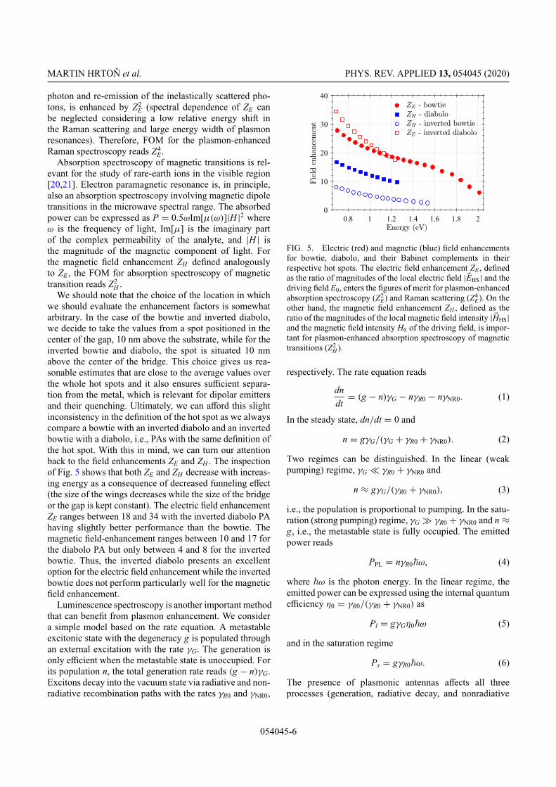
MARTIN HRTON et al. PHYS. REV. APPLIED 13, 054045 (2020)

photon and re-emission of the inelastically scattered pho-tons, is enhanced by Z2

E (spectral dependence of ZE canbe neglected considering a low relative energy shift inthe Raman scattering and large energy width of plasmonresonances). Therefore, FOM for the plasmon-enhancedRaman spectroscopy reads Z4

E .Absorption spectroscopy of magnetic transitions is rel-

evant for the study of rare-earth ions in the visible region[20,21]. Electron paramagnetic resonance is, in principle,also an absorption spectroscopy involving magnetic dipoletransitions in the microwave spectral range. The absorbedpower can be expressed as P = 0.5ωIm[μ(ω)]|H |2 whereω is the frequency of light, Im[μ] is the imaginary partof the complex permeability of the analyte, and |H | isthe magnitude of the magnetic component of light. Forthe magnetic field enhancement ZH defined analogouslyto ZE , the FOM for absorption spectroscopy of magnetictransition reads Z2

H .We should note that the choice of the location in which

we should evaluate the enhancement factors is somewhatarbitrary. In the case of the bowtie and inverted diabolo,we decide to take the values from a spot positioned in thecenter of the gap, 10 nm above the substrate, while for theinverted bowtie and diabolo, the spot is situated 10 nmabove the center of the bridge. This choice gives us rea-sonable estimates that are close to the average values overthe whole hot spots and it also ensures sufficient separa-tion from the metal, which is relevant for dipolar emittersand their quenching. Ultimately, we can afford this slightinconsistency in the definition of the hot spot as we alwayscompare a bowtie with an inverted diabolo and an invertedbowtie with a diabolo, i.e., PAs with the same definition ofthe hot spot. With this in mind, we can turn our attentionback to the field enhancements ZE and ZH . The inspectionof Fig. 5 shows that both ZE and ZH decrease with increas-ing energy as a consequence of decreased funneling effect(the size of the wings decreases while the size of the bridgeor the gap is kept constant). The electric field enhancementZE ranges between 18 and 34 with the inverted diabolo PAhaving slightly better performance than the bowtie. Themagnetic field-enhancement ranges between 10 and 17 forthe diabolo PA but only between 4 and 8 for the invertedbowtie. Thus, the inverted diabolo presents an excellentoption for the electric field enhancement while the invertedbowtie does not perform particularly well for the magneticfield enhancement.

Luminescence spectroscopy is another important methodthat can benefit from plasmon enhancement. We considera simple model based on the rate equation. A metastableexcitonic state with the degeneracy g is populated throughan external excitation with the rate γG. The generation isonly efficient when the metastable state is unoccupied. Forits population n, the total generation rate reads (g − n)γG.Excitons decay into the vacuum state via radiative and non-radiative recombination paths with the rates γR0 and γNR0,

FIG. 5. Electric (red) and magnetic (blue) field enhancementsfor bowtie, diabolo, and their Babinet complements in theirrespective hot spots. The electric field enhancement ZE , definedas the ratio of magnitudes of the local electric field |EHS| and thedriving field E0, enters the figures of merit for plasmon-enhancedabsorption spectroscopy (Z2

E) and Raman scattering (Z4E). On the

other hand, the magnetic field enhancement ZH , defined as theratio of the magnitudes of the local magnetic field intensity | HHS|and the magnetic field intensity H0 of the driving field, is impor-tant for plasmon-enhanced absorption spectroscopy of magnetictransitions (Z2

H ).

respectively. The rate equation reads

dndt

= (g − n)γG − nγR0 − nγNR0. (1)

In the steady state, dn/dt = 0 and

n = gγG/(γG + γR0 + γNR0). (2)

Two regimes can be distinguished. In the linear (weakpumping) regime, γG γR0 + γNR0 and

n ≈ gγG/(γR0 + γNR0), (3)

i.e., the population is proportional to pumping. In the satu-ration (strong pumping) regime, γG γR0 + γNR0 and n ≈g, i.e., the metastable state is fully occupied. The emittedpower reads

PPL = nγR0ω, (4)

where ω is the photon energy. In the linear regime, theemitted power can be expressed using the internal quantumefficiency η0 = γR0/(γR0 + γNR0) as

Pl = gγGη0ω (5)

and in the saturation regime

Ps = gγR0ω. (6)

The presence of plasmonic antennas affects all threeprocesses (generation, radiative decay, and nonradiative

054045-6

PLASMONIC ANTENNAS WITH ELECTRIC, MAGNETIC. . . PHYS. REV. APPLIED 13, 054045 (2020)

decay). The effect on generation varies from very impor-tant in the case of photoluminescence [18] to negligiblein the case of electroluminescence. In general, generationis a sequential inelastic process and cannot be describedby a simple model. For that, we do not consider plasmonenhancement of generation in the following and focus onits influence on the radiative and nonradiative decay rates.

Spontaneous emission is affected via Purcell effect [47].The emitter transfers its energy to PA where it is partiallyradiated into far field and partially dissipated. It is cus-tomary to express the rates of both processes in multiplesof the spontaneous emission rate γR0: ZR being the radia-tive enhancement and ZNR the nonradiative enhancement[48,49]. The total radiative and nonradiative decay ratesin the presence of plasmonic particles read γR = ZRγR0and γNR = ZNRγR0 + γNR0, respectively, and the internalquantum efficiency reads η = γR/(γR + γNR).

The figure of merit for plasmon-enhanced luminescence(only its emission part) is the rate of the powers emittedwith and without the presence of the PA. For the linearregime, FOM is

Fl = η/η0, (7)

while for the saturation regime it reads simply

Fs = ZR. (8)

Consequently, only emitters with a poor internal quantumefficiency can benefit from plasmon enhancement in thelinear regime while the emitters with a high internal quan-tum efficiency will suffer from the dissipation in metallic

PA. On the other hand, in the saturation regime plasmonenhancement is benefitable as long as ZR > 1.

Figure 6 shows the spectral dependence of radiative andnonradiative enhancement factors (ZR and ZNR, respec-tively) for different types of PA with the maximum fieldenhancement at 0.8 eV. A pointlike isotropic emitter (i.e.,all polarizations are involved with the same intensity) ispositioned in the center of the PA 10 nm above the sub-strate (bowtie and inverted diabolo) or 10 nm above thesurface of gold (diabolo and inverted bowtie). Such aseparation shall suppress emission quenching due to non-radiative decay of the emitter. For the electric dipole tran-sitions, a large radiative enhancement (several hundreds)is obtained for both the bowtie and inverted diabolo. Theinverted diabolo offers approximately twice larger peakenhancement [Fig. 6(a)] than the bowtie PA. However, thebowtie benefits from a much lower nonradiative enhance-ment and is thus preferable for most emitters in the linearregime [Fig. 6(c)]. For magnetic dipole transitions, the dia-bolo provides a considerably larger radiative enhancementthan the inverted bowtie, but it also suffers from the con-siderably larger nonradiative enhancement [Fig. 6(b)]. Inaddition, the resonance of the inverted bowtie is consid-erably wider, which can prioritize this type of antenna foremitters with broad spectral bands. The preferred PA typetherefore depends on specific application. We note thatthe peaks in the enhancement are spectrally shifted fromthe maximum field enhancement; the effect is particularlypronounced for the inverted bowtie.

At this point it is worthwhile to estimate the accu-racy of the electromagnetic simulations and the relevance

(a) (b)

(c) (d)

FIG. 6. Radiative and nonra-diative enhancement factors ZRand ZNR, respectively, as func-tions of the photon energy forthe (a) electric dipole transitionand (b) magnetic dipole transi-tion. The values are averagedover all possible polarizations ofthe transitions. Panels (c) and(d) then show enhancement ofthe overall quantum efficiencyfor two values of the internalquantum efficiency, namely η0 =0.9 (good emitter) and η0 = 0.05(poor emitter). Note that eventhough the radiative enhancementfor direct and inverted diabolosis significantly higher than fortheir bowtie counterparts, theirenhancement of quantum effi-ciency is due to their equallylarger nonradiative enhancementmore or less the same.

054045-7

MARTIN HRTON et al. PHYS. REV. APPLIED 13, 054045 (2020)

of their results for the experiment. Several authors com-pared experimental and calculated values of luminescenceenhancement factors in various systems, including organicdyes coupled to bowtie antennas [18] (measured, up to1340; calculated, 1690), MoS2 coupled to bowtie anten-nas [50] (measured, 980; calculated, 982), and WSe2monolayer coupled to cavity-backed slot antennas [51](measured: 340; calculated: 400). Apparently, there is areasonable agreement between simulations and experimentwith differences up to 20%. Further, the differences con-sist in a rather systematic overestimation of calculationsdue to model simplifications. Hence, the conclusions basedon the simulations shall be robust and reproducible in theexperiment.

C. Optical trapping

Apart from enhancing optical processes, electric hotspots can also serve as optical tweezers, i.e., they can beused to trap small objects. In the dipole limit, the opti-cal force that facilitates this trapping is proportional tothe gradient of the square of the electric field. Consider-ing the evanescent nature of plasmonic near fields, electrichot spots in the vicinity of plasmonic structures can lead tovery strong forces, stronger even than those encountered intightly focused beams that are routinely used to manipulateboth metallic and dielectric particles, living cells, DNA, orbacteria [52].

To estimate the strength of the trapping force providedby our structures, we calculated the energy required bya 20-nm polystyrene sphere to escape the potential wellformed by the plasmonic hot spot. Considering the smallsize of the particle, we deem it sufficient to work withinthe dipole approximation, where the potential energy of thesmall sphere reads [53]

V = −α

2

∣∣E∣

∣2

, (9)

where α is the polarizability of the polystyrene particle(permittivity 2.46). Note that we limit ourselves only tostructures with electric hot spots as the magnetic dipolemoment and consequently also the magnetic trappingpotential for such a small polystyrene particle is negligi-ble. Considering an illumination in the form of a 1-mWbeam focused into a 2-μm spot (corresponding to the inten-sity of 318 kWm−2) with the investigated structure in itscentre, the magnitudes of the trapping potential (whichwe define as the potential difference between the hot spotand when we are away from it) are plotted in Fig. 7. Asone might expect, the trapping potential mimics the fieldenhancement shown in Fig. 5, with larger values attained atlower resonance energies. Assuming that the system isat the room temperature (T = 300 K), the trapping energyat 0.8 eV becomes comparable to the thermal energy of thepolystyrene particles, which indicates that these structures

FIG. 7. Depth of the trapping potential for 20-nm polystyrenespheres induced by bowtie and inverted diabolo PAs illuminatedby the light with the intensity of 318 kWm−2. The potential isexpressed at the energy of the lowest LSPR and displayed as afunction of this energy. The dashed line indicates the thermalenergy at room temperature (kBT = 26 meV).

have a potential to serve as a dual purpose tool that is capa-ble of capturing an object and enhance its optical responseat nanoscale.

D. Materials beyond gold

To demonstrate the general validity of our results wenow discuss two other plasmonic materials: silver andzirconium nitride (ZrN). Silver is a traditional plasmonicmetal, which supports surface plasmon polaritons (SPP)in a broader spectral range than gold (up to the energy of3 eV) and exhibits slightly lower electron scattering rate.On the other hand, silver PAs are not as stable as goldPAs and can degrade over time [54]. ZrN is a semiconduc-tor from a class of transition-metal nitrides that supportsSPP in the visible spectral range (up to 3 eV) under suffi-ciently large doping [55]. The electron scattering in ZrNis significantly larger than in gold. For our simulations,the dielectric function of silver has been taken from John-son and Christy [43] and the dielectric function of thedoped ZrN has been taken from Naik et al. [55]. The elec-tron scattering time τ can be estimated from the dielectricfunction ε(ω) as τ = −Im(ε)/[ωRe(ε)], where Re and Imdenote the real and imaginary part, and ω is the angularfrequency. At the photon energy of 0.8 eV, τ reads 32 fsfor silver, 8.2 fs for gold, and 0.8 fs for ZrN.

The energies of the lowest LSPR supported by silverand ZrN PAs are shown as Figs. S1(a) and S2(a) withinthe Supplemental Material [56]. The energy is only weaklydependent on the material of the PA, with a slight blueshiftobserved for the smallest silver PAs attributed to the largeplasma frequency and the absence of interband transitionsin silver in the respective energy range. The energies ofLSPR in the Babinet-complementary PAs are nearly iden-tical, with the differences up to 10% for gold and silver.

054045-8

PLASMONIC ANTENNAS WITH ELECTRIC, MAGNETIC. . . PHYS. REV. APPLIED 13, 054045 (2020)

Notably, ZrN exhibits larger differences (up to 15%) atthe energy of 2 eV (due to proximity of the plasma fre-quency and a related zero-cross-point of the real part of thedielectric function) but very low differences (below 5%)at energies below 1 eV where ZrN rapidly approaches thelimit of perfect electric conductor.

The Q factors of the lowest LSPR supported by silverand ZrN PAs are shown as Figs. S1 and S2 within the Sup-plemental Material [56]. Typical values for silver PAs areby about 25% higher than for gold PAs, while the valuesfor ZrN PAs are about four times lower. As expected, theQ factor decreases for decreasing electron scattering time.The relation is weaker than linear, since the total plasmondamping is in addition to the collision damping contributedalso by the radiation damping and the Landau damping[57].

Figure 8 compares all three materials in terms of thefigures of merit of optical spectroscopy and trapping. Weshow the results only for the better PA of the pair sup-porting a specific hot spot, which is the inverted diaboloPA for the electric hot spot and the diabolo PA for the

magnetic hot spot. Complete characterization includingalso the bowtie and inverted bowtie PAs is provided asFigs. S1 and S2 within the Supplemental Material [56].The trends observed for gold PAs are qualitatively repro-duced for silver and ZrN PAs. Low-scattering materialsprovide better FOM. The effect is most pronounced for thedecay-rate enhancement factors, where the low scatteringresults in both high radiative decay-rate enhancement ZRand low nonradiative decay-rate enhancement ZNR.

Tables II and III summarize the FOM at the energyof 0.8 eV corresponding to the telecommunication wave-length of 1.55 μm. The dimensions of the antennas areadjusted to set the energy of the lowest LSPR to 0.8 eV(represented by the peak of the scattering cross section)so that we evaluate the resonant (maximum) values of theFOM. The antenna footprint F is defined as the area ofsmallest rectangle fully containing the antenna. Table IIpresents the FOM related to the electric hot spot: the Qfactor defined as the peak energy divided by the FWHM ofthe scattering cross section, the electric field enhancementZE , the radiative (ZR) and nonradiative (ZNR) decay-rate

(a) (b)

(c) (d)

FIG. 8. Comparison of gold, silver, and ZrN PAs. (a) Field-enhancement factors for the electric field in inverted diabolo PAs (red)and the magnetic field in diabolo PAs (blue) expressed at the energy of the lowest LSPR as functions of this energy. (b) Depth ofthe trapping potential for 20-nm polystyrene spheres induced by inverted diabolo PAs illuminated by the light with the intensity of318 kWm−2. The potential is expressed at the energy of the lowest LSPR and displayed as a function of this energy. The dashed lineindicates the thermal energy at room temperature (kBT = 26 meV). (c),(d) Radiative and nonradiative enhancement factors ZR and ZNR,respectively, as functions of the photon energy for (c) the inverted diabolo PA and the electric dipole transition and (d) the diabolo PAand the magnetic dipole transition. The values are averaged over all possible polarizations of the transitions. The energy of the lowestLSPR in the PAs is set to 0.8 eV.

054045-9

MARTIN HRTON et al. PHYS. REV. APPLIED 13, 054045 (2020)

TABLE II. Figures of merit related to the electric hot spot at the energy of 0.8 eV.

Material Geometry F [nm2] Q ZE ZR ZNR VTB [meV]

Silver i. diabolo 5.8 × 104 5.6 33 952 48 37bowtie 41 × 104 2.4 24 304 1 16

Gold i. diabolo 5.3 × 104 4.9 30 775 268 25.6bowtie 40 × 104 2.4 25 338 37 19.4

ZrN i. diabolo 5.3 × 104 2.1 12 112 350 5.7bowtie 36 × 104 1.6 16 142 140 7.3

enhancements for an electric dipole transition, and thetrapping barrier VTB defined as the depth of the trappingpotential for the illumination intensity of 318 kWm−2. Itincludes only PAs with the electric hot spot, i.e., bowtieand inverted diabolo. Table III presents the FOM relatedto the magnetic hot spot: the Q factor, the magnetic fieldenhancement ZH , and the radiative (ZR) and nonradiative(ZNR) decay-rate enhancements for a magnetic dipole tran-sition. It includes PAs with the magnetic hot spot, i.e.,inverted bowtie and diabolo.

There is a clear qualitative correlation between all FOM.Large values of Q factor correspond to a large fieldenhancement and large radiative decay enhancements,while nonradiative decay enhancements are small. Sil-ver with the highest electron scattering time of all threematerials involved in the study shows better performancecompared to gold, which is superior to ZrN, the materialwith the lowest electron scattering time. The diabolo PAsoffer better FOM (and lower footprint) than the bowtie PAsdue to reduced radiation losses. This finding holds for boththe bowtie and the inverted diabolo PAs supporting theelectric hot spot and the inverted bowtie and the diaboloPAs supporting the magnetic hot spot.

E. Babinet dimer with electromagnetic hot spot

Bowtie and diabolo PAs enhance either an electric ora magnetic component of the field, while the other com-ponent is only weakly enhanced and spatially focused. Inthis section we propose a Babinet dimer antenna that formsan electromagnetic hot spot enhancing and focusing bothcomponents of the electromagnetic field equally. The Babi-net dimer antenna is formed by a direct and an inverse PA,vertically stacked so closely that their individual electric

and magnetic hot spots overlap. We explore and com-pare two configurations, namely the Babinet bowtie dimer(BBD) [schematically depicted in Fig. 9(a)], consisting ofa bowtie on top of an inverted bowtie PA, and the Babi-net diabolo dimer (BDD) [sketched in Fig. 9(c)] madeup by an inverted diabolo on top of a diabolo PA. Inboth configurations, the upper PA is rotated with respectto the bottom one by 90 so that both of them can beexcited by the same source polarization (oriented along thelong axis of the direct PA) and the upper and bottom PAsare separated by a 10-nm spacer layer with the refractiveindex equal to 1.5. As the individual modes in the closelyspaced PAs exhibit strong interaction, the dimensions ofthe dimer constituents are adjusted so that the maximumfield enhancement occurs at 0.8 eV for both the electric andmagnetic component. For the BBD, the wing lengths of thetop (↑) and bottom (↓) PAs are set to v↑ = 110 nm andv↓ = 200 nm, while for the BDD, the optimal dimensionsread v↑ = 200 nm and v↓ = 110 nm. Note that the antennaproviding the magnetic enhancement is in both cases situ-ated underneath the one with the electric enhancement sothat the electromagnetic hot spot is directly accessible fromthe top.

Figure 9(b) demonstrates the formation of the electro-magnetic hot spot in the BBD. The dimer is illuminated bythe field polarized along the long axis of the bowtie andperpendicular to the long axis of inverted bowtie, whichresults in formation of an electric hot spot (field enhance-ment 14) around the direct bowtie and a magnetic hot spot(field enhancement 13) around the inverted bowtie. Theclosely spaced hot spots overlap, yielding the maximumsimultaneous enhancement of both fields close to 8.4 at theposition indicated by the green point in Fig. 9. The inspec-tion of Figs. 3 and 5 reveals that these values are similar

TABLE III. Figures of merit related to the magnetic hot spot at the energy of 0.8 eV.

Material Geometry F [nm2] Q ZH ZR ZNR

Silver diabolo 4.8 × 104 9.7 21 257 34i. bowtie 34 × 104 1.9 7.5 40 5

Gold diabolo 4.8 × 104 7.5 15 130 94i. bowtie 33 × 104 1.9 6.6 26 15

ZrN diabolo 4.4 × 104 2.1 5.0 11 83i. bowtie 31 × 104 1.0 3.7 8 55

054045-10

PLASMONIC ANTENNAS WITH ELECTRIC, MAGNETIC. . . PHYS. REV. APPLIED 13, 054045 (2020)

(a) (b)

(c) (d)

FIG. 9. (a) Schematic drawing of the BBD. A direct bowtie (wing length 110 nm) lies on top of an inverted bowtie (wing length200 nm), they are mutually rotated by 90 and separated by a 10-nm spacer layer. (b) Distribution of the electric (left) and magnetic(right) fields in the vicinity of the BBD. The top two subplots show the fields in a plane parallel to the individual PAs, namely insidethe spacer layer with 5-nm distance from both of them [indicated by a black dotted line in (a)]. The bottom two subplots then showthe fields in a vertical plane perpendicular to the metal bridge of the inverted bowtie. The orientation of the plane is outlined bya white dotted line in the schematic drawing in (a) and also in the top two subplots showing the fields in the horizontal plane. (c)Schematic drawing of the BDD. A direct diabolo (wing length 110 nm) lies underneath an inverted bowtie (wing length 200 nm), theyare mutually rotated by 90 and separated by a 10-nm spacer layer. The distribution of the electric (left) and the magnetic (right) fieldsaround the BDD is plotted in (d), with planar cross sections positioned and oriented in the same manner as in the case of BBD. Notethat both BBD and BDD are illuminated with a plane wave polarized along the long axes of the direct PAs and the green point marksthe position, in which the electric and magnetic field enhancements are equal in magnitude (with the value specified by the number).

to those obtained for single PAs of comparable size. Thisindicates that the enhancement mechanism based on thecharge accumulation (or the current funneling) at the wingapices is rather robust and resistant to changes in surround-ings of the PA. The other proposed design, BDD, possesseselectromagnetic hot spot as well, with maximum simul-taneous enhancement of 11, while the individual maximaread 21 (electric enhancement) and 16 (magnetic enhance-ment) [see Fig. 9(d)]. These values are again close to thoseencountered in single PAs, despite the partial screeningof the bottom diabolo by its upper counterpart. On thewhole, the better performance of isolated diabolos (at leastin terms of local field enhancement) imprints itself alsointo Babinet dimers.

So far we altogether disregard the vectorial nature ofelectromagnetic fields, which can be important in certainapplications. In the designs proposed above, the electricand magnetic fields in the hot spot are perpendicular toeach other, but one can achieve also other mutual orien-tations simply by rotating the vertically stacked antennaswith respect to each other. Such control over the local

polarization state of the light is quite valuable, especiallywhen we consider the aforementioned robustness with boththe field amplitude and orientation tightly bound to thegeometry of the PAs.

In comparison to previous proposals [58,59] and real-izations [13] of plasmonic electromagnetic hot spots, ourproposal brings two benefits. (i) It enhances both fields onequal basis, i.e., with the same amplitude, resonance fre-quency, and lateral spatial distribution. (ii) It involves twoisolated antennas, which can be adjusted independently,allowing extended tunability of the hot spot.

Interestingly, BBD can be used as Huygens meta-atoms—building blocks of metasurfaces that simultane-ously support electric and magnetic modes. Due to theso-called Kerker effect [60] the Huygens metasurfacesexhibit strongly directional scattering of light and allowachievement of metasurfaces with improved transmissionefficiency [61]. The realization of Huygens meta-atomreported by Zhang et al. [61] is composed of a directrodlike plasmonic antenna and an inverted rodlike plas-monic aperture positioned above each other, i.e., it can be

054045-11

MARTIN HRTON et al. PHYS. REV. APPLIED 13, 054045 (2020)

viewed as a BBD with bowties replaced with rods. Usingbowtie antennas instead of rods shall preserve the direc-tional scattering and enhance the light-matter couplingin the hot spot, paving the way towards multifunctionalmetasurfaces capable of simultaneous enhancement thelight-matter interaction and light manipulation with hightransmission efficiency. We note that the BBD discussedabove is optimized for the field enhancement and exhibitsrather low directionality of the scattering. Simultaneousoptimization of both quantities is a subject for furtherinvestigation.

Ref. [61] also provides a possible fabrication proto-col for the BBD. Alternatively, electron-beam lithographyoverlay process can be used [62,63].

IV. CONCLUSION

We perform a comprehensive study on the plasmonicantennas featuring electric, magnetic, and electromag-netic hot spots: bowtie and inverted diabolo, diaboloand inverted bowtie, and their dimers, respectively. Wecombine two types of electric-magnetic complementarity:bowtie and diabolo duality and Babinet’s principle.

For a specific resonance frequency, diabolo antennas aresignificantly smaller than bowtie antennas, and thus harderto fabricate but easier to integrate. For the minimum winglength of 50 nm, bowties covered the energy range up to2.0 eV while diabolos only up to 1.2 eV. Diabolo antennasalso exhibit considerably narrower resonances related toa higher Q factor as a consequence of a lower scatteringcross section.

We evaluate figures of merit for different methods ofoptical spectroscopy and for optical trapping. One of themost important figures of merit is the field enhancement inthe hot spot, which is larger for the diabolo antennas thanfor the bowtie antennas (and also for the electric field thanthe magnetic field). For the luminescence, the key figureof merit is the radiative and nonradiative decay enhance-ment. Here, diabolo antennas exhibited a slightly strongerradiative decay enhancement than bowtie antennas but alsopronouncedly stronger nonradiative enhancement, makingthe direct bowtie antenna a preferred option for the electricdipole transitions and the inverted bowties an equiva-lent alternative of the diabolo for the magnetic dipoletransitions.

As for the material composition, we find better figuresof merit for the plasmonic antennas made of materials withlower electron scattering rates. Silver is slightly better thangold, while zirconium nitride is considerably worse.

Finally, we propose Babinet dimer antennas enhancingboth the electric and magnetic field on an equal basis andforming an electromagnetic hot spot, which finds appli-cations in studies of rare earth ions, optical trapping,metamaterials, or nonlinear optics.

ACKNOWLEDGMENTS

We acknowledge the support by the Czech ScienceFoundation (Grant No. 17-25799S) and Ministry of Edu-cation, Youth and Sports of the Czech Republic (ProjectCEITEC 2020, No. LQ1601). Part of the work is supportedby European Union’s Horizon 2020 (Project PETER, No.767227).

[1] L. Novotny and N. van Hulst, Antennas for light, Nat.Photonics 5, 83 (2011).

[2] S. Nie and S. R. Emory, Probing single molecules and sin-gle nanoparticles by surface-enhanced Raman scattering,Science 275, 1102 (1997).

[3] J. R. Krenn, A. Dereux, J. C. Weeber, E. Bourillot, Y.Lacroute, J. P. Goudonnet, G. Schider, W. Gotschy, A.Leitner, F. R. Aussenegg, and C. Girard, Squeezing theOptical Near-Field Zone by Plasmon Coupling of MetallicNanoparticles, Phys. Rev. Lett. 82, 2590 (1999).

[4] J.-C. Weeber, J. R. Krenn, A. Dereux, B. Lamprecht, Y.Lacroute, and J. P. Goudonnet, Near-field observation ofsurface plasmon polariton propagation on thin metal stripes,Phys. Rev. B 64, 045411 (2001).

[5] H. Gao, Q. Cao, M. Zhu, D. Teng, and S. Shen, Nanofo-cusing of terahertz wave in a tapered hyperbolic metalwaveguide, Opt. Express 22, 32071 (2014).

[6] M. Urbieta, M. Barbry, Y. Zhang, P. Koval, D. Sánchez-Portal, N. Zabala, and J. Aizpurua, Atomic-scale lightningrod effect in plasmonic picocavities: A classical view to aquantum effect, ACS Nano 12, 585 (2018).

[7] F. Benz, M. K. Schmidt, A. Dreismann, R. Chikkaraddy,Y. Zhang, A. Demetriadou, C. Carnegie, H. Ohadi, B. deNijs, R. Esteban, J. Aizpurua, and J. J. Baumberg, Single-molecule optomechanics in “picocavities”, Science 354,726 (2016).

[8] L. Zhou, Q. Gan, F. J. Bartoli, and V. Dierolf, Direct near-field optical imaging of UV bowtie nanoantennas, Opt.Express 17, 20301 (2009).

[9] A. Lee, G. F. S. Andrade, A. Ahmed, M. L. Souza,N. Coombs, E. Tumarkin, K. Liu, R. Gordon, A. G. Brolo,and E. Kumacheva, Probing dynamic generation of hot-spots in self-assembled chains of gold nanorods by surface-enhanced Raman scattering, J. Am. Chem. Soc. 133, 7563(2011).

[10] T. Grosjean, M. Mivelle, F. I. Baida, G. W. Burr, and U. C.Fischer, Diabolo nanoantenna for enhancing and confiningthe magnetic optical field, Nano Lett. 11, 1009 (2011).

[11] M. Lorente-Crespo, L. Wang, R. Ortuno, C. García-Meca,Y. Ekinci, and A. Martínez, Magnetic hot spots in closelyspaced thick gold nanorings, Nano Lett. 13, 2654 (2013).

[12] I. C. Bicket, E. P. Bellido, S. Meuret, A. Polman, and G. A.Botton, Correlative electron energy loss spectroscopy andcathodoluminescence spectroscopy on three-dimensionalplasmonic split ring resonators, Microscopy 67, i40 (2018).

[13] Y. Chen, Y. Chen, J. Chu, and X. Xu, Bridged bowtie aper-ture antenna for producing an electromagnetic hot spot,ACS Photonics 4, 567 (2017).

[14] R. M. Bakker, D. Permyakov, Y. F. Yu, D. Markovich,R. Paniagua-Domínguez, L. Gonzaga, A. Samusev,

054045-12

PLASMONIC ANTENNAS WITH ELECTRIC, MAGNETIC. . . PHYS. REV. APPLIED 13, 054045 (2020)

Y. Kivshar, B. Luk’yanchuk, and A. I. Kuznetsov, Mag-netic and electric hotspots with silicon nanodimers, NanoLett. 15, 2137 (2015).

[15] T. Itoh, Y. S. Yamamoto, Y. Kitahama, and J. Balachan-dran, One-dimensional plasmonic hotspots located betweensilver nanowire dimers evaluated by surface-enhanced res-onance Raman scattering, Phys. Rev. B 95, 115441 (2017).

[16] Y. Tian, Z. Shuai, J. Shen, L. Zhang, S. Chen, C. Song,B. Zhao, Q. Fan, and L. Wang, Plasmonic heterodimerswith binding site-dependent hot spot for surface-enhancedRaman scattering, Small 14, 1800669 (2018).

[17] T.-H. Yang, Y.-W. Harn, M.-Y. Pan, L.-D. Huang, M.-C.Chen, B.-Y. Li, P.-H. Liu, P.-Y. Chen, C.-C. Lin, P.-K.Wei, L.-J. Chen, and J.-M. Wu, Ultrahigh density plasmonichot spots with ultrahigh electromagnetic field for improvedphotocatalytic activities, Appl. Catal. B 181, 612 (2016).

[18] A. Kinkhabwala, Z. Yu, S. Fan, Y. Avlasevich, K.Müllen, and W. E. Moerner, Large single-molecule fluo-rescence enhancements produced by a bowtie nanoantenna,Nat. Photonics 3, 654 (2009).

[19] A. Blank, E. Dikarov, R. Shklyar, and Y. Twig, Induction-detection electron spin resonance with sensitivity of 1000spins: En route to scalable quantum computations, Phys.Lett. A 377, 1937 (2013).

[20] M. Kasperczyk, S. Person, D. Ananias, L. D. Carlos, andL. Novotny, Excitation of Magnetic Dipole Transitions atOptical Frequencies, Phys. Rev. Lett. 114, 163903 (2015).

[21] A. V. Malakhovskii, S. L. Gnatchenko, I. S. Kachur,V. G. Piryatinskaya, and I. A. Gudim, Transformation of theHoFe3(BO3)4 absorption spectra at reorientation magnetictransitions and local properties in the excited 5F5 states ofthe Ho3+ ion, Phys. Rev. B 96, 224430 (2017).

[22] M. L. Juan, M. Righini, and R. Quidant, Plasmon nano-optical tweezers, Nat. Photonics 5, 349 (2011).

[23] D. R. Smith, J. B. Pendry, and M. C. K. Wiltshire, Meta-materials and negative refractive index, Science 305, 788(2004).

[24] M. W. Klein, C. Enkrich, M. Wegener, and S. Linden,Second-harmonic generation from magnetic metamaterials,Science 313, 502 (2006).

[25] K. Imura, H. Okamoto, M. K. Hossain, and M. Kitajima,Visualization of localized intense optical fields in sin-gle gold-nanoparticle assemblies and ultrasensitive Ramanactive sites, Nano Lett. 6, 2173 (2006).

[26] P. Kusch, S. Mastel, N. S. Mueller, N. Morquillas Azpiazu,S. Heeg, R. Gorbachev, F. Schedin, U. Hübner, J. I. Pas-cual, S. Reich, and R. Hillenbrand, Dual-scattering near-field microscope for correlative nanoimaging of SERS andelectromagnetic hotspots, Nano Lett. 17, 2667 (2017).

[27] N. Caselli, F. La China, W. Bao, F. Riboli, A. Gerardino,L. Li, E. H. Linfield, F. Pagliano, A. Fiore, P. J. Schuck,S. Cabrini, A. Weber-Bargioni, M. Gurioli, and F. Intonti,Deep-subwavelength imaging of both electric and magneticlocalized optical fields by plasmonic campanile nanoan-tenna, Sci. Rep. 5, 9606 (2015).

[28] P. Ghenuche, S. Cherukulappurath, T. H. Taminiau, N. F.van Hulst, and R. Quidant, Spectroscopic Mode Mappingof Resonant Plasmon Nanoantennas, Phys. Rev. Lett. 101,116805 (2008).

[29] B. Lahiri, G. Holland, V. Aksyuk, and A. Centrone,Nanoscale imaging of plasmonic hot spots and dark

modes with the photothermal-induced resonance technique,Nano Lett. 13, 3218 (2013).

[30] S. Dodson, M. Haggui, R. Bachelot, J. Plain, S. Li, andQ. Xiong, Optimizing electromagnetic hotspots in plas-monic bowtie nanoantennae, J. Phys. Chem. Lett. 4, 496(2013).

[31] K. Schraml, M. Spiegl, M. Kammerlocher, G. Bracher,J. Bartl, T. Campbell, J. J. Finley, and M. Kaniber, Opticalproperties and interparticle coupling of plasmonic bowtienanoantennas on a semiconducting substrate, Phys. Rev. B90, 035435 (2014).

[32] S. Sederberg and A. Y. Elezzabi, Nanoscale plasmoniccontour bowtie antenna operating in the mid-infrared,Opt. Express 19, 15532 (2011).

[33] B. J. Roxworthy, K. D. Ko, A. Kumar, K. H. Fung, E.K. C. Chow, G. L. Liu, N. X. Fang, and K. C. Toussaint,Application of plasmonic bowtie nanoantenna arrays foroptical trapping, stacking, and sorting, Nano Lett. 12, 796(2012).

[34] H. Guo, B. Simpkins, J. D. Caldwell, and J. Guo, Reso-nance spectra of diabolo optical antenna arrays, AIP Adv.5, 107149 (2015).

[35] V. Krápek, A. Konecná, M. Horák, F. Ligmajer, M.Stöger-Pollach, M. Hrton, J. Babocký, and T. Šikola,Independent engineering of individual plasmon modes inplasmonic dimers with conductive and capacitive coupling,Nanophotonics 9, 623 (2020).

[36] S. Cakmakyapan, N. A. Cinel, A. O. Cakmak, andE. Ozbay, Validation of electromagnetic field enhancementin near-infrared through Sierpinski fractal nanoantennas,Opt. Express 22, 19504 (2014).

[37] F. Falcone, T. Lopetegi, M. A. G. Laso, J. D. Baena,J. Bonache, M. Beruete, R. Marqués, F. Martín, andM. Sorolla, Babinet Principle Applied to the Design ofMetasurfaces and Metamaterials, Phys. Rev. Lett. 93,197401 (2004).

[38] M. Hentschel, T. Weiss, S. Bagheri, and H. Giessen, Babi-net to the half: Coupling of solid and inverse plasmonicstructures, Nano Lett. 13, 4428 (2013).

[39] A. Bitzer, A. Ortner, H. Merbold, T. Feurer, and M. Walther,Terahertz near-field microscopy of complementary planarmetamaterials: Babinet’s principle, Opt. Express 19, 2537(2011).

[40] T. Zentgraf, T. P. Meyrath, A. Seidel, S. Kaiser, H. Giessen,C. Rockstuhl, and F. Lederer, Babinet’s principle for opticalfrequency metamaterials and nanoantennas, Phys. Rev. B76, 033407 (2007).

[41] H. Mizobata, K. Ueno, H. Misawa, H. Okamoto, and K.Imura, Near-field spectroscopic properties of complemen-tary gold nanostructures: Applicability of Babinet’s princi-ple in the optical region, Opt. Express 25, 5279 (2017).

[42] M. Horák, V. Krápek, M. Hrton, A. Konecná, F. Ligma-jer, M. Stöger-Pollach, T. Šamoril, A. Paták, Z. Édes, O.Metelka, J. Babocký, and T. Šikola, Limits of Babinet’sprinciple for solid and hollow plasmonic antennas, Sci.Rep. 9, 4004 (2019).

[43] P. B. Johnson and R. W. Christy, Optical constants of thenoble metals, Phys. Rev. B 6, 4370 (1972).

[44] J. A. Scholl, A. García-Etxarri, A. L. Koh, and J. A. Dionne,Observation of quantum tunneling between two plasmonicnanoparticles, Nano Lett. 13, 564 (2013).

054045-13

MARTIN HRTON et al. PHYS. REV. APPLIED 13, 054045 (2020)

[45] M. Mivelle, I. Ibrahim, F. Baida, G. Burr, D. Nedeljkovic,D. Charraut, J.-Y. Rauch, R. Salut, and T. Grosjean, Bowtienano-aperture as interface between near-fields and a single-mode fiber, Opt. Express 18, 15964 (2010).

[46] J. Zhou, T. Koschny, M. Kafesaki, E. N. Economou, J. B.Pendry, and C. M. Soukoulis, Saturation of the MagneticResponse of Split-Ring Resonators at Optical Frequencies,Phys. Rev. Lett. 95, 223902 (2005).

[47] E. M. Purcell, Spontaneous emission probabilities at radiofrequencies, Phys. Rev. 69, 681 (1946).

[48] H. A. Atwater and A. Polman, Plasmonics for improvedphotovoltaic devices, Nat. Mater. 9, 205 (2010).

[49] Z. Édes, V. Krápek, and T. Šikola, Modeling of plasmon-enhanced photoluminescence of Si nanocrystals embeddedin thin silicon-rich oxinitride layer, Acta Phys. Pol. A 129,A70 (2016).

[50] E. Palacios, S. Park, S. Butun, L. Lauhon, and K. Aydin,Enhanced radiative emission from monolayer MoS2 filmsusing a single plasmonic dimer nanoantenna, Appl. Phys.Lett. 111, 031101 (2017).

[51] M. Eggleston, S. Desai, K. Messer, S. Madhvapathy, J.Xiao, X. Zhang, E. Yablonovitch, A. Javey, and M. C. Wu,in CLEO: 2015 (Optical Society of America, Washington,2015), p. FTu1E.5.

[52] D. Gao, W. Ding, M. Nieto-Vesperinas, X. Ding, M. Rah-man, T. Zhang, C. Lim, and C.-W. Qiu, Optical manipu-lation from the microscale to the nanoscale: Fundamentals,advances and prospects, Light: Sci. Appl. 6, e17039 (2017).

[53] L. Novotny, R. X. Bian, and X. S. Xie, Theory of Nanomet-ric Optical Tweezers, Phys. Rev. Lett. 79, 645 (1997).

[54] A. S. Baburin, A. M. Merzlikin, A. V. Baryshev, I. A.Ryzhikov, Y. V. Panfilov, and I. A. Rodionov, Silver-basedplasmonics: Golden material platform and application chal-lenges [invited], Opt. Mater. Express 9, 611 (2019).

[55] G. V. Naik, J. Kim, and A. Boltasseva, Oxides and nitridesas alternative plasmonic materials in the optical range[invited], Opt. Mater. Express 1, 1090 (2011).

[56] See Supplemental Material at http://link.aps.org/supplemental/10.1103/PhysRevApplied.13.054045 for silver andZrN plasmonic antennas.

[57] S. V. Boriskina, T. A. Cooper, L. Zeng, G. Ni, J. K. Tong,Y. Tsurimaki, Y. Huang, L. Meroueh, G. Mahan, and G.Chen, Losses in plasmonics: From mitigating energy dissi-pation to embracing loss-enabled functionalities, Adv. Opt.Photon. 9, 775 (2017).

[58] P. Yu, S. Chen, J. Li, H. Cheng, Z. Li, and J. Tian, Co-enhancing and -confining the electric and magnetic fieldsof the broken-nanoring and the composite nanoring byazimuthally polarized excitation, Opt. Express 21, 20611(2013).

[59] B. J. Roxworthy and K. C. Toussaint, Simultaneouslytuning the electric and magnetic plasmonic responseusing capped bi-metallic nanoantennas, Nanoscale 6, 2270(2014).

[60] M. Kerker, D.-S. Wang, and C. L. Giles, Electromagneticscattering by magnetic spheres, J. Opt. Soc. Am. 73, 765(1983).

[61] J. Zhang, M. ElKabbash, R. Wei, S. C. Singh, B. Lam,and C. Guo, Plasmonic metasurfaces with 42.3% trans-mission efficiency in the visible, Light Sci. Appl. 8, 53(2019).

[62] G. Yoon, I. Kim, S. So, J. Mun, M. Kim, and J. Rho, Fab-rication of three-dimensional suspende, interlayered andhierarchical nanostructures by accuracy-improved electronbeam lithography overlayd, Sci. Rep. 7, 6668 (2017).

[63] N. Liu, H. Guo, L. Fu, S. Kaiser, H. Schweizer, andH. Giessen, Three-dimensional photonic metamaterials atoptical frequencies, Nat. Mater. 7, 31 (2007).

054045-14