ELT-43306 Advanced Course in Digital Transmission – Fall 2013

Diversity Techniques

Markku Renfors Department of Electronics and Communications Engineering

Tampere University of Technology, Finland

Contents: • Forms of diversity • Diversity combining methods • Performance analysis of basic diversity schemes • Outage probability, Outage capacity • Further discussion about diversity concepts

o Connections with ARQ schemes o Resource usage

Main references: [1] Simon Haykin, Digital Communication Systems. Wiley 2013. [2] Andrea Goldsmith, Wireless Communications. Cambridge University Press, 2005. [3] J.G. Proakis, Digital Communications,4th ed., McGraw-Hill, 2001. [4] Earlier lecture notes of the course by Jukka Rinne.

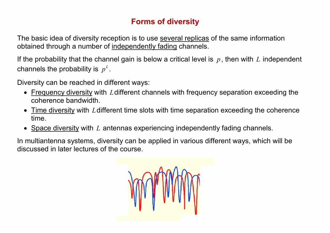
Forms of diversity The basic idea of diversity reception is to use several replicas of the same information obtained through a number of independently fading channels.

If the probability that the channel gain is below a critical level is p , then with L independent channels the probability is Lp .

Diversity can be reached in different ways: • Frequency diversity with Ldifferent channels with frequency separation exceeding the

coherence bandwidth. • Time diversity with Ldifferent time slots with time separation exceeding the coherence

time. • Space diversity with L antennas experiencing independently fading channels.

In multiantenna systems, diversity can be applied in various different ways, which will be discussed in later lectures of the course.

System model

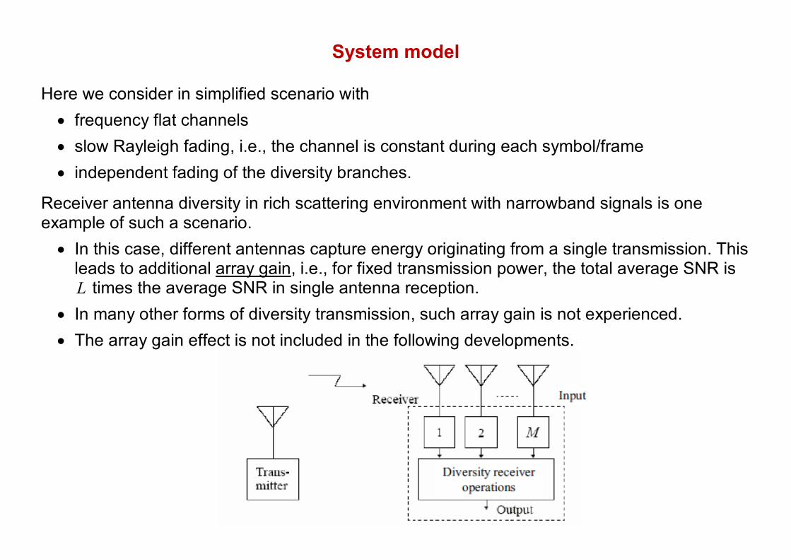
Here we consider in simplified scenario with • frequency flat channels • slow Rayleigh fading, i.e., the channel is constant during each symbol/frame • independent fading of the diversity branches.

Receiver antenna diversity in rich scattering environment with narrowband signals is one example of such a scenario.

• In this case, different antennas capture energy originating from a single transmission. This leads to additional array gain, i.e., for fixed transmission power, the total average SNR is L times the average SNR in single antenna reception.

• In many other forms of diversity transmission, such array gain is not experienced. • The array gain effect is not included in the following developments.

Notations

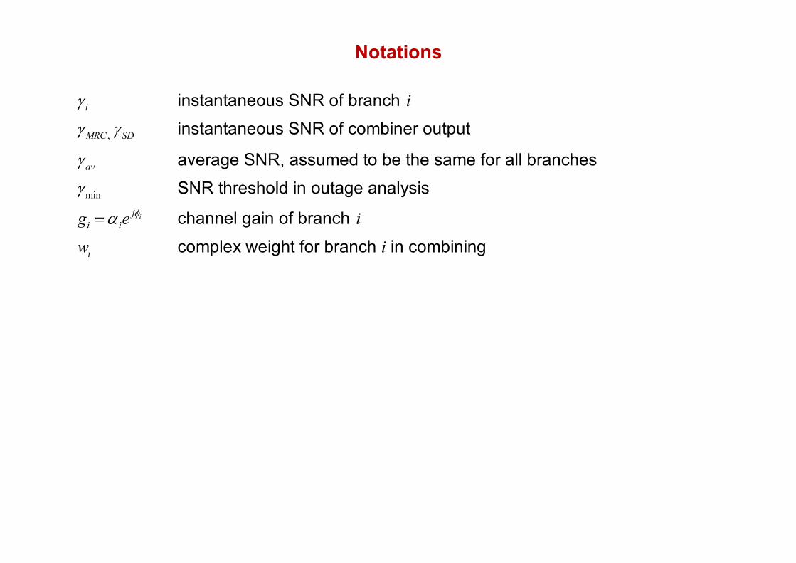
iγ instantaneous SNR of branch i

,MRC SDγ γ instantaneous SNR of combiner output

avγ average SNR, assumed to be the same for all branches

minγ SNR threshold in outage analysis ij

i ig e φα= channel gain of branch i

iw complex weight for branch i in combining

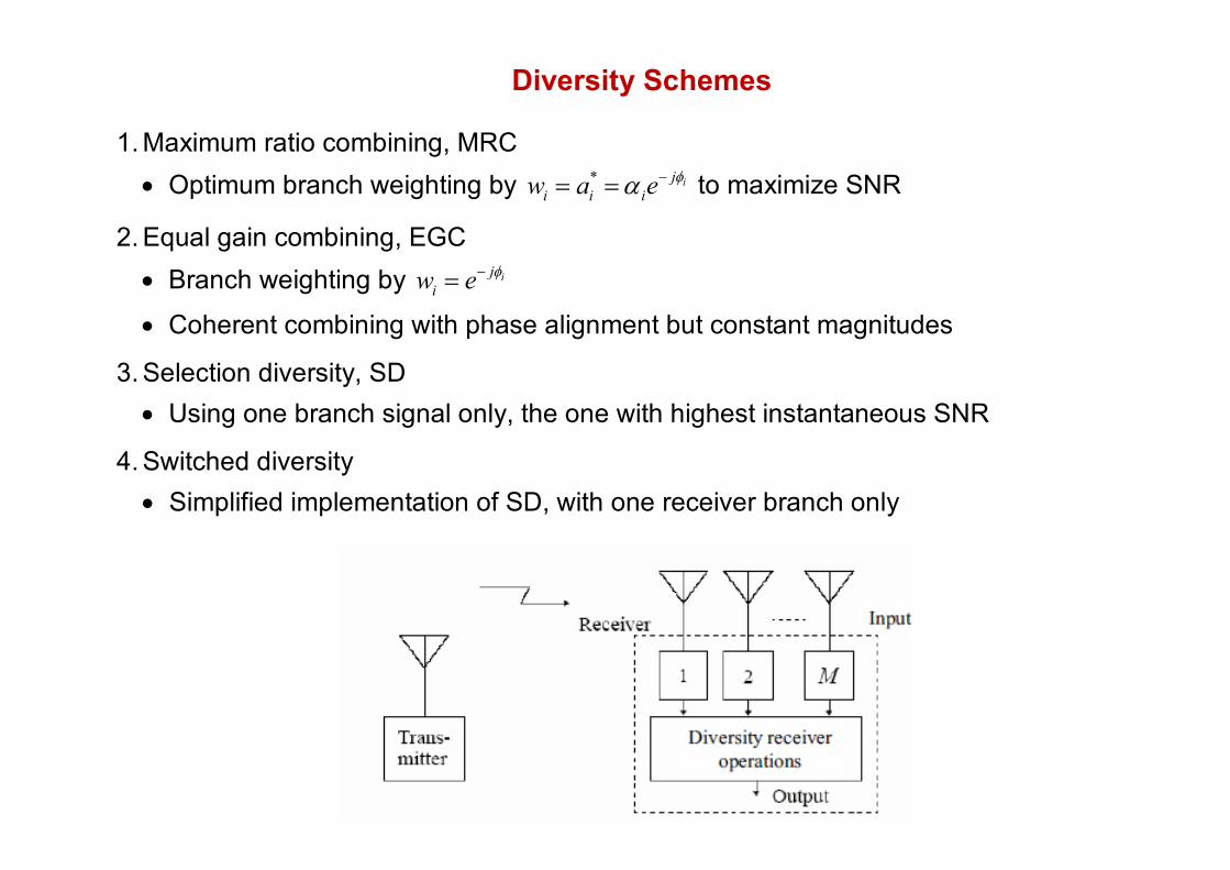
Diversity Schemes 1. Maximum ratio combining, MRC

• Optimum branch weighting by * iji i iw a e φα −= = to maximize SNR

2. Equal gain combining, EGC • Branch weighting by ij

iw e φ−=

• Coherent combining with phase alignment but constant magnitudes

3. Selection diversity, SD • Using one branch signal only, the one with highest instantaneous SNR

4. Switched diversity • Simplified implementation of SD, with one receiver branch only

Exercise: Brute-force analysis of MRC

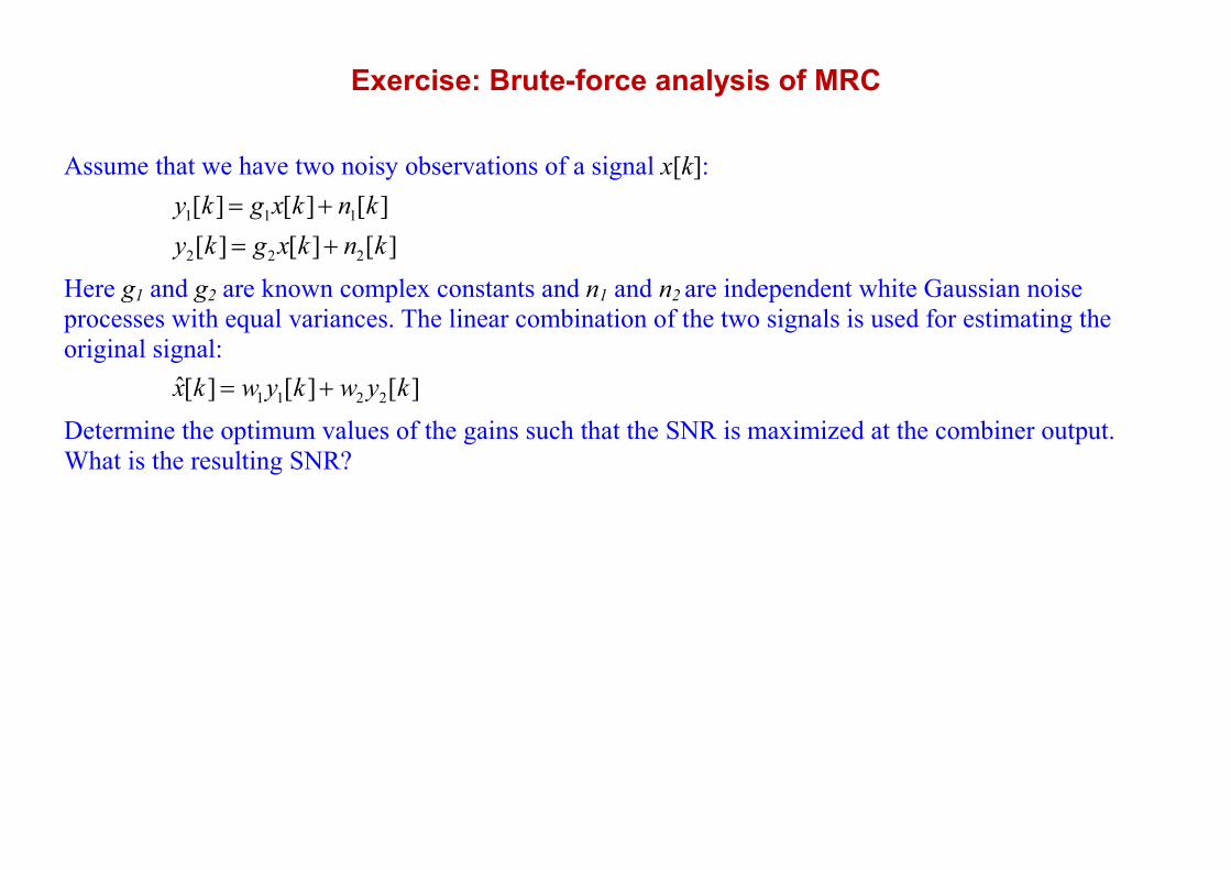
Assume that we have two noisy observations of a signal x[k]:

1 1 1

2 2 2

[ ] [ ] [ ][ ] [ ] [ ]

y k g x k n ky k g x k n k

= += +

Here g1 and g2 are known complex constants and n1 and n2 are independent white Gaussian noise processes with equal variances. The linear combination of the two signals is used for estimating the original signal: 1 1 2 2ˆ[ ] [ ] [ ]x k w y k w y k= + Determine the optimum values of the gains such that the SNR is maximized at the combiner output. What is the resulting SNR?

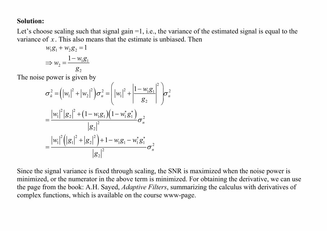
Solution: Let’s choose scaling such that signal gain =1, i.e., the variance of the estimated signal is equal to the variance of x . This also means that the estimate is unbiased. Then

1 1 2 2

1 12

2

11

w g w gw gwg

+ =−

⇒ =

The noise power is given by

( )( )( )

( )

22 2 22 2 21 1

ˆ 1 2 12

2 21 2 1 1 1 1 2

22

2 2 21 1 2 1 1 1 1 2

22

1

1 1

1

n n n

n

n

w gw w wg

w g w g w g

g

w g g w g w g

g

σ σ σ

σ

σ

∗ ∗

∗ ∗

− = + = +

+ − −=

+ + − −=

Since the signal variance is fixed through scaling, the SNR is maximized when the noise power is minimized, or the numerator in the above term is minimized. For obtaining the derivative, we can use the page from the book: A.H. Sayed, Adaptive Filters, summarizing the calculus with derivatives of complex functions, which is available on the course www-page.

( )( ) ( )

( )

( )

2 2 21 1 2 1 1 1 1 2 2 *

1 2 1 11

*1

1 2 21 2

*2

2 2 21 2

10

w g g w g w gg g w g

wgw

g g

gwg g

∗ ∗∂ + + − −= + − =

∂

⇒ =+

⇒ =+

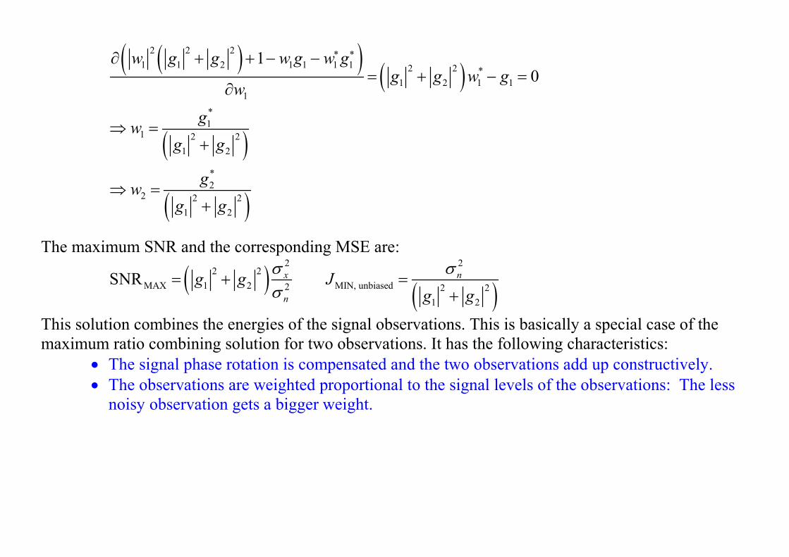
The maximum SNR and the corresponding MSE are:

( ) ( )2 2

2 2MAX 1 2 MIN, unbiased2 2 2

1 2

SNR x n

n

g g Jg g

σ σσ

= + =+

This solution combines the energies of the signal observations. This is basically a special case of the maximum ratio combining solution for two observations. It has the following characteristics:

• The signal phase rotation is compensated and the two observations add up constructively. • The observations are weighted proportional to the signal levels of the observations: The less

noisy observation gets a bigger weight.

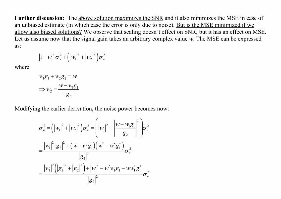
Further discussion: The above solution maximizes the SNR and it also minimizes the MSE in case of an unbiased estimate (in which case the error is only due to noise). But is the MSE minimized if we allow also biased solutions? We observe that scaling doesn’t effect on SNR, but it has an effect on MSE. Let us assume now that the signal gain takes an arbitrary complex value w. The MSE can be expressed as:

( )2 2 22 21 21 x nw w wσ σ− + +

where

1 1 2 2

1 12

2

w g w g ww w gw

g

+ =−

⇒ =

Modifying the earlier derivation, the noise power becomes now:

( )( )( )

( )

22 2 22 2 21 1

ˆ 1 2 12

2 2 *1 2 1 1 1 1 2

22

2 2 2 2 *1 1 2 1 1 1 1 2

22

n n n

n

n

w w gw w wg

w g w w g w w g

g

w g g w w w g ww g

g

σ σ σ

σ

σ

∗ ∗

∗ ∗

− = + = +

+ − −=

+ + − −=

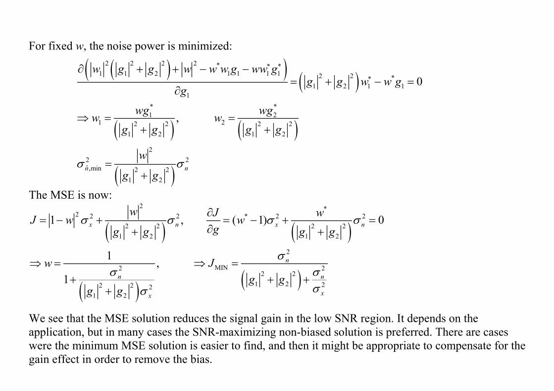
For fixed w, the noise power is minimized:

( )( ) ( )

( ) ( )

( )

2 2 2 2 *1 1 2 1 1 1 1 2 2 *

1 2 1 11

* *1 2

1 22 2 2 21 2 1 2

22 2ˆ,min 2 2

1 2

0

,

n n

w g g w w w g ww gg g w w g

gwg wgw w

g g g g

w

g gσ σ

∗ ∗

∗∂ + + − −

= + − =∂

⇒ = =+ +

=+

The MSE is now:

( ) ( )

( ) ( )

2 *2 2 2 * 2 2

2 2 2 21 2 1 2

2

MIN2 22 2

1 2 22 2 21 2

1 , ( 1) 0

1 ,1

x n x n

n

n n

xx

w J wJ w wgg g g g

w Jg g

g g

σ σ σ σ

σσ σ

σσ

∂= − + = − + =

∂+ +

⇒ = ⇒ =+ + +

+

We see that the MSE solution reduces the signal gain in the low SNR region. It depends on the application, but in many cases the SNR-maximizing non-biased solution is preferred. There are cases were the minimum MSE solution is easier to find, and then it might be appropriate to compensate for the gain effect in order to remove the bias.

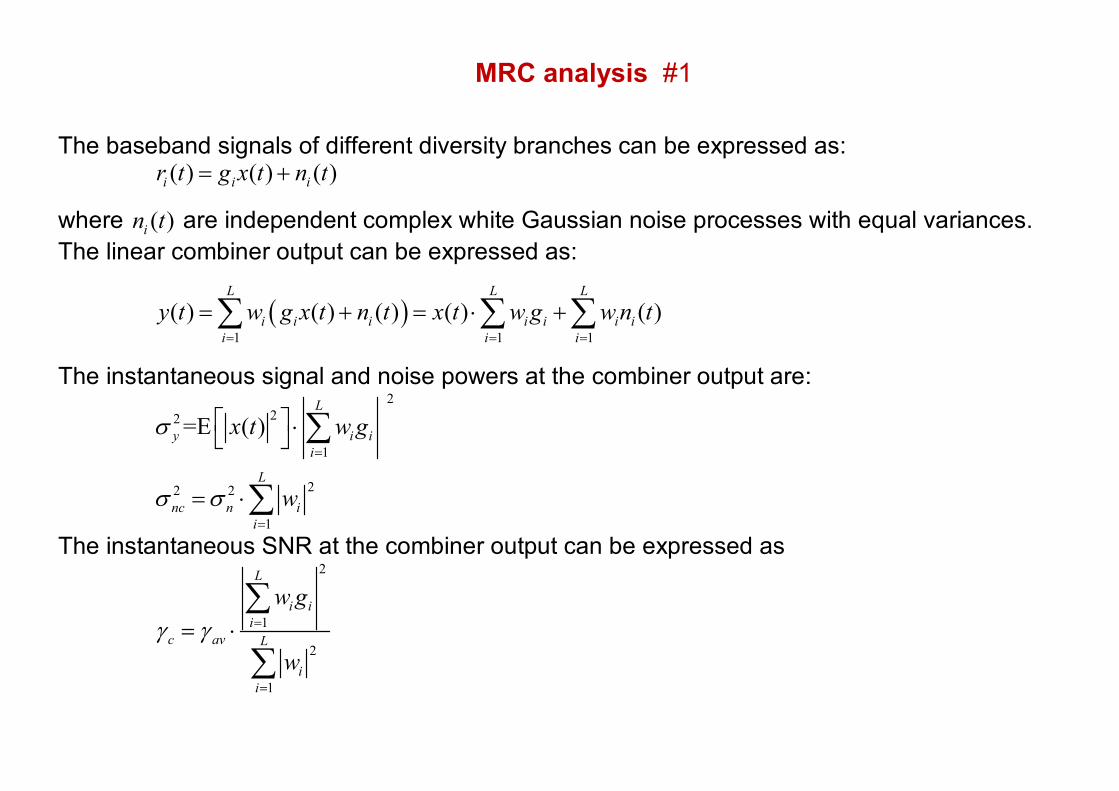
MRC analysis #1

The baseband signals of different diversity branches can be expressed as: ( ) ( ) ( )i i ir t g x t n t= +

where ( )in t are independent complex white Gaussian noise processes with equal variances. The linear combiner output can be expressed as:

( )1 1 1

( ) ( ) ( ) ( ) ( )L L L

i i i i i i ii i i

y t w g x t n t x t w g w n t= = =

= + = ⋅ +∑ ∑ ∑

The instantaneous signal and noise powers at the combiner output are: 2

22

1

22 2

1

=E ( )L

y i ii

L

nc n ii

x t w g

w

σ

σ σ

=

=

⋅

= ⋅

∑

∑

The instantaneous SNR at the combiner output can be expressed as 2

1

2

1

L

i ii

c av L

ii

w g

wγ γ =

=

= ⋅∑

∑

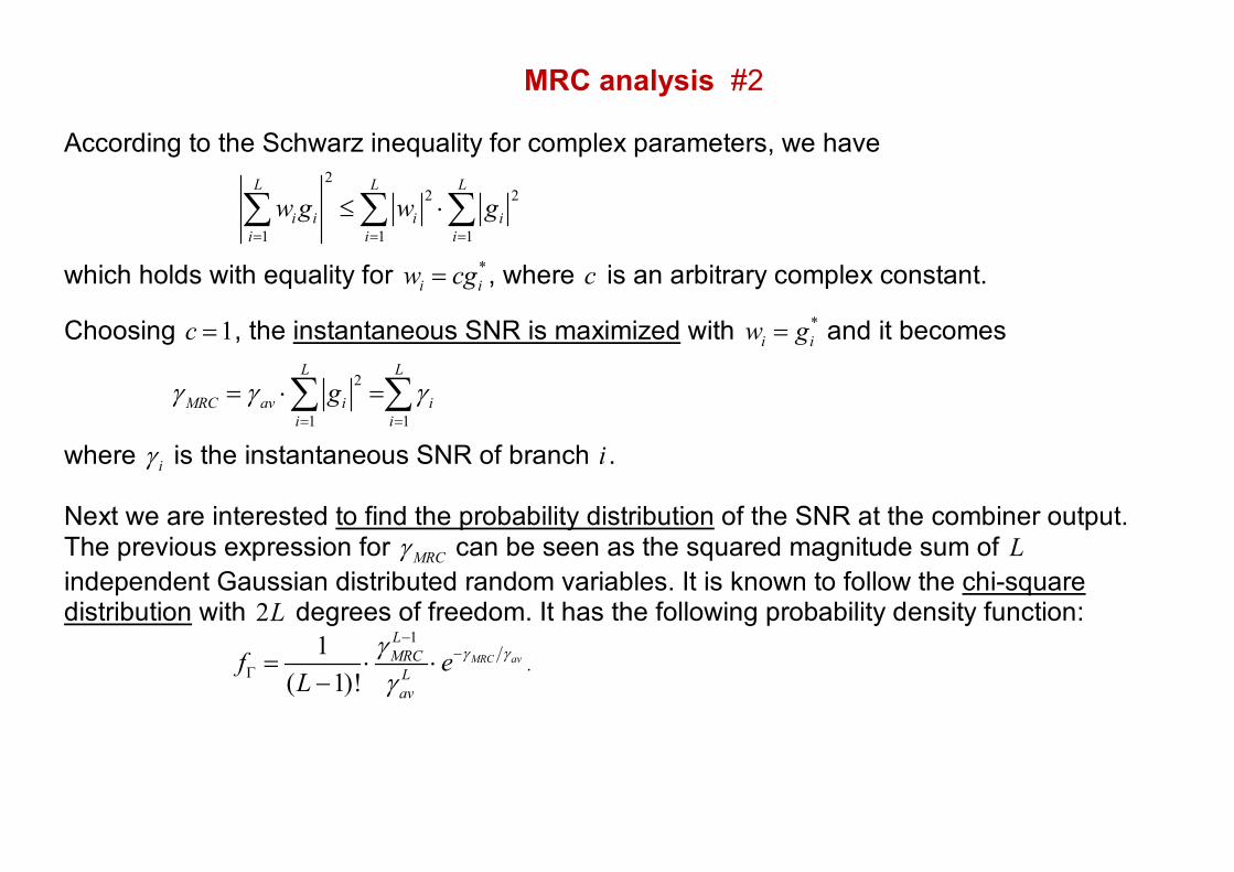
MRC analysis #2

According to the Schwarz inequality for complex parameters, we have

22 2

1 1 1

L L L

i i i ii i i

w g w g= = =

≤ ⋅∑ ∑ ∑

which holds with equality for *i iw cg= , where c is an arbitrary complex constant.

Choosing 1c = , the instantaneous SNR is maximized with *i iw g= and it becomes

2

1 1

L L

MRC av i ii i

gγ γ γ= =

= ⋅ =∑ ∑

where iγ is the instantaneous SNR of branch i .

Next we are interested to find the probability distribution of the SNR at the combiner output. The previous expression for MRCγ can be seen as the squared magnitude sum of L independent Gaussian distributed random variables. It is known to follow the chi-square distribution with 2L degrees of freedom. It has the following probability density function:

11

( 1)!MRC av

LMRC

Lav

f eL

γ γγγ

−−

Γ = ⋅ ⋅−

.

MRC analysis #3

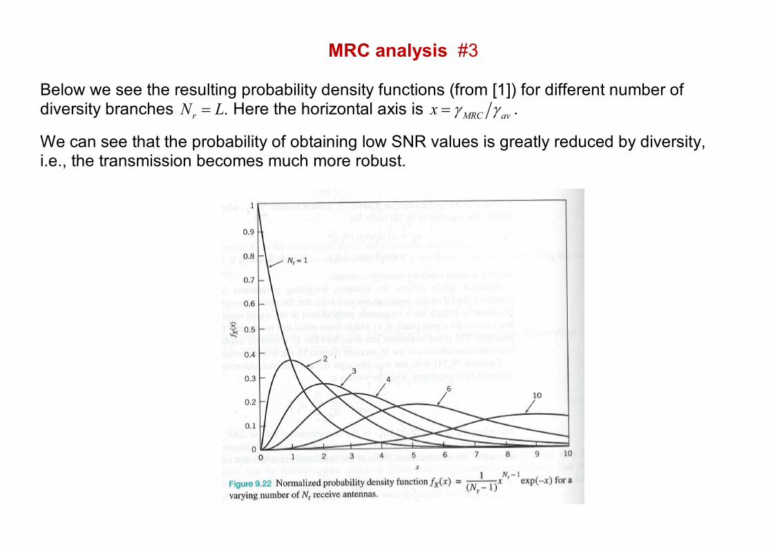
Below we see the resulting probability density functions (from [1]) for different number of diversity branches .rN L= Here the horizontal axis is MRC avx γ γ= .

We can see that the probability of obtaining low SNR values is greatly reduced by diversity, i.e., the transmission becomes much more robust.

MRC analysis #4

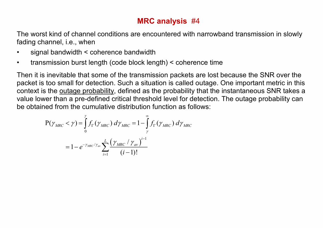
The worst kind of channel conditions are encountered with narrowband transmission in slowly fading channel, i.e., when • signal bandwidth < coherence bandwidth • transmission burst length (code block length) < coherence time

Then it is inevitable that some of the transmission packets are lost because the SNR over the packet is too small for detection. Such a situation is called outage. One important metric in this context is the outage probability, defined as the probability that the instantaneous SNR takes a value lower than a pre-defined critical threshold level for detection. The outage probability can be obtained from the cumulative distribution function as follows:

( )0

1/

1

P( ) ( ) 1 ( )

/1

( 1)!MRC av

MRC MRC MRC MRC MRC

iLMRC av

i

f d f d

ei

γ

γ

γ γ

γ γ γ γ γ γ

γ γ

∞

Γ Γ

−−

=

< = = −

= −−

∫ ∫

∑

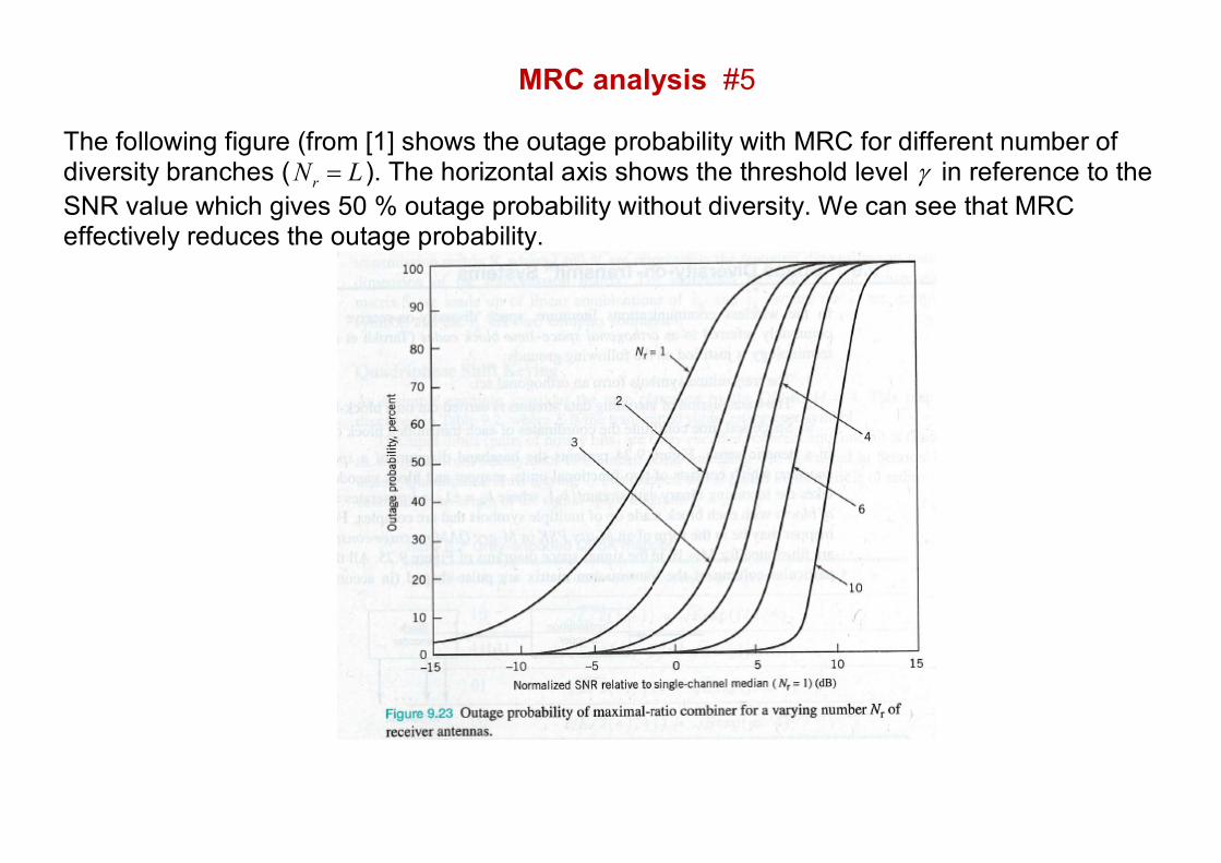
MRC analysis #5 The following figure (from [1] shows the outage probability with MRC for different number of diversity branches ( rN L= ). The horizontal axis shows the threshold level γ in reference to the SNR value which gives 50 % outage probability without diversity. We can see that MRC effectively reduces the outage probability.

Selection diversity analysis #1

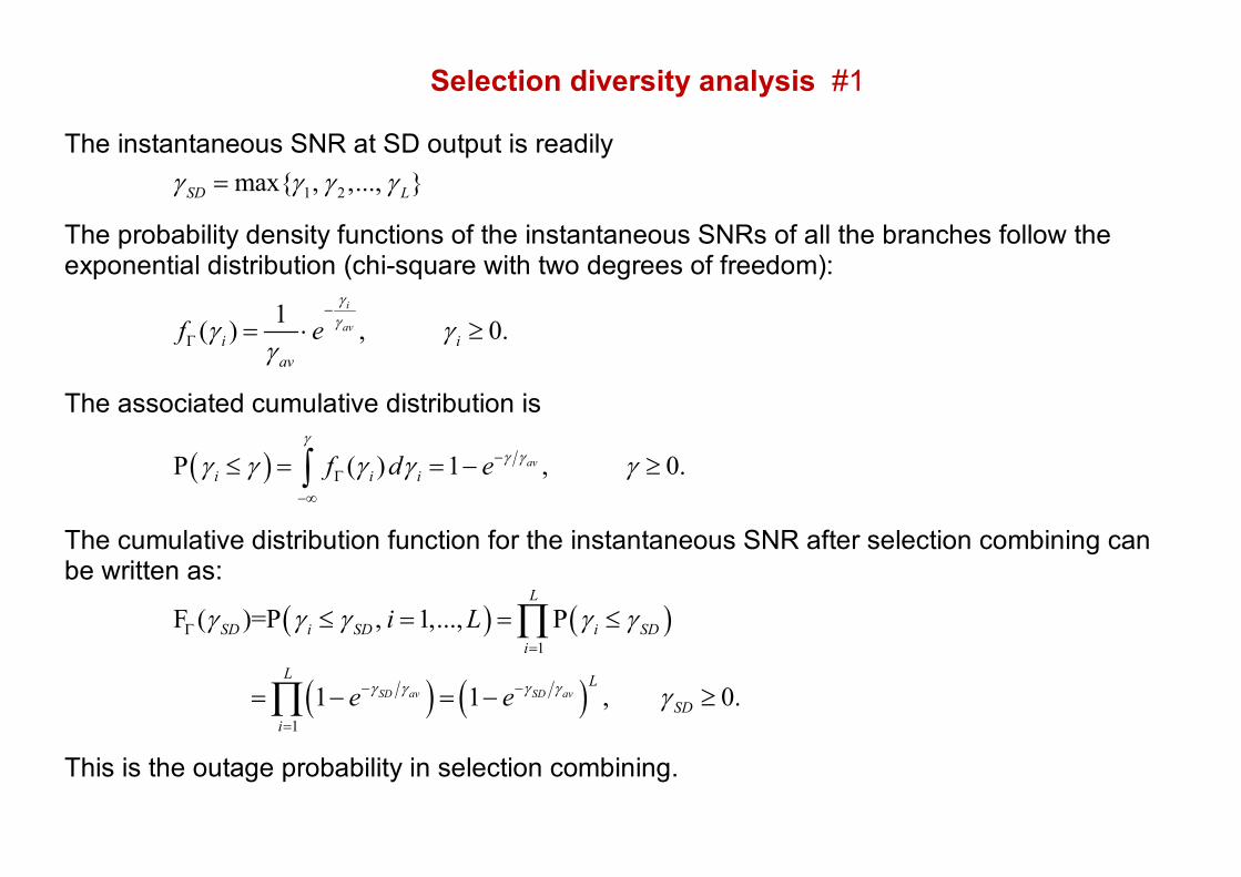
The instantaneous SNR at SD output is readily

1 2max{ , ,..., }SD Lγ γ γ γ=

The probability density functions of the instantaneous SNRs of all the branches follow the exponential distribution (chi-square with two degrees of freedom):

1( ) , 0.i

avi i

av

f eγγγ γ

γ

−

Γ = ⋅ ≥

The associated cumulative distribution is

( )P ( ) 1 , 0.avi i if d e

γγ γγ γ γ γ γ−

Γ−∞

≤ = = − ≥∫

The cumulative distribution function for the instantaneous SNR after selection combining can be written as:

( ) ( )

( ) ( )1

1

F ( )=P , 1,..., P

1 1 , 0.SD av SD av

L

SD i SD i SDi

L L

SDi

i L

e eγ γ γ γ

γ γ γ γ γ

γ

Γ=

− −

=

≤ = = ≤

= − = − ≥

∏

∏

This is the outage probability in selection combining.

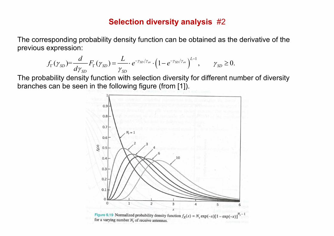
Selection diversity analysis #2 The corresponding probability density function can be obtained as the derivative of the previous expression:

( ) 1( )= ( ) 1 , 0.SD av SD av

L

SD SD SDSD SD

d Lf F e ed

γ γ γ γγ γ γγ γ

−− −Γ Γ = ⋅ ⋅ − ≥

The probability density function with selection diversity for different number of diversity branches can be seen in the following figure (from [1]).

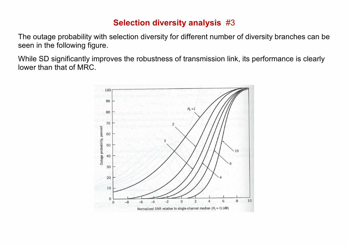
Selection diversity analysis #3 The outage probability with selection diversity for different number of diversity branches can be seen in the following figure.

While SD significantly improves the robustness of transmission link, its performance is clearly lower than that of MRC.

Numerical example of diversity gains

As an example, for 10 % outage probability, diversity order 4 with MRC gives about 12 dB reduction in the needed average SNR compared to the SNR needed in the no diversity case. With selection combining, the gain is about 9 dB. In receiver antenna diversity, these are also the gains in the total transmission power, assuming that the diversity paths are independently fading.

In other diversity schemes, the transmission power has to be split between the diversity branches, and the corresponding gains become about 6 dB for MRC and 3 dB for SC.

BER analysis

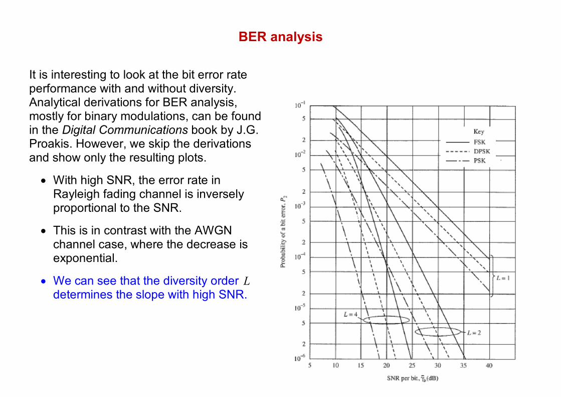
It is interesting to look at the bit error rate performance with and without diversity. Analytical derivations for BER analysis, mostly for binary modulations, can be found in the Digital Communications book by J.G. Proakis. However, we skip the derivations and show only the resulting plots.

• With high SNR, the error rate in Rayleigh fading channel is inversely proportional to the SNR.

• This is in contrast with the AWGN channel case, where the decrease is exponential.

• We can see that the diversity order L determines the slope with high SNR.

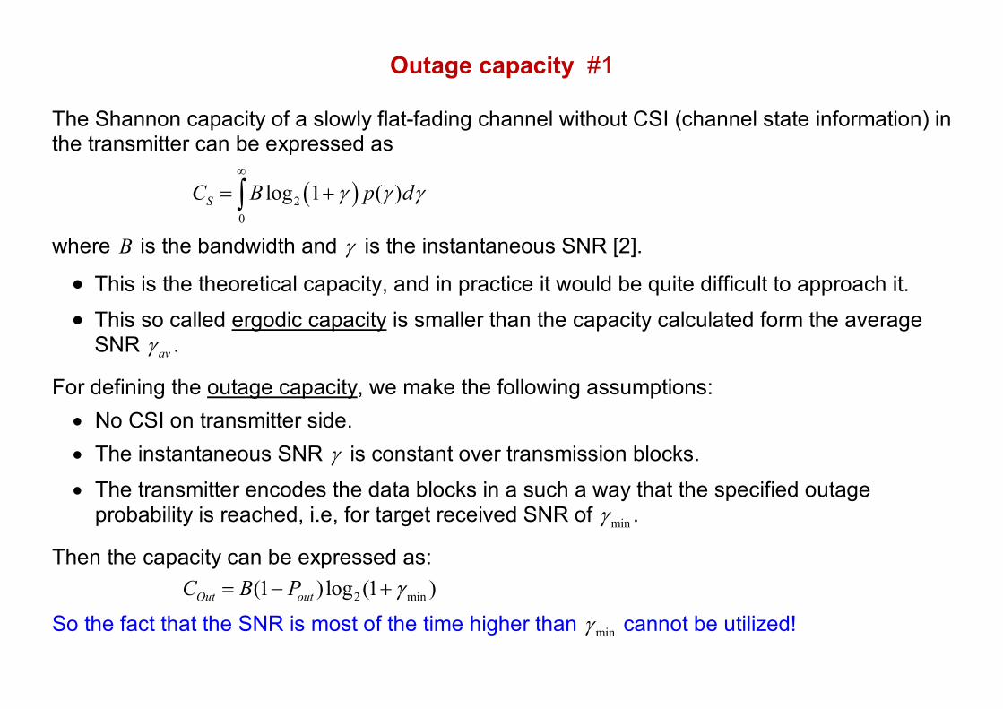
Outage capacity #1

The Shannon capacity of a slowly flat-fading channel without CSI (channel state information) in the transmitter can be expressed as

( )20

log 1 ( )SC B p dγ γ γ∞

= +∫

where B is the bandwidth and γ is the instantaneous SNR [2].

• This is the theoretical capacity, and in practice it would be quite difficult to approach it. • This so called ergodic capacity is smaller than the capacity calculated form the average

SNR avγ .

For defining the outage capacity, we make the following assumptions: • No CSI on transmitter side. • The instantaneous SNR γ is constant over transmission blocks.

• The transmitter encodes the data blocks in a such a way that the specified outage probability is reached, i.e, for target received SNR of minγ .

Then the capacity can be expressed as: 2 min(1 ) log (1 )Out outC B P γ= − +

So the fact that the SNR is most of the time higher than minγ cannot be utilized!

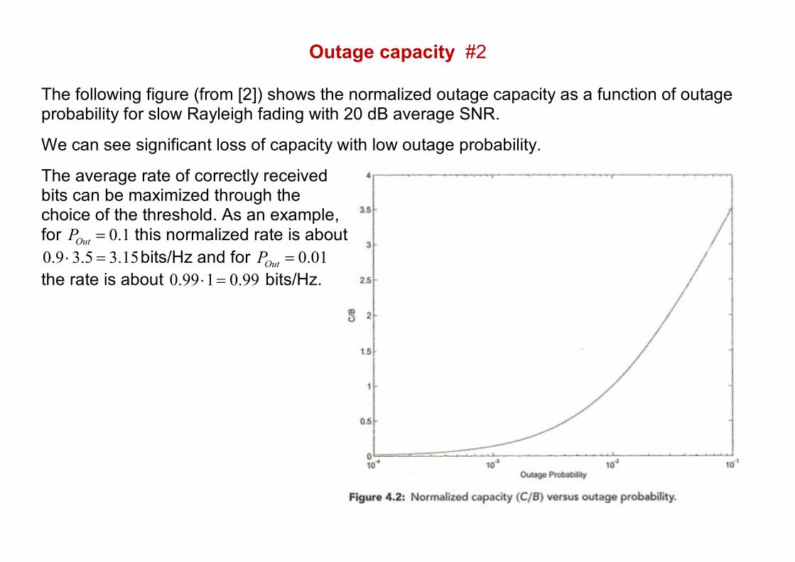
Outage capacity #2

The following figure (from [2]) shows the normalized outage capacity as a function of outage probability for slow Rayleigh fading with 20 dB average SNR.

We can see significant loss of capacity with low outage probability.

The average rate of correctly received bits can be maximized through the choice of the threshold. As an example, for 0.1OutP = this normalized rate is about 0.9 3.5 3.15⋅ = bits/Hz and for 0.01OutP = the rate is about 0.99 1 0.99⋅ = bits/Hz.

About diversity concepts #1

Narrowband transmission in slowly fading channel is essentially the most difficult case, especially regarding the outage probability. There is basically no diversity!

There are various approaches to include diversity in the transmission: • frequency diversity using coded multicarrier modulation • CDMA techniques with RAKE receiver • multicarrier CDMA is basically a simple frequency diversity scheme from a single users

point of view, but it allows multiple users to share the same transmission band by using orthogonal codes.

• multiantenna techniques with spatial diversity o receiver antenna diversity o transmit diversity o MIMO

• wideband single-carrier transmission has inherent frequency diversity o the notches in frequency response don’t have catastrophic effects on performance o the RAKE receiver is another interpretation, which shows the presence of diversity in

an intuitive way o channel equalization becomes a challenge, but frequency-domain channel

equalization is considered to be a solution with realistic complexity

About diversity concepts #2

In basic diversity schemes, the same data is transmitted in different diversity branches. This can be seen as repetition coding, i.e., as a very elementary error correction coding technique. However, repetition coding has fairly high overhead in terms of spectral efficiency.

Especially in CDMA schemes, a certain number of users are using the same frequency band at the same time, thus improving the system spectral efficiency, while exploiting frequency diversity. The interferences between users are ideally avoided by using orthogonal codes. However, the orthogonality is usually lost in practice due to various reasons, leading to the need for more complicated detection techniques for optimum system performance.

An alternative approach is to combine diversity in some form with more efficient error control coding methods (e.g., LDPC or turbo-codes), instead of repetition coding. The coding can be done in such a way that the code word bits have time/frequency/spatial diversity. Such approaches lead to spectrally efficient transmission schemes with certain amount of diversity and robustness against fading, and reduced outage probability.

Diversity and ARQ ARQ (automatic repeat request) schemes can also be considered in the context of diversity, like ‘diversity on demand’:

• If it is not possible to detect the received data frame, then a retransmission is requested. • Basic ARQ is associated with selection diversity, i.e., the earlier transmissions are ignored

and only the latest one is used for detection. • In HARQ (hybrid ARQ), information about all received data packets is combined to

improve detection performance. Among various other schemes, diversity combing methods could be considered as possible ways of combining them. However, in advanced HARQ schemes, the data carried by retransmission is usually incremental, i.e., not the same as the original data packet.

Outage capacity considerations in the ARQ context help us also to understand the dimensioning of modern wireless systems:

• Outage probability with no diversity gives us the probability of (first) retransmission. On the other hand, we have seen that low outage probability results in low capacity. Then it becomes obvious that fairly frequent retransmissions might be acceptable to maximize the capacity.

• In fact the optimization of current wireless systems (which typically include HARQ) has resulted in parametrizations where the coded block error rate is in the order of 5 … 10 %. The uncoded BER is typically in the same order, and coded BER in the order of 0.0001 … 0.001.

Diversity and resource usage In receiver antenna diversity, the diversity gain is achieved without a need for additional transmission resources, in terms of bandwidth/spectrum efficiency or transmission energy. Of course, multiple antennas and multiple receiver chains are needed in the receiver.

In transmit (antenna) diversity, the goal is to reach the diversity gain without losing spectrum efficiency. This is possible in some specific cases (notably using the Alamouti code with two antennas), but not generally. In transmit diversity, the overall transmission energy is split between diversity branches (transmit antennas). Multiple transmitters are needed, however, with reduced power level if the overall transmission power is fixed.

In basic frequency diversity or time diversity schemes, additional spectral resources are needed to reach diversity. Also here, the overall transmission energy is split between diversity branches.

Various coding schemes are aiming at good compromise between time/frequency diversity and spectrum efficiency.

In ARQ schemes, diversity is included in terms of retransmissions, when needed. The effect on spectrum efficiency and energy consumption depends on the retransmission probability.