musical techniques
TRANSCRIPT

Musical Techniques

Musical Techniques
Frequencies and Harmony
Dominique Paret Serge Sibony
First published 2017 in Great Britain and the United States by ISTE Ltd and John Wiley & Sons, Inc.
Apart from any fair dealing for the purposes of research or private study, or criticism or review, as permitted under the Copyright, Designs and Patents Act 1988, this publication may only be reproduced, stored or transmitted, in any form or by any means, with the prior permission in writing of the publishers, or in the case of reprographic reproduction in accordance with the terms and licenses issued by the CLA. Enquiries concerning reproduction outside these terms should be sent to the publishers at the undermentioned address:
ISTE Ltd John Wiley & Sons, Inc. 27-37 St George’s Road 111 River Street London SW19 4EU Hoboken, NJ 07030 UK USA
www.iste.co.uk www.wiley.com
© ISTE Ltd 2017 The rights of Dominique Paret and Serge Sibony to be identified as the authors of this work have been asserted by them in accordance with the Copyright, Designs and Patents Act 1988.
Library of Congress Control Number: 2016960997 British Library Cataloguing-in-Publication Data A CIP record for this book is available from the British Library ISBN 978-1-78630-058-4

Contents
Preface . . . . . . . . . . . . . . . . . . . . . . . . . . . . . . . . . . . . . . . . . . . xiii
Introduction . . . . . . . . . . . . . . . . . . . . . . . . . . . . . . . . . . . . . . . . xv
Part 1. Laying the Foundations . . . . . . . . . . . . . . . . . . . . . . . . . . . . 1
Introduction to Part 1 . . . . . . . . . . . . . . . . . . . . . . . . . . . . . . . . . . 3
Chapter 1. Sounds, Creation and Generation of Notes . . . . . . . . . . . . . . . . . . . . . . . . . . . . . . . . . . . 5
1.1. Physical and physiological notions of a sound . . . . . . . . . . . . . . . . . . 5 1.1.1. Auditory apparatus . . . . . . . . . . . . . . . . . . . . . . . . . . . . . . . 5 1.1.2. Physical concepts of a sound . . . . . . . . . . . . . . . . . . . . . . . . . . 7 1.1.3. Further information on acoustics and acoustic physiology . . . . . . . . . . . . . . . . . . . . . . . . . . . . . . . . 8 1.1.4. Idea of minimum audible gap/interval between two frequencies . . . . . . . . . . . . . . . . . . . . . . . . . . . . . . . 16 1.1.5. Why have we told this whole story, then? . . . . . . . . . . . . . . . . . . 22
Chapter 2. Generation of Notes . . . . . . . . . . . . . . . . . . . . . . . . . . . . 23
2.1. Concept of octave . . . . . . . . . . . . . . . . . . . . . . . . . . . . . . . . . . 23 2.1.1. Choice of inner division of an octave . . . . . . . . . . . . . . . . . . . . . 24
2.2. Modes of generation/creation/construction of notes . . . . . . . . . . . . . . . 25 2.3. Physical/natural generation of notes . . . . . . . . . . . . . . . . . . . . . . . . 26
2.3.1. Harmonics . . . . . . . . . . . . . . . . . . . . . . . . . . . . . . . . . . . . 26 2.3.2. Fractional harmonics . . . . . . . . . . . . . . . . . . . . . . . . . . . . . . 26
vi Musical Techniques
2.3.3. Initial conclusions . . . . . . . . . . . . . . . . . . . . . . . . . . . . . . . . 29 2.3.4. Order of appearance and initial naming of the notes . . . . . . . . . . . . . . . . . . . . . . . . . . . . . . . . . . 29 2.3.5. A few important additional remarks . . . . . . . . . . . . . . . . . . . . . . 32
2.4. Generation of perfect fifth notes . . . . . . . . . . . . . . . . . . . . . . . . . . 33 2.4.1. Generation with ascending fifths . . . . . . . . . . . . . . . . . . . . . . . 33 2.4.2. Generation with descending fifths . . . . . . . . . . . . . . . . . . . . . . . 37 2.4.3. Conclusions on fifth-based constructions of notes . . . . . . . . . . . . . . . . . . . . . . . . . . . . . . . . . 39
2.5. Important remarks on “physical”/”fifths” generation . . . . . . . . . . . . . . . 40 2.6. Generation of tempered notes . . . . . . . . . . . . . . . . . . . . . . . . . . . . 40
2.6.1. Notion of the ear’s logarithmic sensitivity . . . . . . . . . . . . . . . . . . 41 2.6.2. Examples of electronic generation of tempered notes . . . . . . . . . . . . . . . . . . . . . . . . . . . . . . . . . . . . . 43 2.6.3. Relative gaps between tempered and electronic notes . . . . . . . . . . . . . . . . . . . . . . . . . . . . . . . . . . 43
2.7. In summary and in conclusion on generation of notes . . . . . . . . . . . . . . . . . . . . . . . . . . . . . . . . . . . . 46 2.8. Comparison of gaps between all the notes thus created . . . . . . . . . . . . . . . . . . . . . . . . . . . . . . . . . . . . . 49
2.8.1. Note on pitch-perfect hearing… or is it? . . . . . . . . . . . . . . . . . . . 53
Chapter 3. Recreation: Frequencies, Sounds and Timbres . . . . . . . . . . . . . . . . . . . . . . . . . . . . . . . . . . 55
3.1. Differences between a pure frequency and the timbre of an instrument . . . . . . . . . . . . . . . . . . . . . . . . . . . . . 55 3.2. Timbre of an instrument, harmonics and harmony . . . . . . . . . . . . . . . . 58
3.2.1. Relations between timbres and spectra . . . . . . . . . . . . . . . . . . . . 60 3.3. Recomposition of a signal from sine waves . . . . . . . . . . . . . . . . . . . . 63
3.3.1. Subtractive synthesis . . . . . . . . . . . . . . . . . . . . . . . . . . . . . . 63 3.3.2. Additive synthesis . . . . . . . . . . . . . . . . . . . . . . . . . . . . . . . 63 3.3.3. Recreation: harmonic drawbars . . . . . . . . . . . . . . . . . . . . . . . . 64
Chapter 4. Intervals . . . . . . . . . . . . . . . . . . . . . . . . . . . . . . . . . . . 69
4.1. Gap/space/distance/interval between two notes . . . . . . . . . . . . . . . . . . 69 4.2. Measuring the intervals . . . . . . . . . . . . . . . . . . . . . . . . . . . . . . . 70
4.2.1. The savart . . . . . . . . . . . . . . . . . . . . . . . . . . . . . . . . . . . . 70 4.2.2. The cent . . . . . . . . . . . . . . . . . . . . . . . . . . . . . . . . . . . . . 71
4.3. Intervals between notes . . . . . . . . . . . . . . . . . . . . . . . . . . . . . . . 73 4.3.1. Second interval: major tone and minor tone . . . . . . . . . . . . . . . . . 74 4.3.2. Major third and minor third interval . . . . . . . . . . . . . . . . . . . . . . 75

Contents vii
4.4. Overview of the main intervals encountered . . . . . . . . . . . . . . . . . . . 75 4.5. Quality of an interval . . . . . . . . . . . . . . . . . . . . . . . . . . . . . . . . 76
4.5.1. Instrumentation . . . . . . . . . . . . . . . . . . . . . . . . . . . . . . . . . 76 4.5.2. Tempo . . . . . . . . . . . . . . . . . . . . . . . . . . . . . . . . . . . . . . 76 4.5.3. Dynamics of amplitudes . . . . . . . . . . . . . . . . . . . . . . . . . . . . 76 4.5.4. Register . . . . . . . . . . . . . . . . . . . . . . . . . . . . . . . . . . . . . 76
4.6. Reversal of an interval . . . . . . . . . . . . . . . . . . . . . . . . . . . . . . . . 77 4.7. Commas…ss . . . . . . . . . . . . . . . . . . . . . . . . . . . . . . . . . . . . . 77
4.7.1. Pythagorean comma . . . . . . . . . . . . . . . . . . . . . . . . . . . . . . 78 4.7.2. Syntonic comma . . . . . . . . . . . . . . . . . . . . . . . . . . . . . . . . 79 4.7.3. A few remarks about commas . . . . . . . . . . . . . . . . . . . . . . . . . 80 4.7.4. Enharmonic comma . . . . . . . . . . . . . . . . . . . . . . . . . . . . . . . 80 4.7.5. Other theoretical commas and a few additional elements . . . . . . . . . . . . . . . . . . . . . . . . . . . . . . . . 80 4.7.6. Final remarks . . . . . . . . . . . . . . . . . . . . . . . . . . . . . . . . . . 82 4.7.7. In summary, commas and C° . . . . . . . . . . . . . . . . . . . . . . . . . 83
Chapter 5. Harshness, Consonance and Dissonance . . . . . . . . . . . . . . . . . . . . . . . . . . . . . . . . . . . . . 85
5.1. Consonance and dissonance . . . . . . . . . . . . . . . . . . . . . . . . . . . . 85 5.1.1. Consonant interval . . . . . . . . . . . . . . . . . . . . . . . . . . . . . . . 85 5.1.2. Dissonant interval . . . . . . . . . . . . . . . . . . . . . . . . . . . . . . . . 86
5.2. Harshness of intervals . . . . . . . . . . . . . . . . . . . . . . . . . . . . . . . . 86 5.3. Consonance and dissonance, tension and resolution of an interval . . . . . . . . . . . . . . . . . . . . . . . . . . . . . . . 87
5.3.1. Consonance of an interval . . . . . . . . . . . . . . . . . . . . . . . . . . . 87 5.3.2. Dissonance of an interval . . . . . . . . . . . . . . . . . . . . . . . . . . . . 89 5.3.3. Savarts, ΔF, consonance, pleasing values or beating of frequencies . . . . . . . . . . . . . . . . . . . . . . . . . . . 90
Part 2. Scales and Modes . . . . . . . . . . . . . . . . . . . . . . . . . . . . . . . 93
Introduction to Part 2 . . . . . . . . . . . . . . . . . . . . . . . . . . . . . . . . . . 95
Chapter 6. Scales . . . . . . . . . . . . . . . . . . . . . . . . . . . . . . . . . . . . . 97
6.1. Introduction to the construction of scales . . . . . . . . . . . . . . . . . . . . . 97 6.2. Natural or physical scale . . . . . . . . . . . . . . . . . . . . . . . . . . . . . . 98
6.2.1. Harmonics . . . . . . . . . . . . . . . . . . . . . . . . . . . . . . . . . . . . 98 6.3. Pythagorean or physiological diatonic. scale . . . . . . . . . . . . . . . . . . . 100
6.3.1. Principle . . . . . . . . . . . . . . . . . . . . . . . . . . . . . . . . . . . . . 100 6.3.2. The why and wherefore of the 7-note scale . . . . . . . . . . . . . . . . . . 101
viii Musical Techniques
6.3.3. Names of the notes in the Pythagorean scale . . . . . . . . . . . . . . . . . 104 6.3.4. The series “tone-tone-semi/ tone-tone-tone-tone-semi/tone”? . . . . . . . . . . . . . . . . . . . . . . . . . . . 105 6.3.5. A few comments . . . . . . . . . . . . . . . . . . . . . . . . . . . . . . . . 106 6.3.6. Uses of the Pythagorean scale, and cases where it cannot be used . . . . . . . . . . . . . . . . . . . . . . . . . . . . . 107
6.4. Major diatonic scale . . . . . . . . . . . . . . . . . . . . . . . . . . . . . . . . . 108 6.4.1. Intervals present in a major scale . . . . . . . . . . . . . . . . . . . . . . . 108
6.5. The other major scales . . . . . . . . . . . . . . . . . . . . . . . . . . . . . . . . 109 6.6. Scales and chromatic scales . . . . . . . . . . . . . . . . . . . . . . . . . . . . . 109
6.6.1. Chromatic scale . . . . . . . . . . . . . . . . . . . . . . . . . . . . . . . . . 110 6.6.2. Chromatic scales . . . . . . . . . . . . . . . . . . . . . . . . . . . . . . . . 110
6.7. Tempered scale . . . . . . . . . . . . . . . . . . . . . . . . . . . . . . . . . . . 114 6.7.1. Principle of the tempered scale . . . . . . . . . . . . . . . . . . . . . . . . 114 6.7.2. Comparisons between physical, Pythagorean and tempered scales . . . . . . . . . . . . . . . . . . . . . . . . . . . 115
6.8. Other scales . . . . . . . . . . . . . . . . . . . . . . . . . . . . . . . . . . . . . 117 6.9. Pentatonic scale . . . . . . . . . . . . . . . . . . . . . . . . . . . . . . . . . . . 117
6.9.1. A little history, which will prove important later on . . . . . . . . . . . . . . . . . . . . . . . . . . . . . . . . . . . 117 6.9.2. Theory . . . . . . . . . . . . . . . . . . . . . . . . . . . . . . . . . . . . . . 118 6.9.3. Reality . . . . . . . . . . . . . . . . . . . . . . . . . . . . . . . . . . . . . . 120 6.9.4. Relations between major and minor pentatonic scales . . . . . . . . . . . . . . . . . . . . . . . . . . . . . . . . 123 6.9.5. Pentatonic scale and system . . . . . . . . . . . . . . . . . . . . . . . . . . 124
6.10. “Blues” scale . . . . . . . . . . . . . . . . . . . . . . . . . . . . . . . . . . . . 125 6.11. Altered scale and jazz scale . . . . . . . . . . . . . . . . . . . . . . . . . . . . 126 6.12 “Tone-tone” (whole-tone) scale . . . . . . . . . . . . . . . . . . . . . . . . . . 127 6.13. Diminished scale or “semitone/tone” scale. . . . . . . . . . . . . . . . . . . . 128 6.14. In summary . . . . . . . . . . . . . . . . . . . . . . . . . . . . . . . . . . . . . 128 6.15. Technical problems of scales . . . . . . . . . . . . . . . . . . . . . . . . . . . 129
6.15.1. Scale and transposition . . . . . . . . . . . . . . . . . . . . . . . . . . . . 130 6.15.2. Alterations . . . . . . . . . . . . . . . . . . . . . . . . . . . . . . . . . . . 132
Chapter 7. Scales, Degrees and Modes . . . . . . . . . . . . . . . . . . . . . . . 135
7.1. Scales and degrees . . . . . . . . . . . . . . . . . . . . . . . . . . . . . . . . . . 135 7.2. Degree of a note in the scale . . . . . . . . . . . . . . . . . . . . . . . . . . . . 136 7.3. Interesting functions/roles of a few degrees of the scale . . . . . . . . . . . . . . . . . . . . . . . . . . . . . . . . . 136

Contents ix
7.4. Modes . . . . . . . . . . . . . . . . . . . . . . . . . . . . . . . . . . . . . . . . . 137 7.4.1. The numerous modes of a major scale . . . . . . . . . . . . . . . . . . . . 138 7.4.2. The original minor modes and their derivatives . . . . . . . . . . . . . . . 142 7.4.3. A few normal modes . . . . . . . . . . . . . . . . . . . . . . . . . . . . . . 143
Part 3. Introduction to the Concept of Harmony: Chords . . . . . . . . . . . . . . . . . . . . . . . . . . . . . . . . . . . 145
Introduction to Part 3 . . . . . . . . . . . . . . . . . . . . . . . . . . . . . . . . . . 147
Chapter 8. Harmony . . . . . . . . . . . . . . . . . . . . . . . . . . . . . . . . . . . 149
8.1. Relations between frequencies . . . . . . . . . . . . . . . . . . . . . . . . . . . 149 8.2. How are we to define the concept of harmony? . . . . . . . . . . . . . . . . . . 150
Chapter 9. Chords . . . . . . . . . . . . . . . . . . . . . . . . . . . . . . . . . . . . 151
9.1. The different notations . . . . . . . . . . . . . . . . . . . . . . . . . . . . . . . 151 9.1.1. Convention of notations for notes . . . . . . . . . . . . . . . . . . . . . . . 151
9.2. Chords . . . . . . . . . . . . . . . . . . . . . . . . . . . . . . . . . . . . . . . . 152 9.3. Diatonic chords . . . . . . . . . . . . . . . . . . . . . . . . . . . . . . . . . . . 153
9.3.1. Diatonic chords with 3 notes: “triads” . . . . . . . . . . . . . . . . . . . . 154 9.3.2. 4-note diatonic chords known as “seventh” chords” . . . . . . . . . . . . . 155
9.4. “Fourth-based” chords . . . . . . . . . . . . . . . . . . . . . . . . . . . . . . . . 157 9.4.1. Convention of notations of the chords . . . . . . . . . . . . . . . . . . . . 157
9.5. Chord notations . . . . . . . . . . . . . . . . . . . . . . . . . . . . . . . . . . . 158 9.5.1. In the major scale . . . . . . . . . . . . . . . . . . . . . . . . . . . . . . . . 159 9.5.2. In minor scales . . . . . . . . . . . . . . . . . . . . . . . . . . . . . . . . . 161 9.5.3. Scales and chords . . . . . . . . . . . . . . . . . . . . . . . . . . . . . . . . 166 9.5.4. List of common chords . . . . . . . . . . . . . . . . . . . . . . . . . . . . . 169 9.5.5. Table of frequently used chords . . . . . . . . . . . . . . . . . . . . . . . . 171
9.6. What do these chords sound like? . . . . . . . . . . . . . . . . . . . . . . . . . 173 9.6.1. In statics . . . . . . . . . . . . . . . . . . . . . . . . . . . . . . . . . . . . . 173 9.6.2. In dynamics . . . . . . . . . . . . . . . . . . . . . . . . . . . . . . . . . . . 173
9.7. Temporal relations between chords . . . . . . . . . . . . . . . . . . . . . . . . 174 9.8. Melody line . . . . . . . . . . . . . . . . . . . . . . . . . . . . . . . . . . . . . . 175 9.9. Peculiarities and characteristics of the content of the chord . . . . . . . . . . . . . . . . . . . . . . . . . . . . . . . . 175 9.10. Relations between melodies and chords . . . . . . . . . . . . . . . . . . . . . 175 9.11. The product of the extremes is equal to the product of the means . . . . . . . . . . . . . . . . . . . . . . . . . . . . 176

x Musical Techniques
Part 4. Harmonic Progressions . . . . . . . . . . . . . . . . . . . . . . . . . . . . 179
Introduction to Part 4 . . . . . . . . . . . . . . . . . . . . . . . . . . . . . . . . . . 181
Chapter 10. Some Harmonic Rules. . . . . . . . . . . . . . . . . . . . . . . . . . 183
10.1. Definition of a chord and the idea of the color of a chord . . . . . . . . . . . . . . . . . . . . . . . . . . . . . . . . 183
10.1.1. Notations used . . . . . . . . . . . . . . . . . . . . . . . . . . . . . . . . . 183 10.1.2. Equivalent or harmonious chords . . . . . . . . . . . . . . . . . . . . . . 184
10.2. A few harmonic rules . . . . . . . . . . . . . . . . . . . . . . . . . . . . . . . 184 10.2.1. The eight fundamental syntactic rules . . . . . . . . . . . . . . . . . . . . 185 10.2.2. Rules of assembly . . . . . . . . . . . . . . . . . . . . . . . . . . . . . . . 186 10.2.3. Next steps . . . . . . . . . . . . . . . . . . . . . . . . . . . . . . . . . . . 187 10.2.4. Descending chromatism rule . . . . . . . . . . . . . . . . . . . . . . . . . 188 10.2.5. Justifications of the eight harmonic rules by descending chromatism . . . . . . . . . . . . . . . . . . . . . . . . . . . 190
10.3. Conclusions on harmonic rules . . . . . . . . . . . . . . . . . . . . . . . . . . 193
Chapter 11. Examples of Harmonic Progressions . . . . . . . . . . . . . . . . 195
11.1. Harmonic progressions by descending chromatism . . . . . . . . . . . . . . . 195 11.1.1. Example 1 . . . . . . . . . . . . . . . . . . . . . . . . . . . . . . . . . . . 195 11.1.2. Example 2 . . . . . . . . . . . . . . . . . . . . . . . . . . . . . . . . . . . 196 11.1.3. Example 3 . . . . . . . . . . . . . . . . . . . . . . . . . . . . . . . . . . . 197
11.2. Codes employed for writing progressions . . . . . . . . . . . . . . . . . . . . 198 11.2.1. Key changes in a progression . . . . . . . . . . . . . . . . . . . . . . . . . 199 11.2.2. Detailed example of decoding of progressions . . . . . . . . . . . . . . . 202
11.3. Hundreds, thousands of substitution progressions… . . . . . . . . . . . . . . 204 11.3.1. Major scale, the best of . . . . . . . . . . . . . . . . . . . . . . . . . . . . 204 11.3.2. List of harmonious progressions . . . . . . . . . . . . . . . . . . . . . . . 206
11.4. Chromatism in “standards” . . . . . . . . . . . . . . . . . . . . . . . . . . . . 213 11.5. Families of descending chromatisms . . . . . . . . . . . . . . . . . . . . . . . 214
11.5.1. Family: “1 chromatism at a time” . . . . . . . . . . . . . . . . . . . . . . 215 11.5.2. Family: “up to two descending chromatisms at once” . . . . . . . . . . . 217 11.5.3. Family: “up to 3 descending chromatisms at once” . . . . . . . . . . . . 220 11.5.4. Family: “up to 4 ascending and descending chromatisms at once” . . . . . . . . . . . . . . . . . . . . . . . . . . 220 11.5.5. Conclusions . . . . . . . . . . . . . . . . . . . . . . . . . . . . . . . . . . 225
Chapter 12. Examples of Harmonizations and Compositions . . . . . . . . . . . . . . . . . . . . . . . . . . . . . . . . . . . . 227
12.1. General points . . . . . . . . . . . . . . . . . . . . . . . . . . . . . . . . . . . 227 12.2. Questions of keys . . . . . . . . . . . . . . . . . . . . . . . . . . . . . . . . . . 228

Contents xi
12.3. Example of reharmonization . . . . . . . . . . . . . . . . . . . . . . . . . . . 228 12.3.1. Blue Moon (by Lorenz Hart and Richard Rodgers) . . . . . . . . . . . . . . . . . . . . . . . . . . . . . . . . . 229 12.3.2. Summertime (by G. Gershwin) . . . . . . . . . . . . . . . . . . . . . . . . 239 12.3.3. Sweet Georgia Brown (by Bernie, Pinkard and Casey) . . . . . . . . . . . . . . . . . . . . . . . . . . . . . . 243
12.4. Example of harmonization . . . . . . . . . . . . . . . . . . . . . . . . . . . . . 247 12.4.1. Madagascar (by Serge Sibony) . . . . . . . . . . . . . . . . . . . . . . . . 247
12.5. Conclusion . . . . . . . . . . . . . . . . . . . . . . . . . . . . . . . . . . . . . 252
Conclusion . . . . . . . . . . . . . . . . . . . . . . . . . . . . . . . . . . . . . . . . 253
Appendix . . . . . . . . . . . . . . . . . . . . . . . . . . . . . . . . . . . . . . . . . . 255
Glossary . . . . . . . . . . . . . . . . . . . . . . . . . . . . . . . . . . . . . . . . . . 273
Bibliography . . . . . . . . . . . . . . . . . . . . . . . . . . . . . . . . . . . . . . . . 279
Index . . . . . . . . . . . . . . . . . . . . . . . . . . . . . . . . . . . . . . . . . . . . 281

Preface
You hold in your hands a book which has been a very long time in coming, which begun and then languished in a drawer for nearly fifteen years, owing to the flood of professional responsibilities which took priority! Having met Serge Sibony as an adolescent a few years ago, and then later discovered his books in “harmonics” aimed at professional musicians, this inspired me to return to my true passions, and finish this book, whose express purpose is to bridge the divide, starting with aspects which even neophyte musicians could understand, and ultimately reaching the supreme level represented by harmonic research and the meticulous constructions of harmony grids presented by Serge and other well-known authors!
As this book is written by an academic and an accomplished musician, readers will not be surprised by the theoretical and Cartesian aspect of certain parts of it, but rest assured, harmony – true harmony; that which brings pleasure to the ears –always lies just below the surface.
Acknowledgements
As per usual, there are many people deserving of thanks, for their goodwill, their listening, their remarks and constructive comments. Thus, to all those people, who know perfectly well who they are: a huge and heartfelt thanks!
Now, though, I address a few acknowledgements and more specific thoughts to some long-standing friends:
– to Patrice Galas who, without knowing, inspired this book, for whom harmony, which is so complicated, is so easy to explain! Patrice, who is a composer, and renowned jazz concert musician on the piano and the Hammond organ (having played with Georges Arvanitas, Kenny Clarke, Marc Fosset, Philippe Combelle, and many more) was one of the first to teach jazz in the conservatories and at the C.I.M.

xiv Musical Techniques
(Centre d’information musicale, in Paris). With pianist Pierre Cammas, he has devised several methods of repute, with the title La Musique Moderne, tracing a century of music, from blues to modern jazz, and also contributed to the Dictionnaire du Jazz published by Robert Laffont;
– to Serge Sibony, my co-author, for his wealth of musical knowledge, his unfailing friendship, and his help;
– to Henri Sibony – Serge’s father: a very old friend of mine who, long ago, in France, was technical director for Lowrey Organs – a renowned American maker of classical and jazz apartment organs of high standard;
– to two friends and talented musicians: Pascal Roux – a conductor – at Daniel Rousseau – a pianist – who were good enough to read this manuscript and give detailed, constructive feedback on the content of the book. Thanks also go to Jean-Paul Huon, who acted as the “Beta test” reader!
– finally, I devote this book to the memory of a) Monica Sibony, and b) Jean-Claude Hamalian – a classical pianist, and lover of (great) music, who was the founder/director of one of the greatest musical instrument shops in Côte d’Azur, in Saint-Laurent-du-Var.
Many thanks to those who, in their own way, have given me wonderful musical experiences, in terms of melodies, harmonies, technical advice and happiness shared.
DOMINIQUE PARET

Introduction
Why this book?
For many years now, having been in search of a simple treatment, of high level and easily accessible regarding harmony, its musical-, physiological- and social roots and the way it works, we have bewailed the lack of one. We have found either highly simplistic books, or treatises on harmony that only a post-doctoral student could begin to understand. With the exception of a few books cited in the biblio-graphy, the field is a huge desert! Not satisfied by this intellectual state of affairs, we screwed our courage to the sticking-place to research and write this book: Musical Techniques: Frequencies and Harmony, as a sort of “passport to/for harmony”, in the hope that it will go some way towards filling that void.
How this book is constructed, and how it should be approached
The construction of this book is extremely simple! Musical Techniques: Frequencies and Harmony is intended to be a pleasant and instructive springboard for readers to be able, one day, to cope with true “treatises on harmony”. With this goal in mind, it is divided into three main sections:
– in Part 1, in order to offer a proper understanding of how harmony works and the rules at play, we felt it was hugely important to fully explain the origin of the physical and physiological aspects of frequencies, resonance, etc., – i.e. the origins which intrinsically characterize the “notes”, the creation of “scales”, their peculiarities, and the particular timbres of different instruments, as well as the “harmonic“ physical and physiological relations linking them together, so as to uncover the organization of musical “harmony”. In short, Part 1 is a long pathway and a very detailed view of things which are (almost) well known to some people, but entirely new to many others;
xvi Musical Techniques
– Part 2, in turn, dips a toe in harmony. We look at the structure, the content, the wherefore and the qualities of a group of notes played simultaneously, forming a chord: in summary, everything which has anything to do with a chord is taken, for the time being, in isolation and in an untimely manner;
– Parts 3 and 4 of this book consist of resolutely getting a foot in the door: a small foot, but a foot nonetheless, in everything to do with how to understand, construct and perform successive series of harmonic progressions of groups of notes, played in a chord, so we can see how to harmonize, reharmonize, create partitions, improvise, etc., and succeed in getting a foot in the stirrup so as to be able to go further with books on harmony at the higher end of the scale – the major scale, of course!
For whom this book is written
This book is intended for curious people, for music lovers (graded musicians or complete beginners, or simple amateurs) wishing to understand the human, physiological and physical roots and underpinnings of musical harmony, and how to achieve it fairly quickly.
The level of technicality
There is no specific entry level for readers of this book. All are welcome, but – and there is indeed a but – throughout the book, we attempt to sate readers’ curiosity and increase the level of the text reasonably quickly.
The teaching
The language and tone of this book are intended to be resolutely current and pleasant, but very precise. There is also a constant aim to be instructional throughout this book because, to our minds, there is no rhyme or reason to writing a book just for oneself. In addition, for the curious and/or bold, we have included a great many summary tables and little secrets in the text and appendices. Quite simply, this book is for you, for the pleasure of understanding, learning and enjoying music.

PART 1
Laying the Foundations

Introduction to Part 1
This first part examines the fundamental and classic concepts of music theory, which, in many places, are supplemented by physical-, physiological-, societal- and technical aspects, so we can begin to look at the idea of harmony within a clearly-defined context (notably western structures).
This part is divided into five chapters, always related directly or indirectly to harmony:
– the first gives a concrete recap of the characteristics and performances of the human auditory system;
– the second describes the types of modes of creation and generation which gave rise to notes, and are at the heart of numerous problems;
– the third is a mini-recreation in relation to the notions of timbres, and also attempts to resolve certain confusions;
– the fourth makes a long and detailed point about the vast extent underlying the terms of intervals;
– the fifth and final chapter in this first part looks at fine quantification of the intervals to be defined for the concepts of consonance, dissonance and harshness.

1
Sounds, Creation and Generation of Notes
To begin this book, which has the ambitious aim of serving as a passport to harmony in the musical domain, it is perfectly normal to offer a recap of a few elementary aspects, which are absolutely necessary for the workings of our auditory apparatus (ear + brain + education + civilization + etc.) which will, ultimately, be the adjudicator of all this work. Thus… 1; 2; 1, 2, 3, 4!
1.1. Physical and physiological notions of a sound
1.1.1. Auditory apparatus
In acoustic science, sound is a vibration propagating through gases, liquids and solids. For humans, generally, it is the vibration of a mass of air, driven by a tiny variation in air pressure, with varying rapidity, which, via the outer ear, vibrates the membrane of the hearer’s eardrums and stimulates nerve endings situated in the inner ear (see Figure 1.1).
1.1.1.1. Outer ear
The auditory canal in the “outer” ear is in the shame of an acoustic horn, decreasing in diameter as we approach the bottom – i.e. the eardrum.
1.1.1.2. Middle ear
The middle ear contains the eardrum and three tiny bones, respectively called the hammer, anvil and the stirrup, which, together, make up the “ossicular chain”. The hammer and the anvil form a fairly inflexible joint called the “incudomalleolar joint”. The vibrations of masses of air in the auditory canal cause the eardrum to
Musical Techniques: Frequencies and Harmony, First Edition. Dominique Paret and Serge Sibony. © ISTE Ltd 2017. Published by ISTE Ltd and John Wiley & Sons, Inc.

6 Musical Techniques
vibrate. These mechanical vibrations are then transmitted along the ossicular chain mentioned above, and then into the inner ear through the oval window.
Figure 1.1. Diagram of the human auditory apparatus (source: Wikipedia). For a color version of this figure, please see
www.iste.co.uk/paret/musical.zip
The mode of simplified propagation of vibrations in the inner ear is essentially as follows: the lines of the concentric zones of iso-amplitude of certain frequencies are parallel to the “handle” (shaft) of the hammer, with, for the membrane of the eardrum, zones of vibration with greater amplitude than the handle.
As the middle ear forms a cavity, overly high external pressure may perforate the eardrum. In order to ensure and re-establish a pressure balance on both sides of the eardrum (inner/outer), the middle ear is connected to the outside world (the nasal cavities) via the Eustachian tubes.
1.1.1.3. Inner ear
The inner ear contains not only the organ of hearing, but also the vestibule and the semicircular ducts, the organ of balance (not shown in the figure), responsible for perception of the head’s angular position and its acceleration. Microscopic motions of the stirrup are transmitted to the “cochlea” via the oval window and the vestibule.
The cochlea is a hollow organ filled with a fluid called endolymph. It is lined with sensory hair cells (having microscopic hairs – cilia – which serve as sensors),

Sounds, Creation and Generation of Notes 7
which cannot regenerate once lost. They have tuft-like protruding structures: stereocilia. These cells are arranged all along a membrane (the basilar membrane), which divides the cochlea into two chambers. Together, the hair cells and the membranes to which they connect make up the “organ of Corti”.
The basilar membrane and the hair cells are set in motion by the vibrations transmitted through the middle ear. Along the cochlea, each cell has a preferential frequency to which it responds, so that on receiving the information, the brain can differentiate the frequencies (the pitches) making up the different sounds. The hair cells nearest the base of the cochlea (oval window, nearest to the middle ear) tend to respond to high-pitched sounds, and those situated at its apex (final coil of the cochlea), on the other hand, respond to low-frequency sounds.
It is the hair cells which carry out mechanical- (i.e. pressure-based) electrical transduction of the original signal: they transform the motions of their cilia into nerve signals, sent via the auditory nerve. It is this signal which is interpreted by the brain as a sound whose tone height (pitch) corresponds to the group of cells stimulated.
Thus, we have briefly recapped the set (mechano-electric + brain) of our likes and dislikes, which it is important to please, and therefore stroke the hairs as much as possible in the direction of the grain!
Following this brief interlude, let us now return to simple physics.
1.1.2. Physical concepts of a sound
A sound is represented by a physical signal – a variation in pressure in the ear – whose characteristics are primarily represented by three parameters:
– the set of instantaneous frequencies making up the acoustic signal – in physical terms, the spectrum or spectral content (the frequency values are expressed in Hertz, representing a certain number of wave variations per second);
– the acoustic level, expressed in the form of pressure (Pascal), power (acoustic Watts or else transposed into decibels – dB) or in acoustic intensity (W/m²);
– the respective evolutions of the amplitudes and spectra of the sound as a function of the time (temporal evolution) between the sound’s appearance and its complete cessation (the conventional English terms are attack, decay, sustain and release time) – see Figure 1.2.

8 Music
The constant will very
F
1.1.3. F
In omisunde
1.1.3.1.
By irespectablinked to
cal Techniques
Figure relea
pl
simplest and amplitude, an
y soon get bor
Figure 1.3. Sin
Further infor
order to heerstandings, he
Energy (aco
ts very princble form of eo the movemen
1.2. Attack R1ase time R4. Flease see ww
purest sound nd sustained (red of it!
ngle-frequency
rmation on a
lp readers ere are few us
oustic)
ciple, a soundenergy, this isnt of the air m
1, decay R2 aFor a color ve
ww.iste.co.uk/p
corresponds (see Figure 1.
y, constant-am
acoustics an
better compeful definition
d source diffs measured in
molecules prop
nd R3, sustainrsion of this fig
paret/musical.z
to a single-fr3). This is all
mplitude, susta
nd acoustic
prehend and ns.
fuses acousticn Joules (J). Tpagating in the
n L3 and gure, zip
requency sine l very well, bu
ained sine wav
physiology
prevent un
c energy E. The acoustic e acoustic wav
wave, at ut hearers
ve
y
nfortunate
Like any energy is ve.

Sounds, Creation and Generation of Notes 9
1.1.3.2. Power (acoustic)
If an acoustic source emits a sound with energy E (in Joules) over a time period Δt (in seconds), the acoustic power Pow of that source is the amount of energy emitted over that time period, and is defined as:
Power = E/Δt
The (acoustic) power is measured in Watts (W).
Examples of acoustic powers of a number of sources Normal voice 0.01 mW = 0.00001 W = 1.10−5 W Loud voice 0.1 mW = 0.0001 W = 1.10−4 W Shout 1 mW = 0.001 W = 1.10−3 W Loudspeaker 1 W Airplane 1 kW = 1000 W = 1.103 W
Table 1.1. Acoustic power of several sources
1.1.3.3. Pressure (acoustic)
The pressure Pres results from a force F (in Newton or kg per m/s²), applied to a surface S (in square meters, m²). Its value, therefore, is defined as:
Pres = F/S
The pressure is measured in Pascal (Pa) or Newton/meter² (N/m²).
In acoustics, we distinguish between two particular types of pressure values:
– atmospheric pressure “P0” (also known as static pressure), which is the pressure exerted by the atmosphere (all molecules of air) on the Earth, on all humans and, of course, on their eardrums. Its value varies somewhat with changing weather conditions, but we can state that, on average, it is:
P0 = 1.013×10⁵ Pa ≃ 105 Pa
– acoustic pressure “p” (also known as dynamic acoustic pressure). As a sound wave propagates, the air molecules which are set in motion cause slight local variations in the atmospheric pressure. This dynamic variation of pressure is what we called acoustic pressure “p”.

10 Musical Techniques
This acoustic pressure p exerts a new force on the eardrum. This causes it to vibrate, so it transmits the waves to the brain via the mechanisms of the middle- and inner ear, as described above.
Thus, at a given point in space, the total pressure is:
Ptot = P0 + p
NOTE.– The atmospheric pressure P0 is an ambient pressure, known as the “absolute” pressure, and therefore always positive, whilst the acoustic pressure p is a fluctuation around atmospheric pressure, and hence can either be positive (overpressure) or negative (pressure deficit).
1.1.3.4. Intensity (acoustic)
Acoustic intensity, or sound intensity, corresponds to a quantity of acoustic energy E (in Joules) which, over a period Δt (in seconds), traverses a surface area (be it real or virtual) S (in m2). Thus, it is defined as:
I = (E / Δt) / S) = Pow / S
Thus, the acoustic intensity is measured in W/m².
If we suppose that the sound source radiates uniformly in all directions in space (i.e. it is a source said to be isotropic, or homogeneous), it will emit waves with spherical wavefronts. If the radius of the sphere is r, its surface area will be equal to S = 4πr² and the acoustic intensity received over the spherical whole of a wavefront would be equal to:
I = Pow / 4πr²
with Pow being the acoustic power of the source.
Thus, in the case of an isotropic source with power Pow, the acoustic (sound) intensity decreases in inverse proportion to the square of the distance r from the source. In addition, the sound reception of the human ear to the amplitude of a sound is not directly proportional to its amplitude, but is proportional to its logarithm. Thus:
– doubling the power of the sound source is equivalent to increasing the sound level by 3 dB;
– quadrupling that power increases the level by 6 dB;
– multiplying the power by 10 increases the level by 10 dB;
– multiplying it by 100 adds 20 dB to the initial level.
Sounds, Creation and Generation of Notes 11
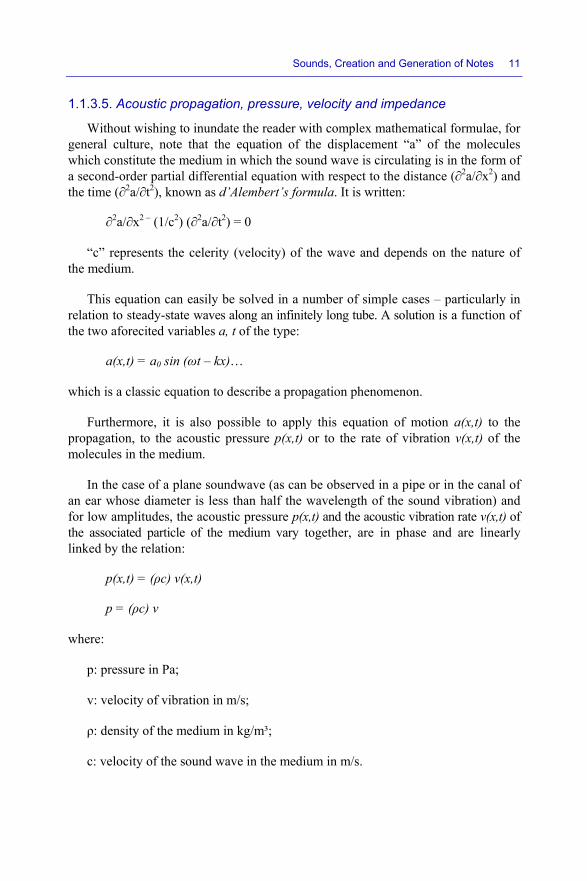
1.1.3.5. Acoustic propagation, pressure, velocity and impedance
Without wishing to inundate the reader with complex mathematical formulae, for general culture, note that the equation of the displacement “a” of the molecules which constitute the medium in which the sound wave is circulating is in the form of a second-order partial differential equation with respect to the distance (∂2a/∂x2) and the time (∂2a/∂t2), known as d’Alembert’s formula. It is written:
∂2a/∂x2 – (1/c2) (∂2a/∂t2) = 0
“c” represents the celerity (velocity) of the wave and depends on the nature of the medium.
This equation can easily be solved in a number of simple cases – particularly in relation to steady-state waves along an infinitely long tube. A solution is a function of the two aforecited variables a, t of the type:
a(x,t) = a0 sin (ωt – kx)…
which is a classic equation to describe a propagation phenomenon.
Furthermore, it is also possible to apply this equation of motion a(x,t) to the propagation, to the acoustic pressure p(x,t) or to the rate of vibration v(x,t) of the molecules in the medium.
In the case of a plane soundwave (as can be observed in a pipe or in the canal of an ear whose diameter is less than half the wavelength of the sound vibration) and for low amplitudes, the acoustic pressure p(x,t) and the acoustic vibration rate v(x,t) of the associated particle of the medium vary together, are in phase and are linearly linked by the relation:
p(x,t) = (ρc) v(x,t)
p = (ρc) v
where:
p: pressure in Pa;
v: velocity of vibration in m/s;
ρ: density of the medium in kg/m³;
c: velocity of the sound wave in the medium in m/s.
12 Musical Techniques
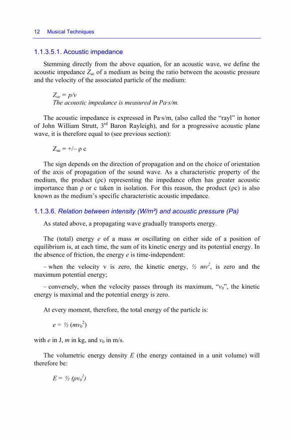
1.1.3.5.1. Acoustic impedance
Stemming directly from the above equation, for an acoustic wave, we define the acoustic impedance Zac of a medium as being the ratio between the acoustic pressure and the velocity of the associated particle of the medium:
Zac = p/v The acoustic impedance is measured in Pa·s/m.
The acoustic impedance is expressed in Pa·s/m, (also called the “rayl” in honor of John William Strutt, 3rd Baron Rayleigh), and for a progressive acoustic plane wave, it is therefore equal to (see previous section):
Zac = +/– ρ c
The sign depends on the direction of propagation and on the choice of orientation of the axis of propagation of the sound wave. As a characteristic property of the medium, the product (ρc) representing the impedance often has greater acoustic importance than ρ or c taken in isolation. For this reason, the product (ρc) is also known as the medium’s specific characteristic acoustic impedance.
1.1.3.6. Relation between intensity (W/m²) and acoustic pressure (Pa)
As stated above, a propagating wave gradually transports energy.
The (total) energy e of a mass m oscillating on either side of a position of equilibrium is, at each time, the sum of its kinetic energy and its potential energy. In the absence of friction, the energy e is time-independent:
– when the velocity v is zero, the kinetic energy, ½ mv2, is zero and the maximum potential energy;
– conversely, when the velocity passes through its maximum, “v0”, the kinetic energy is maximal and the potential energy is zero.
At every moment, therefore, the total energy of the particle is:
e = ½ (mv02)
with e in J, m in kg, and v0 in m/s.
The volumetric energy density E (the energy contained in a unit volume) will therefore be:
E = ½ (ρv02)

Sounds, Creation and Generation of Notes 13
where ρ is the mass per unit volume = density of the medium in kg/m³.
However, the energy contained in the wave propagates with a celerity c. As shown by Figure 1.4, we can deduce that the “total energy” E which, over the “unit time” Δt, crosses the “unit surface” S (called the surface power or acoustic intensity, I) is the energy contained in a volume whose base has a unit surface and whose height is equal to c.
Figure 1.4. Graphical representation of the acoustic intensity. For a color version of this figure, please
see www.iste.co.uk/paret/musical.zip
From this, by definition, it follows that:
I = (E /Δt) / S) = Pow / S, acoustic intensity in W/m²
I = cE = ½ (ρcv02)
I = (ρcv02) / 2
Taking account of the following (see above):
p = (ρc) v0
“I” can be expressed in the following better-known form:
I = p0²/2ρc
The total amount of sound energy J delivered to the tissues by a sonic irradiation over a time-period Δt is therefore:
J = I Δt

14 Musical Techniques
The pressure is a force per unit surface which is exerted on a mass: that of the neighboring element, and endows it with an acceleration – i.e. a variation in velocity.
In the conditions set out in the above paragraphs, we can show that at a certain point in space, the acoustic intensity I is linked to the acoustic pressure by the relation:
I = p² / ρ0c
in W/m², where:
– p: acoustic pressure in Pa;
– ρ0: density of the medium (in air, ρ0 ≃ 1.2 kg/m3 in normal conditions of temperature, humidity and atmospheric pressure);
– c: celerity (velocity) of sound and c = 340 m/s in the same conditions;
Thus:
I ≈ p² / 400
in W/m², with p in Pa.
NOTE.– In free space, the waves are not flat-fronted, but spherical, and the pressure and velocity do not vary exactly with one another. However, the more the radius of the sphere grows, the more the wave resembles a plane wave. The calculations with sine waves show that when the distance to the source is greater than or equal to the wavelength, we can assimilate the spherical wave to a plane wave.
NOTE.– This relation is valid only for direct sound coming from an acoustic source; not for sound reflected or echoed in a room.
1.1.3.6.1. Hearing- and pain thresholds
Whilst this may seem a little out of our field of study, let us say a few words about these two thresholds; in a few paragraphs, their relevance will become apparent, with the phenomena of masking as they also relate to concepts in harmony.

Sounds, Creation and Generation of Notes 15
Hearing threshold
The hearing threshold corresponds to the weakest sound (in terms of intensity) than an “average” ear is capable of perceiving. It corresponds to a mechanical vibration of the eardrum of around 0.3×10⁻¹⁰ m, which is minuscule.
At 1000 Hz, which is the frequency value commonly accepted for that referential hearing threshold, the corresponding acoustic pressure is:
p_ref = 2×10⁻⁵ Pa = 20µ Pa
In the knowledge that I = p²/ρ0c (in W/m2), the hearing threshold corresponds to a sound intensity of:
I_ref = 1×10⁻¹² W/m2 = 1 pW/m², i.e. 0dB(A)
Pain threshold
The value of the pain threshold corresponds to the acoustic pressure with maximum intensity that the “average” ear can withstand without being damaged. The commonly accepted value is:
p_pain = 20 Pa
Knowing that I = p²/ρ0c in W/m2, the pain threshold corresponds to a sound intensity of:
I_pain = 1 W/m2, which is 120 dB(A)
Thus, the ear has a dynamic (operational range) of around 120 dB (corresponding to acoustic intensities from 1 pW/m² to 1 W/m²).
1.1.3.7. Fletcher–Munson curve
Now that all these units are clearly defined, we can go beyond the physics and the beautiful mathematics and examine the hearing of a sustained sound. In this case, the human ear has specific characteristics that are summarized by the Fletcher–Munson curve / diagram (see Figure 1.5), which constitutes the auditory apparatus’ response to the stimulus of frequency as a function of the power emitted.

16 Mus
This human ehearing lwhich co120 decifrequencsensitivitknown tindividu
In ththis diffethat diagcritical) cit is/will or at ransuccessiorelations of their f
1.1.4. Id
Onceetc.) of t
sical Techniques
Figure 1version of th
figure shows ear as a functlies between torresponds to ibels). Furthecies and arounty of the ear that these limal, as a functio
he frequency rers from individgram (but for thcan be assimilbe easy to gen
ndom – or indon of those (physical valu
frequencies. W
dea of minim
e again, the inthe ear and of
s
1.5. Fletcher–Mhis figure, plea
the curves oftion of the frthe hearing thra sound inten
ermore, this hnd 15,000 Hz fis greatest in
mits vary fromon of his/her a
range audibledual to individhe time being,lated, simplistinerate “notes”
deed by defininfrequencies.
ues) with one aWe shall examin
mum audible
trinsic qualitiethe whole aud
Munson diagrase see www.i
f equal sound requency and reshold taken sity of 10-12 W
hearing range for high frequa range betw
m one subjectage or disease
e by the ear (tdual), any audi, the influenceically, for nowby creating a
ng a particularNonetheless,
another, particune this in detail
e gap/interv
es (mechanicaditory apparat
ram / curve. Foiste.co.uk/pare
sensations ofindicates thaas a reference
W/m²) and the is limited to
uencies. In addween around 1t to another, es and acciden
typically rougible “frequencye of amplitudew, to a “note”.
succession of r or specific mthese “notes
ularly in terms l in subsequent
val between
al – eardrums,tus are involve
or a color et/musical.zip
f a normal, funat the range oe (i.e. 0 dB at pain thresholdaround 30 H
dition, it show1 and 5 kHz. and even in
nts.
ghly 20-20,00y/amplitude” c
e is not consideOn principle, frequencies –
mode of creatis” may have
of the respectit chapters.
two frequen
, physiologicaed.
nctioning of normal 1000 Hz, d (around
Hz at low ws that the
It is well the same
0 Hz, but couple on ered to be therefore, arbitrarily ion of the
physical ive values
ncies
al – brain,

Sounds, Creation and Generation of Notes 17
1.1.4.1. Acoustic frequency resolution
Indeed, before going further, it is necessary and important to quantify – physically and physiologically (measure/define) – what might be the frequency resolution of an “average” ear; in other words, its auditory separation ability – i.e. which is the smallest frequency gap with which it is capable is distinguishing between two nearby frequencies.
We can show that the acoustic resolution of the human auditory apparatus depends on numerous factors. Among the main ones, we can cite:
– the absolute and relative acoustic levels at which the two frequencies involved are perceived;
– the presence or absence of neighboring frequencies of large amplitudes (see below):
- either simultaneous (frequency masking effect);
- or slightly shifted in time (temporal masking effect);
– the type of modeling of the psycho-acoustic apparatus;
– phenomena and definitions of consonance and dissonance, and of harshness, which we shall discuss in detail in Chapter 5;
– etc.
In conclusion, let us simply state that there comes a time when the ear is no longer able to distinguish between two close frequencies.
To clarify, let us also state that an average ear is able to quite easily distinguish between over thirty frequencies with the range of an octave (from f1 to 2×f1 – see below). Therefore, should we choose to use it, this minimum gap could represent the smallest frequency gap between two successive notes.
NOTE.– Physicists/acoustics experts, for their part, have long been able to divide the octave into 301 values, each one representing a “savart” (see Chapters 4 and 5). Thus, human frequency resolution corresponds to around 10 savarts, or slightly less. Certain animals perform far better than we do in this area.
Let us go into a little more detail about all this.
As previously noted, it has long been known that the ear has maximum sensitivity in the frequency range between around 1 and 5 kHz. In addition, the
18 Musical Techniques
sensitivity curves in the Fletcher–Munson diagrams represent the audibility threshold of a signal “A” as a function of its frequency in the absence of an “interference” signal if that interference is audible because it is above the perception threshold (see Figure 1.5, again). The question which then arises is: what happens when two signals are separated by a brief time lag, or are present simultaneously.
1.1.4.1.1. Static (in sustained sounds, of constant amplitudes but separated by a time lag)
In this case, the auditory apparatus (including the memory) must determine whether, at a given amplitude, one frequency is different or equal to another by successively switching between the two and listening to them one after the other. This gives an initial idea of the concepts of consonance and dissonance and of static frequency resolution of the auditory apparatus.
1.1.4.1.2. Dynamic: masking (in simultaneous sustained sounds of constant amplitudes)
Here, we enter into the zone of masking.
The concept of sound masking is closely linked to: the perception of a sound’s acoustic intensity; that of its frequencies (pitches), which we looked at in the sector on the physiology of the cochlea (notably with the outer hair cells); and to an auditory “channel” (i.e. a fiber in the auditory nerve) which responds only to a stimulus situated in a precise frequency range. This is what is known as the ear’s frequency selectivity.
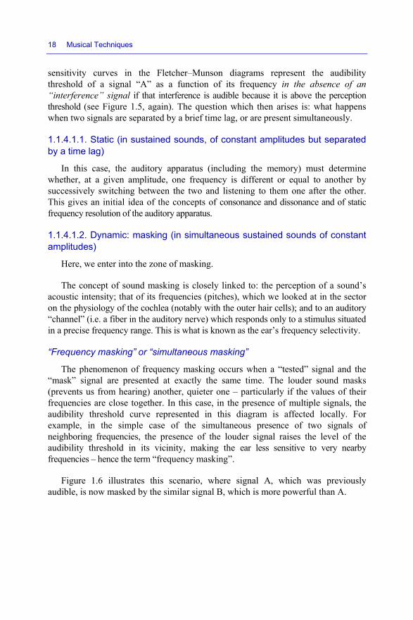
“Frequency masking” or “simultaneous masking”
The phenomenon of frequency masking occurs when a “tested” signal and the “mask” signal are presented at exactly the same time. The louder sound masks (prevents us from hearing) another, quieter one – particularly if the values of their frequencies are close together. In this case, in the presence of multiple signals, the audibility threshold curve represented in this diagram is affected locally. For example, in the simple case of the simultaneous presence of two signals of neighboring frequencies, the presence of the louder signal raises the level of the audibility threshold in its vicinity, making the ear less sensitive to very nearby frequencies – hence the term “frequency masking”.
Figure 1.6 illustrates this scenario, where signal A, which was previously audible, is now masked by the similar signal B, which is more powerful than A.

Sounds, Creation and Generation of Notes 19
Figure 1.6. Auditory impact of a loud signal B on a quiet similar signal A
This frequency selectivity is measured using objective tests and gives the neural tuning curves. These tuning curves show the detail of these masking phenomena.
“Temporal masking” or “sequential masking”
There is also another type of masking, known as “temporal masking”. This occurs when a high-amplitude sound masks weaker sounds that come immediately before or after it. Such masking takes place, in certain conditions, between two sounds which are not simultaneous, but instead are separated by a brief interval (e.g. the sound of a triangle immediately following the sound of a kettledrum). We then speak of temporal- or sequential masking, as opposed to the common case of frequency- or simultaneous masking discussed above.
Sequential masking manifests in short-term temporal interactions (spanning a few tens of a millisecond) between two stimuli/excitations. It is said to be:
– proactive, when the mask is presented before the test, meaning that the “mask” signal precedes the tested sound, which is also masked. This is the most significant case. It demonstrates mechanisms of inhibiting the excitability of the cochlea by way of an excitation immediately prior;
– retroactive, when the mask is presented after the test, meaning that the mask signal follows the tested sound, which is also masked. This masking, which could be described as “anti-causal” in signal processing, can only be explained as the interference of the temporal integration of these two competing signals.
Masking- and excitation patterns
To return to the subject that concerns us, in the Fletcher–Munson diagram, the zone/area of the “frequency/amplitude” plane in which another sound will no longer be perceived in the presence of the “mask” is known as the masking curve or “masking pattern” for that type of mask. The masking pattern of a pure sound or a narrowband sound exhibits a steep slope on the deeper-pitched side, and a gentler slope on the higher-pitched side. In this zone, therefore, masking is greater,

20 Mus
which caFigure 1
At thresponsefrequenccan be ascan be ebasilar mare involthe quietmasking hypothes
To qSOA (Stpresented
1.1.4.2.
Withforming charge o“MP3” acoustic called “pand a vathe frequthe sametheir twobasicallytriangle, psycho-a
sical Techniques
an be express.7).
Figu
he physiologice in the varcies. The envessimilated to th
explained (partmembrane, reilved. If it is strter sound, whpattern appro
sis has been co
quantify thesetimulus Onset d and the dura
Psycho-aco
hin the group the devoted “
of writing thesound encodimodel of hum
perceptual” enariable quantifuency institutie time, one mao frequencies ay empirical, b
drums, etc.)acoustic chara
s
sed by the sta
ure 1.7. Excita
cal level, the lrious auditoryelope of that rthe envelope otly) by selectiinforced by throng enough, hich is therefooximately coiorroborated b
phenomena, Asynchrony)
ation of the tim
oustic model
of experts – s“Audio” teame famous layeing. After nu
man hearing, wncoder. Such fication that iing, and if tway be perceiveare close togetbut fairly effe) engender noacteristics of t
atements “low
ation pattern an
oud sound or y channels nresponse cons
of the vibrationivity of the frhe active mechthe excitation ore “masked”incides with ty tests and ph
one of the p, which is the
me interval be
of human he
specialists in pm, the MPEG er III of the
umerous experwhich serves an encoder iss a function o
wo frequenciesed less than thther. This prinective. In thato perceptibleemporal mask
wer sounds m
nd masking pa
“mask” produnear to its stitutes its “excns of the basilrequency of thhanisms in whof the mask c
. This interprethe mask’s exhysiological ob
pertinent depee sum of the tifore the mask
earing
physiology, a(Moving PictMPEG 2 sta
riments, the gas the basis
s characterizeof the ear’s ses of different inhe other depennciple of modt percussive s pre-echo artking and “sub
mask higher on
attern
uces a greaterspecific frequcitation patternlar membranehe deformatiohich the outer covers that proetation impliexcitation pattebservations.
endent variablime at which t
k appears.
acoustics and pture Experts Gndard, well k
group chose aof the design
ed by a maskiensitivity in rentensities are
nding on whethdeling of our hsounds (such tifacts, it expband filtration
nes” (see
r or lesser uency or n”, which
e. Its form ons in the hair cells
oduced by s that the ern. This
les is the the test is
physics – Group) in known as a psycho-n of a so-ing curve elation to present at her or not hearing is as piano, ploits the n”, which

Sounds, Creation and Generation of Notes 21
consists of dividing the audio bandwidth (roughly 20-20,000 Hz) into 32 subbands of identical widths using an array of so-called “polyphase filters”. This is the principle of “perceptual audio coding”, which was chosen for compression into MP3 format to reduce the digital flowrate of information.
Following these highly scientific documentary points, we still need to make a number of additional comments before we can get back, in earnest, to what musicians expect from this book.
The audible band from 20 to 20,000 Hz, on principle, represents ten octaves, known as octave “0” to “9” (20 40 80 160 320 640 1280 2560 5120 10240 20480), which is often much too broad for a human being with a “typical” sense of hearing. In reality, humans typically only hear the eight main octaves indicated in italics here.
Additionally, in practice, the keyboard of an acoustic piano is usually made up of (81) 85 black and white keys (ranging from la0 (or A0) to la7), and that of digital pianos has 88 keys (from la0 to do8), which is slightly less than 8 octaves (see the example of the keyboard of a piano (Figure 1.8) and that of a conventional organ spans from fa2 = 87 Hz… la4 = 440 Hz… to do9 = 8372 Hz).
NOTE.– As we shall see later on, the white keys correspond to the seven notes in the diatonic scale of do major) (C) and the black keys to the five remaining notes needed to make up a chromatic scale – 12 notes per octave in total.
If we maximize, considering a keyboard with 8 octaves of 12 notes per octave, this makes a total of 96 notes. We then take an array of 32 filters: this gives us a group of 3 notes per filter, so a filter bandwidth of one-and-a-half tones = 3 semitones. Thus, it is on the basis of a 3-semitone interval that frequency masking is used in signal analysis.
NOTE.– In MPEG 3, the analog signal (the sound) output by a subband filter is then sampled. By processing that signal, we are able to eliminate the subband signals below the threshold (not perceived by the hearer) in the psycho-acoustic model, and defines the precision of quantification needed for each of the subbands, so that the quantification noise remains below the audibility threshold in that subband. In addition, the zones where the ear is most sensitive can therefore be quantified with greater precision than the others.

22 Musical Techniques
1.1.5. Why have we told this whole story, then?
That is a good question! The answer is simple: why both adding in harmonic elements or ornaments into a piece of music when no-one will hear them because of consonance, frequency- and/or temporal masking, etc. Thus, it is important to always pay attention to these latent phenomena.
We have finished, for the time being, with the physiological aspect, so let us now look at how notes are generated.
Figure 1.8. Usual range of frequencies on a piano keyboard

2
Generation of Notes
The aim of this chapter is to explain the long history through the ages (and therefore through the civilizations) which has led to the generation of musical notes and the definition of their frequencies (pitches/heights). Here again, there is a very close relationship between physics and music. Let us begin with the concept of an octave.
2.1. Concept of octave
During the creation of a particular series of frequencies (which have, in the past, and are, for the time being for simplicity of writing, called “notes”), it is possible that two of them will be linked by the fact that the frequency of one is double the value of the other. In this case, we say that they are spaced an octave apart.
octave = range of frequencies between “f” and “2f”
NOTE.– The word “octave” is, in principle, unfounded and completely inapt, and comes from the fact that, as we shall show in a number of chapters, for numerous reasons, double frequency corresponds to the “8th degree” of the well-known scale today; hence the name, octave.
This octave relation can, if we want, be repeated multiple times along an organized generation of series of frequencies.
If we call the first frequency (note) generated/encountered X0, also known as the fundamental or root, we look for the note with double the value of that frequency (i.e. an octave above), X1; then the frequency doubles again above X1 (i.e. two octaves above X0, so the frequency is four times that of X0), X2, etc. (see Table 2.1).
Musical Techniques: Frequencies and Harmony, First Edition. Dominique Paret and Serge Sibony. © ISTE Ltd 2017. Published by ISTE Ltd and John Wiley & Sons, Inc.

24 Musical Techniques
Frequency value … F0 2 × F0 4 × F0 8 × F0 …
Name of the note X0 X1 X2 X3
Number of octave “n” 0 1 2 3
Note 1 The “n” in “2n F0” represents what is usually called the rank of the octave.
For the mathematically minded
20 F0 21 F0 22 F0 23 F0
Note 2 The row for the “mathematically minded” here is only included to draw readers’ attention to a somewhat “logarithmic” aspect in the generation of the successive octaves, because this generation of octaves is based on an entity: “2 to the power of the octave number”. We shall come back to this later on.
Table 2.1. Relations between frequencies, octaves and octave ranks
The choice of whether or not there is an octave and multiple repetitions of 2 (or not) in a successive generation of frequencies (notes) is, in principle, purely arbitrary… However, we shall show later on that the mechanical-acoustic sensation thus created by the presence of these octaves is pleasant (a sort of unison) and that the human ear (i.e. the whole auditory system) is satisfied by that value. There are practically always frequencies spaced one or more octaves apart in a succession of “notes”.
2.1.1. Choice of inner division of an octave
Now supposing that we have, indeed, decided to include that idea of an octave in the progression of notes, we can then choose to define how the other notes between those two frequencies will (or could) be distributed.
Here, again, we have complete freedom. There are no rules of principle! To each musician his (or her) own…
This distribution may either be organized or be completely whimsical. Furthermore, again, in principle, there is no need to work with the same rules of distribution from one octave to the next. Let us be perfectly clear: the result obtained will reflect your own creativity… or your own cultures and civilizations!

Generation of Notes 25
Here, again, for numerous physiological reasons, our auditory apparatus, made up of the ear, its mechanical system, the associated operation of the brain (and thus sooner or later, our culture, our civilization) expresses sensations which often lead to a slightly greater organization.
This being the case, creating frequencies, dividing an octave into several pieces, distributing the frequencies is all very well, but how many pieces to use... That is the (major) question.
2.2. Modes of generation/creation/construction of notes
We have (for now!) concluded our little overview, in terms of the notions pertaining to frequencies, and have come to the crucial moment of the creation of a series of notes – i.e. the choice of frequencies to include in the interval that constitutes an octave from F to 2F.
All solutions can be envisaged:
– just for fun and to make readers smile, take (around) 30 audible values out of those discussed above, put them into a hat, draw them out at random and then attribute them a name. It is a very primitive exercise, but why not? Everyone can use their own method.
For centuries, every individual, every people, every civilization, every era has made its own small contribution to the work of creating and organizing the creation of the different frequencies that can be inserted within that famous “reference” octave. Hundreds of books have described this better than we could, but again, let us simply state that a number of thought-out “physical” and “physiological” manners can be envisaged for this.
Let us examine this new problem, in the knowledge that the outer and middle parts of our ear (look again at Figure 1.1) are wonderful mechanisms which are highly sensitive to variations in pressure, and like any mechanism, are sensitive to the well-known physical phenomena of “resonances” (a resonance consists of having significant reactions/variations in relation to a stimulus at varying frequencies but at a constant amplitude of excitation) – i.e. phenomena such as those which lead us now to discuss the contents and “harmonic” relations between the different frequencies presented to it.

26 Musical Techniques
2.3. Physical/natural generation of notes
2.3.1. Harmonics
For non-physicists (there is no shame in that; no-one is perfect!), know that the frequencies known as “harmonics“ are frequencies whose values are integer multiples (2F, 3F, 4F, 5F, etc.) of an original frequency F (preferably a pure sine wave), with that original being named the “fundamental frequency” (or, indeed, for some, first harmonics… when there are harmonics!) and simply written as “fundamental” (see the example in Figure 2.1).
Figure 2.1. Example of signals (top to bottom) at F, 2F and 3F
2.3.2. Fractional harmonics
Also note that somewhat bizarrely, we also use the terms “sub-harmonics” or “fractional harmonics” for the sub-multiples of harmonic frequencies – for example: F/2, F/3, 2F/3, 3F/4, 3F/5, 249F/521, etc. and also non-integer “overharmonics” 3F/2, 5F/2, 5F/3, etc. N.B. music is made up of precisely that (see Figure 2.2).
Figure 2.2. Example of signals (top to bottom) at F and F/3
Readcertain grequirem
Givewhose vwaves wfrequencywill be hintroducin the orTable 2.2
Number of the octave
0
1
2
3
ders now havegenerations ofments.
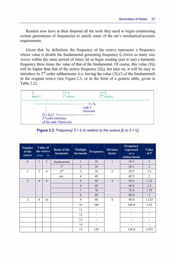
n that, by dealue is double
within the samy three times higher than thae its 2nd-orderriginal octave2).
Figure 2.3.
Value of the octave from to
R
1 2 fu
2 4
4 8
8 16
e at their dispf frequencies
efinition, the e the fundame
me period of tithe value of t
at of the octavr subharmonice (see Figure
Frequency 3
Rank of the harmonic
Mha
fundamental 1st 2nd etc.
osal all the toto satisfy som
frequency of ental generatinime), let us bethat of the funve frequency c (i.e. having t2.3, or in the
× f0 in relation
Multiple armonic Frequ
1 1F2 2F3 3F4 4F5 5F6 6F7 7F8 8F9 9F10 10F11 -12 -13 -14 -15 15F
ools they needme of the ear
f the octave rng frequency egin creating (ndamental. Of (2f0), but laterthe value (3f0)e form of a g
n to the octave
ency Division factor
F 1 F F 2 F F 4 F F F F 8 F
F
Generation of N
d to begin con’s mechanical
represents a ff0 (twice as m(just to see) a course, this vr on, it will b)/2 of the fundgeneric table,
e [f0 to 2 × f0]
Frequency expressed
as a subharmonic
1F/1 2F/1 3F/2 4F/2 5F/4 6F/4 7F/4 8F/4 9F/8 10F/8
- - - -
15F/8
Notes 27
nstructing l/acoustic
frequency many sine
harmonic value (3f0) be easy to damental)
given in
c
Value of F
1 2
1.5 2
1.25 1.5 1.75
2 1.125 1.25
- - - -
1.875

28 Musical Techniques
16 16F 16F/8 2
4 16 32 17 17F 16 17F/16 1.0625
18 18F 18F/16 1.125
19 - - -
20 20F 20F/16 1.25
… etc. etc. etc. etc.
Table 2.2. Frequencies expressed in subharmonics
To be perfectly clear, let us take an example (completely at random!), with:
f0 440 Hz, fundamental
2 × f0 880 Hz, 2nd harmonic or rank-1 harmonic
3 × f0 1320 Hz, 3rd harmonic or rank-2 harmonic
so:
3/2 × f0 660 Hz
This last frequency obtained (3/2 × f0 = 1.5F0) belongs to the interval [f0 – 2f0].
We have just shown how we obtained the “second” harmonic (3f0) of F0 (situated in the 2nd-rank octave). We propose to continue in the same way in relation to the other physical harmonics, by presenting them in the order of their apparition in the different octaves where they are situated (see Table 2.3).
Table 2.3. Table showing the successive orders of apparition of the integer harmonics in the different octaves. For a color version of
this table, please see www.iste.co.uk/paret/musical.zip

Generation of Notes 29
In this table, each row/range corresponds to an octave:
– octave from 1 to 2, known as the 0-order (or rank) octave;
– octave from 2 to 4, known as the 1st-order octave – i.e. (21) = 2;
– octave from 4 to 8, known as the 2nd-order octave – i.e. (22) = 4;
– octave from 8 to 16, known as the 3rd-order octave – i.e. (23) = 8;
– octave from 16 to 32, etc.;
– octave from 32 to 64, etc.
2.3.3. Initial conclusions
The last octave in the previous figure (multiples from 32 to 64) includes the presence of (too) numerous frequencies (or notes: 32 of them), which an average ear is often unable to completely discern (in this case, the ear’s frequency separating capacity may be surpassed, and hearing goes to the stage of “consonance”, “unison”, or “confusion” between certain frequencies, which we shall see in Chapter 5). As an initial approach and initial conclusion, we can say that in view of the “harmonic” process presented above, the maximum division of an octave could be that which stops at the end of the 5th octave, which exhibits only 16 frequencies to which it is therefore possible to assign specific names (see bibliography) – for example, see the set in Table 2.4:
Table 2.4. Table of succession of appearance of integer harmonics in the octaves. For a color version of this table, please see
www.iste.co.uk/paret/musical.zip
2.3.4. Order of appearance and initial naming of the notes
As Table 2.5 indicates, according to this process, the ascending order of appearance of the first 16 notes is as follows:

30 Musical Techniques
F0
Rank of the harmonic
1 2 3 4 5 6 7 8 9 10 11 12 13 14 15 16
Name attributed to the note
do1 do2 so2 do3 mi3 so3 pé3 do4 ré4 mi4 na4 so4 oc4 pé4 ti4 do5
Value in relation to [1, 2]
1/1 2/1 2
3/2 4/2 2
5/4 6/43/2
7/4 8/4 2
9/8 10/8 5/4
11/8 12/83/2
13/8 14/8 7/4
15/8 16/8 2
Table 2.5. Ascending order of appearance of the first 16 notes. For a color version of this table, please see www.iste.co.uk/paret/musical.zip
Once we have extracted, from this table, the values do2, do3, so3, do4, mi4, so4, pé4, do5, etc., which are exact multiples of the frequencies encountered above, out of the first eight values remaining, which we reclassify in ascending order of apparition in the interval [1, 2], we obtain eight values:
f0 × 1 do 1 1/1 = 8/8 9 ré 4 9/8
5 mi 3 5/4 = 10/8 11 na 4 11/8 = then situated in the fa# zone 3 so 2 3/2 = 12/8 13 oc 4 13/8 = then situated near to la 7 pé 3 7/4 = 14/8 = note situated between la3 and si3,
so almost a si3 flat 15 ti 4 15/8 = ti
This demonstrates that there are and will be direct, unavoidable physical harmonic relations, which our auditory apparatus can discern by pure relations of multiples and harmonic resonances, between the future notes do, so, mi, pé-ti flat, which are, in fact, the first harmonic frequencies encountered and which, with notations of particular ranges, would later become “thirds”, “fifths”, “sevenths”, etc. As if by a marvelous accident, they pay an important – predominant, even – role in “harmony”. Then come the harmonic frequencies whose ranks are immediately above, with slightly lesser influences in harmony, but which, later on, under the appellations of “9th, 11th and 13th”, would make their respective and relative contributions to the “color” of a chord.

Generation of Notes 31
Strange, is it not…?
Looking again at the last row in Table 2.4, we must work back to harmonic 32 (which is enormous!) to begin to see the appearance of the essence of the notes in a modern-day chromatic scale.
How bizarre, again…
F0
Rank of the harmonic
17 18 19 20 21 22 23 24 25 26 27 28 29 30 31 32
Name attributed to the note
do#5 ré5 re# mi5 fa na -
so5 so# oc la pé - ti - do6
Identical to fa#
Identical to la
Identical to ti b
Identical to ti
Value in relation to [1, 2]
17/16 18/16 9/8
19/16 20/16 5/4
21/16 22/1611/8
23/16 24/16 3/2
25/16 26/16 13/8
27/16 28/167/4
29/16 30/16 15/8
31/16 32/16 2
Table 2.6. Ascending order of apparition of the first chromatic notes. For a color version of this table, please see www.iste.co.uk/paret/musical.zip
Also note in both the last two figures:
– that the so appears first in this sequence (later on, it will act as a “fifth” in a conventional diatonic scale of seven notes), and that later, the name of “dominant“ note given to it may not be entirely without reason;
– that the mi appears next (it will later act as a “third” in a conventional 7-note diatonic scale), and this note will also have a very important role;
– finally, that the ti flat (written as ♭– bemolle) is not the first, but is not badly placed in the order of its appearance and that, as we shall see later on, the so-called “seventh” position (in actual fact, a minor seventh, in a conventional 12-note chromatic scale) is not bad at all.
Because octaves are obtained by doubling a frequency, we can, if we wish, express each of the notes corresponding to these harmonics as “sub-harmonics” (or “fractional harmonics”), within the first octave, to fit them into the primary octave (from 1F to 2F).

32 Musical Techniques
For example, this gives us:
– for the harmonic f3 in the 1st-order octave, a value = f3/(21) in the 0-rank octave;
– for the harmonic f9 in the 3rd-order octave, a value = f9/(23) in the 0-rank octave;
– etc.
Table 2.7. Comparisons and relative gaps between notes
Table 2.7 shows the result of the calculations relating to all these ratios and the relative gaps between these notes.
We have now completed what was a very hard task, which is already worth the effort, and in writing it, we have described the first type of note creation, with 16 notes per octave! What luxury!
2.3.5. A few important additional remarks
Purely out of sympathy for the reader, and so as not to go on for too long without concrete application, we have italicized these notes (giving their common names) that are closest to those which will ultimately be used often.

Generation of Notes 33
Also, in the right-hand column of this table, readers will find the relative gaps existing between two successive notes. Note that, along the length of the octave:
– the relative gap from note to note is not absolutely constant;
– the values of the gaps exhibit a certain amount of consistency;
– these values decrease regularly from the beginning of the octave towards the end;
– auditory perspective is undeniably “physical” in its construction, but perhaps not so easy (at a given date, in a given educational context and civilization, etc.) to learn, because the intervals are not entirely constant throughout the increase or decrease.
In fact, our ear does not work in terms of relative distance in linear mode, but in proportional mode, which means that it does not like linear additions, preferring products and divisions, or indeed it prefers additions and subtractions but only logarithms!
In brief, this “natural/physical” table will be extremely useful and will serve as the basis for comparison with all the other modes of generating a “note progression”, which we shall now construct differently.
Of the hundreds of possibilities for generating notes available to us, let us now look at new methods of constructing a succession of frequencies known as “pure perfect fifths”.
2.4. Generation of perfect fifth notes
The generation of so-called “perfect fifth” notes or the “Pythagorean” scale can be constructed in two possible ways: with the “ascending fifth” or the “descending fifth”.
2.4.1. Generation with ascending fifths
This sequence with “ascending fifth” is obtained by starting with an initial note of any frequency f0 (and sometimes, it is there that the trouble lies) and by multiplying that frequency by three (×3) and so on, little by little, going up in successive multiplication by “3” of the frequencies of the notes thus obtained. Here, some lucky readers may recall their school math classes on geometric progressions!
Why the word “fifth”, then, if we are speaking of three times the frequency (which, in reality, has no direct relation with the number “5”), and the term “fifth” or

34 Musical Techniques
ascending from “fifth to fifth”)? We shall see this later on: it is a good – even an excellent – question!
At the present point in this work, there is no explanation (because we do not yet officially know what the rest of this book holds), but – and there is always a but – we shall see a little later on that the frequency of the note (f0 × 3) expressed in the first octave corresponds to the fifth degree of the so-called major scale which everybody uses… Hence the name “fifth”! In fact, for the peace of mind of the purists among you, let us note that specifically, it is the fifth doubled into the higher octave.
Starting at f0, we successively obtain (3 f0), (9 f0), (27 f0), (81 f0), (243 f0), etc.: in brief, a series 3n, 1 < n < ∞ (see the red bold text in Table 2.8).
This, expressed in terms of values of sub-harmonics (by dividing by the appropriate values 2, 4, 8, 16…) in the reference first octave, gives us the following ratios – additionally reclassified in order… the luxury! (See Table 2.9).
The values in bold are those which are strictly identical to those obtained by the previous method of generation of notes by harmonic multiples (do, ré, so, la) whose fractional values are simple, and therefore consonant (and/or harmonics), but the others are not at all the same as those in the first generation. Certainly, they are close but they are different.
Table 2.8. Succession of occurrences of ascending fifths (3 f0), (9 f0), (27 f0), (81 f0), (243 f0), etc. For a color version of this table,
please see www.iste.co.uk/paret/musical.zip
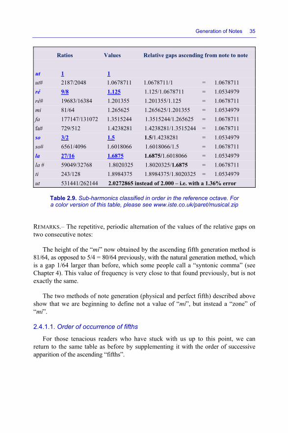
Generation of Notes 35
Ratios Values Relative gaps ascending from note to note ut 1 1 ut# 2187/2048 1.0678711 1.0678711/1 = 1.0678711 ré 9/8 1.125 1.125/1.0678711 = 1.0534979 ré# 19683/16384 1.201355 1.201355/1.125 = 1.0678711 mi 81/64 1.265625 1.265625/1.201355 = 1.0534979 fa 177147/131072 1.3515244 1.3515244/1.265625 = 1.0678711 fa# 729/512 1.4238281 1.4238281/1.3515244 = 1.0678711 so 3/2 1.5 1.5/1.4238281 = 1.0534979 so# 6561/4096 1.6018066 1.6018066/1.5 = 1.0678711 la 27/16 1.6875 1.6875/1.6018066 = 1.0534979 la # 59049/32768 1.8020325 1.8020325/1.6875 = 1.0678711 ti 243/128 1.8984375 1.8984375/1.8020325 = 1.0534979 ut 531441/262144 2.0272865 instead of 2.000 – i.e. with a 1.36% error
Table 2.9. Sub-harmonics classified in order in the reference octave. For a color version of this table, please see www.iste.co.uk/paret/musical.zip
REMARKS.– The repetitive, periodic alternation of the values of the relative gaps on two consecutive notes:
The height of the “mi” now obtained by the ascending fifth generation method is 81/64, as opposed to 5/4 = 80/64 previously, with the natural generation method, which is a gap 1/64 larger than before, which some people call a “syntonic comma” (see Chapter 4). This value of frequency is very close to that found previously, but is not exactly the same.
The two methods of note generation (physical and perfect fifth) described above show that we are beginning to define not a value of “mi”, but instead a “zone” of “mi”.
2.4.1.1. Order of occurrence of fifths
For those tenacious readers who have stuck with us up to this point, we can return to the same table as before by supplementing it with the order of successive apparition of the ascending “fifths”.

36 Musical Techniques
1 2
3 4 5 6 7 8 9 10 11
Table 2.10. Order of occurrence of ascending fifths
NOTE.–
a) The successive order of appearance of notes constructed to the perfect fifth is:
do0 → so1 ré2 la3 mi4 ti5…
As we shall see later on, in fact, this corresponds to the tone taking a sharp each time.
Tone of the major scale: so ré la mi ti ...
Number of sharps per key: 1 2 3 4 5
b) By the very principle of multiplication by 3, it is impossible to find an integer multiple of 2 of the original frequency! Thus, by ascending fifths generation, we shall never be able to find an even-numbered integer multiple (n × 2) of the fundamental frequency (the octave). This is demonstrated by the table, where we can see that the closest multiple of 3 to the first “do” (in relation to the origin) has the value:
312 = 531441 instead of 219 = 524288
which represents a ratio of 531441/524288 = 1.0136433
which represents a gap of 1.36433%, as previously stated.
Thus, rather than a “do”, we have more of a “D’Oh!”

Generation of Notes 37
2.4.2. Generation with descending fifths
Here is a new problem, which is corollary to the previous one.
We can also start with an initial frequency by doing likewise and dividing its value by 3, and so on, descending. It is the same pattern, backwards – hence the appellation “descending fifth”.
In summary, the value of the frequency of any given note is always the triple or a third of that of another note!
In short, there is/are (a) generation(s) to the ascending fifth and to the descending fifth and without any major problems we can therefore make a fifth out of anything!
The frequency f0 which we have chosen as a starting point is, itself, somewhere, the “double fifth”, the third-order multiple, of another frequency. Thus, we can construct the same table for descending fifths by successively dividing all the new frequencies obtained by three.
We obtain the “descending fifth” situated two octaves below F0 (see Table 2.11).
f0/16 f0/8 f0/4 f0/2 f0 f0/3 f0/9
Table 2.11. Order of succession of descending fifths. For a color version of this table, please see www.iste.co.uk/paret/musical.zip
Thus, expressed in relation to the reference octave, see Table 2.12.
f0 2 × f0 (4 × f0)/3 (16 × f0)/9
Table 2.12. Fifths expressed in the reference octave
In the same way as above, if readers give us their trust, Table 2.13 shows the order of appearance of the successive descending “fifths” when they are expressed in the reference octave.
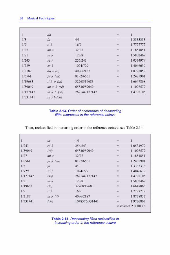
38 Musical Techniques
1 do = 1 1/3 fa 4/3 = 1.3333333 1/9 ti♭ 16/9 = 1.7777777 1/27 mi♭ 32/27 = 1.1851851 1/81 la♭ 128/81 = 1.5802469 1/243 ré♭ 256/243 = 1.0534979 1/729 so♭ 1024/729 = 1.4046639 1/2187 do♭ (ti) 4096/2187 = 1.8728852 1/6561 fa♭ (mi) 8192/6561 = 1.2485901 1/19683 ti♭♭ (la) 32768/19683 = 1.6647868 1/59049 mi♭♭ (ré) 65536/59049 = 1.1098579 1/177147 la♭♭ (so) 262144/177147 = 1.4798105 1/531441 ré♭b (do)
Table 2.13. Order of occurrence of descending fifths expressed in the reference octave
Then, reclassified in increasing order in the reference octave: see Table 2.14.
1 ut 1/1 = 1 1/243 ré♭ 256/243 = 1.0534979 1/59049 (ré) 65536/59049 = 1.1098579 1/27 mi♭ 32/27 = 1.1851851 1/6561 fa♭ (mi) 8192/6561 = 1.2485901 1/3 fa 4/3 = 1.3333333 1/729 so♭ 1024/729 = 1.4046639 1/177147 (so) 262144/177147 = 1.4798105 1/81 la♭ 128/81 = 1.5802469 1/19683 (la) 32768/19683 = 1.6647868 1/9 ti♭ 16/9 = 1.7777777 1/2187 ut♭ (ti) 4096/2187 = 1.8728852 1/531441 (do) 1048576/531441 = 1.9730807 instead of 2.000000!
Table 2.14. Descending fifths reclassified in increasing order in the reference octave
Generation of Notes 39
NOTE.–
a) The order of successive occurrence of the notes constructed to the fifth is:
do0 → fa ti♭ mi♭ la♭ ré♭ ...
As we shall see later on, this in fact corresponds to the tone with a flat each time:
Tone of the major scale : fa ti♭ mi♭ la♭ ré♭ ...
Number of flats in the key: 1 2 3 4 5
b) By the very principle of division by 3, it is impossible to find an integer multiple of 2 of the original frequency! Thus, by descending fifths generation, we shall never be able to find an even-numbered integer multiple (n × 2) of the fundamental frequency, which is demonstrated by the table, where we can see that the closest multiple of 3 to the first “do” per octave has the value:
1048576/531441 = 1.9730807
312 = 531441 instead of 219 = 524288
which is a gap of 531441/524288 = 1.0136433
This would no longer be a “do”, then, but a “re-D’oh!”
2.4.3. Conclusions on fifth-based constructions of notes
As shown by the two constructions of notes above “to the fifth”, the values obtained and expressed (“sub-” and “over-” harmonics, or indeed “fractional” harmonics) in the reference octave are not strictly identical.
Once again, many frequencies are close, but are not absolutely identical. Thus, there are generations to the fifth and to the fifth (ascending and descending fifths)! In addition, supposing we take, as the initial value, the “lock” do (the do in the central mechanical position on a piano keyboard) as the basis for the construction of ascending and descending fifths, with the fact that we shall never again find an exact do as we work our way up (3, 9, 27, 81… but never an even-numbered value), and that in this case the do must be the fifth of a lower note situated at 1/3, 1/9, 1/27… its frequency), and therefore that the ascending and descending fifths will, by their very principle, never yield the same notes expressed in a central octave. Therefore, when we speak of construction to the fifth:
– first, we must state the frequency (the note) at which we began;
– secondly, we must say whether the construction is performed with ascending or descending fifths.
40 Musical Techniques
2.5. Important remarks on “physical”/“fifths” generation
Whether it is “physical” note generation or “ascending and descending fifths” constructions, we obtain “zones” of “notes” in which the frequencies are close, which tends to give names (of “notes”) to these particular zones.
With these groups of three values, we can construct a comparative table, which shows that:
– there are zones of preferential frequencies due to these constructions;
– the number of different main zones thus constructed is 12;
– we may decide to name each of the particular zones of frequencies;
– the gaps from zone to zone are not necessarily equal (the gap is not constant), but seem to be fairly regular;
– for each zone, we can choose a single particular value if we wish, and assign it the name of the zone which contains it.
All other considerations aside, with all of these frequencies:
– we may also name the smallest interval thus created which separates two consecutive notes – for instance, calling it a “semitone” (which means that someone has already defined a “tone”!);
– we may decide (later) to make that relative gap (the semitone) constant (regular) by “tempering” it along an octave (as we shall see a little later on, in the next few sections on “twelfth root of two” – see generation of tempered notes).
Then, it is possible to construct, within an octave, in accordance with our own wishes, a string of notes (5, 6, 7, 8, 10, etc.) serving as a basis/reference – which we shall later call a “scale” – based on a specific choice of any given increasing dis-tribution based on these twelve main frequencies.
The best-known and most usual example is that which comes from a particular choice: the choice of the diatonic “major scale” of seven notes – “do ré mi fa so la ti do” – with assorted frequency gaps, which we shall see in the next chapter.
Thus, having chosen these notes, it becomes easy to quantify the gaps (intervals) between them.
2.6. Generation of tempered notes
It is possible to tune a piano simultaneously to the ascending fifth and the descending fifth, from a specific note, or else play two pianos: one tuned to ascending

Generation of Notes 41
fifths and the other to descending fifths… but there is a risk of nasty surprises in disparity of the sounding of notes (see previous paragraphs). Thus, in a few paragraphs, to remedy this problem, we mention the creation of tempered notes which, though totally artificial (“chemically pure”), is a correct solution, and contains notes whose frequencies are situated very close to the generations of notes by “natural” frequencies and by “fifths”.
2.6.1. Notion of the ear’s logarithmic sensitivity
Before discussing the way to generate notes in a tempered fashion, let us take a moment to look at the ear’s logarithmic sensitivity to frequency. Is this true or false?
– what is true is that (the mechanics of) the ear (like all mechanics) likes integer multiples or “harmonics” and physical fractionals of a base frequency (see the previous chapters). Therefore, when we speak of multiples, sooner or later we come back to the geometric progression of notions confining to logarithms.
– what is not true is that the previous paragraph is based on centuries of western education/civilization, where somewhere in our subconscious, we have been educated with (if not sometimes steeped in!) that organization of notes structured to the octave, to the fifth, etc. Once again, if we had lived for thousands of years in the Far East, out in the brush, etc., it is highly likely that our ear would have unconsciously picked up other harmonic references, and that the octave and fifth would not be what they are for us westerners. Perhaps, on the Cartesian side, the European Renaissance era and many other phenomena have occurred for a reason?
This being the case, to return to the generation of tempered notes, the question does not arise. So let’s draw a line under it, assume everybody is the same, and move on. Thus, by definition, we decide to impose the requirement that we generate twelve notes in an octave and a growth exponent “n” which is identical from note to note, as we move in both directions! More simply put, all intervals, hereafter referred to as “tones” and “semitones”, will respectively be equal in value, in both an upward and a downward direction!
What is the value “n” of the growth ratio? By definition, with an octave being defined by a frequency ratio whose value is equal to 2, we merely need to decide on the number of steps “n” we wish to have in the octave.
We shall show, over the course of the next few chapters, that the ear is satisfied with 10 to around 25 steps per octave, and the above paragraphs have shown that 12 zones of notes was a reasonable number, so why not go with 12?

42 Musical Techniques
If we decide to evenly distribute twelve steps (notes) logarithmically spaced throughout the octave, this gives us:
– either:
F0 × n × n × n × ... 12 times over = (n12) × F0 = 2 × F0
– or:
n12 = 2
– or indeed:
n = 12th root of 2 = 1.0546307...
What a wonder (and also somewhat deliberate too!) – this value is very close to the note gap obtained by the fifths methods, so close to the notes created by many existing instruments. With that, music and electronic circuitry move forward!
NOTE.– Our (western) ear is now satisfied, the hairs of the auditory apparatus having been stroked in the direction of growth. However, true “harmonic” harmony – in the sense of organ pipes (which resonate physically and mechanically), of horns, bugles, etc. which vibrate (where there is little or no possibility of changing the heights of the notes!), guitar strings which vibrate (the height/frequency of the sound is largely mechanically predetermined by the position of the fret), but not violins, cellos, trombones, etc. which, for their part, allow the player to “create the height of the sounds” as s/he wishes, by positioning the fingers or hands wherever s/he chooses.
This being the case, we shall also show, during the next few chapters, that this singular distribution presents a significant advantage: the ability to transpose music in either direction!
ut = 1 ut# = ut#/ut = 1.05946307 = 1.05946307 ré ré/ut# = 1.05946307 = 1.1224618 ré# etc. = 1.05946307 = 1.1892068 mi = 1.05946307 = 1.2599206 fa = 1.05946307 = 1.3348393 fa# = 1.05946307 = 1.4142128 so = 1.05946307 = 1.4983061 so # = 1.05946307 = 1.5873999 la = 1.05946307 = 1.6817915 la# = 1.05946307 = 1.7817958 ti = 1.05946307 = 1.8877468 do = 1.05946307 = 2.0000000
Table 2.15. Distribution of frequencies of a generation of tempered notes

Generation of Notes 43
NOTE.– On western tastes (Europe, USA, etc.) as opposed to oriental tastes. Unlike in eastern cultures, it is normal that the values attributed to the harmonics, other than those of even-numbered orders (the successive octaves) should be incorrect, because western music is mainly structured around so-called tempered dodecaphony, which (as we shall see later) means that the ratio between the frequencies of two successive notes (a semitone) is constant and equal to the 12th root of 2. Thus, the harmonic 3, in a tempered scale, has the value of 219/12 = 2.9966 (instead of 3); the harmonic 5 = 228/12 = 5.039684 (instead of 5); and so on.
NOTE.– How can we tune a piano like that without a reference and a “pitch-perfect” ear to within 1/10 of a Hertz (i.e. a genuine frequency meter)? This is a good question! To the octave or to the fifth was somewhat easier, was it not?
2.6.2. Examples of electronic generation of tempered notes
In order to simplify electronic circuitry and to decrease the cost and maintenance requirements of the device (the instrument) – notably in terms of its tuning (or retuning), most electronic instrument manufacturers build in a master oscillator working at a very high frequency (several megahertz) so as to be able to divide the value of its frequency by appropriate factors capable of generating the successions of notes of the highest tempered octave the instrument is able to produce with the greatest possible precision. This technique poses the problem of defining the values of the division factors which we have after the master oscillator, and hence the “trueness” and accuracy of the notes thus created.
How are we to choose these values? The answer is simple, and is based on two contradictory criteria:
– the successive values of all the quotients must be as close as possible to the 12th root of 2;
– for basically technological and economic reasons, the value of the frequency of the master oscillator must be as low as possible, and thus the values of the dividers must be integers and as small as possible.
2.6.3. Relative gaps between tempered and electronic notes
By way of example, let us give the division factors which were (and indeed still are) commonly employed by the integrated circuit manufacturers National

44 Musical Techniques
Semiconductors NS, AMI, Yamaha, etc., to cite only a few of the oldest and best-known names (see Table 2.16).
Values of division factors of the master oscillator
f0 : 478 i.e.: = 1 451 478/451 = 1.0598669 426 478/426 = 1.1220657 402 478/402 = 1.1890547 379 478/379 = 1.2612137 358 478/358 = 1.3351955 338 478/338 = 1.4142011 319 478/319 = 1.4984326 301 478/301 = 1.5880398 284 478/284 = 1.6830985 268 478/268 = 1.783582 253 478/253 = 1.889328 239 478/239 = 2
Table 2.16. Typical values of division factors used by the master oscillator
In this table, the most critical ratio for finding the height of the note is the very first one: 478/451. Obviously, the higher the numerator, the greater the chance of finding an integer quotient which is close to the 12th root of 2. On the other hand, the higher the value of the numerator, the higher the frequency of the master oscillator will need to be.
EXAMPLE.– If we suppose that the frequency of the highest note we want to create is a do 10, which is around 16,000 Hz, then the master oscillator must oscillate at least at: 478 × 16,000 Hz, which is around 8 MHz.
For the other ratios, it is always easy to find the most appropriate value within the chain of dividers.
Figure 2.4 is a photocopy of the old conventional diagram of a top-of-the-range electronic organ (but not a Hammond organ, in which the notes are generated electro-mechanically by phonic wheels). Highlighted in the diagram is the master oscillator and all the dividers serving to generate the notes.

Generation of Notes 45
Figure 2.4. Diagram of a master oscillator and frequency dividers associated with a top-of-the-range electronic organ (document from Lowrey). For a color version of this figure, please see www.iste.co.uk/paret/musical.zip
We shall leave the description of different methods of generating “notes” here, but readers must have realized that there may be dozens of other methods, and now understand the difficulty, sometimes, of playing horns, guitars, pipe organs, electronic organs and ancient instruments all together. Good luck, and enjoy the music!
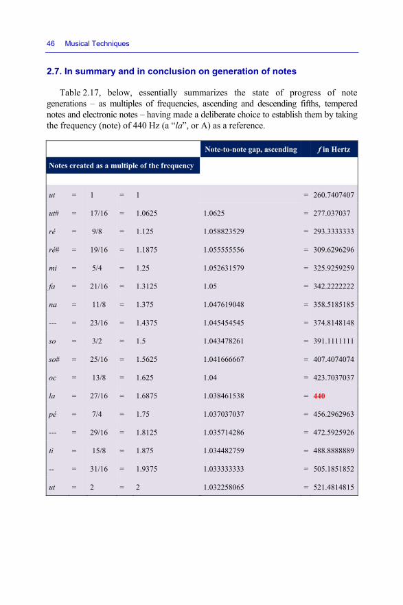
46 Musical Techniques
2.7. In summary and in conclusion on generation of notes
Table 2.17, below, essentially summarizes the state of progress of note generations – as multiples of frequencies, ascending and descending fifths, tempered notes and electronic notes – having made a deliberate choice to establish them by taking the frequency (note) of 440 Hz (a “la”, or A) as a reference.
Note-to-note gap, ascending f in Hertz
Notes created as a multiple of the frequency
ut = 1 = 1 = 260.7407407
ut# = 17/16 = 1.0625 1.0625 = 277.037037
ré = 9/8 = 1.125 1.058823529 = 293.3333333
ré# = 19/16 = 1.1875 1.055555556 = 309.6296296
mi = 5/4 = 1.25 1.052631579 = 325.9259259
fa = 21/16 = 1.3125 1.05 = 342.2222222
na = 11/8 = 1.375 1.047619048 = 358.5185185
--- = 23/16 = 1.4375 1.045454545 = 374.8148148
so = 3/2 = 1.5 1.043478261 = 391.1111111
so# = 25/16 = 1.5625 1.041666667 = 407.4074074
oc = 13/8 = 1.625 1.04 = 423.7037037
la = 27/16 = 1.6875 1.038461538 = 440
pé = 7/4 = 1.75 1.037037037 = 456.2962963
--- = 29/16 = 1.8125 1.035714286 = 472.5925926
ti = 15/8 = 1.875 1.034482759 = 488.8888889
-- = 31/16 = 1.9375 1.033333333 = 505.1851852
ut = 2 = 2 1.032258065 = 521.4814815

Generation of Notes 47
Notes created as ascending fifths
ut = 1 = 1 260.7407407
ut# = 2187/2048 = 1.0678711 = 1.0678711 = 278.4375016
ré = 9/8 = 1.125 = 1.053497936 = 293.3333333
ré# = 19683/16384 = 1.201355 = 1.067871111 = 313.2421926
mi = 81/64 = 1.265625 = 1.053497925 = 330
fa = 177147/131072 = 1.3515244 = 1.067871131 = 352.3974732
fa# = 729/512 = 1.4238281 = 1.053497887 = 371.2499935
so = 3/2 = 1.5 = 1.053497961 = 391.1111111
so# = 6561/4096 = 1.6018066 = 1.067871067 = 417.6562394
la = 27/16 = 1.6875 = 1.053497969 = 440
la # = 59049/32768 = 1.8020325 = 1.067871111 = 469.8632889
ti = 243/128 = 1.8984375 = 1.053497925 = 495
ut = 531441/262144 = 2.0272865 1.067871078 = 528.5961837 instead of 2.000000
Notes created as descending fifth
ut = 1/1 = 1 264.2981071
ré♭ = 256/243 = 1.0534979 1.0534979 278.4375008
(ré) = 65536/59049 = 1.1098579 1.053497971 293.3333421
mi♭ = 32/27 = 1.1851851 1.067871031 313.2421785
fa♭ (mi) = 8192/6561 = 1.2485901 1.053497973 330
fa = 4/3 = 1.3333333 1.067871113 352.3974674
so♭ = 1024/729 = 1.4046639 1.053497951 371.2500099
(so) = 262144/177147 = 1.4798105 1.053497922 391.111114
la♭ = 128/81 = 1.5802469 1.067871123 417.6562645
(la) = 32768/19683 = 1.6647868 1.053497906 440
ti♭ = 16/9 = 1.7777777 1.067871093 469.863281
ut♭ (ti) = 4096/2187 = 1.8728852 1.053497971 495.0000132
(ut) = 1048576/531441 = 1.9730807 1.05349794 521.4814942 instead of 2.000000 !

48 Musical Techniques
Tempered notes
ut 1 = 261.6257723 ut# = ut #/ut = 1.05946307 = 1.05946307 277.1828439 ré = ré/ut# = 1.1224618 = 1.05946307 = 293.6649353 ré# = = 1.1892068 = 1.05946307 = 311.1271474 mi = = 1.2599206 = 1.05946307 = 329.6277 fa = = 1.3348393 = 1.05946307 = 349.2283627 fa# = = 1.4142128 = 1.05946307 = 369.994516 so = = 1.4983061 = 1.05946307 = 391.9954905 so # = = 1.5873999 = 1.05946307 = 415.3047248 la = = 1.6817915 = 1.05946307 = 440 la# = = 1.7817958 = 1.05946307 = 466.1637022 ti = = 1.8877468 = 1.05946307 = 493.8832144 do = = 2 = 1.05946307 = 523.2515446
“Electronic” notes
Values of division factors ut 478/478 = 1 = = 261.4226084 ut# 478/451 = 1.0598669 = 1.0598669 = 277.0731695 ré 478/426 = 1.1220657 = 1.058685482 = 293.333342 ré# 478/402 = 1.1890547 = 1.059701495 = 310.8457812 mi 478/379 = 1.2612137 = 1.060686022 = 329.7097752 fa 478/358 = 1.3351955 = 1.058659211 = 349.0502903 fa# 478/338 = 1.4142011 = 1.05917156 = 369.7041403 so 478/319 = 1.4984326 = 1.05956119 = 391.7241587 so # 478/301 = 1.5880398 = 1.059800621 = 415.1495067 la 478/284 = 1.6830985 = 1.059859142 = 440 la# 478/268 = 1.783582 = 1.059701497 = 466.2686587 ti 478/253 = 1.889328 = 1.059288555 = 493.9130538 do 478/239 = 2 = 1.058577441 = 522.8452167
Table 2.17. Summary of generations of frequencies/notes – by multiples of frequencies, ascending and descending
fifths, tempered notes and in electronics
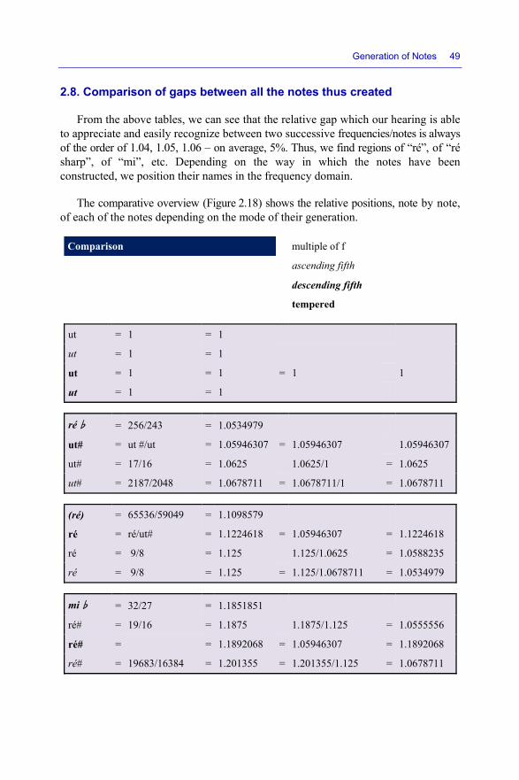
Generation of Notes 49
2.8. Comparison of gaps between all the notes thus created
From the above tables, we can see that the relative gap which our hearing is able to appreciate and easily recognize between two successive frequencies/notes is always of the order of 1.04, 1.05, 1.06 – on average, 5%. Thus, we find regions of “ré”, of “ré sharp”, of “mi”, etc. Depending on the way in which the notes have been constructed, we position their names in the frequency domain.
The comparative overview (Figure 2.18) shows the relative positions, note by note, of each of the notes depending on the mode of their generation.
Comparison multiple of f
ascending fifth
descending fifth
tempered
ut = 1 = 1
ut = 1 = 1
ut = 1 = 1 = 1 1
ut = 1 = 1
ré♭ = 256/243 = 1.0534979
ut# = ut #/ut = 1.05946307 = 1.05946307 1.05946307
ut# = 17/16 = 1.0625 1.0625/1 = 1.0625
ut# = 2187/2048 = 1.0678711 = 1.0678711/1 = 1.0678711
(ré) = 65536/59049 = 1.1098579
ré = ré/ut# = 1.1224618 = 1.05946307 = 1.1224618
ré = 9/8 = 1.125 1.125/1.0625 = 1.0588235
ré = 9/8 = 1.125 = 1.125/1.0678711 = 1.0534979
mi♭ = 32/27 = 1.1851851
ré# = 19/16 = 1.1875 1.1875/1.125 = 1.0555556
ré# = = 1.1892068 = 1.05946307 = 1.1892068
ré# = 19683/16384 = 1.201355 = 1.201355/1.125 = 1.0678711

50 Musical Techniques
fa♭ (mi) = 8192/6561 = 1.2485901 mi = 5/4 = 1.25 1.25/1.1875 = 1.0526316 mi = = 1.2599206 = 1.05946307 = 1.2599206 mi = 81/64 = 1.265625 = 1.265625/1.201355 = 1.0534979
fa = 21/16 = 1.3125 1.3125/1.25 = 1.05 fa = 4/3 = 1.3333333 fa = = 1.3348393 = 1.05946307 = 1.3348393 fa = 177147/131072 = 1.3515244 = 1.3515244/1.265625 = 1.0678711
na = 11/8 = 1.375 1.375/1.3125 = 1.047619
so♭ = 1024/729 = 1.4046639 fa# = = 1.4142128 = 1.05946307 = 1.4142128 fa# = 729/512 = 1.4238281 = 1.4238281/1.3515244 =
--- = 23/16 = 1.4375 1.4375/1.375 = 1.0454545
(so) = 262144/177147 = 1.4798105 so = = 1.4983061 = 1.05946307 = 1.4983061 so = 3/2 = 1.5 1.5/1.4375 = 1.0434783 so = 3/2 = 1.5 = =
so# = 25/16 = 1.5625 1.5625/1.5 = 1.0416667
la♭ = 128/81 = 1.5802469 so # = = 1.5873999 = 1.05946307 = 1.5873999 so# = 6561/4096 = 1.6018066 = =
oc = 13/8 = 1.625 1.625/1.5625 = 1.04
(la) = 32768/19683 = 1.6647868 la = = 1.6817915 = 1.05946307 = 1.6817915 la = 27/16 = 1.6875 1.6875/1.625 = 1.0384615 la = 27/16 = 1.6875 = =
pé = 7/4 = 1.75 1.75/1.6875 = 1.037037
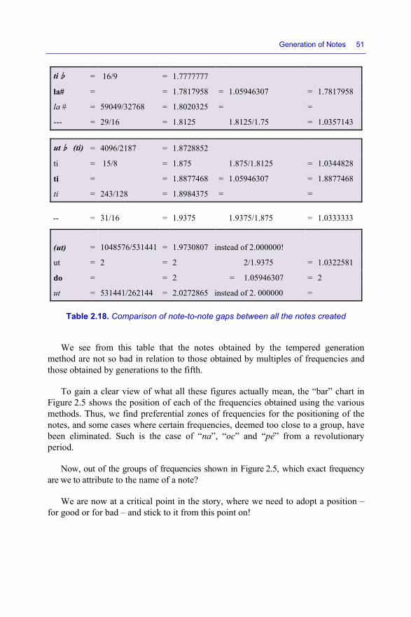
Generation of Notes 51
ti♭ = 16/9 = 1.7777777
la# = = 1.7817958 = 1.05946307 = 1.7817958
la # = 59049/32768 = 1.8020325 = =
--- = 29/16 = 1.8125 1.8125/1.75 = 1.0357143
ut♭ (ti) = 4096/2187 = 1.8728852
ti = 15/8 = 1.875 1.875/1.8125 = 1.0344828
ti = = 1.8877468 = 1.05946307 = 1.8877468
ti = 243/128 = 1.8984375 = =
-- = 31/16 = 1.9375 1.9375/1.875 = 1.0333333
(ut) = 1048576/531441 = 1.9730807 instead of 2.000000!
ut = 2 = 2 2/1.9375 = 1.0322581
do = = 2 = 1.05946307 = 2
ut = 531441/262144 = 2.0272865 instead of 2. 000000 =
Table 2.18. Comparison of note-to-note gaps between all the notes created
We see from this table that the notes obtained by the tempered generation method are not so bad in relation to those obtained by multiples of frequencies and those obtained by generations to the fifth.
To gain a clear view of what all these figures actually mean, the “bar” chart in Figure 2.5 shows the position of each of the frequencies obtained using the various methods. Thus, we find preferential zones of frequencies for the positioning of the notes, and some cases where certain frequencies, deemed too close to a group, have been eliminated. Such is the case of “na”, “oc” and “pé” from a revolutionary period.
Now, out of the groups of frequencies shown in Figure 2.5, which exact frequency are we to attribute to the name of a note?
We are now at a critical point in the story, where we need to adopt a position – for good or for bad – and stick to it from this point on!
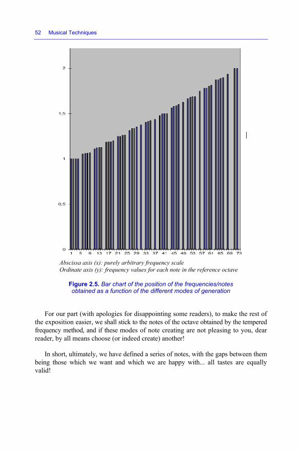
52 Mus
For othe expofrequencyreader, b
In shbeing thvalid!
sical Techniques
Abscissa axis (Ordinate axis
Figure 2.obtained
our part (with osition easier, y method, and
by all means c
hort, ultimatelyose which we
s
(x): purely arbi(y): frequency v
5. Bar chart od as a function
apologies forwe shall stick
d if these modhoose (or inde
y, we have defe want and w
itrary frequencyvalues for each
f the position n of the differen
r disappointinto the notes o
des of note creeed create) an
fined a series owhich we are
y scale h note in the refe
of the frequennt modes of g
g some readerf the octave obeating are not
nother!
of notes, with happy with...
ference octave
ncies/notes generation
rs), to make thbtained by the t pleasing to y
the gaps betw all tastes are
he rest of tempered
you, dear
ween them e equally

Generation of Notes 53
2.8.1. Note on pitch-perfect hearing… or is it?
How many times have we heard about someone who has a “pitch-perfect ear”? Being curious rather than credulous, we suggest running a little experiment.
2.8.1.1. Little experiment
– Take a “perfect ear” (and the biped who comes with it, of course).
– Play a mi3 on the keyboard of a piano.
– Wait for the verdict.
It is a mi3! Bravo! This is not easy to determine for mere mortals, but for numerous musicians, the test is fairly easy up to this point!
Getting more difficult now, ask the person which mi3 it is:
– is it a mi3 on a piano obtained when the instrument is tuned to the ascending fifth?
– is it a mi3 of a piano tuned to the descending fifth?
– from which base note are the fifths defined?
– is it a mi3 obtained on a piano tuned to the tempered scale?
For your pleasure, to define these notes to the exact hertz frequency, look again at Tables 2.17 and 2.18.
If the “ear” is still able to withstand the test:
– simultaneously play, on two synthesizers which are very slightly out of tune with one another, two mi3 notes a few savarts apart (3 to 5, for example – see the next chapters), so that, for any human being, the notes are practically consonant;
– then, in the confusion, cease playing one of the two mi3s whilst continuing to hold the other, and slyly, ask the person to identify the note continuing to sound. We recommend that you repeat the experiment several times, because probability theory, random chance and bluff mean the person has a one-in-two chance of indicating the correct result completely at random, totally undermining this whole construction!
If the result is always perfectly correct, the “pitch-perfect” person in question must, at birth, have assimilated a laboratory measuring device known as a “frequency meter” (see Figure 2.6), and must immediately be encased in glass at the Natural History Museum, because as yet, there have been no recorded examples, and you have the only one in existence, which will make you a fortune.

54 Musical Techniques
We, for our part, are still poor…
Figure 2.6. Example of a true “pitch-perfect ear” – a professional lab frequency meter (document from Keysight Agilent). For a color version
of this figure, please see www.iste.co.uk/paret/musical.zip
We have now completed our detour into the generation of notes and the physical and mathematical ratios existing between them, and can take a little rest.

3
Recreation: Frequencies, Sounds and Timbres
3.1. Differences between a pure frequency and the timbre of an instrument
From the very start of this book, in an incorrect use of language and in the spirit of deliberate simplification, we have made a certain amalgamation between the terms frequency, sound, note and timbre. It is now time to correct these mistakes, because there are subtle nuances between all of these terms. Indeed, up until now, we have supposed that the notes generated were perfect sine waves, as could be made by a classic “low-frequency generator” in a laboratory. In actual fact, musical instruments, for a given note, emit a sound composed of the fundamental frequency and many other frequencies – overtones. Without going into immense detail about the physics of the phenomenon, note that:
– a sound is a set of variations of acoustic pressures received by our ear as a function of the time (with the well-known attack, decay, sustain, release, etc.);
– at all times when it is present, it is possible to analyze the “harmonic spectral” makeup which we attribute to that sound using mathematical tools such as mathematical signal processing methods (analyses, decompositions into a Fourier series, convolutions of signals and their products, Fourier transforms, whether they are “FT”, sampled (“Discrete DFT”) or rapid (“Fast FFT”), window functions (Hamming, Bartlett, etc.), discrete cosine transformations (“DCT”, etc.) which we can use to break it down into simple elements (more or less pure frequencies – sine waves) whose values in terms of amplitudes and relative phases may evolve over time.
This is often represented by a three-dimensional curve: amplitude/frequency/ time (see Figures 3.1(a) to 3.1(c)). These simple elements are used to assign that sound, at a given time, what we call its “frequency spectrum” or “spectral content”.
Musical Techniques: Frequencies and Harmony, First Edition. Dominique Paret and Serge Sibony. © ISTE Ltd 2017. Published by ISTE Ltd and John Wiley & Sons, Inc.

56 Mus
FnoteFor a
Usingdifferencwith thefrequencwe hear.
This passport
sical Techniques
Figure 3.1. Te generated bya color version
g this analysices with its fee same “basiccy spectra, wh This will per
section is notto harmony,
s
emporal evoluty an instrumenn of this figure
is, it becomeellows. More c” fundamenthich evolve ovrsonalize/chara
t outside of thbecause an i
tion of the harnt. a) Recap oe, please see w
es possible tosimply put, t
tal frequencyver time, that acterize the “t
he bounds of tnstrument gen
rmonic (spectrf the theory; bwww.iste.co.u
classify anythis means tha
(the name ogive a particu
timbre” of the
this book, whnerates harmo
ral) content of b) and c) examuk/paret/music
y sound becauat for differen
of the note), ular color to t
e sound emitte
hich is intendeonic frequenci
a)
b)
c)
f a mples. cal.zip
use of its nt sounds there are the sound ed.
ed to be a ies of the

Recreation: Frequencies, Sounds and Timbres 57
fundamental frequency/note which it produces and thus, with the term “timbre”, actually “invents” new, unexpected notes (thirds, fifths, etc.) within the initial division!
At identical heights, so fundamental base frequencies, the sounds emitted by two different instruments (for instance, a violin and a recorder) do not resonate/sound in the same way. Each one is characterized by its timbre, by which it can be identified. This expresses the fact that a natural sound is not really simple: it results from the combination of a primary – or fundamental – sound, which fixes the frequency perceived by the ear and a large number of its harmonics, where the relative weights of amplitudes and phases determine its timbre, specifically.
In summary, at the same height of the fundamental frequency, the timbre of a sound emitted by an instrument depends on the richness of its harmonic spectrum, i.e. of its spectral–frequency content, evolving over time, with each harmonic having a relative intensity in comparison to the others.
NOTE.– The production of a sound by a wind instrument contains numerous natural harmonics, whilst certain instruments – in the percussion section, for example –generate inharmonic frequencies (2.576 ƒ0, 5.404 ƒ0…). Such is the case, for instance, when we strike a triangle with a sharp tap, such as a “Dirac pulse (function)”: this produces an infinite spectrum.
Because of the “mechanics” of the way in which it is made, for the same “note” (i.e. the same fundamental frequency played), every instrument will produce a different spectrum, and therefore a different spectral coloration, so a different timbre. Let us look at a few examples:
– wind instruments:
- with mouthpieces;
- with reeds;
– stringed instruments:
- bowed (such as violins) and sustained bowed;
- struck;
- plucked.
The harmonic richness and contents of the spectra of these instruments are profoundly different. Some of these spectra (for example, that of the clarinet, because of the mechanical principle of a fixed reed, vibrating mechanically on a support: the mouthpiece) are often richer in odd-numbered harmonics (3, 5, 7, etc.) so we note the “natural” presence of the values of the type “3 × F0” – so we have a naturally “fifth-sounding” instrument (see details later on in the chapter).

58 Musical Techniques
3.2. Timbre of an instrument, harmonics and harmony
Let us take the simple example of characterizing the differences in timbres between a recorder and a clarinet.
The recorder and the clarinet are both wind instruments. The principle of production/creation of a sound by vibration of the air contained in the instrument’s barrel is thus the same for both instruments; the exciter is the air in the column inside the barrel, and the body of the instrument is the resonator. Up to this point, everything seems identical. However, the mechanism by which the air is made to vibrate differs:
– to begin with, a recorder is open at both ends, and the acoustic vibration is created by the flow of air at the bevel, which takes place alternately out of and into the barrel of the recorder;
– as for a clarinet, it is closed on the side of the mouthpiece and open at the side of the bell, and the air is set in motion by the vibrations of the reed. The vibrations of the air are passed on to the body of the instrument, which in turn passes them to the surrounding air, thus creating a sound.
Figure 3.2. Representation of the first three eigenmodes of vibrating the air inside a recorder and a clarinet (document from Son1 FE2). For
a color version of this figure, please see www.iste.co.uk/paret/musical.zip
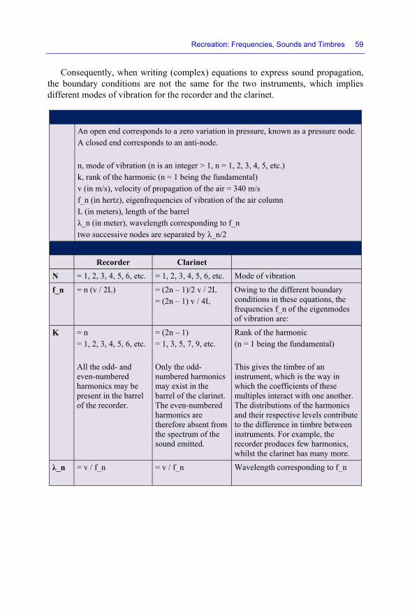
Recreation: Frequencies, Sounds and Timbres 59
Consequently, when writing (complex) equations to express sound propagation, the boundary conditions are not the same for the two instruments, which implies different modes of vibration for the recorder and the clarinet.
An open end corresponds to a zero variation in pressure, known as a pressure node. A closed end corresponds to an anti-node. n, mode of vibration (n is an integer > 1, n = 1, 2, 3, 4, 5, etc.) k, rank of the harmonic (n = 1 being the fundamental) v (in m/s), velocity of propagation of the air = 340 m/s f_n (in hertz), eigenfrequencies of vibration of the air column L (in meters), length of the barrel λ_n (in meter), wavelength corresponding to f_n two successive nodes are separated by λ_n/2
Recorder Clarinet N = 1, 2, 3, 4, 5, 6, etc. = 1, 2, 3, 4, 5, 6, etc. Mode of vibration
f_n = n (v / 2L)
= (2n – 1)/2 v / 2L = (2n – 1) v / 4L
Owing to the different boundary conditions in these equations, the frequencies f_n of the eigenmodes of vibration are:
K = n = 1, 2, 3, 4, 5, 6, etc. All the odd- and even-numbered harmonics may be present in the barrel of the recorder.
= (2n – 1) = 1, 3, 5, 7, 9, etc. Only the odd-numbered harmonics may exist in the barrel of the clarinet. The even-numbered harmonics are therefore absent from the spectrum of the sound emitted.
Rank of the harmonic (n = 1 being the fundamental) This gives the timbre of an instrument, which is the way in which the coefficients of these multiples interact with one another. The distributions of the harmonics and their respective levels contribute to the difference in timbre between instruments. For example, the recorder produces few harmonics, whilst the clarinet has many more.
λ_n = v / f_n = v / f_n Wavelength corresponding to f_n
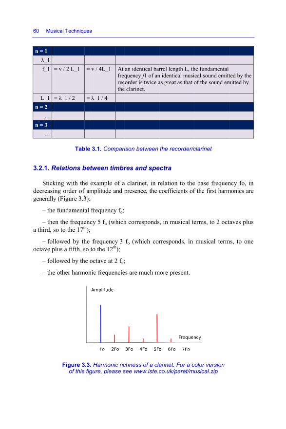
60 Mus
n = 1 λ_1 f_1 =
L_1 =n = 2
… n = 3
…
3.2.1. R
Stickdecreasingenerally
– the
– thea third, s
– folloctave p
– foll
– the
sical Techniques
= v / 2 L_1 =
= λ_1 / 2 =
Table
Relations be
king with the ng order of amy (Figure 3.3):
e fundamental
en the frequenso to the 17th);
lowed by the lus a fifth, so
lowed by the o
e other harmon
Figure 3.3of this fig
s
v / 4L_1 At freqrecthe
λ_1 / 4
e 3.1. Compari
tween timbr
example of amplitude and p:
frequency fo;
cy 5 fo (which;
frequency 3to the 12th);
octave at 2 fo;
nic frequencie
. Harmonic ricgure, please s
an identical barquency f1 of anorder is twice a clarinet.
ison between
res and spe
a clarinet, in rpresence, the c
h corresponds
fo (which cor
;
es are much m
chness of a clasee www.iste.c
rrel length L, thn identical musias great as that o
the recorder/c
ectra
relation to thecoefficients of
, in musical te
rresponds, in
more present.
arinet. For a cco.uk/paret/mu
he fundamental ical sound emittof the sound em
clarinet
e base frequenf the first harm
erms, to 2 oct
musical term
color version usical.zip
ted by the mitted by
ncy fo, in monics are
taves plus
ms, to one
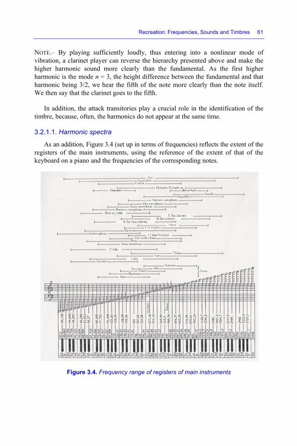
Recreation: Frequencies, Sounds and Timbres 61
NOTE.– By playing sufficiently loudly, thus entering into a nonlinear mode of vibration, a clarinet player can reverse the hierarchy presented above and make the higher harmonic sound more clearly than the fundamental. As the first higher harmonic is the mode n = 3, the height difference between the fundamental and that harmonic being 3/2, we hear the fifth of the note more clearly than the note itself. We then say that the clarinet goes to the fifth.
In addition, the attack transitories play a crucial role in the identification of the timbre, because, often, the harmonics do not appear at the same time.
3.2.1.1. Harmonic spectra
As an addition, Figure 3.4 (set up in terms of frequencies) reflects the extent of the registers of the main instruments, using the reference of the extent of that of the keyboard on a piano and the frequencies of the corresponding notes.
Figure 3.4. Frequency range of registers of main instruments
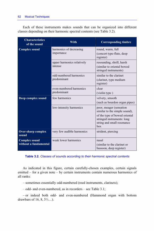
62 Musical Techniques
Each of these instruments makes sounds that can be organized into different classes depending on their harmonic spectral contents (see Table 3.2).
Characteristics of the sound
With Corresponding timbre
Complex sound harmonics of decreasing importance
round, warm, full (concert type-flute, deep register)
upper harmonics relatively intense
resounding, shrill, harsh (similar to oriental bowed stringed instruments)
odd-numbered harmonics predominant
similar to the clarinet (clarinet, type medium register)
even-numbered harmonics predominant
clear (violin type )
Deep complex sound few harmonics velvety, smooth (such as bourdon organ pipes)
low-intensity harmonics poor, meager (sensation similar to the simple sound), of the type of bowed oriental stringed instruments: long string and small resonance box
Over-sharp complex sound
very few audible harmonics strident, piercing
Complex sound without a fundamental
weak lower harmonics nasal (similar to the clarinet or bassoon, deep register)
Table 3.2. Classes of sounds according to their harmonic spectral contents
As indicated in this figure, certain carefully-chosen examples, certain signals emitted – for a given note – by certain instruments contain numerous harmonics of all ranks:
– sometimes essentially odd-numbered (reed instruments, clarinets);
– odd- and even-numbered, as in recorders – see Table 3.1;
– or indeed both odd- and even-numbered (Hammond organ with bottom drawbars of 16, 8, 5⅓…).

Recreation: Frequencies, Sounds and Timbres 63
Thus, these notes have a different timbre, due to the harmonic richness engendered by the instrument when the note is created. Certain timbres of instruments rich in “third” harmonics will already “naturally” be to the fifth and easily recognizable.
The instantaneous content and its evolution over time in the harmonic spectrum enables our auditory apparatus to recognize the instrument which produced the sound/note.
3.3. Recomposition of a signal from sine waves
In the early 19th Century, the mathematician and physicist Joseph Fourier showed that it was possible to break down any given signal into a sum of sine frequencies. Conversely, it is not too difficult to recreate these sounds (in fact, these signals and their spectral contents) using multiple sine-frequency generators. For decades now, technology has been such that numerous “instruments” known as “synthesizers” have tried (and sometimes succeeded) to reconstruct these signals, but primarily have, from all these pieces, created new sounds, thus given rise to new, entirely unknown timbres, which would have been utterly inconceivable with conventional instruments.
To briefly give a few examples of timbre recomposition, there have been two technical and technological ages: the age of subtractive synthesis followed by that of additive synthesis.
3.3.1. Subtractive synthesis
We generate a signal that is rich in even- and/or odd-numbered harmonics, or with a quasi-infinite spectrum depending on the types of simple waveforms that the signal generator can create, such as square waves, sawtooth waves, single and/or double ramp waves, white noise, pink noise, etc. Then, we try as best we can to filter the signal, using multiple electronic filters: high-pass, low-pass, pass-band, etc., to obtain the desired harmonic content by subtracting the initial spectrum.
3.3.2. Additive synthesis
We generate the desired even- and odd-numbered harmonic- and subharmonic frequencies one by one, and then add them together, weighting their respective amplitudes in order to obtain the desired harmonic content (see Figure 3.5 and a characteristic example of the harmonic drawbars of a Hammond organ in the following).
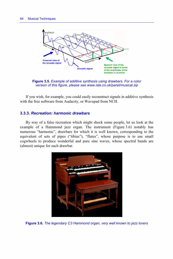
64 Mus
F
If youwith the
3.3.3. R
By wexamplenumerouequivalecogwhee(almost)
Figu
sical Techniques
Figure 3.5. Exversion of th
u wish, for exfree software
Recreation: h
way of a false of a Hamm
us “harmonic”ent of sets ofels to produceunique for ea
re 3.6. The leg
s
xample of addhis figure, plea
ample, you co from Audacit
harmonic dr
recreation whmond jazz or”, drawbars fof pipes (“tibie wonderful ach drawbar.
gendary C3 H
ditive synthesisase see www.i
ould easily recty, or Wavepa
rawbars
hich might shrgan. The in
for which it isias”), “flutes”and pure sine
Hammond orga
s using drawbiste.co.uk/pare
onstruct signaad from NCH.
hock some peonstrument (Fis well known”, whose pure waves, who
an, very well k
ars. For a coloet/musical.zip
als in additive .
ople, let us logure 3.6) not
n, correspondirpose is to uose spectral b
known to jazz l
or
synthesis
ook at the tably has ng to the
use small bands are
lovers

Each indicatedgradationof sound
– theclassified
– the
– the
Thus
Thusmiddle oappropria single octave, ichord inintended able to dproducina recorde
of the drawbad in “feet” (onns indicated o
d intensity (pu
e 16', 8', 4', 2d by octave, fr
e drawbars 5⅓
e 13/5' drawbar
s, we have laid
s, if your origof the keyboiately drawn ogo, with just
its fifth and itsnstead of a sind by the compodo this, of coung one sinusoier also produc
ars correspondne foot = 12 inon each of theut, bluntly the v
2', 1' drawbarfrom low to hi
⅓' and 2⅔' and
r corresponds
d the foundatio
Figure 3.7. Cset of drawb
inal stave sayoard, and, forout the 8', the 4t one finger, ys higher thirdngle note; thioser and writteurse, with a ridal note at a tces some harm
Recreation:
ds to a dimensnches of 2.54
e drawbars – fvolume!) the p
rs obviously cigh;
1⅓' are dedic
to a set of thir
ons (see Figur
Correspondencbars and the n
ys to play justr example, to4', the 5⅓', theyou have play– meaning th
is obviously aen on the sheerecorder, whitime (this asse
monics).
Frequencies, S
sion of equivacm = 30.5 cm
from 1 to 8 – player wishes
correspond to
cated to sets of
rds.
re 3.7).
ce between thenotes played
t one note – so create a “jae 13/5' drawbayed four noteshat in fact, youalters the entiet music… Yoch, for its paertion is actua
Sounds and Tim
alent length of m), from 1' tocorrespond to
s to assign to e
o sets of pipe
f fifths;
e
say the “C” (dazz sound”, y
ars and slightlys at once: theu have createdire harmony ou would not hart, is only caally not entirel
mbres 65
f the tibias o 16'. The o the dose each one:
es (flutes)
do) in the you have y on 1', in e note, its d a lovely originally have been apable of ly true, as

66 Mus
Oncecouplingpedal int
Obvifabulousaround y
sical Techniques
Figfrom
e again, we hg players makto the bargain
iously, with ts timbre becyour initial no
s
gure 3.8. A fewm the instructio
have not mentke between th!
that combinatause the harote is much r
w typical regisons for the C3
tioned all thee upper and l
ion, that partrmonic contericher. It may
strations extrac3 Hammond or
e notions of dlower keyboar
ticular set of ent thus creay even be tha
cted rgan
deliberate andrds, and some
drawbars, yoated (additiveat after small
d frequent etimes the
ou have a ely here) doses of

Recreation: Frequencies, Sounds and Timbres 67
each drawbar, the sound obtained, with and thanks to these harmonics, is close/ resembling another instrument – hence the names of certain specific sets of organs see figure 3.8.
EXAMPLE.– In the “reed” family of sounds, let us take the second proposed setting: the clarinet, listed as “00 60 70 540” – see Table 3.3.
In the decoded version, to give the sound of “Clarinet 8'”, we take no 16' (of course, this is too deep), nor its natural fifth (triple its frequency), 5⅓'. However, there is quite a lot of 8' (understandable, as we are emulating a Clarinet 8'), no 4' or 1' (too high – again, we are aiming for a Clarinet 8'!), a little fifth 2⅔' to create the characteristic “to the fifth” sound of the clarinet, and finally the little “smidge” of the third 13/5' and fifth 1⅓' for the final coloration on request. Thus, in an auditive and additive fashion, you have recreated the content of a Fourier spectral decomposition which is close to a certain clarinet.
Drawbars 16' 5⅓' 8' 4' 2⅔' 2' 13/5' 11/3' 1'
Volume 0 0 6 0 7 0 5 4 0
Table 3.3. Example of Hammond registration of “Clarinet 8'”

4
Intervals
The stage is set. We have chosen to employ a series (or arsenal) of notes (frequencies) which are clearly defined and carefully distributed (in our case, twelve different notes) which we have named in increasing order (for now) along the length of the reference octave:
1 2 3 4 5 6 7 8 9 10 11 12 do do# ré ré# mi fa fa # so so# la la# ti and do
We shall now take an in-depth look at the gaps/distances in frequency separating the notes from one another.
4.1. Gap/space/distance/interval between two notes
In musical language, the term “intervals” is used to speak of the gaps between two given notes (frequencies).
Let us go back, for a moment, to the example of the method of physical generation of notes in the form of multiples of frequencies, as it truly is “mindlessly” physical. The start of the scale of frequencies (notes) thus defined can be described as a succession of harmonic frequencies (“true” harmonics –multiples) as follows:
N being the value of the integer multiple in question.
Musical Techniques: Frequencies and Harmony, First Edition. Dominique Paret and Serge Sibony. © ISTE Ltd 2017. Published by ISTE Ltd and John Wiley & Sons, Inc.

70 Musical Techniques
Rank of the octave 0 1 2 3 do0 do1 so1 do2 mi2 so2 ti♭2 do3 ré3 mi3 ... f0 × N ; N = × 1 × 2 × 3 × 4 × 5 × 6 × 7 × 8 × 9 × 10 ...
Whatever the method for generating notes, depending on the value separating one note from another, we can name the intervals (see Table 4.1 for an example).
Value of the number Example Name of the interval two do to ré interval called second
three do to mi third
four do to fa fourth
five do to so fifth
six do to la sixth
seven do to ti seventh
eight do to do+ octave
nine do to ré+ ninth
... ... ...
Table 4.1. Naming of the intervals
4.2. Measuring the intervals
Obviously, to quantify intervals, however random they may be, we need to be able to measure them reliably. There are two commonly employed methods, using two different types of units: the Savart and the Cent.
4.2.1. The savart
In view of the fact that the correspondence between the notes and their respective frequencies is logarithmic, acoustic physicists can accurately quantify the interval between two notes of any given frequencies f1 and f2, using a particular unit of measurement: the “savart”. Its definition is as follows:
Interval of f2 from f1 = 1000 × [log10 of (f2/f1)] in savarts
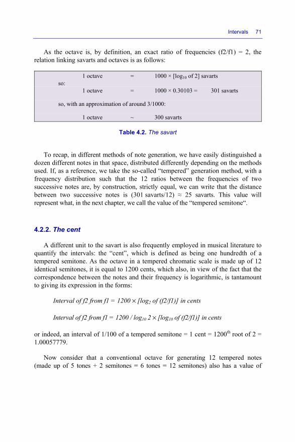
Intervals 71
As the octave is, by definition, an exact ratio of frequencies (f2/f1) = 2, the relation linking savarts and octaves is as follows:
1 octave = 1000 × [log10 of 2] savarts so: 1 octave = 1000 × 0.30103 = 301 savarts
so, with an approximation of around 3/1000:
1 octave ~ 300 savarts
Table 4.2. The savart
To recap, in different methods of note generation, we have easily distinguished a dozen different notes in that space, distributed differently depending on the methods used. If, as a reference, we take the so-called “tempered” generation method, with a frequency distribution such that the 12 ratios between the frequencies of two successive notes are, by construction, strictly equal, we can write that the distance between two successive notes is (301 savarts/12) ≈ 25 savarts. This value will represent what, in the next chapter, we call the value of the “tempered semitone“.
4.2.2. The cent
A different unit to the savart is also frequently employed in musical literature to quantify the intervals: the “cent”, which is defined as being one hundredth of a tempered semitone. As the octave in a tempered chromatic scale is made up of 12 identical semitones, it is equal to 1200 cents, which also, in view of the fact that the correspondence between the notes and their frequency is logarithmic, is tantamount to giving its expression in the forms:
Interval of f2 from f1 = 1200 × [log2 of (f2/f1)] in cents
Interval of f2 from f1 = 1200 / log10 2 × [log10 of (f2/f1)] in cents
or indeed, an interval of 1/100 of a tempered semitone = 1 cent = 1200th root of 2 = 1.00057779.
Now consider that a conventional octave for generating 12 tempered notes (made up of 5 tones + 2 semitones = 6 tones = 12 semitones) also has a value of
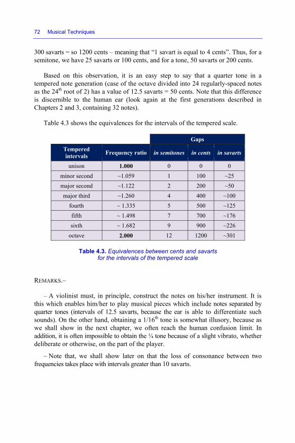
72 Musical Techniques
300 savarts = so 1200 cents – meaning that “1 savart is equal to 4 cents”. Thus, for a semitone, we have 25 savarts or 100 cents, and for a tone, 50 savarts or 200 cents.
Based on this observation, it is an easy step to say that a quarter tone in a tempered note generation (case of the octave divided into 24 regularly-spaced notes as the 24th root of 2) has a value of 12.5 savarts = 50 cents. Note that this difference is discernible to the human ear (look again at the first generations described in Chapters 2 and 3, containing 32 notes).
Table 4.3 shows the equivalences for the intervals of the tempered scale.
Gaps Tempered intervals Frequency ratio in semitones in cents in savarts
unison 1.000 0 0 0
minor second ~1.059 1 100 ~25
major second ~1.122 2 200 ~50
major third ~1.260 4 400 ~100
fourth ~ 1.335 5 500 ~125
fifth ~ 1.498 7 700 ~176
sixth ~ 1.682 9 900 ~226
octave 2.000 12 1200 ~301
Table 4.3. Equivalences between cents and savarts for the intervals of the tempered scale
REMARKS.–
– A violinist must, in principle, construct the notes on his/her instrument. It is this which enables him/her to play musical pieces which include notes separated by quarter tones (intervals of 12.5 savarts, because the ear is able to differentiate such sounds). On the other hand, obtaining a 1/16th tone is somewhat illusory, because as we shall show in the next chapter, we often reach the human confusion limit. In addition, it is often impossible to obtain the ¼ tone because of a slight vibrato, whether deliberate or otherwise, on the part of the player.
– Note that, we shall show later on that the loss of consonance between two frequencies takes place with intervals greater than 10 savarts.

Intervals 73
– Given that a semitone in tempered note generation is equal to 25 savarts, and represents a frequency ratio equal to 1.059, which is around a 6% frequency gap; a gap of 1 savart represents 1.059/25, so around 6%/25 = 0.24% frequency gap.
This is all very well, but how can we put it to use? It is perfectly simple: we now have a tool to quantify the note-to-note gaps from one method of note generation to another. To put this more simply, we can quantify the “quality” (consonance, dissonance, harshness, etc.) of the gap existing between a note created by an instrument “with mechanical harmony” – e.g. a hunting horn – and the note of the same name created on a piano, finely tuned using the tempered method. “Well, it is practically the same thing”, one might say. So what?
4.3. Intervals between notes
In the particular case of note generation by the frequency-multiple method to which our western ears are accustomed (through education, culture, etc.) and which we have adopted, once this is done, we can numerically express the distances (or ratios) between certain notes, so:
do1 do2 so2 do3 mi3 so3 ti♭3 do4 ré4 mi4 N = ×1 ×2 ×3 ×4 ×5 ×6 ×7 ×8 ×9 ×10 Name of interval Value of the frequency ratio of the interval Octave from do2 to do1 2/1 Fifth from so2 to do2 3/2 Fourth from do3 to so2 4/3 Major third from mi3 to do3 5/4 Minor third from so3 to mi3 6/5 7/6 8/7 “Major” tone – e.g. from ré4 to do4 9/8 “Minor” tone e.g. from mi4 to ré4 10/9 ………………..
Table 4.4. Distances/ratios between two notes

74 Musical Techniques
Similarly, we have the intervals presented in Table 4.5.
The value of the gap corresponding to two consecutive tones – from mi to do in the same octave, for example – is: mi4 / do4 = 5/4 so = (mi4/ré4) × (ré4/do4) = (10/9) × (9/8) = 10/8 = 5/4 The fifth corresponds to the stack of = mi3 to do3 + so3 to mi3 = major third + minor third or indeed: stacking (or “addition”) of the intervals = product of the frequency ratios = 5/4 × 6/5 = 6/4 = 3/2
Table 4.5. Examples of additions of intervals
This whole wonderful world would resonate harmonically very well together (using simple fractions of integers) and would have a strong tendency to be consonant. In addition, often, our ear would prefer the addition of the “daddy” of the music family: do1 (or its twin, do2), to make the sound rich, attractive and complete (in hertz, of course!), and, for good measure, we could even add, as required, the do4, which, within the overall consonance, would hardly be perceived at all.
The values contained in the table initially highlight the following intervals: fifth 3/2, major third 5/4, minor third 6/5, minor seventh, ninth, etc., which are, in fact, the building blocks of the notes which will (in Chapter 9) make up major chords, minor chords, M7, m7 and 9 chords, etc. The earliest notions of harmony, the first harmonic chords and the first basslines would be born!
4.3.1. Second interval: major tone and minor tone
In this mode of physical note generation, we also see the appearance of the notion of a “major tone” interval and a “minor tone” one. Indeed, the second interval from do4 to ré4 (9/8) is slightly greater (hence the name “major”) than the second from ré4 to mi4 10/9 (hence the name “minor”). Can you believe it? You are right to. Indeed, if we crudely reduce them to the same denominator, we obtain:
9/8 = 81/72, which is greater than 10/9 = 80/72
which is a gap between the two “major and minor” tones of 1/72 – i.e. a 1.38% gap. This gap between the major tone and the minor tone is known as the syntonic comma (see later on in the chapter).

Intervals 75
4.3.2. Major third and minor third interval
The thirds from do4 to mi4 (equal to that from do3 to mi3) and mi3 to so3 do not have the same value. What a scandal! The first has a value of 5/4, ((mi4/ré4) × (ré4/do4) = (10/9) × (9/8) = 10/8 = 5/4), and the second from so3 to mi3 has a value of 6/5, i.e. of the order of 25/20 and 24/20. The third from do to mi is therefore “majorly” greater than 25/24 - greater by 4.166% than the “minor” third from mi to so.
Obviously, if we had used a “tempered” mode of note generation, none of this would ever have happened!
4.4. Overview of the main intervals encountered
Table 4.6 gives the conventional names applied to the intervals that may be found with a series of 12 notes (tempered or otherwise) per octave.
# # # # # #
C D E F G A B C D E
b b b b b b
Name of interval Notation Constitution
min. second m2 ½ tone x x d
Maj. second M2 1 tone x x d
min third. m3 1 tone ½ x x c
third M3 2 tones x x c
augmented third 3+ 2 tones ½ x x
perfect fourth P4 2 tones ½ x x d
augmented fourth 4+ 3 tones x x
diminished fifth 5° 3 tones x x
perfect fifth P5 3 tones ½ x x
augmented fifth 5+ 4 tones x x
min.sixth. m6 4 tones x x
Maj. sixth M6 ; 7° 4 tones ½ x x
min. seventh m7 5 tones x x
Maj. seventh M7 5 tones ½ x x
octave P8 6 tones x x
Table 4.6. Conventional names of the intervals with a series of 12 notes per octave. The terms in italics are redundant terms
to speak of certain intervals
76 Musical Techniques
REMARKS ABOUT TABLE 4.6.–
– The augmented fourth or diminished fifth containing an interval equal to three tones is called a “triton”.
– In the table, the letters “c” and “d” indicate the consonance or dissonance of the intervals when the two notes are played simultaneously (see Chapter 5).
4.5. Quality of an interval
The quality of an interval depends not only on the “frequency distance” between the two notes making it up, but also on numerous other parameters. Let us cite the following examples.
4.5.1. Instrumentation
Every instrument (including the human voice) has its own specific characteristics of harmonic richness of its timbre, and therefore (numerous) underlying intervals between harmonics, which may also be considered notes.
4.5.2. Tempo
The tempo is the length of time for which the interval is maintained, depending on the melody of the piece being played. Having mentioned the temporal concepts of dynamics and statics earlier on, we have linked the ideas of consonance dissonance to a temporal aspect, so they are linked to the tempo of the melody.
4.5.3. Dynamics of amplitudes
The relative amplitudes of two sounds in the interval emitted at a given time can change the content of the consonance or dissonance of the interval.
4.5.4. Register
Notes of the same name do not have the same degree of importance in terms of the quality of the interval, depending on whether they are located in the same octave or in a nearby one. Thus, a dissonant interval from do3 to ré3 will sound almost consonant from do3 to ré4, representing a greater absolute gap between the two frequencies.
Intervals 77
4.6. Reversal of an interval
The reversal of an interval remains an interval – a new one, certainly different, but an interval nevertheless!
EXAMPLE.– The permutation of the two notes – do3, so3 – in the form of a reversal – to so3, do4 – changes the nature, the quality, and hence, the nature of the interval has changed! The fifth interval from do3 to so3 becomes a fourth from so3 to do4, and it does not sound the same! The same is true of the intervals cited above.
Let us now switch to the long story of commas!
4.7. Commas…ss
Before going into a detailed view of commas…ss, which will later help to understand the lengthy pages on harmony, let us state generally that comma(s) are extremely small intervals (see the numerous paragraphs below), generally between roughly a tenth (5 savarts or 20 cents) and a fifth (10 savarts or 40 cents) of a tone.
NOTE.–
– Caution: these values are not the smallest frequency difference between two sounds perceptible to an untrained human ear. Indeed, our brains are capable of discerning differences of around 1/100 of a tone in frequential/harmonic sync (sounds heard simultaneously) and sometimes even more!
– In actual fact, there is no precise definition of “a comma”. Each of the commas described below refer to and are usually measured in cents, so they can be quantified and classified.
– In the absence of further clarification, musicians generally consider that a tone (whose value is 200 cents) is, by definition, equal to 9 commas, so a comma is declared, without another form of process, has a value of 200/9 = 22.22 cents (in fact, it is a poorly defined side/approximation between the values of the Pythagorean- and syntonic commas which we shall describe below)!
– Knowing that in a generation of tempered notes, the ratio between the frequencies of two successive notes separated by a semitone is 1.05946, and the frequency gap between a la at 440 Hz and a la# = 440 × 1.05946 = 466.16 Hz is therefore 26 Hz = 100 cents, which makes the comma 22.22 cents equivalent to 5.7 Hz.
This latter interval corresponds approximately to the gap in frequency between a la at 440 Hz and another la at 446 Hz, so a 6 Hertz gap, which represents a musical accuracy of the ear of a seasoned musician of 6/440 = ~1.4%.
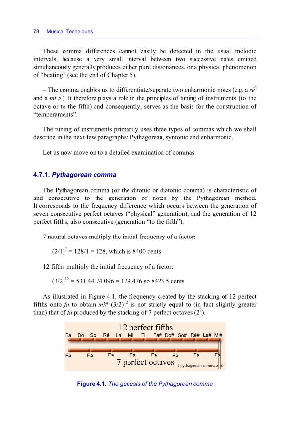
78 Mus
Thesintervalssimultaneof “beati
– Theand a mioctave o“tempera
The tdescribe
Let u
4.7.1. P
The Pand conIt correspseven coperfect f
7 nat
(2
12 fif
(3
As ilfifths onthan) tha
sical Techniques
e comma dis, because a eously generaling” (see the e
e comma enabi♭). It therefoor to the fifth)aments”.
tuning of instin the next fe
us now move o
Pythagorean
Pythagorean cnsecutive to ponds to the
onsecutive perfifths, also con
tural octaves m
2/1)7 = 128/1 =
fths multiply t
3/2)12 = 531 4
llustrated in Fnto fa to obtaat of fa produc
Figur
s
ifferences canvery small
ly produces eiend of Chapte
bles us to diffore plays a role) and consequ
truments primew paragraphs
on to a detaile
n comma
comma (or ththe genera
frequency difrfect octaves (nsecutive (gen
multiply the in
= 128, which
the initial freq
41/4 096 = 12
Figure 4.1, theain mi# (3/2)12
ced by the stac
re 4.1. The ge
nnot easily binterval betw
ither pure dissr 5).
ferentiate/sepae in the principuently, serves
marily uses thrs: Pythagorean
ed examination
he ditonic or dation of notefference whic(“physical” ge
neration “to th
nitial frequenc
is 8400 cents
quency of a fa
29.476 so 842
e frequency cr2 is not strictcking of 7 per
enesis of the P
be detected iween two sucsonances, or a
arate two enhaples of tuningas the basis f
ee types of con, syntonic and
n of commas.
diatonic commes by the h occurs betweneration), an
he fifth”).
cy of a factor:
actor:
3.5 cents
reated by the tly equal to (irfect octaves (
Pythagorean c
in the usual ccessive notesa physical phe
armonic notes of instrumen
for the constr
ommas whichd enharmonic
ma) is charactPythagorean
ween the genend the generat
stacking of 1in fact slightl27).
omma
melodic s emitted
enomenon
(e.g. a ré# nts (to the ruction of
h we shall .
teristic of method.
eration of tion of 12
12 perfect ly greater

Intervals 79
By comparing these two quantities, we can see an appreciable auditory difference (around 1/16th of a tone) and the relative ratio of the frequencies has the value of the Pythagorean comma, so:
Δfo / fo = ((3/2)12 – (2/1)7) / fo = (312– 219) / 219 = (531441– 524288) /524288 = 1.0136432 = around 23.46 cents
4.7.2. Syntonic comma
The syntonic comma, which is characteristic of the way in which Aristoxenus saw (or rather heard!), corresponds to the interval existing between four consecutive perfect fifths and two octaves augmented by a pure major third. It is also the interval between a minor tone and a major tone.
The stacking of four perfect fifths produces a Pythagorean third (starting from do → do, so, ré, la, mi) different to the natural third of a syntonic comma.
4 perfect fifths correspond to a multiplication of the frequency by (3/2)4 = 81/16.
To bring that ratio within an octave, we need to divide it by 4 → 81/64 = 1.265625.
The third do - mi obtained by the octave-based generation method is equal to 5/4 so 80/64 = 1.25.
The value of the syntonic comma is therefore:
= (81/64) / (80/64) = 1.0125 = around 21.50 cents
It is therefore slightly less than the Pythagorean comma (see above).
The Pythagorean third is higher than the natural third of 21.5 cents (the approximate value of the syntonic comma) and higher than the equally tempered third of 7.8 cents.
Thus, the natural third is less than the tempered third, by 13.7 cents.

80 Musical Techniques
4.7.3. A few remarks about commas
There are numerous other commas: maxime comma, magna comma, but the Pythagorean comma (~23.5 cents) and syntonic comma (21.5 cents) are the most important.
4.7.4. Enharmonic comma
In an instructive detour, let us cite the following points as a reminder.
4.7.4.1. (Small) sharp
The enharmonic comma, also known as a (small) sharp, is the value of the interval existing between three major thirds and an octave. It is also the interval between the chromatic semitone and the diatonic semitone of the natural scale with pure thirds. By the same calculation methods, we would have obtained a value of:
= 128/125 = 1.024 are around 41.05 cents
4.7.4.2. Large sharp
The large sharp is the value of the interval existing between four minor thirds and an octave. Its value is:
= 648/625 = 1.0368, so around 62.56 cents
4.7.5. Other theoretical commas and a few additional elements
4.7.5.1. Holdrian comma
Given that an octave has a total of 6 tones, i.e. 1200 cents, and that musicians have decided unilaterally that a tone was made up of nine commas (the diatonic, semitone, four; the chromatic semitone, five), the value of Holder’s comma divides the octave into 53 = ((6 × 9) – 1) and its value, very close to the Pythagorean comma is:
= 1200/53 (a 53rd of an octave of 1200 cents) = around 22.64 cents

Intervals 81
4.7.5.2. Sauveur comma
The Sauveur comma is approximately one 43rd of an octave, and its value is:
= 1200/43 = around 27.90 cents
4.7.5.3. Schisma
We have noted that two trains of thought led to the Pythagorean (1.0136432) and syntonic commas (1.0125), whose values are similar but slightly different. A third way is to search for a definition of a comma – the Schisma – as having a value as close as possible to 1! This was made with the difference in frequencies which takes place between the generation of 5 consecutive perfect octaves (so “physical” generation, 25) and the generation of 8 perfect fifths, also consecutive (so generation “to the fifth“, (3/2)8) augmented by a third (5/4), so numerically expressed, it is (5/22) × (3/2)8 / 25 = (5 × 38)/215.
Its value is (5 × 38)/215 so:
= 32,805/32,768 = 1.001129 so 1.95 cents, which is approximately 2 cents = 2,657,205/2,654,208 = 1.001129
Hence, this is almost the value equal to the difference between the Pythagorean and syntonic commas:
= 531,441/524,288 – 81/80 = 1.0136432 – 1.0125 = 1.001143
To define this comma, the best approximate value of the type (n + 1)/n, where n is an integer sometimes used, is 886/885 = 1.0011299.
Approximately speaking, the syntonic comma has a value of 11 schismas, and the Pythagorean comma 12.
4.7.5.4. Diaschisma
The comma or interval diaschisma is obtained by composing (descending) two perfect thirds (the factor 52) and four perfect fifths (the factor 34).
Its value is 211/(52 × 34), which is 2048/2025 = 1.011358, so around 19.55 cents.

82 Musical Techniques
These commas and the schisma are theoretical, “paper” values, and are not musical values.
Let us now move on from commas and give a few other useful comments.
4.7.5.5. The (big) tone
The Pythagorean tone is also called the large tone. In the Pythagorean scale, there is only one tone, and its ratio is 9/8. It is therefore 3.9 cents larger than the tempered tone, and its value is 203.9 cents.
4.7.5.6. The Limma
The Limma, sometimes called the Diaton-Limma, is the diatonic semitone of the Pythagorean scale (e.g. from do to ré♭). This interval is expressed by the ratio 256/ 243 = 1.05349, which makes 90.2 cents.
It is 9.8 cents smaller than the tempered semitone, which is equal to 100 cents.
4.7.5.7. The apotome
The apotome, sometimes called the Chromate-Apotome, is the chromatic semitone of the Pythagorean scale (e.g. from ré♭ to ré). Its value is naturally one tone less a Limma, which makes: ((9/8) – (256/243)), so 2187/2048 = 1.067877, which is 113.7 cents.
It is 13.7 cents greater than the tempered semitone, which is equal to 100 cents, and if we compare it to the Limma, the difference between the two is a Pythagorean comma, so (2187/2048) – (256/243) = 531,441/524,288 = 1.0136432.
4.7.6. Final remarks
In the Baroque period (from the 16th to the 18th Century), the thirds then in use in the Pythagorean scale, by principle, sounded a little wrong and thus when one chose, for example, to redistribute the Pythagorean comma over four fifths (do-so-ré-la-mi) then the third interval do-mi lost a Pythagorean comma. Cut short by a syntonic comma, this do-mi third becomes perfect (ratio 5/4) but given the quasi-equivalence between the Pythagorean and syntonic commas, this serves the purpose in calculating the “temperaments”, which, being devoted to redistributing the Pythagorean comma, in reality primarily aimed to reduce the falseness of the thirds linked to the syntonic comma.

Intervals 83
Differences in commas, although they are typically not very audible, or even inaudible in certain intervals, are, in others, sources of dissonance which is sometimes extremely pronounced (see “wolf fifth”). Thus, commas have caused problems for music theorists who have sought to distribute the comma in different ways.
Final point: take care not to confuse “temperament” with “equal temperament”.
4.7.7. In summary, commas and C°
Appellations Values of the ratios Δf / f = Values in cents
Values in savarts
Octave 2 2 1200 301 tempered semitone
21/12 1.05946 100 25
tempered tone 21/6 1.1224554 200 50 Pythagorean tone
9/8 1.125 203.9 50.975
Commas tempered 1 schisma 2657205/2654208 1.001129 1.95
diaschisma 2048/2025 1.011358 19.55 Syntonic 81/80 1.0125 21.50 5.375
“musician’s” comma
200 cents value of 9 commas
200/9 22.22 5.5
Holdrian comma
1200/53 22.64
Pythagorean comma
531441/524288 1.0136432 23.46 5.865
Sauveur comma 27.90 enharmonic
sharp 128/125 1.024 41.05
large sharp 648/625 1.0368 62.56 Other values
Limma 256/243 1.05349 90.2 Apotome 2187/2048 1.067877 113.7
Table 4.7. Overview and summary of commas and C°

84 Musical Techniques
NOTE.– All the ratios named above always refer to the quotient of the highest value of a frequency to that of a lower frequency, with the latter being the nearest harmonic following that of the lowest. Readers may feel this is pointless, but in actual fact it is very important in acoustic terms!

5
Harshness, Consonance and Dissonance
Up until now, we have presented the existing intervals which characterize two notes taken completely separately in time, without the concept of temporal evolution and focusing only on their “static” aspect.
In this short chapter, we shall examine what comes of the interpretation of two notes played “simultaneously”. What physiological impressions are given by the interpretations of the intervals? Is it harmonious? Is it dreadful?
With this in mind, we need to define new concepts.
5.1. Consonance and dissonance
Consonance and dissonance are relative concepts which subjectively define the ratio between two sounds emitted simultaneously. The goal of this chapter is to elucidate all the “technical” details regarding these notions, but for now, let us simply state that these ideas of consonance and dissonance also depend on a psychological aspect owing to our western educations, traditions, esthetic values, customs and sociocultural conditions.
5.1.1. Consonant interval
We say that an interval is consonant when it produces a pleasant sensation: relaxing, calming, of wellbeing, and of resolution.
Intervals with these peculiarities typically have common harmonic frequencies in simple ratios of values (2/1, 3/2, 4/5, etc.) which strengthen one another.
Musical Techniques: Frequencies and Harmony, First Edition. Dominique Paret and Serge Sibony. © ISTE Ltd 2017. Published by ISTE Ltd and John Wiley & Sons, Inc.

86 Musical Techniques
5.1.2. Dissonant interval
We say that an interval is dissonant when it causes the ear an unpleasant sensation – a tension, which needs to be resolved.
Short of a voluntary act, our education tends to want to resolve this tension by bringing it to rest. That said, this lends dissonance a temporal notion of duration, passage and dynamics, entirely different to consonance which, for its part, underlies a temporal, static notion of rest. It is only a short step from here to the observation that the final tuning of a piece will (tend to) be 99.9% consonant.
5.2. Harshness of intervals
Here again is a new aspect. The difference, however small it may be, between two notes, gives a more or less marked impression of the “harshness” of the interval. Interesting, is it not? Indeed, “harshness”, “dissonance”, “consonance” and “harmonic relation” are “cousins-german”, as J.S. “Bac” would say!
Table 5.1 shows the values of the relative and cumulative gaps (in savarts) for the different notes, depending on the methods of their creation (physical, fifths or tempered), and the note-to-note gaps taken from one mode of generation in relation to another indicate the harshness of those modes.
Name of interval
Physical generation Generation to the fifth* Tempered generation
Frequency ratios
Cumulative gaps
Frequency ratios
Gaps Gaps
note to note cumulative note to
note cumulative
name values savart savart savart savart Savart Do 1 0 1 - 0 - 0 Ré second 9/8 51 9/8 (m) 51 51 50 50 Mi major third 5/4 97 81/64 (m) 51 102 50 100 Fa fourth 4/3 125 4/3 (d) 23 125 25 125 So fifth 3/2 176 3/2 (m) 51 176 50 175 La sixth 5/3 222 27/16 (m) 51 227 50 225 Ti♭ 7/4 23 250 25 250 Ti seventh 243/128 (m) 51 301 25 275 Do octave 2 300 ~ 2 23 324 25 300
*(m) obtained by ascending fifths; (d) obtained by descending fifths
Table 5.1. Relative and cumulative gaps (in savarts) between notes depending on the methods of their creation (physical, fifths or tempered)

Harshness, Consonance and Dissonance 87
NOTE.– From generation to generation and from note to note, the gaps are only slight (2 to 3 savarts), but as indicated by the highlighted areas in Table 5.2, in certain cases, they become much greater (third and sixth, for example – 3 to 5 savarts).
We have all this down on paper. Now all readers need to do is to listen and test for themselves the harshness of the interval to realize the physical effects produced by these differences.
5.3. Consonance and dissonance, tension and resolution of an interval
5.3.1. Consonance of an interval
5.3.1.1. Law number 1
A sound is more consonant when the value, expressed in the form of the ratio between the harmonic and fundamental frequencies involved is written simply. Consonance gives the ear an impression, a sensation, of calm, of restfulness, of wellbeing, and of closure.
Name of interval Values of F ratios Mode of generation
octave 2
minor third 6/5 1.2000 ~ ré# ascending-fifth generation
third 5/4 1.250 mi physical generation
fourth 4/3 1.3333 fa descending-fifth generation
fifth 3/2 1.5 so physical and ascending-fifth generation
minor sixth 8/5 1.6000 ~ so# ascending-fifth generation fifth
sixth 5/3 1.6666 ~ la descending-fifth generation
7/4 ti♭
Table 5.2. Examples of consonant intervals
5.3.1.2. Law number 2
Consonance persists if the value of that ratio between the harmonic and fundamental frequencies is, not equal, but very close, to a ratio which is simple to express. The ear is able to appreciate this gap, and this new, different, subjective

88 Musical Techniques
impression is known as “harshness” (see above). It is here that our old friend the savart comes back into play, depending on the value of the gap.
Value of gap Subjective impression - less than 2 savarts imperceptible to the ear (or else effect of consonance)
- between 2 and 8 savarts always an effect of consonance, but with an increasing degree of harshness with the number of savarts
- greater than 8 and at most 10
loss of consonance (or the presence of dissonance)
Table 5.3. Consonance and harshness
Take, for example, a value of 5 savarts (which is, in fact, one tenth of a tone, as a tempered tone is equal to 50 savarts) – a value for which we always obtain an impression of consonance, but also the sensation of harshness of the interval. This means that the individual is able to detect that two or more frequencies are present simultaneously, but unable to say which two frequencies they are, as they are consonant. To say that the notes are separate and therefore dissonant, we need to increase the distance to around 8-10 savarts (i.e. around a sixth of a tone), which also means that the maximum number of notes we are able to hear in an octave would be 300/(8 to 10) = approximately 35, which harps back to the considerations of the first chapter!
Knowing that a savart is equal to (300th root of 2), so 1.00231316, meaning that a frequency ratio of 0.23% between two savarts:
Imperceptible 0.46%
Increasing harshness 0.46 to 1.84%
Loss of consonance 1.84 to 2.3%
Our 5 savarts give a coefficient of:
1.00231316 to the power of 5 = 1.01161944
10 savarts give us:
1.00231316 to the power of 10 = 1.02337389
Thus, when we play a la3 = 440 Hz (an “A” note), harshness occurs at:
440 × 1.01161944 = 445.112 Hz

Harshness, Consonance and Dissonance 89
and dissonance occurs from around:
440 × 1.02337389 = 450.284 Hz
and 25 savarts (which is a semitone):
1.00231316 to the power of 25 = 1.05946307 = 466.113 Hz
To clarify, this is indeed a la3#. Wow!
In the coming chapters, it should be interesting to look at how to quantify the structure of a major chord, such as do, mi, so, and examine the comparative harshness values of the intervals depending on whether these chords are constructed using notes from generations to fifth notes or tempered generation.
EXAMPLE.–
– the interval do, mi obtained to the ascending fifth has the value of 1.25 exactly;
– the interval do, mi obtained by the tempered method has the value of 1.259922, which we can say is almost equal to 1.26.
Thus, we have a difference between the two methods of 1.26/1.25 = 1.008, so 0.8%.
This value of 0.8% (within the range 0.46 and 1.84%) will give a feeling of harshness to that interval if, for example:
– two people play these two intervals simultaneously on two instruments – one tuned to fifths and the other tuned by the tempered method;
– or indeed, if someone is used to the do, mi interval of 1.25 s/he will find that (in comparison to his/her own auditory memory) the second interval is a little harsh.
In the chapter on chords, we shall look again at these ideas on whether or not the sound is pleasing, and harmony.
5.3.2. Dissonance of an interval
5.3.2.1. Law number 3
Anything that is not consonant is, in principle, dissonant, giving an impression/sensation of waiting, of lack of definition, unease and tension.
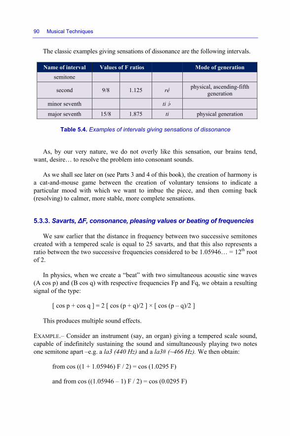
90 Musical Techniques
The classic examples giving sensations of dissonance are the following intervals.
Name of interval Values of F ratios Mode of generation semitone
second 9/8 1.125 ré physical, ascending-fifth generation
minor seventh ti♭
major seventh 15/8 1.875 ti physical generation
Table 5.4. Examples of intervals giving sensations of dissonance
As, by our very nature, we do not overly like this sensation, our brains tend, want, desire… to resolve the problem into consonant sounds.
As we shall see later on (see Parts 3 and 4 of this book), the creation of harmony is a cat-and-mouse game between the creation of voluntary tensions to indicate a particular mood with which we want to imbue the piece, and then coming back (resolving) to calmer, more stable, more complete sensations.
5.3.3. Savarts, ΔF, consonance, pleasing values or beating of frequencies
We saw earlier that the distance in frequency between two successive semitones created with a tempered scale is equal to 25 savarts, and that this also represents a ratio between the two successive frequencies considered to be 1.05946… = 12th root of 2.
In physics, when we create a “beat” with two simultaneous acoustic sine waves (A cos p) and (B cos q) with respective frequencies Fp and Fq, we obtain a resulting signal of the type:
[ cos p + cos q ] = 2 [ cos (p + q)/2 ] × [ cos (p – q)/2 ]
This produces multiple sound effects.
EXAMPLE.– Consider an instrument (say, an organ) giving a tempered scale sound, capable of indefinitely sustaining the sound and simultaneously playing two notes one semitone apart –e.g. a la3 (440 Hz) and a la3# (~466 Hz). We then obtain:
from cos ((1 + 1.05946) F / 2) = cos (1.0295 F)
and from cos ((1.05946 – 1) F / 2) = cos (0.0295 F)
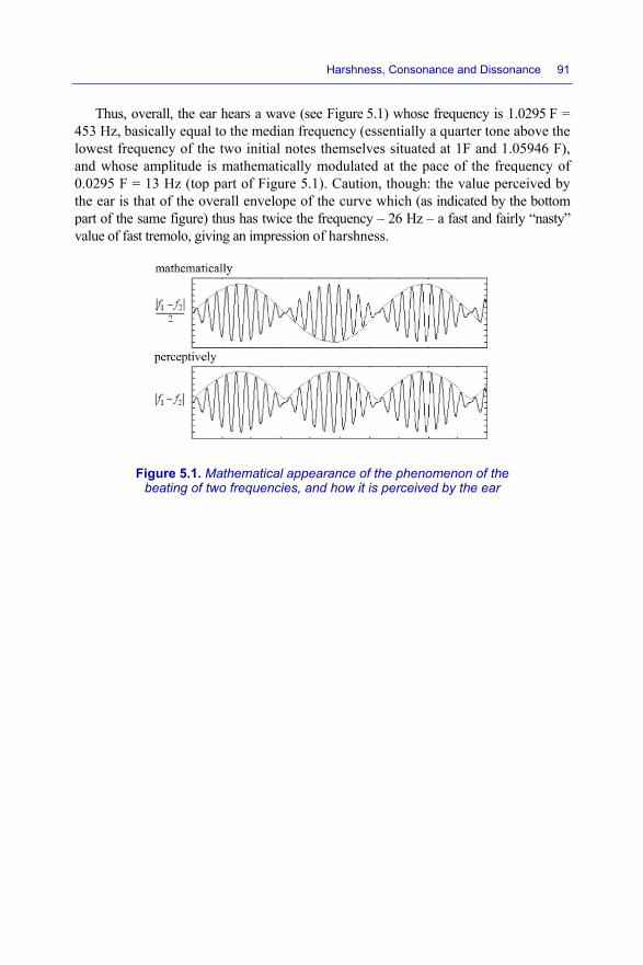
Thus453 Hz, lowest frand who0.0295 Fthe ear ipart of thvalue of f
, overall, the ebasically equa
frequency of those amplitude F = 13 Hz (tos that of the ohe same figurefast tremolo, gi
Figure 5.1. beating of
ear hears a waal to the medihe two initialis mathemati
p part of Figuoverall enveloe) thus has twiiving an impre
Mathematicaf two frequenc
Harshn
ave (see Figureian frequency notes themseically modulaure 5.1). Cautope of the curvce the frequen
ession of harsh
l appearance cies, and how i
ness, Consonan
e 5.1) whose f(essentially a
elves situated ated at the paction, though: tve which (as i
ncy – 26 Hz –hness.
of the phenomit is perceived
nce and Disson
frequency is 1quarter tone aat 1F and 1.0
ce of the freqthe value percindicated by tha fast and fairl
menon of the d by the ear
ance 91
.0295 F = above the 05946 F), quency of ceived by he bottom ly “nasty”

PART 2
Scales and Modes

Introduction to Part 2
The aim of this second part is to give greater detail about certain notions pertaining to scales and modes which we shall use, in Parts 3 and 4, to look at how to construct harmonic chords and, in particular, ultimately construct harmonious sequences. Do not complain at having to take this necessary step; rather, make the most of it to solidify the basis of your knowledge, by looking at how a great many scales came to be; their qualities; their shortcomings; what they make easier; their flexibility; and the whole bevy of awkward names we attach to them!
Without wishing to close the stable door after the horse has bolted, let us state that, in Part 1, we began by sawing little bits of wood of unequal lengths to build rungs (notes), and then classified those notes by increasing length (i.e. by their frequencies). Here, in Part 2, using these little rungs, we shall begin to construct ladders (scales), all identical in length (an octave), with unequal, irregular steps between the rungs (the intervals), and learn to climb up those ladders by stepping on not necessarily the first or second rung, or by skipping steps (modes)! This is a rough analogy, but one which quite accurately represents the discussion to be found in this part.
Now… to work!

6
Scales
6.1. Introduction to the construction of scales
Having, in the previous chapters, detailed, at length, the different methods of creation and scales of notes (generally we choose to work with a dozen notes, the values of their eigenfrequencies, etc.), followed by the concepts of intervals between the notes with the notions of semitones and tones, let us now look at the creation and organization of scales of notes, which will also be a long story!
As a short preamble to this long chapter, to clarify, summarize and simplify a complex issue that often arises with regard to two frequently-employed terms, let us state that:
– the noun “scale” (in whatever context) is the generic term defining the way in which an octave (i.e. from fo to 2 × fo), whatever the value of fo, (from ré#3 to ré#4, for example), is divided into a succession of notes (5, 6, 7, 9, 12, 24, etc.), and the distribution of those notes within that octave;
– musical “modes”, which we shall see in the next chapter, are, for their part, possible variations/paradigms from a given scale.
To define these scales, we shall speak of the gaps (tone or semitone) separating the different notes (or degrees – also see the next chapter) which make up the scales.
A scale is constructed in the way we want to link notes spaced an octave apart. We may choose two steps, six steps or fourteen steps, distributed in any which way, and we will have defined a scale. Obviously, these scales will sound different, will often be incompatible and will not be at all pleasing to the ear! Once again, there is something for everyone.
Musical Techniques: Frequencies and Harmony, First Edition. Dominique Paret and Serge Sibony. © ISTE Ltd 2017. Published by ISTE Ltd and John Wiley & Sons, Inc.
98 Musical Techniques
It is said that the Greeks (Pythagoras, Archimedes, etc.) were amongst the first to note the similarities in perception that existed between certain intervals, primarily the ratio of 2 between the heights (the octave), and then sought to divide that main and essential interval into smaller intervals to form what would later become known as scales.
On this point, sticking with considerations that are only valid in the context of “western” music, numerous approaches are possible (three in particular: principal, physical or natural, Pythagorean and tempered), depending on whether our approach draws more on physics or simply on hearing or mathematics.
6.2. Natural or physical scale
The so-called “natural” scale is based on pure multiples of frequencies known as first “harmonics” and generally includes 7 notes, though it may extend up to 12. It draws inspiration from the physical generation of notes presented in the previous chapters. By its principle, it is harmonically just, as all the notes are strictly harmonics of the same fundamental frequency – a property which lends the scale great consonance, but which, melodically, turns out to sound somewhat wrong, as the fifth-to-fifth intervals of the notes created in the “natural” scale are slightly off.
Thus, the major scale based on a do contains:
– the fifth (3/2) of do, which is so;
– the major third (5/4) of do, which is mi;
– etc.
On the subject of harmonics, let us briefly look again at the general physics of the phenomenon, and at acoustic physics in particular.
6.2.1. Harmonics
In acoustics, a harmonic is a component of a wave (sound, for our purposes) whose frequency is a multiple of the fundamental. In music, a harmonic is also called a particular partial, and is an independent component of a musical sound.
For instance, if ƒ0 is the fundamental frequency, the harmonics will have frequencies equal to: 2ƒ0, 3ƒ0, 4ƒ0, 5ƒ0, etc. (see Figure 6.1 for an example).

Scales 99
Figure 6.1. Harmonics of a vibrating string. For a color version of this figure, please see www.iste.co.uk/paret/musical.zip
If, as a fundamental note, we take “la3” (440 Hz), then harmonics are all notes whose frequency is a multiple of 440. The harmonics of a note, therefore, are necessarily higher than that note, and are known as upper harmonics.
Example Values in Hertz Hz Frequency Harmonic of rank
ƒ0 440 fundamental 1
2 × ƒ0 880 (440 × 2) first multiple 2
3 × ƒ0 1320 (440 × 3) second multiple 3
4 × ƒ0 1760 (440 × 4) third multiple 4
Table 6.1. Examples of harmonics of 440 Hz
When we speak of fundamental frequency, we speak of the frequency of the first harmonic content of the sound in question, which is labeled “harmonic 1” or fundamental (harmonic). Normally, the note we hear corresponds to the frequency

100 Musical Techniques
value of that first harmonic, even if the frequency itself is absent from the sound spectrum, because sometimes, certain sounds can mislead the ear – a harmonic of a higher rank can sometimes be heard more clearly than the fundamental, and mask it (see Chapter 3 on timbres).
6.3. Pythagorean or physiological diatonic. scale
At the root of the diatonic scale, there is the legend whereby Pythagoras, in a blacksmith’s forge, first discovered and established the four fundamental consonances in the musical scale: unison (ratio 1/1), octave (2/1), fifth (3/2) and fourth (4/3), and the non-consonant second major (8/9), hearing the anvil ring when hit by hammers of different weights… At least, this is how the story goes. Let us now look at how these different ratios we combined with one another to obtain a complete scale of seven notes as we know it today (do, ré, mi, fa, so, la, ti). In reality, it seems that this scale has been extrapolated from Pythagoras’ work. To verify this, of course, we would need to unearth the stone-scribed messages and e-mails of the time!
The principle behind the creation of the frequencies of notes in Pythagorean scales is based on a different principle to that of the natural scale which, starting with the first harmonic (fundamental), generates notes little by little by a succession of fifth intervals [3/2]k. As partly detailed in the previous chapter, then, this is a case of the stacking of natural fifths. They sound “correct” melodically, but are not, in fact, harmonically perfect (more specifically, the harmonic frequencies of these notes do not correspond to the multiples of the fundamental frequency, and therefore chords sound a little wrong).
6.3.1. Principle
Let us take a detailed look at the subtle aspects of this generation of notes and scales, taking up the thread of the story:
– we arbitrarily choose a starting degree – the fundamental – which we take as a unit and a reference frequency;
– we multiply the value of this frequency by 3 (in fact to exactly obtain the harmonic 3) and we obtain the value of its first natural fifth (doubled). Obviously, the fact of multiplying by 3 takes the note out of our interval [1;2] of an

Scales 101
octave. We then “normalize” the frequency of the note thus obtained by dividing it by 2 to bring it back into the interval [1;2], which gives the ratio 3/2 = 1.5, known as a “fifth”;
– having noticed that the initial note and its fifth “sounded” good together, we once again look for the value of the frequency of the fifth of the last note found by multiplying it, in its turn, by 3/2. Its frequency is 3/2*3/2 = (3/2)2 = 9/4 which, expressed in the interval [1;2], gives us 9/8 = 1.125. For example, consider an initial la3 = 440 Hz. The natural fifth mi is equal to 440 × (3/2) = 660 Hz, and the fifth of that fifth, the ti (the ninth), is equal to 440 × (3/2) × (3/2) = 440 × (3/2)2 = 990 Hz;
– and so on. We apply that fifth interval, little by little, to our reference note whose frequency is 1: we then “normalize” the note obtained by dividing it by 2 as many times as is necessary to bring it back into our octave [1;2].
IMPORTANT REMARK.– At the 5th note thus obtained, fairly regularly spaced, we could stop. Some theorists have indeed stopped there, and we would have obtained the 5-note major pentatonic scale which is used in jazz in its tempered form – particularly in “blues” music (see later on in this chapter).
The fifth next frequency is (3/2)5 = 243/32, which gives us 243/128. We now have the possibility for a 6-note (hexatonic) scale.
6.3.2. The why and wherefore of the 7-note scale
We go up one more notch, and that is where the trouble starts!
Horror of horrors, the frequency value of that 7th note expressed in the interval [1;2] is 1.0679, rather than 1, as is much to be hoped to bring it back to the octave (see Table 6.2)! It was known from the start that with this method of generating notes in a geometric progression of [3/2]k, we could never reach an integer multiple of 2, the octave.
On principle, this series ([3/2]k geometric progression) gives an infinite creation of notes, the first 25 of which are given as an example in Table 6.2.
The right-hand column shows the normalized values of these notes expressed in the reference octave, and all these notes “sound good together”, because they respect the gap of the natural fifth. However, there are an infinite number of notes, which is far too many! Therefore, we need to restrict ourselves.

102 Musical Techniques
k (3/2)k n 2n (3/2)k/2n 0 1.0000 0 1 1.0000 1 1.5000 0 1 1.5000 = 3/2 2 2.2500 1 2 1.1250 = 9/8 3 3.3750 1 2 1.6875 = 27/16 4 5.0625 2 4 1.2656 = 81/64 5 7.5937 2 4 1.8984 =
243/128 6 11.391 3 8 1.4238 7 17.086 4 16 1.0679 8 25.629 4 16 1.6018 9 38.443 5 32 1.2014 10 57.665 5 32 1.8020 11 86.498 6 64 1.3515 12 129.75 7 128 1.0136 13 194.62 7 128 1.5205 14 291.93 8 256 1.1403 15 437.89 8 256 1.7105 16 656.84 9 512 1.2829 17 985.26 9 512 1.9243 18 1477.9 10 1024 1.4433 19 2216.8 11 2048 1.0824 20 3325.3 11 2048 1.6237 21 4987.9 12 4096 1.2177 22 7481.8 12 4096 1.8266 23 11,223 13 8192 1.3700 24 16,834 14 16,384 1.0275 25 25,251 14 16,384 1.5412 etc.
Table 6.2. Generation of notes in [3/2]k geometric progression. For a color version of this table, please see www.iste.co.uk/paret/musical.zip
Considering that the reported value of the 7th fraction obtained (highlighted in red) is already very close to 1 (= 1.0679), it seemed at that stage that we had found the first integer multiple – i.e. 2× – of the fundamental; simply put, that the error was correct! Thinking that we had almost closed the loop – and remaining conscious of what is not completely true – we stopped at 7 notes to form the diatonic Pythagorean scale!

Scales 103
Thus, curiously, to define and close the loop of the Pythagorean scale, the 7th note chosen is not that which would be defined and calculated by the next fifth, but the value rounded to exactly 2, based on the fact that 2 (the octave) is in harmony with the fifth, but it is also in harmony with note whose fifth it is, and whose frequency is 2/3, because 1 = 3/2*2/3, which gives us 4/3 in the interval [1;2] (see Figure 6.2).
The Pythagorean scale is, in fact, a fine “juggling act” between generation of notes to the fifth (and therefore melodic) and recovery to the octave by physical generation of notes (thus harmonic)!
In addition, Figure 6.2 shows the successive order of occurrence of the notes as a function of the values of the harmonics involved from 1 to 27, and the boxed area illustrates the previous section.
Natural 1 2 3 4 5 6 7 8 9 10 11 12 13 14 16 17 18 19 20 21 22 23 24 25 26 27 Pythagorean 1 3 9 27 Pythagorean + octave 1 2 3 4 8 9 16 27 Pythagorean + octaves 1 2 3 4 6 8 9 12 16 18 24 27 ….
Figure 6.2. Order of appearance of the notes as a function of the values of the harmonics involved from 1 to 27. For a color version
of this figure, please see www.iste.co.uk/paret/musical.zip
A few further remarks:
– reading Table 6.2, we ought to have gone up to the 12th value (area highlighted in blue), which represents a diatonic scale with 12 notes, to come a little closer to the octave, (1.36% gap), instead of 6.7% with 7 notes… We would also have needed six fingers per hand (a fair few, then!) to play and cover all the holes in a 12-hole flute;
– the fourth note in the scale may fly in the face of what we are used to (we may consider that it needs to be lower). This stems from the fact that it has not been preserved exactly (the theoretical value was 729/512), but replaced with 3/4, which has a very close value.
Note that this frequency of 3/4 is none other than the fourth which we saw earlier. It would have been a shame not to include it in this scale. If we, in turn, find the fifth of that fourth, we of course obtain the higher octave (3/4 × 3/2 = 2). This is logical, as we saw earlier that the fourth was the complementary interval of the fifth.

104 Musical Techniques
6.3.3. Names of the notes in the Pythagorean scale
We have now defined (found) the 7 notes in the Pythagorean major scale, but how are we to name them? It is well known that it was around the 11th Century that they were named and linked to the degrees which we know today: that was when the monk Guido of Arezzo had the idea of using the first syllables of the Gregorian chant Hymn to Saint John the Baptist, written in Latin verse by the poet Paul Diacre:
Ut queant laxis
Resonare fibris
Mira gestorum
Famuli tuorum
Solve polluti
Labii reatum
Sancte Iohannes
In the 18th Century, the syllable Ut was replaced by the “do” for Domine. In the author’s native France and Latin countries, this naming system has been widely adopted, as opposed to the alphabetic notation C, D, E, F, G, A, B which is always used in Germanic or English-speaking countries. Also, in the 19th Century, Sarah Glover changed the “Si” to “Ti” (“a drink with jam and bread”, in the popular memory aid), so that each musical syllable would begin with a different letter: D, R, M, F, S, L, T… D.
Figure 6.3, below, recaps the notes of the well-known (almost Pythagorean) scale, with the exact values of the frequencies in the form of fractions, generation to the fifth, their little arrangements and the names of the notes as we know them, and a higher do exactly at double the frequency of the lower do… By principle, this situation cannot exist in a fifth-based model of note generation!
Figure 6.3. Final notes of the famous scale (almost Pythagorean)

6.3.4. T
Let uthe diffe
Alonbetween
– eith
– or a
Betwbetween the lengt1 semitoimpressi
Pythagoscale
T
In adthan thespecifica
to
The series “t
us look again rent frequency
Figure 6.4
ng the whole othe notes (Fig
her an interval
an interval wi
Figure 6.5. T
ween certain nothers, ratios
th of the scaleone - 1 tone -ion of hearing
do
orean e
1
Table 6.3. Seq
ddition, in this e succession ally, the freque
one/(2 semiton
tone-tone-se
at the Pythagy ratios which
4. Frequency r
of this scale, gure 6.4):
l with a value
th a value of 2
Tone- and sem
notes, we haves of 256/243 e we have form- 1 tone - 1 a “normal” sc
# #
ré 1
quence of tone
scale, we can(cascade) of
ency ratio is:
nes) = 1.125/1
emi/tone-ton
gorean scale (h are present b
ratios present
we observe t
of 9/8 = 1.12
256/243 = 1.0
mitone interval
e ratios of 9/8(known as Py
med, gives thetone - 1 semcale (Figure 6
mi fa ½ 1
es and semiton
n see that the tf two semito
1.10985 = 1.0
ne-tone-ton
(shown in Figbetween succe
in the Pythago
that there are
5, defining a t
0534979, defin
ls in the Pytha
(known as Pyythagorean see order sequen
mitone. Thus, 6.5).
# #
so 1
nes in the Pyt
tone of 9/8 = 1ones (256/243
136
Sca
e-semi/tone
gure 6.4) and essive notes.
orean scale
two types of
tone;
ning a semiton
agorean scale
ythagorean tomitones) whi
nce of: 1 tone we (may) re
#
la t1 ½
thagorean sca
1.125 is slight3)2 = 1.1098
ales 105
e”?
calculate
f intervals
ne.
ones), and ch, along - 1 tone - ceive the
ti do ½
ale
tly greater 85. More

106 Mu
This certainlywe shall recap, twapproximChapters
6.3.5. A
1) Wdifferent octave [Pythagordreadful;identicalprinciple
2) Th
Fo
3) Wdoes notThere is
usical Technique
difference, my perceptible trevisit later wh
welve perfect mation there is 3 and 4 on in
A few comme
With the originto the do, but
[1;2], the easyrean comma. ; it is what il transpositione, impossible.
he succession
igure 6.6. Sucobtained from
Wolf fifth: we t produce a coa slight extra
es
measuring aroto the human hen we compafifths are appris none other ntervals).
ents
nal Pythagoret because we ay solution chThe fifth mi#
is known as ns and modula
of ascending
ccession of asWikipedia). Fo
www.iste
showed earliomplete loop
a interval. The
ound 1/9 of aear. It is know
are the Pythagoroximately eqthan the Pyt
ean scale [3/2are ultimately ohosen consists#/ti# (or fa/dothe “wolf fi
ations (preserv
fifths is illustr
scending fifthsor a color vers.co.uk/paret/m
ier that the mto achieve th
erefore, there w
a tone, is nown as the Pythorean scale toqual to seven pthagorean com
2]k, by princiobligated to fis of shortenin
in the enharfth” (see nexving the same
rated in Figur
s (illustration usion of this figumusical.zip
method based he exact octavwill inevitably
ot insignificanhagorean comm the temperedperfect octavemma – look
iple, the ti# ist the scale into
ng the last firmonic systemxt section). Te melodic scal
re 6.6.
under GNU FDure, please se
on the seriesve of the fundy be a fifth tha
nt, and is ma, which d scale (to es, and the
again at
s slightly o an exact ifth by a
m) sounds Therefore, le) are, in
DL, ee
s of fifths damental. at is badly

Scales 107
placed! This interval (which thus sounds rather wrong) has been dubbed the wolf fifth, because it seems to “howl” (like a wolf) when we use it… For precisely this reason, though, it does not tend to be used!
4) All instruments tuned to the fifth or the fourth are predisposed to this usage. Numerous examples have been presented, showing that it is impossible (or at least extremely difficult) for a violinist to play in a system other than the Pythagorean, due to the simple fact that the instrument is, by its constitution, tuned to perfect fifths. Typically, of the very numerous ways to tune a violin, its four open strings are tuned to so, ré, la and mi, and violas, cellos and double basses are respectively tuned to descending fifths below this pattern.
5) Polyphony (as the name suggests: the act of playing several notes at once) is constructed by progressively sounding degrees further and further away from the fundamental, from the most consonant to the most dissonant. Thus, to begin with, we have the octave; then the fifth (or the fourth, which is a consequence of the fifth); the third; the seventh; the ninth, etc. In the Pythagorean scale, the fifths are perfect. Nonetheless, these so-called perfect fifths are ill suited for playing chords of three simultaneous 3, as the Pythagorean major third is very high, at 81/64 = 1.2656, and sounds bad in relation to the value of the physical perfect third, which is at 5/4 = 1.125, which produces a difference of 81/80 (i.e. 21.5 cents – see previous chapter) which seems unacceptable to the ear. The tendency to voice the “perfect chord“ including both the third and the fifth has led to the evolution of the passage, moving away from a scale with very strained harmonies (with its dissonant thirds) toward a much softer harmony, with natural thirds.
6.3.6. Uses of the Pythagorean scale, and cases where it cannot be used
Although it is archaic, dating from over 3000 years ago, the Pythagorean scale is still in use today, including in the western world, and has a marked impact on our perceptions and on harmony.
Just a few remarks.
6.3.6.1. In Greece
The musical system employed by the Ancient Greeks is extremely complex. The Pythagorean scale is purely theoretical, and as no man is a prophet in his own land, the Greeks did not use that scale wholesale in their own musical practices. In fact, the scales used are extrapolated from Aristoxenus’ scale.

108 Musical Techniques
6.3.6.2. In China
In China, the idea of a scale had already existed for several centuries before Pythagoras, and was viewed as symbolic and magical in origin. The ordering of the scale is identical to the Pythagorean scale, and it too is constructed by calculation. This scale is organized in relation to the origin degree and the reference to the tonic is significant. The first four steps in this scale sound like an anhemitonic pentatonic system (that is to say, one which contains no semitones – for instance, starting at do, the scale would go do ré mi so la). Additionally, these are the only degrees actually used by the Chinese; the pentatonic scale is generated from any one of the five degrees. In China, this model is theoretical and practical, and it is still in use for traditional music.
These remarks and this recurrence represents a veritable archetype in music, omnipresent in almost all musical traditions the world over, and shows that the vast majority of scales are generated in the same way.
6.4. Major diatonic scale
The so-called “major” scale use a particular set of seven notes out of the 12 created earlier (in fact, a particular distribution of frequencies in the reference octave).
For example, if we take, as a base note – or reference note, or indeed “tonic” note – the note known as “do”, and select the seven notes already mentioned frequently – “do, ré, mi, fa, so, la and ti”, in the octave, we define what it is helpful to call the major scale “ of do” or indeed the “do major scale”:
–reference octave:
…la ti do ré mi fa so la ti do ré…
– or the English version:
A B C D E F G A B C D
The do, called the “tonic”, represents the tone in which the piece is played, so we have the “C major“ or “C maj” scale.
6.4.1. Intervals present in a major scale
Let us now examine the different intervals present in this particular range of the octave from do to do, and which constitute the organization/architecture of any so-called “major” scale – see Table 6.4.

Scales 109
Total scale = 6 tones
Do 1 } 1 tone } tetrachord = 2½ tones
Ré 2 } 1 tone
Mi 3 } ½ tone
Fa 4 } 1 tone separation of tetrachords interval from 4 to 7 = tritone (3 tones) So 5 } 1 tone } tetrachord = 2½ tones
La 6 } 1tone
Ti 7 } ½ tone
Do 8
Table 6.4. Positioning of tetrachords in a major scale
6.5. The other major scales
Using the same architecture of tones and semitones, we can construct any major scale in any key.
A classic construction is to work with close tonalities, which are, as it happens, harmonics (3rd-order), forcing those which are a fifth above or a fifth below.
The specific quality of this well-known construct, called the “circle of fifths”, progressively displays, in turn:
– either all the sharps in ascending-fifth generation;
– or all the flats in descending-fifth generation.
6.6. Scales and chromatic scales
In structural terms, the 7-note diatonic scale has a slight limitation: it is impossible to transpose! Indeed, if we simply transpose this scale by, say, increasing each note by a semitone, those notes would not all fall (even approximately) onto existing notes in the original scale. The mi would be transposed to the fa, and the ti to the do, but the rest would fall “between two notes”. The solution to this problem is to add a note into each whole-tone interval (there are five of them), to divide/split it into two semitones. This then enables us to combine, mix and alternate natural tones and semitones, and this new scale then uses steps of a semitone (or, if we so desire, a quarter tone, etc.) and gives different colors to the soundscape – hence the name “chromatic”. This is the proposal of the chromatic scale which we shall envisage, and is made up of 7 + 5 = 12 notes.

110 Mu
6.6.1. C
The cdegrees notes obof the fidenticala semitothe adjacblur”.
As pare equadependinclassic esemitonediatonic tnotes).
6.6.2. C
There
usical Technique
Chromatic sc
classic chromain the diatonictained by altefive tones in l). The scale, tone, apart of ecent intervals
reviously indial in size), theng on the alteraexample of aes in the Pythtones and semi
Fo
Chromatic sc
e are two chro
es
cale
atic scale is a c (do, ré, mi, f
erations (# andthe diatonic
then, is now mequivalent sizoften blurs th
icated (excepte chromatic a
ation used (by sa diagram givhagorean scaleitones; the inte
Figure 6.7. Apof the semiton
cales
omatic scales:
musical scalefa, so, la and
d♭) of the origc scale into tmade up of twzes (or almosthe frames of r
t for the tempand diatonic ssharpening or fving an appre (the chain b
ermediary notes
pproximation ones in the Pyth
one ascendin
e composed onti), and five a
ginal notes, whtwo semitone
welve degrees t equivalent). reference, tend
pered scale, wsemitones areflattening a notoximation of
brackets indicas in parenthes
of the placemehagorean scal
ng, and the oth
n the basis of additional intehich divide (ae (but not ne(12 semitonesThis quasi-id
ding to lead to
where all the se not at the sate). Figure 6.7
f the placemenate the positioes are so-calle
ent le
her descending
the seven ermediary alter) each ecessarily s), spaced dentity of o a “tonal
semitones ame place, 7 shows a nt of the
ons of the ed altered
g.

Scales 111
6.6.2.1. Ascending chromatic scale
To construct the ascending chromatic scale, we continue with our mathematical series of the Pythagorean scale, and we can see that the next time we “almost close the loop” (i.e. almost get back to a frequency whose value is 1), when the exponent k = 12. The frequency of the note, then, is 1.0136 (see Table 6.2).
The five additional notes obtained will be notes altered to the #, and the set of the 12 notes gives a chromatic scale, called ascending because it is based on ascending fifths. It should be noted that the fraction 729/512 eliminated a little earlier in the diatonic scale reappears, becoming the fa#.
6.6.2.2. Descending chromatic scale
In just the same way as we calculated our ascending scale on the basis of ascen-ding fifths, we could apply the same principles with descending fifths, i.e. by looking for the preceding fifths, little by little, instead of taking the next fifths.
To do this, we need to divide (instead of multiplying) by 3/2, which is equivalent to multiplying by 2/3. The series will be as follows: 2/3; 4/9; 8/27; 16/81, up to 4096/531,441 on the 12th iteration. This series must then be normalized to bring all the values back in to the interval [1;2].
Thus, we obtain a different chromatic scale known as descending, because it is based on descending fifths. The notes thus formed correspond to the flats.
6.6.2.3. 25-note chromatic scale
Figure 6.8 gives a view of the conclusions of the previous sections with ascending and descending chromatic scales.
In the case of an octave from do to do, the rules placed underneath the clef indicate the distribution of the semitones in the ascending and descending chromatic scales
Figure 6.8. Ascending and descending chromatic scales
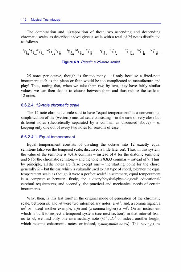
112 Musical Techniques
The combination and juxtaposition of these two ascending and descending chromatic scales as described above gives a scale with a total of 25 notes distributed as follows.
Figure 6.9. Result: a 25-note scale!
25 notes per octave, though, is far too many – if only because a fixed-note instrument such as the piano or flute would be too complicated to manufacture and play! Thus, noting that, when we take them two by two, they have fairly similar values, we can then decide to choose between them and thus reduce the scale to 12 notes.
6.6.2.4. 12-note chromatic scale
The 12-note chromatic scale said to have “equal temperament” is a conventional simplification of the (western) musical scale consisting – in the case of very close but different notes (theoretically separated by a comma, as discussed above) – of keeping only one out of every two notes for reasons of ease.
6.6.2.4.1. Equal temperament
Equal temperament consists of dividing the octave into 12 exactly equal semitone (also see the tempered scale, discussed a little later on). Thus, in this system, the value of the semitone is 4.416 commas – instead of 4 for the diatonic semitone, and 5 for the chromatic semitone – and the tone is 8.833 commas – instead of 9. Thus, by principle, all the notes are false except one – the starting point for the chord, generally la – but the ear, which is culturally used to that type of chord, tolerates the equal temperament scale as though it were a perfect scale! In summary, equal temperament is a compromise between, firstly, the auditory/physical/physiological/ educational/ cerebral requirements, and secondly, the practical and mechanical needs of certain instruments.
Why, then, is this last true? In the original mode of generation of the chromatic scale, between do and ré were two intermediary notes: a ré♭, and, a comma higher, a do# or indeed another example, a fa and (a comma higher) a mi#. On an instrument which is built to respect a tempered system (see next section), in that interval from do to ré, we find only one intermediary note (ré♭, do# or indeed another height, which become enharmonic notes, or indeed, synonymous notes). This saving (one

Scales 113
note out of two) allows the development of instrumental technique and virtuosity, particularly in regard to instruments with a keyboard or keys – saxophones, clarinets, etc. The advantage of equal temperament is that, not content with saving one out of every two notes on the instrument in question, it also enables us to play all the possible alterations – as far as double sharps and double flats – without having to modify the instrument’s tuning. With this system, it becomes possible to modulate or transpose a melody into any of the twelve tonalities in the chromatic scale.
The usual choice of alterations of the 12-note Pythagorean scale, also called the natural scale, and used from Antiquity to the 16th Century, is as follows:
do; do#; ré; mi♭; mi; fa; fa#; so; so#; la; ti♭; ti
Unfortunately, though, as indicated earlier (see Figure 6.10), in this chromatic scale with 12 notes, we can see that there are two semitone values: the first 256/243 = 1.05349 and the second 2187/2048 = 1.06787!
Figure 6.10. Pythagorean scale with 12 notes and corresponding gaps
A few small additions
1) The musical instruments affected by temperament are:
– fixed-sound instruments, also known as tempered instruments:
- examples: keyboard instruments (piano, organ, harpsichord, harmonium, accordion, celesta, etc.); certain stringed instruments (guitar, mandolin, lute, harp, viol, etc.); wind instruments with keys or pistons (trumpet, tuba, clarinet, oboe, etc.);
– the other instruments are called natural instruments:
- examples: voice, certain fretless stringed instruments played with a bow (violin, viola, cello, etc.), certain wind instruments (Breton bagpipes, bombard, slide trombone, etc.).
2) When tempered instruments play with natural instruments, it is very often the temperament system which wins the day: by instinct, the violinist will tune his/her instrument to the piano, and therefore will play in tempered mode. However, from the standpoint of the notation of sheet music, we continue to respect the

114 Musical Techniques
representation of a note, and take care not to confuse the nomenclature of the enharmonic notes. For example, do# and ré♭ may well have the same height on a fixed-sound instrument, but it is important to carefully differentiate them, because they do not have the same function.
3) From the theoretical point of view, as we saw in the previous chapter, it is the Pythagorean system of note generation, divided into 53 Holdrian commas, which must be used as the “reference scale”, because it at once justifies both the theory of alterations and the creation of tonalities.
To do this, we remove the altered notes near to the natural notes, and keep only one alteration in each tone interval
4) Wolf fifth. In the 12-note Pythagorean-based chromatic scale, it is the fifth so#/mi♭ which proved false, due to the relatively arbitrary simplifications when going from 25 to 12 notes. Other choices could have rendered that fifth just, but this would simply have shifted the problem, because then another fifth would have been wrong.
6.7. Tempered scale
Dating from the 17th Century, the so-called tempered scale strikes a delicate balance between the above two systems of scale generation, with all the remarks made above, and enables us to treat the sharps and flats equally, obtained in the two ways mentioned above.
6.7.1. Principle of the tempered scale
In the tempered scale, the 12 intervals (like the first two) between the notes obtained and used become regular and equal to 21/12 (via their logarithms) and can be used to easily play in any tonality/key (transposition).
6.7.1.1. Intervals in the tempered scale
In relation to the tonic of do, the intervals thus become:
do #/♭ ré #/♭ mi fa #/♭ so #/♭ la #/♭ ti do
Scale Appellation
Tempered 1 21/12 22/12 23/12 24/12 25/12 26/12 27/12 28/12 29/12 210//12 211/12 2 Tempered
Table 6.5. Intervals in relation to the tonic
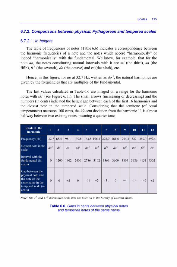
Scales 115
6.7.2. Comparisons between physical, Pythagorean and tempered scales
6.7.2.1. In heights
The table of frequencies of notes (Table 6.6) indicates a correspondence between the harmonic frequencies of a note and the notes which accord “harmoniously” or indeed “harmonically” with the fundamental. We know, for example, that for the note do, the notes constituting natural intervals with it are mi (the third), so (the fifth), ti♭ (the seventh), do (the octave) and ré (the ninth), etc.
Hence, in this figure, for do at 32.7 Hz, written as do-1, the natural harmonics are given by the frequencies that are multiples of the fundamental.
The last values calculated in Table 6.6 are imaged on a range for the harmonic notes with do1 (see Figure 6.11). The small arrows (increasing or decreasing) and the numbers (in cents) indicated the height gap between each of the first 16 harmonics and the closest note in the tempered scale. Considering that the semitone (of equal temperament) measures 100 cents, the 49-cent deviation from the harmonic 11 is almost halfway between two existing notes, meaning a quarter tone.
Rank of the harmonic 1 2 3 4 5 6 7 8 9 10 11 12
Frequency (Hz) 32.7 65.4 98.1 130.8 163.5 196.2 228.9 261.6 294.3 327 359.7 392.4
Nearest note in the scale do-1 do1 so1 do2 mi2 so2 tib2 do3 ré3 mi3 fa#3 so3
Interval with the fundamental (in cents)
0 1200 1902 2400 2786 3102 3369 3600 3804 3986 4151 4302
Gap between the physical note and the note of the same name in the tempered scale (in cents)
0 0 +2 0 – 14 +2 – 31 0 +4 -14 – 49 +2
Note: The 7th and 11th harmonics came into use later on in the history of western music.
Table 6.6. Gaps in cents between physical notes and tempered notes of the same name

116 Musical Techniques
Figure 6.11. Image of the values in Table 6.6 across a range
The gaps of the harmonics with the notes in the tempered scaleare specific to the rank of the harmonic and are found no matter what the fundamental note.
6.7.2.2. In intervals
Table 6.7 indicates the intervals (ratio between two heights, two degrees) in relation to the tonic do in the case of the three main scales: physical, Pythagorean and tempered.
do ré mi fa so la ti do
Scale Appellation Natural 1 9/8 5/4 21/16 3/2 13/8 15/8 2 Harmonic
Pythagorean 1 9/8 81/64 4/3 3/2 27/16 243/128 2 Melodic
Tempered 1 2 2/12 2 4/12 2 5/12 2 7/12 2 9/12 2 11/12 2 Tempered
Table 6.7. Intervals in relation to the tonic in the three main scales: physical, Pythagorean and tempered
NOTE.– Note that in principle, a piano tuned to the tempered scale and a wind instrument (on which certain high notes are physically/mechanically produced only as harmonics of lower notes) can never be totally tuned. In fact, the possibility of modifying the height of the notes on those two instruments – playing firstly on the fingering or the airflow for the wind instrument, and secondly on the duration and intensity of the sound for the piano – and the ear’s tolerance mean that this harmonic/melodic disagreement remains more theoretical than a practical reality.
In addition, unlike generally accepted ideas, very often, a modern piano is not strictly tuned to the tempered scale. Its tuning is generally achieved by striking a delicate compromise between the different scales mentioned above. In addition, in the extremes of the register, the octaves are “stretched” in relation to the “physically just” octaves of ratio 2, to compensate for the bias of our auditory apparatus.

Scales 117
6.8. Other scales
There are many other scales, because we can construct an infinite number of other types of scales, as there are so many possible combinations. For example, we could cite:
– “western” scales made up of 12 semitones, spaced more or less logarithmically – those of Aristoxenus, Zarlin, Mercator-Holder or Delezenne, etc.;
– pentatonic scales (containing 5 notes), which are the bases for Far Eastern music (Chinese as well with 7 equal intervals), but which are also found in Celtic music or the music of Native Americans;
– scales based on linear, non-logarithmic scales (but this is fairly exceptional) in the music of Peruvian Indians;
– Arab and Indian music is built with intervals of around ¼ of a tone but which are not completely equal;
– modern jazz, scales where more exotic scales (blues, bebop, fourth chords) are constantly used; however, the diversity of the types of chords available, if only with the major (or minor) scale explains why harmonic rules are limited to these scales; scales having a natural origin (the series of fifths), therefore, are relatively well suited to carry harmony.
Let us begin the long litany of other scales!
6.9. Pentatonic scale
The word “pentatonic” comes from the Greek penta, meaning five, and tonic, which means note. Thus, the pentatonic scale is a scale when contains five notes/sounds spaced either a tone or 1½ tones apart.
NOTE.– The name “pentatonic scale” is often considered a misuse of language due to a poor translation from German, der Ton, which means both tone and sound. Penta-ton therefore means five tones or five sounds. The exact translation would be pentaphonic, corresponding to a scale of five sounds, rather than pentatonic, which implies a scale of five tones.
6.9.1. A little history, which will prove important later on
Many ancient civilizations divided the octave into five equal intervals (here we are again: first-fifth intervals – see Figure 6.12), giving five degrees, or else divided the octave into six intervals, giving six degrees, only five of which would have been

118 Musical Techniques
used. Hence, the “pentatonic” scale could not precisely be superimposed on a scale taking five sounds in our western scale, whether using the unequal temperament of the “ancients” or the equal temperament used nowadays. Certain notes are almost a quarter tone away from the corresponding ones in the sister scale.
Figure 6.12. Example of a pentatonic scale
Under the influence of the Spaniards, South American instrument manufacturers had adopted a sort of “ill-fitting system”, which enabled them to play their traditional music “a little wrongly” and, at the same time, to play melodies written in the western scale.
6.9.2. Theory
A pentatonic system is a musical scale made up of five different heights of sound. Generally, the word is used in a more restricted sense, to speak of a certain type of scale, known as the anhemitonic pentatonic, which contains no semitonic intervals (from the Greek (an-), meaning none, and (hemi-), half, to denote the semitone) – for example, a scale formed of the notes produced only by the black keys on the piano – see Figure 6.13, the framework for which is given in Table 6.8.
Figure 6.13. Another example of a pentatonic scale
# # # # # #
mi fa so la ti do ré mi fa so 1 1 1.5 1 1.5
Table 6.8. Arrangement of tones and semitones

Scales 119
A great many musical styles the world over have used or do use this type of pentatonic scale:
– blues and its derivatives (such as rock n’ roll);
– certain forms of Berber and Hungarian music;
– oriental music, including Chinese, Vietnamese and Japanese;
– Ethiopian, Javanese, Nubian, Tibetan and Mongolian music.
6.9.2.1. Pycnons (quarter-steps)
Let us take the example of a pentatonic scale starting at so (so - la - ti - ré - mi – see Figure 6.14).
Figure 6.14. Example of pycnons
The so-la-ti part of the scale is of particular importance:
– it is separated from the rest, on both sides, by the largest interval in the scale (mi-so = ti-ré = 1½ tones);
– it is the only series of intervals which appears only once (whereas ré-mi-so = la-ti-ré; mi-so-la = ti-ré-mi, etc.). Thus, for a listener, it is the main point of reference within that scale.
A Romanian ethno-musicologist, Constantin Brăiloiu, proposed calling this so-la-ti section of the scale a pycnon (from the Greek, pucnos, meaning tight; strong).
Thus, it is with the pycnon that we begin the numbering of the degrees of this scale, as indicated in the figure. This means that we can describe a melody by says that it is in mode 1, 2, etc., which essentially means that its lowest note is 1, 2, etc.
6.9.2.2. Pyens
Similarly, in that same pentatonic scale, the intervals separating the pycnon from the rest (mi-so and ti-ré) sometimes include “secondary and fluctuating” sounds, which are nevertheless inherent to the system. Brăiloiu calls these sounds pyens (etymology drawn from Chinese musical theory – we travel the world and the seven seas in the quest for musical knowledge!).

120 Mu
Pyen
– the
– the
– the
In ac
6.9.3. R
As in5 notes cexpressescale is s
6.9.3.1.
The scale of t
6.9.3.1.
The mfollows:
C
We t
– maj
- fu
- se
- th
- fi
- si
usical Technique
ns are seconda
ey may appear
eir height fluct
ey fall on the o
ctual fact, they
Reality
ndicated abovcreated in a c
ed in a singlesaid to be maj
Major penta
major pentatothe same tona
1. Example 1
major pentato
C Major = do,
ake notes 1, 2
ajor pentatonic
undamental -
econd - third
hird - fifth
ifth - sixth
ixth - octave
es
Figure 6
ary because:
r or disappear
tuates: do - do
offbeat more o
y usually appe
ve, pentatoniccircle of five octave) (the or or minor de
atonic scale.
onic scale is cality/key.
1: major pen
onic scale of d
ré, mi, fa, so,
2, 3, 5 and 6 in
c scale = do, r
second
6.15. Example
from one vers
o♯ for one, an
often than on t
ear as transient
c scales are gsuccessive fioriginal one,
epending on t
composed of
ntatonic scale
do is compose
la, ti
n the scale of C
ré, mi, so, la:
= 1 tone
= 1 tone
= 1½ tones
= 1 tone
= 1½ tones
of a pyen
sion of the me
nd fa - fa♯ fo
the beat;
t notes or appo
generally consfifths from an, etc. As per the first third i
notes 1, 2, 3,
e of do
ed of five not
C Major, whic
(do-ré)
(ré-mi)
(mi-so)
(so-la)
(la-do)
elody to anoth
or the other;
oggiaturas.
structed fromn initial note,
usual, the pit contains.
, 5 and 6 of t
tes, and const
ch gives us:
her;
m the first and then
pentatonic
the major
tructed as

Scales 121
Figure 6.16. Major pentatonic scale of do
Thus, this scale includes the following intervals, counted from the tonic note: second - major third - fifth - major sixth. By way of example (see Table 6.9), here is a representation of the intervals that make up the “major pentatonic” scale of do.
do penta major
# # # # # #
do ré mi fa so la ti do 1 1 1.5 1 1.5
Table 6.9. Intervals in the major pentatonic scale of do
We call this the “major pentatonic” scale because:
– pentatonic because the fa and the ti are lacking from our example, to obtain the pentatonic scale of do;
– major because the first third that the scale contains is major (in our example, the mi, the third note in the scale), meaning there is an interval of 2 tones between the tonic (do) and the third (mi).
Thus, the two scales – the conventional major and the major pentatonic – are extremely closely linked. If you are improvising over a piece in a major key, you can be sure that it is the major pentatonic scale that you hear in the background.
6.9.3.1.2. Example 2: major pentatonic scale of la
For reference, below are the intervals which make up the major pentatonic scale of la (the scale widely used by rock guitarists par excellence). “Rock” much more frequently uses this scale than the major pentatonic scale of do. We shall see later on that simply by adding a single note to it, we are able to create bluesy sounds.
la penta major
# # # # # # #
so la ti do ré mi fa so la 1 1 1.5 1 1.5
Table 6.10. Intervals in the major pentatonic scale of la

122 Musical Techniques
6.9.3.2. Minor pentatonic scale
The minor pentatonic scale is also composed of 5 notes, and runs tonic - minor third - fourth - fifth - minor seventh.
6.9.3.2.1. Example 1: minor pentatonic scale of do
The minor pentatonic scale of do is composed of 5 notes, and it is constructed as follows:
C minor = do, ré, mi♭, fa, so, la, ti♭
We take the notes 1, 3♭, 4, 5, 7♭ from the C minor, scale, which gives:
– minor pentatonic scale– = do, mi♭, fa, so, ti♭:
- fundamental - minor third = 1½ tones (do-mi♭)
- minor third- - fourth = 1 tone (mi♭-fa)
- fourth - fifth = 1 tone (fa-so)
- fifth - minor seventh = 1 tone and demi (so-ti♭)
- minor seventh - octave = 1 tone (ti♭-do)
This is a minor scale because the first third that it contains is a minor third (minor third = 3 semitones = 1½ tones). It is, indeed, constructed differently: it does not use the same intervals.
As an example, see below for the minor pentatonic scale of do.
do min. penta.
#/♭ #/♭ #/♭ #/♭ #/♭ #/♭
do ré mi fa so la ti do 1.5 1 1 1.5 1
Table 6.11. Intervals in the minor pentatonic scale of do
6.9.3.2.2. Example 2: minor pentatonic scale of la
There are numerous variants of the major and minor pentatonic scales. However, the pure minor pentatonic is more widely used than the rest. It is very frequently employed in most music – particularly in rock and blues. Guitarists often speak simply of “the pentatonic scale”, meaning the minor pentatonic.

Scales 123
It is worth noting that the minor pentatonic scales of Mi (E) and La (A) are particularly easy to play on a guitar, as many of the notes they contain can be played on the open strings (i.e. with no fingers pressing down), tuned to mi (E), la (A), ré (D), so (G), ti (B) and mi (e). The movable shapes/patterns which guitarists employ when playing a melody line or forming so-called “barre” chords are based on these two scales.
The la minor pentatonic scale includes the following notes and intervals.
La penta min
#/♭ #/♭ #/♭ #/♭ #/♭ #/♭ #/♭ so la ti do ré mi fa so la ti 1.5 1 1 1.5 1
Table 6.12. Intervals in the minor pentatonic scale of la
6.9.4. Relations between major and minor pentatonic scales
Let us briefly run a comparison and examine the ways in which the major pentatonic scale of do and the minor pentatonic of la correspond.
1) The major pentatonic scale of do is made up of 5 notes: do, ré, mi, so, la.
The minor pentatonic scale of la is also composed of 5 notes: la, do, ré, mi, so.
Thus, we see that the notes la, do, ré, mi, so in the pentatonic major of do are exactly the same as those in the minor pentatonic scale of la.
2) In addition, if we compare the scale of intervals in the major pentatonic with that of the minor pentatonic (Table 6.13), we see that the intervals in the minor pentatonic scale are the same as those in the major pentatonic scale, but with a small shift.
la penta minor
#/♭ #/♭ #/♭ #/♭ #/♭ #/♭ la ti do ré mi fa so la ti do
1.5 1 1 1.5 1 do penta major
#/♭ #/♭ #/♭ #/♭ #/♭ #/♭ la ti do ré mi fa so la ti do 1 1 1.5 1 1.5
Table 6.13. Comparison of the intervals in the minor la and major do pentatonic scales
Conclusion: the major pentatonic scale = the minor pentatonic scale, situated 1½ tones higher!

124 Mu
There
– the
– for detail in construcpentatonmodes st
Theswe geneincorrectbe “pentapentaton
The make upthat thesother.
Besidpentatonmode wh
6.9.5. P
Thusrather thshown in
usical Technique
e are two othe
e major pentato
those alreadythe next chap
cted from its senic scale of dotemming from
e two scales, erally refer wt use of languaatonic”. Thus,
nic scale of mi
5 notes in thap the so majore scales begin
des the majornic scale also ghich, though it
Figure
Pentatonic s
s, we understahan a simple n Figure 6.18.
F
es
er ways in wh
onic scale is c
y familiar withpter), mode II econd note, d
o. We can alsom do (C) major
which are, bywhen we speaage. Indeed, athere are many
i minor.
at scale are mr pentatonic: sn with differen
r and minor pgives rise to twt does contain
e 6.17. Examp
cale and sy
and that the tscale. This
Figure 6.18. P
ich to express
composed of th
h the concept oof the minor
do) has the samo say that the lr pentatonic.
y far, the mostak of “the peany scale mady other possibi
mi, so, la, ti ao, la, ti, ré annt notes – a m
pentatonics, wwo other modn a minor third
ples of modes
ystem
term “pentatois the differe
Pentatonic sca
s the same idea
he same notes
of mode (whipentatonic sc
me “ladder” ofla (A) minor p
t commonly usentatonic scalede up of five nilities. Let us ta
and ré. These nd mi. The onlmi in the case o
which are its bdes, which havd, has no fifths
of pentatonic
onic” refers esence between
ale and system
a:
s as its relative
ch will be expcale of la (i.e. f intervals as tpentatonic is o
sed, are thosee”. This, in fanotes would bake a final exa
are the samely notable diffof one, and a s
best-known fove no thirds, ans (see Figure 6
c scales
ssentially to athe two dist
m
e minor;
plained in the scale
the major one of the
to which fact, is an be said to ample: the
e notes as ference is so for the
forms, the nd a final 6.17).
a system, tributions
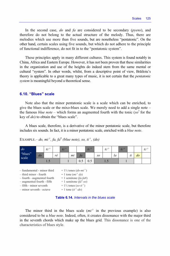
Scales 125
In the second case, do and fa are considered to be secondary (pyens), and therefore do not belong to the actual structure of the melody. Thus, there are melodies which use more than five sounds, but are nonetheless “pentatonic”. On the other hand, certain scales using five sounds, but which do not adhere to the principle of functional indifference, do not fit in to the “pentatonic system”.
These principles apply in many different cultures. This system is found notably in China, Africa and Eastern Europe. However, it has not been proven that these similarities in the organization and use of the heights do indeed stem from the same mental or cultural “system”. In other words, whilst, from a descriptive point of view, Brăiloiu’s theory is applicable to a great many types of music, it is not certain that the pentatonic system is meaningful beyond a theoretical sense.
6.10. “Blues” scale
Note also that the minor pentatonic scale is a scale which can be enriched, to give the blues scale or the mixo-blues scale. We merely need to add a single note – the famous blue note – which forms an augmented fourth with the tonic (so♭ for the key of do) to obtain the “blues scale”.
A blues scale, therefore, is a derivative of the minor pentatonic scale, but therefore includes six sounds. In fact, it is a minor pentatonic scale, enriched with a blue note.
EXAMPLE.– do, mi♭, fa, fa# (blue note), so, ti♭, (do)
do “blues” scale
#/♭ #/♭ #/♭ #/♭ #/♭ #/♭
do ré mi fa so la ti do 1.5 1 0.5 0.5 1.5 1
– fundamental - minor third = 1½ tones (do-mi♭) – third minor - fourth = 1 tone (mi♭-fa) – fourth - augmented fourth = 1 semitone (fa-fa#) – augmented fourth - fifth = 1 semitone (fa#-so) – fifth - minor seventh = 1½ tones (so-ti♭) – minor seventh - octave = 1 tone (ti♭-do)
Table 6.14. Intervals in the blues scale
The minor third in the blues scale (mi♭ in the previous example) is also considered to be a blue note. Indeed, often, it creates dissonance with the major third in the seventh chords which make up the blues grid. This dissonance is one of the characteristics of blues style.

126 Musical Techniques
6.11. Altered scale and jazz scale
In its most widely accepted sense, the term “altered scale” denotes a scale in which certain notes have been subjected to alterations, which is the case for the “jazz scale” – a scale including alterations whose role is to accentuate (by certain dissonances) the phenomenon of “tension” which is the diatonic function of the fifth-degree, chord known as the “dominant fifth”.
Let us look at an example. The notes in the “natural” minor scale in C (do) are: C D E♭ F G A B♭. However, jazz more usually uses the “ascending melodic minor scale” (or jazz minor scale), also in C: C D E♭ F G A B, which is closer to the major scale. Thus, this scale too includes seven notes (it is a heptatonic scale). We shall show in the next chapter that the altered scale is built on the seventh mode of the ascending melodic minor scale. In reference to the relevant mode of the 7th degree of the major scale, called the “Locrian” mode, the altered scale is sometimes denoted by the expression “super Locrian” mode, and in jazz, it is commonly called the “melodic minor” scale.
EXAMPLE.– The ascending melodic minor scale of do = do, ré, mi♭, fa, so, la, ti.
The 7th mode of the ascending melodic minor scale of do therefore is the altered scale of ti:
– thus, we have the altered scale of ti = ti, do, ré, mi♭, fa, so, la;
– or else, transposed into do, we have do, ré♭, ré#, mi, fa#, so#, ti♭;
where the altered notes (which do not belong to the referential key) are: ré♭, ré#, mi, fa# and ti♭.
These (altered notes or) alterations are respectively denoted by the interval which separates each of them from the fundamental of the dominant chord:
– tonic;
– minor ninth (b9);
– augmented ninth (#9);
– major third;
– augmented fourth (#4);
– augmented fifth (#5 or 5+) or minor thirteenth (b13), the double of ti;
– minor seventh.
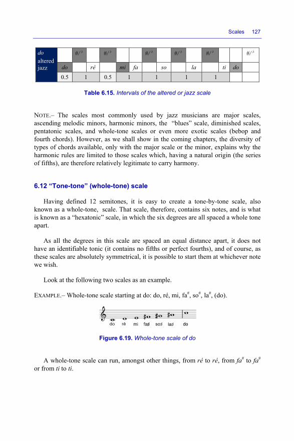
Scales 127
do altered jazz
#/♭ #/♭ #/♭ #/♭ #/♭ #/♭
do ré mi fa so la ti do 0.5 1 0.5 1 1 1 1
Table 6.15. Intervals of the altered or jazz scale
NOTE.– The scales most commonly used by jazz musicians are major scales, ascending melodic minors, harmonic minors, the “blues” scale, diminished scales, pentatonic scales, and whole-tone scales or even more exotic scales (bebop and fourth chords). However, as we shall show in the coming chapters, the diversity of types of chords available, only with the major scale or the minor, explains why the harmonic rules are limited to those scales which, having a natural origin (the series of fifths), are therefore relatively legitimate to carry harmony.
6.12 “Tone-tone” (whole-tone) scale
Having defined 12 semitones, it is easy to create a tone-by-tone scale, also known as a whole-tone, scale. That scale, therefore, contains six notes, and is what is known as a “hexatonic” scale, in which the six degrees are all spaced a whole tone apart.
As all the degrees in this scale are spaced an equal distance apart, it does not have an identifiable tonic (it contains no fifths or perfect fourths), and of course, as these scales are absolutely symmetrical, it is possible to start them at whichever note we wish.
Look at the following two scales as an example.
EXAMPLE.– Whole-tone scale starting at do: do, ré, mi, fa#, so#, la#, (do).
Figure 6.19. Whole-tone scale of do
A whole-tone scale can run, amongst other things, from ré to ré, from fa# to fa# or from ti to ti.

128 Musical Techniques
EXAMPLE.– Whole-tone scale starting at ti: ti, ré♭, mi♭, fa, so, la, (ti).
Figure 6.20. Whole-tone scale of ti
6.13. Diminished scale or “semitone/tone” scale
The diminished scale is made up of a succession of semitones and tones, which meaning that it total, it is composed of 8 notes, and by its principle, it is totally symmetrical.
In this scenario, there can only be three different diminished scales. Indeed, continuing the progression of the first three examples below, we shall see that example 4 is an exact replica (shifted by a minor third) of example 1.
– Example 1: do, ré♭, mi♭, mi, fa#, so, la, ti♭, (do)
– Example 2: do#, ré, mi, fa, so, la♭, ti♭, ti, (do#)
– Example 3: ré, mi♭, fa, fa#, so#, la, ti, do, (ré)
– Example 4: mi♭, mi, fa#, so, la, ti♭, do, ré♭, (mi♭) = Example 1
6.14. In summary
It is interesting and highly advisable to train oneself, at length, to play these different types of scales, to embed the melody lines of the scales in question into one’s ear (one’s memory, one’s brain of course).
We have taken the time to detail all these things during this chapter, because the fundaments of harmony presented in Parts 3 and 4 are based on the concepts of major, minor, tension, rest, third, fifth, seventh, etc.
Below is a table recapping the different scales mentioned and presented in this chapter, which gives a visually striking view of the different structures of the scales and the positions of the intervals (tone/semitones) relative to each of them. It is these differences which create the different “humors” expressed by harmony.

Scales 129
6.15. Technical problems of scales
There are scales and then there are scales! Consequently, choosing the right one presents a problem.
1 tone 1 tone ½tone
1 tone 1 tone 1 tone ½ tone
#/♭ #/♭ #/♭ #/♭ #/♭ do ré mi fa so la ti do
Name of scale
Number of notes
major 7
ascending melodic minor
7
harmonic
minor 7
diminished
or “semitone,
tone”
8
whole-tone 6
major pentatonic
5
minor
pentatonic 5
“blues” 6
altered “jazz”
7
etc.
Each horizontal space = ½ tone
Table 6.16. Summary and comparison of the intervals for the various scales

130 Musical Techniques
6.15.1. Scale and transposition
Depending on the type of method chosen for generating the notes (natural or Pythagorean), then, with the same names of notes, there will be scales which are slightly different because the distributions of the frequencies of the notes in the octave will be different. This means that depending on the scales obtained, the gaps between tones and semitones will be different (see Table 6.17).
Below are the values of the frequency ratios in relation to the fundamental frequency of the do in the main scales we have mentioned.
Scale do ré mi fa so la ti do
Natural 1 9/8 5/4 21/16 3/2 13/8 15/8 2
Pythagorean 1 9/8 81/64 4/3 3/2 27/16 243/128 ~2 or = 2
Tempered 1 2 2/12 2 4/12 2 5/12 2 7/12 2 9/12 2 11/12 2
Table 6.17. Gaps between tones and semitones depending on the scales
This poses an important problem: the problem of “transposition”! “What is that?” we hear you cry.
A series of musical sounds, constituting a melody, gives the ear the impression of an “air”.
However, it is possible, by modifying the frequencies of the initial notes in the melody, to create a new series of frequencies given the ear the impression of hearing the same melody, the same air. If this is done, then we say we have successfully transposed the melody (the tone).
This practice of transposition is very useful in terms of, say, accompaniments and “modulation” techniques which we shall see later on.
To return to the concrete, the necessary and sufficient condition to correctly transpose a melody is to replace the initial series of notes making up that melody

Scales 131
with another series of notes whose frequencies are apparently “translated” frequentially (logarithmically), meaning that the new frequencies are proportional to the initial frequencies.
Basic melody: note 1 2 3 4 5 6 ... Frequencies of notes F1 F2 F3 F4 F5 F6 ... Transposed melody: note 1 2 3 4 5 6 ... Frequencies of notes nF1 nF2 nF3 nF4 nF5 nF6 .... whatever the value of the factor “n”.
Figure 6.21. Principle of transposition
Taking a random value for the factor “n” is a little simplistic. The ultimate goal is to choose a value of “n” such that one of the new values “nFx” is equal to one of the frequency values belonging to the original scale. Unfortunately, it is here that things can go wrong, depending on the mode of generation used for the initial scale.
Indeed, let us look again, for a moment, at certain scales which we have already discussed.
The important problem which arises is that of the “melodic content of the melody” when transposing into other tones, depending on the modes of creation of the scales. In order for the melody to be preserved after translation, all the intervals too must be maintained after “translation”, throughout the melody, but this would only be possible if the intervals are regularly distributed within the original scale (and therefore also in the new scale), and consequently, it would be difficult or impossible with certain scales and certain instruments which generate their scales in a particular way, so the easiest way to transpose is with a scale and tempered intervals!
In conclusion, not all types of scales can be correctly transposed, and only the tempered scale allows the transposition of a melody with no problem, by the very principle of its generation.

132 Musical Techniques
Notes in the scale
do ré mi fa so la ti do
Tempered scale Interval in relation to the tonic
1 22/12
= 1.059 … … 211/12 2
Successive intervals in savarts
50 50 25 50 50 50 25
Tone = 50 savarts constant semitone = 25 savarts
Ascending-fifth scale
Interval in relation to the tonic
1 9/8 81/64 4/3 3/2 27/16 243/128 2
Successive intervals in savarts
51 51 23 51 51 51 23
Tone = 51 savarts
Inconstant semitone sometimes 51/2 = 25.5 savarts or sometimes = 23 savarts
(Physiological) or physical scale
Interval in relation to the tonic
1 9/8 5/4 4/3 3/2 5/3 15/8 2
Successive intervals in savarts
51 46 28 51 46 51 28
Major tone = 51 savarts
minor tone = 46 savarts semitone = 28 savarts
Table 6.18. Comparison between scales
6.15.2. Alterations
Here is one more technical point that must be made! Alterations – the sharp, the double sharp, the flat, the double flat, and the natural – are symbols which modify the pitch of the notes to which they are assigned.

Scales 133
Number of alterations on the clef
Major key
Natural minor key
descending fifth to fifth
0 flats C A
1 flat F D
2 flats B♭ G
3 flats E♭ C
4 flats A♭ F
5 flats E♭ B♭
6 flats G♭ E♭
7 flats C♭ A♭
ascending fifth to fifth
0 sharps C A
1 sharp G E
2 sharps D B
3 sharps A F#
4 sharps E C#
5 sharps B G#
6 sharps F# D#
7 sharps C# A#
Table 6.19. Summary of the keys as a function of the alterations present on the clef
These alterations are of different types depending on the way in which the scales are created, by generations to the ascending fifth (sharps) or the descending fifth (flats).
Table 6.19 is a classic overview of the keys in which we find ourselves depending on the number of alterations indicated on the clef.

7
Scales, Degrees and Modes
7.1. Scales and degrees
Once again, let us begin this chapter by presenting some vocabulary.
Within an octave, in creating and naming notes (look again at the previous chapters), without explicitly setting out to do so, we have created what are known as “scales” of notes whose “degrees” (bars) are distributed at intervals – regular or otherwise. Of course, in principle, these scales are repeated from one octave to another. It is for this reason that generally, a scale is represented not in linear form, but in the form of a circle, to show that it has neither a beginning nor an end, and that every point on the scale, called a degree, is a potential starting point.
For example, by a specific choice, when the octave is divided into 12 equal parts, then the circle can contain either.
Having a number of degrees Name of scales Number of different possible scales 2 Ditonics 6 3 Tritonics 19 4 Tetratonics 43 5 Pentatonics 66 6 Hexatonics 80 7 Heptatonics 66 8 Octatonics 43 9 Nonatonics 19 10 Decatonics 6 11 Undecatonic 1 12 chromatic 1
Table 7.1. Names of the scales
Musical Techniques: Frequencies and Harmony, First Edition. Dominique Paret and Serge Sibony. © ISTE Ltd 2017. Published by ISTE Ltd and John Wiley & Sons, Inc.

136 Musical Techniques
7.2. Degree of a note in the scale
Frequently, in order to facilitate scale-to-scale comparisons of the construction and to easily be able to conduct finer-grained harmonic analyses, we attribute each note an Arabic numeral representing its situation, and a Roman numeral to its “degree” in the scale in relation to the reference note in the reference scale.
It is necessary to know the degrees of a scale to understand why certain chords are labeled as “2nd”, “5th” or “1st degree” chords.
For example, in the case of heptatonic scales (containing 7 notes), the degrees in the scales of do, ti♭ and ré major are respectively indicated in Table 7.2.
Examples: scales of
Degrees Notations of degrees
Function/role Abbreviation do
major ti♭
majorré
major
1st degree I tonic T do ti♭ ré
2th degree II ré do mi
3th degree III mi ré fa#
4th degree IV sub-dominant SD fa mi♭ so
5th degree V dominant D so fa la
6th degree VI la so ti
7th degree VII sensible S ti la do#
Table 7.2. Degree of a note in a scale
7.3. Interesting functions/roles of a few degrees of the scale
In this scale (heptatonic, known as the “major” scale of “do”), with a special construction, each degree plays a role, a particular sonic function which depends on its place in relation to the first, and has a very specific name. The intuitive musical appellations of these four functions underlie the existing interdependence between those degrees, more specifically between the first (tonic), the fourth (sub-dominant) and the fifth (dominant). Indeed, between these three degrees (“functions”), there are direct physical relations (look again at the earlier chapters) because in the case that we are now dealing with (“major” heptatonic):
– the fifth degree (dominant) represents an interval of the “upper fifth” of the first degree (tonic), so an initial frequency relation of the ratio (3) × (1/2) = 3/2;

Scales, Degrees and Modes 137
– the fourth degree (sub-dominant) represents an interval of an octave of the “lower fifth” of the first degree (tonic), so an initial frequency function of the ratio 2 × (1/3) = 2/3.
In other words, once again, whilst tending to resolve on its lower fifth, all of these wonderful tonics, dominants and sub-dominants tend to resolve one another mutually:
upper so → do dominant → tonic
do → lower fa tonic → sub-dominant
Moral: the tonic is torn between its dominant and its sub-dominant, and therefore, the key of do major is not totally affirmed by this duality of resolution to the fifths. As we shall see later on:
– as so tends to resolve to do... are we operating in do major?
– as do tends to resolve to fa... are we operating in fa major?
Up to this point, nothing could be less certain. It is here that the idea of what is perceptible to the human ear comes into play to differentiate the ex æquo and set the tone.
7.4. Modes
As stated at the very start of the previous chapter, the musical “modes” presented in this chapter are possible variations or paradigms of a given scale. As we saw, there are many different kinds of scales (majors, minors, pentatonics, tone-tone, etc.), and there will be just as many different modes!
Unlike scales, which were represented in the form of circle, modes are represented on a straight line, because there is a clearly defined starting point on the scale, and thus, the scale engenders its own modes by the choice of a principal degree as the starting point.
NOTE.– The scale can also be represented directly in note form without choosing a mode, but in that case, there will be no hierarchy between its notes.
A mode has multiple peculiarities:
– in relation to a primary degree, the mode can be defined a particular series of intervals (e.g. a tone and ½ a tone, or for instance, a tone and ¾ of a tone). For example, with a 12-degree chromatic scale, with each degree corresponding to a

138 Musical Techniques
semitone, so a total of 6 tones per octave, we could have either a mode which everyone knows well: T, T, ½T, T, T, T, ½T = 6T, or a different mode T, T, ¾T, ¾T, T, ¾T, ¾T = 6T;
– it is also possible to conceive of a series of numbered degrees;
– it gives rise to specific scales by the concrete expression of its degrees as notes, because once it is defined, created and equipped with its series of intervals, to hear a mode, we must concretely render it material with notes (= frequencies measured in Hertz). For example, the scale of do major is one of the 12 possible scales in the chromatic scale generated by the Ionian mode.
7.4.1. The numerous modes of a major scale
Let us continue to use the conventional example of the “major scale of do”. Let us once again remind readers that this diatonic scale is constructed using seven distinct notes – do, ré, mi, fa, so, la and ti – repeated in that order, from one octave to the next.
EXAMPLE.–
do, ré, mi, fa, so, la, ti / do, ré, mi, fa, so, la, ti / do, ré, mi, fa, so, la, ti / do, ré, mi, fa, etc.
With an illustration such as this, we have made quite a bit of progress!
Indeed we have. In all this jumble, why should we consistently decide to start at a do and finish with another do in constructing a scale? Because that is the way in which scales are created? This is certainly a good reason, but in the wake of the creation of these same seven notes, we could, a priori, very easily decide to take ré, instead of the previous do, as the starting point – the tonic. We would still have used the same notes, in the same successive order, but starting at ré: ré, mi, fa, so, la, ti, do, ré! Were we to do that, the series of notes no longer has the same architecture at all in terms of the new distribution of the successions of the tone- and semitone intervals along the whole length of the new scale obtained, so this scale sounds totally different to that of do major (see Table 7.4, later on).
Consequently, the new intervals linking each of the notes to the new tonic are different.
This new architecture constitutes one of the “variations”, one of the new “modes” stemming from the major scale of do. When we play the succession of all the notes in a scale starting at any degree other than the first, this is called a “mode”. Starting at the do, as we have done conventionally for years on end, while you may not have known it, you were playing in the so-called “Ionian” do mode. Suddenly, this makes

Scales, Degrees and Modes 139
easy work, does it not? We could do likewise, taking any note in the major scale of do as a starting point.
As with this diatonic, scale, there are seven notes in the heptatonic scale, so we would have seven possible modes with the initial architecture of the existing intervals between notes in the do major scale, whose official names are detailed in Table 7.3.
Starting at Name of mode
do we obtain a do or C Ionian
ré ré or D Dorian
mi mi or E Phrygian
fa fa or F Lydian
so so or G Mixolydian
la la or A Aeolian
ti ti or B Locrian
Table 7.3. The seven modes of the major scale of do
Indeed, we can play different modes of the scale of do major, for example:
– from ré to ré: ré, mi, fa, so, la, ti, do, ré (with no alteration), this new mode then takes the name “Dorian mode”;
– from mi to mi: mi, fa, so, la, ti, do, ré, mi (with no alteration), and this becomes the “Phrygian mode”. Obviously, in view of the new distribution of tones and semitones, this scale from mi to mi corresponding to the Phrygian mode of the do major scale sounds very different to the scale of mi major!
Thus, there are not the same alternances (tones and semitones) between the different degrees (the notes) in a major scale and one of the modes of that scale.
Let us look at an example with a “major scale” of do” and a “Phrygian do” mode:
– major scale: 1 tone - 1 tone – ½ tone - 1 tone - 1 tone - 1 tone - ½ tone;
– Phrygian mode: ½ tone - 1 tone - 1 tone - 1 tone - ½ tone - 1 tone - 1 tone.

140 Musical Techniques
Regardless of the first note of the mode (a do, a ré, a mi or any other note), it is the successive gaps between the notes of the mode which determine the mode and set it apart from a major or minor scale. It is precisely this which creates the specificity of the mode.
To understand this, we merely need to play a do major scale:
do, ré, mi, fa, so, la, ti, do
and then the Phrygian mode of the do major scale, transposed to do:
do, ré♭, mi♭, fa, so, la♭, ti♭, do
7.4.1.1. Practical work
If this all sounds like Greek to you, take a moment with a piano to ascend and descend “Phrygian”-type scales by playing an ascending series of notes: mi, fa, so, la, ti, do, ré, mi, and the descending series – mi, ré, do ti, ...., mi. You will certainly be surprised by the experience, and your ears will work differently to the way in which they are used to working.
If you dare, try to “soundly” comprehend the melodic aspects of these new scales/modes and sing one of them in the shower one morning, as you used to sing the classic scale do, ré, mi, fa, so, la, ti, do. You will soon realize how, for years, your brain has been shaped and molded in a particular environment. Succinctly put, this is no easy task, but a few mysteries of harmony are to be found behind some of these modes, notably in jazz music.
Knowing the “classic” distribution of the intervals of the major scale of do, for each of the modes derived from that scale, it is easy to write new distributions of intervals depending on the types of modes. To do so, we merely need to shift by a peg (slide to the right) the succession of intervals – tone, tone, ½ tone, tone, tone, tone, ½ tone (see Table 7.4).
Obviously, all of this (which is undeniably true) is not very revealing, and if your heart so desires, in order to establish a comparison with a writing system that is closer to the one you are used to, you could transpose (to make it sound exactly the same!) the distribution of intervals present, for example, in the “Phrygian mi” mode, starting at “do” to obtain a “Phrygian do”. Of course, in order to respect the series of intervals present in the “Phrygian do” mode, we need to add a number of sharps or flats where necessary. In the present case, it is necessary to flatten two notes: the 3rd and 7th degrees.

Scales, Degrees and Modes 141
Names of modes of the major scale of do
Distributions of the intervals present in the different modes of the major scaleofdo
do ré
ré mi
mi fa
fa so
so la
la ti
ti do
doré
ré mi
mi fa
fa so
so la
la ti
ti do
1T 1T ½ T 1T 1T 1T ½ T 1T 1T ½ T 1T 1T 1T
Ionian Dorian Phrygian Lydian
Mixolydian Aeolian Locrian
Table 7.4. Switching from one mode to another
For the bold, Table 7.4 gives an overview of all possible transpositions of the different modes of the major scale of do, and Table 7.5 compares the transpositions between those modes.
Comparison of the main modes of C (do)
1 2 3 4 5 6 7
name of mode
1T 1T ½ T 1T 1T 1T ½ T
Reference Ionian C do ré mi fa so la ti major
Structure of mode transposed to do
Dorian C b3 b7 minor
Phrygian C b2 b3 b6 b7 minor
Lydian C #4 b7 major
Mixolydian C b3 b6 b7 major
Aeolien C b2 b3 b5 b6 b7 minor
Locrian C altered
Table 7.5. Comparison of the transpositions between the modes of the do major scale

142 Musical Techniques
We have come to a crucial point in this chapter. By melodic analysis of the modes thus constructed, we are able to see that in some of them, unlike what happens with Ionian major scale of “do” (C), the first third encountered becomes “minor” (one-and-a-half tones). Here is something new indeed: the appearance of so-called minor modes stemming from a major scale (represented in light grey)!
7.4.2. The original minor modes and their derivatives
We have now entered a completely new world. As Table 7.5 above shows, of the seven modes derived from the do major scale, four are minors: the Dorian, Phrygian, Aeolien and Locrian modes (in light grey in Table 7.5).
Besides these four minor modes, and specifically the Aeolien mode, also known as the “natural minor” mode (commonly written as “- Nat”), other variants of minor modes have emerged. Indeed, this ancient mode has undergone a number of adaptations over time (appearance of an audible note, etc.) to become either:
– the “Harmonic minor” mode, written as (-Harm.);
– the “Melodic minor” mode, written as (-Mel.).
Comparison of the main minor modes of C
do ré mi fa so la ti
name of the
mode 1T 1T ½ T 1T 1T 1T ½ T
Reference Ionian C major
Structure of the mode transposed to do
Aeolien C b3 b6 b7 minor
Nat min C b3 b7 minor
Harm min C
b3 b6 minor
Mel min C b3 minor
Table 7.6. Comparison of the transpositions between the modes of the minor scale of do
Today, as regards jazz pieces and variety, the harmonic minor mode of the do major scale is often used.

Scales, Degrees and Modes 143
7.4.3. A few normal modes
From the beginning, most of the modes used in jazz are derived primarily from two scales: the major scale and the melodic minor scale. These modes are, in a manner of speaking, “variations” of the major and melodic minor scales.
7.4.3.1. Modes stemming from the major scale
Examples given on the basis of the do major scale:
– from do to do: Ionian mode (do major; scale)
– from ré to ré: Dorian mode;
– from mi to mi: Phrygian mode;
– from fa to fa: Lydian mode;
– from so to so: Mixolydian mode;
– from la to la: Aeolian mode;
– from ti to ti: Locrian mode.
7.4.3.2. Modes stemming from the melodic minor scale
Examples given on the basis of the melodic minor scale of do:
– from do to do: minor-major mode (do melodic minor scale);
– from ré to ré: Dorian mode b2;
– from mi♭to mi♭: augmented Lydian mode;
– from fa to fa: dominant Lydian mode (or b7);
– from so to so: Mixolydian mode b6;
– from la to la: Locrian mode #2;
– from ti to ti: Altered mode.
Each of these new scales (frequency distribution) – minors – of sounds can, themselves, be divided on the basis of their eigenmodes, notes after notes, as done just above. Readers can refer to all the highly specialized works whose results go beyond the scope of this book.

PART 3
Introduction to the Concept of Harmony: Chords

Introduction to Part 3
Let us offer a few brief words of introduction to this third part of the book.
We have already devoured parts 1 and 2. The aim in those parts was to recap and instill an understanding, in readers, of the origin of the generation of notes, intervals, the different scales and their properties and harmonic peculiarities in the physical, acoustic and physiological senses, and all the problems that go along with them. All these fundaments are necessary for the analysis or creation of a harmonic tapestry to accompany your favorite melodies.
Now, dear reader, you are almost ready to examine and understand the first bases of harmony and the basics of how to construct an accompaniment to your favorite variety and jazz (“Real Book”, etc.) pieces, and to understand and construct harmonic series for yourself.
As previously stated, the intention here is not to offer a masters-level course or treatise on harmony (the authors’ own knowledge falls short of the level required!), but instead to imbue you, the reader, with the taste for understanding, analyzing what is written to get to the very core of it!
To forge the link between scales/modes and harmony, this short third part is fundamentally based on the detailed construction of chords.
Harmony... Here we are at last!

8
Harmony
When, in the previous chapters, we looked at the intervals between two notes, we saw that these intervals had certain peculiarities and created specific auditory sensations for our westernized ears, such as:
– consonance;
– dissonance;
– resolution;
– static and time-independent harmony;
– harmony as a function of time and therefore as a function of the development of the melody line.
We now return to these points in a little more detail in this very short linking chapter.
8.1. Relations between frequencies
The physiological sensations due to the auditory relations between frequencies played at the same time (two notes, three, four, five, six, and maybe more…!) are generally expressed by the terms: consonance, wellbeing, calm or harsh, unpleasantness, dissonance, etc. Harmony lies in satisfying this wellbeing, this joy of the auditory apparatus, including the brain!
As is so often the case, this often boils down to finding a match between values of exact (pseudo) frequencies, so that they are:
– whole-number harmonic frequencies 2, 3, 4, 5, or fractional ones: 3/2, 3/4, etc., favoring the mathematical harmonic relation (thanks to physics);
Musical Techniques: Frequencies and Harmony, First Edition. Dominique Paret and Serge Sibony. © ISTE Ltd 2017. Published by ISTE Ltd and John Wiley & Sons, Inc.
150 Musical Techniques
– in progressive multiplicative ratios (by fifths), so melodic, and so that the relations between frequencies are “pleasant” (thanks to Pythagoras).
In short, these two matching criteria are similar but slightly different, and on paper, are antinomic, but often rendered compatible in practice and in use.
8.2. How are we to define the concept of harmony?
In addition, as we shall see later on, it is necessary for the harmony in its broadest sense to take account of the basic management of the three main parameters: extended frequencies, amplitudes of the sounds emitted and their evolutions over time where they are present, along with all the interdependencies between them.
To summarize somewhat simplistically, but actually not too far from reality, we can break down the problem of harmony in line with the two axes of work which are present in a musical range.
We find a vertical axis, with a high frequential tendency, pertaining to:
– the pure content of the ensemble of frequencies heard at a given time (absolute and relative heights of the notes);
– the spectral content (frequency spectrum, timbre) of the sound heard at any given time;
– the harmonic content of the verticality of the chord (its frequency content of the third, fourth, fifth, seventh, etc.);
– the position and relation of a chord in relation to the melody at a given moment, etc.
We also find a horizontal axis, with a high temporal tendency, pertaining to:
– the evolution of the melody line before and after the moment in question;
– the temporal positions of the past-, present- and future chords;
– the evolution/modulation of the volume/of sound spectrum and the temporal evolutions of the amplitudes of those frequencies – past, present and future.
Finally, there is another axis including a large dose of fantasy, to break with all structure, avoid monotony, avoid stifling creativity, etc. Indeed, in spite of the “mathematical” and physical aspect emphasized since the very beginning of this book, at any and all times, a musician has the right to entertain the wildest of fantasies!

9
Chords
In order to examine harmony, readers do not necessarily need to look at the chapter on chords! For instance, two different melody lines played simultaneously (or identical but with a time shift – a “canon”, for example) can sometimes be highly “harmonic”. It is clear that at a time “t”, two or three notes are played simultaneously and form a chord, whether they want to or not! At least three notes played simultaneously (at a given time) constitute a “chord” and a primary notion of “harmony”.
In short, the frequency and time relations between the notes need to be studied.
9.1. The different notations
Before going any further, let us take a look at the mind-bending fundamental aspects: the different notations. It would have been too simple for everyone on the planet to employ the same notations to mean the same things! One can always dream…
9.1.1. Convention of notations for notes
As previously mentioned, the classic conventions of notations for notes in the scale, which we shall use in the following chapters are (often) based and written in English notation, which is more succinct and very widely used.
Musical Techniques: Frequencies and Harmony, First Edition. Dominique Paret and Serge Sibony. © ISTE Ltd 2017. Published by ISTE Ltd and John Wiley & Sons, Inc.
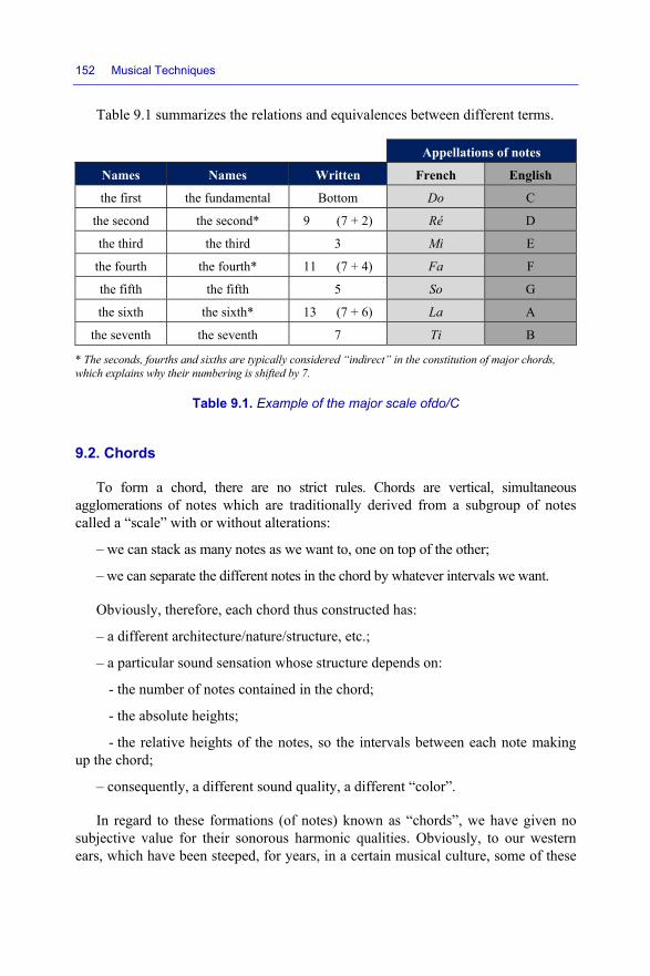
152 Musical Techniques
Table 9.1 summarizes the relations and equivalences between different terms.
Appellations of notes
Names Names Written French English
the first the fundamental Bottom Do C
the second the second* 9 (7 + 2) Ré D
the third the third 3 Mi E
the fourth the fourth* 11 (7 + 4) Fa F
the fifth the fifth 5 So G
the sixth the sixth* 13 (7 + 6) La A
the seventh the seventh 7 Ti B
* The seconds, fourths and sixths are typically considered “indirect” in the constitution of major chords, which explains why their numbering is shifted by 7.
Table 9.1. Example of the major scale ofdo/C
9.2. Chords
To form a chord, there are no strict rules. Chords are vertical, simultaneous agglomerations of notes which are traditionally derived from a subgroup of notes called a “scale” with or without alterations:
– we can stack as many notes as we want to, one on top of the other;
– we can separate the different notes in the chord by whatever intervals we want.
Obviously, therefore, each chord thus constructed has:
– a different architecture/nature/structure, etc.;
– a particular sound sensation whose structure depends on:
- the number of notes contained in the chord;
- the absolute heights;
- the relative heights of the notes, so the intervals between each note making up the chord;
– consequently, a different sound quality, a different “color”.
In regard to these formations (of notes) known as “chords”, we have given no subjective value for their sonorous harmonic qualities. Obviously, to our western ears, which have been steeped, for years, in a certain musical culture, some of these
Chords 153
chords “sound” good, others appear to be horrible aggregations of sounds (you may perfectly well lie your entire body across the keyboard of a piano to form a chord, but personally, I doubt the result will be “harmonic”, in any which way!).
For western ears, certain chord structures are recognizable. Once we have recognized them, we can catalog them, classify them, codify them, etc. With no pretense at being exhaustive, which is not the point of this book, it is this which we shall now recap in a few words.
Let us begin with the easiest of chords: firstly those which are made up of the simultaneous playing of three or four notes, and secondly those which are diatonics in the major scale.
RECAP.– Diatonic notes are notes which belong (solely) to the scale in question.
9.3. Diatonic chords
Again, let us take the simplest of examples to make our point.
For example, the diatonic chords in the major scale of do therefore are made up only of notes out of the seven notes of which the diatonic scale is intrinsically made up –i.e. do, ré, mi, fa, so, la and ti (to do so, suppose for a moment that someone has stolen all of the black keys off your piano). Remember that each note corresponds to a degree, so we have seven degrees.
Now that all these cumbersome black keys have (temporarily) been removed, running through the succession of notes in the above scale major degree by degree, and stacking up, by degrees, one note out of two, either in groups of three or in groups of four notes, we obtain series known as “diatonic chords”.
For instance, on the keyboard of a piano, maintaining the same position, the same spacing of the fingers on the hand and shifting the hand to the right or the left, we obtain:
– either chords formed of three notes which we call triads (see Table 9.2);
– or chords formed of four notes que we call seventh chords (also see Table 9.2).
In the same way as we number degrees and the position of the notes in a scale using “arabic numerals”, it was decided to number the different chords obtained above with “roman numerals” corresponding to the degree of the note to which the chord pertains.

154 Musical Techniques
Across the whole range of the C (do) major diatonic, scale, Table 9.2 shows the correspondence between the chord and its melodic content.
Example in the scale of do – C
N° of degree
N° of chord content of the 3-note chord content of the 4-note chord
1 I C E G C E G B
2 II D F A D F A C
3 III E G B E G B D
4 IV F A C F A C E
5 V G B D G B D F
6 VI A C E A C E G
7 VII B D F B D F A
Because there are only seven notes in the diatonic scale,and therefore seven degrees, there are initially only seven types of chords possible.
Table 9.2. Correspondence between the name of the chord and its melodic content in the scale of do
Now, let us examine the content of these chords in a little more detail.
9.3.1. Diatonic chords with 3 notes: “triads”
A three-note chord or triad is a chord formed of:
– a fundamental;
– a third, either minor (three semitones) or major (four semitones);
– a fifth.
In principle, these three notes also form a stack of thirds.
NOTE.– Generally, a chord containing three notes – a “triad” – is considered to be a simplified derivative of a four-note chord known as a “seventh” chord (see next section).
Table 9.3 shows an example of the types of triads contained in three-note chords in the scale of do major.

Chords 155
Triads contained in the chord (three-note chord)
degree n°
mode n°
degrees of the scale contained
in the chord
successive intervals
contained in the two triads
making up the chord
type of first triad contained
in the chord
type of chord obtained
1 I 1, 3, 5 M3 + m3 maj. triad maj. perfect chord
2 II 2, 4, 6 m3 + M3 triad min. min. perfect chord
3 III 3, 5, 7 m3 + M3 triad min. min. perfect chord
4 IV 4, 6, 1 M3 + m3 maj. triad maj. perfect chord
5 V 5, 7, 2 M3 + m3 maj. triad maj. perfect chord
6 VI 6, 1, 3 m3 + M3 triad min. min. perfect chord
7 VII 7, 2, 4 m3 + m3 triad dim. diminished chord
Table 9.3. Example of triads contained in the chords with three notes in the scale of do major
Figure 9.1. Representation in do major of the degrees on a scale
9.3.2. 4-note diatonic chords known as “seventh” chords”
A four-note chord or seventh chord is formed by superimposing a third on a three-note chord. The fourth note in that chord forms a seventh with the chord’s root note.
When the seventh of a four-note chord forms a dissonance with its fundamental, the chord is part of “dissonant harmony” (see examples later on: I M7 and IV M7).

156 Musical Techniques
Example of the types of triads contained in four-note chords known as seventh chords in the scale of do major are given below.
Triads contained in the 4-note so-called seventh chord
n° o
f the
deg
ree
type
of m
ode
mel
odic
con
tent
of t
he
chor
d tri
ad +
seve
nth
succ
essi
ve in
terv
als
cont
aine
d in
the
seve
nth
chor
ds
type
of t
he fi
rst t
riad
co
ntai
ned
in th
e se
vent
h ch
ord
nam
e of
the
seve
nth
chor
d
1 I 1, 3, 5 7 M3 + m3 + M3 maj. triad maj. seventh
2 II 2, 4, 6 1 m3 + M3 + m3 triad min. min. seventh
3 III 3, 5, 7 2 m3 + M3 + m3 triad min. min. seventh
4 IV 4, 6, 1 3 M3 + m3 + M3 maj. triad maj. seventh
5 V 5, 7, 2 4 M3 + m3 + m3 maj. triad dominant seventh
6 VI 6, 1, 3 5 m3 + M3 + m3 triad min. min. seventh
7 VII 7, 2, 4 6 m3 + m3 + M3 triad dim. diminished semi
Table 9.4. Triads contained in the four-note chord known as a seventh
Figure 9.2. Representation in do major of the degrees on a range
REMARKS PERTAINING TO THE LAST TWO TABLES.– Typically, we count the intervals which are present in triads or four-note chords, not from note to note, but in relation to the fundamental. Also in view of the fact that the sum of the intervals (M3 + m3) or (m3 + M3) is equal to a “perfect fifth – P5”, we could write that the maj. triad is formed of a M3 and a P5.
We have now listed the first “diatonic” chords formed, for example, simply by moving the same position of the hand on a piano keyboard.

Chords 157
9.4. “Fourth-based” chords
We showed earlier that the basic notes that characterize a chord formed with triads and then “enhanced with the seventh” are, harmonically, to begin with the fundamental and its fifth, followed by the third, and finally, the seventh, which gives the chord its “color”. However, many musicians value a different harmonic approach to that of third chords (triads), which are too predictable, and prefer chords (created) by (intervals of) fourths.
EXAMPLE.– A chord C F B instead of C E G B or C E♭ G B.
Note that in this chord [C F B], which includes a fourth, F, the major or minor color has disappeared (there is no longer a major third, with E, or a minor third, with E♭), and that the natural fifth of the fundamental (G) is no longer played.
The difficulty with these chords lies in the use of F in an Ionian major chord, although this note is that which sounds least good in the chord (because of the proximity of the B (ti) to the natural fifth of F (fa), which is the fundamental C (do)), which, in combination with the disappearance of the minor or major color, gives these chords a fuzzy, unstable nature. However, these chords are simply considered to be altered chords known as “suspended chords”, which are similar to normal triads (except for the fact that the third is replaced either by the major second “sus2”, or here by the fourth “sus4M”), and thus fit naturally into the logical harmonic of the descending chromaticism at the root of the sequences described in the next part of the book.
As regards purely diatonic chords containing four notes, there are many, many others which can be constructed around stacks containing second, fourth, augmented, diminished intervals, etc.
In short, it is up to you, the player, to decide on the combinations you wish to use.
9.4.1. Convention of notations of the chords
In general – but just in general! – the notations of chords are coded as follows.
For instance, a “C minor seventh minor and diminished sixth” would be written as Cm7 13b:
1) name of the fundamental;
2) “m” if the first third of the chord is minor;

158 Musical Techniques
3) “M7” if the seventh is natural, and “7” if the seventh is minor;
4) then, as needed, the name(s) of the altered degree(s) in order (often modulo 7).
The degrees are noted as follows, for instance in the scale of C major:
do ré mi fa so la Ti C D E F G A B
1 2 3 4 5 6 7 8 9 10 11 12 13 14
However, for chords in which the fifth is replaced by the sixth, the term 6 is used. For example, in a C6 chord, the G of the fifth is replaced by the A of the sixth.
ATTENTION.– Begging the pardon of purist, strict musicians (as we ourselves are… we can already hear their cries of protest!), for simple reasons of ease of writing and typography, all the chords presented in the rest of this book having alterations such as specific sharps or flats, depending on the scales in which they appear will be presented only as flats. For instance, an F# would be written as G♭.
It is certainly true that we are supposed to use a flat or a sharp on the altered note. A G♭ shows that the G is altered, whilst an F# refers to an altered F. Yet, for the purpose of simplifying the typing, programming and editing of computer files, we have preferred to use only flats. We could have an F# with an F in a scale. This changes nothing in terms of the type of chord used.
We thank readers for their understanding and indulgence!
9.5. Chord notations
NOTE.– For a color version of section 9.5, please see www.iste.co.uk/paret/ musical.zip.
Table 9.5 shows chords with very special forms. Indeed, they are all made up of 4 notes: their fundamental, their third, their fifth, possibly altered (augmented or diminished) in terms of minor thirds, seconds or fourths, and the seventh of the fundamental.
With the same fundamental, depending on the specific alterations of the thirds, fifths and sevenths, we note the four-note chords thus obtained in the form [fundamental, third, fifth, seventh], which generally gives us 6 main families of chords.
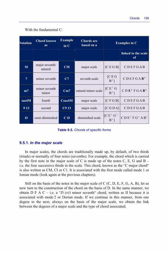
Chords 159
With the fundamental C:
Notation Chord known as
Example
in C Chords are based on a Examples in C
linked to the scale of
M major seventh/ natural CM major scale [C E G B] C D E F G A B
7 minor seventh C7 seventh scale [C E G B♭] C D E F G A B♭
m7 minor seventh minor Cm7 natural minor scale
[C E♭ G B♭] C D E♭ F G A B♭
sus4M fourth Csus4M major scale [C F G B] C D E F G A B
9 13 second C9 13 major scale [C G D A] C D E F G A B
Ø semi-diminished C Ø diminished scale [C E♭ G♭
B♭] C D E♭ F G♭ A B♭
Table 9.5. Chords of specific forms
9.5.1. In the major scale
In major scales, the chords are traditionally made up, by default, of two thirds (triads) or normally of four notes (sevenths). For example, the chord which is carried by the first note in the major scale of C is made up of the notes C, E, G and B – i.e. the four successive thirds in the scale. This chord, known as the “C major chord“ is also written as CM, CI or C1. It is associated with the first mode called mode 1 or Ionian mode (look again at the previous chapters).
Still on the basis of the notes in the major scale of C (C, D, E, F, G, A, B), let us now turn to the construction of the chord on the basis of D. In the same manner, we obtain D F A C – i.e. a “D (ré) minor seventh“ chord, written as II because it is associated with mode 2 or Dorian mode. If we continue in this manner, from one degree to the next, always on the basis of the major scale, we obtain the link between the degrees of a major scale and the type of chord associated.

160 Musical Techniques
major scale example in C: C D E F G A B N° of Name of the content of the chord name of
the chord degree mode mode chord in italics, the content and name of
the chord expressed in relation to C 1 I Ionian C1 C E G B D F A CM 1 3 5 7 9 11 13
2 II Dorian D2 D F A C E G B C2 C E♭ G B♭ D F A Cm7
3 III Phrygian E3 E G B D F A C C3 C E♭ G B♭ D♭ G A♭ Cm7
9♭ 13♭
4 IV Lydian F4 F A C E G B D C4 C E G B D F# A CM 11#
5 V Mixolydian G5 G B D F A C E C5 C E G B♭ D F A C7
6 VI Aeolien A6 A C E G B D F C6 C E♭ G B♭ D F G♭ Cm7 13♭
7 VII Locrian B7 B D F A C E G semi
diminished C7 C E♭ G♭ B♭ D♭ F A♭ CØ
ultimately, for the major scale, 7 degrees which correspond to the 7 possible chords
Table 9.6. Chords depending on the modes in the scale of do major
tone final chord
C D E F G A B C
CM C1 CM D2 Dm7 E3 Em7 F4 FM7 G5 G7 A6 Am7 B7 B Ø
To obtain the chord in question in a single octave, the notes shown in light grey lead to inversions of chord.
Table 9.7. Position of the fingers on a keyboard
Chords 161
The advantage to looking at the modes is that the chords always bear the same number (I to VII) or name whichever the fundamental used for the scale.
EXAMPLE.– The chord of E in the (diatonic) scale of D is a Dorian chord, and thus written in Em7.
Does this sound strange? Here is the explanation:
– the scale of D is formed of the notes D, E, F, G, A, B and C;
– its mode is Dorian;
– the first third in this scale of D is at F;
– that third is minor, so this scale is minor;
– in this scale of D, the chord formed by starting at E (second degree) will therefore be E, G, B, D, in which the first third, from E to G, is minor, the fifth from E to B is normal, and the distance from E to D represents a seventh;
– hence, this chord is written as an Em7.
Quite simple, is it not?
It is possible to use the same approach with all the chords in all the other scales. However, the tradition is to restrict harmonic rules to major and minor scales. Note that this choice is a little restrictive, particularly in the context of modern jazz, where more exotic scales (blues, bebop, etc.) are constantly used; however, the variety of types of chords available with the major or minor scale explains why the harmonic rules are limited to these scales, which (having a natural origin: the series of fifths) are therefore relatively well suited to carry harmony.
9.5.2. In minor scales
Let us immediately draw the distinction between four minor scales that are frequently used – e.g. in C (do):
– the “harmonic” minor scale, whose notes are C D E♭ F G A♭ B;
– the “natural” minor scale, whose notes are C D E♭ F G A B♭;
– the ascending “melodic” minor scale, whose notes are C D E♭ F G A B (this minor scale is most commonly used by jazz lovers, because it is closest to the major scale);
– the minor blues scale, whose notes are C D E♭ F F# G B♭.

162 Musical Techniques
9.5.2.1. In the “minor harmonic scale of C” (C D E♭ F G A♭ B)
harmonic minor scale example in C: C D E♭F GA♭ B
N° of Name of the content of the chord name of the chord
degree mode mode chord in italics, the content and name of the chord expressed in relation to C
C E G B D F A
1 3 5 7 9 11 13
1 I Ionian C1 C E♭ G B D F A♭ CmM 13♭
2 II D2 D F A♭ C E♭ G B
Locrian C2 C D♭ G♭ B♭ D♭ F A Cm7 5♭ 9 ♭
3 III E3 E♭ G B D F A♭ C
Ionian #5
C3 C E G# B D F A C 5#
4 IV F4 F A♭ C E♭ G B D
Dorian #11
C4 C E♭ G B♭ D G♭ A Cm7 11#
5 V G5 G B D F A♭ C E♭
Mixolydian 9♭ 13♭
C5 C E G B♭ D♭ F A♭ C7 9♭ 13♭
6 VI A6 A♭ C E♭ G B D F
Lydian 9# 11#
C6 C E G B D# F# A C 9# 11#
7 VII B7 B D F A♭ C E♭ G
diminished C7 C E♭ G♭ A D♭ E A♭ CØ
ultimately, for the major scale, 7 degrees which correspond to the 7 possible chords
Table 9.8. Chords depending on the modes in the harmonic minor scale of do

Chords 163
9.5.2.2. In the “natural minor scale of C” (C D E♭ F G A B♭)
The distribution of the intervals between notes is, in fact, none other than that which we find in the Dorian mode of a major scale of C (D E F G A B C).
natural minor scale example in C: C D E♭F G A B♭
N° of Name of the content of the chord name of the chord
degree mode mode chord in italics, the content and name of the chord expressed in relation to C
1 3 5 7 9 11 13
1 I Dorian C1 C E♭ G B♭ D F A Cm7
2 II Phrygian D2 D F A C E♭ G B♭
C2 C E♭ G B♭ D♭ F A♭ Cm7 9♭ 13♭
3 III Lydian E3 E♭ G B♭ D F A C
C3 C E G B D F# A CM 11#
4 IV Mixolydian F4 F A C E♭ G B♭ D
C4 C E G B♭ D F A C7
5 V Aeolien G5 G B♭ D F A C E♭
C5 C E♭ G B♭ D F G♭ Cm7 13♭
6 VI Locrian A6 A C E♭ G B♭ D F
demi diminished
C6 C E♭ G♭ B♭ D♭ F A♭ CØ
7 VII Ionian B7 B♭ D F A C E♭ G
C7 C E G B D F A CM ultimately, for the major scale, 7 degrees which correspond to the 7 possible chords
Table 9.9. Chords depending on the modes in the natural minor scale of do
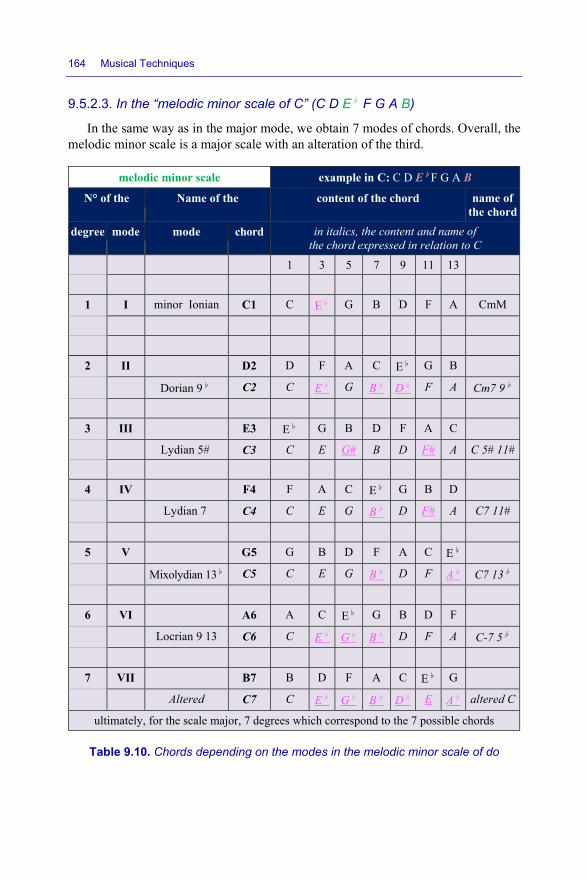
164 Musical Techniques
9.5.2.3. In the “melodic minor scale of C” (C D E♭ F G A B)
In the same way as in the major mode, we obtain 7 modes of chords. Overall, the melodic minor scale is a major scale with an alteration of the third.
melodic minor scale example in C: C D E♭F G A B
N° of the Name of the content of the chord name of the chord
degree mode mode chord in italics, the content and name of the chord expressed in relation to C
1 3 5 7 9 11 13
1 I minor Ionian C1 C E♭ G B D F A CmM
2 II D2 D F A C E♭ G B
Dorian 9♭ C2 C E♭ G B♭ D♭ F A Cm7 9♭
3 III E3 E♭ G B D F A C
Lydian 5# C3 C E G# B D F# A C 5# 11#
4 IV F4 F A C E♭ G B D
Lydian 7 C4 C E G B♭ D F# A C7 11#
5 V G5 G B D F A C E♭
Mixolydian 13♭ C5 C E G B♭ D F A♭ C7 13♭
6 VI A6 A C E♭ G B D F
Locrian 9 13 C6 C E♭ G♭ B♭ D F A C-7 5♭
7 VII B7 B D F A C E♭ G
Altered C7 C E♭ G♭ B♭ D♭ E A♭ altered C
ultimately, for the scale major, 7 degrees which correspond to the 7 possible chords
Table 9.10. Chords depending on the modes in the melodic minor scale of do

Chords 165
9.5.2.4. In the “minor blues scale of C” (C D E♭ F G♭ G B♭)
To conclude on the minor blues scale (the names of the blues modes are very variable from one piece of literature, so we shall content ourselves with indicating the name of the notes which make up the chord depending on the number of the mode). Note that F# is written as G♭ here.
minor blues scale example in C: C D E♭F G♭ G B♭ N° of Name of content of the chord name of the
chord degree mode mode chord in italics, the content and name of the chord
expressed in relation to C 1 3 5 7 9 11 13
1 I No particular
name
C1 C E♭ G♭ B♭ D F G C-7 5♭ 1 3 5 7 9 11 13
2 II D2 D F G C E♭ G♭ B♭ C2 C E♭ F A♭ D♭ E A♭ C-7 5 9♭
3 III E3 E♭ G♭ B♭ D F G C C3 C E♭ G B D E A CmM
4 IV F4 F G C E♭ G♭ B♭ D C4 C D G B♭ D♭ F A C7 3b♭ 9 ♭
5 V G5 G♭ B♭ D F G C E♭ C5 C E G# B C# F# A C 5# 9# 11#
6 VI A6 G C E♭ G♭ B♭ D F C6 C F G# B D# G A# CM 5# 9#
13#
7 VII B7 B♭ D F G C E♭ G♭ C7 C E G A D F G# CM 13# ultimately, for the scale major, 7 degrees which correspond to the 7 possible chords
Table 9.11. Chords depending on the modes in the minor blues scale of do

166 Musical Techniques
9.5.3. Scales and chords
9.5.3.1. Major scale
is linked to then the chord is it is a chord of the
type
C1 CM C D E F G A B C E G B D F A Δ
C2 BbM B♭ C D E♭ F G A C E♭ G B♭ D F A – 7
C3 AbM A♭ B♭ C D♭ E♭ F G C E♭ G B♭ D♭ F A♭ – 7 9♭ 13 ♭
C4 GM G A B C D E G♭ C E G B D G♭ A Δ #4
C5 FM F G A B♭ C D E C E G B♭ D F A 7
C6 EbM E♭ F G A♭ B♭ C D C E♭ G B♭ D F A♭ – 7 13♭
C7 DbM D♭ E♭ F G♭ A♭ B♭ C C E♭ G♭ B♭ D♭ F A♭
Ø or o: diminished semi
Table 9.12. Relations between scale and chords in the major scale
9.5.3.2. Minor harmonic scale
is linked
to then the chord is
it is a chord of the type
C1 Cm C D E♭ F G A♭ B C E♭ G B D F A♭ – M7 13♭
C2 Bbm B♭ C D♭ E♭ F G♭ A C E♭ G♭ B♭ D♭ F A – 7 5♭ 9 ♭
C3 Am A B C D E F A♭ C E A♭ B D F A Δ #5
C4 Gm G A B♭ C D E♭ G♭ C E♭ G B♭ D G♭ A – 7 #4
C5 Fm F G A♭ B♭ C D♭ E C E G B♭ D♭ F A♭ 7 9♭ 13 ♭
C6 Em E G♭ G A B C E♭ C E G B E♭ G♭ A Δ #9 #11
C7 Dbm D♭ E♭ E G♭ A♭ A C C E♭ G♭ A D♭ E A♭ diminished
Table 9.13. Relations between the scale and chords in the minor harmonic scale

Chords 167
9.5.3.3. Major blues scale
is linked to
then the chord is it is a chord of the type
C1 CBM C D E F G♭ G B♭ C E♭ G♭ B♭ D F G – 7 5♭
C2 BbBM B♭ C D E♭ E F A♭ C E♭ F B♭ D E A♭ – 7 5b♭ 13 ♭
C3 AbBM A♭ B♭ C D♭ D E♭ G♭ C D G♭ B♭ D♭ E♭ A♭ 7 9 5♭ 13 ♭
C4 GBM G A B C D♭ D F C D G B D♭ F A 9 ♭
C5 GbBM G♭ A♭ B♭ B C D♭ E C E A♭ B D♭ G♭ 5# 9 ♭ 13♭
C6 FBM F G A B♭ B C E♭ C F A B E♭ G B♭ m7
C7 DBM D E G♭ G A♭ A C C E G A D G♭ A♭ Δ
Table 9.14. Relations between the scale and chords in the major blues scale
9.5.3.4. Scale blues minor
is linked to then the chord is
it is a chord of the type
C1 CB C D E♭ F G♭ G B♭ C E♭ G♭ B♭ D F G – 7 5♭
C2 BbB B♭ C D♭ E♭ E F A♭ C E♭ F B♭ D♭ E A♭ – 7 5b♭ 9 ♭ 13♭
C3 AB A B C D E♭ E G C E♭ G B D E A – Δ
C4 GB G A B♭ C D♭ D F C D G B♭ D♭ F A 7 3b♭ 9 ♭
C5 GbB G♭ A♭ A B C D♭ E C E A♭ B D♭ G♭ A #5 9♭ 11 ♭
C6 FB F G A♭ B♭ B C E♭ C F A♭ B E♭ G B♭ #3 #5 #9 #13
C7 DB D E F G A♭ A C C E G A D F A♭ 13
Table 9.15. Relations between scales and chords in the minor blues scale
To supplement the tables above, Table 9.16 below looks at the four types of scales – major, minor, blues and whole-tone – and in degrees I, II, III, IV, V, VI and VII where they are located in their specific scales, listing the content of the chords whose fundamental frequency is a C.

168 Musical Techniques
Major scales on the basis of the scale of we obtain CM CD E F G A B C I C1 [ C E G B ] BbM B♭C D E♭ F G A C II C2 [ C E♭ G B♭ ] AbM A♭ B♭C D♭ E♭ F G CIII C3 [ C E♭ G B♭ ] GM G A B C D E G♭ C IV C4 [ C E G B ] FM F G A B♭C D E C V C5 [ C E G B♭ ] EbM E♭ F G A♭ B♭C D C VI C6 [ C E♭ G B♭ ] DbM D♭ E♭ F G♭ A♭ B♭C C VII C7 [ C E♭ G♭ B♭ ]
Minor scales on the basis of the scale de we obtain
Cm CD E♭ F G A♭ B C I C1 [ C E♭ G B ] Bbm B♭C D♭ E♭ F G♭ A C II C2 [ C E♭ G♭ B♭ ] Am A B CD E F A♭ CIII C3 [ C E A♭ B ] Gm G A B♭CD E♭ G♭ C IV C4 [ C E♭ G B♭ ] Fm F G A♭ B♭CD♭ E C V C5 [ C E G B♭ ] Em E G♭ G A B C E♭ C VI C6 [ C E G B ] Dbm D♭ E♭ E G♭ A♭ A C C VII C7 [ C E♭ G♭ A ]
Blues scales on the basis of the scale of we obtain
CB CD E♭ F G♭ G B♭ C I C1 [ C E♭ G♭ B♭ ] BbB B♭C D♭ E♭ E F A♭ C II C2 [ C E♭ F E♭ B♭ ] AB A B C D E♭ E G CIII C3 [ C E♭ G B ] GB G A B♭C D♭ D F C IV C4 [ C D G B♭ ] GbB G♭ A♭ A B C D♭ E C V C5 [ C E A♭ B ] FB F G A♭ B♭ B C E♭ C VI C6 [ C F A♭ B ] DB D E F G A♭ A C C VII C7 [ C E G A ]
Whole-tone scales
on the basis of the scale of we obtain CTT C D E G♭ A♭ B♭ C I C1 [ C E A♭ B♭ ] BbTT B♭C D E G♭ A♭ C II C2 [ C E A♭ B♭ ] AbTT A♭ B♭C D E G♭ CIII C3 [ C E G♭ B♭ ] GbTT G♭ A♭ B♭C D E C IV C4 [ C E G♭ B♭ ] ETT E G♭ A♭ B♭C D C V C5 [ C D G♭ B♭ ] DTT D E G♭ A♭ B♭C C VI C6 [ C D G♭ B♭ ]
Table 9.16. Content of chords whose fundamental frequency is a C in accordance to the types of scales

Chords 169
9.5.4. List of common chords
Chords are written in the form [fundamental, fifth, third, seventh].
C CM = [C G E B] C7 = [C G E B♭] Cm7 = [C G E♭ B♭] Csus4M = [C G F B] C913 = [C G D A] Co = [C G♭ E♭ B♭]
D♭ DbM = [D♭ A♭ F C] Db7 = [D♭ A♭ F B] Dbm7 = [D♭ A♭ E B] Dbsus4M = [D♭ A♭ G♭ C] Db913 = [D♭ A♭ E♭ B♭] Dbo = [D♭ G E B]
D DM = [D A G♭ D♭] D7 = [D A G♭ C] Dm7 = [D A F C] Dsus4M = [D A G D♭] D913 = [D A E B] Do = [D A♭ F C]
E♭ EbM = [E♭ B♭ G D] Eb7 = [E♭ B♭ G D♭] Ebm7 = [E♭ B♭ G♭ D♭] Ebsus4M = [E♭ B♭ A♭ D] Eb913 = [E♭ B♭ F C] Ebo = [E♭ A G♭ D♭]
E EM = [E B A♭ E♭] E7 = [E B A♭ D] Em7 = [E B G D] Esus4M = [E B A E♭] E913 = [E B G♭ D♭] Eo = [E B♭ G D]
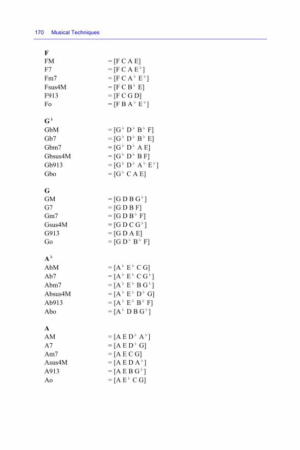
170 Musical Techniques
F FM = [F C A E] F7 = [F C A E♭] Fm7 = [F C A♭ E♭] Fsus4M = [F C B♭ E] F913 = [F C G D] Fo = [F B A♭ E♭] G♭ GbM = [G♭ D♭ B♭ F] Gb7 = [G♭ D♭ B♭ E] Gbm7 = [G♭ D♭ A E] Gbsus4M = [G♭ D♭ B F] Gb913 = [G♭ D♭ A♭ E♭] Gbo = [G♭ C A E] G GM = [G D B G♭] G7 = [G D B F] Gm7 = [G D B♭ F] Gsus4M = [G D C G♭] G913 = [G D A E] Go = [G D♭ B♭ F] A♭ AbM = [A♭ E♭ C G] Ab7 = [A♭ E♭ C G♭] Abm7 = [A♭ E♭ B G♭] Absus4M = [A♭ E♭ D♭ G] Ab913 = [A♭ E♭ B♭ F] Abo = [A♭ D B G♭] A AM = [A E D♭ A♭] A7 = [A E D♭ G] Am7 = [A E C G] Asus4M = [A E D A♭] A913 = [A E B G♭] Ao = [A E♭ C G]

Chords 171
B♭ BbM = [B♭ F D A] Bb7 = [B♭ F D A♭] Bbm7 = [B♭ F D♭ A♭] Bbsus4M = [B♭ F E♭ A] Bb913 = [B♭ F C G] Bbo = [B♭ E D♭ A♭] B BM = [B G♭ E♭ B♭] B7 = [B G♭ E♭ A] Bm7 = [B G♭ D A] Bsus4M = [B G♭ E B♭] B913 = [B G♭ D♭ A♭] Bo = [B F D A]
9.5.5. Table of frequently used chords
Table 9.17 shows the interval present in the most common chords.
# # # # # #
C D E F G A B C D E F G A
♭ ♭ ♭ ♭ ♭ ♭
number of degree 1 2 3 4 5 6 7 8 9 10 11 12 13
b3 b5 #5 b7
notation USA USA France
chords written in do
D T Q 7 7 9 11
d a d a m M
m3 M3 b5 P5 5+ M6 m7 M7
examples of formulations inAmerican notation

172 Musical Techniques
maj. triad I C C X X X
min. triad I - C- Cmin X X X
dim. triad I ° C0 Cdim X X X
aug. triad I + C+ C5+ X X X
fourth C4 C sus C sus X X
fourthsus C7 sus C sus7 X x) X X X X
maj. 6 I 6 C6 C6 X X x X
min. 6 I -6 C-6 Cm6 X X x X
dom. 7 I 7 C dom C7 X X X X
min. 7 I -7 C min 7 Cm7 X X X X
7 min 5 dim I -7(b5) C 07 Cm7/ 5- X X X X
7 dom 5aug I +7 C7/#5 C7/ 5+ X X X X
7 dom 5 dim I 7(b5) C7/b5 C7/ 5- 5 ♭ X X X X
7 dim I °7 Cdim7 X X X X
7 min 7 maj
I -M7 Cm maj7 Cm M7 X X X X
7 maj I M7 C maj7 CM7 X X X X
7 majaug I M7(#5) CM7(#5) X X X X
ninth C9 C9 C9 x X x) X X
ninthaug C+9 C #9 C9+ X x X X X X
ninth flat Cb9 C b9 C9 - X X X X X
ninth min Cm9 Cm 9 Cm9 X X X X X
eleventh C11 C11 X x) X X X X
eleventh aug C+11 C11+ X x) X X X X
thirteenth C13 C13 X X X X X X X
thirteenth flat
C-13 Cb13 C13 - X X X X X X X
Key: X obligatory note in the chord x optional note in the chord
Table 9.17. Standard nomenclature of chords (in do, C)
Almost all works in simple harmony include this type of table. So as not to omit this “monument of the profession”, here it is in Table 9.17.

Chords 173
Thus, everyone can construct their own “grids” because the content of the table shows how the chord is formed (in terms of intervals) in relation to the fundamental of the chord.
For the sake of ease, we have indicated the notations for a fundamental in “do – C”, but it is easy to “transpose” that table into other keys, without giving tons of chord grids for all the possible, imaginable tones, as is generally the case in many other books, merely for the pleasure of filling page space!
REMARK ON THE NOTATIONS USED IN THE TABLE.– The world of music is madly “artistic”, and there are a whole crowd of notations used to mean the same things (in actual fact, to speak of chords!). Therefore, do not be too critical in relation to the most common notations (both systems) which we have employed in this table, because there are many others which exist.
In a chord, taking the same notes contained in the chord in a different order, it is called a reversal.
9.6. What do these chords sound like?
To begin to determine how these chords “sound”, we first need to examine how they appear in terms of time, statically or dynamically – i.e. how the temporal relations between them are constructed. The next few paragraphs will go into detail about these two concepts.
9.6.1. In statics
A static chord is that which is played (“held down”) constantly on an instrument that is capable, by its construction, of maintaining the sound of each individual note in the chord (an organ, for instance).
In this case, we have the time to become aware of an individual chord, to imbibe it and note its intrinsic sonic color. This helps to train the ear in order to later easily recognize major chords, minor chords, seventh, seventh major chords, etc. Obviously, apart from this, what use can it truly have? Not much…!
9.6.2. In dynamics
Play a series of chords – a progression – and then it becomes a different story.

174 Mu
Obvifact that make no of soundHoweverseek to between temporalwill haveaspect of
The n
9.7. Tem
In dyand diffi
The mbegin wi
Figur
Our (frequenc
usical Technique
iously, if, betwthey succeedeffort (or at m
d to one another, if you are astick the piecthem (the pas
l and successie an impact onf the successio
next few parag
mporal relat
ynamics, timeicult to explain
Figuramplit
of this fig
musical sensaith the main on
re 9.3 gives a
brains’ instcy, amplitude,
es
ween two chord one another most a very mier and land yoa little quickerces together, st and the presive aspect (indn the auditory on of chords.
graphs will gi
tions betwee
e elapses and n in simple ter
re 9.3. 3D reprtude as a funcgure, please s
ation which wnes: frequency
simplified ex
tantaneous in, time) of these
rds, you wait in time, your
inimal one) to ou back, practir in the succeand try to fi
sent), or even dependently oimpression rec
ive further det
en chords
multiple pherms.
resentation of ction of melodysee www.iste.c
we perceive is y, time and am
ample using a
ntegration ofe parameters g
for a quarter r auditory memform the link
ically/almost, ession of the cind or construto predict and
of the pace of ceived. We the
tail on these tw
enomena occu
f frequency, timy. For a color vco.uk/paret/mu
linked to sevemplitude.
a 3D represent
f this three-gives us that w
of an hour, dmory (your bbetween the twin the previouchords, your buct harmonic d invent the fuf the successioen enter into a
wo concepts.
ur. All this is
me and version usical.zip
eral parameter
tation.
-dimensional well-known sen
espite the brain) will wo pieces
us section. brain will
relations uture! The on or not) a dynamic
complex
rs. Let us
response nsation of
Chords 175
musical wellbeing or unease. It is true that at any given time, we can examine the frequency content and, as a function of the time, we can examine the evolution of that frequency. This, though, is not enough. Our brains have an auditory memory, and sooner or later, acquires a musical education (whether wanted or not), which enables them, based on what has just happened, to predict, to invent what the next musical step could be. Distinguished mathematicians may note, in passing, that the way in which that musical peculiarity of the brain works, as a “function and convolution product” including the “delay theorem”, like any respectable phenomenon of convolution.
Thus, in dynamics, time elapses and various phenomena occur.
9.8. Melody line
A succession of (individual) notes played gives the ear the sensation of a melody, an air. It is the form of that melody which conveys an impression, a sensation of being in a particular tone, a particular mode. In addition to the main melody line, it is possible to add, in parallel, a bassline to complement and/or strengthen the main melody line.
9.9. Peculiarities and characteristics of the content of the chord
One of the main purposes of chords is to accompany and reinforce the melody. Furthermore, they serve to prepare the ground, to introduce and herald the next part of the melody. Therefore, the chord (usually) contains the notes which follow in the melody, but it may also be constructed so as to deliberately clash with the melody.
Thus, there is a direct and strong relation between the content of the melody line and the chords which are played along with it.
9.10. Relations between melodies and chords
Here too is one of the cornerstones of the premises of harmony.
Indeed, for something to be deemed harmonious, it must include very subtle nuances which the whole of our auditory apparatus (our ears, our brains, our education, etc.) is able to link together. We showed earlier that if the harmony is static – e.g. a chord played on its own and held – then in this case, the set of notes making it up must be harmonic, but also there must be relations between the harmonics which make up the chord and the ones which come before and after it. All of this will be discussed in detail in Part 4 of this book.

176 Musical Techniques
With regard to the dynamic aspect, there are time-dependent relations between the melodic content and the accompaniment line, for which there are various possibilities, as follows:
– the melody is accompanied instantaneously by notes that generally belong to the same tone or serve as a gateway chord, or which pave the way for a modulation, or a change of tone;
– the melodic content is preceded by accompanying notes which herald the next piece of the melody line (in fact, the notes in the melody played by the right hand will form part of the accompanying chords played very slightly before by the left hand);
– or the melody (mainly played by the right hand) invites certain notes and leads us, a little later on, to ensure the coherence of the harmonic ensemble perceived, and support it.
Hence the enigmatic quote: “everything which is in the right hand is, has been or will be in the left hand… and vice versa!” – a remark intended, obviously, for the players of keyboard instruments!
This subtle set of exchanges between the melody line and the accompaniment is permanent and, from a macroscopic point of view around a given moment in time, is regulated to around 2–3 measures before or after the corresponding melody.
9.11. The product of the extremes is equal to the product of the means
Here again is a very specialized field of study.
Indeed, following numerous physiological acoustic assessments, it has been found that our ears like to simultaneously hear either notes whose frequencies are fairly similar (e.g. in two neighboring octaves), or notes whose frequencies are at the high end and the low end of the spectrum. To express this idea numerically, i.e. in the audible frequency band from 20 to 20,000 Hz, we human beings prefer to simultaneously hear two average frequencies which are fairly close to one another (e.g. 300 and 600 Hz), or else two frequencies that are very far apart (e.g. 40 and 5000 Hz), rather than one medium note and one very low one (such as 500 and 40 Hz), or one medium and one very high (e.g. 500 and 8000 Hz). This leads us to conclude that there is an empirical law which, in the acoustic profession, is known as the “10-20,000 law”, or indeed the “20-10,000 law”, or even more simply, “product of extremes = product of means = 200,000”.
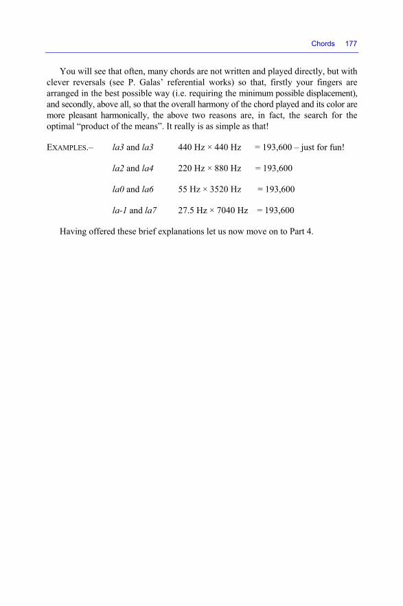
Chords 177
You will see that often, many chords are not written and played directly, but with clever reversals (see P. Galas’ referential works) so that, firstly your fingers are arranged in the best possible way (i.e. requiring the minimum possible displacement), and secondly, above all, so that the overall harmony of the chord played and its color are more pleasant harmonically, the above two reasons are, in fact, the search for the optimal “product of the means”. It really is as simple as that!
EXAMPLES.– la3 and la3 440 Hz × 440 Hz = 193,600 – just for fun!
la2 and la4 220 Hz × 880 Hz = 193,600
la0 and la6 55 Hz × 3520 Hz = 193,600
la-1 and la7 27.5 Hz × 7040 Hz = 193,600
Having offered these brief explanations let us now move on to Part 4.

PART 4
Harmonic Progressions
Introduction to Part 4
The objective in this fourth and final part is to provide readers with tools to help design harmonization grids for compositions and/or arrangements and for reharmonization of pieces of music, which can be used to create thousands of harmonic progressions! It is merely an aid – certainly a significant one – but there is no method which can substitute for a musician’s trained ear. However, the complexity of certain harmonic progressions (for example, in John Coltrane’s Giant Steps) shows how useful a little help can be, and that with a harmonic universe that is extremely rich, there is an infinity and an eternity of discoveries to be made.1
This part, initially based on a principle of 8 simple syntactic rules inspired by the theories of F. Pachet and M.J. Steedman (see bibliography) which, when taken together, give us the classic substitution progressions (II V I) and many more besides, has been reviewed and greatly enhanced by the principle of “descending chromatism”.
This part is concluded by applied examples of reharmonization of three well-known pieces of music: Blue Moon, Summertime and Sweet Georgia Brown, and the harmonization of a specific composition.
It must be remembered, though, that all of this is nothing without music, and that above all, “it must sound good”!
1 We would like to warmly thank all the teachers at the EDIM in Cachan, and in particular a few experts in harmony: Mônica Passos, Eric Shultz, Andrew Crocker and Daniel Beaussier.

10
Some Harmonic Rules
10.1. Definition of a chord and the idea of the color of a chord
As described at length in the previous chapters, a chord is defined by its fundamental, the fifth of the fundamental, the major or minor third, and the fifth of the third (the seventh), either major or minor. The constitutive notes in the chords form the primary color, whilst the other additional notes in those chords, whilst they are important in defining the chord, are ornamentations, and form a secondary/ additional color to the basic chord.
10.1.1. Notations used
All of the harmonic progressions presented in this and subsequent chapters are based on the types of chords introduced in the previous chapter, and therefore formed on the primary notes of the chords. For ease of notation and for reasons of simplification:
– chords are written in the order of a quartet [Fundamental, Third, Fifth, Seventh], and we add further alterations afterwards, but the harmonic rules pertain only to the basic quartet of the chord. For example, a G7 9b is primarily a G7 whose second is diminished;
– for the names of the chords, the English-speaking tradition is used from hereon in for the names of the notes in that quartet. For example, we have A for la, up to G for so;
– we use flat alterations instead of sharp alterations: for instance, a Gb instead of an F#. These simplifications are necessary so that we can more easily design a software tool to help study harmonic progressions and avoid repetitions (one section for F# and one for Gb).
Musical Techniques: Frequencies and Harmony, First Edition. Dominique Paret and Serge Sibony. © ISTE Ltd 2017. Published by ISTE Ltd and John Wiley & Sons, Inc.

184 Musical Techniques
In the next chapter, Harmonic progressions, we shall work mainly on the degrees of a given scale. The types of chords, therefore, will be directly defined by the degrees of the chord in the scale in question. However, for the application of the descending chromatism, we work on the basis of the quartet [Fundamental, Third, Fifth, Seventh]. The main reason for this choice lies in the fact that the fifth, the third and the fifth of the third are close harmonics of the fundamental, and therefore sound natural alongside it. In other words, the primary notes in the chord are the most powerful harmonics in terms of amplitude, which are, for most musical instruments, the basic quartet.
10.1.2. Equivalent or harmonious chords
Two chords can be considered equivalent (and therefore harmonious) if their constitutive quartets are equal or very similar, barring certain permutations.
For example:
– G7 is harmonious with CΔ because G7 is defined by [G, B, D, F], whilst CΔ is defined by [C E G B].
If we rearrange G7, we obtain [B D G B], which is the structure of CΔ with slight translations of the fundamental and the third of C. The greater these translations (or shifts), the less harmonious the two chords will be.
Two harmonious chords can be substituted for one another, or be played one after the other. We shall see later on that in fact, only descending translations of one or two notes within a chord can be used to switch from one chord to another. We therefore speak of descending chromatism, as defined in Chapter 11.
10.2. A few harmonic rules
Following an analysis of the sheet music in the “Real books” and other “Fake books”, we can formulate eight harmonic rules, which can be used for harmonic analysis of the different grids. Analyses of this type are presented in Chapter 11 of this book.
Far from being groundbreaking in the wonderful land of harmony, these rules are “known” to composers and rearrangers, but it is a good idea to recap them here:

Some Harmonic Rules 185
10.2.1. The eight fundamental syntactic rules
The eight fundamental syntactic rules used here are:
1) copying: any chord can be duplicated:
the chord sequence X Y → becomes X X Y
EXAMPLE.– Dm G7 CΔ → Dm Dm G7 CΔ
2) substitution to the tritone: for a maj 7 chord, if it is at the end of the progression or is followed by the fourth:
the chord X7 → can be substituted by Vb7
EXAMPLE.– Dm G7 CM → Dm Db7 CM
3) Dorian preparation: for a major 7 chord (considered a V Mixolydian chord), it is possible to add, before it, the II Dorian of that chord:
to the chord V7 → we can add IIm7 V7 to its left
EXAMPLE.– C7 G7 → C7 Dm7 G7
4) Mixolydian preparation: for a major chord M (considered a I Ionian chord), it is possible on the left to add the existing chord of a V Mixolydian of the chord:
to the chord I → we can add V7 I to its left
EXAMPLE.– Dm7 CM → Dm7 G7 CM
5) Lydian preparation: for a minor 7 chord (considered a II Dorian chord), it is possible to add the IV Lydian of the chord to the left:
IIm7 → IV7 IIm7
EXAMPLE.– Dm7 G7 → F7 Dm7 G7
6) destruction to the left: it is always possible to omit a chord in a progression; it becomes implicit:
X Y → Y
EXAMPLE.– Dm7 G7 CM → Dm7 CM
7) addition to the right of a fourth of the same type: any chord can be followed by its fourth with the same alteration:
X → X IV X
EXAMPLE.– C7 → C7 F7…
or Dm7 → Dm7 Gm7
186 Musical Techniques
8) addition, to the right, of a fifth of the same type: any chord can be followed by its fifth with the same alteration:
X Y → X V Y
EXAMPLE.– C7 Am7 → C7 G7 Am7
These last two rules are known as atonal, because they always force a change of key (tone), which the first six rules do not.
As western tradition is to respect the key (within the tritone), we shall pay more specific attention to the last two rules, which need to be taken within an overall progression which returns to the initial scale.
10.2.2. Rules of assembly
There are none! The eight rules set out above are, by definition, compatible, meaning that it is possible to apply these rules together and multiple times (on condition that we respect the types of chords specified in the rules (a “7” for the substitution to the tritone, for example). However, these rules are based on a fundamental progression to preserve a given color or mode.
Let us look at two examples:
1) the first illustrates a classic progression, starting at CΔ (CM) to return to CΔ (CM) (example: CΔ A7 Dm7 G7 CΔ) with the basic progression:
CΔ → CΔ
use of rule 4 (Mixolydian preparation) on the second CΔ:
CΔ G7 CΔ
use of rule 4 (Mixolydian preparation) on the G7:
CΔ D7 G7 CΔ
use of rule 4 (Mixolydian preparation) on the D7:
CΔ A7 D7 G7 CΔ
use of rule 6 (destruction) on the D7:
CΔ A7 G7 CΔ

Some Harmonic Rules 187
use of rule 3 (Dorian preparation) on the G7:
CΔ A7 Dm7 G7 CΔ
2) the second illustrates a turnaround
2 used by Bill Evans (CΔ Eb7 Ab7 Db7 CΔ) in CΔ starting from CΔ:
CΔ → CΔ
use of rule 4 (Mixolydian preparation) on the second CΔ:
CΔ G7 CΔ
use of rule 4 (Mixolydian preparation) on the G7:
CΔ D7 G7 CΔ
use of rule 4 (Mixolydian preparation) on the D7:
CΔ A7 D7 G7 CΔ
use of rule 2 (substitution to the Tritone) of the A7 (which resolves to D7):
CΔ Eb7 D7 G7 CΔ
use of rule 2 (substitution to the Tritone) of the D7 (which resolves to G7):
CΔ Eb7 Ab7 G7 CΔ
use of rule 2 (substitution to the Tritone) of the G7 (which resolves to C7):
CΔ Eb7 Ab7 Db7 CΔ
10.2.3. Next steps
In addition to, and in contrast to, solutions based on these eight rules, the chord progressions which we shall now present are complete, meaning that overall, they are coherent from the first to the last chord, and are based on the “descending chromatism” rule, which is only applied to the notes of the scale at hand – a subject which we shall examine in detail below. Indeed, for example, the rule of Mixolydian preparation of a major chord previously did not take account of the type of chord
2 Conventionally, in a harmonic progression, the term “Turnaround” refers to a series of chords (found in the same diatonic scale) placed at the end of a harmonic section. Its function is to create a form of tension (harmonic and/or melodic), which is resolved at the start of the next harmonic section (generally on the tonic chord in question).

188 Musical Techniques
situated before the major chord, and could, in some cases, lead to the addition of a 7th chord which is incompatible with that first chord.
10.2.4. Descending chromatism rule
The study of the great jazz pianists (Keith Jarrett, Bill Evans, Brad Mehldau, etc.) and detailed analysis of the sheet music in the editions of the Real Book, Aebersold Play-A-Long books, etc., which are known to all professionals and amateurs in jazz, shows that they all have the same approach to harmony which, moving around the scale of the key we are playing in, consists of the smallest possible shifts of the left hand, which typically forms the harmony – changing by a tone or a semitone at a time, which gives us the word “chromatism”.
This can be summarized simply as follows: two chords are considered to be “harmonically linked” if it is possible to move from the first defining quartet [fundamental, third, fifth, seventh] to the next one by descending chromatisms.
10.2.4.1. The why and wherefore of descending chromatisms
In our western physiological culture, the harmonic principle is to create/play (physical) sounds which are as natural as possible and avoid “friction” (or harshness or dissonance), which may be more or less marked, occurring when we play a note close to the natural harmonic (sub)-frequencies, but shifted by one degree in the scale (by a tone or a semitone). The presence of harmonics will sound natural, but when we play a similar note – but one whose value is not exactly equal to the harmonic – it will sound “wrong” or “harsh”.
Of course, there is an exception to every rule, including the rule on chromatism! The exception here is quite a significant one; it would be too easy otherwise! The exception in question is that of the “seventh”.
To explain this, let us take an example and explain the relations between the notes.
In the C major scale, play the chord CΔ, whose constitutive quartet is [C E G B]:
– C is the fundamental of the chord, with the frequency fo;
– E is major third of C, whose frequency is 5/4 × fo;
– G is the fifth of C, with frequency 3/2 × fo, and it is also the minor third of E;
– B is the fifth of E, with frequency 3/2 × (5/4 × fo), and at the same time the third of G, whose frequency is 5/4 × (3/2 × fo), is situated just below the fundamental.

Some Harmonic Rules 189
Although B is situated one degree (the value of a semitone) below C, meaning that the two notes are slightly dissonant, the harmonic effects – mainly of the fifth of E (the factor 3/2 of the fifth) and the third of G – emerge, and are stronger than the effect of the slight dissonance… and the chord sounds right!
On the other hand, the tritone of C, which is F#, always sounds horrendous, because it conflicts with the fifth of the fundamental, which is too close (namely G). The same is true for the minor second of C (C#), which sounds wrong, because it has no harmonic link other than with the fundamental. Thus, it appears that, even if ascending chromatisms are harmonically valid, they are less powerful than descending chromatisms. It is true that an ascending chromatism involves the octave and the minor second of the octave, and that this second is justified, because the fifth of the third of the minor second is the fundamental.
EXAMPLE.– The third of Db is F, whose fifth is C, so Db is linked to C, because the fifth of the third of Db is C!
However, in most cases, we play the chord of C (e.g. C E G B) and seek to carry out chromatisms on that basis. In such a case, it is very hard to justify the presence of a Db, because the chord Db is not constructed; only the note is played. Thus, we have a harmonic weakness, which can be used, but is weaker than the descending chromatism.
In summary, then, whilst it is harmonious to move from a note to its seventh (say, from C to B in the major scale, because the seventh is the fifth of the natural third of the note, as indicated above), it is disharmonious to move from a note to its minor second (C to Db), because Db is not linked to a harmonic of the note.
This simple observation justifies all eight rules of progression deriving from the simple rule of descending chromatism, but there are still exceptions to this rule. Indeed, if you go through a series of chords linked harmonically by descending chromatism, in principle, it is possible to use the same series of chords in the opposite direction, from the last to the first, through a mirror effect. The chromatism used is then opposite to the original one, and becomes an ascending chromatism. Hence, in principle, it should be possible to use ascending chromatisms, but only in symmetry with descending chromatisms. This alters nothing in terms of the harmonic quality of the chord changes, but this is justified by reference to the first series of chords linked by descending chromatism.
10.2.4.2. In conclusion
The descending chromatism rule applies only to the notes in the quartet of the initial chord [fundamental third fifth seventh]. Yet key changes in the current scale are free. However, the tradition in western music is to limit these key changes
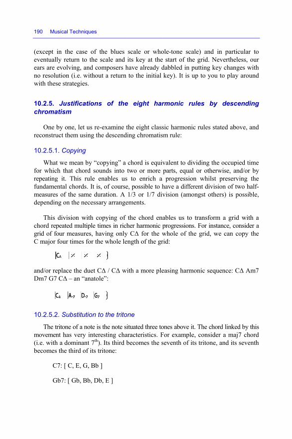
190 Mu
(except eventualears are no resoluwith thes
10.2.5. chroma
One reconstru
10.2.5.1
Whatfor whicrepeatingfundamemeasuresdependin
This chord repgrid of fC major
and/or reDm7 G7
10.2.5.2
The tmovemen(i.e. withbecomes
C
G
usical Technique
in the case olly return to thevolving, andution (i.e. witse strategies.
Justificatioatism
by one, let usuct them using
1. Copying
t we mean bych that chord g it. This rulental chords. Is of the same ng on the nece
division withpeated multipl
four measures,four times for
eplace the due7 CΔ – an “ana
2. Substitutio
tritone of a notnt has very inh a dominant 7s the third of it
C7: [ C, E, G, B
Gb7: [ Gb, Bb,
es
of the blues he scale and d composers hhout a return
ons of the
s re-examine tg the descendi
y “copying” a sounds into t
le enables usIt is, of course
duration. A essary arrange
h copying of le times in rich, having onlyr the whole le
et CΔ / CΔ wiatole”:
on to the trito
te is the note sinteresting cha7th). Its third bts tritone:
Bb ]
, Db, E ]
scale or whoits key at the
have already dto the initial
e eight har
the eight classing chromatis
chord is equivtwo or more to enrich a
e, possible to h1/3 or 1/7 div
ements.
the chord enaher harmonic p
y CΔ for the wngth of the gr
ith a more ple
ne
ituated three toaracteristics. Fbecomes the s
ole-tone scale start of the gdabbled in putkey). It is up
rmonic rule
sic harmonic rm rule:
valent to dividparts, equal oprogression
have a differenvision (among
ables us to trprogressions. Fwhole of the rid:
easing harmon
ones above it. TFor example, seventh of its
e) and in partgrid. Neverthetting key chanto you to pla
es by des
rules stated ab
ding the occupor otherwise, a
whilst presernt division of gst others) is
ransform a grFor instance, cgrid, we can
nic sequence:
The chord linkconsider a matritone, and it
ticular to eless, our nges with ay around
cending
bove, and
pied time and/or by rving the two half-possible,
rid with a consider a copy the
CΔ Am7
ked by this aj7 chord ts seventh

Some Harmonic Rules 191
The two chords are considered to be harmonically equivalent, so substitution is possible, which allows for or implies possibilities in terms of progressions.
There is only an inversion between the third and the seventh of the chord when switching to the tritone – hence the complicity between a chord and its tritone. However, the interval note/tritone is very disharmonious, because the fifth of the fundamental is very close to the tritone (Gb in the case of C), and therefore it is tricky to use a tritone (or even prohibited: it is known as “the Devil’s interval”). Often, we continue the movement to G or F in order to come back to a more “acceptable” chord.
In conclusion, the substitution above is possible when we start with a major chord:
CΔ: [ C, E, G, B ]
Gb7: [ Gb, Bb, Db, E ]
B drops to Bb, following a harmonic descending chromatism.
The same is not true, though, with a minor chord:
Cm7: [ C, Eb, G, Bb ]
Gb7: [ Gb, Bb, Db, E ]
Eb is not one of the notes characteristic of the Gb with the same alteration. Therefore, the chord does not work, and the progression is not possible.
10.2.5.3. Dorian preparation
The principles of third/seventh equivalence and of slight translations justify this rule:
Dm7: [ D, F, A, C ]
G7: [ G, B, D, F ]
The seventh of G7 is the third of Dm7: F.
The third of G7 is the descending seventh of Dm7: C goes to B.
Hence, the progression Dm7 G7 is harmonically possible.

192 Musical Techniques
10.2.5.4. Mixolydian preparation
The same principles are used to justify this rule:
G7: [ G, B, D, F ]
CΔ: [ C, E, G, B ]
The seventh of CΔ is the third of G7: B.
The third of the CΔ is the descending seventh of G7: F goes to E.
Thus, the progression G7 CΔ is harmonically possible.
10.2.5.5. Lydian preparation
The same principles are used to justify this rule:
F7: [ F, A, C, Eb ]
Dm7: [ D, F, A, C ]
The F A C belongs to both chords.
The Eb drops to the D.
Thus, the progression F7 Dm7 is harmonically possible.
Note that, in this case, the movement takes place through a simple descending semitone, which is also acceptable.
10.2.5.6. Destruction to the left
This rule is based on a hearer’s intuition, because the chord left out (at most one out of two) is, at best, reconstructed by the ear, and at worst, forgotten. This rule helps to lighten progressions which are too predictable.
10.2.5.7. Addition, to the right, of a fourth of the same type
A chord and its fourth are harmonically linked, as the chord is simply the fifth of the fourth. Indeed, the two chords share the same quartet (fundamental, third, fifth, seventh), after translations descending along the scale:
C7: Fundamental: C, Third: E, Fifth: G, Seventh: Bb
F7: Fundamental: F, Third: A, Fifth: C, Seventh: Eb

Some Harmonic Rules 193
Thus, the two chords are linked only by their common harmonic: the fifth of the fourth is the fundamental of the initial chord, and the seventh of the fourth is the third of the initial chord. This relation must therefore be respected by the couple third/seventh, which implies that the two chords must be of the same type (a Cm7 would be followed by an Fm7).
10.2.5.8. Addition, on the right, of a fifth of the same type
Same reasoning as for rule 7, but taking the fifth of the fundamental instead of the fifth of the fourth. Example:
C7: Fundamental: C, Fifth: G, Third: E, Seventh: Bb
G7: Fundamental: F, Fifth: C, Third: A, Seventh: F
10.3. Conclusions on harmonic rules
To conclude this short chapter, in order to continue a melody line or introduce a musical progression, so that two chords run together harmonically, the next chord simply needs to be made up of the notes of the first chord, with the exception of one or two simultaneous descending chromatisms, which is therefore necessary and sufficient to find the 8 harmonic rules, and this principle alone will suffice to construct all the progressions.
By way of progression, let us now move on to… harmonic progressions!

11
Examples of Harmonic Progressions
In the wake of the last chapter, where we set out the main rules that we intend to use, here now is a chapter on the detailed application of harmonic progressions by descending chromatism.
11.1. Harmonic progressions by descending chromatism
In order to fully comprehend the reasons why descending chromatism works and the harmonic progressions that can be created with this strategy, let us take as a reference example that which is conventionally based on the C major scale made up of the notes (C, D, E, F, G, A, B).
11.1.1. Example 1
In the scale of C: (C, D, E, F, G, A, B), in the Mixolydian mode, the notes in the quartet of a G5 chord, written as GV, or indeed G7, depending on the different types of notations used, are [ G, B, D, F ].
If, for example, we move two notes (D and F) in that chord by one degree of a descending chromatic movement – i.e. by moving D to C and F to E – we obtain a new chord [ G, B, C, E ].
This latter chord is, in fact, simply one of the possible inversions of the chord CΔ = [ C, E, G, B ] and it is harmonic because the new chord contains a major third, a fifth and the fifth of the third.
Thus, harmonically speaking, the chord GV = G7 can be followed by the CI chord (CΔ) with no friction and all with only a minimal movement of the fingers. This is what is known as Mixolydian preparation.
Musical Techniques: Frequencies and Harmony, First Edition. Dominique Paret and Serge Sibony. © ISTE Ltd 2017. Published by ISTE Ltd and John Wiley & Sons, Inc.

196 Musical Techniques
Table 11.1 gives the details, step by step, of the content of this maneuver from G7 to CΔ.
Degrees 1 2 3 4 5 6 7 Notes G A B C D E F G A B C
initial chord G7M or GV X x x
x
harmonic content of the initial chord
tonic
third major of the tonic
2 tones
fifth of the tonic
3 tones 1/2
fifth
of the third
frequency of the harmonic fo = fundamental × 5 × 3 × 7
in frequency fo = fundamental fo × 5/4 fo × 3/2 fo × 7/4 Descending chromatism X x x
D to C x F to E
final reorganized chord CΔ or CI
x x x x
harmonic content of the chord tonic
third major of the tonic
2 tones
fifth 3
tones 1/2
fifth of the third 3 tones
1/2
in frequency fo' = fundamental fo'×5/4 = fo" fo' × 3 fo" × 3
Table 11.1. Example: the path from G7 to CΔ. For a color version of this table, please see www.iste.co.uk/paret/musical.zip
Using this simple principle, we can work with all the major rules of harmony, e.g. passage in the Mixolydian, the Dorian, perfect cadence, etc.
11.1.2. Example 2
In the scale of C: (C, D, E, F, G, A, B), in the Dorian mode, the notes of a chord D2 = Dm7, depending on the different types of notations, are [ D, F, A, C ].
Carrying out a descending chromatism, A is linked to G, and C to B.

Examples of Harmonic Progressions 197
Thus, we obtain [ D, F, G, B ], which is the G7 chord out of order [ G, D, B, F ].
Dm7 can be followed by G7 which is Dorian preparation.
11.1.3. Example 3
In the scale of C: (C, D, E, F, G, A, B), the chord CΔ is [ C, G, E, B ].
Carrying out a descending chromatism, B is linked to A, so we obtain [ C, G, E, A ], which is the Am7 chord in the wrong order [ A, E, C, G ].
CΔ can be followed by Am7.
Once again, Table 11.2 shows the details of the path of the progression.
Degrees 1 2 3 4 5 6 7 Notes G A B C D E F G A B C
initial chord CΔ x x x x
harmonic content tonic
third major of the tonic
2 tones
fifth
3 tones 1/2
fifth of
the third
frequency fo = fundamental fo × 5/4 fo × 3/2 fo × 7/4
descending chromatism x x X x
reorganized x x x X
final chord Am7
tonic
third minor
of the tonic 1 tone 1/2
fifth
3 tones 1/2
fifth of
the third
frequency fo' = fundamental = fo" fo' × 3 fo" × 3
Table 11.2. Example: the path from CΔ to Am. For a color version of this table, please see www.iste.co.uk/paret/musical.zip

198 Musical Techniques
The ensemble and compilation of three detailed examples of preparations of series of chord using descending chromatism, which we have chosen to present above, ultimately gives the chord progression CΔ, Am7, Dm7, G7, CΔ, which, as it starts at a CΔ and returns to a CΔ, forms the classic progression known as “perfect cadence”, conventionally called “anatole”, or the progression written as (1) 6, 2, 5, 1 or VI II V I explained here with the simple principle of descending chromatism.
Table 11.3 gives an overview of the way of working.
N° Example: for the C major scale
of degree
of mode
name of mode Type of chord
content of the chord
name of the chord
reordered content
1 I Ionian M or maj or Δ
(C G E B) C1 CΔ C E G B
6 VI Aeolian m7 13b or min7 13b
(A C E G) A6 Am7 C E G A
2 II Dorian m7 (D F A C) D2 Dm7 C D F A
5 V Mixolydian 7 (G B D F) G5 G7 B D F G
1 I Ionian M or maj or Δ
(C G E B) C1 CΔ B C E G
Table 11.3. Classic progression known as “perfect cadence”
With each change/succession of a chord whose content has been reordered, only one or two fingers (indicated in bold) change position in relation to the previous chord to play the next one. On the keyboard of a piano, therefore, maintaining the harmony in the chord progression, the movement of the left hand playing the accompaniment is very slight.
11.2. Codes employed for writing progressions
NOTE.– For a color version of section 11.2, please see www.iste.co.uk/paret/ musical.zip.
Before going any further in this chapter, here are the codes which we shall use to codify (and decrypt) all of the tables and progression grids presented below.

Examples of Harmonic Progressions 199
In addition, these progression grids are sorted and classified depending on the number of chords making up the progressions and the name of the initial key of the chords.
The number shown in the first column is a note of assessment of the harmonious aspect of the progression. That number corresponds to the probability of finding that progression using the descending chromatism rule: the higher the note is (out of 100), the better the progression sounds. On the other hand, the more complex the progression, the less chance we have of finding it, and therefore its assessment note is lower.
The second number (second column) is the number of possible chords making up the progression (to avoid producing too weighty a tome, the maximum number of chords present in a progression has deliberately been limited to 14-15 chords for the most complex progressions, and can be reduced to 6 or 7 for the more conventional ones).
The purpose of the T in the third column is to indicate, at the start of the progression, the key or tone in which we start, or during the progression that a key change is going to take place.
Where we find a column showing the T, the next column indicates the (new) key of the scale to be used and its type (M major, m minor, B blues, TT whole tone) – a key which would then become that of the current scale.
Note that, for simplification purposes of the design of the composition-support software, the I degree of the scale, which is traditionally written as Δ, is also indicated by an M (for Major). A C major, often written as CΔ, is therefore represented as CM here.
Finally, the next column(s) give(s) a concrete list of the chords to be played.
N.B. The couples “notes – numbers” to be played, displayed after the key of the scale, correspond to their degrees in the scale at hand (see the detailed example later on).
For ease of writing, these numbers are given in Arabic numerals, whereas they should normally be presented in Roman numerals. For instance, where you see E3, read E III in the key of the scale in which we are playing (see example later on in this chapter).
11.2.1. Key changes in a progression
Here are a few important remarks on the subject of key changes.

200 Musical Techniques
Here and there, in numerous progressions, we see the appearance of a letter “T” which, as indicated above, corresponds to a key change during the progression. Indeed, a minor seventh “m7” chord may be a Dorian, a Lydian, a Phrygian, or even an Aeolian. Thus, several scales are available for the same chord, so there are possible (or necessary) key changes during the same series of chords (progression) in order to adapt to the melody. In this case, as indicated above, in the writing of the progression of the series of chords, the key change is indicated by the presence of the letter T, immediately followed by the new key to be applied to the new scale.
NOTE.– This point is important, because descending chromatism is carried out and must only be performed on the notes in the scale (major, minor, blues, whole-tone, etc.) at hand.
EXAMPLES.– As a function of the name of the chord following the letter T, the scales used thereafter in the progression are as follows:
T CM C D E F G A B T Cm C D Eb F G Ab B T CB C D Eb F Gb G Bb T CTT C D E Gb Ab Bb
T DbM Db Eb F Gb Ab Bb C T Dbm Db Eb E Gb Ab A C T DbB Db Eb E Gb G Ab B T DbTT Db Eb F G A B
T DM D E Gb G A B Db T Dm D E F G A Bb Db T DB D E F G Ab A C T DTT D E Gb Ab Bb C
T EbM Eb F G Ab Bb C D T Ebm Eb F Gb Ab Bb B D T EbB Eb F Gb Ab A Bb Db T EbTT Eb F G A B Db
T EM E Gb Ab A B Db Eb T Em E Gb G A B C Eb T EB E Gb G A Bb B D T ETT E Gb Ab Bb C D

Examples of Harmonic Progressions 201
T FM F G A Bb C D E T Fm F G Ab Bb C Db E T FB F G Ab Bb B C Eb T FTT F G A B Db Eb
T GbM Gb Ab Bb B Db Eb F T Gbm Gb Ab A B Db D F T GbB Gb Ab A B C Db E T GbTT Gb Ab Bb C D E
T GM G A B C D E Gb T Gm G A Bb C D Eb Gb T GB G A Bb C Db D F T GTT G A B Db Eb F
T AbM Ab Bb C Db Eb F G T Abm Ab Bb B Db Eb E G T AbB Ab Bb B Db D Eb Gb T AbTT Ab Bb C D E Gb
T AM A B Db D E Gb Ab T Am A B C D E F Ab T AB A B C D Eb E G T ATT A B Db Eb F G
T BbM Bb C D Eb F G A T Bbm Bb C Db Eb F Gb A T BbB Bb C Db Eb E F Ab T BbTT Bb C D E Gb Ab
T BM B Db Eb E Gb Ab Bb T Bm B Db D E Gb G Bb T BB B Db D E F Gb A T BTT B Db Eb F G A
Table 11.4. Scales in the progression as a function of the chord following the letter T

202 Musical Techniques
11.2.2. Detailed example of decoding of progressions
For instance, let us consider the case of the progression:
34 9 T CM C1 A6 F4 T BbM F5 T CM D2 B7 G5 E3 C1
Here is how to read it and decode it step by step:
34 is the note of assessment, out of 100, of the harmonious aspect of the progression presented.
9 means that it is a chord progression which has 9 chords.
T CM: we are starting in C major, CM.
C1 : 1st chord C1 or C I, so in CM, made up of the notes C, E, G, B, which form a CM.
A6: 2nd chord A6 or A VI, still in CM, made up of the notes A, C, E, G, which form an Am7.
F4 : 3rd chord F4 or F IV, still in CM, made up of the notes F, A, C, E, which form an FM9b.
T BbM: note that we are changing key to Bb major!
F5: 4th chord F5 or FV in the scale of BbM: it is made up of the notes F A C Eb, which form an F7.
T CM: N.B.: we are shifting back to the key of C major CM!
D2: 5th chord D2 or D II, so in CM, made up of the notes D, F, A, C, which form a Dm7.
B7: 6th chord B7 or B VII, so in CM, made up of the notes B, D, F, A, which form a Bm7.
G5: 7th chord G5 or G V, so in CM, made up of the notes G, B, D, F, which form a G7.
E3: 8th chord E3 or E III, so in CM, made up of the notes E, G, B, D, which form an Em7.
C1: 9th chord C1 or C I, so in CM, made up of the notes C, E, G, B, which form a CM.

Examples of Harmonic Progressions 203
Throughout this chapter, we shall present these progressions in table form, as follows:
key i.e. on a scale of
through a chord
indication of the degree of the
chord in the scale in question
formed of triads (with 4 notes!)
name of the
chord played
We start with a key of
CM C D E F G A B
C1 C D E F G A B C E G B CM A6 C D E F G A B A C E G Am7 F4 C D EF G A B F A C E FM9b
Key change to
BbM Bb C D Eb F G A
F5 Bb C D EbF G A F A C Eb F7
New key change to
CM C D E F G A B
D2 C D E F G A B D F A C Dm7 B7 C D E F G A B B D F A Bm7 G5 C D E F G A B G B D F G7 E3 C D E F G A B E G B D Em7 C1 C D E F G A B C E G B CM
Table 11.5. Detailed example of how to decode progressions
Table 11.6 shows the example (in light grey) of the position of the fingers on the keys of a keyboard to play that progression and demonstrates how little the fingers and hand move because of the phenomenon of descending chromatism (shown in dark grey) in the step-by-step progression of the chords.
key final chord
C D E F G A B C
CM C1 CM A6 Am7 F7 FM
BbM F5 Fa7 CM D2 Dm7
B7 Bm7 G5 G7 E3 Em7 C1 CM
Table 11.6. Position of the fingers on a keyboard to play this progression

204 Musical Techniques
11.3. Hundreds, thousands of substitution progressions…
In this chapter, you will find numerous lists of harmonic progressions, but for reasons of limitation of the number of pages and ease of use, the lists presented are only partial. However, PDFs are available showing complete progressions and in all keys. Note also that a software tool to help read these progressions will soon be available on IOS and MacOS. It is a good idea to check whether it is available yet from the App Store. Further information can also be obtained by e-mail: [email protected].
The series of progressions presented later on in this book are complete and coherent, meaning that the harmonic rule of descending chromatism is applied by taking into account the whole chords, unlike progressions which could be based solely on a restricted part of chords. Of course, it is always possible to leave out one or more chords from this series of progressions to obtain the maximum number of chords desired knowing that:
– conventionally, by habit, atonal chords, preceded by a T and a new key, are often the first to be omitted;
– it is customary to leave out as many chords from a progression as we wish; the harmonic rule of descending chromatism is no longer applied exactly, and the ear is left as the sole judge of the harmonic quality of the progression.
11.3.1. Major scale, the best of
The seven tables making up Table 11.7 illustrate a practical approach to the analysis of harmonic progressions. This means we can obtain progressions in successive steps. However, working with transposed, complete lists of progressions is still an infinitely more practical approach.
In order to describe this approach, each grid lists the chords and the degree harmonically close of the base chord in C, for each of the seven possible degrees of the scale. In addition, they are accompanied by a playability value, which represents the ease of finding a harmonic progression with the next chord. The maximum value 100 corresponds to direct relations via descending chromatisms, and after that we list the couples of chords which harmonize best with one another.

Examples of Harmonic Progressions 205
Playability from To Playability From to 100 C1 F4 95 C2 F5 87 C1 D2 83 C2 D3 81 C1 B7 76 C2 Bb1 77 C1 A6 73 C2 A7 67 C1 G5 64 C2 G6 57 C1 E3 54 C2 Eb4 48 C1 C1 45 C2 C2
Playability from To Playability From to
83 C3 F6 92 C4 Gb1 69 C3 Db4 82 C4 D5 67 C3 Bb2 79 C4 B3 63 C3 Ab1 75 C4 A2 56 C3 G7 64 C4 G1 48 C3 Eb5 55 C4 E6 41 C3 C3 48 C4 C4
Playability from To Playability From to
94 C5 F1 97 C6 F2 80 C5 D6 84 C6 D7 73 C5 Bb4 80 C6 Bb6 73 C5 A3 74 C6 Ab4 61 C5 G2 66 C6 G3 52 C5 E7 56 C6 Eb1 44 C5 C5 47 C6 C6
Playability from To
87 C7 F3 75 C7 Db1 70 C7 Bb6 65 C7 Ab5 57 C7 Gb4 50 C7 Eb2 41 C7 C7
Table 11.7. Practical approach to the analysis of harmonic progressions. For a color version of this table, please see www.iste.co.uk/paret/musical.zip

206 Musical Techniques
11.3.1.1. How to use these seven tables
Example of an application to Table 11.7:
– start with CM, which is a C1 on the C major scale;
– in the first premier table (light grey), take a couple of chords which sounds good: C1 to A6, with a score of 77 (no problem, because a playability value greater than 50 is good harmonically; it sounds good);
– we then look for what to put with the A6. We transpose by three semitones to C6, and look at the sixth table (dark grey);
– C6 sounds good with F2 with a score of 97. We come back to A6 by retransposing by a tone and a half. F2 becomes D2;
– we look for what to put with the D2. We transpose by a tone to C2 and take the second table (light grey);
– C2 sounds good with F5, with a score of 95. We come back to D2 by retransposing by a tone. F5 becomes a G5;
– we look for what to put with the G5. We transpose by a fifth to C5, and look at the fifth table (dark grey);
– C5 sounds good with F1, with a score of 94. We retranspose by a fifth and obtain a C1.
Using these seven tables, we find the anatole: C1 A6 D2 G5 C1, which translates to CM Am7 Dm7 G7 CM.
With these tables, we can also estimate the playability of the progression by weighting the playability of each couple by the score that the whole progression would have with playability values of 100. Here, we obtain:
77 97 95 94 100 67100 100 100 100
=× × × ×× × ×
That same approach can be applied to any progression.
Obviously, as pointed out at the start of this section, it is infinitely more practical to work with transposed, complete lists of progressions!
11.3.2. List of harmonious progressions
To begin with, based on the C Major scale, here are two simple examples of construction by descending chromatic progressions starting at a C1 in CM, and always returning in CM to a C1.

Examples of Harmonic Progressions 207
11.3.2.1. First example, known as “perfect cadence or rhythm changes”
in the scale of CM C1 C E G B
we descend B C E G A
we obtain A6, which, in the scale of CM, is written A C E G
then we descend E and G A C D F
we obtain D2, which, in the scale of CM, is written D F A C
then we descend A and C D F G B
we obtain G5, which, in the scaleof CM, is written G B D F
then we descend D and F G B C E
we obtain C1, which, in the scale of CM, is written C E G B
Table 11.8. Harmonious descending-chromatism progressions
Thus, ultimately, in the key of CM, starting and ending at C1, we have a progression of five successive chords C1 A6 D2 G5 C1 (this is the progression numbered 82 in the list below).
key i.e. on a scale of
through a chord
indication of the degree of the
chord in the scale in question
formed of triads (with 4 notes)
name of the
chord played
We find ourselves in a key of
CM C D E F G A B C1 C D E F G A B C E G B CM
A6 C D E F G A B A C E G Am7
D2 C D E F G A B D F A C Dm7
G5 C D E F GA B G B D F G7
C1 CD E F G A B C E G B CM
Table 11.9. Summary. For a color version of this table, please see www.iste.co.uk/paret/musical.zip

208 Musical Techniques
11.3.2.2. Second example, known as “passage to the tritone”
We start in the scale of CM C1 C E G B We move to the scale of GM: T GM
We descend the G and B The descent from G to Gb gives the tritone interval from C to Gb C E GbA
we obtain Gb7 (GM) Gb A C E
We return to the scale of CM: T CM
Then we descend the Gb F A C E we obtain F4(CM) F A C E
Then we descend the C and E F A BD we obtain B7 (CM) B D F A
Then we descend the A B D F G we obtainG5(CM) G B D F
Then we descend the D and F G B CE we obtain C1 (CM) C E G B
Table 11.10. An alternative to the first example. For a color version of this table, please see www.iste.co.uk/paret/musical.zip
Thus, ultimately, starting in the key of CM, after passing through GM and returning to CM, we have an overall progression of 6 chords T CM C1 T GM Gb7 T CM F4 B7 G5 C1 and two key changes (this is the progression numbered 53 in the list below).
key i.e. on a scale of
through a chord
indication of the degree of the chord in the
scale in question
formed of triads (with 4 notes)
name of the
chord played
We find ourselves in a key of
CM C D E F G A B C1 C D E F G A B C E G B CM
Keychangeto GM G A B C D E Gb
Gb7 G A B C D E Gb
Gb A C E
Gbo
New key change to
CM C D E F G A B F4 C D EFG A B F A C E F7 B7 C D E F G A B B D F A Bo G5 C D E F GA B G B D F G7 C1 C D E F G A B C E G B CM
Table 11.11. Summary. For a color version of this table, please see www.iste.co.uk/paret/musical.zip

Examples of Harmonic Progressions 209
11.3.2.3. Examples of harmonious progressions
The approach suggested at the presentation of the seven tables above is functional, but is not able to directly give progressions, going from a given chord to another. For this, we need to move step by step, and continually transpose/retranspose, which renders the technique somewhat complex – hence the usefulness of drawing up systematic lists of progression in which we merely need to look up the couple of chords – “start, end” – to be studied. We then obtain a list (see ebooks) that is much more practical to use: one for each type of scale (major, minor, blues, whole-tone).
Following the two (simple) examples discussed above, let us put them into practice!
Using the same type of structure, e.g. on the scale C Major (CM) scale, from CM to CM and starting at C1 and returning to C1, here is the complete reproduction of the numerous tables and grids of progressions which sound good.
EXAMPLE OF A LIST.–
on the basis of the scale CM : C D E F G A B
search for chromatisms starting from C : [ C G E B ], which is a C1
to
on the basis of the scale CM: C D E F G A B
C: [ C G E B ], which is a C1
Table 11.12 deliberately sheds light on the chord changes throughout the proposed harmonic progressions, and the playability scores indicated in these lists, which are different to those composed with the above seven tables, because in these lists the standard of measurement is different and corresponds to the probability of obtaining the progression in its entirety with only the descending chromatism rule.
Table of chord progressions
100 5 T CM C1 F4 B7 G5 C1
82 C1 A6 D2 G5 C1
79 C1 F4 B7 E3 C1
74 C1 F4 D2 G5 C1
58 6
C1 A6 F4 B7 G5 C1
53 C1 T GM Gb7 T CM F4 B7 G5 C1
51 C1 A6 D2 B7 G5 C1
51 C1 F4 B7 G5 E3 C1

210 Musical Techniques
51 C1 F4 D2 B7 G5 C1
49 C1 T FM C5 T CM F4 B7 G5 C1
41 C1 T FM C5 T CM F4 D2 G5 C1
40 C1 A6 F4 B7 E3 C1
40 C1 A6 F4 D2 G5 C1
39 C1 F4 D2 B7 E3 C1
39 C1 F4 D2 G5 E3 C1
39 C1 T GM Gb7 T CM F4 D2 G5 C1
38 C1 A6 T GM D5 T CM D2 G5 C1
38 C1 T FM C5 T CM F4 B7 E3 C1
37 C1 A6 D2 B7 E3 C1
37 C1 T GM Gb7 T CM F4 B7 E3 C1
36 C1 A6 D2 G5 E3 C1
36 C1 A6 T BbM F5 T CM D2 G5 C1
35 C1 F4 B7 G5 T DM Db7 T CM C1
31 C1 F4 T BbM F5 T CM B7 G5 C1
28 C1 F4 T BbM F5 T CM D2 G5 C1
26 C1 F4 B7 T AM E5 T CM E3 C1
26 C1 F4 T BbM F5 T CM B7 E3 C1
26 C1 T FM C5 T CM A6 D2 G5 C1
25 C1 A6 D2 G5 T DM Db7 T CM C1
25 C1 A6 D2 T EbM D7 T CM G5 C1
25 C1 F4 D2 G5 T DM Db7 T CM C1
25 7 C1 A6 T GM D5 T CM D2 B7 G5 C1
24 6
C1 F4 B7 E3 T DM Db7 T CM C1
24 C1 F4 D2 T EbM D7 T CM G5 C1
24 7 C1 A6 F4 D2 B7 G5 C1
24 C1 F4 D2 B7 G5 E3 C1
24 C1 T GM Gb7 T CM F4 B7 G5 E3 C1
24 C1 T GM Gb7 T CM F4 D2 B7 G5 C1
23 C1 A6 D2 B7 G5 E3 C1
23 C1 T FM C5 T CM F4 B7 G5 E3 C1
23 C1 T FM C5 T CM F4 D2 B7 G5 C1
22 C1 A6 F4 B7 G5 E3 C1
22 C1 A6 T BbM F5 T CM D2 B7 G5 C1
20 C1 A6 T BbM F5 T CM D2 B7 E3 C1
19 C1 A6 F4 D2 B7 E3 C1
C1 T FM C5 T CM F4 D2 G5 E3 C1
C1 T GM Gb7 T CM F4 D2 B7 E3 C1
C1 T GM Gb7 T CM F4 D2 G5 E3 C1
18 C1 A6 F4 D2 G5 E3 C1
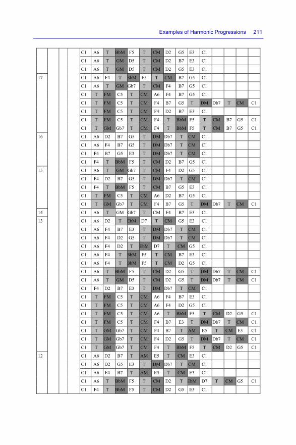
Examples of Harmonic Progressions 211
C1 A6 T BbM F5 T CM D2 G5 E3 C1
C1 A6 T GM D5 T CM D2 B7 E3 C1
C1 A6 T GM D5 T CM D2 G5 E3 C1
17 C1 A6 F4 T BbM F5 T CM B7 G5 C1
C1 A6 T GM Gb7 T CM F4 B7 G5 C1
C1 T FM C5 T CM A6 F4 B7 G5 C1
C1 T FM C5 T CM F4 B7 G5 T DM Db7 T CM C1
C1 T FM C5 T CM F4 D2 B7 E3 C1
C1 T FM C5 T CM F4 T BbM F5 T CM B7 G5 C1
C1 T GM Gb7 T CM F4 T BbM F5 T CM B7 G5 C1
16 C1 A6 D2 B7 G5 T DM Db7 T CM C1
C1 A6 F4 B7 G5 T DM Db7 T CM C1
C1 F4 B7 G5 E3 T DM Db7 T CM C1
C1 F4 T BbM F5 T CM D2 B7 G5 C1
15 C1 A6 T GM Gb7 T CM F4 D2 G5 C1
C1 F4 D2 B7 G5 T DM Db7 T CM C1
C1 F4 T BbM F5 T CM B7 G5 E3 C1
C1 T FM C5 T CM A6 D2 B7 G5 C1
C1 T GM Gb7 T CM F4 B7 G5 T DM Db7 T CM C1
14 C1 A6 T GM Gb7 T CM F4 B7 E3 C1
13 C1 A6 D2 T EbM D7 T CM G5 E3 C1
C1 A6 F4 B7 E3 T DM Db7 T CM C1
C1 A6 F4 D2 G5 T DM Db7 T CM C1
C1 A6 F4 D2 T EbM D7 T CM G5 C1
C1 A6 F4 T BbM F5 T CM B7 E3 C1
C1 A6 F4 T BbM F5 T CM D2 G5 C1
C1 A6 T BbM F5 T CM D2 G5 T DM Db7 T CM C1
C1 A6 T GM D5 T CM D2 G5 T DM Db7 T CM C1
C1 F4 D2 B7 E3 T DM Db7 T CM C1
C1 T FM C5 T CM A6 F4 B7 E3 C1
C1 T FM C5 T CM A6 F4 D2 G5 C1
C1 T FM C5 T CM A6 T BbM F5 T CM D2 G5 C1
C1 T FM C5 T CM F4 B7 E3 T DM Db7 T CM C1
C1 T GM Gb7 T CM F4 B7 T AM E5 T CM E3 C1
C1 T GM Gb7 T CM F4 D2 G5 T DM Db7 T CM C1
C1 T GM Gb7 T CM F4 T BbM F5 T CM D2 G5 C1
12
C1 A6 D2 B7 T AM E5 T CM E3 C1
C1 A6 D2 G5 E3 T DM Db7 T CM C1
C1 A6 F4 B7 T AM E5 T CM E3 C1
C1 A6 T BbM F5 T CM D2 T EbM D7 T CM G5 C1
C1 F4 T BbM F5 T CM D2 G5 E3 C1

212 Musical Techniques
C1 T FM C5 T CM A6 D2 G5 E3 C1
C1 T FM C5 T CM A6 T GM D5 T CM D2 G5 C1
C1 T FM C5 T CM F4 B7 T AM E5 T CM E3 C1
C1 T FM C5 T CM F4 D2 G5 T DM Db7 T CM C1
C1 T FM C5 T CM F4 T BbM F5 T CM B7 E3 C1
C1 T FM C5 T CM F4 T BbM F5 T CM D2 G5 C1
C1 T GM Gb7 T CM F4 T BbM F5 T CM B7 E3 C1
8 C1 A6 F4 D2 B7 G5 E3 C1
11
7 C1 A6 D2 B7 E3 T DM Db7 T CM C1
C1 A6 T GM D5 T CM D2 T EbM D7 T CM G5 C1
C1 F4 D2 B7 T AM E5 T CM E3 C1
C1 F4 D2 G5 E3 T DM Db7 T CM C1
C1 F4 D2 T EbM D7 T CM G5 E3 C1
C1 F4 T BbM F5 T CM B7 G5 T DM Db7 T CM C1
C1 F4 T BbM F5 T CM D2 B7 E3 C1
C1 T FM C5 T CM F4 D2 T EbM D7 T CM G5 C1
C1 T GM Gb7 T CM F4 B7 E3 T DM Db7 T CM C1
C1 T GM Gb7 T CM F4 D2 T EbM D7 T CM G5 C1
10 C1 T FM C5 T CM A6 D2 B7 E3 C1
8 C1 A6 T BbM F5 T CM D2 B7 G5 E3 C1
C1 T FM C5 T CM F4 D2 B7 G5 E3 C1
C1 T GM Gb7 T CM F4 D2 B7 G5 E3 C1
Table 11.12. Table of chord progressions. For a color version of this table, please see www.iste.co.uk/paret/musical.zip
Table 11.2 shows the great many progressions possible just on the C Major (CM) scale, from CM to CM, and starting at C1 before returning to C1. It must be kept in mind that the same is true for all other keys and types of scales and it is simply beyond the scope of this book to publish them all here.
11.3.2.4. Irreducible progressions
As indicated earlier, in all the tables presented here, deeming that it was sufficient in terms of the calculation, we have arbitrarily set ourselves a maximum value (a limitation) of 14 chords per progression. In this context, it should be noted that for certain couples of chords (such as moving from C3 to Db7 for instance), it is impossible to find a harmonious series of progressions. To resolve this type of change, therefore, we need to use an additional intermediary chord in order to find a suitable progression.

Examples of Harmonic Progressions 213
EXAMPLE OF THE MOVE FROM C3 TO DB7.– Let us take the example of the passage from C3 to Db7. In this case, we can go through the intermediary chord F5, for example, as follows:
– we make a first step from C3 to F5;
– then, we take a second step from F5 to Db7.
We then obtain and choose, for example, for C3 to F5:
100 2 T AbM C3 T BbM F5
Then, we search through the (lengthy) lists for the link between F5 and Db7:
100 5 T BbM F5 T CM D2 B7 T DM E2 Db7 78 5 T BbM F5 T CM D2 G5 T DM E2 Db7 44 4 T BbM F5 T CM D2 G5 T DM Db7 44 6 T BbM F5 T CM D2 B7 G5 T DM E2 Db7 33 5 T BbM F5 T CM D2 B7 E3 T DM Db7 33 6 T BbM F5 T CM D2 T EbM D7 T CM G5 T DM E2 Db7 22 6 T BbM F5 T CM D2 B7 T AM E5 T DM E2 Db7
We choose to use the first solution in this list:
100 5 T BbM F5 T CM D2 B7 T DM E2 Db7
Thus, we can deduce the final progression:
6 T AbM C3 T BbM F5 T CM D2 B7 T DM E2 Db7
The principle, then, is to arbitrarily place an intermediary chord to link the two parts of the sequence, before and after it.
Fortunately, such cases are very rare and we can almost always find a result by looking for progressions.
11.4. Chromatism in “standards”
Let us return now to the case of chromatisms. When we closely examine the progressions typically used in jazz standards (e.g. those presented in the Real Book), we see that the king of the progressions is the descending chromatism. By extension, we find symmetrical progressions (retracing the harmonic path in the opposite direction) which by its principle gives rise to ascending chromatisms but each time

214 Musical Techniques
we use a progression by ascending chromatism it is associated with an equivalent path in descending chromatism.
Let us give some examples:
From CM to CM
3 CM B7 CM Descending and then ascending 4 CM FM GM CM Descending and then ascending 5 CM Am7 Dm7 G7 CM Anatole so descending 6 CM Eb7 AbM Dm7 G7 CM Anatole prepared by the E, so
descending 7 CM Dm7 Em7 FM Em7 Dm7 CM Ascending and then descending 8 CM Bo E7 Am7 D7 Dm7 G7 CM Anatole a little atonal so descending 9 CM A7 Dm7 G7 Em7 A7 Dm7 G7 CM Double anatole so descending
From CM to C7
3 CM Gm7 C7 Ascending and then descending 4 CM FM Gm7 C7 Descending and then ascending 5 CM FM G7 CM C7 6 CM Gb7 Cm7 F7 Gm7 C7 7 CM Ebm7 Ab7 Dm7 G7 Gm7 C7 8 CM Eb7 AbM B7 EM G7 Gm7 C7 9 CM Gm7 C7 FM Fm7 Bb7 CM Gm7 C7
From CM to Cm7
3 CM Gb7 Cm7 4 CM Em7 Am7 Cm7 5 CM Gm7 C7 FM Cm7 6 CM D7 Bb7 C7 Gb7 Cm7 7 CM Dm7 Em7 F7 Cm7 F7 Cm7 8 CM Dbm7 Gb7 Ebm7 Ab7 Dbm7 Gb7 Cm7 9 CM Dm7 Em7 A7 Ebm7 Ab7 Dm7 G7 Cm7
11.5. Families of descending chromatisms
After a lengthy auditory verification of all these progressions, the next few paragraphs present a minimal/reduced portion of the results of the work done on descending harmonics, depending on the different keys of CM (scale major), Cm (minor scale), CB (blues scale), CTT (whole-tone scale) and give results classified by the number of descending chromatisms used to move from one chord to the next.

Examples of Harmonic Progressions 215
NOTES.– To validate or invalidate a type of progression, we are particularly interested in the anatole’s being present and correctly placed.
The anatole is a harmonic series.
The anatole on two measures is the following succession of chords: | I VI | II V |
For example, in the key of CM7: | C Am7 | Dm7 G7 |
The anatole can also be divided into 32 measures.
The turnaround is a group of two measures situated at the end of a phrase of eight measures, leading in to the repetition of that phrase. It is true that we commonly play a variant of anatole at that point, but the term turnaround more specifically indicates a place within the piece of music.
IMPORTANT NOTE.– In order to avoid uselessly overfilling this book, we have deliberately truncated the presentation of lists of progressions to around ten lines each, showing the most meaningful ones at the top of the lists, and the less significant ones at the bottom, just to give you an idea. As an addition, to obtain complete lists for each type of scale, you can send a request to [email protected].
11.5.1. Family: “1 chromatism at a time”
Let us begin by examining the family of progressions where we make a single descending chromatism at a time to move from one chord to the next.
11.5.1.1. In the major scale
No chromatism of the fundamental:
100 8 T CM C1 A6 F4 D2 B7 G5 E3 C1 34 9 T CM C1 A6 F4 T BbM F5 T CM D2 B7 G5 E3 C1 33 9 T CM C1 A6 F4 D2 B7 G5 E3 T DM Db7 T CM C1 33 9 T CM C1 A6 T GM Gb7 T CM F4 D2 B7 G5 E3 C1 33 9 T CM C1 T FM C5 T CM A6 F4 D2 B7 G5 E3 C1 11 10 T CM C1 A6 F4 T BbM F5 T CM D2 B7 G5 E3 T DM Db7 T CM C1 11 10 T CM C1 A6 T GM Gb7 T CM F4 D2 B7 G5 E3 T DM Db7 T CM C1 11 10 T CM C1 A6 T GM Gb7 T CM F4 T BbM F5 T CM D2 B7 G5 E3 C1 11 10 T CM C1 T FM C5 T CM A6 F4 D2 B7 G5 E3 T DM Db7 T CM C1 11 10 T CM C1 T FM C5 T CM A6 F4 T BbM F5 T CM D2 B7 G5 E3 C1

216 Musical Techniques
In the first line, anatole is indeed present but is lost in other transitionary chords: C1 A6 F4 D2 B7 G5 E3 C1.
Chromatism possible for the fundamental:
100 8 T CM C1 A6 F4 D2 B7 G5 E3 C1 34 9 T CM C1 A6 F4 D2 B7 G5 E3 T DM Db7 T CM C1 34 9 T CM C1 A6 T GM Gb7 T CM F4 D2 B7 G5 E3 C1 33 9 T CM C1 A6 F4 T BbM F5 T CM D2 B7 G5 E3 C1 33 9 T CM C1 T FM C5 T CM A6 F4 D2 B7 G5 E3 C1 12 10 T CM C1 A6 F4 T BbM F5 T CM D2 B7 G5 E3 T DM Db7 T CM C1 11 10 T CM C1 A6 T GM Gb7 T CM F4 D2 B7 G5 E3 T DM Db7 T CM C1 11 10 T CM C1 A6 T GM Gb7 T CM F4 T BbM F5 T CM D2 B7 G5 E3 C1 11 10 T CM C1 T FM C5 T CM A6 F4 D2 B7 G5 E3 T DM Db7 T CM C1 11 10 T CM C1 T FM C5 T CM A6 F4 T BbM F5 T CM D2 B7 G5 E3 C1
No particular gain in relation to the version without chromatism of the fundamental.
11.5.1.2. In the minor scale
No chromatism of the fundamental:
100 8 T Cm C1 Ab6 F4 D2 B7 G5 Eb3 C1 33 9 T Cm C1 Ab6 F4 D2 B7 G5 T Bm7 E4 T Cm Eb3 C1 33 9 T Cm C1 Ab6 T Dbm7 Ab5 T Cm F4 D2 B7 G5 Eb3 C1 1110 T Cm C1 Ab6 T Dbm7 Ab5 T Cm F4 D2 B7 G5 T Bm7 E4 T Cm Eb3 C1
Still the same problem with the anatole.
Chromatism possible for the fundamental:
100 8 T Cm C1 Ab6 F4 D2 B7 G5 Eb3 C1 33 9 T Cm C1 Ab6 F4 D2 B7 G5 T Bm7 E4 T Cm Eb3 C1 33 9 T Cm C1 Ab6 T Dbm7 Ab5 T Cm F4 D2 B7 G5 Eb3 C1 1110 T Cm C1 Ab6 T Dbm7 Ab5 T Cm F4 D2 B7 G5 T Bm7 E4 T Cm Eb3 C1
Still no particular gain.
11.5.1.3. Blues scale
No chromatism of the fundamental:
100 8 T CB C1 G6 F4 D2 Bb7 Gb5 Eb3 C1 33 9 T CB C1 G6 F4 D2 Bb7 Gb5 Eb3 T AbB Gb7 T CB C1

Examples of Harmonic Progressions 217
There is no anatole in the blues scale, but there is a progression inspired by it: C1 G6 F4 D2 Bb7 Gb5 Eb3 C1.
Possible chromatism of the fundamental:
100 8 T CB C1 G6 F4 D2 Bb7 Gb5 Eb3 C1 33 9 T CB C1 G6 F4 D2 Bb7 Gb5 Eb3 T AbB Gb7 T CB C1
No particular gain.
11.5.2. Family: “up to two descending chromatisms at once”
Let us now look at the family of progressions containing up to two descending chromatisms. To be precise about the terminology, when we move from one chord to the next, there can be at most two notes which simultaneously descend either by a semitone or by a tone depending on the scale in which we are working.
11.5.2.1. In the major scale
No chromatism of the fundamental:
100 5 T CM C1 F4 B7 G5 C1 82 5 T CM C1 F4 B7 E3 C1 80 5 T CM C1 A6 D2 G5 C1 78 5 T CM C1 F4 D2 G5 C1 52 6 T CM C1 T GM Gb7 T CM F4 B7 G5 C1 …………………. 36 6 T CM C1 T FM C5 T CM F4 B7 E3 C1 36 6 T CM C1 T GM Gb7 T CM F4 B7 E3 C1 …………………………. 11 7 T CM C1 T FM C5 T CM F4 B7 T AM E5 T CM E3 C1 11 7 T CM C1 T GM Gb7 T CM F4 B7 T AM E5 T CM E3 C1 10 7 T CM C1 A6 D2 B7 E3 T DM Db7 T CM C1
In this case, the progressions are much richer and we often find the following:
– perfect cadence at the head of the progression (at 80): 80 5 T CM C1 A6 D2 G5 C1
– the tritone (at 36): 36 6 T CM C1 T GM Gb7 T CM F4 B7 E3 C1
This point has been detailed earlier on in this chapter.

218 Musical Techniques
Possible chromatism of the fundamental:
100 5 T CM C1 F4 B7 G5 C1 78 5 T CM C1 F4 D2 G5 C1 75 5 T CM C1 A6 D2 G5 C1 73 5 T CM C1 F4 B7 E3 C1 54 6 T CM C1 A6 F4 B7 G5 C1 51 6 T CM C1 T FM C5 T CM F4 B7 G5 C1 51 6 T CM C1 T GM Gb7 T CM F4 B7 G5 C1 49 6 T CM C1 A6 D2 B7 G5 C1 48 6 T CM C1 F4 B7 G5 E3 C1 …………………………………………. 11 7 T CM C1 A6 T BbM F5 T CM D2 G5 T DM Db7 T CM C1 10 7 T CM C1 T FM C5 T CM F4 T BbM F5 T CM D2 G5 C1 10 8 T CM C1 T FM C5 T CM F4 D2 B7 G5 E3 C1
This has little impact on the progressions.
However, we also see the appearance of the tritone (at 51): 51 6 T CM C1 T GM Gb7 T CM F4 B7 G5 C1.
11.5.2.2. In the minor harmonic scale (CM: C D Eb F G Ab B)
No chromatism of the fundamental:
100 5 T CM C1 F4 B7 Eb3 C1 98 5 T CM C1 F4 B7 G5 C1 97 5 T CM C1 Ab6 D2 G5 C1 97 5 T CM C1 F4 D2 G5 C1 47 6 T Cm C1 Ab6 D2 B7 Eb3 C1 47 6 T Cm C1 Ab6 D2 G5 Eb3 C1 47 6 T Cm C1 F4 D2 B7 Eb3 C1 47 6 T Cm C1 F4 D2 B7 G5 C1 47 6 T Cm C1 F4 D2 G5 Eb3 C1 46 6 T Cm C1 Ab6 F4 D2 G5 C1 46 6 T Cm C1 F4 B7 G5 Eb3 C1 …………………………….. 11 7 T Cm C1 T Dbm Ab5 T Cm F4 D2 G5 T Em C6 T Cm C1 10 7 T Cm C1 T Dbm Ab5 T Cm F4 B7 G5 T Em C6 T Cm C1 10 8 T Cm C1 Ab6 F4 D2 B7 G5 Eb3 C1
Still perfect cadence of the minor mode (at 46): C1 Ab6 D2 G5 C1.

Examples of Harmonic Progressions 219
Possible chromatism at the fundamental:
100 5 T Cm C1 F4 D2 G5 C1 98 5 T Cm C1 Ab6 D2 G5 C1 98 5 T Cm C1 F4 B7 G5 C1 96 5 T Cm C1 F4 B7 Eb3 C1 48 6 T Cm C1 Ab6 D2 G5 Eb3 C1 48 6 T Cm C1 F4 D2 G5 Eb3 C1 ………….... 14 7 T Cm C1 Ab6 T Am E5 T Cm F4 B7 Eb3 C1 14 7 T Cm C1 F4 D2 B7 G5 T Em C6 T Cm C1 14 7 T Cm C1 F4 D2 B7 T Bm E4 T Cm Eb3 C1 11 7 T Cm C1 T Dbm Ab5 T Cm F4 D2 G5 T Em C6 T Cm C1 10 8 T Cm C1 Ab6 F4 D2 B7 G5 Eb3 C1
Still perfect cadence in the minor mode, but no particular gain.
11.5.2.3. In the blues scale
No chromatism of the fundamental:
100 5 T CB C1 F4 Bb7 Gb5 C1 76 5 T CB C1 G6 D2 Gb5 C1 75 5 T CB C1 F4 D2 Gb5 C1 73 5 T CB C1 F4 Bb7 Eb3 C1 48 6 T CB C1 G6 D2 Bb7 Gb5 C1 47 6 T CB C1 F4 Bb7 Gb5 Eb3 C1 47 6 T CB C1 F4 D2 Bb7 Gb5 C1 47 6 T CB C1 G6 F4 Bb7 Gb5 C1 ………………………………. 11 7 T CB C1 G6 D2 T BB Gb6 T CB Gb5 Eb3 C1 11 7 T CB C1 G6 F4 Bb7 T EB E1 T CB Eb3 C1 11 8 T CB C1 G6 F4 D2 Bb7 Gb5 Eb3 C1
A rather tortured cadence: G6 D2 Gb5 C1.
Possible chromatism of the fundamental:
100 5 T CB C1 F4 Bb7 Gb5 C1 75 5 T CB C1 F4 D2 Gb5 C1 75 5 T CB C1 G6 D2 Gb5 C1 73 5 T CB C1 F4 Bb7 Eb3 C1 48 6 T CB C1 G6 D2 Bb7 Gb5 C1 48 6 T CB C1 G6 F4 Bb7 Gb5 C1 45 6 T CB C1 F4 Bb7 Gb5 Eb3 C1

220 Musical Techniques
44 6 T CB C1 F4 D2 Bb7 Gb5 C1 ………………………………….. 11 7 T CB C1 F4 D2 T BB Gb6 T CB Gb5 Eb3 C1 11 7 T CB C1 G6 D2 Bb7 Eb3 T AbB Gb7 T CB C1 10 8 T CB C1 G6 F4 D2 Bb7 Gb5 Eb3 C1
Still the same type of cadence.
11.5.3. Family: “up to 3 descending chromatisms at once”
Let us now examine the family of progressions containing up to three descending chromatisms at once.
11.5.3.1. In the major scale
No chromatism of the fundamental:
100 4 T CM C1 F4 B7 C1 100 4 T CM C1 F4 G5 C1 96 4 T CM C1 A6 B7 C1 68 4 T CM C1 D2 B7 C1 64 5 T CM C1 T FM C5 T CM D2 B7 C1 64 5 T CM C1 T GM D5 T CM D2 B7 C1 63 5 T CM C1 T BbM F5 T CM D2 B7 C1 52 5 T CM C1 T GM Gb7 T CM F4 B7 C1 ……………………………. 10 6 T CM C1 T FM C5 T CM A6 D2 B7 C1 10 6 T CM C1 T FM C5 T CM F4 D2 G5 C1 10 6 T CM C1 T GM Gb7 T CM F4 D2 G5 C1
We lose the perfect cadence; the shift by three chromatisms is too quick to allow a harmonious progression.
11.5.4. Family: “up to 4 ascending and descending chromatisms at once”
Curiouser and curiouser! Let us now examine the family containing up to four ascending and descending chromatisms at once.

Examples of Harmonic Progressions 221
11.5.4.1. In the major scale
All chromatisms (both ascending and descending) are possible:
100 3 T CM C1 B7 C1 76 3 T CM C1 D2 C1 30 3 T CM C1 A6 C1 30 3 T CM C1 E3 C1 29 3 T CM C1 G5 C1 21 3 T CM C1 F4 C1 16 4 T CM C1 T FM C5 T CM D2 C1 15 4 T CM C1 T FM C5 T CM B7 C1 ………….. 10 4 T CM C1 D2 B7 C1 10 4 T CM C1 E3 T DM Db7 T CM C1
This being the case, we no longer find perfect cadence, but instead progressions with no clear harmonic logic.
11.5.4.2. In the minor harmonic scale
All ascending and descending chromatisms are possible, including the fundamental:
100 3 T Cm C1 D2 C1 89 3 T Cm C1 B7 C1 36 3 T Cm C1 Ab6 C1 35 3 T Cm C1 Eb3 C1 27 3 T Cm C1 F4 C1 26 3 T Cm C1 G5 C1 26 4 T Cm C1 B7 Ab6 C1 …………………………… 12 4 T Cm C1 T Gbm Ab2 T Cm B7 C1 11 4 T Cm C1 D2 B7 C1 11 4 T Cm C1 Eb3 D2 C1 10 4 T Cm C1 B7 D2 C1
The lack of harmonic markers makes it very difficult to find harmonious progressions.
Up to two descending chromatisms the fundamental can shift:
Take the example of the following two progressions:
48 6 T Cm C1 Ab6 D2 G5 Eb3 C1

222 Musical Techniques
and:
33 6 T Cm C1 T Dbm Ab5 T Cm F4 B7 Eb3 C1
The first progression:
48 6 T Cm C1 Ab6 D2 G5 Eb3 C1
key i.e. on a scale of through a chord
indication of the degree of the chord
in the scale in question
formed of triads (with 4 notes)
We find ourselves in a key of
Cm C D Eb F G Ab B
C1 C D Eb F G Ab B C Eb G B Ab6 C D Eb F G Ab B Ab C Eb G D2 C DEb F G Ab B D F Ab C G5 C D Eb F GAb B G B D F Eb3 C D EbF G Ab B Eb G B D C1 C D Eb F G Ab B C Eb G B
Table 11.13. Summary. For a color version of this table, please see www.iste.co.uk/paret/musical.zip
The second progression: 33 6 T Cm C1 T Dbm7 Ab5 T Cm F4 B7 Eb3 C1.
This is in Cm7, with two key changes (a switch up to Dbm and then a return to CM).
key i.e. on a scale of through a chord
indication of the degree of the
chord in the scalein question
formed of triads (with 4 notes)
We find ourselves in a key of
Cm C D Eb F G Ab B C1 C D Eb F G Ab B C Eb G B
Key change to Dbm Db Eb E Gb Ab A C Ab5 Db Eb E Gb Ab A C
Ab C Eb Gb
New key change to Cm C D Eb F G Ab B F4 C D EbFG Ab B F Ab C Eb B7 C D Eb F G Ab B B D F Ab Eb3 C D Eb F G Ab B Eb G B D C1 C D Eb F G Ab B C Eb G B
Table 11.14. A different way of working. For a color version of this table, please see www.iste.co.uk/paret/musical.zip

Examples of Harmonic Progressions 223
11.5.4.3. In a whole-tone scale
Up to two descending chromatisms, with the fundamental itself being able to move:
For pleasure, the progressions of a whole-tone: scale:
100 3 T CTT C1 Bb6 C1 78 5 T CTT C1 Gb4 D2 Ab5 C1 27 5 T CTT C1 Bb6 D2 Ab5 C1 24 6 T CTT C1 Bb6 Gb4 D2 Ab5 C1 24 6 T CTT C1 Gb4 D2 Ab5 Bb6 C1 24 6 T CTT C1 Gb4 D2 Ab5 E3 C1
11.5.4.4. In the same key
Case where the chords are different at the start and end of the progression:
Starting at a C1 in CM and coming to an F4 in CM:
100 2 T CM C1 F4 65 3 T CM C1 A6 F4 48 3 T CM C1 T FM C5 T CM F4 47 3 T CM C1 T GM Gb7 T CM F4 21 4 T CM C1 A6 T GM Gb7 T CM F4 21 4 T CM C1 T FM C5 T CM A6 F4
EXAMPLE.– chromatisms on 21 4 T CM C1 A6 T GM Gb7 T CM F4.
Key i.e. on a scale de
through a chord
indication of the degree of the
chord in the scale in question
formed of triads (with 4 notes)
name of the
chord played
We find ourselves in a key of
CM C D E F G A B
C1 C D E F G A B C E G B CM A6 C D E F G A B A C E G Am7
Key change to
GM G A B C D E Gb
Gb7 G A B C D EGb Gb A C E Gbo
New key change to
CM C D E F G A B
F4 C D E F G A B F A C E FM
Table 11.15. Summary. For a color version of this table, please see www.iste.co.uk/paret/musical.zip

224 Musical Techniques
and starting at an F1 on FM to come to a B on CM:
100 2 T FM F1 T CM B7 91 3 T FM F1 T CM D2 B7 31 3 T FM F1 D6 T CM B7 28 4 T FM F1 T BbM F5 T CM D2 B7
EXAMPLE.– on the chromatisms 28 4 T FM F1 T BbM F5 T CM D2 B7.
key i.e. on a scale of
through a chord
indication of the degree of the
chord in the scale in question
formed of triads (with 4 notes)
name of the
chord played
We find ourselves in a key of
FM F G A Bb C D E
F1 F G A Bb C D E F A C E FM
Key change to
BbM Bb C D Eb F G A
F5 Bb C D EbF G A F A C Eb F7
New key change to
CM C D E F G A B D2 C D E F G A B D F A C Dm7 B7 C D E F G A B B D F A Bo
Table 11.16. Summary. For a color version of this table, please see www.iste.co.uk/paret/musical.zip
We start at a C1 and come to a CM C#1 on C#.
How can we resolve the ascending chromatism?
100 11 T CM C1 T GM Gb7 T FM F1 D6 T EbM Bb5 G3 T FM C5 T EbM C6 T DbM Ab5 F3 Db1 100 9 T CM C1 F4 T BbM D3 G6 T AbM Eb5 T EbM C6 T DbM F3 T EbM D7 T DbM Db1
It is not easy, then!
We start at a C1 and come to a CM C#3 on A:
100 11 T CM C1 T FM C5 T CM F4 D2 G5 T DM E2 A5 T AM Gb6 D4 Ab7 Db3 100 15 T CM C1 F4 B7 T DM E2 T FM E7 T DM A5 D1 G4 Db7 A5 T EM Eb7 T AM D4 B2 E5 Db3 100 18 T CM C1 T GM Gb7 T CM F4 D2 B7 T GM E6 T FM C5 T GM A2 Gb7 D5 B3 T CM G5 T GM E6 C4 Gb7 T AM B2 E5 Db3

Examples of Harmonic Progressions 225
100 19 T CM C1 T GM A2 T BbM A7 T GM D5 B3 T CM G5 T DM E2 Db7 Gb3 T GM D5 T DM B6 G4 E2 A5 D1 T AM B2 Ab7 E5 Db3 100 6 T CM C1 T GM A2 D5 T AM B2 E5 Db3 100 6 T CM C1 T GM A2 Gb7 T AM B2 E5 Db3 100 7 T CM C1 T FM C5 T GM A2 Gb7 T AM B2 Ab7 Db3 100 7 T CM C1 T FM C5 T GM A2 Gb7 T AM B2 E5 Db3 100 7 T CM C1 T GM A2 Gb7 T AM B2 Ab7 T GbM Db5 T AM Db3
Already, this is richer.
Let us look at the chromatisms in the example: 100 6 T CM C1 T GM A2 D5 T AM B2 E5 Db3.
key i.e. on a scale of
through a chord
indication of the degree of the
chord in the scale in question
formed of triads (with 4 notes)
We find ourselves in a key of
CM C D E F G A B
C1 C D E F G A B C E G B
Keychangeto GM G A B C D E F Gb
A2 GA B C D E F Gb A C E Gb D5 G A B C DE F Gb D Gb A C
New keychangeto
AM A B Db D E Gb Ab
B2 A B Db D E Gb Ab B D Gb A E5 A B Db D E Gb Ab E Ab B D
Db3 A B DbD E Gb Ab Db E Ab B
Table 11.17. Summary. For a color version of this table, please see www.iste.co.uk/paret/musical.zip
11.5.5. Conclusions
In terms of a harmonious sensation, therefore, it is preferable to work with descending chromatism, limiting ourselves to two chromatisms at once on two different notes in the quartet of the chord, with the fundamental also being able to move.
We have now come to the end of the presentation of these “few” examples of progressions.
If readers wish to know more about this, we recommend they consult Serge Sibony’s e-books on the subject.

12
Examples of Harmonizations and Compositions
For those brave souls who have followed us thus far, here the ordeal comes to an end! This final chapter will serve as the first stamp in the passport to harmony and to the understanding of the physical frequencies (harmonics 3, 5, 7, 9, 11, etc.) and harmonious sounds and musical chords!
This chapter looks at a few examples of the application of the descending chromatism rule and lists of progressions. The purpose is to present the approach of step-by-step harmonization in as instructive a manner as possible. These are merely a few examples of harmonization, because like with any musical œuvre, each piece should actually be played in whichever way best suits the desired style. Now, if readers so desire, they can begin reading true treatises on musical harmony: the essential foundations will be in place.
12.1. General points
It is quite common to wish to reharmonize known pieces of music to give them a new atmosphere, a different mood, or harmonize new pieces. Obviously so as not to speak in abstract terms only, we need to take a few concrete examples. We have selected four, each of which has very specific individual qualities:
– firstly, we have chosen to use three well-known pieces of Evergreen music, for which sheet music is easily available from the Real Book (http://www.swiss-jazz.ch/Real-Book/Volume-2-Bb.pdf). The pieces are: Blue Moon by Lorenz Hart and Richard Rodgers, Summertime by George Gershwin and Sweet Georgia Brown (in E) by Maceo Pinkard and Ken Casey;
Musical Techniques: Frequencies and Harmony, First Edition. Dominique Paret and Serge Sibony. © ISTE Ltd 2017. Published by ISTE Ltd and John Wiley & Sons, Inc.

228 Musical Techniques
– secondly, we present an example of harmonization from zero. The principle used in the latter example (Madagascar by Serge Sibony) sets out:
- the construction of a highly simplified tapestry of chords;
- the construction of progressions between those chords;
- the possibility of open-ended improvisation on the basis of that grid (because the creation of numerous melody lines not presented here will speak for itself).
12.2. Questions of keys
In the previous chapter, we looked at the idea of key change, represented by a T, followed by the key (for example, “T CM” indicates that from the next chord after the notation “T CM”, we move into the major scale (M) of do (C)), but nothing yet is specified in terms of the chord, and thus the harmonic and melodic set, and we need to refer to the chords which follow that key change. However, it is always possible and advisable to sound the key in the chords which follow, either by the appearance of a bass from the key of the scale, or by using a melody anchored in the new key. There are numerous solutions, but only those which sound good to the ear are retained.
Certain key changes sound bad, and “grate” badly, even when the appreciation score is high. This is simply due to the fact that our ear is more used to certain types of progressions than it is to others. For example, jazz allows the use of a GV (G7) without resolving to CI (CΔ) – something which would have been inconceivable and impossible to appreciate a few years before it was used by jazzmen. In the same spirit, the passage to the tritone has long been, and remains, disharmonious to many ears, and should therefore be used with caution.
The progressions presented in the processes of harmonization and reharmonization are neutral, because they take no account of what we are used to – traditions which are firmly anchored within us – hence the need to play the different progressions to pick out those which you feel are best for your composition.
12.3. Example of reharmonization
We shall describe these harmonization techniques step by step, as instructively as possible. Beware: it is long, exhaustive, complex and sometimes rather difficult, but at the end, you will know all there is to know! Let us now look at the first example.

Examples of Harmonizations and Compositions 229
12.3.1. Blue Moon (by Lorenz Hart and Richard Rodgers)
The sheet music for this “classic” piece of jazz (see Figure 12.1) indicates the presence of three flats in the key, and thus shows that we are either:
– in Eb, in the major scale;
– or in C-, in the minor scale.
Figure 12.1. Original sheet music and harmonization
Note, finally, that part C is equivalent to part A.
To begin with, let us construct the chord grid. Note that this grid is more complex than that of the original arrangement. In fact, this is the arrangement classically used in jazz, and its transcription stems from grids created using the software tool irealb pro, which specializes in the creation and display of chord grids on Mac and iPhone (there are also possibilities for a PC, using an Android emulator). Thus, we start on the basis of the following grid (Figure 12.2).
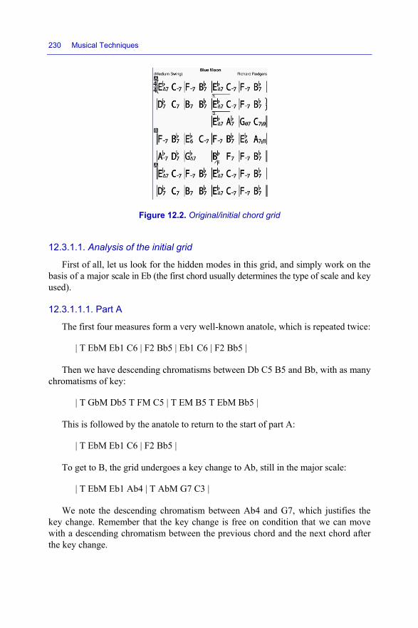
230 Musical Techniques
Figure 12.2. Original/initial chord grid
12.3.1.1. Analysis of the initial grid
First of all, let us look for the hidden modes in this grid, and simply work on the basis of a major scale in Eb (the first chord usually determines the type of scale and key used).
12.3.1.1.1. Part A
The first four measures form a very well-known anatole, which is repeated twice:
| T EbM Eb1 C6 | F2 Bb5 | Eb1 C6 | F2 Bb5 |
Then we have descending chromatisms between Db C5 B5 and Bb, with as many chromatisms of key:
| T GbM Db5 T FM C5 | T EM B5 T EbM Bb5 |
This is followed by the anatole to return to the start of part A:
| T EbM Eb1 C6 | F2 Bb5 |
To get to B, the grid undergoes a key change to Ab, still in the major scale:
| T EbM Eb1 Ab4 | T AbM G7 C3 |
We note the descending chromatism between Ab4 and G7, which justifies the key change. Remember that the key change is free on condition that we can move with a descending chromatism between the previous chord and the next chord after the key change.

Examples of Harmonizations and Compositions 231
12.3.1.1.2. Part B
Part B returns to the scale major of Eb and repeats the anatole, taking the 6th degree away from it, and prepares the ground for a key change to Gb, in the major scale, moving through an A7 11#, which is a Lydian (4th degree) of the major scale of E:
| T EbM F2 Bb5 | Eb1 C6 | F2 Bb5 | Eb1 T EM A4 |
We can see that the key change (we have moved from AbM to EbM) is not made with a descending chromatism. In fact, the C3 at the end of part A is identical to the 6th degree of the scale in Eb, and thus we obtain (C6) F2 Bb5 Eb1, which is the anatole.
We then play an anatole series truncated on a major scale of Gb:
| T GbM Ab2 Db5 | Gb1 |
Again, the key change is justified by the descending chromatism from A4 on a major scale of EM to an Ab2 on a major scale of Gb.
The last two measures of part B lay the foundations for the return to the major scale of A: EbM, by a descending chromatism:
| T FM Bb4 F1 | T EbM F2 Bb5 |
The chromatism involves the chord F which, when we change key, switches from a major chord toa minor chord (descending chromatism of the third))This progression works, above all, because the progression of the last measure is again an anatole on Eb.
We then repeat part A, which we saw earlier.
12.3.1.2. Reharmonization of the initial grid
Now that we have broken the grid down into anatoles and various key changes, we can try to reharmonize the arrangement using different progressions, but which respect the points of transition of the grid.
The key points of the grid are the chords between the anatoles or the key changes to move from part A to B and then from B to A.

232 Musical Techniques
12.3.1.2.1. Part A
| T EbM Eb1 % | % % | Eb1 % | % % |
| T GbM Db5 % | % % |
| T EbM Eb1| ...|
12.3.1.2.2. Switch to B
| T EbM Eb1 % | T AbM G7 % |
12.3.1.2.3. Part B
Part B is a variant of the fundamental anatole, using another key. Let us keep that variant for our transition chords:
– followed by the chord Eb1:
| T EbM Eb1 % | % % | Eb1 T EM A4 |
– followed by:
| T GbM Gb1 % | % % |T FM F1 % | T EbM F2 % |
– and we come back to A:
| T EbM Eb1 % | % % | % % | % % |
Finally, we obtain the following simplified grid:
Figure 12.3. Intermediary chord grid

Examples of Harmonizations and Compositions 233
12.3.1.3. Filling of the final grid
This is the final part of the work of harmonization.
Note that this task is long and painstaking, but it is helpful to explain it here, step by step.
Based on progressions created by descending chromatisms, we can fill the simplified grid found with chords.
12.3.1.3.1. Part A
| T EbM Eb1 % | % % | Eb1 % | % % |
| Db7 % | ….
Let us keep the two series of chords: four chords for the first two measures, and four more for the next two. In the original grid, these two series are identical, but there is nothing to stop us changing series if it sounds good.
1) Start by looking through the long list of progressions (extract below) to find which possibilities might exist, in a scale of EbM (notes: Eb F G Ab Bb C D), which begin with a chord Eb1 [ Eb Bb G D ] and also finish with an Eb1 chord [ Eb Bb G D ]:
100 5 T EbM Eb1 Ab4 D7 Bb5 Eb1 82 5 T EbM Eb1 Ab4 D7 G3 Eb1 80 5 T EbM Eb1 C6 F2 Bb5 Eb1 78 5 T EbM Eb1 Ab4 F2 Bb5 Eb1 52 6 T EbM Eb1 T BbM A7 T EbM Ab4 D7 Bb5 Eb1 51 6 T EbM Eb1 C6 Ab4 D7 Bb5 Eb1 ….
In this list, in the third position, we find the anatole, which was predictable, but there are also other candidates for a harmony – particularly the first progression Eb1 Ab4 D7 Bb5 Eb1 or the second Eb1 Ab4 D7 G3 Eb1. The use of D7 (a semi-diminished) gives the series a particular hallmark.
2) For the next two measures of part A, we move from an Eb1 chord in the scale of EbM to a Db5 chord in the scale of GbM.
Here we go again: we again look in the lists on the basis of the scale in the key of EbM (notes Eb F G Ab Bb C D), for progressions whose chromatisms from a chord Eb1 [ Eb Bb G D ] can lead to a Db5 chord: [ Db Ab F B ] in a scale of the key of GbM (notes: Gb Ab Bb B Db Eb F).

234 Musical Techniques
100 4 T EbM Eb1 C6 T DbM F3 T GbM Db5 60 5 T EbM Eb1 C6 T DbM F3 Db1 T GbM Db5 40 5 T EbM Eb1 T BbM A7 T EbM Ab4 T DbM F3 T GbM Db5 20 10 T EbM Eb1 T AbM Ab1 Db4 Bb2 G7 Eb5 C3 F6 Db4 T GbM Db5 20 16 T EbM Eb1 T AbM Eb5 T EbM Ab4 D7 G3 Eb1 T BbM A7 T EbM Ab4 T DbM F3 T GbM Bb3 Gb1 T BM Gb5 T GbM Eb6 T DbM Ab5 T GbM Ab2 Db5 …………………………………….. 20 6 T EbM Eb1 T AbM Eb5 C3 F6 Db4 T GbM Db5 20 7 T EbM Eb1 T AbM Eb5 T EbM C6 T DbM Ab5 F3 Db1 T GbM Db5 20 9 T EbM Eb1 Ab4 T AbM F6 T GbM Bb3 T AbM Eb5 T GbM Eb6 Ab2 F7 Db5 …
This time, the progressions are more complex because of the key change, but overall we can take the first one which was put forward: a T EbM Eb1 C6 T DbM F3 T GbM Db5. In fact, this choice to move to Db5 using four chords renders the series too complex and cumbersome.
3) It is therefore preferable to make the transition in two steps:
a) to return to an Eb1 in EbM and thus use the progressions from 1);
b) to then vary the next series Eb1 in EbM to Db5 in DbM.
We strictly return to the list from 1):
100 5 T EbM Eb1 Ab4 D7 Bb5 Eb1 82 5 T EbM Eb1 Ab4 D7 G3 Eb1 80 5 T EbM Eb1 C6 F2 Bb5 Eb1 78 5 T EbM Eb1 Ab4 F2 Bb5 Eb1 …..
Let us take the first line Eb1 Ab4 D7 Bb5 and now look for a passage between Bb5 [ Bb F D Ab ] in a key of EbM (scale: Eb F G Ab Bb C D) and Db5 [ Db Ab F B ] in a key of GbM (scale: Gb Ab Bb B Db Eb F).
Yet again, here we go! And again, we look at the possible progressions from EbM to Db5:
100 5 T EbM Bb5 Eb1 Ab4 T DbM F3 T GbM Db5 50 10 T EbM Bb5 G3 Eb1 Ab4 D7 Bb5 G3 C6 T AbM F6 T GbM Db5 50 11 T EbM Bb5 G3 T AbM Eb5 T EbM C6 T AbM Ab1 Db4 T GbM Bb3 T BM Gb5 T GbM Eb6 Ab2 Db5 50 17 T EbM Bb5 G3 T FM C5 T EbM C6 T DbM F3 T EbM D7 T DbM Db1 Gb4 Eb2 Ab5 F3 T GbM Bb3 Eb6 B4 T EM B5 T GbM F7 Db5 …….

Examples of Harmonizations and Compositions 235
Let us take the first series and remove the “useless” chords, because they fall outside of a direct descending chromatism:
100 5 T EbM Bb5 Ab4 T GbM Db5
Thus, we add an Ab4 chord before the move to Db5, which will delay it by a half measure.
Now we need to find a series between Db5 [ Db Ab F B ] in the key of GbM (scale: Gb Ab Bb B Db Eb F) and Eb1 [ Eb Bb G D ] in the key of EbM (scale: Eb F G Ab Bb C D) in only four chords (counting both the beginning and end chords). For this, we re-re-re-read the list of progressions:
100 6 T GbM Db5 T DbM Gb4 C7 T EbM F2 Bb5 Eb1 50 10 T GbM Db5 Bb3 T AbM Eb5 T DbM Eb2 Ab5 T EbM F2 T GbM F7 T EbM Bb5 G3 Eb1 50 13 T GbM Db5 T AbM Bb2 Eb5 T BbM A7 T AbM Ab1 Db4 G7 T EbM C6 F2 T GbM F7 T EbM Bb5 G3 Eb1 50 14 T GbM Db5 Gb1 Eb6 T DbM Ab5 T GbM Ab2 F7 T DbM Bb6 Eb2 C7 T EbM F2 T GbM F7 T EbM Bb5 G3 Eb1 ………..
Take the first series and remove the “useless” chords. It is always useful to play the series in order to extract the chords which are ultimately useful:
100 6 T GbM Db5 T DbM Gb4 C7 T EbM F2 Bb5 Eb1
We retain Db5 C7 Bb5 Eb1, which is a chromatism similar to the original one.
We now seek the passage between Eb1 and F2:
on the basis of the scale EbM: Eb F G Ab Bb C D we look for chromatisms from Eb: [ Eb Bb G D ] which is an
Eb1 to on the basis of the scale EbM: Eb F G Ab Bb C D
F: [ F C Ab Eb ] which is an F2

236 Musical Techniques
Nth consultation of the progression file:
100 3 T EbM Eb1 Ab4 F2 97 3 T EbM Eb1 C6 F2 52 4 T EbM Eb1 C6 Ab4 F2 49 4 T EbM Eb1 C6 T BbM F5 T EbM F2 48 4 T EbM Eb1 T AbM Eb5 T EbM Ab4 F2 48 4 T EbM Eb1 T BbM A7 T EbM Ab4 F2 47 4 T EbM Eb1 C6 T DbM Ab5 T EbM F2 32 4 T EbM Eb1 Ab4 T DbM Ab5 T EbM F2 …………………………………………. 16 5 T EbM Eb1 T AbM Eb5 T EbM C6 T BbM F5 T EbM F2 16 5 T EbM Eb1 T AbM Eb5 T EbM Ab4 T DbM Ab5 T EbM F2 15 5 T EbM Eb1 T BbM A7 T EbM Ab4 T DbM Ab5 T EbM F2
A simple passage to Ab4 will suffice for the transition or a more heavily colored C6.
12.3.1.3.2. Part B
Let us look for something to replace four F2 chords with, ending with an F2.
on the basis of the scale EbM: Eb F G Ab Bb C D we look for chromatisms from F: [ F C Ab Eb ] which is an
F2 to on the basis of the scale EbM: Eb F G Ab Bb C D
F: [ F C Ab Eb ] which is an F2
Reading of the progressions:
100 5 T EbM F2 Bb5 Eb1 Ab4 F2 97 5 T EbM F2 Bb5 Eb1 C6 F2 88 5 T EbM F2 Bb5 G3 C6 F2 83 5 T EbM F2 D7 G3 C6 F2 63 6 T EbM F2 D7 Bb5 Eb1 C6 F2 62 6 T EbM F2 D7 Bb5 Eb1 Ab4 F2 54 6 T EbM F2 D7 Bb5 G3 C6 F2 ……………… 46 6 T EbM F2 Bb5 G3 Eb1 C6 F2 ….

Examples of Harmonizations and Compositions 237
The classic (though truncated) anatole comes in first position, which is perfectly normal but also very predictable harmonically: we can do better! Let us take the second series, enriched with a C6:
F2 Bb5 Eb1 C6 F2
This is followed by four F2 chords which lead to the second part of B and to an Ab2 chord and a key change to GbM.
Let us look for how to move from F2 in EbM to Abm7 in GbM:
on the basis of the scale EbM: Eb F G Ab Bb C D we look for chromatisms from F: [ F C Ab Eb ] which is an
F2 to on the basis of the scale GbM: Gb Ab Bb B Db Eb F
Ab: [ Ab Eb B Gb ] which is an Ab2
Reading of the progressions:
100 9 T EbM F2 D7 G3 T AbM C3 T BbM F5 T AbM F6 T GbM Bb3 Eb6 Ab2
This time, it is more complicated! The key change is difficult, and we only need three chords to fill the grid: thus, let us only take certain chords.
The method to choose which chords will be kept is simple: one chord out of every two, because the ear is capable of constructing the intermediary chord by the descending chromatisms proposed:
F2 G3 F5 Bb3 Ab2
This sounds a little strange, because F2 becomes F5 in the space of a single measure. Let us instead take a progression from F2 to F2, and therefore copy the series used for the previous two measures:
F2 Bb5 Eb1 C6 F2
We follow this with a somewhat brusque chromatism to Ab2 through an Eb6, which is the chord just before Ab2 in the complete series chosen earlier to make the move from F2 in EbM to Abm7 in GbM.
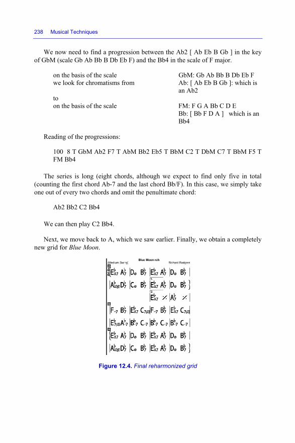
238 Musical Techniques
We now need to find a progression between the Ab2 [ Ab Eb B Gb ] in the key of GbM (scale Gb Ab Bb B Db Eb F) and the Bb4 in the scale of F major.
on the basis of the scale GbM: Gb Ab Bb B Db Eb F we look for chromatisms from Ab: [ Ab Eb B Gb ]: which is
an Ab2 to on the basis of the scale FM: F G A Bb C D E
Bb: [ Bb F D A ] which is an Bb4
Reading of the progressions:
100 8 T GbM Ab2 F7 T AbM Bb2 Eb5 T BbM C2 T DbM C7 T BbM F5 T FM Bb4
The series is long (eight chords, although we expect to find only five in total (counting the first chord Ab-7 and the last chord Bb/F). In this case, we simply take one out of every two chords and omit the penultimate chord:
Ab2 Bb2 C2 Bb4
We can then play C2 Bb4.
Next, we move back to A, which we saw earlier. Finally, we obtain a completely new grid for Blue Moon.
Figure 12.4. Final reharmonized grid

Examples of Harmonizations and Compositions 239
12.3.2. Summertime (by G. Gershwin)
Let us try out the same approach on another jazz masterpiece: George Gershwin’s Summertime.
Figure 12.5. Original/initial arrangement of Summertime
Figure 12.6. Initial grid associated with this arrangement

240 Musical Techniques
12.3.2.1. Analysis of the initial grid
We have one flat in the key, so we are in F major or D minor natural. The first chord often gives the key of the piece of music, and here we are in D-, for the basic key. Note that this is the natural minor scale which corresponds to the Aeolian mode of F. We can work on the basis either of the scale of F major, or of its equivalent in D-7. This point is important, because the minor harmonic scale contains no diminished seventh, unlike with the Aeolian mode.
Let us quickly analyze this very well-known grid and see what we can do with it (whilst remaining very respectful of this composition; we merely want to find different progressions to give a touch of “youth” to this grid, whilst retaining the central chords at the start of each cycle):
– the first chord D-7 is that of the key, which is a D6 of the F major scale;
– the next chord after 4 measures with constant harmony is a G-7, which corresponds to a Dorian of an F major scale or D minor scale;
– the next chord is a Bb7, which, in the scale of F, is a very classic Bb4, followed by an A7, which is an A3 on F (up to this point, the key is constant!);
– we return to D-7, which is the marker of the key, and then go to an FM (F1 in the major scale).
Overall, therefore, we have an arrangement with constant harmony – i.e. based on the same key of the scale throughout the whole of the grid. In fact, all told, it is a fairly simple grid!
12.3.2.2. Harmonization
Let us now move on to the new grid, based on the existing structure so as to preserve the general shape of the arrangement.
D6 to G2 in the major scale of F or D minor:
on the basis of the scale FM: F G A Bb C D E we look for chromatisms from D: [ D A F C ] which is a D6 to on the basis of the scale FM: F G A Bb C D E
G: [ G D Bb F ] which is a G2

Examples of Harmonizations and Compositions 241
Reading of the progressions:
100 2 T FM D6 G2 66 3 T FM D6 Bb4 G2 48 3 T FM D6 T CM G5 T FM G2 48 3 T FM D6 T EbM Bb5 T FM G2 22 4 T FM D6 Bb4 T EbM Bb5 T FM G2 21 4 T FM D6 T CM B7 T FM Bb4 G2
There are multiple choices, and we look for three chords to replace the four D- chords thereafter.
We already know that we can go directly from D6 to G2, because there is a descending chromatism between those two chords. On the other hand, it would be good to enrich the grid somewhat. Let us add a chord at measure 3, and the second series gives us a Bb4 as an intermediary chord.
Thus, we have:
| D6 % | Bb4 % | G2
The G2 is followed by two chords which we keep as they are (we respect what is already in place). We then have a harmonic “hole” (repeating chords) between A3 and D6.
Let us look for a progression between these two chords:
on the basis of the scale FM: F G A Bb C D E we look for chromatisms from A: [ A E C G ] which is an A3 to FM: F G A Bb C D E on the basis of the scale D: [ D A F C ] which is a D6
Reading of the progressions:
100 2 T FM A3 D6 65 3 T FM A3 F1 D6 48 3 T FM A3 T GM D5 T FM D6 47 3 T FM A3 T BbM F5 T FM D6 22 4 T FM A3 F1 T BbM F5 T FM D6 21 4 T FM A3 T GM Gb7 T FM F1 D6

242 Musical Techniques
The passage through an intermediary F (second series here) therefore works here.
Thus, we have: | A3 | F1 | D6 |. However, the grid sounds better if we repeat the A3 rather than add an F1.
The second part of the grid, D-7 (D6) to FM (F1), also needs enrichment:
on the basis of the scale FM: F G A Bb C D E we look for chromatisms from D: [ D A F C ] which is a D6 to FM: F G A Bb C D E on the basis of the scale F: [ F C A E ] which is an F1
Reading of the progressions:
100 4 T FM D6 G2 C5 F1 69 5 T FM D6 Bb4 E7 C5 F1 63 5 T FM D6 G2 E7 C5 F1 52 5 T FM D6 Bb4 E7 A3 F1 51 5 T FM D6 Bb4 G2 C5 F1 51 5 T FM D6 T EbM Bb5 T FM G2 C5 F1 …………… 32 6 T FM D6 Bb4 G2 E7 C5 F1 31 5 T FM D6 G2 C5 T GM Gb7 T FM F1 ….
Here, we are spoilt for choice. In first place, we have the anatole D6 G2 C5 F1, which is an easy solution.
However, as the F1 is placed at the fourth measure after the D6, we shift that of the next measure (the FM), which is replaced by the next chord (D6).
12.3.2.3. Final grid
We obtain a grid that is slightly reharmonized: we have retained the general structure of the initial grid, but it is always possible to start with an even sparser grid (by removing certain interim chords), at the risk of moving substantially away from the original grid.

Examples of Harmonizations and Compositions 243
Figure 12.7. Final reharmonized grid
12.3.3. Sweet Georgia Brown (by Bernie, Pinkard and Casey)
Let us now conclude the presentation of our examples of harmonization with a typical blues arrangement.
Figure 12.8. Original/initial arrangement

244 Musical Techniques
From this arrangement, we extract the following grid.
Figure 12.9. Original/initial grid of chords
12.3.3.1. Analysis of the initial grid
This grid poses a problem because the arrangement having only a single flat in the key is either in F major or in D minor. However, the grid of the arrangement begins in D major! Thus, we are in contradiction with the usual key of an arrangement:
– in this initial grid, we can see that the chords D, G and C are 7th chords, whereas in a conventional scale, only the degrees 3, 4 and 5 are de 7th chords;
– a second “inconsistency” in this grid. The only point which is consistent with the classic major scales is the FΔ at measure 13, which refers to the official key of the arrangement (an F major linked to the only flat in the key).
The only way of analyzing this very strange grid, which begins with a harmonic inconsistency (D7 instead of Dm7), is to use a scale other than the natural major or minor.
Here, we are dealing with a blues scale of the type: C D Eb F Gb G Bb.
This is a fuller scale than the traditional scale, owing to the presence of the D which is usually omitted. It allows for the construction of chords using the same approach as for a major scale.
Let us quickly recap the structure of the chords on the different degrees of a blues scale.

Examples of Harmonizations and Compositions 245
Degrees of the mode
Structure of the chord
Structure of the chordexpressed in C
1 C Eb Gb Bb [ C Eb Gb Bb ] Cm7 5-
2 D F G C [ C Eb F Bb ] Cm…
3 Eb Gb Bb D [ C Eb G B ] Cm M7
4 F G C Eb [ C D G Bb ] C7 sus2 5 Gb Bb D F [ C E Ab B ] CM7 #5
6 G C Eb Gb [ C F Ab B ] CM7 sus4 #5
7 Bb D F G [ C E G A ] C6
Table 12.1. Reminder of the structure of the chords in a blues scale
Thus, there are two degrees with a major chord and a seventh: 4 and 7.
A D7 is therefore that which forms a D4 (the 4th degree in D) on the scale of the key of A, which forms a D7 (the 7th degree in D) on the scale of the key of E.
After the G7, we change key to D now (and the G becomes a G4), followed by a C7.
Finally, we come to the key of F (the official key of the piece), more conventional at measures 1, 3 following by a truncated anatole (2 5 1) and a classic progression also a 6 3 (E7 A3).
12.3.3.2. Reharmonization
We shall leave part 2 as it is, and work on the first 12 measures.
Let us look for a progression on the blues scale from D4 in AB to G7 in AB:
on the basis of the scale blues AB: A B C D Eb E G we look for chromatisms from D: [ D A E C ] which is a D4 to on the basis of the scale blues AB: A B C D Eb E G G: [ G D B E ] which is a G7
Reading of the progressions:
100 2 T AB D4 G7 58 3 T AB D4 B2 G7

246 Musical Techniques
There are few solutions, except to add a B2 (B-7) at measure 3.
Now, we need to move from G7 in AB to C7 in DB:
on the basis of the blues scale AB: A B C D Eb E G we look for chromatisms from G: [ G D B E ] which is a G7
to DB: D E F G Ab A C on the basis of the scale blues C: [ C G E A ] which is a C7
Reading of the progressions:
100 3 T AB G7 T DB E2 C7 33 4 T AB G7 T EB E1 T DB E2 C7
Once again, we can add an E2 from the first series.
We move from the blues scale in D to the major scale in F, and seek the progression between C5 and F1:
on the basis of the scale FM: F G A Bb C D E we look for chromatisms from C: [ C G E Bb ] which is a C5
to FM: F G A Bb C D E on the basis of the scale F: [ F C A E ] which is an F1
Reading of the progressions:
100 2 T FM C5 F1 58 3 T FM C5 A3 F1 32 3 T FM C5 T GM Gb7 T FM F1 18 4 T FM C5 A3 T GM Gb7 T FM F1
The addition of an A3 (second series) is to be expected for measure 11 before the classic passage of the grid.
Note that here, it was possible to preserve classic major scales by using the same key changes, but the example was chosen to highlight the blues scale and its particular qualities.

Examples of Harmonizations and Compositions 247
12.3.3.3. Final grid
Ultimately, we obtain:
Figure 12.10. Final reharmonized grid
12.4. Example of harmonization
12.4.1. Madagascar (by Serge Sibony)
This is a harmonic tapestry of composition on the basis of a simple grid for a bossa-nova rhythm. No – this is no mistake: we have presented no arrangement to this example, because the harmonic content described below invites readers to create/improvise various melodies. Welcome to the world of improvisation!
Let us start with a minimalist grid, which merely outlines the composition:
Figure 12.11. Initial minimalist grid
This minimalist bossa-nova in C major (or A minor) runs through a long series of identical chords at F4. This is nothing inspiring, so we need to enrich this grid.

248 Musical Techniques
We move from a D2 in C to an F4 in C:
on the basis of the scale CM: C D E F G A B we look for chromatisms from D: [ D A F C ] which is a D2 to on the basis of the scale CM: C D E F G A B F: [ F C A E ] which is an F4
Reading of the progressions:
100 4 T CM D2 G5 C1 F4 60 5 T CM D2 B7 G5 C1 F4 51 5 T CM D2 G5 C1 T FM C5 T CM F4 49 5 T CM D2 G5 C1 A6 F4 46 5 T CM D2 B7 E3 C1 F4 46 5 T CM D2 B7 E3 A6 F4 46 5 T CM D2 G5 C1 T GM Gb7 T CM F4 45 5 T CM D2 G5 E3 C1 F4
…. As we need to add three chords between D2 and F4, we more specifically seek
out series of five chords (three new ones plus those already present). Let us take one (the fourth) which sounds good:
D2 G5 C1 A6 F4
This naturally leads us to F7 (#4)
and then between F4 and D2:
on the basis of the scale CM: C D E F G A B search for chromatisms from F: [ F C A E ] which is an F4 to on the basis of the scale CM: C D E F G A B D: [ D A F C ] which is a D2
Reading of the progressions (opening of 19,639 progressions in the file runmaj.txt):
100 2 T CM F4 D2 32 3 T CM F4 T BbM F5 T CM D2

Examples of Harmonizations and Compositions 249
The choice is more limited, and involves a key change. Let us break this series down into two parts:
– the first between F4 and F4 (four measures);
– the second between F4 and D2 (four measures).
In CM from F4 to F4:
on the basis of the scale CM: C D E F G A B we look for chromatisms from F: [ F C A E ] which is an F4 to on the basis of the scale CM: C D E F G A B F: [ F C A E ] which is an F4
Reading of the progressions:
100 5 T CM F4 B7 G5 C1 F4 79 5 T CM F4 D2 G5 C1 F4 79 5 T CM F4 B7 E3 C1 F4 75 5 T CM F4 B7 E3 A6 F4 57 6 T CM F4 B7 G5 C1 A6 F4 51 6 T CM F4 B7 G5 E3 C1 F4 50 6 T CM F4 D2 B7 G5 C1 F4 49 6 T CM F4 B7 G5 E3 A6 F4 49 6 T CM F4 B7 G5 C1 T GM Gb7 T CM F4 47 6 T CM F4 B7 G5 C1 T FM C5 T CM F4 41 6 T CM F4 D2 G5 C1 A6 F4 ….
We have a multitude of choices available. Let us take a series with a high harmony score (the fourth, for example):
F4 B7 E3 A6 F4
The move from F4 to D2 is trickier, because in order to harmonious, the rule of descending chromatism must also be applicable in this progression. Unfortunately, as pointed out in the previous chapter, because we have deliberately limited our calculations of progressions to series of 14 chords at most, in the whole range of possible lists, we find no available progression! Thus, we are witnessing the case of an “irreducible” progression, as discussed in the previous chapter! Therefore, it is necessary to decompose the passage from F4 to D2 via a transitional chord. With this goal in mind, we choose an E-7 which perfectly serves this purpose, because it appears in the previous progression.

250 Musical Techniques
In CM from F4 to E3:
on the basis of the scale CM: C D E F G A B we look for chromatisms from F: [ F C A E ] which is an F4 to on the basis of the scale CM: C D E F G A B
E: [ E B G D ] which is an E3
Reading of the progressions:
100 3 T CM F4 B7 E3 61 4 T CM F4 B7 G5 E3 49 4 T CM F4 D2 G5 E3 49 4 T CM F4 D2 B7 E3 33 4 T CM F4 B7 T AM E5 T CM E3 32 4 T CM F4 T BbM F5 T CM B7 E3 30 5 T CM F4 D2 B7 G5 E3 20 5 T CM F4 T BbM F5 T CM B7 G5 E3 17 5 T CM F4 D2 B7 T AM E5 T CM E3 ….
A transition through B7 is indicated here (first series).
Followed by D2:
on the basis of the scale CM: C D E F G A B we look for chromatisms from E: [ E B G D ] which is an
E3 to on the basis of the scale CM: C D E F G A B D: [ D A F C ] which is a D2
Reading of the progressions:
100 3 T CM E3 A6 D2 53 4 T CM E3 C1 F4 D2 52 4 T CM E3 C1 A6 D2 52 4 T CM E3 A6 F4 D2 49 4 T CM E3 A6 T BbM F5 T CM D2 49 4 T CM E3 T DM A5 T CM A6 D2 …………… 17 5 T CM E3 A6 T GM Gb7 T CM F4 D2 17 5 T CM E3 T DM Db7 T CM C1 A6 D2 16 5 T CM E3 C1 F4 T BbM F5 T CM D2

Examples of Harmonizations and Compositions 251
An A6 fits in well with the progression (first series).
We again find the progression from the four previous measures.
Then we have a D2 to a D2 at the start of the grid:
In CM from D2 to D2:
on the basis of the scale CM: C D E F G A B we look for chromatisms from Dm7: [ D A F C ] which is a D2 to on the basis of the scale CM: C D E F G A B Dm7: [ D A F C ] which is a D2
Reading of the progressions:
100 5 T CM D2 G5 C1 F4 D2 97 5 T CM D2 G5 C1 A6 D2 88 5 T CM D2 G5 E3 A6 D2 83 5 T CM D2 B7 E3 A6 D2 63 6 T CM D2 B7 G5 C1 A6 D2 62 6 T CM D2 B7 G5 C1 F4 D2 ………….. 47 6 T CM D2 B7 E3 C1 A6 D2 47 6 T CM D2 G5 E3 A6 F4 D2 …
Once again, we are spoilt for choice.
The second series repeats the progressions already constructed: D2 G5 C1 A6 D2.
12.4.1.1. Final grid
Finally, we obtain:
Figure 12.12. Final harmonized grid

252 Musical Techniques
However, it is also possible to carry out more complex progressions with key changes (why not?), and obtain:
Figure 12.13. Another solution!
It is true, though, that we are pushing the boat out a little too far with this (re)harmonization.
12.5. Conclusion
We have now come to the end of this final chapter, where we set out to explain in concrete terms, in detail, how to use the harmonic principles set out in theprevious chapters (10, 11, 12) based on the ordering of the thirds, fifths, sevenths, ninths, etc., which are in fact merely clever musical names that are given to the physical harmonic frequencies f, 3f, 5f, 7f, 9f, etc., of course not forgetting the octaves 2f, 4f, etc. (Chapters 4 and 5), and whose mechanical resonances give pleasure to our whole auditory apparatus (Chapter 1).
Conclusion
We have now come to the end of this book, the purpose of which was to give you a sort of “passport” so you can take up and understand specialized works on harmony which are much fuller and of a much higher level than this one. Our main aim was to bring your knowledge up to a level where you are permanently aware of the correspondences between human physiology (the way in which the ear works, etc.), physics (acoustics, spectral analysis, etc.), the mathematical aspects (gentle little reminders), history, civilizations, personal education and technologies (instruments, effects, etc.)… and of course, the majority of musical theories.
If you have any questions, comments, remarks (constructive ones, of course!), you can contact the authors at the addresses shown below. You will always be more than welcome to do so: this kind of contact can only enrich everybody’s knowledge!
DOMINIQUE PARET: [email protected]
SERGE SIBONY: [email protected]
Musical Techniques: Frequencies and Harmony, First Edition. Dominique Paret and Serge Sibony. © ISTE Ltd 2017. Published by ISTE Ltd and John Wiley & Sons, Inc.

Appendix
Acoustic (Harmonious) Effects
Although they are not pure harmony, per se, acoustic effects have a significant influence on whether or not the overall sound is pleasant, whether it is harmonious or not, and so they do contribute to what we know as harmony. We believe that this little aside is, in fact, within the bounds of the subject, and present this appendix on the numerous classic effects which are frequently employed so that music sounds even better!
Acoustic effects are merely physical effects of various types of modulations of the basic functions mentioned above, the intrinsic frequencies of the notes, their amplitudes, their relative phases, the instantaneous or longer-lasting modification of the contents of their harmonic spectra, also help to fill out the volume of the piece.
A.1. Stereophonic effect
Let us skip over the trivial monophonic effect, and briefly examine the phenomenon that occurs in the presence of two or more sound sources physically present in the same spatial volume.
The average distance between an individual’s two auditory systems is around 8-12.5 cm. Those of you who think you have a large head and who may think this sounds too little, do not be tempted to try and measure this distance. It is the distance between the two eardrums. Now you have been reassured, let us look at a few simple calculations.
We know that sound propagates in air at around 340 meters per second, and that therefore, a sinusoidal sound wave (e.g. somebody whistling) coming from a source which is at an unequal distance from the two eardrums will not reach both eardrums at exactly the same time (in reality, there will be a certain phase shift). For this
Musical Techniques: Frequencies and Harmony, First Edition. Dominique Paret and Serge Sibony. © ISTE Ltd 2017. Published by ISTE Ltd and John Wiley & Sons, Inc.
256 Musical Techniques
reason, we have the feeling of left and right sounds, and thus the effect of a stereophonic, 3D soundscape.
We can calculate the value of the frequency “F” for which that the phase shift due to a time lag between the arrival at the two eardrums is maximal – i.e. the frequency at which the stereophonic effect is most marked. The maximum effect, of course, corresponds to the time at which the two signals reaching the eardrums have the greatest phase difference – i.e. when they are in phase opposition.
If the wavelength of the frequency F in question is λ (lambda), the aforementioned maximum will take place at the time when λ/2 is equal to the distance between the eardrums. However, there is a direct relation between λ and the celerity of sound propagation “v”, and the period T = 1/F of the signal:
λ = v × T = v × (1/F)
If the distance between the eardrums = λ/2 = 0.125 m, i.e. λ = 0.25 m:
then F = 340/0.25
= 340 × 4 = 1360 Hz
= around 440 Hz × 3
= which is around one octave and a (perfect) fifth above la3, which is mi5
Let us state, then, that in the band around 1-2000 Hz, the phase difference between the two ears, through the whole of our auditory system, will produce an effect, an impression of volume and/or position which is more pronounced than with a monophonic sound source.
A.2. Effect of vibrato
Vibrato (taken from the Italian substantive, derived from the adjective vibrato, meaning “vibrated”) is a periodic modulation of the sound of a musical note. The nature of that modulation (whether or not is purely a modulation of pitch) depends on the nature of the instrument and on the technique the musician is used.
In principle, this effect consists only of modulating the frequency F of a note around its central value without modulating its amplitude. By how much? That is a good question. How quickly? Again, a good question.

Appendix 257
Consider the example of the violin. We place a finger on the string and do not move it, and we obtain a normal note – cold-sounding and lifeless. If we want to give it some body, some soul, we very slightly shift the finger (or alter the pressure of the finger) to either side of the initial position, which modifies the frequency emitted… in other words, the height of the note.
On the violin and on bowed strings, this modulation, which is produced by a motion of the finger on the string, relates to the height of the sound, but the intensity, controlled by the bow, is kept constant.
A.2.1. By how much?
The aim here is to modulate (both positively and negatively) the length of the vibrating string, and thus “slightly modulate the frequency” emitted by +/- ΔF, and consequently the pitch of the note.
What amplitude of modulation should be used? How much? This is up to your instinct as a player: a little… or a lot.
A few harmless little savarts (4, 5, etc.), or a quarter tone (12.5 savarts). It is up to you to draw your own inspiration, but be warned: once you modulate the note by as much as a semitone, you are beginning to play a different melody… with a different harmony!
A.2.2. How quickly?
As fast as your finger, wrist or forearm can move! Watch violinists or cellists during a concert! In other words, modulate at a human speed! As an order of magnitude, 2-8 times per second tends to sound pleasant – i.e. generally around 6Hz or slower.
EXAMPLE.– Let us look at the example of the vibrato on the electric guitar (incorrectly referred to by many guitarists as tremolo – see the distinction below) – in this case, a mechanical device (the small vibrato bar or arm on the legendary Fender Stratocaster guitar – see Figure A.1) allows the player to add or release tension, very slightly, simultaneously on all the strings of the instrument.

258 Musical Techniques
Figure A.1. The legendary vibrato/tremolo system on the Fender Stratocaster. For a color version of this figure, please see www.iste.co.uk/paret/musical.zip
NOTE.– The piano and harpsichord are incapable of vibrato, but the clavichord can deliver a vibrato in terms of height, with no intensity modulation, by modulating the pressure of the finger on the key. Finger vibrato, with pitch modulation but no intensity modulation, is used on lutes, guitars and other plucked string instruments. Vibrato, on amplified instruments (e.g. the Hammond organ, the electric guitar, etc.) can also be produced electromechanically (though this must not be confused with the effect of the Leslie cabinet – see below).
Like all nuancing effects, vibrato lends particular expressiveness depending on how it is produced: quickly or slowly, fluidly or spasmodically… etc.
Vibrato was the first effect to be replicated electronically. A device takes the electrical signal produced by the instrument and rapidly varies its frequency. In other words, it varies the height of the sound around its original tone.

Appendix 259
Electronic vibratos perform the same type of modulation as electric guitars. Generally, the modulation takes place on the master oscillator (Figure 2.4) so that all the notes vary by exactly the same percentage (degree of modulation) and at the same rate of modulation.
A.3. “Tremolo” effect
It is important to distinguish “tremolo” from “vibrato”. Tremolo, consists of varying (mainly) the intensity of the note around a mean value whilst largely preserving the initial pitch (see section A.3.1).
In wind instruments, the periodic modulation of amplitude created by the player’s diaphragm pertains more to the intensity of the sound than to its frequential height. In an organ, a mechanical device on the wind pipe, known as the “tremulant”, produces a similar effect (modulation of intensity, mainly).
A.3.1. Example: Leslie cabinet
Very widely used with jazz organs (Hammond organs, for example), the original models of the most typical (old-school) Leslie speakers are made up of a 40-watt (tube) amplifier and two loudspeakers. The sound issuing from the instrument (original acoustic output signal) is separated/dispatched with two second-order frequency filters at 12 dB/octave – a “high-pass” filter and a “low-pass” filter, whose cutoff frequencies are identical (in the original cabinet made by Leslie/Hammond, that value is around 800 Hz, and it is generally from ~600 to 1200 Hz), to send low-pitched sounds to the mid/bass speaker (a woofer) and high-pitched sounds to the treble speaker (known as a tweeter). The membrane of the mid/bass speaker is directed toward the ground, and the sound it produces passes through a light rotating drum, made of polyester, having a specific hollowed-out shape on one part of its circumference. The high-pitch speaker is orientated toward the top of the cabinet, and the sound from the tweeter travels through a rotating double trumpet (horn).
Figures A.2 to A.5 illustrate the mechanics that produce this sound modulation:
– for trebles, the horn rotates at a very fast speed;
– for mids and bass sounds, the speed of rotation of the drum is medium/fast or slow.

260 Mu
FiguFor a
In geable to wrotation mass andtime (a
usical Technique
Figu
ure A.3. View a color version
eneral, the druwork at two rospeeds of thed its inertia, tgood few ten
MotoRapid
Tr
MotoS
Mid/Mi
es
ure A.2. Elect
of the rotor/drn of this figure
um and horns rotation speedse drum are slothe main drum
nths of a seco
r 1 for horns single-speedTreble horn
reble speaker
or 2 for drum Slow 2-speed/bass speakerid/bass drum
trical diagram
rum (mids ande, please see w
rotate in oppos (known as chower than thom has much lond) than thos
of a Leslie cab
d basses) andwww.iste.co.u
osite directionhorale and treose of the horlonger accelerse of the treb
binet
d the horn (trebuk/paret/music
s, and only themolo). In addrns and, becauration and de
ble horns. Thi
bles). cal.zip
he drum is dition, the use of its
eceleration is creates

particulapieces (e
Figuat star
co
Very thidampen
Leslie in
Thus, 25
ar deliberate efxamples: Jimm
ure A.4. Detailrtup and stoppolor version of
Figure A.5integrate
pl
V. lightweigDri
ck wood to vibrations
nside
50–300 kg!
ffects as they my Smith, Boo
led view of hopage are very f this figure, pl
5. Example of ed Leslie spealease see ww
Horn
Drive belt
ght polyester druive belt not visib
are set in mooker T, etc.).
rns and drumsdifferent betwlease see ww
a top-of-the raker. For a colo
ww.iste.co.uk/p
um ble
otion and stopp
s. Please noteween the horn ww.iste.co.uk/p
ange chamberor version of th
paret/musical.z
Appen
ped, particular
e that inertia vand the drum
paret/musical.z
r organ with his figure, zip
ndix 261
rly in jazz
values m. For a zip

262 Musical Techniques
The double rotations mentioned above cause variations:
– the rotation of the hollowed-out area of the polyester drum varies the amplitude of the sound (the sound seems to move closer and further away), which produces a panoramic effect, filling the volume of the room in which we are playing (because in addition, due to the rotation of the inside of the drum, the sound moves from left to right as a function of the rotation);
– consequently, this produces a mechanical modulation of the frequency and the phase of the sound wave, creating a Doppler effect.
REMARK.– With wear and tear, the drive belts of the drums and horns – see Figure A.4 – begin to make a little noise (it is possible to adjust the tensions on these belts, but few people are sufficiently puritanical to do it!)
As it rotates, the lower drum creates a bit of a breeze, which, in summer, is refreshing for the feet if one is playing barefoot!
These last two properties, of course, are rendered obsolete by the creation of purely electronic Leslie effects, but obviously, this is less fun!
A.4. Doppler effect
In 1842, Christian Doppler put forward a description of the effect which, today, bears his name. He confirmed that the pitch of the perceived sound was higher than the emitted frequency as the source approaches the observer, and lower than the emitted frequency as the source moves away.
Briefly, in classic physics, we can show that when the speed of movement of the source and of the receiver are slower than the celerity of the soundwaves in the medium, the relation observed between the frequency f and the emitted frequency f0 is given by:
0⎛ ⎞
= ⎜ ⎟⎝ + ⎠
+ r
sf fυ υ
υ υ
In this equation:
– υ velocity of the waves in the medium;
– rυ velocity of the receiver in relation to the medium – positive if the receiver approaches the source;

Appendix 263
– sυ velocity of the source in relation to the medium – positive if the source moves away from the receiver.
The above formula applies to the soundwave if and only if the velocities of the source and the receiver are slower than the celerity of the sound emitted, and also requires the source of the sound to come closer or move away on the axis in relation to the observer. If the source approaches the observer at a given angle (but still at a constant velocity), the frequency heard is higher than that which is emitted by the object. Thereafter, there is a monotonous increase in the observed frequency as the sound source approaches the observer, until equal pitch when the object is as close to the observer as it can be, followed by a continuing monotonous decrease as the source moves away from the observer. When the observer is very close to the object’s path, the move from high to low frequency is very abrupt, and when s/he is far from the object’s trajectory, s/he experiences more of a gradual shift from high to low frequency.
Within the range where the velocity of the propagated wave is much greater than the relative velocity of the source and observer, the relation between the observed frequency f and the emitted frequency f0 is given by:
Observed frequency Variation in frequency
,01
⎛ ⎞= −⎜ ⎟⎝ ⎠
s rf fc
υ ,
00
,Δ = − =λ
−s r s rf fc
υ υ
where:
– , ,= −s r s rυ υ υ velocity of the source in relation to the receiver, positive when the source and receiver are moving away from one another;
– c , celerity of the wave (e.g. 340 m/s for sound);
– 0λ , wavelength of the wave diffused.
These two equations are accurate only to a first-order approximation. However, they hold true when the velocity between the source and the receiver is relatively low in relation to the celerity of the waves involved, and the distance between the source and receiver is relatively greater than the wavelength.
If either one of these two approximations is not satisfied, the formulae are no longer accurate.

264 Musical Techniques
A.5. Effect of complete or partial detuning: example: a tack piano
In a piano, by introducing a slight gap (detuning), constant but random, of the order of 2-5 Hz – you can count the number of savarts you want for the right amount of harshness and dissonance – in the heights of the frequencies of the 2 or 3 strings in each group for each note, we obtain the “tack piano” sound that is quintessentially 1925, characteristic of the Charleston years, of the accompaniment to silent films in the cinema, of the musical ambiance of the spaces of yesteryear; the atmosphere evoking the saloons of the American Wild West and the honky-tonk of the South, or indeed, applied to ragtime or country airs.
More simply, on a polyphonic synthesizer, take two different channels, each with two identical sounds of pianos whose tuning frequencies are strictly identical. Now, slightly detune each of them (e.g. using the detuning function on a Yamaha synthesizer) to either side of that central frequency. Of course, you lose the exact consonance, and depending on that value of the detuning, determining the harshness of the interval, you obtain a magnificent tack-piano effect. With these experiments completed, just for your own general knowledge, note the values of the tuning frequencies for the two pianos!
NOTE.– Some readers must surely have allowed a smile to creep across their faces as they read the previous paragraph, seeing it as reinventing the wheel, saying that everybody knows this and has done for a long time (pianos existed long before synthesizers did!): how to detune a piano to make it a tack piano, by playing on the relative detuning of each of the strings present (2 or 3) per note, or indeed by stuffing it with newspaper! Of course, they are absolutely right! Nevertheless, to do so takes a great deal of time and patience, and when you have had enough of that clunky, tack sound, you simply need to retune everything to normal, which will take a certain amount of time… On a synthesizer, though, it is much easier: it takes all of two seconds, in both directions. A done deal!
A.6. Chorus effect (often used with strings – violins, etc.)
A good example of the chorus effect is that which is created by an ensemble of strings (violins, etc.) not all playing strictly at the same time (see phasing) and not all precisely tuned to the same frequencies in the range of harshness (thus not dissonant), and whose frequencies and/or phases vary slightly over time.
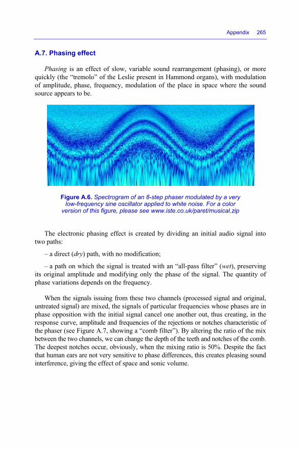
Appendix 265
A.7. Phasing effect
Phasing is an effect of slow, variable sound rearrangement (phasing), or more quickly (the “tremolo” of the Leslie present in Hammond organs), with modulation of amplitude, phase, frequency, modulation of the place in space where the sound source appears to be.
Figure A.6. Spectrogram of an 8-step phaser modulated by a very low-frequency sine oscillator applied to white noise. For a color
version of this figure, please see www.iste.co.uk/paret/musical.zip
The electronic phasing effect is created by dividing an initial audio signal into two paths:
– a direct (dry) path, with no modification;
– a path on which the signal is treated with an “all-pass filter” (wet), preserving its original amplitude and modifying only the phase of the signal. The quantity of phase variations depends on the frequency.
When the signals issuing from these two channels (processed signal and original, untreated signal) are mixed, the signals of particular frequencies whose phases are in phase opposition with the initial signal cancel one another out, thus creating, in the response curve, amplitude and frequencies of the rejections or notches characteristic of the phaser (see Figure A.7, showing a “comb filter”). By altering the ratio of the mix between the two channels, we can change the depth of the teeth and notches of the comb. The deepest notches occur, obviously, when the mixing ratio is 50%. Despite the fact that human ears are not very sensitive to phase differences, this creates pleasing sound interference, giving the effect of space and sonic volume.

266 Musical Techniques
Figure A.7. Response (on a horizontal logarithmic scale) of a comb filter
NOTE.– The definition of a phaser generally excludes devices where the all-pass section is a delay line; a device such as this is called a flanger (see below).
As opposed to “low-pass” or “high-pass” frequency filtering circuits, traditional electronic phasers use a series of “all-pass” networks with varying phase shifts which modify the phases of the different frequency components of the incident signal. These networks thus allow all frequencies to pass through at an equal level, merely introducing phase changes to the signal.
A simplified structural diagram for a mono phaser is indicated below:
Figure A.8. Example of the simplified structure of a mono phaser
The number of all-pass filters (usually called stages) varies with different models. Certain analog phasers offer 4, 6, 8 or 12 stages. A digital phaser may offer up to 32 or even more. This value determines the number of notches in the response curve, which affects the general character of the sound. A phaser with n stages generally has n/2 notches in the spectrum. In addition, the output can be fed back to the input (“feedback”) to create a more intense resonance effect by emphasizing frequencies between notches, as shown in Figures A.10 and A.11.

Appendix 267
Figure A.9. Example of a phaser with feedback
The frequency response of an 8-stage phaser with or without feedback.
Figure A.10. Frequency response of an 8-stage phaser without feedback, dry/wet ratio: 50/50%
Figure A.11. Frequency response of an 8-stage phaser with 50% feedback, dry/wet ratio: 50/50%
NOTE.– Note that the peaks between notches are sharper when there is feedback, which produces a very distinct sound. A stereo phaser is generally built with two identical phasers whose right and left channels are modulated by a quadrature signal (phase-shifted by 90°). Modern phasers have DSPs (digital signal processors) which often aim to imitate analog ones. They generally come in the form of plugins for sound-editing software, as part of a monolithic sound-effect unit, in a “19-inch

268 Musical Techniques
rack”, or indeed in guitar “effects pedals”, and are often used for effects on drums and electric guitars.
A.8. Flanging effect
History tells us that in the spring of 1966, tired of the lengthy process of re-recording to create two vocal tracks, John Lennon of the Beatles asked Ken Townsend, the EMI engineer at Abbey Road Studios, if there was any electronic means of obtaining the sound of the doubled voice without actually doing all the work twice. After analyzing the problem and the tape echo chambers used at the time, the process developed is generally known as Artificial Double Tracking, or ADT, and it was John Lennon who is thought to have given the name flanging to that process.
A.8.1. Flanging original
Flanging is a specific type of phasing.
The effect known as flanging is a complex sound effect which occurs when we mix two identical signals, one of which is delayed (either mechanically or using a delay line) by a very short period of time, generally less than 20 milliseconds, and changing little by little.
In fact, the name flanger comes from the original method of creating the effect and designing a device specifically for the purpose of creating that sound effect.
A.8.1.1. Principle
Originally, the same signal was recorded simultaneously on two tape recorders. The output signals from the play heads of those two recorders were then mixed together on a third machine. Hence, the slightest differences in the recording/playback speeds of the motors for each tape recorder gave rise to a “phasing” effect when the signals were combined. The origin of the effect of flange stems from the fact that in order to amplify this effect of slight, variable phasing, a sound engineer would literally hold his/her finger to the edge of one of the two reels (the flange) so its speed was slowed, to a greater or lesser degree. When the sound engineer removed his finger, the tape would speed up. This effect of slowing and acceleration produced phase shifts desyn-chronized by a few minuscule degrees, and on listening, created variations in sums and differences in harmonics.

Appendix 269
In 1969, Warren Kendrick designed a method to more closely control the flanging effect by having two Ampex stereo tape recorders side by side, running at 15 IPS (15 inches per second – i.e. 38 cm/s).
Figure A.12. Historical setup for the principle of flanging. For a color version of this figure, please see www.iste.co.uk/paret/musical.zip
As indicated by Figure A.13, the receiving reel of recorder A and the feed reel of recorder B were inactive (no load), as were recording channel 2 on recorder A and recording channel 1 on recorder B, as well as the erase head on recorder B.
The tape running between the two recorders is fed from left to right, and an identical signal has been recorded on each channel (1 and 2) of the tape, but shifted by around 18 inches (45 cm) along the length of the tape (which equates to around 1.2s in terms of time). During the recording, skillfully, using a screwdriver (not a magnetic one, of course) inserted between the two recorders, it was possible to force the tape to do a little additional mechanical “rise” and “fall”. The same setup was used for playback/mixing onto a third recorder. The screwdriver, when moved from front to back, causes the two signals to diverge and then converge. This latter technique creates zero-flanging points – i.e. points where the delayed signal crosses the attack signal and the signals change places.
In the same way as phasers, this technique creates an unlimited series of peaks and notches, evenly spaced. The notches thus created by mixing the signal with a delayed portion of itself tend to produce a sound which seems more natural than a phaser does. In addition, it is possible to cascade a delay line with another type of all-pass filter. Thus, it combines the flanger’s unlimited number of notches with the phaser’s irregular spacing, and this produces a comb filter effect that varies over time as a function of the delay times (we call this a swept comb filter effect… which sounds more worthy of a hair salon than a music studio!).

270 Musical Techniques
A portion of the output signal from the flanger is generally fed back into the input (a “recirculation in the delay line”), creating a resonance effect which further enhances the intensity of the peaks and troughs. The phase of the feedback signal is sometimes reversed, causing another variation on the flanging sound. In short, when it comes to fantasies and electronic sound engineering, anything goes!
A.8.1.2. Barber-pole flanging
The barber pole is a well-known sight (Figure A.14). It is the red, white and blue spiral emblem used by barbers (or hairdressers), rotating endlessly, with its lines seeming to go on into infinity.
Barber-pole flanging is also known as “infinite flanging”. The sonic illusion of such flanging is such that the frequency sweeping of the sound seems to move infinitely in one direction, either upwards or downwards, instead of move backwards and forwards on both sides of an initial phase. To create this effect, barber-pole flanging uses a cascade of multiple delay lines. This effect is available on many hardware- and software effects systems.
Figure A.13. The conventional red, white blue spiral emblem for barbers (or hairdressers), known as a barber pole. For a color
version of this figure, please see www.iste.co.uk/paret/musical.zip
A.8.2. Artificial flanging
Nowadays, the flanger effect is created using integrated circuit technology, either in analog or primarily in digital, using DSP technology. Flanging can also be done by software.

Appendix 271
A.8.3. Comparison of the phaser and flanger
In phasing, the signal is transmitted through one or more all-pass filters whose phase response is nonlinear, and then is added to the original signal. This causes both constructive and destructive interference which varies with the frequency, giving a series of peaks and troughs in the system’s frequency response. In general, the position of these peaks and troughs does not occur in a harmonic series. Phasing gives a comb filter with irregularly spaced teeth.
Figure A.14. Spectrograms of phasing effects
In flanging, we add to the signal a partial copy of itself, delayed over time, resulting in an output signal with peaks and troughs which are in a harmonic series. The flanger acts as a comb filter whose teeth are regularly spaced.
Figure A.15. Spectrograms of flanging effects
For both phasing and flanging, the characteristics (respectively the phase responses and the delay effects) vary over time, leading to the effect of sweeping of
Phasing effect
Flanging effect

272 Musical Techniques
the audible spectrum. To the ear, flanging and phasing seem similar, but can be told apart because of their distinct colorations (different spectral contents).
So that the comb filter effect will be perceptible, it is preferable that the spectral content of the sound source be sufficiently complete within the frequency range of the comb filter, variable to reveal the effect of the filter. The richer the harmonic content is in terms of white-noise signals, similarly broad-spectrum noise signals (e.g. Dirac pulse, i.e. percussion, i.e. drums), the better the effect that will be produced!
Glossary
For beginner musicians, here is a brief glossary of the main terms employed in this book (further details given in the various chapters).
Air: a song or melody.
Alteration: the raising or lowering of a note by means of a sharp or flat.
Altered chord: a chord in which a note(s) has been raised or lowered chromatically.
Atonal: music that is written and performed without regard to any specific key. Music that lacks a tonal or key center.
Attack: the beginning of a sound.
Augmented sixth chord: a kind of chord in which the interval of an augmented sixth resolves outward to an octave. Contains an augmented sixth above the bass, in addition to various other tones.
Authentic cadence: a cadence with a progression from the dominant (V) chord to the tonic (I) chord.
Bemolle (or flat): a symbol indicating that the note is to be diminished by one semitone. The symbol that means to lower the pitch one half step (b). Accidentals that lower a given pitch by one half-step.
Cadence: a sequence of chords that brings an end to a phrase, either in the middle or the end of a composition.
Canon: the strictest form of musical imitation, where one part begins, and the other part begins later the exact same line (see ROUND).
Circle of fifths: order in which the successive fifths are arranged.
Musical Techniques: Frequencies and Harmony, First Edition. Dominique Paret and Serge Sibony. © ISTE Ltd 2017. Published by ISTE Ltd and John Wiley & Sons, Inc.
274 Musical Techniques
Choir: a group that sings in unison.
Chord: two or three or more notes played simultaneously in harmony.
Chord progression: a string of chords played in succession.
Chromatic: moving in half-steps.
Chromatic scale: includes all twelve notes of an octave.
Clef: a symbol at the beginning of the staff defining the pitch of the notes found in that particular staff.
Consonance: groups of tones that are harmonious when sounded together as in a chord.
Degree: a note of a scale, identified by number.
Diatonic: moving within a key without changes. The notes indigenous to a key in a major or minor scale.
Diesis (or more usually, sharp [plural: dieses]): a symbol indicating the note is to be raised by one semitone. the symbol that indicates moving one half step higher (#). An accidental that raises a given pitch by one half-step.
Diminished: lowered, or reduced.
Diminished seventh chord: a chord made up of a root, a minor third, a diminished fifth, and a diminished seventh.
Diminished triad: a triad which contains a root, a minor third, and a diminished fifth.
Dissonance: harsh, discordant, and lack of harmony. Also a chord that sounds incomplete until it resolves itself on a harmonious chord. Notes that conflict, or sound outside of a chord in which they occur. Such notes usually fall outside of the overtones which are being generated by the note or chord that is sounding. A combination of two or more tones that create tension and must be “resolved” with standard chords (ones that are expected, or pleasant to the ear).
Dominant: the fifth degree of the diatonic major or minor scale.
Double flat: an accidental that lowers the note it precedes by one whole step.
Double sharp: an accidental that raises the note it precedes by one whole step.
Equal temperament: tuning of an instrument whereby the octave is divided into equal intervals.

Glossary 275
Fourth: the interval of four diatonic degrees. The interval between two notes. Two whole tones and one semitone. make up the distance between the two notes.
Fifth: the interval between two notes. Three whole tones and one semitone make up the distance between the two notes. The interval of five diatonic degrees.
Fundamental (or root): the lowest note in a harmonic series.
Harmonics: series of multiple or fractional sounds existing within a tone produced by the vibration of the parts of the instrument/larynx.
Honky tonk: a country music style known for its powerful, emotional songs.
Interval: the distance between two notes. The distance in pitch between two notes.
Intonation: the manner in which tones are produced with regard to pitch.
Jazz: a genre in which artists improvise within a rhythmic and harmonic framework.
Key of Fa (F): also called the “F” clef); the sign on the staff that indicates pitches. Where the 4th line (up) represents the F below Middle C.
The F clef falling on the fourth line of the staff.
Key of So (G): a clef that indicates which line represents G on a staff, as opposed to a C clef, or an F clef.
Key signature: the flats and sharps at the beginning of each staff line indicating the key of music the piece is to be played.
Major: one of the two modes of the tonal system.
Major chord: a triad composed of a root, a major third, and a fifth.
Major key: based on a scale of w/w/h/w/w/w/h steps.
Major scale: a diatonic scale in which the half steps fall between the third and fourth, and the seventh and eighth degrees.
Measure: the unit of measure where the beats on the lines of the staff are divided up into two, three, four beats to a measure.
Melody: pitches in sequence that form a pattern.
Music element that is a combination of pitches arranged in orders that are usually pleasing to hear. Pitches move up, down, or repeat to make a melody. a tune, or the notes of a song
Minor: one of the two modes of the tonal system. The minor mode can be identified by the dark, melancholic mood.

276 Musical Techniques
Minor key: based on a scale of w/h/w/w/h/w/w steps.
Mode: a type of scale with a specific arrangement of intervals. The modes are either major or minor.
Modulation: to shift to another key.
Natural: a symbol that returns a note to its original pitch after it has been augmented or diminished. The symbol that means to return a pitch to it’s “natural” status.
Ninth: the interval of nine diatonic degrees (an octave and a second).
Octave: the pitch that is exactly 1/2 the number of vibrations or exactly twice the number of vibrations of a starting pitch: Also a series of eight diatonic full tones above the key note where the scale begins and ends.
Pentatonic scale: a musical scale having five notes. For example: the five black keys of a keyboard make up a pentatonic scale.
Pitch of a note (occasionally height): the frequency of a note determining how high or low it sounds.
Reed: the piece of cane in wind instruments. The players cause vibrations by blowing through it in order to produce sound.
Register: a portion of the range of the instrument or voice.
Relative major/minor: the major and minor keys that share the same notes in that key. For example: A minor shares the same note as C major.
Relative pitch: ability to determine the pitch of a note as it relates to the notes that precede and follow it.
Release: how a sound is ended.
Resolution: the progression of chords or notes from the dissonant to the consonant or point of rest.
Resonance: when several strings are tuned to harmonically related pitches, all strings vibrate when only one of the strings is struck.
Rythm: the element of music pertaining to time, played as a grouping of notes into accented and unaccented beats. Combinations of, or patterns of long and short sounds, including a regular phrase.
Scale: successive notes of a key or mode either ascending or descending.
Semitone: the smallest interval. There are 12 half-steps in an octave.

Glossary 277
Seventh: the interval between the first and seventh degrees of the diatonic scale.
Sixth: the interval of six diatonic degrees.
Slide: a glissando or portamento. Also refers to the moving part of a trombone.
Standard: a song that is often recorded and performed.
Temperament: refers to the tuning of an instrument.
Tempo: indicating speed. Speed of the pulse (beat), with terms for fast or slow. The speed at which a regular pulse is repeated.
Tessitura: the range of an instrumental or a vocal part.
Texture: the “thickness” of harmony--how many interwoven parts?
Third: the interval of three diatonic scale degrees.
Timbre/tone color: the relative brightness or darkness of a sound.
Tonality: the tonal characteristics determined by the relationship of the notes to the tone.
Tone: the intonation, pitch, and modulation of a composition expressing the meaning, feeling, or attitude of the music.
Tremolo: quick repetition of the same note or the rapid alternation between two notes.
Triad: three note chords consisting of a root, third, and fifth.
Triton: a chord comprised of three whole tones resulting in an augmented fourth or diminished fifth.
Tuning: the raising and lowering a pitch of an instrument to produce the correct tone of a note.
Unison: two or more voices or instruments playing the same note simultaneously. Everyone on the same pitch.
Vibrato: creating variation pitch in a note by quickly alternating between notes.
Voice: one of two or more parts in polyphonic music. Voice refers to instrumental parts as well as the singing voice.
Whole-tone scale: a scale consisting of only whole-tone notes. Such a scale consists of only 6 notes.

Bibliography
ABROMONT C., Guide de la théorie de la musique, Henry Lemoine, Paris, 2001.
ANGER-WELLER J., Clés pour l’harmonie, Henri Lemoine, Paris, 1990.
BAUDOIN P., Jazz, mode d’emploi, Editions Outre Mesure, Paris, 2004.
BOUDIER A., GUIBERT E., Cours d’acoustique, Techniciens supérieurs son 1re année, 2006–2007.
BRĂILOIU C., ROUGET G., Problèmes d’ethnomusicologie, Minkoff, Geneva, 1973.
CACHET F., “Computer analysis of jazz chorus sequences: is polar a blues ?”, in E. Miranda, Readings in Music and Artificial Intelligence, Harwood Academic Publishers, Reading, 2000.
DANHAUSER A., Théorie de la musique, Henri Lemoine, Paris, 1929.
DELPRAT N., Le Son Musical, Conférence pour L2 University of Paris VI, Paris, 2005–2006.
FRIEDMANN M.J., “A generative grammage for Jazz Chorus”, Music perception, vol. 2, no. 1, pp. 52–77, 1984.
GALLAS P., La musique moderne – volume 4 : tous les accompagnements dans tous les styles, Henri Lemoine, Paris, 1981.
GONIN F., LE TOUZÉ D., Manuel d’analyse harmonique et tonale, De Plein Vent, 2002.
GOYÉ A., La perception auditive, ENST cours P.A.M.U., January 2002.
JULIEN I., CATALDO J.L., Traité de l’arrangement : volume 1, Editions Média Musique, 2005.
LEIPP E., Acoustique et musique, Masson, Paris, 1976.
MATRA J.J., Acoustique et électroacoustique – tome 1, Eyrolles, Paris, 1964.
MERCIER D., Livre des techniques du son – tome 1 : notions fondamentales, Dunod, Paris, 2002.
PACHET F., “Surprising Harmonies”, International Journal on Computing Anticipatory Systems, 1999.
Musical Techniques: Frequencies and Harmony, First Edition. Dominique Paret and Serge Sibony. © ISTE Ltd 2017. Published by ISTE Ltd and John Wiley & Sons, Inc.

280 Musical Techniques
SIBONY S., Enchaînements Harmoniques par les modes – volume 1, EdiLivre, Paris, 2015.
SIBONY S., Listing d’enchaînements harmoniques – gammes blues, available at: www.lulu. com, 2016.
SIBONY S., Listing d’enchaînements harmoniques – gammes majeures, available at: www. lulu.com, 2016.
SIBONY S., Listing d’enchaînements harmoniques – gammes mineures, available at: www. lulu.com, 2016.
SIBONY S., Listing d’enchaînements harmoniques – gammes ton/ton, available at: www. lulu.com, 2016.
SIRON J., La partition intérieure, Editions Outre Mesure, Paris, 1992.
Websites
www.cned.fr (séquence 1 SP03)
www.jeanpierrepoulin.com/Mode.htm

Index
A, C, D
air, 8, 9, 14, 58, 59, 130, 175 alteration, 114, 139, 164, 185, 186 attack, 61 cadence, 196, 198, 207 canon, 151 chord progression, 198, 202, 209, 212 chords
fifth, 31, 33–41, 43, 49, 51, 53, 60–63, 65, 67, 70, 72–78, 81, 86, 87, 89, 90, 98, 100–109, 114, 115, 120–122, 124–128, 132, 133, 136, 137, 150, 152, 154, 156–158, 161, 169, 183, 184, 186, 188, 189, 191–193, 195–197, 206
ascending, 40 descending, 47
fourth, 70, 72, 75–77, 86, 87, 100, 103, 107, 122, 125–127, 150, 152, 157, 159, 172, 185, 192, 193
major, 191, 231, 245 minor, 185, 191, 231 ninth, 70, 74, 101, 107, 115, 126, 172 octave, 17, 21, 23–25, 27–29, 31–43,
52, 60, 65, 69–76, 78–81, 83, 86–88, 95–103, 106–108, 111, 112, 115, 117, 120, 122, 125, 130, 135, 137, 138, 160, 189
seventh, 30, 31, 70, 74, 75, 86, 90, 107, 115, 122, 125, 126, 128, 150, 152–159, 161, 169, 173, 183, 184, 188–193, 200, 240, 245
sixth, 70, 88, 152, 206 third, 31, 60, 65, 67, 70, 72–75, 79, 81,
82, 86, 8798, 107, 115, 120–122, 124–126, 128, 142, 150, 152, 154, 155, 157– 161, 164, 169, 183, 184, 188–193, 195–197, 231
chromatic, 31, 80, 82, 109– 113, 135, 137, 138, 195
consonance, 17, 18, 29, 72–74, 76, 85–88, 98, 149
degree, 23, 34, 100, 108, 126, 135–138, 153–165, 171, 188, 189, 195, 198, 199, 203, 204, 207, 208, 222–225, 231, 245
diatonic, 21, 31, 40, 78, 80, 82, 100, 102, 103, 108–112, 126, 138, 139, 153, 154, 161, 187
dissonance, 17, 18, 73, 76, 85–90, 125, 149, 155, 189
dominant, 31, 126, 136, 137, 143, 156, 190
double flat, 132 sharp, 132
Musical Techniques: Frequencies and Harmony, First Edition. Dominique Paret and Serge Sibony. © ISTE Ltd 2017. Published by ISTE Ltd and John Wiley & Sons, Inc.

282 Musical Techniques
F, H, I
flat, 30, 31, 39, 109, 132, 133, 140, 158, 183, 240, 244
fundamental, 23, 26–28, 36, 39, 55–57, 60, 87, 98–100, 102, 107, 115, 116, 122, 125, 126, 130, 152, 154–159, 161, 167–169, 173, 183, 184, 188, 189, 191–193, 215–221, 223, 22
harmonics, 22, 25, 26, 28–31, 34, 35, 39, 41, 43, 56–67, 69, 74, 76, 85, 87, 95, 98–100, 103, 109, 115–117, 127, 136, 147, 149, 151, 152, 161, 174, 175, 179, 181, 183, 184, 189, 190, 193, 195, 204, 205, 209, 214, 221, 227, 252
interval, 19, 20, 21, 25, 28, 30, 40, 69–90, 98, 100–109, 111–119, 121, 126, 132, 136, 137, 191
J, M, N
jazz, 64, 65, 101, 117, 126, 127, 129, 140, 142, 143, 147, 161, 188, 213, 227–229, 239
major, 21, 73, 74, 79, 108, 120, 121, 123, 124, 128, 132, 136–143, 154–156, 158, 164, 188, 190, 199, 202, 206, 209, 212, 240, 244, 247
melody, 76, 113, 119, 120, 125, 130, 131, 150, 174–176, 200, 228
minor, 73, 74, 79, 122–124, 126, 128, 132, 141–143, 157, 159, 164, 200, 218, 219, 240, 244, 247
mode, 6, 16, 33, 41, 59, 61, 66, 74, 75, 86, 87, 90, 112, 119, 124, 126, 131, 137–143, 155, 156, 159–165, 175, 186, 195, 196, 198, 206, 218, 219, 240, 245
modulation, 130, 150, 176 natural, 132
P, R, S
pentatonic, 154–156, 172 reed, 57, 58
register, 62, 76, 116 resolution, 17, 18, 85–87, 137, 149, 187,
190 resonance, 25, 42 scales
chromatic, 21, 31, 71, 109, 111–114 major, 36, 39, 40, 98, 104, 108, 109,
117, 120, 126, 127, 138–143, 152–154, 159–166, 188, 189, 195, 198, 214, 215, 217, 220, 221, 228–231, 238, 240, 244, 246
pentatonic, 101, 117–125 semitones, 21, 40, 41, 43, 71–73, 77, 80,
82, 83, 89, 90, 97, 105, 108–113, 115, 117, 118, 122, 125, 127–130, 132, 138, 139, 154, 188, 189, 192, 217
sharp, 36, 49, 132, 133, 158, 183 standard, 40, 55, 172
T, V
temperament, 79, 83, 112, 113, 115, 118 equal, 79, 83, 112, 113, 115
tempo, 76 timbres, 55–59, 61–63, 66, 76, 150 tonalities, 109, 114, 120, 125, 126, 133,
137, 186, 188, 189, 199, 200, 202, 204, 215, 228, 230–234, 237, 240, 244–246, 249, 252
tone, 21, 36, 39, 40, 72–75, 77, 79, 80, 82, 83, 88, 91, 97, 105, 106, 108–110, 112, 114, 115, 117–120, 122, 123, 125, 127–130, 132, 137, 139, 140, 142, 160, 167, 168, 175, 176, 188, 190, 197, 199, 200, 203, 206–209, 214, 217, 222–225, 233–235, 238
tritone, 76, 109, 185–187, 189–191, 208, 217, 218, 228
tuning, 78 vibrato, 72 voice, 9, 76, 113

Other titles from
in
Waves
2016 ANSELMET Fabien, MATTEI Pierre-Olivier Acoustics, Aeroacoustics and Vibrations BAUDRAND Henri, TITAOUINE Mohammed, RAVEU Nathalie The Wave Concept in Electromagnetism and Circuits: Theory and Applications PARET Dominique Antennas Designs for NFC Devices PARET Dominique Design Constraints for NFC Devices WIART Joe Radio-Frequency Human Exposure Assessment
2015

PICART Pascal New Techniques in Digital Holography
2014 APPRIOU Alain Uncertainty Theories and Multisensor Data Fusion
JARRY Pierre, BENEAT Jacques N. RF and Microwave Electromagnetism
LAHEURTE Jean-Marc UHF RFID Technologies for Identification and Traceability
SAVAUX Vincent, LOUËT Yves MMSE-based Algorithm for Joint Signal Detection, Channel and Noise Variance Estimation for OFDM Systems
THOMAS Jean-Hugh, YAAKOUBI Nourdin New Sensors and Processing Chain
TING Michael Molecular Imaging in Nano MRI
VALIÈRE Jean-Christophe Acoustic Particle Velocity Measurements using Laser: Principles, Signal Processing and Applications
VANBÉSIEN Olivier, CENTENO Emmanuel Dispersion Engineering for Integrated Nanophotonics
2013 BENMAMMAR Badr, AMRAOUI Asma Radio Resource Allocation and Dynamic Spectrum Access
BOURLIER Christophe, PINEL Nicolas, KUBICKÉ Gildas Method of Moments for 2D Scattering Problems: Basic Concepts and Applications
GOURE Jean-Pierre Optics in Instruments: Applications in Biology and Medicine
LAZAROV Andon, KOSTADINOV Todor Pavlov Bistatic SAR/GISAR/FISAR Theory Algorithms and Program Implementation
LHEURETTE Eric Metamaterials and Wave Control
PINEL Nicolas, BOURLIER Christophe Electromagnetic Wave Scattering from Random Rough Surfaces: Asymptotic models
SHINOHARA Naoki Wireless Power Transfer via Radiowaves
TERRE Michel, PISCHELLA Mylène, VIVIER Emmanuelle Wireless Telecommunication Systems
2012 LALAUZE René Chemical Sensors and Biosensors
LE MENN Marc Instrumentation and Metrology in Oceanography
LI Jun-chang, PICART Pascal Digital Holography
2011 BECHERRAWY Tamer Mechanical and Electromagnetic Vibrations and Waves
GOURE Jean-Pierre Optics in Instruments
GROUS Ammar Applied Metrology for Manufacturing Engineering
LE CHEVALIER François, LESSELIER Dominique, STARAJ Robert Non-standard Antennas
2010 BEGAUD Xavier Ultra Wide Band Antennas MARAGE Jean-Paul, MORI Yvon Sonar and Underwater Acoustics
2009 BOUDRIOUA Azzedine Photonic Waveguides
BRUNEAU Michel, POTEL Catherine Materials and Acoustics Handbook
DE FORNEL Frederique, FAVENNEC Pierre-Noël Measurements using Optic and RF Waves
FRENCH COLLEGE OF METROLOGY Transverse Disciplines in Metrology
2008 FILIPPI Paul J.T. Vibrations and Acoustic Radiation of Thin Structures
LALAUZE René Physical Chemistry of Solid-Gas Interfaces
2007 KUNDU Tribikram Advanced Ultrasonic Methods for Material and Structure Inspection
PLACKO Dominique Fundamentals of Instrumentation and Measurement
RIPKA Pavel, TIPEK Alois Modern Sensors Handbook
2006

BALAGEAS Daniel et al. Structural Health Monitoring
BOUCHET Olivier et al. Free-Space Optics
BRUNEAU Michel, SCELO Thomas Fundamentals of Acoustics
FRENCH COLLEGE OF METROLOGY Metrology in Industry
GUILLAUME Philippe Music and Acoustics
GUYADER Jean-Louis Vibration in Continuous Media