diversity patterns of stygobiotic crustaceans across multiple spatial scales in europe
TRANSCRIPT
Diversity patterns of stygobiotic crustaceans acrossmultiple spatial scales in Europe
FLORIAN MALARD*, CLAUDE BOUTIN †, ANA I. CAMACHO ‡, DAVID FERREIRA*,
GEORGES MICHEL§ , BORIS SKET– AND FABIO STOCH**
*UMR CNRS 5023, Ecologie des Hydrosystemes Fluviaux, Universite Claude Bernard Lyon 1, Villeurbanne, France†UMR CNRS 5245, Laboratoire d’Ecologie Fonctionnelle, Universite Paul Sabatier, Toulouse, France‡Museo Nacional de Ciencias Naturales, CSIC, Departamento Biodiversidad y Biologia Evolutiva, Madrid, Espana§Commission Wallonne d’Etude et de Protection des Sites Souterrains, Bruxelles, Belgium–Oddelek za biologijo, Biotehniska fakulteta, Univerza v Ljubljani, Ljubljana, Slovenia
**Dipartimento di Scienze Ambientali, University of L’Aquila, Italy
SUMMARY
1. Using species distribution data from 111 aquifers distributed in nine European
regions, we examined the pairwise relationships between local species richness (LSR),
dissimilarity in species composition among localities, and regional species richness (RSR).
In addition, we quantified the relative contribution of three nested spatial units – aquifers,
catchments and regions – to the overall richness of groundwater crustaceans.
2. The average number of species in karst and porous aquifers (LSR) varied signifi-
cantly among regions and was dependent upon the richness of the regional species pool
(RSR). LSR–RSR relationships differed between habitats: species richness in karstic local
communities increased linearly with richness of the surrounding region, whereas that of
porous local communities levelled off beyond a certain value of RSR.
3. Dissimilarity in species composition among aquifers of a region increased signif-
icantly with increasing regional richness because of stronger habitat specialisation and a
decrease in the geographic range of species among karst aquifers. Species turnover
among karst aquifers was positively related to RSR, whereas this relationship was not
significant for porous aquifers.
4. The contribution of a given spatial unit to total richness increased as size of the spatial
unit increased, although 72% of the overall richness was attributed to among-region
diversity. Differences in community composition between similar habitats in different
regions were typically more pronounced than between nearby communities from
different habitats.
5. We conclude by calling for biodiversity assessment methods and conservation
strategies that explicitly integrate the importance of turnover in community composi-
tion and habitat dissimilarity at multiple spatial scales.
Keywords: additive partitioning, local richness, regional richness, subterranean fauna, speciesturnover
Introduction
Identification of biodiversity patterns across multiple
spatial scales is of interest to infer processes shaping
biodiversity (e.g. Loreau, 2000) but is also essential for
designing efficient conservation strategies of biologi-
cal communities (Summerville et al., 2003). Two of the
major research avenues have concerned the link
Correspondence: Florian Malard, UMR CNRS 5023, Ecologie des Hydrosystemes Fluviaux, Universite Claude Bernard Lyon 1, Bat.
Forel, 43 Bd 11 Novembre 1918, Villeurbanne cedex F-69622, France. E-mail: [email protected]
Freshwater Biology (2009) 54, 756–776 doi:10.1111/j.1365-2427.2009.02180.x
756 � 2009 Blackwell Publishing Ltd
between local species richness (LSR) and regional
species richness (RSR) (Cornell & Lawton, 1992), and
more recently the relative contributions of nested
spatial scales to total richness (Veech et al., 2002).
Studies that examined the LSR–RSR relationship
for different biogeographical regions generally dem-
onstrated that LSR increased linearly with RSR
(Srivastava, 1999; Kiflawi, Eitam & Blaustein, 2003).
This linear relationship was initially considered as an
indication that regional processes (e.g. evolutionary
and biogeographic processes) predominated over
local processes (e.g. competition, disturbance regime)
in shaping local communities. This interpretation has
recently been criticised (Loreau, 2000; Valone &
Hoffman, 2002; Mouquet et al., 2003; Hillebrand,
2005; Fox & Srivastava, 2006).
Since Lande (1996) revived the idea that total
species diversity in a set of samples (c) could be
expressed as the sum of alpha (a) and beta (b)
diversity, additive partitioning has been used to
analyse hierarchical patterns of species diversity in
agricultural landscapes (Wagner, Wildi & Ewald,
2000; Fournier & Loreau, 2001), rainforests (DeVries,
Walla & Greeney, 1999), temperate deciduous forests
(Gering, Crist & Veech, 2003; Summerville et al.,
2003), mountainous regions (Fleishman, Betrus &
Blair, 2003) and lakes and streams (Stendera &
Johnson, 2005). Additive partitions of diversity
yielded contrasting results in some, but not all,
studies reporting that the contribution of a sampling
unit to overall species richness increased as its size
increased. Variation among studies in the allocation
of species diversity across spatial scales may be due
in part to differences in biological traits (e.g.
resource requirements, mobility) of the species con-
sidered (Fleishman et al., 2003; Summerville et al.,
2006).
The description and understanding of diversity
patterns among groundwater invertebrates is much
less advanced than for other well-studied organisms
such as mammals, birds, butterflies and vascular
plants (Qian & Ricklefs, 2000; MacNally et al., 2004;
Rodriguez & Arita, 2004). Although verbal models of
groundwater community organisation repeatedly
emphasised the role of processes operating at multi-
ple scales (Gibert, Danielopol & Stanford, 1994a;
Gibert, Stanford & Dole-Olivier, 1994b; Gibert et al.,
2000; Ward et al., 2000), the LSR–RSR relationship has
not been formally examined for groundwater fauna,
nor have attempts been made to quantify the contri-
bution of nested spatial units to overall diversity. An
exception is the analysis by Gibert & Deharveng
(2002), who reported a positive linear LRS–RSR
relationship based on a restricted data set and
suggested that local subterranean terrestrial and
aquatic communities were shaped by broad-scale
processes.
Local processes, especially competition for food,
may also be of importance in shaping community
structure. Although low food supply makes ground-
water one of the harshest environments on earth
(Sket, 1999a; Christman & Culver, 2001), surprisingly,
the idea that local and ⁄or regional biodiversity
patterns may be in part controlled by competitive
interactions has generally been discounted (but see
Culver, 1994; Datry, Malard & Gibert, 2005). Food
shortage in groundwater may be so severe that it
potentially sets an upper limit to the number of
coexisting species in a locality. Alternatively, Ricklefs
(2004) suggested that over evolutionary time, com-
petitive exclusion within an entire region should
foster habitat specialisation and reduce the average
distributional extent of species, thereby leading to an
increase in spatial turnover in community composi-
tion between localities.
Most richness of the stygobiotic fauna probably
originates at the level of broad spatial units (i.e.
catchment, region) (Sket, 1999a; Culver & Sket, 2000).
Indeed, the number of stygobionts in a single ground-
water locality (i.e. cave, aquifer) is extremely low at
least compared to surface habitats. Culver & Sket
(2000) defined a subterranean diversity hotspot as a
site containing 20 or more stygobiotic and troglobiotic
species (i.e. aquatic and terrestrial species that are
restricted to the subterranean environment, respec-
tively), a number that is exceeded in even the most
species-poor surface aquatic site. There may be
substantial differences in community composition
among catchments within regions because hydrolog-
ical barriers strongly constrain dispersal of ground-
water organisms (Gooch & Hetrick, 1979). Finally,
broad-scale variations among regions having distinct
colonisation histories are presumably even more
important in shaping groundwater invertebrate com-
munities than are local differences among catchments
within regions (Culver et al., 2003).
Until recently the lack of comprehensive regional
and local lists of groundwater species has severely
Diversity patterns across scales 757
� 2009 Blackwell Publishing Ltd, Freshwater Biology, 54, 756–776
limited the examination of groundwater biodiversity
patterns at multiple spatial scales (Culver & Fong,
1994; Pipan & Culver, 2007), although such lists are
becoming increasingly available (Peck, 1998; Stoch,
2001; Proudlove et al., 2003; Sket, Paragamian &
Trontelj, 2004; Ferreira et al., 2007; Hahn & Fuchs,
2009). In this study, we take advantage of an extensive
survey carried out within the European research
programme PASCALIS (Gibert, 2001) to determine
the pairwise relationships between LSR, turnover in
community composition among localities and RSR. In
addition, we quantify the relative contribution of
three nested spatial units – aquifers, catchments and
regions – to the overall richness of groundwater
crustaceans in western Europe and, based on this
information, we evaluate the implications of emerging
biodiversity patterns for the assessment and conser-
vation of groundwater fauna.
Methods
Study sites
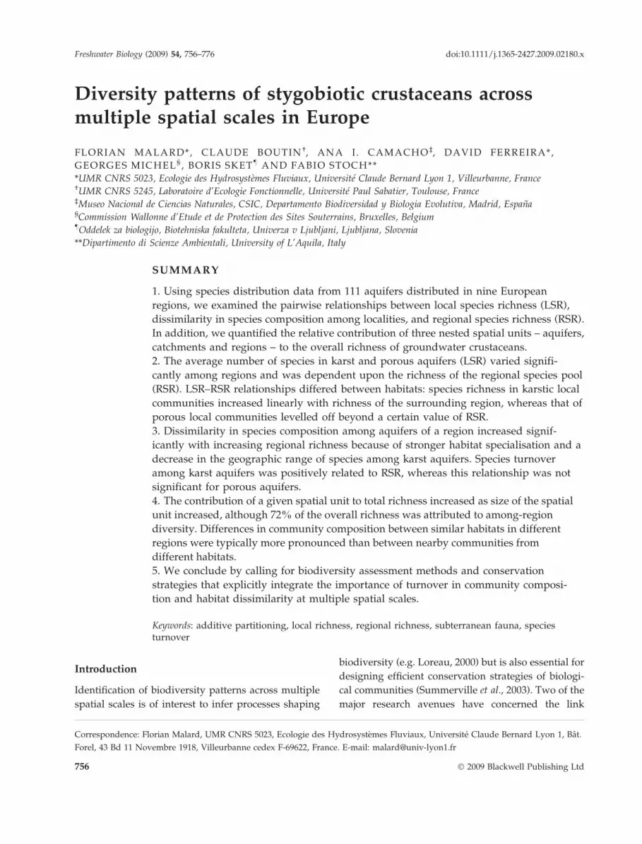
Nine regions were chosen for this study (Fig. 1,
Appendices 1 & 2). We refer to a region as a
relatively large area that experienced a set of similar
historical events (i.e. marine transgression ⁄ regression,
glacial cover and tectonics). Groundwater fauna in
Wallonia (WA), Slovenia (SL), Cantabria (CA) and
the Jura (JU), Roussillon (RO) and Padano-alpine
(a)
(b)
Fig. 1 (a) Physical geography of the study area showing elevation (grey patterns) and extent of glaciers (thick continuous
black line) and permafrost (thick broken black line) during the late glacial maximum (c. 20 000 BP). Limits of glaciers and permafrost
are from Hewitt (1999) and Buoncristiani & Campy (2004), respectively. (b) Location of regions and aquifers (black dots).
758 F. Malard et al.
� 2009 Blackwell Publishing Ltd, Freshwater Biology, 54, 756–776
(PA), regions was sampled as part of the European
research project PASCALIS (Gibert, 2001). Three
additional regions – the Rhone River corridor (RH)
and the Garonne (GA) and Languedoc (LA) regions –
were selected because their groundwater fauna had
been intensively studied at least since the 1970s
(Ferreira et al., 2007). A total of 111 well-studied
aquifers were selected in the nine regions (Fig. 1,
Appendices 1 & 2). An individual aquifer was con-
sidered as an appropriate spatial unit for estimating
local richness. Indeed, aquifers are finite and contin-
uous subsurface hydrological systems within which
organisms can encounter each other and potentially
interact within ecological time. We distinguished
between two different types of aquifers that have
long been considered as distinct groundwater habi-
tats (Gibert et al., 1994a,b). Karst aquifers form within
soluble rock and conduct water principally via a
connected network of fissures, whereas porous aqui-
fers form within unconsolidated sediments (allu-
vium, colluvium, glacial till and outwash) and
conduct water via a connected network of interstices.
The number of aquifers selected in each region varied
from three to nine for karst aquifers and four to eight
for porous aquifers (Appendices 1 & 2). The Langue-
doc and Rhone River regions only comprised karst
(n = 3) and porous aquifers (n = 6), respectively.
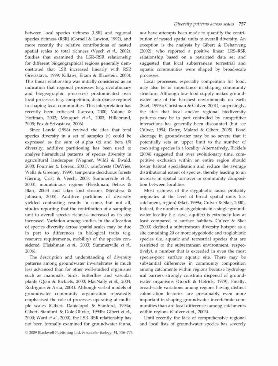
Four regions (WA, JU, RO and CA) were used for
analysing the relative contribution of three nested
spatial units (aquifer, catchment and region) to total
richness (see Data analysis). In these regions, we
selected four distinct river catchments and retained
two karst aquifers and two porous aquifers per
catchment (Fig. 2, Appendices 1 & 2). The boundaries
of regions, catchments and aquifers were delineated
in ARCGISARCGIS 8.3 (ESRI, Redlands, CA, USA) using
multiple coverages including Landsat images, aerial
photographs, digital elevation models and topologi-
cal, hydrological and geological maps. Polygon shape
files of regions, catchments and aquifers are available
upon request from the first author.
Species lists
We assembled a species list of stygobionts as complete
as possible for each aquifer using two distinct data
sets. Stygobionts are obligate groundwater taxa that
complete their entire life cycle exclusively in subsur-
face water (Gibert et al., 1994a) and they represent
approximately 8% of freshwater animal species in
Europe (Sket, 1999b). The first data set consisted in a
presence–absence species table arising from the sam-
pling of 192 sites (i.e. springs, wells, caves and
hyporheic sites) in four river catchments of a region.
This data set was available for the six regions
investigated as part of the PASCALIS project (WA,
JU, RO, CA, PA and SL). Detailed information on the
sampling design and methods are given in Malard
et al. (2002). The second data set was a presence data
base containing 10 183 occurrences of 1059 sty-
gobionts collected in Belgium, France, Italy, Portugal,
Slovenia and Spain (Deharveng et al., 2009). This
‘European data base’ was built based on literature
information, existing national data bases and personal
collections. Both data sets were projected as point
coverages in ARCGISARCGIS 8.3 and intersected with the
polygon coverage of aquifers. Only those data points
that intersected the polygons were analysed. Crusta-
ceans were the only taxonomic group retained for
analysis because other groups appeared to be
unevenly studied in the different regions. Crustaceans
are the dominant group in ground water and
accounted for 71.9% and 80.3%, respectively, of the
species and records included in the European data
base. Epigean species present in ground water were
not considered in the analysis. Lists of stygobiotic
crustacean species, records and distribution maps
were checked by taxonomic group experts to avoid
inconsistencies and synonymies among regions. The
final presence–absence data matrix contained 111
aquifers and 373 crustacean species and subspecies
belonging to 30 families and 78 genera (Table 1). The
dominant families in terms of species richness were
Cyclopidae (Cyclopoida), Niphargidae (Amphipoda),
Canthocamptidae (Harpacticoida) and Candonidae
(Ostracoda).
Fig. 2 Spatial hierarchy considered in the additive
partitioning of species richness. Levels 1 (aquifer), 2
(catchment) and 3 (regions) contained 64, 16 and 4 samples,
respectively. Letters C, K and P designate catchment, karst
aquifers and porous aquifers, respectively.
Diversity patterns across scales 759
� 2009 Blackwell Publishing Ltd, Freshwater Biology, 54, 756–776

Data analysis
Effect of region and RSR on LSR. ANOVAANOVA and Tukey’s
post hoc multiple comparisons were used to test for
differences in LSR between regions and aquifer types
(karst versus porous aquifers). LSR was the mean
number of species in karst or porous aquifers of a
region. A nested design was used to test for the effect
of aquifer type (i.e. aquifer type nested within
regions). Region and aquifer type were used as
random and fixed factors, respectively.
Local species richness was plotted against RSR to
determine whether species richness of an aquifer was
limited by the supply of colonising species from the
surrounding region (Srivastava, 1999). LSR–RSR rela-
tionships were assessed separately for karst (K) and
porous (P) aquifers so that the regional pool of an
aquifer type only comprised species which could
colonise that particular type. We estimated RSR in
two different ways. First, RSR1* was estimated as the
cumulative number of species in the selected aquifers
of a region, excluding locally endemic species. The
use of RSR* instead of RSR (i.e. cumulative number of
species in the aquifers of a region) was advocated by
Cresswell, Vidal-Martinez & Crichton (1995) to ensure
independence between estimates of local and regional
richness. Secondly, RSR2* was calculated for each
region as the total number of groundwater crustacean
species listed in our European data base, again
excluding locally endemic species. We fitted uncon-
strained linear and second-order polynomial regres-
sions to the data and performed a t-test on the
second-order term to test whether the second-order
polynomial gave a better fit than the linear model.
Ideally, RSR–LSR regression lines should pass
through the origin because a region with no species
necessarily has a local richness of zero. However,
constrained regressions extrapolate local richness
beyond the range of the data and inflate R2 values
(but see Srivastava (1999) for a discussion on the
statistical merit of constraining regression lines). We
did not attempt to account for differences in region
size because RSR did not appear to increase with
region size. The number of species in an aquifer did
not correlate positively with aquifer area in any region
except Cantabria.
Relationships between species turnover and RSR. We
examined the relationship between species turnover
among aquifers and RSR using linear regressions.
Pairwise dissimilarity between aquifers i and j was
measured using bsim (Lennon et al., 2001):
bsim ¼min b;cð Þ
min b;cð Þ þ a
where a is the number of species in common for a pair
of aquifers i and j and b and c are the numbers of
species exclusive to aquifer i and j. bsim is considered
as a narrow-sense measure of species turnover
because it focuses more on compositional differences
between aquifers than on differences in species
richness (Lennon et al., 2001; Koleff, Gaston & Len-
non, 2003). It exhibits an upper limit of 1 when
aquifers i and j have no species in common and a
lower limit of 0 when all species belonging to aquifer i
occurs in aquifer j. The average between-aquifer
dissimilarity in species composition for each region
Table 1 Number of genera and species within the crustacean
families present in 111 aquifers distributed in 9 European
regions
Order ⁄ class Family Genus Species
Decapoda Atyiidae 2 3
Amphipoda Bogidiellidae 2 3
Crangonyctidae 2 2
Ingolfiellidae 1 2
Niphargidae 4 58
Pseudoniphargidae 1 4
Salentinellidae 2 9
Isopoda Asellidae 4 20
Cirolanidae 3 4
Microparasellidae 1 11
Sphaeromatidae 2 14
Stenasellidae 1 6
Trichoniscidae 1 1
Thermosbaenacea Thermosbaenidae 1 1
Bathynellacea Bathynellidae 7 21
Parabathynellidae 3 12
Calanoida Diaptomidae 2 2
Cyclopoida Cyclopidae 7 62
Harpacticoida Ameiridae 3 13
Canthocamptidae 11 51
Ectinosomatidae 2 3
Parastenocarididae 1 21
Cladocera Chydoridae 1 2
Ostracoda Candonidae 7 40
Cyprididae 2 2
Cypridopsidae 1 1
Darwinulidae 1 1
Limnocytheridae 1 1
Metacyprinae 1 1
Sphaeromicolidae 1 2
760 F. Malard et al.
� 2009 Blackwell Publishing Ltd, Freshwater Biology, 54, 756–776
was calculated using all species (average bsim) and by
excluding locally endemics (average bsim*). Average
bsim and bsim* were linearly regressed against RSR
and RSR*, respectively. In order to test whether
compositional differences between aquifer types
increase with increasing RSR, the average dissimilar-
ity between karst and porous aquifers of a region was
regressed against RSR and RSR*. Linear relationships
between average dissimilarity and RSR were also
assessed separately for karst and porous aquifers to
examine differences between aquifer types. Signifi-
cance for all statistical tests was accepted at a = 0.05;
analyses were performed with the STATISTICA 6STATISTICA 6
software (Statsoft, Tulsa, OK, U.S.A.) and RR software
packages (R Development Core Team, 2006).
Differences in community composition across scales.
Hierarchical cluster analysis with the bsim measure of
species turnover was used to examine patterns of
dissimilarity among aquifers. Dissimilarity in species
composition was calculated between all pairs of aqui-
fers, and the UPGMA linkage method (unweighted
pair-group method using arithmetic averages) was
used to compute a hierarchical tree in RR software
(R Development Core Team, 2006).
Additive partitioning was applied to species richness
data collected from a design involving three hierarchi-
cal levels (aquifer, catchment and region) to determine
the contribution of each spatial scale to total richness.
We restricted our analysis to four regions in order to
obtain a balanced hierarchical design (Fig. 2). Total
richness in a set of samples (ST) was additively
partitioned into a within-sample component (alpha
diversity, a) and a between-sample component (beta
diversity, b) as follows (Lande, 1996):
ST ¼ aþ b
where
b ¼X
i
qiðST � SiÞ; a ¼X
i
qiSi;
where Si is the number of species in sample i and qi is
the proportional weight associated with sample i.
Alpha and beta diversity were both expressed as
number of species because a was the average richness
within the samples and b was the average amount of
species not found in a single, randomly chosen
sample. In the context of a hierarchy, a at a given
scale was the sum of a and b at the next lower scale
(Veech et al., 2002). Therefore, the following formulae
apply to our hierarchical design: a2(catchments) = a1(aqui-
fers) + b1(aquifers); a3(regions) = a2(catchments) + b2(catchments);
c = a3(regions) + b3(regions); and after substitution,
c = a1(aquifers) + b1(aquifers) + b2(catchments) + b3(regions).
Thus, it was possible to express the proportional
contribution of each level in the hierarchical design to
the total number of species (c).
We used the reshuffling algorithm of the partition
programme (Crist et al., 2003) to test whether the
observed diversity components (a and b) from our
hierarchical design could have been obtained by a
random distribution of sampling units at the next lower
level. The randomisation procedure for each of the
three levels of the hierarchy proceeded as follows: to
test for the significance of a1(aquifers) and b1(aquifers),
species were randomly allocated among aquifers that
belonged to the same catchment. In a separate random-
isation (test of b2(catchments)), aquifers were randomly
distributed among catchments that belonged to the
same region. At last, b3(regions) was tested by randomly
assigning catchments to any region. Randomisations
were repeated 10 000 times to obtain a null distribution
of a and b components. Statistical significance was
assessed by determining the proportion of null values
that were greater or less than the observed components.
Reserve system design. We examined the effects of
species distribution pattern on the design of ground-
water biodiversity reserves using MARXANMARXAN 1.8.6
(University of Queensland, Brisbane, Australia), an
optimisation package paying explicit attention to
patterns of between-site (aquifer) complementarity
(Ball & Possingham, 2001). The adaptive simulated
annealing followed by the summed irreplaceability
heuristic algorithm was used to determine the mini-
mum number and location of aquifers for represent-
ing all species at least once (i.e. full representation
goal). We examined the relationship between the
proportion of aquifers selected in each region and RSR
and average between-aquifer dissimilarity.
Results
Differences in LSR between regions and habitats
Local species richness of karst and porous aquifers
varied significantly between regions (region effect:
Diversity patterns across scales 761
� 2009 Blackwell Publishing Ltd, Freshwater Biology, 54, 756–776
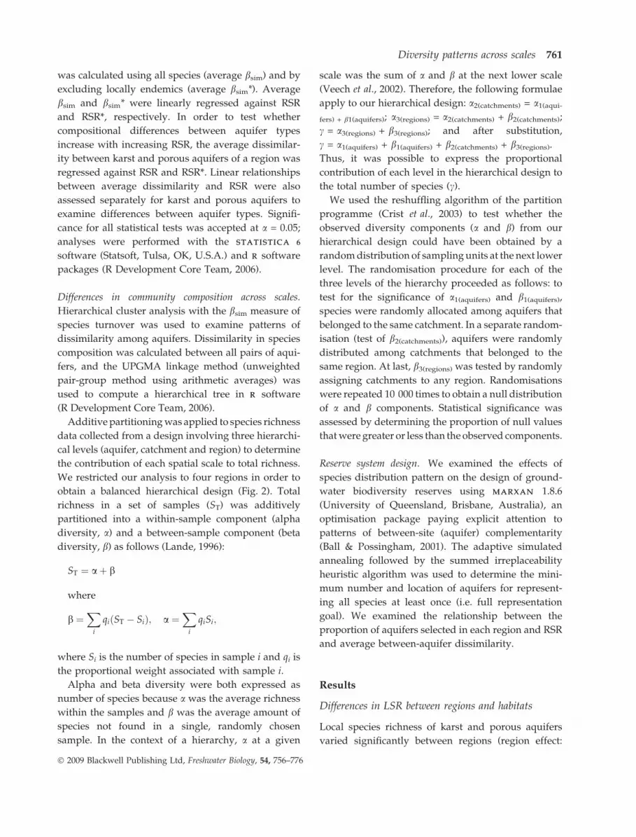
F = 3.06, P = 0.01 for karst aquifers; F = 11, P < 0.001
for porous aquifers; Fig. 3). Species richness of the
Walloon karst aquifers was significantly lower than
that of Slovenian karst aquifers (Tukey’s tests,
P = 0.04). Porous aquifers in Wallonia and Cantabria
contained significantly fewer species than
porous aquifers of all other regions (Tukey’s tests,
P < 0.05). LSR of karst and porous aquifers were
positively correlated across regions (Spearman’s rank
correlation coefficient = 0.94, P = 0.005, n = 6;
Cantabria excluded). Porous aquifers contained in
average more species than karst aquifers (hierarchical
ANOVAANOVA, aquifer type nested in region, F7,88 = 3.04,
P = 0.006).
LSR–RSR relationships
None of the regional species–accumulation curves
(cumulative species richness versus number of
aquifers) performed with EstimateS (Colwell, 2005)
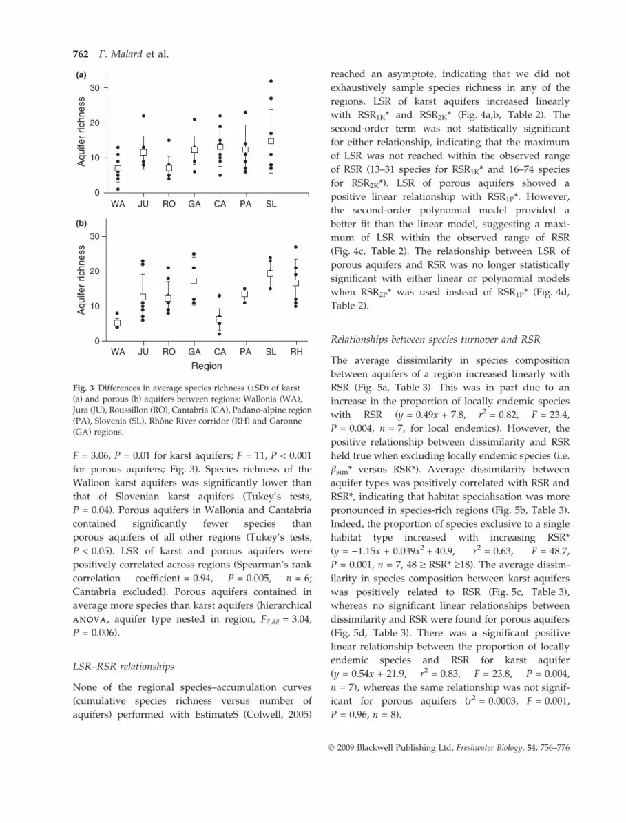
reached an asymptote, indicating that we did not
exhaustively sample species richness in any of the
regions. LSR of karst aquifers increased linearly
with RSR1K* and RSR2K* (Fig. 4a,b, Table 2). The
second-order term was not statistically significant
for either relationship, indicating that the maximum
of LSR was not reached within the observed range
of RSR (13–31 species for RSR1K* and 16–74 species
for RSR2K*). LSR of porous aquifers showed a
positive linear relationship with RSR1P*. However,
the second-order polynomial model provided a
better fit than the linear model, suggesting a maxi-
mum of LSR within the observed range of RSR
(Fig. 4c, Table 2). The relationship between LSR of
porous aquifers and RSR was no longer statistically
significant with either linear or polynomial models
when RSR2P* was used instead of RSR1P* (Fig. 4d,
Table 2).
Relationships between species turnover and RSR
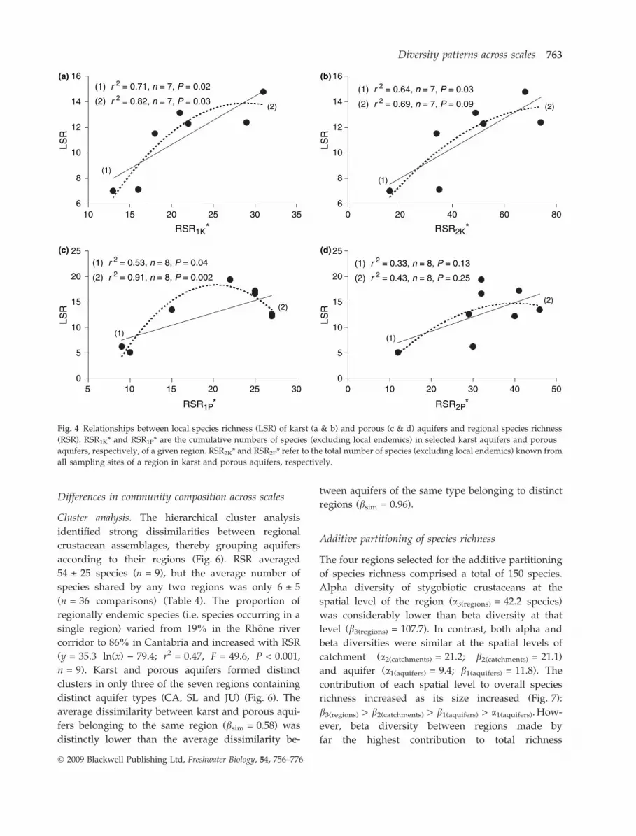
The average dissimilarity in species composition
between aquifers of a region increased linearly with
RSR (Fig. 5a, Table 3). This was in part due to an
increase in the proportion of locally endemic species
with RSR (y = 0.49x + 7.8, r2 = 0.82, F = 23.4,
P = 0.004, n = 7, for local endemics). However, the
positive relationship between dissimilarity and RSR
held true when excluding locally endemic species (i.e.
bsim* versus RSR*). Average dissimilarity between
aquifer types was positively correlated with RSR and
RSR*, indicating that habitat specialisation was more
pronounced in species-rich regions (Fig. 5b, Table 3).
Indeed, the proportion of species exclusive to a single
habitat type increased with increasing RSR*
(y = )1.15x + 0.039x2 + 40.9, r2 = 0.63, F = 48.7,
P = 0.001, n = 7, 48 ‡ RSR* ‡18). The average dissim-
ilarity in species composition between karst aquifers
was positively related to RSR (Fig. 5c, Table 3),
whereas no significant linear relationships between
dissimilarity and RSR were found for porous aquifers
(Fig. 5d, Table 3). There was a significant positive
linear relationship between the proportion of locally
endemic species and RSR for karst aquifer
(y = 0.54x + 21.9, r2 = 0.83, F = 23.8, P = 0.004,
n = 7), whereas the same relationship was not signif-
icant for porous aquifers (r2 = 0.0003, F = 0.001,
P = 0.96, n = 8).
30
(a)
(b)
20
10
0
30
20
10
0
Region
Aqu
ifer
richn
ess
Aqu
ifer
richn
ess
CA
CA RH
GA
GA
JU
JU
SL
SL
PA
PA
RO
RO
WA
WA
Fig. 3 Differences in average species richness (±SD) of karst
(a) and porous (b) aquifers between regions: Wallonia (WA),
Jura (JU), Roussillon (RO), Cantabria (CA), Padano-alpine region
(PA), Slovenia (SL), Rhone River corridor (RH) and Garonne
(GA) regions.
762 F. Malard et al.
� 2009 Blackwell Publishing Ltd, Freshwater Biology, 54, 756–776
Differences in community composition across scales
Cluster analysis. The hierarchical cluster analysis
identified strong dissimilarities between regional
crustacean assemblages, thereby grouping aquifers
according to their regions (Fig. 6). RSR averaged
54 ± 25 species (n = 9), but the average number of
species shared by any two regions was only 6 ± 5
(n = 36 comparisons) (Table 4). The proportion of
regionally endemic species (i.e. species occurring in a
single region) varied from 19% in the Rhone river
corridor to 86% in Cantabria and increased with RSR
(y = 35.3 ln(x) ) 79.4; r2 = 0.47, F = 49.6, P < 0.001,
n = 9). Karst and porous aquifers formed distinct
clusters in only three of the seven regions containing
distinct aquifer types (CA, SL and JU) (Fig. 6). The
average dissimilarity between karst and porous aqui-
fers belonging to the same region (bsim = 0.58) was
distinctly lower than the average dissimilarity be-
tween aquifers of the same type belonging to distinct
regions (bsim = 0.96).
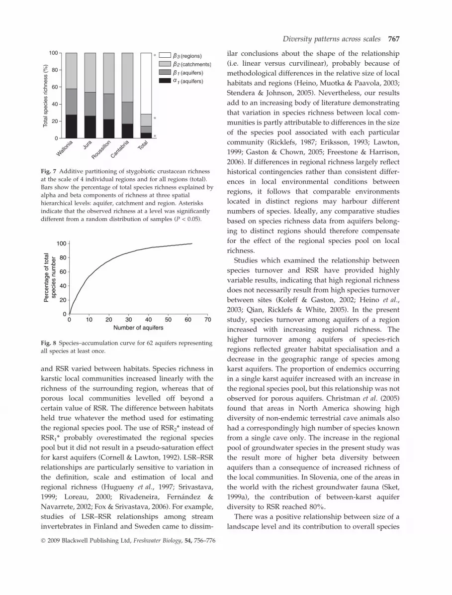
Additive partitioning of species richness
The four regions selected for the additive partitioning
of species richness comprised a total of 150 species.
Alpha diversity of stygobiotic crustaceans at the
spatial level of the region (a3(regions) = 42.2 species)
was considerably lower than beta diversity at that
level (b3(regions) = 107.7). In contrast, both alpha and
beta diversities were similar at the spatial levels of
catchment (a2(catchments) = 21.2; b2(catchments) = 21.1)
and aquifer (a1(aquifers) = 9.4; b1(aquifers) = 11.8). The
contribution of each spatial level to overall species
richness increased as its size increased (Fig. 7):
b3(regions) > b2(catchments) > b1(aquifers) > a1(aquifers). How-
ever, beta diversity between regions made by
far the highest contribution to total richness
14
12
10
8
6
16(a) (b)
(c) (d)
14
12
10
8
6
16
20
15
10
5
0252015105
3025201510 806040200
25
20
15
10
5
0
25
LSR
LSR
LSR
LSR
RSR2K*RSR1K*
RSR2P*RSR1P*
(1) r 2 = 0.71, n = 7, P = 0.02
(2) r 2 = 0.82, n = 7, P = 0.03
30 403020100 50
35
(1) r 2 = 0.53, n = 8, P = 0.04
(2) r 2 = 0.91, n = 8, P = 0.002
(1) r 2 = 0.33, n = 8, P = 0.13
(2) r 2 = 0.43, n = 8, P = 0.25
(1) r 2 = 0.64, n = 7, P = 0.03
(2) r 2 = 0.69, n = 7, P = 0.09
(1)
(2)
(1)
(2)
(1)
(2)
(1)
(2)
Fig. 4 Relationships between local species richness (LSR) of karst (a & b) and porous (c & d) aquifers and regional species richness
(RSR). RSR1K* and RSR1P* are the cumulative numbers of species (excluding local endemics) in selected karst aquifers and porous
aquifers, respectively, of a given region. RSR2K* and RSR2P* refer to the total number of species (excluding local endemics) known from
all sampling sites of a region in karst and porous aquifers, respectively.
Diversity patterns across scales 763
� 2009 Blackwell Publishing Ltd, Freshwater Biology, 54, 756–776

Table 2 Coefficients with standard errors (SE), t statistic and significance level (P) of the linear and second-order polynomial
regression models for the relationship between LSR and RSR (see Fig. 4)
Habitat RSR Model n Term Coefficient SE t P-value
Karst RSR1K* Linear 7 Constant 3.0 2.4 1.24 0.27
First order 0.4 0.1 3.47 0.02
Polynomial 7 Constant )10.7 8.9 )1.21 0.29
First order 1.7 0.8 2.04 0.11
Second order 0.0 0.0 )1.59 0.19
RSR2K* Linear 7 Constant 5.6 2.0 2.84 0.04
First order 0.1 0.0 2.99 0.03
Polynomial 7 Constant 2.3 4.5 0.53 0.63
First order 0.3 0.2 1.38 0.24
Second order 0.0 0.0 )0.83 0.45
Porous RSR1p* Linear 8 Constant 3.1 4.0 0.77 0.47
First order 0.5 0.2 2.59 0.04
Polynomial 8 Constant )27.0 6.6 )4.09 0.009
First order 4.5 0.8 5.31 0.003
Second order )0.1 0.0 )4.75 0.005
RSR2p* Linear 8 Constant 3.6 5.6 0.65 0.54
First order 0.3 0.2 1.73 0.13
Polynomial 8 Constant )5.6 11.5 )0.49 0.64
First order 1.0 0.8 1.25 0.26
Second order 0.0 0.0 )0.92 0.40
Fig. 5 Relationships between species turnover among aquifers (average bsim expressed as a percentage) and regional species
richness (RSR). Dissimilarity between (a) all aquifers of a region, (b) karst and porous aquifers, (c) karst aquifers and (d) porous aquifers.
bsim and bsim* were regressed against RSR and RSR*, respectively.
764 F. Malard et al.
� 2009 Blackwell Publishing Ltd, Freshwater Biology, 54, 756–776
(b3(regions) = 71.8%). The proportion of species unique
to an aquifer, a catchment, and a region was 29%,
41% and 89%, respectively. The observed diversity
within aquifers (a1), between catchments (b2) and
between regions (b3) was always greater than
expected by chance (P < 0.001), whereas the observed
diversity between aquifers (b1) was not significantly
different (P = 0.13) from a random distribution of
species among aquifers.
The proportions of richness components varied
little among regions (Fig. 7). Between-catchment
diversity (b2) was typically higher than both be-
tween-aquifer (b1) and within aquifer (a1) diversity.
The contribution of between-catchment diversity (b2)
to regional richness increased in the order Wallonia,
Jura, Roussillon and Cantabria, whereas that of
within-aquifer diversity (a1) showed the reverse
order.
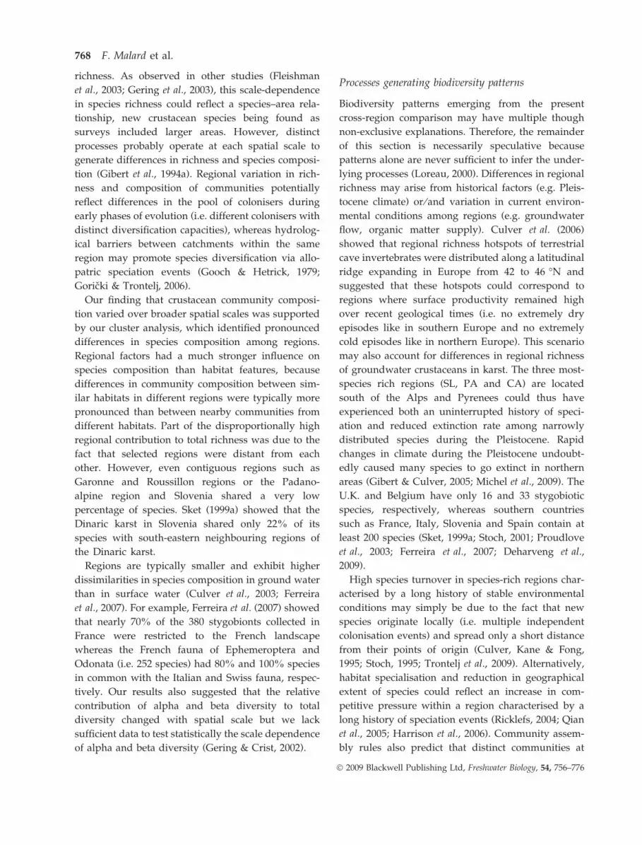
Reserve system design
Of a total of 111 aquifers, 62 were needed to capture
all species at least once, although a high proportion of
species rapidly accumulated in relatively few aquifers
(Fig. 8). The full representation goal was achieved by
selecting dissimilar proportions of aquifers in each
region. The proportion of selected aquifers in a region
increased linearly with RSR (y = 1.04x ) 1.67,
r2 = 0.82, F = 22.7, P = 0.005, n = 7) and bsim
(y = 2.37x ) 77.12, r2 = 0.93, F = 70.5, P < 0.001,
n = 7). Of a total of 373 species, 303 (81%) were
represented in only 24 species-rich aquifers unevenly
distributed in distinct regions: six aquifers in Slovenia;
four in the Padano-alpine region; three each in
Cantabria, the Garonne Basin and Roussillon; two in
the Jura and one in Wallonia, the Languedoc and
Rhone River corridor. These 24 species-rich aquifers
comprised 16 karst aquifers (27% of karst aquifers)
and only seven porous aquifers (i.e. 14% of porous
aquifers).
Discussion
Emerging patterns of groundwater biodiversity
Several interesting patterns emerge from the present
study on relationships between local richness and
species turnover and regional richness of groundwa-
ter communities across nine European regions. Some
regions (e.g. Slovenia) contained on average signifi-
cantly more species of crustaceans per aquifer than
others (e.g. Wallonia). Species richness of karst and
porous aquifers covaried among regions but the
average number of species in porous aquifers was
higher than that of karst aquifers. This latter result is
counterintuitive because karst aquifers offer older and
more heterogeneous habitats than porous aquifers.
The average number of species per aquifer (LSR)
was dependent upon the richness of the regional
species pool (RSR), but the relationship between LSR
Table 3 Coefficients with standard errors (SE), t statistic and significance level (P) of the linear regression models for the
relationship between turnover in species composition among aquifers and RSR (see Fig. 5)
Aquifers
Local
endemics n Term Coefficient SE t P-value
All Yes 7 Constant 32.0 4.8 6.60 0.001
RSR 0.4 0.1 5.67 0.002
No 7 Constant 19.2 8.6 2.22 0.08
RSR* 1.0 0.2 3.92 0.01
Karst and
porous
Yes 7 Constant 31.5 2.1 14.90 <0.001
RSR 0.5 0.0 14.62 <0.001
No 7 Constant 11.4 6.2 1.84 0.12
RSR* 1.3 0.2 7.37 0.001
Karst Yes 7 Constant 22.9 11.0 2.08 0.09
RSR1K 0.7 0.2 3.08 0.03
No 7 Constant 5.7 11.8 0.48 0.64
RSR1K* 1.9 0.5 3.51 0.02
Porous Yes 8 Constant 57.6 12.1 4.77 0.003
RSR1P )0.3 0.3 )0.82 0.44
No 8 Constant 46.7 8.3 5.66 0.001
RSR1P* )0.5 0.4 )1.23 0.26
Diversity patterns across scales 765
� 2009 Blackwell Publishing Ltd, Freshwater Biology, 54, 756–776
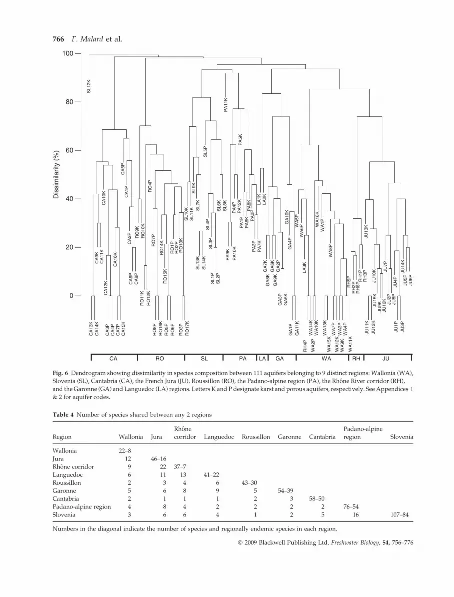
Fig. 6 Dendrogram showing dissimilarity in species composition between 111 aquifers belonging to 9 distinct regions: Wallonia (WA),
Slovenia (SL), Cantabria (CA), the French Jura (JU), Roussillon (RO), the Padano-alpine region (PA), the Rhone River corridor (RH),
and the Garonne (GA) and Languedoc (LA) regions. Letters K and P designate karst and porous aquifers, respectively. See Appendices 1
& 2 for aquifer codes.
Table 4 Number of species shared between any 2 regions
Region Wallonia Jura
Rhone
corridor Languedoc Roussillon Garonne Cantabria
Padano-alpine
region Slovenia
Wallonia 22–8
Jura 12 46–16
Rhone corridor 9 22 37–7
Languedoc 6 11 13 41–22
Roussillon 2 3 4 6 43–30
Garonne 5 6 8 9 5 54–39
Cantabria 2 1 1 1 2 3 58–50
Padano-alpine region 4 8 4 2 2 2 2 76–54
Slovenia 3 6 6 4 1 2 5 16 107–84
Numbers in the diagonal indicate the number of species and regionally endemic species in each region.
766 F. Malard et al.
� 2009 Blackwell Publishing Ltd, Freshwater Biology, 54, 756–776
and RSR varied between habitats. Species richness in
karstic local communities increased linearly with the
richness of the surrounding region, whereas that of
porous local communities levelled off beyond a
certain value of RSR. The difference between habitats
held true whatever the method used for estimating
the regional species pool. The use of RSR2* instead of
RSR1* probably overestimated the regional species
pool but it did not result in a pseudo-saturation effect
for karst aquifers (Cornell & Lawton, 1992). LSR–RSR
relationships are particularly sensitive to variation in
the definition, scale and estimation of local and
regional richness (Hugueny et al., 1997; Srivastava,
1999; Loreau, 2000; Rivadeneira, Fernandez &
Navarrete, 2002; Fox & Srivastava, 2006). For example,
studies of LSR–RSR relationships among stream
invertebrates in Finland and Sweden came to dissim-
ilar conclusions about the shape of the relationship
(i.e. linear versus curvilinear), probably because of
methodological differences in the relative size of local
habitats and regions (Heino, Muotka & Paavola, 2003;
Stendera & Johnson, 2005). Nevertheless, our results
add to an increasing body of literature demonstrating
that variation in species richness between local com-
munities is partly attributable to differences in the size
of the species pool associated with each particular
community (Ricklefs, 1987; Eriksson, 1993; Lawton,
1999; Gaston & Chown, 2005; Freestone & Harrison,
2006). If differences in regional richness largely reflect
historical contingencies rather than consistent differ-
ences in local environmental conditions between
regions, it follows that comparable environments
located in distinct regions may harbour different
numbers of species. Ideally, any comparative studies
based on species richness data from aquifers belong-
ing to distinct regions should therefore compensate
for the effect of the regional species pool on local
richness.
Studies which examined the relationship between
species turnover and RSR have provided highly
variable results, indicating that high regional richness
does not necessarily result from high species turnover
between sites (Koleff & Gaston, 2002; Heino et al.,
2003; Qian, Ricklefs & White, 2005). In the present
study, species turnover among aquifers of a region
increased with increasing regional richness. The
higher turnover among aquifers of species-rich
regions reflected greater habitat specialisation and a
decrease in the geographic range of species among
karst aquifers. The proportion of endemics occurring
in a single karst aquifer increased with an increase in
the regional species pool, but this relationship was not
observed for porous aquifers. Christman et al. (2005)
found that areas in North America showing high
diversity of non-endemic terrestrial cave animals also
had a correspondingly high number of species known
from a single cave only. The increase in the regional
pool of groundwater species in the present study was
the result more of higher beta diversity between
aquifers than a consequence of increased richness of
the local communities. In Slovenia, one of the areas in
the world with the richest groundwater fauna (Sket,
1999a), the contribution of between-karst aquifer
diversity to RSR reached 80%.
There was a positive relationship between size of a
landscape level and its contribution to overall species
Fig. 7 Additive partitioning of stygobiotic crustacean richness
at the scale of 4 individual regions and for all regions (total).
Bars show the percentage of total species richness explained by
alpha and beta components of richness at three spatial
hierarchical levels: aquifer, catchment and region. Asterisks
indicate that the observed richness at a level was significantly
different from a random distribution of samples (P < 0.05).
0
60
40
20
0 605040302010 70
80
100
Number of aquifers
Per
cent
age
of to
tal
spec
ies
num
ber
Fig. 8 Species–accumulation curve for 62 aquifers representing
all species at least once.
Diversity patterns across scales 767
� 2009 Blackwell Publishing Ltd, Freshwater Biology, 54, 756–776
richness. As observed in other studies (Fleishman
et al., 2003; Gering et al., 2003), this scale-dependence
in species richness could reflect a species–area rela-
tionship, new crustacean species being found as
surveys included larger areas. However, distinct
processes probably operate at each spatial scale to
generate differences in richness and species composi-
tion (Gibert et al., 1994a). Regional variation in rich-
ness and composition of communities potentially
reflect differences in the pool of colonisers during
early phases of evolution (i.e. different colonisers with
distinct diversification capacities), whereas hydrolog-
ical barriers between catchments within the same
region may promote species diversification via allo-
patric speciation events (Gooch & Hetrick, 1979;
Goricki & Trontelj, 2006).
Our finding that crustacean community composi-
tion varied over broader spatial scales was supported
by our cluster analysis, which identified pronounced
differences in species composition among regions.
Regional factors had a much stronger influence on
species composition than habitat features, because
differences in community composition between sim-
ilar habitats in different regions were typically more
pronounced than between nearby communities from
different habitats. Part of the disproportionally high
regional contribution to total richness was due to the
fact that selected regions were distant from each
other. However, even contiguous regions such as
Garonne and Roussillon regions or the Padano-
alpine region and Slovenia shared a very low
percentage of species. Sket (1999a) showed that the
Dinaric karst in Slovenia shared only 22% of its
species with south-eastern neighbouring regions of
the Dinaric karst.
Regions are typically smaller and exhibit higher
dissimilarities in species composition in ground water
than in surface water (Culver et al., 2003; Ferreira
et al., 2007). For example, Ferreira et al. (2007) showed
that nearly 70% of the 380 stygobionts collected in
France were restricted to the French landscape
whereas the French fauna of Ephemeroptera and
Odonata (i.e. 252 species) had 80% and 100% species
in common with the Italian and Swiss fauna, respec-
tively. Our results also suggested that the relative
contribution of alpha and beta diversity to total
diversity changed with spatial scale but we lack
sufficient data to test statistically the scale dependence
of alpha and beta diversity (Gering & Crist, 2002).
Processes generating biodiversity patterns
Biodiversity patterns emerging from the present
cross-region comparison may have multiple though
non-exclusive explanations. Therefore, the remainder
of this section is necessarily speculative because
patterns alone are never sufficient to infer the under-
lying processes (Loreau, 2000). Differences in regional
richness may arise from historical factors (e.g. Pleis-
tocene climate) or ⁄and variation in current environ-
mental conditions among regions (e.g. groundwater
flow, organic matter supply). Culver et al. (2006)
showed that regional richness hotspots of terrestrial
cave invertebrates were distributed along a latitudinal
ridge expanding in Europe from 42 to 46 �N and
suggested that these hotspots could correspond to
regions where surface productivity remained high
over recent geological times (i.e. no extremely dry
episodes like in southern Europe and no extremely
cold episodes like in northern Europe). This scenario
may also account for differences in regional richness
of groundwater crustaceans in karst. The three most-
species rich regions (SL, PA and CA) are located
south of the Alps and Pyrenees could thus have
experienced both an uninterrupted history of speci-
ation and reduced extinction rate among narrowly
distributed species during the Pleistocene. Rapid
changes in climate during the Pleistocene undoubt-
edly caused many species to go extinct in northern
areas (Gibert & Culver, 2005; Michel et al., 2009). The
U.K. and Belgium have only 16 and 33 stygobiotic
species, respectively, whereas southern countries
such as France, Italy, Slovenia and Spain contain at
least 200 species (Sket, 1999a; Stoch, 2001; Proudlove
et al., 2003; Ferreira et al., 2007; Deharveng et al.,
2009).
High species turnover in species-rich regions char-
acterised by a long history of stable environmental
conditions may simply be due to the fact that new
species originate locally (i.e. multiple independent
colonisation events) and spread only a short distance
from their points of origin (Culver, Kane & Fong,
1995; Stoch, 1995; Trontelj et al., 2009). Alternatively,
habitat specialisation and reduction in geographical
extent of species could reflect an increase in com-
petitive pressure within a region characterised by a
long history of speciation events (Ricklefs, 2004; Qian
et al., 2005; Harrison et al., 2006). Community assem-
bly rules also predict that distinct communities at
768 F. Malard et al.
� 2009 Blackwell Publishing Ltd, Freshwater Biology, 54, 756–776
environmentally similar sites, which leads to high
species turnover, are more likely to occur in regions
with high productivity, large species pools and low
dispersal rates (Chase, 2003).
Differences in diversity patterns between karst and
porous communities suggest that composition of
these communities might be controlled by different
factors. Part of the variation potentially resides in the
expectedly higher hydrological connectivity between
porous aquifers (Ward & Palmer, 1994). Greater
connectivity may promote dispersal, which reduces
species turnover among localities and enables coloni-
sation of most localities by competitively superior
species (Chase, 2003). Dispersal may simultaneously
decrease differences in species composition among
localities and decrease extinction rates, resulting in a
negative relationship between regional richness and
species turnover (Hunter, 2005). Dissimilarities in
species composition among porous aquifers were
indeed lower than between karstic aquifers, although
the difference was not statistically significant. Clearly,
additional distribution data are needed to elucidate
diversity patterns of fauna in porous aquifers and
formulate testable scenarios that can explain the
origin of these patterns.
Implications for biodiversity assessment and
conservation
Determining conservation strategies requires that at
least diversity patterns, if not the processes that
determine them, are identified at multiple spatial
scales (Summerville et al., 2003). Many of the patterns
revealed in the present study have important impli-
cations for the assessment and conservation of
groundwater biodiversity. The additive partitioning
of groundwater biodiversity indicates that ground-
water species–accumulation curves are unlikely to
saturate in spatially extensive sampling designs
because beta diversity becomes increasingly large
with increasing spatial scale. Interestingly, although
groundwater ecologists deal with species-poor com-
munities, they are confronted with the same dilemma
as biologists involved in the conservation of hyperdi-
verse communities (Gering et al., 2003). Complete
inventories yielding saturated species–accumulation
curves can only be achieved by intensive sampling of
a limited spatial area (Rouch & Danielopol, 1997;
Pipan & Culver, 2007) but such surveys provide poor
indications of the spatial variation in community
composition. Extensive regional sampling will yield
unsaturated accumulation curves (Castellarini et al.,
2007; Dole-Olivier et al., 2009) but a better estimate of
the contribution of species turnover to overall ground-
water diversity.
Effective protection of groundwater fauna necessi-
tates a conservation strategy that specifically consid-
ers patterns of species replacement at multiple spatial
scales. Indeed, beta diversity was at least as important
as alpha diversity in determining total richness at the
spatial scales of the aquifer in the present analysis
(b1(aquifers) = 56%), catchment (b2(catchments) = 50%)
and region (b3(regions) = 72%). Several studies which
examined patterns of diversity among a variety of
organisms showed that regional diversity was influ-
enced to a greater extent by beta diversity (Harrison &
Inouye, 2002; Culver et al., 2003; Pineda & Halffter,
2004; Rodriguez & Arita, 2004). A number of reserve
selection algorithms paying explicit attention to
between-site complementarity have recently been
developed and could be used for maximising the
representation of groundwater species in a network of
aquifers at the European scale (Fischer & Church,
2005; Michel et al., 2009).
A more precise delineation of groundwater ecore-
gions using methods such as clustering techniques
(see e.g. Houghton, 2004; Proches, 2005; Hahn &
Fuchs, 2009) is essential for conservation planning in
Europe because the diversity of groundwater fauna
arises largely from species turnover among regions.
The global biogeographical scheme by Botosaneanu
(1986) is one of the first approaches to regionalising
groundwater organism distributions but it is yet much
too coarse to be used for conservation purpose. The
disproprotionally high contribution of between-re-
gions to overall richness implies that a high propor-
tion of groundwater species in Europe can be
protected by focusing conservation efforts on a few
aquifers distributed in distinct regions. Indeed, the
few attempts made to identify areas to be reserved for
representing species at large spatial scales showed
that a very small proportion of the groundwater
landscape (<2%) was needed to capture the majority
of species (Culver et al., 2000; Ferreira et al., 2007;
Michel et al., 2009). A proportionally higher number
of sites should be selected in species-rich regions
because of the higher contribution of beta diversity
to overall regional diversity. Focusing conservation
Diversity patterns across scales 769
� 2009 Blackwell Publishing Ltd, Freshwater Biology, 54, 756–776

effort on species-rich regions containing a high num-
ber of endemics is a meaningful strategy because the
restriction of species distribution ranges increases
vulnerability to extinction.
Conservation efforts of groundwater fauna have
essentially been devoted to karst habitats, probably
because of a long history of biological data collection
in caves (Camacho, 1992; Juberthie, 1995). However,
faunal dissimilarities among karst and porous habi-
tats contribute importantly to regional richness. In the
present study, species observed exclusively in karst
and porous aquifers represented on average 37 ± 18%
and 27 ± 11%, respectively, of the regional species
pool (n = 7 regions). The design of reserves based on
the diversity of only one of these aquifer types or the
other will provide very different scenarios for
conservation areas because there is no significant
relationship between regional richness of karst and
porous communities (P = 0.16, n = 7 regions).
Clearly, an effective conservation strategy needs to
consider multiple groundwater habitats because their
relative contribution to gamma diversity varies
among regions.
Acknowledgments
We thank D. Galassi, P. Marmonier and A. Valdeca-
sas for checking consistency in species lists between
selected aquifers. We are indebted to the scientists
who provided georeferenced maps of regions, catch-
ments and aquifers: N. Coineau and M. Artheau
(Roussillon), C. Puch (Cantabrica) and M. Zagmajster
(Slovenia). We thank T. Crist and B. Hugueny for
their valuable help with the additive partition of
groundwater biodiversity and D.C. Culver and two
anonymous reviewers for comments that improved
earlier versions of this manuscript. This work was
supported by the European programme PASCALIS
(Protocols for the ASsessment and Conservation of
Aquatic Life In the Subsurface; contract no. EVK2-
CT-2001-00121).
References
Ball J.R. & Possingham H.P. (2001) The design of marine
protected areas: adapting terrestrial techniques. In:
Proceedings of the International Congress on Modelling and
Simulation. Natural Systems, Vol. 2 (Eds F. Ghassemi,
P. Whetton, R. Little & M. Littleboy), pp. 769–774. The
Modelling and Simulation Society of Australia and
New Zealand Inc., Canberra.
Botosaneanu L. (1986) Stygofauna Mundi, Brill, E.J. and
Dr. W. Backhuys, Leiden, The Netherlands.
Buoncristiani J. & Campy M. (2004) The palaeogeogra-
phy of the last two glacial episodes in France: The Alps
and Jura. In: Quaternary Glaciations – Extent and
Chronology. Part I: Europe (Eds J. Ehlers & P.L.
Gibbard), pp. 101–110. Eslevier, Amsterdam.
Camacho A.I. (1992) The Natural History of Biospeology.
Museo Nacional de Ciencas Naturales, Madrid.
Castellarini F., Dole-Olivier M.-J., Malard F. & Gibert J.
(2007) Using habitat heterogeneity to assess stygobiotic
species richness in the French Jura region with a
conservation perspective. Fundamental and Applied
Limnology, 169, 69–78.
Chase J.M. (2003) Community assembly: when should
history matter? Oecologia, 136, 489–498.
Christman M.C. & Culver D.C. (2001) The relationship
between cave biodiversity and available habitat. Jour-
nal of Biogeography, 28, 367–380.
Christman M.C., Culver D.C., Madden M.K. & White D.
(2005) Patterns of endemism of the eastern North
American cave fauna. Journal of Biogeography, 32, 1441–
1452.
Colwell R.K. (2005) EstimateS: Statistical Estimation of
Species Richness and Shared Species from Samples, Version
7.5. Available at: http://purl.oclc.org/estimates.
Cornell H.V. & Lawton J.H. (1992) Species interactions,
local and regional processes, and limits to the richness
of ecological communities: a theoretical perspective.
Journal of Animal Ecology, 61, 1–12.
Cresswell J.E., Vidal-Martinez V.M. & Crichton N.J.
(1995) The investigation of saturation in the species
richness of communities: some comments on method-
ology. Oikos, 72, 301–304.
Crist T.O., Veech J.A., Gering J.C. & Summerville K.S.
(2003) Partitioning species diversity across landscapes
and regions: a hierarchical analysis of a, b, and cdiversity. American Naturalist, 162, 734–743.
Culver D.C. (1994) Species interactions. In: Groundwater
Ecology (Eds J. Gibert, D.L. Danielopol & J.A. Stanford),
pp. 271–285. Academic Press, New York.
Culver D.C. & Fong D.W. (1994) Small scale and large
scale biogeography of subterranean crustacean faunas
of the Virginias. Hydrobiologia, 287, 3–10.
Culver D.C. & Sket B. (2000) Hotspots of subterranean
biodiversity in caves and wells. Journal of Cave and
Karst Studies, 62, 11–17.
Culver D.C., Kane T.C. & Fong D.W. (1995) Adaptation
and Natural Selection in Caves. The Evolution of Gamm-
arus minus. Harvard University Press, Cambridge, MA.
770 F. Malard et al.
� 2009 Blackwell Publishing Ltd, Freshwater Biology, 54, 756–776

Culver D.C., Master L.L., Christman M.C. & Hobbs H.H.
III (2000) Obligate cave fauna of the 48 contiguous
United States. Conservation Biology, 14, 386–401.
Culver D.C., Christman M.C., Elliott W.R., Hobbs H.H.
III & Reddell J.R. (2003) The North American cave
fauna: regional patterns. Biodiversity and Conservation,
12, 441–468.
Culver D.C., Deharveng L., Bedos A., Lewis J.L., Madden
M., Reddell J.R., Sket B., Trontelj P. & White D. (2006)
The mid-latitude biodiversity ridge in terrestrial cave
fauna. Ecography, 29, 120–128.
Datry T., Malard F. & Gibert J. (2005) Response of
invertebrate assemblages to increased groundwater
recharge rates in a phreatic aquifer. Journal of the North
American Benthological Society, 24, 461–477.
Deharveng L., Stoch F., Gibert J. et al. (2009) Groundwa-
ter biodiversity in Europe. Freshwater Biology, 54, 709–
726.
DeVries P.J., Walla T.R. & Greeney H.F. (1999) Species
diversity in spatial and temporal dimensions of fruit-
feeding butterflies from two Ecuadorian rainforests.
Biological Journal of the Linnean Society, 68, 333–353.
Dole-Olivier M.J., Castellarini F., Coineau N., Galassi
D.M.P., Martin P., Mori N., Valdecasas A. & Gibert J.
(2009) Towards an optimal sampling strategy to assess
groundwater biodiversity: comparison across six
European regions. Freshwater Biology, 54, 777–796.
Eriksson O. (1993) The species–pool hypothesis and plant
community diversity. Oikos, 68, 371–374.
Ferreira D., Malard F., Dole-Olivier M.-J. & Gibert J.
(2007) Obligate groundwater fauna of France: species
richness patterns and conservation implications. Bio-
diversity and Conservation, 16, 567–596.
Fischer D.T. & Church R.L. (2005) The SITES reserve
selection system: a critical review. Environmental Mod-
eling and Assessment, 10, 215–228.
Fleishman E., Betrus C.J. & Blair R.B. (2003) Effects of
spatial scale and taxonomic group on partitioning of
butterfly and bird diversity in the Great Basin, U.S.A.
Landscape Ecology, 18, 675–685.
Fournier E. & Loreau M. (2001) Respective roles of
recent hedges and forest patch remnants in the
maintenance of ground-beetle (Coleoptera: Carabidae)
diversity in an agricultural landscape. Landscape
Ecology, 16, 17–32.
Fox J.W. & Srivastava D. (2006) Predicting local–regional
richness relationships using island biogeography mod-
els. Oikos, 113, 376–382.
Freestone A.L. & Harrison S. (2006) Regional enrichment
of local assemblages is robust to variation in local
productivity, abiotic gradients, and heterogeneity.
Ecology Letters, 9, 95–102.
Gaston K.J. & Chown S.L. (2005) Neutrality and the
niche. Functional Ecology, 19, 1–6.
Gering J.C. & Crist T.O. (2002) The alpha–beta-regional
relationship: providing new insights into local–regio-
nal patterns of species richness and scale dependence
of diversity components. Ecology Letters, 5, 433–444.
Gering J.C., Crist T.O. & Veech J.A. (2003) Additive
partitioning of species diversity across multiple spatial
scales: implications for regional conservation of biodi-
versity. Conservation Biology, 17, 488–499.
Gibert J. (2001) Protocols for the assessment and conser-
vation of aquatic life in the subsurface (PASCALIS): a
European project. In: Mapping Subterranean Biodiversity
(Eds D.C. Culver, L. Deharveng, J. Gibert & I.D.
Sasowsky), pp. 19–21. Special Publication 6, Karst
Waters Institute, Charles Town, VA.
Gibert J., Culver D.C. (2005) Diversity Patterns in
Europe. In: Encyclopedia of Caves (Eds D.C. Culver &
W.B. White), pp. 196–201. Elsevier Academic Press,
New York,
Gibert J. & Deharveng L. (2002) Subterranean ecosys-
tems: a truncated functional biodiversity. BioScience,
52, 473–481.
Gibert J., Stanford J.A., Dole-Olivier M.-J. & Ward V.J.
(1994a) Basic Attributes of Groundwater Ecosystems
and Prospects for Research. In: Groundwater Ecology
(Eds J. Gibert, D. Danielopol & J.A. Stanford), pp. 7–40.
Academic Press, San Diego, CA.
Gibert J., Danielopol D. & Stanford J. (1994b) Groundwater
Ecology. Academic Press, San Diego, CA.
Gibert J., Malard F., Turquin M.-J. & Laurent R. (2000)
Karst ecosystems in the Rhone River basin. In: Subter-
ranean Ecosystems. Ecosystems of the World 30 (Eds H.
Wilkens, D.C. Culver & W.F. Humphreys), pp. 533–
558. Elsevier, Amsterdam,
Gooch J.L. & Hetrick S.W. (1979) The relation of genetic
structure to environmental structure: Gammarus minus
in a karst area. Evolution, 33, 192–206.
Goricki S. & Trontelj P. (2006) Structure and evolution of
the mitochondrial control region and flanking se-
quences in the European cave salamander Proteus
anguinus. Gene, 378, 31–41.
Hahn H.-J. & Fuchs A. (2009) Distribution patterns of
groundwater communities across aquifer types in
south-western Germany. Freshwater Biology, 54, 848–860.
Harrison S. & Inouye B.D. (2002) High b diversity in the
flora of Californian serpentine ‘islands’. Biodiversity and
Conservation, 11, 1869–1876.
Harrison S., Davies K.F., Safford H.D. & Viers J.H. (2006)
Beta diversity and the scale-dependence of the pro-
ductivity–diversity relationship: a test in the Califor-
nian serpentine flora. Journal of Ecology, 94, 110–117.
Diversity patterns across scales 771
� 2009 Blackwell Publishing Ltd, Freshwater Biology, 54, 756–776

Heino J., Muotka T. & Paavola R. (2003) Determinants of
macroinvertebrate diversity in headwater streams:
regional and local influences. Journal of Animal Ecology,
72, 425–434.
Hewitt G.M. (1999) Post-glacial re-colonization of Euro-
pean biota. Biological Journal of the Linnean Society, 68,
87–112.
Hillebrand H. (2005) Regressions of local on regional
diversity do not reflect the importance of local inter-
actions or saturation of local diversity. Oikos, 110, 195–
198.
Houghton D.C. (2004) Biodiversity of Minnesota caddis-
flies (Insecta: Trichoptera): delineation and character-
ization of regions. Environmental Monitoring and
Assessment, 95, 153–181.
Hugueny B., de Morais L.T., Merigoux S., de Merona B. &
Ponton D. (1997) The relationship between local
and regional species richness: comparing biotas with
different evolutionary histories. Oikos, 80, 583–587.
Hunter J.T. (2005) Geographic variation in plant species
richness patterns within temperate eucalypt wood-
lands of eastern Australia. Ecography, 28, 505–514.
Juberthie C. (1995) Underground Habitats and their Protec-
tion. Nature and Environment, 72, Council of Europe,
Strasbourg.
Kiflawi M., Eitam A. & Blaustein L. (2003) The relative
impact of local and regional processes on macro-
invertebrates species richness in temporary ponds.
Journal of Animal Ecology, 72, 447–452.
Koleff P. & Gaston K.J. (2002) The relationships
between local and regional species richness and
spatial turnover. Global Ecology and Biogeography, 11,
363–375.
Koleff P., Gaston K.J. & Lennon J.J. (2003) Measuring beta
diversity for presence–absence data. Journal of Animal
Ecology, 72, 367–382.
Lande R. (1996) Statistics and partitioning of species
diversity, and similarity among multiple communities.
Oikos, 76, 5–13.
Lawton J.H. (1999) Are there general laws in ecology?
Oikos, 84, 177–192.
Lennon J.J., Koleff P., Greenwood J.J.D. & Gaston K.J.
(2001) The geographical structure of British bird
distributions: diversity, spatial turnover and scale.
Journal of Animal Ecology, 70, 966–979.
Loreau M. (2000) Are communities saturated? On the
relationship between a, b and c diversity. Ecology
Letters, 3, 73–76.
MacNally R., Fleishman E., Bulluck L.P. & Betrus C.
(2004) Comparative influence of spatial scale on beta
diversity within regional assemblages of birds and
butterflies. Journal of Biogeography, 31, 917–929.
Malard F., Dole-Olivier M.-J., Mathieu J. & Stoch F. (2002)
Sampling Manual for the Assessment of Regional Ground-
water Biodiversity. Report to the 5th European Frame-
work Progamme. University Lyon 1, Villeurbanne.
Available at http://www.pascalis-project.com.
Michel G., Malard F., Deharveng L., Di Lorenzo T.,
Sket B. & De Broyer C. (2009) Reserve selection for
conserving groundwater biodiversity. Freshwater
Biology, 54, 861–876.
Mouquet N., Munguia P., Kneitel J.M. & Miller T.E.
(2003) Community assembly time and the relationship
between local and regional species richness. Oikos, 103,
618–626.
Peck S.B. (1998) A summary of diversity and distribution
of the obliogate cave-inhabiting fauna of the United
States and Canada. Journal of Cave and Karst Studies, 60,
18–26.
Pineda E. & Halffter G. (2004) Species diversity and
habitat fragmentation: frogs in a tropical montane
landscape in Mexico. Biological Conservation, 117, 499–
508.
Pipan T. & Culver D.C. (2007) Regional species richness
in an obligate subterranean dwelling fauna: epikarst
copepods. Journal of Biogeography, 34, 854–861.
Proches S. (2005) The world’s biogeographical regions:
cluster analyses based on bat distribution. Journal of
Biogeography, 32, 607–614.
Proudlove G.S., Wood P.J., Harding P.T., Horne D.J.,
Gledhill T. & Knight L.R.F.D. (2003) A review of the
status and distribution of the subterranean aquatic:
Crustacea of Britain and Ireland. Cave and Karst Science,
30, 53–74.
Qian H. & Ricklefs R.E. (2000) Large-scale processes and
the Asian bias in species diversity of temperate plants.
Nature, 407, 180–182.
Qian H., Ricklefs R.E. & White P.S. (2005) Beta diversity
of angiosperms in temperate floras of eastern Asia and
eastern North America. Ecology Letters, 8, 15–22.
R Development Core Team (2006) R: A Language and
Environment for Statistical Computing. R Foundation for
Statistical Computing, Vienna. Available at: http://
www.R-project.org.
Ricklefs R.E. (1987) Community diversity: relative roles
of local and regional processes. Science, 235, 167–171.
Ricklefs R.E. (2004) A comprehensive framework for
global patterns in biodiversity. Ecology Letters, 7,
1–15.
Rivadeneira M.M., Fernandez M. & Navarrete S.A. (2002)
Latitudinal trends of species diversity in rocky inter-
tidal herbivore assemblages: spatial scale and the
relationship between local and regional species rich-
ness. Marine Ecology Progress Series, 245, 123–131.
772 F. Malard et al.
� 2009 Blackwell Publishing Ltd, Freshwater Biology, 54, 756–776

Rodriguez P. & Arita H.T. (2004) Beta diversity and
latitude in North American mammals: testing the
hypothesis of covariation. Ecography, 27, 547–556.
Rouch R. & Danielopol D.L. (1997) Species richness of
microcrustacea in subterranean freshwater habitats.
Comparative analysis and approximate evaluation.
Internationale Revue der gesamten Hydrobiologie, 82,
121–145.
Sket B. (1999a) High biodiversity in hypogean waters and
its endangerment. The situation in Slovenia, the Din-
aric karsts, and Europe. Crustaceana, 72, 767–780.
Sket B. (1999b) The nature of biodiversity in hypogean
waters and how it is endangered. Biodiversity and
Conservation, 8, 1319–1338.
Sket B., Paragamian K. & Trontelj P. (2004) A census of
the obligate subterranean fauna in the Balkan Penin-
sula. In: Balkan Biodiversity: Pattern and Process in
European Hotspot (Eds H.I. Griffiths & B. Krystufek),
pp. 309–322. Kluwer Academic Publishers, Dordrecht.
Srivastava D.S. (1999) Using local–regional richness plots
to test for species saturation: pitfalls and potentials.
Journal of Animal Ecology, 68, 1–16.
Stendera S.E.S. & Johnson R.K. (2005) Additive parti-
tioning of aquatic invertebrate species diversity across
multiple spatial scales. Freshwater Biology, 50, 1360–
1375.
Stoch F. (1995) The ecological and historical determinants
of Crustacean diversity in groundwaters, or: why are
there so many species? Memoires de Biospeleologie, 22,
139–160.
Stoch F. (2001) Mapping subterranean biodiversity: struc-
ture of the database, mapping software (CKMAP), and a
report of status for Italy. In: Mapping Subterranean
Biodiversity (Eds D.C. Culver, L. Deharveng, J. Gibert
& I.D. Sasowsky), pp. 29–35. Special Publication 6, Karst
Waters Institute, Charles Town, VA.
Summerville K.S., Boulware M.J., Veech J.A. & Crist T.O.
(2003) Spatial variation in species diversity and com-
position of forest Lepidoptera in eastern deciduous
forests of North America. Conservation Biology, 17,
1045–1057.
Summerville K.S., Wilson T.D., Veech J.A. & Crist T.O.
(2006) Do body size and diet breadth affect partition-
ing of species diversity? A test with forest Lepidoptera.
Diversity and Distributions, 12, 91–99.
Trontelj P., Douady C.J., Fiser C., Gibert J., Goricki S.,
Lefebure T., Sket B. & Zaksek V. (2009) A molecular
test for cryptic diversity in ground water: how large
are the ranges of macro-stygobionts? Freshwater Bio-
logy, 54, 727–744.
Valone T.J. & Hoffman C.D. (2002) Effects of regional
pool size on local diversity in small-scale annual plant
communities. Ecology Letters, 5, 477–480.
Veech J.A., Summerville K.S., Crist T.O. & Gering J.C.
(2002) The additive partitioning of species diversity:
recent revival of an old idea. Oikos, 99, 3–9.
Wagner H.H., Wildi O. & Ewald K.C. (2000) Additive
partitioning of plant species diversity in an
agricultural mosaic landscape. Landscape Ecology, 15,
219–227.
Ward J.V. & Palmer M.A. (1994) Distribution patterns of
interstitial freshwater meiofauna over a range of
spatial scales, with emphasis on alluvial river-aquifer
systems. Hydrobiologia, 287, 147–156.
Ward J.V., Malard F., Stanford J.A. & Gonser T. (2000)
Interstitial aquatic fauna of shallow unconsolidated
sediments, particularly hyporheic biotopes. In: Subter-
ranean Ecosystems. Ecosystems of the World 30 (Eds H.
Wilkens, D.C. Culver & W.F. Humphreys), pp. 41–58.
Elsevier, Amsterdam.
(Manuscript accepted 27 September 2008)
Appendix 1 Name, code, location, area and species richness of selected karst aquifers in 8 European regions.
Longitude and latitude are in decimal degrees (WGS 84). The 4 species richness numbers indicated for each
region successively correspond to RSR1K, RSR1K*, RSR2K and RSR2K* (see text for details)
Region Catchment Aquifer ID Code Longitude Latitude Area (km2) Species richness
Cantabria 42508 52,21,80,49
Ason Gandara Upper Gandara 30 CA10K 3.58 W 43.19 N 1.40 9
Ason Gandara Ason 29 CA9K 3.61 W 43.26 N 34.67 19
Lamason deva Deva 36 CA16K 4.56 W 43.30 N 12.95 11
Lamason deva Latarma 35 CA15K 4.51 W 43.27 N 24.64 14
Matienzo Comellante Comellante 32 CA12K 3.61 W 43.31 N 4.04 15
Matienzo Comellante Matienzo 31 CA11K 3.57 W 43.31 N 1.96 10
Trema Nela Nela 34 CA14K 3.67 W 42.98 N 0.89 5
Trema Nela Palomera 33 CA13K 3.66 W 43.03 N 23.49 22
Diversity patterns across scales 773
� 2009 Blackwell Publishing Ltd, Freshwater Biology, 54, 756–776

Appendix 1 (Continued)
Region Catchment Aquifer ID Code Longitude Latitude Area (km2) Species richness
Garonne 30977 38,22,68,52
Aveyron La Madeleine 20 GA11K 1.70 E 44.07 N 0.14 6
Aveyron Amiel 19 GA10K 1.74 E 44.09 N 4.16 13
Salat Goueil di Her 18 GA9K 0.88 E 42.97 N 4.17 12
Salat Jouan d’Arau 17 GA8K 1.10 E 42.94 N 0.06 12
Salat Moulis 16 GA7K 1.11 E 42.94 N 4.59 13
Salat Baget 15 GA6K 1.00 E 42.96 N 9.92 21
Salat Millas spring 14 GA5K 1.16 E 42.95 N 1.06 9
Jura 8455 27,18,43,34
Albarine Dorvan 76 JU12K 5.42 E 45.90 N 4.77 22
Albarine Charvieux 75 JU11K 5.51 E 45.87 N 4.90 8
Oignin Martignat 78 JU14K 5.62 E 46.21 N 1.34 8
Oignin Corberan 77 JU13K 5.50 E 46.13 N 6.40 8
Suran Marais 74 JU10K 5.42 E 46.41 N 0.53 13
Suran Drom-Ramasse 73 JU9K 5.36 E 46.21 N 19.61 13
Valouse Valfin 80 JU16K 5.51 E 46.38 N 2.77 11
Valouse Arinthod 79 JU15K 5.57 E 46.38 N 5.35 9
Languedoc 9311 41,21,56,36
Herault Cent-Fons Fontanilles 8 LA2K 3.69 E 43.79 N 144.55 19
Lez Lez 7 LA1K 3.86 E 43.81 N 172.29 26
Vidourle Sauve 9 LA3K 3.89 E 43.93 N 53.47 24
Padano-alpine 47488 60,29,105,74
Alpone Tramigna Alpone Tramigna 44 PA8K 11.23 E 45.49 N 104.66 6
Arzino Arzino 47 PA11K 12.92 E 46.28 N 125.58 11
Fumane Fumane 41 PA5K 10.93 E 45.61 N 41.01 14
Squaranto Squaranto 43 PA7K 11.07 E 45.58 N 87.81 9
Tagliamento Tagliamento 48 PA12K 12.98 E 46.38 N 56.89 6
Torre-Natisone Natisone 46 PA10K 13.52 E 46.18 N 161.05 23
Torre-Natisone Torre 45 PA9K 13.31 E 46.25 N 80.64 23
Valpantena Valpantena 42 PA6K 11.02 E 45.60 N 140.17 7
Roussillon 10571 27,16,46,35
Agly Verdouble 107 RO13K 2.52 E 42.88 N 106.26 7
Agly Fenouillede 106 RO12K 2.55 E 42.83 N 543.08 15
Aude Lacamp 105 RO11K 2.54 E 43.07 N 208.93 8
Aude Bugarach 104 RO10K 2.34 E 42.89 N 104.82 8
Aude Aude Canyon 103 RO9K 2.13 E 42.81 N 374.62 5
Tech La Fou 111 RO17K 2.58 E 42.43 N 16.27 5
Tech Amelie 110 RO16K 2.69 E 42.47 N 17.54 4
Tet Villefranche 109 RO15K 2.30 E 42.60 N 64.32 7
Tet Corbere 108 RO14K 2.68 E 42.62 N 12.79 5
Slovenia 16303 75,31,112,68
Borovniscica Borovniscica karst 88 SL8K 14.38 E 45.89 N 43.10 11
Dolenjska Bela Krajina 92 SL12K 15.23 E 45.55 N 262.47 8
Dolenjska Suha Krajina 91 SL11K 14.90 E 45.76 N 523.21 27
Dolenjska Sica-Krka 90 SL10K 14.74 E 45.90 N 23.48 17
Iska Iska karst 87 SL7K 14.49 E 45.89 N 88.71 8
Notranjska Krizna jama - Bloke 94 SL14K 14.48 E 45.74 N 36.09 15
Notranjska PPJS 93 SL13K 14.22 E 45.80 N 7.49 32
Podlipscica Podlipscica karst 89 SL9K 14.26 E 46.00 N 17.52 7
Zelimeljscica Zelimeljscica karst 86 SL6K 14.55 E 45.91 N 64.35 8
Wallonia 7402 18,13,21,16
Ambleve Comblain 64 WA16K 5.60 E 50.48 N 15.55 6
Ambleve Vallon of chantoirs 63 WA15K 5.73 E 50.51 N 7.26 4
Lesse Boisne (Han) 60 WA12K 5.20 E 50.12 N 4.60 11
Lesse L’homme souterraine 59 WA11K 5.23 E 50.17 N 17.49 13
Meuse Spontin 58 WA10K 5.01 E 50.31 N 10.19 5
774 F. Malard et al.
� 2009 Blackwell Publishing Ltd, Freshwater Biology, 54, 756–776

Appendix 1 (Continued)
Region Catchment Aquifer ID Code Longitude Latitude Area (km2) Species richness
Meuse Crupet 57 WA9K 4.96 E 50.37 N 4.02 9
Ourthe Ferrieres 62 WA14K 5.58 E 50.40 N 2.93 1
Ourthe Houmart 61 WA13K 5.47 E 50.40 N 3.86 7
Appendix 2 Name, code, location, area and species richness of selected porous aquifers in 8 European regions.
Longitude and latitude are in decimal degrees (WGS 84). The 4 species richness numbers indicated for each
region successively correspond to RSR1p, RSR1p*, RSR2p, and RSR2p* (see text for details)
Region Catchment Aquifer ID Code Long. Lat. Area (km2) Species richness
Cantabria 42508 28,9,49,30
Ason Gandara Gandara alluvium 22 CA2P 3.51 W 43.20 N 3.15 6
Ason Gandara Ason alluvium 21 CA1P 3.60 W 43.26 N 7.16 7
Lamason deva Deva ⁄ Cares alluvium 28 CA8P 4.62 W 43.29 N 7.02 13
Lamason deva Lamason alluvium 27 CA7P 4.48 W 43.27 N 5.01 5
Matienzo Comellante Comellante alluvium 24 CA4P 3.60 W 43.31 N 1.36 6
Matienzo Comellante Clarion alluvium 23 CA3P 3.51 W 43.33 N 1.26 2
Trema Nela Nela alluvium 26 CA6P 3.73 W 42.98 N 4.11 5
Trema Nela Trema alluvium 25 CA5P 3.60 W 43.01 N 2.92 6
Garonne 30977 38,25,54,41
Ariege Ariege alluvium 10 GA1P 1.65 E 43.17 N 169.22 11
Salat Nert alluvium 12 GA3P 1.25 E 42.95 N 5.70 25
Salat Lachein alluvium 11 GA2P 0.99 E 42.96 N 0.06 21
Tarn Tarn alluvium 13 GA4P 2.09 E 43.91 N 69.62 12
Jura 8455 36,27,38,29
Albarine Upper Albarine alluvium 68 JU4P 5.48 E 45.94 N 2.53 23
Albarine Lower Albarine alluvium 67 JU3P 5.38 E 45.93 N 6.38 22
Oignin Upper Oignin till 70 JU6P 5.53 E 46.07 N 26.69 13
Oignin Montreal alluvium 69 JU5P 5.55 E 46.15 N 12.86 10
Suran Villereversure alluvium 66 JU2P 5.39 E 46.18 N 6.03 9
Suran Upper Suran alluvium 65 JU1P 5.43 E 46.37 N 4.62 7
Valouse Valouse alluvium 72 JU8P 5.54 E 46.38 N 8.13 11
Valouse Arinthod till 71 JU7P 5.56 E 46.38 N 17.28 6
Padano-alpine 47488 31,15,62,46
Alpone Tramigna Alpone Tramigna alluvium 40 PA4P 11.27 E 45.47 N 33.62 14
Fumane Fumane alluvium 37 PA1P 10.90 E 45.56 N 2.45 14
Squaranto Squaranto alluvium 39 PA3P 11.06 E 45.48 N 6.58 15
Valpantena Valpantena alluvium 38 PA2P 11.03 E 45.51 N 13.54 11
Rhone valley 4071 37,25,44,32
Ain Ain alluvium 1 RH1P 5.26 E 45.92 N 164.51 19
Rhone Saint-Priest alluvium 6 RH6P 4.96 E 45.67 N 96.10 12
Rhone Decines alluvium 5 RH5P 4.97 E 45.72 N 54.05 11
Rhone Lower Rhone alluvium 4 RH4P 4.85 E 45.70 N 47.46 10
Rhone Upper right Rhone alluvium 3 RH3P 5.14 E 45.85 N 128.87 27
Rhone Upper left Rhone alluvium 2 RH2P 4.97 E 45.80 N 44.35 21
Roussillon 10571 37,27,50,40
Agly High Verdouble 98 RO4P 2.63 E 42.86 N 13.37 9
Agly Tautavel 97 RO3P 2.74 E 42.82 N 70.91 11
Aude Limoux 96 RO2P 2.23 E 43.07 N 136.13 9
Aude Lower Aude River 95 RO1P 2.75 E 43.25 N 346.98 13
Tech Piemont Alberes 102 RO8P 2.86 E 42.54 N 121.89 18
Tech Vallespir 101 RO7P 2.63 E 42.45 N 18.83 9
Tet Prades 100 RO6P 2.50 E 42.64 N 37.61 8
Tet Millas 99 RO5P 2.77 E 42.68 N 245.18 21
Diversity patterns across scales 775
� 2009 Blackwell Publishing Ltd, Freshwater Biology, 54, 756–776
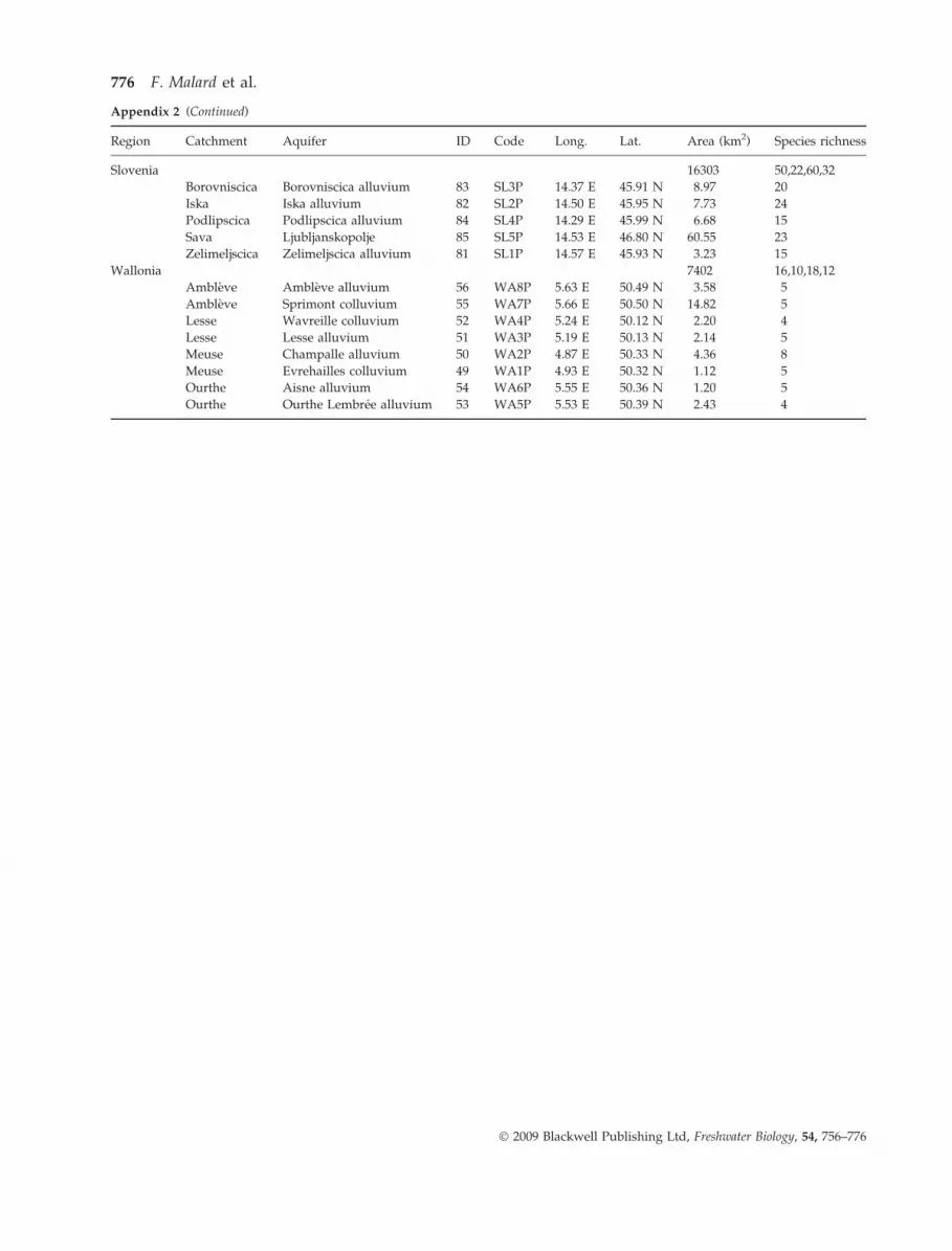
Appendix 2 (Continued)
Region Catchment Aquifer ID Code Long. Lat. Area (km2) Species richness
Slovenia 16303 50,22,60,32
Borovniscica Borovniscica alluvium 83 SL3P 14.37 E 45.91 N 8.97 20
Iska Iska alluvium 82 SL2P 14.50 E 45.95 N 7.73 24
Podlipscica Podlipscica alluvium 84 SL4P 14.29 E 45.99 N 6.68 15
Sava Ljubljanskopolje 85 SL5P 14.53 E 46.80 N 60.55 23
Zelimeljscica Zelimeljscica alluvium 81 SL1P 14.57 E 45.93 N 3.23 15
Wallonia 7402 16,10,18,12
Ambleve Ambleve alluvium 56 WA8P 5.63 E 50.49 N 3.58 5
Ambleve Sprimont colluvium 55 WA7P 5.66 E 50.50 N 14.82 5
Lesse Wavreille colluvium 52 WA4P 5.24 E 50.12 N 2.20 4
Lesse Lesse alluvium 51 WA3P 5.19 E 50.13 N 2.14 5
Meuse Champalle alluvium 50 WA2P 4.87 E 50.33 N 4.36 8
Meuse Evrehailles colluvium 49 WA1P 4.93 E 50.32 N 1.12 5
Ourthe Aisne alluvium 54 WA6P 5.55 E 50.36 N 1.20 5
Ourthe Ourthe Lembree alluvium 53 WA5P 5.53 E 50.39 N 2.43 4
776 F. Malard et al.
� 2009 Blackwell Publishing Ltd, Freshwater Biology, 54, 756–776