Advances in Water Resources 63 (2014) 152–166

Contents lists available at ScienceDirect

Advances in Water Resources

journal homepage: www.elsevier .com/ locate/advwatres

On temporal stochastic modeling of precipitation, nesting models acrossscales

0309-1708/$ - see front matter � 2013 Elsevier Ltd. All rights reserved.http://dx.doi.org/10.1016/j.advwatres.2013.11.006

⇑ Corresponding author.E-mail address: paschalis@ifu.baug.ethz.ch (A. Paschalis).

Athanasios Paschalis ⇑, Peter Molnar, Simone Fatichi, Paolo BurlandoInstitute of Environmental Engineering, ETH Zurich, Switzerland

a r t i c l e i n f o

Article history:Received 27 June 2013Received in revised form 19 November 2013Accepted 20 November 2013Available online 28 November 2013

Keywords:Stochastic rainfall modelsPoisson cluster modelMultiplicative Random CascadeMarkov chainAlternating renewal process

a b s t r a c t

We analyze the performance of composite stochastic models of temporal precipitation which can satis-factorily reproduce precipitation properties across a wide range of temporal scales. The rationale is that acombination of stochastic precipitation models which are most appropriate for specific limited temporalscales leads to better overall performance across a wider range of scales than single models alone. Weinvestigate different model combinations. For the coarse (daily) scale these are models based on Alternat-ing renewal processes, Markov chains, and Poisson cluster models, which are then combined with amicrocanonical Multiplicative Random Cascade model to disaggregate precipitation to finer (minute)scales. The composite models were tested on data at four sites in different climates. The results show thatmodel combinations improve the performance in key statistics such as probability distributions of pre-cipitation depth, autocorrelation structure, intermittency, reproduction of extremes, compared to singlemodels. At the same time they remain reasonably parsimonious. No model combination was found tooutperform the others at all sites and for all statistics, however we provide insight on the capabilitiesof specific model combinations. The results for the four different climates are similar, which suggests adegree of generality and wider applicability of the approach.

� 2013 Elsevier Ltd. All rights reserved.

1. Introduction

Stochastic simulation of precipitation time series at a site is de-manded for numerous applications where precipitation is a keyvariable, e.g., watershed hydrology, urban drainage design, naturalhazard assessment, agricultural and ecological applications, etc.These requirements have led to the formulation of many stochasticmodels of temporal precipitation. One of the fundamental prob-lems with existing models is that they are designed to perform bestwithin a limited range of time scales and for selected statistics forwhich they are calibrated. Often key statistics such as intermit-tency, correlation structure, extremes, etc., are not satisfactorilyreproduced at multiple scales. The premise behind this study isthat a simultaneous correct reproduction of key statistics over awide range of hydrologically relevant time scales from minutesto months is fundamental. We argue that even when simulatedprecipitation time series are to be used for instance for impactstudies at fine resolutions, we should require models at the sametime to provide good results at coarser resolutions, e.g., to preservestorm internal variability, intermittency and inter-storm clusteringproperties, seasonality, etc.

Early rainfall modeling focused on the simulation of daily pre-cipitation time series. The most common processes adopted inhydrology for stochastic simulation of precipitation were Markovchains [1–5], Alternating renewal processes [6,7] etc. Capabilitiesof such models have been recently enhanced using the conceptof generalized linear models (GLMs) (e.g., [8,9]). Those processesserved as precipitation simulation tools for some of the mostwidely used weather generators (e.g., [10,11]). A common defi-ciency of these models was that they were generally not able toreproduce higher order statistics and statistics across differenttemporal scales. Furthermore, they were not designed for temporalscales finer than daily, with some exceptions (e.g., [12]).

In order to improve precipitation simulations at fine resolutionsand for higher order statistics, new approaches were introduced.Among them point processes have been widely used [13,14]. Thesemodels appeared as an ideal candidate for precipitation modeling,since they reproduce a structure of storm arrivals and persistencethat mimics the physics of the precipitation process. Developmentson the initial ideas led to the implementation of Poisson clustermodels based on the concepts of storms, cells, and clustering[15–25]. Their main advantage was that statistics were reasonablyreproduced across scales from 1 h to several days, with the excep-tions of intermittency and correlation at high resolutions. Thesemodels have also been introduced into last generation weathergenerators (e.g., [26]) and used to solve practical problems in

A. Paschalis et al. / Advances in Water Resources 63 (2014) 152–166 153

real-world applications (e.g., [27]). Another class of models thatwas found to give promising results for rainfall simulation at var-ious temporal scales, even though often used for rainfall simulationat the daily scale only, is the Hidden Markov class of models (e.g.,[28–30]).

The concept of self similarity, widely known as fractal or scalingbehavior [31,32] combined with the quest for rainfall stochasticmodels that perform well across scales has led to an additional cat-egory of precipitation modeling. Self similarity has been identifiedin precipitation time series and precipitation spatial fields (e.g.,[33–36]). The concept of scale invariance has its origins in thestudy of turbulence [37,38] and it allows one to link statisticalproperties of a certain process (e.g., precipitation) across scales.The extension of the self similarity concept into multi-scalingbehavior, widely known as multifractals [39,40] has found manyinteresting applications in rainfall simulation (e.g., [41–44]). Oneof the modeling tools for the simulation of multifractals, Multipli-cative Random Cascades (MRC), has been widely used for precipi-tation disaggregation and downscaling [45–51].

Despite the large number of available approaches and modelsmentioned above, none is free of problems when multiple scalesand statistics are considered. Markov chains, Alternating renewalprocesses, and GLMs serve as reliable simulation tools for precipi-tation only for coarse aggregation scales and are often poor inreproducing extremes. Poisson cluster models have been foundto reproduce well the statistics only for the scales at which theyare calibrated (typically between one hour and a few days). Theself-similarity assumption and multifractal behavior have severallimitations, posing doubts on the generality and validity of the ap-proach. Temporal scaling regimes were found to be limited [52,53]and scaling relations themselves imperfect [54]. In the MRC it wasshown that weights do not follow iid (independent and identicallydistributed) assumptions required by the model [55,56], all ofwhich pose restrictions on the global scaling behavior ofprecipitation.

Significant effort has been undertaken to modify and improvethe original models. For example Katz and Parlange [12] applieda chain dependent process for hourly precipitation. Recently, Cow-pertwait et al. [57] introduced modifications to a Poisson clustermodel in order to overcome the common problem of inadequaterepresentation of small scale (sub-hourly) variability. Otherauthors provided several variants of the initial MRC model in orderto take into account dependencies of the MRC weights (e.g., onscale, rainfall intensity) [45,54,58–60]. However, these approacheshave the tendency to become increasingly difficult to parameter-ize. In summary, a single stochastic model which reproduces pre-cipitation statistics across a wide range of temporal scales ofhydrological interest is difficult to find.

An alternative approach which we explore in this study is tocombine several types of stochastic precipitation models at thescale for which they perform well. The nesting of an internal andexternal model is expected to strongly enhance the performanceof the precipitation generator across scales, without requiringexcessive parameterization if the nested models are appropriatelychosen. Although most studies in the literature have focused onimproving a specific model type, there are some attempts at modelcombinations. Menabde and Sivapalan [61] successfully applied acombination of an Alternating renewal process with a boundedMRC in order to reproduce rainfall extremes at fine temporalscales. Fatichi et al. [26] combined an autoregressive model witha Poisson cluster model to introduce into the latter the interannualvariability that it failed to capture. Veneziano and Iacobellis [62]obtained encouraging results combining an external model of con-ventional renewal type with an internal model based on the iter-ated random pulse process. Furthermore, Rodriguez-Iturbe et al.[15], Onof and Wheater [63] and Gyasi-Agyei and Willgoose [64]

improved the fine-scale properties of the Poisson cluster modelsby perturbing their realizations with an independent multiplica-tive noise stochastic process called jitter. Finally, Koutsoyiannis[65] developed a model-free theoretical framework in order tocouple different stochastic models.

The novelty in our work is to show that for stochastic modelingof temporal precipitation a composite model – consisting of apoint-process or Markov chain as an external model and a nestedMultiplicative Random Cascade as an internal model – performsbetter across a wider range of scales than the individual modelsalone and at the same time remains reasonably easy and parsimo-nious to calibrate. In order to make our point we extensively inves-tigate and compare different model types and structures for a widerange of statistics and temporal scales. We then apply the compos-ite models to four sites representing very different climatologicalregions around the world to verify their performance.

2. Data

Data from four meteorological stations with long records of reli-able high resolution precipitation were used. Each station belongsto a different climatological region of the world (Fig. 1 and Table 1).

Two of the stations are located in Europe. The first station, Zur-ich (Switzerland), is representative of a temperate continental cli-mate with distinct seasonality and a mean annual precipitation ofabout 1130 mm. The gauge has a heated tipping bucket recordingmechanism, and its temporal resolution is 10 min. Precipitationin Zurich mainly consists of stratiform events during the cold sea-son and intense convective events during the warm season [66].Data from this station have been used previously in several studies[45,56,67]. The second station, Florence (Italy), is representative ofa Mediterranean climate with a less pronounced seasonality, drysummers, and mean annual precipitation of about 800 mm. Thetipping bucket gauge in Florence records with a temporal resolu-tion of 5 min. Data from this station have also been extensivelyanalyzed in the past [68–70,62,71].

Outside of Europe we chose two stations with contrasting pre-cipitation regimes. Lucky Hills (Arizona, USA) is representative of asemiarid climate in southwestern USA. It is located within theAgricultural Research Service (ARS) Walnut Gulch ExperimentalWatershed [72]. Precipitation at Lucky Hills has a pronouncedseasonality with a wet monsoon season in the summer and rarestratiform events during the dry season. Mean annual precipitationis about 340 mm. The gauge is a weighing gauge with a temporalresolution of 1 min. Finally, the station Mount Cook (New Zealand)is representative of the oceanic climate of southern New Zealandwith a uniform distribution of precipitation throughout the year,accumulating an average of about 3900 mm per year. This highprecipitation total is the result of the orographic enhancementimposed by the southern Alps which leads to considerable precip-itation amounts in the entire southwestern area of New Zealand.The gauge is a tipping bucket with a temporal resolution of10 min. Data were obtained from the National Climatic Databaseoperated by NIWA (National Institute of Water and AtmosphericResearch).

Stronger diurnal patterns of precipitation intensity are onlypresent in the Mt. Cook and Lucky Hills stations (Fig. 1). These diur-nal patterns are mostly due to convective afternoon rain in thesummer, JJA for Lucky Hills and DJF for Mt. Cook.

3. Methods

The stochastic models which are used as building blocks for thecomposite model are presented in this section (Fig. 2). The compos-ite model consists of an external model which captures the

J FMAMJ J ASOND0

100

200

Dep

th [m

m]

Florence

JFMAMJ JASOND0

500

1000D

epth

[mm

]

Mt Cook

J FMAMJ J ASOND0

50

100

Dep

th [m

m]

Lucky Hills

J FMAMJ J ASOND0

100

200

Dep

th [m

m]

Zurich

0

0.2

0.4

0.6

Inte

nsity

[mm

h−1 ]

DJF

Lucky Hills Mt Cook Zurich Florence

MAM

0 5 10 15 200

0.2

0.4

Hour

JJA

0 5 10 15 20Hour

SON

Fig. 1. Locations of the stations and their seasonal mean diurnal cycle.

Table 1Analyzed precipitation stations in this study. H is station altitude, P is mean annual precipitation and Dt is the temporal resolution of the gauge.

Station Climate H (m) P (mm/yr) Dt (min) Data

Zurich (Switzerland) Temperate continental 556 1130 10 1981–2009Florence (Italy) Mediterranean 50 800 5 1962–1986Lucky Hills (Arizona, USA) Semi-arid 1372 340 1 1962–2012Mt Cook (New Zealand) Oceanic 765 3900 10 2000–2012

Fig. 2. Schematic representation of the composite model.

154 A. Paschalis et al. / Advances in Water Resources 63 (2014) 152–166

processes connected with storm arrivals (timing and intensity) andinter-storm periods. The finer time scales reached by the externalmodel are on the order of hours–days. The nested internal modelis then used to capture the processes which describe rainfall vari-ability within a storm by disaggregating the output of the externalmodel to finer time scales on the order of minutes.

Although the different combinations of external and internalmodels are calibrated independently at their appropriate timescales, the performance of the composite model is tested jointlyacross all simulated temporal scales. This means that the compos-ite model is used to simulate precipitation at the finest time scaleof interest and then simulated precipitation series are aggregatedback to any other chosen temporal scale, where relevant statisticsare computed and compared. The main statistical features weaim to reproduce at the different time scales are probability

distributions of precipitation depth, extreme event statistics,autocorrelation structure, and probability of zero precipitation.

One common assumption behind all the modeling combina-tions we used is the stationarity of the rainfall process. None ofthe models presented here can take into account the cyclostation-ary effect of the diurnal cycle. Although this is a limitation incertain cases, we are of the opinion that for the majority ofhydrological/agricultural/ecological applications, the effectsinduced by the daily cycle of precipitation can be considered small.For the cases where the diurnal pattern of precipitation isconsidered essential, different modeling techniques should be used(e.g., [12]).

3.1. External models

For the external model we used three approaches with differentlevels of complexity: the Alternating renewal process, Markovchain, and the Neyman Scott rectangular pulse model which be-longs to the so-called Poisson cluster model category.

3.1.1. Alternating renewal processThe Alternating renewal process (ARP) describes the precipita-

tion process as a sequence of wet and dry runs [73–75]. The dura-tions of the runs are assumed to follow a prescribed probabilitydistribution. The main assumption is that the wet and dry runsare independent, identically distributed (iid) and mutually inde-pendent. A constant intensity from a prescribed probability distri-bution is assigned to each day. These uniform intensities are alsoiid and independent of the duration of the wet run. Several distri-butions have been used in the literature and the choice is alwayssubjective and dependent on the analyzed dataset (e.g.,[73,74,76]). Here, we chose an exponential distribution for theduration of the dry and wet runs [7] and the two parameter gamma

A. Paschalis et al. / Advances in Water Resources 63 (2014) 152–166 155

distribution for precipitation intensity. The two parameter gammadistribution is a specific case of the generalized gamma distribu-tion which has been found to yield very good results for daily pre-cipitation depths worldwide [77]. However, we acknowledge thatdaily precipitation series possess heavy tails, a behavior whichthe two parameter gamma distribution cannot capture. When agood simulation of daily extremes is essential, potential candidatesfor the daily precipitation depths may include the Weibull, Paretodistribution, etc.

The ARP model has 4 parameters to be estimated (Table 2). Theestimation is based on the maximum likelihood method. Dry andwet spells and their respective daily depths are extracted fromthe rainfall records and their respective probability distributionsare fitted by maximizing their likelihood functions.

3.1.2. Markov chainThe Markov chain (MC) describes the precipitation occurrence

process in time through transition probabilities between wet anddry states. The two-state first order MC simulates a binary [0–1]process which corresponds to the dry (d) and wet (w) states withthe probability transition matrix,

M ¼pw;w pw;d

pd;w pd;d

!ð1Þ

where pi;j is the probability of transitioning from state i to state j inthe successive time step. A precipitation depth is assigned for eachtime step that the MC stays in the wet state. Precipitation depth isassumed iid and has a prescribed probability distribution, which wetake to be a two parameter gamma distribution identical to the ARP.

The probability transition matrix M is dependent on the se-lected time step of the MC model and has to be estimated fromdata at the same time scale. In this study the selected time stepwas approximately 1 day (1280 min). Equally, the distribution ofrainfall depth is related to this time step and has to be estimatedat the same time resolution. The fit of the rainfall depth distribu-tion was conducted by the maximum likelihood method [78]. Alto-gether the MC model has 4 parameters (Table 2), two parametersof the gamma distribution for rainfall depths and two parametersof the probability transition matrix pw;w and pd;d, which are relatedto the remaining probabilities pw;w þ pw;d ¼ 1 and pd;w þ pd;d ¼ 1.

Stochastic models based on the Markov chain process havebeen widely used in hydrology, especially for daily precipitation,due to their simplicity and parsimonious parametrization (e.g.,[4,79,?,80]).

Table 2Summary of model parameters.

Model Parameters Description

ExternalAlternating renewal process

(ARP)kw; kd Parameters of the exponential di

aARP ; bARP Gamma distribution parametersMarkov chain (MC) pw;w; pd;d Probability transition matrix term

aMC ; bMC Gamma distribution parametersNeyman Scott (NSRP) k; lc ; b; g; a; h Model parameters as described in

InternalMRC model A al; bl; ar; br Model parameters controlling the

scale and intensitya0; H Model parameters controlling the

MRC model B al; bl; ar; br Model parameters controlling thescale and intensity

a0; H; c0; c1; c2 Model parameters controlling theand intensity

3.1.3. Poisson cluster modelPoisson cluster models have gained popularity in hydrology

since they allow a more intuitive mechanistic description of theprecipitation process by including storms consisting of several cellswhich may superpose. Generally, Poisson cluster models can be di-vided into two different categories, the Neyman Scott rectangularpulse (NSRP) and the Bartlett Lewis rectangular pulse (BLRP)[81,23]. Both models simulate the precipitation process as a super-position of storms and rectangular rain cells with uniform intensityduring their lifetime. These models have significant similarities inthe clustering structure, however they differ in the way rain cellsare distributed in time. In the BLRP model, both the storm arrivalsand cell arrivals follow a Poisson process. In the NSRP model, stormarrivals also follow a Poisson process but within each storm a ran-dom number of cells is drawn and spaced out from the storm originaccording to a waiting time that has a specific probability distribu-tion. In both models cell depths and durations have prescribedprobability distributions.

For this work we chose the six parameter NSRP model [22].Even though several variants of the Poisson cluster models existwhich allow randomization of storm types, we chose the simpler6 parameter version of the model for two reasons: the parsimonyof the model structure, and because the efficiency of the Poissoncluster models with a more complex structure has been challenged(e.g., [81]). It was recently shown that the advantage of a Poissoncluster model with randomized storm parameters [27] was mini-mal when compared with the simpler 6 parameter NSRP modelused in this study [82].

Analytically the model is built as follows: (i) storms arrive as aPoisson process with rate k; (ii) each storm generates a number ofcells which follows a geometric distribution with mean value lc;(iii) the waiting time of cell origins after the origin of the storm fol-lows an exponential distribution with parameter b; (iv) the life-time (duration) of each cell follows an exponential distributionwith parameter g; (v) cell intensities follow a two parameter gam-ma distribution with scale and shape parameters a and h respec-tively (Table 2).

Parameter estimation is based on the numerical minimizationof an objective function which is the standardized mean square dif-ference between observed and analytically derived statistics [22].The statistics which are taken into account are mean, coefficientof variation, lag-one autocorrelation, probability of no rain, andthe conditional transition probabilities pd;d and pw;w. The modelwas calibrated at four time scales, i.e., T ¼ 1;6;24;72 h. Thenumerical minimization was conducted with a multi-startdownhill simplex algorithm similar to the approach of [24] for

stribution of the dry and wet spell durations

for the depth accumulationss

for the depth accumulationsCowpertwait [22]

dependence of the probability of zero of the MRC generator on the temporal

dependence of the a parameter of the Beta distribution on the temporal scale

dependence of the probability of zero of the MRC generator on the temporal

dependence of the a parameter of the Beta distribution on the temporal scale

10−1

100

101

102

10−6

10−5

10−4

10−3

10−2

10−1

depth (mm)

P(X

>x)

0.2 h21.3 hβ lognormalMRC B (microcanonical)

Fig. 3. Generated exceedance probabilities for the disaggregation of the daily timeseries for the Zurich station during spring (MAM), according to a canonical (b-lognormal) and a microcanonical (MRC B) model for the 10 min and the 1280 minaggregation interval. Markers correspond to observations and lines to simulatedseries.

156 A. Paschalis et al. / Advances in Water Resources 63 (2014) 152–166

the spatio-temporal version of the model. The analytical equationsof model statistics can be found in Cowpertwait et al. [21] andCowpertwait [22].

Even though the NSRP model is used at the (almost) daily timescale, we chose to also use finer temporal scales for its calibration.The reason is that some of the model parameters (i.e. duration ofthe rain cells) are mainly influenced by fine time scales e.g., hourly.Calibration of the NSRP model only at time scales coarser or equalthan daily would most likely provide much poorer results thanthose presented in this paper.

3.2. Internal models

The internal model which disaggregates the time series gener-ated by the external model down to the scale of the order of min-utes is based on a multiplicative redistribution of mass from coarseto fine scales – Multiplicative Random Cascade (MRC) model[39,40,83].

MRCs have been shown to be a very useful disaggregation/downscaling tool, especially for time scales ranging from one dayto few minutes [34,45,48,84]. The key parameter of a MRC is thecascade generator W which is a random variable that divides massfrom a single interval at one time scale into two intervals (in a dya-dic cascade with branching number b ¼ 2) in the next finer timescale. The precipitation depth at a scale n and time i in the cascadeis then,

RnðDinÞ ¼ R0

Yn

j¼1

WjðiÞ for i ¼ 1;2 . . . ; bn; ð2Þ

where R0 is the initial precipitation depth at the coarse scale. Thesubscript j represents the path of weights from R0 to RnðDi

nÞ.In this formulation the cascade generator W represents the frac-

tion of redistributed mass in every branching step. Since in ouranalysis we are interested in preserving mass exactly within theinternal model, we restrict the pair of W to sum up to 1 in everybranching step, which is known as the micro-canonical MRC. WhenW is not constrained at every branching step and is only requiredto have an expected value EðWÞ ¼ 1=b then we have a canonical(or macro-canonical) cascade which preserves mass on the average[59,85,86].

An additional reason to select the micro-canonical version ofthe MRC model is outlined below. To illustrate this, a disaggrega-tion of the ‘‘daily’’ (1280 min) precipitation time series for the Zur-ich station for the Spring season (MAM) is performed with amicrocanonical MRC model and a canonical MRC model and morespecifically the b-lognormal model [40,45,56] (Fig. 3). Although thecanonical b-lognormal model is capable of reproducing well theheavy tails of the fine scale (10 min) precipitation, aggregatingthe time series back to the original temporal scale (1280 min) dis-torts the distribution of the depths. This is because the aggregatedseries at the 1280 min temporal scale corresponds to the so-calleddressed quantities [31], and its distribution is distorted due to thedistribution of the dressing factor. Further investigations on this is-sue are beyond the scope of this study, but the interested readercan refer to (e.g., [31,87–89] and references therein).

Because precipitation is an intermittent process, it is furthernecessary to introduce the probability that the cascade generatorW ¼ 0,

PðWðiÞ ¼ 0 or Wðiþ 1Þ ¼ 0Þ ¼ p0; ð3Þ

where i; iþ 1 correspond to an arbitrary pair of complementaryweights in the cascade development with branching number b ¼ 2.

In order to achieve mass conservation, the positive part of thegenerator Wþ, has to be bounded in ½0;1�. Here, we assumed thatthe positive part of the generator can be described by a single

parameter (symmetric) Beta distribution with probability distribu-tion function (pdf),

f ðWþÞ ¼ 1Bða;aÞW

þa�1ð1�WþÞa�1; ð4Þ

where Bða;aÞ is the Beta function and a is a parameter related to thevariance of W (e.g., [45]). The estimation of the a parameter of theBeta distribution was carried out using the method of moments,

a ¼ 18VarðWþÞ

� 0:5; ð5Þ

where Wþ values were estimated from the data as the ratio be-tween precipitation depths at two successive (embedded) temporalscales, if both precipitation depths are positive and not equal (i.e.0 < Wþ < 1).

In the original formulation of the MRC it is assumed that thecascade generator W is independent and identically distributed(iid) across the entire range of scales. However, it has been shownthat the probability distribution of W, in both its parts f ðWþÞ andp0, is dependent on the aggregation scale of the precipitation pro-cess [45,61]. Paschalis et al. [56] following the ideas of Cârsteanuand Foufoula-Georgiou [55] identified a temporal dependencestructure in W using a large dataset in Switzerland. Dependenciesof the parameters of the cascade generator (in a canonical MRC)with the mean intensity of the process were also identified [54].Consequently, these relations were included in recent variants ofthe MRC models (both canonical and micro-canonical) to betterfit the precipitation statistics across temporal scales from minutesto days [59,60].

To explore the effect of scale dependence we used two variantsof the micro-canonical MRC model parameterized by Rupp et al.[59]. Models with lower complexity, even though they are moreparsimonious and thus more attractive, yielded substantiallyworse results and are not reported here.

3.2.1. MRC model AIn the MRC model A, p0 is dependent on the temporal aggrega-

tion scale and on the average intensity of precipitation at the next

A. Paschalis et al. / Advances in Water Resources 63 (2014) 152–166 157

(coarser) aggregation scale. The parameter a of the Beta distribu-tion of Wþ is dependent only on the temporal aggregation scale.

The probability of a non-zero weight at the cascade develop-ment is parameterized as [59]

PxðI; sÞ ¼ 1� p0ðI; sÞ ¼12

1þ erflogðIÞ � lffiffiffi

2p

r

� �� �; ð6Þ

where s is the temporal scale of the cascade, I is the precipitationintensity of the coarser scale, and erf is the error function definedas erfðxÞ ¼ 2ffiffiffi

ppR x

0 e�t2 . The parameters l and r depend linearly onthe logarithm of the temporal scale of the cascade,

l ¼ al logðsÞ þ bl; ð7Þ

r ¼ ar logðsÞ þ br: ð8Þ

The parameter of the Beta distribution is only dependent on thetemporal scale, s,

aðsÞ ¼ a0sH: ð9Þ

The model has 6 parameters which were estimated for all thestations for temporal scales from 10 min to approximately 1 day(Table2). The estimation of the parameters was carried out usingleast square fitting for the Eqs. (6)–(9).

3.2.2. MRC model BIn the MRC model B both p0 and the parameter a of the Beta dis-

tribution are dependent on the temporal aggregation scale andaverage intensity of precipitation at the next (coarser) aggregationscale [59].

The parametrization of the probability of non-zero weights inthe cascade is as in Eq. (6). The a parameter of the Beta distributionis conditioned both on the temporal scale and precipitation inten-sity at the coarser scale,

log½a�ðIÞ� ¼ c0 þ c1 logðIÞ þ c2½logðIÞ�2; ð10Þ

and

aðI; sÞ ¼ a�ðIÞa0sH: ð11Þ

The estimation of the polynomial coefficients ci for lower inten-sities (typically <1 mm h�1) can be problematic due to precisionartifacts introduced by the tipping mechanism of the gauges. Forthis reason, the fitting procedure of Eq. (10) was restricted to tem-poral scales coarser than 20 min. In some cases the second orderpolynomial introduced in Eq. (11) could be simplified to a first or-der polynomial or even to a constant, however the above parame-trization is kept for consistency with Rupp et al. [59].

The model has 9 parameters which were estimated for all thestations for temporal scales from 10 min to approximately 1 day(Table 2). Similarly to MRC model A, the estimation of the param-eters was carried out using least square fitting for the Eqs. (6)–(8),(10) and (11).

3.3. Temporal scales and validation statistics

The time scale at which we combine the external and internalmodels is derived from results of previous research and from ourown analyses which show that the ARP and MC models (at leastin their most parsimonious form used in this study, see [12] foran exception) are most appropriate for temporal scales up to1 day. The NSRP model can produce reliable results for scales downto one hour, especially when calibrated at sub-daily scales (e.g.,[26,23]), which could be another possible temporal scale of nestingfor the NSRP model. However, recent findings using spectral anal-ysis for a number of stations in Switzerland [90,91] suggest thatthe (spatio-temporal) NSRP model fails to capture adequately the

small scales of precipitation (<10 h). These results, supported byour current findings, suggest that nesting a Poisson cluster modelat the hourly time scale with a MRC could be less optimal thannesting at the daily scale. At the same time previous studies haveshown that MRC models are particularly suitable for scales from1 day to a few minutes [45,54,92]. Based on these considerationsand on a branching number b ¼ 2 for the MRC model, we decidedto use the external models to simulate continuous precipitationtime series at time scales T ¼ 1280 min (21.3 h) and the internalMRC models disaggregate these from T ¼ 1280 down toT ¼ 10 min. The time scale of the temporal nesting has to be thesame for all the combinations, in order to achieve a fair compari-son. A summary of parameters of all models can be found inTable 2.

In order to take into account diverse precipitation triggeringmechanisms during the year and ensure as far as possiblestationarity of the precipitation record, the analysis for all of thestations was conducted on a seasonal basis. A sample of 50realizations for a 10-year period with temporal resolution 10 minwas simulated for all stations. While some of the results areanalyzed across a wide range of temporal scales, the comparisonamong composite models is assessed at three specific temporalscales.

The highest resolution T ¼ 10 min (�0.2 h) roughly matches thetime scale at which most of the records were collected (see Ta-ble 1). Rainfall variability at such fine resolutions can be crucialfor many applications, for example analyzing the response of urbancatchments or steep mountain basins with very low runoff concen-tration times that are usually prone to flash floods. The second timescale is T ¼ 160 min (2.7 h) which corresponds roughly to themean duration of high intensity convective storms. The third timescale is T ¼ 1280 min (21.3 h) which is the temporal scale at whichwe combined the external and internal models, and which is rep-resentative of stratiform precipitation events. At this time scalewe only validate the performance of the external stochastic model.It should be noted that in our analysis we consider the observedprecipitation time series as a realization of a stationary process,on a seasonal basis. The reason for this choice is to have a fair com-parison with the output of the models which are as well realiza-tions of stationary processes. In case of nonstationarities, such asa strong diurnal pattern, biases on the estimated statistics can oc-cur (e.g., apparent autocorrelations, higher skewness due to thedaily cycle, etc.).

The efficiency of each model combination was validated for itsability to reproduce the probability distributions of precipitationdepth at different temporal scales, extremes, autocorrelation struc-ture, and probability of zero precipitation.

4. Results

4.1. NSRP as a benchmark

We first present results of the Poisson cluster model alone as abenchmark for the results obtained by the composite models. TheNSRP model is chosen as a benchmark since it is the only modelpresented here that has been widely used as a ‘‘multi-scale’’ simu-lation tool. The other external models, at least in their most parsi-monious form, are not capable of reproducing fine scale temporalstatistics (less than daily).

In Fig. 4 the performance of the NSRP model is summarized forthe Zurich station. In general the model efficiency in reproducingprecipitation statistics for temporal scales coarser than hourly isexcellent, however significant departures are found for the sub-hourly scale. Due to the simplified representation of the precipita-tion process as a superposition of rectangular rain cells, small-scale

10−1

100

101

102

10−6

10−4

10−2

100

depth (mm)

P(X

>x)

0.2 h2.7 h21.3 h85.3 h213.3 h

0 5 10 15 20−0.2

0

0.2

0.4

0.6

0.8

lag

AC

F

0.2 h2.7 h21.3 h

50 100 1500

0.2

0.4

0.6

0.8

1

aggregation interval [h]

P(r

=0)

ObservedModelled

100

102

104

10−4

10−3

10−2

10−1

100

Time [h]

P(X

>x)

Wet durations

0.2 h2.7 h21.3 h85.3 h213.3 h

(a) (b)

(c) (d)

Fig. 4. Simulated statistics for the Neyman Scott model for spring season (MAM) for the Zurich station. Markers represent observations and lines the mean simulated values.(a) Exceedance probabilities of precipitation depth accumulated at different temporal scales. (b) Autocorrelograms with 90% confidence bounds on the simulations. (c)Probabilities of zero precipitation with 90% confidence bounds on the simulations shaded. (d) Exceedance probabilities of the wet spell durations for different aggregationintervals.

Fig. 5. Power spectrum for the simulated Neyman Scott model for spring season(MAM) for the Zurich station. The dashed line is the mean spectrum of thesimulated realizations shown by thin gray lines.

158 A. Paschalis et al. / Advances in Water Resources 63 (2014) 152–166

variability cannot be simulated. The finest temporal scale offluctuations is associated with the distribution of the rain celllifetime that is typically not short enough in the model to properlycharacterize the true precipitation process at this scale.

The simulated precipitation time series severely underestimatethe occurrence of 10-min rainfall depths greater than 1 mm(Fig. 4(a)). The simulated series are very smooth at this temporalscale, leading to very high autocorrelations (Fig. 4(b)). Another typ-ical problem that is associated with the NSRP model is its inabilityto successfully reproduce the probability of zero precipitation (e.g.,[18]). In our example, the probability of no rain is slightly overes-timated for large scales of aggregation (Fig. 4(c)), even though it isone of the statistics that are explicitly considered in the calibrationprocedure.

Intermittency is connected to wet and dry spell durationsthrough clustering of the precipitation process. As a wet periodwe define here the duration for which precipitation accumulatedat the selected temporal resolution stays continuously above zero.This notation is somewhat different from the definition of stormduration (e.g., [93]). The distribution of wet spell durations at thestudied temporal aggregation scales is shown in Fig. 4(d). Similarlyto the other statistics, the performance for time scales above 1 h isvery good, however for the 10-min scale there is a significant over-estimation of short wet spell durations by the model. The NSRPmodel is not able to adequately generate gaps within storms andshort rainfall pulses for structural reasons, despite the fact thatthe transition probabilities from dry to wet states were also takeninto account in the calibration procedure.

The correlation structure across temporal scales was also exam-ined with spectral analysis. Fig. 5 shows the observed and simu-lated power spectra for the Zurich station. The strongautocorrelation at high temporal resolutions in the model results

A. Paschalis et al. / Advances in Water Resources 63 (2014) 152–166 159

in a steeper spectral decay for higher frequencies. The divergencebetween observed and simulated series starts roughly at temporalscales of about 5 h, which could be considered a reasonable scalefor nesting NSRP with other stochastic models. In summary theNSRP model alone as a benchmark performs very well for scalesabove 1 h, but not for scales below 1 h. In the next step we inves-tigate if and how different composite models improve the high res-olution performance.

4.2. Composite model results

Different composite model combinations are evaluated for thesame statistics analyzed for the NSRP model. The combinationswe show are Markov chain–MRC model B (Fig. 6), Neymann–ScottNSRP–MRC model B (Fig. 7) and the Alternating renewal processmodel–MRC model B (Fig. 8). Combinations of the external modelswith MRC model A, gave systematically worse results and are dis-cussed only in the model and station intercomparison Section 4.3.We recall that the behavior of the composite models at temporalscales greater than 1 day is solely dependent on the external modelwhile the behavior at finer temporal scales depends on both theexternal and the internal model.

One of the most important improvements, and common to allthe composite models, is a substantial enhancement in the repro-duction of the probability distribution for the high resolution pre-cipitation depths. Another common feature to all of the models isthe improvement in the representation of the probability of zeroprecipitation. The combination that uses the NSRP model as the

10−1

100

101

102

10−6

10−5

10−4

10−3

10−2

10−1

100

depth (mm)

P(X

>x)

0.2 h2.7 h21.3 h85.3 h213.3 h

50 100 1500

0.2

0.4

0.6

0.8

1

aggregation interval [h]

P(r

=0)

ObservedModelled

(a)

(c) (d

Fig. 6. Simulated statistics for the combination of Markov chain and MRC model

external model performs worse than the others for this statistic,since errors at scales coarser than 1 day cannot be improved upon.Nevertheless, the performance is improved with respect to NSRPalone. The probability distributions of the wet spell durations aresignificantly better represented at small scales even though, in allof the cases, there is a systematic underestimation of the tails forthe 10-min aggregation interval. This means that the compositemodels fall short in capturing long wet spells observed at thisresolution.

The positive effect of the MRC models at temporal resolutionsbelow 1 day is evident. Overall, the performance is better at the10-min resolution than at coarser aggregations. For example,the autocorrelations at intermediate scales of a few hours are notperfectly reproduced. Even though they are almost perfect at the10-min scale. The underlying reason can be found in the parameter-izations of the microcanonical MRCs that are not always sufficient tocapture the entire variability/correlation of rainfall. In this case, hea-vier parameterizations could improve the simulations, but would goagainst the philosophy of a parsimonious and generic model.

Generally, the performance at high resolutions increases withthe MRC model complexity. As shown in Fig. 9 the reproductionof the tail of the distribution is much better when the MRC modelB is used. This is also reflected in the better reproduction of the an-nual extremes (Fig. 10). For all the other statistics, both versions ofthe MRC model (A & B) comparably improve the performance withrespect to the NSRP model.

In terms of statistics at temporal scales greater than 1 day, themore complex the external model is, the better it performs. The

0 5 10 15 20−0.2

0

0.2

0.4

0.6

0.8

lag

AC

F

0.2 h2.7 h21.3 h

100

102

104

10−4

10−3

10−2

10−1

100

Time [h]

P(X

>x)

Wet durations

0.2 h2.7 h21.3 h85.3 h213.3 h

(b)

)

B for spring season (MAM) for the Zurich station. Notation same as in Fig. 4.

10−1

100

101

102

10−6

10−5

10−4

10−3

10−2

10−1

100

depth (mm)

P(X

>x)

0.2 h2.7 h21.3 h85.3 h213.3 h

5 10 15 20−0.2

0

0.2

0.4

0.6

0.8

1

lag

AC

F

0.2 h2.7 h21.3 h

50 100 1500

0.2

0.4

0.6

0.8

1

aggregation interval [h]

P(r

=0)

ObservedModelled

100

102

104

10−4

10−3

10−2

10−1

100

Time [h]

P(X

>x)

Wet durations

0.2 h2.7 h21.3 h85.3 h213.3 h

(a) (b)

(c) (d)

Fig. 7. Simulated statistics for the combination of the Neyman Scott and MRC model B for spring season (MAM) for the Zurich station. Notation same as in Fig. 4.

160 A. Paschalis et al. / Advances in Water Resources 63 (2014) 152–166

results of the composite models based on the NSRP model (Fig. 7)are typically better than the performance of the model based onAlternating renewal processes and Markov chains (Figs. 8 and 6).Common problems associated with the latter models are the sys-tematic underestimation of the tail of the distribution of accumu-lation depths for temporal scales beyond one day. Some of thoseproblems could have been solved using more complex distribu-tions of daily depths [77,94]. However, this would have also in-creased the parameterization of the models. Furthermore, thechoice of the distribution could become station-dependent limitingits generality.

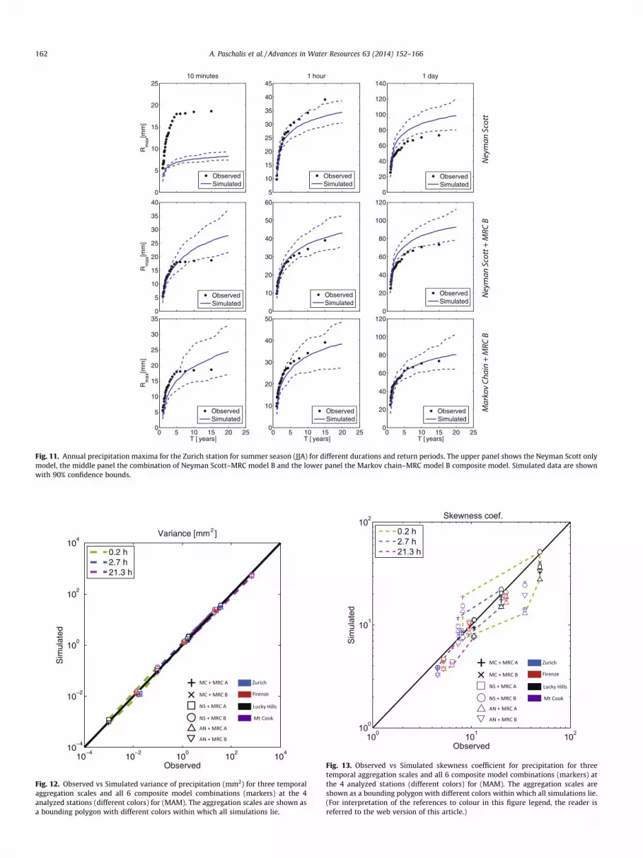
An important statistical property which stochastic precipitationmodels should be able to reproduce are extremes. A critical test formodels is their ability to capture the depth-duration-frequencyrelationships for annual maxima. These are shown for durationsD ¼10 min, 1 h and 1 day for the NSRP Model only, the combina-tion of NSRP–MRC model B and the Markov chain–MRC model Bcombination in Fig. 11. The performance of the composite modelis very good for all three durations, and significantly improvesthe single NSRP model which underestimates the extremes at the10-min scale and overestimates the daily maxima. The excellentperformance of the composite model is not a trivial result becauseannual maxima for short durations are determined by the indepen-dent behavior of both the external and internal models.

4.3. Model and station inter-comparison

After the illustrative presentation of the various model combi-nations for the Zurich station, we seek a model and station inter-comparison and synthesis in this section. The questions raised

are (i) if all composite models perform equally well; and (ii) if thisperformance is dependent on the station itself. The overall goal isto identify the general patterns of the efficiency of each modelcombination that may serve as a selection criterion.

We chose 4 basic statistics to illustrate model performance:variance (Fig. 12), skewness (Fig. 13), probability of no rain(Fig. 14) and lag-one autocorrelation (Fig. 15). The statistics in eachfigure are estimated at three temporal aggregation scales (10-min,2.7 h and 21.3 h), for all 6 composite model combinations at allfour stations. The three temporal aggregation scales are shown asa bounding polygon within which all simulations lie. The analysiswas conducted on a seasonal basis, and the results we show arefor Spring (MAM) only, which in terms of performance was anaverage season. Results for the other seasons are similar and theydo not affect the conclusions of this study [82].

First of all, the mean value was almost perfectly preserved forall the modeling approaches, and thus is not shown here. The var-iance (Fig. 12) is practically perfectly reproduced by all compositemodels, at all stations and temporal scales because it is used di-rectly or indirectly in the calibration of both external and internalmodels.

Larger differences are evident in the asymmetry of the precipi-tation distributions measured by the skewness coefficient (Fig. 13).Generally, the efficiency of all models is relatively good. The scatteraround the perfect agreement line reveals some of the commonfeatures between all the models. For all the stations the ability ofthe combination that employs the MRC model B as the disaggrega-tion model performs better than the equivalent combination thatuses the MRC model A. This is a strong indication that a parametri-zation of the cascade generator dependent both on the temporal

10−1

100

101

102

10−6

10−5

10−4

10−3

10−2

10−1

100

depth (mm)

P(X

>x)

0.2 h2.7 h21.3 h85.3 h213.3 h

0 5 10 15 20−0.2

0

0.2

0.4

0.6

0.8

lag

AC

F

0.2 h2.7 h21.3 h

50 100 1500

0.2

0.4

0.6

0.8

1

aggregation interval [h]

P(r

=0)

ObservedModelled

100

102

104

10−4

10−3

10−2

10−1

100

Time [h]

P(X

>x)

Wet durations

0.2 h2.7 h21.3 h85.3 h213.3 h

(a) (b)

(c) (d)

Fig. 8. Simulated statistics for the combination of the Alternating renewal process and MRC model B for spring season (MAM) for the Zurich station. Notation same as in Fig. 4.

5 10 1510

−6

10−4

10−2

depth (mm)

P(X

>x)

ObservedNeyman−ScottNeyman−Scott + MRC ANeyman−Scott + MRC B

Fig. 9. Simulated exceedance probabilities for the precipitation depth at the 10 minaggregation interval according to the Neyman Scott model and its combination withthe MRC model A and MRC model B.

1 1052 200

5

10

15

20

25

30

T [years]

Rm

ax[m

m]

ObservedNSNS + MRC ANS + MRC B

Fig. 10. Generated annual maxima for the 10 min aggregation interval according tothe Neyman Scott model and its combination with the MRC model A and MRCmodel B.

A. Paschalis et al. / Advances in Water Resources 63 (2014) 152–166 161

scale and the precipitation intensity is an improvement. Nosignificant differences between the various stations could be fur-ther identified, also because of the sensitivity of the coefficient ofskewness to outliers.

The probability of zero precipitation is well reproduced by allmodels although patterns can be identified (Fig. 14). The combina-tion of Markov chain and any MRC model give almost perfectresults for all the analyzed temporal scales and stations. The

combinations of NSRP and MRC models, in most of the aggregationintervals overestimate slightly the probability of no rainfall. Theoverestimation of the zero probability associated with the use ofthe NSRP model [18,16,95] is expected to be higher for aggregationintervals larger than 1 day. The combination of the ARP and MRCmodels gives exactly the opposite result, systematically underesti-mating the probability of zero precipitation. The reason is that theexponential distribution that was selected for parametrizing drydurations does not capture well the tails of the dry periods. A selec-tion of a more heavy tailed distribution would yield better results,but at the same time increase the number of parameters. For the

0

5

10

15

20

25

Rm

ax[m

m]

10 minutes

ObservedSimulated

5

10

15

20

25

30

35

40

451 hour

ObservedSimulated

0

20

40

60

80

100

120

1401 day

ObservedSimulated

0

5

10

15

20

25

30

35

40

Rm

ax[m

m]

ObservedSimulated

0

10

20

30

40

50

60

ObservedSimulated

0

20

40

60

80

100

120

ObservedSimulated

0 5 10 15 20 250

5

10

15

20

25

30

35

T [ years]

Rm

ax[m

m]

ObservedSimulated

0 5 10 15 20 250

10

20

30

40

50

T [ years]

ObservedSimulated

0 5 10 15 20 250

20

40

60

80

100

120

T [ years]

ObservedSimulated

Fig. 11. Annual precipitation maxima for the Zurich station for summer season (JJA) for different durations and return periods. The upper panel shows the Neyman Scott onlymodel, the middle panel the combination of Neyman Scott–MRC model B and the lower panel the Markov chain–MRC model B composite model. Simulated data are shownwith 90% confidence bounds.

10−4

10−2

100

102

104

10−4

10−2

100

102

104

Observed

Sim

ulat

ed

0.2 h2.7 h21.3 h

Variance [mm ]

+ ×

MC + MRC A

MC + MRC B

NS + MRC A

NS + MRC B

AN + MRC A

AN + MRC B

Zurich

Firenze

Lucky Hills

Mt Cook

2

Fig. 12. Observed vs Simulated variance of precipitation (mm2) for three temporalaggregation scales and all 6 composite model combinations (markers) at the 4analyzed stations (different colors) for (MAM). The aggregation scales are shown asa bounding polygon with different colors within which all simulations lie.

100 101 102100

101

102

Observed

Sim

ulat

ed

0.2 h2.7 h21.3 h

Skewness coef.

+ ×

MC + MRC A

MC + MRC B

NS + MRC A

NS + MRC B

AN + MRC A

AN + MRC B

Zurich

Firenze

Lucky Hills

Mt Cook

Fig. 13. Observed vs Simulated skewness coefficient for precipitation for threetemporal aggregation scales and all 6 composite model combinations (markers) atthe 4 analyzed stations (different colors) for (MAM). The aggregation scales areshown as a bounding polygon with different colors within which all simulations lie.(For interpretation of the references to colour in this figure legend, the reader isreferred to the web version of this article.)

162 A. Paschalis et al. / Advances in Water Resources 63 (2014) 152–166

0.5 0.6 0.7 0.8 0.9 10.5

0.55

0.6

0.65

0.7

0.75

0.8

0.85

0.9

0.95

1

Observed

Sim

ulat

ed

0.2 h2.7 h21.3 h

Probability of zero precipitation [-]

Fig. 14. Observed vs Simulated probability of zero rainfall for three temporalaggregation scales and all 6 composite model combinations (markers) at the 4analyzed stations (different colors) for (MAM). The aggregation scales are shown asa bounding polygon with different colors within which all simulations lie. (Forinterpretation of the references to colour in this figure legend, the reader is referredto the web version of this article.)

0 0.2 0.4 0.6 0.8 10

0.1

0.2

0.3

0.4

0.5

0.6

0.7

0.8

0.9

1

Observed

Sim

ulat

ed

0.2 h2.7 h21.3 h

Lag 1 autocorrelation coef [-]

Fig. 15. Observed vs Simulated lag-one autocorrelation coefficient for threetemporal aggregation scales and all 6 composite model combinations (markers)at the 4 analyzed stations (different colors) for (MAM). The aggregation scales areshown as a bounding polygon with different colors within which all simulations lie.(For interpretation of the references to colour in this figure legend, the reader isreferred to the web version of this article.)

A. Paschalis et al. / Advances in Water Resources 63 (2014) 152–166 163

highest resolution scale, the largest discrepancies in the probabilityof no rain was found for the wettest station (Mt Cook). For thisdataset the parameterization of the probability of zero rain p0 inthe MRC models with intensity and scale (Eq. 6) was notsatisfactory.

A correct representation of the autocorrelation function is crit-ical for all composite models. We present only the lag-one autocor-

relation coefficient (Fig. 15). At the daily scale, where we canvalidate the performance of the external models, the NSRP modeloutperforms the other two models for all the stations. Moreover,at Mt. Cook the performance is overall not good at this scale forany model. The Markov chain and the Alternating renewal processsystematically underestimate the autocorrelation function due tothe assumption of the iid daily rainfall depths. Another optionwe explored but not reported here, was to assume a uniform inten-sity across the wet spells for the ARP model. Such an option led to asubstantial overestimation of the autocorrelation for the dailyscale. At the intermediate scale (2.7 h) all the model combinationsunderestimate the lag-one correlation coefficient. The underesti-mation is more dependent on the station rather than on the model.For the highest resolution (10-min) the models do reasonably well,with a tendency to a slight underestimation which is also stationdependent.

Overall the largest differences in the reproduction of the lag-one correlation between models is found at Mt. Cook. This is theonly station with a notable difference between the internal disag-gregation models MRC A and B for this statistic. In all cases, MRCmodel B outperforms MRC model A.

Despite the large uncertainty of the results, due to the limitednumber of stations that are used in this study, we provide somegeneral guidelines for the model selection. Regarding the MRCmodels, it was found that a parametrization that introduces depen-dencies of the distribution of the cascade generator W in both scaleand intensity is needed. Various parametric forms of such relation-ships can be found in the literature (e.g., [54,59,60]), and mostprobably the optimal choice will depend on the analyzed station.The choice of the external model should be driven by the specificapplication for which precipitation is simulated. For instance, MCmodels lead to a better representation of the probability of precip-itation occurrence, and may be preferable in drought or water re-sources management studies. The NSRP model represents betterthe correlation properties of precipitation, and may be preferablefor flood risk analyses.

Since data from only 4 stations have been used, any generaliza-tion on the applicability of each model combination would be pre-mature. Future analysis on more extensive datasets will potentiallyreveal if an optimal model combination exists for differentclimates.

5. Discussion and conclusions

The topic of this study was to compare and combine methodsfor stochastic modeling of precipitation time series. We set out toovercome common problems of the most widely used stochasticprecipitation models and propose an alternative strategy for mod-eling temporal precipitation. The methodology that is presentedhere is to combine different stochastic models across the rangeof temporal scales where they perform best.

Traditional modeling techniques, even if they are developed inorder to reproduce multi-scale statistics, such as Poisson clustermodels and Multiplicative Random Cascades, suffer from seriousrestrictions. Inherent structural problems in these models do notallow robust simulation across a wide range of scales. Combiningdifferent techniques at temporal scales where they have beenfound to perform well can enhance the applicability of a modelwith a minor increase in the number of parameters.

We examined six different model combinations in this study.All of them consisted of two stochastic models – an external modelfor coarse scales (Alternating renewal process, Markov chain, Pois-son cluster model of the Neyman Scott type) and an internal disag-gregation model for fine scales (two versions of the microcanonicalMultiplicative Random Cascade). The composite models were

164 A. Paschalis et al. / Advances in Water Resources 63 (2014) 152–166

tested on high resolution precipitation data at four sites in differ-ent climates.

As a first result we showed that the NSRP model by itself wasnot able to reproduce satisfactorily statistics at the highest(10-min) resolution, in particular, the tails of the rainfall depthdistributions, the probability of no rain, wet/dry spell durationsand serial correlation structure. Adding a MRC model to disaggre-gate simulated precipitation from the daily scale vastly improvedthese statistics. Good performance at the 10-min scale was alsoshown for the other composite models. The added value of thenested internal model was most evident in the analysis ofextremes for different durations, where for example we showedthat the MC-MRC-B combination reproduced almost perfectly thedepth-duration-frequency relations for different aggregationtimes, while the NSRP model alone had significant bias fordurations (time scales) which were not used in its calibration.

Second, the results do not give clear evidence for which com-posite model is best overall. Each of the model combinations hasits own advantages, mainly based on the properties of the externalmodel that influence the fine scale statistics through the MRC. Forinstance the MC-MRC model combinations were best for repre-senting intermittency at all scales, while the NSRP-MRC modelswere on the average best for autocorrelation. The choice of theappropriate modeling approach should be based on the most sig-nificant statistics that need to be preserved in the application.The most evident result of the comparison was between the twovariants of the MRC models. For all the stations, the more complexstructure of the MRC model systematically provided better results.Therefore, dependence of the cascade weights both on scale andintensity was found to be significant for all the climates.

Third, autocorrelation is difficult to reproduce across all rele-vant scales. At the minute to hourly temporal aggregation scaleslag-one autocorrelation was underestimated by practically allmodel combinations at all stations. This suggests a problem withthe discrete MRC which does not reproduce the autocorrelationstructure of rainfall accurately. To overcome this issue, differentdisaggregation procedures can be tested as alternative options infuture research. However, the fact that the composite models per-form reasonably well for stations from such different climatesstrengthens the argument that the proposed methodology has gen-eral validity and potentially wide applicability.

Acknowledgments

We would like to thank the anonymous referees and the editor,Andrea Rinaldo, for their helpful comments that improved themanuscript. Precipitation data for Switzerland were provided byMeteoSwiss, the Federal Office of Meteorology and Climatology.Funding for this research was provided by the Swiss NationalScience Foundation Grant 20021-120310.

References

[1] Todorovic P, Yevjevich V. Stochastic process of precipitation. Technical report,Colo. State Univ. Fort Collins, Fort Collins, Colorado; 1969.

[2] Todorovic P, Woolhiser DA. A stochastic model of n-day precipitation. J ApplMeteorol 1975;14:17–24. http://dx.doi.org/10.1175/1520-0450(1975)014<0017:ASMODP>2.0.CO;2.

[3] Chin E. Modeling daily precipitation occurrence process with Markov chain.Water Resour Res 1977;13:949–56. http://dx.doi.org/10.1029/WR013i006p00949.

[4] Katz R. Precipitation as a chain-dependent process. J Appl Meteorol1977;16:671–6. http://dx.doi.org/10.1175/1520-0450(1977)016<0671:PAACDP>2.0.CO;2.

[5] Foufoula-Georgiou E, Lettenmaier D. A Markov renewal model for rainfalloccurrences. Water Resour Res 1987;23:875–84. http://dx.doi.org/10.1029/WR023i005p00875.

[6] Schmitt F, Vannitsem S, Barbosa A. Modeling of rainfall time series using two-state renewal processes and multifractals. J Geophys Res 1998;103:23,181–93.http://dx.doi.org/10.1029/98JD02071.

[7] Ivanov VY, Bras RL, Curtis DC. A weather generator for hydrological, ecological,and agricultural applications. Water Resour Res 2007;43. http://dx.doi.org/10.1029/2006WR005364.

[8] Yang C, Chandler RE, Isham VS, Wheater HS. Spatial-temporal rainfallsimulation using generalized linear models. Water Resour Res 2005;41.http://dx.doi.org/10.1029/2004WR003739.

[9] Chandler RE, Wheater HS. Analysis of rainfall variability using generalizedlinear models: a case study from the west of Ireland. Water Resour Res2002;38. http://dx.doi.org/10.1029/2001WR000906.

[10] Richardson C. Stochastic simulation of daily precipitation, temperature, andsolar radiation. Water Resour Res 1981;17:182–90. http://dx.doi.org/10.1029/WR017i001p00182.

[11] Racsko P, Szeidl L, Semenov M. A serial approach to local stochastic weathermodels. Ecol Model 1991;57:27–41. http://dx.doi.org/10.1016/0304-3800(91)90053-4.

[12] Katz R, Parlange M. Generalizations of chain-dependent processes: applicationto hourly precipitation. Water Resour Res 1995;31:1331–41. http://dx.doi.org/10.1029/94WR03152.

[13] Le Cam L. A stochastic description of precipitation. In: Neyman J, editor.Proceedings of fourth berkeley symposium on mathematical statistics andprobability, vol. 3. Berkeley: Univ. of Calif. Press; 1961. p. 165–76.

[14] Cox D, Isham V. A simple spatial-temporal model of rainfall. Proc R Soc LondSer A Math Phys Sci 1988;415:317–28. http://dx.doi.org/10.1098/rspa.1988.0016.

[15] Rodriguez-Iturbe I, Cox D, Isham V. Some models for rainfall based onstochastic point processes. Proc R Soc Lond Ser A Math Phys Sci1987;410:269–88. http://dx.doi.org/10.1098/rspa.1987.0039.

[16] Rodriguez-Iturbe I, Cox D, Isham V. A point process model for rainfall: furtherdevelopments. Proc R Soc Lond Ser A 1988;417:283–98. http://dx.doi.org/10.1098/rspa.1988.0061.

[17] Rodriguez-Iturbe I, Eagleson PS. Mathematical models of rainstorm events inspace and time. Water Resour Res 1987;23:181–90. http://dx.doi.org/10.1029/WR023i001p00181.

[18] Entekhabi D, Rodriguez-Iturbe I, Eagleson PS. Probabilistic representation ofthe temporal rainfall process by a modified Neyman–Scott rectangular pulsesmodel: parameter estimation and validation. Water Resour Res1989;25:295–302. http://dx.doi.org/10.1029/WR025i002p00295.

[19] Cowpertwait PSP. Further developments of the Neyman–Scott clustered pointprocess for modeling rainfall. Water Resour Res 1991;27:1431–8. http://dx.doi.org/10.1029/91WR00479.

[20] Cowpertwait PSP. A generalized point process model for rainfall. Proc R SocLond Ser A Math Phys Sci 1994;447:23–37. http://dx.doi.org/10.1098/rspa.1994.0126.

[21] Cowpertwait PSP, O’Connell P, Metcalfe A, Mawdsley J. Stochastic pointprocess modelling of rainfall: I. Fitting and validation. J Hydrol1996;175:17–46. http://dx.doi.org/10.1016/S0022-1694(96)80004-7.

[22] Cowpertwait PSP. A Poisson-cluster model of rainfall: some high-ordermoments and extreme values. Proc R Soc A Math Phys Eng Sci1998;454:885–98. http://dx.doi.org/10.1098/rspa.1998.0191.

[23] Onof C, Chandler E, Kakou A, Northrop P, Wheater HS, Isham V. Rainfallmodeling using Poisson-cluster processes: a review of developments.Stochastic Environ Res Risk Assess 2000;14:384–411. http://dx.doi.org/10.1007/s004770000043.

[24] Burton A, Kilsby C, Fowler H, Cowpertwait PS, O’Connell P. RainSim: a spatial-temporal stochastic rainfall modelling system. Environ Model Software2008;23:1356–69. http://dx.doi.org/10.1016/j.envsoft.2008.04.003.

[25] Burlando P, Rosso R. Stochastic models of temporal rainfall: reproducibility,estimation and prediction of extreme events. In: Salas J, Harboe R, Marco-Segura E, editors. Stochastic hydrology in its use in water resources systemssimulation and optimization. Proc. of NATO-ASI workshop. Peñiscola,Spain: Kluwer; 1993. p. 137–73.

[26] Fatichi S, Ivanov VY, Caporali E. Simulation of future climate scenarios with aweather generator. Adv Water Resour 2011;34:448–67. http://dx.doi.org/10.1016/j.advwatres.2010.12.013.

[27] Onof C, Wheater HS. Modelling of British rainfall using a random parameterBartlett–Lewis rectangular pulse model. J Hydrol 1993;149:67–95. http://dx.doi.org/10.1016/0022-1694(93)90100-N.

[28] Sansom J. A hidden Markov model for rainfall using breakpoint data.J Clim 1998;11:42–53. http://dx.doi.org/10.1175/1520-0442(1998)011<0042:AHMMFR>2.0.CO;2.

[29] Hughes JP, Guttorp P, Charles SP. A non-homogeneous hidden Markov modelfor precipitation occurrence. J R Stat Soc Ser C (Appl Stat) 1999;48:15–30.http://dx.doi.org/10.1111/1467-9876.00136.

[30] Robertson A, Kirshner S, Smyth P. Downscaling of daily rainfall occurrenceover northeast Brazil using a hidden Markov model. J Clim 2004;17:4407–24.http://dx.doi.org/10.1175/JCLI-3216.1.

[31] Veneziano D, Langousis A. Scaling and fractals in hydrology. In: Advances indata-based approaches for hydrologic modeling and forecasting; 2010.

[32] Foufoula-Georgiou E, Krajewski WF. Recent advances in rainfall modeling,estimation, and forecasting. Reviews of Geophysics 1995:1125–38. http://dx.doi.org/10.1029/95RG00338 (US National Report to International Union ofGeodesy and Geophysics).

[33] Koutsoyiannis D, Paschalis A, Theodoratos N. Two-dimensional Hurst–Kolmogorov process and its application to rainfall fields. J Hydrol2011;398:91–100. http://dx.doi.org/10.1016/j.jhydrol.2010.12.012.

A. Paschalis et al. / Advances in Water Resources 63 (2014) 152–166 165

[34] Lombardo F, Volpi E, Koutsoyiannis D. Rainfall downscaling in time:theoretical and empirical comparison between multifractal and Hurst–Kolmogorov discrete random cascades. Hydrol Sci J 2012;57:1052–66.http://dx.doi.org/10.1080/02626667.2012.695872.

[35] Rebora N, Ferraris L, von Hardenberg J, Provenzale A. RainFARM: rainfalldownscaling by a filtered autoregressive model. J Hydrometeorol 2006;7:724–38. http://dx.doi.org/10.1175/JHM517.1.

[36] Ferraris L, Gabellani S, Rebora N. A comparison of stochastic models for spatialrainfall downscaling. Water Resour Res 2003;39. http://dx.doi.org/10.1029/2003WR002504.

[37] Kolmogorov A. Wienersche Spiralen und einige andere interessante Kurven imHilbertsche Raumitle. Acad Sci URSS 1940;26:115–8.

[38] Benzi R, Ciliberto S, Tripiccione R, Baudet C, Massaioli F, Succi S. Extended self-similarity in turbulent flows. Phys Rev E Stat Phys Plasmas Fluids RelatedInterdisciplinary Top 1993;48:R29–32. http://dx.doi.org/10.1103/PhysRevE.48.R29.

[39] Schertzer D, Lovejoy S. Physical modeling and analysis of rain and clouds byanisotropic scaling multiplicative processes. J Geophys Res 1987;92:9693–714. http://dx.doi.org/10.1029/JD092iD08p09693.

[40] Over TM, Gupta VK. A space-time theory of mesoscale rainfall using randomcascades. J Geophys Res 1996;101:26,319–31. http://dx.doi.org/10.1029/96JD02033.

[41] Deidda R. Rainfall downscaling in a space-time multifractal framework. WaterResour Res 2000;36:1779–94. http://dx.doi.org/10.1029/2000WR900038.

[42] Pathirana A, Herath S. Multifractal modelling and simulation of rain fieldsexhibiting spatial heterogeneity. Hydrol Earth Syst Sci 2002;6:659–708. http://dx.doi.org/10.5194/hess-6-695-2002.

[43] Veneziano D, Furcolo P. Multifractality of rainfall and intensity-duration-frequency curves. Water Resour Res 2002;38. http://dx.doi.org/10.1029/2001WR000372.

[44] Veneziano D, Langousis A, Furcolo P. Multifractality and rainfall extremes: areview. Water Resour Res 2006;42:W06D15. http://dx.doi.org/10.1029/2005WR004716.

[45] Molnar P, Burlando P. Preservation of rainfall properties in stochasticdisaggregation by a simple random cascade model. Atmos Res2005;77:137–51. http://dx.doi.org/10.1016/j.atmosres.2004.10.024.

[46] Gaume E, Mouhous N, Andrieu H. Rainfall stochastic disaggregation models:calibration and validation of a multiplicative cascade model. Adv Water Resour2007;30:1301–19. http://dx.doi.org/10.1016/j.advwatres.2006.11.007.

[47] Gires A, Onof C, Maksimovic C, Schertzer D, Tchiguirinskaia I, Simoes N.Quantifying the impact of small scale unmeasured rainfall variability on urbanrunoff through multifractal downscaling: a case study. J Hydrol 2012;442–443:117–28. http://dx.doi.org/10.1016/j.jhydrol.2012.04.005.

[48] Paulson KS, Baxter PD. Downscaling of rain gauge time series by multiplicativebeta cascade. J Geophys Res 2007;112. http://dx.doi.org/10.1029/2006JD007333.

[49] Groppelli B, Bocchiola D, Rosso R. Spatial downscaling of precipitation fromGCMs for climate change projections using random cascades: a case study inItaly. Water Resour Res 2011;47. http://dx.doi.org/10.1029/2010WR009437.

[50] Kang B, Ramírez Ja. A coupled stochastic space-time intermittent randomcascade model for rainfall downscaling. Water Resour Res 2010;46. http://dx.doi.org/10.1029/2008WR007692.

[51] Molini A, Lanza L, La Barbera P. Improving the accuracy of tipping-bucket rainrecords using disaggregation techniques. Atmos Res 2005;77:203–17. http://dx.doi.org/10.1016/j.atmosres.2004.12.013.

[52] Fraedrich K, Larnder C. Scaling regimes of composite rainfall time series. TellusA 1993;45:289–98. http://dx.doi.org/10.1034/j.1600-0870.1993.t01-3-00004.x.

[53] Marani M. On the correlation structure of continuous and discrete pointrainfall. Water Resour Res 2003;39:1128. http://dx.doi.org/10.1029/2002WR001456.

[54] Veneziano D, Furcolo P, Iacobellis V. Imperfect scaling of time and space–timerainfall. J Hydrol 2006;322:105–19. http://dx.doi.org/10.1016/j.jhydrol.2005.02.044.

[55] Cârsteanu A, Foufoula-Georgiou E. Assessing dependence among weights in amultiplicative cascade model of temporal rainfall. J Geophys Res D Atmos1996;101:26,363–70. http://dx.doi.org/10.1029/96JD01657.

[56] Paschalis A, Molnar P, Burlando P. Temporal dependence structure in weightsin a multiplicative cascade model for precipitation. Water Resour Res 2012;48.http://dx.doi.org/10.1029/2011WR010679.

[57] Cowpertwait PS, Xie G, Isham V, Onof C, Walsh DCI. A fine-scale point processmodel of rainfall with dependent pulse depths within cells a fine-scale pointprocess model of rainfall with dependent pulse depths within cells. Hydrol SciJ 2011;56:1110–7. http://dx.doi.org/10.1080/02626667.2011.604033.

[58] Molnar P, Burlando P. Variability in the scale properties of high-resolutionprecipitation data in the Alpine climate of Switzerland. Water Resour Res2008;44. http://dx.doi.org/10.1029/2007WR00614.

[59] Rupp D, Keim R, Ossiander M, Brugnach M, Selker J. Time scale and intensitydependency in multiplicative cascades for temporal rainfall disaggregation.Water Resour Res 2009;45. http://dx.doi.org/10.1029/2008WR007321.

[60] Serinaldi F. Multifractality, imperfect scaling and hydrological properties ofrainfall time series simulated by continuous universal multifractal anddiscrete random cascade models. Nonlinear Process Geophys 2010;17:697–714. http://dx.doi.org/10.5194/npg-17-697-2010.

[61] Menabde M, Sivapalan M. Modeling of rainfall time series and extremes usingbounded random cascades and Levy-stable distributions. Water Resour Res2000;36:3293–300. http://dx.doi.org/10.1029/2000WR900197.

[62] Veneziano D, Iacobellis V. Multiscaling pulse representation of temporalrainfall. Water Resour Res 2002;38:1138. http://dx.doi.org/10.1029/2001WR000522.

[63] Onof C, Wheater H. Improvements to the modelling of British rainfall using amodified random parameter Bartlett–Lewis rectangular pulse model. J Hydrol1994;157:177–95. http://dx.doi.org/10.1016/0022-1694(94)90104-X.

[64] Gyasi-Agyei Y, Willgoose G. A hybrid model for point rainfall modeling. WaterResour Res 1997;33:1699–706. http://dx.doi.org/10.1029/97WR01004.

[65] Koutsoyiannis D. Coupling stochastic models of different timescales. WaterResour Res 2001;37:379–91. http://dx.doi.org/10.1029/2000WR900200.

[66] Frei C, Schär C. A precipitation climatology of the Alps from high-resolutionrain-gauge observations. Int J Climatol 1998;18:873–900. http://dx.doi.org/10.1002/(SICI)1097-0088(19980630)18:8<873::AID-JOC255>3.0.CO;2-9.

[67] Beuchat X, Schaefli B, Soutter M, Mermoud A. Toward a robust method forsubdaily rainfall downscaling from daily data. Water Resour Res 2011;47.http://dx.doi.org/10.1029/2010WR010342.

[68] Olsson J, Burlando P. Reproduction of temporal scaling by a rectangular pulsesrainfall model. Hydrol Process 2002;16:611–30. http://dx.doi.org/10.1002/hyp.307.

[69] Cowpertwait PS, Kilsby C, O’Connell P. A space–time Neyman–Scott model ofrainfall: empirical analysis of extremes. Water Resour Res 2002;38:1131.http://dx.doi.org/10.1029/2001WR000709.

[70] Molini A, Katul GG, Porporato A. Revisiting rainfall clustering andintermittency across different climatic regimes. Water Resour Res 2009;45.http://dx.doi.org/10.1029/2008WR007352.

[71] Becchi I, Caporali E, Castellani L, Castelli F. Multiregressive analysis for theestimation of the spatial zero rainfall probability. In: Workshop on climatechange and hydrogeological hazards in the Mediterranean area. Italy: GraficaSalvi Perugia, Colombella, Perugia; 1994. p. 133–45.

[72] Goodrich DC, Keefer TO, Unkrich CL, Nichols MH, Osborn HB, Stone JJ, Smith JR,et al. Long-term precipitation database, Walnut Gulch ExperimentalWatershed, Arizona, United States. Water Resour Res 2008;44. http://dx.doi.org/10.1029/2006WR005782.

[73] Roldan J, Woolhiser DA. Stochastic daily precipitation models 1, a comparisonof occurence processes. Water Resour Res 1982;18:1451–9. http://dx.doi.org/10.1029/WR018i005p01451.

[74] Buishand T. Some remarks on the use of daily rainfall models. J Hydrol1978;36:295–308. http://dx.doi.org/10.1016/0022-1694(78)90150-6.

[75] Bernardara P, De Michele C, Rosso R. A simple model of rain in time: analternating renewal process of wet and dry states with a fractional (non-Gaussian) rain intensity. Atmos Res 2007;84:291–301. http://dx.doi.org/10.1016/j.atmosres.2006.09.001.

[76] Srikanthan R, McMahon TA. Stochastic generation of annual, monthly anddaily climate data: a review. Hydrol Earth Syst Sci 2001;5:653–70. http://dx.doi.org/10.5194/hess-5-653-2001.

[77] Papalexiou S, Koutsoyiannis D. Entropy based derivation of probabilitydistributions: a case study to daily rainfall. Adv Water Resour 2011;45:51–7.http://dx.doi.org/10.1016/j.advwatres.2011.11.007.

[78] Papoulis A, Unnikrishna S. Probability, random variables and stochasticprocesses. 4th ed. McGraw Hill; 2002.

[79] Haan CT, Allen DM, Street JO. A Markov chain model of daily rainfall. WaterResour Res 1976;12:443. http://dx.doi.org/10.1029/WR012i003p00443.

[80] (Sri) Srikanthan R, Pegram GG. A nested multisite daily rainfall stochasticgeneration model. J Hydrol 2009;371:142–53. http://dx.doi.org/10.1016/j.jhydrol.2009.03.025.

[81] Burlando P, Rosso R. Comment on parameter estimation and sensitivityanalysis for the modified Bartlett–Lewis rectangular pulses model of rainfallby S. Islam et al. J Geophys Res 1991;96:9391–5. http://dx.doi.org/10.1029/91JD00288.

[82] Paschalis A. Modelling the space time structure of precipitation and its impacton basin response. PhD thesis, ETH Zurich; 2013.

[83] Gupta VK, Waymire E. A statistical analysis of mesoscale rainfall as a randomcascade. J Appl Meteorol 1993;32:251–67. http://dx.doi.org/10.1175/1520-0450(1993)032<0251:ASAOMR>2.0.CO;2.

[84] Güntner A, Olsson J, Calver A, Gannon B. Cascade-based disaggregation ofcontinuous rainfall time series: the influence of climate. Hydrol Earth Syst Sci2001;5:145–64. http://dx.doi.org/10.5194/hess-5-145-2001.

[85] Menabde M, Harris D, Seed A, Austin G, Stow D. Multiscaling properties ofrainfall and bounded random cascades. Water Resour Res 1997;33:2823–30.http://dx.doi.org/10.1029/97WR02006.

[86] Schertzer D, Lovejoy S. Hard and soft multifractal processes. Phys A Stat MechAppl 1992;185:187–94. http://dx.doi.org/10.1016/0378-4371(92)90455-Y.

[87] Over TM. Modeling space–time rainfall at the mesoscale using randomcascades. PhD thesis, University of Colorado; 1995.

[88] Holley R, Waymire E. Multifractal dimensions and scaling exponents forstrongly bounded random cascades. Ann Appl Probab 1992;2:819–45. http://dx.doi.org/10.1214/aoap/1177005577.

[89] Veneziano D, Furcolo P. Marginal distribution of stationary multifractalmeasures and their Haar wavelet coefficients. Interdisciplinary J Fract2003;11:253–70. http://dx.doi.org/10.1142/S0218348X03002051.

[90] Bordoy R. Spatiotemporal downscaling of climate scenarios in regions ofcomplex orography. PhD thesis, ETH Zurich; 2013.

[91] Bordoy R, Burlando P. Stochastic downscaling of precipitation to high-resolution scenarios in orographically complex regions. Part 1: Modelevaluation. Water Resour Res; 2013 [Submitted for publication].

166 A. Paschalis et al. / Advances in Water Resources 63 (2014) 152–166

[92] Olsson J. Evaluation of a scaling cascade model for temporal rain-falldisaggregation. Hydrol Earth Syst Sci 1998;2:19–30. http://dx.doi.org/10.5194/hess-2-19-1998.

[93] Vandenberghe S, Verhoest NEC, De Baets B. Fitting bivariate copulas to thedependence structure between storm characteristics: a detailed analysis basedon 105 year 10 min rainfall. Water Resour Res 2010;46. http://dx.doi.org/10.1029/2009WR007857.

[94] Li C, Singh VP, Mishra AK. Simulation of the entire range of daily precipitationusing a hybrid probability distribution. Water Resour Res 2012;48. http://dx.doi.org/10.1029/2011WR011446.

[95] Velghe T, Troch P, De Troch F, Van de Velde J. Evaluation of cluster-basedrectangular pulses point process models for rainfall. Water Resour Res1994;30:2847–57. http://dx.doi.org/10.1029/94WR01496.