distributed faulty node detection in delay tolerant networks
TRANSCRIPT
HAL Id: hal-01576587https://hal-centralesupelec.archives-ouvertes.fr/hal-01576587
Submitted on 23 Aug 2017
HAL is a multi-disciplinary open accessarchive for the deposit and dissemination of sci-entific research documents, whether they are pub-lished or not. The documents may come fromteaching and research institutions in France orabroad, or from public or private research centers.
L’archive ouverte pluridisciplinaire HAL, estdestinée au dépôt et à la diffusion de documentsscientifiques de niveau recherche, publiés ou non,émanant des établissements d’enseignement et derecherche français ou étrangers, des laboratoirespublics ou privés.
Distributed under a Creative Commons Attribution - ShareAlike| 4.0 InternationalLicense
Distributed Faulty Node Detection in Delay TolerantNetworks: Design and Analysis
Wenjie Li, Laura Galluccio, Francesca Bassi, Michel Kieffer
To cite this version:Wenjie Li, Laura Galluccio, Francesca Bassi, Michel Kieffer. Distributed Faulty Node Detection inDelay Tolerant Networks: Design and Analysis. IEEE Transactions on Mobile Computing, Instituteof Electrical and Electronics Engineers, 2018, 17 (4), pp.831-844. �10.1109/TMC.2017.2743703�. �hal-01576587�
1
Distributed Faulty Node Detection inDelay Tolerant Networks: Design and Analysis
Wenjie Li, Student Member, IEEE, Laura Galluccio, Member, IEEE,Francesca Bassi, Member, IEEE, and Michel Kieffer, Senior Member, IEEE
Abstract—Propagation of faulty data is a critical issue. In case of Delay Tolerant Networks (DTN) in particular, the rare meeting eventsrequire that nodes are efficient in propagating only correct information. For that purpose, mechanisms to rapidly identify possible faultynodes should be developed. Distributed faulty node detection has been addressed in the literature in the context of sensor andvehicular networks, but already proposed solutions suffer from long delays in identifying and isolating nodes producing faulty data. Thisis unsuitable to DTNs where nodes meet only rarely. This paper proposes a fully distributed and easily implementable approach toallow each DTN node to rapidly identify whether its sensors are producing faulty data. The dynamical behavior of the proposedalgorithm is approximated by some continuous-time state equations, whose equilibrium is characterized. The presence of misbehavingnodes, trying to perturb the faulty node detection process, is also taken into account. Detection and false alarm rates are estimated bycomparing both theoretical and simulation results. Numerical results assess the effectiveness of the proposed solution and can beused to give guidelines for the algorithm design.
Index Terms—Delay Tolerant Networks; Fault detection; Iterative algorithms; Distributed estimation; Equilibrium analysis.
F
1 INTRODUCTION
Delay Tolerant Networks (DTN) are challenging networkscharacterized by dynamic topology with frequent discon-nections [1]. Examples of DTNs include Vehicular DTNs(VDTNs) [2] where two nodes can communicate with eachother only when they are closely located. This connection isintermittent as the nodes are moving vehicles. Due to thissparse and intermittent connectivity, inference and learningover DTNs is much more complicated than in traditionalnetworks, see, e.g., [3]–[8].
This paper considers the problem of distributed faultynode detection (DFD) in DTNs. A node is considered asfaulty when one of its sensors frequently reports erroneousmeasurements. The identification of such faulty nodes isvery important to save communication resources and toprevent erroneous measurements polluting estimates pro-vided by the DTN. This identification problem is quitecomplicated in DTNs when interactions are mainly betweenpairs of encountering nodes. Most of the classical DFDalgorithms are using measurements of spatially-correlatedphysical quantities collected by many nodes to determinethe presence of outliers and identify the nodes producingthese outliers. In case of pairwise interactions, mismatchbetween measurements provided by two different nodes
• W. Li, F. Bassi, and M. Kieffer are with Laboratoire des Signaux etSystemes (L2S, UMR CNRS 8506) CNRS-CentraleSupelec-Universitı¿œParis-Sud 3, rue Joliot Curie 91192 Gif-sur-Yvette, France.E-mail: [email protected]
• L. Galluccio is with Dipartimento di Ingegneria Elettrica, Elettronica eInformatica, University of Catania, Catania, Italy.E-mail: [email protected]
• M. Kieffer is also with LTCI Telecom ParisTech, 75013 Paris, France andInstitut Universitaire de France, 75005 Paris, France
• F. Bassi is also with ESME-Sudria, 94200 Ivry-sur-Seine, France
can still be detected, but identifying directly which nodeproduces erroneous measurements is not possible.
This paper presents a fully distributed and easily im-plementable algorithm to allow each node of a DTN todetermine whether its own sensors are defective. We assumeas in [9] that nodes are not aware of the status (good ordefective) of their sensors, while their computation andcommunication capabilities remain fine, even if some oftheir sensors are defective. Most of the nodes of the DTNare assumed to behave in a rational way and are willing toknow the status of their sensors. Some nodes, however, maybe misbehaving, trying to perturb the detection process.
As in [9]–[13], a Local Outlier Detection Test (LODT)is assumed to be able to detect the presence of outliers ina set of measurements, without necessarily being able todetermine which are the outliers. This is a typical situationwhen only pairwise interactions are considered, where mea-surements from sensors of only two nodes are compared.The generic LODT is characterized by its probabilities ofdetection and false alarm. When two nodes meet, theyexchange their local measurements and use them to performthe same LODT. The LODT results help both nodes toupdate their estimate of the status of their own sensors.When, for a given node, the proportion of meetings duringwhich the LODT suggests the presence of outliers is largerthan some threshold, this node decides its sensors may bedefective. In this case, it becomes silent. Accordingly, it doesnot transmit any more its measurements to its neighbors,but keeps collecting measurements from nodes met andupdates the estimate of the status of its sensors. It may thenhave the opportunity to change its estimate and communi-cate again. Although the LODT considered here are thoseof [9], this work differs significantly from [9] due to thecommunication conditions of DTNs, which require a totally
2
different DFD algorithm. The analysis of the properties ofthe algorithm is also totally different. This paper showsthat the behavior of the proposed DFD algorithm can bedescribed using Markov models and tools borrowed fromcontrol theory and population dynamics.
More in depth, the belief of each node about the statusof its sensors is quantized. The evolution of these quan-tized beliefs are then shown to follow two Markov chains.A continuous-time approximation of the evolution of theproportion of nodes with similar beliefs is then derived.Sufficient conditions on the decision parameters to ensurethe existence and uniqueness of an equilibrium of the DFDalgorithm are then provided. Given the characteristics ofthe LODT, upper and lower bounds of the detection rate, i.e.,proportion of nodes which have effectively identified theirsensors as defective, and of the false alarm rate, i.e., propor-tion of nodes which believe that their good sensors are infact defective, are also obtained. The impact of misbehavingnodes, trying to perturb the results of the DFD algorithm, isalso taken into account. These results provide guidelines toproperly choose the parameters of the DFD algorithm.
The rest of the paper is organized as follows. Section 2discusses some related work. Section 3 presents the systemmodel and basic assumptions. Section 4 details the DFDalgorithm for DTNs. Section 5 introduces the Markov modeldescribing the behavior of the DFD algorithm and describesthe transition probabilities between the node states. Sec-tion 6 develops the theoretical analysis of the macroscopicevolution of the proportion of nodes in different states.Section 7 analyzes the properties of the equilibrium obtainedfrom the continuous-time state equations by approximatingthe stochastic evolution of the proportions of nodes withsimilar beliefs. Section 8 discusses the effect of havingmisbehaving nodes in the system. Section 9 provides somenumerical results as well as a comparison with an alterna-tive DFD algorithm and Section 10 concludes this paper.Notations are presented in Table 1. Proofs of propositionsand lemmas are available in the Appendix.
2 RELATED WORK
DFD is a well-investigated topic when considering Wire-less Sensor Networks (WSNs) (see [14]–[16] and referencestherein). The WSNs considered in most of the papers aredense and have a static topology. DFD in DTNs is muchless investigated. Classical DFD algorithms usually consistof two phases. First, an LODT is performed using datacollected from neighboring nodes. LODTs (based on ma-jority voting [10], the median [11], or the mean [12] of themeasurements, the modified three-sigma edit test [13], etc.)aim to decide which data is erroneous. Second, the outcomesof the LODTs are disseminated to improve the decisionaccuracy.
Nevertheless, when LODTs have to process measure-ments from two or three nodes only, it becomes difficultto identify the defective nodes. It may, however, still bepossible to detect inconsistencies among measurements dueto the presence of a node producing outliers. This is atypical situation in DTNs when there are mainly pairwiseinteractions: two nodes meet, take measurements, and share
these measurements. Applying directly classical DFD algo-rithms in DTNs may thus be quite ineffective. Moreover,usually the performance of DFD algorithms is characterizedexperimentally. A theoretical analysis of the equilibriumand convergence properties of these algorithms is seldomperformed.
In the context of distributed estimation via consensus ina WSN, [17]–[20] have considered the simultaneous estima-tion of a common quantity from measurements corrupted bydifferent levels of bias or of variance. A distributed rankingamong nodes is performed according to the performance oftheir sensor. The proposed solution allows an identificationof defective nodes with sensors producing measurementsof high bias or high variance. Nevertheless, the proposedsolution highly relies on the measurement models and onthe communication conditions.
A problem related to DFD in DTNs has been consideredin [21] in the context of VDTN. A large number of sensornodes are fixed and some vehicles, called mobile carriers(MC) collect data from these sensors. The sensor nodes canonly communicate with the MCs in their vicinity. A MCneeds to collect enough measurements to perform a testto decide which have been produced by defective sensors.Once a node is deemed defective by a MC, it is added toits blacklist. The MC provides information to sensors abouttheir status. MCs also exchange their blacklists to acceleratethe faulty node detection.
In [22], a related problem of distributed malware detec-tion in DTNs is addressed. Each node evaluates after a meet-ing with another node whether the latter has performedsuspicious actions (malware transmission trial). When afterseveral meetings with Node j, Node i detects for a givennumber of times suspicious activities, a cut-off decisionis performed against Node j, which is ignored in nextmeetings. The main drawback of this approach is the longtime required to identify and isolate misbehaving nodes.Misbehavior detection in DTNs is also considered in [6],[23], where the DTN is perturbed by routing misbehaviorcaused by selfish or malicious nodes. The identificationapproach in [6] is not distributed, since a trusted author-ity periodically checks the forwarding history of nodesto identify possible misbehavior. A collaborative approachis proposed in [23], where each node can detect whetherthe encountered node is selfish using a local watchdog.The detection result is disseminated over the network toincrease the detection precision and to reduce the delay.Trust/Reputation management is another important aspectto help DTNs to resist various potential threats. For exam-ple, [24] provides an iterative trust management mechanismto fight against Byzantine attacks in which several nodesare totally controlled by the adversary. In [25], a defenseagainst Sybil attacks [26] is introduced, which is based onthe physical feature of the wireless propagation channel. Atrust model in the scenario of underwater acoustic sensornetworks is presented in [27] to take into account severaltrust metrics such as link trust, data trust, and node trust.
In this paper, differently from previous works in thefield, we consider that in a distributed way each nodeperforms a self-determination on whether its sensors areproducing outliers in the context of DTNs. In this case, newissues arise, mainly related to the limited proximity time

3
TABLE 1Symbols used in this paper
S0, S1, S2 sets of good, defect., and misbehav. nodesnS number of nodesθi status of node iθi estimate of θinθ number of nodes with status θpθ proportion of nodes with status θpθθ proportion of nodes with status θ and
estimating their status as θ
pθθ value of pθθ at equilibrium
pθθ approximate value of pθθ at equilibriumλ inter-contact rateν decision thresholdt timeyi outcome of a LODT performed by node iqD detection probability of a LODTqFA false alarm probability of a LODTcm,i number of LODTs performed by node icd,i number of LODTs by node i resulting in a
detection of outliersM number of previous LODT results
considered for the decisionxi state of node i, containing θi, cm,i, and cd,i
πδm,δdθ (t, cm, cd) transition probability from state (θ, cm, cd)
to state (θ, cm + δm, cd + δd)Xcm,cdθ proportion of nodes of actual status θ with
state xi = (θ, cm, cd)Xcm,cdθ expected value of Xcm,cd
θ
Xcm,cdθ value of Xcm,cd
θ at equilibriumXcm,cdθ
approximate value of Xcm,cdθ at equilibrium
of DTN nodes and the sporadic contacts which call for theconsideration of the history of contacts in the identificationprocess. Also, we provide a mathematical characterizationof the problem and prove the convergence of the algorithm.
3 SYSTEM MODEL
Consider a set S of nS moving nodes equipped with sensors.S can be partitioned into three subsets, S0, S1, and S2.S0 contains all nodes with good sensors. S1 is the subsetof nodes with defective sensors producing outliers, i.e., mea-surements corrupted by a noise which has characteristicssignificantly different from those of the noise corruptingmeasurements provided by good sensors. Finally, S2 rep-resents the set of misbehaving nodes, trying to voluntarilyperturb the behavior of the network.
The status of node i is θi(t) = 0 (good node) if all itssensors are good, θi(t) = 1 (defective node) if at least one ofthem is defective, and by convention θi(t) = 2 (misbehavingnode). The proportion and number of nodes with status θare respectively pθ and the number of nodes in status θis nθ = pθnS, with p0 + p1 + p2 = 1. All nodes, exceptmisbehaving nodes, are not aware of their own status. Inwhat follows, we assume that over the time horizon ofthe experiment, the status of sensors does not change, i.e.,θi(t) = θi.
Misbehaving nodes aim at disrupting network opera-tions by causing congestion along paths, unreliable packetdelivery, or erroneous data delivery [6], [24], [28]. Here, weassume that misbehaving nodes always transmit data to
their neighbors indicating that their sensors are good. More-over, they try to provide measurements to the encounterednodes so that the LODTs performed by these nodes lead tothe outcome of identifying outliers.
Our aim is (i) to design a distributed algorithm so thateach node i rapidly evaluates an accurate estimate θi of itsown status θi despite the presence of misbehaving nodes,(ii) to provide a theoretical analysis of the behavior of thisalgorithm.
3.1 Communication modelNodes can exchange information only during the limitedtime interval in which they are in vicinity. As in [7], [8], [23],[29], we assume that the time interval between two succes-sive meetings follows an exponential distribution with aninter-contact rate λ. Moreover, we assume that each meetinginvolves only two nodes. When more than two nodes meetsimultaneously, processing is performed pair-by-pair.
3.2 Local outlier detection testAs in [9], we consider a family of LODTs able to detectthe presence of outliers in a set of n data measurementsM = {m1, . . . ,mn} but unable to identify which data isan outlier. Denote y (M) the outcome of the LODT, i.e.,y (M) = 1 if data corresponding to outliers are detectedwithinM, otherwise, y (M) = 0.
LODTs can take various forms (see [9] and Example 1below). The LODT is characterized by a false alarm probabilityqFA (the probability of having y (M) = 1 under the condi-tion that none of the data in M are produced by defectivesensors) and by a detection probability qD (the probability ofhaving y (M) = 1 under the condition that some data inMare really produced by defective sensors). In M, let n0 bethe number of data produced by good sensors and n1 be thenumber of data coming from defective sensors. We furtherassume that both qD and qFA in average depend only on thenumber of data involved in the LODT. As a consequence,we can denote qFA as qFA (n0) and qD as qD (n0, n1). Eachnode performing a LODT on a set of data has not to known0 and n1, but the performance of the LODT will dependon the actual values of n0 and n1, which are used in theanalysis of the DFD algorithm.
Example 1. This example introduces a LODT inspired frombounded-error parameter estimation problem (see, e.g., [30]–[32]). It assumes that only pairwise interactions occur. Con-sider some sensor nodes taking temperature measurementsin the same room, e.g., with actual value t = 25◦C. For anon-defective sensor, suppose that its measurement erroris bounded, e.g., ±1◦C. Assume that two sensors providet1 = 25.6◦C and t2 = 23.5◦C respectively. Assumingthat none of the sensors is defective, and considering thebounded measurement noise, one deduces that t ∈ t1 =[t1 − 1, t1 + 1] = [24.6, 26.6] and t ∈ t2 = [22.5, 24.5]. Sincet1∩ t2 = ∅, there exists at least one outlier, but one is unableto determine which sensor has produced an outlier.
3.3 Detection scenarioWe assume that during each meeting of a pair of nodes(i, j) ∈ S , the nodes collect data with their sensors. Each
4
node may or may not transmit its data to the other node,as detailed in the DFD algorithm description. If a node hasreceived data from its neighbor, it may run a LODT involv-ing its own data and those received from its neighbor. Weassume that the spatial and temporal correlation betweendata is such that only data collected during the meeting oftwo nodes can be exploited by a LODT. Therefore, previ-ously collected data are not exploited. As a consequence,contrary to [9], where n0 and n1 may be large, in theDTN scenario, a LODT will involve n0, n1 ∈ {0, 1, 2}, withn0 + n1 = 2. In this paper, one furthermore assumes thatqFA (2) < qD (1, 1) 6 qD (0, 2), which is reasonable, since theoutcome of a LODT is more likely to be 1 as the number ofoutliers involved increases.
4 DFD ALGORITHM
In the proposed DFD algorithm, each (good or defective)node i manages two counters cm,i(t) and cd,i(t) initializedat 0 at t = 0. Using cm,i(t), node i counts the number ofmeetings during which it has received data from its neighbor,and has been able to perform a LODT. Using cd,i(t), it countsthe number of LODT resulting in the detection of outliers.When cd,i(t)/cm,i(t) > ν, where ν is some constant deci-sion threshold, node i considers itself as carrying defectivesensors, i.e., it sets its own estimate θi (t) = 1. Otherwise, itconsiders that its sensors are good, i.e., θi (t) = 0.
When a node with θi (t) = 1 encounters another node, itstill takes measurements, but it does not send these data tothe other node to avoid infecting the network with outliers.Any node, upon receiving data from another node, performsa LODT and updates cm,i(t) and cd,i(t). As a consequence,a node which meets another node considering itself asdefective, transmits its data, but since it does not receiveany data, it does not update cm,i(t) and cd,i(t) at the endof the meeting. Algorithm 1 summarizes the proposed DFDtechnique for an arbitrary reference node i.
The vector xi(t) = (θi, cm,i(t), cd,i(t)) represents the(microscopic) state of each node i. As t → ∞, one hascm,i(t) → ∞, which leads to an infinite number of possiblevalues for xi(t) and the global (macroscopic) behavior ofthe algorithm is difficult to analyze. To limit the number ofpossible states, we have chosen to consider the evolutionof cm,i(t) and cd,i(t) over a sliding time window containingthe time instants of the lastM meetings during which node ihas performed a LODT. Algorithm 2 is a modified version ofAlgorithm 1 accounting for this limited horizon. It involvesan additional counter µ for the number of LODT performedby node i. As long as µ < M, (5) is equivalent to (3).
Algorithm 2 is analyzed in the next sections.
5 EVOLUTION OF THE STATE OF A NODE
In this section, to simplify the presentation, the presence ofmisbehaving nodes is not taken into account. The impact ofsuch nodes on the behavior of Algorithm 2 will be detailedin Section 8.
Consider the state xi (t) = (θi, cm,i (t) , cd,i (t)) of node i.Since cm,i (t) ∈ {0, . . . ,M} and cd,i (t) ∈ {0, . . . , cm,i (t)},the number of values that may be taken by the state of a
Algorithm 1 DFD algorithm for node i
1) Initialize at t0i = 0, θi(t0i)
= 0, cm,i(t0i ) = cd,i(t
0i ) =
0, κ = 1.2) Do θi (t) = θi
(tκ−1i
),
cm,i (t) = cm,i(tκ−1i
),
cd,i (t) = cd,i(tκ−1i
),
(1)
t = t+ δt (2)
until the κ-th meeting occurs at time t = tκi withNode jκ ∈ S \ {i}.
3) Perform local measurement of data mi (tκi ).4) If θi (tκi ) = 0, then transmit mi (tκi ) to node jκ.5) If data mjκ have been received from node jκ, then
a) Perform a LODT with outcome yi (tκi ).b) Update cm,i and cd,i according to{
cm,i(tκi ) = cm,i(t
κ−1i ) + 1
cd,i(tκi ) = cd,i(t
κ−1i ) + yi (tκi )
(3)
c) Update θi as follows
θi(tκi ) =
{1 if cd,i(t
κi )/cm,i(t
κi ) > ν,
0 else.(4)
6) κ = κ+ 1.7) Go to 2.
Algorithm 2 Sliding-Window DFD algorithm for node i
1) Initialize t0i = 0, θi(t0i)
= 0, cm,i(t0i ) = cd,i(t
0i ) = 0,
κ = 1, and µ = 0.2) Do (1)-(2) until the κ-th meeting occurs at time tκi
with Node jκ ∈ S \ {i}.3) Perform local measurement of data mi (tκi ).4) If θi (tκi ) = 0, then transmit mi (tκi ) to node jκ.5) If data mjκ have been received from node jκ, then
a) µ = µ + 1. Perform a LODT with outcomeyµi .
b) Update cm,i and cd,i as{cm,i(t
κi ) = min {µ,M} ,
cd,i(tκi ) =
∑µm=max{1,µ−M+1} y
mi .
(5)
c) Update θi using (4).
6) κ = κ+ 1.7) Go to 2.
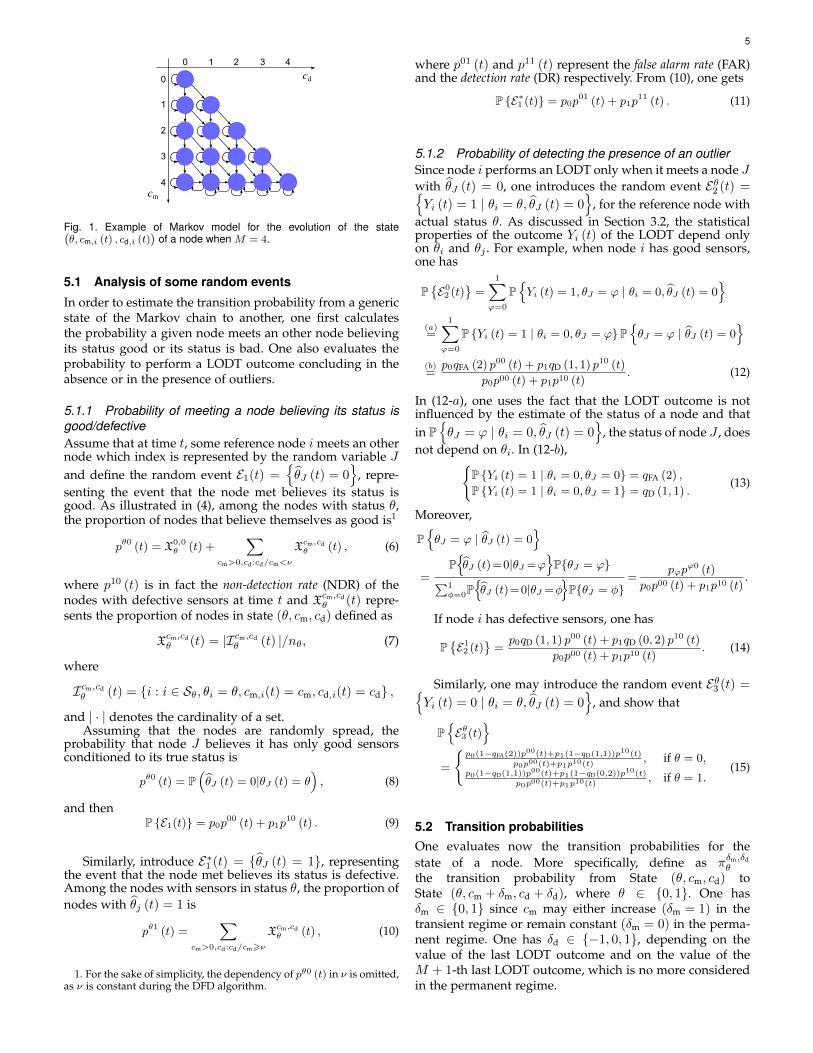
node is (M + 1) (M + 2) /2. The evolution of xi (t), condi-tioned by its status θi, follows a Markov model with statetransition diagram of the kind shown in Figure 1 for M = 4.
In particular, there are two chains, one conditionedby θi = 0 and the other conditioned by θi = 1. Bothare characterized by a transient phase for state valueswith cm,i(t) < M ; then, a permanent regime starts whencm,i(t) = M . With cm,i (t) = cm and cd,i (t) = cd, the tran-sitions from State (θ, cm, cd) to State (θ, c′m, c
′d) are analyzed
in the following.
5
0
0
1
2
3
4
1 2 3 4
cd
cm
Fig. 1. Example of Markov model for the evolution of the state(θ, cm,i (t) , cd,i (t)
)of a node when M = 4.
5.1 Analysis of some random events
In order to estimate the transition probability from a genericstate of the Markov chain to another, one first calculatesthe probability a given node meets an other node believingits status good or its status is bad. One also evaluates theprobability to perform a LODT outcome concluding in theabsence or in the presence of outliers.
5.1.1 Probability of meeting a node believing its status isgood/defectiveAssume that at time t, some reference node i meets an othernode which index is represented by the random variable Jand define the random event E1(t) =
{θJ (t) = 0
}, repre-
senting the event that the node met believes its status isgood. As illustrated in (4), among the nodes with status θ,the proportion of nodes that believe themselves as good is1
pθ0 (t) = X0,0θ (t) +
∑cm>0,cd:cd/cm<ν
Xcm,cdθ (t) , (6)
where p10 (t) is in fact the non-detection rate (NDR) of thenodes with defective sensors at time t and X
cm,cdθ (t) repre-
sents the proportion of nodes in state (θ, cm, cd) defined as
Xcm,cdθ (t) = |Icm,cd
θ (t) |/nθ, (7)
where
Icm,cdθ (t) = {i : i ∈ Sθ, θi = θ, cm,i(t) = cm, cd,i(t) = cd} ,
and | · | denotes the cardinality of a set.Assuming that the nodes are randomly spread, the
probability that node J believes it has only good sensorsconditioned to its true status is
pθ0 (t) = P(θJ (t) = 0|θJ (t) = θ
), (8)
and thenP {E1(t)} = p0p
00 (t) + p1p10 (t) . (9)
Similarly, introduce E∗1 (t) = {θJ (t) = 1}, representingthe event that the node met believes its status is defective.Among the nodes with sensors in status θ, the proportion ofnodes with θj (t) = 1 is
pθ1 (t) =∑
cm>0,cd:cd/cm>ν
Xcm,cdθ (t) , (10)
1. For the sake of simplicity, the dependency of pθ0 (t) in ν is omitted,as ν is constant during the DFD algorithm.
where p01 (t) and p11 (t) represent the false alarm rate (FAR)and the detection rate (DR) respectively. From (10), one gets
P {E∗1 (t)} = p0p01 (t) + p1p
11 (t) . (11)
5.1.2 Probability of detecting the presence of an outlierSince node i performs an LODT only when it meets a node Jwith θJ (t) = 0, one introduces the random event Eθ2 (t) ={Yi (t) = 1 | θi = θ, θJ (t) = 0
}, for the reference node with
actual status θ. As discussed in Section 3.2, the statisticalproperties of the outcome Yi (t) of the LODT depend onlyon θi and θj . For example, when node i has good sensors,one has
P{E02 (t)
}=
1∑ϕ=0
P{Yi (t) = 1, θJ = ϕ | θi = 0, θJ (t) = 0
}(a)=
1∑ϕ=0
P {Yi (t) = 1 | θi = 0, θJ = ϕ}P{θJ = ϕ | θJ (t) = 0
}(b)=p0qFA (2) p00 (t) + p1qD (1, 1) p10 (t)
p0p00 (t) + p1p10 (t). (12)
In (12-a), one uses the fact that the LODT outcome is notinfluenced by the estimate of the status of a node and thatin P
{θJ = ϕ | θi = 0, θJ (t) = 0
}, the status of node J , does
not depend on θi. In (12-b),{P {Yi (t) = 1 | θi = 0, θJ = 0} = qFA (2) ,
P {Yi (t) = 1 | θi = 0, θJ = 1} = qD (1, 1) .(13)
Moreover,
P{θJ = ϕ | θJ (t) = 0
}=
P{θJ (t)=0|θJ =ϕ
}P{θJ = ϕ}∑1
φ=0P{θJ (t)=0|θJ =φ
}P{θJ = φ}
=pϕp
ϕ0 (t)
p0p00 (t) + p1p10 (t).
If node i has defective sensors, one has
P{E12 (t)
}=p0qD (1, 1) p00 (t) + p1qD (0, 2) p10 (t)
p0p00 (t) + p1p10 (t). (14)
Similarly, one may introduce the random event Eθ3 (t) ={Yi (t) = 0 | θi = θ, θJ (t) = 0
}, and show that
P{Eθ3 (t)
}=
{p0(1−qFA(2))p
00(t)+p1(1−qD(1,1))p10(t)
p0p00(t)+p1p10(t), if θ = 0,
p0(1−qD(1,1))p00(t)+p1(1−qD(0,2))p
10(t)
p0p00(t)+p1p10(t), if θ = 1.
(15)
5.2 Transition probabilitiesOne evaluates now the transition probabilities for thestate of a node. More specifically, define as πδm,δd
θthe transition probability from State (θ, cm, cd) toState (θ, cm + δm, cd + δd), where θ ∈ {0, 1}. One hasδm ∈ {0, 1} since cm may either increase (δm = 1) in thetransient regime or remain constant (δm = 0) in the perma-nent regime. One has δd ∈ {−1, 0, 1}, depending on thevalue of the last LODT outcome and on the value of theM + 1-th last LODT outcome, which is no more consideredin the permanent regime.
6
Thus, (δm, δd) ∈ {(0, 0) , (0, 1) , (0,−1) (1, 0) , (1, 1) , (1,−1)}.Note that πδm,δd
θ depends on the current state of the referencenode, but also on the current proportion of active (goodand defective) nodes. Therefore, the transition probabilitiesare denoted as πδm,δd
θ (t, cm, cd), where t is the time instant,cm,i(t) = cm, and cd,i(t) = cd. Depending on the value ofcm, two different cases are considered in Section 5.2.1 andin Section 5.2.2, respectively corresponding to the transientand permanent regimes.
5.2.1 Case I, cm,i(t) < M
In the transient regime, when cm,i(t) < M , cm,i(t) andcd,i(t) are updated according to (3) whenever node J withθJ (t) = 0 is met. The only possibility that leads to δm = 0is the event E∗1 , i.e., node i meets node J with θJ (t) = 1. Asa consequence, no LODT is performed by node i. Therefore,for any θ ∈ {0, 1},
π0,0θ (t, cm, cd) = P {E∗1 (t)} = p0p
01 (t) + p1p11 (t) , (16)
where pθ1 (t) is defined by (10).A state transition occurs with (δm, δd) = (1, 1) when
node i with status θi = θ meets node J with θJ (t) = 0and when the LODT yields yi (t) = 1. Since the two eventsare independent, one has
π1,1θ (t, cm, cd) = P
{Yi (t) = 1, θJ (t) = 0|θi = θ
}= P {E1 (t)}P
{Eθ2 (t)
}. (17)
Depending on the value of θi, using (9), (12), and (14), onemay rewrite (17) as
π1,1θ (t, cm, cd)=
{p0qFA (2) p00 (t) + p1qD (1, 1) p10 (t) , if θ = 0,
p0qD (1, 1) p00 (t) + p1qD (0, 2) p10 (t) , if θ = 1.
(18)
Finally, π1,0θ (t, cm, cd) = P
{Yi (t) = 0, θJ (t) = 0|θi = θ
}is
obtained similarly from (15)
π1,0θ (t, cm, cd) ={p0 (1− qFA (2)) p00 (t) + p1 (1− qD (1, 1)) p10 (t) , if θ = 0,
p0 (1− qD (1, 1)) p00 (t) + p1 (1− qD (0, 2)) p10 (t) , if θ = 1.
(19)
5.2.2 Case II, cm,i(t) = M
In the permanent regime, cm,i(t) = M and does not increaseany more, thus δm = 0. In Algorithm 2, µ is the number ofLODTs performed by node i up to time t. When µ >M , onlythe last M LODT outcomes are considered: LODT outcomesymi with m 6 µ−M are no more considered.
To determine the value taken by δd ∈ {−1, 0, 1} after theµ-th LODT, consider the random event
E14 (t) =
{Y µ−Mi = 1 |
µ−1∑m=µ−M
Y mi = cd
}, (20)
which corresponds to a situation where one knows thatcd LODTs where positive among the last M tests and theLODT that will be ignored, once the new LODT outcomeis available, also concluded in the presence of defectivesensors. P
{E14 (t)
}is relatively complex to evaluate, since
P {Y ni = 1} is time-varying according to (12-14). In whatfollows, we assume that LODT outcomes with Y mi = 1
are independently distributed over the time horizon corre-sponding to m = µ−M, . . . , µ− 1. One obtains then
P{E14 (t)
}=cd
M. (21)
This approximation is exact in steady-state, when the Xcm,cdθ s
do not vary any more.Similarly, define
E04 (t) =
{Y µ−Mi = 0 |
µ−1∑m=µ−M
Y mi = cd
}. (22)
Considering the same assumption used to get (21), one has
P{E04 (t)
}= 1− P
{E14 (t)
}≈ M − cd
M. (23)
Assume that the (µ−M)-th LODT performed by node ioccurred at time t, then yµ−Mi can also be denoted as yi
(t)
and the transition related to cd,i is such that δd = yi (t) −yi(t)∈ {−1, 0, 1} .
To have (δm, δd) = (0, 1), three independent events haveto occur: 1) the encountered node J believes it is good attime t, i.e., E1 (t); 2) yi (t) = 1, i.e., Eθ3 (t) (t); 3) yi
(t)
= 0,i.e., E04 (t). Thus the transition probability may be expressedas
π0,1θ (t,M, cd) = P{E1 (t)}P{Eθ3 (t)}P{E04 (t)}. (24)
Using (9), (12), (14), and (21) in (24), one gets
π0,1θ (t,M, cd)
=
{(p0qFA(2) p00 (t) + p1qD(1, 1) p10 (t)
)M−cdM
, if θ = 0,(p0qD(1, 1) p00 (t) + p1qD(0, 2) p10 (t)
)M−cdM
, if θ = 1.(25)
Consider now (δm, δd) = (0,−1). To have such transi-tion, the three following independent events should occur:1) E1 (t); 2) yi (t) = 0, i.e., Eθ3 (t) (t); 3) yi
(t)
= 1, i.e., E14 (t).Thus, the transition probability is
π0,−1θ (t,M, cd) = P{E1 (t)}P{Eθ3 (t)}P{E14 (t)}
=
{(p0(1−qFA (2)) p00 (t) + p1(1−qD (1, 1)) p10 (t)
)cdM, if θ = 0,(
p0(1−qD (1, 1)) p00 (t) + p1(1−qD (0, 2)) p10 (t))cdM, if θ = 1.
(26)
Finally, by substituting eqs. (25-26) it is possible to calcu-late π0,0
θ (t,M, cd) which is given by
π0,0θ (t,M, cd) = 1− π0,1
θ (t,M, cd)− π0,−1θ (t,M, cd) . (27)
In this section, we have so far completely characterizedthe transition probabilities between any possible pair ofstates in the Markov chain. Accordingly, we are now ableto completely describe the evolution of the DTN state com-ponents and, thus, the expected proportion of nodes in aspecific state.
6 MACROSCOPIC EVOLUTION OF THE DTN STATEAll node state transition probabilities evaluated in Section 5are now used to determine the evolution of the proportionof nodes in state θ, i.e.
Xθ (t)=(X0,0θ (t) ,X1,0
θ (t) ,X1,1θ (t) , . . . ,XM,0θ (t) , . . . ,XM,Mθ (t)
)and the corresponding expected values
Xθ (t)=(X0,0θ (t) , X1,0
θ (t) , X1,1θ (t) , . . . , XM,0
θ (t) , . . . , XM,Mθ (t)
).
7
Proposition 2. The evolution of the DTN state components, i.e.,the expected proportion of nodesXcm,cd
θ (t) in the states (θ, cm, cd),with θ ∈ {0, 1}, cm = 0, . . . ,M , and cd 6 cm is described by
dX0,0θdt
(a)= −λX0,0
θ
(π1,0θ (0, 0) + π1,1
θ (0, 0)),
dXcm,0θdt
(b)= λ
(−Xcm,0
θ
(π1,0θ (cm, 0) + π1,1
θ (cm, 0))
+Xcm−1,0θ π1,0
θ (cm − 1, 0)),
dXcm,cmθdt
(c)= λ
(−Xcm,cm
θ
(π1,0θ (cm, cm) + π1,1
θ (cm, cm))
+Xcm−1,cm−1θ π1,1
θ (cm − 1, cm − 1)),
dXM,0θdt
(d)= λ
(−XM,0
θ π0,1θ (M, 0) +XM−1,0
θ π1,0θ (M − 1, 0)
+XM,1θ π0,−1
θ (M, 1)),
dXM,Mθdt
(e)= λ
(−XM,M
θ π0,−1θ (M,M)+XM,M−1
θ π0,1θ (M,M−1)
+ XM−1,M−1θ π1,1
θ (M − 1,M − 1)),
(28)for any cm = 1, . . . ,M−1, with the initial conditionsX0,0
θ (0) =1 and Xcm,cd
θ (0) = 0, ∀cm, cd 6= 0.
Proof: See Appendix AKurtz’s theorem [33], [34] can then be used to show that
for all ε > 0, there exists α1 > 0 and α2 (ε) > 0 such that
Pr
(maxt∈[0,T ]
‖Xθ (t)−Xθ (t)‖ > ε
)6 α1 exp (−α2 (ε)nθ) .
As a consequence, Xθ (t) converges in probability to Xθ (t)as nθ goes to infinity. This is typically the approximationperformed in the seminal work [35] where the SIR modelwas proposed. This model is the one used to characterizemost widely studied classes of epidemic models. Accord-ingly, analogously to what was presented for example in[7], [35]–[40], the proposed system consists of ordinary dif-ferential equations approximating jump Markov processes.
The state equations in (28) are nonlinear, since each πδm,δdθ
depends on Xcm,cdθ , see (6) and (10).
7 ANALYSIS OF THE DTN STATE EQUATIONS
In what follows, the asymptotic behavior of the DTN stateequations (28) is characterized. Algorithm 2 may driveXcm,cdθ to an equilibrium X
cm,cd
θ at which the proportionsof nodes in different states Xcm,cd
θ (t) do not vary any more.As a consequence, pθ0 (t) defined in (6) also tends to anequilibrium pθ0.
7.1 Equilibrium of Xcm,cdθ
One investigates first the evolution of Xcm,cdθ (t) when cm <
M . As shown in the following proposition, the DTN statealways reaches the permanent regime.
Proposition 3. For any cm < M and cd 6 cm, limt→∞
Xcm,cdθ (t) =
0.
Proof: See Appendix B.From Proposition 3, the only possible value at equilib-
rium of Xcm,cdθ (t) when cm < M is 0. Thus pθ0 may be
written aspθ0 =
∑cd:cd/M<ν
XM,cdθ . (29)
Denote p =(p00, p10
)∈ P0 with
P0 = {(x, y) ∈ [0, 1]× [0, 1] and (x, y) 6= (0, 0)} (30)
and consider the functions
h0 (p) =p0qFA (2) p00 + p1qD (1, 1) p10
p0p00 + p1p10, (31)
h1 (p) =p0qD (1, 1) p00 + p1qD (0, 2) p10
p0p00 + p1p10, (32)
Fθ (p) =
dMνe−1∑cd=0
(M
cd
)(hθ (p))cd (1− hθ (p))M−cd , (33)
and F (p) = (F0 (p) , F1 (p)). The following propositionprovides a non-linear equation that has to be satisfied by p.The various X
M,cd
θ at equilibrium are easily deduced fromthe solutions of the mentioned equation.
Proposition 4. Assume that the dynamic system described by(28) admits some equilibrium X
cm,cd
θ , then p ∈ P0 is the solutionof
p = F (p) , (34)
and for any θ ∈ {0, 1} and cd 6 cm,
Xcm,cdθ =
{0, ∀cm < M,(Mcd
)(hθ (p))cd (1− hθ (p))M−cd , cm = M.
(35)
Proof: See Appendix C.
7.2 Existence and uniqueness of the equilibrium pointNow we investigate the existence and the uniqueness of thesolution of (34), which is rewritten in detail in (36) at the topof the next page.
For that purpose, using fixed-point theorems, one mayalternatively show that for all p (0) =
(p00 (0) , p10 (0)
)∈
P0, the discrete-time system{p00 (n+ 1) = F0
(p00 (n) , p10 (n)
),
p10 (n+ 1) = F1
(p00 (n) , p10 (n)
).
(39)
converges to a unique equilibrium point(p00, p10
), which is
then solution of (36).One first shows the existence of an equilibrium using
Brouwer’s fixed-point theorem [41] in the following propo-sition.
Proposition 5. For any ν ∈ [0, 1], (36) always admits a solution,which is an equilibrium point of the dynamical system (28).
Before proving Proposition 5, one first shows that p00 (n)and p10 (n) are contained in intervals with lower (andupper) bounds increasing (resp. decreasing) with n.
Lemma 6. For any n ∈ N∗ and θ ∈ {0, 1}, one has
pθ0min (n) 6 pθ0 (n) 6 pθ0max (n) ,
with pθ0min (0) = 0, pθ0max (0) = 1, and{pθ0min (n+ 1) = Fθ
(p00min (n) , p10max (n)
), ∀n ∈ N+,
pθ0max (n+ 1) = Fθ(p00max (n) , p10min (n)
), ∀n ∈ N+.
(40)
Moreover,
p00min (n+ 1) > p00min (n) , p00max (n+ 1) < p00max (n) . (41)
Proof: See Appendix D.Using Lemma 6, one can now prove Proposition 5.
Proof: F0 and F1 are both continuous functions. Forsome n > 0, consider the set Pn =
[p00min (n) , p00max (n)
]×[
p10min (n) , p10max (n)], where pθ0min (n) and pθ0max (n) are defined
8 p00 = F0
(p00, p10
)=∑cd:cd/M<ν
(Mcd
) (p0qFA(2)p00+p1qD(1,1)p
10
p0p00+p1p10
)cd(p0(1−qFA(2))p
00+p1(1−qD(1,1))p10
p0p00+p1p10
)M−cd
,
p10 = F1
(p00, p10
)=∑cd:cd/M<ν
(Mcd
) (p0qD(1,1)p00+p1qD(0,2)p
10
p0p00+p1p10
)cd(p0(1−qD(1,1))p
00+p1(1−qD(0,2))p10
p0p00+p1p10
)M−cd
.(36)
c0(qFA(2), qD(0,2),qD(1,1), p1,M, ν, n)=M (qD (1,1)− qFA (2)) p0p1p
00max (n) p10max (n)
(p0p00min(n)+p1p10min(n))((1− qFA(2))p0p00min(n)+(1− qD(1,1))p1p10min(n)), (37)
c1(qFA(2), qD(0,2),qD(1,1), p1,M, ν, n)=M (qD (0,2)− qD (1,1)) p0p1p
00max (n) p10max (n)
(p0p00min(n)+p1p10min(n))((1− qD(1,1))p0p00min(n)+(1− qD(0,2))p1p10min(n)), (38)
0 0.05 0.1 0.15 0.2 0.25 0.3 0.35 0.4 0.45 0.5
0.4
0.5
0.6
0.7
0.8
0.9
1
p1
νm
ax
M=4, qD
(1,1)=0.8
M=4, qD
(1,1)=0.5
M=10, qD
(1,1)=0.8
M=10, qD
(1,1)=0.5
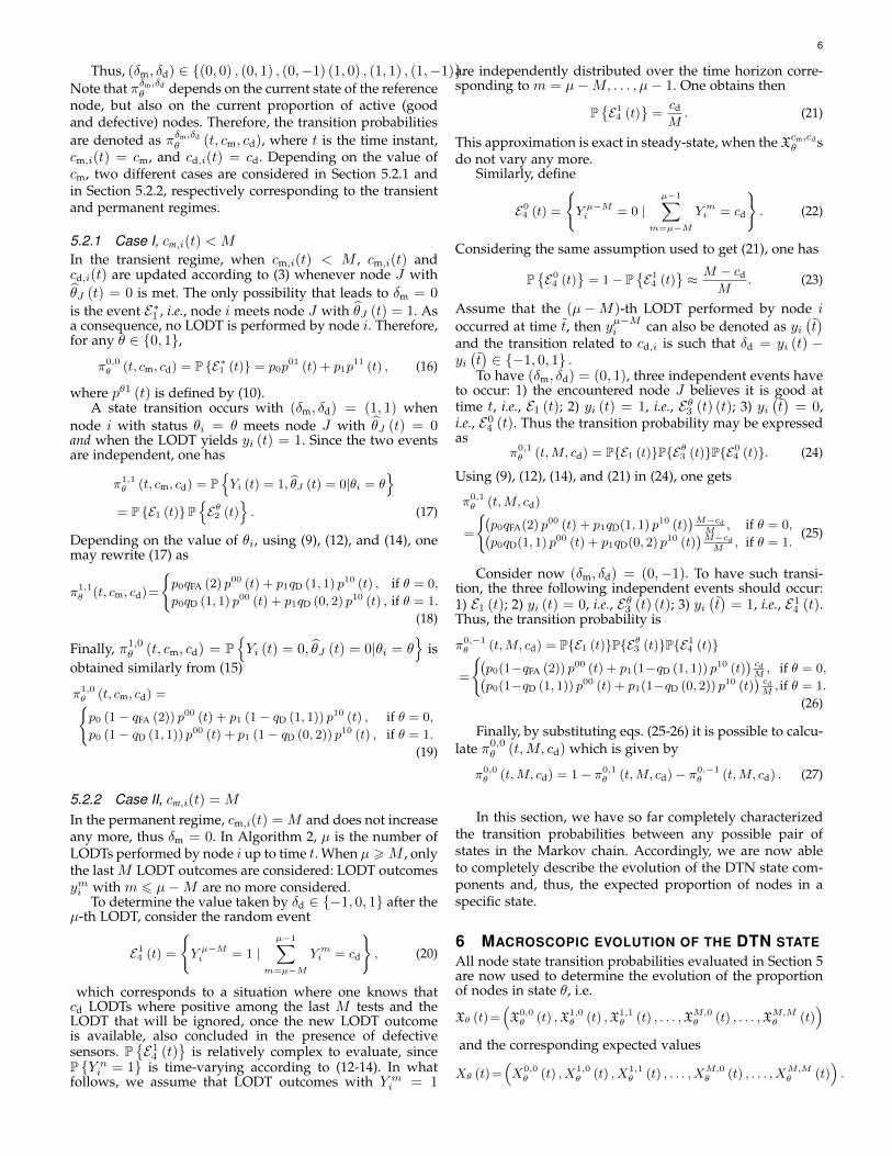
Fig. 2. Upper bounds of ν to satisfy (42), with qFA (2) = 0.05, qD (0, 2) =0.9, qD (1, 1) ∈ {0.5, 0.8}, M ∈ {4, 10}, and p1 ∈ [0.05, 0.5].
in (40). For any p =(p00, p10
)∈ Pn, one can prove using
Lemma 6 that F (p) ∈ Pn. Thus F maps Pn to Pn. ApplyingBrouwer’s fixed-point theorem, F admits a fixed point andProposition 5 is proved.
Sufficient conditions on p0, p1, qD, qFA, M and ν are thenprovided to ensure the uniqueness of this equilibrium byapplying Banach’s fixed-point theorem [42].
Proposition 7. If there exists some N ′, such that ∀θ ∈ {0, 1}and ∀n > N ′, one has
cθ(qFA(2), qD(0, 2),qD (1, 1), p1,M, ν, n)< 1, (42)
where c0 and c1 are defined in (37-38), then the discrete-timesystem (39) converges to a unique equilibrium point and thesolution of (36) is unique.
Proof: See Appendix E.Due to the monotonicity of pθ0min (n) and pθ0max (n) shown
in Lemma 6, cθ decreases with n. Hence, if a given ν satisfies(42) for some N ′, then ν will satisfy (42) for all n > N ′
and the equilibrium is unique. If the values of p1, qD, qFA,and M are fixed, then one may deduce sufficient conditionson the value of ν to have a unique equilibrium point. SeeExample 8.
Example 8. Consider qFA (2) = 0.05, qD (0, 2) = 0.9,qD (1, 1) ∈ {0.5, 0.8}, M ∈ {4, 10}, and p1 ∈ [0.05, 0.5].One verifies whether (42) is satisfied considering n = 10for different values of ν. One obtains that (42) holds if0 < ν 6 νmax, where νmax depends on the values of p1,qD, qFA, and M . See Figure 2 for the numerical values ofνmax in each case.
7.3 Equilibrium point as M →∞Both p00 and p10 can be seen as functions ofM . AsM →∞,Algorithm 2 turns into Algorithm 1. In this situation, if ν is
properly chosen, the probabilities of false alarm and non-detection tend to zero, as shown in Proposition 9.
Proposition 9. If qFA (2) < ν < qD (1, 1), then (36) has aunique solution and
limM→∞
p00 = 1, limM→∞
p10 = 0. (43)
Proof: See Appendix F.
7.4 Approximations of the EquilibriumClosed-form expressions for p00 and p10 are difficult toobtain from (36). This section introduces an approximationof (36) from which some insights may be obtained on theway ν should be chosen.
Since p10 represents the expected proportion of nodeswith defective sensors that have not detected their status,the value of p10 should be small. From (31-32) one sees thatlimp10→0 h0 = qFA (2) and limp10→0 h1 = qD (1, 1), thus onemay consider the following approximations
h0 ≈ h0 = qFA (2) , h1 ≈ h1 = qD (1, 1) . (44)
Therefore, (36) may be rewritten as{p00 =
∑cd:cd/M<ν
(Mcd
)(qFA (2))cd (1− qFA (2))M−cd ,
p10 =∑cd:cd/M<ν
(Mcd
)(qD (1, 1))cd (1− qD (1, 1))M−cd .
(45)from which one deduces approximate values XM,cd
0 ofXM,cd
0 at equilibrium from eq. (35){XM,cd
0 =(Mcd
)(qFA (2))cd (1− qFA (2))M−cd ,
XM,cd1 =
(Mcd
)(qD (1, 1))cd (1− qD (1, 1))M−cd .
(46)
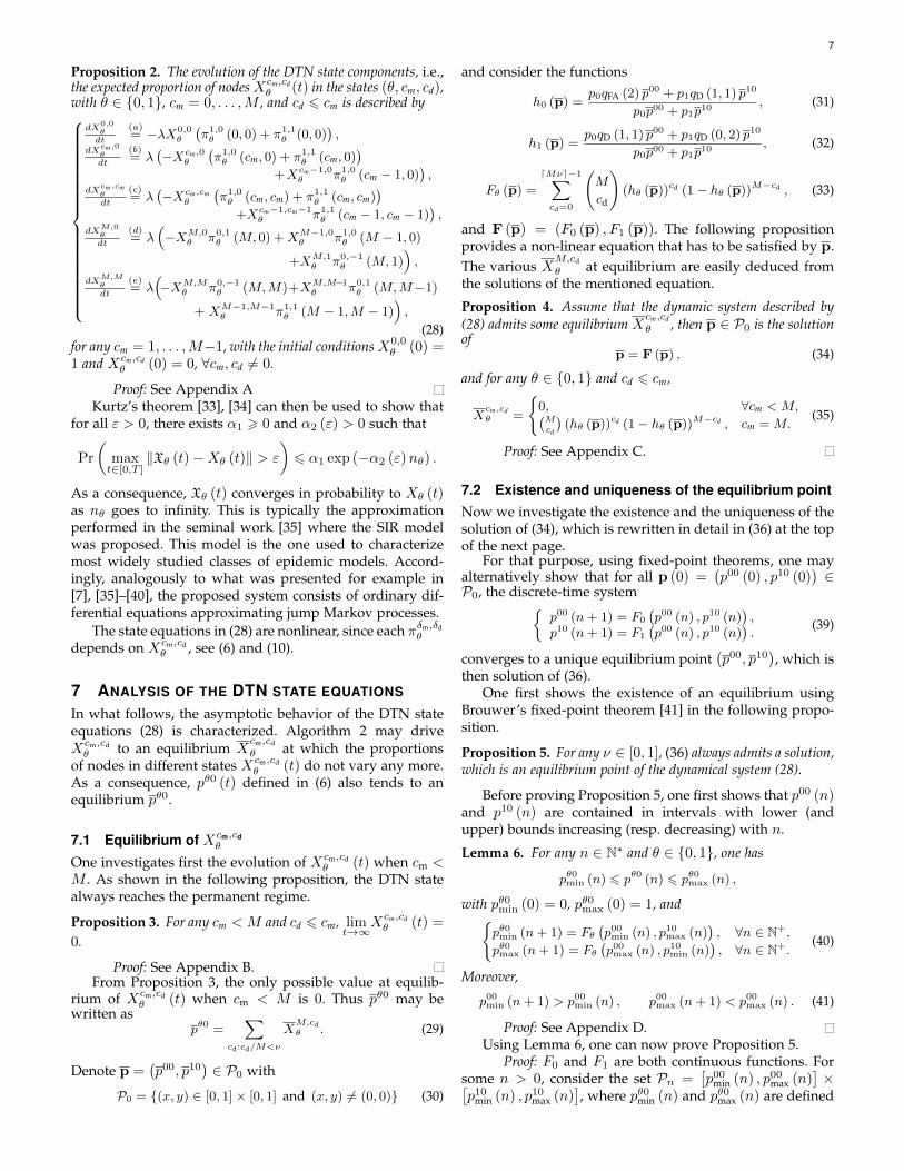
For any fixed value of M , qFA (2), and qD (1, 1), thevalues of detection rate (p11) and false alarm rate (p01) at equi-librium can be predicted using (45), since p01 = 1− p00 andp11 = 1−p10. Consider for example M = 10, qFA (2) = 0.05,and qD (1, 1) = 0.8. Figure 3 presents p11 as a function of p01
for different values of ν. This figure is helpful to choose thevalue of ν to meet different performance requirements. Theactual values of p11 and p01 are also shown in Figure 3,which are very close to p11 and p01, in the region where p11
is close to 1.
8 INFLUENCE OF MISBEHAVING NODES
A LODT involving data coming from a misbehaving nodewill always result in the detection of an outlier. Thus, whena node i with state xi(t) = (θ, cm,i (t) , cd,i (t)) meets amisbehaving node, the possible transitions are such that
• (δm, δd) = (1, 0) or (δm, δd) = (1, 1) if cm,i (t) < M
9
10−15
10−10
10−5
100
0
0.2
0.4
0.6
0.8
1
p01=1−p00
p11=
1−p10
qD
(1.1)=0.8, actual value
qD
(1.1)=0.8, approximation
qD
(1.1)=0.5, actual value
qD
(1.1)=0.5, approximation
ν=0.2ν=0.4
ν=1
Fig. 3. Approximate p11 as a function of approximate p01, for various νand fixed M = 10 .
• (δm, δd) = (0, 0) or (δm, δd) = (0, 1) if cm,i (t) = Mand 0 < cd,i (t) < M
• (δm, δd) = (0, 0) if cm,i (t) = cd,i (t) = M .
Then, in the evaluation of the probability of the eventsE∗1 (t), Eθ2 (t), and Eθ3 (t) introduced in Section 5, one has toaccount for the probability of meeting a misbehaving node.For example, (11) can be rewritten as
P {E∗1 (t)} = p0p01 (t) + p1p
11 (t) + p2. (47)
The transition probabilities introduced in Sections 5.2.1and 5.2.2 have to be updated accordingly. The form of theDTN state equations (28) remains the same.
Finally, the effect misbehaving nodes can be taken intoaccount in (45) for the computation of the approximateexpressions of p00 and p10. More specifically, p00 =
∑cd:cd/M<ν
(Mcd
) ( p0qFA(2)+p2p0+p2
)cd(
1− p0qFA(2)+p2p0+p2
)M−cd,
p10 =∑cd:cd/M<ν
(Mcd
) ( p0qD(1,1)+p2p0+p2
)cd(
1− p0qD(1,1)+p2p0+p2
)M−cd.
(49)
9 NUMERICAL RESULTS
In this Section we provide results aimed at assessing theconvergence of the theoretical framework (Section 10.1),the appropriateness and accuracy of the framework alsoin case of specific mobility models such as the Brownianmotion (Section 10.2) or other more realistic mobility modelsderived from user traces (Section 10.3), as well as to comparethe proposed DFD methodology to other state-of-the-art so-lutions (Section 10.4). Finally, in Section 10.5 we investigateon the stability and accuracy of the Algorithm upon varyingsome key parameters.
9.1 Numerical verification of theoretical resultsThis section presents first the solution of the state equation(28) describing the evolution of the proportion of nodesin various states. Algorithm 2 is simulated considering arandom displacement of nodes without any constraint ontheir speed. This allows to verify the correctness of thetheoretical results presented in this paper.
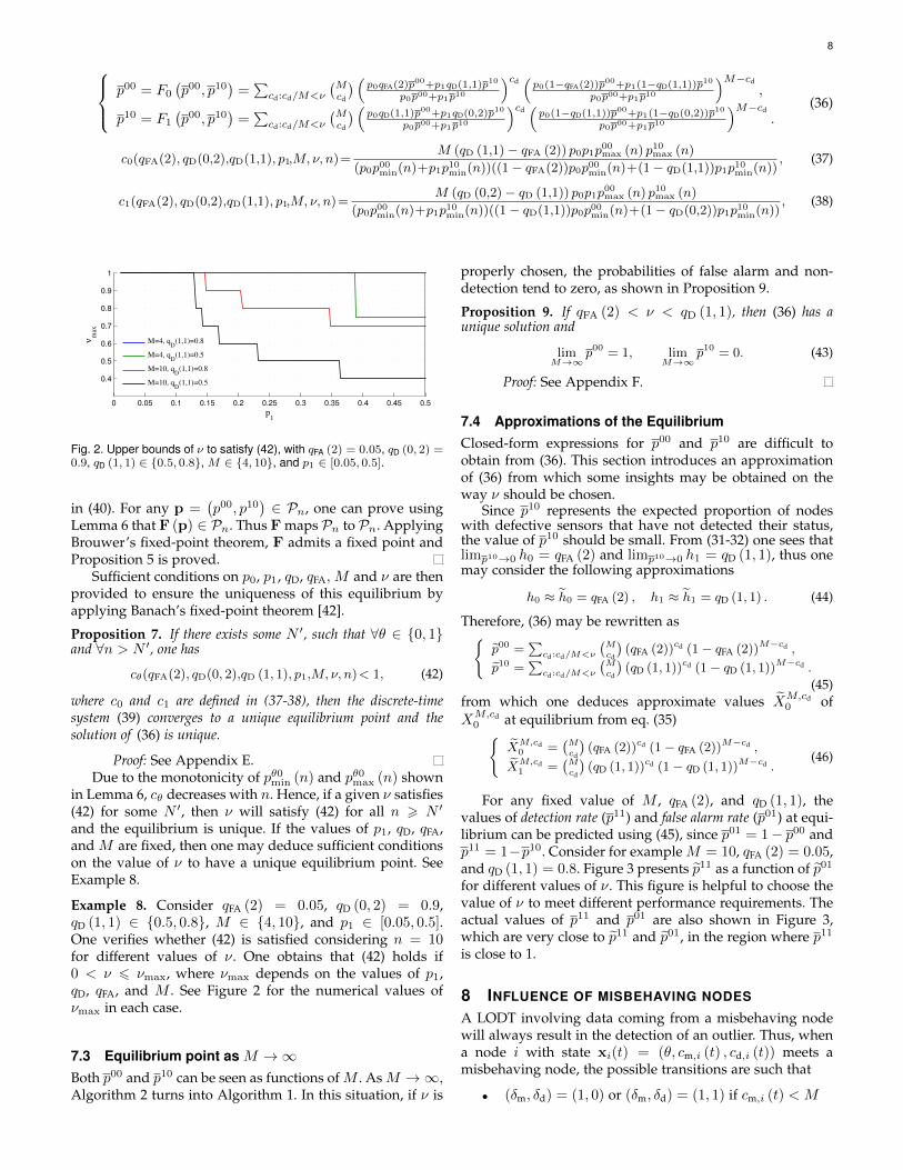
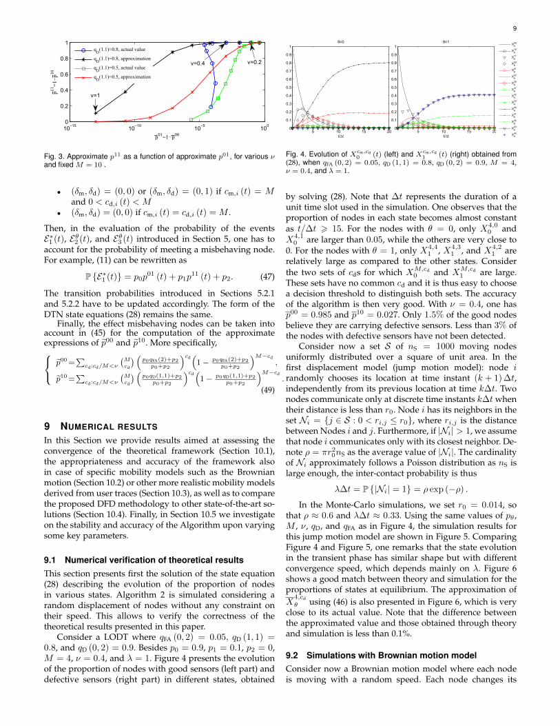
Consider a LODT where qFA (0, 2) = 0.05, qD (1, 1) =0.8, and qD (0, 2) = 0.9. Besides p0 = 0.9, p1 = 0.1, p2 = 0,M = 4, ν = 0.4, and λ = 1. Figure 4 presents the evolutionof the proportion of nodes with good sensors (left part) anddefective sensors (right part) in different states, obtained
5 10 15 200
0.1
0.2
0.3
0.4
0.5
0.6
0.7
0.8
0.9
1
t/∆t
θ=0
5 10 15 200
0.1
0.2
0.3
0.4
0.5
0.6
0.7
0.8
0.9
1
t/∆t
θ=1X00θ
X10θ
X11θ
X20θ
X21θ
X22θ
X30θ
X31θ
X32θ
X33θ
X40θ
X41θ
X42θ
X43θ
X44θ
Fig. 4. Evolution of Xcm,cd0 (t) (left) and Xcm,cd
1 (t) (right) obtained from(28), when qFA (0, 2) = 0.05, qD (1, 1) = 0.8, qD (0, 2) = 0.9, M = 4,ν = 0.4, and λ = 1.
by solving (28). Note that ∆t represents the duration of aunit time slot used in the simulation. One observes that theproportion of nodes in each state becomes almost constantas t/∆t > 15. For the nodes with θ = 0, only X4,0
0 andX4,1
0 are larger than 0.05, while the others are very close to0. For the nodes with θ = 1, only X4,4
1 , X4,31 , and X4,2
1 arerelatively large as compared to the other states. Considerthe two sets of cds for which XM,cd
0 and XM,cd1 are large.
These sets have no common cd and it is thus easy to choosea decision threshold to distinguish both sets. The accuracyof the algorithm is then very good. With ν = 0.4, one hasp00 = 0.985 and p10 = 0.027. Only 1.5% of the good nodesbelieve they are carrying defective sensors. Less than 3% ofthe nodes with defective sensors have not been detected.
Consider now a set S of nS = 1000 moving nodesuniformly distributed over a square of unit area. In thefirst displacement model (jump motion model): node irandomly chooses its location at time instant (k + 1) ∆t,independently from its previous location at time k∆t. Twonodes communicate only at discrete time instants k∆t whentheir distance is less than r0. Node i has its neighbors in theset Ni = {j ∈ S : 0 < ri,j ≤ r0}, where ri,j is the distancebetween Nodes i and j. Furthermore, if |Ni| > 1, we assumethat node i communicates only with its closest neighbor. De-note ρ = πr20nS as the average value of |Ni|. The cardinalityof Ni approximately follows a Poisson distribution as nS islarge enough, the inter-contact probability is thus
λ∆t = P {|Ni| = 1} = ρ exp (−ρ) .
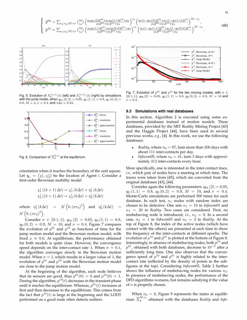
In the Monte-Carlo simulations, we set r0 = 0.014, sothat ρ ≈ 0.6 and λ∆t ≈ 0.33. Using the same values of pθ ,M , ν, qD, and qFA as in Figure 4, the simulation results forthis jump motion model are shown in Figure 5. ComparingFigure 4 and Figure 5, one remarks that the state evolutionin the transient phase has similar shape but with differentconvergence speed, which depends mainly on λ. Figure 6shows a good match between theory and simulation for theproportions of states at equilibrium. The approximation ofX
4,cd
θ using (46) is also presented in Figure 6, which is veryclose to its actual value. Note that the difference betweenthe approximated value and those obtained through theoryand simulation is less than 0.1%.
9.2 Simulations with Brownian motion modelConsider now a Brownian motion model where each nodeis moving with a random speed. Each node changes its
10 p00 =∑cd:cd/M<ν
(Mcd
) (p0qFA(2)p00+p1qD(1,1)p
10+p2p0p00+p1p10+p2
)cd(p0(1−qFA(2))p
00+p1(1−qD(1,1))p10
p0p00+p1p10+p2
)M−cd
,
p10 =∑cd:cd/M<ν
(Mcd
) (p0qD(1,1)p00+p1qD(0,2)p
10+p2p0p00+p1p10+p2
)cd(p0(1−qD(1,1))p
00+p1(1−qD(0,2))p10
p0p00+p1p10+p2
)M−cd
.(48)
0 5 10 15 20 25 30 350
0.1
0.2
0.3
0.4
0.5
0.6
0.7
0.8
0.9
1
t/∆t
θ=0
0 5 10 15 20 25 30 350
0.1
0.2
0.3
0.4
0.5
0.6
0.7
0.8
0.9
1
t/∆t
θ=1Xθ00
Xθ10
Xθ11
Xθ20
Xθ21
Xθ22
Xθ30
Xθ31
Xθ32
Xθ33
Xθ40
Xθ41
Xθ42
Xθ43
Xθ44
Fig. 5. Evolution of Xcm,cd0 (t) (left) and Xcm,cd
1 (t) (right) by simulationswith the jump model, when qFA (0, 2) = 0.05, qD (1, 1) = 0.8, qD (0, 2) =0.9, M = 4, ν = 0.4, and λ∆t = 0.33.
0 1 2 3 40
0.2
0.4
0.6
0.8
1
cd
X04,cd, theory
X04,cd, simulation
X04,cd, approximation
X14,cd
X14,cd
X14,cd, approximation
, theory
, simulation
Fig. 6. Comparison of X4,cdθ at the equilibrium.
orientation when it reaches the boundary of the unit square.Let χi =
(χi1, χ
i2
)be the location of Agent i. Consider a
first-order Brownian mobility model
χi1 ((k + 1) ∆t) = χi1 (k∆t) + ηi1 (k∆t)
χi2 ((k + 1) ∆t) = χi2 (k∆t) + ηi2 (k∆t)
where ηi1 (k∆t) ∼ N(
0, (σr0)2)
and ηi2 (k∆t) ∼
N(
0, (σr0)2)
.
Consider σ ∈ {0.1, 1}, qFA (2) = 0.05, qD (1, 1) = 0.8,qD (0, 2) = 0.9, M = 10, and ν = 0.4. Figure 7 comparesthe evolution of p01 and p10 as functions of time for thejump motion model and the Brownian motion model, withfixed ρ ≈ 0.6. At equilibrium, the performance obtainedfor both models is quite close. However, the convergencespeed depends on the inter-contact rate λ. When σ = 0.1,the algorithm converges slowly in the Brownian motionmodel. When σ = 1, which results in a larger value of λ, theevolution of p01 and p10 with the Brownian motion modelare close to the jump motion model.
At the beginning of the algorithm, each node believesthat its sensors are good, thus p01(0) = 0 and p10(0) = 1.During the algorithm, p10(t) decreases in the transient phaseuntil it reaches the equilibrium. Whereas, p01(t) increases atfirst and then decreases to the equilibrium. This comes fromthe fact that p10(t) is large at the beginning and the LODTperformed on a good node often detects outliers.
0 20 40 60 80 10010
−3
10−2
10−1
100
σ=1
p01, Brownian,
p01, Brownian,
σ=0.1
p10, Brownian, σ=1
p01, Jump Model
p10, Brownian,
p10, Jump Model
σ=0.1
Fig. 7. Evolution of p01 and p10 for the two moving models, with σ ∈{0.1, 1}, qFA (2) = 0.05, qD (1, 1) = 0.8, qD (0, 2) = 0.9, M = 10 andν = 0.4.
9.3 Simulations with real databasesIn this section, Algorithm 2 is executed using some ex-perimental databases instead of motion models. Thesedatabases, provided by the MIT Reality Mining Project [43]and the Haggle Project [44], have been used in severalprevious works, e.g., [4]. In this work, we use the followingdatabases:
• Reality, where nS = 97, lasts more than 200 days withabout 111 inter-contacts per day.
• Infocom05, where nS = 41, lasts 3 days with approxi-mately 312 inter-contacts every hour.
More specifically, one is interested in the inter-contact trace,i.e., which pair of nodes have a meeting at which time. Thetraces were taken from [45], which are converted from theoriginal databases [43], [44].
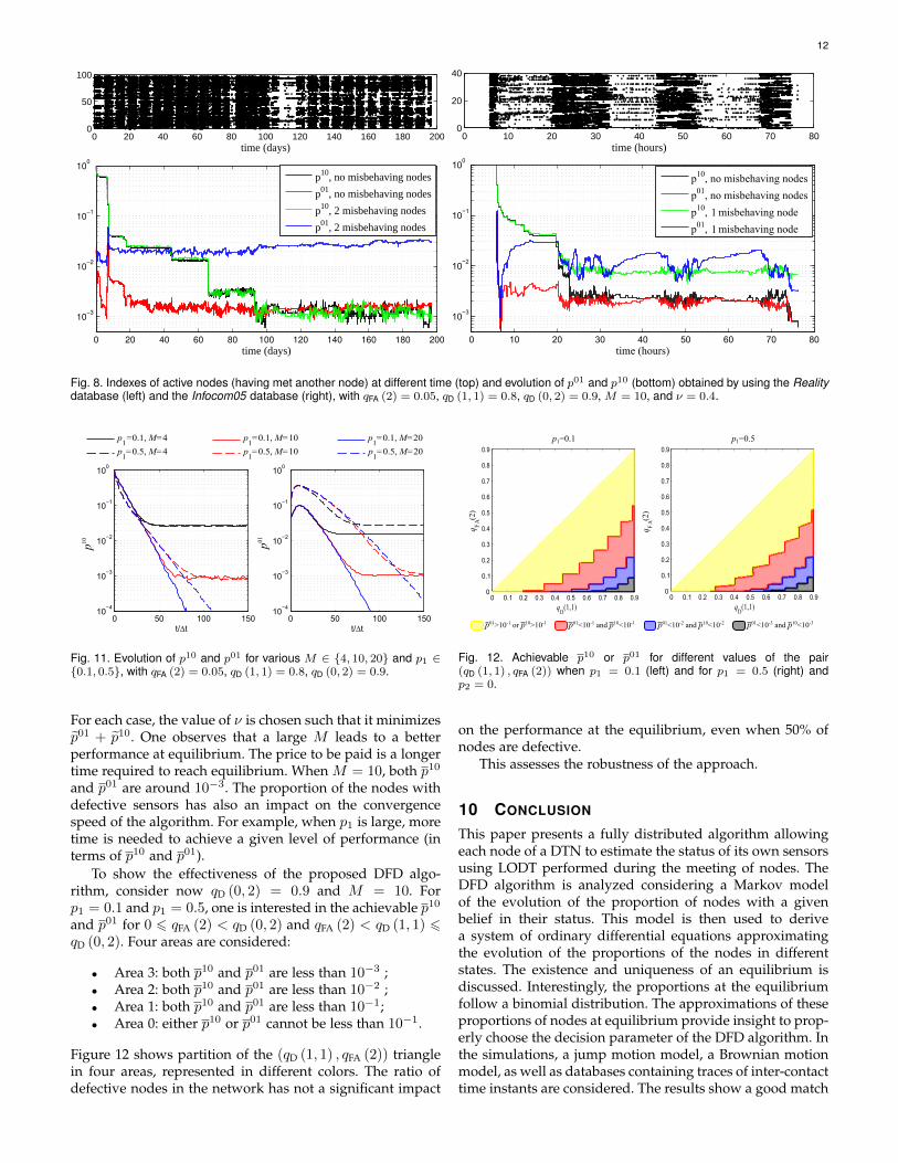
Consider again the following parameters: qFA (2) = 0.05,qD (1, 1) = 0.8, qD (0, 2) = 0.9, M = 10, and ν = 0.4.Monte-Carlo simulations are performed 500 times for eachdatabase. In each test, n1 nodes with random index arechosen to be defective. One sets n1 = 10 in Infocom05 andn1 = 20 in Reality. Two cases are considered. First, nomisbehaving node is introduced, i.e., n2 = 0. In a secondcase, n2 = 1 in Infocom05 and n2 = 2 in Reality. At thetop of Figure 8, the index of the active nodes (which havecontact with the others) are presented at each time to showthe frequency of the inter-contacts at different epochs. Theevolution of p10 and p01 is plotted at the bottom of Figure 8.Interestingly, in absence of misbehaving nodes, both p10 andp01, obtained with both databases, decrease to 10−3 after asufficiently long time. One also observes that the conver-gence speed of p10 and p01 is highly related to the inter-contact rate (reflected by the density of points in the sub-figures at the top). Considering Infocom05, Table 2 furthershows the influence of misbehaving nodes for various n2.In presence of misbehaving nodes, the performance of theDFD algorithms worsens, but remains satisfying if the valueof ν is properly chosen.
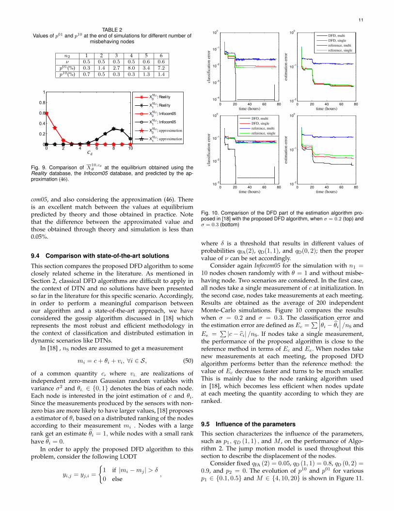
When n2 = 0, Figure 9 represents the states at equilib-rium X
M,cd
θ obtained with the databases Reality and Info-
11
TABLE 2Values of p01 and p10 at the end of simulations for different number of
misbehaving nodes
n2 1 2 3 4 5 6ν 0.5 0.5 0.5 0.5 0.6 0.6
p01(%) 0.3 1.4 2.7 8.0 3.4 7.2p10(%) 0.7 0.5 0.3 0.3 1.3 1.4
0 2 4 6 8 100
0.2
0.4
0.6
0.8
1
cd
X010,cd, Reality
X110,cd, Reality
X010,cd, Infocom05
X110,cd, Infocom05
X010,cd, approximation
X110,cd, approximation
Fig. 9. Comparison of X10,cdθ at the equilibrium obtained using the
Reality database, the Infocom05 database, and predicted by the ap-proximation (46).
com05, and also considering the approximation (46). Thereis an excellent match between the values at equilibriumpredicted by theory and those obtained in practice. Notethat the difference between the approximated value andthose obtained through theory and simulation is less than0.05%.
9.4 Comparison with state-of-the-art solutions
This section compares the proposed DFD algorithm to someclosely related scheme in the literature. As mentioned inSection 2, classical DFD algorithms are difficult to apply inthe context of DTN and no solutions have been presentedso far in the literature for this specific scenario. Accordingly,in order to perform a meaningful comparison betweenour algorithm and a state-of-the-art approach, we haveconsidered the gossip algorithm discussed in [18] whichrepresents the most robust and efficient methodology inthe context of classification and distributed estimation indynamic scenarios like DTNs.
In [18] , nS nodes are assumed to get a measurement
mi = c+ θi + vi, ∀i ∈ S, (50)
of a common quantity c, where vi. are realizations ofindependent zero-mean Gaussian random variables withvariance σ2 and θi. ∈ {0, 1} denotes the bias of each node.Each node is interested in the joint estimation of c and θi.Since the measurements produced by the sensors with non-zero bias are more likely to have larger values, [18] proposesa estimator of θi based on a distributed ranking of the nodesaccording to their measurement mi . Nodes with a largerank get an estimate θi = 1, while nodes with a small rankhave θi = 0.
In order to apply the proposed DFD algorithm to thisproblem, consider the following LODT
yi,j = yj,i =
{1 if |mi −mj | > δ
0 else,
0 20 40 60 80
10−4
10−3
10−2
10−1
100
time (hours)
clas
sifi
cati
on
err
or
0 20 40 60 8010
−2
10−1
100
time (hours)
esti
mat
ion
err
or
DFD, multi
DFD, single
reference, multi
reference, single
0 20 40 60 8010
−3
10−2
10−1
100
time (hours)
clas
sifi
cati
on
err
or
0 20 40 60 8010
−2
10−1
100
time (hours)
esti
mat
ion
err
or
DFD, multi
DFD, single
reference, multi
reference, single
Fig. 10. Comparison of the DFD part of the estimation algorithm pro-posed in [18] with the proposed DFD algorithm, when σ = 0.2 (top) andσ = 0.3 (bottom)
where δ is a threshold that results in different values ofprobabilities qFA(2), qD(1, 1), and qD(0, 2); then the propervalue of ν can be set accordingly.
Consider again Infocom05 for the simulation with n1 =10 nodes chosen randomly with θ = 1 and without misbe-having node. Two scenarios are considered. In the first case,all nodes take a single measurement of c at initialization. Inthe second case, nodes take measurements at each meeting.Results are obtained as the average of 200 independentMonte-Carlo simulations. Figure 10 compares the resultswhen σ = 0.2 and σ = 0.3. The classification error andthe estimation error are defined as Ec =
∑∣∣∣θi − θi∣∣∣ /nS andEe =
∑|c− ci| /nS. If nodes take a single measurement,
the performance of the proposed algorithm is close to thereference method in terms of Ec and Ee. When nodes takenew measurements at each meeting, the proposed DFDalgorithm performs better than the reference method: thevalue of Ec decreases faster and turns to be much smaller.This is mainly due to the node ranking algorithm usedin [18], which becomes less efficient when nodes updateat each meeting the quantity according to which they areranked.
9.5 Influence of the parametersThis section characterizes the influence of the parameters,such as p1, qD (1, 1) , and M , on the performance of Algo-rithm 2. The jump motion model is used throughout thissection to describe the displacement of the nodes.
Consider fixed qFA (2) = 0.05, qD (1, 1) = 0.8, qD (0, 2) =0.9, and p2 = 0. The evolution of p10 and p01 for variousp1 ∈ {0.1, 0.5} and M ∈ {4, 10, 20} is shown in Figure 11.
12
0 20 40 60 80 100 120 140 160 180 2000
50
100
time (days)0 10 20 30 40 50 60 70 80
0
20
40
time (hours)
0 20 40 60 80 100 120 140 160 180 200
10−3
10−2
10−1
100
time (days)
p10
, no misbehaving nodes
p01
, no misbehaving nodes
p10
, 2 misbehaving nodes
p01
, 2 misbehaving nodes
0 10 20 30 40 50 60 70 80
10−3
10−2
10−1
100
time (hours)
p10, no misbehaving nodes
p01, no misbehaving nodes
p10, misbehaving node
p01, misbehaving node1
1
Fig. 8. Indexes of active nodes (having met another node) at different time (top) and evolution of p01 and p10 (bottom) obtained by using the Realitydatabase (left) and the Infocom05 database (right), with qFA (2) = 0.05, qD (1, 1) = 0.8, qD (0, 2) = 0.9, M = 10, and ν = 0.4.
p1=0.1, M=10 p
1=0.1, M=20
p1=0.5, M=4 p
1=0.5, M=10 p
1=0.5, M=20
p1=0.1, M=4
0 50 100 15010
−4
10−3
10−2
10−1
100
p10
t/∆t0 50 100 150
10−4
10−3
10−2
10−1
100
p01
t/∆t
Fig. 11. Evolution of p10 and p01 for various M ∈ {4, 10, 20} and p1 ∈{0.1, 0.5}, with qFA (2) = 0.05, qD (1, 1) = 0.8, qD (0, 2) = 0.9.
For each case, the value of ν is chosen such that it minimizesp01 + p10. One observes that a large M leads to a betterperformance at equilibrium. The price to be paid is a longertime required to reach equilibrium. When M = 10, both p10
and p01 are around 10−3. The proportion of the nodes withdefective sensors has also an impact on the convergencespeed of the algorithm. For example, when p1 is large, moretime is needed to achieve a given level of performance (interms of p10 and p01).
To show the effectiveness of the proposed DFD algo-rithm, consider now qD (0, 2) = 0.9 and M = 10. Forp1 = 0.1 and p1 = 0.5, one is interested in the achievable p10
and p01 for 0 6 qFA (2) < qD (0, 2) and qFA (2) < qD (1, 1) 6qD (0, 2). Four areas are considered:
• Area 3: both p10 and p01 are less than 10−3 ;• Area 2: both p10 and p01 are less than 10−2 ;• Area 1: both p10 and p01 are less than 10−1;• Area 0: either p10 or p01 cannot be less than 10−1.
Figure 12 shows partition of the (qD (1, 1) , qFA (2)) trianglein four areas, represented in different colors. The ratio ofdefective nodes in the network has not a significant impact
0 0.1 0.2 0.3 0.4 0.5 0.6 0.7 0.8 0.90
0.1
0.2
0.3
0.4
0.5
0.6
0.7
0.8
0.9
qD
(1,1)
qF
A(2
)
qF
A(2
)
0 0.1 0.2 0.3 0.4 0.5 0.6 0.7 0.8 0.90
0.1
0.2
0.3
0.4
0.5
0.6
0.7
0.8
0.9
qD
(1,1)
p01>10-1 or p10>10-1 p01<10-1 and p10<10-1 p01<10-2 and p10<10-2 p01<10-3 and p10<10-3
p1=0.1 p1=0.5
Fig. 12. Achievable p10 or p01 for different values of the pair(qD (1, 1) , qFA (2)) when p1 = 0.1 (left) and for p1 = 0.5 (right) andp2 = 0.
on the performance at the equilibrium, even when 50% ofnodes are defective.
This assesses the robustness of the approach.
10 CONCLUSION
This paper presents a fully distributed algorithm allowingeach node of a DTN to estimate the status of its own sensorsusing LODT performed during the meeting of nodes. TheDFD algorithm is analyzed considering a Markov modelof the evolution of the proportion of nodes with a givenbelief in their status. This model is then used to derivea system of ordinary differential equations approximatingthe evolution of the proportions of the nodes in differentstates. The existence and uniqueness of an equilibrium isdiscussed. Interestingly, the proportions at the equilibriumfollow a binomial distribution. The approximations of theseproportions of nodes at equilibrium provide insight to prop-erly choose the decision parameter of the DFD algorithm. Inthe simulations, a jump motion model, a Brownian motionmodel, as well as databases containing traces of inter-contacttime instants are considered. The results show a good match
13
with theory. The convergence speed of the DFD algorithmdepends on the inter-contact rate and on the proportion ofnodes with defective sensors p1. Nevertheless, p1 has nota significant impact on the non-detection and false alarmrates at equilibrium, showing the robustness of the approachalso in case of a large number of defective nodes. Theimpact of the presence of misbehaving nodes has also beenconsidered, showing the robustness of the proposed DFDalgorithm.
REFERENCES
[1] M. J. Khabbaz, C. M. Assi, and W. F. Fawaz, “Disruption-tolerantnetworking: A comprehensive survey on recent developments andpersisting challenges,” IEEE Com. Surv. & Tut., vol. 14, no. 2, pp.607–640, 2012.
[2] P. R. Pereira, A. Casaca, J. J. Rodrigues, V. N. Soares, J. Triay, andC. Cervello-Pastor, “From delay-tolerant networks to vehiculardelay-tolerant networks,” IEEE Com. Surv. & Tut., vol. 14, no. 4,pp. 1166–1182, 2012.
[3] K. Wei, M. Dong, J. Weng, G. Shi, K. Ota, and K. Xu, “Congestion-aware message forwarding in delay tolerant networks: acommunity perspective,” Concurrency and Computation: Practiceand Experience, vol. 27, no. 18, pp. 5722–5734, 2015.
[4] P. Hui, J. Crowcroft, and E. Yoneki, “Bubble rap: Social-basedforwarding in delay-tolerant networks,” IEEE Trans. Mob. Comp.,vol. 10, no. 11, pp. 1576–1589, 2011.
[5] V. N. Soares, J. J. Rodrigues, and F. Farahmand, “Geospray: A ge-ographic routing protocol for vehicular delay-tolerant networks,”Information Fusion, vol. 15, pp. 102–113, 2014.
[6] H. Zhu, S. Du, Z. Gao, M. Dong, and Z. Cao, “A probabilisticmisbehavior detection scheme toward efficient trust establishmentin delay-tolerant networks,” IEEE Trans. Paral. and Dist. Syst.,vol. 25, no. 1, pp. 22–32, 2014.
[7] L. Galluccio, B. Lorenzo, and S. Glisic, “Sociality-aided new adap-tive infection recovery schemes for multicast dtns,” IEEE Trans.Veh. Tech., vol. 65, no. 5, pp. 3360–3376, 2016.
[8] M. Panda, A. Ali, T. Chahed, and E. Altman, “Tracking messagespread in mobile delay tolerant networks,” IEEE Trans. Mob.Comp., vol. 14, no. 8, pp. 1737–1750, 2015.
[9] W. Li, F. Bassi, D. Dardari, M. Kieffer, and G. Pasolini, “Defectivesensor identification for WSNs involving generic local outlierdetection tests,” IEEE Trans. Sig. and Inf. Proc. over Netw., vol. 2,no. 1, pp. 29–48, 2016.
[10] J. Chen, S. Kher, and A. Somani, “Distributed fault detection ofwireless sensor networks,” in Proc. DIWANS, New York, NY, 2006,pp. 65 – 72.
[11] J.-L. Gao, Y.-J. Xu, and X.-W. Li, “Weighted-median based dis-tributed fault detection for wireless sensor networks,” Jnl of Softw.,vol. 18, no. 5, pp. 1208 – 1217, 2007.
[12] S. Ji, S.-F. Yuan, T.-H. Ma, and C. Tan, “Distributed fault detectionfor wireless sensor based on weighted average,” in Proc NSWCTC,Wuhan, China, 2010, pp. 57 – 60.
[13] M. Panda and P. Khilar, “Distributed self fault diagnosis algorithmfor large scale wireless sensor networks using modified threesigma edit test,” Ad Hoc Networks, vol. 25, pp. 170–184, 2015.
[14] Y. Zhang, N. Meratnia, and P. Havinga, “Outlier detection tech-niques for wireless sensor networks: A survey,” IEEE Com. Surv.& Tut., vol. 12, no. 2, pp. 159–170, 2010.
[15] A. Mahapatro and P. M. Khilar, “Fault diagnosis in wireless sensornetworks: A survey,” IEEE Com. Surv. & Tut., vol. 15, no. 4, pp.2000–2026, 2013.
[16] H. Dong, Z. Wang, S. X. Ding, and H. Gao, “A survey on dis-tributed filtering and fault detection for sensor networks,” Math.Prob. in Eng., 2014.
[17] E. F. Nakamura, A. A. Loureiro, and A. C. Frery, “Informationfusion for wireless sensor networks: Methods, models, and classi-fications,” ACM Comp. Surv., vol. 39, no. 3, p. 9, 2007.
[18] A. Chiuso, F. Fagnani, L. Schenato, and S. Zampieri, “Gossip algo-rithms for simultaneous distributed estimation and classificationin sensor networks,” IEEE Jnl Sel. Top. Sig. Proc., vol. 5, no. 4, pp.691–706, 2011.
[19] F. Fagnani, S. M. Fosson, and C. Ravazzi, “A distributed classifica-tion/estimation algorithm for sensor networks,” SIAM Jnl Contr.and Opt., vol. 52, no. 1, pp. 189–218, 2014.
[20] ——, “Consensus-like algorithms for estimation of gaussian mix-tures over large scale networks,” Math. Mod. and Meth. in App.Sciences, vol. 24, no. 02, pp. 381–404, 2014.
[21] B. Zhu, W. Zhang, W. Feng, and L. Zhang, “Distributed faultynode detection and isolation in delay-tolerant vehicular sensornetworks,” in Proc. PIMRC, Sept 2012, pp. 1497–1502.
[22] W. Peng, F. Li, X. Zou, and J. Wu, “Behavioral malware detectionin delay tolerant networks,” IEEE Trans. on Paral. and Dist. Syst.,vol. 25, no. 1, pp. 53–63, 2014.
[23] E. Hernandez-Orallo, M. D. Serrat Olmos, J.-C. Cano, C. T.Calafate, and P. Manzoni, “Cocowa: A collaborative contact-basedwatchdog for detecting selfish nodes,” IEEE Trans. Mob. Comp.,vol. 14, no. 6, pp. 1162–1175, 2015.
[24] E. Ayday and F. Fekri, “An iterative algorithm for trust manage-ment and adversary detection for delay-tolerant networks,” IEEETrans. Mob. Comp., vol. 11, no. 9, pp. 1514–1531, 2012.
[25] Y. Liu, D. R. Bild, R. P. Dick, Z. M. Mao, and D. S. Wallach, “Themason test: A defense against sybil attacks in wireless networkswithout trusted authorities,” IEEE Trans. Mob. Comp., vol. 14,no. 11, pp. 2376–2391, 2015.
[26] J. R. Douceur, “The sybil attack,” in Peer-to-peer Systems. Springer,2002, pp. 251–260.
[27] G. Han, J. Jiang, L. Shu, and M. Guizani, “An attack-resistant trustmodel based on multidimensional trust metrics in underwateracoustic sensor network,” IEEE Trans. Mob. Comp., vol. 14, no. 12,pp. 2447–2459, 2015.
[28] M. Abdelhakim, L. E. Lightfoot, J. Ren, and T. Li, “Distributed de-tection in mobile access wireless sensor networks under byzantineattacks,” IEEE Trans. on Paral. and Dist. Syst., vol. 25, no. 4, pp.950–959, 2014.
[29] H. Zhu, L. Fu, G. Xue, Y. Zhu, M. Li, and L. Ni, “Recognizingexponential inter-contact time in vanets,” in Proc. INFOCOM,March 2010, pp. 1–5.
[30] J. P. Norton, Ed., Special Issue on Bounded-Error Estimation:Issue 1, 1994, Int. Jnl Adapt. Cont. Sig. Proc. 8(1):1–118.
[31] ——, Special Issue on Bounded-Error Estimation: Issue 2, 1995,Int. Jnl Adapt. Cont. Sig. Proc. 9(1):1–132.
[32] M. Milanese, J. Norton, H. Piet-Lahanier, and E. Walter, Eds.,Bounding Approaches to System Identification. New York, NY:Plenum Press, 1996.
[33] A. Shwartz and A. Weiss, “Large deviations for performanceanalysis,” 1995.
[34] T. G. Kurtz, “The central limit theorem for markov chains,” TheAnnals of Prob., pp. 557–560, 1981.
[35] W. O. Kermack and A. G. McKendrick, “A contribution to themathematical theory of epidemics,” in Proc. Royal Soc. London, Ser.A, vol. 115, no. 772, 1927, pp. 700–721.
[36] Z. J. Haas and T. Small, “A new networking model for biologicalapplications of ad hoc sensor networks,” IEEE/ACM Trans. Netw.,vol. 14, no. 1, pp. 27–40, 2006.
[37] E. Renshaw, Modelling biological populations in space and time. Cam-bridge University Press, 1993, vol. 11.
[38] M. E. Newman, “Spread of epidemic disease on networks,” Phys.Rev. E, vol. 66, no. 1, July 2002.
[39] T. Spyropoulos, T. Turletti, and K. Obraczka, “Routing in delay-tolerant networks comprising heterogeneous node populations,”IEEE Trans. Mob. Comp., vol. 8, no. 8, pp. 1132–1147, 2009.
[40] Y. Lin, B. Li, and B. Liang, “Stochastic analysis of network codingin epidemic routing,” IEEE Jnl Sel. Ar. Com., vol. 26, no. 5, 2008.
[41] A. Granas and J. Dugundji, Fixed point theory. Springer, 2013.[42] S. Banach, “Sur les operations dans les ensembles abstraits et leur
application aux equations integrales,” Fund. Math., vol. 3, no. 1,pp. 133–181, 1922.
[43] N. Eagle and A. Pentland, “Reality mining: sensing complex socialsystems,” Pers. Ubiq. Comp., vol. 10, no. 4, pp. 255–268, 2006.
[44] J. Scott, R. Gass, J. Crowcroft, P. Hui, C. Diot, and A. Chaintreau,“CRAWDAD dataset cambridge/haggle (v. 2009-05-29),” Down-loaded from http://crawdad.org/cambridge/haggle/20090529,May 2009.
[45] M. Orlinski, “Encounter traces for the one simulator,” Down-loaded from http://www.shigs.co.uk/index.php?page=traces.
[46] T. M. Cover and J. A. Thomas, Elements of information theory. JohnWiley & Sons, 2012.

14
Wenjie Li received the B.S. degree from theHuazhong University of Science and Technol-ogy, China, in 2011, and the M.S. degree inAdvanced Systems of Wireless Communicationfrom the University of Paris-Sud, France, in2013. He is currently pursuing the Ph.D. degreeat the Laboratoire des Signaux et Systemes,France. He has been visiting Ph.D. student atthe University of Bologna, Italy, in 2014 and2015. His research interests lie in the areas ofdistributed signal processing over networks and
information theory.
Laura Galluccio received her laurea degree inElectrical Engineering from University of Cata-nia, Catania, Italy, in 2001. In March 2005she got her Ph.D. in Electrical, Computer andTelecommunications Engineering at the sameuniversity. Since 2002 she is also at the Ital-ian National Consortium of Telecommunications(CNIT), where she worked as a Research Fel-low within the VICOM (Virtual Immersive Com-munications) and the SATNEX Projects. SinceNovember 2010 she is Assistant Professor at
University of Catania. Her research interests include ad hoc and sensornetworks, protocols and algorithms for wireless networks, and networkperformance analysis. From May to July 2005 she has been a VisitingScholar at the COMET Group, Columbia University, NY. In Septem-ber 2015 she has been Visiting Professor at CentraleSupelec, Gif-sur-Yvette, France. She is member of the IEEE, Comsoc and ACMN2Women Group.
Francesca Bassi received the Master of Sci-ence degree in telecommunications engineeringfrom the University of Bologna, Bologna, Italy,in 2006, and the Ph.D. degree from UniversityParis-Sud, Orsay, France, and from the Univer-sity of Bologna, in 2010. In 2007 and 2009, shehas been a visiting Ph.D. student at the Univer-sity of Bologna. From 2006 to 2010, she waswith Laboratoire des Signaux et des Systemes,Gif-sur-Yvette, France. Between 2011 and 2012,she was a Postdoctoral Researcher at the Uni-
versity of Michigan, Ann Arbor, MI, USA. Since 2012, she has been anAssistant Professor at ESME-Sudria, Ivry-sur-Seine, France, and an As-sociate Researcher with the Laboratoire des Signaux et des Systemes.
Michel Kieffer is a full professor in signal pro-cessing for communications at the Paris-SudUniversity and a researcher at the Laboratoiredes Signaux et Systemes, Gif-sur-Yvette. Since2009, he is also part-time invited professorat the Laboratoire Traitement et Communica-tion de l’Information, Telecom ParisTech, Paris.His research interests are in signal processingfor multimedia, communications, and network-ing, distributed source coding, network coding,joint source-channel coding and decoding, joint
source-network coding. Michel Kieffer is co-author of more than 150contributions in journals, conference proceedings, or books. He is oneof the co-authors of the book Applied Interval Analysis published bySpringer-Verlag in 2001, and of the book Joint source-channel decod-ing: A crosslayer perspective with applications in video broadcastingpublished by Academic Press in 2009. He serves as associate editorof Signal Processing since 2008 and of the IEEE Transactions onCommunications from 2012 to 2016. From 2011 to 2016, Michel Kiefferwas junior member of the Institut Universitaire de France.
15
𝜋𝜃1,0 𝜋𝜃
1,1
𝜃, 𝑐𝑚 + 1, 𝑐𝑑 + 1 𝜃, 𝑐𝑚 + 1, 𝑐𝑑
𝜃, 𝑐𝑚 , 𝑐𝑑
𝜃, 𝑐𝑚 − 1, 𝑐𝑑 𝜃, 𝑐𝑚 − 1, 𝑐𝑑 − 1
𝜋𝜃1,0 𝜋𝜃
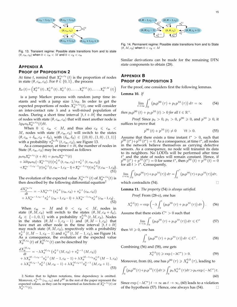
1,1 𝜋𝜃0,0
Fig. 13. Transient regime: Possible state transitions from and to state(θ, cm, cd) when 0 < cm < M and 0 < cd < cm
APPENDIX APROOF OF PROPOSITION 2At time t, remind that Xcm,cd
θ (t) is the proportion of nodesin state (θ, cm, cd). For θ ∈ {0, 1} , the process
Xθ (t)=(X0,0θ (t) ,X1,0
θ (t) ,X1,1θ (t) , . . . ,XM,0θ (t) , . . . ,XM,Mθ (t)
)is a jump Markov process with random jump time in-
stants and with a jump size 1/nθ . In order to get theexpected proportions of nodes Xcm,cd
θ (t), one will consideran inter-contact rate λ and a well-mixed population ofnodes. During a short time interval [t, t+ δt] the numberof nodes with state (θ, cm, cd) that will meet another node isλpθnSX
cm,cdθ (t)δt.
When 0 6 cm < M , and thus also cd 6 cm <M , nodes with state (θ, cm, cd) will switch to the states(θ, cm + δm, cd + δd), with (δm, δd) ∈ {(0, 0) , (1, 0) , (1, 1)}with a probability πδm,δd
θ (t, cm, cd), see Figure 13.As a consequence, at time t+ δt, the number of nodes in
State (θ, cm, cd) may be expressed as follows
pθnSXcm,cdθ (t+ δt) = pθnSX
cm,cdθ (t)
+ λδtpθnS(−Xcm,cd
θ (t)(π1,0θ (t, cm, cd)+π1,1
θ (t, cm, cd))
+Xcm−1,cd−1θ (t)π1,1
θ (t, cm−1,cd−1)+Xcm−1,cdθ (t)π1,0
θ (t,cm−1,cd)).
(51)
The evolution of the expected value Xcm,cdθ (t) of Xcm,cd
θ (t) isthen described by the following differential equation2
dXcm,cdθ
dt= −λXcm,cd
θ
(π1,0θ (cm, cd) + π1,1
θ (cm, cd))
+ λXcm−1,cd−1θ π1,1
θ (cm−1,cd−1) + λXcm−1,cdθ π1,0
θ (cm−1,cd) .(52)
When cm = M and 0 < cd < M , nodes instate (θ,M, cd) will switch to the states (θ,M, cd + δd),δd ∈ {−1, 0, 1} with a probability π0,δd
θ (t,M, cd). Nodesin the states (θ,M − 1, cd − 1) and (θ,M − 1, cd) thathave met an other node in the time interval [t, t+ δt]may reach state (θ,M, cd), respectively with a probabilityπ1,1θ (t,M − 1, cd − 1) and π1,0
θ (t,M − 1, cd), see Figure 14.As a consequence, the evolution of the expected valueXM,cdθ (t) of XM,cd
θ (t) can be described by
dXM,cdθ
dt= −λXM,cd
θ
(π0,1θ (M, cd) + π0,−1
θ (M, cd))
+ λXM−1,cd−1θ π1,1
θ (M − 1, cd − 1) + λXM−1,cdθ π1,0
θ (M − 1, cd)
+ λXM,cd−1θ π0,1
θ (M, cd − 1) + λXM,cd+1θ π0,−1
θ (M, cd + 1) .(53)
2. Notice that to lighten notations, time dependency is omitted.Moreover, πδm,δd
θ (cm, cd) and pθθ in the rest of the paper represent theexpected values, as they can be represented as functions of Xcm,cd
θ (t) orXcm,cdθ (t).
𝜋𝜃0,−1
𝜋𝜃0,−1
𝜃,𝑀, 𝑐𝑑 + 1 𝜃,𝑀, 𝑐𝑑 − 1 𝜃,𝑀, 𝑐𝑑
𝜃,𝑀 − 1, 𝑐𝑑 𝜃,𝑀 − 1, 𝑐𝑑 − 1
𝜋𝜃1,0
𝜋𝜃1,1
𝜋𝜃0,0
𝜋𝜃0,1
𝜋𝜃0,1
Fig. 14. Permanent regime: Possible state transitions from and to State(θ,M, cd) when 0 < cd < M
Similar derivations can be made for the remaining DTNstate components to obtain (28).
APPENDIX BPROOF OF PROPOSITION 3For the proof, one considers first the following lemmas.
Lemma 10. If
limt→∞
ˆ t
0
(p0p
00 (τ) + p1p10 (τ)
)dτ =∞ (54)
then p0p00 (t) + p1p10 (t) > 0 for all t ∈ R+.
Proof: Since p0 > 0, p1 > 0, p00 > 0, and p10 > 0, itsuffices to prove that
p00 (t) + p10 (t) 6= 0 ∀t > 0. (55)
Assume that there exists a time instant t∗ > 0, such thatp00 (t∗)+p10 (t∗) = 0. As a consequence, at time t∗, all nodesin the network believe themselves as carrying defectivesensors. As a consequence, no node will transmit its datato its neighbors. No LODTs will be performed after timet∗ and the state of nodes will remain constant. Hence, ifp00 (t∗) + p10 (t∗) = 0 for some t∗, then p00 (t) + p10 (t) = 0for all t > t∗. Consequently,
limt→∞
ˆ t
0
(p0p
00(τ)+p1p10(τ)
)dτ =
ˆ t∗
0
(p0p
00(τ)+p1p10(τ)
)dτ,
which contradicts (54).
Lemma 11. The property (54) is always satisfied.
Proof: From (28-a), one has
X0,0θ (t) = exp
(−λˆ t
0
(p0p
00 (τ) + p1p10 (τ)
)dτ
). (56)
Assume that there exists C∗ > 0 such that
limt→∞
ˆ t
0
(p0p
00 (τ) + p1p10 (τ)
)dτ 6 C∗ (57)
then ∀t > 0, one hasˆ t
0
(p0p
00 (τ) + p1p10 (τ)
)dτ 6 C∗. (58)
Combining (56) and (58), one gets
X0,0θ (t) > exp (−λC∗) > 0. (59)
Moreover, from (6), one has p00 (τ) > X0,0θ (τ), leading to
ˆ t
0
(p0p
00(τ)+p1p10(τ)
)dτ>
ˆ t
0
p0X0,0θ (τ)dτ >p0 exp (−λC∗) t.
(60)
Since exp (−λC∗) t→∞ as t→∞, (60) leads to a violationof the hypothesis (57). Hence, one always has (54).
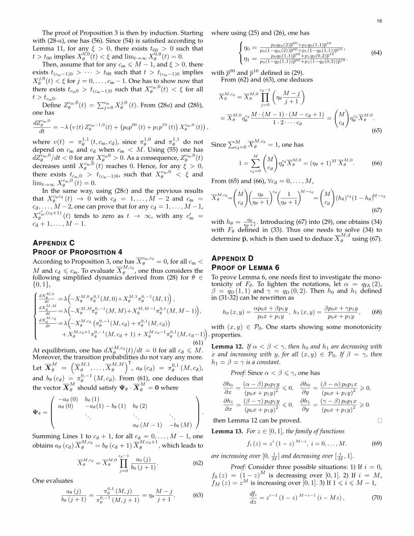
16
The proof of Proposition 3 is then by induction. Startingwith (28-a), one has (56). Since (54) is satisfied according toLemma 11, for any ξ > 0, there exists t00 > 0 such thatt > t00 implies X0,0
θ (t) < ξ and limt→∞X0,0θ (t) = 0.
Then, assume that for any cm 6M − 1, and ξ > 0, thereexists t(cm−1)0 > · · · > t00 such that t > t(cm−1)0 impliesXj,0θ (t) < ξ for j = 0, . . . , cm−1. One has to show now that
there exists tcm0 > t(cm−1)0 such that Xcm,0θ (t) < ξ for all
t > tcm0.Define Zcm,0
θ (t) =∑cmj=0X
j,0θ (t). From (28a) and (28b),
one has
dZcm,0θ
dt= −λ
(v (t)Zcm−1,0
θ (t) +(p0p
00 (t) + p1p10 (t)
)Xcm,0θ (t)
),
where v(t) = π1,1θ (t, cm, cd), since π1,0
θ and π1,1θ do not
depend on cm and cd when cm < M . Using (55) one hasdZcm,0
θ /dt < 0 for any Xcm0θ > 0. As a consequence, Zcm,0
θ (t)decreases until Xcm,0
θ (t) reaches 0. Hence, for any ξ > 0,there exists tcm,0 > t(cm−1)0, such that Xcm,0
θ < ξ andlimt→∞ Xcm,0
θ (t) = 0.In the same way, using (28c) and the previous results
that Xcmcdθ (t) → 0 with cd = 1, . . . ,M − 2 and cm =
cd, . . . ,M −2, one can prove that for any cd = 1, . . . ,M −1,Xc′m,(cd+1)θ (t) tends to zero as t → ∞, with any c′m =
cd + 1, . . . ,M − 1.
APPENDIX CPROOF OF PROPOSITION 4According to Proposition 3, one has X
cm,cd
θ = 0, for all cm <
M and cd 6 cm. To evaluate XM,cd
θ , one thus considers thefollowing simplified dynamics derived from (28) for θ ∈{0, 1},
dXM,0θdt
=λ(−XM,0
θ π0,1θ (M, 0)+XM,1
θ π0,−1θ (M, 1)
),
dXM,Mθdt
=λ(−XM,M
θ π0,−1θ (M,M)+XM,M−1
θ π0,1θ (M,M− 1)
),
dXM,cdθdt
=λ(−XM,cd
θ
(π0,−1θ (M, cd) + π0,1
θ (M, cd))
+XM,cd+1θ π0,−1
θ (M, cd + 1) +XM,cd−1θ π0,1
θ (M, cd−1)).
(61)At equilibrium, one has dXM,cd
θ (t)/dt = 0 for all cd 6 M .Moreover, the transition probabilities do not vary any more.
Let XM
θ =(XM,1θ , . . . , X
M,Mθ
)T, aθ (cd) = π0,1
θ (M, cd),
and bθ (cd) = π0,−1θ (M, cd). From (61), one deduces that
the vector XM
θ should satisfy Ψθ ·XM
θ = 0 where
Ψθ =
−aθ (0) bθ (1)aθ (0) −aθ(1)− bθ (1) bθ (2)
. . .. . .
. . .aθ (M − 1) −bθ (M)
.
Summing Lines 1 to cd + 1, for all cd = 0, . . . ,M − 1, oneobtains aθ (cd)X
M,cd
θ = bθ (cd + 1)XM,cd+1θ , which leads to
XM,cdθ = X
M,0θ
cd−1∏j=0
a0 (j)
b0 (j + 1). (62)
One evaluates
aθ (j)
bθ (j + 1)=
π0,1θ (M, j)
π0,−1θ (M, j + 1)
= ηθM − jj + 1
, (63)
where using (25) and (26), one hasη0 = p0qFA(2)p00+p1qD(1,1)p
10
p0(1−qFA(2))p00+p1(1−qD(1,1))p10,
η1 = p0qD(1,1)p00+p1qD(0,2)p
10
p0(1−qD(1,1))p00+p1(1−qD(0,2))p10.
(64)
with p00 and p10 defined in (29).From (62) and (63), one deduces
XM,cdθ = X
M,0θ
cd−1∏j=0
(ηθM − jj + 1
)
= XM,0θ ηcd
θ
M · (M − 1) · (M − cd + 1)
1 · 2 · · · · cd=
(M
cd
)ηcdθ X
M,0θ .
(65)
Since∑Mcd=0X
M,cd
θ = 1, one has
1 =
M∑cd=0
(M
cd
)ηcdθ X
M,0θ = (ηθ + 1)M X
M,0θ . (66)
From (65) and (66), ∀cd = 0, . . . ,M ,
XM,cdθ =
(M
cd
)(ηθ
ηθ + 1
)cd(
1
ηθ + 1
)M−cd
=
(M
cd
)(hθ)
cd (1− hθ)M−cd
(67)
with hθ = ηθηθ+1 . Introducing (67) into (29), one obtains (34)
with Fθ defined in (33). Thus one needs to solve (34) todetermine p, which is then used to deduce X
M,dθ using (67).
APPENDIX DPROOF OF LEMMA 6To prove Lemma 6, one needs first to investigate the mono-tonicity of Fθ . To lighten the notations, let α = qFA (2),β = qD (1, 1) and γ = qD (0, 2). Then h0 and h1 definedin (31-32) can be rewritten as
h0 (x, y) =αp0x+ βp1y
p0x+ p1y, h1 (x, y) =
βp0x+ γp1y
p0x+ p1y, (68)
with (x, y) ∈ P0. One starts showing some monotonicityproperties.
Lemma 12. If α < β < γ, then h0 and h1 are decreasing withx and increasing with y, for all (x, y) ∈ P0. If β = γ, thenh1 = β = γ is a constant.
Proof: Since α < β 6 γ, one has
∂h0
∂x=
(α− β) p0p1y
(p0x+ p1y)26 0,
∂h0
∂y=
(β − α) p0p1x
(p0x+ p1y)2> 0,
∂h1
∂x=
(β − γ) p0p1y
(p0x+ p1y)26 0,
∂h1
∂y=
(γ − β) p0p1x
(p0x+ p1y)2> 0.
then Lemma 12 can be proved.
Lemma 13. For z ∈ [0, 1], the family of functions
fi (z) = zi (1− z)M−i, i = 0, . . . ,M. (69)
are increasing over [0, iM ] and decreasing over [ iM , 1].
Proof: Consider three possible situations: 1) If i = 0,f0 (z) = (1− z)M is decreasing over [0, 1]. 2) If i = M ,fM (z) = zM is increasing over [0, 1]. 3) If 1 6 i 6M − 1,
dfidz
= zi−1 (1− z)M−i−1 (i−Mz) , (70)
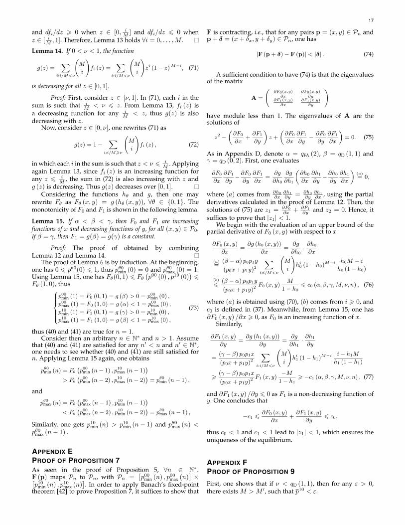
17
and dfi/dz > 0 when z ∈ [0, iM ] and dfi/dz 6 0 when
z ∈ [ iM , 1]. Therefore, Lemma 13 holds ∀i = 0, . . . ,M.
Lemma 14. If 0 < ν < 1, the function
g(z) =∑
i:i/M<ν
(M
i
)fi (z) =
∑i:i/M<ν
(M
i
)zi (1− z)M−i, (71)
is decreasing for all z ∈ [0, 1].
Proof: First, consider z ∈ [ν, 1]. In (71), each i in thesum is such that i
M < ν 6 z. From Lemma 13, fi (z) isa decreasing function for any i
M < z, thus g(z) is alsodecreasing with z.
Now, consider z ∈ [0, ν], one rewrites (71) as
g(z) = 1−∑
i:i/M>ν
(M
i
)fi (z) , (72)
in which each i in the sum is such that z < ν 6 iM . Applying
again Lemma 13, since fi (z) is an increasing function forany z 6 i
M , the sum in (72) is also increasing with z andg (z) is decreasing. Thus g(z) decreases over [0, 1].
Considering the functions hθ and g, then one mayrewrite Fθ as Fθ (x, y) = g (hθ (x, y)), ∀θ ∈ {0, 1}. Themonotonicity of F0 and F1 is shown in the following lemma.
Lemma 15. If α < β < γ, then F0 and F1 are increasingfunctions of x and decreasing functions of y, for all (x, y) ∈ P0.If β = γ, then F1 = g(β) = g(γ) is a constant.
Proof: The proof of obtained by combiningLemma 12 and Lemma 14.
The proof of Lemma 6 is by induction. At the beginning,one has 0 6 pθ0(0) 6 1, thus pθ0min (0) = 0 and pθ0max (0) = 1.Using Lemma 15, one has Fθ(0, 1) 6 Fθ
(p00 (0) , p10 (0)
)6
Fθ (1, 0), thusp00min (1) = F0 (0, 1) = g (β) > 0 = p00min (0) ,
p00max (1) = F0 (1, 0) = g (α) < 1 = p00max (0) ,
p10min (1) = F1 (0, 1) = g (γ) > 0 = p10min (0) ,
p10max (1) = F1 (1, 0) = g (β) < 1 = p10max (0) ,
(73)
thus (40) and (41) are true for n = 1.Consider then an arbitrary n ∈ N∗ and n > 1. Assume
that (40) and (41) are satisfied for any n′ < n and n′ ∈ N∗,one needs to see whether (40) and (41) are still satisfied forn. Applying Lemma 15 again, one obtains
pθ0min (n) = Fθ(p00min (n− 1) , p10max (n− 1)
)> Fθ
(p00min (n− 2) , p10max (n− 2)
)= pθ0min (n− 1) ,
and
pθ0max (n) = Fθ(p00max (n− 1) , p10min (n− 1)
)< Fθ
(p00max (n− 2) , p10min (n− 2)
)= pθ0max (n− 1) ,
Similarly, one gets p10min (n) > p10min (n− 1) and pθ0max (n) <pθ0max (n− 1) .
APPENDIX EPROOF OF PROPOSITION 7As seen in the proof of Proposition 5, ∀n ∈ N∗,F (p) maps Pn to Pn, with Pn =
[p00min (n) , p00max (n)
]×[
p10min (n) , p10max (n)]. In order to apply Banach’s fixed-point
theorem [42] to prove Proposition 7, it suffices to show that
F is contracting, i.e., that for any pairs p = (x, y) ∈ Pn andp + δ = (x+ δx, y + δy) ∈ Pn, one has
|F (p + δ)− F (p)| < |δ| . (74)
A sufficient condition to have (74) is that the eigenvaluesof the matrix
A =
(∂F0(x,y)
∂x∂F0(x,y)
∂y∂F1(x,y)
∂x∂F1(x,y)
∂y
)
have module less than 1. The eigenvalues of A are thesolutions of
z2 −(∂F0
∂x+∂F1
∂y
)z +
(∂F0
∂x
∂F1
∂y− ∂F0
∂y
∂F1
∂x
)= 0. (75)
As in Appendix D, denote α = qFA (2), β = qD (1, 1) andγ = qD (0, 2). First, one evaluates
∂F0
∂x
∂F1
∂y− ∂F0
∂y
∂F1
∂x=
∂g
∂h0
∂g
∂h1
(∂h0
∂x
∂h1
∂y− ∂h0
∂y
∂h1
∂x
)(a)= 0,
where (a) comes from ∂h0
∂x∂h1
∂y = ∂h0
∂y∂h1
∂x , using the partialderivatives calculated in the proof of Lemma 12. Then, thesolutions of (75) are z1 = ∂F0
∂x + ∂F1
∂y and z2 = 0. Hence, itsuffices to prove that |z1| < 1.
We begin with the evaluation of an upper bound of thepartial derivative of F0 (x, y) with respect to x
∂F0 (x, y)
∂x=∂g (h0 (x, y))
∂x=
∂g
∂h0· ∂h0
∂x
(a)=
(β − α) p0p1y
(p0x+ p1y)2
∑i:i/M<ν
(M
i
)hi0 (1− h0)M−i
h0M − ih0 (1− h0)
(b)
6(β − α) p0p1y
(p0x+ p1y)2F0 (x, y)
M
1− h06 c0 (α, β, γ,M, ν, n) , (76)
where (a) is obtained using (70), (b) comes from i > 0, andc0 is defined in (37). Meanwhile, from Lemma 15, one has∂F0 (x, y) /∂x > 0, as F0 is an increasing function of x.
Similarly,
∂F1 (x, y)
∂y=∂g (h1 (x, y))
∂y=
∂g
∂h1· ∂h1
∂y
=(γ − β) p0p1x
(p0x+ p1y)2
∑i:i/M<ν
(M
i
)hi1 (1− h1)M−i
i− h1M
h1 (1− h1)
>(γ − β) p0p1x
(p0x+ p1y)2F1 (x, y)
−M1− h1
> −c1 (α, β, γ,M, ν, n) , (77)
and ∂F1 (x, y) /∂y 6 0 as F1 is a non-decreasing function ofy. One concludes that
−c1 6∂F0 (x, y)
∂x+∂F1 (x, y)
∂y6 c0,
thus c0 < 1 and c1 < 1 lead to |z1| < 1, which ensures theuniqueness of the equilibrium.
APPENDIX FPROOF OF PROPOSITION 9
First, one shows that if ν < qD (1, 1), then for any ε > 0,there exists M > M ′, such that p10 < ε.
18
From Lemma 6, p10 can be bounded as
p10 = F1
(p00, p10
)<
∑cd:cd/M<ν
(M
cd
)(qD (1, 1))
cd (1− qD (1, 1))M−cd
(78)
Consider Φ1,Φ2, . . . an infinite sequence of i.i.d. binaryrandom variables with P {Φm = 1} = qD (1, 1). For any% ∈ [0, 1] such that %M ∈ N+, one has
P
{∑Mm=1 Φm
M=%
}=
(M
%M
)(qD (1,1))%M (1−qD (1,1))M(1−%).
According to the weak law of large numbers [46], for ε > 0,there exists M ′, such that for any M > M ′, one has
P
{∣∣∣∣∣∑Mm=1 Φm
M− qD (1, 1)
∣∣∣∣∣ > qD (1, 1)
}< ε. (79)
From (79), one also has∑cd:cd/M<(qD(1,1)−ε)
(qD (1, 1))cd (1− qD (1, 1))M−cd
=P
{∑Mm=1Φm
M−qD(1,1)<−ε
}6P
{∣∣∣∣∣∑Mm=1Φm
M−qD(1,1)
∣∣∣∣∣>ε}
< ε. (80)
If ν < qD (1, 1)− ε, then using (80), the bound of p10 in (78)may be further written as
p10 <∑
cd:cd/M<ν
(M
cd
)(qD (1, 1))cd (1−qD (1, 1))M−cd
6∑
cd:cd/M<(qD(1,1)−ε)
(qD (1, 1))cd (1−qD (1, 1))M−cd<ε. (81)
From Lemma 12 and the fact that qFA (2) 6 p10 6qD (1, 1) and 0 6 p10 < ε, one has h0
(p00, p10
)∈
[qFA (2) , χ (ε)], with
χ (ε) =p0 (qFA (2))2 + p1qD (1, 1) ε
p0qFA (2) + p1ε. (82)
Thus, according to Lemma 14,
p00 = F0
(p00, p10
)= g
(h0
(p00, p10
))> g (χ (ε)) =
∑cd:cd/M<ν
(M
cd
)(χ (ε))cd (1− χ (ε))M−cd . (83)
Using derivations similar to those leading to (80), one gets∑cd:cd/M>(χ(ε)+ε)
(M
cd
)(χ (ε))cd (1− χ (ε))M−cd < ε, (84)
which leads to∑cd:cd/M6(χ(ε)+ε)
(M
cd
)(χ (ε))cd (1− χ (ε))M−cd > 1− ε. (85)
If ν > χ (ε) + ε, then
p00 >∑
cd:cd/M<ν
(M
cd
)(χ (ε))cd (1− χ (ε))M−cd
>∑
cd:cd/M6(χ(ε)+ε)
(χ (ε))cd (1− χ (ε))M−cd > 1− ε. (86)
As a conclusion, for any ε > 0, if χ (ε) + ε < ν <qD (1, 1) − ε, then p00 > 1 − ε and p10 < ε. Sincelimε→0 χ (ε) = qFA (2), one concludes that if qFA (2) < ν <qD (1, 1), one obtains (43).