direct-on-filter analysis for respirable crystalline silica using
TRANSCRIPT
NIOSH Mining Program Information Circular IC 9533
Direct-on-filter Analysis for Respirable Crystalline Silica Using a Portable FTIR Instrument
Centers for Disease Controland PreventionNational Institute for Occupational Safety and Health
Information Circular 9533
Direct-on-filter Analysis for Respirable Crystalline Silica Using a Portable FTIR Instrument Lauren G. Chubb and Emanuele G. Cauda
DEPARTMENT OF HEALTH AND HUMAN SERVICES Centers for Disease Control and Prevention
National Institute for Occupational Safety and Health Office of Mine Safety and Health Research
Pittsburgh, PA • Spokane, WA
January 2022
This document is in the public domain and may be freely copied or reprinted.
Disclaimer
Mention of any company or product does not constitute endorsement by the National Institute for Occupational Safety and Health (NIOSH). In addition, citations to websites external to NIOSH do not constitute NIOSH endorsement of the sponsoring organizations or their programs or products. Furthermore, NIOSH is not responsible for the content of these websites. All web addresses referenced in this document were accessible as of the publication date.
Get More Information
Find NIOSH products and get answers to workplace safety and health questions:
1-800-CDC-INFO (1-800-232-4636) | TTY: 1-888-232-6348
CDC/NIOSH INFO: cdc.gov/info | cdc.gov/niosh
Monthly NIOSH eNews:
cdc.gov/niosh/eNews
Suggested Citation
NIOSH [2022]. Direct-on-filter analysis for respirable crystalline silica using a portable FTIR instrument. By Chubb LG, Cauda EG. Pittsburgh PA: U.S. Department of Health and Human Services, Centers for Disease Control and Prevention, National Institute for Occupational Safety and Health, DHHS (NIOSH) Publication No. 2022–108, IC 9533. https://doi.org/10.26616/NIOSHPUB2022108
DOI: https://doi.org/10.26616/NIOSHPUB2022108
DHHS (NIOSH) Publication No. 2022-108
Front photo by NIOSH. Rear photo by Somchai Kong, shutterstock.com.
January 2022
Contents
Introduction ................................................................................................................................ 1
Technical Note ........................................................................................................................... 2
Overview of Field-based Monitoring ........................................................................................... 3
Getting Started: Hardware and Software .................................................................................... 4
Conducting Field-based Analysis for Respirable Crystalline Silica ............................................. 6
Setting Instrument Analysis Parameters..................................................................................... 6
Verifying Instrument Integrity ...................................................................................................... 8
Inserting the Sample in the Instrument ....................................................................................... 8
Importance of Positioning the Sample ...........................................................................12
NIOSH-developed Accessories for FTIR Instrumentation ..........................................................14
Four-piece Cassette ......................................................................................................14
Dust Sampling Cassette ................................................................................................14
Other Sampling Cassette Types ....................................................................................15
Generating Spectra ...................................................................................................................16
Background Spectrum ...................................................................................................16
Quality Assurance (QA) Sample Spectra .......................................................................17
Sample Spectra .............................................................................................................19
Processing Sample Data ...........................................................................................................19
Interpreting Sample Data Using FAST ......................................................................................21
Exporting Results from Agilent .......................................................................................22
Exporting Results from Bruker .......................................................................................23
Exporting Results from Perkin Elmer .............................................................................24
Exporting Results from Thermo Fisher ..........................................................................25
Exporting Results in a Generic Format ..........................................................................26
Importing Results to FAST .............................................................................................26
Supporting Field-based Analysis for Respirable Crystalline Silica .............................................29
Keeping a Logbook ........................................................................................................29
Organizing Spectrum Files to Support Field-based Monitoring ......................................30
Creating a Set of Samples to be Used as Quality Assurance Samples ..........................31
Generating a Site-specific Correction Factor .................................................................32
Troubleshooting: What a Sample Spectrum Should (and Should Not) Look Like ...........34
Selecting the Appropriate Sampler Type in FAST ..........................................................40
“Housekeeping” Suggestions for FTIR Instruments .......................................................43
Environment for Storage and Use of FTIR Instruments ..................................................44
Guidelines for Performing Standard Laboratory Analysis on Samples Analyzed in the
Field ..............................................................................................................................45
Using Field-based Monitoring to Evaluate Efficacy of Controls ......................................46
Conclusion ................................................................................................................................47
References ...............................................................................................................................49
Appendix A: Additional Resources for Field-based Monitoring ..................................................52
Appendix B: Operational Checklists for Field-based Monitoring ................................................53
Appendix C: Comparison of FTIR data obtained using different methods or parameters ...........56
Figures
Figure 1. Overview of the field-based monitoring process. ......................................................... 3
Figure 2. Examples of suitable sample cassettes for field-based analysis .................................. 9
Figure 3. Inserting the sample into the cradle or holder .............................................................10
Figure 4. Placing the cradle or holder in the FTIR instrument ....................................................11
Figure 5. Illustration of the relative position of the IR beam and sample cassette ......................13
Figure 6. Illustration of a spectrum baseline correction ..............................................................20
Figure 7. Illustration of the quartz doublet .................................................................................21
Figure 8. Results format from the Resolutions Pro software (Agilent) ........................................23
Figure 9. Results format from the Opus software (Bruker) ........................................................24
Figure 10. Results format from the Spectrum software (PerkinElmer) .......................................25
Figure 11. Results format from the Omnic software (Thermo Scientific).. ..................................26
Figure 12. An example of a suggested logbook entry ................................................................30
Figure 13. Illustration of the deposition of material in respirable dust samples ..........................32
Figure 14. Screenshot from the “Calculate Correction Factor” function of FAST .......................34
Figure 15. Illustrations of three FTIR example spectra, background and sample.......................36
Figure 16. Illustrations of six FTIR example spectra with noise and/or distortions. ....................39
Figure 17. Illustrations of typical patterns of dust deposition from two respirable samplers .......42
Figure 18. Illustration of the cyclic process of field-based monitoring ........................................47
List of Tables
Table 1. Hardware and software requirements and recommended materials for implementing field-based monitoring. .............................................................................. 5
Table 2. Instrument analysis parameters ........................................................................ 7
Table C1. Comparison of the two methods for background scan .................................. 59
Table C2. Comparison of three types of apodization for quartz-only samples .............. 62
Table C3. Comparison of three types of apodization for mixed-mineral samples .......... 65
Table C4. Comparison of four types of baseline correction for quartz-only samples ..... 66
Table C5. Comparison of four types of baseline correction for mixed-mineral samples 69

Acronyms and Abbreviations
CRADA cooperative research and development agreement
FAST Field Analysis of Silica Tool
FTIR Fourier transform infrared spectroscopy
IR infrared
LOD limit of detection
LOQ limit of quantification
MSHA Mine Safety and Health Administration
NIOSH National Institute for Occupational Safety and Health
OSHA Occupational Safety and Health Administration
PVC polyvinyl chloride
QA quality assurance
RCS respirable crystalline silica
SIMPEDS Safety in Mines Personal Dust Sampler
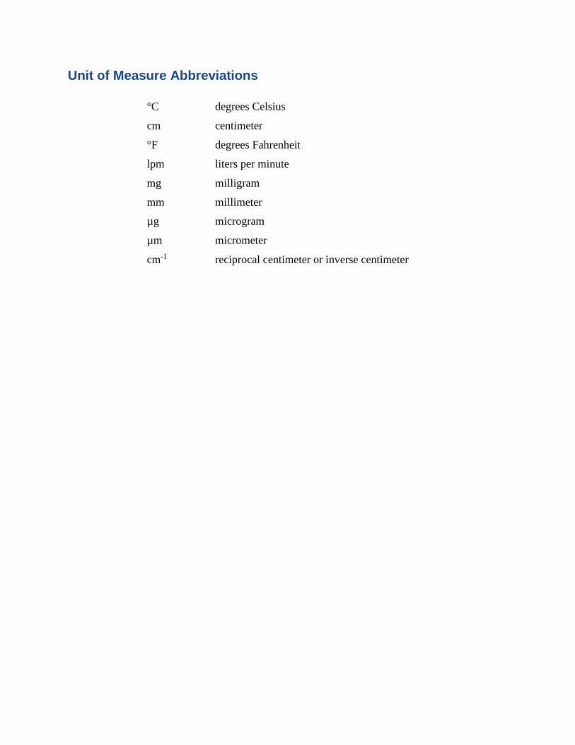
Unit of Measure Abbreviations
°C degrees Celsius
cm centimeter
°F degrees Fahrenheit
lpm liters per minute
mg milligram
mm millimeter
µg microgram
µm micrometer
cm-1 reciprocal centimeter or inverse centimeter
Definitions
Amorphous silica a non-crystalline form of silica which, if present, interferes
with the accurate quantification of crystalline forms,
including quartz
Apodization a mathematical process used in FTIR analysis to smooth
the signal
Background (spectrum) a measurement taken prior to sample measurement: if a
clean filter is used the spectral features of the filter media
are reduced, and environmental features such as water
vapor and carbon dioxide are largely eliminated (or
reduced) when the sample is analyzed
Baseline correction a mathematical adjustment to decrease a curvature or slope
in a sample spectrum; see Figure 6 for an illustration of the
effect of baseline correction; various correction algorithms
can be used
Commodity a product or group of products that is mined at a particular
operation; may also be considered a subsector within the
mining industry
Correction factor a mathematical adjustment made in the FAST software to
account for mineral content of respirable dust and other
factors that may otherwise decrease the accuracy of the
respirable crystalline silica quantification; uses standard
analysis results from an accredited laboratory as the
reference method
Cristobalite a form of crystalline silica, less commonly encountered
than quartz
Desiccant a material used to absorb excess moisture or humidity
Direct-on-filter analysis that can be completed on the aerosol sampling
filter on which the sample is collected, without altering the
sample filter or the collected sample
Field-based monitoring any exposure monitoring activity that can be completed
where the sample is collected at the work site, without the
need to send samples to an off-site laboratory for analysis
Focal point the point at which the rays of the infrared beam converge
and are most concentrated, and where the sample should be
positioned
Fourier transform infrared
spectroscopy
an analytical method capable of collecting a high resolution
infrared (absorption) spectrum for a sample over a broad
spectral range and converting the raw data in a spectrum
using Fourier transform
Integration the calculation of the area of a specific region of the sample
spectrum; the integrated value is correlated to the amount
of a substance that is present
Interference a species that interferes with the analysis of quartz, possibly
impacting the accuracy of the quantification of quartz
Limit of detection the lowest amount of a substance that is detected with
confidence by an analytical method; below this quantity,
the signal may be due to random noise rather than to the
presence of the substance
Limit of quantification the lowest amount of a substance that is quantifiable with
confidence by an analytical method; below this quantity,
the amount cannot be quantified with confidence, though
the substance can be identified with confidence if the limit
of detection (which is always less than the limit of
quantification) has been met
Macro a series of software instructions that can be executed as one
procedure; for field-based monitoring, the available macros
(from NIOSH) first execute a baseline correction of the
spectrum and then integrate the areas of interest; in some
software packages, the NIOSH macro may also export
sample results or generate a sample report
Non-destructive any method of analysis where the sample is not altered or
disturbed—that is, the sample is preserved in its original
form and remains available for analysis using other
analytical approaches
Quality Assurance (QA) sample a sample taken for quality assurance purposes that is
analyzed at the beginning of each session, with the results
compared to previous data to confirm that the instrument
hardware and software are generating consistent and
reliable results
Quartz (alpha quartz) the most common form of crystalline silica
Real-time monitoring a specific type of field-based monitoring in which results
are available after very short data collection periods (on the
order of seconds), enabling changes in conditions (e.g., dust
concentration) to be measured as they occur
Resolution the minimum difference in frequency that can be
distinguished within the spectrum; increasing the resolution
increases the level of detail that is visible
Respirable crystalline silica particles of crystalline silica small enough to reach the
alveolar region of the lungs when inhaled
Respirable dust particles of dust (of any composition) small enough to
reach the alveolar region of the lungs when inhaled
Sample bracket a NIOSH-designed component that is installed in the FTIR
instrument (replacing the original bracket of the
instrument) to accept the sample cradle or the sample
holder, ensuring the correct position of the sample for
analysis
Sample cradle or holder a NIOSH-designed component that is inserted in the sample
bracket to accept either the four-piece cassette (cradle) or
the dust sampling capsule (holder), ensuring the correct
position of the sample for analysis
Site-specific quantification an adjusted quantification of RCS concentration specific to
a particular location or operation, based on previous
comparison of the (unadjusted) quantification generated by
the FAST software and standard laboratory analysis of the
same samples
Spectrum (spectra) a plot of the sample data generated by the FTIR instrument
and software (i.e., infrared absorbance at each
wavenumber); spectrum can refer to the visual plot of the
data or to the collection of individual data points
Standard analysis the laboratory-based analysis method that would typically
be used or accepted for exposure compliance purposes in a
particular sector or subsector; for respirable crystalline
silica analysis in the United States, see the following
methods: MSHA P-2 [MSHA 2013a], MSHA P-7 [MSHA
2013b], NIOSH 7500 [NIOSH 2003], NIOSH 7603
[NIOSH 2017b], OSHA ID-142 [OSHA 2015]
Tridymite a form of crystalline silica, less commonly encountered
than quartz

Direct-on-filter Analysis for Respirable Crystalline Silica Using a Portable FTIR Instrument
Lauren G. Chubb and Emanuele G. Cauda
Introduction
Respirable crystalline silica (RCS) exposure occurs in many industries, and the potential health
effects of RCS have been well-documented [NIOSH 2002]. Monitoring is an essential part of
any RCS exposure control plan, but the timeliness of results from the lab and the cumulative cost
of analysis may limit the extent and the effectiveness of the monitoring process.
Field-based monitoring procedures offer a supplement to sample analysis completed by an offsite
laboratory. By eliminating the time spent transporting samples and waiting for laboratory results,
results are available the same day or the next day to allow operators to make decisions regarding
controls. This enhances the ability to collect data more effectively, enables better control over
potential exposures, and protects worker health.
This document details how to implement field-based monitoring for RCS. It is primarily intended
for industrial hygienists and other workers with health and safety responsibilities, specifically
within the mining industry (although workers in other industries may also find it useful). The
document has been written for a user with experience in respirable dust or RCS exposure
assessment but who does not necessarily have specialized training in analytical techniques. The
following topics are covered:
• General instructions for how to set up the equipment and the software required for field-
based RCS monitoring.
• Technical details of the monitoring method with explanations of why they are important.
• Quality assurance procedures to ensure consistent data.
• Examples and case studies on how to use different types of samplers in conjunction with
field-based monitoring.
• Links to additional resources for field-based monitoring (see Appendix A).
• Checklists to guide users through the process quickly (see Appendix B).
The NIOSH Manual of Analytical Methods contains sampling guidance for RCS in particular
[NIOSH 2003a] and for aerosols in general [NIOSH 2016b].
This document contains guidance applicable to portable Fourier transform infrared spectroscopy
(FTIR) instruments in general, though some instrument-specific guidance is also provided where
necessary. While researchers from the National Institute for Occupational Safety and Health
(NIOSH) have conducted extensive investigation on the use of four portable Fourier transform
infrared spectroscopy (FTIR) instruments [Ashley et al. 2020], other models of FTIR instruments
may also be available and compatible with field-based monitoring.
At the time this document was published, direct-on-filter analysis with portable FTIR was not a
stand-alone NIOSH analytical method or a standard analytical method used by MSHA or OSHA
2
or other international bodies. The role of field-based monitoring should be to act in support of
maintaining regulatory compliance by facilitating faster and more thorough assessment of RCS
levels. When there is a need for a formal assessment of compliance status, the dust samples
analyzed in the field should also be submitted to an accredited laboratory.
The field-based RCS monitoring approach presented here has been designed for respirable alpha
quartz, which is the most common crystalline silica polymorph. The analysis is not currently
optimized for other regulated crystalline silica polymorphs, cristobalite and tridymite, which can
both impact the accuracy of the field-based analysis if they are present. In most mining
environments, quartz is likely to be the only form of RCS present, but it is important to know if
either cristobalite or tridymite has been reported in respirable samples (based on previous
laboratory analyses). The term RCS will be used throughout this document except where more
specificity is required.
Technical Note
The approach to field-based monitoring described in this document and the quantification models
used in the NIOSH-developed Field Analysis of Silica Tool (FAST) software were developed
using 37-mm, 5-µm pore polyvinyl chloride (PVC) filters housed in 4-piece conductive cassettes
with stainless steel support (rather than a cellulose backing pad), or 37-mm, 5-µm pore polyvinyl
chloride (PVC) filters (within a capsule) housed in the dust sampling cassette with stainless steel
support (see Figure 2). The models were calibrated using crystalline silica (quartz) particles
(primarily Min-U-Sil 5, with NIST 1878a samples evaluated to confirm similarity) aerosolized in
laboratory dust chambers. Calibration samples were analyzed using a Bruker Optics Alpha
infrared spectrometer in transmission mode. Sixteen co-added sample scans were analyzed at a
resolution of 4 cm-1 using Blackman Harris 3-term apodization. Samples were subsequently
processed using a concave rubberband baseline correctiona (10 iterations) with 64 baseline
points.
a Though a complete definition is beyond the scope of this document, a “concave rubberband correction” is a
specific type of baseline correction that imagines a rubberband stretched between the two ends of the spectrum. The
correction is applied iteratively, with the number of iterations determining the intensity of the correction.
Other options for instrument analysis parameters are listed in Table 2. The spectral region
between 816 and 767 cm-1 was integrated, and calibrated models were developed from the
regression of the integrated area vs. gravimetric mass of crystalline silica (quartz).
When possible, field-based monitoring for crystalline silica is best completed using the same
filters, cassettes, and operational settings listed above. Field-based monitoring may still be
completed using different filter media, cassettes, and settings, but this may result in error or
uncertainty in crystalline silica quantification.
For additional information regarding the development of field-based, direct-on-filter analysis, see
Miller et al. [2012], Miller et al. [2013], Cauda et al. [2016], and Chubb and Cauda [2021]. This
document is representative of all relevant findings to date, but research is ongoing in this area
and additional findings will be published and made available to the public in the future.
3
Overview of Field-based Monitoring
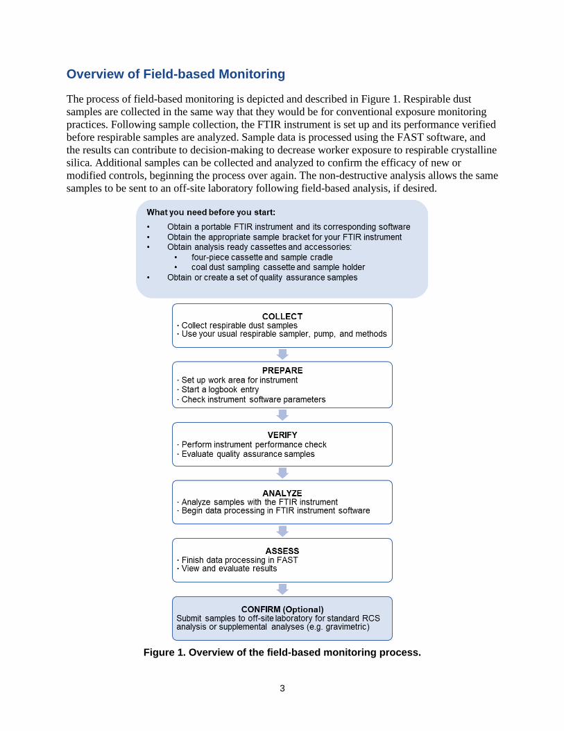
The process of field-based monitoring is depicted and described in Figure 1. Respirable dust
samples are collected in the same way that they would be for conventional exposure monitoring
practices. Following sample collection, the FTIR instrument is set up and its performance verified
before respirable samples are analyzed. Sample data is processed using the FAST software, and
the results can contribute to decision-making to decrease worker exposure to respirable crystalline
silica. Additional samples can be collected and analyzed to confirm the efficacy of new or
modified controls, beginning the process over again. The non-destructive analysis allows the same
samples to be sent to an off-site laboratory following field-based analysis, if desired.
Figure 1. Overview of the field-based monitoring process.
4
Field-based monitoring does not require laboratory experience or training but does require
careful execution to ensure reliable data; it should be part of a well-planned RCS exposure
assessment strategy and used in conjunction with routine laboratory analysis of respirable
samples. Previous experience in industrial hygiene or exposure assessment is recommended for
users of field-based monitoring. Although FTIR instruments are generally designed to be user-
friendly for non-expert users, NIOSH recommends contacting the manufacturer for assistance
with initial instrument setup and with basic instrument training.
Getting Started: Hardware and Software
Table 1 depicts and describes the hardware and software requirements. These requirements are in
addition to the personal sampling pumps and respirable cyclone samplers that are typically used.
The analysis of samples collected by impactor-type respirable samplers is not currently
supported by this field-based monitoring technique.
5
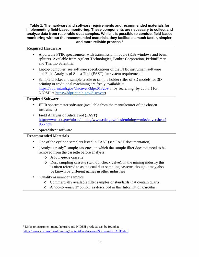
Table 1. The hardware and software requirements and recommended materials for implementing field-based monitoring. These components are necessary to collect and analyze data from respirable dust samples. While it is possible to conduct field-based monitoring without the recommended materials, they facilitate a much faster, simpler,
and more reliable process.b
b Links to instrument manufacturers and NIOSH products can be found at
https://www.cdc.gov/niosh/mining/content/HandwareandSoftwareforFAST.html.
Required Hardware
• A portable FTIR spectrometer with transmission module (KBr windows and beam
splitter). Available from Agilent Technologies, Bruker Corporation, PerkinElmer,
and Thermo Scientific
• Laptop computer; see software specifications of the FTIR instrument software
and Field Analysis of Silica Tool (FAST) for system requirements
• Sample bracket and sample cradle or sample holder (files of 3D models for 3D
printing or traditional machining are freely available at
https://3dprint.nih.gov/discover/3dpx013209 or by searching (by author) for
NIOSH at https://3dprint.nih.gov/discover)
Required Software
• FTIR spectrometer software (available from the manufacturer of the chosen
instrument)
• Field Analysis of Silica Tool (FAST)
http://www.cdc.gov/niosh/mining/www.cdc.gov/niosh/mining/works/coversheet2
056.htm
• Spreadsheet software
Recommended Materials
• One of the cyclone samplers listed in FAST (see FAST documentation)
• “Analysis-ready” sample cassettes, in which the sample filter does not need to be
removed from the cassette before analysis
o A four-piece cassette
o Dust sampling cassette (without check valve); in the mining industry this
is often referred to as the coal dust sampling cassette, though it may also
be known by different names in other industries
• “Quality assurance” samples
o Commercially available filter samples or standards that contain quartz
o A “do-it-yourself” option (as described in this Information Circular)
6
Conducting Field-based Analysis for Respirable Crystalline Silica
After respirable dust samples have been collected, RCS is quantified by FTIR analysis.
This section describes the analysis parameters that should be used to produce the most
reliable results and outlines procedures for verifying that the instrument and its settings are
appropriately configured before proceeding with sample analysis.
Setting Instrument Analysis Parameters
Research conducted at NIOSH has indicated that the following parameters for analysis with a
portable FTIR instrument provide the optimal balance necessary to obtain accurate and
reproducible data in a reasonable period of time. For example, higher resolutions result in more
data points per sample, and increased scan accumulations decrease noise (variation) in the data,
but both come at a cost of longer analysis times. Table 2 summarizes the relevant parameters and
settings used by NIOSH to develop the field-based method.
These parameters are important to the integrity of the data, and therefore it is essential to ensure
that the portable FTIR instrument is configured to these parameters before it is used for the
application described in this document. The top (unshaded) portion of the table contains basic
parameters that should be selected, regardless of the particular instrument or software used.
Modifying these settings will impact analysis results and may invalidate the results. The bottom
(shaded) portion of the table contains more advanced parameters, which may not be available for
some instruments or software programs. While it is advisable to match these parameters, if
available, they are less significant. Regardless, it is important that the same parameter options are
used consistently from sample to sample and day to day.
7
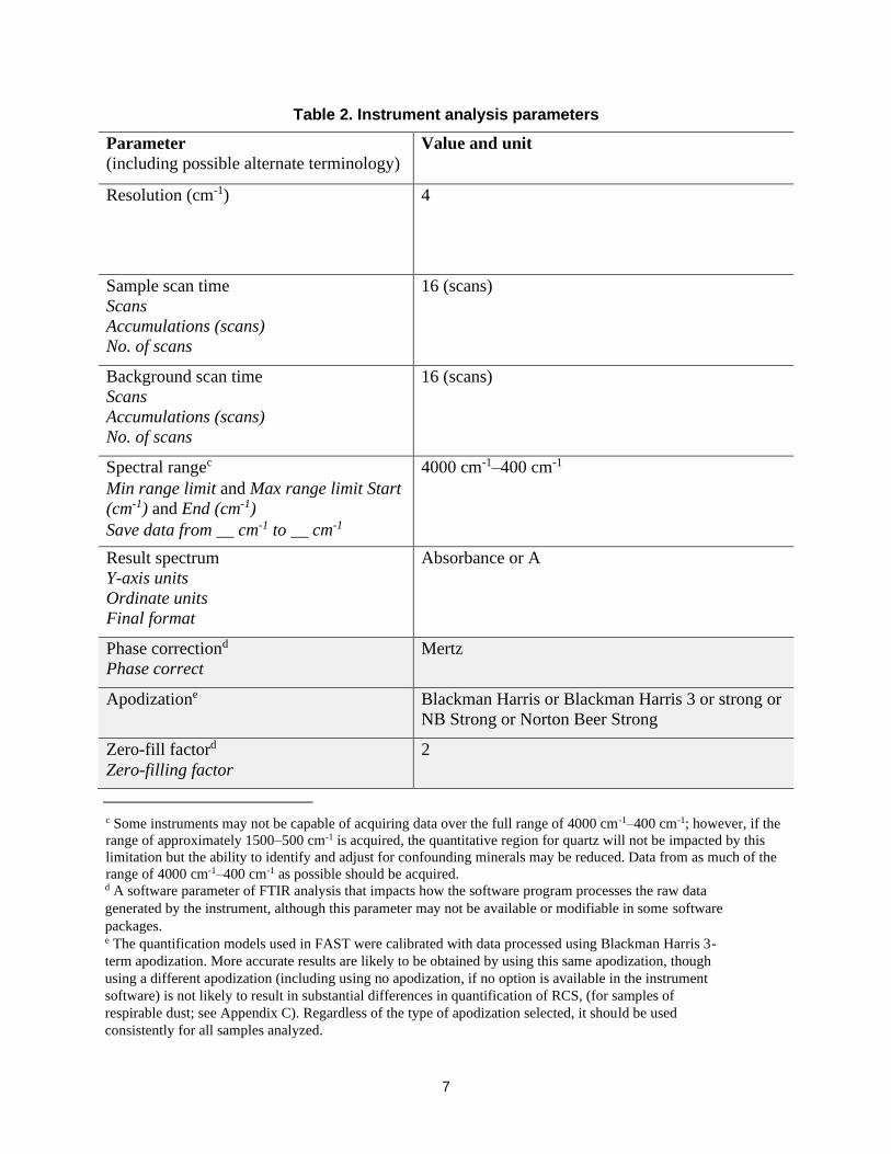
Table 2. Instrument analysis parameters
Parameter
(including possible alternate terminology)
Value and unit
Resolution (cm-1) 4
Sample scan time
Scans
Accumulations (scans)
No. of scans
16 (scans)
Background scan time
Scans
Accumulations (scans)
No. of scans
16 (scans)
Spectral rangec
Min range limit and Max range limit Start
(cm-1) and End (cm-1)
Save data from __ cm-1 to __ cm-1
4000 cm-1–400 cm-1
Result spectrum
Y-axis units
Ordinate units
Final format
Absorbance or A
Phase correctiond
Phase correct
Mertz
Apodizatione Blackman Harris or Blackman Harris 3 or strong or
NB Strong or Norton Beer Strong
Zero-fill factord
Zero-filling factor
2
c Some instruments may not be capable of acquiring data over the full range of 4000 cm-1–400 cm-1; however, if the
range of approximately 1500–500 cm-1 is acquired, the quantitative region for quartz will not be impacted by this
limitation but the ability to identify and adjust for confounding minerals may be reduced. Data from as much of the
range of 4000 cm-1–400 cm-1 as possible should be acquired. d A software parameter of FTIR analysis that impacts how the software program processes the raw data
generated by the instrument, although this parameter may not be available or modifiable in some software
packages. e The quantification models used in FAST were calibrated with data processed using Blackman Harris 3-
term apodization. More accurate results are likely to be obtained by using this same apodization, though
using a different apodization (including using no apodization, if no option is available in the instrument
software) is not likely to result in substantial differences in quantification of RCS, (for samples of
respirable dust; see Appendix C). Regardless of the type of apodization selected, it should be used
consistently for all samples analyzed.
8
Verifying Instrument Integrity
When the instrument is not working properly, data quality will be impacted and the acquired data
may be less accurate. In order for the FTIR instrument to produce generally reliable data, the
internal optical components of the instrument must be in alignment and functioning according to
specifications. It may not be possible to easily perform a visual check of these components; the
software associated with each portable instrument has the capability to conduct a series of tests
to evaluate the performance of the instrument. Depending on the instrument, these tests may be
termed Systems Checks or Instrument Checks, Instrument Verification, Performance
Qualification (PQ), or Operation Qualification (OQ). Regardless of terminology, the tests should
generally include a check of the instrument signal-to-noise ratio and a check of the frequency
and alignment.
While the instrument will function even if these tests are not performed, the acquired data may
not be accurate. It is recommended to perform these tests on a regular basis, such as weekly, and
in cases where the instrument may have been handled roughly (such as when shipped by a carrier
service, or as checked baggage with an airline), or has changed environments drastically (such as
from an arid climate to a humid climate or from a cold environment to a warm one). As the
instrument and its internal components age, some components will need to be replaced, and
regular performance testing can indicate when this is necessary.
When the performance tests are carried out routinely, they will indicate potential performance
concerns before data quality is affected; if performance tests are not carried out regularly, low-
quality data may go unnoticed. See the Quality Assurance (QA) Sample Spectra section for
additional information on verifying that the instrument is producing accurate and reproducible
data over time.
Inserting the Sample in the Instrument
Once the portable FTIR is set up with the proper analysis parameters and the integrity of the
instrument has been verified via performance tests, it is important to understand how to use the
portable instrument for the analysis of respirable dust samples using the modality generally
referred to as “direct-on-filter.” A few constraints and requirements need to be met to ensure that
accurate results are obtained using direct-on-filter analysis.
When using a four-piece cassette, the top (inlet) piece and bottom (outlet) piece of the cassette
should be removed from the two middle sections before being placed in the sample cradle. When
using the dust sampling cassette, the foil capsule should be carefully removed from the plastic
outer cassette before the capsule is placed in the sample holder.
The following pictures and directions (Figures 2–4) provide guidelines on how to position the
samples inside the portable FTIR. In general, it is good practice to position the sample with the
sample side facing the infrared source, which is typically on the left.
9
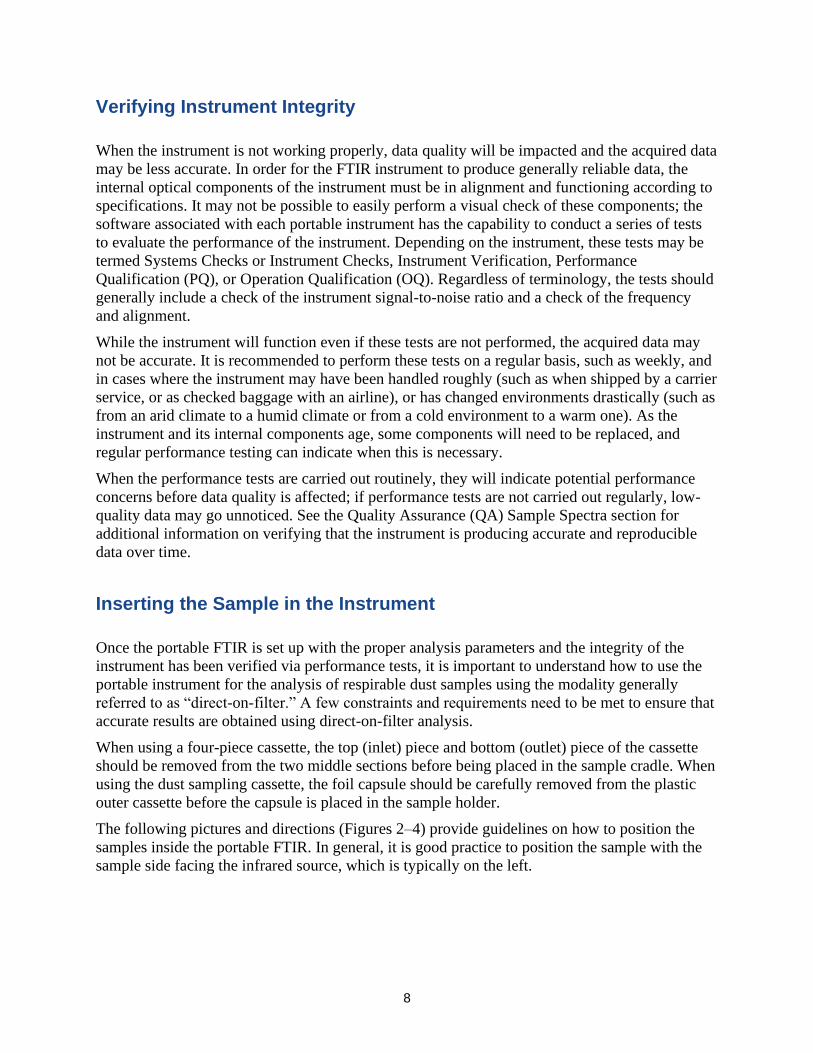
Figure 2. Examples of suitable sample cassettes (which allow the filter media to remain secured in the cassette or capsule) for field-based analysis. The holder or cassette
containing the filter media with the sample should be open on both sides, which can be accomplished by removing the top and bottom cassette pieces of the four-piece cassette (top) or removing the capsule from the dust sampling cassette (bottom). From one side
the dust material on the filter (or a portion of the filter, in the case of dust sampling capsule) should be visible, and from the other side the underside of the filter media
should be exposed and the support ring should be visible.
Photos by NIOSH
10
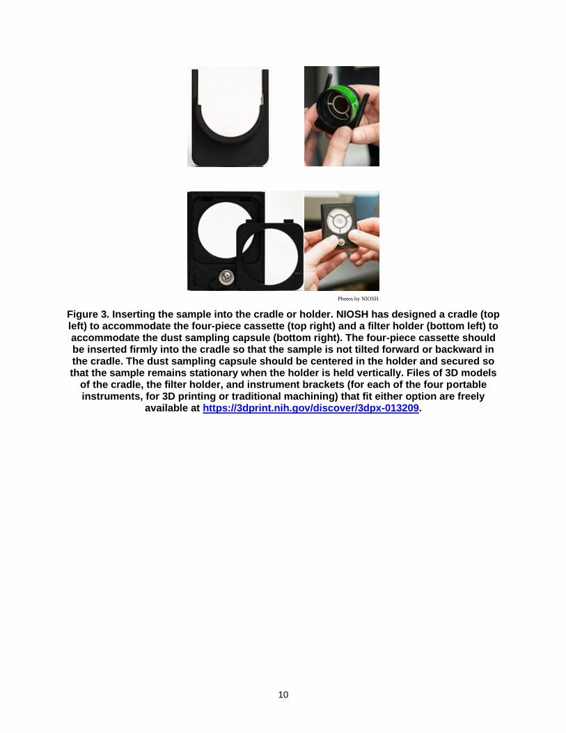
Figure 3. Inserting the sample into the cradle or holder. NIOSH has designed a cradle (top left) to accommodate the four-piece cassette (top right) and a filter holder (bottom left) to accommodate the dust sampling capsule (bottom right). The four-piece cassette should be inserted firmly into the cradle so that the sample is not tilted forward or backward in the cradle. The dust sampling capsule should be centered in the holder and secured so that the sample remains stationary when the holder is held vertically. Files of 3D models
of the cradle, the filter holder, and instrument brackets (for each of the four portable instruments, for 3D printing or traditional machining) that fit either option are freely
available at https://3dprint.nih.gov/discover/3dpx-013209.
Photos by NIOSH
11
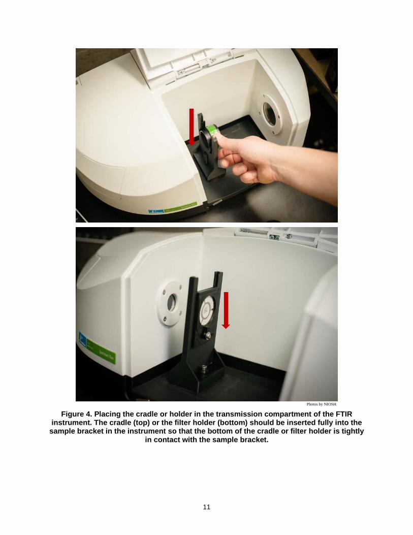
Figure 4. Placing the cradle or holder in the transmission compartment of the FTIR instrument. The cradle (top) or the filter holder (bottom) should be inserted fully into the
sample bracket in the instrument so that the bottom of the cradle or filter holder is tightly in contact with the sample bracket.
Photos by NIOSH
12
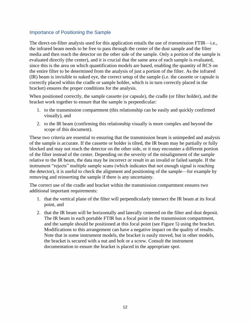
Importance of Positioning the Sample
The direct-on-filter analysis used for this application entails the use of transmission FTIR—i.e.,
the infrared beam needs to be free to pass through the center of the dust sample and the filter
media and then reach the detector on the other side of the sample. Only a portion of the sample is
evaluated directly (the center), and it is crucial that the same area of each sample is evaluated,
since this is the area on which quantification models are based, enabling the quantity of RCS on
the entire filter to be determined from the analysis of just a portion of the filter. As the infrared
(IR) beam is invisible to naked eye, the correct setup of the sample (i.e. the cassette or capsule is
correctly placed within the cradle or sample holder, which is in turn correctly placed in the
bracket) ensures the proper conditions for the analysis.
When positioned correctly, the sample cassette (or capsule), the cradle (or filter holder), and the
bracket work together to ensure that the sample is perpendicular:
1. to the transmission compartment (this relationship can be easily and quickly confirmed
visually), and
2. to the IR beam (confirming this relationship visually is more complex and beyond the
scope of this document).
These two criteria are essential to ensuring that the transmission beam is unimpeded and analysis
of the sample is accurate. If the cassette or holder is tilted, the IR beam may be partially or fully
blocked and may not reach the detector on the other side, or it may encounter a different portion
of the filter instead of the center. Depending on the severity of the misalignment of the sample
relative to the IR beam, the data may be incorrect or result in an invalid or failed sample. If the
instrument “rejects” multiple sample scans (which indicates that not enough signal is reaching
the detector), it is useful to check the alignment and positioning of the sample—for example by
removing and reinserting the sample if there is any uncertainty.
The correct use of the cradle and bracket within the transmission compartment ensures two
additional important requirements:
1. that the vertical plane of the filter will perpendicularly intersect the IR beam at its focal
point, and
2. that the IR beam will be horizontally and laterally centered on the filter and dust deposit.
The IR beam in each portable FTIR has a focal point in the transmission compartment,
and the sample should be positioned at this focal point (see Figure 5) using the bracket.
Modifications to this arrangement can have a negative impact on the quality of results.
Note that in some instrument models, the bracket is easily moved, but in other models,
the bracket is secured with a nut and bolt or a screw. Consult the instrument
documentation to ensure the bracket is placed in the appropriate spot.
13
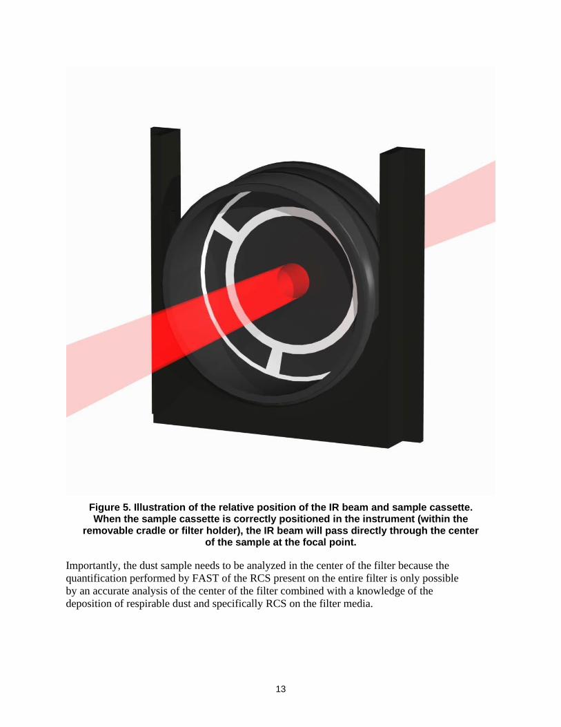
Figure 5. Illustration of the relative position of the IR beam and sample cassette. When the sample cassette is correctly positioned in the instrument (within the
removable cradle or filter holder), the IR beam will pass directly through the center of the sample at the focal point.
Importantly, the dust sample needs to be analyzed in the center of the filter because the
quantification performed by FAST of the RCS present on the entire filter is only possible
by an accurate analysis of the center of the filter combined with a knowledge of the
deposition of respirable dust and specifically RCS on the filter media.
14
NIOSH-developed Accessories for FTIR Instrumentation
At the focal point, the infrared beam in the four portable FTIR instruments evaluated by NIOSH
is fixed and ranges from 6 to 9 mm [Ashley et al. 2020], each of which is larger than the inlet
openings commonly found in the traditional three-piece sampling cassette. The material of the
cassette absorbs much of the IR beam, leaving insufficient signal for an accurate analysis.
Additionally, the IR beam cannot penetrate the cellulose backing pad typically used to support
the polyvinyl chloride (PVC) filter in the cassette, inhibiting the analysis of the sample. To
address these issues, the PVC filter can be removed from the cassette with tweezers and inserted
in a flat holder; however, this procedure requires additional handling which may induce sample
losses. For these reasons, adjustments are needed to the cassette that is used to collect the
respirable dust sample prior to the analysis, as described below.
NIOSH has designed specific cradles and brackets as accessories for a variety of holders,
cassettes, and different FTIR units. Files of 3D models for 3D printing or traditional machining
are freely available at https://3dprint.nih.gov/discover/3dpx-013209. These designs ensure the
correct positioning of the sample inside a portable FTIR unit. These designs are not the only
configurations possible, and other options can be created as long as the constraints described in
the above section (that is, the correct vertical and horizontal positioning of the sample filter in
the transmission compartment) are met.
Considerations for three types of samplers/cassettes are outlined below. Additional approaches
may be explored in the future for available samplers and their related holders/cassettes.
Four-piece Cassette
In order to minimize sample handling by keeping the filter in the cassette, NIOSH designed a
four-piece cassette with top and bottom portions that can be removed to expose the filter to the
IR beam while still containing the filter between two pieces of the cassette, and using a different
support design to allow transmission FTIR analysis. The resulting cassette (see Figure 2) is
compatible with a number of respirable samplers commonly used by industrial hygienists, many
of which are named in the NIOSH 0600 [NIOSH 1998], NIOSH 7500 [NIOSH 2003b], NIOSH
7602 [NIOSH 2017a], NIOSH 7603 [NIOSH 2017b], and OSHA ID-142 [OSHA 2015] methods
for respirable dust and RCS. The cassette was designed in collaboration with Zefon International
via a Cooperative Research and Development Agreement (CRADA). The product that resulted
from the collaboration is commercially available from Zefon International.
Dust Sampling Cassette
The sampling cassette used in coal mines as part of the coal mine dust personal sampler unit uses
a slightly different process than the four-piece cassette. The aluminum capsule that encloses the
filter media and the aluminum ring that supports the filter media allow transmission of enough of
the infrared beam to permit a reliable analysis of the sample. The capsule simply needs to be
removed from the plastic cassette and inserted in a filter holder (illustrated in the photo on the
bottom of Figure 3). Note that this sampling cassette is also available for compliance sampling
and includes a check valve, but this version of the cassette is not compatible with direct-on-filter
analysis.
15
While it is possible to use this sampling cassette for field-based monitoring, it is important to
consider that the cassette was not designed for this use specifically, and other cassette options
will likely provide more accurate results. This topic is discussed in Pampena et al. [2019].
Because of the potential for less accurate results, this type of cassette is most appropriate for
relative determinations of RCS (e.g., higher-exposure potential areas or tasks vs. lower-exposure
potential areas or tasks).
Other Sampling Cassette Types
The four-piece cassette described above was designed specifically for use with field-based
monitoring and is the preferred type of cassette for field-based monitoring. At the time this
document was published, only calibration models for the four-piece cassette and dust sampling
cassette (and respirable samplers that use these cassettes) were available in FAST. This section
briefly describes other cassettes and samplers that are physically compatible with field-based
analysis directly on the sample filter, but would require additional calibration models to be added
to FAST to facilitate their use with field-based monitoring.
• A new respirable sampler has been designed and tested by NIOSH [Lee et al. 2017]. The
sampler operates at 1.1 lpm and uses an innovative internal cassette with 25-mm PVC
filter media. The cassette has been designed to allow direct-on-filter analysis of the dust
sample with a portable FTIR. The performance of the sampler for respirable dust has
been validated. The prototype sampler can be produced via 3D printing using the
“Respirable size-selective sampler for end-of-shift quartz measurement” files available at
https://3dprint.nih.gov/discover/3dpx011762.
• There is also an interest in direct-on-filter analysis of dust samples collected by real-time
respirable dust monitors. The current analytical technologies used in real-time respirable
dust monitors cannot distinguish RCS within respirable dust. Some units collect a dust
sample on a filter after the dust sensor in order to protect the pump. The potential use of
these collected samples is being explored by NIOSH. With the use of the proper filter
media, the analysis of RCS is already possible (though RCS results are not available in
real-time). NIOSH is continuing to explore ways to facilitate this additional
implementation. Any change in the filter holder will need to be tested to confirm that the
performance of the monitor (with respect to respirable dust) is not adversely impacted.
• Respirable dust samples can be collected with other cassettes that could be suitable to
direct-on-filter analysis. The use of the Safety in Mines Personal Dust Sampler
(SIMPEDS) [Harris and Maguire 1968; Stacey et al. 2014; Stacey et al. 2013] is common
in countries outside the United States. Although this type of sampler is not currently
recommended for field-based monitoring, the cassette may be compatible with direct-on-
filter analysis, and the SIMPEDS sampler may be an option for field-based monitoring in
the future.
16
Generating Spectra
Background Spectrum
Before any sample can be scanned or analyzed, every portable FTIR instrument requires analysis
of a background spectrum. The FTIR analysis of a sample is a relative measurement—i.e., the
interaction of the IR beam with a sample compared to the interaction of the IR beam with a
reference. The background spectrum provides this reference. The general process used to
generate a background spectrum is similar for each instrument, although each instrument and
respective software has specific procedures. Consult the instrument software documentation (or
Help file) for more information.
For the application described in this document, the sample consists of respirable dust on a filter,
and the background spectrum is a clean filter (containing no respirable dust) of the same type. By
using a clean filter for the background spectrum, the contribution of the filter media to the
subsequent analysis of a sample (on similar filter media) will be minimized, resulting in a sample
spectrum that is a function primarily of the respirable dust. This can be accomplished by one of
two methods: analyzing a spectrum (with an empty transmission compartment used as the
background spectrum) for each filter before any dust is collected and subtracting that from the
sample spectrum later, or using a designated clean filter as the background spectrum for an entire
set of filters. Both methods will ultimately produce results of approximately the same quality
(see Appendix C). The designated clean filter method is preferred since it is much less
cumbersome and much more efficient for the user, although normal differences in filter thickness
mean that subtraction will reduce but not always eliminate the contribution of the filter.
If the clean filter method is used for the background spectrum, the following considerations
apply:
• The clean filter should be the same type of media used for the collection of the respirable
dust samples. In the United States, this is generally a 37-mm, 5-µm pore size PVC filter,
as indicated in the NIOSH methods 0600, 7500, 7602, 7603 [NIOSH 1998, 2003b,
2017a, 2017b].
• The clean filter used for the background spectrum can be selected from the blank filters
in the set of cassettes used for sampling and should be from the same manufacturer lot or
batch as the filters used for sampling. A good practice is to set aside a number of blanks
equivalent to 10% of the sampling set. An additional sample can be set aside as a clean
filter for the background spectrum. For example, if a health and safety professional is
planning to collect 20 respirable dust samples one day, two cassettes should be set aside
as blanks; an additional sample should be set aside as a clean filter to be used for the
background spectrum. (20 samples+2 blanks+1 clean filter for the background spectrum).
• The subtraction procedure described below is not required when a clean filter is used for
the background spectrum.
If the subtraction method is used, the following general procedure should be used:
1. Prior to sample collection, all filters to be used for sampling should be analyzed with the
portable FTIR instrument, using an empty transmission compartment for the background
spectrum. Data should be saved with filenames that correspond to the sample ID and
17
indicate that the spectrum represents a clean filter, before sample collection (e.g.
sample1_clean).
2. Following sample collection, all filters should be analyzed with the portable FTIR
instrument, using the empty transmission compartment for the background spectrum.
Data should be saved with filenames that correspond to the sample ID and indicate that
the spectrum represents a sample filter that now contains respirable dust (e.g.
sample1_dust).
3. Using the instrument software, subtract the “clean filter” spectrum for the “sample filter”
spectrum for each sample ID. Consult the software documentation for guidance on how
to use the software to subtract spectra. Be sure to save the new spectrum files resulting
from the subtraction procedure. It is recommended that the filename indicates that the
spectrum is the result of subtraction (e.g. sample1_subtracted).
4. All data processing to calculate RCS should use the subtracted spectrum files. The
“sample filter” spectrum using an empty transmission compartment for the background
measurement will not provide a reliable quantification of RCS.
Regardless of which approach to the background spectrum is taken, it is crucial that the filter
used as a background is clean (i.e., does not contain any dust and has not been touched) and is as
similar to the sample filters as possible. For instance, a filter that is perceptibly thicker or thinner
than other filters should not be used as the background because this could impact the quality of
sample results, especially for small quantities of RCS.
Quality Assurance (QA) Sample Spectra
It is important to ensure that the instrument performance remains consistent over time. One
element of regular performance checks should be the analysis of a set of four to seven quality
assurance, or QA, samples, which remain with the instrument and are each analyzed every time
the instrument is used. The calculated value of RCS should remain consistent over time for the
set of QA samples, indicating that the instrument performance is accurate; however, note that
these samples are not used to calibrate the instrument, as this is generally not necessary. See
Creating a Set of Samples to be Used as Quality Assurance Samples for guidance on establishing
a set of QA samples.
To track the QA sample results over time, the QA Sample Tracking spreadsheet (see Appendix A
for a complete list of resources for field-based monitoring) should be used together with this
document. The spreadsheet can accommodate up to ten QA samples. If multiple sets of QA
samples will be used (for example, for multiple instruments), it is recommended that a unique
spreadsheet is used for each set of QA samples.
To use the spreadsheet, the column headers in the “Input QA Sample Data” tab should be named
according to the sample IDs of the QA samples. Each time the QA samples are analyzed, the
results should be entered. The data should be typed directly into each cell rather than copied and
pasted, as this can interrupt some of the formatting that makes the spreadsheet function. The
spreadsheet calculates basic summary statistics for the data over time; this allows the spreadsheet
to flag any data point that is a statistical outlier. Approximately 10–20 data points are needed
before this function becomes a reliable indicator of true outliers; when there are only a few data
points, the spreadsheet may flag a data point that is only slightly different from the others. This
18
process can be accelerated by analyzing QA samples several times per day (e.g., in the morning
and again in the afternoon) for the first several days.
Each time the instrument is used (or daily, when the instrument is used multiple times throughout
the day), the QA samples should be analyzed and the data entered into the spreadsheet. Any of
the QA samples that are outliers will be highlighted automatically in the spreadsheet (unless
there are still too few data points for a reliable indication). The incidence of one outlier (while all
other QA samples are within normal variation) indicates that the problem is likely unique to that
particular sample and is therefore not likely to be indicative of a problem with the instrument
itself. Often this is a matter of a simple error during the analysis—e.g., the QA sample was not
inserted properly in the cradle (or filter holder) or the cradle was not properly inserted in the
bracket, the wrong QA sample was analyzed (or the spectrum was labeled incorrectly), or the
result was incorrectly entered in the spreadsheet (e.g. transposition of digits). It is also possible
that the QA sample was physically damaged prior to analysis, changing the result. Note that over
time, some QA samples may begin to lose material due to repeated use; QA samples should be
discarded when there is evidence of lost material. When one QA sample is an outlier, the
recommended action is to re-analyze the QA sample. If the result is within the normal range for
that sample (as indicated by previously saved results in the QA Sampling Tracking Spreadsheet),
then sample analysis should proceed as usual. If the result is still outside of the normal range, the
QA sample was likely damaged and should be discarded. The spreadsheet should be updated
accordingly and then sample analysis can proceed as usual.
The incidence of multiple outliers indicates a potential problem with the instrument. This could
be due to either hardware or software changes. It is important not to ignore irregular QA sample
data, because the problem will likely also impact the accuracy of subsequent sample data.
Irregularities should be noted in a logbook. A number of issues may occur that result in irregular
sample data, and a number of steps may help to identify the cause of the issues, including:
• Check that all data points are entered correctly, that samples have been labeled correctly,
and that no values have been transposed.
• Make sure that the background was properly scanned; this will typically require scanning
the clean filter again to produce a new background, paying particular attention to the
positioning of the clean filter in the transmission compartment. QA samples should be
reanalyzed after scanning the new background.
• Check the software analysis parameters to ensure that all parameters are correct (see the
Setting Instrument Analysis Parameters section).
• Complete the applicable performance verification/diagnostic tests to identify components
that may be beyond their service life or otherwise need to be replaced.
• Examine the instrument to observe any physical abnormalities that may be present (i.e.,
cracked, cloudy, or smudged windows and mirrors); if faulty components are identified,
replace them if possible. If faulty components are identified but cannot be immediately
replaced, contact the manufacturer for service recommendations.
• Replace the internal desiccant if there is reason to believe that humidity could be a factor
(note that the desiccant is not a user-serviceable part on all instrument types). While
excess humidity can affect the sample spectrum, it is mainly a concern due to the
19
potential for condensation on internal instrument components, which the desiccant
mitigates.
• Feel the outer casing of the instrument and note if it is warmer than usual. If the
instrument seems particularly warm, turn the instrument off and allow it to come to room
temperature before turning it on again.
If the source of the problem cannot be identified and resolved using the steps above, it may be
necessary to communicate directly with the manufacturer of the instrument for more advanced
diagnostic tools or to return the instrument to the manufacturer for service.
Sample Spectra
After the background spectrum has been generated and the instrument performance has been
verified by the QA sample analysis, sample spectra may be analyzed. Sample spectra should be
given unique identifiers that can be easily linked back to the identifiers on the physical samples.
The following section describes how sample data are processed and then interpreted to provide
meaningful results.
Processing Sample Data
After the spectrum of a sample is generated, the spectrum must also be processed by two
procedures: (1) a baseline correction, and (2) integration of areas of interest for crystalline silica
(quartz) and other minerals that might have a confounding effect in the quantification of RCS in
the sample. NIOSH has designed macros for the four FTIR instruments evaluated to facilitate the
processing of the analyzed samples. Each macro serves as a combination procedure that performs
the baseline correction, integrates the portions of the spectrum used for identification and
quantification, and reports values for these ranges of the spectrum. These macros are available
for users to download (https://github.com/niosh-mining/fast/) and import into their version of the
software, and they will be updated as areas are added and/or modified based on ongoing
research. To properly load macro and template files, see the FTIR software documentation.
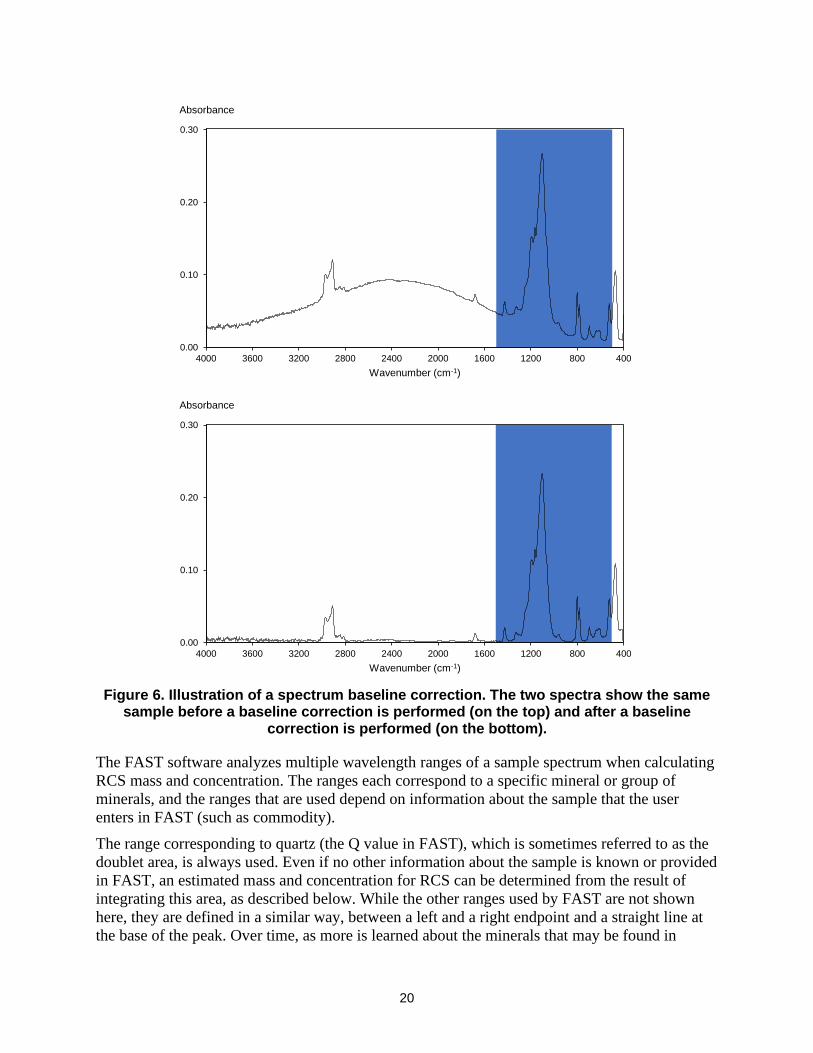
The baseline correction adjusts the spectrum to remove distortions such as slope or curvature in
the spectrum, as shown in Figure 6. While is it important to perform a baseline correction in
general, different software programs perform the correction differently. In some programs, only
a generic “baseline correction” option may be available. In other cases, there may be multiple
baseline correction options, often including an “auto baseline correction”. The most important
practice is to use the same option consistently for both QA samples and other samples; see
Appendix C for a comparison of several common options. In general, baseline correction
procedures can typically be accessed through the manipulate or transform menu; search or use
the Help file for the FTIR software if needed. Baseline correction should be performed over the
full range of the spectrum (e.g. 4000–400 cm-1). The NIOSH macros for the Bruker, Perkin
Elmer, and Thermo instruments include a baseline correction; spectra collected using the Agilent
software should be baseline corrected manually.
20
Figure 6. Illustration of a spectrum baseline correction. The two spectra show the same sample before a baseline correction is performed (on the top) and after a baseline
correction is performed (on the bottom).
0.00
0.10
0.20
0.30
40080012001600200024002800320036004000
Absorbance
Wavenumber (cm-1)
0.00
0.10
0.20
0.30
40080012001600200024002800320036004000
Absorbance
Wavenumber (cm-1)
The FAST software analyzes multiple wavelength ranges of a sample spectrum when calculating
RCS mass and concentration. The ranges each correspond to a specific mineral or group of
minerals, and the ranges that are used depend on information about the sample that the user
enters in FAST (such as commodity).
The range corresponding to quartz (the Q value in FAST), which is sometimes referred to as the
doublet area, is always used. Even if no other information about the sample is known or provided
in FAST, an estimated mass and concentration for RCS can be determined from the result of
integrating this area, as described below. While the other ranges used by FAST are not shown
here, they are defined in a similar way, between a left and a right endpoint and a straight line at
the base of the peak. Over time, as more is learned about the minerals that may be found in
21
respirable dust and how they might impact the accuracy of field-based RCS quantification, more
ranges for analysis may be added to FAST, or the existing ranges may be modified to improve
overall accuracy.
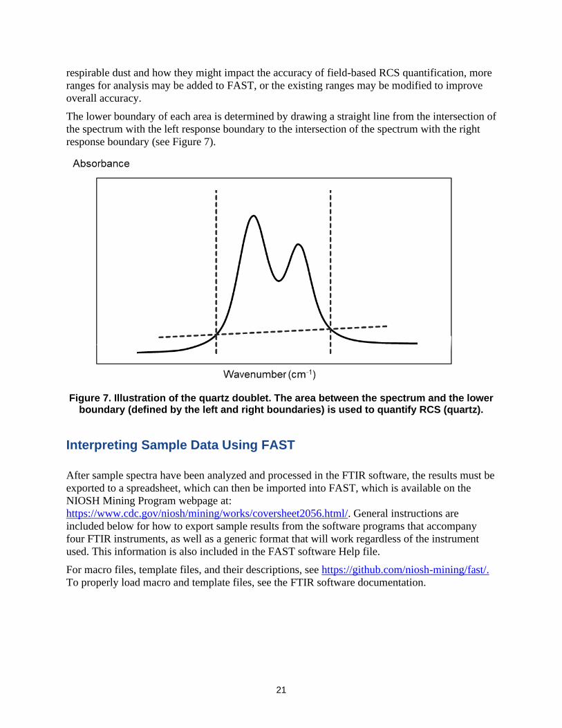
The lower boundary of each area is determined by drawing a straight line from the intersection of
the spectrum with the left response boundary to the intersection of the spectrum with the right
response boundary (see Figure 7).
Figure 7. Illustration of the quartz doublet. The area between the spectrum and the lower boundary (defined by the left and right boundaries) is used to quantify RCS (quartz).
Interpreting Sample Data Using FAST
After sample spectra have been analyzed and processed in the FTIR software, the results must be
exported to a spreadsheet, which can then be imported into FAST, which is available on the
NIOSH Mining Program webpage at:
https://www.cdc.gov/niosh/mining/works/coversheet2056.html/. General instructions are
included below for how to export sample results from the software programs that accompany
four FTIR instruments, as well as a generic format that will work regardless of the instrument
used. This information is also included in the FAST software Help file.
For macro files, template files, and their descriptions, see https://github.com/niosh-mining/fast/.
To properly load macro and template files, see the FTIR software documentation.
22
Exporting Results from Agilent
In RESOLUTIONS PRO
1. Open a new Multi-Spectral Document by selecting File >> New >> Multi-Spectral
Document >> OK
2. Open all spectra files to be included in the report by selecting Open >> (select files) >>
Open
3. Add each sample spectrum into the Multi-Spectral Document by dragging or copying the
file:
a. To drag:
i. Click the + next to the sample name to expand.
ii. Click on the spectrum entry and drag it to the Multi-Spectral Document.
iii. Check the Multi-Spectral Document to confirm that the sample file was
successfully transferred or copied.
b. To copy:
i. Click the + next to the sample name to expand.
ii. In the data grid in the lower portion of the screen, highlight Row 1. iii. Right-click and select Copy (or use Ctrl+C). iv. Click on the + next to the
Multi-Spectral Document to expand.
iii. In the data grid in the lower portion of the screen, place the cursor in the
first empty row.
iv. Right-click and select Paste (or use Ctrl+V).
4. When all samples have been added to the Multi-Spectral Document, use the Ctrl key to
highlight each row of the grid.
5. Select Analysis >> Peak Options >> New Peak Template (all spectra).
6. In the Creation Choices field (top), select Create a set from file.
7. Select Browse and choose the Peak-area.def file. Select Open >> OK.
8. Use the Ctrl key to select the columns for Name, K, Q, C, D, and M.
9. Right-click and select Copy (or use Ctrl+C).
In EXCEL
1. Place the cursor in cell A1; right-click and select Paste (or use Ctrl+V).
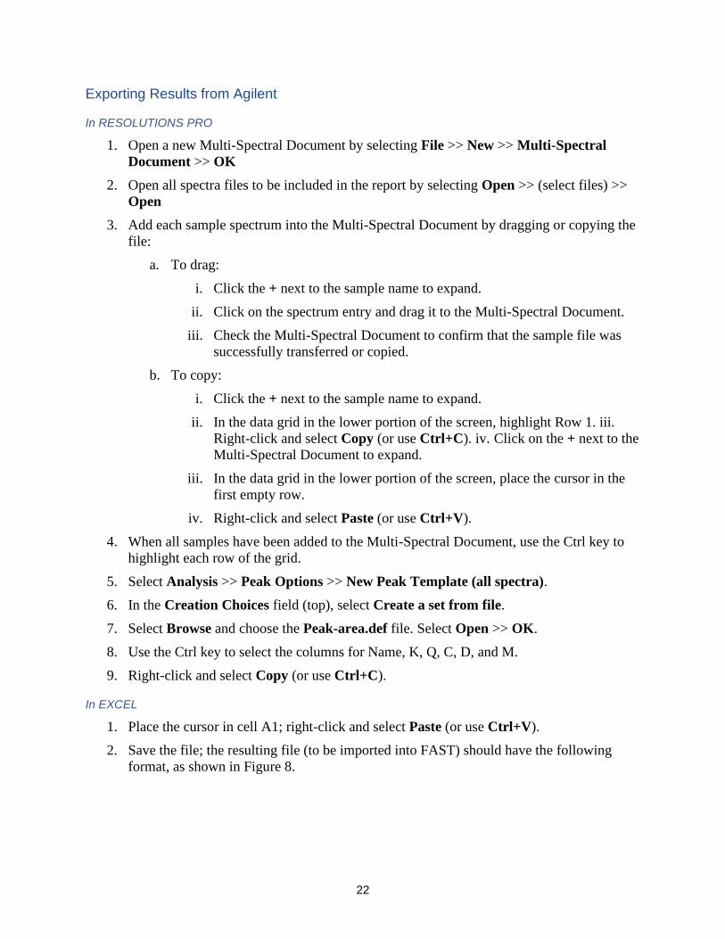
2. Save the file; the resulting file (to be imported into FAST) should have the following
format, as shown in Figure 8.
23
Figure 8. Results format from the Resolutions Pro software (Agilent). The results report exported from Resolutions Pro displays data for each sample in a row format. The Sample ID should appear in Column A, followed by the result areas beginning in
Column B.
A B C D E F
1 Name K Q C D M
2 sample1_0000(1) 0.034 0.704 -0.043 -0.036 -0.03
3 sample2_0000(1) 0.019 0.145 -0.006 -0.006 -0.02
4 sample3_0000(1) 0.015 1.722 -0.015 -0.012 -0.017
Exporting Results from Bruker
In OPUS
1. Select Print >> Generate Report.
2. On the Select Files tab of the menu that appears, select Multi sample report, and load
the template file silica_report.art.
3. Select Load and navigate to the Processed_Spectra folder (or the location where
processed files have been saved), then select the sample files to be included in the report.
4. Select the Output to tab; on the menu that appears, check that the csv file option is
selected, then specify a name for the report file.
5. Specify a file path for the saved report, then select Generate.
In EXCEL
1. Open the saved report spreadsheet and highlight Column A.
2. Select the Data >> Text to Columns.
3. Select Delimited and click Next; select Semicolon and click Finish.
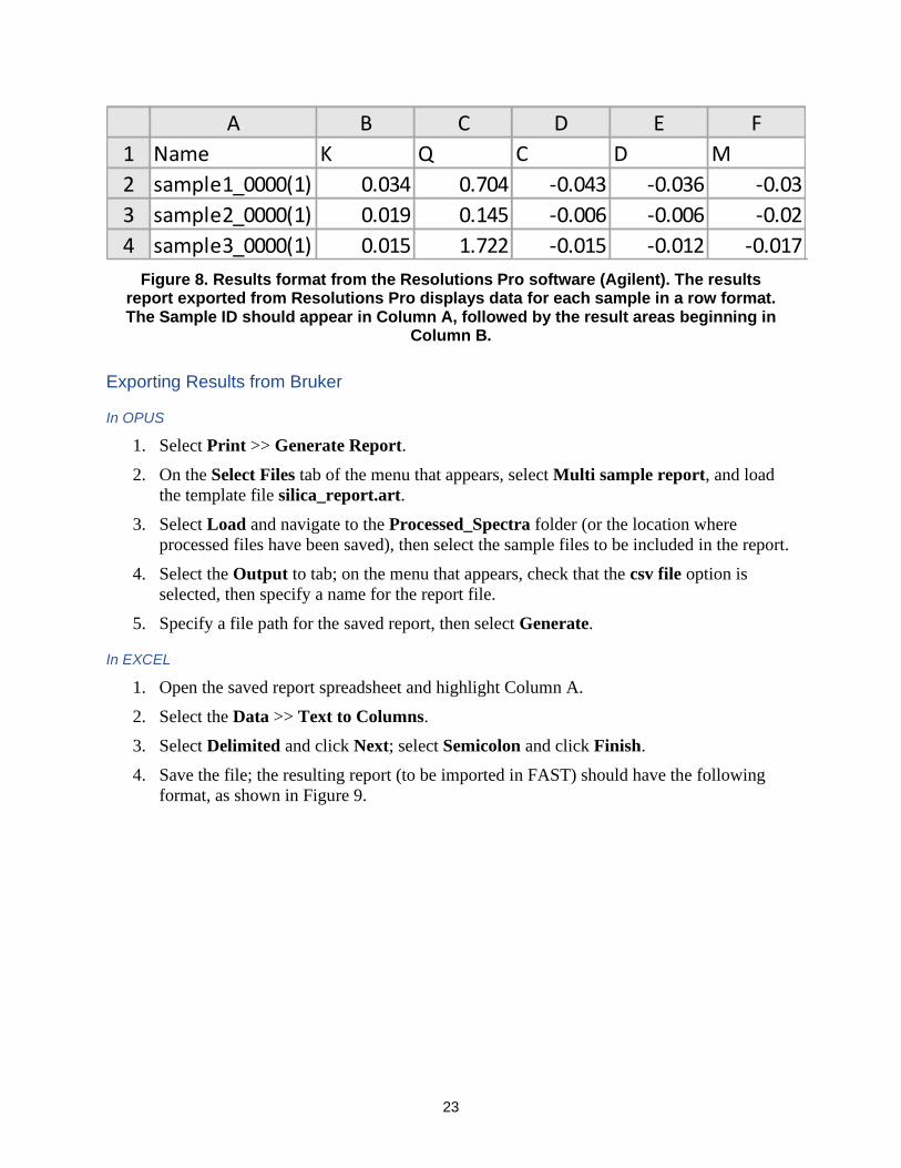
4. Save the file; the resulting report (to be imported in FAST) should have the following
format, as shown in Figure 9.
24
Figure 9. Results format from the Opus software (Bruker). The results report exported from Opus displays data for each sample in a column format rather than a row format. Column B must contain the sample ID, and column C must contain the result areas for
samples.
A B C D E
1 No Spectrum file nameResult Freq.1 Freq.2
2 1 sample1 0.704 816 767
3 0.034 930 900
4 -0.03 740 720
5 -0.036 743 718
6 -0.043 890 865
7 2 sample2 0.145 816 767
8 0.019 930 900
9 -0.02 740 720
10 -0.006 743 718
11 -0.006 890 865
12 3 sample3 1.722 816 767
13 0.015 930 900
14 -0.017 740 720
15 -0.012 743 718
16 -0.015 890 865
Exporting Results from Perkin Elmer
In SPECTRUM 10
1. Open all samples files to be included in the report.
2. Select Process >> Macro >>Silica est.
3. With the Results Table open, select File >> Send To >> Excel.
In EXCEL
1. To simplify the spreadsheet, keep the Sample Name, Q, K, M, D, and C columns
(Columns A, E, F, G, H, I) for the processed files; all other cells can be deleted.
25
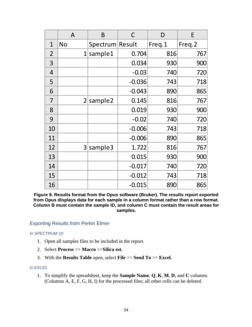
2. Save the file; the resulting report (to be imported in FAST) should have the following
format, as shown in Figure 10.
Figure 10. Results format from the Spectrum software (PerkinElmer). The results report exported from Spectrum displays data for each sample in a row format. The Sample ID
should appear in Column A, followed by the result areas beginning in Column B.
A B C D E F
1 Sample Name q k m d c
2 sample1.SPA_2 0.704 0.034 -0.03 -0.036 -0.043
3 sample2.SPA_2 0.145 0.019 -0.02 -0.006 -0.006
4 sample3.SPA_2 1.722 0.015 -0.017 -0.012 -0.015
Exporting Results from Thermo Fisher
In TQ ANALYST EZ EDITION
1. Open the TQ Analyst EZ Edition program.
2. From the File menu, select Open Method…, then select the Silica_int.qnt method and
click Open.
3. From the Diagnostics menu, select Multiple Summary – Select Files… Select the
sample files to be included in the report. TQ Analyst EZ Edition will generate and open a
spreadsheet containing the results.
In EXCEL
1. Depending on the version/settings of TQ Analyst EZ Edition, the format of the results
spreadsheet may differ slightly; delete columns as needed so that the format of the
spreadsheet is as shown below.
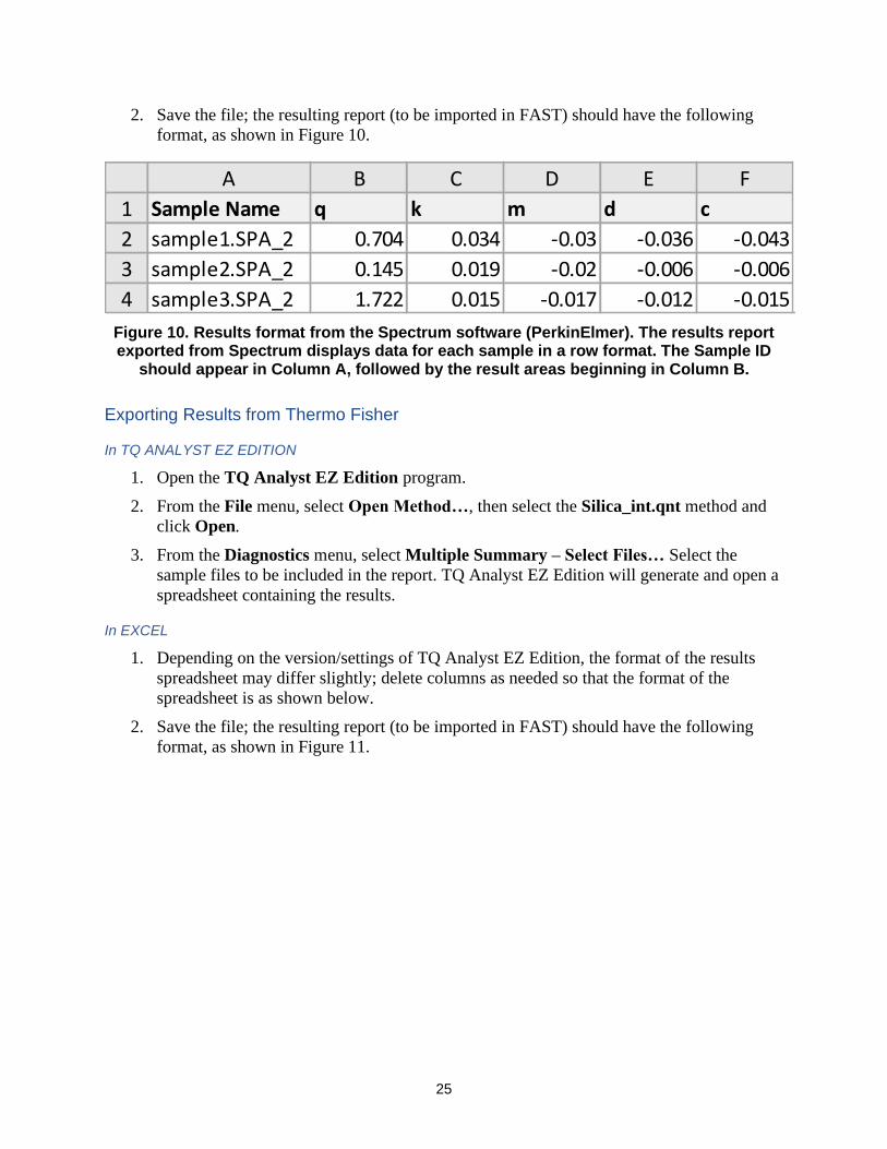
2. Save the file; the resulting report (to be imported in FAST) should have the following
format, as shown in Figure 11.
26
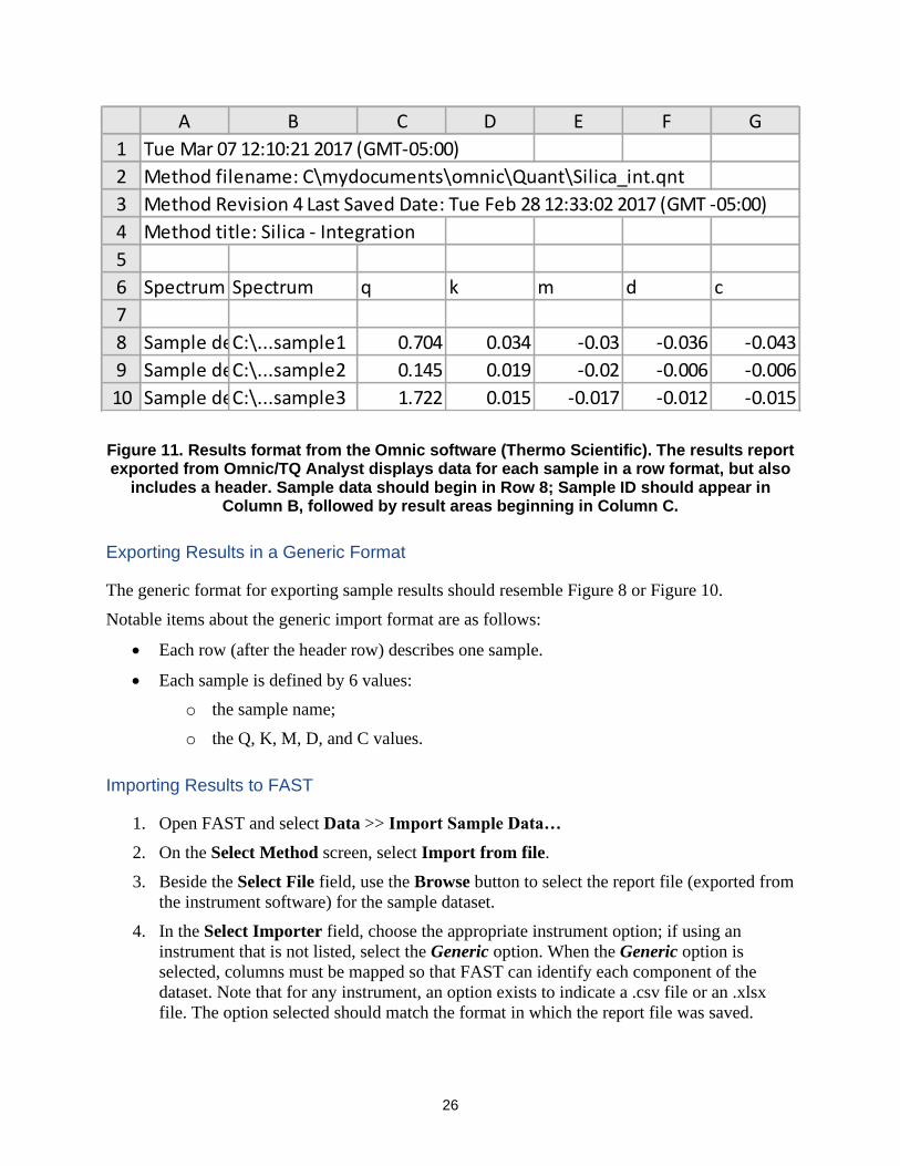
Figure 11. Results format from the Omnic software (Thermo Scientific). The results report exported from Omnic/TQ Analyst displays data for each sample in a row format, but also
includes a header. Sample data should begin in Row 8; Sample ID should appear in Column B, followed by result areas beginning in Column C.
A B C D E F G
1 Tue Mar 07 12:10:21 2017 (GMT-05:00)
2 Method filename: C\mydocuments\omnic\Quant\Silica_int.qnt
3 Method Revision 4 Last Saved Date: Tue Feb 28 12:33:02 2017 (GMT -05:00)
4 Method title: Silica - Integration
5
6 Spectrum Spectrum q k m d c
7
8 Sample descriptionC:\...sample1 0.704 0.034 -0.03 -0.036 -0.043
9 Sample descriptionC:\...sample2 0.145 0.019 -0.02 -0.006 -0.006
10 Sample descriptionC:\...sample3 1.722 0.015 -0.017 -0.012 -0.015
Exporting Results in a Generic Format
The generic format for exporting sample results should resemble Figure 8 or Figure 10.
Notable items about the generic import format are as follows:
• Each row (after the header row) describes one sample.
• Each sample is defined by 6 values:
o the sample name;
o the Q, K, M, D, and C values.
Importing Results to FAST
1. Open FAST and select Data >> Import Sample Data…
2. On the Select Method screen, select Import from file.
3. Beside the Select File field, use the Browse button to select the report file (exported from
the instrument software) for the sample dataset.
4. In the Select Importer field, choose the appropriate instrument option; if using an
instrument that is not listed, select the Generic option. When the Generic option is
selected, columns must be mapped so that FAST can identify each component of the
dataset. Note that for any instrument, an option exists to indicate a .csv file or an .xlsx
file. The option selected should match the format in which the report file was saved.
27
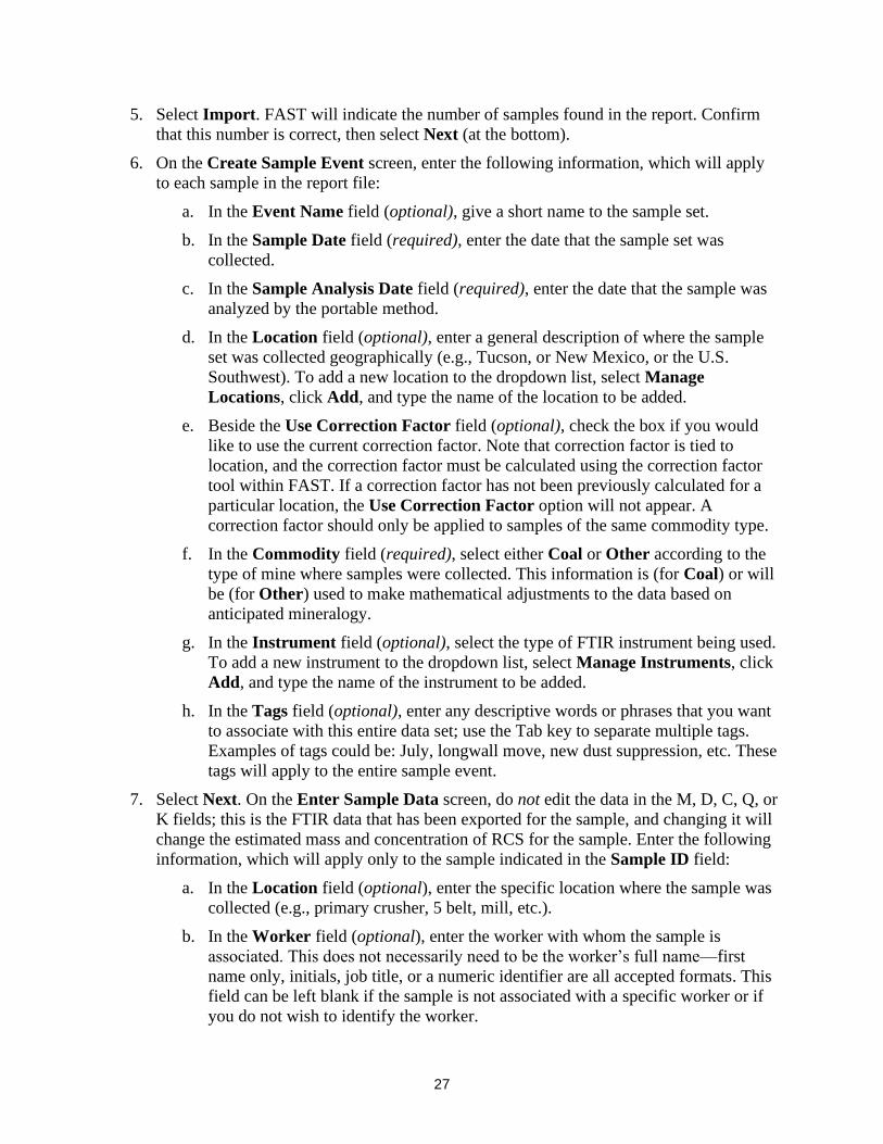
5. Select Import. FAST will indicate the number of samples found in the report. Confirm
that this number is correct, then select Next (at the bottom).
6. On the Create Sample Event screen, enter the following information, which will apply
to each sample in the report file:
a. In the Event Name field (optional), give a short name to the sample set.
b. In the Sample Date field (required), enter the date that the sample set was
collected.
c. In the Sample Analysis Date field (required), enter the date that the sample was
analyzed by the portable method.
d. In the Location field (optional), enter a general description of where the sample
set was collected geographically (e.g., Tucson, or New Mexico, or the U.S.
Southwest). To add a new location to the dropdown list, select Manage
Locations, click Add, and type the name of the location to be added.
e. Beside the Use Correction Factor field (optional), check the box if you would
like to use the current correction factor. Note that correction factor is tied to
location, and the correction factor must be calculated using the correction factor
tool within FAST. If a correction factor has not been previously calculated for a
particular location, the Use Correction Factor option will not appear. A
correction factor should only be applied to samples of the same commodity type.
f. In the Commodity field (required), select either Coal or Other according to the
type of mine where samples were collected. This information is (for Coal) or will
be (for Other) used to make mathematical adjustments to the data based on
anticipated mineralogy.
g. In the Instrument field (optional), select the type of FTIR instrument being used.
To add a new instrument to the dropdown list, select Manage Instruments, click
Add, and type the name of the instrument to be added.
h. In the Tags field (optional), enter any descriptive words or phrases that you want
to associate with this entire data set; use the Tab key to separate multiple tags.
Examples of tags could be: July, longwall move, new dust suppression, etc. These
tags will apply to the entire sample event.
7. Select Next. On the Enter Sample Data screen, do not edit the data in the M, D, C, Q, or
K fields; this is the FTIR data that has been exported for the sample, and changing it will
change the estimated mass and concentration of RCS for the sample. Enter the following
information, which will apply only to the sample indicated in the Sample ID field:
a. In the Location field (optional), enter the specific location where the sample was
collected (e.g., primary crusher, 5 belt, mill, etc.).
b. In the Worker field (optional), enter the worker with whom the sample is
associated. This does not necessarily need to be the worker’s full name—first
name only, initials, job title, or a numeric identifier are all accepted formats. This
field can be left blank if the sample is not associated with a specific worker or if
you do not wish to identify the worker.
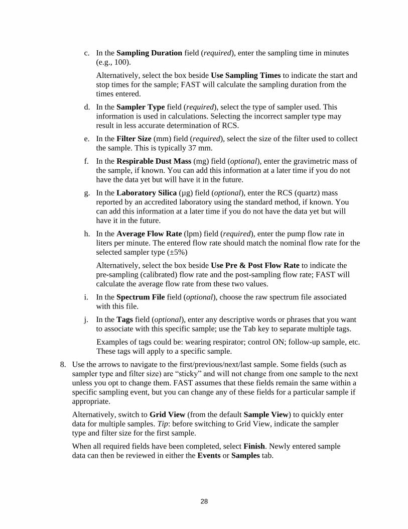
28
c. In the Sampling Duration field (required), enter the sampling time in minutes
(e.g., 100).
Alternatively, select the box beside Use Sampling Times to indicate the start and
stop times for the sample; FAST will calculate the sampling duration from the
times entered.
d. In the Sampler Type field (required), select the type of sampler used. This
information is used in calculations. Selecting the incorrect sampler type may
result in less accurate determination of RCS.
e. In the Filter Size (mm) field (required), select the size of the filter used to collect
the sample. This is typically 37 mm.
f. In the Respirable Dust Mass (mg) field (optional), enter the gravimetric mass of
the sample, if known. You can add this information at a later time if you do not
have the data yet but will have it in the future.
g. In the Laboratory Silica (µg) field (optional), enter the RCS (quartz) mass
reported by an accredited laboratory using the standard method, if known. You
can add this information at a later time if you do not have the data yet but will
have it in the future.
h. In the Average Flow Rate (lpm) field (required), enter the pump flow rate in
liters per minute. The entered flow rate should match the nominal flow rate for the
selected sampler type (±5%)
Alternatively, select the box beside Use Pre & Post Flow Rate to indicate the
pre-sampling (calibrated) flow rate and the post-sampling flow rate; FAST will
calculate the average flow rate from these two values.
i. In the Spectrum File field (optional), choose the raw spectrum file associated
with this file.
j. In the Tags field (optional), enter any descriptive words or phrases that you want
to associate with this specific sample; use the Tab key to separate multiple tags.
Examples of tags could be: wearing respirator; control ON; follow-up sample, etc.
These tags will apply to a specific sample.
8. Use the arrows to navigate to the first/previous/next/last sample. Some fields (such as
sampler type and filter size) are “sticky” and will not change from one sample to the next
unless you opt to change them. FAST assumes that these fields remain the same within a
specific sampling event, but you can change any of these fields for a particular sample if
appropriate.
Alternatively, switch to Grid View (from the default Sample View) to quickly enter
data for multiple samples. Tip: before switching to Grid View, indicate the sampler
type and filter size for the first sample.
When all required fields have been completed, select Finish. Newly entered sample
data can then be reviewed in either the Events or Samples tab.
29
Supporting Field-based Analysis for Respirable Crystalline Silica
Keeping a Logbook
It is important to keep detailed and accurate records of the analyses that have been completed as
well as notes indicating quality assurance measures. This is particularly helpful in situations
where multiple people are using the instrument, or the instrument is used infrequently by the
same person.
To maintain an accurate record of what has been done, a logbook entry should be recorded every
time that the instrument is used. Suggested information to include is as follows:
• Date
• Name or initials of the analyst
• Whether instrument checks were performed
• Result of instrument checks (if performed)
• Which QA samples were analyzed
• Results of QA sample checks
• Any anomalies related to the QA sample check or the QA samples themselves
• Other anomalies during analysis
• Details identifying the sample set
• Location of saved sample report
A typical logbook entry might look like the example shown in Figure 12.
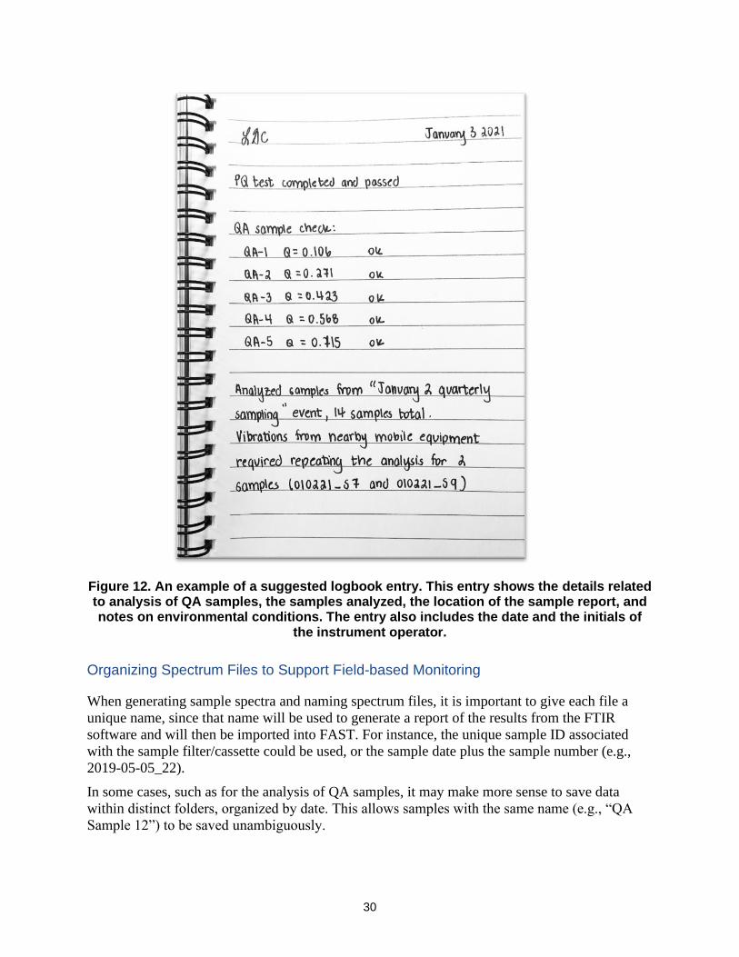
30
Figure 12. An example of a suggested logbook entry. This entry shows the details related to analysis of QA samples, the samples analyzed, the location of the sample report, and notes on environmental conditions. The entry also includes the date and the initials of
the instrument operator.
Organizing Spectrum Files to Support Field-based Monitoring
When generating sample spectra and naming spectrum files, it is important to give each file a
unique name, since that name will be used to generate a report of the results from the FTIR
software and will then be imported into FAST. For instance, the unique sample ID associated
with the sample filter/cassette could be used, or the sample date plus the sample number (e.g.,
2019-05-05_22).
In some cases, such as for the analysis of QA samples, it may make more sense to save data
within distinct folders, organized by date. This allows samples with the same name (e.g., “QA
Sample 12”) to be saved unambiguously.
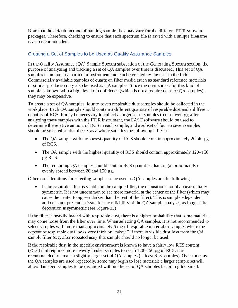
31
Note that the default method of naming sample files may vary for the different FTIR software
packages. Therefore, checking to ensure that each spectrum file is saved with a unique filename
is also recommended.
Creating a Set of Samples to be Used as Quality Assurance Samples
In the Quality Assurance (QA) Sample Spectra subsection of the Generating Spectra section, the
purpose of analyzing and tracking a set of QA samples over time is discussed. This set of QA
samples is unique to a particular instrument and can be created by the user in the field.
Commercially available samples of quartz on filter media (such as standard reference materials
or similar products) may also be used as QA samples. Since the quartz mass for this kind of
sample is known with a high level of confidence (which is not a requirement for QA samples),
they may be expensive.
To create a set of QA samples, four to seven respirable dust samples should be collected in the
workplace. Each QA sample should contain a different quantity of respirable dust and a different
quantity of RCS. It may be necessary to collect a larger set of samples (ten to twenty); after
analyzing these samples with the FTIR instrument, the FAST software should be used to
determine the relative amount of RCS in each sample, and a subset of four to seven samples
should be selected so that the set as a whole satisfies the following criteria:
• The QA sample with the lowest quantity of RCS should contain approximately 20–40 µg
of RCS.
• The QA sample with the highest quantity of RCS should contain approximately 120–150
µg RCS.
• The remaining QA samples should contain RCS quantities that are (approximately)
evenly spread between 20 and 150 µg.
Other considerations for selecting samples to be used as QA samples are the following:
• If the respirable dust is visible on the sample filter, the deposition should appear radially
symmetric. It is not uncommon to see more material at the center of the filter (which may
cause the center to appear darker than the rest of the filter). This is sampler-dependent
and does not present an issue for the reliability of the QA sample analysis, as long as the
deposition is symmetric (see Figure 13).
If the filter is heavily loaded with respirable dust, there is a higher probability that some material
may come loose from the filter over time. When selecting QA samples, it is not recommended to
select samples with more than approximately 5 mg of respirable material or samples where the
deposit of respirable dust looks very thick or “cakey.” If there is visible dust loss from the QA
sample filter (e.g. after repeated use), that sample should no longer be used.
If the respirable dust in the specific environment is known to have a fairly low RCS content
(<5%) that requires more heavily loaded samples to reach 120–150 µg of RCS, it is
recommended to create a slightly larger set of QA samples (at least 6–8 samples). Over time, as
the QA samples are used repeatedly, some may begin to lose material; a larger sample set will
allow damaged samples to be discarded without the set of QA samples becoming too small.
32
Figure 13. Illustration of the deposition of material in respirable dust samples. Many samplers result in a visible concentration of material at the center of the filter compared to the edge of the filter. This is not a problem, provided that the deposit is centered on
the filter (left) rather than skewed towards the edge of the filter (right).
Generating a Site-specific Correction Factor
The quality of the quantification of RCS in respirable dust samples using the portable direct-on-
filter FTIR approach can be affected by the presence of other minerals in the samples [Foster and
Walker 1984; Ojima 2003; Pickard et al. 1985; Taylor et al. 1970]. Accredited laboratories have
the experience and knowledge to address this issue during the FTIR analysis and the processing
of the data as indicated by NIOSH method 7603 [NIOSH 2017b], which adopts the FTIR
technique for RCS analysis. In addition, the NIOSH 7603 method provides guidance for sample
preparation procedures that can reduce the presence of certain minerals.
Most users of the field-based method will likely not have the same level of experience as a
laboratory infrared spectroscopy expert and, for this reason, quantification models have been
developed to standardize the RCS quantification in the presence of confounding minerals.
Specific quantification models have been designed for samples collected in coal mines.
For samples collected in any environment designated in the FAST software as “other” (which
includes non-mining environments, FAST does not include tailored quantification models.
Additional tailored quantification models may be added in future updates to FAST. Until that
time, a different strategy—the “site-specific quantification model”—can be used to address the
presence of mineral interferences. As the name suggests, the site-specific quantification model
uses a correction factor that is unique to a particular site. A site can be one or several workplace
environments (within the same operation) where it is reasonable to assume that the
characteristics of the respirable dust (including percent quartz content) are similar. Qualitative
information (such as the color of the respirable dust on the sample filters), quantitative
information (such as the percent silica reported by the external laboratory for previous samples
collected in an area), and operational information (such as knowledge of processes that use
additives or chemical that could also be present in the dust sample) can be used to determine if
two areas are similar enough to be considered the same site.
33
Ultimately, a site is determined at the user’s discretion. For example, a small quarry operation,
including the pit, the plant, and the lab, might be considered a single site if the respirable dust
has a similar appearance and quartz content throughout. A large multi-pit metal mine might
encompass several different sites (i.e. each pit, each processing area, and the lab) if respirable
dust has different characteristics depending on the area of the operation. In certain situations,
such as in industries including construction or manufacturing, correction factors that are unique
to specific tasks could be used instead (e.g., a correction factor specific to cutting brick and a
correction factor specific to breaking concrete). Publications describe the application of this
method [Cauda et al. 2018; Hart et al. 2018].
Regardless of how big or small a site is, the correction factor for that site should be periodically
evaluated via laboratory analysis. This evaluation should include samples from all areas of the
facility to which the correction factor is applied; the ratio of the result of the field-based analysis
to the results of the lab-based analysis should be approximately the same for all samples. For any
samples where this ratio is different, a unique correction factor should be generated and used.
To generate a site-specific quantification model, the procedure outlined below should be
followed.
1. Collect a set of at least fifteen to twenty samples. The sample set should contain a range
of respirable dust loadings. The final sample set should contain at least ten samples,
ranging from 20–30 µg RCS per sample to 275–325 µg RCS per sample, which may be
determined using either the direct-on-filter approach or the standard analysis through an
off-site laboratory. Ideally, sample loadings will be (approximately) evenly spread
between 20 and 325 µg of RCS. While a total respirable dust loading can be estimated
from expected concentration and sampling time, it can be difficult to estimate the RCS
loading accurately in this way, so additional samples are recommended. Gravimetric
analysis (such as NIOSH 0600 [NIOSH 1998]), if available, may be helpful. These
guidelines are summarized within the Calculate Correction Factor function of the
FAST software.
2. Analyze the samples using the FTIR instrument and import the data into FAST. At this
point, choose which samples will remain in the sample set and which will be excluded
(i.e., if they are outside of the loading range; if they are duplicates or extras). When
importing the data into FAST, be sure to indicate the location for which you plan to use
the correction factor.
3. Submit the sample set to an off-site laboratory for the standard RCS analysis.
4. When the sample results are received from the laboratory, add each laboratory result to
the appropriate sample in FAST by right clicking on a sample, selecting “edit,” and
adding the result to the Laboratory Silica field.
5. To calculate the correction factor, select Calculate Correction Factor from the Data
menu in FAST. Select the appropriate event location. FAST will display samples that
may be used to calculate the correction factor; it will not display samples for which
laboratory results are not available, or samples outside of the range of 20–325 µg RCS.
Click on samples to select them; at least 10 samples must be selected. Use the “Data
Quality Evaluation Results” at the bottom of the screen (see Figure 14) to guide you as
you select the samples to include; the correction factor generated with the currently
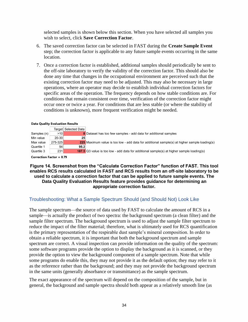
34
selected samples is shown below this section. When you have selected all samples you
wish to select, click Save Correction Factor.
6. The saved correction factor can be selected in FAST during the Create Sample Event
step; the correction factor is applicable to any future sample events occurring in the same
location.
7. Once a correction factor is established, additional samples should periodically be sent to
the off-site laboratory to verify the validity of the correction factor. This should also be
done any time that changes in the occupational environment are perceived such that the
existing correction factor may need to be adjusted. This may also be necessary in large
operations, where an operator may decide to establish individual correction factors for
specific areas of the operation. The frequency depends on how stable conditions are. For
conditions that remain consistent over time, verification of the correction factor might
occur once or twice a year. For conditions that are less stable (or where the stability of
conditions is unknown), more frequent verification might be needed.
Figure 14. Screenshot from the “Calculate Correction Factor” function of FAST. This tool enables RCS results calculated in FAST and RCS results from an off-site laboratory to be
used to calculate a correction factor that can be applied to future sample events. The Data Quality Evaluation Results feature provides guidance for determining an
appropriate correction factor.
Troubleshooting: What a Sample Spectrum Should (and Should Not) Look Like
The sample spectrum—the source of data used by FAST to calculate the amount of RCS in a
sample—is actually the product of two spectra: the background spectrum (a clean filter) and the
sample filter spectrum. The background spectrum is used to adjust the sample filter spectrum to
reduce the impact of the filter material; therefore, what is ultimately used for RCS quantification
is the primary representation of the respirable dust sample’s mineral composition. In order to
obtain a reliable spectrum, it is important that both the background spectrum and sample
spectrum are correct. A visual inspection can provide information on the quality of the spectrum:
some software programs provide the option to display the background as it is scanned, or they
provide the option to view the background component of a sample spectrum. Note that while
some programs do enable this, they may not provide it as the default option; they may refer to it
as the reference rather than the background; and they may not provide the background spectrum
in the same units (generally absorbance or transmittance) as the sample spectrum.
The exact appearance of the spectrum will depend on the composition of the sample, but in
general, the background and sample spectra should both appear as a relatively smooth line (as
35
opposed to a “spiky” line with many abrupt changes), especially in the right-hand side (also
known as the fingerprint region) of the spectrum (closer to 600 cm-1). Depending on the
instrument or the software, there may be a region of “noisy” data on the left-hand side (closer to
4000 cm-1); as long as the noise is relatively consistent from day to day and does not occur to the
right of approximately 3000 cm-1, this is acceptable. If noise suddenly increases or appears in an
area that previously was not noisy, this indicates that a problem needs to be addressed before
continuing to analyze samples.
Figure 15 shows images of both good background and sample spectra, while Figure 16 shows
examples of spectra with varying distortions and noise levels. Although sample spectra will all
be slightly different (depending on how much material the sample contains and its composition),
most will have similar qualities, and over time, many users will be able to readily distinguish a
high quality sample spectrum from one of lower quality. These examples are intended to
facilitate that but should not be considered comprehensive of all the spectra or issues that may
arise. Note that spectra have not been baseline-corrected in Figures 15 and 16, except where
noted.
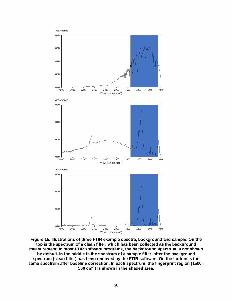
36
Figure 15. Illustrations of three FTIR example spectra, background and sample. On the top is the spectrum of a clean filter, which has been collected as the background
measurement. In most FTIR software programs, the background spectrum is not shown by default. In the middle is the spectrum of a sample filter, after the background
spectrum (clean filter) has been removed by the FTIR software. On the bottom is the same spectrum after baseline correction. In each spectrum, the fingerprint region (1500–
500 cm-1) is shown in the shaded area.
0.00
0.10
0.20
0.30
0.40
40080012001600200024002800320036004000
Absorbance
Wavenumber (cm-1)
0.00
0.10
0.20
0.30
40080012001600200024002800320036004000
Absorbance
Wavenumber (cm-1)
0.00
0.10
0.20
0.30
40080012001600200024002800320036004000
Absorbance
Wavenumber (cm-1)
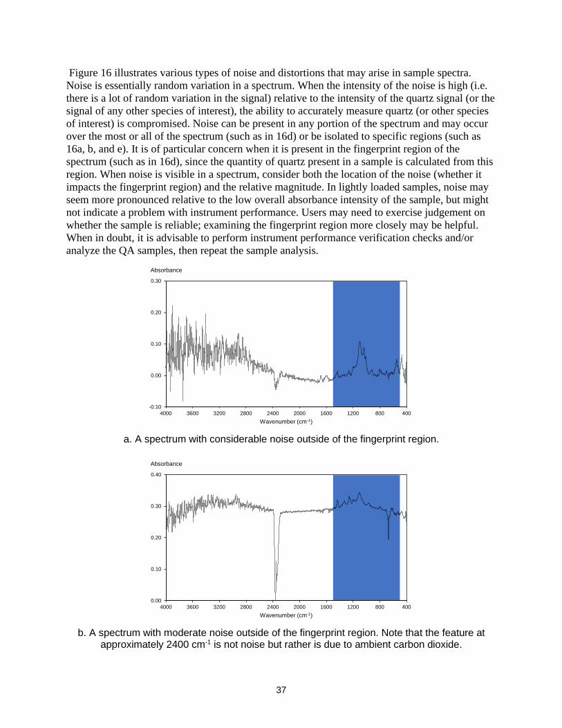
37
Figure 16 illustrates various types of noise and distortions that may arise in sample spectra.
Noise is essentially random variation in a spectrum. When the intensity of the noise is high (i.e.
there is a lot of random variation in the signal) relative to the intensity of the quartz signal (or the
signal of any other species of interest), the ability to accurately measure quartz (or other species
of interest) is compromised. Noise can be present in any portion of the spectrum and may occur
over the most or all of the spectrum (such as in 16d) or be isolated to specific regions (such as
16a, b, and e). It is of particular concern when it is present in the fingerprint region of the
spectrum (such as in 16d), since the quantity of quartz present in a sample is calculated from this
region. When noise is visible in a spectrum, consider both the location of the noise (whether it
impacts the fingerprint region) and the relative magnitude. In lightly loaded samples, noise may
seem more pronounced relative to the low overall absorbance intensity of the sample, but might
not indicate a problem with instrument performance. Users may need to exercise judgement on
whether the sample is reliable; examining the fingerprint region more closely may be helpful.
When in doubt, it is advisable to perform instrument performance verification checks and/or
analyze the QA samples, then repeat the sample analysis.
a. A spectrum with considerable noise outside of the fingerprint region.
-0.10
0.00
0.10
0.20
0.30
40080012001600200024002800320036004000
Absorbance
Wavenumber (cm-1)
b. A spectrum with moderate noise outside of the fingerprint region. Note that the feature at approximately 2400 cm-1 is not noise but rather is due to ambient carbon dioxide.
0.00
0.10
0.20
0.30
0.40
40080012001600200024002800320036004000
Absorbance
Wavenumber (cm-1)
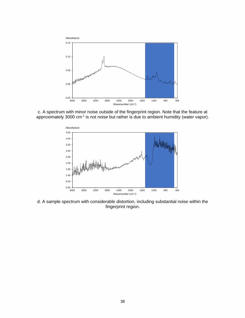
38
c. A spectrum with minor noise outside of the fingerprint region. Note that the feature at approximately 3000 cm-1 is not noise but rather is due to ambient humidity (water vapor).
-0.05
0.00
0.05
0.10
0.15
40080012001600200024002800320036004000
Absorbance
Wavenumber (cm-1)
d. A sample spectrum with considerable distortion, including substantial noise within the fingerprint region.
0.00
0.50
1.00
1.50
2.00
2.50
3.00
3.50
4.00
4.50
40080012001600200024002800320036004000
Absorbance
Wavenumber (cm-1)
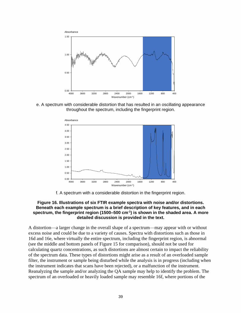
39
e. A spectrum with considerable distortion that has resulted in an oscillating appearance throughout the spectrum, including the fingerprint region.
0.00
0.50
1.00
1.50
40080012001600200024002800320036004000
Absorbance
Wavenumber (cm-1)
f. A spectrum with a considerable distortion in the fingerprint region.
0.00
0.50
1.00
1.50
2.00
2.50
3.00
3.50
4.00
4.50
40080012001600200024002800320036004000
Absorbance
Wavenumber (cm-1)
Figure 16. Illustrations of six FTIR example spectra with noise and/or distortions. Beneath each example spectrum is a brief description of key features, and in each
spectrum, the fingerprint region (1500–500 cm-1) is shown in the shaded area. A more detailed discussion is provided in the text.
A distortion—a larger change in the overall shape of a spectrum—may appear with or without
excess noise and could be due to a variety of causes. Spectra with distortions such as those in
16d and 16e, where virtually the entire spectrum, including the fingerprint region, is abnormal
(see the middle and bottom panels of Figure 15 for comparison), should not be used for
calculating quartz concentrations, as such distortions are almost certain to impact the reliability
of the spectrum data. These types of distortions might arise as a result of an overloaded sample
filter, the instrument or sample being disturbed while the analysis is in progress (including when
the instrument indicates that scans have been rejected), or a malfunction of the instrument.
Reanalyzing the sample and/or analyzing the QA sample may help to identify the problem. The
spectrum of an overloaded or heavily loaded sample may resemble 16f, where portions of the
40
spectrum appear normal but the tops of some of the peaks in the fingerprint region are distorted.
This happens when there is so much sample that the instrument detector is “overwhelmed” by
the sample signal.
Note that peaks at approximately 2400 cm-1 and 3000 cm-1 (see Figure 16b and 16c, respectively)
are not noise but are normal features due to ambient carbon dioxide and water vapor,
respectively. These peaks may be more prominent, less prominent, or even absent depending on
sample loading and how similar the ambient conditions are when the background is scanned and
when the sample is scanned.
Possible Causes of Spectrum Problems
A number of causes might be responsible for spectrum problems, as described below, followed
by their solutions.
Problem: Incorrect sample analysis settings.
Solution: Check that all the sample analysis parameters match those in Table 1; correct any
settings that do not match.
Problem: Background spectrum is faulty.
Solution: Re-scan; choose a different clean filter if necessary.
Problem: Unsuitable analysis conditions (heavy vibrations, sample bracket is loose, sample is
moving during analysis, etc.)
Solution: Make sure that the bracket and sample holder are secure so that the sample is
stationary when analysis begins. Light vibration is typically not an issue if it is steady but may be
problematic if it is intermittent during analysis. If vibrations are present, place the instrument on
a sturdy surface (such as a heavy desk) or wait until vibrations decrease.
Problem: Instrument windows are smudged, dirty, cloudy, or cracked.
Solution: Clean or replace windows. Note that windows are very difficult to clean without
smudging or scratching; therefore it is recommended to replace dirty windows (and store the
instrument so that dust and humidity are minimized).
Problem: Other hardware issue.
Solution: Run instrument diagnostics to determine the problem; consult software help
documentation or the instrument manufacturer to repair/replace hardware.
Selecting the Appropriate Sampler Type in FAST
The sampler used to collect the dust sample for direct-on-filter analysis has an important role in
the analytical approach. The choice of sampler must ensure that the collected sample is
representative of respirable dust in the environment monitored. The sampler also affects the
quantification model for RCS and the appropriate sampler must be selected in the FAST software
in order for the RCS result to be accurate.
41
As described in the previous sections, this specific direct-on-filter approach entails the analysis
of a small portion of the dust sample deposited on the filter. This portion is a circular area
approximately 6–9 mm in diameter in the center of the filter. The quantification of RCS is then
calculated by using established quantification models to correlate the analysis in the center of the
filter with the quantity of RCS present on the entire filter. The quantification model is a function
of how the dust sample is distributed across the filter, or the deposition pattern of respirable dust
on the filter.
Respirable dust particles enter a sampling cassette as an aerosol in a stream of air (see Figure 17,
top). Once inside the cassette, the aerosol is distributed throughout the volume of the cassette
while moving towards the filter media. Eventually, the dust particles are collected on the filter
and the air stream exits the cassette. Several factors affect the aerodynamic behavior of the
aerosol inside the cassette and, ultimately, the deposition pattern of the dust on the filter: the air
velocity at the inlet of the cassette, residence time of the air inside the cassette, the shape of the
cassette, and the sampler outlet. The combination of these factors induces different deposition
patterns of the dust on filter. The size of the filter also has an influence on the deposition pattern:
most samplers collect respirable dust on 37-mm-diameter filters, although some samplers use
25mm or 47-mm diameter filters.
Examples of deposition patterns induced by two samplers/cassettes configurations (see Figure
17, bottom) are presented here. Both samplers use 37-mm diameter filters, which are the most
common type used in the United States. Note that the figure refers to the nylon Dorr-Oliver
sampler with a luer fitting; the conductive style of this sampler and the nylon version with
coupler will result in samples with similar but not identical patterns of dust deposition.
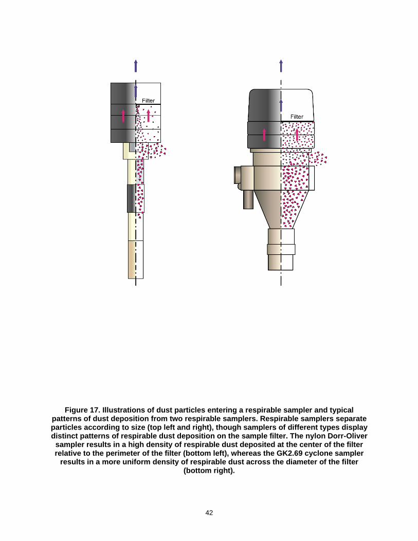
42
Figure 17. Illustrations of dust particles entering a respirable sampler and typical patterns of dust deposition from two respirable samplers. Respirable samplers separate particles according to size (top left and right), though samplers of different types display distinct patterns of respirable dust deposition on the sample filter. The nylon Dorr-Oliver
sampler results in a high density of respirable dust deposited at the center of the filter relative to the perimeter of the filter (bottom left), whereas the GK2.69 cyclone sampler
results in a more uniform density of respirable dust across the diameter of the filter (bottom right).
43
The two samplers are the GK2.69 cyclone (BGI by Mesa Labs, Butler, NJ) [Stacey et al. 2014;
Stacey et al. 2013] and the 10-mm nylon Dorr-Oliver cyclone (Zefon International, Ocala, FL)
[Lidén and Kenny 1993; Maynard 1993; Bartley et al. 2010]. The GK2.69 sampler is operated at
a flow rate of 4.2 lpm for respirable dust collection; the Dorr-Oliver sampler is operated at a flow
rate of 1.7 lpm except when it is used in U.S. coal mines, where it is used at 2.0 lpm as specified
in 30 CFR 70.205 [2019]. The GK2.69 sampler is coupled with a 37-mm diameter cassette in a
configuration called an “open-face cassette,” in which the aerosol exits the sampler directly into
the volume of the cassette. In contrast, the Dorr-Oliver sampler uses an enclosed cassette and the
aerosol moves from the sampler to the cassette through a narrow coupler. Because of these
differences and the factors presented above, the deposition pattern for respirable dust samples
collected by the two samplers is different. The respirable dust particles collected with the
GK2.69 sampler are spread evenly across the 37-mm diameter filter. The respirable dust particles
collected with the DO sampler tend to be more concentrated in the center of the filter than at the
edges. Both deposition patterns have been found to be consistent for a wide range of respirable
dust (and RCS) loadings.
Note that electrostatic effects can adversely affect the sample (changes to sample deposition,
increased wall losses, etc.). Samples collected using samplers and cassettes that are composed of
conductive or static-dissipative materials are less susceptible to these effects than samples
collected using more insulating materials [NIOSH 2016a]. In general, the minimization of wall
losses is preferred for direct-on-filter analysis, since only the material deposited on the filter can
be analyzed by the instrument.
How Deposition Pattern Affects the Quantification for Respirable Crystalline Silica Using the Direct-on-filter Analysis
The deposition pattern influences the relationship between the area in the center of the filter that
is analyzed directly by the FTIR and the remaining portion of the sample that is not analyzed by
the FTIR. Different deposition patterns translate into different models for quantification of RCS
on the entire filter. In other words, two samples may contain the same mass of RCS, but the raw
FTIR results would be different if they were collected with different samplers. For this reason,
the quantification model for the sampler used to collect the sample needs to be used for the
quantification of RCS in the sample. In FAST, selecting the correct sampler type will ensure that
the quantification model developed for that sampler is used.
NIOSH has developed quantification models for samples collected with a number of commonly
used samplers which have been incorporated into FAST. NIOSH is working on developing
additional quantification models for samples collected with other samplers. Once the models for
additional types of samplers have been developed, they will be added to the FAST software.
“Housekeeping” Suggestions for FTIR Instruments
Because the use of the FTIR instrument at a site might be intermittent, several housekeeping
suggestions are recommended for optimum performance, as follows.
Once an instrument is set up and operating, it may be left powered on for several days (or longer)
between analysis sessions; leaving the instrument on is preferable to frequently turning it on and
off. When the instrument will not be used for an extended period of time (several weeks or
44
more), it is strongly recommended to store the instrument in a protective case and to store the
case in a suitable environment. If the conditions of the storage environment (especially
temperature and humidity) are different from the environment where the instrument will be used,
the instrument should be allowed to equilibrate with the new environment for at least 24 hours
before it is powered on. This helps to ensure that any condensation has time to dissipate, as this
could harm the internal electrical components of the instrument.
Note that the performance of an FTIR instrument relies on internal optical components. In some
instruments, some of the optical components are partially exposed and can be affected or
damaged by dirt and humidity if care is not taken. Best practices include keeping the lid or door
to the transmission compartment closed when the instrument is not actively being used and
exercising care not to touch or disturb internal components when the transmission compartment
is opened to insert or remove a sample.
Environment for Storage and Use of FTIR Instruments
The environment where the FTIR instrument is stored and where it is operated should be as
described below. Note that while FTIR instruments may be used to analyze samples collected in
an underground environment, the instruments themselves are not intended for underground use
and should only be used in above-ground environments.
Low in Humidity
Storage: If storing the instrument in a low-humidity environment is not possible, the FTIR
instrument should be stored in an airtight container (such as a large, sealed bag) with a desiccant
(such as a silica gel pack) to absorb excess moisture.
Operation: Most instruments can operate in up to 80% non-condensing humidity; however, high
humidity will degrade some components over time, negatively impacting data quality and
eventually requiring replacement.
Moderate in Temperature
Temperature should be between approximately 18°C and 35°C (65°F and 95°F).
Relatively Clean and Free of Dust
Storage: If storing the instrument in a clean environment is not possible, the FTIR instrument
should be stored in an airtight container (such as a large, sealed bag).
Operation: While small amounts of dust are generally not harmful, larger quantities can
contaminate samples and may begin to accumulate in the FTIR instrument sample chamber and
potentially in internal chambers, which could negatively impact data quality or cause equipment
damage over time. A site office or a similar location is generally suitable; cleaning the work
surface with a damp cloth before setting up the instrument can also help to control dust.
Not Prone to Physical Disturbances
Storage: Prolonged periods of physical disturbance (such as vibrations from nearby heavy
equipment) are a concern. While short-duration vibrations and small bumps should not affect the
instrument, prolonged movement may loosen or misalign internal components.
45
Operation: Sudden shocks or vibrations are a concern. While occasional moderate vibrations are
not likely to harm the instrument, they can affect the data quality.
Guidelines for Performing Standard Laboratory Analysis on Samples Analyzed in the Field
This section provides basic guidance on when it may be advantageous to conduct laboratory
analysis on samples that have already been analyzed in the field with the portable FTIR, using
methods such as MSHA P-2 [MSHA 2013a], MSHA P-7 [MSHA 2013b], NIOSH 7500 [NIOSH
2003], NIOSH 7603 [NIOSH 2017b], and OSHA ID-142 [OSHA 2015]. Because the laboratory
analysis is an additional cost (per sample) that the operator must account for, it is important to
use this option strategically.
Because of its nature as direct-on-filter, non-destructive analysis, field-based RCS monitoring
does not degrade the dust samples, which allows users to analyze the same samples with the
standard analysis as well if desired. This can be done by submitting the samples to an off-site
accredited laboratory. The possibility of conducting laboratory analysis on the same samples
analyzed in the field is an important feature of the monitoring approach and is an option that
users should consider to maximize the impact of this tool. When field-based RCS monitoring is
implemented initially, new users may find it helpful to have the same-sample comparison of
field-based results and laboratory results for a majority of samples. This approach can be used to
confirm that users are acquiring reliable results, as well as to determine if a single site-specific
correction factor is appropriate for an operation, or if different correction factors would be
appropriate for different work areas. As more experience is gained with field-based monitoring,
laboratory analysis does not necessarily need to be conducted on all samples. Instead, laboratory
analysis can be conducted periodically on specific sample sets to 1) confirm overall reliability of
field-based analysis (including when new personnel become involved in field-based monitoring,
when a new instrument is acquired or when an old instrument is serviced, or when an instrument
has not been used for an extended period of time), 2) check site-specific correction factors, and
3) compose reports where laboratory accredited data is required.
The FAST software has been designed to allow users to add laboratory results to existing
samples in the FAST database. The user can edit the “laboratory mass (µg)” field to add
laboratory RCS results for each sample at any time. In addition, the user can also edit the
“respirable dust mass (mg)” for the same sample. These data are available from the laboratory
results. In this way, the user can have a comprehensive set of results from the field and
laboratory on the same sample, with the data all stored together in FAST.
At the time this document was published, direct-on-filter analysis with portable FTIR was not a
stand-alone NIOSH analytical method or a standard analytical method used by MSHA or OSHA
or other international bodies. For this reason, when there is a need for a formal assessment of
compliance status, the dust samples analyzed in the field should then be sent to an accredited
laboratory. In this case, the role of field-based monitoring should be to act in support of
maintaining regulatory compliance. The goal is that the faster, more comprehensive assessment
of the RCS exposure levels that is facilitated by the use of field-based monitoring should
increase the probability of compliance status for the operator and protection of workers. This is
accomplished by decreasing the RCS concentration and exposure, which is the primary goal of
the monitoring approach.
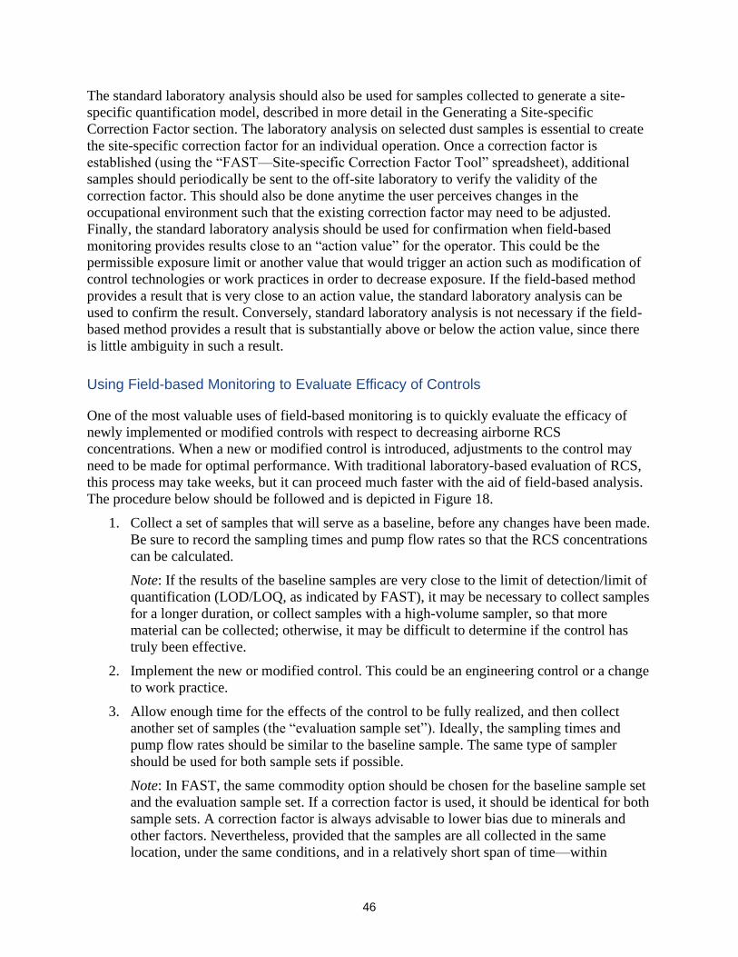
46
The standard laboratory analysis should also be used for samples collected to generate a site-
specific quantification model, described in more detail in the Generating a Site-specific
Correction Factor section. The laboratory analysis on selected dust samples is essential to create
the site-specific correction factor for an individual operation. Once a correction factor is
established (using the “FAST—Site-specific Correction Factor Tool” spreadsheet), additional
samples should periodically be sent to the off-site laboratory to verify the validity of the
correction factor. This should also be done anytime the user perceives changes in the
occupational environment such that the existing correction factor may need to be adjusted.
Finally, the standard laboratory analysis should be used for confirmation when field-based
monitoring provides results close to an “action value” for the operator. This could be the
permissible exposure limit or another value that would trigger an action such as modification of
control technologies or work practices in order to decrease exposure. If the field-based method
provides a result that is very close to an action value, the standard laboratory analysis can be
used to confirm the result. Conversely, standard laboratory analysis is not necessary if the field-
based method provides a result that is substantially above or below the action value, since there
is little ambiguity in such a result.
Using Field-based Monitoring to Evaluate Efficacy of Controls
One of the most valuable uses of field-based monitoring is to quickly evaluate the efficacy of
newly implemented or modified controls with respect to decreasing airborne RCS
concentrations. When a new or modified control is introduced, adjustments to the control may
need to be made for optimal performance. With traditional laboratory-based evaluation of RCS,
this process may take weeks, but it can proceed much faster with the aid of field-based analysis.
The procedure below should be followed and is depicted in Figure 18.
1. Collect a set of samples that will serve as a baseline, before any changes have been made.
Be sure to record the sampling times and pump flow rates so that the RCS concentrations
can be calculated.
Note: If the results of the baseline samples are very close to the limit of detection/limit of
quantification (LOD/LOQ, as indicated by FAST), it may be necessary to collect samples
for a longer duration, or collect samples with a high-volume sampler, so that more
material can be collected; otherwise, it may be difficult to determine if the control has
truly been effective.
2. Implement the new or modified control. This could be an engineering control or a change
to work practice.
3. Allow enough time for the effects of the control to be fully realized, and then collect
another set of samples (the “evaluation sample set”). Ideally, the sampling times and
pump flow rates should be similar to the baseline sample. The same type of sampler
should be used for both sample sets if possible.
Note: In FAST, the same commodity option should be chosen for the baseline sample set
and the evaluation sample set. If a correction factor is used, it should be identical for both
sample sets. A correction factor is always advisable to lower bias due to minerals and
other factors. Nevertheless, provided that the samples are all collected in the same
location, under the same conditions, and in a relatively short span of time—within
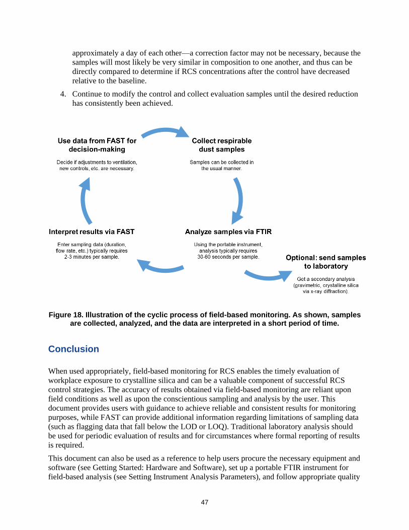
47
approximately a day of each other—a correction factor may not be necessary, because the
samples will most likely be very similar in composition to one another, and thus can be
directly compared to determine if RCS concentrations after the control have decreased
relative to the baseline.
4. Continue to modify the control and collect evaluation samples until the desired reduction
has consistently been achieved.
Figure 18. Illustration of the cyclic process of field-based monitoring. As shown, samples are collected, analyzed, and the data are interpreted in a short period of time.
Conclusion
When used appropriately, field-based monitoring for RCS enables the timely evaluation of
workplace exposure to crystalline silica and can be a valuable component of successful RCS
control strategies. The accuracy of results obtained via field-based monitoring are reliant upon
field conditions as well as upon the conscientious sampling and analysis by the user. This
document provides users with guidance to achieve reliable and consistent results for monitoring
purposes, while FAST can provide additional information regarding limitations of sampling data
(such as flagging data that fall below the LOD or LOQ). Traditional laboratory analysis should
be used for periodic evaluation of results and for circumstances where formal reporting of results
is required.
This document can also be used as a reference to help users procure the necessary equipment and
software (see Getting Started: Hardware and Software), set up a portable FTIR instrument for
field-based analysis (see Setting Instrument Analysis Parameters), and follow appropriate quality

48
assurance procedures (see Verifying Instrument Integrity; Creating a Set of Samples to be Used
as Quality Assurance Samples; and Keeping a Logbook). Appendix A contains links to
additional resources that can be used in the field-based monitoring process, Appendix B contains
checklists to guide users through the most vital field-based monitoring procedures, and Appendix
C contains comparisons of several FTIR analysis methods and parameters discussed in this
document.
49
References
Code of Federal Regulations [2019]. Sampling procedures: Approved sampling devices;
operation; air flowrate. 30 CFR 70.205.
Ashley E, Cauda E, Chubb LG, Tuchman DP, Rubinstein EN [2020]. Performance comparison
of four portable FTIR instruments for direct-on-filter measurement of respirable crystalline
silica. Ann Work Expo Health, https://doi.org/10.1093/annweh/wxaa031.
Bartley DL, Chen C-C, Song R, Fischbach TJ [2010]. Respirable aerosol sampler performance
testing. AIHAJ 55(11):1036–1046, https://doi.org/10.1080/15428119491018303.
Cauda E, Chubb L, Reed R, Stepp R [2018]. Evaluating the use of a field-based silica monitoring
approach with dust from copper mines. J Occup Environ Hyg 15(10):732–742,
https://doi.org/10.1080/15459624.2018.1495333.
Cauda E, Miller A, Drake P [2016]. Promoting early exposure monitoring for respirable
crystalline silica: Taking the laboratory to the mine site. J Occup Environ Hyg 13(3):D39–45,
https://www.ncbi.nlm.nih.gov/pubmed/26558490.
Foster RD, Walker RF [1984]. Quantitative determination of crystalline silica in respirable-size
dust samples by infrared spectrophotometry. Analyst 109:1117–1127,
https://doi.org/10.1039/AN9840901117.
Harris G, Maguire B [1968]. A gravimetric dust sampling instrument (SIMPEDS): Preliminary
results. Ann Occup Hyg 11:195–201, https://doi.org/10.1093/annhyg/11.3.195.
Hart JF, Autenrieth DA, Cauda E, Chubb L, Spear TM, Wock S, Rosenthal S [2018]. A
comparison of respirable crystalline silica concentration measurements using a direct-on-filter
Fourier transform infrared (FT-IR) transmission method versus a traditional laboratory X-ray
diffraction method. J Occup Environ Hyg 15(10):743–754,
https://doi.org/10.1080/15459624.2018.1495334.
Lee T, Lee L, Cauda E, Hummer J, Harper M [2017]. Respirable size-selective sampler for end-
of-shift quartz measurement: Development and performance. J Occup Environ Hyg 14(5):335–
342, https://doi.org/10.1080/15459624.2016.1252845.
Lidén G, Kenny LC [1993]. Optimization of the performance of existing respirable dust
samplers. Appl Occup Environ Hyg 8(4):386–391,
https://doi.org/10.1080/1047322x.1993.10389224.
Maynard AD [1993]. Respirable dust sampler characterisation: Efficiency curve reproducibility.
J Aerosol Sci 24:S457–S458, https://doi.org/10.1016/0021-8502(93)90321-Y.
Miller AL, Drake PL, Murphy NC, Cauda E, LeBouf R, Markevicius G [2013]. Deposition
uniformity of coal dust on filters and its effect on the accuracy of FTIR analyses for silica.
Aerosol Sci Technol, https://doi.org/10.1080/02786826.2013.787157.
Miller AL, Drake PL, Murphy NC, Noll JD, Volkwein JC [2012]. Evaluating portable infrared
spectrometers for measuring the silica content of coal dust. J Environ Monit 14(1):48–55,
http://dx.doi.org/10.1039/C1EM10678C.
50
MSHA [2013a]. Method P2 X-ray diffraction determination of quartz and cristobalite in
respirable mine dust. https://arlweb.msha.gov/Techsupp/pshtcweb/MSHA%20P2.pdf.
MSHA [2013b]. Method P7 Infrared determination of quartz in respirable coal mine dust.
https://arlweb.msha.gov/Techsupp/pshtcweb/MSHA%20P7.pdf.
NIOSH [1998]. Method 0600 Particulates not otherwise regulated, respirable. NIOSH Manual of
Analytical Methods, Fourth Edition, https://www.cdc.gov/niosh/docs/2003-154/pdfs/0600.pdf.
NIOSH [2002]. NIOSH hazard review: health effects of occupational exposure to respirable
crystalline silica. Publication No. 2002-129. Cincinnati, OH: National Institute for Occupational
Safety and Health, https://www.cdc.gov/niosh/docs/2002-
129/pdfs/2002129.pdf?id=10.26616/NIOSHPUB2002129.
NIOSH [2003a]. Chapter R: Determination of Airborne Crystalline Silica. NIOSH Manual of
Analytical Methods, Fourth Edition, https://www.cdc.gov/niosh/docs/2003-
154/pdfs/chapterr.pdf.
NIOSH [2003b]. Method 7500 Silica, crystalline, by XRD (filter redeposition) NIOSH Manual
of Analytical Methods, Fourth Edition, https://www.cdc.gov/niosh/docs/2003-154/pdfs/7500.pdf.
NIOSH [2016a]. Chapter AE: Factors affecting aerosol sampling. NIOSH Manual of Analytical
Methods, Fifth Edition, https://www.cdc.gov/niosh/docs/2014-151/pdfs/chapters/chapter-ae.pdf.
NIOSH [2016b]. Chapter SA: General considerations for sampling airborne contaminants.
NIOSH Manual of Analytical Methods, Fifth Edition,
https://www.cdc.gov/niosh/docs/2014151/pdfs/chapters/chapter-sa.pdf.
NIOSH [2017a]. Method 7602 Silica, crystalline by IR (KBr pellet). NIOSH Manual of
Analytical Methods, Fifth Edition, https://www.cdc.gov/niosh/nmam/pdf/7602.pdf.
NIOSH [2017b]. Method 7603 Quartz in coal mine dust, by IR (redeposition). NIOSH Manual of
Analytical Methods, Fifth Edition, https://www.cdc.gov/niosh/nmam/pdf/7603.pdf.
Ojima J [2003]. Determining of crystalline silica in respirable dust samples by infrared
spectrophotometry in the presence of interferences. J Occup Health 45:94–103,
https://doi.org/10.1539/joh.45.94.
OSHA [2015]. Method ID-142 Crystalline silica, quartz and cristobalite.
https://www.osha.gov/dts/sltc/methods/inorganic/id142/id142.pdf.
Pampena J, Cauda E, Chubb L, Meadows J [2019]. Use of the field-based silica monitoring
technique in a coal mine: a case study. Min Metall Explor, https://doi.org/10.1007/s42461-
01900161-0.
Pickard KJ, Walker RF, West NG [1985]. A comparison of X-ray diffraction and infrared
spectrophotometric methods for the analysis of alpha-quartz in airborne dusts. Ann Occup Hyg
29(2):149–167, https://doi.org/10.1093/annhyg/29.2.149.
Stacey P, Lee T, Thorpe A, Roberts P, Frost G, Harper M [2014]. Collection efficiencies of high
flow rate personal respirable samplers when measuring Arizona road dust and analysis of quartz
by x-ray diffraction. Ann Occup Hyg 58(4):512–523, https://doi.org/10.1093/annhyg/met075.

51
Stacey P, Mecchia M, Verpaele S, Pretorius C, Key-Schwartz R, Mattenklott M, Eypert-Blaison
C, Thorpe A, Roberts P, Frost G [2013]. Differences between samplers for respirable dust and
the analysis of quartz—an international study, In: Silica and Associated Respirable Mineral
Particles, STP 1565, ed. by Harper M, Lee T, West Conshohocken, PA: ASTM International, pp.
73–102.
Taylor DG, Nenadic CM, Crable JV [1970]. Infrared spectra for mineral identification. AIHAJ
31(1):100–108, https://doi.org/10.1080/0002889708506215.
52
Appendix A: Additional Resources for Field-based Monitoring
Listed below are tools that can support and facilitate field-based monitoring. Some tools are used
in conjunction with the instrument software; several versions are available to accommodate
different software packages. Other tools are independent of the instrument software and the same
version can be utilized by any user.
All of the following resources are freely available online.
Software-specific Resources (https://github.com/niosh-mining/fast/)
• Experiment setup files (see Table 2)
• Macros for spectral processing
• Report templates
General resources (https://github.com/niosh-mining/fast/)
• QA Sample Tracking spreadsheet
3D Model Files (https://3dprint.nih.gov/)
• Sample bracket (instrument-specific)
• Sample cradle (for use with the four-piece cassette)
• Sample holder (for use with dust sampling cassette)
• Prototype respirable sampler (see Lee et al. 2017)
Additional guidance for using the provided 3D Model Files:
• The 3D Models available from the link above were designed for a fused deposition
modeling (FDM) layer thickness of 0.005 inches when using acrylonitrile butadiene
styrene (ABS) material. Different materials and printer formats can affect the accuracy of
the printed model, and these specifications should be used as a benchmark. For instance:
o An FDM layer thickness of 0.015 inches or greater will have a cross section with
edges that appear amplified in their rounded coarseness. Printer manufacturers try
to compensate for an amount of layer flow, but much is dependent on local
conditions.
o A printer utilizing a cured liquid deposition may exhibit a much finer edge section
resulting in greater accuracy.
• Note that the models are provided in units of inches; users who typically print in metric
units should be mindful of the conversion.
• Consider how the item is oriented relative to the printer head or nozzle as it is being
printed. Generally, the accuracy of the sample cradle, either as a full or half circle, will be
greater when oriented perpendicular to the printing head, and greater accuracy will be
achieved when the part is printed lying flat on the print platen.
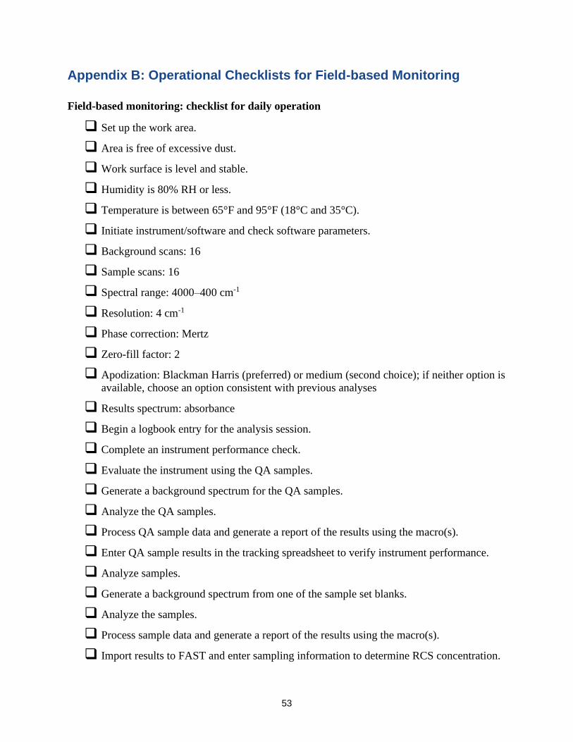
53
Appendix B: Operational Checklists for Field-based Monitoring
Field-based monitoring: checklist for daily operation
❑ Set up the work area.
❑ Area is free of excessive dust.
❑ Work surface is level and stable.
❑ Humidity is 80% RH or less.
❑ Temperature is between 65°F and 95°F (18°C and 35°C).
❑ Initiate instrument/software and check software parameters.
❑ Background scans: 16
❑ Sample scans: 16
❑ Spectral range: 4000–400 cm-1
❑ Resolution: 4 cm-1
❑ Phase correction: Mertz
❑ Zero-fill factor: 2
❑ Apodization: Blackman Harris (preferred) or medium (second choice); if neither option is
available, choose an option consistent with previous analyses
❑ Results spectrum: absorbance
❑ Begin a logbook entry for the analysis session.
❑ Complete an instrument performance check.
❑ Evaluate the instrument using the QA samples.
❑ Generate a background spectrum for the QA samples.
❑ Analyze the QA samples.
❑ Process QA sample data and generate a report of the results using the macro(s).
❑ Enter QA sample results in the tracking spreadsheet to verify instrument performance.
❑ Analyze samples.
❑ Generate a background spectrum from one of the sample set blanks.
❑ Analyze the samples.
❑ Process sample data and generate a report of the results using the macro(s).
❑ Import results to FAST and enter sampling information to determine RCS concentration.
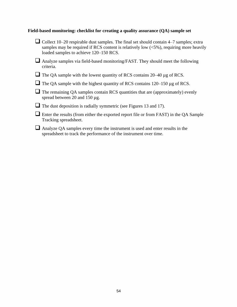
54
Field-based monitoring: checklist for creating a quality assurance (QA) sample set
❑ Collect 10–20 respirable dust samples. The final set should contain 4–7 samples; extra
samples may be required if RCS content is relatively low (<5%), requiring more heavily
loaded samples to achieve 120–150 RCS.
❑ Analyze samples via field-based monitoring/FAST. They should meet the following
criteria.
❑ The QA sample with the lowest quantity of RCS contains 20–40 µg of RCS.
❑ The QA sample with the highest quantity of RCS contains 120–150 µg of RCS.
❑ The remaining QA samples contain RCS quantities that are (approximately) evenly
spread between 20 and 150 µg.
❑ The dust deposition is radially symmetric (see Figures 13 and 17).
❑ Enter the results (from either the exported report file or from FAST) in the QA Sample
Tracking spreadsheet.
❑ Analyze QA samples every time the instrument is used and enter results in the
spreadsheet to track the performance of the instrument over time.
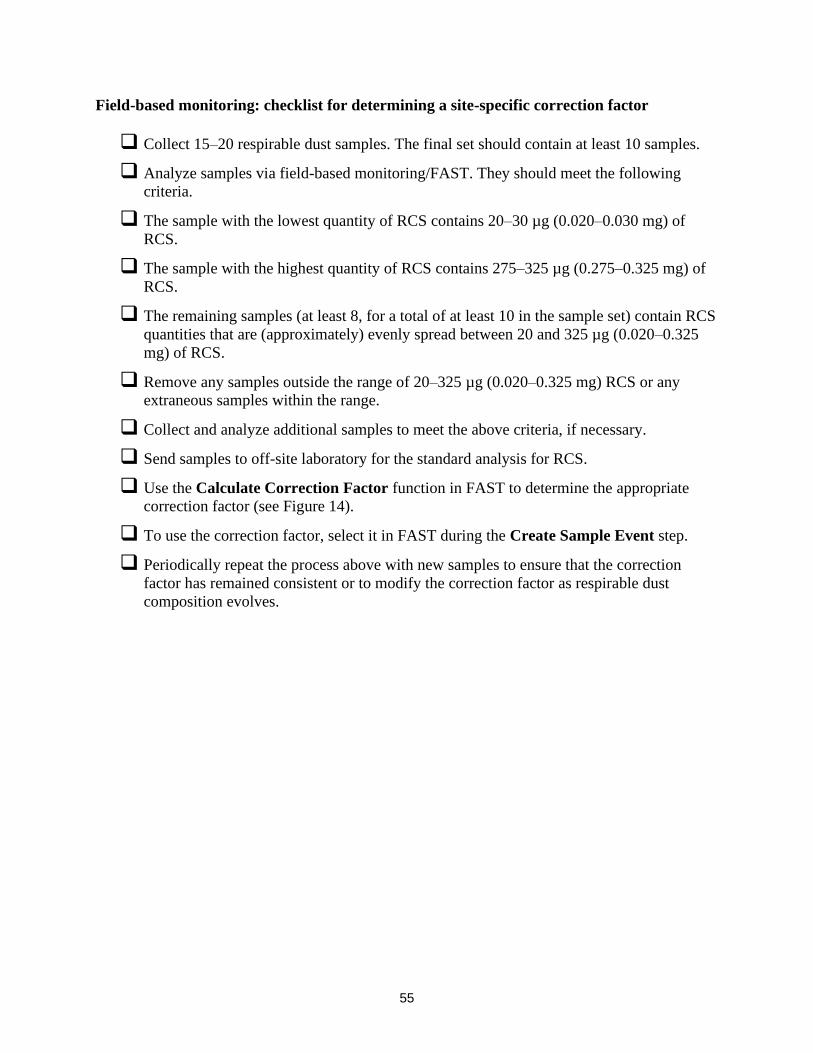
55
Field-based monitoring: checklist for determining a site-specific correction factor
❑ Collect 15–20 respirable dust samples. The final set should contain at least 10 samples.
❑ Analyze samples via field-based monitoring/FAST. They should meet the following
criteria.
❑ The sample with the lowest quantity of RCS contains 20–30 µg (0.020–0.030 mg) of
RCS.
❑ The sample with the highest quantity of RCS contains 275–325 µg (0.275–0.325 mg) of
RCS.
❑ The remaining samples (at least 8, for a total of at least 10 in the sample set) contain RCS
quantities that are (approximately) evenly spread between 20 and 325 µg (0.020–0.325
mg) of RCS.
❑ Remove any samples outside the range of 20–325 µg (0.020–0.325 mg) RCS or any
extraneous samples within the range.
❑ Collect and analyze additional samples to meet the above criteria, if necessary.
❑ Send samples to off-site laboratory for the standard analysis for RCS.
❑ Use the Calculate Correction Factor function in FAST to determine the appropriate
correction factor (see Figure 14).
❑ To use the correction factor, select it in FAST during the Create Sample Event step.
❑ Periodically repeat the process above with new samples to ensure that the correction
factor has remained consistent or to modify the correction factor as respirable dust
composition evolves.
56
Appendix C: Comparison of FTIR data obtained using different methods or parameters
As discussed in the Generating Spectra section, there are two methods for generating a
background spectrum, and as summarized in Table 2, there are several available options for
instrument software settings such as apodization and baseline correction. The tables in this
appendix illustrate the differences that could be expected in sample results for several common
options for these settings.
Note that differences seen in actual samples for these types of settings may be greater or less
than the differences shown here for laboratory prepared samples. Tables C1, C2, and C4 show
data for samples containing only quartz to illustrate a “best case scenario”, while Tables C3 and
C5 show data for samples that are approximately 25% quartz, in addition to other mineral phases
(such as albite/anorthite, microcline, phlogopite, and clinochlore) in order to illustrate a more
complex sample. Since different mineral phases can have different impacts on sample spectra
and actual samples may be even more complex, these results should not be considered
representative of every potential composition of respirable dust that might be encountered.
Regardless of the composition of samples or the settings chosen, it is important to use the same
settings consistently, rather than switching between different settings for different samples.
How the samples for Tables C1, C2, and C4 were collected and analyzed:
The following procedures were used to collect this data with a portable FTIR instrument with the
parameters shown in Table 2:
1. Clean PVC filters were first analyzed by FTIR, using the empty sample compartment
(ambient air) as the background scan.
2. Samples of a high purity quartz material (Minusil 5) were collected on the filters using
the Dorr-Oliver nylon cyclone, operated at a flow rate of 1.7 lpm. The mass of quartz
collected ranged from approximately 15 µg to 300 µg of quartz crystalline silica.
3. Sample filters were then analyzed again by FTIR, again using the empty sample
compartment (ambient air) as the background scan.
a. From each sample spectrum, the initial spectrum of the clean filter (from Step 1)
was subtracted.
b. The macro procedure was used to perform a baseline correction (concave
rubberband correction) and calculate the peak area for quartz, and the FAST
software was then used to estimate the silica mass. These data are reported in the
right column of Table C1.
4. Sample filters were analyzed once more by FTIR, using a clean filter (from the same
lot as the rest of the sample filters) as the background scan.
a. The macro procedure was used to perform a baseline correction (concave
rubberband correction) and calculate the peak area for quartz, and the FAST
software (with “other” for the selected commodity and using no correction
factor) was then used to estimate the silica mass. These data are reported in the
left column of Table C1, Table C2, and Table C4.
57
5. The original sample spectra from Step 4 (before the macro procedure was applied)
were reprocessed to assess differences in results for three apodization options:
a. Original spectra were converted from Blackman Harris 3 term apodization to
medium apodization. The macro procedure was used on the new spectra to
perform a baseline correction (concave rubberband correction) and calculate the
peak area for quartz, and the FAST software was then used to estimate the silica
mass. These data are reported in the center column of Table C2.
b. Original spectra were converted from Blackman Harris 3 term apodization to
boxcar apodization. The macro procedure was used on the new spectra to
perform a baseline correction (concave rubberband correction) and calculate the
peak area for quartz, and the FAST software was then used to estimate the silica
mass. These data are reported in the right column of Table C2.
6. The original sample spectra from Step 4 (before the macro procedure was applied)
were reprocessed to assess differences in results for four baseline correction options.
Note that while the macro procedure itself was not used here (since the macro
procedure includes a concave rubberband baseline correction), the equivalent steps
were performed each time (a baseline correction followed by calculating the peak
area for quartz).
a. Original sample spectra were baseline corrected using a scattering baseline
correction, the peak area for quartz was calculated, and the FAST software was
then used to estimate the silica mass. These data are reported in the second from
the left column of Table C4.
b. Original sample spectra were baseline corrected using a rubberband baseline
correction, the peak area for quartz was calculated, and the FAST software was
then used to estimate the silica mass. These data are reported in the second from
the right column of Table C4.
c. The peak area for quartz was calculated from the original sample spectra with no
baseline correction, and the FAST software was then used to estimate the silica
mass. These data are reported in the right column of Table C4.
How the samples for Tables C3 and C5 were collected and analyzed:
1. Samples of a material from a granite quarry (approximately 25% quartz) were
collected on PVC filters using the Dorr-Oliver nylon cyclone, operated at a flow rate
of 1.7 lpm. The total mass of respirable dust collected ranged from approximately 100
µg to 1700 µg (approximately 30 to 400 µg quartz).
2. Sample filters were analyzed by FTIR, using a clean filter as the background scan.
a. The macro procedure was used to perform a baseline correction (concave
rubberband correction) and calculate the peak area for quartz, and the FAST
software was then used to estimate the silica mass. These data are reported in the
left column of Tables C3 and C5.
58
3. The original sample spectra from Step 2 (before the macro procedure was applied)
were reprocessed to assess differences in results for three apodization options:
a. Original spectra were converted from Blackman Harris 3-term apodization to
medium apodization. The macro procedure was used on the new spectra to
perform a baseline correction (concave rubberband correction) and calculate the
peak area for quartz, and the FAST software was then used to estimate the silica
mass. These data are reported in the center column of Table C3.
b. Original spectra were converted from Blackman Harris 3-term apodization to
boxcar apodization. The macro procedure was used on the new spectra to
perform a baseline correction (concave rubberband correction) and calculate the
peak area for quartz, and the FAST software was then used to estimate the silica
mass. These data are reported in the right column of Table C3.
4. The original sample spectra from Step 2 (before the macro procedure was applied)
were reprocessed to assess differences in results for four baseline correction options.
Note that while the macro procedure was not used here (since the macro procedure
includes a concave rubberband baseline correction), the equivalent steps were
performed each time (a baseline correction followed by calculating the peak area for
quartz).
a. Original sample spectra were baseline corrected using a scattering baseline
correction, the peak area for quartz was calculated, and the FAST software was
then used to estimate the silica mass. These data are reported in the second from
the left column of Table C5.
b. Original sample spectra were baseline corrected using a rubberband baseline
correction, the peak area for quartz was calculated, and the FAST software was
then used to estimate the silica mass. These data are reported in the second from
the right column of Table C5.
c. The peak area for quartz was calculated from the original sample spectra with no
baseline correction, and the FAST software was then used to estimate the silica
mass. These data are reported in the right column of Table C5.
Comparing the two methods for background scans
Table C1 shows a comparison of estimated quartz mass for the same sample filter containing
only quartz, using two different methods for the background (as described above and in the
Generating Spectra section). For these samples, differences in results between the two methods
range from 0–10 µg RCS, with a mean difference of 3 µg.
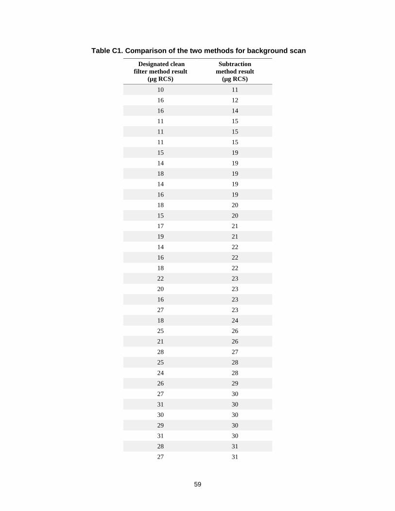
59
Table C1. Comparison of the two methods for background scan
Designated clean
filter method result
(µg RCS)
Subtraction
method result
(µg RCS)
10 11
16 12
16 14
11 15
11 15
11 15
15 19
14 19
18 19
14 19
16 19
18 20
15 20
17 21
19 21
14 22
16 22
18 22
22 23
20 23
16 23
27 23
18 24
25 26
21 26
28 27
25 28
24 28
26 29
27 30
31 30
30 30
29 30
31 30
28 31
27 31
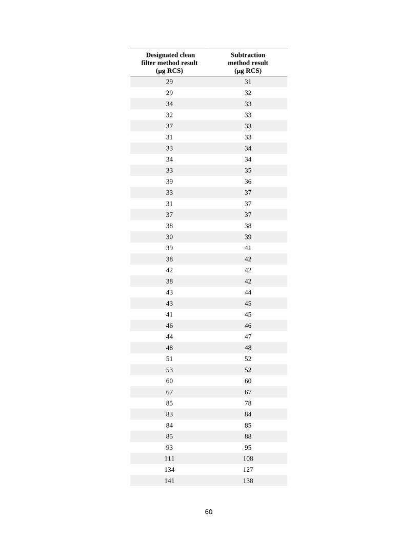
60
Designated clean
filter method result
(µg RCS)
Subtraction
method result
(µg RCS)
29 31
29 32
34 33
32 33
37 33
31 33
33 34
34 34
33 35
39 36
33 37
31 37
37 37
38 38
30 39
39 41
38 42
42 42
38 42
43 44
43 45
41 45
46 46
44 47
48 48
51 52
53 52
60 60
67 67
85 78
83 84
84 85
85 88
93 95
111 108
134 127
141 138
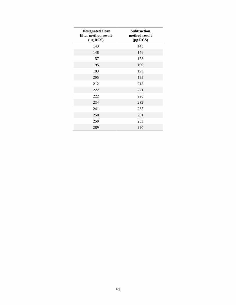
61
Designated clean
filter method result
(µg RCS)
Subtraction
method result
(µg RCS)
143 143
148 148
157 158
195 190
193 193
205 195
212 212
222 221
222 228
234 232
241 235
250 251
250 253
289 290
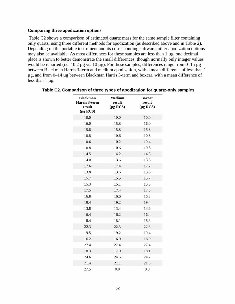
62
Comparing three apodization options
Table C2 shows a comparison of estimated quartz mass for the same sample filter containing
only quartz, using three different methods for apodization (as described above and in Table 2).
Depending on the portable instrument and its corresponding software, other apodization options
may also be available. As most differences for these samples are less than 1 µg, one decimal
place is shown to better demonstrate the small differences, though normally only integer values
would be reported (i.e. 10.2 µg vs. 10 µg). For these samples, differences range from 0–15 µg
between Blackman Harris 3-term and medium apodization, with a mean difference of less than 1
µg, and from 0–14 µg between Blackman Harris 3-term and boxcar, with a mean difference of
less than 1 µg.
Table C2. Comparison of three types of apodization for quartz-only samples
Blackman
Harris 3-term
result
(µg RCS)
Medium
result
(µg RCS)
Boxcar
result
(µg RCS)
10.0 10.0 10.0
16.0 15.8 16.0
15.8 15.8 15.8
10.8 10.6 10.8
10.6 10.2 10.4
10.8 10.6 10.8
14.5 14.2 14.3
14.0 13.6 13.8
17.6 17.4 17.7
13.8 13.6 13.8
15.7 15.5 15.7
15.3 15.1 15.3
17.5 17.4 17.5
16.8 16.6 16.8
19.4 19.2 19.4
13.8 13.4 13.6
16.4 16.2 16.4
18.4 18.1 18.3
22.3 22.3 22.3
19.5 19.2 19.4
16.2 16.0 16.0
27.4 27.4 27.4
18.3 17.9 18.1
24.6 24.5 24.7
21.4 21.1 21.3
27.5 0.0 0.0
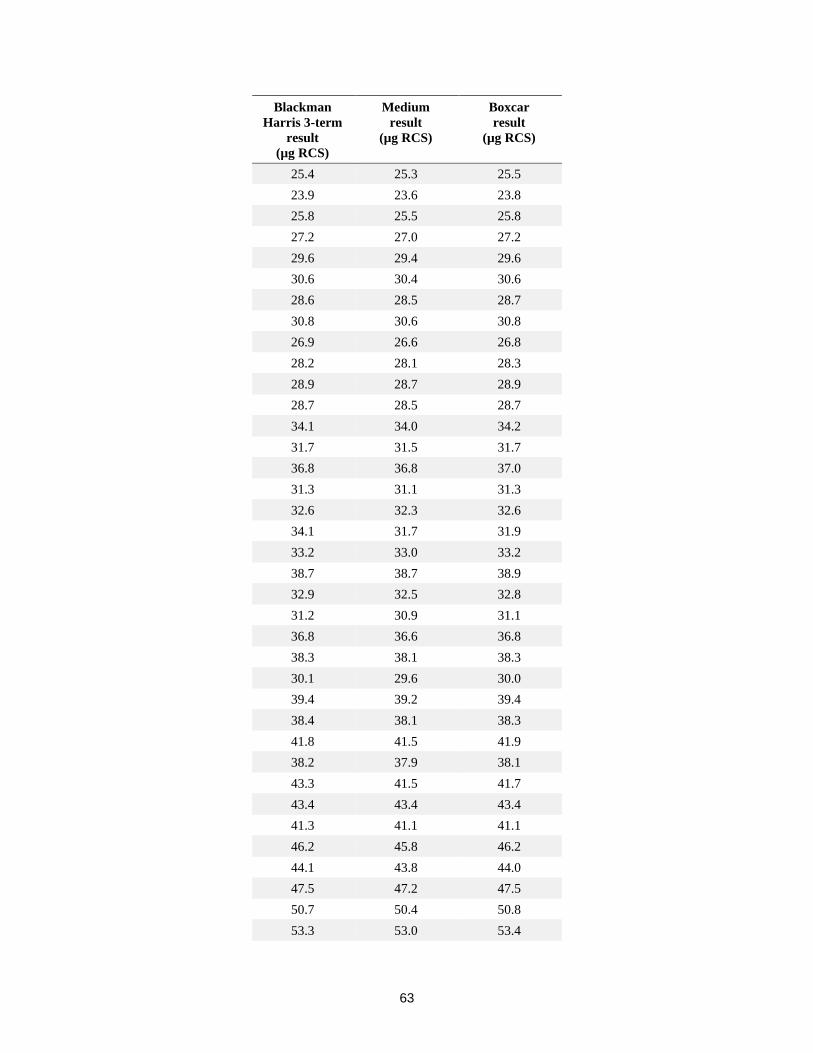
63
Blackman
Harris 3-term
result
(µg RCS)
Medium
result
(µg RCS)
Boxcar
result
(µg RCS)
25.4 25.3 25.5
23.9 23.6 23.8
25.8 25.5 25.8
27.2 27.0 27.2
29.6 29.4 29.6
30.6 30.4 30.6
28.6 28.5 28.7
30.8 30.6 30.8
26.9 26.6 26.8
28.2 28.1 28.3
28.9 28.7 28.9
28.7 28.5 28.7
34.1 34.0 34.2
31.7 31.5 31.7
36.8 36.8 37.0
31.3 31.1 31.3
32.6 32.3 32.6
34.1 31.7 31.9
33.2 33.0 33.2
38.7 38.7 38.9
32.9 32.5 32.8
31.2 30.9 31.1
36.8 36.6 36.8
38.3 38.1 38.3
30.1 29.6 30.0
39.4 39.2 39.4
38.4 38.1 38.3
41.8 41.5 41.9
38.2 37.9 38.1
43.3 41.5 41.7
43.4 43.4 43.4
41.3 41.1 41.1
46.2 45.8 46.2
44.1 43.8 44.0
47.5 47.2 47.5
50.7 50.4 50.8
53.3 53.0 53.4
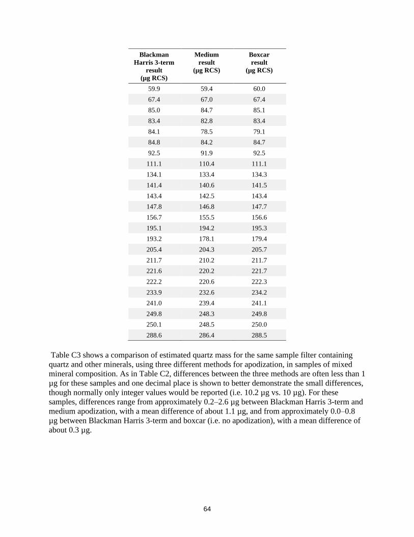
64
Blackman
Harris 3-term
result
(µg RCS)
Medium
result
(µg RCS)
Boxcar
result
(µg RCS)
59.9 59.4 60.0
67.4 67.0 67.4
85.0 84.7 85.1
83.4 82.8 83.4
84.1 78.5 79.1
84.8 84.2 84.7
92.5 91.9 92.5
111.1 110.4 111.1
134.1 133.4 134.3
141.4 140.6 141.5
143.4 142.5 143.4
147.8 146.8 147.7
156.7 155.5 156.6
195.1 194.2 195.3
193.2 178.1 179.4
205.4 204.3 205.7
211.7 210.2 211.7
221.6 220.2 221.7
222.2 220.6 222.3
233.9 232.6 234.2
241.0 239.4 241.1
249.8 248.3 249.8
250.1 248.5 250.0
288.6 286.4 288.5
Table C3 shows a comparison of estimated quartz mass for the same sample filter containing
quartz and other minerals, using three different methods for apodization, in samples of mixed
mineral composition. As in Table C2, differences between the three methods are often less than 1
µg for these samples and one decimal place is shown to better demonstrate the small differences,
though normally only integer values would be reported (i.e. 10.2 µg vs. 10 µg). For these
samples, differences range from approximately 0.2–2.6 µg between Blackman Harris 3-term and
medium apodization, with a mean difference of about 1.1 µg, and from approximately 0.0–0.8
µg between Blackman Harris 3-term and boxcar (i.e. no apodization), with a mean difference of
about 0.3 µg.
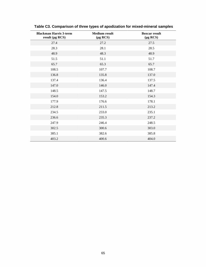
65
Table C3. Comparison of three types of apodization for mixed-mineral samples
Blackman Harris 3-term
result (µg RCS)
Medium result
(µg RCS)
Boxcar result
(µg RCS)
27.4 27.2 27.5
28.3 28.1 28.5
48.9 48.3 48.9
51.5 51.1 51.7
65.7 65.3 65.7
108.5 107.7 108.7
136.8 135.8 137.0
137.4 136.4 137.5
147.0 146.0 147.4
148.5 147.5 148.7
154.0 153.2 154.3
177.9 176.6 178.1
212.8 211.5 213.2
234.5 233.0 235.1
236.6 235.3 237.2
247.9 246.4 248.5
302.5 300.6 303.0
385.1 382.6 385.8
403.2 400.6 404.0
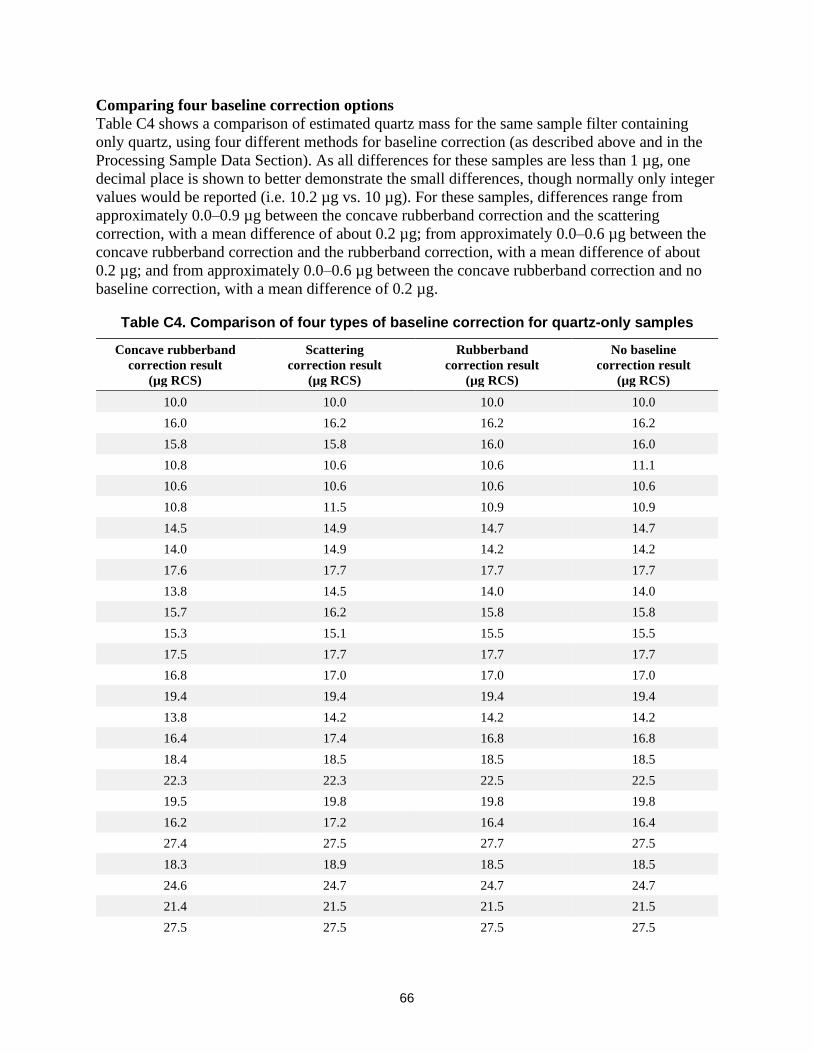
66
Comparing four baseline correction options
Table C4 shows a comparison of estimated quartz mass for the same sample filter containing
only quartz, using four different methods for baseline correction (as described above and in the
Processing Sample Data Section). As all differences for these samples are less than 1 µg, one
decimal place is shown to better demonstrate the small differences, though normally only integer
values would be reported (i.e. 10.2 µg vs. 10 µg). For these samples, differences range from
approximately 0.0–0.9 µg between the concave rubberband correction and the scattering
correction, with a mean difference of about 0.2 µg; from approximately 0.0–0.6 µg between the
concave rubberband correction and the rubberband correction, with a mean difference of about
0.2 µg; and from approximately 0.0–0.6 µg between the concave rubberband correction and no
baseline correction, with a mean difference of 0.2 µg.
Table C4. Comparison of four types of baseline correction for quartz-only samples
Concave rubberband
correction result
(µg RCS)
Scattering
correction result
(µg RCS)
Rubberband
correction result
(µg RCS)
No baseline
correction result
(µg RCS)
10.0 10.0 10.0 10.0
16.0 16.2 16.2 16.2
15.8 15.8 16.0 16.0
10.8 10.6 10.6 11.1
10.6 10.6 10.6 10.6
10.8 11.5 10.9 10.9
14.5 14.9 14.7 14.7
14.0 14.9 14.2 14.2
17.6 17.7 17.7 17.7
13.8 14.5 14.0 14.0
15.7 16.2 15.8 15.8
15.3 15.1 15.5 15.5
17.5 17.7 17.7 17.7
16.8 17.0 17.0 17.0
19.4 19.4 19.4 19.4
13.8 14.2 14.2 14.2
16.4 17.4 16.8 16.8
18.4 18.5 18.5 18.5
22.3 22.3 22.5 22.5
19.5 19.8 19.8 19.8
16.2 17.2 16.4 16.4
27.4 27.5 27.7 27.5
18.3 18.9 18.5 18.5
24.6 24.7 24.7 24.7
21.4 21.5 21.5 21.5
27.5 27.5 27.5 27.5
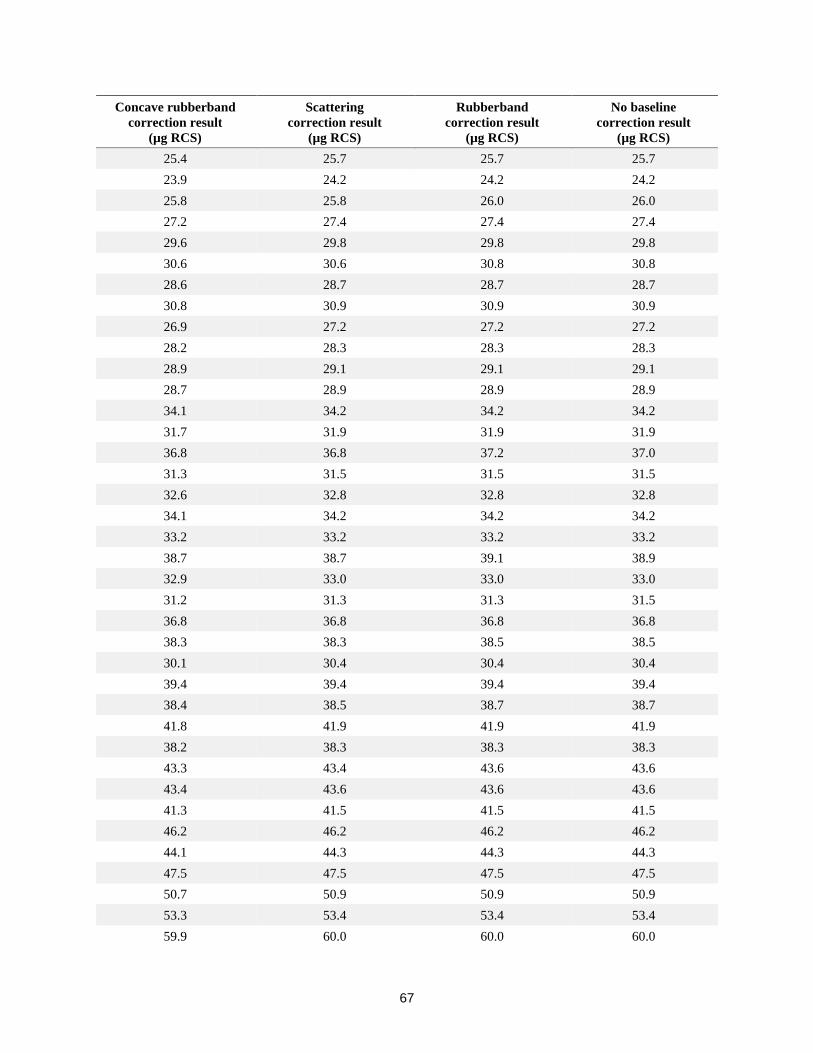
67
Concave rubberband
correction result
(µg RCS)
Scattering
correction result
(µg RCS)
Rubberband
correction result
(µg RCS)
No baseline
correction result
(µg RCS)
25.4 25.7 25.7 25.7
23.9 24.2 24.2 24.2
25.8 25.8 26.0 26.0
27.2 27.4 27.4 27.4
29.6 29.8 29.8 29.8
30.6 30.6 30.8 30.8
28.6 28.7 28.7 28.7
30.8 30.9 30.9 30.9
26.9 27.2 27.2 27.2
28.2 28.3 28.3 28.3
28.9 29.1 29.1 29.1
28.7 28.9 28.9 28.9
34.1 34.2 34.2 34.2
31.7 31.9 31.9 31.9
36.8 36.8 37.2 37.0
31.3 31.5 31.5 31.5
32.6 32.8 32.8 32.8
34.1 34.2 34.2 34.2
33.2 33.2 33.2 33.2
38.7 38.7 39.1 38.9
32.9 33.0 33.0 33.0
31.2 31.3 31.3 31.5
36.8 36.8 36.8 36.8
38.3 38.3 38.5 38.5
30.1 30.4 30.4 30.4
39.4 39.4 39.4 39.4
38.4 38.5 38.7 38.7
41.8 41.9 41.9 41.9
38.2 38.3 38.3 38.3
43.3 43.4 43.6 43.6
43.4 43.6 43.6 43.6
41.3 41.5 41.5 41.5
46.2 46.2 46.2 46.2
44.1 44.3 44.3 44.3
47.5 47.5 47.5 47.5
50.7 50.9 50.9 50.9
53.3 53.4 53.4 53.4
59.9 60.0 60.0 60.0
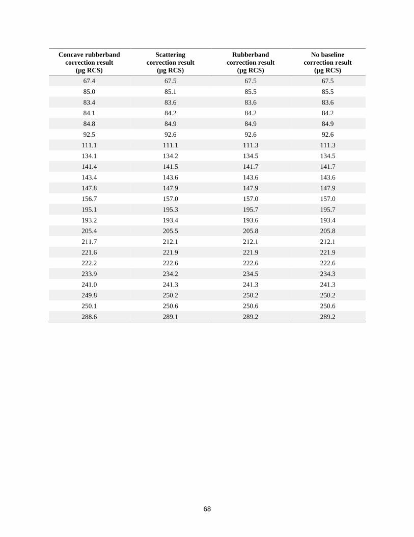
68
Concave rubberband
correction result
(µg RCS)
Scattering
correction result
(µg RCS)
Rubberband
correction result
(µg RCS)
No baseline
correction result
(µg RCS)
67.4 67.5 67.5 67.5
85.0 85.1 85.5 85.5
83.4 83.6 83.6 83.6
84.1 84.2 84.2 84.2
84.8 84.9 84.9 84.9
92.5 92.6 92.6 92.6
111.1 111.1 111.3 111.3
134.1 134.2 134.5 134.5
141.4 141.5 141.7 141.7
143.4 143.6 143.6 143.6
147.8 147.9 147.9 147.9
156.7 157.0 157.0 157.0
195.1 195.3 195.7 195.7
193.2 193.4 193.6 193.4
205.4 205.5 205.8 205.8
211.7 212.1 212.1 212.1
221.6 221.9 221.9 221.9
222.2 222.6 222.6 222.6
233.9 234.2 234.5 234.3
241.0 241.3 241.3 241.3
249.8 250.2 250.2 250.2
250.1 250.6 250.6 250.6
288.6 289.1 289.2 289.2
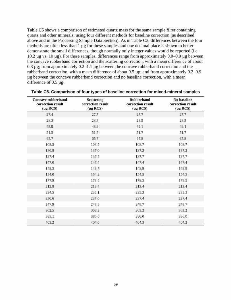
69
Table C5 shows a comparison of estimated quartz mass for the same sample filter containing
quartz and other minerals, using four different methods for baseline correction (as described
above and in the Processing Sample Data Section). As in Table C3, differences between the four
methods are often less than 1 µg for these samples and one decimal place is shown to better
demonstrate the small differences, though normally only integer values would be reported (i.e.
10.2 µg vs. 10 µg). For these samples, differences range from approximately 0.0–0.9 µg between
the concave rubberband correction and the scattering correction, with a mean difference of about
0.3 µg; from approximately 0.2–1.1 µg between the concave rubberband correction and the
rubberband correction, with a mean difference of about 0.5 µg; and from approximately 0.2–0.9
µg between the concave rubberband correction and no baseline correction, with a mean
difference of 0.5 µg.
Table C5. Comparison of four types of baseline correction for mixed-mineral samples
Concave rubberband
correction result
(µg RCS)
Scattering
correction result
(µg RCS)
Rubberband
correction result
(µg RCS)
No baseline
correction result
(µg RCS)
27.4 27.5 27.7 27.7
28.3 28.3 28.5 28.5
48.9 48.9 49.1 49.1
51.5 51.5 51.7 51.7
65.7 65.7 65.8 65.8
108.5 108.5 108.7 108.7
136.8 137.0 137.2 137.2
137.4 137.5 137.7 137.7
147.0 147.4 147.4 147.4
148.5 148.7 148.9 148.9
154.0 154.2 154.5 154.5
177.9 178.5 178.5 178.5
212.8 213.4 213.4 213.4
234.5 235.1 235.3 235.3
236.6 237.0 237.4 237.4
247.9 248.5 248.7 248.7
302.5 303.2 303.2 303.2
385.1 386.0 386.0 386.0
403.2 404.0 404.3 404.2
Promoting productive workplaces through safety and health research DHHS (NIOSH) Publication No. 2022-108DOI: https://doi.org/10.26616/NIOSHPUB2022108