Digital Comprehensive Summaries of Uppsala Dissertationsfrom the Faculty of Science and Technology 34

Understanding Ionic Conductivity in Crystalline Polymer Electrolytes

DANIEL BRANDELL

ISSN 1651-6214ISBN 91-554-6204-9urn:nbn:se:uu:diva-5734

ACTAUNIVERSITATIS

UPSALIENSISUPPSALA

2005

List of Papers

This thesis is a summary based on the following papers, which are referred to in the text by their Roman numerals I-IV.

I. Molecular dynamics simulation of the LiPF6 PEO6 structure D. Brandell, A. Liivat, H. Kasemägi, A. Aabloo and J.O. Thomas J. Mater. Chem., 15 (2005) DOI:10.1039/b417232a.

II. Conduction mechanisms in crystalline LiPF6 PEO6 doped with SiF6

2-- and SF6D. Brandell, A. Liivat, A. Aabloo and J.O. Thomas

Submitted to Chemistry of Materials.

III. Molecular dynamics simulations of the crystalline short-chain polymer system LiPF6 PEO6 (Mw~1000)

D. Brandell, A. Liivat, A. Aabloo and J.O. Thomas Submitted to Journal of Materials Chemistry.

IV. A molecular dynamics study of ion conduction mechanisms in crystalline low-Mw LiPF6 PEO6

D. Brandell, A. Liivat, A. Aabloo and J.O. Thomas In manuscript.

Comment on my contribution to this work: I-IV: Project planning; MD calculations and the majority of the analyses; preparation of all the manuscripts.

Other published papers not included in this thesis:

Calculations of the optical absorption spectrum of ErCl3 in poly(ethylene oxide) (PEO) D. Brandell, M. Klintenberg, A. Aabloo and J.O. Thomas International Journal of Quantum Chemistry, 80 (2000) 799.

The effect of polymer host on optical absorption spectra for Er(CF3SO3)3 in poly(ethylene oxide)n for n = 100 to 25 D. Brandell, M. Klintenberg, A. Aabloo and J.O. Thomas Journal of Materials Chemistry, 12 (2002) 565.

Optical absorption spectra from rare-earth ions in polymers: the effect of the polymer hostD. Brandell, M. Klintenberg, A. Aabloo and J.O. Thomas Macromolecular Symposia, 186 (2002) 51.

Contents

1. Introduction.................................................................................................9 1.1 Energy sources and energy storage ......................................................9 1.2 The Li-ion polymer battery ..................................................................9 1.3 Understanding conductivity ...............................................................10

2. Polymer electrolytes..................................................................................12 2.1 General concepts ................................................................................12

2.1.1 A definition.................................................................................12 2.1.2 Thermodynamics ........................................................................13 2.1.3 Polymers, salts and modifiers .....................................................14 2.1.4 Conductivity mechanism ............................................................15

2.2 Crystalline polymer electrolytes.........................................................16 2.3.1 Implications of the structures......................................................19

2.3 LiXF6 PEO6 ........................................................................................20 2.4 Molecular Dynamics studies of LiPF6 PEO6......................................21

3. Molecular Dynamics.................................................................................23 3.1 Computational Chemistry ..................................................................23 3.2 The simulation method.......................................................................24

3.2.1 Interaction potentials ..................................................................25 3.2.2 Periodic boundary conditions and other requirements................27 3.2.4 Non-equilibrium MD..................................................................28

3.3 Structure and dynamics from MD simulations...................................29 3.3.1 Radial distribution functions.......................................................29 3.3.2 Bond- and dihedral-angle plots...................................................30 3.3.3 Folding and thermal displacement parameters ...........................30 3.3.4 Diffusion and conductivity .........................................................31 3.3.5 Time-correlation studies .............................................................32

3.4 MD vs. experiment .............................................................................32

4. Structure....................................................................................................34 4.1 Coordination.......................................................................................34 4.2 Polymer configuration........................................................................36 4.3 Chain-end effects................................................................................37 4.4 Local effects of doping.......................................................................38 4.5 Structural effects of an applied electric field......................................39

4.6 Macroscopic nature of the material ....................................................41 4.7 Calculated diffraction profiles............................................................43

5. Dynamics ..................................................................................................45 5.1 Thermal motion and displacement parameters...................................45 5.2 Ion hopping and conductivity.............................................................46 5.3 Mechanisms........................................................................................48 5.4 The effects of doping..........................................................................51 5.5 Long-chain vs. short-chain effects......................................................51

6. Concluding remarks – MD vs. experiment ...............................................53

Acknowledgements.......................................................................................55

Populärvetenskaplig sammanfattning ...........................................................56 Att förstå jonledning i kristallina polymerelektrolyter ........................56

References.....................................................................................................60

Abbreviations

CN Coordination Number CNF Coordination Number Function DFT Density Functional Theory EO Ether Oxygen LDA Local Density Approximation LIPB Lithium-Ion Polymer Battery MC Monte Carlo MD Molecular Dynamics MM Molecular Mechanics MSD Mean-Square Displacement MW Molecular Weight NEMD Non-Equilibrium Molecular Dynamics NMR Nuclear Magnetic Resonance PEG Poly(ethylene glycol) PEM Proton Exchange Membrane PEMFC Proton Exchange Membrane Fuel Cell PEO Poly(ethylene oxide) PPO Poly(propylene oxide) QM Quantum Mechanics RDF Radial Distribution Function VTF Vogel-Tamman-Fulcher

9

1. Introduction

1.1 Energy sources and energy storage The forthcoming energy crisis of the modern World raises fundamental questions to solve in the field of Science, as well as in the field of Politics. The World’s dominant energy sources today are fossil fuels – oil, coal and gas. These have well-known drawbacks; not least the contribution to the environmental problems of global warming through “the greenhouse effect”. Oil, which represents the greater part of the fossil fuels used today (40% of the World’s energy needs, and as much as 90% of its transport fuel), is – at least when it comes to what is economically justifiable to exploit – going to run out within the next few generations, and most of the unexplored re-sources are in politically unstable areas of the World. Eventually all fossil fuels will run out [1,2].

It is therefore understandable that researchers in many fields try to de-velop alternative energy sources. For example, in Sweden today there is an extensive use of water power, and additional energy can be generated from wind and waves, or from renewable bio-materials. However, these sources are far from sufficient to replace the energy we get today from fossil fuels, and to explore them further often means interfering with the environment. Instead, the main focus of the research community today is on developing solar cells and hydrogen-based fuel cells [3,4].

Within the framework of finding and using alternative energy sources, one is often faced with the problem of energy storage. One of the most con-venient techniques is electrochemical storage. The work presented in this thesis is ultimately conducted in the context of chemical storage in form of the Lithium-Ion Polymer Battery (LIPB).

1.2 The Li-ion polymer battery The main advantage of the LIPB is that it combines a high energy density, a high cell voltage and rechargeability. This means that the energy is stored effectively, that the battery can be used in many applications and that it can

10

be used over and over again. Besides, the batteries are comparatively reliable and safe [5,6].

The battery generally comprises an anode consisting of a lithium interca-lated graphite with a low electrochemical potential and a transition-metal oxide cathode with high potential (e.g., LiCoO2 or Li(CoNi)O2), which both can reversibly intercalate and release lithium ions [7]. Between the anode and cathode there is a polymer electrolyte separator – the focus in this thesis. Under discharge, the electrons travel from the anode to cathode. At the same time, Li+ ions are extracted from the anode, pass through the electrolyte, and into to the cathode. The task for the electrolyte is merely to facilitate this lithium transport – not as trivial as it may appear.

Figure 1. A schematic representation of the Lithium-Ion Polymer Battery (LIPB).

1.3 Understanding conductivity Polymers, like other solid materials, can experience two types of conductiv-ity: electronic (whose explorers were awarded the Nobel Prize in Chemistry in 2000 [8]) and ionic. The higher ionic conductivity, the more the charge that can be transported through an electrolyte per unit time.

11

For the Lithium-Ion Polymer Battery, the most suitable solid electrolytes are formed by mixing a lithium salt, typically LiPF6 or LiBF4, into poly(ethylene oxide) (PEO), -(CH2CH2O)n- [9,10]. However, these electro-lytes show satisfying ionic conductivity ( > 10-4 S. cm-1) only at tempera-tures above 70 C, where the polymer becomes amorphous. The conventional belief has been that the high degree of local order (“crystallinity”) is what makes the ionic conductivity too low at ambient temperatures. Therefore, much attention has been devoted to the task of increasing the amorphous content of the PEO electrolyte at ambient temperatures; either by using large-anion lithium salts [11,12], by adding liquid plasticizers [13,14] or ceramic fillers [15-17] to the polymer or by modifying the PEO with side-chains and cross-links [18-21].

The crystalline phases of the polymer electrolytes were for a long time re-garded as insulators. This view has been overturned during recent years by the demonstration of ionic conductivity in the complexes LiXF6 PEO6.(X = P, As or Sb) [22]. Although the conductivity was relatively low in these ma-terials, they still showed ten times higher ionic conductivity than their amor-phous counterparts. The LiXF6 PEO6 complexes also display very fascinat-ing structures [23,24] – the materials are composed of coaxial hemi-helices of PEO, which pairwise form cylindrical channels containing the lithium ions coordinated to ether-oxygen chains; the anions lie outside the hemi-helical pairs, with no direct contact to the lithium ions (see Fig. 2).

These facts raise new fundamental scientific questions to answer: how does ionic conductivity process take place in these materials? How is the ionic conductivity related to the structure of the material? And how can we improve it further? The Molecular Dynamics (MD) computer simulation technique can be of great help in answering these questions.

12

2. Polymer electrolytes

2.1 General concepts A polymer electrolyte consists of an inorganic salt dissolved in a polymer host. Conductive polymer-salt complexes were first described in the early 1970’s [25,26], and were quickly adopted by the electrochemical commu-nity, who recognized the potential of a flexible, plastic, ion transporting me-dium for vital applications such as energy storage and electrochemical dis-plays [27,28]. In contrast to the cases of brittle glassy or crystalline solid conductors, polymer materials can accommodate volume changes, which makes them particularly suited for applications together with intercalation materials, such as the anode and cathode in a rechargeable battery. And, in contrast to liquid electrolytes, polymer electrolytes do not leak any harmful chemicals, and are therefore much safer.

Unfortunately, the ionic conductivity of a polymer electrolyte is, at a given temperature, at least 100 or 1000 times less than in a liquid or the bet-ter ceramic electrolytes. But, although higher conductivity is preferable, its conductivity has been shown to be sufficient for applications in thin-film electrochemical cells. Today, polymer electrolytes are key components in Li-ion polymer batteries used in portable entertainment, computing and tele-communication equipment [29].

2.1.1 A definition A “polymer electrolyte” can refer to one of the following material types [9]:

A solvent-free polymer-salt system, where the ion conduction takes place in a phase formed by one or several dissolved salts in a high or low mo-lecular weight polar polymer matrix. This is the archetypal polymer elec-trolyte, and the one which will be considered in this thesis. A hybrid (gel) electrolyte, consisting of a semi-crystalline polymer net-work, whose amorphous regions are swollen with a polar liquid together with a dissolved salt. Here, the polymer merely serves to give good me-chanical stability, while the liquid electrolyte is contained in the capillar-ies of the host material.

13

A plasticized electrolyte, where small amounts of high dielectric constant solvent or nano-size particles have been added to a conducting polymer-salt system to increase its conductivity. An ionic rubber, which is essentially a low-temperature (“low” here is nevertheless above room temperature) molten salt mixture (like chloro-aluminates), rubberized by the addition of polymers into a three-dimensional network. Proton-exchange membranes (PEM.) used in particular in different types of solid polymer-electrolyte fuel cells (PEMFC). These membranes usu-ally have a high water content, and most often consist of a fluorocarbon polymer backbone with attached sulfonic acid groups. These sulfonic groups then mediate the transport of H3O+ through the membrane. Per-haps the most important example of this kind of polymer electrolyte is Nafion [30].

2.1.2 Thermodynamics When a salt is dissolved into a polymer matrix, the free energy change is given by the standard Gibbs free energy expression:

mixingmixingmixing STHG 2.1

Here, for Gmixing < 0, the mixing process occurs spontaneously. It is clear that one must consider changes in both entropy and enthalpy.

The enthalpy change, S, is most straightforward, consisting of a positive part from the lattice energy of the salt, and a negative part from ionic coordi-nation to the polymer. For a complete mixing, the ions should therefore not bind too efficiently to one other, but form bonds with the polymer solvent. For most polymer electrolytes, this means that cations should coordinate electrostatically to the polymer backbone, while the anions should diffuse freely in the matrix, with a minimum of interaction with the polymer and especially with the cations. A salt with a small univalent cation and a large anion seems to fulfil these requirements: low lattice enthalpy, weak ion-ion bonding and strong cation-polymer coordination [31].

The entropy change is more complex. First, there is a positive entropy contribution from the break-up of the crystal lattice of the ionic salt, and the subsequent disordering of the ions in the system. This effect is compensated for by an increased rigidity in the polymeric system when the cations cross-link different parts of the polymer, thereby reducing its translational and rotational motion. On the other hand, salt dissolution facilitates more poly-mer configurations via multidentate coordination to the cation – an effect which leads to an increase in entropy. Nevertheless, if S is negative, Gibbs free energy should become positive at higher temperatures, where out-

14

salting will occur – the very opposite effect of dissolution in most liquid systems [32].

2.1.3 Polymers, salts and modifiers As is evident from the discussion on the enthalpy of mixing, it is necessary that the polymer in a polymer electrolyte has a strong coordination to the cations. Therefore, polymers with groups or atoms that can serve as electron donors are most suitable. Such polymers can be found among the polyethers, polyimides or polythiols [33]. The most common polymer type used in polymer electrolytes has so far been PEO [34], and it is also the subject of investigation in this thesis. PEO shows sufficient thermal and chemical sta-bility, and has a spacing between the oxygen groups which is ideal for cation solvation (for example, both -(CH2CH2CH2O)n- and -(CH2O)n- are much poorer solvents [35]). Since PEO has no double bonds, it displays a large flexibility and can therefore coordinate to many different types of cation.

In many applications though, the aim is to limit the crystallinity of the system. In battery applications, for example, ion conduction has been shown to take place in the amorphous phase. The disadvantage of PEO as a salt host then becomes apparent, since ~70-95% of pure PEO is crystalline at room temperature, depending on its molecular weight [36]. Therefore, much re-search effort has been invested in modifying the polymer to prevent it from crystallizing, e.g., by attaching a methyl group to the monomer unit to create poly(propylene oxide), PPO [37]. However, PPO and other modified sys-tems are much less able to dissolve salts than PEO. Better results have been achieved with block copolymers, comb-polymers or cross-links – all are ways to prevent PEO from crystallizing [38].

Other ways to increase the “amorphicity” of the systems have been to in-troduce small additives, plasticizers or nano-size particles into the polymer host. They disturb the local crystal field and suppress order [39]. These addi-tives have been shown to increase the conductivity with several orders of magnitude. The presence of a plasticizer like poly(ethylene glycol), PEG, also results in a lower glass transition temperature, Tg, due to weaker interac-tions between the ions and the polymer chain, and can furthermore cause higher ion dissociation [40].

The ether oxygens in PEO are hard Lewis bases, i.e., they have low po-larizability and high electronegativity. They thus coordinate well to hard Lewis acids, which in general are small cations with no valence electrons, e.g., Li+, Na+, Mg2+ and Ca2+. These cations then, in turn, form salts with low lattice energies together with large, polyatomic anions with high polarizabil-ity, e.g., BF4

-, PF6-, AsF6

-, ClO4-, SCN-, CF3SO3

- (triflate), (CF3SO3)2N-

(TFSI) or BPh4-. These larger anions can sometimes also have a plasticizing

effect on the polymer [41].

15

2.1.4 Conductivity mechanism The ion conductivity ( ) of a dilute homogeneous system at temperature T can generally be expressed as:

iiii uqnT )( 2.2

where ni is the number of charge carriers of type i, qi their charge and ui their mobility. Since the mobility in the same type of system is related to the dif-fusion coefficient (D) according to the Einstein relation, the molar conduc-tivity ( m) can be related to the diffusion by the Nernst-Einstein equation:

)( 222

DzvDzvRTF

m 2.3

Here, + and - are the number of positive and negative ions per formula unit and z+ and z- their respective charges, while F is Faraday’s constant.

Ion conductivity is usually measured experimentally by impedance spec-troscopy, while the diffusion coefficient can be estimated from MD simula-tions – there therefore exists a direct link between calculation and experi-ment regarding the dynamics in these systems.

In the early 1980’s, Berthier et al. [42] were the first to show from NMR studies that the predominant conduction in a PEO-based electrolyte was tak-ing place in the amorphous phase. This led Ratner et al. [43] to propose a mechanism for long-range cation transport, the dynamic bond percolation theory, where ionic transport is closely connected to the flexibility of the polymer backbone. About the same time, the variation of with temperature for a fully amorphous polymer electrolyte was shown to be more accurately expressed by the Vogel-Tamman-Fulcher, VTF, Eq. 2.4, rather than by the normal Arrhenius expression:

)(exp

00 TTR

EA 2.4

where EA the activation energy, and 0 the conductivity at a reference tem-perature T0. The VTF behaviour can describe the diffusion of uncharged molecules through disordered media such as fluids or polymers. Within dy-namic bond percolation theory, this is modified to describe cation transport by the semi-random motion of local polymer segments, and the activation energy in Eq. 2.4 can be related to rotational barriers in the polymer chain [44]. This motion will create new coordination sites for the cations, while the old sites disappear. The ions jump from site to site, either along the same

16

chain or between chains; this process is mainly dependent on the structure of the local surroundings. The cations should not be attached too strongly to the ether oxygens. This is consistent with the observation that Mg2+ moves less easily than Li+ in high molecular weight systems [45].

Dynamic bond percolation theory has been further developed to take ion-ion interaction and anionic motion into account [46]. The anions, whose interaction with the polymer solvent have been shown to be weak, diffuse freely around in the matrix in the free space created by the polymer back-bone motion. This leads generally to a high transference number t- for the anions, which is a drawback in cation intercalation materials. A high trans-ference number t+ for the cations would mean a more efficient electrolyte [47].

To optimize the performance of a polymer electrolyte is complex. Me-chanical stability, solubility, ion-pairing, polymer flexibility, conductivity and transference numbers often vary in ways which make the overall result of a modification difficult to predict. In fact, recent research has seen little increase in the conductivity of polymer electrolytes, irrespective of the cho-sen route. A better understanding of the structural aspects governing conduc-tivity in polymer electrolytes could then lead the way to higher conductivi-ties [48]. It has also been shown that the main structural features of polymer electrolytes in their crystalline phases retained in their amorphous forms [49].

2.2 Crystalline polymer electrolytes Crystalline PEO-salt complexes form only a few discrete compositions, usu-ally at a comparatively high salt concentration, e.g., 1:1 or 1:3. It has shown to be nigh on impossible to grow high quality crystals of polymer electro-lytes, so that powder diffraction has been the only realistic experimental tool. Although powder diffraction data provide considerably less information than single crystal data, ab initio structure determination techniques for powder data have been developed in recent years. Not least, the Monte-Carlo-based method of simulated annealing [50] has resulted in several new structure determinations.

A remarkably early report on a PEO-salt structure was HgCl2 PEO4 [51], although this should be seen rather as PEO containing HgCl2 molecules than a salt dissolved in a polymer matrix. The first reported crystal structure of a polymer electrolyte was thus for KSCN PEO4 [52] in 1983, but the structure was later shown to be incorrect [53]. Some years later, Chatani et al. pub-lished structures of NaI PEO3, NaSCN PEO3 and NaSCN PEO [54,55]. Thereafter, Bruce et al. have dominated the field, reporting crystal structures of compositions with cation: EO ratios 1:1, 1:3, 1:4, 1:6 and 1:8.

17

Figure 2. The LiPF6 PEO6 structure viewed along the chain axis.

In the highest concentrations (1:1), other known structures besides NaSCN PEO are NaCF3SO3 PEO [56] and KCF3SO3 PEO [57]. At such a high concentration, the cation-EO coordination number is as low as 2; in-stead, the cations coordinate to 4 anions. The two coordinated oxygens are located on the same polymer chain; the cations therefore do not cross-link the chains, nor do the ether oxygens. On the other hand, both SCN- and CF3SO3

- anions coordinate to cations associated with different chains and thus serve as cross-linkers. This leads to high melting points for these mate-rials. The polymer chain conformation in turn adopts a stretched zig-zag arrangement ggtggt with all C-C dihedral angles g or g and the C-O angles either t, g or g (the dihedral angles have throughout been defined as cis (c) in the range 0 45 ; trans (t) in the range 180 45 ; and the remainder as either gauche (g) or anti-gauche ( g )). Unlike other polymer-salt complexes, this zig-zag polymer conformation is unable to envelope the cations.

Compared to the 1:1 systems, there have been more studies of the more dilute 1:3 concentrations: NaI PEO3 [54], NaSCN PEO3 [55] NaClO4 PEO3[58], LiCF3SO3 PEO3 [59], LiN(CF3SO3)2 PEO3 [60,50], LiBF4 PEO3 [61] and LiAsF6 PEO3 [62] are all now crystal structure determined. In the 1:3 case, PEO adopts a helical conformation with all C-O dihedral angle transand the C-C bonds either gauche or anti-gauche. The repeat sequence is

18

gttgttgtt for all systems except LiAsF6 PEO3 and LiBF4 PEO3, where it is gttgttgtt . Na+ coordinates to 3 or 4 ether oxygens and 2 anions, while Li+

coordinates in all compounds to 3 oxygens and 2 anions. The anions bridge adjacent cations along the same polymer chain; i.e., there are no interchain links in these systems. The structure is thus only held together by weak van der Waals interactions. The cations are located inside the polymer helices.

Cations larger than Na+ demand a higher coordination number, which changes the structure of the polymer somewhat. This also means that the concentration of the stable compositions increase to 1:4. For this case, as well as for 1:3 compositions, there are several structures determined: HgCl2 PEO4 [51] KSCN PEO4 [53], NH4SCN PEO4 [53], RbSCN PEO4 [63] and ZnCl2 PEO4 [64]. The structures with divalent cations (HgCl2 PEO4 and ZnCl2 PEO4) are completely different from any known polymer electrolyte containing monovalent cations – the polymers form extended planes with the cations. The cations are here each coordinated to only two ether oxygens, leaving several oxygens uncoordinated.

The 1:4 structures with monovalent cations more resemble the 1:3 case. The cations are located within polymer helices, each coordinating to 5 ether oxygens and two anions; again the anions do not bridge between adjacent polymer chains. The polymer chain configuration involves four monomer units in their repeat sequence, forming a gttgttgttgtt sequence.

Further dilution result in the cation:EO composition 1:6. So far, only structures with polyatomic hexagonal anions and lithium cations – Li-AsF6 PEO6 [23], LiSbF6 PEO6 and LiPF6 PEO6, [24] – have been properly determined, although it is claimed that LiClO4 PEO6 [65] is iso-structural. This change in composition has a profound influence on the crystal structure, which can be seen in Fig 2. The cations and anions are now completely sepa-rated, which suggests that the anions (as in the amorphous phase) move freely without any well-defined coordination. The lithium cations each coor-dinate to five oxygens, three from one PEO chain and two from another. The polymer forms hemi-helices (“half-cylinders”) which pairwise forms chan-nels for the Li+ ions. The asymmetric unit contains six EO units and, al-though the overall hemi-helical structure is retained when substituting anion, the dihedral-angle conformation changes somewhat. The situation is com-plex, e.g., in LiPF6 PEO6, it is ctcggggttggttgctgt , and thus has several highly energetic cis-conformations.

Only one structure of the even more diluted 1:8 composition have been determined: NaBPh4 PEO8 [66]. As for the 1:3 and 1:4 concentrations, the polymer again forms a single-chain helical arrangement, but with planar rings consisting of five EO units around the Na+ ion. These rings are then each connected via three EO units. The Na+ ions have the coordination num-ber 7. The large BPh4

- ions lie between the helices, and do not coordinate to the cations.

19

2.3.1 Implications of the structures The structures of crystalline polymer electrolytes are summarized in Table 1. It is clear that lower concentration leads to less anionic and more Oet coordi-nation for the cations, while the polymer repeat unit becomes longer and more complex. Interestingly, the PEO conformation does not seem to be dependent on cation size. Inter-helical bridging only occurs for the very high concentration systems (1:1). This is also the only concentration where ca-tions are not located within helical or cylindrical PEO conformations. Not surprisingly, larger cations have higher coordination numbers, and the coor-dination number for different types of cation seems to be independent of concentration.

Table 1. Crystalline polymer electrolytes structures.

Conc. Cation coordination (Oet + anion) Polymer conformation Inter-helical

bridging

1:1 Na+, K+: 2 + 4 ggtggt Yes

1:3 Na+: (3,4) + 2 Li+: 3 + 2

gttgttgtt orgttgttgtt No

1:4 K+, NH4+, Rb+: 5 + 2 gttgttgttgtt No

1:6 Li+: 5 + 0 ctcggggttggttgctgt No 1:8 Na+: 7 + 0 gggtctggtgggttgtggtggtgg No

It has been suggested that the helical form of PEO, with the cations inside the chain, is retained above the glass transition temperature [67]. This is also consistent with the relatively low melting temperature of these materials (except for 1:1 concentrations); if only the van der Waals bonds between the polymer chains are broken during melting, the process does not demand much energy.

It is tempting to assume that the cations move along and within the heli-ces, which would make ionic transfer between the different helices the rate-determining step. It follows, that local order and orientation of the helices should facilitate the conduction process. There is also experimental evidence to support this: stretching a polymer electrolyte, and thus creating local order in the form of chain alignment, can enhance conductivity [68], as can the ordered arrangement of PEO in hydrophobic blocks [69].

Anisotropic systems call for different theoretical concepts and mathemati-cal descriptions of the ionic conductivity than those used for amorphous systems. Furthermore, extreme cases of molecular anisotropy can give mesophases which display both solid- and liquid-phase properties. Such phases are also known as liquid crystals, with long-range order in two direc-tions and liquid-like disorder in the third – reminiscent of the structures of a highly concentrated polymer electrolytes above Tg. One type of such order

20

occurs in a smectic phase (from the Greek word for soapy; Fig. 3a), where the molecules align to form layers. Other liquid crystals lack this layered structure but retain parallel alignment; such mesophases are called nematic(from the Greek word for thread; Fig. 3b) [70].

Figure 3. Smectic (a) and nematic (b) mesophases.

Concentration is also relevant in this structural picture: in highly concen-trated systems (above 1:6), there exists extensive ion-pairing, which can be assumed to persist after melting. In less concentrated systems, no such ion-pairing is evident, and these systems tend to display higher conductivity. To develop polymer electrolytes with higher conductivity, we would appear to need structures with:

Low ion-pairing, i.e., relatively low concentration. High local order. Liquid-crystal like structures.

2.3 LiXF6 PEO6

Although the structure of crystalline polymer-salt complexes is a fascinating subject in itself and can give a deeper understanding of conduction in the amorphous phase, some of these materials – the LiXF6 PEO6 (X=P,As,Sb) family – have even more interesting properties. As mentioned in the Intro-duction, these compounds have been shown to have higher ionic conductivi-ties than their amorphous counterparts; ca. 10-8 S cm-1 compared to 10-9 S cm-1 at room temperature.

21

They are also known to have unusual structures, which are believed to be the reason for their enhanced conductivities. Although the conductivity val-ues are much lower than for highly conductive amorphous PEO salts like LiTFSI PEO6, it has been shown that the conductivity can be further in-creased by 1-2 orders of magnitude by replacing 5% by isovalent TFSI (higher doping leads to phase separation) [71]. Similar improvements are found for ca. 1% anionic substitution with aliovalent SiF6

2- [72]. NMR measurements have indicated that the cations are the more mobile

ion, and that their motion is decoupled from the polymer [22]. Hence, it has been suggested that Li+ ions alone are the charge carriers; i.e., t+ = 1. As mentioned earlier, this is ideal for Li+ intercalation applications. A mecha-nism has been proposed in which Li+ ions jump between 5-coordinated sites via an intermediate 4-coordinated meta-stable site [73]; this has not so far been experimentally established.

An interesting phenomenon in the materials have further been that the low molecular weight (~2000) PEO complex phases LiAsF6 PEO6 and LiSbF6 PEO6 show two distinct qualitatively different phases, while LiPF6 PEO6 does not [74]. The second -phase, whose structure has so far not been published, is believed to consist of PEO helices resembling those of NaBPh4 PEO8, with the Li+ ions each coordinating six ether oxygens [75] – the highest coordination number for lithium in any known polymer-salt structure. This -phase forms spontaneously after melting of -LiSbF6 PEO6. This phase-change phenomenon is not found for high molecu-lar weight PEO, which is a clear indication of structural sensitivity to poly-mer Mw.

Samples of LiSbF6 PEO6 with different polymer Mw have also been shown to have different conductivies – highest for the lowest PEO Mw val-ues [73]. This has so far been explained by the decrease in crystallite size which occur at higher PEO Mw, although this cannot explain the different activation energies in the systems.

The effect of different molecular weights must be explored further in the LiXF6 PEO6 system. Very low molecular weights (Mw ~500) have been used in many of the structure and conductivity studies. Yet, the methoxy end-groups have been neglected in the structure determinations, eventhough the concentration of this obvious “defect” is high. In structure determinations of other PEO-salt structures, this “end-group effect” has led to unrealistically short or long C-C and C-O bonds [66]. The rôle of the end-groups in deter-mining ion conductivity is still unknown, and will be probed here.

2.4 Molecular Dynamics studies of LiPF6 PEO6

The first Molecular Dynamics (MD) studies of LiPF6 PEO6 are presented in this thesis. MD is a computational technique for studying both structural and

22

dynamical properties of materials. The thesis work deal with the PF6- anion

(and not AsF6- or SbF6

-) since LiPF6 has so far been the most commonly exploited lithium salt in lithium-ion polymer battery applications [5]; albeit, not the most stable.

In paper I; the structure from MD simulation is compared with that de-termined by experimental diffraction techniques. The PEO chains are here approximated to be infinite; this system is thus referred to as the infinite model hereafter. In paper II; the dynamics – not least the conduction mechanism – of the infinite LiPF6 PEO6 model is studied via simulation of the system under imposed external electric fields. The effect of doping with SF6 and SiF6

2-

(charge compensated by either withdrawing or inserting a Li+ ion, respec-tively) is also studied. In paper III; the structure of a methoxy end-capped low molecular weight PEO system is studied; referred to as the short-chain model hereafter. This model better reflects the real material than the infinite PEO chain model studied in papers I and II. Both smectic and nematic sub-systems are simulated. In paper IV; the dynamics and the effects of doping the methoxy end-capped low Mw PEO system (of paper III) is again explored by imposing a range of electric fields on the system. As in paper II, the effect of alio-valent doping is also studied.

23

3. Molecular Dynamics

3.1 Computational Chemistry Since the development of the first computers in the early 1950’s, scientist have tried to explore how these machines might be used in Chemistry. From the very beginning, the field of Computational Chemistry focused either on solving complex mathematical problems, typically quantum mechanical, or has tried to model the dynamical behaviour of atomic and molecular sys-tems. The boundaries between these two areas have never been well defined and, today, we see a convergence between quantum chemistry and simula-tion in studying chemical reactions [76].

With advances in computer technology leading to ever faster computers, Computational Chemistry has become an increasingly reliable tool for inves-tigating systems where experimental techniques still provide too little infor-mation. Ultra-fast spectroscopy can be used to follow fast reactions but only at a molecular level. A variety of diffraction techniques can also give de-tailed information about crystalline structure, but have difficulties monitor-ing changes at a molecular level. This is why the exponential growth in computer power has led to a corresponding growth in the number of compu-tational chemists and in the variety of different computational techniques available for solving chemical problems: ab initio Quantum Mechanics (QM), semi-empirical methods, Density Functional Theory (DFT), Monte Carlo (MC), Molecular Mechanics (MM), Molecular Dynamics, QM/MM, Car-Parrinello, etc.

There are two main branches within the Computational Chemistry com-munity: the computationally expensive methods which try to explore the electronic structure of small systems or systems with fixed crystal structures by quantum mechanical methods; and methods which focus on the atomic structure and dynamics of much larger systems but using less complex calcu-lations. In this thesis, the focus is on the latter – simulating atomic and mo-lecular interaction with the mathematics of classical mechanics. The follow-ing text is based on [77-80].

24

3.2 The simulation method In reality, atoms and molecules in solid materials are far from static unless the temperature is low; but even at 0K, vibrational motion remains. For ioni-cally conductive materials, atomic movement is the subject of major interest. Molecular Dynamics allows us to simulate the dynamics of the particles in a well-defined system to gain greater insights into local structure and local dynamics – such as ion transport in solid materials.

In an MD simulation, atomic motion in a chemical system is described in classical mechanics terms by solving Newton’s equations of motion:

iii amF 3.1

for each atom i in a system of N atoms; mi is their respective atomic mass; ai= d2ri/dt2 is their acceleration; and Fi is the force acting upon atom i due to interactions with all other particles in the system. The forces are generated from a universal energy potential E:

2

2

dtrd

mFrddE i

iii

3.2

The basic idea of MD goes back to a classical idea in Physics – that if one knows the location of all the particles in the Universe, and the forces acting between them, one is able to predict the entire future. In a normal MD simu-lation, this Universe comprises only a few thousand atoms; in extreme cases, upto a million.

With Newton’s equations, it is possible to calculate sequentially the loca-tions and velocities of all particles in the system. This generates a sequence of snapshots which constitutes a “movie” of the simulated system on the atomic scale. Due to the massive computer time necessary to solve these equation for a large number of particles, the movies are generally fairly short – in this work in the pico- or nanosecond regime. All that is needed to solve the equations of motion are the masses of the particles and a description of the potentials, E.

The solution of this set of equations is managed by a computer algorithm – here the so-called “leapfrog”. It works stepwise by:

- Calculating the acceleration at time t according to Equation 3.2.

- Updating the velocity vi at t + t/2 using

ttattvttv iii )()2/()2/( 3.3

25

where t is the time-step between two snapshots; here 0.1-1.0 fs.

- Calculating the atom position in the snapshot using:

tttvtrttr iii )2/()()( 3.4

The MD simulation method is very straightforward, but one must bear in mind that it is based on some severe approximations. At the highest level, the Born-Oppenheimer approximation is made, separating the wavefunction for the electrons from those of the nuclei. The Schrödinger equation can then be solved for every fixed nuclear arrangement, giving the electronic energy contribution. Together with the nuclear-nuclear repulsion, this energy deter-mines the potential energy surface, E.

At the next level of approximation, all nuclei are treated as classical parti-cles moving on the potential energy surface, and the Schrödinger equation is replaced by Newton’s equations of motion.

At the lowest level of approximation, the potential energy surface is ap-proximated to an analytical potential energy function which give the poten-tial energy and interatomic forces as a function of atomic coordinates.

3.2.1 Interaction potentials Since the analytical description of the potential energy surface, the force field, strictly determines the outcome of any MD simulation, it is necessary that this description is as precise as possible. The common methodology is thus to generate specific potentials for the simulated system. These can be generated and fine-tuned in two different ways: empirically or non-empirically.

Empirical potentials are derived by fitting the potential expression to macroscopic experimental observables, such as bond length, lattice parame-ters, bond vibrations, density, pressure, temperature, etc. Such potentials thus reproduce the properties they are modelled on extremely well, but can fail when it comes to other properties. In the simulations in this thesis work, the intermolecular potentials for PEO have been fine-tuned to reproduce pres-sure, structure and density [81].

Non-empirical potentials are derived from high-level ab initio calcula-tions. The structural and thermodynamical properties of the system are thus not intrinsically dependent on any experimental quantities, which makes comparison with such data a good test for the validity of the model. Single-point energy calculations are used to map the potential energy surface, and the analytical expressions for the potentials are then fitted to reproduce the surface. To get a good picture of the energy surface, the analytical expres-

26

sion is usually for from calculations made on for several different geometries and local configurations. An example of this procedure for Li-SiF6

2- interac-tions can be seen in Fig. 4.

Figure 4. Development of potentials for Li+-SiF62--interactions.

In this thesis, where the main focus is on conduction mechanism, it is an advantage to use potentials which well reproduce interactions at an atomic and molecular level. Non-empirical potentials derived from quantum chem-istry has thus been used for most interactions. Intramolecular potentials for the PEO backbone or the polyatomic anions have been described by typical two-, three- or four-body interactions:

20

1 )(2

)( rrkrVbond 3.5

20

2 )(2

)( kVbend 3.6

6

0cos)1()(

n

nnntorsional aV 3.7

while the intermolecular potentials have been described by electrostatic and two-body interactions in either the Born-Mayer-Huggins form:

46/

0

21

4)(

rD

rCAe

rqqrV Br

HMB 3.8

or the Lennard-Jones form:

27

rqq

rC

rArV JL

0

21612 4

)( 3.9

where k1, r0, k2, 0, an, A, B, C and D are constants depending on the inter-acting atom-types involved. The sources of all potentials used are listed in Table 2.

Table 2. Sources of the potentials used in the simulations.Potential Source

Intra- and intermolecular potentials for PEO [81], [82] PEO methoxy end-groups [83], [84] LiPF6 intramolecular and interaction with PEO [85-87] SiF6

2- intramolecular and interactions with LiPF6 and PEO [88] SF6 intermolecular [89], paper II

The total force field acting on an atom i in the simulation is then the sum of interactions with all other particles in the box:

i i ji kiJLHMBtorsbend

ribond rVrVVVrVV

, , , ,,)()()()()(

3.2.2 Periodic boundary conditions and other requirements Since the computation time required to calculate the trajectories of all N particles in a simulation box increases with N2, the simulated system cannot be made large enough to accurately represent the bulk properties of an actual crystal or amorphous material: surface effects will always be present. This problem is solved by implementing periodic boundary conditions, in which the simulation box is replicated through space in all directions; see Fig 5. The set of atom present in the box is thus surrounded by exact replicas of itself, i.e. periodic images. If an atom moves though a boundary on one side of the simulation box, so will its replica on the other side. This keeps the number of atoms in one box constant, and if the box has constant volume the simulation then preserves the density of the system. The periodic boundary conditions introduce an artificial periodicity of the system, which can effect the properties of the simulation, but much less than the surface effect would have done without the periodicity.

28

Figure 5. Periodic boundary conditions in two dimensions.

An MD simulation should also follow the laws of thermodynamics. At equi-librium, it should have a specific temperature, volume, energy, density, pres-sure, heat capacity, etc. In statistical thermodynamics, this constitutes the state of the system; its ensemble. Since MD is a statistical mechanics method, an evaluation of these physical quantities can be made from the velocities and masses of the particles in the system, and MD can serve as a link between these atomic-level quantities and macroscopic properties. When performing an MD simulation, one chooses a specific ensemble in which the simulation model is retained. This ensemble then scales the ve-locities of the particles. Three different ensembles have been used here:

1. The microcanonical ensemble (NVE), which maintains the system under constant energy (E) and with constant number of particles (N) in a well-defined box with volume (V). This is appropriate during the initial equilibration phase of a simulation.

2. The isothermal-isobaric ensemble (NPT), where temperature and pres-sure are kept constant. This is normally the best model of the experimen-tal conditions, and was used for the calculations in paper I.

3. The canonical ensemble (NVT), where volume and temperature are kept constant. This ensemble has been used for most simulations in papers I,II, III and IV, so that comparisons can be made with experimental data from structures with fixed dimensions.

3.2.4 Non-equilibrium MD Chemical equilibrium is characterized thermodynamically in terms of uni-form pressure, temperature and chemical potentials. Non-equilibrium is characterized by gradients in these variables, leading to a flux in the system

29

which transports mass, momentum and charge along the gradient. This flux serves to destroy the gradient and bring the system to equilibrium. Non-equilibrium systems are thus characterized by mixing and dissipation proc-esses. Such processes arise in the discharge of a battery: electronic and ionic motion try to compensate for the difference in electrochemical potential be-tween cathode and anode. This gives rise to an electric field acting over the polymer electrolyte. The behaviour of crystalline LiPF6 PEO6 systems under such a field has been monitored in papers II and IV.

In non-equilibrium MD, a perturbation is switched on at time t = 0 and is held constant thereafter. The long-term steady-state response then yields transport coefficients. Problems occur though, since non-equilibrium sys-tems dissipate heat, leading to an increase in the temperature of the system. The field also gives rise to an undesirable material drift across the whole simulation box. These problems can be overcome by constantly re-scaling the velocities to maintain some desired temperature, and by fixing certain atoms to harmonic springs to hinder this drift. This has not been done here, however, since it is hard to justify the physicallity of this constraint. More-over, in a system where polymer-chain relaxation and ionic motion are criti-cal to the properties of interest, it is better to allow some drift in the system than to keep parts of it fixed.

Non-equilibrium raises some special concerns; he major problem is the choice of electric strength. It must be high enough to produce some measur-able response but not so high the drift becomes unrealistically large, leading to total destruction of the structure. This has proved a delicate balance. Moreover, high field values give rise to a non-linear response in different properties in the systems, e.g., the conductivity. This phenomenon has also been seen in other NEMD simulations [90]. This non-linearity means that it is difficult to compare properties calculated from these simulations with experiment.

3.3 Structure and dynamics from MD simulations The statistics provided by the MD simulations have been used to calculate different properties relating to structural and dynamical behaviour. This analysis and its chemical interpretation has been the major part of this thesis work.

3.3.1 Radial distribution functions One of the most important properties extracted from the MD simulation is the pair radial distribution function (RDF). It is a function, usually written ga...b(r), which presents the probability of finding a particle of type b at a distance r from particle of type a. In a perfect crystal without thermal mo-

30

tion, the RDF would appear as periodically sharp peaks, which gives infor-mation about the short-range order in the system.

The RDF can be calculated by counting the number of atom pairs within some distance range, and averaging this over a number of time-steps and particle pairs:

),()21(

),()( 1

rrVNM

rrNrg

ab

M

kabk

ab 3.11

where Nk is the number of atoms found at time k in a spherical shell of radius r and thickness r; and is the average system density, N/V, of a given atom type.

Integrating this RDF over r gives the coordination number function (CNF), which is the average coordination number of particle type a to parti-cle type b at distance r.

The RDF can be compared directly with experimental data from X-ray or neutron diffraction, and can thus be used as a check on the reliability of the potentials in many systems.

3.3.2 Bond- and dihedral-angle plots In a chemically complex system such as LiPF6 PEO6, average atomic dis-tances calculated as RDFs can be too rough a measurement to capture all the structural information available. The spatial arrangement of atoms can also be of major interest, and can be obtained throughout by calculating bond-angle and dihedral angle distributions in the crystallographic asymmetric unit. Since this involve 18 backbone carbons and oxygens in LiPF6 PEO6,and has 3 repeat units in the MD box, the angles have been plotted in a 3 6arrangement (see, for example, Fig. 4 in paper I). The total distribution of all 18 bond and dihedral-angles contains all the information we need on the polymer configuration.

Plotting especially the dihedral angles in this way gives space group in-formation for the simulated system, which can be related to the crystal-lographically determined space group. The appearance of new peaks indi-cates some new repeat unit

3.3.3 Folding and thermal displacement parameters Another way to study the simulated structure (paper I and III) and to com-pare it with experiment is to “fold” the atom positions back onto the crystal-lographic asymmetric unit (Fig. 6). This is done by applying the symmetry

31

operations of the space group for LiPF6 PEO6 (P21/a) in combination with translations. Doing this for several time-steps generates a distribution of atomic positions within the asymmetric unit, which can then be compared with crystallographic displacement parameters. The isotropic mean-square thermal displacement parameter (Uiso) for a given atom in the asymmetric unit is calculated from its mean-square displacements, 2, using:

N

kk rr

N 1

2,

2 1 3.12

for = x, y and z for atom position k. This gives:

)(31 222

zyxisoU 3.13

Figure 6. The operation of “folding” the content of the MD box back onto a crystal-lographic asymmetric unit.

3.3.4 Diffusion and conductivity The diffusion coefficient for an atom-type in a material can generally be calculated from an MD simulation via the time evolution of its displacement vector:

N

iiii zyx

NtD

1

222

61

3.13

32

From the diffusion coefficient, the conductivity can be calculated by the Nernst-Einstein equation (see Chapter 2). This is the most straightforward way of evaluating mobility in a simulated system. However, as argued in Section 3.2.4, the non-linearity in high-field systems make an absolute evaluation unrealistic. In these simulations (papers II and IV), diffusion and conductivity has therefore been treated in a comparative way by counting the number of ion-jumps for different field strengths in different systems.

3.3.5 Time-correlation studies Time correlation functions are perhaps the most convenient tool way to study dynamical properties. These relate some property B at a time t to some property A at t0:

0)()()( 00 tAB ttBtAtC 3.14

Here, A(t) and B(t) are dynamical variables of the system. If CAB grows to-wards unity, we have a maximum correlation between these properties. In this thesis, a correlation function has been used to monitor conduction mechanisms.

Correlation can also be calculated independent of time (i.e., at t = 0) – the straightforward probability that B occurs if A occurs can be readily measured from the MD statistics.

3.4 MD vs. experiment It has been argued that Computational Chemistry is both “theory” and “ex-periment”: “theory”, since clearly no measurements are made on a real sys-tem, and “experiment” since the potentials used are often based on experi-mental data on simple systems. MD is indeed often referred to as a “com-puter experiment”.

Today, most computational chemists would probably say that computa-tion is neither theory nor experiment, but rather a third leg on the chemical body – both to test theory and to interpret experiment; alternatively, to per-form “experiments” on systems inaccessible to normal experimental tech-niques.

This discussion puts focus on the relationship between MD and experi-ment. Experimentalists interpret their data using theories and models – they do not anticipate reality. Experimental data can often be interpreted in sev-eral ways, sometimes even within the same theoretical context. Not rarely are data interpreted on the basis of incorrect or inappropriate theory for the system under study. The interpretation of experimental results is not a search

33

for biblical “truth”, just like the computational chemist, the experimentalist uses models to make their interpretation, thereby creating a gap between themselves and reality. MD can indeed sometimes be as good (or bad) a method as experiment for modelling this reality.

34

4. Structure

The various MD simulations performed have provided a wealth of structuralinformation which is discussed here.

4.1 Coordination Starting from the infinite-chain system, CNFs and RDFs for Li-Li, Li-O and Li-P are plotted in Fig. 7. It can immediately be noted that there is some disagreement with some of the features of the experimentally determined structure; particularly, Li-O coordination is prevalently 6-fold, with a typical bond distance of 2.0 Å. In the experimental study, a Li coordination number of 5 was found, with three Oet’s from one PEO hemi-helical chain and two from the other, and with all bond distances in the range of 2.14-2.19 Å. The sixth oxygen was located more than 3 Å from the nearest lithium ion [24]. Interestingly, the MD-derived Li+ ion coordination corresponds closer to that found in the simulations of the equivalent short-chain polymer system (CH3(OCH2CH2OCH3)2 LiSbF6 [91].

It is also evident from the RDF that the Li+ ions inside the polymer chan-nels are equi-spaced at around 5.9 Å. This is also in conflict with the ex-perimental geometry, which involves two Li-Li distances (of 7.4 and 4.4 Å) along the chain. However, despite of these differences, the simulated infinite polymer-chain model is generally in agreement with the structure suggested from ND: the hemi-helical structure and the ion separation is retained.

When chain ends are introduced into the short-chain system, the coordina-tion changes; this is evident from Fig 7. The immediate impression is that the smectic and nematic models resemble one another more than they do the infinite-chain model; and also that the associated RDF peaks are much broader for both short-chain systems. This “liquid-like” peak broadening indicates greater structural relaxation in the short chain, where the Li-Li distances are also found to decrease somewhat compared to the infinite sys-tem.

The shortening of the polymer chain apparently also reduces the number of available coordination sites for Li+ ions: the Li+-Oet coordination de-creases to 5 instead of 6. This is also reflected in the CN of Oet to Li+: it is ca.0.8 at 3 Å for short chains, and 1.0 at the same distance in the infinite-chain system. This comparatively low CN is obviously the same as that suggested

35

0

1

2

3

4

3 4 5 6 7 8 9 10

r/Å

g Li...Li(r) infinite rdf

nematic rdf smectic rdf

(a)

0

5

10

15

20

25

0 1 2 3 4 5

r/Å

g Li...O(r)

infinite rdf infinite cnf nematic rdf nematic cnf smectic rdf smectic cnf

(b)

0

2

4

6

8

0 1 2 3 4 5 6 7 8

r/Å

g Li...P(r)

infinite rdf infinite cnf nematic rdf nematic cnf smectic rdf smectic cnf

(c)Figure 7. Radial distribution (RDF) and coordination number (CNF) functions for: (a) Li-Li, (b) Li-Oet and (c) Li-P. Note that curves for the smectic and nematic sys-tems almost totally overlap in (b) and (c).

from the neutron diffraction studies, but is here compensated for by an in-creased by Li+-PF6

- coordination (Fig. 7c). The CN (Li-P) value is ca. 0.5 at

36

4.0-5.0 Å in short-chain systems, implying that half the lithiums form ion-pairs or -clusters with the anions; a clear difference compared to the experi-mental and infinite-chain structures.

A small but perhaps significant difference appears between the smectic and nematic models in the form of a small peak at 3 Å in the Li-P RDF plot for the smectic system. This is found to correspond to extra Li+-PF6

- pairing in C2v and C3v configurations, bringing Li+ closer to the P atom of the anion; this is found to occur near the surface of the monodisperse smectic layers.

4.2 Polymer configuration On plotting the dihedral angles along the entire PEO backbone of the simula-tion box for the infinite-chain system, an obvious pattern emerges, suggest-ing the existence of an asymmetric unit of the same size as the experimen-tally determined structure (involving 6 EO units). That this same sequence length was found both from MD and from the diffraction studies must be seen as strong confirmation of the validity of the experimental crystallo-graphic space group (P21/a). Some discrepancies appear, however, between the simulated crystalline LiPF6 PEO6 system and the experimentally deter-mined structure. Firstly, the bond angles have a considerably smaller spread in the simulated system. Some extreme values in the experimental model, e.g., an -OCC- bond angle as low as 85 , lie far from the minimum in the bond-angle force field: the angular bond energy contribution drops from 217 kJ/mol to 16 kJ/mol during the simulation, implying that the experimentally determined structure may contain some unphysical details.

Fig 8. Dihedral-angle distribution in the infinite-chain system.

37

While agreement between simulated and experimental bond angles is was reasonably good, there is poorer correspondence between the distribution of the simulated dihedral angles and those found experimentally (see Fig. 8). While the experimental sequence of dihedral angles along the asymmetric unit is ctcggggttggttgctgt , the MD-derived sequence is

tcgcgtcttctgcgttct in the NPT simulation and tcggttctggggtgttct in the NVT simulation.

The MD-derived conformations more closely resemble those found in other crystalline PEO/salt complexes; cf., gttgttgtt for the crystal systems with EO:M+ ratios 3:1, and the gttgttgttgtt for EO:M+ ratios 4:1, where many low-energy trans-conformations for the -COCC- and -CCOC- dihedral angles predominate.

However, no repeat unit could be found in either of the short-chain mod-els (nematic and smectic),. Each dihedral angle is relatively stable, implying that the t/g/ g sequence is generally retained, although occasional shifts in some backbone units appear. Here, it is clear that the CCOC and COCC dihedral angles are generally t, while they are either g or g for the OCCO dihedral angles. This so-called “gauche effect” [92,93] for the OCCO dihe-dral angles is found in many crystalline and amorphous polymer systems, and is indeed implicit in the form of the backbone force-field model [81,82].

4.3 Chain-end effects In the short-chain systems, the chain-ends exhibit a broad variety of local conformations which are difficult to characterise systematically. Neverthe-less, some characteristics can be identified. It is evident (see, for example, Fig. 5 in paper III) that the distribution of chain-ends lies closer to the heli-cal axis in the nematic model, although no effective space-group is apparent. End-group displacements are also larger in the smectic system in the x-direction, as evidenced by the larger average end-to-end distance (45.05 Å compared to 43.97 Å).

One can also find different linkage and registry between chain end-groups. In several cases, terminal methyl groups on two adjacent short-chains within the same double-hemi helix (a situation which can only occur in the smectic model) tend to approach one another. The effective average distance between these neighbouring groups decreases somewhat during the simulation (from 5.02 to 4.80 Å), despite the fact that some of these dis-tances actually become much greater due to chain-end migration. The situa-tion is controlled by the Li+ ions close to the ends of the helices; when a Li+

ion remains close to and yet within the end of a helix, methoxy groups tend to wrap themselves around it, resulting in short distances between the methyl groups (see Fig. 9a). When a Li+ ion either leaves a helix and migrates into

38

the space between the smectic layers, or drifts in towards the centre of the helix, the chain-end pairs drift apart (Fig. 9b).

Fig 9.Different chain-end conformations in the smectic model of the short-chain system.

4.4 Local effects of doping Inserting a divalent SiF6

2- anion or a neutral SF6 molecule (with appropriate Li+ compensation) is seen to destabilize the local environment near the dopant. The more highly charged SiF6

2- anion also repels the neighbouring PF6

- ions; an effect which is compensated by the extraction of a Li+ ion from within the polymer hemi-helices, to form an Li+-SiF6

2- ion-pair with a net charge of –1. This occurs in all simulated infinite(LiPF6)0.99(Li2SiF6)0.01 PEO6 systems, and in most of the short-chain systems. This implies that, when Li+ is inserted far away from an SiF6

2- dopant, ion-pair formation creates a vacancy in an adjacent polymer helix.

Columns containing 5 or 7 Li+ ions differ slightly from those containing 6 Li+ ions; repulsion between the Li+ ions is obviously strong, forcing the Li+

ions into an equi-spaced arrangement. The Li-Li distance is ~6 Å for 6 Li+

ions within the helices; while a broader distribution extending to larger dis-tances is seen in the presence of a Li+ vacancy, as in the situation of SF6doping or when SiF6

2- extracts a Li+ ion from a helix. For helices with 7 Li+

ions, on the other hand, this Li-Li distance is shorter: 4.0 and 5.5 Å for the two types of site.

These changes in lithium distance also influence polymer geometry around the cations; the hemi-helical structure is always retained, but the di-hedral-angle conformation changes in most systems. The differences are relatively small, though, especially considering that the coordination num-bers and Li+-Li+ distances vary quite significantly. The equidistant spacing of the cations must cause relaxation of the polymer backbone, but the poly-

39

mer is evidently sufficiently rigidly to maintain its general conformation. The difference compared to the “normal” 6-Li+ helix is generally smallest for the 7-Li+ case, where the polymer geometry only changes near the re-gions of lower Li+-Oet coordination number.

Changes in polymer structure and Li-Li distance are also reflected in the Li-Oet coordination number. In helices containing 7 Li+ ions, the average coordination number is 5.1 in the infinite system. In helices containing va-cancies, all 5 lithiums coordinate to 6 oxygens, leaving 6 ether oxygens at longer distances (>2.8 Å) from the lithiums.

4.5 Structural effects of an applied electric field Up to a certain field strength, the hemi-helical polymer structure and the ion-coordination do not change significantly, at least not in the infinite-chain system. At the onset of ion conduction, Li+ ions tend to migrate out of the helices, forming neutral ion-pairs with the PF6

- ions. These are generally stable and immobile, and can hinder the movement of the rest of the anions in the column. Occasionally, a Li+ ion which has left the polymer helix but is still coordinated to PEO oxygens, migrates back into the helix. The vacan-cies left by the migrating Li+ ions otherwise destabilize the polymer helices, and can lead to its ultimate break-up. The break-up is clearly correlated to this Li+ migration in the infinite-chain systems, but the effect is less obvious in the short-chain systems.

Starting with the infinite-chain model, the simulated systems display somewhat different field threshold values (Table 3). When this applied field is too high, the hemi-helices break up and the whole system becomes amor-phous. The situation is very sensitive: field strengths 0.25 106 V/m greater or less than the threshold value can correspond either to break-up of the helix, or to minimal ionic conductivity.

Table 3. Threshold values for the applied electric fields (in 106 V/m) for ion migra-tion and hemi-helical breakdown in the infinite-chain system.

LiPF6 PEO6SiF6

2- doped (distant from extra Li+)

SiF62- doped

(close to extra Li+)

SF6doped

Ion migra-tion 5.0 4.0 4.75 4.0

Onset ofhelix

breakdown5.25 4.5 5.0 5.0

There is also a general trend (seen in Table 3) that the systems most stable to the applied field are those which display the lowest ion conductivity. Doping

40

would also seem to lower the stability of the system. This is probably due to the destabilization which the polymer chain experiences when lithium is withdrawn from the helical structure, and shows clearly how the infinite-chain structure is determined by Li-Oet coordination within the helix. The structural stability induced by Li-Oet coordination can also be related to the high anion transference number found in the infinite-chain simulations (see below). While some local cation structures destabilize the helices and result in chain entanglement and amorphicity, no analogous effect appears to exist for the anions.

In these short-chain simulations, the behaviour is somewhat different. Break-down of the PEO cylindrical structure is not an immediate event, but a process which goes faster when the applied field strength is high. During the relatively short simulation times, all short-chain systems studied display structural order at field strengths of 3 106 V/m or below, while every sys-tem shows break-up of the double hemi-helices at 4 106 V/m. No differ-ences in stability could be detected between the smectic or nematic models, or between doped and undoped systems.

Furthermore, the short-chain systems were, as stated, not as sensitive to the extraction of Li+ from the polymer cylinders as the infinite case. In the smectic systems, as many as 10 lithium ions in the simulation box could leave their hemi-helices without the structure breaking up. The correspond-ing number for the infinite chain system was 2 or 3 Li+ ions, but it should then be taken into account that the applied field was somewhat higher in these simulations. The nematic model is also less sensitive to Li+ migration than the infinite chain model, although not as stable as the smectic short-chain systems, where as much as 5 Li+ can be withdrawn from the helices without it losing its structure.

These effects are a clear indication that the structural dependence on the lithium ions is less strong in the short-chain systems. That the short-chain model give a fairly stable polymer configuration even in the absence of Li+

within the polymer cylinders implies that the chain has a higher degree of freedom to relax. This weaker coupling between the polymer and the cations has a profound impact on the conduction properties of these systems.

The difference in lithium-ion migration from the hemi-helices between the smectic and nematic model is a clear effect of the surface created by the inter-smectic layers. Most of the Li+ ions which have left their hemi-helices, migrates out in this interlayer region, where they form stable ion-pairs or clusters with the PF6

- anions. This blocking of the surface layer constitutes a bottle-neck for the transport of ions in the smectic system; an effect which can be further enhanced by the fact that the double hemi-helices do not link up with one another across the interlayer regions (see Fig. 10).

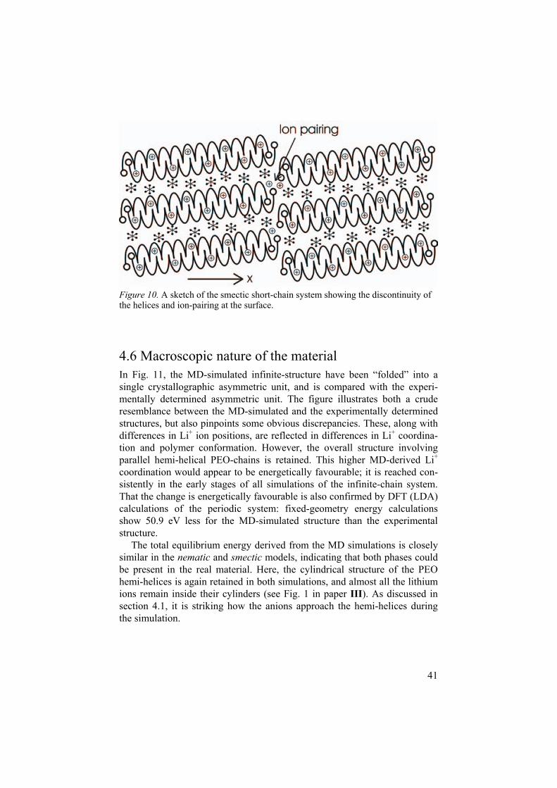
41

Figure 10. A sketch of the smectic short-chain system showing the discontinuity of the helices and ion-pairing at the surface.

4.6 Macroscopic nature of the materialIn Fig. 11, the MD-simulated infinite-structure have been “folded” into a single crystallographic asymmetric unit, and is compared with the experi-mentally determined asymmetric unit. The figure illustrates both a crude resemblance between the MD-simulated and the experimentally determined structures, but also pinpoints some obvious discrepancies. These, along with differences in Li+ ion positions, are reflected in differences in Li+ coordina-tion and polymer conformation. However, the overall structure involving parallel hemi-helical PEO-chains is retained. This higher MD-derived Li+

coordination would appear to be energetically favourable; it is reached con-sistently in the early stages of all simulations of the infinite-chain system. That the change is energetically favourable is also confirmed by DFT (LDA) calculations of the periodic system: fixed-geometry energy calculations show 50.9 eV less for the MD-simulated structure than the experimental structure.

The total equilibrium energy derived from the MD simulations is closely similar in the nematic and smectic models, indicating that both phases could be present in the real material. Here, the cylindrical structure of the PEO hemi-helices is again retained in both simulations, and almost all the lithium ions remain inside their cylinders (see Fig. 1 in paper III). As discussed in section 4.1, it is striking how the anions approach the hemi-helices during the simulation.

42

Figure 11. The “folded” asymmetric unit for the infinite-chain system (large spheres), compared with the crystallographically determined asymmetric unit (small spheres).

It can also be noted (as illustrated in Fig. 10), that the helical axes in the smectic model do not lie parallel to the x-direction but undergo a tilt which breaks the continuity of the short-chains across the space between the smec-tic layers. The lithium ions are thus less able to diffuse from helix to helix; likewise, the anions cannot move from channel to channel. This has a re-stricting effect on the conduction mechanism. The nematic model exhibits a somewhat different behaviour: the PEO cylinders now follow a common infinite polymer-chain axis, but each cylinder has a small kink (Fig. 12), giving the whole cylindrical structure a wave-like form. These kinks occur close to regions of PEO chain-breaking; either within the chain itself or in adjacent chains. The structural effect of a kink extends upto 10 Å from the kink itself. These structural features clearly imply that ion mobility will be different here compared to the infinite-chain system, since the lithium chan-nels within the helices and the anionic columns between the helices are sig-nificantly obstructed.

Figure 12. A double hemi-helix in the nematic model of the short-chain system with a typical kink circled.

43

4.7 Calculated diffraction profiles Although no effective asymmetric unit could be found for the short-chain systems, a significant level of periodicity nevertheless exists in the structure: the helices assemble in a regular way, and non-randomicity certainly exists in the distribution of the Li+ ions in the MD box. This justifies a closer com-parison of the MD- and experimentally-derived structures.

The effective diffraction pattern has been calculated directly from the atomic positions in the MD box using the program DISCUS [94]. The results are compared with the experimental diffractogram in Fig. 13. A minor prob-lem with this comparison is that the simulated structure is modelled using the parameters from a neutron diffraction study of a deuterated system; this will have slightly different cell parameters. Hence the small shifts in some peak positions.

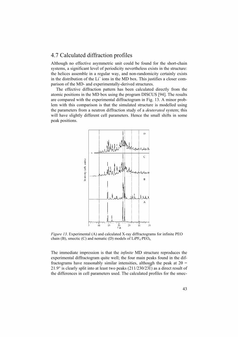
Figure 13. Experimental (A) and calculated X-ray diffractograms for infinite PEO chain (B), smectic (C) and nematic (D) models of LiPF6 PEO6.

The immediate impression is that the infinite MD structure reproduces the experimental diffractogram quite well; the four main peaks found in the dif-fractograms have reasonably similar intensities, although the peak at 2 = 21.9 is clearly split into at least two peaks (211/230/231) as a direct result of the differences in cell parameters used. The calculated profiles for the smec-

44

tic and nematic short-chain structures (which have the same Mw as the ex-perimental material) agree less well with experiment. Although the strongest experimental peaks are also dominant in the calculated diffractograms, the striking incidence of spurious noise peaks in the calculated the short-chain model profiles is disappointing. Apparently, the size of the MD box is totally inadequate to reproduce the infinitely periodic nature of a polymeric material of this type involving such a rich variety of conformations. In spite of this, the smectic model can be said to give the best overall agreement with ex-periment, since (if the noise level is disregarded) the relative intensities for the four main peaks in the experimental diffractogram are very well repro-duced. This can be taken as strong evidence that the smectic model best rep-resents the real short-chain material.

45

5. Dynamics

The MD simulations have also provided much information on the dynamicsin the system. These features will be summarised in the following chapter.

5.1 Thermal motion and displacement parametersThermal displacement parameters have been calculated for the different sys-tems from their atomic trajectories; see Table 4. We see that the MD-derived thermal displacement parameters lie significantly closer to the experimental values for pure PEO [36] than the unrealistically low constrained overall value used in the structural refinement of LiPF6 PEO6 [24].

Table 4. MD-derived isotropic thermal displacement parameters (Uiso in Å2) for different atom-types in the smectic, nematic and infinite-chain models.

Atom type Smectic model Nematic model Infinite PEO Li 0.051 0.047 0.037 P 0.061 0.061 0.051 F 0.519 0.552 0.127 C 0.076 0.070 0.076 O 0.060 0.057 0.050

The most dynamic feature of the simulated system (apparent from Table 4) involves the PF6

- anions, which are seen to behave as hindered rotators, with the individual fluorine atoms occasionally interchanging their positions. For the infinite-chain system, rotation of the anions is seen to occur predomi-nantly about the y- and z-axes, and to a lesser extent about the x-axis, which is the direction of the polymer chains. The atomic distributions of the F-atoms in the “folded” PF6

- ions are plotted in three different planes in Fig. 14. The extension of the F-distribution inward toward the central axis of the polymer hemi-helices (see Fig. 14b) is especially interesting; it could suggest two preferred PF6

- orientations which can, in turn, be related to the double-peaking seen in the polymer dihedral-angle distributions (Fig. 8b). The dis-tribution of orientations clearly also suggests the possibility of correlation between PF6

- rotation about axes perpendicular to the chain direction and Li+

propagation along the direction of the hemi-helices, i.e., a situation reminis-cent of a “paddle-wheel mechanism” [95], whereby anion rotation assists Li+

46

transport. However, these correlations have yet to been investigated in this work.

Figure 14. Atomic distribution in the xy- (a), xz- (b) and yz-planes (c) for the F atoms of the PF6

- ions in the MD simulation of infinite-chain LiPF6 PEO6.

Comparison of the different simulated systems shows a reasonable corre-spondence. Notably, the thermal parameters in the smectic and nematic sys-tems are essentially identical, and systematically larger than for the infinite system. Moreover, the MD simulation indicates significantly higher thermal motion in the F-atoms in the short-chain compared to the infinite systems, which clearly reflects the higher rotational freedom in the short-chain sys-tem. Apparently, in a system with a more relaxed polymer backbone, the anions are more free to rotate in all directions.

5.2 Ion hopping and conductivity All systems investigated exhibit ionic conductivity above a certain field strength. For the infinite-chain system, threshold values can be defined (these are listed in Table 3). The short-chain system behaves somewhat dif-ferently: ion transport can be detected at significantly lower field values, but the systems also displayed less tolerance to the strength of the applied field. Ion movement can be detected in the direction of the applied field already at such comparatively low value as 1 106 V/m for some of the systems.

As described in Chapter 2, conductivity can be calculated using the Nernst-Einstein equation and the diffusion coefficient extracted from the mean-square displacement of the ions in the simulation box. Such values are most unreliable, however, in view of the poor statistics of the simulations and the non-randomicity of the ionic motion under the influence of an im-posed electric field. Ion-jump frequencies can nevertheless be used for com-parison purposes; these are listed for structurally stable conducting systems in Tables 5 and 6.

47

Table 5. Ion-jump frequencies for infinite-chain systems (in jumps/ns).

System External

field/106 V/m

PF6- jump

frequency Li+ jump frequency

LiPF6 PEO6 5.0 120 0

SiF62-doped (distant from extra Li+) 4.0 140 3

SiF62-doped (close to extra Li+) 4.75 130 27

SF6 doped 4.0 150 0

SF6 doped 4.5 300 25

Table 6. Ion-jump frequencies for short-chain systems (in jumps/300 ps).

System Field/106 V/m

Li jumps < 4.5 Å

Li jumps > 4.5 Å

PF6- jumps

< 4.5 Å PF6

- jumps > 4.5 Å

1 0 0 1 0 2 1 0 2 0 Undoped3 7 8 11 2 1 0 0 1 0 2 2 0 3 1 SiF6

2--doped 3 11 0 7 1 1 1 0 0 0 2 2 0 2 0

Nematicmodel

SF6-doped 3 7 0 17 14 1 0 0 0 0 2 6 0 3 0 Undoped3 11 0 13 3 1 3 0 2 0 2 2 0 4 0

SiF62--doped

(bulk)3 7 0 9 4 1 1 0 1 0 2 9 0 5 1

SiF62--doped

(surface)3 11 0 5 8 1 1 0 1 0 2 8 0 3 0

Smectic model

SF6-doped 3 10 0 6 7

48

The conductivity is seen as ion jumps parallel to the hemi-helical axes. In the infinite-chain systems, the jumps are easily distinguished as long, simultane-ous anion jumps, whereby a PF6

- ion migrates into the position of its neigh-bour along an inter-helical anion column, or as shorter lithium ion jumps inside the helices. In the short-chain systems, long and short jumps occur for both ion types. This difference is due to the anion displacement in the yz-directions, which makes it possible for anions to move in the x-direction without pushing another anion ahead of it; the energy barrier is therefore much lower. The coupled motion in the anion column or the diffusion of cations from helix to helix is restricted in both the smectic and nematic sys-tems due to the discontinuity across the interface layer, or the kinks in the polymer cylinders, respectively.

As stated earlier, NMR studies of the LiXF6 PEO6 (X=Sb,P) systems have suggested that the conductivity is dominated by the movement of lith-ium ions, i.e., the lithium transport number (t+) is 1.0 [22]. In contrast to this, MD results from the infinite-chain system suggest that it is the anions which dominate the ionic motion, with t- close to 1.0. This is also implicit in the MD-simulated structure: the cations coordinate strongly to the two hemi-helical polymer chains, thereby holding them together, while the anions are free to rotate about at least two different axes, suggesting a weak interaction with the polymer.

Interestingly, the number of Li+ jumps increases significantly in the short-chain system compared to the infinite chain, in spite of the lower. It is clear that the higher polymer relaxation in the short-chain systems favours the Li+

transport.

5.3 Mechanisms Inspection of ion-hopping sequences gives information on the ion conduc-tion mechanisms. A clear correlation exists in both systems between ion transport and the displacement of the lithium and the anion perpendicular to the helical axis (see, for example, Fig. 9 in paper II).

In the infinite-chain system, these displacements are clearly coupled; ani-ons are seen to approach the polymer helix, while Li+ ions move out towards them in the anion column. Li+ ions thus create an available site for the ani-ons close to the polymer. The coordination of an anion to Li+ also releases one ether-oxygen from the Li+-coordination sphere, causing a small twist to occur in the polymer chain (see Fig. 15).

The mechanism for the Li+-ion jumps along the infinite-polymer channels is shown in Fig. 16. The Li+ ions jump a shorter distance (generally ~3 Å) compared to the PF6

- jumps of ~6 Å, generally moving from 6- to 5-fold coordinated positions, as the polymer chain twist to re-establish 6-fold coor-

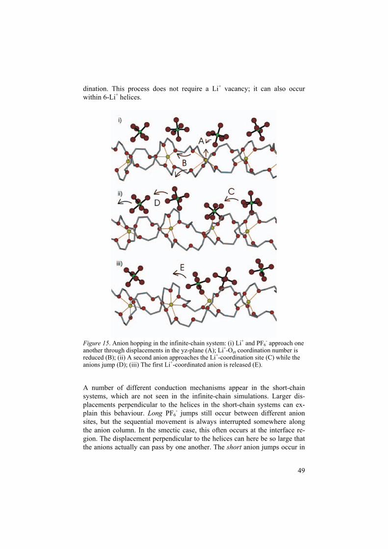
49

dination. This process does not require a Li+ vacancy; it can also occur within 6-Li+ helices.

Figure 15. Anion hopping in the infinite-chain system: (i) Li+ and PF6- approach one

another through displacements in the yz-plane (A); Li+-Oet coordination number is reduced (B); (ii) A second anion approaches the Li+-coordination site (C) while the anions jump (D); (iii) The first Li+-coordinated anion is released (E).

A number of different conduction mechanisms appear in the short-chain systems, which are not seen in the infinite-chain simulations. Larger dis-placements perpendicular to the helices in the short-chain systems can ex-plain this behaviour. Long PF6

- jumps still occur between different anion sites, but the sequential movement is always interrupted somewhere along the anion column. In the smectic case, this often occurs at the interface re-gion. The displacement perpendicular to the helices can here be so large that the anions actually can pass by one another. The short anion jumps occur in

50

a number of ways which are difficult to characterize systematically, but allinvolve one or two anions undergoing short anion jump in the yz-direction.

Figure 16. Li+ ion jumps in the infinite system: (i) A Li+ ion releases two ether oxy-gens (A) while moving into a 5-coordinated site (B); (ii) The lithium ion becomes 6-coordinated through motion of the polymer (C); (iii) This motion induces lithium shifts along the chain (D).

Because of the strong Li-Oet interaction, Li+ ions undergo fewer long jumps than the PF6 anions also in the short-chain systems. In one case here, how-ever, simultaneous long jump of all cations in a helix was actually seen. This simultaneous Li+ ion motion did coincide with nearby PF6

- ions jumps in the opposite direction, in a “paddle-wheel” type mechanism [95]. It is most in-teresting to note that such a mechanism is not dependent on a defect and, in fact, does not even occur in doped systems where vacancies or extra lithium ions are introduced.

51

In the smectic model, the end-group layer actually serves as a bottleneck for the conduction processes along the direction of the applied field through the formation of stable ion-pairs/clusters. Fewer ions migrate across this surface than within the “bulk” regions free from end-groups. Ion mobility is seen, however, within the surface of this region, perpendicular to the direc-tion of the applied field.

5.4 The effects of doping It is obvious clear Table 5 that aliovalent doping has some influence on ionic conductivity in the infinite-chain systems; in good agreement with experi-ment. Interestingly, this would not appear to be the result of Li+-ion migra-tion across a vacancy within the polymer channels, or of an extra Li+-ionbeing pushed along the double hemi-helix. It follows rather from a dopant-induced rearrangement of the anions and cations in the yz-plane, facilitating the conduction mechanisms described above.

The effect of doping on ion conduction is less clear, however, in the short-chain systems (see Table 6). Indeed, for fields as high as 3 106 V/m, all systems display relatively high conductivity irrespective of dopant.

The only significantly higher conductivity in a short-chain system is found in the nematic model doped with SF6. The observed effect follows from PF6

- migration close to the uncharged SF6 dopant. This creates an anionvacancy in an adjacent inter-helical column, leading to the observed conduc-tivity enhancement, compared to the other simulated systems.

The SiF62- dopants do not participate in the conduction process, but re-

main stable throughout the simulations of the short-chain systems. Instead, an increase in anion jump frequency can be identified in these systems close the extra charge compensating lithium. It migrates out towards the surface of its hemi-helix where it promotes anion conductivity through the familiar displacement this induces in the yz-plane for the neighbouring anions. This clearly resembles the effect of doping seen the infinite system, suggesting that doping should also have a positive effect in short-chain systems.

5.5 Long-chain vs. short-chain effects The chain-ends clearly display more dynamical behaviour than the rest of the polymer, which can be seen from the MSD-plots for the carbon atoms (see Fig. 4 in paper III), where it is apparent that the diffusion of end-group car-bons is larger than that for other backbone atoms. The end-groups in the smectic model are also more mobile. This is probably a surface phenome-non; there is more space available in the interface regions between the smec-tic layers, so the chain-ends can move around more freely. Ion mobility in

52

this surface region is also a real possibility, which is not probed here. We would have needed to impose the electric field perpendicular to the chain direction.

Not surprisingly, it can also be noted that atoms in the short chains move more freely than those in the infinite chains. This can indicate a high degree of chain relaxation, and is consistent with the higher observed t+(Li): the flexibility of the low molecular-weight polymer chain facilitates ionic trans-port.

53

6. Concluding remarks – MD vs. experiment

The infinite-chain structure resulting from the MD simulation compares reasonably well with experiment. The different coordination number and dihedral angle distribution could well be correct; the quality of the experi-mental data used for the structure determination was poor, and it was used to refine a large number of structural parameters. Indeed, our derived MD model actually reproduced the experimental diffraction pattern quite well, considering the limited box-size and simulation times used. It is more prob-lematical that the derived transport numbers disagree so dramatically for the infinite-chain model compared to the experimental NMR results. That t+ is as high as 1.0 is based on the observed narrowing of the 7Li peak with tempera-ture (suggesting high Li+ dynamics, but not necessarily lithium transport) and a coupling between the 1H and the 31P signals (suggesting that the PF6

-

movement is coupled to the movement of the polymer chain). Such data need not contradict the MD simulation results; the polymer hydrogens pro-trude from the hemi-helices, and are thus strongly coupled to anion move-ment. Furthermore, dominant lithium migration within the polymer channels fails to explain conductivity dependence on anion-type. Transport numbers should thus be investigated further, before any final conclusions are drawn.

It is more encouraging that our infinite-chain model well reproduces the effects of doping well, and also provides a credible explanation for the en-hancment effect of aliovalent doping on conductivity.

However, infinite-chain models (both experimental and MD-generated) neglect the existence of polymer end-groups, their possible registry and their influence on the conduction mechanism. Our MD simulations show a dra-matic impact on both structure and dynamics for a molecular weight as low as 1000. Structurally, the shortening of the polymer chain leads to quite dif-ferent PEO chain conformations which, in turn, facilitates different modes of ion-pairing. It can also change the macroscopic nature of the material – be-coming discontinuous in the smectic model, or wave-like in the nematic. These features are totally absent from both the experimental or the infinite-chain models.

One might expect that lowering the molecular weight would give better agreement with the calculated diffraction profile; after all, a low molecular weight was used in the X-ray diffraction experiment. This would not seem to be the case; neither of the short-chain models reproduces the experimental data noticeably better than the well-ordered infinite-chain model. However,

54

the short time-span of the simulations and the small size of the MD box ap-pear to limit the quality of the calculated diffraction profiles.

Turning to the dynamical aspects of the study, we see that the short-chain systems better reproduce the Li+ ion conductivity suggested from experi-ment, although the transport number t+ (0.4) is still far less than 1.0. Further, this higher Li+ transport number would seem to be coupled to the polymer-chain relaxation and the discontinuity of the anion channels – effects which are clearly related to the lower molecular weight.

The results from MD simulations presented in this thesis do not say which model best represents the real material – the smectic, the nematic or the infi-nite-chain model. On the other hand, some very clear indications are given: especially that the effects of low molecular weight and the presence of end-groups must be taken into account in our models. Thus, although an infinite system fairly well reproduces some of the features of the experimental model and even the experimental diffraction profile, it nevertheless lacks the impor-tant features of the real material. The infinite-chain model has been of some help, however, in understanding ionic conductivity in crystalline polymer electrolytes: it has provided vital information on a number of structural and dynamical features: coordination, backbone conformation, anion dynamics, conduction mechanism and the rôle of dopants.

Of the two short-chain models, the majority of the results presented here would suggest the smectic to be preferred. Indeed, a smectic model is fa-voured from a structural chemistry viewpoint; short polymers tend to align in nature, e.g., in biological membranes. Macromolecular biological layers also display the same type of tilt seen in the smectic model of LiPF6 PEO6. It is even possible that the enhanced conductivity in the LiPF6 PEO6 system actu-ally occurs in the surfaces of these smectic layers, and was not detected in the simulations because the electric field was imposed along and not perpen-dicular to the chain direction.

55

Acknowledgements

First of all, I would like to thank my supervisor Professor Josh Thomas. His unending support, enthusiasm, generosity and, of course, his vast scientific knowledge and perspectives on Chemistry has helped me accomplish this thesis more than anything else. His struggle with my written and spoken English has also been invaluable. Josh, you are the best guide a student can have into the World of scientific research!

Alvo Aabloo, my MD guru in Tartu, is warmly acknowledged; as is my previous supervisor Mattias Klintenberg, who introduced me to computa-tional chemistry and spent a lot of time teaching me in the fields of Optics and Atom physics. We also had some good times at both sides of the Atlan-tic.

Anti! Your impact on this work has been profound. I don’t know what I would have done without you and your programming skills. I will be ever grateful for the time you spent on this project, especially towards the end. The rest of the Estonian crew – Heiki, Andi, Jaanus – are also gratefully acknowledged for their help, and for the interesting discussions and fun times we have had.

The Department of Materials Chemistry has been a friendly place to work all these years: scientist and non-scientists have all been fantastic. The Struc-ture and Dynamics Group and The Ångström Advanced Battery Centre have been an enlightening research environment. Past and present PhD students: Anton (my friend for almost 30 years!), Jonas (who started at Kemikum together with me), Hanna (and her family!), Anders (for all the lunches at Rullan), Sara (my friendly room-mate since we started here) and many more – you have made the years here even better.

Ett tack till alla mina andra vänner, utanför institutionen (ni vet vilka ni är!). Mina år som både student och doktorand har varit några av de absolut bästa man kan ha, och ni har alla en plats i mitt hjärta.

Ett stort tack riktas också självklart till mina föräldrar, mina bröder och övriga släkten. Den varma atmosfär ni utgör är ett av mina största stöd.

Slutligen, Malin – tack för all kärlek och omtanke. Du är bäst!

Uppsala – 17 March 2005

56

Populärvetenskaplig sammanfattning

Att förstå jonledning i kristallina polymerelektrolyter

Energikällor och energilagring Vi står inför stora utmaningar på energiforskningens område. De politiska beslutsfattarna på både global och lokal nivå har beslutat att skära ned på användingen av fossila bränslen – dels för att de släpper ut växthusgaser, och dels för att de inte är förnyelsebara naturresurser. De kommer, om använd-ningen av dem fortsätter, de facto att ta slut så småningom.

Bland de alternativa energikällor forskarsamhället fokuserar på är sol- och bränsleceller de som anses ha bäst förutsättningar att bygga upp vår framtida energiförsörjning. Men även frågan om att på ett effektivt och miljövänligt sätt lagra energi kommer att vara viktigt.

Jonledningsförmågan i litium-polymerbatteriet Ett sätt att lagra energi kemiskt är med hjälp av batterier. Litiumjonbatteriet, som introducerades på 1990-talet, kombinerar hög spänning och hög energi-täthet med god säkerhet och förmågan att vara återuppladdningsbar. Idag används batteriet i mobiltelefoner och bärbara datorer, men dess använd-ningsområde kan förhoppningsvis utvidgas.

Som alla batterier består litiumjonbatteiret av en anod, en katod och en mellanliggande elektrolyt – dvs två elektriska poler, samt ett material emel-lan dessa. När de negativa elektronerna vandrar genom en ledning från ano-den till katoden, så kompenseras detta elektriskt med att positivt laddade atomer, joner, också slussas från anod till katod genom elektrolyten (se Figur 1 i den engelskspråkiga texten). Det är så batteriet genererar elektricitet. I litiumjon-polymerbatteriet är jonerna litiumjoner, Li+, och elektrolyten be-står av så kallade polymerer – långa, kedjeliknande molekyler.

Ett problem med polymerelektrolyter har varit att de slussar dessa joner relativt dåligt. Detta har länge ansetts bero på att polymeren gärna bildar kristallina, det vill säga välordnande, faser, medan flera studier tyder på att jonledningen främst försigår i den oordnade, eller den “amorfa” fasen. Fors-karsamhället har följdaktligen spenderat mycket tid (och pengar) på att utöka

57

den amorfa fasen i materialet. Trots detta verkade det som att forskningen under 1990-talet slog i taket för hur mycket man kunde öka jonledningsför-mågan utan att göra avkall på säkerheten hos batteriet.

LiPF6 PEO6

År 2001 publicerades emellertid en studie som kastade om perspektiven något. En typ av polymerelektrolyter, LiXF6 PEO6 (där X = P, As, eller Sb), uppvisade högre ledningsförmåga i sin kristallina fas än i sin amorfa – även om jonledningen ändå var ganska låg. Eftersom andra studier visar att poly-meren behåller mycket av sin lokala struktur när den går in i sin amorfa, oordnade fas, så menade vissa forskare att utvidgade studier av de kristallina polymerelektrolyterna kanske kunde visa vägen mot högre jonledningsför-måga.

Den relativt goda jonledningsförmågan hos LiXF6 PEO6 har ansetts bero på den ganska speciella strukturen hos materialet (se Figur 2 i den engelsk-språkiga texten). Polymeren – i det här fallet poly(etylenoxid), PEO – forme-rar sig på den molekylära nivån i en cylinderlikande konstruktion, som inne-sluter de positiva litiumjonerna. De negativa XF6

--jonerna separeras då från litium, och denna separation av jonslagen anses generellt ge en positiv effekt på ledningsförmågan – att joner parar sig med varandra i elektrolyten har ansetts vara ett problem i de material som används idag. Ytterligare studier med så kallad magnetisk kärnspinnsresonans (NMR) tyder på att det är liti-umjonen som står för jontransporten i materialen. Skulle detta vara fallet, så skulle det vara gynsamt för tillämpningar i batterier.

I den här doktorsavhandlingen presenteras en rad studier av kristallint LiPF6 PEO6 gjorda med molekyldynamik (MD). Detta är de första studierna av dessa material med den tekniken.

Molekyldynamik (MD) Molekyldynamik är en beräkningsteknik för att simulera hur atomer och molekyler interagerar med varandra under en relativt kort tidrymd (oftast upp till någon miljarddels sekund). Man tillskriver initialt alla atomerna i sitt tänkta system (ofta bara några tusentals atomer) en viss massa och en viss beskrivning för hur de ska interagera med varandra. Med hjälp av detta kan man beräkna hur atomerna kommer att förflytta sig undan för undan under simuleringen. Matematiken är densamma som Isaac Newton formulerade redan på 1600-talet i sitt klassiska verk Principia Mathematica, men efter-som det är tusentals ekvationer att lösa om och om igen tar man datorer till hjälp. På detta sätt generar man en kort filmsekvens över hur materialet beter sig. Hur resultatet blir beror på hur väl man lyckats beskriva interaktionerna mellan partiklarna – detta är oftast det mest problematiska med metodiken.

58

ResultatEftersom man inte med mikroskop kan se atomstrukturen i ett material som LiPF6 PEO6, så måste man ta till andra medel för att undersöka denna. I arti-kel I presenteras en analys av hur strukturen hos MD-simulerat LiPF6 PEO6tedde sig jämfört med den struktur som experimentalisterna kommit fram till med så kallade diffraktionsstudier. Det visade sig att den överensstämde ganska bra: litium koordinera förvisso i genomsnitt 6 syre-atomer från po-lymeren i simuleringen, till skillnad från 5 i den experimentellt föreslagna strukturen, och polymerens struktur var något annorlunda, men den cylinder-formade polymerformationen och separationen mellan Li+ och PF6

- kvarstod. Emellertid kunde ingen transport av joner skönjas i systemet, så det gick inte att dra några slutsatser om jonledningen.

För att kunna studera den essentiella jonledningen i materialet så lades en serie elektriska fält över det simulerade systemet i artikel II. Vidare under-söktes hur materialet betedde sig om en liten del av PF6

--jonerna byttes ut mot molekyler med annan laddning, SiF6

2- eller SF6, så kallad dopning. Det visade sig att viss jonledning kunde iakttas här, men i motsättning till de experimentella NMR-studierna visade undersökningen att det var de negati-va PF6

--jonerna som stod för det mesta av laddningstransporten. Angående dopningen, iakttogs att den fick gynnsam effekt på jonledningsförmågan, något som också förutsagts av experimentella studier.

I både artikel I och II fanns sålunda en del skillnader mellan dessa simu-leringsstudier, och de resultat som experimenten visar. Det är givetvis natur-ligt att då ställa sig frågan om vilkendera modell som är rätt och fel, men för detta behövs mer forskning – det är inte säkert att experimentella data har tolkats rätt. En sak som är “fel” i båda modellerna av materialet, är att poly-merens längd och dess änd-grupper negligerats.

I artikel III undersöktes sålunda vilka strukturella skillnader som uppstod i materialet om polymerkedjorna kortades till enbart 23 enheter. I de tidigare simuleringarna, likväl som de modeller experimentalisterna begagnat sig av, hade det förutsatts att polymererna var oändliga; något som inte överens-stämmer med verkligheten. 23 PEO-enheter svarar mot en molekylvikt som använts i flera av de experimentella studierna. Det visade sig att förkortandet av polymerkedjan gav upphov till mer oordnade konformationer i materialet. Polymeren, som nu blev väl kort för att kallas “poly”-mer, började anta en rad olika konfigurationer. Samtidigt närmade sig de negativa PF6

--jonerna de positiva Li+-jonerna i helixarna. Denna strukturella studie pekade mot att jonledningen skulle påverkas avsevärt av dessa skillnader.

I artikel IV, slutligen, så studerades hur LiPF6 PEO6 med korta polymer-kedjor, alltså det “riktiga” materialet, transporterade joner under ett pålagt elektriskt fält över simuleringsboxen. I korthet kan man säga att metoderna för artikel II tillämpades på materialet i artikel III. Här framkom det att jon-ledningen fungerade aningen annorlunda än i simuleringarna med oändliga

59

polymerkedjor: bland annat var det jämförelsevis fler positiva litiumjoner som transporterades genom simuleringsboxen. Detta verkar främst bero på att polymerens flexibilitet ökat när den kortats till 23 enheter. Denna flexibi-litetet kan tänkas möjliggöra transport av litium på sätt som påminner om situationen i oordnade, amorfa material – de som tidigare ansätts ha de bästa egenskaperna för jonledning.

SlutsatserPå en rad olika sätt har de fyra uppsatserna bidragit till att öka förståelsen av både strukturen och dynamiken hos den kristallina polymerelektrolyten LiPF6 PEO6. En del data pekar på att det är viktigt att ta hänsyn till molekyl-vikten och änd-grupperna för att till fullo förstå hur jonlendingen i dessa material fungerar. Men även det simulerade systemet med oändliga polyme-rer har bidragit till att berätta hur materialen ser ut och beter sig på en atomär nivå. Molekyldynamik (MD) har visat sig vara ett effektivt verktyg i studiet av jonledningsprocesserna, och kan säkerligen användas i utvidgade studier.

60

References

[1] C.J. Campbell, “The Assessment and Importance of Oil Depletion”, Paper at the Interna-tional Workshop on Oil Depletion, Uppsala University, 2002.

[2] C.J. Campbell and J.H. Laherrère, Scientific American, March 1998. [3] M. Grätzel, Nature, 414 (2001) 338. [4] B.C.H. Steel and A. Heinzel, Nature, 414 (2001) 345. [5] J.M. Tarascon and M. Armand, Nature, 414 (2001) 359. [6] W.A. van Schalwijk and B. Scrosati, Advances in Lithium-Ion Batteries, Kluwer Aca-

demic/Plenum Publishers, New York, 2002. [7] M. Winter, J.O Besenhard, M.E. Spahar and P. Novák, Adv. Mater., 10 (1998) 725. [8] H. Shirakawa, E.J. Louis, A.G. MacDiarmid, C.K. Chiang and A.J. Heeger, J. Chem. Soc.

Chem. Comm. (1977) 579. [9] F.M. Gray, Polymer Electrolytes, The Royal Society of Chemistry, Cambridge, 1997. [10] P.G. Bruce, Solid State Electrolytes, Cambridge University Press, Cambridge, 1995. [11] D. Benrabah, J-Y. Sanchez and M. Armand, Solid State Ionics, 60 (1993) 87. [12] D. Benrabah, J-Y. Sanchez, D. Deroo and M. Armand, Solid State Ionics, 70/71 (1994)

157.[13] C. Chintapalli and R. Frech, Solid State Ionics, 86-88 (1996) 341. [14] M.M. Silva, S.C. Barros, M.J. Smith, J.R. MacCallum, J. Power Sources, 111 (2002) 52. [15] F. Croce, G.B. Appetecchi, L. Persi and B. Scrosati, Nature 394 (1998) 456. [16] W. Krawiec, L.G. Scanlon, Jr., J.P. Fellner, R.A. Vaia, S. Vasudevan and E.P Giannelis,

J. Power Sources, 54 (1995) 310. [17] D. Golodnitsky, G. Ardel and E. Peled, Solid State Ionics, 147 (2002) 141. [18] A. Reiche, A. Weinkauf, B. Sander, F. Rittig and G. Fleischer,

Electrochim. Acta, 45 (2000) 1327. [19] Y. Aihara, S. Arai and K. Hayamizu, Electrochim. Acta, 45 (2000) 1321. [20] M.A.S.A. Samir, F. Alloin, J.-Y. Sanchez and A. Dufresne, Macromolecules, 37 (2004)

4839.[21] L. Ding, Polymer, 38 (1997) 4267. [22] Z. Gadjourova, Y.G. Andreev, D.P. Tunstall and P.G. Bruce,

Nature, 412 (2001) 520. [23] G.S. MacGlashan, Y.G. Andreev and P.G. Bruce, Nature, 398 (1999) 792. [24] Z. Gadjourova, D. Matrín y Marero, K.H. Andersen, Y.G. Andreev and P.G. Bruce,

Chem. Mater., 13 (2001) 1282. [25] D.E. Fenton, J.M. Parker and P.V. Wright, Polymer, 14 (1973) 589. [26] P. V. Wright, Br. Polym. J., 7 (1975) 319.

61

[27] M. Armand, J.M. Chabagno and M. Duclot in Second International Meeting on Solid Electrolytes (extended abstracts), C.A. Vincent (ed.), St. Andrews University Press, Scotland, 1978.

[28] M.B. Armand, J.M. Chabagno and M.J. Duclot in Fast Ion Transport in Solids, P Vash-ista, J.N. Mundy and G.K. Shenoy (eds.), Elsevier, New York, 1979.

[29] D. Linden, Handbook of Batteries, McGraw-Hill, New York, 1994. [30] S. Gottesfeld and T. Zawodzinski in Advances in Electrochemical Science and Engineer-

ing, R.C. Alkire, H. Gerischer, D.M Kolb and C.W. Tobias, Wiley-VCH Verlag, Wein-heim, 1997.

[31] M. Armand and M. Gauthier in High Conductivity Solid Ion Conductors, T. Takahashi (ed.), World Scientific Press, Singapore, 1989.

[32] G. Cameron and M.D. Ingram in Polymer Electrolytes Reviews-2, J.R MacCallum and C.A. Vincent (eds.), Elsevier, London, 1989.

[33] L.A. Dominey, Lithium Batteries: New Materials, developments and Perspectives, G. Pistoia (ed.), Elsevier, 1994.

[34] M.S. Mendolia and G.C. Farrington, Adv. Chem. Ser., 245 (1995) 107. [35] J.M.G. Cowie and S.H. Cree, Ann. Rev. Phys. Chem., 40 (1989) 85. [36] Y. Takahashi and H. Tadokoro, Macromolecules, 6 (1973) 672. [37] M. Watanabe and N. Ogata, in Polymer Electrolytes Reviews-1, J.R MacCallum and C.A.

Vincent (eds.), Elsevier, London, 1987. [38] J. Przyluski and W. Wieczorek, Solid State Ionics, 53-56 (1992) 1071. [39] R. Huq, G.C. Farrington, R. Koksbang and P.E. Tonder, Solid State Ionics, 57 (1992)

277.[40] C.A. Vincent, Electrochim. Acta, 40 (1995) 2035. [41] M. Armand, W. Gorecki and R. Andréani in Second International Symposium on Poly-

mer Electrolytes, B Scrosati (ed.), Elsevier, London, 1990. [42] C. Berthier, W. Gorecki, M. Minier, M.B. Armand, J.M. Chabagno and P. Rigaud, Solid

State Ionics, 11 (1983) 91. [43] S.D. Druger, A. Nitzan and M.A. Ratner, J. Chem. Phys., 79 (1983) 3133. [44] P.G. Bruce and C.A. Vincent, J. Chem. Soc. Faraday Trans., 89 (1993) 3187. [45] G.C. Farrington and R.G. Linford in Polymer Electrolytes Reviews-2, J.R MacCallum

and C.A. Vincent (eds.), Elsevier, London, 1989. [46] M.A. Ratner in in Polymer Electrolytes Reviews-1, J.R MacCallum and C.A. Vincent

(eds.), Elsevier, London, 1987. [47] M. Armand in Polymer Electrolytes Reviews-1, J.R MacCallum and C.A. Vincent (eds.),

Elsevier, London, 1987. [48] Y.G. Andreev and P.G. Bruce, J. Phys.: Condens. Matter, 13 (2001) 8245. [49] R. Frech, S. Chintapalli, P.G. Bruce, C.A. Vincent, J. Chem. Soc. Chem. Commun.

(1997) 157. [50] Y.G. Andreev, P. Lightfoot and P.G. Bruce, J. Appl. Cryst., 30 (1997) 294. [51] R. Iwamoto, Y.Saito, H. Ishihara, H. Tadokoro, J. Polym. Sci. Part A-2, 6 (1968) 1509. [52] T. Hibma, Solid State Ionics, 9/10 (1983) 1101. [53] P. Lightfoot, J.L. Nowinski and P.G. Bruce, J. Am. Chem. Soc., 116 (1994) 7469. [54] Y. Chatani and S. Okamura, Polymer, 28 (1987) 1815.

62

[55] Y. Chatani, Y. Fujii, T. Takayanagi and A. Honma, Polymer, 31 (1990) 2238. [56] Y.G. Andreev, G.S. MacGlashan and P.G. Bruce, Phys. Rev. B, 55 (1997) 12011. [57] G.S. MacGlashan, Y.G. Andreev and P.G. Bruce, J. Chem. Soc. Dalton Trans. (1998)

1073.[58] P. Lightfoot, M.A. Mehta and P.G. Bruce, J. Mater. Chem. 2 (1992) 379. [59] P. Lightfoot, M.A. Mehta and P.G. Bruce, Science, 262 (1993) 883. [60] Y.G. Andreev, P. Lightfoot and P.G. Bruce, J. Chem. Soc. Chem. Comm. (1996) 2169. [61] Y.G. Andreev, V. Seneviratne, M. Khan, W.A. Henderson, R.E. Frech and P.G. Bruce,

Chem. Mater., 17 (2005) 767. [62] I. Martin-Litas, Y.G. Andreev and P.G. Bruce, Chem. Mater., 14 (2002) 2166. [63] J.B Thomson, P. Lightfoot and P.G. Bruce, Solid State Ionics, 85 (1996) 203. [64] E. Staunton, A.M. Christie, I. Martin-Litas, Y.G. Andreev, A.M.Z. Slawin and P.G.

Bruce, Angew. Chem. Int. Ed., 48 (2004) 2103. [65] W. A. Henderson and S. Passerini, Electrochem. Commun., 5 (2003) 575. [66] E. Staunton, A.M. Christie, Y.G. Andreev, A.M.Z. Slawin and P.G. Bruce, J. Chem. Soc.

Chem. Commun. (2004) 148. [67] Y. Andreev and P.G. Bruce, Electrochim. Acta, 45 (2000) 1417. [68] D. Golodnitsky and E. Peled, Electrochim. Acta, 45 (2000) 1431.[69] P.V. Wright, Y. Zheng, D. Bhatt, T. Richardson and G. Ungar, Polym. Int., 47 (1998) 34. [70] S.M. Kelly, Materials Science of Liquid Crystals, Taylor & Francis, London, 2003. [71] A.M. Christie, S.J Lilley, E. Staunton, Y.G. Andreev and P.G. Bruce,

Nature, 433 (2005) 50. [72] P.G. Bruce, The 12th International Meeting on Lithium Batteries (IMBL-12), Nara, Japan,

27 June – 2 July 2004. [73] Z. Stoeva, I. Martin-Litas, E. Staunton, Y.G. Andreev and P.G. Bruce,

J. Am. Chem. Soc., 125 (2003) 4619. [74] V. Seneviratne, R. Frech and J.E. Frenaux, Electrochim. Acta, 48 (2003) 2221. [75] P.G. Bruce, private communications. [76] L.A. Curtiss and M.S. Gordon (eds.), Computational materials chemistry: methods and

applications, Kluwer, London, 2004. [77] M.P. Allen and D.J. Tildesley, Computer Simulation of Liquids, Oxford University Press,

1989.[78] J.M. Haile, Molecular Dynamics Simulation, Wiley, 1997. [79] E.A. Colbourn, Computer Simulation of Polymers, Longman Scientific & Technical,

1994.[80] D.C. Rapaport, The Art of Molecular Dynamics Simulation, Cambridge University Press,

1995.[81] S. Neyertz, D. Brown and J.O. Thomas, J. Chem. Phys., 101 (1994) 10064. [82] S.P. Gejji, J. Tegenfeldt and J. Lindgren, Chem. Phys. Lett., 226 (1994) 427. [83] F. Müller-Plathe, Acta Polymer., 45 (1994) 259. [84] O. Borodin and G.D. Smith, J. Phys. Chem., 107 (2003) 6801. [85] O. Borodin, G.D. Smith and R.L. Jaffe, J. Comp. Chem., 22 (2001) 641. [86] O. Borodin and G.D. Smith, Macromolecules, 31 (1998) 8396. [87] O. Borodin and G.D. Smith, Macromolecules, 33 (2000) 2273.

63

[88] A. Liivat, A. Aabloo and J.O. Thomas, J. Comp. Chem. In press. [89] K.E. Kinney, S. Xu and L.S. Bartell, J. Phys. Chem. 100 (1996) 6935. [90] M.A. Zendejas, Molecular Dynamics Simulation of Ionic Conduction in Solids, Thesis,

Uppsala University, 1994. [91] R. Frech, V. Seneviratne, Z. Gadjourova and P.G. Bruce, J. Phys. Chem., 107 (2003)

11255.[92] J.E. Mark and P.J. Flory, J. Am. Chem. Soc., 87 (1965) 1415. [93] A. Abe and J.E. Mark, J. Am. Chem. Soc., 98 (1976) 6468. [94] Th. Proffen and R.B. Neder, J. Appl. Cryst., 30 (1997) 171. [95] R. Kaber, L. Nilsson, N.H. Andersen, A. Lundén and J.O. Thomas, J. Phys.: Condens.

Matter., 4 (1992) 1925.

Acta Universitatis UpsaliensisDigital Comprehensive Summaries of Uppsala Dissertationsfrom the Faculty of Science and Technology 34

Editor: The Dean of the Faculty of Science and Technology

A doctoral dissertation from the Faculty of Science and Technology, Uppsala University, is usually a summary of a number of papers. A few copies of the complete dissertation are kept at major Swedish research libraries, while the summary alone is distributed internationally through the series Digital Comprehensive Summaries of Uppsala Dissertations from the Faculty of Science and Technology. (Prior to January, 2005, the series was published under the title "Comprehensive Summaries of Uppsala Dissertations from the Faculty of Science and Technology".)

Distribution: publications.uu.seurn:nbn:se:uu:diva-5734

ACTAUNIVERSITATIS

UPSALIENSISUPPSALA

2005