kalman filter
TRANSCRIPT
Kalman Filter
Man-Wai MAK
Dept. of Electronic and Information Engineering, The Hong Kong Polytechnic Universityhttp://www.eie.polyu.edu.hk/~mwmak
References:
S. Gannot and A. Yeredor, “The Kalman Filter”, Springer Handbook of SpeechProcessing, J. Benesty, M.M. Sondhi and Y. Huang (Eds.), Springer, 2008.
R. Faragher, “Understanding the Basis of the Kalman Filter Via a Simple and IntuitiveDerivation”, IEEE Signal Processing Magazine, Sept. 2012.
E. Benhamou, “Kalman filter demystified: from intuition to probabilistic graphical modelto real case in financial markets.” Available at SSRN 3292762 (2018).
https://www.youtube.com/watch?v=mwn8xhgNpFY
https://www.youtube.com/watch?v=4OerJmPpkRg
https://www.youtube.com/watch?v=ul3u2yLPwU0
http://www.bzarg.com/p/how-a-kalman-filter-works-in-pictures
https://www.youtube.com/watch?v=CaCcOwJPytQ
https://www.kalmanfilter.net/kalman1d.html
December 6, 2020
Man-Wai MAK (EIE) Kalman Filter December 6, 2020 1 / 25
Overview
1 What is Kalman Filter
2 Areas of Applications
3 Kalman Filter Formulations
4 1-Dimensional Example
Man-Wai MAK (EIE) Kalman Filter December 6, 2020 2 / 25
What is Kalman Filter
In a nutshell, a Kalman filter is a method for predicting the futurestate of a system based on previous ones.
Named after Rudolf E. Kalman in the 60’s, the Kalman filter is one ofthe most important and common data fusion algorithms in use today.
The most famous early use of the Kalman filter was in the Apollonavigation computer that took Neil Armstrong to the moon.
The Kalman filter has found numerous applications in fields related tocontrol of dynamical systems, e.g., predicting the trajectory ofcelestial bodies, missiles, and human poses.
Kalman filters are at work in satellite navigation devices, smart phone,and UAV.
Kalman filters are related to hidden Markov models but their latentvariables are continuous and their observed variables have a Gaussiandistribution (Benhamou, 2018).
Man-Wai MAK (EIE) Kalman Filter December 6, 2020 3 / 25
Areas of Applications
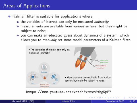
Kalman filter is suitable for applications where
the variables of interest can only be measured indirectly;measurements are available from various sensors, but they might besubject to noise;you can make an educated guess about dynamics of a system, whichallows you to manually set some model parameters of a Kalman filter.
https://www.youtube.com/watch?v=mwn8xhgNpFY
Man-Wai MAK (EIE) Kalman Filter December 6, 2020 4 / 25
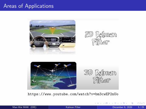
Areas of Applications
https://www.youtube.com/watch?v=bm3cwEP2nUo
Man-Wai MAK (EIE) Kalman Filter December 6, 2020 5 / 25
Intuitive Example
IEEE SIGNAL PROCESSING MAGAZINE [131] SEPTEMBER 2012
At t = 1, we also make a measure-ment of the location of the train using the radio positioning system, and this is represented by the blue Gaussian pdf in Figure 4. The best estimate we can make of the location of the train is provided by combining our knowledge from the pre-diction and the measurement. This is achieved by multiplying the two corre-sponding pdfs together. This is repre-sented by the green pdf in Figure 5.
A key property of the Gaussian function is exploited at this point: the product of two Gaussian functions is another Gaussian function. This is critical as it permits an endless number of Gaussian pdfs to be multiplied over time, but the resulting function does not increase in complexity or number of terms; after each time epoch the new pdf is fully represented by a Gaussian function. This is the key to the elegant recursive properties of the Kalman filter.
The stages described above in the fig-ures are now considered again mathe-matically to derive the Kalman filter measurement update equations.
The prediction pdf represented by the red Gaussian function in Figure 3 is given by the equation
( )y r e2
1; ,( )r
1 1 112 2 1
21
2
_
rn v
vv
n-
-
. (8)
The measurement pdf represented by the blue Gaussian function in Figure 4 is given by
( )y r e2
1; ,( )r
2 2 222 2 2
22
2
_vr
nv
v
n-
-
. (9)
The information provided by these two pdfs is fused by multiplying the two together, i.e., considering the prediction and the measurement together (see Figure 5). The new pdf representing the fusion of the
information from the prediction and mea-surement, and our best current estimate of the system, is therefore given by the prod-uct of these two Gaussian functions
( , )
.
y r
e
,
21
21
21
; ,( ) ( )
( (
r r
r r
1 1 2 2
12 2
22 2
12
22 2 2
fused
) )
121
2
222
2
121
2222 2
r r
r
n v n v
v v
v v=
v
n
v
n
v
n
v
n
--
--
--
+-
e e#=
e o
(10)
The quadratic terms in this new function can expanded and then the whole expression rewritten in Gaussian form
( )r n-
( )
2
y r
1
; ,
2 2
fused fused fused
fused
2
2
fused
fused
r
n v
vv
-e= , (11)
where
( )
12
22
1 22
2 12
112
22
12
2 1
fusednv v
n v n v
nv v
v n n
=+
+
= ++
-
(12)
and
2
12
22
12
22
12
12
22
14
fusedvv v
v vv
v v
v=
+= -
+.
(13)
These last two equations represent the measurement update steps of the Kalman filter algorithm, as will be shown explicitly below. However, to present a more general case, we need to consider an extension to this example.
In the example above, it was assumed that the predictions and measurements were made in the same coordinate frame and in the same units. This has resulted in a particularly concise pair of
??????
Measurement (Noisy)
Prediction (Estimate)
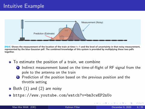
[FIG4] Shows the measur ement of the location of the train at time t = 1 and the level of uncertainty in that noisy measurement, represented by the blue Gaussian pdf. The combined knowledge of this system is provided by multiplying these two pdfs together.
???
Measurement (Noisy)
Prediction (Estimate)
[FIG5] Shows the new pdf (green) generated by multiplying the pdfs associated with the prediction and measurement of the train’s location at time t = 1. This new pdf provides the best estimate of the location of the train, by fusing the data from the prediction and the measurement.
A KEY PROPERTY OF THE GAUSSIAN FUNCTION IS
EXPLOITED AT THIS POINT: THE PRODUCT OF TWO GAUSSIAN FUNCTIONS IS ANOTHER GAUSSIAN
FUNCTION.
To estimate the position of a train, we combine1 Indirect measurement based on the time-of-flight of RF signal from the
pole to the antenna on the train2 Prediction of the position based on the previous position and the
throttle setting
Both (1) and (2) are noisy
https://www.youtube.com/watch?v=bm3cwEP2nUo
Man-Wai MAK (EIE) Kalman Filter December 6, 2020 6 / 25
Kalman Filter Formulations
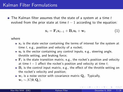
The Kalman filter assumes that the state of a system at a time tevolved from the prior state at time t− 1 according to the equation:
xt = Ftxt−1 +Btut +wt (1)
where
xt is the state vector containing the terms of interest for the system attime t, e.g., position and velocity of a rocket;ut is the vector containing any control inputs, e.g., steering angle,throttle setting, and braking force;Ft is the state transition matrix, e.g., the rocket’s position and velocityat time t− 1 affect the rocket’s position and velocity at time t;Bt is the control input matrix, e.g., the effect of the throttle setting onthe rocket’s velocity and position;wt is a noise vector with covariance matrix Qt. Typically,wt ∼ N (0,Qt).
Man-Wai MAK (EIE) Kalman Filter December 6, 2020 7 / 25
Kalman Filter Formulations
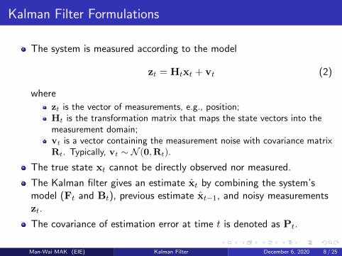
The system is measured according to the model
zt = Htxt + vt (2)
where
zt is the vector of measurements, e.g., position;Ht is the transformation matrix that maps the state vectors into themeasurement domain;vt is a vector containing the measurement noise with covariance matrixRt. Typically, vt ∼ N (0,Rt).
The true state xt cannot be directly observed nor measured.
The Kalman filter gives an estimate x̂t by combining the system’smodel (Ft and Bt), previous estimate x̂t−1, and noisy measurementszt.
The covariance of estimation error at time t is denoted as Pt.
Man-Wai MAK (EIE) Kalman Filter December 6, 2020 8 / 25
Kalman Filter Formulations
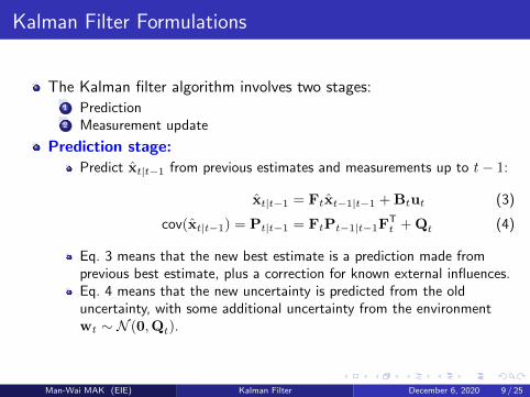
The Kalman filter algorithm involves two stages:1 Prediction2 Measurement update
Prediction stage:Predict x̂t|t−1 from previous estimates and measurements up to t− 1:
x̂t|t−1 = Ftx̂t−1|t−1 +Btut (3)
cov(x̂t|t−1) = Pt|t−1 = FtPt−1|t−1FTt +Qt (4)
Eq. 3 means that the new best estimate is a prediction made fromprevious best estimate, plus a correction for known external influences.Eq. 4 means that the new uncertainty is predicted from the olduncertainty, with some additional uncertainty from the environmentwt ∼ N (0,Qt).
Man-Wai MAK (EIE) Kalman Filter December 6, 2020 9 / 25
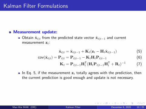
Kalman Filter Formulations
Measurement update:Obtain x̂t|t from the predicted state vector x̂t|t−1 and currentmeasurement zt:
x̂t|t = x̂t|t−1 +Kt(zt −Htx̂t|t−1) (5)
cov(x̂t|t) = Pt|t = Pt|t−1 −KtHtPt|t−1 (6)
Kt = Pt|t−1HTt (HtPt|t−1H
Tt +Rt)
−1 (7)
In Eq. 5, if the measurement zt totally agrees with the prediction, thenthe current prediction is good enough and update is not necessary.
Man-Wai MAK (EIE) Kalman Filter December 6, 2020 10 / 25
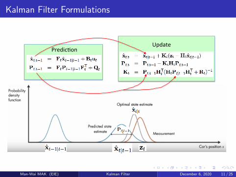
Kalman Filter Formulations
Predic'onUpdate
Man-Wai MAK (EIE) Kalman Filter December 6, 2020 11 / 25
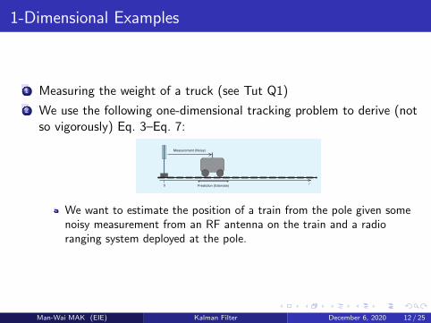
1-Dimensional Examples
1 Measuring the weight of a truck (see Tut Q1)
2 We use the following one-dimensional tracking problem to derive (notso vigorously) Eq. 3–Eq. 7:
IEEE SIGNAL PROCESSING MAGAZINE [129] SEPTEMBER 2012
control input parameter in the vector ut on the state vector (e.g., applies the effect of the throttle set-ting on the system velocity and position)
■ wt is the vector containing the process noise terms for each parame-ter in the state vector. The process noise is assumed to be drawn from a zero mean multivariate normal distribution with covariance given by the covariance matrix Qt.
Measurements of the system can also be performed, according to the model
H x vzt t t t= + , (2)
where ■ zt is the vector of measurements ■ Ht is the transformation matrix
that maps the state vector parame-ters into the measurement domain
■ vt is the vector containing the measurement noise terms for each observation in the measurement vec-tor. Like the process noise, the mea-surement noise is assumed to be zero mean Gaussian white noise with covariance Rt.
In the derivation that follows, we will consider a simple one-dimensional track-ing problem, particularly that of a train moving along a railway line (see Figure 1). We can therefore consider some example vectors and matrices in this problem. The state vector xt contains the position and velocity of the train
xxxt
t
t=
o; E.
The train driver may apply a braking or accelerating input to the system, which
we will consider here as a function of an applied force ft and the mass of the train m. Such control information is stored within the control vector ut
umf
tt= .
The relationship between the force applied via the brake or throttle during the time period ∆t (the time elapsed between time epochs t-1 and t) and the position and velocity of the train is given by the following equations:
( )( )x x x t
mf t
2t t tt
1 1
2
# TT
= + +- -o
x xm
f tt t
t1
T= +-o o .
These linear equations can be written in matrix form as
( )xx
t xx
t
tmf1
0 1 2t
t
t
t
t1
1
2T
T
T= +
-
-o o; ; ;
>E E E
H.
And so by comparison with (1), we can see for this example that
tT
F B ( )t t10 1
andt t
2T T= =
2;
>E
H .
The true state of the system xt cannot be directly observed, and the Kalman filter provides an algorithm to determine an estimate xtt by combining models of the system and noisy measurements of cer-tain parameters or linear functions of parameters. The estimates of the param-eters of interest in the state vector are therefore now provided by probability density functions (pdfs), rather than dis-crete values. The Kalman filter is based on Gaussian pdfs, as will become clear
following the derivation outlined below in the “Solutions” section. To fully describe the Gaussian functions, we need to know their variances and covari-ances, and these are stored in the covari-ance matrix Pt. The terms along the main diagonal of Pt are the variances associated with the corresponding terms in the state vector. The off-diagonal terms of Pt provide the covariances between terms in the state vector. In the case of a well-modeled, one-dimensional linear system with measurement errors drawn from a zero-mean Gaussian distri-bution, the Kalman filter has been shown to be the optimal estimator [1]. In the remainder of this article, we will derive the Kalman filter equations that allow us to recursively calculate xtt by combining prior knowledge, predictions from systems models, and noisy mea-surements.
The Kalman filter algorithm involves two stages: prediction and measure-ment update. The standard Kalman fil-ter equations for the prediction stage are
x F x B ut t t t t t t1 1 1= +; ;- - -t t (3)
P F P F Qt t t t t t t1 1 1T= +; ;- - - , (4)
where Qt is the process noise covariance matrix associated with noisy control inputs. Equation (3) was derived explic-itly in the discussion above. We can derive (4) as follows. The variance asso-ciated with the prediction xt t 1; -t of an unknown true value xt is given by
[( ) ( ) ]P x x x xE ,t t t t t t t tT
1 1 1= - -; ; ;- - -t t
and taking the difference between (3) and (1) gives
Prediction (Estimate)
Measurement (Noisy)
0 r
[FIG1] This figure shows the one-dim ensional system under consideration.
We want to estimate the position of a train from the pole given somenoisy measurement from an RF antenna on the train and a radioranging system deployed at the pole.
Man-Wai MAK (EIE) Kalman Filter December 6, 2020 12 / 25
1-Dimensional Examples
xt: The unknown (hidden state) distance from the pole to the train’sposition at time t;
zt: Noisy measure of the distance between the pole and the train’s RFantenna at time t using time-of-flight techniques;
H: A proportional scale to make the time-of-flight measurementcompatible with that of distance xt;
ut: The amount of throttle or brake applied by the train’s operator attime t;
B: A proportional scale to convert ut into distance;
wt: Noise of xt;
vt: Measurement noise.
Man-Wai MAK (EIE) Kalman Filter December 6, 2020 13 / 25
1-Dimensional Examples
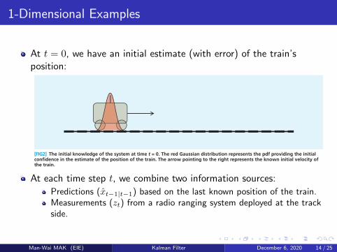
At t = 0, we have an initial estimate (with error) of the train’sposition:
IEEE SIGNAL PROCESSING MAGAZINE [130] SEPTEMBER 2012
[lecture NOTES] continued
( )x x F x x wt t t t t t t1 1 1- = - +; ;- - -t t
[( ( )
) ( ( )
) ]
P F x x
F x x
E
w
w
t t t t t
t t t t
tT
1 1 1 1
1 1 1
&
#
= -
+ -
+
; ;
;
- - - -
- - -
t
t
[( )
( ) ]
[(
) ]
[
]
[ ] .
F x x
x x
F F x
x w
w x
x F
w w
E
E
E
E
t t t
t t t
t
t t t
t t
t t
t t
1 1 1
1 1 1
1
1 1
1
1 1
T
T
T
T T
T
#
#
= -
-
+
-
+
-
+
;
;
;
;
- - -
- - -
-
- -
-
- -
t
t
t
t
Noting that the state estimation errors and process noise are uncorrelated
[( ) ]
( )
E x x w
E w x x 0t t t t
T
t t t tT
1 1 1
1 1 1
-
= - =
;
;
- - -
- - -
t
t6 @
[( ) (
) ] [ ]
.
P F x x x
x F w w
P FP F Q
E
Et t t t t t
t t t t
t t t t t
1 1 1 1 1
1 1
1 1 1
T T T
T
&
&
= -
- +
= +
; ;
;
; ;
- - - - -
- -
- - -
t
t
The measurement update equations are given by
x H x )(x K zt t tt t t t t t1 1= + -; ; ;- -t t t (5)
P P K H Pt t t t t t1 t t 1= -; ; - ; - , (6)
where
K P H H P H R( ) .T Tt t t t t t t t t1 1
1= +; ;- -- (7)
In the remainder of this article, we will derive the measurement update equa-tions [(5)–(7)] from first principles.
SOLUTIONSThe Kalman filter will be derived here by considering a simple one-dimension-al tracking problem, specifically that of a train is moving along a railway line. At every measurement epoch we wish to
know the best possible estimate of the location of the train (or more precisely, the location of the radio antenna mount-ed on the train roof). Information is avail-able from two sources: 1) predictions based on the last known position and velocity of the train and 2) measurements
from a radio ranging system deployed at the track side. The information from the predictions and measurements are com-bined to provide the best possible estimate of the location of the train. The system is shown graphically in Figure 1.
The initial state of the system (at time t = 0 s) is known to a reasonable accuracy, as shown in Figure 2. The location of the train is given by a Gaussian pdf. At the next time epoch ( )t 1 s= , we can estimate the new posi-tion of the train, based on known limita-tions such as its position and velocity at t = 0, its maximum possible acceleration and deceleration, etc. In practice, we may have some knowledge of the control inputs on the brake or accelerator by the driver. In any case, we have a prediction of the new position of the train, represented in Figure 3 by a new Gaussian pdf with a new mean and variance. Mathematically this step is represented by (1). The vari-ance has increased [see (2)], representing our reduced certainty in the accuracy of our position estimate compared to t = 0, due to the uncertainty associated with any process noise from accelerations or decel-erations undertaken from time t = 0 to time t = 1.
[FIG2] The initial knowledge of the system at time t = 0. The red Gaussian distribution represents the pdf providing the initial confidence in the estimate of the position of the train. The arrow pointing to the right represents the known initial velocity of the train.
??????Prediction (Estimate)
[FIG3] Here, the predict ion of the location of the train at time t = 1 and the level of uncertainty in that prediction is shown. The confidence in the knowledge of the position of the train has decreased, as we are not certain if the train has undergone any accelerations or decelerations in the intervening period from t = 0 to t = 1.
THE BEST ESTIMATE WE CAN MAKE OF THE
LOCATION OF THE TRAIN IS PROVIDED BY COMBINING OUR KNOWLEDGE FROM
THE PREDICTION AND THE MEASUREMENT.
At each time step t, we combine two information sources:
Predictions (x̂t−1|t−1) based on the last known position of the train.Measurements (zt) from a radio ranging system deployed at the trackside.
Man-Wai MAK (EIE) Kalman Filter December 6, 2020 14 / 25
1-Dimensional Examples
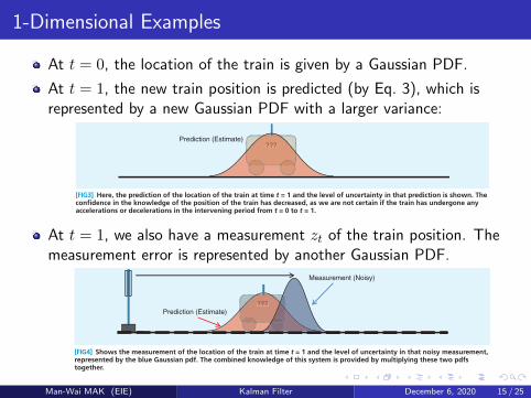
At t = 0, the location of the train is given by a Gaussian PDF.
At t = 1, the new train position is predicted (by Eq. 3), which isrepresented by a new Gaussian PDF with a larger variance:
IEEE SIGNAL PROCESSING MAGAZINE [130] SEPTEMBER 2012
[lecture NOTES] continued
( )x x F x x wt t t t t t t1 1 1- = - +; ;- - -t t
[( ( )
) ( ( )
) ]
P F x x
F x x
E
w
w
t t t t t
t t t t
tT
1 1 1 1
1 1 1
&
#
= -
+ -
+
; ;
;
- - - -
- - -
t
t
[( )
( ) ]
[(
) ]
[
]
[ ] .
F x x
x x
F F x
x w
w x
x F
w w
E
E
E
E
t t t
t t t
t
t t t
t t
t t
t t
1 1 1
1 1 1
1
1 1
1
1 1
T
T
T
T T
T
#
#
= -
-
+
-
+
-
+
;
;
;
;
- - -
- - -
-
- -
-
- -
t
t
t
t
Noting that the state estimation errors and process noise are uncorrelated
[( ) ]
( )
E x x w
E w x x 0t t t t
T
t t t tT
1 1 1
1 1 1
-
= - =
;
;
- - -
- - -
t
t6 @
[( ) (
) ] [ ]
.
P F x x x
x F w w
P FP F Q
E
Et t t t t t
t t t t
t t t t t
1 1 1 1 1
1 1
1 1 1
T T T
T
&
&
= -
- +
= +
; ;
;
; ;
- - - - -
- -
- - -
t
t
The measurement update equations are given by
x H x )(x K zt t tt t t t t t1 1= + -; ; ;- -t t t (5)
P P K H Pt t t t t t1 t t 1= -; ; - ; - , (6)
where
K P H H P H R( ) .T Tt t t t t t t t t1 1
1= +; ;- -- (7)
In the remainder of this article, we will derive the measurement update equa-tions [(5)–(7)] from first principles.
SOLUTIONSThe Kalman filter will be derived here by considering a simple one-dimension-al tracking problem, specifically that of a train is moving along a railway line. At every measurement epoch we wish to
know the best possible estimate of the location of the train (or more precisely, the location of the radio antenna mount-ed on the train roof). Information is avail-able from two sources: 1) predictions based on the last known position and velocity of the train and 2) measurements
from a radio ranging system deployed at the track side. The information from the predictions and measurements are com-bined to provide the best possible estimate of the location of the train. The system is shown graphically in Figure 1.
The initial state of the system (at time t = 0 s) is known to a reasonable accuracy, as shown in Figure 2. The location of the train is given by a Gaussian pdf. At the next time epoch ( )t 1 s= , we can estimate the new posi-tion of the train, based on known limita-tions such as its position and velocity at t = 0, its maximum possible acceleration and deceleration, etc. In practice, we may have some knowledge of the control inputs on the brake or accelerator by the driver. In any case, we have a prediction of the new position of the train, represented in Figure 3 by a new Gaussian pdf with a new mean and variance. Mathematically this step is represented by (1). The vari-ance has increased [see (2)], representing our reduced certainty in the accuracy of our position estimate compared to t = 0, due to the uncertainty associated with any process noise from accelerations or decel-erations undertaken from time t = 0 to time t = 1.
[FIG2] The initial knowledge of the system at time t = 0. The red Gaussian distribution represents the pdf providing the initial confidence in the estimate of the position of the train. The arrow pointing to the right represents the known initial velocity of the train.
??????Prediction (Estimate)
[FIG3] Here, the predict ion of the location of the train at time t = 1 and the level of uncertainty in that prediction is shown. The confidence in the knowledge of the position of the train has decreased, as we are not certain if the train has undergone any accelerations or decelerations in the intervening period from t = 0 to t = 1.
THE BEST ESTIMATE WE CAN MAKE OF THE
LOCATION OF THE TRAIN IS PROVIDED BY COMBINING OUR KNOWLEDGE FROM
THE PREDICTION AND THE MEASUREMENT.
At t = 1, we also have a measurement zt of the train position. Themeasurement error is represented by another Gaussian PDF.
IEEE SIGNAL PROCESSING MAGAZINE [131] SEPTEMBER 2012
At t = 1, we also make a measure-ment of the location of the train using the radio positioning system, and this is represented by the blue Gaussian pdf in Figure 4. The best estimate we can make of the location of the train is provided by combining our knowledge from the pre-diction and the measurement. This is achieved by multiplying the two corre-sponding pdfs together. This is repre-sented by the green pdf in Figure 5.
A key property of the Gaussian function is exploited at this point: the product of two Gaussian functions is another Gaussian function. This is critical as it permits an endless number of Gaussian pdfs to be multiplied over time, but the resulting function does not increase in complexity or number of terms; after each time epoch the new pdf is fully represented by a Gaussian function. This is the key to the elegant recursive properties of the Kalman filter.
The stages described above in the fig-ures are now considered again mathe-matically to derive the Kalman filter measurement update equations.
The prediction pdf represented by the red Gaussian function in Figure 3 is given by the equation
( )y r e2
1; ,( )r
1 1 112 2 1
21
2
_
rn v
vv
n-
-
. (8)
The measurement pdf represented by the blue Gaussian function in Figure 4 is given by
( )y r e2
1; ,( )r
2 2 222 2 2
22
2
_vr
nv
v
n-
-
. (9)
The information provided by these two pdfs is fused by multiplying the two together, i.e., considering the prediction and the measurement together (see Figure 5). The new pdf representing the fusion of the
information from the prediction and mea-surement, and our best current estimate of the system, is therefore given by the prod-uct of these two Gaussian functions
( , )
.
y r
e
,
21
21
21
; ,( ) ( )
( (
r r
r r
1 1 2 2
12 2
22 2
12
22 2 2
fused
) )
121
2
222
2
121
2222 2
r r
r
n v n v
v v
v v=
v
n
v
n
v
n
v
n
--
--
--
+-
e e#=
e o
(10)
The quadratic terms in this new function can expanded and then the whole expression rewritten in Gaussian form
( )r n-
( )
2
y r
1
; ,
2 2
fused fused fused
fused
2
2
fused
fused
r
n v
vv
-e= , (11)
where
( )
12
22
1 22
2 12
112
22
12
2 1
fusednv v
n v n v
nv v
v n n
=+
+
= ++
-
(12)
and
2
12
22
12
22
12
12
22
14
fusedvv v
v vv
v v
v=
+= -
+.
(13)
These last two equations represent the measurement update steps of the Kalman filter algorithm, as will be shown explicitly below. However, to present a more general case, we need to consider an extension to this example.
In the example above, it was assumed that the predictions and measurements were made in the same coordinate frame and in the same units. This has resulted in a particularly concise pair of
??????
Measurement (Noisy)
Prediction (Estimate)
[FIG4] Shows the measur ement of the location of the train at time t = 1 and the level of uncertainty in that noisy measurement, represented by the blue Gaussian pdf. The combined knowledge of this system is provided by multiplying these two pdfs together.
???
Measurement (Noisy)
Prediction (Estimate)
[FIG5] Shows the new pdf (green) generated by multiplying the pdfs associated with the prediction and measurement of the train’s location at time t = 1. This new pdf provides the best estimate of the location of the train, by fusing the data from the prediction and the measurement.
A KEY PROPERTY OF THE GAUSSIAN FUNCTION IS
EXPLOITED AT THIS POINT: THE PRODUCT OF TWO GAUSSIAN FUNCTIONS IS ANOTHER GAUSSIAN
FUNCTION.
Man-Wai MAK (EIE) Kalman Filter December 6, 2020 15 / 25
1-Dimensional Examples
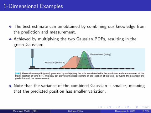
The best estimate can be obtained by combining our knowledge fromthe prediction and measurement.
Achieved by multiplying the two Gaussian PDFs, resulting in thegreen Gaussian:
IEEE SIGNAL PROCESSING MAGAZINE [131] SEPTEMBER 2012
At t = 1, we also make a measure-ment of the location of the train using the radio positioning system, and this is represented by the blue Gaussian pdf in Figure 4. The best estimate we can make of the location of the train is provided by combining our knowledge from the pre-diction and the measurement. This is achieved by multiplying the two corre-sponding pdfs together. This is repre-sented by the green pdf in Figure 5.
A key property of the Gaussian function is exploited at this point: the product of two Gaussian functions is another Gaussian function. This is critical as it permits an endless number of Gaussian pdfs to be multiplied over time, but the resulting function does not increase in complexity or number of terms; after each time epoch the new pdf is fully represented by a Gaussian function. This is the key to the elegant recursive properties of the Kalman filter.
The stages described above in the fig-ures are now considered again mathe-matically to derive the Kalman filter measurement update equations.
The prediction pdf represented by the red Gaussian function in Figure 3 is given by the equation
( )y r e2
1; ,( )r
1 1 112 2 1
21
2
_
rn v
vv
n-
-
. (8)
The measurement pdf represented by the blue Gaussian function in Figure 4 is given by
( )y r e2
1; ,( )r
2 2 222 2 2
22
2
_vr
nv
v
n-
-
. (9)
The information provided by these two pdfs is fused by multiplying the two together, i.e., considering the prediction and the measurement together (see Figure 5). The new pdf representing the fusion of the
information from the prediction and mea-surement, and our best current estimate of the system, is therefore given by the prod-uct of these two Gaussian functions
( , )
.
y r
e
,
21
21
21
; ,( ) ( )
( (
r r
r r
1 1 2 2
12 2
22 2
12
22 2 2
fused
) )
121
2
222
2
121
2222 2
r r
r
n v n v
v v
v v=
v
n
v
n
v
n
v
n
--
--
--
+-
e e#=
e o
(10)
The quadratic terms in this new function can expanded and then the whole expression rewritten in Gaussian form
( )r n-
( )
2
y r
1
; ,
2 2
fused fused fused
fused
2
2
fused
fused
r
n v
vv
-e= , (11)
where
( )
12
22
1 22
2 12
112
22
12
2 1
fusednv v
n v n v
nv v
v n n
=+
+
= ++
-
(12)
and
2
12
22
12
22
12
12
22
14
fusedvv v
v vv
v v
v=
+= -
+.
(13)
These last two equations represent the measurement update steps of the Kalman filter algorithm, as will be shown explicitly below. However, to present a more general case, we need to consider an extension to this example.
In the example above, it was assumed that the predictions and measurements were made in the same coordinate frame and in the same units. This has resulted in a particularly concise pair of
??????
Measurement (Noisy)
Prediction (Estimate)
[FIG4] Shows the measur ement of the location of the train at time t = 1 and the level of uncertainty in that noisy measurement, represented by the blue Gaussian pdf. The combined knowledge of this system is provided by multiplying these two pdfs together.
???
Measurement (Noisy)
Prediction (Estimate)
[FIG5] Shows the new pdf (green) generated by multiplying the pdfs associated with the prediction and measurement of the train’s location at time t = 1. This new pdf provides the best estimate of the location of the train, by fusing the data from the prediction and the measurement.
A KEY PROPERTY OF THE GAUSSIAN FUNCTION IS
EXPLOITED AT THIS POINT: THE PRODUCT OF TWO GAUSSIAN FUNCTIONS IS ANOTHER GAUSSIAN
FUNCTION.
Note that the variance of the combined Gaussian is smaller, meaningthat the predicted position has smaller variation.
Man-Wai MAK (EIE) Kalman Filter December 6, 2020 16 / 25
1-Dimensional Examples
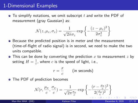
To simplify notations, we omit subscript t and write the PDF ofmeasurement (gray Gaussian) as:
N (z, µz, σz) =1√2πσz
exp
{−(z − µz)2
2σ2z
}Because the predicted position is in meter and the measurement(time-of-flight of radio signal) is in second, we need to make the twounits compatible.
This can be done by converting the prediction x to measurement z bysetting H = 1
c , where c is the speed of light, i.e.,
r =x
c(in seconds)
The PDF of prediction becomes
N (r,µxc,σxc) =
1√2π σxc
exp
{−(r − µx
c )2
2(σxc )2
}Man-Wai MAK (EIE) Kalman Filter December 6, 2020 17 / 25
1-Dimensional Examples
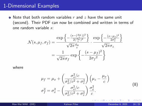
Note that both random variables r and z have the same unit(second). Their PDF can now be combined and written in terms ofone random variable s:
N (s, µf , σf ) =exp
{− (s−(µx
c))2
2(σxc)2
}√2π σxc
·exp
{− (s−µz)2
2σ2z
}√2πσz
=1√2πσf
exp
{−(s− µf )2
2σf 2
}where
µf = µx +
(σ2x/c
σ2x/c2 + σ2z
)(µz −
µxc
)σ2f = σ2x −
(σ2x/c
σ2x/c2 + σ2z
)σ2xc.
(8)
Man-Wai MAK (EIE) Kalman Filter December 6, 2020 18 / 25
1-Dimensional Examples
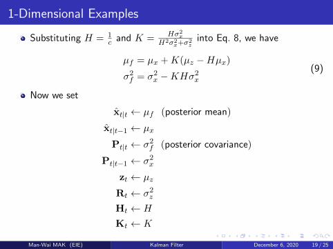
Substituting H = 1c and K = Hσ2
xH2σ2
x+σ2z
into Eq. 8, we have
µf = µx +K(µz −Hµx)σ2f = σ2x −KHσ2x
(9)
Now we set
x̂t|t ← µf (posterior mean)
x̂t|t−1 ← µx
Pt|t ← σ2f (posterior covariance)
Pt|t−1 ← σ2x
zt ← µz
Rt ← σ2z
Ht ← H
Kt ← K
Man-Wai MAK (EIE) Kalman Filter December 6, 2020 19 / 25
1-Dimensional Examples
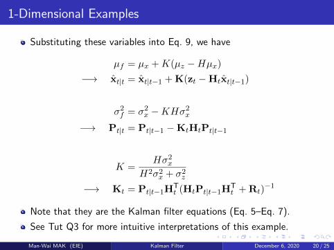
Substituting these variables into Eq. 9, we have
µf = µx +K(µz −Hµx)−→ x̂t|t = x̂t|t−1 +K(zt −Htx̂t|t−1)
σ2f = σ2x −KHσ2x−→ Pt|t = Pt|t−1 −KtHtPt|t−1
K =Hσ2x
H2σ2x + σ2z
−→ Kt = Pt|t−1HTt (HtPt|t−1H
Tt +Rt)
−1
Note that they are the Kalman filter equations (Eq. 5–Eq. 7).
See Tut Q3 for more intuitive interpretations of this example.
Man-Wai MAK (EIE) Kalman Filter December 6, 2020 20 / 25
1-Dimensional Examples
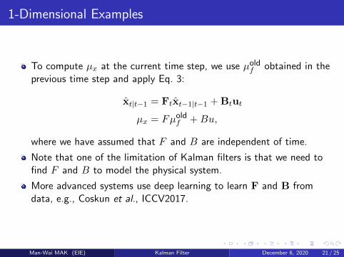
To compute µx at the current time step, we use µoldf obtained in theprevious time step and apply Eq. 3:
x̂t|t−1 = Ftx̂t−1|t−1 +Btut
µx = Fµoldf +Bu,
where we have assumed that F and B are independent of time.
Note that one of the limitation of Kalman filters is that we need tofind F and B to model the physical system.
More advanced systems use deep learning to learn F and B fromdata, e.g., Coskun et al., ICCV2017.
Man-Wai MAK (EIE) Kalman Filter December 6, 2020 21 / 25

End of Notes
Man-Wai MAK (EIE) Kalman Filter December 6, 2020 22 / 25
Kalman Filter Formulations (Optional)
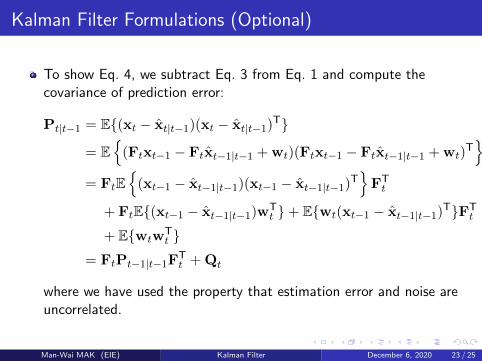
To show Eq. 4, we subtract Eq. 3 from Eq. 1 and compute thecovariance of prediction error:
Pt|t−1 = E{(xt − x̂t|t−1)(xt − x̂t|t−1)T}
= E{(Ftxt−1 − Ftx̂t−1|t−1 +wt)(Ftxt−1 − Ftx̂t−1|t−1 +wt)
T}
= FtE{(xt−1 − x̂t−1|t−1)(xt−1 − x̂t−1|t−1)
T}FTt
+ FtE{(xt−1 − x̂t−1|t−1)wTt }+ E{wt(xt−1 − x̂t−1|t−1)
T}FTt
+ E{wtwTt }
= FtPt−1|t−1FTt +Qt
where we have used the property that estimation error and noise areuncorrelated.
Man-Wai MAK (EIE) Kalman Filter December 6, 2020 23 / 25
Kalman Filter Formulations (Optional)
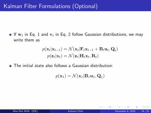
If wt in Eq. 1 and vt in Eq. 2 follow Gaussian distributions, we maywrite them as
p(xt|xt−1) = N (xt|Ftxt−1 +Btut,Qt)
p(zt|xt) = N (zt|Htxt,Rt)
The initial state also follows a Gaussian distribution:
p(x1) = N (x1|B1u1,Q1)
Man-Wai MAK (EIE) Kalman Filter December 6, 2020 24 / 25
Kalman Filter’s Output and Optimal Linear Estimate(Optional)
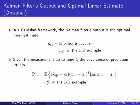
In a Gaussian framework, the Kalman filter’s output is the optimallinear estimate:
x̂t|t = E{xt|z0, z1, . . . , zt}= µf,t in the 1-D example
Given the measurement up to time t, the covariance of predictionerror is
Pt|t = E{(x̂t|t − xt)(x̂t|t − xt)
T|z0, z1, . . . , zt}
= σ2f,t in the 1-D example
Man-Wai MAK (EIE) Kalman Filter December 6, 2020 25 / 25