a kalman filter for active feedback on rotating external kink
TRANSCRIPT

A Kalman Filter for Active Feedback on
Rotating External Kink Instabilities in a
Tokamak Plasma
Jeremy Mark Hanson
SUBMITTED IN PARTIAL FULFILLMENT OF THE
REQUIREMENTS FOR THE DEGREE
OF DOCTOR OF PHILOSOPHY
IN THE GRADUATE SCHOOL OF ARTS AND SCIENCES
Columbia University
2009

c 2009
Jeremy Mark Hanson
All Rights Reserved
ABSTRACT
A Kalman Filter for Active Feedback on Rotating External Kink Instabilities in a
Tokamak Plasma
Jeremy M. Hanson
The first experimental demonstration of feedback suppression of rotating external
kink modes near the ideal wall limit in a tokamak using Kalman filtering to discrimi-
nate the 𝑛 = 1 kink mode from background noise is reported. In order to achieve the
highest plasma pressure limits in tokamak fusion experiments, feedback stabilization
of long-wavelength, external instabilities will be required, and feedback algorithms will
need to distinguish the unstable mode from noise due to other magnetohydrodynamic
activity. When noise is present in measurements of a system, a Kalman filter can be
used to compare the measurements with an internal model, producing a realtime, op-
timal estimate for the system’s state. For the work described here, the Kalman filter
contains an internal model that captures the dynamics of a rotating, growing instabil-
ity and produces an estimate for the instability’s amplitude and spatial phase. On the
High Beta Tokamak-Extended Pulse (HBT-EP) experiment, the Kalman filter algo-
rithm is implemented using a set of digital, field-programmable gate array controllers
with 10 microsecond latencies. The feedback system with the Kalman filter is able to
suppress the external kink mode over a broad range of spatial phase angles between
the sensed mode and applied control field, and performance is robust at noise levels
that render feedback with a classical, proportional gain algorithm ineffective. Scans
of filter parameters show good agreement between simulation and experiment, and
feedback suppression and excitation of the kink mode are enhanced in experiments
when a filter made using optimal parameters from the experimental scans is used.
Contents
1 Introduction 1
1.1 Nuclear Fusion . . . . . . . . . . . . . . . . . . . . . . . . . . . . . . 1
1.2 Tokamaks and their stability limits . . . . . . . . . . . . . . . . . . . 3
1.3 Feedback control of resistive wall modes . . . . . . . . . . . . . . . . 6
1.4 The HBT-EP experiment . . . . . . . . . . . . . . . . . . . . . . . . . 8
1.5 Principal results . . . . . . . . . . . . . . . . . . . . . . . . . . . . . . 10
1.6 Outline of this Thesis . . . . . . . . . . . . . . . . . . . . . . . . . . . 11
2 Physics of the tokamak external kink mode 16
2.1 Ideal magnetohydrodynamics . . . . . . . . . . . . . . . . . . . . . . 17
2.2 Ideal MHD equilibrium . . . . . . . . . . . . . . . . . . . . . . . . . . 19
2.3 Stability of ideal MHD equilibria . . . . . . . . . . . . . . . . . . . . 20
2.4 The ideal, external kink mode . . . . . . . . . . . . . . . . . . . . . . 23
2.5 The resistive wall mode . . . . . . . . . . . . . . . . . . . . . . . . . . 25
3 Simulating external kink mode feedback 29
3.1 Models for the resistive wall mode . . . . . . . . . . . . . . . . . . . . 29
3.2 The reduced Fitzpatrick–Aydemir equations . . . . . . . . . . . . . . 31
3.3 Simulating feedback and noise . . . . . . . . . . . . . . . . . . . . . . 33
i

3.4 Example simulation results . . . . . . . . . . . . . . . . . . . . . . . . 35
4 The Kalman filter 38
4.1 The linear control problem . . . . . . . . . . . . . . . . . . . . . . . . 39
4.2 Linear observers . . . . . . . . . . . . . . . . . . . . . . . . . . . . . . 41
4.3 The Kalman filter . . . . . . . . . . . . . . . . . . . . . . . . . . . . . 42
4.4 Filter matrices for external kink mode control . . . . . . . . . . . . . 46
4.5 Feedback simulations with the Kalman filter . . . . . . . . . . . . . . 50
5 Control system hardware on HBT-EP 53
5.1 Adjustable wall sections . . . . . . . . . . . . . . . . . . . . . . . . . 53
5.2 Feedback loop hardware . . . . . . . . . . . . . . . . . . . . . . . . . 55
5.3 Feedback algorithm . . . . . . . . . . . . . . . . . . . . . . . . . . . . 59
6 Observation of external kink mode activity 64
6.1 Discharge programming . . . . . . . . . . . . . . . . . . . . . . . . . 64
6.2 Analysis of magnetic fluctuations . . . . . . . . . . . . . . . . . . . . 68
6.2.1 Fourier analysis . . . . . . . . . . . . . . . . . . . . . . . . . . 68
6.2.2 Biorthogonal decomposition analysis . . . . . . . . . . . . . . 70
7 Closed loop Kalman filter experiments 76
7.1 Experimental method . . . . . . . . . . . . . . . . . . . . . . . . . . . 77
7.2 Initial phase angle scan . . . . . . . . . . . . . . . . . . . . . . . . . . 79
7.3 Added noise experiments . . . . . . . . . . . . . . . . . . . . . . . . . 82
7.4 Optimization of Kalman filter parameters . . . . . . . . . . . . . . . . 84
7.5 Phase scan with optimized Kalman filter . . . . . . . . . . . . . . . . 88
ii

8 Conclusions and future work 91
8.1 Conclusions . . . . . . . . . . . . . . . . . . . . . . . . . . . . . . . . 91
8.2 Future work . . . . . . . . . . . . . . . . . . . . . . . . . . . . . . . . 94
Appendices 97
A FPGA programming considerations 97
B Feedback algorithm 100
B.1 Equations solved . . . . . . . . . . . . . . . . . . . . . . . . . . . . . 100
B.2 Description of the algorithm . . . . . . . . . . . . . . . . . . . . . . . 103
iii

List of Figures
1.1 Trajectories of cations and electrons in a constant magnetic field . . 3
1.2 A cutaway schematic of a tokamak showing vertical field (VF), Ohmic
heating (OH), and toroidal field (TF) coils, vacuum chamber, and
plasma. The OH solenoid is used to drive a plasma current in the
toroidal direction, 𝜙. The plasma current produces a magnetic field in
the poloidal direction, 𝜃. . . . . . . . . . . . . . . . . . . . . . . . . . 4
1.3 A photo of the HBT-EP experiment showing toroidal and vertical field
magnets and the vacuum vessel. . . . . . . . . . . . . . . . . . . . . . 8
1.4 The arrangement of the stainless steel and aluminum wall sections in
the HBT-EP experiment. . . . . . . . . . . . . . . . . . . . . . . . . . 10
2.1 Cross-sectional sketches of tokamak equilibrium quantities at low 𝛽: a)
circular flux surfaces, b) poloidal and vacuum toroidal magnetic field
profiles, and c) current density and safety factor profiles. . . . . . . . 19
2.2 A magnetic field line with a 𝑚/𝑛 = 3/1 helicity makes three toroidal
transits for every poloidal transit. . . . . . . . . . . . . . . . . . . . . 20
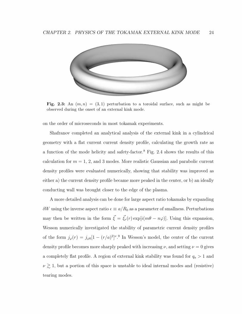
2.3 An (𝑚,𝑛) = (3, 1) perturbation to a toroidal surface, such as might be
observed during the onset of an external kink mode. . . . . . . . . . . 24
iv

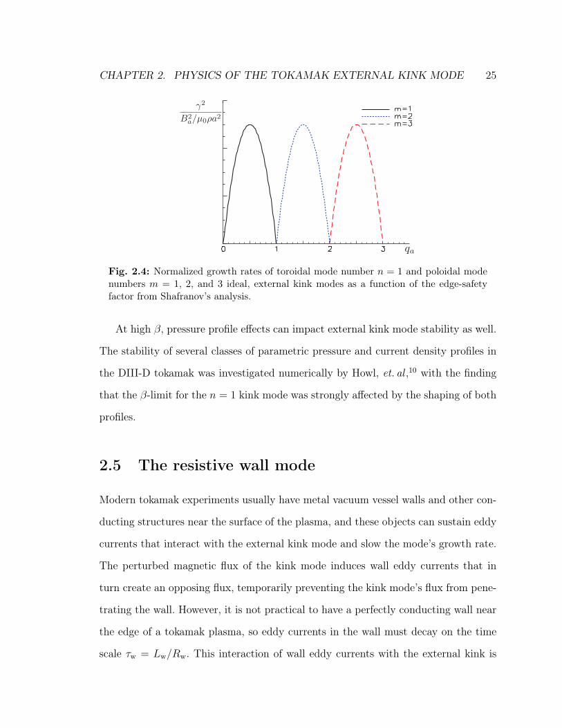
2.4 Normalized growth rates of toroidal mode number 𝑛 = 1 and poloidal
mode numbers 𝑚 = 1, 2, and 3 ideal, external kink modes as a function
of the edge-safety factor from Shafranov’s analysis. . . . . . . . . . . 25
3.1 A stability diagram for Eq. 3.1 with 𝜓c = 0. The “+” symbol marks
the values 𝑠 = 1.0 and = −1.41 used the simulation. . . . . . . . . . 33
3.2 Control power and sine poloidal field measurements from feedback sim-
ulations with the reduced Fitzpatrick–Aydemir equations for cases with
a) no added noise, and b) Gaussian noise added to poloidal field mea-
surements. In the poloidal field measurements for part b), the black
trace shows the measurements without added noise. The measurements
with added noise (blue) are used to compute the feedback signal. . . . 36
4.1 The cosine and sine components of a growing, rotating mode. . . . . . 48
4.2 Control power and sine poloidal field measurements from feedback
simulations with the reduced Fitzpatrick–Aydemir equations for cases
without (a) and with (b) a Kalman observer. In part (a), the poloidal
field measurements with added noise (blue) are used to compute the
feedback signal. In part (b), the poloidal field measurements with added
noise are an input for the Kalman filter. The Kalman filter’s output
(red) is used to compute the control signal. In both parts, the poloidal
field without added noise is overlaid in black. . . . . . . . . . . . . . . 50
5.1 The approximate locations of the wall sections and feedback system
coils during external kink mode experiments are shown above. . . . . 54
v

5.2 The arrangement of the control and sensor coils in the 𝜙–𝜃 plane is
shown above. The coils are divided into four independent feedback
loops (groups a–d), with five sensor coils and five control coil pairs each. 56
5.3 A diagram of one out of four feedback loops. Signals from five sensor
coils are filtered using analog components before reaching the field-
programmable gate array (FPGA) controller. The outputs of the FPGA
are sent to amplifiers that drive five control coil pairs. . . . . . . . . . 57
5.4 Aggregate frequency-dependent amplitude and phase transfer func-
tions for all components in the feedback loop. The red, dashed lines
show the uncorrected transfer function. Solid, blue lines show the trans-
fer function when corrected by the phase-lag and phase-lead temporal
filters in the feedback algorithm.5 . . . . . . . . . . . . . . . . . . . . 58
5.5 A diagram showing the stages of the feedback algorithm. The 𝑛 =
1 mode is computed from a group of five sensor coils using a DFT
and optionally mixed with a noise input. The phase-lag, Kalman, and
phase-lead filters are then applied, followed by the proportional gain,
toroidal rotation, and inverse DFT operators. . . . . . . . . . . . . . 61
5.6 Example input and output signals from the feedback algorithm. a)
an input signal from a sensor coil for HBT-EP discharge 62335. b)
an output of an algorithm employing only the spatial and temporal
filtering. c) an output of the Kalman filter algorithm. . . . . . . . . . 62
6.1 Time evolutions of (a) the vertical field coil current, (b) the Ohmic
heating coil current, and (c) the toroidal field measured by a pickup
coil located at major radius 𝑅 = 123 cm for HBT-EP shot number
62112. . . . . . . . . . . . . . . . . . . . . . . . . . . . . . . . . . . . 65
vi

6.2 Time evolutions of the (a) plasma current, (b) plasma major radius, (c)
plasma minor radius, and (d) edge safety factor for HBT-EP discharge
62112. . . . . . . . . . . . . . . . . . . . . . . . . . . . . . . . . . . . 66
6.3 Time evolution (a) and frequency spectrum amplitude (b) of poloidal
field fluctuations measured by a feedback system sensor coil. The fre-
quency spectrum is computed over the highlighted time-window, 1.8–
2.8 msec. . . . . . . . . . . . . . . . . . . . . . . . . . . . . . . . . . . 67
6.4 Spatial Fourier spectrum amplitudes calculated from poloidal field sen-
sor fluctuations for HBT-EP discharge 62112. The colors denote poloidal
groupings of five sensors each. The highlighted region marks the time
window when 𝑞𝑎 < 3. . . . . . . . . . . . . . . . . . . . . . . . . . . . 69
6.5 Spatial Fourier spectrum phase for the 𝑛 = 1 mode for HBT-EP shot
62112. The colors of the traces denote individual sensor groups as in
Fig. 6.4. The highlighted region marks the time when 𝑞𝑎 < 3. . . . . . 70
6.6 Energy content of the mode spectrum obtained by applying the biorthog-
onal decomposition to poloidal field fluctuation data from HBT-EP
discharge 62112. . . . . . . . . . . . . . . . . . . . . . . . . . . . . . . 71
6.7 The first pair of spatial modes obtained using a biorthogonal decom-
position analysis of poloidal field fluctuations from HBT-EP discharge
62112. The peak amplitude of the modes is normalized to 1.0. . . . . 72
6.8 The second pair of spatial modes obtained using a biorthogonal decom-
position analysis of poloidal field fluctuations from HBT-EP discharge
62112. The peak amplitude of the modes is normalized to 1.0. . . . . 73
6.9 Time histories of the first four temporal modes obtained using a biorthog-
onal decomposition analysis of poloidal field fluctuations from HBT-EP
discharge 62112. . . . . . . . . . . . . . . . . . . . . . . . . . . . . . . 74vii
7.1 Shot-averaged time evolutions of the plasma current (a) and edge safety
factor (b) from 462 feedback-off discharges are shown in black. The gray
traces show the means plus and minus one standard deviation. . . . . 77
7.2 This diagram shows the toroidal dependence of the perturbed field of
an 𝑛 = 1 mode (dashed, red) overlaid with an 𝑛 = 1 feedback field
(solid, black). The spatial phasing between the mode and feedback,
∆𝜙f , is an adjustable control parameter. . . . . . . . . . . . . . . . . 79
7.3 Poloidal field fluctuations measured by a sensor coil 1 cm from the
plasma surface for the case of: (a) no feedback, (b) positive feedback
using the Kalman filter and (c) negative feedback with the Kalman filter. 80
7.4 The amplitude of the Fourier spectrum of poloidal field fluctuations
measured in HBT-EP during an initial scan of the feedback phase angle,
∆𝜙f . The radial axis marks the frequency of the Fourier spectrum, and
the polar axis marks the setting of ∆𝜙f . The peak of the feedback-off
frequency distribution occurs at 4 kHz and is marked on the color-bar.
The blue and red lines mark the locations of slices shown in Fig. 7.10-a. 81
7.5 Example signals from added noise experiments. Plot (a) shows a sim-
ulation of the 𝑛 = 1 cosine mode as calculated in the DFT step in
the algorithm (black) and the sum of this signal with the cosine com-
ponent of the added noise (gray). Plots (b) and (c) show one of five
FPGA outputs to the control coils in the added noise experiments for
algorithms with and without the Kalman filter, phased to excite the
mode. . . . . . . . . . . . . . . . . . . . . . . . . . . . . . . . . . . . 83
viii
7.6 A comparison of the Fourier spectrum amplitude of poloidal field fluc-
tuations for added noise experiments, for feedback off (solid, black),
Kalman filter feedback (dotted, red), and feedback without the Kalman
filter (dashed, blue). Plots (a) and (c) show suppression and excitation
experiments with no added noise. Plots (b) and (d) show the sup-
pression and excitation cases with extra noise added to the feedback
algorithms. . . . . . . . . . . . . . . . . . . . . . . . . . . . . . . . . 84
7.7 RMS-averaged poloidal field fluctuations from scans of the Kalman
filter model’s growth rate parameter 𝛾 in (a) simulation and (b) ex-
periment. The averages are expressed as percent differences from the
feedback-off RMS average. . . . . . . . . . . . . . . . . . . . . . . . . 85
7.8 RMS-averaged poloidal field fluctuations from scans of the Kalman
filter model’s rotation rate parameter 𝜔 in (a) simulation and (b) ex-
periment. The averages are expressed as percent differences from the
feedback-off RMS average. The scans were performed at two settings
for the diagonal terms in the Kalman filter’s plant noise covariance
matrix, 𝑄𝑖𝑖 = 1× 10⁻⁵ (diamonds), and 𝑄𝑖𝑖 = 1× 10⁻⁴ (stars). . . . . 86
7.9 The amplitude of the Fourier spectrum of poloidal field fluctuations
measured in HBT-EP during a scan of the feedback phase angle, ∆𝜙f ,
is shown above. This scan was done using the Kalman filter parameters
obtained from the optimization scans. The radial axis marks the fre-
quency of the Fourier spectrum, and the polar axis marks the setting
of ∆𝜙f . The peak of the feedback off frequency distribution occurs at
4 kHz and is marked on the color-bar. The blue and red lines mark the
locations of slices shown in Fig. 7.10-b. . . . . . . . . . . . . . . . . . 87
ix

7.10 Fourier spectrum amplitude of poloidal field fluctuations for cases of
feedback excitation (red, dashed), no feedback (black, solid), and feed-
back suppression (blue, dotted) from experiments (a) before and (b)
after optimization of Kalman filter parameters. . . . . . . . . . . . . . 88
7.11 A comparison of the Fourier spectrum amplitude of (a) (𝑚,𝑛) = (3, 1)
poloidal field fluctuations with (b) (𝑚,𝑛) = (6, 2) fluctuations from
the feedback phase angle scan with the optimized Kalman filter pa-
rameters. Note that the color-scales for parts (a) and (b) have different
ranges. . . . . . . . . . . . . . . . . . . . . . . . . . . . . . . . . . . . 89
8.1 Diagram of the planned first wall and feedback system upgrade for
HBT-EP. . . . . . . . . . . . . . . . . . . . . . . . . . . . . . . . . . . 95
B.1 A flow chart for the Kalman filter algorithm. . . . . . . . . . . . . . . 104
x

List of Tables
1.1 Device parameters for HBT-EP. . . . . . . . . . . . . . . . . . . . . . 9
3.1 Parameters used for simulations of the external kink mode. . . . . . . 35
xi

Acknowledgments
I started work on initial computer simulations for this thesis in the spring of 2006.
The road that brought me to the final experimental results, obtained during 2008, was
not an easy one to travel. I will avoid detailing my struggles here; I wish to instead
emphasize crucial support from numerous individuals I received throughout the course
of my work. Without this support, my progress would have been dramatically slower,
perhaps impossible.
I would first like to thank my advisors: Mike Mauel, Dave Maurer, Jerry Navratil,
Thomas Pedersen, and Amiya Sen. I have learned quite a bit about plasma physics
and feedback under your tutelage, and your patient comments and suggestions have
led to exciting discoveries. Your dedication and contagious enthusiasm have made it
a pleasure to work with you.
To HBT-EP’s dedicated technical staff: Jim Andrello, Moe Cea, and Nick Rivera,
your support has been essential in keeping the experiment operational. Thanks to
your knowledge and workmanship, I was able to make thousands of plasma discharges
during my years here. You also contribute greatly to the culture of the lab. I will miss
our long conversations.
No less important is the courteous assistance I received from the administrative
staff in the department of Applied Physics and Applied Mathematics. In particu-
lar, I would like to thank Dina Amin, Marlene Arbo, Montserrat Fernandez-Pinkley,xii

Michael Garcia, Ria Miranda, Christina Rohm, and Darya Shcherbanyuk.
To the other plasma physics graduate students, past and present, with whom I
have had the pleasure of sharing this journey: Bryan DeBono, Brian Grierson, Royce
James, Matt Lanctot, Jeff Levesque, Yuhong Liu, Oksana Katsuro-Hopkins, Alex
Klein, Dave Murphy, Daisuke Shiraki, and Matt Worstell, I have profited greatly
from our many conversations, and I wish you well in your continuing endeavors.
I wish to thank the staff at Stone Barns Center for Food and Agriculture for their
friendship and hospitality during the course of my work.
My parents, Mark and Anne, my brother, Joe and sister, Laura, and my family and
friends have provided constant encouragement and emotional support during these
years. Thank you for this. I miss you all greatly.
Finally, to my wife, Erika, you have been with me since the beginning of my
work here and supported my efforts in myriad ways. The plots and diagrams in this
thesis look splendid thanks to your instruction, advice, and criticism. Much more
importantly, you have stood by me through these difficult years with tenderness and
good humor. For this I am profoundly thankful.
xiii

ToErika
xiv

Chapter 1
Introduction
Many of the results presented in this Thesis have direct relevance to the development
of controlled nuclear fusion as an energy source. In this Chapter, the problem of
achieving sustainable fusion energy using magnetically confined plasmas is introduced.
Substantial progress toward this end has been made over the past five decades with
devices that confine the plasma in a toroidal geometry. One such device, the tokamak,
is the leading candidate for a fusion reactor. The viability of tokamak reactors is
limited by plasma instabilities, and the principal results of this Thesis apply to the
feedback control of one of the most restrictive tokamak instabilities, the ideal external
kink mode.
1.1 Nuclear Fusion
Nuclear fusion energy production, if it can be developed, will offer significant ad-
vantages over present-day fossil fuel and fission energy. Because very light atomic
nuclei, such as deuterium, tritium, and helium are involved in fusion, the problems
of long-term radioactive waste, catastrophic reactor failure, and proliferation of nu-
1

CHAPTER 1. INTRODUCTION 2
clear materials are much less severe compared with fission energy. Deuterium, one fuel
source for fusion, is abundant and easily accessible on earth. It is present in a con-
centration of 0.015 mol % in seawater, and it can be economically isolated.1 Finally,
fusion energy will not produce any greenhouse gasses or environmental pollutants, in
contrast with present-day fossil fuel energy sources.
In order for atomic nuclei to fuse, they must be made hot enough to overcome the
repulsive Coulomb force. A natural medium for achieving this condition is the plasma
state, and the sun provides evidence that a fusion reaction may indeed be sustained
this way: it is a gravitationally confined plasma that is undergoing a long-term fusion
“burn.” Lawson2 considered power balance requirements for a pulsed fusion reactor for
deuterium–deuterium (D–D) and deuterium–tritium (D–T) fusion reactions, taking
into account the power of the reactions themselves and losses due to bremsstrahlung
radiation, but ignoring any self-heating of the plasma.* For example, in a D–T reactor
with an energy-recycling efficiency of 30% and ion temperatures near 20 keV, the
product of the plasma number density 𝑛 and energy confinement time 𝜏 must satisfy
𝑛𝜏 > 3 × 10¹⁹ m−3s.3 Making a terrestrial fusion reactor that can satisfy Lawson’s
condition is an area of ongoing research.
It is impossible to create a gravitationally confined plasma on earth, and a plasma
cannot be confined by a solid container because contact with the walls of the container
causes the ions and electrons in the plasma to cool and recombine. However, plasmas
may be confined by magnetic fields. The Lorentz force causes charged particles to
move in helical paths around the magnetic field lines (see Fig. 1.1). In most successful
magnetic confinement devices, the plasma is trapped in a torus-shaped volume. The
toroidal geometry allows for the plasma to be confined on a nested set of surfaces of*The effect of heating from fusion 𝛼-particles can be trivially included in the derivation of the
Lawson criterion.

CHAPTER 1. INTRODUCTION 3
Fig. 1.1: Trajectories of cations and electrons in a constant magnetic field .
constant magnetic flux that do not intersect the vacuum vessel. The leading candidate
for a fusion reactor, the tokamak, is one such device.
1.2 Tokamaks and their stability limits
The announcement of record-breaking temperature, density, and confinement time
measurements from tokamak† devices in the mid-1960s caused a stir in the inter-
national fusion community.4 A review of theoretical and experimental results from
this time period was written by Artsimovich.5 Active pursuit of tokamak research
has continued since the device’s introduction, and in the 1990s the TFTR and JET
experiments obtained D–T fusion power levels exceeding 10 MW for time scales on
the order of a second.6,7 An upcoming, international tokamak experiment, ITER, will
demonstrate reactor-scale, burning plasmas with gigawatt levels of fusion power.8
Tokamaks are distinguished from other torus-shaped devices in that the confining
magnetic field is provided in part by currents in external coils, and in part by driving†The tokamak is of Soviet origin and its name is a Russian acronym that translates to “toroidal
chamber in magnetic coils.”
CHAPTER 1. INTRODUCTION 4
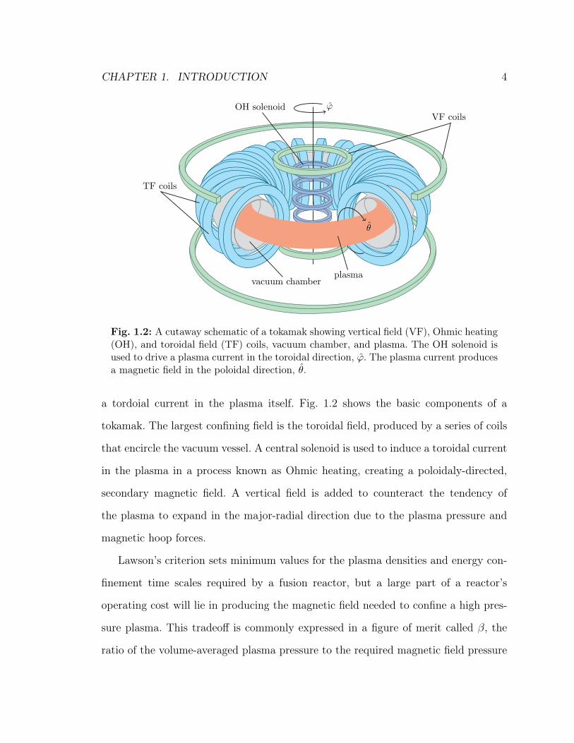
Fig. 1.2: A cutaway schematic of a tokamak showing vertical field (VF), Ohmic heating(OH), and toroidal field (TF) coils, vacuum chamber, and plasma. The OH solenoid isused to drive a plasma current in the toroidal direction, 𝜙. The plasma current producesa magnetic field in the poloidal direction, 𝜃.
a tordoial current in the plasma itself. Fig. 1.2 shows the basic components of a
tokamak. The largest confining field is the toroidal field, produced by a series of coils
that encircle the vacuum vessel. A central solenoid is used to induce a toroidal current
in the plasma in a process known as Ohmic heating, creating a poloidaly-directed,
secondary magnetic field. A vertical field is added to counteract the tendency of
the plasma to expand in the major-radial direction due to the plasma pressure and
magnetic hoop forces.
Lawson’s criterion sets minimum values for the plasma densities and energy con-
finement time scales required by a fusion reactor, but a large part of a reactor’s
operating cost will lie in producing the magnetic field needed to confine a high pres-
sure plasma. This tradeoff is commonly expressed in a figure of merit called 𝛽, the
ratio of the volume-averaged plasma pressure to the required magnetic field pressure
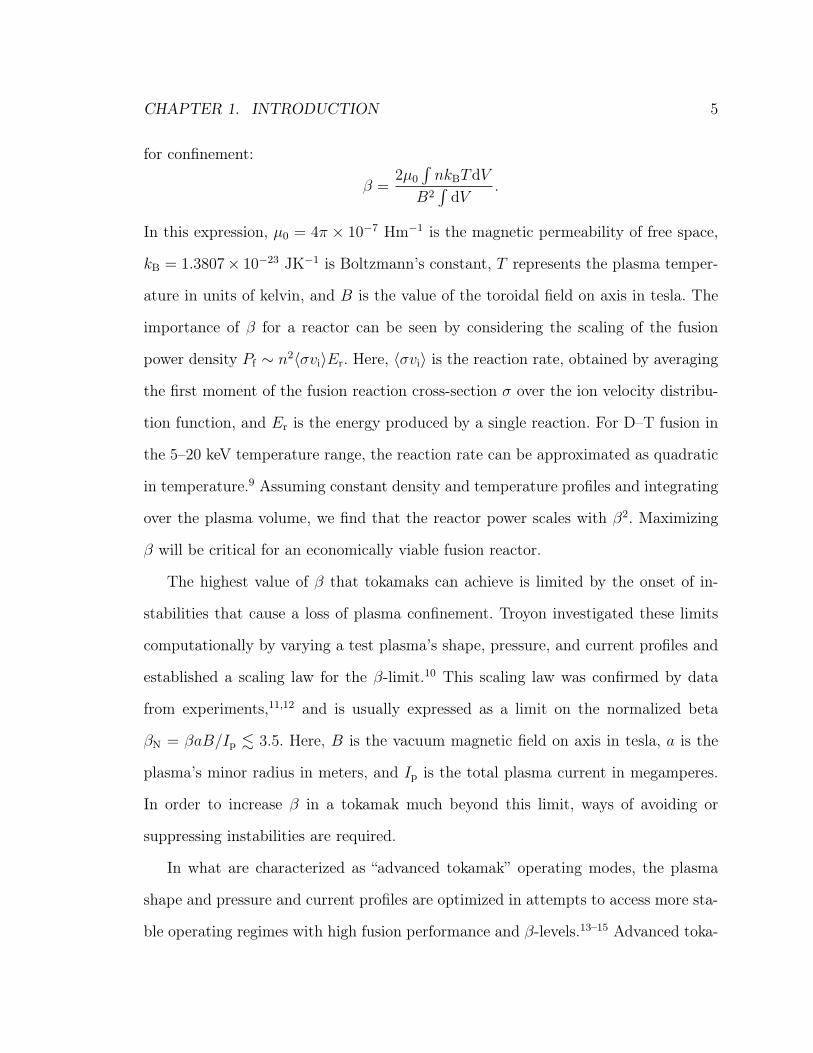
CHAPTER 1. INTRODUCTION 5
for confinement:
𝛽 =2𝜇0
∫𝑛𝑘B𝑇d𝑉
𝐵2∫
d𝑉.
In this expression, 𝜇0 = 4𝜋 × 10−7 Hm−1 is the magnetic permeability of free space,
𝑘B = 1.3807× 10⁻²³ JK−1 is Boltzmann’s constant, 𝑇 represents the plasma temper-
ature in units of kelvin, and 𝐵 is the value of the toroidal field on axis in tesla. The
importance of 𝛽 for a reactor can be seen by considering the scaling of the fusion
power density 𝑃f ∼ 𝑛2⟨𝜎𝑣i⟩𝐸r. Here, ⟨𝜎𝑣i⟩ is the reaction rate, obtained by averaging
the first moment of the fusion reaction cross-section 𝜎 over the ion velocity distribu-
tion function, and 𝐸r is the energy produced by a single reaction. For D–T fusion in
the 5–20 keV temperature range, the reaction rate can be approximated as quadratic
in temperature.9 Assuming constant density and temperature profiles and integrating
over the plasma volume, we find that the reactor power scales with 𝛽2. Maximizing
𝛽 will be critical for an economically viable fusion reactor.
The highest value of 𝛽 that tokamaks can achieve is limited by the onset of in-
stabilities that cause a loss of plasma confinement. Troyon investigated these limits
computationally by varying a test plasma’s shape, pressure, and current profiles and
established a scaling law for the 𝛽-limit.10 This scaling law was confirmed by data
from experiments,11,12 and is usually expressed as a limit on the normalized beta
𝛽N = 𝛽𝑎𝐵/𝐼p . 3.5. Here, 𝐵 is the vacuum magnetic field on axis in tesla, 𝑎 is the
plasma’s minor radius in meters, and 𝐼p is the total plasma current in megamperes.
In order to increase 𝛽 in a tokamak much beyond this limit, ways of avoiding or
suppressing instabilities are required.
In what are characterized as “advanced tokamak” operating modes, the plasma
shape and pressure and current profiles are optimized in attempts to access more sta-
ble operating regimes with high fusion performance and 𝛽-levels.13–15 Advanced toka-

CHAPTER 1. INTRODUCTION 6
mak scenarios are characterized by high values of 𝛽N, high fractions of self-driven, or
“bootstrap” current, and steep gradients in the temperature and density profiles near
the plasma edge. These operating regimes offer stability against so-called ballooning
modes with a high toroidal mode number 𝑛, but low-𝑛, external kink modes remain
unstable.16
The external kink mode is a surface wave instability characterized by a kink-
like distortion of the plasma boundary. Its growth rate is inversely proportional to
the Alfvén time 𝜏A = 𝑎√𝜇0𝜌/𝐵, where 𝑎 is the plasma’s minor radius and 𝜌 =
𝑚i𝑛i+𝑚e𝑛e is the plasma’s mass density. Under typical fusion power plant conditions,
this timescale is on the order of microseconds. However, a conducting wall near the
plasma boundary can host eddy currents that interact with the plasma mode. The
resulting plasma–wall mode is termed a resistive wall mode (RWM), and its growth
rate is proportional to the magnetic flux penetration rate of the wall 1/𝜏w. It is possible
to construct a wall such that 𝜏w ≫ 𝜏A, and several experiments have shown that a
nearby conducting wall can provide access to 𝛽 values above the “no-wall” limit.17,18
Numerical modeling, theory and experiments have also shown that the RWM may
be stabilized by a combination of a nearby conducting wall and plasma rotation,19–21
but the velocities required for rotational stabilization in a tokamak burning plasma
experiment such as ITER may not be easily and consistently attainable.22 The physics
of the external kink and resistive wall modes will be discussed in greater detail in
Chapter 2.
1.3 Feedback control of resistive wall modes
In the absence of sufficient plasma rotation, the RWM may be stabilized by active
feedback using magnetic coils to oppose the perturbed magnetic flux of the mode.23
CHAPTER 1. INTRODUCTION 7
Magnetic feedback stabilization of the RWM has been achieved on the HBT-EP ex-
periment, first with a “smart shell” scheme in which an array of radial sensor and
control coils was used to imitate a perfectly conducting wall,24 and later using an op-
timized “mode control” system that employed digital spatial and temporal filtering to
detect and suppress the 𝑛 = 1 mode near the ideal wall limit.25 Success in stabilizing
the RWM has also been realized in the DIII-D and NSTX experiments using similar
methods.26–34
The mode control feedback schemes typically used spatial filtering to detect low-
𝑛 components of the perturbed magnetic field, discarding 𝑛 = 0 and higher-order
harmonics unrelated to the RWM. However, this filtering is not adequate to address
the deleterious effects of measurement noise and sensor pick-up due to other plasma
activity, such as edge-localized modes (ELMs).
Several model-based mode identification algorithms, most employing a Kalman ob-
server,35 have been proposed for tokamak RWM feedback and tested numerically.36–40
The Kalman filter produces a dynamic estimate for the state of a system of inter-
est by comparing an internal, linear model for the system with measurements.35,41
Neither the internal model nor the measurements need to be perfect for an estimate
to be produced. For example, in the case of RWM feedback, simulations that fully
account for interaction with eddy-currents in nearby conducting structures require
the use of three-dimensional electromagnetic codes such as valen or mars-f.42,43
These detailed calculations cannot yet be performed on the time scales necessary for
closed loop feedback, but models with reduced physics are used in feedback algorithm
designs. In the Kalman filter formulation, the relative emphasis on the internal model
versus the measurements can be adjusted.
All of the model-based feedback algorithms cited above use system models that
account for the dynamics of the RWM in the presence of control inputs and pas-

CHAPTER 1. INTRODUCTION 8
Fig. 1.3: A photo of the HBT-EP experiment showing toroidal and vertical field mag-nets and the vacuum vessel.
sive conducting structures in varying levels of detail, and show promise in increasing
feedback robustness in the presence of white noise and/or that due to ELMs. The al-
gorithm of In, et. al.39 was tested on an RWM-unstable DIII-D discharge and was able
to reduce pickup due to ELMs in feedback signals. However, none of the algorithms
cited above have system models that account for the possibility of a rotating mode.
Mode rotation is an important factor to consider when designing RWM feedback al-
gorithms, because feedback that is out of phase with the mode can easily excite and
drive the mode, rather than suppress it.25 In cases where the rotation rate of the
mode is changing on time scales close to the controller latency, the optimal phasing
between applied feedback and the unstable mode may be lost.
CHAPTER 1. INTRODUCTION 9
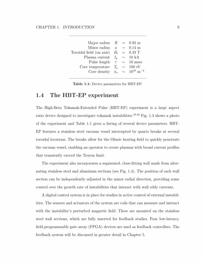
Major radius 𝑅 = 0.92 mMinor radius 𝑎 = 0.14 m
Toroidal field (on axis) 𝐵t = 0.33 TPlasma current 𝐼p ∼ 10 kA
Pulse length 𝜏 ∼ 10 msecCore temperature 𝑇e ∼ 100 eV
Core density 𝑛e ∼ 1019 m−3
Table 1.1: Device parameters for HBT-EP.
1.4 The HBT-EP experiment
The High-Beta Tokamak-Extended Pulse (HBT-EP) experiment is a large aspect
ratio device designed to investigate tokamak instabilities.18,44 Fig. 1.3 shows a photo
of the experiment and Table 1.1 gives a listing of several device parameters. HBT-
EP features a stainless steel vacuum vessel interrupted by quartz breaks at several
toroidal locations. The breaks allow for the Ohmic heating field to quickly penetrate
the vacuum vessel, enabling an operator to create plasmas with broad current profiles
that transiently exceed the Troyon limit.
The experiment also incorporates a segmented, close-fitting wall made from alter-
nating stainless steel and aluminum sections (see Fig. 1.4). The position of each wall
section can be independently adjusted in the minor radial direction, providing some
control over the growth rate of instabilities that interact with wall eddy currents.
A digital control system is in place for studies in active control of external instabil-
ities. The sensors and actuators of the system are coils that can measure and interact
with the instability’s perturbed magnetic field. These are mounted on the stainless
steel wall sections, which are fully inserted for feedback studies. Four low-latency,
field-programmable gate array (FPGA) devices are used as feedback controllers. The
feedback system will be discussed in greater detail in Chapter 5.

CHAPTER 1. INTRODUCTION 10
Fig. 1.4: The arrangement of the stainless steel and aluminum wall sections in theHBT-EP experiment.
1.5 Principal results
In HBT-EP and other tokamak experiments, attempts to control the resistive wall
mode with active magnetic feedback are sometimes hampered by system noise. Noise
can originate from many sources in tokamak experiments, including the plasma it-
self. This Thesis details the first successful application of a Kalman filter to the
problem of feedback control of rotating external kink instabilities in a tokamak. The
Kalman filter algorithm was developed and tested computationally using the reduced
Fitzpatrick–Aydemir model,45–47 and implemented on HBT-EP’s mode control sys-
tem for experiments with external kink-unstable plasmas. With the Kalman filter
algorithm, the feedback system was able to suppress and excite external kink modes,
even at noise levels that rendered feedback without the Kalman filter ineffective. The
system model used for the Kalman filter has only two parameters: the mode’s growth
rate and its rotation rate. These parameter settings were optimized in simulations
and experiments, and feedback performance was enhanced when a Kalman filter with
the optimal settings was used.

CHAPTER 1 REFERENCES 11
1.6 Outline of this Thesis
The remainder of this Thesis is organized as follows. Chapter 2 provides an overview
of the theory of the ideal external kink and resistive wall modes. In Chapter 3, com-
putational modeling of the external kink mode feedback problem is discussed, and
results for feedback simulations with and without the Kalman filter are presented.
Chapter 4 contains a discussion of the general Kalman filter equations and the design
of a Kalman filter for the external kink mode control problem in HBT-EP. In Chapter
5, the setup of feedback control hardware on HBT-EP is described, and an overview of
the feedback algorithm is given. General observations of external kink mode behavior
without feedback are discussed in Chapter 6, and Chapter 7 presents the results of
closed-loop Kalman filter feedback experiments.
The appendices cover some details of the implementation of the Kalman filter
algorithm on the FPGA controllers. Appendix A discusses general programming con-
siderations for the FPGAs, and Appendix B gives a formal description of the Kalman
filter algorithm.
Chapter 1 references1. R. A. Gross, Fusion Energy, John Wiley & Sons, New York, 1984.
2. J. D. Lawson, Proc. Phys. Soc. (London) B70, 6 (1957).
3. K. Miyamoto, Plasma Physics for Nuclear Fusion, The MIT Press, Cambridge,MA, 1989.
4. J. L. Bromberg, Fusion: Science, Politics, and the Invention of a New EnergySource, MIT Press, Cambridge, MA, 1982.
5. L. A. Artsimovich, Nuclear Fusion 12, 215 (1972).
6. J. D. Strachan, H. Adler, P. Alling, C. Ancher, H. Anderson, J. L. Anderson,D. Ashcroft, C. W. Barnes, G. Barnes, S. Batha, M. G. Bell, R. Bell, M. Bit-ter, W. Blanchard, N. L. Bretz, R. Budny, C. E. Bush, R. Camp, M. Caorlin,

CHAPTER 1 REFERENCES 12
S. Cauffman, Z. Chang, C. Z. Cheng, J. Collins, G. Coward, D. S. Darrow,J. DeLooper, and H. Duong, Phys. Rev. Lett. 72, 3526 (1994).
7. A. S. Kaye and the JET Team, Fusion Technology 34, 308 (1998).
8. I. P. B. Editors, I. P. E. G. Chairs, Co-Chairs, I. J. C. Team, and P. I. Unit,Nuclear Fusion 39, 2137 (1999).
9. J. Wesson, Tokamaks, Oxford University Press, New York, 3rd ed., 2004.
10. F. Troyon, R. Gruber, H. Saurenmann, S. Semenzato, and S. Succi, PlasmaPhysics and Controlled Fusion 26, 209 (1984).
11. F. Troyon and R. Gruber, Physics Letters A 110, 29 (1985).
12. F. Troyon, A. Roy, W. A. Cooper, F. Yasseen, and A. Turnbull, Plasma Physicsand Controlled Fusion 30, 1597 (1988).
13. C. Kessel, J. Manickam, G. Rewoldt, and W. M. Tang, Phys. Rev. Lett. 72,1212 (1994).
14. R. Goldston, S. Batha, R. Bulmer, D. Hill, A. Hyatt, S. Jardin, F. Levinton,S. Kaye, C. Kessel, E. Lazarus, J. Manickam, G. Neilson, W. Nevins, L. Perkins,G. Rewoldt, K. Thomassen, M. Zarnstorff, and the National TPX Physics Team,Plasma Physics and Controlled Fusion 36, B213 (1994).
15. T. S. Taylor, Plasma Physics and Controlled Fusion 39, B47 (1997).
16. E. J. Strait, Physics of Plasmas 1, 1415 (1994).
17. T. S. Taylor, E. J. Strait, L. L. Lao, M. Mauel, A. D. Turnbull, K. H. Burrell,M. S. Chu, J. R. Ferron, R. J. Groebner, R. J. L. Haye, B. W. Rice, R. T. Snider,S. J. Thompson, D. Wroblewski, and D. J. Lightly, Physics of Plasmas 2, 2390(1995).
18. T. H. Ivers, E. Eisner, A. Garofalo, R. Kombargi, M. E. Mauel, D. Maurer,D. Nadle, G. A. Navratil, M. K. V. Sankar, M. Su, E. Taylor, Q. Xiao, R. R.Bartsch, W. A. Reass, and G. A. Wurden, Physics of Plasmas 3, 1926 (1996).
19. A. Bondeson and D. J. Ward, Phys. Rev. Lett. 72, 2709 (1994).
20. R. Betti and J. P. Freidberg, Phys. Rev. Lett. 74, 2949 (1995).
21. A. M. Garofalo, E. J. Strait, L. C. Johnson, R. J. La Haye, E. A. Lazarus, G. A.Navratil, M. Okabayashi, J. T. Scoville, T. S. Taylor, and A. D. Turnbull, Phys.Rev. Lett. 89, 235001 (2002).

CHAPTER 1 REFERENCES 13
22. T. Hender, J. Wesley, J. Bialek, A. Bondeson, A. Boozer, R. Buttery, A. Garo-falo, T. Goodman, R. Granetz, Y. Gribov, O. Gruber, M. Gryaznevich, G. Giruzzi,S. Günter, N. Hayashi, P. Helander, C. Hegna, D. Howell, D. Humphreys, G. Huys-mans, A. Hyatt, A. Isayama, S. Jardin, Y. Kawano, A. Kellman, C. Kessel,H. Koslowski, R. L. Haye, E. Lazzaro, Y. Liu, V. Lukash, J. Manickam, S. Medvedev,V. Mertens, S. Mirnov, Y. Nakamura, G. Navratil, M. Okabayashi, T. Ozeki,R. Paccagnella, G. Pautasso, F. Porcelli, V. Pustovitov, V. Riccardo, M. Sato,O. Sauter, M. Schaffer, M. Shimada, P. Sonato, E. Strait, M. Sugihara, M. Takechi,A. Turnbull, E. Westerhof, D. Whyte, R. Yoshino, H. Zohm, and the ITPA MHDand Disruption and Magnetic Control Topical Group, Nuclear Fusion 47, S128(2007).
23. C. M. Bishop, Plasma Physics and Controlled Fusion 31, 1179 (1989).
24. C. Cates, M. Shilov, M. E. Mauel, G. A. Navratil, D. Maurer, S. Mukherjee,D. Nadle, J. Bialek, and A. Boozer, Physics of Plasmas 7, 3133 (2000).
25. A. J. Klein, D. A. Maurer, T. Sunn Pedersen, M. E. Mauel, G. A. Navratil,C. Cates, M. Shilov, Y. Liu, N. Stillits, and J. Bialek, Physics of Plasmas 12,040703 (2005).
26. A. Garofalo, E. Strait, J. Bialek, E. Fredrickson, M. Gryaznevich, T. Jensen,L. Johnson, R. L. Haye, G. Navratil, E. Lazarus, T. Luce, M. Makowski, M. Ok-abayashi, B. Rice, J. Scoville, A. Turnbull, M. Walker, and DIII-D Team, NuclearFusion 40, 1491 (2000).
27. M. Okabayashi, J. M. Bialek, M. S. Chance, M. S. Chu, E. D. Fredrickson, A. M.Garofalo, M. Gryaznevich, R. E. Hatcher, T. H. Jensen, L. C. Johnson, R. J. L.Haye, E. A. Lazarus, M. A. Makowski, J. Manickam, G. Navratil, J. T. Scoville,E. J. Strait, A. D. Turnbull, M. L. Walker, and DIII-D Team, Physics of Plasmas8, 2071 (2001).
28. A. M. Garofalo, M. S. Chu, E. D. Fredrickson, M. Gryaznevich, T. H. Jensen,L. C. Johnson, R. J. L. Haye, G. Navratil, M. Okabayashi, J. T. Scoville, E. J.Strait, A. D. Turnbull, and DIII-D Team, Nuclear Fusion 41, 1171 (2001).
29. M. Okabayashi, J. Bialek, M. S. Chance, M. S. Chu, E. D. Fredrickson, A. M.Garofalo, R. Hatcher, T. H. Jensen, L. C. Johnson, R. J. L. Haye, G. A. Navratil,H. Reimerdes, J. T. Scoville, E. J. Strait, A. D. Turnbull, M. L. Walker, andDIII-D Team, Plasma Physics and Controlled Fusion 44, B339 (2002).
30. E. J. Strait, J. M. Bialek, I. N. Bogatu, M. S. Chance, M. S. Chu, D. H. Edgell,A. M. Garofalo, G. L. Jackson, R. J. Jayakumar, T. H. Jensen, O. Katsuro-Hopkins, J. S. Kim, R. J. L. Haye, L. L. Lao, M. A. Makowski, G. A. Navratil,
CHAPTER 1 REFERENCES 14
M. Okabayashi, H. Reimerdes, J. T. Scoville, A. D. Turnbull, and DIII-D Team,Physics of Plasmas 11, 2505 (2004).
31. M. Okabayashi, J. Bialek, A. Bondeson, M. Chance, M. Chu, A. Garofalo,R. Hatcher, Y. In, G. Jackson, R. Jayakumar, T. Jensen, O. Katsuro-Hopkins,R. L. Haye, Y. Liu, G. Navratil, H. Reimerdes, J. Scoville, E. Strait, M. Takechi,A. Turnbull, P. Gohil, J. Kim, M. Makowski, J. Manickam, and J. Menard, Nu-clear Fusion 45, 1715 (2005).
32. A. Garofalo, G. Jackson, R. L. Haye, M. Okabayashi, H. Reimerdes, E. Strait,J. Ferron, R. Groebner, Y. In, M. Lanctot, G. Matsunaga, G. Navratil, W. Solomon,H. Takahashi, M. Takechi, A. Turnbull, and the DIII-D Team, Nuclear Fusion47, 1121 (2007).
33. S. A. Sabbagh, R. E. Bell, J. E. Menard, D. A. Gates, A. C. Sontag, J. M.Bialek, B. P. LeBlanc, F. M. Levinton, K. Tritz, and H. Yuh, Physical ReviewLetters 97, 045004 (2006).
34. J. Menard, M. Bell, R. Bell, S. Bernabei, J. Bialek, T. Biewer, W. Blanchard,J. Boedo, C. Bush, M. Carter, W. Choe, N. Crocker, D. Darrow, W. Davis,L. Delgado-Aparicio, S. Diem, C. Domier, D. D’Ippolito, J. Ferron, A. Field,J. Foley, E. Fredrickson, D. Gates, T. Gibney, R. Harvey, R. Hatcher, W. Hei-dbrink, K. Hill, J. Hosea, T. Jarboe, D. Johnson, R. Kaita, S. Kaye, C. Kessel,S. Kubota, H. Kugel, J. Lawson, B. LeBlanc, K. Lee, F. Levinton, J. N.C. Luh-mann, R. Maingi, R. Majeski, J. Manickam, D. Mansfield, R. Maqueda, R. Marsala,D. Mastrovito, T. Mau, E. Mazzucato, S. Medley, H. Meyer, D. Mikkelsen,D. Mueller, T. Munsat, J. Myra, B. Nelson, C. Neumeyer, N. Nishino, M. Ono,H. Park, W. Park, S. Paul, T. Peebles, M. Peng, C. Phillips, A. Pigarov, R. Pinsker,A. Ram, S. Ramakrishnan, R. Raman, D. Rasmussen, M. Redi, M. Rensink,G. Rewoldt, J. Robinson, P. Roney, A. Roquemore, E. Ruskov, P. Ryan, S. Sab-bagh, H. Schneider, C. Skinner, D. Smith, A. Sontag, V. Soukhanovskii, T. Steven-son, D. Stotler, B. Stratton, D. Stutman, D. Swain, E. Synakowski, Y. Takase,G. Taylor, K. Tritz, A. von Halle, M. Wade, R. White, J. Wilgen, M. Williams,J. Wilson, H. Yuh, L. Zakharov, W. Zhu, S. Zweben, R. Akers, P. Beiers-dorfer, R. Betti, T. Bigelow, M. Bitter, P. Bonoli, C. Bourdelle, C. Chang,J. Chrzanowski, L. Dudek, P. Efthimion, M. Finkenthal, E. Fredd, G. Fu, A. Glasser,R. Goldston, N. Greenough, L. Grisham, N. Gorelenkov, L. Guazzotto, R. Hawry-luk, J. Hogan, W. Houlberg, D. Humphreys, F. Jaeger, M. Kalish, S. Krashenin-nikov, L. Lao, J. Lawrence, J. Leuer, D. Liu, G. Oliaro, D. Pacella, R. Parsells,M. Schaffer, I. Semenov, K. Shaing, M. Shapiro, K. Shinohara, P. Sichta, X. Tang,R. Vero, M. Walker, and W. Wampler, Nuclear Fusion 47, S645 (2007).
35. R. E. Kalman, Transactions of the ASME–Journal of Basic Engineering 82, 35(1960).
CHAPTER 1 REFERENCES 15
36. C. M. Fransson, D. H. Edgell, D. A. Humphreys, and M. L. Walker, Physics ofPlasmas 10, 3961 (2003).
37. A. K. Sen, M. Nagashima, and R. W. Longman, Physics of Plasmas 10, 4350(2003).
38. Z. Sun, A. K. Sen, and R. W. Longman, Physics of Plasmas 13, 012512 (2006).
39. Y. In, J. S. Kim, D. H. Edgell, E. J. Strait, D. A. Humphreys, M. L. Walker,G. L. Jackson, M. S. Chu, R. Johnson, R. J. L. Haye, M. Okabayashi, A. M.Garofalo, and H. Reimerdes, Physics of Plasmas 13, 062512 (2006).
40. O. Katsuro-Hopkins, J. Bialek, D. Maurer, and G. Navratil, Nuclear Fusion 47,1157 (2007).
41. R. G. Brown and P. Y. C. Hwang, Introduction to Random Signals and AppliedKalman Filtering, John Wiley & Sons, New York, 3rd ed., 1997.
42. J. Bialek, A. H. Boozer, M. E. Mauel, and G. A. Navratil, Physics of Plasmas8, 2170 (2001).
43. Y. Q. Liu, A. Bondeson, C. M. Fransson, B. Lennartson, and C. Breitholtz,Physics of Plasmas 7, 3681 (2000).
44. M. K. V. Sankar, E. Eisner, A. Garofalo, D. Gates, T. H. Ivers, R. Kombargi,M. E. Mauel, D. Maurer, D. Nadle, G. A. Navratil, and Q. Xiao, Journal ofFusion Energy 12, 303 (1993).
45. M. Mauel, J. Bialek, A. Boozer, C. Cates, R. James, O. Katsuro-Hopkins,A. Klein, Y. Liu, D. Maurer, D. Maslovsky, G. Navratil, T. Pedersen, M. Shilov,and N. Stillits, Nuclear Fusion 45, 285 (2005).
46. R. Fitzpatrick, Physics of Plasmas 9, 3459 (2002).
47. R. Fitzpatrick and A. Y. Aydemir, Nuclear Fusion 36, 11 (1996).

Chapter 2
Physics of the tokamak external kink
mode
The ideal, external kink instability is a helical perturbation to the plasma’s surface
and magnetic field that grows on an Alfvénic time scale. The stability of tokamak
plasmas to external kink modes can be analyzed using the equations of ideal mag-
netohydrodynamics (MHD). In general, the stability of an MHD equilibrium can be
investigated by determining whether a displacement raises or lowers the potential en-
ergy of the equilibrium. In this Chapter, we will see that equilibria with large current
density gradients near the plasma’s edge can be unstable to external kink modes.
The presence of nearby conducting structures can significantly alter the growth rate
of the external kink through eddy current interactions, resulting in a resistive wall
mode (RWM). Although the RWM remains a 𝛽-limiting instability for tokamaks, it
can be stabilized by plasma rotation or feedback with magnetic coils.
16

CHAPTER 2. PHYSICS OF THE TOKAMAK EXTERNAL KINK MODE 17
2.1 Ideal magnetohydrodynamics
Ideal MHD is the simplest model that describes the macroscopic equilibria of mag-
netically confined plasmas and the stability of these equilibria. Full derivations of this
model and further discussions of its implications for tokamak plasmas are given in a
number of textbooks.1–3
The equations of ideal MHD are derived by taking velocity-space moments of the
Maxwell-Boltzmann equations and employing a number of simplifying assumptions.
They describe the evolution of the plasma’s mass density 𝜌 ≈ 𝑚i𝑛, scalar pressure
𝑝 = 𝑛(𝑇e + 𝑇i) = 𝑛𝑇 , mass-flow ≈ i, and current density = 𝑒𝑛(i − e), along
with the magnetic and electric fields, and .
The mass-continuity and momentum equations,
𝜕𝜌
𝜕𝑡+ ∇ · (𝜌) = 0 and (2.1)
𝜌(𝜕
𝜕𝑡+ · ∇) = × − ∇𝑝, (2.2)
express conservation of mass and force balance for the plasma.
A relationship between the plasma current and the electric field is given by Ohm’s
law, for example,
+ × = 𝜂.
However, in ideal MHD, the plasma resistivity 𝜂 is taken to be zero, so Ohm’s law
becomes
+ × = 0. (2.3)
An interesting consequence of making the right-hand side of Eq. 2.3 zero is that the
magnetic flux through a surface moving with the plasma must be conserved. (This
CHAPTER 2. PHYSICS OF THE TOKAMAK EXTERNAL KINK MODE 18
can be seen by considering the time rate of change of the flux through such a surface.)
Adding the resistive term or other terms to Ohm’s law frees the magnetic field from
having to move with the plasma.
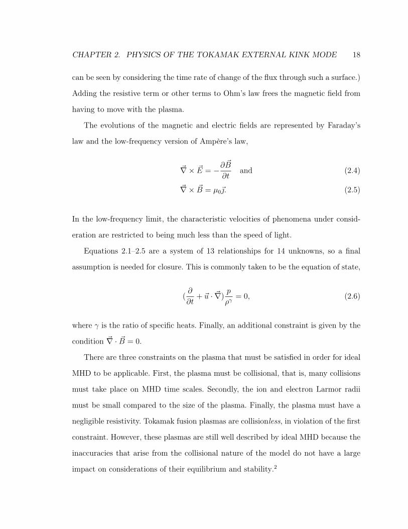
The evolutions of the magnetic and electric fields are represented by Faraday’s
law and the low-frequency version of Ampère’s law,
∇ × = −𝜕𝜕𝑡
and (2.4)
∇ × = 𝜇0. (2.5)
In the low-frequency limit, the characteristic velocities of phenomena under consid-
eration are restricted to being much less than the speed of light.
Equations 2.1–2.5 are a system of 13 relationships for 14 unknowns, so a final
assumption is needed for closure. This is commonly taken to be the equation of state,
(𝜕
𝜕𝑡+ · ∇)
𝑝
𝜌𝛾= 0, (2.6)
where 𝛾 is the ratio of specific heats. Finally, an additional constraint is given by the
condition ∇ · = 0.
There are three constraints on the plasma that must be satisfied in order for ideal
MHD to be applicable. First, the plasma must be collisional, that is, many collisions
must take place on MHD time scales. Secondly, the ion and electron Larmor radii
must be small compared to the size of the plasma. Finally, the plasma must have a
negligible resistivity. Tokamak fusion plasmas are collisionless, in violation of the first
constraint. However, these plasmas are still well described by ideal MHD because the
inaccuracies that arise from the collisional nature of the model do not have a large
impact on considerations of their equilibrium and stability.2

CHAPTER 2. PHYSICS OF THE TOKAMAK EXTERNAL KINK MODE 19
Fig. 2.1: Cross-sectional sketches of tokamak equilibrium quantities at low 𝛽: a) circularflux surfaces, b) poloidal and vacuum toroidal magnetic field profiles, and c) currentdensity and safety factor profiles.
2.2 Ideal MHD equilibrium
Ideal MHD equilibrium states are usually found by setting 𝜕/𝜕𝑡 and equal to zero
(although it is possible to have equilibria with = 0). From Eqs. 2.1–2.6, two non-
trivial relationships remain:
× = ∇𝑝, and (2.7)
∇ × = 𝜇0. (2.8)
By taking the dot product of Eq. 2.7 with and , we see that · ∇𝑝 = 0 and
· ∇𝑝 = 0. This implies that in MHD equilibrium, the magnetic field lines and lines
of current flow lie on contours of constant pressure. In toroidal configurations, these
contours form a series of nested toroidal surfaces called flux surfaces (see fig 2.1).
Other quantities of interest include the poloidal field that is generated by the plasma
current, current and pressure profiles, and the safety factor profile 𝑞(𝑟).
The safety factor gives the ratio of toroidal to poloidal transits a magnetic field line
makes as it maps out a flux surface in the plasma. For most of the magnetic surfaces
in a tokamak plasma, 𝑞 is either an high-order rational number, implying that many

CHAPTER 2. PHYSICS OF THE TOKAMAK EXTERNAL KINK MODE 20
Fig. 2.2: A magnetic field line with a 𝑚/𝑛 = 3/1 helicity makes three toroidal transitsfor every poloidal transit.
transits are made before the field line “bites its tail,” or an irrational number, implying
that the field line fills the entire surface. However, 𝑞(𝑟) is continuous across the plasma,
so a small number of surfaces are low-order rationals, such as 𝑞 = 𝑚/𝑛 = 3/1 (see
figure 2.2). These surfaces are associated with tokamak instabilities that are resonant
with the helicity of the local magnetic field line.
2.3 Stability of ideal MHD equilibria
The stability of MHD equilibria can be considered by linearizing the ideal MHD
equations about an equilibrium and analyzing the effect of a small displacement 𝜉. If
the change in potential energy associated with a given displacement is negative, then
the plasma equilibrium is unstable to that displacement.
To analyze the stability of an equilibrium specified by 0(), 0(), 𝑝0(), and
0() = 0, we linearize the ideal MHD equations (2.1–2.6) about the equilibrium
quantities, assuming that they satisfy Eqs. 2.7, 2.8, and ∇ · 0 = 0. A perturbation
expansion of the form 𝑌 (, 𝑡) = 𝑌0() + 𝑌1(, 𝑡) is used, where 𝑌 represents any of
the vector or scalar quantities in the ideal MHD equations. Terms that are second
order in the perturbation, such as 1 · ∇1, are ignored, and the perturbed velocity
CHAPTER 2. PHYSICS OF THE TOKAMAK EXTERNAL KINK MODE 21
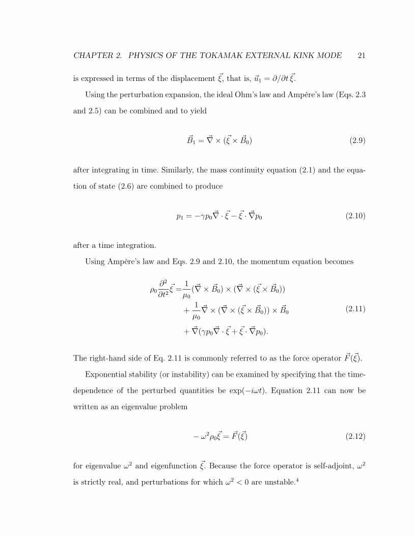
is expressed in terms of the displacement 𝜉, that is, 1 = 𝜕/𝜕𝑡 𝜉.
Using the perturbation expansion, the ideal Ohm’s law and Ampère’s law (Eqs. 2.3
and 2.5) can be combined and to yield
1 = ∇ × (𝜉 × 0) (2.9)
after integrating in time. Similarly, the mass continuity equation (2.1) and the equa-
tion of state (2.6) are combined to produce
𝑝1 = −𝛾𝑝0∇ · 𝜉 − 𝜉 · ∇𝑝0 (2.10)
after a time integration.
Using Ampère’s law and Eqs. 2.9 and 2.10, the momentum equation becomes
𝜌0𝜕2
𝜕𝑡2𝜉 =
1
𝜇0
(∇ × 0)× (∇ × (𝜉 × 0))
+1
𝜇0
∇ × (∇ × (𝜉 × 0))× 0
+ ∇(𝛾𝑝0∇ · 𝜉 + 𝜉 · ∇𝑝0).
(2.11)
The right-hand side of Eq. 2.11 is commonly referred to as the force operator 𝐹 (𝜉).
Exponential stability (or instability) can be examined by specifying that the time-
dependence of the perturbed quantities be exp(−𝑖𝜔𝑡). Equation 2.11 can now be
written as an eigenvalue problem
− 𝜔2𝜌0𝜉 = 𝐹 (𝜉) (2.12)
for eigenvalue 𝜔2 and eigenfunction 𝜉. Because the force operator is self-adjoint, 𝜔2
is strictly real, and perturbations for which 𝜔2 < 0 are unstable.4
CHAPTER 2. PHYSICS OF THE TOKAMAK EXTERNAL KINK MODE 22
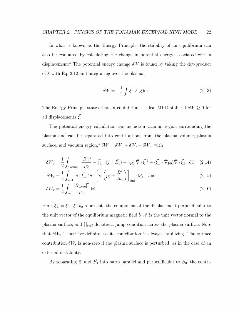
In what is known as the Energy Principle, the stability of an equilibrium can
also be evaluated by calculating the change in potential energy associated with a
displacement.5 The potential energy change 𝛿𝑊 is found by taking the dot-product
of 𝜉 with Eq. 2.12 and integrating over the plasma,
𝛿𝑊 = −1
2
∫𝜉 · 𝐹 (𝜉)d. (2.13)
The Energy Principle states that an equilibrium is ideal MHD-stable if 𝛿𝑊 ≥ 0 for
all displacements 𝜉.
The potential energy calculation can include a vacuum region surrounding the
plasma and can be separated into contributions from the plasma volume, plasma
surface, and vacuum region,4 𝛿𝑊 = 𝛿𝑊p + 𝛿𝑊s + 𝛿𝑊v, with
𝛿𝑊p =1
2
∫plasma
[|𝐵1|2
𝜇0
− 𝜉⊥ · (× 1) + 𝛾𝑝0|∇ · 𝜉|2 + (𝜉⊥ · ∇𝑝0)∇ · 𝜉⊥]
d, (2.14)
𝛿𝑊s =1
2
∫surf
| · 𝜉⊥|2 ·[∇
(𝑝0 +
𝐵20
2𝜇0
)]surf
d𝑆, and (2.15)
𝛿𝑊v =1
2
∫vac
|𝐵1,vac|2
𝜇0
d. (2.16)
Here, 𝜉⊥ = 𝜉 − 𝜉 · 0 represents the component of the displacement perpendicular to
the unit vector of the equilibrium magnetic field 0, is the unit vector normal to the
plasma surface, and [ ]surf denotes a jump condition across the plasma surface. Note
that 𝛿𝑊v is positive-definite, so its contribution is always stabilizing. The surface
contribution 𝛿𝑊s is non-zero if the plasma surface is perturbed, as in the case of an
external instability.
By separating 0 and 1 into parts parallel and perpendicular to 0, the contri-

CHAPTER 2. PHYSICS OF THE TOKAMAK EXTERNAL KINK MODE 23
bution from the plasma can be manipulated into what is called the intuitive form,6,7
𝛿𝑊p =1
2
∫plasma
[|𝐵1,⊥|2
𝜇0
+𝐵2
0
𝜇0
|∇ · 𝜉⊥ + 2𝜉⊥ · |2 + 𝛾𝑝0|∇ · 𝜉|2
− 2(𝜉⊥ · ∇𝑝0)( · 𝜉⊥)− 𝑗0,‖(𝜉⊥ × 0) · 1
]d. (2.17)
Here, 𝜅 = 0 · ∇0 is the curvature vector of the equilibrium magnetic field. The
first three terms in Eq. 2.17 are stabilizing and give the energy required to bend and
compress magnetic field lines, and the energy required to compress the plasma. The
fourth term is destabilizing when the field line curvature points in the direction
of increasing pressure. This circumstance always arises somewhere in toroidal con-
figurations, such as the tokamak, and instabilities that are caused by this effect are
called pressure-driven or “ballooning” instabilities. Parallel equilibrium currents are
the destabilizing factor in the last term, and the source of current-driven instabilities.
When gradients in the parallel current density occur near rational surfaces, internal
or external kink instabilities are the result, depending on the location of the rational
surface in question. With non-zero plasma resistivity, gradients in the parallel current
that lie inside the plasma can also open magnetic islands in what are known as tearing
modes.
2.4 The ideal, external kink mode
The ideal, external kink mode is a helical perturbation to the plasma’s surface and
magnetic field (see Fig. 2.3) that can be destabilized by a small irregularity in the
plasma’s shape or a magnetic error field if the current density gradient is sufficiently
strong near the edge of the plasma. In the absence of nearby conducting structures, ex-
ternal kink modes have growth rates proportional to the Alfvén time 𝜏A = 𝑎√𝜇0𝜌/𝐵,
CHAPTER 2. PHYSICS OF THE TOKAMAK EXTERNAL KINK MODE 24
Fig. 2.3: An (𝑚,𝑛) = (3, 1) perturbation to a toroidal surface, such as might beobserved during the onset of an external kink mode.
on the order of microseconds in most tokamak experiments.
Shafranov completed an analytical analysis of the external kink in a cylindrical
geometry with a flat current current density profile, calculating the growth rate as
a function of the mode helicity and safety-factor.8 Fig. 2.4 shows the results of this
calculation for 𝑚 = 1, 2, and 3 modes. More realistic Gaussian and parabolic current
density profiles were evaluated numerically, showing that stability was improved as
either a) the current density profile became more peaked in the center, or b) an ideally
conducting wall was brought closer to the edge of the plasma.
A more detailed analysis can be done for large aspect ratio tokamaks by expanding
𝛿𝑊 using the inverse aspect ratio 𝜖 ≡ 𝑎/𝑅0 as a parameter of smallness. Perturbations
may then be written in the form 𝜉 = 𝜉𝑟(𝑟) exp[𝑖(𝑚𝜃 − 𝑛𝜙)]. Using this expansion,
Wesson numerically investigated the stability of parametric current density profiles
of the form 𝑗𝜙(𝑟) = 𝑗𝜙0[1 − (𝑟/𝑎)2]𝜈 .9 In Wesson’s model, the center of the current
density profile becomes more sharply peaked with increasing 𝜈, and setting 𝜈 = 0 gives
a completely flat profile. A region of external kink stability was found for 𝑞𝑎 > 1 and
𝜈 & 1, but a portion of this space is unstable to ideal internal modes and (resistive)
tearing modes.
CHAPTER 2. PHYSICS OF THE TOKAMAK EXTERNAL KINK MODE 25
Fig. 2.4: Normalized growth rates of toroidal mode number 𝑛 = 1 and poloidal modenumbers 𝑚 = 1, 2, and 3 ideal, external kink modes as a function of the edge-safetyfactor from Shafranov’s analysis.
At high 𝛽, pressure profile effects can impact external kink mode stability as well.
The stability of several classes of parametric pressure and current density profiles in
the DIII-D tokamak was investigated numerically by Howl, et. al ,10 with the finding
that the 𝛽-limit for the 𝑛 = 1 kink mode was strongly affected by the shaping of both
profiles.
2.5 The resistive wall mode
Modern tokamak experiments usually have metal vacuum vessel walls and other con-
ducting structures near the surface of the plasma, and these objects can sustain eddy
currents that interact with the external kink mode and slow the mode’s growth rate.
The perturbed magnetic flux of the kink mode induces wall eddy currents that in
turn create an opposing flux, temporarily preventing the kink mode’s flux from pene-
trating the wall. However, it is not practical to have a perfectly conducting wall near
the edge of a tokamak plasma, so eddy currents in the wall must decay on the time
scale 𝜏w = 𝐿w/𝑅w. This interaction of wall eddy currents with the external kink is

CHAPTER 2. PHYSICS OF THE TOKAMAK EXTERNAL KINK MODE 26
called the resistive wall mode (RWM), and its growth time is determined by 𝜏w ≫ 𝜏A.
Without a mechanism for energy dissipation in the plasma, it is not possible to sta-
bilize an equilibrium that is ideally unstable without a conducting wall by adding a
wall of finite conductivity.11
Our discussion so far has ignored the physics of equilibrium plasma rotation and
energy dissipation, but these effects play an important role in RWM stability. For the
case of a rotating plasma with zero dissipation, there are two distinct possibilities: a
rotating, quickly growing external kink mode, and a non-rotating mode that grows
on the time scale of the wall.12 Modes of the second type are commonly referred to
as being “locked” to the wall.
Bondeson and Ward numerically analyzed the combined effects of plasma rotation
and dissipation with the finding that both the ideal kink and RWM could be stable up
to about 30% of the no-wall 𝛽-limit with rotation velocities around a few percent of
the Alfvén velocity and proper radial placement of the wall.13 Rotational stabilization
of ideally unstable DIII-D discharges made at comparable rotation velocities was also
observed.14 Further theoretical analysis that included various dissipation mechanisms
yielded cubic dispersion relations in which all three roots could be stabilized with
sufficient rotation and dissipation.15,16
Some dissipative mechanism is required for rotational stabilization of the RWM
because dissipation leads to a torque between a rotating plasma and the perturbed
magnetic field of the instability. A rotating mode also experiences a torque from wall
eddy currents. When the balance between these torques is such that the instability
rotates on a time scale that is much faster than 𝜏w, its flux is not able to penetrate
the wall.17
In addition to rotational stabilization, the RWM can be stabilized by feedback with
magnetic coils that oppose perturbed flux of the mode. Feedback is made possible by

CHAPTER 2 REFERENCES 27
the fact that the RWM’s growth rate is proportional to 1/𝜏w, typically several orders
of magnitude slower than the ideal kink’s Alfvénic growth rate. However, the presence
of the wall can limit the effectiveness of feedback because control coils, which apply
radial magnetic fields, must also push their flux through the wall. Feedback systems
can also encounter difficulties with spurious pickup from other ambient magnetic
activity, leading to excitation of the system when an RWM instability is not present.18
Additionally, the RWM can change shape when feedback is applied, in what is known
as a “non-rigid” response.19–21 The application of techniques from modern control
theory to exploit physics knowledge of the RWM in picking optimal feedback gains and
discriminating the unstable mode from noise is currently an active area of research.
One technique, the Kalman filter, will be discussed in detail in Chapter 4.
Chapter 2 references1. G. Bateman, MHD Instablilities, The MIT Press, Cambridge, MA, 1978.
2. J. P. Freidberg, Ideal Magnetohydrodynamics, Plenum Press, New York, 1987.
3. J. Wesson, Tokamaks, Oxford University Press, New York, 3rd ed., 2004.
4. I. B. Bernstein, E. A. Frieman, M. D. Kruskal, and R. M. Kulsrud, Proceedingsof the Royal Society of London. Series A, Mathematical and Physical Sciences244, 17 (1958).
5. S. Lundquist, Phys. Rev. 83, 307 (1951).
6. H. P. Furth, J. Killeen, M. N. Rosenbluth, and B. Coppi, Stabilization by shearand negative 𝑉 ′′, in Plasma Physics and Controlled Nuclear Fusion Research1964, volume 1, page 103, Vienna, 1965, IAEA.
7. J. M. Greene and J. L. Johnson, Plasma Physics 10, 729 (1968).
8. V. D. Shafranov, Soviet Physics – Technical Physics 15, 175 (1970).
9. J. A. Wesson, Nuclear Fusion 18, 87 (1978).
10. W. Howl, A. D. Turnbull, T. S. Taylor, L. L. Lao, F. J. Helton, J. R. Ferron,and E. J. Strait, Physics of Fluids B: Plasma Physics 4, 1724 (1992).

CHAPTER 2 REFERENCES 28
11. D. Pfirsch and H. Tasso, Nuclear Fusion 11, 259 (1971).
12. L. E. Zakharov and S. V. Putvinskii, Soviet Journal of Plasma Physics 13, 118(1987).
13. A. Bondeson and D. J. Ward, Phys. Rev. Lett. 72, 2709 (1994).
14. E. J. Strait, T. S. Taylor, A. D. Turnbull, J. R. Ferron, L. L. Lao, B. Rice,O. Sauter, and S. J. Thompson, Physical Review Letters 74, 2483 (1995).
15. R. Betti and J. P. Freidberg, Phys. Rev. Lett. 74, 2949 (1995).
16. M. Chu, J. Greene, T. Jensen, R. Miller, A. Bondeson, R. Johnson, and M. Mauel,Physics of Plasmas 2, 2236 (1995).
17. A. H. Boozer, Physics of Plasmas 10, 1458 (2003).
18. C. M. Fransson, D. H. Edgell, D. A. Humphreys, and M. L. Walker, Physics ofPlasmas 10, 3961 (2003).
19. M. Okabayashi, J. M. Bialek, M. S. Chance, M. S. Chu, E. D. Fredrickson, A. M.Garofalo, M. Gryaznevich, R. E. Hatcher, T. H. Jensen, L. C. Johnson, R. J. L.Haye, E. A. Lazarus, M. A. Makowski, J. Manickam, G. Navratil, J. T. Scoville,E. J. Strait, A. D. Turnbull, M. L. Walker, and DIII-D Team, Physics of Plasmas8, 2071 (2001).
20. S. A. Sabbagh, R. E. Bell, J. E. Menard, D. A. Gates, A. C. Sontag, J. M.Bialek, B. P. LeBlanc, F. M. Levinton, K. Tritz, and H. Yuh, Physical ReviewLetters 97, 045004 (2006).
21. T. Sunn Pedersen, D. A. Maurer, J. Bialek, O. Katsuro-Hopkins, J. M. Hanson,M. E. Mauel, R. James, A. Klein, Y. Liu, and G. A. Navratil, Nuclear Fusion47, 1293 (2007).
Chapter 3
Simulating external kink mode
feedback
Simulations play a crucial role in the design and understanding of resistive wall mode
(RWM) experiments. In this Chapter, a model for RWM activity in the HBT-EP
experiment based on the reduced Fitzpatrick–Aydemir equations is introduced. The
model accounts for the interaction of the instability with a resistive wall, plasma
rotation and dissipation, and magnetic feedback. Stabilization of the mode is possible
with proportional gain feedback, but the addition of noise to measurements used to
compute the feedback voltage results in increased control power consumption and
poorer suppression of the instability.
3.1 Models for the resistive wall mode
Simulating the interaction of an external kink instability with a nearby conducting
wall is a somewhat difficult problem if the wall and plasma have complicated, three
dimensional shapes as they do in many experiments. In the case of tokamaks, the
29

CHAPTER 3. SIMULATING EXTERNAL KINK MODE FEEDBACK 30
unperturbed plasma can safely be assumed to be symmetric about its vertical axis,
but many walls have more complicated symmetries, or no symmetry at all.
Experiments also have arrays of magnetic sensor and control coils for feedback
stabilization experiments, and it is desirable to simulate the effect of feedback to aid
in understanding the results of present experiments and the design of future ones.
The inclusion of feedback in simulations adds another level of complexity because
four types of non-trivial interactions between currents in different elements of the
system must now be considered: plasma–wall, plasma–coil, wall–coil, and coil–coil.
Boozer has devised a general method1–4 for accounting for the mutual interactions
of currents in various conductors in RWM experiments that is implemented in the
valen finite-element code.5 In Boozer’s prescription, the interaction between a set
of currents on the plasma surface and currents in the wall and coils are character-
ized by circuit equations. (In actual tokamak plasmas, currents inside the plasma
can contribute to the mode as well, but this contribution can be represented with
an equivalent set of currents at the surface of the plasma.) Each plasma mode is
characterized by a dimensionless stability parameter 𝑠𝑖, and a dimensionless torque
parameter 𝛼𝑖. In the case of a single plasma mode, the stability parameter can be
written as the normalized energy of the mode, 𝑠 = −𝛿𝑊/𝛿𝑊v, where 𝛿𝑊 and 𝛿𝑊v are
defined in Eqs. 2.13 and 2.16.3 In the case of 𝛼 = 0, the RWM is unstable for 𝑠 > 0,
and when 𝑠 is greater than some critical value 𝑠crit, the quickly growing external kink
mode is unstable. Increasing 𝛼 has a stabilizing effect.
The magnetic flux of the modes at the plasma surface Φ is expressed in terms of
the current in all of the plasma modes 𝐼, the currents in the wall 𝐼w, and the currents
in the feedback coils 𝐼f ,
Φ = 𝐿𝐼 +𝑀pw𝐼w +𝑀pf𝐼f ,
CHAPTER 3. SIMULATING EXTERNAL KINK MODE FEEDBACK 31
where 𝐿 is an inductance matrix for the modes on the plasma surface, 𝑀pw is a matrix
containing the mutual inductances between the plasma modes and circuit elements
in the wall, and 𝑀pf contains the mutual inductances between the feedback coils and
plasma modes. Similarly, the flux at the wall can be expressed as
Φw = 𝑀wp𝐼 + 𝐿w𝐼w +𝑀wf𝐼f .
In the scalar, “single-circuit,” limit of these equations, a dimensionless coefficient
for expressing the coupling between the plasma and the wall can be defined as 𝑐 =
𝑀pw𝑀wp(𝐿𝐿w)−1. Another dimensionless number 𝑐f = 1−𝑀pw𝑀wf(𝐿w𝑀pf)−1 is used
to characterize the coupling between the plasma and feedback control coils.
An analytical theory for the RWM from Fitzpatrick and Aydemir6,7 differs from
the Boozer approach in that it employs a cylindrical plasma and resistive wall. The
advantage of this formulation is that the essential physics of the interaction of a
rotating external kink mode with a wall and plasma dissipation is captured in an
analytic, cubic dispersion relation. Good agreement between the Fitzpatrick–Aydemir
model and external kink mode behavior on HBT-EP was found for modes near the
marginal stability limit.8
3.2 The reduced Fitzpatrick–Aydemir equations
The reduced Fitzpatrick–Aydemir model is obtained by taking a high-dissipation
limit, resulting in a system of ordinary differential equations for the flux of the mode
at the plasma surface 𝜓𝑎 and the flux at the wall 𝜓w in the presence of a control coil
flux 𝜓c.9
CHAPTER 3. SIMULATING EXTERNAL KINK MODE FEEDBACK 32
d
d𝑡= 𝐴+ 𝜓c, (3.1)
where
=
⎛⎜⎝𝜓𝑎
𝜓w
⎞⎟⎠ , 𝐴 =
⎛⎜⎝(1− 𝑠− 𝑖)𝛾2MHD
𝜈d−𝛾2
MHD
𝜈d√
𝑐
𝛾w√
𝑐1−𝑐
− 𝛾w
1−𝑐
⎞⎟⎠ ,
and =
⎛⎜⎝ −𝑐f𝛾2MHD
𝜈d
𝛾w(1−𝑐𝑐f)1−𝑐
⎞⎟⎠ .
Equation 3.1 is easily and quickly integrated numerically, providing a convenient
testbed for control algorithms. The parameter 𝑠 ≡ 𝑠/𝑠crit characterizes the energy
of the mode as in the Boozer formulation, and the torque parameter is given by
≡ −Ω𝜈d/𝛾2MHD. Here, Ω is the angular rotation frequency of the plasma and 𝜈d
is the rate of plasma energy dissipation due to interaction with the magnetic field
of the mode. Frequencies in the model are normalized to the growth rate of ideal
MHD instabilities, 𝛾MHD, and 𝛾w = 1/𝜏w is the eddy current decay rate of the wall.
The scalar plasma–wall and plasma–feedback coupling coefficients, 𝑐 and 𝑐f , were
obtained by fitting the results of a valen model for HBT-EP to a dispersion relation
from Ref. 10 that accounted for a wall like that of HBT-EP, that is, a wall with two
characteristic time constants.11
The impact of 𝑠 and can be understood by considering the stability properties
of Eq. 3.1 with 𝜓c = 0. If the real part of one the eigenvalues of 𝐴 is greater than
zero, then an unstable, rotating mode exists with a complex growth rate equal to that
eigenvalue, 𝛾𝑘. Fig. 3.1 shows the transition between Re𝛾𝑘 < 0 and Re𝛾𝑘 > 0 as a
function of 𝑠 and . For a given value of the torque , the growth rate increases with
increasing mode energy 𝑠, eventually becoming greater than zero. As the torque is
CHAPTER 3. SIMULATING EXTERNAL KINK MODE FEEDBACK 33
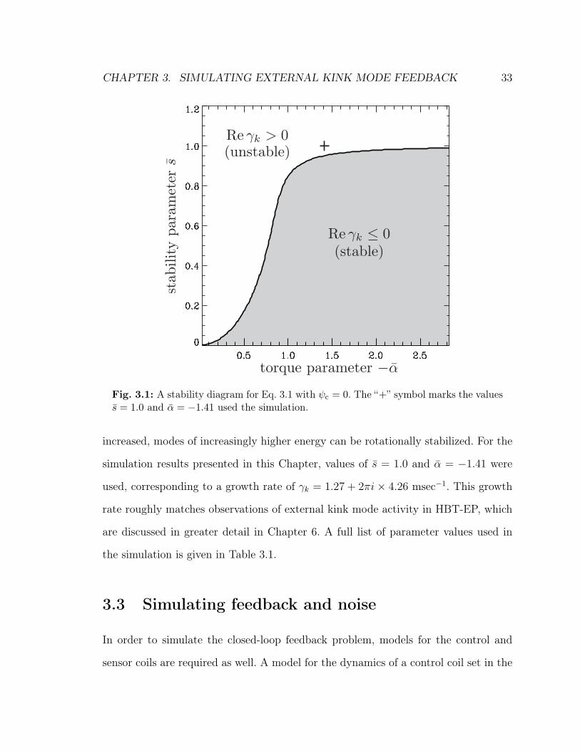
Fig. 3.1: A stability diagram for Eq. 3.1 with 𝜓c = 0. The “+” symbol marks the values𝑠 = 1.0 and = −1.41 used the simulation.
increased, modes of increasingly higher energy can be rotationally stabilized. For the
simulation results presented in this Chapter, values of 𝑠 = 1.0 and = −1.41 were
used, corresponding to a growth rate of 𝛾𝑘 = 1.27 + 2𝜋𝑖× 4.26 msec−1. This growth
rate roughly matches observations of external kink mode activity in HBT-EP, which
are discussed in greater detail in Chapter 6. A full list of parameter values used in
the simulation is given in Table 3.1.
3.3 Simulating feedback and noise
In order to simulate the closed-loop feedback problem, models for the control and
sensor coils are required as well. A model for the dynamics of a control coil set in the
CHAPTER 3. SIMULATING EXTERNAL KINK MODE FEEDBACK 34
reduced Fitzpatrick–Aydemir framework is given by12
d𝜓c
d𝑡+𝑅c
𝐿c
𝜓c =𝑀c
𝐿c
𝑉c, (3.2)
where 𝑅c and 𝐿c represent the resistance and inductance of the control coils, 𝑀c is
the coil–coil mutual inductance, and the control voltage 𝑉c is determined from 𝜓𝑎
and 𝜓w according to a feedback rule. When these quantities are specified, the coils’
magnetic flux 𝜓c can be obtained. Eq. 3.2 is approximate in that the direct coupling
between the control coils and the wall is neglected. However, this coupling is small
for HBT-EP in the frequency range of interest because the wall sections on which the
coils are mounted have negligible eddy current decay times (see Chapter 5). Eqs. 3.1
and 3.2 are integrated to obtain 𝜓𝑎, 𝜓w, and 𝜓c at each time step in the model.
Digital feedback algorithms currently in place on HBT-EP use a Discrete Fourier
Transform (DFT) to decompose toroidal sets of 5 poloidal-field sensor coil signals into
sin𝜙 and cos𝜙 𝑛 = 1 modes. In the model, the poloidal magnetic field is computed
from the plasma and wall fluxes12
𝐵p =3
𝑟w(1− 𝑐)[2√𝑐,−(𝑐+ 1)] · , (3.3)
and similarly decomposed into sine and cosine modes.
𝐵 cosp = Re[𝐵p + 𝑣]
𝐵 sinp = Re[e−𝑖𝜋/2(𝐵p + 𝑣)]
(3.4)
Here, 𝑟w is the minor radius of the wall, and 𝑣 represents white-spectrum, Gaussian
measurement noise. In the simulation, it is added as a complex-valued random number
at each time step. Eq. 3.3 neglects a contribution from the control flux 𝜓c. However,
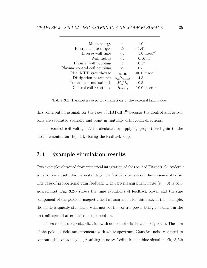
CHAPTER 3. SIMULATING EXTERNAL KINK MODE FEEDBACK 35
Mode energy 𝑠 1.0Plasma–mode torque −1.41
Inverse wall time 𝛾w 5.0 msec−1
Wall radius 𝑟w 0.16 mPlasma–wall coupling 𝑐 0.17
Plasma–control coil coupling 𝑐f 0.5Ideal MHD growth-rate 𝛾MHD 100.0 msec−1
Dissipation parameter 𝜈d/𝛾MHD 4.5Control coil mutual ind. 𝑀c/𝐿c 0.3
Control coil resistance 𝑅c/𝐿c 10.0 msec−1
Table 3.1: Parameters used for simulations of the external kink mode.
this contribution is small for the case of HBT-EP,13 because the control and sensor
coils are separated spatially and point in mutually orthogonal directions.
The control coil voltage 𝑉c is calculated by applying proportional gain to the
measurements from Eq. 3.4, closing the feedback loop.
3.4 Example simulation results
Two examples obtained from numerical integration of the reduced Fitzpatrick–Aydemir
equations are useful for understanding how feedback behaves in the presence of noise.
The case of proportional gain feedback with zero measurement noise (𝑣 = 0) is con-
sidered first. Fig. 3.2-a shows the time evolutions of feedback power and the sine
component of the poloidal magnetic field measurement for this case. In this example,
the mode is quickly stabilized, with most of the control power being consumed in the
first millisecond after feedback is turned on.
The case of feedback stabilization with added noise is shown in Fig. 3.2-b. The sum
of the poloidal field measurements with white spectrum, Gaussian noise 𝑣 is used to
compute the control signal, resulting in noisy feedback. The blue signal in Fig. 3.2-b

CHAPTER 3. SIMULATING EXTERNAL KINK MODE FEEDBACK 36
Fig. 3.2: Control power and sine poloidal field measurements from feedback simulationswith the reduced Fitzpatrick–Aydemir equations for cases with a) no added noise, andb) Gaussian noise added to poloidal field measurements. In the poloidal field measure-ments for part b), the black trace shows the measurements without added noise. Themeasurements with added noise (blue) are used to compute the feedback signal.
shows the sine component of poloidal field measurements plus noise. For comparison,
the poloidal field measurements without noise are overlaid in black. Here, feedback
retains its ability to suppress the unstable mode, but at the expense of increased
control power consumption compared with the noise-free case.
Because the simulation equations are linear, proportional gain feedback can sup-
press the instability with arbitrary amounts of added noise. However, nonlinear effects
such as controller saturation and latency can impair the ability to do successful feed-
back under noisy conditions. The impact of controller latency on feedback is less
obvious than that of saturation. Latency introduces a temporal phase-shift between
the output and input of the controller that is linear in frequency. If there is white-
spectrum noise in measurements, the phase-shift due to latency implies that some

CHAPTER 3 REFERENCES 37
frequency components of the noise will be phased for positive feedback.
In the next Chapter, an advanced tool for estimating the state of a noisy sys-
tem, the Kalman filter, will be introduced. The Kalman filter compares an internal
model for a system with measurements to produce an estimate that is optimal if the
uncertainties in the model and measurements have Gaussian probability distributions.
Chapter 3 references1. A. H. Boozer, Physics of Plasmas 5, 3350 (1998).
2. A. H. Boozer, Physics of Plasmas 6, 3180 (1999).
3. A. H. Boozer, Phys. Rev. Lett. 86, 5059 (2001).
4. A. H. Boozer, Physics of Plasmas 10, 1458 (2003).
5. J. Bialek, A. H. Boozer, M. E. Mauel, and G. A. Navratil, Physics of Plasmas8, 2170 (2001).
6. R. Fitzpatrick and A. Y. Aydemir, Nuclear Fusion 36, 11 (1996).
7. R. Fitzpatrick, Physics of Plasmas 9, 3459 (2002).
8. M. Shilov, C. Cates, R. James, A. Klein, O. Katsuro-Hopkins, Y. Liu, M. E.Mauel, D. A. Maurer, G. A. Navratil, T. S. Pedersen, N. Stillits, R. Fitzpatrick,and S. F. Paul, Physics of Plasmas 11, 2573 (2004).
9. M. Mauel, J. Bialek, A. Boozer, C. Cates, R. James, O. Katsuro-Hopkins,A. Klein, Y. Liu, D. Maurer, D. Maslovsky, G. Navratil, T. Pedersen, M. Shilov,and N. Stillits, Nuclear Fusion 45, 285 (2005).
10. R. Fitzpatrick, Physics of Plasmas 1, 2931 (1994).
11. M. E. Mauel, Model Parameter Fit to VALEN Calculations for HBT-EP,unpublished, 2004.
12. M. E. Mauel, J. Farrington, J. Bialek, O. Katsuro-Hopkins, A. Klein, D. A.Maurer, G. A. Navratil, and T. S. Pedersen, Kalman filters to reduce noiseeffects during external kink control, in Bull. Amer. Phys. Soc. Paper, pageBP1.00007, 2005.
13. A. J. Klein, High-speed digital mode control feedback on Magneto-hydrodynamicinstabilities in the HBT-EP tokamak, PhD thesis, Columbia University, 2005.

Chapter 4
The Kalman filter
The ability to control a physical system depends critically on knowledge of the sys-
tem’s state. For example, the controller in an oven must be able to determine the
oven’s temperature and engage a heating mechanism if the temperature is lower than
a prescribed reference. Uncertainties in measurements of the temperature would re-
sult in poor control. However, it is not difficult to imagine feedback control scenarios
in which measurements are less than perfect. In the case of RWM control, there may
be electrical pickup in sensor coils and cabling from external sources, including wall
currents and plasma activity not related to the mode. It is possible for the coils to
be misaligned or poorly calibrated. Additionally, sensor coils can be damaged during
plasma disruptions if they are not sufficiently shielded.
In light of these measurement difficulties, it is desirable to implement feedback
control algorithms that can compare measurements with internal knowledge of the
system dynamics. The Kalman filter provides a formalism for doing exactly this. Given
a linear model and measurements, the Kalman filter produces a dynamic estimate for
the state of a system that is optimal if uncertainties in the model and measurements
are Gaussian. In this Chapter, the Kalman filter is introduced and filter matrices for38
CHAPTER 4. THE KALMAN FILTER 39
observing the external kink mode in HBT-EP are given. In simulations with added
noise, we will see that using the Kalman filter can dramatically reduce the amount of
control power required to suppress the instability.
4.1 The linear control problem
The results from modern control theory discussed in this Chapter apply to physical
systems whose time evolution can be characterized by first-order, linear ordinary
differential equations (ODEs) of the form
d
d𝑡(𝑡) = 𝐴(𝑡).
The matrix 𝐴 characterizes the dynamics of the system state (𝑡). The state vec-
tor contains information needed to observe and control the system. For example, in
simple mechanical systems, the state might be a vector containing the position and
momentum of an object, = [𝑞, 𝑝]. In the previous Chapter, the system state in the
reduced Fitzpatrick–Aydemir model (Eq. 3.1) consisted of the magnetic flux at the
plasma surface and at the wall = [𝜓𝑎, 𝜓w].
In the discussion of feedback control problems, models for measurements of the
system state and for the response of the system to a control input are needed. The
system model equations then become
d
d𝑡(𝑡) = 𝐴(𝑡) + (𝑡) and (4.1)
(𝑡) = 𝐶(𝑡), (4.2)
with the matrix characterizing the response of the system to inputs and the
CHAPTER 4. THE KALMAN FILTER 40
matrix 𝐶 mapping the system state to an ensemble of measurements . Because it is
possible for there to be an arbitrary number of control actuators (dictating the size
of ) and an arbitrary number of sensors (determining the size of ), the and 𝐶
matrices need not be square. Here, a stationary system is assumed; the matrices 𝐴,
, and 𝐶 are assumed to be constant in time.*
One additional relationship is required to fully characterize the control problem:
a control law for determining . In the feedback algorithm used to obtain the re-
sults in this Thesis (discussed in greater detail in Chapter 5), the control output is
proportional to the system state, that is,
= 𝐺𝐶. (4.3)
A control law of this form is referred to as a proportional gain control law, with the
gain given by the matrix 𝐺. In general, terms proportional to the time-integral and
derivative of can be included as well, forming what is known as a proportional-
integral-derivative (PID) controller.† Controllers of this sort are typically designed
using Laplace transform methods, with frequency response of the system in mind. As
an alternative, modern control theory provides state-space methods for picking gains
to optimize system response characteristics (see, for example, Chapter 9 of Ref. 2),
and several optimal controllers have been proposed for RWM feedback.3,4
Digital processors that sample time-varying signals at discrete intervals are fre-
quently used to implement control algorithms, so it is useful to recast Eq. 4.1 in
discrete form. Let the digital processor sample at even time intervals of length 𝛿𝑡, and*The Kalman filter equations may be written for a non-stationary system with little added diffi-
culty.1 However, the stationary case is most relevant to the external kink mode control problem onHBT-EP, and leads to simpler notation.
†There is a sense in which the controller used in this Thesis also includes derivative and integralaction. This matter will be addressed further in Chapter 5.
CHAPTER 4. THE KALMAN FILTER 41
let the current time step be designated 𝑡𝑘 ≡ 𝑡0 + 𝑘𝛿𝑡. Subscripts will also be used to
refer to values of signals at various time steps, as in 𝑥𝑘−1 ≡ 𝑥(𝑡𝑘−1). Supposing that
the control inputs remain constant from one time step to another, Eq. 4.1 becomes
𝑘 = 𝜑𝑘−1 +𝐵𝑘−1. (4.4)
Here, the state-transition matrix is given by 𝜑 = exp(𝐴𝛿𝑡), and the input response
matrix is given by
𝐵 =
∫ 𝑡𝑘
𝑡𝑘−1
exp[𝐴(𝑡𝑘 − 𝜏)]d𝜏,
with the exponential of a matrix 𝑀 defined by the series exp(𝑀) =∑∞
𝑛=0𝑀𝑛/𝑛!.
Equations 4.2 and 4.3 do not change in this discrete formulation.
4.2 Linear observers
In most feedback control situations, two important pieces of information are known.
Usually, some model for the system dynamics is available, in the form of Eq. 4.1. In
addition, the feedback controller is usually equipped with sensors that measure the
system regularly. However, both sources of information may be flawed or incomplete.
The system dynamics model may have missing physics or incorrect parameters, and
the sensors may be tainted by noise or unable to measure all elements of the sys-
tem state. The linear observer2,5,6 is a method for combining a linear model for the
dynamics of a system with measurements to obtain a more accurate estimate of the
system state.
A linear observer for a system of the form of Eq. 4.4 can be found by supposing

CHAPTER 4. THE KALMAN FILTER 42
that the observer’s estimate ˆ𝑥 takes a similar form,
ˆ𝑥𝑘 = 𝜑ˆ𝑥𝑘−1 + 𝑘−1 +𝐾𝑘−1. (4.5)
By writing down an expression for the observer’s estimation error 𝑘 = 𝑘 − ˆ𝑥𝑘 and
specifying that the error approach zero, the matrices 𝜑 = 𝜑−𝐾𝐶 and = 𝐵 can be
obtained, resulting in the dynamical equation
𝑘 = 𝜑𝑘−1 (4.6)
for the error. The observer’s estimate can then be written
ˆ𝑥𝑘 = 𝜑ˆ𝑥𝑘−1 +𝐵𝑘−1 +𝐾(𝑘−1 − 𝐶 ˆ𝑥𝑘−1). (4.7)
The quantity in the last term 𝑘−1 − 𝐶 ˆ𝑥𝑘−1 = 𝐶𝑘−1 must approach zero with the
error, meaning that the estimated measurements 𝐶 ˆ𝑥 approach the true ones .
Note that Eq. 4.7 still has a single free parameter, the matrix 𝐾. The choice
of 𝐾 determines the convergence properties of the observer through the eigenvalues
of 𝜑. For simple systems, it might be possible to choose the terms in 𝐾 so that
Eq. 4.6 converges favorably. As an alternative, the Kalman filter provides a method
for choosing 𝐾 dynamically, using estimates of the uncertainty in the system model
and the measurements. This method will be presented in the next Section.
4.3 The Kalman filter
The Kalman filter1,2,7,8 can be thought of as a linear observer for a system whose
estimate is optimal when uncertainties in the measurements and the system model

CHAPTER 4. THE KALMAN FILTER 43
have Gaussian probability distributions. A more precise statement addressing in what
sense the estimate is optimal will be given later in this Section.
In the derivation of the Kalman filter equations, sources of noise with white fre-
quency spectra and Gaussian probability distributions and are added to the
system and measurement models (Eqs. 4.4 and 4.2), giving
𝑘 = 𝜑𝑘−1 +𝐵𝑘−1 + 𝑘 and (4.8)
𝑘 = 𝐶𝑘 + 𝑘. (4.9)
It is not important to know the exact time histories of and , but a statistical
property called the covariance matrix must be known for each process. The covariance
matrix for a random variable is defined by
Cov(𝑗, 𝑘) = E[𝑗 − E𝑗][𝑘 − E𝑘]′
where the prime symbol (′) denotes a matrix or vector transpose and E is the expec-
tation value operator. In this definition, the indices 𝑗 and 𝑘 are not indices for the
rows and columns of the covariance matrix; they denote the value of at times 𝑡𝑗 and
𝑡𝑘. A rigorous definition for the expectation value of a random variable can be found
in many textbooks on statistics; see, for example, Ref. 9. We stipulate that the noise
processes are zero mean and uncorrelated with each other or anything else, that is,
E𝑘 = E𝑘 = 0, for all 𝑘,
E𝑗′𝑘 = E𝑗
′𝑘 = 0, for all 𝑗 = 𝑘, and
E𝑗 ′𝑘 = 0, for all 𝑗, 𝑘, = .
CHAPTER 4. THE KALMAN FILTER 44
Therefore, the covariance matrices for and are given simply by
𝑄𝑘 = E𝑘′𝑘 and (4.10)
𝑅𝑘 = E𝑘′𝑘. (4.11)
The noise processes and are theoretical constructions used in the derivation
of the Kalman filter equations, and in practical situations, the best way to determine
their covariance matrices is not always clear. However, these matrices may be viewed
as tuning parameters for the Kalman filter that control to what extent the filter’s
estimate depends on measurements versus its internal model. Increasing the absolute
value of the terms in adds uncertainty to the internal model, so the measurements
will be relied upon more strongly. Doing the same for the terms in places more
emphasis on the internal model.
One additional covariance matrix is needed for the Kalman filter, and that is the
covariance of the estimation error,
𝑃𝑘 = E(𝑘 − ˆ𝑥𝑘)(𝑘 − ˆ𝑥𝑘)′. (4.12)
The estimate ˆ𝑥 provided by the Kalman filter is optimal in that the expected quadratic
error given by the trace of 𝑃 is minimized.1
The equations needed to obtain the Kalman filter’s estimate can be broken up into
two processes.8 The first is a “predictor” step in which an initial guess *𝑘 for the system
state is made based on the Kalman filter’s previous estimate ˆ𝑥𝑘−1 using the system
model equation. In the second, “corrector” step, the initial guess is corrected based
on measurements 𝑘 resulting in the optimal estimate ˆ𝑥𝑘. The asterisk superscript
(*) will be used to refer to terms associated with the initial guess, and a circumflex
CHAPTER 4. THE KALMAN FILTER 45
( ) will indicate terms associated with the correction and final estimate. The initial
prediction is
*𝑘 = 𝜑ˆ𝑥𝑘−1 +𝐵𝑘−1, (4.13)
and it has an error covariance
𝑃 *𝑘 = 𝜑𝑃𝑘−1𝜑′ +𝑄𝑘. (4.14)
The correction (and optimal estimate) is written
ˆ𝑥𝑘 = *𝑘 +𝐾𝑘(𝑘 − 𝐶 *𝑘 ), (4.15)
with the dynamic observer gain and corrected error covariance matrices given by
𝐾𝑘 = 𝑃 *𝑘𝐶′(𝐶𝑃 *𝑘𝐶
′ +𝑅𝑘)−1, and (4.16)
𝑃𝑘 = (𝐼 −𝐾𝑘𝐶)𝑃 *𝑘 . (4.17)
Here, 𝐼 is the identity matrix. Together, Eqs. 4.13–4.17 form a complete implemen-
tation of the Kalman filter.
By assuming that the control signal is determined from the optimal estimate
ˆ𝑥 using the proportional gain control law (Eq. 4.3), the Kalman filter equations
(Eqs. 4.13–4.17) can be written in a more compact form,
ˆ𝑥𝑘 = Φ𝑘ˆ𝑥𝑘−1 +𝐾𝑘𝑘, (4.18)

CHAPTER 4. THE KALMAN FILTER 46
with
Φ𝑘 = (𝐼 −𝐾𝑘𝐶)(𝜑+𝐵𝐺𝐶), and (4.19)
𝐾𝑘 = (𝜑𝑃𝑘−1𝜑′ +𝑄𝑘)𝐶 ′[𝐶(𝜑𝑃𝑘−1𝜑
′ +𝑄𝑘)𝐶 ′ +𝑅𝑘]−1. (4.20)
The estimation error covariance matrix is given by the relation
𝑃𝑘 = (𝐼 −𝐾𝑘𝐶)(𝜑𝑃𝑘−1𝜑′ +𝑄𝑘). (4.21)
A further simplification is possible under the “steady-state” assumption that the
observer gain and estimation error covariance matrices converge to constants, that
is 𝐾𝑘 → 𝐾 and 𝑃𝑘 → 𝑃 . In this limit, the matrices Φ𝑘, 𝑄𝑘, and 𝑅𝑘 also become
constants. By substituting the relation for 𝐾 from Eq. 4.20 into Eq. 4.21, 𝑃 is found
to be the solution of the discrete, algebraic Riccati equation,
𝐸 ′R𝑃𝐸R = 𝜑′R𝑃𝜑R − (𝜑′R𝑃𝐵R + 𝑆R)(𝐵′
R𝑃𝐵R +𝑅R)−1(𝜑′R𝑃𝐵R + 𝑆R)′ +𝑄, (4.22)
with the definitions 𝐸R ≡ 𝐼, 𝜑R ≡ 𝜑′, 𝐵R ≡ 𝜑′𝐶 ′, 𝑆R ≡ 𝑄𝐶 ′, and 𝑅R ≡ 𝐶𝑄𝐶 ′ + 𝑅.
Eq. 4.22 is non-linear in 𝑃 and is usually solved numerically.
4.4 Filter matrices for external kink mode control
The physics basis for the Kalman filter used in this work comes from the reduced
Fitzpatrick–Aydemir model discussed in Chapter 3 and observations of external kink
mode behavior in HBT-EP (discussed in Chapter 6). The modes targeted here have
toroidal mode number 𝑛 = 1 and rotate at frequencies near 3–5 kHz. The Kalman
filter must be able to track the rotating mode using measurements of the poloidal
CHAPTER 4. THE KALMAN FILTER 47
field.
In the formulation used here, the state vector contains the cos𝑛𝜙 and sin𝑛𝜙
Fourier components of the instability’s poloidal magnetic field, 𝐵cosp and 𝐵sin
p . Knowing
the cosine and sine Fourier components is equivalent to knowing the mode’s amplitude
and toroidal phase. Additionally, the flux in the control coils 𝜓c is simulated by the
Kalman filter because it cannot be measured directly in experiments. The complete
state vector is
= [𝜓cosc , 𝜓sin
c , 𝐵cosp , 𝐵sin
p ].
The 𝜑 matrix is responsible for advancing the state vector in the absence of feed-
back and comes from the insight that the kink mode exhibits two basic behaviors:
exponential growth and rigid rotation. This activity is easily represented using a
model of the form⎛⎜⎝𝐵cosp
𝐵sinp
⎞⎟⎠𝑘
= exp(𝛾𝛿𝑡)
⎛⎜⎝cos(𝜔𝛿𝑡) − sin(𝜔𝛿𝑡)
sin(𝜔𝛿𝑡) cos(𝜔𝛿𝑡)
⎞⎟⎠⎛⎜⎝𝐵cos
p
𝐵sinp
⎞⎟⎠𝑘−1
= 𝜑
⎛⎜⎝𝐵cosp
𝐵sinp
⎞⎟⎠𝑘−1
, (4.23)
where 𝛾 and 𝜔 represent the expected growth and rotation rates of the instability.
Fig. 4.1 shows the time evolution of a mode governed by Eq. 4.23. It is more convenient
to put the control coil dynamics in the 𝐺 matrix (see Eq. 4.27), so the state transition
matrix is simply
𝜑 =
⎛⎜⎝ 022 022
022 𝜑
⎞⎟⎠ , (4.24)
with 022 a 2× 2 null matrix. The impact of the growth and rotation rate parameter
values on feedback performance was investigated in simulations with the reduced
Fitzpatrick–Aydemir model and in experiments with unstable external kink modes in
HBT-EP. These are described in more detail in Chapter 7. For initial experiments and

CHAPTER 4. THE KALMAN FILTER 48
Fig. 4.1: The cosine and sine components of a growing, rotating mode.
simulations, the 𝛾 and 𝜔 parameters were picked to match the open-loop growth and
rotation rate of the reduced Fitzpatrick–Aydemir model (Eq. 3.1): 𝛾 = 1.27 msec−1
and 𝜔 = 2𝜋 × 4.26 msec−1.
In prior work,10,11 measurements of the 𝑛 = 1 mode were obtained from sensor coil
signals using a spatial Fourier transform filter and a temporal, phase-lead phase-lag
filter. These filters are retained in the present feedback algorithm, so the 𝐶 matrix
needed for the Kalman filter is taken to be the identity transformation. The feedback
algorithm is described more fully in Chapter 5.
The 𝐵 matrix characterizes the response of the plasma to a control input. This
response is found by first calculating the reaction of the reduced Fitzpatrick–Aydemir
system to a steady state control flux 𝜓c as in Ref. 12. Then, the resulting poloidal
magnetic field is found as in Eq. 3.4, giving
𝐵 =6𝛿𝑡
𝑟w(1− 𝑐)Re
[(2√𝑐,−(1 + 𝑐)) · 𝜉𝑗](Ξ−1 · )𝑗
⎛⎜⎝ 1
e−𝑖𝜋/2
⎞⎟⎠𝜓c
. (4.25)
Here, Ξ is a matrix containing eigenvectors of the reduced Fitzpatrick–Aydemir system
in its columns, and 𝜉𝑗 is the eigenvector corresponding to the unstable eigenvalue, with
𝑗 the index of that eigenvalue. The vector characterizes the coupling between the

CHAPTER 4. THE KALMAN FILTER 49
feedback flux and the plasma as in Eq. 3.1.
The control coils are represented using the discretized solution to Eq. 3.2,
𝜓c 𝑘 = 𝜖𝜓c 𝑘−1 +𝑀c
𝑅c
(1− 𝜖)𝑉c 𝑘−1, (4.26)
where 𝜖 ≡ exp(−𝑅c/𝐿c 𝛿𝑡).
Using Eqs. 4.25 and 4.26, the product of the control input response and gain
matrices is written as
𝐵𝐺 =𝑀c
𝑅c
(1− 𝜖)Re
⎡⎢⎢⎢⎢⎣⎛⎜⎜⎜⎜⎝
𝐼22 022
𝜎 0
0 𝜎022
⎞⎟⎟⎟⎟⎠⎛⎜⎜⎜⎜⎝
𝜖𝑅c
𝑀c(1−𝜖)0
0 𝜖𝑅c
𝑀c(1−𝜖)
𝑔p 𝑖𝑔p
−𝑖𝑔p 𝑔p
022 022
⎞⎟⎟⎟⎟⎠⎤⎥⎥⎥⎥⎦ (4.27)
where 𝑔p is a proportional gain parameter, 𝜎 ≡ 6𝛿𝑡[(2√𝑐,−(1+𝑐))·𝜉𝑗](Ξ−1 ·𝑏 )𝑗/𝑟w(1−
𝑐) from Eq. 4.25, and 𝐼22 and 022 are 2×2 identity and null matrices. The 𝐺 matrix
in Eq. 4.27 applies proportional gain to the 𝐵p elements of the state vector, and
calculates new 𝜓c values. The 𝐵 matrix simply calculates the poloidal field resulting
from the plasma’s response to 𝜓c.
Two more matrices are needed for the Kalman filter, the noise covariance matrices
𝑄 and 𝑅. For modeling and experiments on HBT-EP, these matrices are taken to be
constant in time and are both represented by scalar coefficients times the identity
matrix, 𝑄 = 1 × 10⁻⁵𝐼 and 𝑅 = 0.01𝐼. As discussed in the previous Section, these
matrices can be used to tune the relative dependence of the Kalman filter’s esti-
mate on the measurements versus the internal model. This tuning was investigated
in simulations and experiments by adjusting the coefficient for 𝑄, and the results are
discussed in Chapter 7.
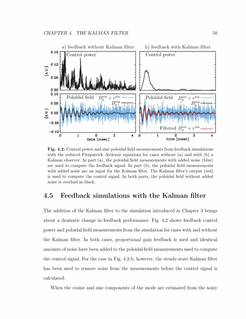
CHAPTER 4. THE KALMAN FILTER 50
Fig. 4.2: Control power and sine poloidal field measurements from feedback simulationswith the reduced Fitzpatrick–Aydemir equations for cases without (a) and with (b) aKalman observer. In part (a), the poloidal field measurements with added noise (blue)are used to compute the feedback signal. In part (b), the poloidal field measurementswith added noise are an input for the Kalman filter. The Kalman filter’s output (red)is used to compute the control signal. In both parts, the poloidal field without addednoise is overlaid in black.
4.5 Feedback simulations with the Kalman filter
The addition of the Kalman filter to the simulation introduced in Chapter 3 brings
about a dramatic change in feedback performance. Fig. 4.2 shows feedback control
power and poloidal field measurements from the simulation for cases with and without
the Kalman filter. In both cases, proportional gain feedback is used and identical
amounts of noise have been added to the poloidal field measurements used to compute
the control signal. For the case in Fig. 4.2-b, however, the steady-state Kalman filter
has been used to remove noise from the measurements before the control signal is
calculated.
When the cosine and sine components of the mode are estimated from the noisy
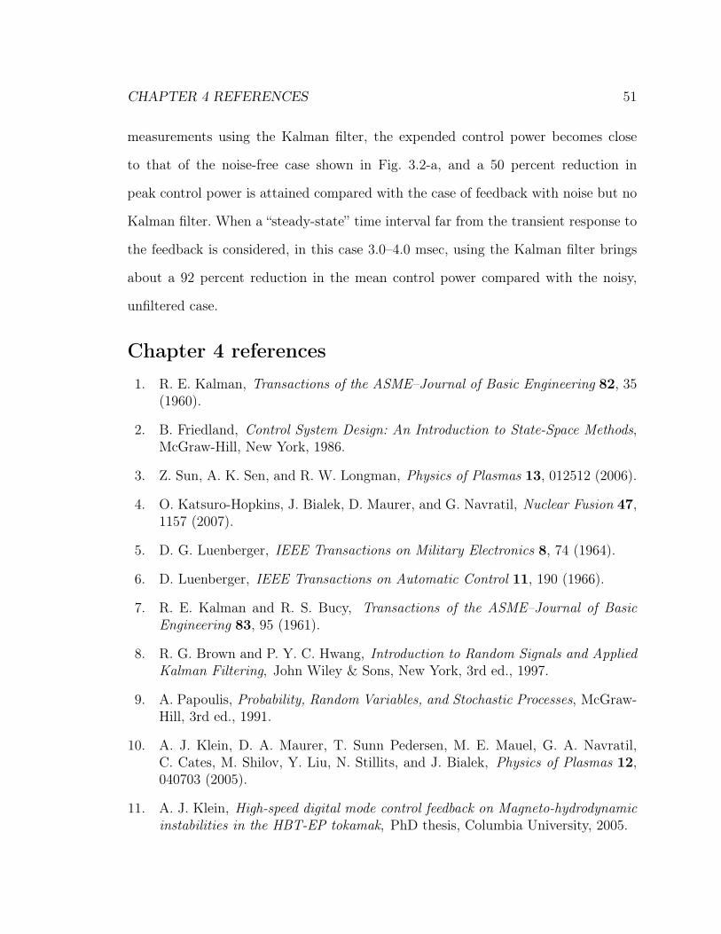
CHAPTER 4 REFERENCES 51
measurements using the Kalman filter, the expended control power becomes close
to that of the noise-free case shown in Fig. 3.2-a, and a 50 percent reduction in
peak control power is attained compared with the case of feedback with noise but no
Kalman filter. When a “steady-state” time interval far from the transient response to
the feedback is considered, in this case 3.0–4.0 msec, using the Kalman filter brings
about a 92 percent reduction in the mean control power compared with the noisy,
unfiltered case.
Chapter 4 references1. R. E. Kalman, Transactions of the ASME–Journal of Basic Engineering 82, 35
(1960).
2. B. Friedland, Control System Design: An Introduction to State-Space Methods,McGraw-Hill, New York, 1986.
3. Z. Sun, A. K. Sen, and R. W. Longman, Physics of Plasmas 13, 012512 (2006).
4. O. Katsuro-Hopkins, J. Bialek, D. Maurer, and G. Navratil, Nuclear Fusion 47,1157 (2007).
5. D. G. Luenberger, IEEE Transactions on Military Electronics 8, 74 (1964).
6. D. Luenberger, IEEE Transactions on Automatic Control 11, 190 (1966).
7. R. E. Kalman and R. S. Bucy, Transactions of the ASME–Journal of BasicEngineering 83, 95 (1961).
8. R. G. Brown and P. Y. C. Hwang, Introduction to Random Signals and AppliedKalman Filtering, John Wiley & Sons, New York, 3rd ed., 1997.
9. A. Papoulis, Probability, Random Variables, and Stochastic Processes, McGraw-Hill, 3rd ed., 1991.
10. A. J. Klein, D. A. Maurer, T. Sunn Pedersen, M. E. Mauel, G. A. Navratil,C. Cates, M. Shilov, Y. Liu, N. Stillits, and J. Bialek, Physics of Plasmas 12,040703 (2005).
11. A. J. Klein, High-speed digital mode control feedback on Magneto-hydrodynamicinstabilities in the HBT-EP tokamak, PhD thesis, Columbia University, 2005.

CHAPTER 4 REFERENCES 52
12. M. Mauel, J. Bialek, A. Boozer, C. Cates, R. James, O. Katsuro-Hopkins,A. Klein, Y. Liu, D. Maurer, D. Maslovsky, G. Navratil, T. Pedersen, M. Shilov,and N. Stillits, Nuclear Fusion 45, 285 (2005).

Chapter 5
Control system hardware on HBT-EP
The HBT-EP experiment is uniquely equipped to study feedback control of resistive
wall modes. A close fitting, hybrid conducting wall can be adjusted to change the
growth rate of external instabilities. Feedback experiments are performed with an
array of 20 poloidal field sensor coils and 20 pairs of radial field control coils. The
control and sensor coils are well coupled to the plasma, but only minimally coupled
with each other. Low latency field-programmable gate array controllers are used to
implement a feedback algorithm that contains spatial and temporal filtering, plus a
Kalman filter.
5.1 Adjustable wall sections
The HBT-EP experiment incorporates a segmented, close-fitting wall made from alter-
nating stainless steel and aluminum sections that can be adjusted radially to impact
the growth rate of external modes.1 The wall sections are evenly spaced around the
outboard edge of HBT-EP (see Fig. 5.1), and may be independently positioned in
the minor radial direction between 𝑟 = 15 cm and 𝑟 = 23 cm. There are 10 wall
53
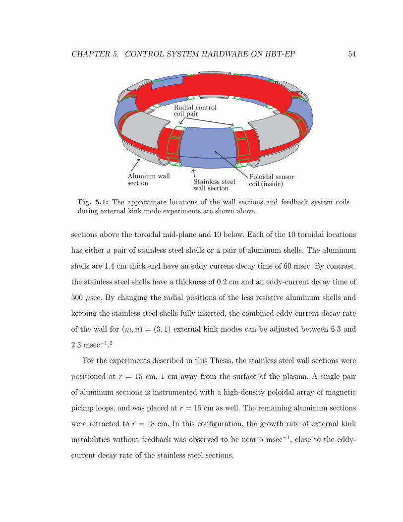
CHAPTER 5. CONTROL SYSTEM HARDWARE ON HBT-EP 54
Fig. 5.1: The approximate locations of the wall sections and feedback system coilsduring external kink mode experiments are shown above.
sections above the toroidal mid-plane and 10 below. Each of the 10 toroidal locations
has either a pair of stainless steel shells or a pair of aluminum shells. The aluminum
shells are 1.4 cm thick and have an eddy current decay time of 60 msec. By contrast,
the stainless steel shells have a thickness of 0.2 cm and an eddy-current decay time of
300 𝜇sec. By changing the radial positions of the less resistive aluminum shells and
keeping the stainless steel shells fully inserted, the combined eddy current decay rate
of the wall for (𝑚,𝑛) = (3, 1) external kink modes can be adjusted between 6.3 and
2.3 msec−1.2
For the experiments described in this Thesis, the stainless steel wall sections were
positioned at 𝑟 = 15 cm, 1 cm away from the surface of the plasma. A single pair
of aluminum sections is instrumented with a high-density poloidal array of magnetic
pickup loops, and was placed at 𝑟 = 15 cm as well. The remaining aluminum sections
were retracted to 𝑟 = 18 cm. In this configuration, the growth rate of external kink
instabilities without feedback was observed to be near 5 msec−1, close to the eddy-
current decay rate of the stainless steel sections.
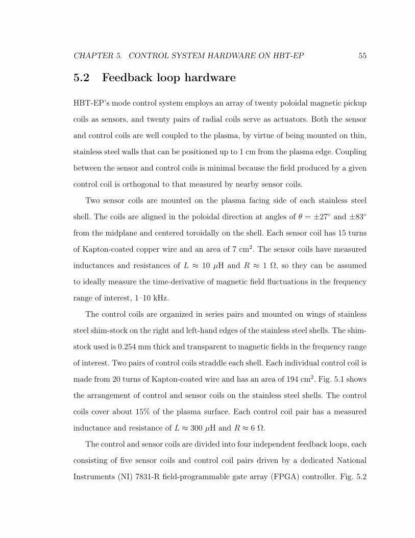
CHAPTER 5. CONTROL SYSTEM HARDWARE ON HBT-EP 55
5.2 Feedback loop hardware
HBT-EP’s mode control system employs an array of twenty poloidal magnetic pickup
coils as sensors, and twenty pairs of radial coils serve as actuators. Both the sensor
and control coils are well coupled to the plasma, by virtue of being mounted on thin,
stainless steel walls that can be positioned up to 1 cm from the plasma edge. Coupling
between the sensor and control coils is minimal because the field produced by a given
control coil is orthogonal to that measured by nearby sensor coils.
Two sensor coils are mounted on the plasma facing side of each stainless steel
shell. The coils are aligned in the poloidal direction at angles of 𝜃 = ±27∘ and ±83∘
from the midplane and centered toroidally on the shell. Each sensor coil has 15 turns
of Kapton-coated copper wire and an area of 7 cm2. The sensor coils have measured
inductances and resistances of 𝐿 ≈ 10 𝜇H and 𝑅 ≈ 1 Ω, so they can be assumed
to ideally measure the time-derivative of magnetic field fluctuations in the frequency
range of interest, 1–10 kHz.
The control coils are organized in series pairs and mounted on wings of stainless
steel shim-stock on the right and left-hand edges of the stainless steel shells. The shim-
stock used is 0.254 mm thick and transparent to magnetic fields in the frequency range
of interest. Two pairs of control coils straddle each shell. Each individual control coil is
made from 20 turns of Kapton-coated wire and has an area of 194 cm2. Fig. 5.1 shows
the arrangement of control and sensor coils on the stainless steel shells. The control
coils cover about 15% of the plasma surface. Each control coil pair has a measured
inductance and resistance of 𝐿 ≈ 300 𝜇H and 𝑅 ≈ 6 Ω.
The control and sensor coils are divided into four independent feedback loops, each
consisting of five sensor coils and control coil pairs driven by a dedicated National
Instruments (NI) 7831-R field-programmable gate array (FPGA) controller. Fig. 5.2
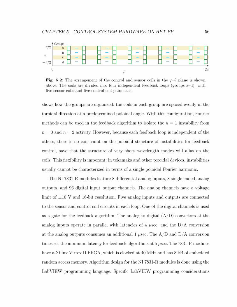
CHAPTER 5. CONTROL SYSTEM HARDWARE ON HBT-EP 56
Fig. 5.2: The arrangement of the control and sensor coils in the 𝜙–𝜃 plane is shownabove. The coils are divided into four independent feedback loops (groups a–d), withfive sensor coils and five control coil pairs each.
shows how the groups are organized: the coils in each group are spaced evenly in the
toroidal direction at a predetermined poloidal angle. With this configuration, Fourier
methods can be used in the feedback algorithm to isolate the 𝑛 = 1 instability from
𝑛 = 0 and 𝑛 = 2 activity. However, because each feedback loop is independent of the
others, there is no constraint on the poloidal structure of instabilities for feedback
control, save that the structure of very short wavelength modes will alias on the
coils. This flexibility is imporant: in tokamaks and other toroidal devices, instabilities
usually cannot be characterized in terms of a single poloidal Fourier harmonic.
The NI 7831-R modules feature 8 differential analog inputs, 8 single-ended analog
outputs, and 96 digital input–output channels. The analog channels have a voltage
limit of ±10 V and 16-bit resolution. Five analog inputs and outputs are connected
to the sensor and control coil circuits in each loop. One of the digital channels is used
as a gate for the feedback algorithm. The analog to digital (A/D) convertors at the
analog inputs operate in parallel with latencies of 4 𝜇sec, and the D/A conversion
at the analog outputs consumes an additional 1 𝜇sec. The A/D and D/A conversion
times set the minimum latency for feedback algorithms at 5 𝜇sec. The 7831-R modules
have a Xilinx Virtex II FPGA, which is clocked at 40 MHz and has 8 kB of embedded
random access memory. Algorithm design for the NI 7831-R modules is done using the
LabVIEW programming language. Specific LabVIEW programming considerations
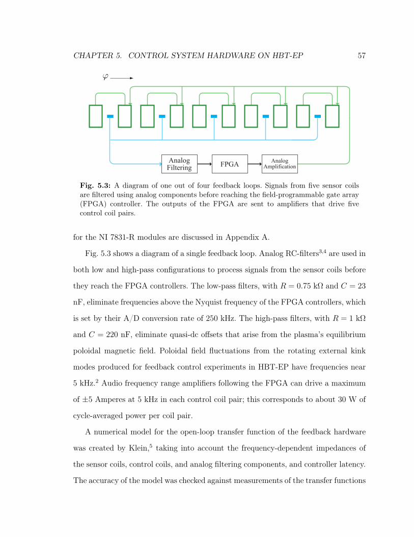
CHAPTER 5. CONTROL SYSTEM HARDWARE ON HBT-EP 57
Analog Filtering
FPGAAnalog
Amplification
! !
Fig. 5.3: A diagram of one out of four feedback loops. Signals from five sensor coilsare filtered using analog components before reaching the field-programmable gate array(FPGA) controller. The outputs of the FPGA are sent to amplifiers that drive fivecontrol coil pairs.
for the NI 7831-R modules are discussed in Appendix A.
Fig. 5.3 shows a diagram of a single feedback loop. Analog RC-filters3,4 are used in
both low and high-pass configurations to process signals from the sensor coils before
they reach the FPGA controllers. The low-pass filters, with 𝑅 = 0.75 kΩ and 𝐶 = 23
nF, eliminate frequencies above the Nyquist frequency of the FPGA controllers, which
is set by their A/D conversion rate of 250 kHz. The high-pass filters, with 𝑅 = 1 kΩ
and 𝐶 = 220 nF, eliminate quasi-dc offsets that arise from the plasma’s equilibrium
poloidal magnetic field. Poloidal field fluctuations from the rotating external kink
modes produced for feedback control experiments in HBT-EP have frequencies near
5 kHz.2 Audio frequency range amplifiers following the FPGA can drive a maximum
of ±5 Amperes at 5 kHz in each control coil pair; this corresponds to about 30 W of
cycle-averaged power per coil pair.
A numerical model for the open-loop transfer function of the feedback hardware
was created by Klein,5 taking into account the frequency-dependent impedances of
the sensor coils, control coils, and analog filtering components, and controller latency.
The accuracy of the model was checked against measurements of the transfer functions

CHAPTER 5. CONTROL SYSTEM HARDWARE ON HBT-EP 58
Fig. 5.4: Aggregate frequency-dependent amplitude and phase transfer functions for allcomponents in the feedback loop. The red, dashed lines show the uncorrected transferfunction. Solid, blue lines show the transfer function when corrected by the phase-lagand phase-lead temporal filters in the feedback algorithm.5
of each component in the loop, and Klein added a second-order, lead–lag temporal
filter to the FPGA algorithm to optimize the transfer function for a flat amplitude and
phase response in the 1–10 kHz range. Figure 5.4 shows the model of the total transfer
function before and after this optimization. The large change in the uncorrected phase
transfer between 1–10 kHz could impair the ability to do feedback. For example, the
uncorrected phase transfer at 1.5 kHz is about 𝜋/4 rad. It is possible to do negative
feedback on a mode rotating at this frequency by adjusting the toroidal phasing of
the control signals (see Eq. 5.2). However, any activity at frequencies near 7 kHz has
a phase transfer of −𝜋/4 rad, and will be phased to excite, rather than suppress, the
1.5 kHz instability.
Experiments that measured the response of an unstable external kink mode to
feedback applied with different temporal filters demonstrated the importance of com-
pensating for the open-loop transfer function properly: feedback with the filter that
resulted in the smallest amount frequency-dependent amplitude and phase variation
in the combined transfer function was the most successful at suppressing the external
kink instability.2
CHAPTER 5. CONTROL SYSTEM HARDWARE ON HBT-EP 59
5.3 Feedback algorithm
For initial experiments performed by Klein,2 an algorithm with spatial and temporal
filtering was implemented on the FPGA controllers. These filters are retained for use in
the present algorithm. The Kalman filter described in Section 4.4 is also included. This
Section provides an overview of the feedback algorithm. A more detailed description
is given in Appendix B.
The spatial filter uses a discrete Fourier transform (DFT) to separate a toroidal
𝑛 = 1 mode from any 𝑛 = 0 and 𝑛 = 2 activity in a group of five sensor inputs
𝑠1, . . . , 𝑠5, giving the cosine and sine components of the poloidal field fluctuations,
⎛⎜⎝𝐵cosp
𝐵sinp
⎞⎟⎠ = 𝐷𝑛=1
⎛⎜⎜⎜⎜⎝𝑠1
...
𝑠5
⎞⎟⎟⎟⎟⎠ . (5.1)
The inverse DFT is used in conjunction with a rotation operator 𝑅Δ𝜙fthat adjusts
the toroidal phasing of feedback about a predetermined angle ∆𝜙f and a proportional
gain matrix 𝐺 to compute the control coil outputs 𝑐1, . . . , 𝑐5 in the final stage of the
algorithm, ⎛⎜⎜⎜⎜⎝𝑐1...
𝑐5
⎞⎟⎟⎟⎟⎠ = 𝐷−1𝑛=1𝑅Δ𝜙f
𝐺
⎛⎜⎝𝐵cosp
𝐵sinp
⎞⎟⎠ . (5.2)
The matrices 𝐷𝑛=1 and 𝐷−1𝑛=1𝑅Δ𝜙f
𝐺 are calculated prior to run time and stored in
memory on the NI 7831-R modules.
The second order phase-lag, phase-lead temporal filter used previously2 is broken
CHAPTER 5. CONTROL SYSTEM HARDWARE ON HBT-EP 60
into two first order filters, each of the form
𝑦𝑘 = 𝑎0𝑥𝑘 + 𝑎1𝑥𝑘−1 + 𝑏1𝑦𝑘−1.
Here, the filtered output 𝑦 at time step 𝑘 is given in terms of an input 𝑥𝑘 and the
value of the filter’s input and output at the previous time step. The coefficients 𝑎0,
𝑎1, and 𝑏1 are chosen to provide the correction to the system transfer function shown
in Fig. 5.4
The Kalman filter is implemented using the steady-state limit described in Section
4.3; that is, the filter’s estimate ˆ𝑥 is given by
ˆ𝑥𝑘 = Φˆ𝑥𝑘−1 +𝐾𝑘. (5.3)
The matrices Φ and 𝐾 (defined in Eqs. 4.19 and 4.20) are calculated prior to run
time and stored in memory on the NI 7831-R controllers, leaving only Eq. 5.3 to be
solved by the feedback algorithm.
The Kalman filter is sandwiched between the phase-lag and phase-lead portions of
the temporal filter (see Fig. 5.5). The lag compensator has a large amount of integral
action and corrects for the transfer functions of the nearly-ideal magnetic pickup coils
used as sensors and of analog filtering components on the input leg of the feedback
loop. The lead compensator follows the Kalman filter and corrects for the integrating
nature of the control coils. Together, the temporal filters insure that the Kalman filter
sees a signal that is proportional to the perturbed magnetic field (and not, say, its
time derivative), and that the field applied by the control coils will be proportional
to the Kalman filter’s estimate when the feedback loop is closed. That is, the Kalman
filter is designed to use a measurement with units of magnetic field to produce a

CHAPTER 5. CONTROL SYSTEM HARDWARE ON HBT-EP 61
Fig. 5.5: A diagram showing the stages of the feedback algorithm. The 𝑛 = 1 modeis computed from a group of five sensor coils using a DFT and optionally mixed witha noise input. The phase-lag, Kalman, and phase-lead filters are then applied, followedby the proportional gain, toroidal rotation, and inverse DFT operators.
refined estimate of that field.
Additionally, the capacity of this Kalman filter to produce estimates of the ampli-
tude and phase of a rotating, growing 𝑛 = 1 mode makes it ideally suited to operate
on the Fourier domain of the spatial DFT. The temporal filters are placed inside the
forward and inverse DFT operations simply because the DFT step brings about a
reduction in the number of signals that must be filtered, allowing for the algorithm
to be implemented using fewer arithmetical operations.
Two additional capabilities are useful for comparing algorithms in experiments.
First, the Kalman filter stage of the algorithm can be bypassed, resulting in a conven-
tional algorithm that is identical to that used in earlier experiments.2,5 Figure 5.6-a
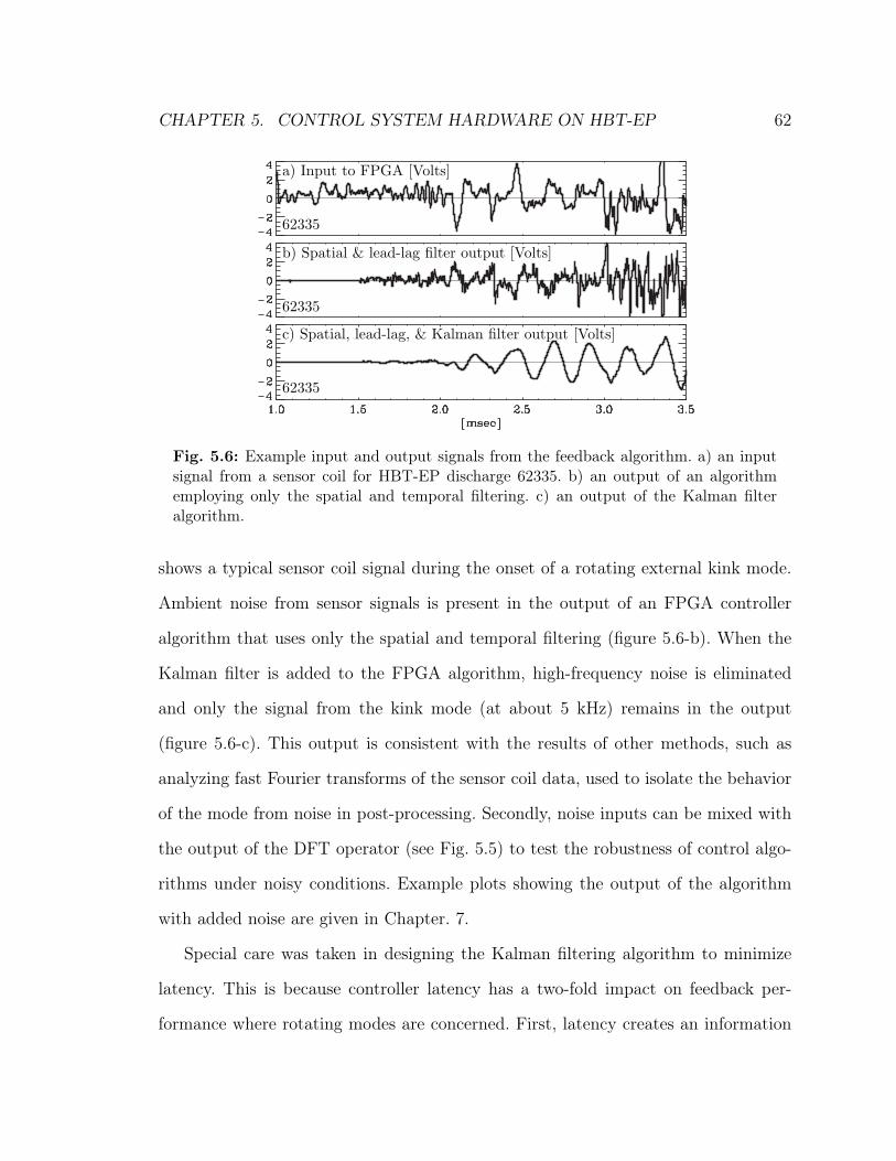
CHAPTER 5. CONTROL SYSTEM HARDWARE ON HBT-EP 62
Fig. 5.6: Example input and output signals from the feedback algorithm. a) an inputsignal from a sensor coil for HBT-EP discharge 62335. b) an output of an algorithmemploying only the spatial and temporal filtering. c) an output of the Kalman filteralgorithm.
shows a typical sensor coil signal during the onset of a rotating external kink mode.
Ambient noise from sensor signals is present in the output of an FPGA controller
algorithm that uses only the spatial and temporal filtering (figure 5.6-b). When the
Kalman filter is added to the FPGA algorithm, high-frequency noise is eliminated
and only the signal from the kink mode (at about 5 kHz) remains in the output
(figure 5.6-c). This output is consistent with the results of other methods, such as
analyzing fast Fourier transforms of the sensor coil data, used to isolate the behavior
of the mode from noise in post-processing. Secondly, noise inputs can be mixed with
the output of the DFT operator (see Fig. 5.5) to test the robustness of control algo-
rithms under noisy conditions. Example plots showing the output of the algorithm
with added noise are given in Chapter. 7.
Special care was taken in designing the Kalman filtering algorithm to minimize
latency. This is because controller latency has a two-fold impact on feedback per-
formance where rotating modes are concerned. First, latency creates an information
CHAPTER 5 REFERENCES 63
delay between the plasma and controller; the controller must be fast enough to keep
pace with changes in the plasma equilibrium and quickly growing modes. Secondly,
latency impacts the system transfer function by adding a phase-shift that is linear
in frequency. In the case of HBT-EP, controller latencies greater than 30 𝜇sec create
sufficient phase shift (even with digital compensation) to allow for the possibility of
the feedback suppressing a low-frequency instability while simultaneously exciting a
high-frequency one.
Chapter 5 references1. A. Garofalo, E. Eisner, T. Ivers, R. Kombargi, M. Mauel, D. Maurer, D. Nadle,
G. Navratil, M. V. Sankar, E. Taylor, and Q. Xiao, Nuclear Fusion 38, 1029(1998).
2. A. J. Klein, D. A. Maurer, T. Sunn Pedersen, M. E. Mauel, G. A. Navratil,C. Cates, M. Shilov, Y. Liu, N. Stillits, and J. Bialek, Physics of Plasmas 12,040703 (2005).
3. J. C. Sprott, Introduction to Modern Electronics, John Wiley & Sons, NewYork, 1981.
4. P. Horowitz and W. Hill, The Art of Electronics, Cambridge University Press,Cambridge, UK, 2nd ed., 1989.
5. A. J. Klein, High-speed digital mode control feedback on Magneto-hydrodynamicinstabilities in the HBT-EP tokamak, PhD thesis, Columbia University, 2005.

Chapter 6
Observation of external kink mode
activity
External kink instabilities are created in HBT-EP discharges by establishing a gra-
dient in the current density profile near the edge of the plasma. In this Chapter, the
programming of external kink unstable discharges is discussed in detail, and poloidal
magnetic field fluctuations from an example discharge are examined. Two analysis
techniques, a spatial Fourier transform and the biorthogonal decomposition, are used
to analyze data from multiple poloidal field sensor coils and provide information about
the structure and evolution of the instability.
6.1 Discharge programming
In HBT-EP, tokamak plasma discharges are produced and sustained through careful
programming of current waveforms in the Ohmic heating (OH), vertial field (VF),
and toroidal field (TF) coils. The coils are powered by ignitron-switched capacitor
banks, and the operator specifies the charging voltage for each bank as a means of
64
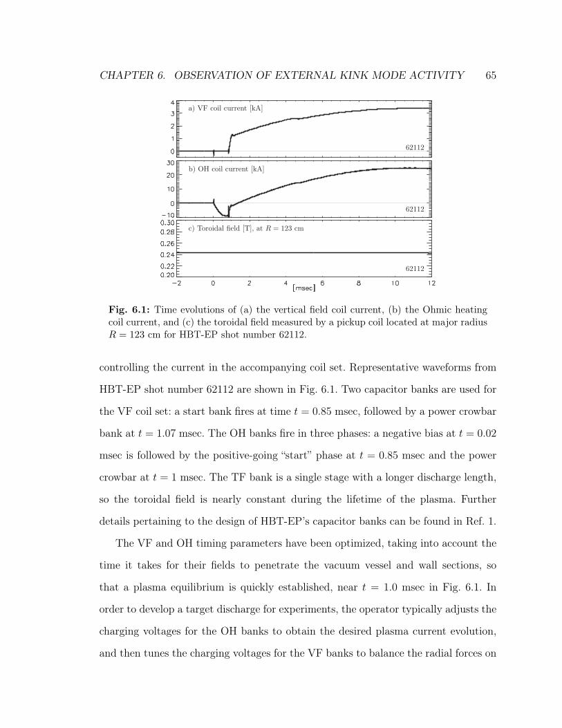
CHAPTER 6. OBSERVATION OF EXTERNAL KINK MODE ACTIVITY 65
Fig. 6.1: Time evolutions of (a) the vertical field coil current, (b) the Ohmic heatingcoil current, and (c) the toroidal field measured by a pickup coil located at major radius𝑅 = 123 cm for HBT-EP shot number 62112.
controlling the current in the accompanying coil set. Representative waveforms from
HBT-EP shot number 62112 are shown in Fig. 6.1. Two capacitor banks are used for
the VF coil set: a start bank fires at time 𝑡 = 0.85 msec, followed by a power crowbar
bank at 𝑡 = 1.07 msec. The OH banks fire in three phases: a negative bias at 𝑡 = 0.02
msec is followed by the positive-going “start” phase at 𝑡 = 0.85 msec and the power
crowbar at 𝑡 = 1 msec. The TF bank is a single stage with a longer discharge length,
so the toroidal field is nearly constant during the lifetime of the plasma. Further
details pertaining to the design of HBT-EP’s capacitor banks can be found in Ref. 1.
The VF and OH timing parameters have been optimized, taking into account the
time it takes for their fields to penetrate the vacuum vessel and wall sections, so
that a plasma equilibrium is quickly established, near 𝑡 = 1.0 msec in Fig. 6.1. In
order to develop a target discharge for experiments, the operator typically adjusts the
charging voltages for the OH banks to obtain the desired plasma current evolution,
and then tunes the charging voltages for the VF banks to balance the radial forces on

CHAPTER 6. OBSERVATION OF EXTERNAL KINK MODE ACTIVITY 66
Fig. 6.2: Time evolutions of the (a) plasma current, (b) plasma major radius, (c) plasmaminor radius, and (d) edge safety factor for HBT-EP discharge 62112.
the plasma. The VF coils also drive a small amount of plasma current, so the process
of tuning bank voltages is usually iterative.
External kink unstable discharges are created by ramping the plasma current 𝐼p,
as is shown in Fig. 6.2-a. In this discharge, the plasma current is ramped at ∼3
MA/sec. At this rate, current density is added at the plasma edge more quickly than
it can diffuse inward, resulting in a broad current density profile with a large gradient
near the plasma edge. Current density gradients are a source of free energy that can
drive external kink instabilities (see the discussion in Section 2.4).
The plasma’s major radius 𝑅0 (Fig. 6.2-b) is calculated using the signal from a
poloidal Rogowski coil2 with a winding density proportional to cos 𝜃. Corrections are
included for pickup in the Rogowski coil from the VF and OH fields. The plasma

CHAPTER 6. OBSERVATION OF EXTERNAL KINK MODE ACTIVITY 67
Fig. 6.3: Time evolution (a) and frequency spectrum amplitude (b) of poloidal fieldfluctuations measured by a feedback system sensor coil. The frequency spectrum iscomputed over the highlighted time-window, 1.8–2.8 msec.
minor radius 𝑎 (Fig. 6.2-c) is then obtained from the minimum distance between 𝑅0
and the locations of four fixed plasma limiter blades: inboard, outboard, upper, and
lower. The safety factor at the edge of the plasma (Fig. 6.2-d) is obtained using the
high aspect ratio approximation3
𝑞𝑎 =𝑎𝐵t(𝑅0)
𝑅0𝐵p
, (6.1)
with the equilibrium poloidal field 𝐵p ≈ 𝜇0𝐼p/2𝜋𝑎. The toroidal field on axis 𝐵t(𝑅0)
is estimated from the value measured at 𝑅 = 123 cm by assuming a 1/𝑅 dependence.
A numerical equilibrium reconstruction and MHD stability analysis was performed
by Klein4 for a discharge created in the same fashion as shot 62112. This analysis
yielded a negative value of 𝛿𝑊 for a mode with an (𝑚,𝑛) = (3, 1) helicity. If 𝛿𝑊 < 0
for a given perturbation, the plasma is linearly MHD unstable to that perturba-
tion (see Eq. 2.13). A calculation of the normalized stability parameters 𝑠 and 𝑠crit
(discussed in Section 3.1) showed that 𝑠 ≈ 𝑠crit for this instability, indicating that
the quickly growing, ideal external kink branch of the RWM dispersion relation5–7 is
unstable.

CHAPTER 6. OBSERVATION OF EXTERNAL KINK MODE ACTIVITY 68
In ideal MHD theory, the value of the edge safety factor plays an important role
in determining the stability of external modes. In particular, the ideal external kink
is expected to be unstable when 𝑞𝑎 is slightly below a rational number, that is, when
a rational surface lies just outside the plasma edge.8 Fig. 6.3-a shows poloidal field
fluctuations measured by one of HBT-EP’s feedback sensor coils for shot 62112. Dur-
ing the time window when 𝑞𝑎 < 3, about 1.8–2.8 msec, the poloidal field fluctuations
measured by the sensor coil are consistent with those of an instability rotating at
3–4 kHz. The amplitude of the frequency spectrum of these oscillations is shown in
Fig. 6.3-b. Analysis methods that combine information from more than one sensor
coil (described in the next Section) can be used to determine the spatial structure of
the instability.
6.2 Analysis of magnetic fluctuations
In total, about 36 independent point measurements of poloidal magnetic field fluc-
tuations in HBT-EP are available. The poloidal field coils are mounted on the wall
sections described in Chapter 5. There are several ways to combine these measure-
ments to obtain a global view of the fluctuations. In the first method described here,
signals from the feedback system sensors are Fourier analyzed to obtain a toroidal
mode number. The second method involves using a singular value decomposition to
analyze all the measurements at once. The results of both techniques show a dominant
(𝑚,𝑛) = (3, 1) instability for HBT-EP shot 62112.
6.2.1 Fourier analysis
Because the feedback system sensor coils are arranged in groups of five coils evenly
spaced in the toroidal direction (see, for example, Figs. 5.1 and 5.2), signals from each

CHAPTER 6. OBSERVATION OF EXTERNAL KINK MODE ACTIVITY 69
Fig. 6.4: Spatial Fourier spectrum amplitudes calculated from poloidal field sensorfluctuations for HBT-EP discharge 62112. The colors denote poloidal groupings of fivesensors each. The highlighted region marks the time window when 𝑞𝑎 < 3.
group can be Fourier analyzed to determine the toroidal mode number 𝑛 of poloidal
field fluctuations for 𝑛 = 0, 1, and 2. A discrete Fourier transform is performed on
each group of poloidal field fluctuation measurements at every time step. Then, a
time-dependent amplitude and phase can be calculated for each 𝑛-number and coil
group. Fig. 6.4 shows the amplitude results for each group, organized by 𝑛-number
for shot 62112. During the 1.8–2.8 msec time window in which the plasma is external
kink mode unstable, small amount of activity is detected in the 𝑛 = 0 and 𝑛 = 2
harmonics. The 𝑛 = 1 harmonic, however, shows an exponentially growing mode in all
four sensor groups, indicating that the instability has an odd toroidal mode number.*
The time-dependent phase for the 𝑛 = 1 mode is shown for each sensor coil group*Toroidal mode numbers greater than 𝑛 = 2 cannot be detected using five evenly spaced mea-
surements, leaving open the possibility that the 𝑛 = 1 signal could be created by a higher order oddharmonic aliasing on the coils. However, the energy required to apply a harmonic perturbation to aplasma increases with the square of 𝑛. This can be seen be evaluating the first term in Eq. 2.17 fora perturbation of the form 𝜉 = 𝜉0 exp(𝑖𝑛𝜙). Thus, the mode is most likely 𝑛 = 1.

CHAPTER 6. OBSERVATION OF EXTERNAL KINK MODE ACTIVITY 70
Fig. 6.5: Spatial Fourier spectrum phase for the 𝑛 = 1 mode for HBT-EP shot 62112.The colors of the traces denote individual sensor groups as in Fig. 6.4. The highlightedregion marks the time when 𝑞𝑎 < 3.
in Fig. 6.5. As the mode develops, the phases are seen to increase linearly in time
and then jump from 𝜋 to −𝜋 rad at regular intervals, indicating that the 𝑛 = 1 mode
is rotating. During this time, about 2.0–2.8 msec, signals from poloidally adjacent
groups are out of phase by about 𝜋 rad, and signals from alternating groups are
in phase. This pattern is consistent with that of an instability with poloidal mode
number 𝑚 = 3, Thus, we can identify the helicity of the mode as (𝑚,𝑛) = (3, 1). The
instability is resonant with the 𝑞 = 3/1 magnetic surface, which (by the evolution of
𝑞𝑎 shown in Fig. 6.2–d) is just outside the plasma edge. Therefore, it is an external
mode.
6.2.2 Biorthogonal decomposition analysis
In addition to the feedback system sensor coils, HBT-EP is equipped with a high
density poloidal array of 16 poloidal field pickup coils. The positions of all the coils
are overlaid in Figs. 6.7 and 6.8. All the stainless steel wall sections plus the alu-
minum wall sections on which the poloidal array is mounted were fully inserted for
the external kink mode experiments described here, providing a total of 34 poloidal
field measurements at the same minor radius. (Two coils were inoperable at the time
of this work.) Because the coils are not evenly spaced, they cannot be analyzed in
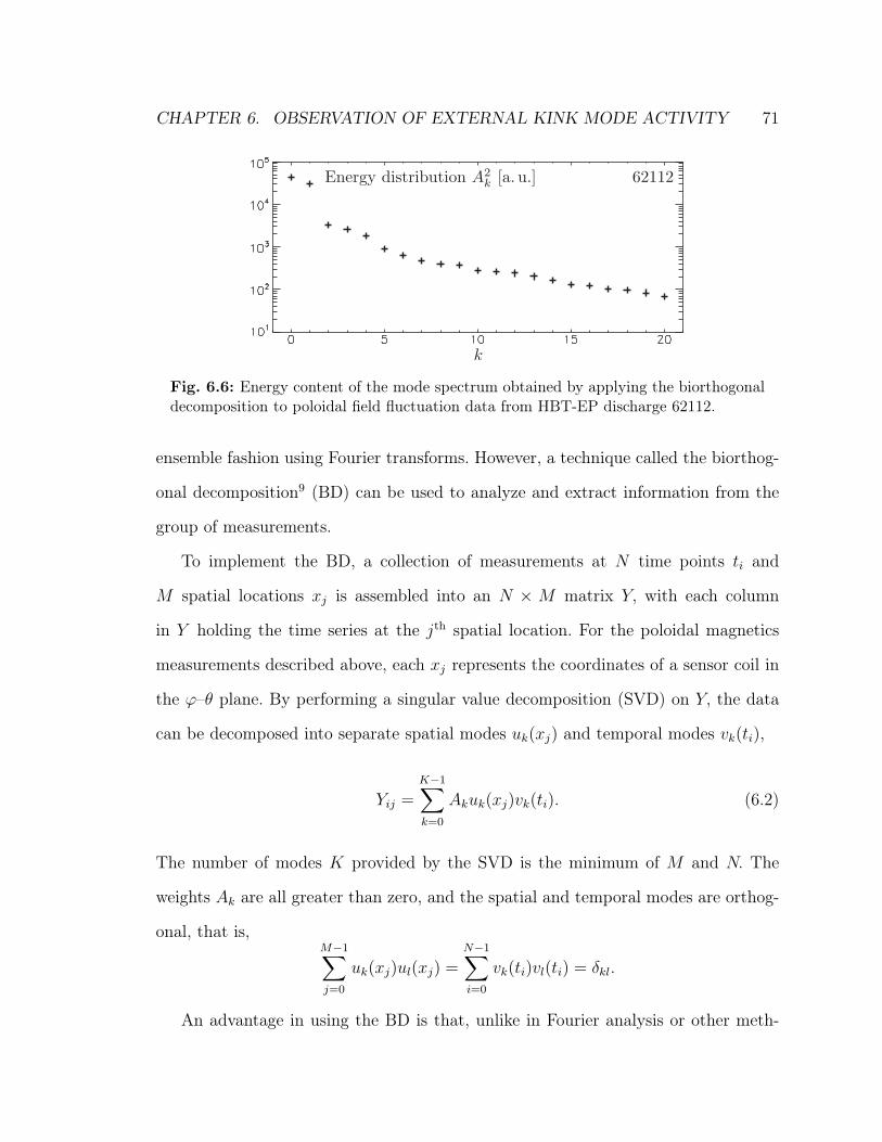
CHAPTER 6. OBSERVATION OF EXTERNAL KINK MODE ACTIVITY 71
Fig. 6.6: Energy content of the mode spectrum obtained by applying the biorthogonaldecomposition to poloidal field fluctuation data from HBT-EP discharge 62112.
ensemble fashion using Fourier transforms. However, a technique called the biorthog-
onal decomposition9 (BD) can be used to analyze and extract information from the
group of measurements.
To implement the BD, a collection of measurements at 𝑁 time points 𝑡𝑖 and
𝑀 spatial locations 𝑥𝑗 is assembled into an 𝑁 × 𝑀 matrix 𝑌, with each column
in 𝑌 holding the time series at the 𝑗th spatial location. For the poloidal magnetics
measurements described above, each 𝑥𝑗 represents the coordinates of a sensor coil in
the 𝜙–𝜃 plane. By performing a singular value decomposition (SVD) on 𝑌, the data
can be decomposed into separate spatial modes 𝑢𝑘(𝑥𝑗) and temporal modes 𝑣𝑘(𝑡𝑖),
𝑌𝑖𝑗 =𝐾−1∑𝑘=0
𝐴𝑘𝑢𝑘(𝑥𝑗)𝑣𝑘(𝑡𝑖). (6.2)
The number of modes 𝐾 provided by the SVD is the minimum of 𝑀 and 𝑁. The
weights 𝐴𝑘 are all greater than zero, and the spatial and temporal modes are orthog-
onal, that is,𝑀−1∑𝑗=0
𝑢𝑘(𝑥𝑗)𝑢𝑙(𝑥𝑗) =𝑁−1∑𝑖=0
𝑣𝑘(𝑡𝑖)𝑣𝑙(𝑡𝑖) = 𝛿𝑘𝑙.
An advantage in using the BD is that, unlike in Fourier analysis or other meth-

CHAPTER 6. OBSERVATION OF EXTERNAL KINK MODE ACTIVITY 72
Fig. 6.7: The first pair of spatial modes obtained using a biorthogonal decompositionanalysis of poloidal field fluctuations from HBT-EP discharge 62112. The peak amplitudeof the modes is normalized to 1.0.
ods of fitting data to prescribed functions, nothing is assumed about the spatial or
temporal structure of the data. The BD naturally reveals orthogonal sets of modes
that describe what is measured. However, it can be difficult to interpret or assign a
physical meaning to the modes.
The squares of the weights are interpreted as the amount of “energy” in each mode.
Fig. 6.6 shows the energy of the first 20 modes from a BD analysis of the poloidal
magnetics for HBT-EP shot 62112 over the time window 1.8–2.8 msec. For this data
set, modes 𝑘 = 0 and 𝑘 = 1 represent about 85% of the total energy, and the next
pair of modes represents 6%.
It is interesting that a pair of modes is set apart from the rest by about an order
of magnitude in energy. The corresponding spatial structures, 𝑢0(𝑥) and 𝑢1(𝑥), are
pictured in Fig. 6.7. The spatial mode plots were made by positioning each 𝑢(𝑥𝑗) in
the 𝜙–𝜃 plane and interpolating the data between measurement points. The structures
shown in Fig. 6.7 are quite similar: when the amplitude is considered along a line of
constant 𝜃, the toroidal wave number can clearly be identified as 𝑛 = 1 in each.
Looking along a line of constant 𝜙, there are about 1.5 wavelengths in a 180∘ poloidal

CHAPTER 6. OBSERVATION OF EXTERNAL KINK MODE ACTIVITY 73
Fig. 6.8: The second pair of spatial modes obtained using a biorthogonal decompositionanalysis of poloidal field fluctuations from HBT-EP discharge 62112. The peak amplitudeof the modes is normalized to 1.0.
span, consistent with 𝑚 = 3. These two spatial modes are roughly identical to within
a phase-shift of a quarter wavelength in either 𝜃 or 𝜑. Therefore, the 𝑢0 and 𝑢1 modes
can be interpreted as if they were a cosine–sine quadrature pair.
Spatial modes 𝑢2 and 𝑢3 are shown in Fig. 6.8. Their structure is more difficult to
interpret, but a toroidal mode number 𝑛 = 2 can clearly be identified. There is little
variation in the poloidal direction, except for at the right-hand edge of each contour
plot, where the sampling density is higher. At the right-hand edge, there are three
wavelengths over a span of 180∘ in the 𝜃-direction, consistent with 𝑚 = 6. So, we
can interpret the second pair of modes as an (𝑚,𝑛) = (6, 2) cosine–sine pair that is
aliased in areas where the coil coverage is not dense enough to resolve 𝑚 = 6.
Time histories of the first four temporal modes are shown in Fig. 6.9. The modes
are multiplied by their respective weights so that the most significant modes stand
out. The 𝑣0 and 𝑣1 modes clearly form a quadrature pair for a instability rotating at
about 3–4 kHz. The relationship between 𝑣3 and 𝑣4 is less obvious; the phase-shift
between them changes in time.
The spatial and temporal modes corresponding to 𝑘 > 3 represent about 9% of the

CHAPTER 6 REFERENCES 74
Fig. 6.9: Time histories of the first four temporal modes obtained using a biorthogonaldecomposition analysis of poloidal field fluctuations from HBT-EP discharge 62112.
energy in the spectrum, combined. These modes have high or broadband temporal
frequencies and unusual spatial structures. They are difficult to interpret physically,
and do not always occur in quadrature pairs. The modes may arise from signal noise
or calibration errors in the poloidal field measurements.
The results of the BD analysis of the ensemble of 34 poloidal field measurements
confirm the main conclusion drawn from the Fourier analysis of the feedback system
sensor coil groups by themselves: that the instability observed during the time window
1.8–2.8 msec in HBT-EP discharge 62112 is an (𝑚,𝑛) = (3, 1) mode, rotating near 3–4
kHz. In addition, the BD results show some evidence of low-amplitude (𝑚,𝑛) = (6, 2)
activity.
Chapter 6 references1. D. A. Gates, Passive Stabilization of MHD Instabilities at High 𝛽N in the HBT-
EP Tokamak, PhD thesis, Columbia University, 1993.
2. I. H. Hutchinson, Principles of Plasma Diagnostics, Cambridge University Press,Cambridge, UK, 2nd ed., 2002.
3. J. Wesson, Tokamaks, Oxford University Press, New York, 3rd ed., 2004.
4. A. J. Klein, High-speed digital mode control feedback on Magneto-hydrodynamicinstabilities in the HBT-EP tokamak, PhD thesis, Columbia University, 2005.
CHAPTER 6 REFERENCES 75
5. A. Bondeson and D. J. Ward, Phys. Rev. Lett. 72, 2709 (1994).
6. R. Betti and J. P. Freidberg, Phys. Rev. Lett. 74, 2949 (1995).
7. M. Chu, J. Greene, T. Jensen, R. Miller, A. Bondeson, R. Johnson, and M. Mauel,Physics of Plasmas 2, 2236 (1995).
8. V. D. Shafranov, Soviet Physics – Technical Physics 15, 175 (1970).
9. T. D. de Wit, A.-L. Pecquet, J.-C. Vallet, and R. Lima, Physics of Plasmas 1,3288 (1994).
Chapter 7
Closed loop Kalman filter
experiments
The most important tests of the Kalman filter algorithm presented in Chapter 5 are
in experiments with external kink mode-unstable plasmas. The experimental results
presented in this Chapter show clear enhancements in feedback performance when the
Kalman filter is used. In particular, feedback with the Kalman filter remains effective
even when large amounts of noise are added to input signals. The results of feedback
experiments that investigated the impact of various algorithm parameter settings are
described here as well. The spatial phasing between the feedback and the instability
was investigated, as well as the Kalman filter’s growth rate, rotation rate, and noise
covariance parameters. Feedback performance was improved when optimal values for
these parameters were used.
76
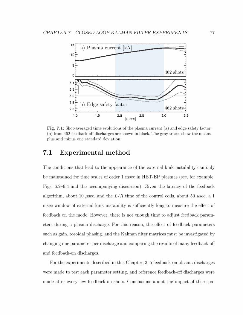
CHAPTER 7. CLOSED LOOP KALMAN FILTER EXPERIMENTS 77
Fig. 7.1: Shot-averaged time evolutions of the plasma current (a) and edge safety factor(b) from 462 feedback-off discharges are shown in black. The gray traces show the meansplus and minus one standard deviation.
7.1 Experimental method
The conditions that lead to the appearance of the external kink instability can only
be maintained for time scales of order 1 msec in HBT-EP plasmas (see, for example,
Figs. 6.2–6.4 and the accompanying discussion). Given the latency of the feedback
algorithm, about 10 𝜇sec, and the 𝐿/𝑅 time of the control coils, about 50 𝜇sec, a 1
msec window of external kink instability is sufficiently long to measure the effect of
feedback on the mode. However, there is not enough time to adjust feedback param-
eters during a plasma discharge. For this reason, the effect of feedback parameters
such as gain, toroidal phasing, and the Kalman filter matrices must be investigated by
changing one parameter per discharge and comparing the results of many feedback-off
and feedback-on discharges.
For the experiments described in this Chapter, 3–5 feedback-on plasma discharges
were made to test each parameter setting, and reference feedback-off discharges were
made after every few feedback-on shots. Conclusions about the impact of these pa-
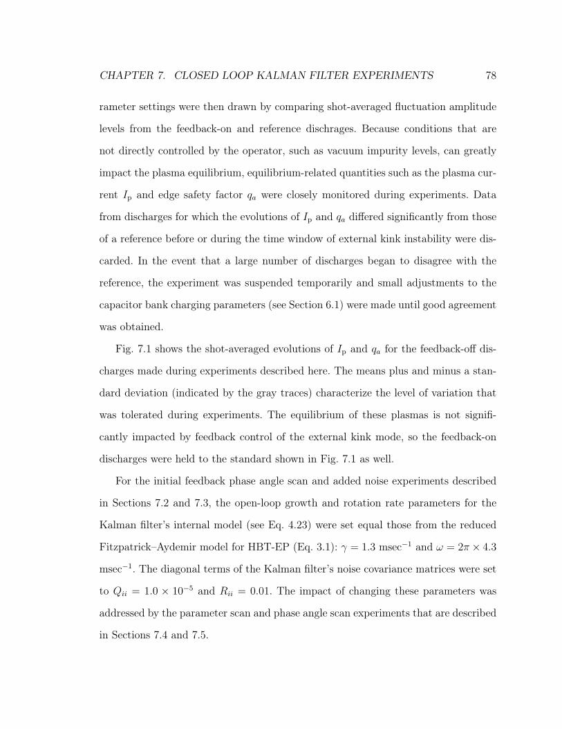
CHAPTER 7. CLOSED LOOP KALMAN FILTER EXPERIMENTS 78
rameter settings were then drawn by comparing shot-averaged fluctuation amplitude
levels from the feedback-on and reference dischrages. Because conditions that are
not directly controlled by the operator, such as vacuum impurity levels, can greatly
impact the plasma equilibrium, equilibrium-related quantities such as the plasma cur-
rent 𝐼p and edge safety factor 𝑞𝑎 were closely monitored during experiments. Data
from discharges for which the evolutions of 𝐼p and 𝑞𝑎 differed significantly from those
of a reference before or during the time window of external kink instability were dis-
carded. In the event that a large number of discharges began to disagree with the
reference, the experiment was suspended temporarily and small adjustments to the
capacitor bank charging parameters (see Section 6.1) were made until good agreement
was obtained.
Fig. 7.1 shows the shot-averaged evolutions of 𝐼p and 𝑞𝑎 for the feedback-off dis-
charges made during experiments described here. The means plus and minus a stan-
dard deviation (indicated by the gray traces) characterize the level of variation that
was tolerated during experiments. The equilibrium of these plasmas is not signifi-
cantly impacted by feedback control of the external kink mode, so the feedback-on
discharges were held to the standard shown in Fig. 7.1 as well.
For the initial feedback phase angle scan and added noise experiments described
in Sections 7.2 and 7.3, the open-loop growth and rotation rate parameters for the
Kalman filter’s internal model (see Eq. 4.23) were set equal those from the reduced
Fitzpatrick–Aydemir model for HBT-EP (Eq. 3.1): 𝛾 = 1.3 msec−1 and 𝜔 = 2𝜋 × 4.3
msec−1. The diagonal terms of the Kalman filter’s noise covariance matrices were set
to 𝑄𝑖𝑖 = 1.0 × 10⁻⁵ and 𝑅𝑖𝑖 = 0.01. The impact of changing these parameters was
addressed by the parameter scan and phase angle scan experiments that are described
in Sections 7.4 and 7.5.
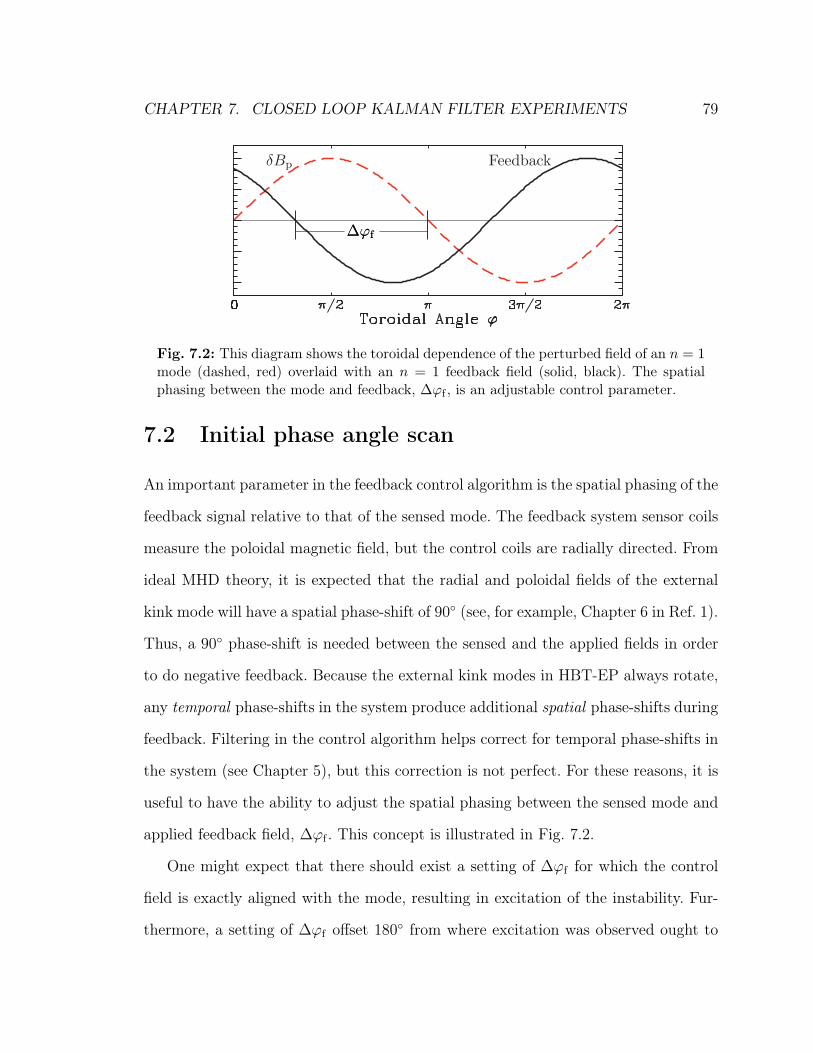
CHAPTER 7. CLOSED LOOP KALMAN FILTER EXPERIMENTS 79
Fig. 7.2: This diagram shows the toroidal dependence of the perturbed field of an 𝑛 = 1mode (dashed, red) overlaid with an 𝑛 = 1 feedback field (solid, black). The spatialphasing between the mode and feedback, Δ𝜙f , is an adjustable control parameter.
7.2 Initial phase angle scan
An important parameter in the feedback control algorithm is the spatial phasing of the
feedback signal relative to that of the sensed mode. The feedback system sensor coils
measure the poloidal magnetic field, but the control coils are radially directed. From
ideal MHD theory, it is expected that the radial and poloidal fields of the external
kink mode will have a spatial phase-shift of 90∘ (see, for example, Chapter 6 in Ref. 1).
Thus, a 90∘ phase-shift is needed between the sensed and the applied fields in order
to do negative feedback. Because the external kink modes in HBT-EP always rotate,
any temporal phase-shifts in the system produce additional spatial phase-shifts during
feedback. Filtering in the control algorithm helps correct for temporal phase-shifts in
the system (see Chapter 5), but this correction is not perfect. For these reasons, it is
useful to have the ability to adjust the spatial phasing between the sensed mode and
applied feedback field, ∆𝜙f . This concept is illustrated in Fig. 7.2.
One might expect that there should exist a setting of ∆𝜙f for which the control
field is exactly aligned with the mode, resulting in excitation of the instability. Fur-
thermore, a setting of ∆𝜙f offset 180∘ from where excitation was observed ought to

CHAPTER 7. CLOSED LOOP KALMAN FILTER EXPERIMENTS 80
Fig. 7.3: Poloidal field fluctuations measured by a sensor coil 1 cm from the plasmasurface for the case of: (a) no feedback, (b) positive feedback using the Kalman filterand (c) negative feedback with the Kalman filter.
suppress the mode’s amplitude. In initial experiments with the Kalman filter algo-
rithm, this behavior was observed as expected. In Fig. 7.3, poloidal field fluctuation
measurements from feedback with two settings of settings of ∆𝜙f are compared with
a feedback-off reference. Excitation of the fluctuations is observed for ∆𝜙f = −90∘,
and suppression is observed when ∆𝜙f = 90∘.
An optimum value for ∆𝜙f was determined by scanning this parameter through
360∘ in 10∘ increments. The contour plot in Fig. 7.4 shows the amplitude of the Fourier
spectrum of poloidal magnetic field fluctuations from this scan. The plot’s polar axis
marks the setting of ∆𝜙f , and the radial axis marks the frequency of the spectrum.
The averaged Fourier spectrum amplitude from feedback-off discharges made during
this experiment has a single peak at 4 kHz (see Fig. 7.10), and this peak is marked
on the color-bar in Fig. 7.4. As ∆𝜙f is scanned, regions of feedback suppression and
excitation (at 4 kHz) are observed in the contour plot. The feedback phase setting

CHAPTER 7. CLOSED LOOP KALMAN FILTER EXPERIMENTS 81
Fig. 7.4: The amplitude of the Fourier spectrum of poloidal field fluctuations measuredin HBT-EP during an initial scan of the feedback phase angle, Δ𝜙f . The radial axismarks the frequency of the Fourier spectrum, and the polar axis marks the setting ofΔ𝜙f . The peak of the feedback-off frequency distribution occurs at 4 kHz and is markedon the color-bar. The blue and red lines mark the locations of slices shown in Fig. 7.10-a.
that resulted in the clearest suppression of the instability (marked with the blue line)
is near 90∘.
The spiraling quality of the peak of the contour plot is caused by residual variation
in the phase-transfer of the feedback system (see Fig. 5.4). Klein removed the spiral
(from the results of previous experiments done with the same temporal filter as that
used here) by correcting for this variation in post-experiment analysis.2 However,
in comparing the results of this experiment with those from previous experiments
without the Kalman filter,2,3 less feedback excitation is seen at high frequencies. For
some phasings, the previous results showed evidence of feedback excitation in the 10–
15 kHz range. Here, there is little excitation at any phasing above about 8 kHz. This
difference is attributed to the Kalman filter’s ability to damp frequencies far from its

CHAPTER 7. CLOSED LOOP KALMAN FILTER EXPERIMENTS 82
internal parameter setting for the rotation rate of the instability (see Eq. 4.23).
7.3 Added noise experiments
In order to demonstrate the Kalman filter’s ability to produce reliable estimates of the
mode’s amplitude and phase with noisy inputs, additional noise was mixed with the
sensor coil measurements in the feedback algorithm. The noise had an approximately
Gaussian probability distribution with zero mean and a flat frequency spectrum. It
was introduced after the DFT stage in the algorithm (see Fig. 5.5), effectively adding
a random amplitude and spatial phase to the measured 𝑛 = 1 mode. The amplitude
of the added noise was chosen so that its RMS level was close to that of the signals
from the sensor coils. The noise covariance matrices in the Kalman filter were not
adjusted for these experiments.
Fig. 7.5 shows a calculation of the cosine component of the 𝑛 = 1 mode with the
added noise and example output from the feedback algorithm with and without the
Kalman filter. The waveforms shown in Fig. 7.5-a are calculated using an emulator for
the FPGA algorithm because it is not possible to measure the signals in the FPGA at
this stage. The traces in Figs. 7.5-b and 7.5-c are measured directly at one of the five
outputs from the FPGA to the control coils. When the Kalman filter is included in
the algorithm (Fig. 7.5-b), the added noise is mostly removed from the output, while
the signal from the instability (near 5 kHz) remains. Fig. 7.5-c shows the case with
the Kalman filter removed from the algorithm: the added noise is now clearly present
in the output, obscuring the signal from the plasma instability. When the Kalman
filter is absent from the feedback algorithm, the spatial and temporal filters remain,
and the algorithm is then equivalent to that used in prior work.2,3
Fig. 7.6 shows the shot-averaged Fourier spectrum amplitude in the sensor coils

CHAPTER 7. CLOSED LOOP KALMAN FILTER EXPERIMENTS 83
Fig. 7.5: Example signals from added noise experiments. Plot (a) shows a simulation ofthe 𝑛 = 1 cosine mode as calculated in the DFT step in the algorithm (black) and thesum of this signal with the cosine component of the added noise (gray). Plots (b) and(c) show one of five FPGA outputs to the control coils in the added noise experimentsfor algorithms with and without the Kalman filter, phased to excite the mode.
from feedback experiments with and without the Kalman filter, and with and without
added noise. Experiments were done at both ∆𝜙f = 100∘ and ∆𝜙f = −80∘; these
settings corresponded to the clearest cases of feedback suppression and excitation
from the phase-angle scan described above. Without any extra noise (Figs. 7.6-a and
7.6-c), the performance of both filters in exciting and suppressing fluctuations near
5 kHz is comparable. When the noise is added (Figs. 7.6-b and 7.6-d), however, the
Kalman filter algorithm retains its ability to excite and suppress the mode while the
algorithm without the Kalman filter does not.

CHAPTER 7. CLOSED LOOP KALMAN FILTER EXPERIMENTS 84
Fig. 7.6: A comparison of the Fourier spectrum amplitude of poloidal field fluctuationsfor added noise experiments, for feedback off (solid, black), Kalman filter feedback (dot-ted, red), and feedback without the Kalman filter (dashed, blue). Plots (a) and (c) showsuppression and excitation experiments with no added noise. Plots (b) and (d) show thesuppression and excitation cases with extra noise added to the feedback algorithms.
7.4 Optimization of Kalman filter parameters
The sensitivity of feedback results to settings in the Kalman filter’s internal model
was investigated by scanning the growth and rotation rate parameters, 𝛾 and 𝜔,
independently in both simulations with the reduced Fitzpatrick–Aydemir model and
in experiments with external-kink unstable discharges on HBT-EP. All scans were
performed with the phase difference between the feedback signal and sensed field,
∆𝜙f , set for optimum feedback suppression. Scans of the rotation rate parameter
were completed for two settings of the diagonal terms in the Kalman filter’s plant
noise covariance matrix, 𝑄. The 𝑄 matrix characterizes the amount of uncertainty in
the Kalman filter’s internal model.
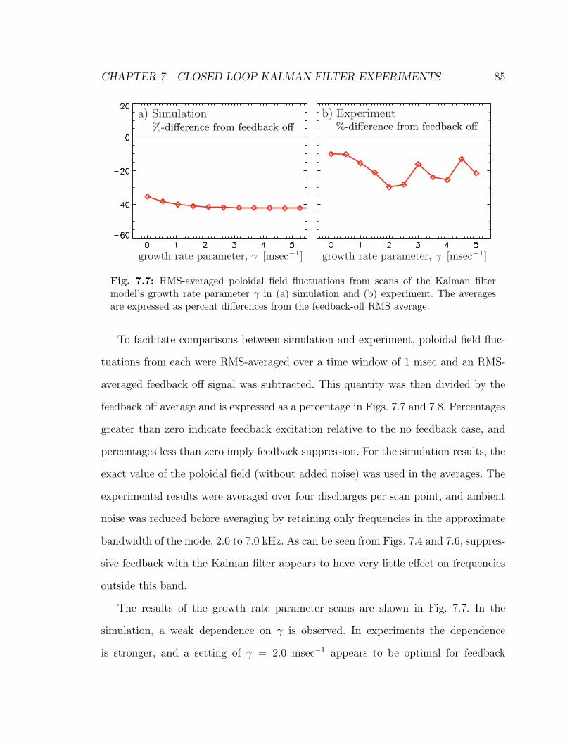
CHAPTER 7. CLOSED LOOP KALMAN FILTER EXPERIMENTS 85
Fig. 7.7: RMS-averaged poloidal field fluctuations from scans of the Kalman filtermodel’s growth rate parameter 𝛾 in (a) simulation and (b) experiment. The averagesare expressed as percent differences from the feedback-off RMS average.
To facilitate comparisons between simulation and experiment, poloidal field fluc-
tuations from each were RMS-averaged over a time window of 1 msec and an RMS-
averaged feedback off signal was subtracted. This quantity was then divided by the
feedback off average and is expressed as a percentage in Figs. 7.7 and 7.8. Percentages
greater than zero indicate feedback excitation relative to the no feedback case, and
percentages less than zero imply feedback suppression. For the simulation results, the
exact value of the poloidal field (without added noise) was used in the averages. The
experimental results were averaged over four discharges per scan point, and ambient
noise was reduced before averaging by retaining only frequencies in the approximate
bandwidth of the mode, 2.0 to 7.0 kHz. As can be seen from Figs. 7.4 and 7.6, suppres-
sive feedback with the Kalman filter appears to have very little effect on frequencies
outside this band.
The results of the growth rate parameter scans are shown in Fig. 7.7. In the
simulation, a weak dependence on 𝛾 is observed. In experiments the dependence
is stronger, and a setting of 𝛾 = 2.0 msec−1 appears to be optimal for feedback

CHAPTER 7. CLOSED LOOP KALMAN FILTER EXPERIMENTS 86
Fig. 7.8: RMS-averaged poloidal field fluctuations from scans of the Kalman filtermodel’s rotation rate parameter 𝜔 in (a) simulation and (b) experiment. The averagesare expressed as percent differences from the feedback-off RMS average. The scans wereperformed at two settings for the diagonal terms in the Kalman filter’s plant noisecovariance matrix, 𝑄𝑖𝑖 = 1× 10⁻⁵ (diamonds), and 𝑄𝑖𝑖 = 1× 10⁻⁴ (stars).
suppression.
Fig. 7.8 shows the results of scans of the Kalman filter’s rotation rate parameter,
𝜔, for settings of the diagonal terms in the plant noise covariance matrix of 𝑄𝑖𝑖 =
1.0×10⁻⁵ and 𝑄𝑖𝑖 = 1.0×10⁻⁴. In both simulation and experiment, feedback is most
effective when the rotation rate parameter is set near that of the natural rotation
frequency of the 𝑛 = 1 mode, about 4 msec−1. Feedback performance decreases as 𝜔
is adjusted in either direction from the optimal value, but the scans performed at the
larger value of 𝑄𝑖𝑖 exhibit less sensitivity to this setting. This result is consistent with
the interpretation of 𝑄 as the amount of uncertainty in the Kalman filter’s internal
model.
While good agreement between simulations made with the reduced Fitzpatrick–
Aydemir model and experimental results is observed, there are several important dif-
ferences between the simulation and experiments. In the reduced Fitzpatrick–Aydemir
model, which is linear, external kink instabilities grow infinitely large in the absence
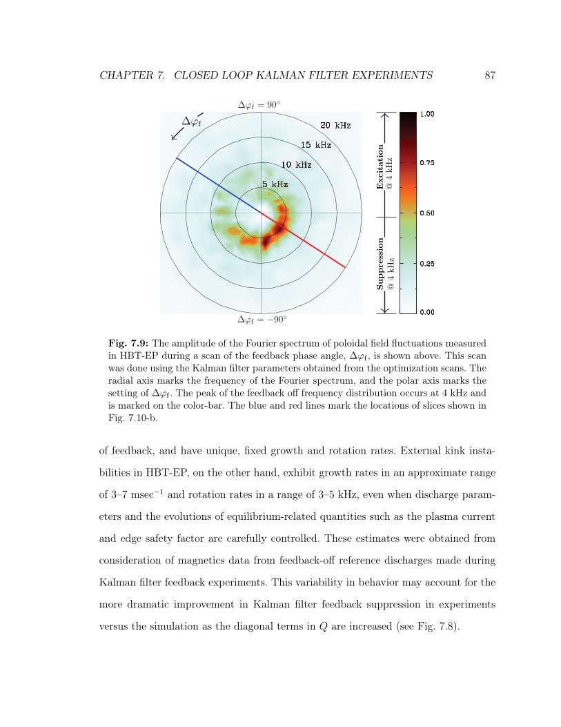
CHAPTER 7. CLOSED LOOP KALMAN FILTER EXPERIMENTS 87
Fig. 7.9: The amplitude of the Fourier spectrum of poloidal field fluctuations measuredin HBT-EP during a scan of the feedback phase angle, Δ𝜙f , is shown above. This scanwas done using the Kalman filter parameters obtained from the optimization scans. Theradial axis marks the frequency of the Fourier spectrum, and the polar axis marks thesetting of Δ𝜙f . The peak of the feedback off frequency distribution occurs at 4 kHz andis marked on the color-bar. The blue and red lines mark the locations of slices shown inFig. 7.10-b.
of feedback, and have unique, fixed growth and rotation rates. External kink insta-
bilities in HBT-EP, on the other hand, exhibit growth rates in an approximate range
of 3–7 msec−1 and rotation rates in a range of 3–5 kHz, even when discharge param-
eters and the evolutions of equilibrium-related quantities such as the plasma current
and edge safety factor are carefully controlled. These estimates were obtained from
consideration of magnetics data from feedback-off reference discharges made during
Kalman filter feedback experiments. This variability in behavior may account for the
more dramatic improvement in Kalman filter feedback suppression in experiments
versus the simulation as the diagonal terms in 𝑄 are increased (see Fig. 7.8).

CHAPTER 7. CLOSED LOOP KALMAN FILTER EXPERIMENTS 88
Fig. 7.10: Fourier spectrum amplitude of poloidal field fluctuations for cases of feedbackexcitation (red, dashed), no feedback (black, solid), and feedback suppression (blue, dot-ted) from experiments (a) before and (b) after optimization of Kalman filter parameters.
7.5 Phase scan with optimized Kalman filter
An optimized Kalman filter was constructed based on the results of the parameter
scans described above, with 𝛾 = 2.0 msec−1, 𝜔 = 2𝜋×4.0 msec−1, and𝑄𝑖𝑖 = 1.0×10⁻⁴.
Fig. 7.9 shows the Fourier spectrum amplitude of poloidal field fluctuations observed
in an experiment with the optimal Kalman filter settings in which the feedback phase
angle is scanned. The results may be directly compared to those from the original
parameter settings, shown in Fig. 7.4. As with the previous results, distinct regions
of feedback suppression and excitation are observed for settings of the feedback phase
angle separated by 180∘.
Performance differences between the original and optimized filters become more
obvious when slices of the contour plots made in the regions of clearest feedback
excitation and suppression are compared with the feedback-off average (see Fig. 7.10).
Choosing more optimal parameters results in enhanced feedback suppression and
excitation.
Further insight into the results of the phase angle scan with the optimized Kalman
filter was obtained using the biorthogonal decomposition (BD) technique described
in Chapter 6. To analyze the phase scan results, (𝑚,𝑛) = (3, 1) and (𝑚,𝑛) = (6, 2)
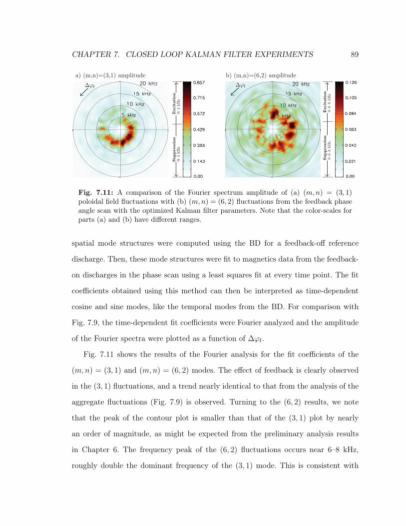
CHAPTER 7. CLOSED LOOP KALMAN FILTER EXPERIMENTS 89
Fig. 7.11: A comparison of the Fourier spectrum amplitude of (a) (𝑚,𝑛) = (3, 1)poloidal field fluctuations with (b) (𝑚,𝑛) = (6, 2) fluctuations from the feedback phaseangle scan with the optimized Kalman filter parameters. Note that the color-scales forparts (a) and (b) have different ranges.
spatial mode structures were computed using the BD for a feedback-off reference
discharge. Then, these mode structures were fit to magnetics data from the feedback-
on discharges in the phase scan using a least squares fit at every time point. The fit
coefficients obtained using this method can then be interpreted as time-dependent
cosine and sine modes, like the temporal modes from the BD. For comparison with
Fig. 7.9, the time-dependent fit coefficients were Fourier analyzed and the amplitude
of the Fourier spectra were plotted as a function of ∆𝜙f .
Fig. 7.11 shows the results of the Fourier analysis for the fit coefficients of the
(𝑚,𝑛) = (3, 1) and (𝑚,𝑛) = (6, 2) modes. The effect of feedback is clearly observed
in the (3, 1) fluctuations, and a trend nearly identical to that from the analysis of the
aggregate fluctuations (Fig. 7.9) is observed. Turning to the (6, 2) results, we note
that the peak of the contour plot is smaller than that of the (3, 1) plot by nearly
an order of magnitude, as might be expected from the preliminary analysis results
in Chapter 6. The frequency peak of the (6, 2) fluctuations occurs near 6–8 kHz,
roughly double the dominant frequency of the (3, 1) mode. This is consistent with

CHAPTER 7 REFERENCES 90
the two modes rotating together rigidly. From the point of view of a sensor coil at a
fixed location, oscillations from the higher spatial harmonic are observed at twice the
frequency of those from the lower harmonic because structure of the higher harmonic
has twice the number of maxima and minima. The effect of feedback on the (6, 2)
mode appears to be weaker than on the (3, 1). However, any activity with 𝑛 = 1 is
explicitly eliminated from feedback signals by the algorithm (see Section 5.3), so it is
expected that feedback will have a negligible effect on the (6, 2) mode.
Chapter 7 references1. G. Bateman, MHD Instablilities, The MIT Press, Cambridge, MA, 1978.
2. A. J. Klein, High-speed digital mode control feedback on Magneto-hydrodynamicinstabilities in the HBT-EP tokamak, PhD thesis, Columbia University, 2005.
3. A. J. Klein, D. A. Maurer, T. Sunn Pedersen, M. E. Mauel, G. A. Navratil,C. Cates, M. Shilov, Y. Liu, N. Stillits, and J. Bialek, Physics of Plasmas 12,040703 (2005).

Chapter 8
Conclusions and future work
The results of simulations and experiments presented in this Thesis show that using
a Kalman filter can improve feedback control of ideal external kink instabilities in the
presence of noise. Remaining questions about optimal feedback algorithm design, kink
mode rigidity, and the impact of control coil size and area coverage will be answered
in future experiments with HBT-EP.
8.1 Conclusions
Simulations and experiments have been used to design, test, and optimize a Kalman
filter for magnetic feedback control of the ideal external kink instability. Successful
control of this instability will improve the energy output and economic viability of
a tokamak fusion reactor. Magnetic feedback systems currently encounter difficulties
with noise in sensor coil measurements, but an optimal filtering method called the
Kalman filter can remove noise from signals. The Kalman filter compares the results
of an internal model for the dynamics of a system with measurements of the system’s
state, producing a realtime estimate of the state that is optimal if the measurements
91

CHAPTER 8. CONCLUSIONS AND FUTURE WORK 92
are tainted by Gaussian noise. For the work presented here, the Kalman filter’s internal
model is derived from the insight that the external kink mode exhibits two basic
behaviors: rigid rotation and exponential growth.
The reduced Fitzpatrick–Aydemir model was used to simulate external kink mode
feedback in HBT-EP. The model is a straightforward set of ordinary differential equa-
tions, but it captures the physics required to simulate external kink mode feedback in
the high plasma dissipation limit. The effects of the plasma equilibrium, plasma rota-
tion, plasma energy dissipation, plasma–wall coupling, and plasma–feedback coupling
impact the stability of the external kink mode and are included in the simulation.
In simulations with the reduced Fitzpatrick–Aydemir equations, the Kalman filter
removed added noise from the measurements used to compute the feedback signal.
In time-dependent simulation runs, using the Kalman filter brought about a 50%
reduction in peak control power compared with results from the case of noisy mea-
surements with no Kalman filter. In addition, a 92% reduction in mean control power
was achieved in the time interval after the mode had been stabilized by feedback.
The Kalman filter algorithm was implemented on a set of low-latency field pro-
grammable gate array controllers for feedback studies on the HBT-EP experiment.
The controllers are coupled to the plasma via an array of 20 poloidal field sensors and
a corresponding array of 20 pairs of radial control coils. The control coils are small
and localized, covering about 15% of the plasma surface.
External kink unstable plasma discharges were prepared in HBT-EP for experi-
mental testing of the Kalman filter algorithm. In these discharges, external kink modes
were observed to last for about 1 msec. A dominant (𝑚,𝑛) = (3, 1) structure, resonant
with the value of the safety factor just outside the plasma edge, was observed. The
modes had an average growth rate of 5 msec−1, and rotation rates ranging between
3–5 kHz.
CHAPTER 8. CONCLUSIONS AND FUTURE WORK 93
In experimental scans of the spatial phasing between the instability and feedback,
the Kalman filter algorithm suppressed the mode over a broad range of phase angles.
In contrast to the results of prior experiments performed without the Kalman filter,
excitation of frequencies above the natural rotation frequency of the external kink
mode was minimal at all phasings.
Additional noise with a white frequency spectrum and Gaussian probability dis-
tribution was added to measurements inside the feedback algorithm for feedback sup-
pression and excitation experiments with and without the Kalman filter. The Kalman
filter was found to remove much of this noise from output signals. In these experi-
ments, the algorithm with the Kalman filter retained its ability to suppress and excite
the external kink under noise levels that impaired feedback without the Kalman filter.
Scans of the Kalman filter’s growth and rotation rate parameters were performed
in both simulations and experiments to determine their optimal values. The simulation
results were in qualitative agreement with those from the experiments. Scans of the
rotation rate parameter were performed at two values of the uncertainty parameter for
the Kalman filter’s internal model, with the finding that increasing this uncertainty
improved feedback suppression and weakened the dependence on the rotation rate
parameter. The results of the scans were used to construct an optimized Kalman
filter that was tested in a feedback phase angle scan. A comparison of the feedback
phase angle scan results for the original and optimized Kalman filters led to the
conclusion that the optimized parameter values improved both feedback suppression
and excitation.
Further analysis of the phase scan results showed some evidence of magnetic activ-
ity with an (𝑚,𝑛) = (6, 2) harmonic and coexisting with the dominant (𝑚,𝑛) = (3, 1)
activity. The (6, 2) mode had about twice the rotational frequency of the (3, 1) mode.
The (6, 2) mode was found to be largely unaffected by feedback, probably because the
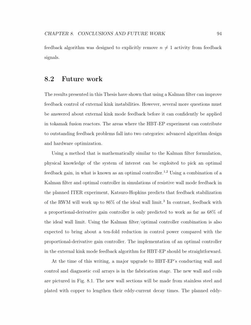
CHAPTER 8. CONCLUSIONS AND FUTURE WORK 94
feedback algorithm was designed to explicitly remove 𝑛 = 1 activity from feedback
signals.
8.2 Future work
The results presented in this Thesis have shown that using a Kalman filter can improve
feedback control of external kink instabilities. However, several more questions must
be answered about external kink mode feedback before it can confidently be applied
in tokamak fusion reactors. The areas where the HBT-EP experiment can contribute
to outstanding feedback problems fall into two categories: advanced algorithm design
and hardware optimization.
Using a method that is mathematically similar to the Kalman filter formulation,
physical knowledge of the system of interest can be exploited to pick an optimal
feedback gain, in what is known as an optimal controller.1,2 Using a combination of a
Kalman filter and optimal controller in simulations of resistive wall mode feedback in
the planned ITER experiment, Katsuro-Hopkins predicts that feedback stabilization
of the RWM will work up to 86% of the ideal wall limit.3 In contrast, feedback with
a proportional-derivative gain controller is only predicted to work as far as 68% of
the ideal wall limit. Using the Kalman filter/optimal controller combination is also
expected to bring about a ten-fold reduction in control power compared with the
proportional-derivative gain controller. The implementation of an optimal controller
in the external kink mode feedback algorithm for HBT-EP should be straightforward.
At the time of this writing, a major upgrade to HBT-EP’s conducting wall and
control and diagnostic coil arrays is in the fabrication stage. The new wall and coils
are pictured in Fig. 8.1. The new wall sections will be made from stainless steel and
plated with copper to lengthen their eddy-current decay times. The planned eddy-

CHAPTER 8. CONCLUSIONS AND FUTURE WORK 95
Fig. 8.1: Diagram of the planned first wall and feedback system upgrade for HBT-EP.
current decay timescale will be close to that of the hybrid stainless steel and aluminum
wall presently in place.
A total of 40 poloidal field coils will enhance the sensory ability of the feedback
system and lead to improved understanding of the spatial structure of instabilities.
Previous experiments4 have indicated that the external kink mode can respond non-
rigidly to feedback. The increased diagnostic coverage installed as part of the wall
upgrade will help quantify this behavior.
The impact of control coil coverage and modularity will be addressed by exper-
iments with 60 new control coils at 10 toroidal locations. Small, modular, internal
MHD control coils similar to these are now planned for the ITER experiment.5 The
new control coil set planned for HBT-EP will answer questions about whether the
response of the external kink mode to feedback is rigid under changes in the area
coverage of the control coils and changes in control coil size. A numerical analysis
of the vacuum spectra of these coils performed by Klein6 showed that the relative

CHAPTER 8 REFERENCES 96
magnitude of sideband harmonics unrelated to the specified control field increases as
progressively smaller coils are used.
Chapter 8 references1. R. E. Kalman, Transactions of the ASME–Journal of Basic Engineering 82, 35
(1960).
2. B. Friedland, Control System Design: An Introduction to State-Space Methods,McGraw-Hill, New York, 1986.
3. O. Katsuro-Hopkins, J. Bialek, D. Maurer, and G. Navratil, Nuclear Fusion 47,1157 (2007).
4. T. Sunn Pedersen, D. A. Maurer, J. Bialek, O. Katsuro-Hopkins, J. M. Hanson,M. E. Mauel, R. James, A. Klein, Y. Liu, and G. A. Navratil, Nuclear Fusion47, 1293 (2007).
5. R. J. Hawryluk, Principle physics developments evaluated in the iter designreview, in Proc. 22nd Int. Conf. on Fusion Energy (Geneva, Switzerland), pageIT/102, Vienna, IAEA, 2008.
6. A. J. Klein, High-speed digital mode control feedback on Magneto-hydrodynamicinstabilities in the HBT-EP tokamak, PhD thesis, Columbia University, 2005.

Appendix A
FPGA programming considerations
Circuit design for the NI 7831-R FPGA controllers is done using a special subset
of the National Instruments LabVIEW programming language that is restricted to
integer operations. Mathematical precision is retained by casting the 16-bit integers
obtained from the FPGAs’ analog-to-digital convertors as 32-bit and by rescaling
during numerical operations by powers of 2 to make good use of the 32-bit range.
Small constants, such as the DFT coefficients, are scaled up before they are used
in the algorithm. For example, the operation 𝑦 = 0.5𝑥 might be implemented as
𝑦 = (512𝑥)× 2−10.
An automatic compile process maps a program written in LabVIEW to relatively
low-level Hardware Description Language (HDL) code, and subsequently maps the
HDL to a design for the actual FPGA. The compile process is iterative and the user
has some control over how the design is optimized. For example, the compiler can be
instructed to optimize a design either to conserve physical resources on the FPGA or
to minimize execution time. Another parameter dictates the amount of “effort” the
compiler puts into the optimization; increasing the effort can significantly increase the
compile time. In order to reduce loop latency, a speed optimization with relatively97

APPENDIX A. FPGA PROGRAMMING CONSIDERATIONS 98
high effort was chosen for the algorithm described in Chapter 5. Estimates of the
latency were obtained by sending a known input into the FPGA at a specified time
and measuring the time required for the FPGA to produce the expected output.
Additional reductions in latency were achieved by making adjustments to the
LabVIEW code for the control algorithm and compiling and measuring the latency of
the design after every adjustment. Subroutines in the LabVIEW code can be either
specified as “reentrant,” meaning that a physical copy of the subroutine is made on
the FPGA for each instance where it is required by the algorithm, or “non-reentrant,”
meaning that only a single copy of the subroutine is made, and calls to this sub-
routine from the algorithm must be arbitrated. Furthermore, different portions of an
algorithm can be specified to execute either in series or in parallel. When minimizing
algorithm latency is a priority, it is best to use reentrant subroutines and execute
pieces of large algorithms in parallel. However, the extent to which reentrant subrou-
tines can be used is limited by the size of the subroutines and the number of copies
required due to the finite number of components in the FPGA. The compiler pro-
vides a detailed report on the FPGA resource usage for a particular design. These
and additional optimization techniques are discussed in greater detail in Ref. 1.
To optimize the algorithm described here, the algorithm was first broken into small
stages that were compiled and benchmarked individually. Stages that had larger la-
tencies were then designated to execute in parallel with one another, and reentrant
subroutines were employed when possible to maximize usage of the FPGA’s compo-
nents. An iterative application of these techniques was used to obtain a latency of 12
𝜇sec for the feedback algorithm, a five-fold reduction compared with the original.
Further documentation and optimization advice are available on the National
Instruments website.2
APPENDIX A REFERENCES 99
Appendix A references1. J. DiGiovanni, Advanced LabVIEW FPGA Programming: Optimizing for Speed
and Size, URL ftp://ftp.ni.com/pub/devzone/advancedfpgaprogramming.ppt,2005.
2. National Instruments, URL http://www.ni.com/.

Appendix B
Feedback algorithm
This Appendix provides a more exact discussion of the feedback algorithm outlined in
Chapter 5. A detailed explanation of all the steps in the feedback algorithm is given,
followed by a step-by-step description of how the algorithm is implemented.
The FPGA controllers do not support floating-point operations, so all the cal-
culations described below are done using integers. To retain precision in multiply
operations involving coefficients with magnitudes of order unity or smaller, the coef-
ficients are scaled up by a power of 2 before being stored in memory on the FPGA
controllers. The result of the multiply operation is then divided by the same power
of 2.
B.1 Equations solved
The first step in the algorithm is a spatial filter that selects the 𝑛 = 1 component of
a five-element vector of sensor coil inputs using a discrete Fourier transform (DFT)
100

APPENDIX B. FEEDBACK ALGORITHM 101
matrix multiply. The 𝑛 = 1 cosine and sine modes, 𝑦cos and 𝑦sin, are given by
⎛⎜⎝𝑦cos
𝑦sin
⎞⎟⎠ = 𝐷× 2−10, (B.1)
where the matrix 𝐷 is a 2× 5 matrix containing the 𝑛 = 1 rows of a DFT times the
Kalman gain and a factor of 220,
𝐷 =2
5
⎛⎜⎝cos 0 cos 2𝜋/5 cos 4𝜋/5 cos 6𝜋/5 cos 8𝜋/5
sin 0 sin 2𝜋/5 sin 4𝜋/5 sin 6𝜋/5 sin 8𝜋/5
⎞⎟⎠𝐾 × 220.
The Kalman gain, 𝐾 = 0.01614, is “pre-multiplied” with the DFT matrix in order
to save multiply operations on the FPGAs. Generally, 𝐾 is a matrix (see Eq. 4.20),
but, for the case of the matrices chosen to describe the external kink mode feedback
problem (see Section 4.4), 𝐾 can be written as a scalar times the identity matrix.
Note that Eq. B.1 contains a scale factor of 2−10 while the matrix 𝐷 is scaled up
by 220. The remaining factor of 210 is propagated through until Eq. B.3, to retain
precision in that calculation.
A first order, phase-lag temporal filter follows the spatial filter. The first order
temporal filter is a recursive equation in which the filter’s output 𝑧𝑖 at time step 𝑖
depends on an input 𝑦𝑖, as well as the previous output and input, 𝑧𝑖−1 and 𝑦𝑖−1. It is no-
tationally more convenient to keep track of these terms in a vector 𝑝 = [𝑦𝑖, 𝑦𝑖−1, 𝑧𝑖−1].
The first term in 𝑝, the filter’s input, is set equal to one of 𝑦cos or 𝑦sin. The filter’s
output is then given by
𝑧𝑖 =∑
0≤𝑘<3
𝑝[𝑘]𝑎lag[𝑘]. (B.2)
Some reassignment of the terms in 𝑝 is then required for the next time step, namely,

APPENDIX B. FEEDBACK ALGORITHM 102
𝑝[1] = 𝑝[0]𝑎lag [0] × 2−10, and 𝑝[2] = 𝑧𝑖 × 2−10. In this notation, square brackets are
used to subscript a vector starting from index 0, that is, 𝑝[0] denotes the first element
of 𝑝. The vector of filter coefficients is given by lag = [1.0743,−0.83008, 0.9922]×210.
The components of lag were calculated by manually adjusting their effect on the
combined transfer function of the hardware elements preceding the FPGA controllers
in the feedback loop.
The form of the phase-lead temporal filter is identical to Eq. B.2, except for the fact
that a different vector of coefficients is used: lead = [2.051,−0.889,−0.0977] × 210.
These coefficients are chosen to compensate for the transfer function of hardware
components following the FPGA controllers in the feedback loop.
The Kalman filter’s estimate ˆ𝑥 for the current time step is given by the recursive
equation
ˆ𝑥𝑖 = (Φˆ𝑥𝑖−1 + 𝑖)× 2−10. (B.3)
The four-element measurement vector is formed using the output of the lag filter
after it has acted on both 𝑦cos and 𝑦sin. The first two elements of correspond to
the cosine and sine modes of the control flux and are always null because this flux is
simulated by the Kalman filter but not measured directly. Usually, Eq. B.3 is written
with a factor of the Kalman gain 𝐾 appearing in front of . In this case, however,
the Kalman gain is pre-multiplied with the 𝐷 matrix (see Eq. B.1). The Φ matrix is
calculated as in Eq. 4.19, using the terms defined in Section 4.4,
Φ =
⎛⎜⎜⎜⎜⎜⎜⎜⎝
0.960693 0 0.017643 0
0 0.960693 0 0.017643
−0.147091 0 0.980510 0.100003
0 −0.147091 −0.100003 0.980510
⎞⎟⎟⎟⎟⎟⎟⎟⎠× 210.

APPENDIX B. FEEDBACK ALGORITHM 103
The final stage of the algorithm involves mapping the filtered cosine and sine
modes back to real space using an inverse DFT. Given the cosine and sine modes,
𝑦cos and 𝑦sin obtained from the forward DFT and filtered by the phase-lag, Kalman,
and phase-lead filters, the five-element vector of outputs for the control coils is given
by
= 𝐷−1
⎛⎜⎝𝑦cos
𝑦sin
⎞⎟⎠ . (B.4)
Here, 𝐷−1 not strictly the inverse of 𝐷 from Eq. B.1. It is a 5×2 matrix consisting of
the 𝑛 = 1 columns of an inverted, 5× 5 DFT matrix, pre-multiplied with a rotation
operator and a proportional gain coefficient 𝐺,
𝐷−1 =
⎛⎜⎜⎜⎜⎜⎜⎜⎜⎜⎜⎝
cos 0 sin 0
cos 2𝜋/5 sin 2𝜋/5
cos 4𝜋/5 sin 4𝜋/5
cos 6𝜋/5 sin 6𝜋/5
cos 8𝜋/5 sin 8𝜋/5
⎞⎟⎟⎟⎟⎟⎟⎟⎟⎟⎟⎠
⎛⎜⎝cos ∆𝜙f − sin ∆𝜙f
sin ∆𝜙f cos ∆𝜙f
⎞⎟⎠𝐺× 210.
The toroidal phase angle ∆𝜙f is chosen at run time. Setting ∆𝜙f has the effect of
shifting the toroidal phase of feedback with respect to that of the instability. The
proportional gain setting 𝐺 = 4 was experimentally determined to be optimal for
feedback suppression of the external kink instability.
B.2 Description of the algorithm
Here is a description of how to perform the feedback algorithm that closely follows the
actual implementation on the NI 7831-R FPGA controllers. Because the controllers
a programmed using a “visual” language called LabVIEW, it is difficult to represent

APPENDIX B. FEEDBACK ALGORITHM 104
Fig. B.1: A flow chart for the Kalman filter algorithm.
the implementation of the algorithm using words. Loosely speaking, programming in
LabVIEW involves drawing a block diagram for the program. However, the diagram-
ming symbols used in LabVIEW are non-standard, and pictures of the LabVIEW
code are difficult for those unacquainted with the language to understand. Thus a
step-by-step description of the algorithm is provided, accompanied by a high-level
flow chart (Fig. B.1).
In the exposition that follows, a left-pointing arrow (←) is used to denote the
assignment of a number to a variable, as in 𝑥 ← 3. Pairs of numbers in brackets are
used to subscript the matrix Φ; for example, Φ[0, 1] indicates the element at the first
row and second column of Φ. Also, the inputs from the sensor coils, , are assumed
to be assigned by the FPGA controller for every iteration, so they are not explicitly
assigned below.
All the variables below are taken to be 32-bit integers. In the event that any of
the calculations overflow the 32-bit range, given by [−231, 231 − 1], the results are
“wrapped around” to the other side of the range. For example, the result of −231 − 1
is 231 − 1.
K0. [Initialize.] Set all the state variables for the phase-lag, phase-lead, and Kalman
filters to zero: for 1 ≤ 𝑘 < 3, set 𝑝coslag [𝑘], 𝑝 sin
lag [𝑘], 𝑝coslead[𝑘], and 𝑝 sin
lead[𝑘] ← 0, and
for 0 ≤ 𝑘 < 4, set 𝑥[𝑘] ← 0. Assign to 𝐷, lag , Φ, lead, and 𝐷−1 the values
given in Section B.1, rounded to the nearest integer.

APPENDIX B. FEEDBACK ALGORITHM 105
K1. [Forward spatial filter.] Set 𝑝coslag [0] ← 0 and 𝑝 sin
lag [0] ← 0. For 0 ≤ 𝑘 < 5 set
𝑝coslag [0]← 𝑝cos
lag [0] + (𝑠[𝑘]𝐷[0, 𝑘])× 2−10, and set 𝑝 sinlag [0]← 𝑝 sin
lag [0] + (𝑠[𝑘]𝐷[1, 𝑘])×
2−10.
K2. [Lag temporal filter.] Do the operations temporalFilter(𝑝 coslag , lag) and
temporalFilter(𝑝 sinlag , lag).
The operation temporalFilter(𝑝, ) is defined as follows for the three-
element vectors 𝑝 and . Set a temporary variable 𝑧 ← 0. For 0 ≤ 𝑘 < 3,
set 𝑧 ← 𝑧 + 𝑝[𝑘]𝑎[𝑘]. Now, reassign and rescale the elements in 𝑝: set 𝑝[1] ←
(𝑝[0]𝑎[0])× 2−10 and 𝑝[2]← 𝑧 × 2−10.
K3. [Kalman filter.] Multiply the Φ matrix by : for 0 ≤ 𝑗 < 4, set 𝑥[𝑗] ←∑0≤𝑘<4 Φ[𝑗, 𝑘]𝑥[𝑘]. Now, mix in the lag-filtered measurements: set 𝑥[2]← (𝑥[2]+
𝑝coslag [2])× 2−10 and 𝑥[3]← (𝑥[3] + 𝑝 sin
lag [2])× 2−10.
K4. [Lead temporal filter.] Set 𝑝coslead[0] ← 𝑥[2] and 𝑝 sin
lead[0] ← 𝑥[3]. Now do the
operations temporalFilter(𝑝 coslead, lead) and temporalFilter(𝑝 sin
lead, lead).
K5. [Reverse spatial filter.] For 0 ≤ 𝑘 < 5, set 𝑐[𝑘] ← (𝐷−1[0, 𝑘] 𝑝coslead[3]) × 2−10 +
(𝐷−1[1, 𝑘] 𝑝 sinlead[3])× 2−10.
K6. [Repeat.] Return to K1.