Comparative Study of Tracking Application Using Extended

Kalman Filter and Unscented Kalman Filter

Kalman Filter is an estimator i.e. used for estimating the instantaneous state of a dynamic system

perturbed by white noise – by using measurements related to the state but corrupted by white noise. The Kalman filter operates on estimating states by using recursive time and measurement updates over time.

The most immediate applications of Kalman Filter are related to Tracking, be it tracking paths of missile

ships & aircrafts or tracking the pattern of images or tracking an object or tracking of maximum power point or tracking the prices of various commodities or tracking of stock market. In other words it is used

to control a dynamic system. For these applications, it is not always possible or desirable to measure

every variable that one wants to control and Kalman filter provides a mean for inferring the missing information from noisy environments.

Some of these systems show linear behavior while others show non linear behavior. Rudolph E. Kalman

introduced his recursive approach to solve a linear filtering problem in 1960. Later this problem has been extended to solving the nonlinear systems which gave rise to Extended Kalman Filter. In the extended

Kalman filter (EKF), the state transition and observation models need not be linear functions of the state

but may instead be non linear functions. However, this non linear version of Kalman filter linearizes about the estimate of current mean and covariance.

When the state transition and observation models are highly non linear, it was observed that extended Kalman filter can give particularly poor performance and then Unscented Kalman Filter came into picture

which uses a deterministic sampling technique known as the unscented transform (given in detail later) to

pick a minimal set of sample points (called sigma points) around the mean.

In this report we lay our focus on comparative study of Extended Kalman filter and Unscented Kalman

filter for one of the most important and extensively used application of tracking i.e. maximum power

point tracking. In further sections we would see the description of maximum power point tracking and the simulations of extended Kalman filter and unscented Kalman filter.

EXTENDED KALMAN FILTER

In Extended Kalman Filter the state process and measurement models need not be linear functions of state

but may instead be differentiable functions. Let the state be given by the following non linear equation

[2]-

𝑥𝑘 = 𝑓(𝑥𝑘−1,𝑢𝑘−1,𝑤𝑘−1), here f(.,.,.) is the process model, xk-1 is the state of the system at time step k-1,

uk-1 is the input vector and wk-1 is the noise.

and the measurement be given by –

𝑧𝑘 = ℎ(𝑥𝑘 , 𝑣𝑘) , here h(.,.) is the observation model that transforms the state vector space into

observation space and vk is the measurement noise.

The random variables wk and vk again represent the process and measurement noise with Q (process noise

covariance) and R (measurement noise covariance).

The function f is used to compute the predicted state from the earlier estimation i.e. relates the state at

previous time step k-1 to the state at the current time step k. It includes driving function uk-1 and the zero

mean process noise wk. The function h is used to compute the predicted measurement from the predicted

state i.e. xk to zk. At each time step the Jacobian is evaluated. These matrices are used in the Kalman Filter

equations [2].

𝑥 𝑘 is a posteriori estimate and 𝑥 𝑘−is a priori estimate.

The state transition matrices and observation matrices are defined by the following Jacobians –

𝐴𝑘 = 𝜕𝑓

𝜕𝑥(𝑥 𝑘 ,𝑢𝑘)

𝐵𝑘 = 𝜕ℎ

𝜕𝑥(𝑥 𝑘

−)

The given equations represent the time update and measurement updates for an extended Kalman filter

(EKF).

Time Update (“Prediction”)

𝑥 𝑘− = 𝑓 𝑥 𝑘−1,𝑢𝑘−1 (Prediction State Estimate)

𝑃𝑘− = 𝐴𝑘𝑃𝑘−1𝐴𝑘

𝑇 + 𝑄𝑘−1 (Prediction Covariance Estimate)

Measurement Update (“Correction”)

𝐾𝑘 = 𝑃𝑘−𝐵𝑘

𝑇( 𝐵𝑘𝑃𝑘−𝐵𝑘

𝑇 + 𝑅𝑘)−1 (Kalman Gain)

𝑥 𝑘 = 𝑥 𝑘− + 𝐾𝑘 (𝑧𝑘 − ℎ 𝑥 𝑘

− ) (Updated State Estimate)

𝑃𝑘 = (𝐼 − 𝐾𝑘𝐵𝑘)𝑃𝑘− (Updated Estimate Covariance)

An important feature of the EKF is that the Jacobian 𝐵𝑘 in the equation for the Kalman gain 𝐾𝑘 serves to correctly propagate or “magnify” only the relevant component of the measurement information. For

example, if there is no one-to-one mapping between the measurement 𝑧𝑘 and the state via h, 𝐵𝑘 affects

the Kalman gain and it magnifies the portion of the residual 𝑧𝑘 − ℎ 𝑥 𝑘− which affects the state. If, for all

measurements there is no one-to-one mapping between the measurement 𝑧𝑘 and the state via h, then he

filter will quickly diverge hence making the process unobservable [2].

UNSCENTED KALMAN FILTER For much complex non linear systems i.e. higher order calculations we use another version i.e. Unscented

Kalman Filter (UKF). The Unscented Kalman Filter was 1st proposed by Jeffery Uhlman [4].

The state distribution is specified by a minimal set of carefully chosen sample points. These sample points

capture the mean and covariance of the random variable and when propagated through a non linear

system, captures the mean and covariance.

Unscented Transformation:-

The unscented transformation (UT) is a method for calculating the statistics of a random variable which

undergoes a nonlinear transformation. Consider propagating a random variable x (dimension L) through a

nonlinear function, y = f(x). Assume, x has mean and covariance Px. To calculate the statistics of y, we

form a matrix X of 2L+1 sigma vectors Xi as given by the equations [1] mentioned below:

,

, i = 1,…,L

, i=L+1,…,2L

is a scaling parameter. The constant determines the spread of the sigma points

around and is usually a small positive value (1 < < 1e-4). The constant is secondary scaling

parameter which is usually set to 0 or 3-L. is the ith

column of the matrix square root.

The sigma vectors are propagated through a non linear function Yi = f(Xi) where i = 0,…,2L, while the

mean and covariance for y are approximated using a weighted sample mean and covariance of the sigma

points.

β incorporates the prior knowledge of the distribution of x.

is the process noise covariance and is the measurement noise covariance. Weights are already

calculated according to the equations presented earlier.

In case of additive noise the initialization remains same but the noise is directly added in case of time

update and measurement update equations.

Initialization:

Sigma points:

Time Update:

Here we need to redraw a new set of sigma points to incorporate the effect of additive process noise.

Measurement Update:

The above cycle continues till the sigma points come really closer.

Maximum Power Point Tracking (MPPT)

Solar cells have a complex relationship between solar irradiation, temperature and total resistance that produces a non linear output efficiency which can be analyzed based on the I-V curve. The power P is

given by P=V*I. A photovoltaic cell, for the majority of its useful curve, acts as a constant current source.

However, at a photovoltaic cell's MPP region, its curve has an approximately inverse exponential relationship between current and voltage. From basic circuit theory, the power delivered from or to a

device is optimized where the derivative (graphically, the slope) dI/dV of the I-V curve is equal and

opposite the I/V ratio (where dP/dV=0). Hence, a solar photovoltaic array should work at maximum power point to deliver maximum operational efficiency.

MPPT is a technique that inverters, battery chargers and other similar devices use to get maximum

possible power from photovoltaic devices. This is known as the maximum power point (MPP) and corresponds to the knee of the curve [3]. A load with resistance R=V/I equal to the reciprocal of this value

draws the maximum power from the device. This is sometimes called the characteristic resistance of the

cell. This is a dynamic quantity which changes depending on the level of illumination, as well as other factors such as temperature and the age of the cell. If the resistance is lower or higher than this value, the

power drawn will be less than the maximum available, and thus the cell will not be used as efficiently as

it could be.

Maximum power point trackers utilize different types of control circuit or logic to search for this point

and thus to allow the converter circuit to extract the maximum power available from a cell. For any given

set of operational conditions, cells have a single operating point where the values of the current (I) and Voltage (V) of the cell result in a maximum power output. These values correspond to a particular load

resistance, which is equal to V / I as specified by Ohm's Law.

CHARACTERISTICS OF PV ARRAY

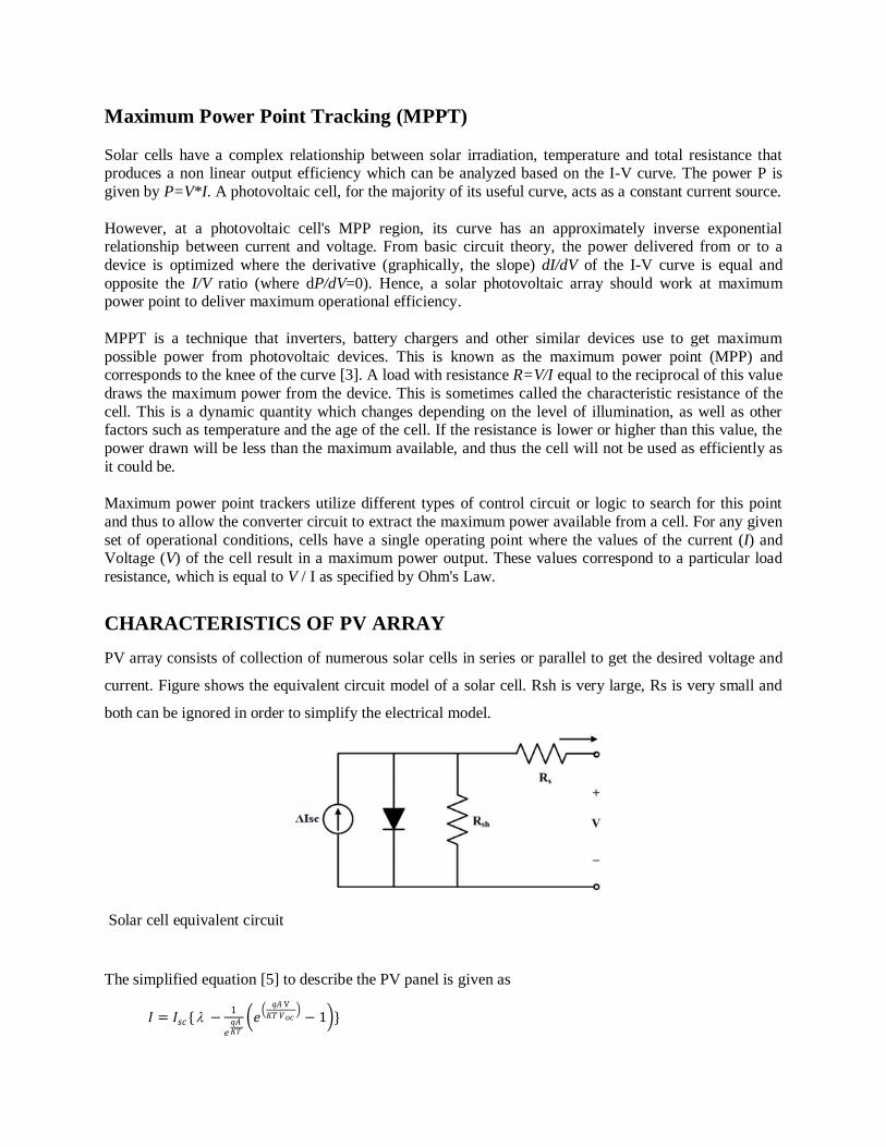
PV array consists of collection of numerous solar cells in series or parallel to get the desired voltage and

current. Figure shows the equivalent circuit model of a solar cell. Rsh is very large, Rs is very small and

both can be ignored in order to simplify the electrical model.

Solar cell equivalent circuit

The simplified equation [5] to describe the PV panel is given as

𝐼 = 𝐼𝑠𝑐 { −1

𝑒𝑞𝐴𝐾𝑇

𝑒

𝑞𝐴 V

𝐾𝑇 𝑉𝑜𝑐 − 1 }

where Voc and Isc are open circuit voltage and current values at 1kW/m2 and 25

0C. T is the temperature of

array in 0

C, q is the elementary charge, k is the Boltzmann constant, is irradiance in kW/m2andA is a

constant, generally taken as 0.2464. V and I are the array output voltage and current.

MPPT USING EXTENDED KALMAN FILTER APPROACH

The PV relation for a solar array is a non linear one. In this section MPPT using extended Kalman filter is

proposed. A Kalman Filter that becomes linear about estimates of current mean and covariance is referred

to as Extended Kalman filter.

𝑑P

𝑑V=𝑑(VI)

𝑑(V)= I + V

𝑑I

𝑑V

V𝑑I

𝑑V=−VIsc

𝑒𝑞𝐴𝐾𝑇

{𝑞𝐴

𝐾𝑇𝑉𝑜𝑐𝑒

𝑞𝐴V𝐾𝑇𝑉𝑜𝑐 }

According to the P – V curve power increases with a gradual positive slope until reaches one optimal

point and decreases after that steeply. MPPT algorithm is governed by the given state equation where

Vactualt+1 is the value of voltage updated by the MPPT controller at iteration t+1,

𝑑P

𝑑V is the slope of the P-V

curve and w be the additive noise.

Vactualt+1 = Vactual

t + 𝑀𝑑P

𝑑V+ 𝑤

Vref t − Vactual

t = h

V t− = V t−1 + 𝑀𝐼sc −

1

𝑒𝑞𝐴𝐾𝑇

𝑞𝐴

𝐾𝑇𝑉𝑜𝑐𝑒 𝑞𝐴 V t−1𝐾𝑇 𝑉𝑜𝑐

+ 𝑒

𝑞𝐴 V t−1𝐾𝑇 𝑉𝑜𝑐

− 1 , where V t

−is the predicted

estimate of voltage at step t while V t−1 is the corrected estimate for the step t-1.

𝐴𝑘 = 1

𝑑(V t + 𝑀𝐼sc −1

𝑒𝑞𝐴𝐾𝑇

𝑞𝐴

𝐾𝑇𝑉𝑜𝑐𝑒 𝑞𝐴V t𝐾𝑇𝑉𝑜𝑐

+ 𝑒

𝑞𝐴V t𝐾𝑇𝑉𝑜𝑐

− 1 )

𝑑V t

𝐵𝑘= 1 +

𝑑(V t +𝑀𝐼sc −1

𝑒𝑞𝐴𝐾𝑇

𝑞𝐴

𝐾𝑇𝑉𝑜𝑐𝑒 𝑞𝐴 V t𝐾𝑇𝑉𝑜𝑐

+𝑒

𝑞𝐴V t𝐾𝑇𝑉𝑜𝑐

−1 )

𝑑V t

Initially we start with 𝑃𝑘 = 0.1 and will continue to run the simulations till Pk approaches zero meaning

the noise has been reduced to a great extent.

MPPT USING UNSCENTED KALMAN FILTER APPROACH

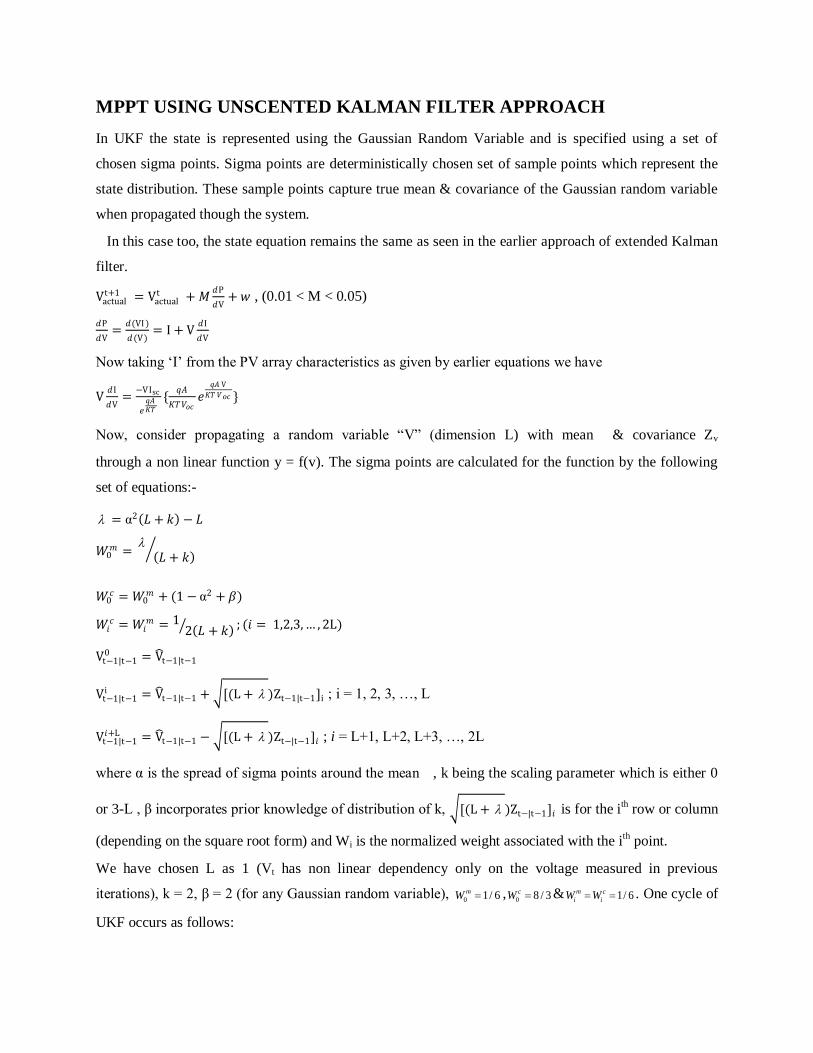
In UKF the state is represented using the Gaussian Random Variable and is specified using a set of

chosen sigma points. Sigma points are deterministically chosen set of sample points which represent the

state distribution. These sample points capture true mean & covariance of the Gaussian random variable

when propagated though the system.

In this case too, the state equation remains the same as seen in the earlier approach of extended Kalman

filter.

Vactualt+1 = Vactual

t + 𝑀𝑑P

𝑑V+ 𝑤 , (0.01 < M < 0.05)

𝑑P

𝑑V=

𝑑(VI )

𝑑(V)= I + V

𝑑I

𝑑V

Now taking „I‟ from the PV array characteristics as given by earlier equations we have

V𝑑I

𝑑V=

−VIsc

𝑒𝑞𝐴𝐾𝑇

{𝑞𝐴

𝐾𝑇𝑉𝑜𝑐𝑒

𝑞𝐴 V

𝐾𝑇 𝑉𝑜𝑐 }

Now, consider propagating a random variable “V” (dimension L) with mean & covariance Zv

through a non linear function y = f(v). The sigma points are calculated for the function by the following

set of equations:-

= α2 𝐿 + 𝑘 − 𝐿

𝑊0𝑚 =

𝐿 + 𝑘

𝑊0𝑐 = 𝑊0

𝑚 + (1 − α2 + 𝛽)

𝑊𝑖𝑐 = 𝑊𝑖

𝑚 = 12 𝐿 + 𝑘 ; (𝑖 = 1,2,3,… , 2L)

Vt−1|t−10 = V t−1|t−1

Vt−1|t−1i = V t−1|t−1 + [(L + )Zt−1|t−1]i ; i = 1, 2, 3, …, L

Vt−1|t−1𝑖+L = V t−1|t−1 − [(L + )Zt−|t−1]𝑖 ; i = L+1, L+2, L+3, …, 2L

where α is the spread of sigma points around the mean , k being the scaling parameter which is either 0

or 3-L , β incorporates prior knowledge of distribution of k, [(L + )Zt−|t−1]𝑖 is for the ith row or column

(depending on the square root form) and Wi is the normalized weight associated with the ith point.

We have chosen L as 1 (Vt has non linear dependency only on the voltage measured in previous

iterations), k = 2, β = 2 (for any Gaussian random variable), 0 1/ 6mW ,

0 8 / 3cW & 1/ 6m c

i iW W . One cycle of

UKF occurs as follows:

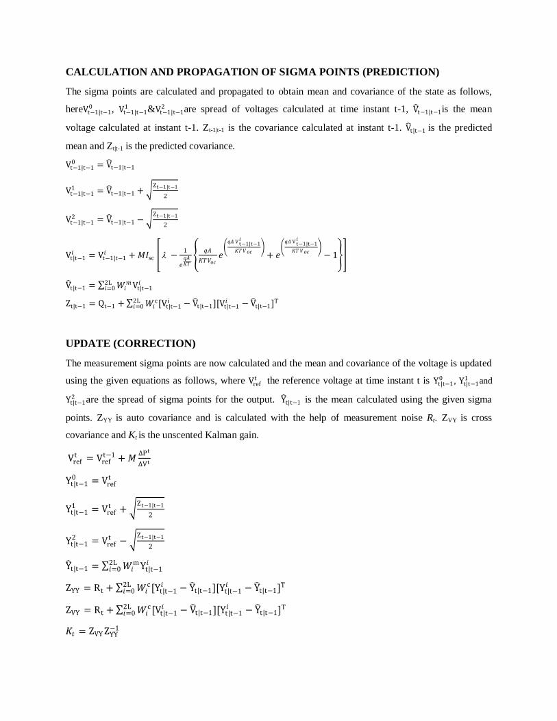
CALCULATION AND PROPAGATION OF SIGMA POINTS (PREDICTION)

The sigma points are calculated and propagated to obtain mean and covariance of the state as follows,

hereVt−1|t−10 , Vt−1|t−1

1 &Vt−1|t−12 are spread of voltages calculated at time instant t-1, V t−1|t−1is the mean

voltage calculated at instant t-1. Zt-1|t-1 is the covariance calculated at instant t-1. V t|t−1 is the predicted

mean and Zt|t-1 is the predicted covariance.

Vt−1|t−10 = V t−1|t−1

Vt−1|t−11 = V t−1|t−1 +

Zt−1|t−1

2

Vt−1|t−12 = V t−1|t−1 −

Zt−1|t−1

2

Vt|t−1𝑖 = Vt−1|t−1

𝑖 + 𝑀𝐼sc −1

𝑒𝑞𝐴𝐾𝑇

𝑞𝐴

𝐾𝑇𝑉𝑜𝑐𝑒 𝑞𝐴 V t−1|t−1

𝑖

𝐾𝑇 𝑉𝑜𝑐

+ 𝑒 𝑞𝐴 V t−1|t−1

𝑖

𝐾𝑇 𝑉𝑜𝑐

− 1

V t|t−1 = 𝑊𝑖𝑚Vt|t−1

𝑖2L𝑖=0

Zt|t−1 = Qt−1 + 𝑊𝑖c[Vt|t−1

𝑖 − V t|t−12L𝑖=0 ][Vt|t−1

𝑖 − V t|t−1]T

UPDATE (CORRECTION)

The measurement sigma points are now calculated and the mean and covariance of the voltage is updated

using the given equations as follows, where Vref t the reference voltage at time instant t is Yt|t−1

0 , Yt|t−11 and

Yt|t−12 are the spread of sigma points for the output. Y t|t−1 is the mean calculated using the given sigma

points. ZYY is auto covariance and is calculated with the help of measurement noise Rt. ZVY is cross

covariance and Kt is the unscented Kalman gain.

Vreft = Vref

t−1 + 𝑀∆Pt

∆Vt

Yt|t−10 = Vref

t

Yt|t−11 = Vref

t + Zt−1|t−1

2

Yt|t−12 = Vref

t − Zt−1|t−1

2

Y t|t−1 = 𝑊𝑖m Yt|t−1

𝑖2L𝑖=0

ZYY = Rt + 𝑊𝑖c [Yt|t−1

𝑖 − Y t|t−12L𝑖=0 ][Yt|t−1

𝑖 − Y t|t−1]T

ZVY = Rt + 𝑊𝑖c [Vt|t−1

𝑖 − V t|t−12L𝑖=0 ][Yt|t−1

𝑖 − Y t|t−1]T

𝐾𝑡 = ZVY ZYY−1

V 𝑡|𝑡 = V 𝑡|𝑡−1 + 𝐾𝑡(V𝑡𝑟𝑒𝑓

− Y t|t−1)

Zt|t = Zt|t−1 −𝐾𝑡ZYY𝐾𝑡𝑇

The cycle continues until the desired output is obtained.

SIMULATIONS AND RESULTS

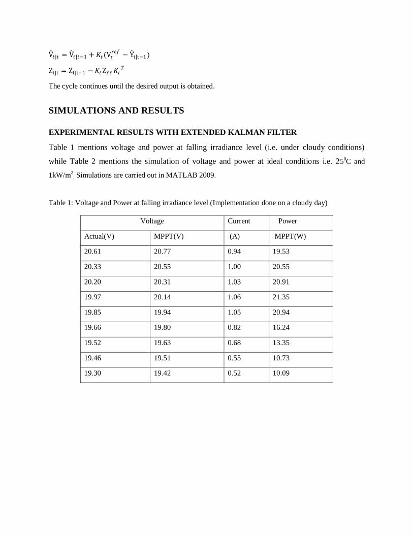
EXPERIMENTAL RESULTS WITH EXTENDED KALMAN FILTER

Table 1 mentions voltage and power at falling irradiance level (i.e. under cloudy conditions)

while Table 2 mentions the simulation of voltage and power at ideal conditions i.e. 250C and

1kW/m2. Simulations are carried out in MATLAB 2009.

Table 1: Voltage and Power at falling irradiance level (Implementation done on a cloudy day)

Voltage Current Power

Actual(V) MPPT(V) (A) MPPT(W)

20.61 20.77 0.94 19.53

20.33 20.55 1.00 20.55

20.20 20.31 1.03 20.91

19.97 20.14 1.06 21.35

19.85 19.94 1.05 20.94

19.66 19.80 0.82 16.24

19.52 19.63 0.68 13.35

19.46 19.51 0.55 10.73

19.30 19.42 0.52 10.09

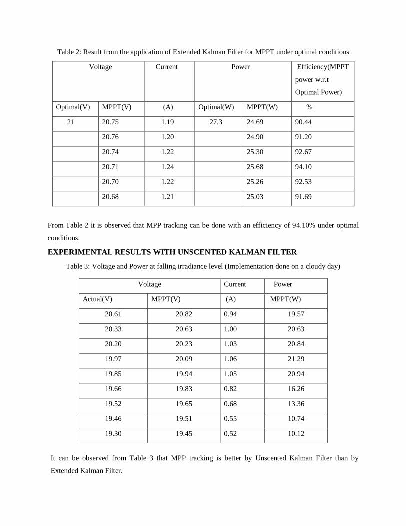
Table 2: Result from the application of Extended Kalman Filter for MPPT under optimal conditions

Voltage Current Power Efficiency(MPPT

power w.r.t

Optimal Power)

Optimal(V) MPPT(V) (A) Optimal(W) MPPT(W) %

21 20.75 1.19 27.3 24.69 90.44

20.76 1.20 24.90 91.20

20.74 1.22 25.30 92.67

20.71 1.24 25.68 94.10

20.70 1.22 25.26 92.53

20.68 1.21 25.03 91.69

From Table 2 it is observed that MPP tracking can be done with an efficiency of 94.10% under optimal

conditions.

EXPERIMENTAL RESULTS WITH UNSCENTED KALMAN FILTER

Table 3: Voltage and Power at falling irradiance level (Implementation done on a cloudy day)

It can be observed from Table 3 that MPP tracking is better by Unscented Kalman Filter than by

Extended Kalman Filter.

Voltage Current Power

Actual(V) MPPT(V) (A) MPPT(W)

20.61 20.82 0.94 19.57

20.33 20.63 1.00 20.63

20.20 20.23 1.03 20.84

19.97 20.09 1.06 21.29

19.85 19.94 1.05 20.94

19.66 19.83 0.82 16.26

19.52 19.65 0.68 13.36

19.46 19.51 0.55 10.74

19.30 19.45 0.52 10.12

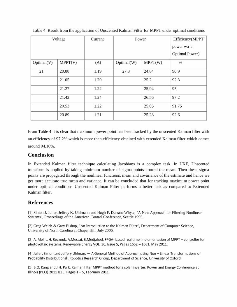
Table 4: Result from the application of Unscented Kalman Filter for MPPT under optimal conditions

Voltage Current Power Efficiency(MPPT

power w.r.t

Optimal Power)

Optimal(V) MPPT(V) (A) Optimal(W) MPPT(W) %

21 20.88 1.19 27.3 24.84 90.9

21.05 1.20 25.2 92.3

21.27 1.22 25.94 95

21.42 1.24 26.56 97.2

20.53 1.22 25.05 91.75

20.89 1.21 25.28 92.6

From Table 4 it is clear that maximum power point has been tracked by the unscented Kalman filter with

an efficiency of 97.2% which is more than efficiency obtained with extended Kalman filter which comes

around 94.10%.

Conclusion

In Extended Kalman filter technique calculating Jacobians is a complex task. In UKF, Unscented

transform is applied by taking minimum number of sigma points around the mean. Then these sigma

points are propagated through the nonlinear functions, mean and covariance of the estimate and hence we

get more accurate true mean and variance. It can be concluded that for tracking maximum power point

under optimal conditions Unscented Kalman Filter performs a better task as compared to Extended

Kalman filter.

References

[1] Simon J. Julier, Jeffrey K. Uhlrnann and Hugh F. Durrant-Whyte, "A New Approach for Filtering Nonlinear Systems", Proceedings of the American Control Conference, Seattle 1995.

[2] Greg Welch & Gary Bishop, "An Introduction to the Kalman Filter", Department of Computer Science,

University of North Carolina at Chapel Hill, July 2006.

[3] A. Mellit, H. Rezzouk, A.Messai, B.Medjahed. FPGA- based real time implementation of MPPT – controller for photovoltaic systems. Renewable Energy VOL. 36, Issue 5, Pages 1652 – 1661, May 2011.

[4] Julier, Simon and Jeffery Uhlman. ― A General Method of Approximating Non – Linear Transformations of Probability Distributions‖. Robotics Research Group, Department of Science, University of Oxford.

[5] B.O. Kang and J.H. Park. Kalman filter MPPT method for a solar inverter. Power and Energy Conference at Illinois (PECI) 2011 IEEE, Pages 1 – 5, February 2011.