digital color reconstruction of a historical film format

Diese Arbeit wurde vorgelegt amLehr- und Forschungsgebiet Informatik 8 (Computer Vision)Fakultat fur Mathematik, Informatik und Naturwissenschaften

Prof. Dr. Bastian Leibe

Master Thesis

Digital color reconstruction of a historicalfilm format

vorgelegt von

Chenfei FanMatrikelnummer: 390189

2020-01-08

Erstgutachter: Prof. Dr. Bastian LeibeZweitgutachter: Prof. Dr. Konrad Schindler

Eidesstattliche Versicherung

Chenfei Fan 390189Name Matrikelnummer

Ich versichere hiermit an Eides Statt, dass ich die vorliegende Masterarbeit mit demTitel

Digital color reconstruction of a historical film format

selbststandig und ohne unzulassige fremde Hilfe erbracht habe. Ich habe keine anderenals die angegebenen Quellen und Hilfsmittel benutzt. Fur den Fall, dass die Arbeitzusatzlich auf einem Datentrager eingereicht wird, erklare ich, dass die schriftlicheund die elektronische Form vollstandig ubereinstimmen. Die Arbeit hat in gleicheroder ahnlicher Form noch keiner Prufungsbehorde vorgelegen.

Aachen, 2020-01-08Ort, Datum Unterschrift

Belehrung:

§ 156 StGB: Falsche Versicherung an Eides StattWer vor einer zur Abnahme einer Versicherung an Eides Statt zuststandigen Behorde eine solcheVersicherung falsch abgibt oder unter Berufung auf eine solche Versicherung falsch aussagt, wirdmit Freiheitsstrafe bis zu drei Jahren oder mit Geldstrafe bestraft.

§ 161 StGB: Fahrlassiger Falscheid; fahrlassige falsche Versicherung an Eides Statt

(1) Wenn eine der in den §§ 154 bis 156 bezeichneten Handlungen aus Fahrlassigkeit begangenworden ist, so tritt Freiheitsstrafe bis zu einem Jahr oder Geldstrafe ein.

(2) Straflosigkeit tritt ein, wenn der Tater die falsche Angabe rechtzeitig berichtigt. Die Vorschriftendes § 158 Abs. 2 und 3 gelten dementsprechend.

Die vorstehende Belehrung habe ich zur Kentnis genommen:

Aachen, 2020-01-08Ort, Datum Unterschrift

iii

Abstract

The lenticular film is a unique color film technique for amateur filmmaking. Themost popular product was released by Kodak in 1928, under the name Kodacolor.Color films produced with this technique provide precious records of everyday lifein the first half of the twentieth century. The film’s surface is engraved with amicroscopic array of cylindrical lenses (the lenticules). Within each lenticule, thecolor of a vertical slice of the image is spatially encoded in grayscale. It requiresa specific projection set-up to regain the color images on the screen. However, wecan also reconstruct the colors from a high-resolution scan of the film materialby digital processing.

As a legacy of the work done in the framework of the doLCE project (Universityof Basel, 2012), the University of Zurich has a software solution to reconstructlenticular colors. The first step of color reconstruction is a precise recognition ofthe boundaries between the lenticules. Its precision suffers from common imper-fections on the film, such as misalignment, defocusing, and noise. Since lenticulesare very narrow, this often leads to false or inconsistent colors in reconstruction.

Inspired by deep learning approaches for a wide range of edge detection tasks, atthe EcoVision Lab, ETH Zurich, we develop a practical lenticule boundary detec-tor using the U-Net architecture. The training dataset is composed of successfulcolor reconstruction results of the doLCE software. Since the training samplesare limited, we use data augmentation methods, such as affine transformationand random erasing, to extend the dataset.

To get even sharper lenticule boundaries, we introduce an iterative approachto refine the recognition results based on the constraint that the width of thelenticules is approximately constant within one image. Without losing muchcolor information, this increases color consistency and speeds up the process ofcolor reconstruction.

Preliminary results of the color reconstruction of the analyzed lenticular filmsshow that the proposed deep learning method improves the result provided by

v

doLCE, reconstructing more truthful and consistent colors.

Keywords: lenticular film, color reconstruction, edge detection

vi

Acknowledgement

I would like to thank Dr. Giorgio Trumpy of University of Zurich for providingme with knowledge in lenticular film and physics about film colors, and prepar-ing the large dataset for training the network. And I would like to thank Dr.Stefano D’Aronco for the thorough supervision and assistance during the thesiswhich helped me to gain knowledge in computer vision and get familiar withPython programming, and the great ideas in color reconstruction. Also thanksto Dr. Joakim Reuteler, Dr. Rudolf Gschwind and AMIA Open Source for thefundamental work on doLCE.

In addition I would like to thank Dr. Jan Dirk Wegner for looking over theproject, and Prof. Konrad Schindler of the Institute of Geodesy and Photogram-metry, ETH Zurich, for providing the resource and funding for my thesis andliving in Zurich. Also thanks to Prof. Bastian Leibe for the recommendation.Finally, I would thank my family for the great support during my study.

vii

Contents

1 Introduction 1

2 Lenticule Detection 72.1 System design . . . . . . . . . . . . . . . . . . . . . . . . . . . . . 8

2.1.1 Model architecture . . . . . . . . . . . . . . . . . . . . . . 92.1.2 Data augmentation . . . . . . . . . . . . . . . . . . . . . . 11

2.2 Training and evaluation . . . . . . . . . . . . . . . . . . . . . . . 112.2.1 Loss . . . . . . . . . . . . . . . . . . . . . . . . . . . . . . 112.2.2 Metrics . . . . . . . . . . . . . . . . . . . . . . . . . . . . 142.2.3 Experiments . . . . . . . . . . . . . . . . . . . . . . . . . . 14

3 Color Reconstruction 173.1 A straightforward implementation . . . . . . . . . . . . . . . . . . 173.2 Reconstruct color by convolution . . . . . . . . . . . . . . . . . . 193.3 Adapt to flexible lenticule widths . . . . . . . . . . . . . . . . . . 23

3.3.1 Soft constraints on widths . . . . . . . . . . . . . . . . . . 243.3.2 Two filters and width mask . . . . . . . . . . . . . . . . . 26

3.4 Color filter design . . . . . . . . . . . . . . . . . . . . . . . . . . . 27

4 Evaluation 294.1 Comparison with doLCE . . . . . . . . . . . . . . . . . . . . . . . 294.2 Discussion . . . . . . . . . . . . . . . . . . . . . . . . . . . . . . . 304.3 conclusion . . . . . . . . . . . . . . . . . . . . . . . . . . . . . . . 32

Bibliography 35

viii

1Introduction

The basic idea of the lenticular film was developed by Raphael Liesegang in 1896,and applied to still photography by Rodolphe Berthon in 1908 [Flu12].

The first commercial lenticular film was marketed by the Eastman Kodak Com-pany in 1928 under the name Kodacolor and provided amateur filmmakers withthe chance of recording everyday life, which serves as precious record of life inthe first half of the twentieth century.

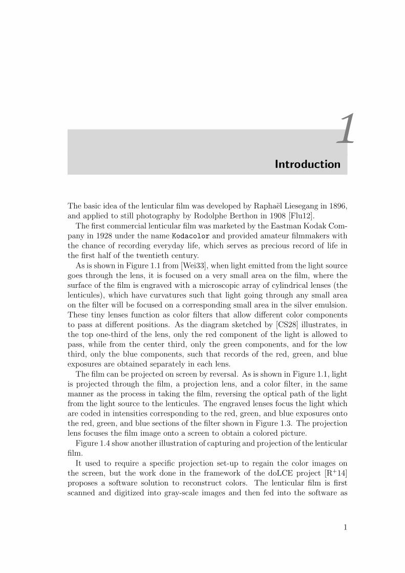
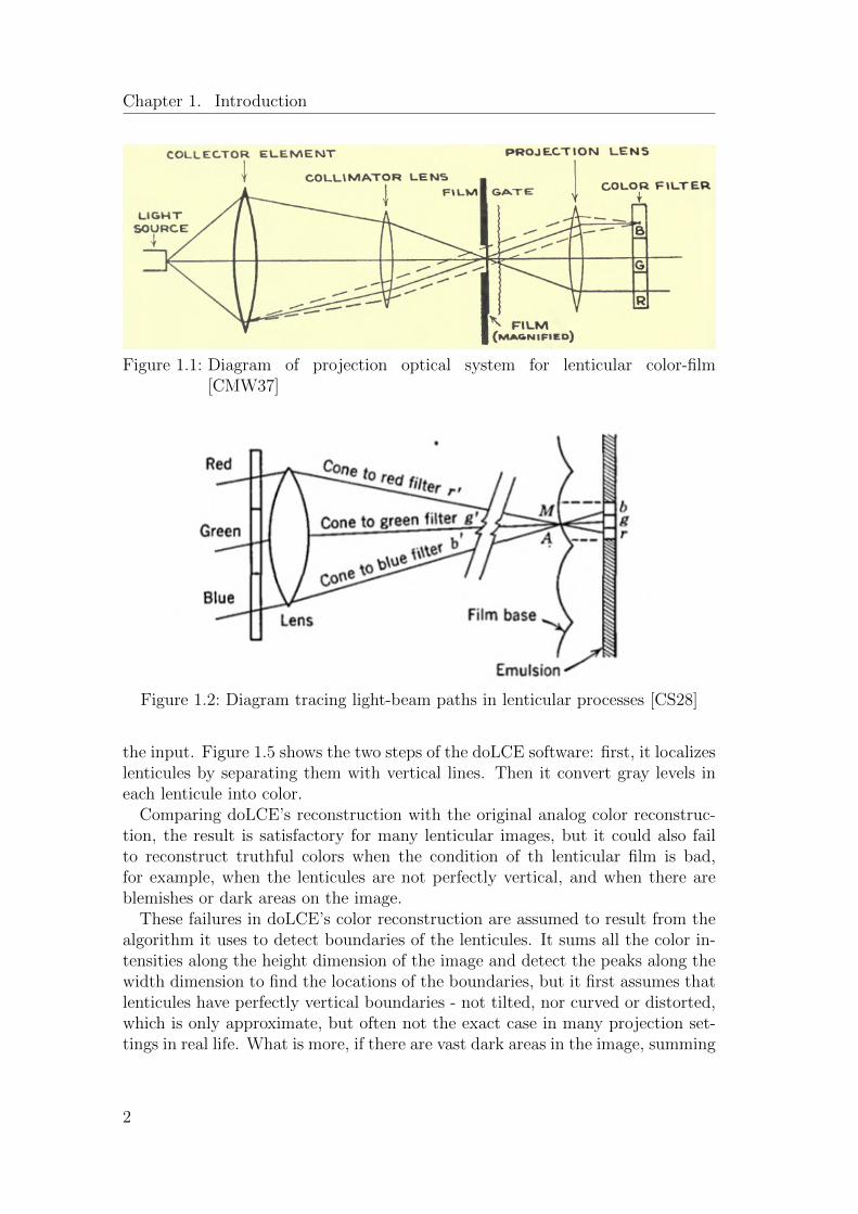
As is shown in Figure 1.1 from [Wei33], when light emitted from the light sourcegoes through the lens, it is focused on a very small area on the film, where thesurface of the film is engraved with a microscopic array of cylindrical lenses (thelenticules), which have curvatures such that light going through any small areaon the filter will be focused on a corresponding small area in the silver emulsion.These tiny lenses function as color filters that allow different color componentsto pass at different positions. As the diagram sketched by [CS28] illustrates, inthe top one-third of the lens, only the red component of the light is allowed topass, while from the center third, only the green components, and for the lowthird, only the blue components, such that records of the red, green, and blueexposures are obtained separately in each lens.

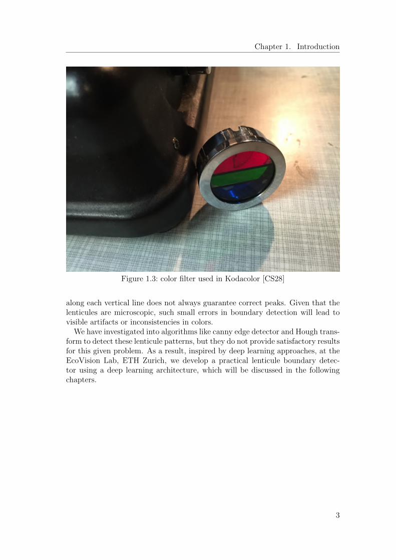
The film can be projected on screen by reversal. As is shown in Figure 1.1, lightis projected through the film, a projection lens, and a color filter, in the samemanner as the process in taking the film, reversing the optical path of the lightfrom the light source to the lenticules. The engraved lenses focus the light whichare coded in intensities corresponding to the red, green, and blue exposures ontothe red, green, and blue sections of the filter shown in Figure 1.3. The projectionlens focuses the film image onto a screen to obtain a colored picture.

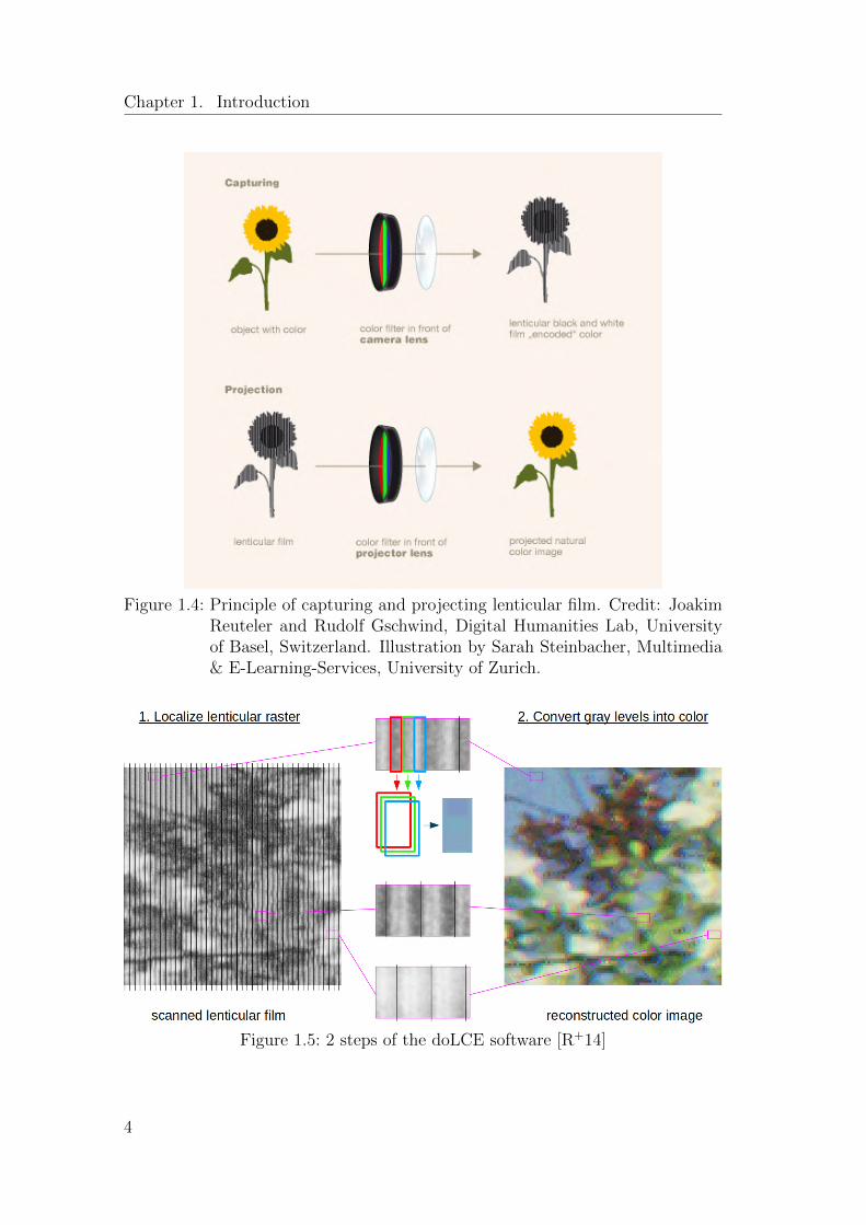
Figure 1.4 show another illustration of capturing and projection of the lenticularfilm.

It used to require a specific projection set-up to regain the color images onthe screen, but the work done in the framework of the doLCE project [R+14]proposes a software solution to reconstruct colors. The lenticular film is firstscanned and digitized into gray-scale images and then fed into the software as

1

Chapter 1. Introduction

Figure 1.1: Diagram of projection optical system for lenticular color-film[CMW37]

Figure 1.2: Diagram tracing light-beam paths in lenticular processes [CS28]

the input. Figure 1.5 shows the two steps of the doLCE software: first, it localizeslenticules by separating them with vertical lines. Then it convert gray levels ineach lenticule into color.

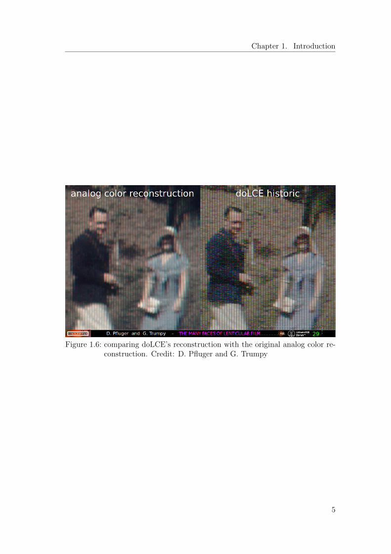
Comparing doLCE’s reconstruction with the original analog color reconstruc-tion, the result is satisfactory for many lenticular images, but it could also failto reconstruct truthful colors when the condition of th lenticular film is bad,for example, when the lenticules are not perfectly vertical, and when there areblemishes or dark areas on the image.

These failures in doLCE’s color reconstruction are assumed to result from thealgorithm it uses to detect boundaries of the lenticules. It sums all the color in-tensities along the height dimension of the image and detect the peaks along thewidth dimension to find the locations of the boundaries, but it first assumes thatlenticules have perfectly vertical boundaries - not tilted, nor curved or distorted,which is only approximate, but often not the exact case in many projection set-tings in real life. What is more, if there are vast dark areas in the image, summing

2


Figure 1.3: color filter used in Kodacolor [CS28]

along each vertical line does not always guarantee correct peaks. Given that thelenticules are microscopic, such small errors in boundary detection will lead tovisible artifacts or inconsistencies in colors.

We have investigated into algorithms like canny edge detector and Hough trans-form to detect these lenticule patterns, but they do not provide satisfactory resultsfor this given problem. As a result, inspired by deep learning approaches, at theEcoVision Lab, ETH Zurich, we develop a practical lenticule boundary detec-tor using a deep learning architecture, which will be discussed in the followingchapters.

3


Figure 1.4: Principle of capturing and projecting lenticular film. Credit: JoakimReuteler and Rudolf Gschwind, Digital Humanities Lab, Universityof Basel, Switzerland. Illustration by Sarah Steinbacher, Multimedia& E-Learning-Services, University of Zurich.

Figure 1.5: 2 steps of the doLCE software [R+14]

4


Figure 1.6: comparing doLCE’s reconstruction with the original analog color re-construction. Credit: D. Pfluger and G. Trumpy

5

2Lenticule Detection

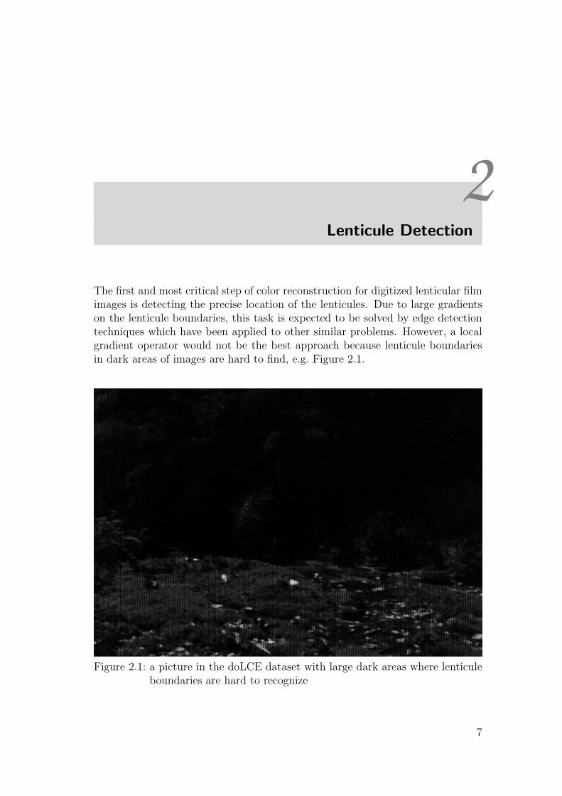
The first and most critical step of color reconstruction for digitized lenticular filmimages is detecting the precise location of the lenticules. Due to large gradientson the lenticule boundaries, this task is expected to be solved by edge detectiontechniques which have been applied to other similar problems. However, a localgradient operator would not be the best approach because lenticule boundariesin dark areas of images are hard to find, e.g. Figure 2.1.

Figure 2.1: a picture in the doLCE dataset with large dark areas where lenticuleboundaries are hard to recognize

7

Chapter 2. Lenticule Detection 2.1. System design

This is where deep learning comes into play. Because lenticule boundaries arevertically continuous, we can guess their unknown parts by extending them fromclearer parts of the image. This requires not only local or neighboring gradientsbut also information from far upper or lower pixels.

2.1 System design

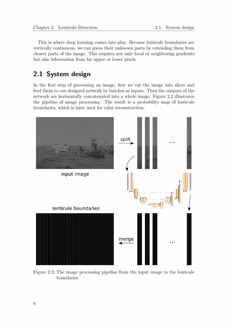
In the first step of processing an image, first we cut the image into slices andfeed them to our designed network by batches as inputs. Then the outputs of thenetwork are horizontally concatenated into a whole image. Figure 2.2 illustratesthe pipeline of image processing. The result is a probability map of lenticuleboundaries, which is later used for color reconstruction.

Figure 2.2: The image processing pipeline from the input image to the lenticuleboundaries

8

2.1. System design Chapter 2. Lenticule Detection

2.1.1 Model architecture

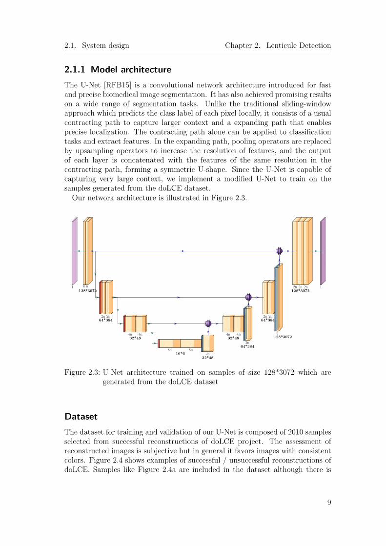
The U-Net [RFB15] is a convolutional network architecture introduced for fastand precise biomedical image segmentation. It has also achieved promising resultson a wide range of segmentation tasks. Unlike the traditional sliding-windowapproach which predicts the class label of each pixel locally, it consists of a usualcontracting path to capture larger context and a expanding path that enablesprecise localization. The contracting path alone can be applied to classificationtasks and extract features. In the expanding path, pooling operators are replacedby upsampling operators to increase the resolution of features, and the outputof each layer is concatenated with the features of the same resolution in thecontracting path, forming a symmetric U-shape. Since the U-Net is capable ofcapturing very large context, we implement a modified U-Net to train on thesamples generated from the doLCE dataset.

Our network architecture is illustrated in Figure 2.3.

1 nn128*3072

2n 2n64*384

4n 4n32*48

8n 8n16*6 4n

32*48

||4n 4n32*48

2n64*384

||

2n 2n64*384

8128*3072

||

2n 2n 2n128*3072

1

Figure 2.3: U-Net architecture trained on samples of size 128*3072 which aregenerated from the doLCE dataset

Dataset

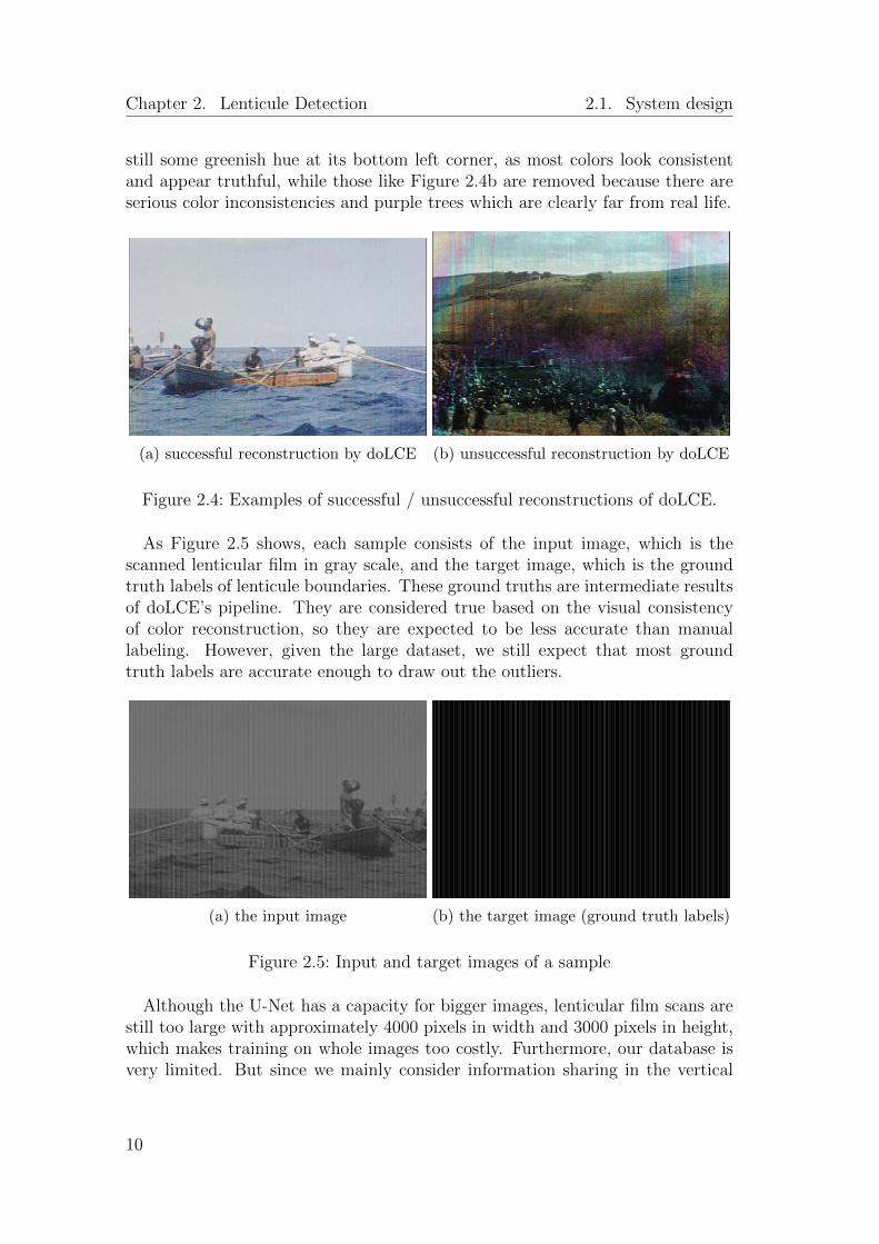
The dataset for training and validation of our U-Net is composed of 2010 samplesselected from successful reconstructions of doLCE project. The assessment ofreconstructed images is subjective but in general it favors images with consistentcolors. Figure 2.4 shows examples of successful / unsuccessful reconstructions ofdoLCE. Samples like Figure 2.4a are included in the dataset although there is

9

Chapter 2. Lenticule Detection 2.1. System design

still some greenish hue at its bottom left corner, as most colors look consistentand appear truthful, while those like Figure 2.4b are removed because there areserious color inconsistencies and purple trees which are clearly far from real life.

(a) successful reconstruction by doLCE (b) unsuccessful reconstruction by doLCE

Figure 2.4: Examples of successful / unsuccessful reconstructions of doLCE.

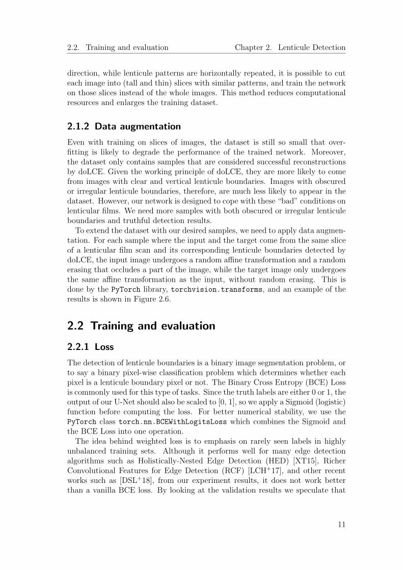
As Figure 2.5 shows, each sample consists of the input image, which is thescanned lenticular film in gray scale, and the target image, which is the groundtruth labels of lenticule boundaries. These ground truths are intermediate resultsof doLCE’s pipeline. They are considered true based on the visual consistencyof color reconstruction, so they are expected to be less accurate than manuallabeling. However, given the large dataset, we still expect that most groundtruth labels are accurate enough to draw out the outliers.

(a) the input image (b) the target image (ground truth labels)

Figure 2.5: Input and target images of a sample

Although the U-Net has a capacity for bigger images, lenticular film scans arestill too large with approximately 4000 pixels in width and 3000 pixels in height,which makes training on whole images too costly. Furthermore, our database isvery limited. But since we mainly consider information sharing in the vertical

10

2.2. Training and evaluation Chapter 2. Lenticule Detection

direction, while lenticule patterns are horizontally repeated, it is possible to cuteach image into (tall and thin) slices with similar patterns, and train the networkon those slices instead of the whole images. This method reduces computationalresources and enlarges the training dataset.

2.1.2 Data augmentation

Even with training on slices of images, the dataset is still so small that over-fitting is likely to degrade the performance of the trained network. Moreover,the dataset only contains samples that are considered successful reconstructionsby doLCE. Given the working principle of doLCE, they are more likely to comefrom images with clear and vertical lenticule boundaries. Images with obscuredor irregular lenticule boundaries, therefore, are much less likely to appear in thedataset. However, our network is designed to cope with these “bad” conditions onlenticular films. We need more samples with both obscured or irregular lenticuleboundaries and truthful detection results.

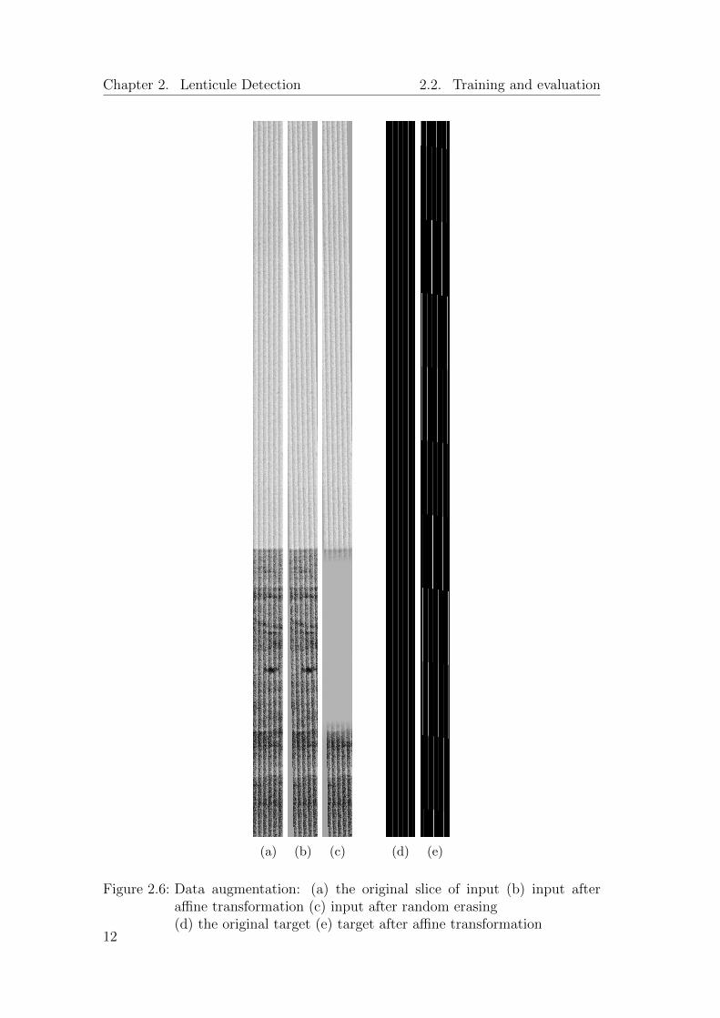
To extend the dataset with our desired samples, we need to apply data augmen-tation. For each sample where the input and the target come from the same sliceof a lenticular film scan and its corresponding lenticule boundaries detected bydoLCE, the input image undergoes a random affine transformation and a randomerasing that occludes a part of the image, while the target image only undergoesthe same affine transformation as the input, without random erasing. This isdone by the PyTorch library, torchvision.transforms, and an example of theresults is shown in Figure 2.6.

2.2 Training and evaluation

2.2.1 Loss

The detection of lenticule boundaries is a binary image segmentation problem, orto say a binary pixel-wise classification problem which determines whether eachpixel is a lenticule boundary pixel or not. The Binary Cross Entropy (BCE) Lossis commonly used for this type of tasks. Since the truth labels are either 0 or 1, theoutput of our U-Net should also be scaled to [0, 1], so we apply a Sigmoid (logistic)function before computing the loss. For better numerical stability, we use thePyTorch class torch.nn.BCEWithLogitsLoss which combines the Sigmoid andthe BCE Loss into one operation.

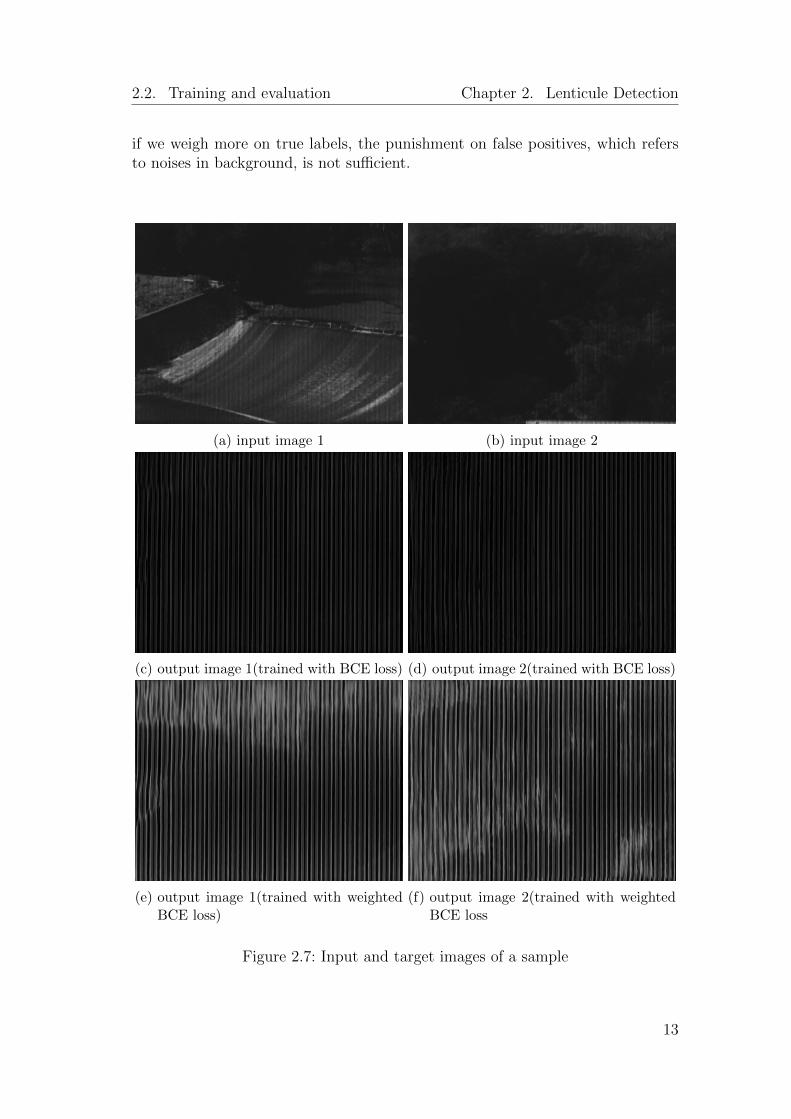
The idea behind weighted loss is to emphasis on rarely seen labels in highlyunbalanced training sets. Although it performs well for many edge detectionalgorithms such as Holistically-Nested Edge Detection (HED) [XT15], RicherConvolutional Features for Edge Detection (RCF) [LCH+17], and other recentworks such as [DSL+18], from our experiment results, it does not work betterthan a vanilla BCE loss. By looking at the validation results we speculate that

11

Chapter 2. Lenticule Detection 2.2. Training and evaluation

(a) (b) (c) (d) (e)

Figure 2.6: Data augmentation: (a) the original slice of input (b) input afteraffine transformation (c) input after random erasing(d) the original target (e) target after affine transformation

12


if we weigh more on true labels, the punishment on false positives, which refersto noises in background, is not sufficient.

(a) input image 1 (b) input image 2

(c) output image 1(trained with BCE loss) (d) output image 2(trained with BCE loss)

(e) output image 1(trained with weightedBCE loss)

(f) output image 2(trained with weightedBCE loss

Figure 2.7: Input and target images of a sample

13


As a result, we use BCE Loss without weights, which trades off recall withprecision. As is shown in Figure 2.7, lenticule boundaries of the validation resultappear to be sharper but also dimmer without training with weighted loss. Al-though we can further fine-tune the weights, as is shown in the next chapter, aconstrained optimization of the lenticule boundaries can compensate the noises,minimizing the impact of different loss functions.

It is worthy noting that only comparing the value of the loss does not helpin choosing the loss function because they are calculated by different criterion.Comparing the output images of the validation sets is always necessary.

2.2.2 Metrics

By deciding on a vanilla BCE Loss function without weights, we have agreedthat precision and recall are equally important for our model. As a result, wemonitor them separately as evaluation metrics, and also calculate dice coeffi-cients [SLV+17], which is commonly used for highly unbalanced segmentations,respectively.

2.2.3 Experiments

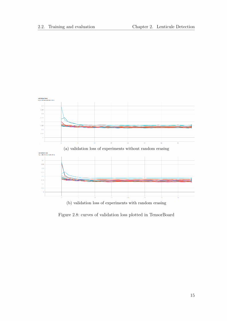
We implement our network using PyTorch and train it on a single NVIDIAGeForce GTX 1080 GPU on the Leonhard cluster provided by ETH Zurich. Weconduct a grid search to find the best setting of parameters. We choose thenumber of features in the first convolutional layer (”n” in Figure 2.3) from {4,8, 16, 32}, the initial learning rate from {0.01, 0.001}, the optimizer from Adam(weight decay=0) and SGD (momentum=0.99), and whether or not to apply ran-dom erasing in data augmentation. By this grid search, we have 32 experimentswith different parameter sets. In each experiment, the network is trained for 40epochs. The learning rate is multiplied by 0.1 after every 7 epochs. The valida-tion losses of these experiments are plotted using TensorBoard. Figure 2.8a andFigure 2.8b show the curves of validation loss of experiments without randomerasing and with random erasing, respectively.

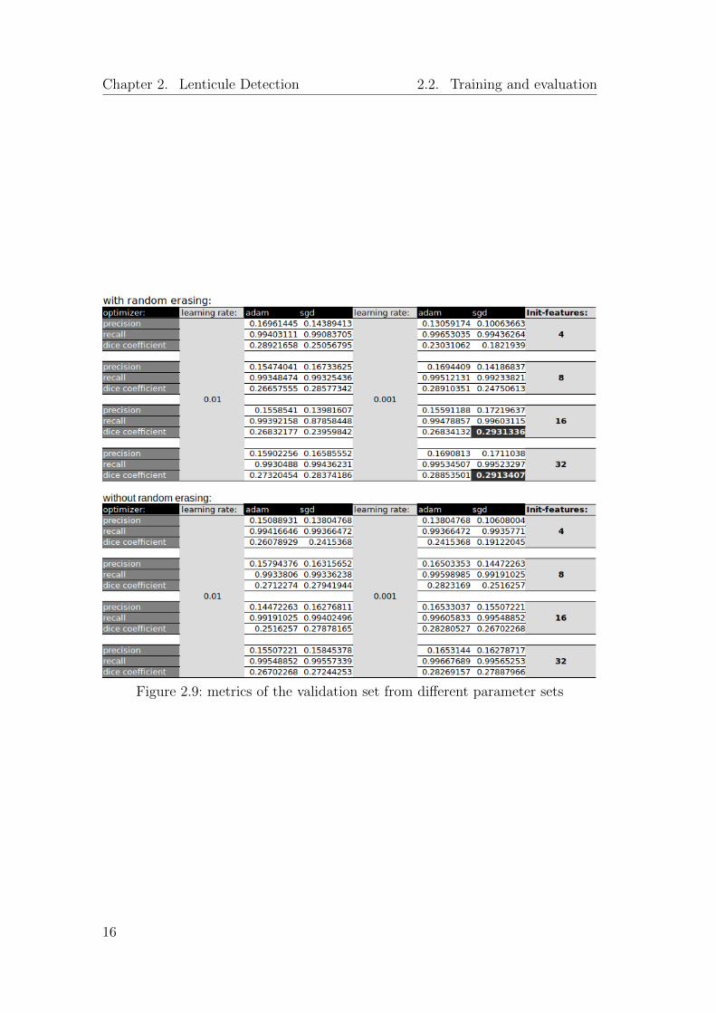
By comparison of validation metrics together with visual outputs, we find thatthe recall is usually satisfactory (for most experiments over 0.99), while the pre-cision, which is only 0.17 in the best case, would determine the sharpness oflenticule boundaries. Therefore we favor the model parameter sets yielding largerprecision.

Contrary to expectation, the curves of loss and metrics do not show a cleartendency with different parameter sets. We choose the parameter set with thelargest dice coefficient (and also the largest precision) shown in Figure 2.9, withrandom erasing in data augmentation, 16 features in the first convolutional layer,an initial learning rate of 0.001, SGD as optimizer, and use this fine-tuned U-Netin Chapter 3 for color reconstruction.

14


(a) validation loss of experiments without random erasing

(b) validation loss of experiments with random erasing

Figure 2.8: curves of validation loss plotted in TensorBoard

15


Figure 2.9: metrics of the validation set from different parameter sets

16

3Color Reconstruction

We speculate that the U-Net architecture proposed in the last chapter providesmore truthful lenticule boundaries, but no conclusion can be drawn until we seethe results of the color reconstruction.

It seems that given the output images of lenticule boundaries, we can alreadyreconstruct color inside each lenticule by following the physics of lenticular filmexplained in Chapter 1. Having a closer look at Figure 1.5, the color of each pixeldepends on the only one row and the only one lenticule it belongs to, so the colorreconstruction can be done by an iteration over each pixel to extract the colorpixel by pixel, though apparently this process could be further optimized.

However, details in implementation are still left to be discussed in this chapter.

3.1 A straightforward implementation

Since color reconstruction is always localized in rows, i.e. we do not consider apixel’s color also depends on its neighbors in adjacent rows, we can reconstructcolor by iterating the same method over rows, where in each iteration we workon a single row of image with 1D ”flat” lenticules.

For a straightforward implementation, the lenticule boundaries are defined suchthat, for one row of the image, if x ∈ [x1, x2] marks one lenticule, then thelenticule to its right needs to satisfy x ∈ [x2 + 1, x3]. Between each two lenticulesthe boundary is sharp, with no gap or overlap.

However, considering the output of the U-Net as a heat map showing the proba-bility of each pixel belonging to the boundary class, we still need a non-maximumsuppression method where only pixels with local maximum probabilities wouldstand out to mark the boundaries of two lenticules. Here we use the methodscipy.signal.find peaks to extract these local maxima. For a better and morestable performance, the required minimal horizontal distance is set to 7.

After extraction of ”sharp” boundaries, the problem is reduced to an inter-polation task inside each lenticule given its left and right boundaries. For ex-

17

Chapter 3. Color Reconstruction 3.1. A straightforward implementation

ample, if x ∈ [x1, x2] marks one lenticule, then its three channels are repre-sented by x ∈ [x1, x1 + (x2 − x1)/3], x ∈ (x1 + (x2 − x1)/3, x2 − (x2 − x1)/3],x ∈ (x2 − (x2 − x1)/3, x2], respectively (conversion from floats to integer pixelvalues are omitted for notation simplicity). Then for each color channel, we canuse, for example, the scipy.interpolate.interp1d method to map the colorintensities in one-third of the whole interval to the whole interval and interpolatethe pixels in between. As is visualized in Figure 1.5, this interpolation stretchesthe three color channels to the full size in width, and then stack them in depth.

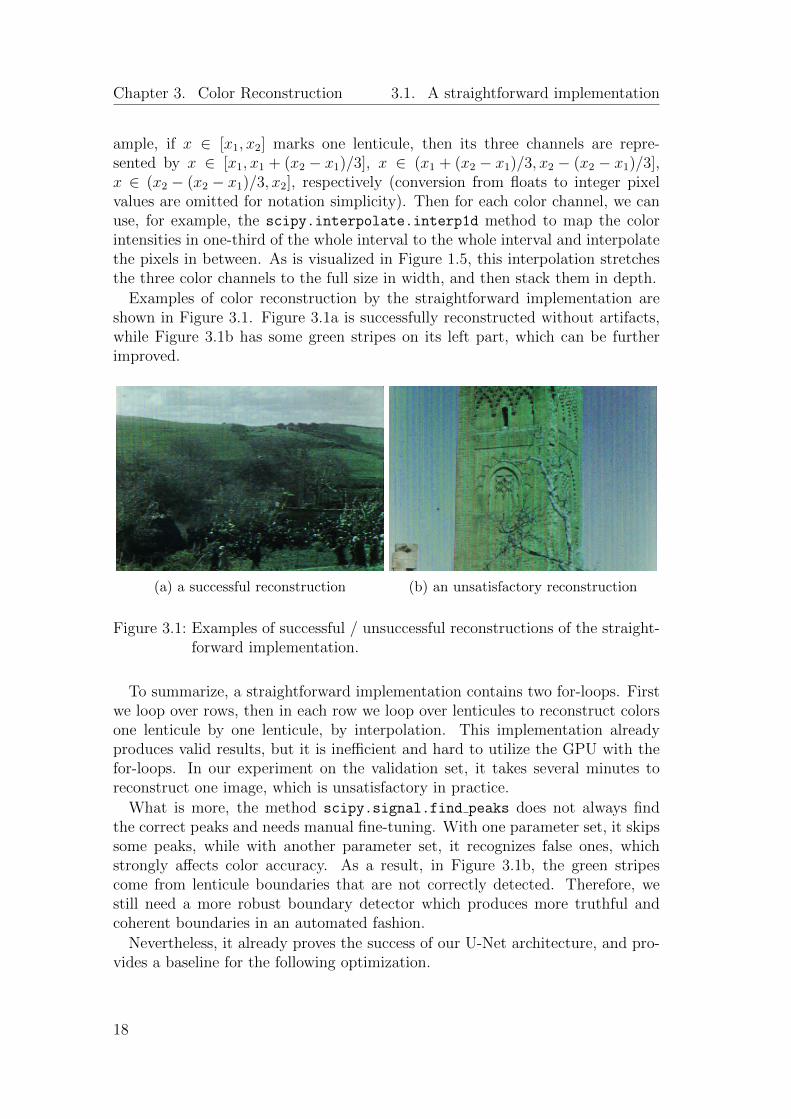
Examples of color reconstruction by the straightforward implementation areshown in Figure 3.1. Figure 3.1a is successfully reconstructed without artifacts,while Figure 3.1b has some green stripes on its left part, which can be furtherimproved.

(a) a successful reconstruction (b) an unsatisfactory reconstruction

Figure 3.1: Examples of successful / unsuccessful reconstructions of the straight-forward implementation.

To summarize, a straightforward implementation contains two for-loops. Firstwe loop over rows, then in each row we loop over lenticules to reconstruct colorsone lenticule by one lenticule, by interpolation. This implementation alreadyproduces valid results, but it is inefficient and hard to utilize the GPU with thefor-loops. In our experiment on the validation set, it takes several minutes toreconstruct one image, which is unsatisfactory in practice.

What is more, the method scipy.signal.find peaks does not always findthe correct peaks and needs manual fine-tuning. With one parameter set, it skipssome peaks, while with another parameter set, it recognizes false ones, whichstrongly affects color accuracy. As a result, in Figure 3.1b, the green stripescome from lenticule boundaries that are not correctly detected. Therefore, westill need a more robust boundary detector which produces more truthful andcoherent boundaries in an automated fashion.

Nevertheless, it already proves the success of our U-Net architecture, and pro-vides a baseline for the following optimization.

18

3.2. Reconstruct color by convolution Chapter 3. Color Reconstruction

3.2 Reconstruct color by convolution

In order to speed up the straightforward implementation of color reconstruction,we need to get rid of the for-loops and replace the interpolation inside for-loopsby a similar but more efficient approach. Since interpolation is related to trans-posed convolution, it is easy to think of applying PyTorch’s built-in convolutionfunctions which are optimized on GPUs, and designing a kernel which mimicsinterpolation.

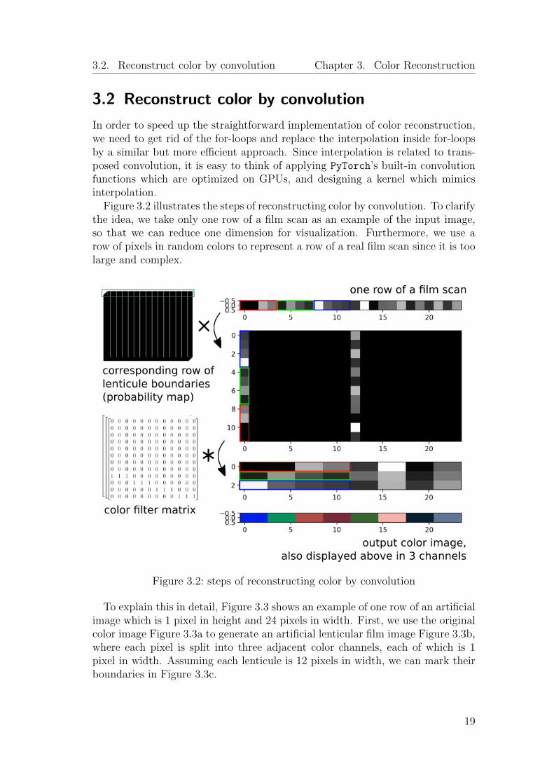
Figure 3.2 illustrates the steps of reconstructing color by convolution. To clarifythe idea, we take only one row of a film scan as an example of the input image,so that we can reduce one dimension for visualization. Furthermore, we use arow of pixels in random colors to represent a row of a real film scan since it is toolarge and complex.

Figure 3.2: steps of reconstructing color by convolution

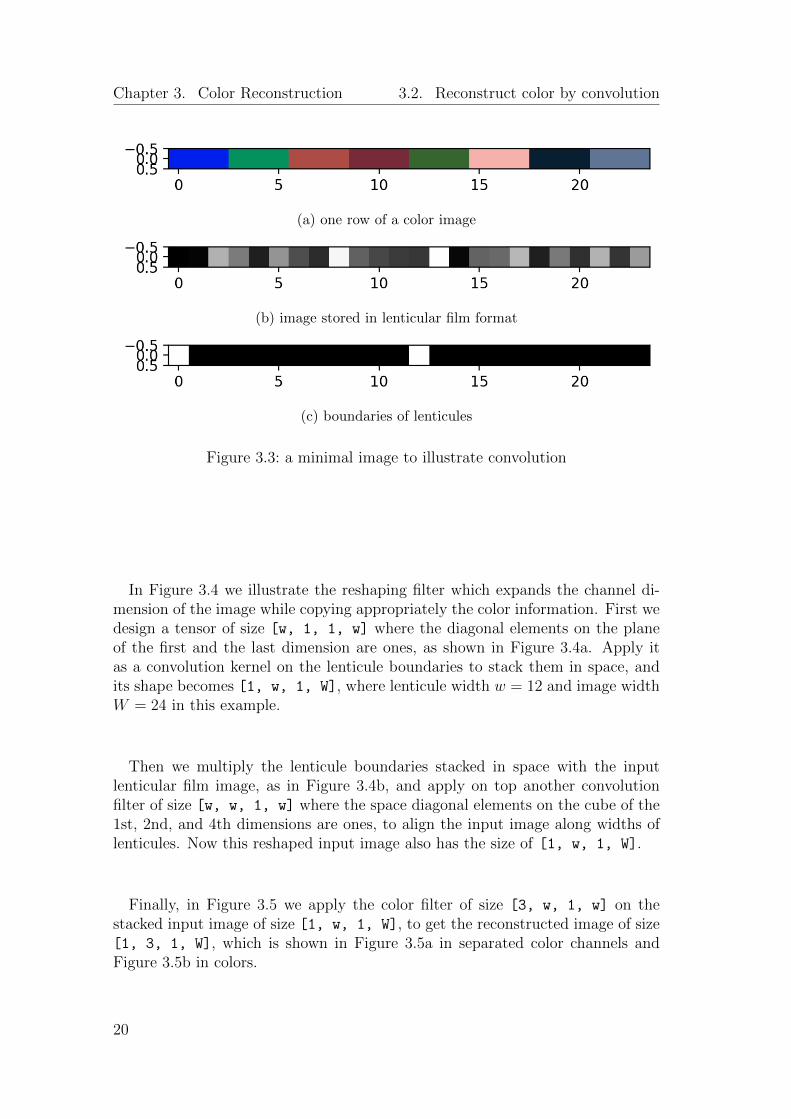
To explain this in detail, Figure 3.3 shows an example of one row of an artificialimage which is 1 pixel in height and 24 pixels in width. First, we use the originalcolor image Figure 3.3a to generate an artificial lenticular film image Figure 3.3b,where each pixel is split into three adjacent color channels, each of which is 1pixel in width. Assuming each lenticule is 12 pixels in width, we can mark theirboundaries in Figure 3.3c.

19

Chapter 3. Color Reconstruction 3.2. Reconstruct color by convolution

(a) one row of a color image

(b) image stored in lenticular film format

(c) boundaries of lenticules

Figure 3.3: a minimal image to illustrate convolution

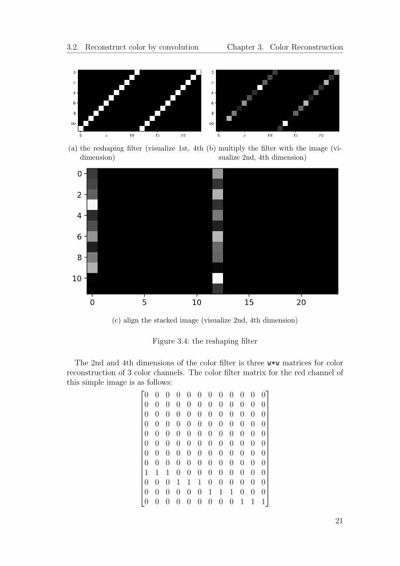
In Figure 3.4 we illustrate the reshaping filter which expands the channel di-mension of the image while copying appropriately the color information. First wedesign a tensor of size [w, 1, 1, w] where the diagonal elements on the planeof the first and the last dimension are ones, as shown in Figure 3.4a. Apply itas a convolution kernel on the lenticule boundaries to stack them in space, andits shape becomes [1, w, 1, W], where lenticule width w = 12 and image widthW = 24 in this example.

Then we multiply the lenticule boundaries stacked in space with the inputlenticular film image, as in Figure 3.4b, and apply on top another convolutionfilter of size [w, w, 1, w] where the space diagonal elements on the cube of the1st, 2nd, and 4th dimensions are ones, to align the input image along widths oflenticules. Now this reshaped input image also has the size of [1, w, 1, W].

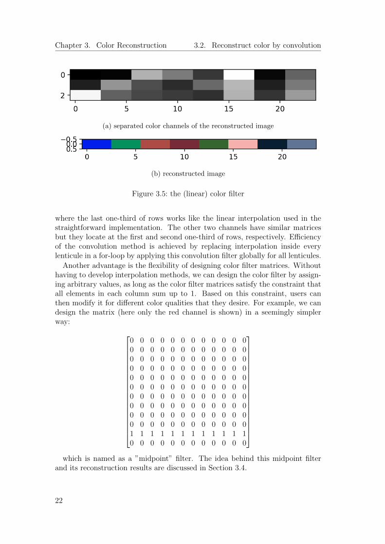
Finally, in Figure 3.5 we apply the color filter of size [3, w, 1, w] on thestacked input image of size [1, w, 1, W], to get the reconstructed image of size[1, 3, 1, W], which is shown in Figure 3.5a in separated color channels andFigure 3.5b in colors.

20

3.2. Reconstruct color by convolution Chapter 3. Color Reconstruction

(a) the reshaping filter (visualize 1st, 4thdimension)

(b) multiply the filter with the image (vi-sualize 2nd, 4th dimension)

(c) align the stacked image (visualize 2nd, 4th dimension)

Figure 3.4: the reshaping filter

The 2nd and 4th dimensions of the color filter is three w*w matrices for colorreconstruction of 3 color channels. The color filter matrix for the red channel ofthis simple image is as follows:

0 0 0 0 0 0 0 0 0 0 0 00 0 0 0 0 0 0 0 0 0 0 00 0 0 0 0 0 0 0 0 0 0 00 0 0 0 0 0 0 0 0 0 0 00 0 0 0 0 0 0 0 0 0 0 00 0 0 0 0 0 0 0 0 0 0 00 0 0 0 0 0 0 0 0 0 0 00 0 0 0 0 0 0 0 0 0 0 01 1 1 0 0 0 0 0 0 0 0 00 0 0 1 1 1 0 0 0 0 0 00 0 0 0 0 0 1 1 1 0 0 00 0 0 0 0 0 0 0 0 1 1 1

21

Chapter 3. Color Reconstruction 3.2. Reconstruct color by convolution

(a) separated color channels of the reconstructed image

(b) reconstructed image

Figure 3.5: the (linear) color filter

where the last one-third of rows works like the linear interpolation used in thestraightforward implementation. The other two channels have similar matricesbut they locate at the first and second one-third of rows, respectively. Efficiencyof the convolution method is achieved by replacing interpolation inside everylenticule in a for-loop by applying this convolution filter globally for all lenticules.

Another advantage is the flexibility of designing color filter matrices. Withouthaving to develop interpolation methods, we can design the color filter by assign-ing arbitrary values, as long as the color filter matrices satisfy the constraint thatall elements in each column sum up to 1. Based on this constraint, users canthen modify it for different color qualities that they desire. For example, we candesign the matrix (here only the red channel is shown) in a seemingly simplerway:

0 0 0 0 0 0 0 0 0 0 0 00 0 0 0 0 0 0 0 0 0 0 00 0 0 0 0 0 0 0 0 0 0 00 0 0 0 0 0 0 0 0 0 0 00 0 0 0 0 0 0 0 0 0 0 00 0 0 0 0 0 0 0 0 0 0 00 0 0 0 0 0 0 0 0 0 0 00 0 0 0 0 0 0 0 0 0 0 00 0 0 0 0 0 0 0 0 0 0 00 0 0 0 0 0 0 0 0 0 0 01 1 1 1 1 1 1 1 1 1 1 10 0 0 0 0 0 0 0 0 0 0 0

which is named as a ”midpoint” filter. The idea behind this midpoint filter

and its reconstruction results are discussed in Section 3.4.

22

3.3. Adapt to flexible lenticule widths Chapter 3. Color Reconstruction

Coherent lenticule boundary corrector

It is important to note that the convolution kernel has a fixed size, where thedimensions of the stack filter and the color filter are equal to the width of thelenticule, namely w in the notation of Section 3.2. However, this is based onthe assumption that all lenticules have the same width in one image, which isnot the case for almost all images. A straightforward solution is to use themode of all distances between peaks to represent the global width of lenticulesof an image. With minor modification, a better formulation is to use the modeof distances between peaks only in the middle row of the image, which is moreefficient. Regardless of which method to use, they both find one integer value thatapproximates all widths of lenticules in an image. As a result, if we apply thesefilters directly to the image, there will be many areas with color inconsistencieswhere the widths of lenticule are not equal to the assumed ”global” width.

To achieve better color coherence in compliance with the convolution kernelsof a fixed size, we develop a pre-processing function to apply on the lenticuleboundary heat map before convolution, where we constrain that all lenticuleshave the same width in one image. This is done by numerical optimization wherethe target is that every w consecutive pixels in one row should sum up to 1,so that for each w consecutive pixels, there is one one pixel belonging to theboundary class. We implement this by applying an all-one convolution kernel ofsize w on the heat map which does the sum, as part of the loss function. At thesame time, the optimized heat map of lenticule boundaries should still be similarto the original one, which is the other part of the loss function. Numericaloptimization is carried out in an iterative manner by built-in optimizers (e.g.torch.optim.Adam) and convolution functions provided by the PyTorch library.

Results show that the new implementation making use of convolution is muchfaster than the straightforward implementation, taking only several seconds foreach image. However, it is based on the assumption that all lenticules have thesame width, which is only true in the ideal condition. Since conditions of filmsvary, this assumption is generally not fulfilled. For images containing a relativelylarge area where lenticule widths are different from those in other areas, it willlead to visual artifacts.

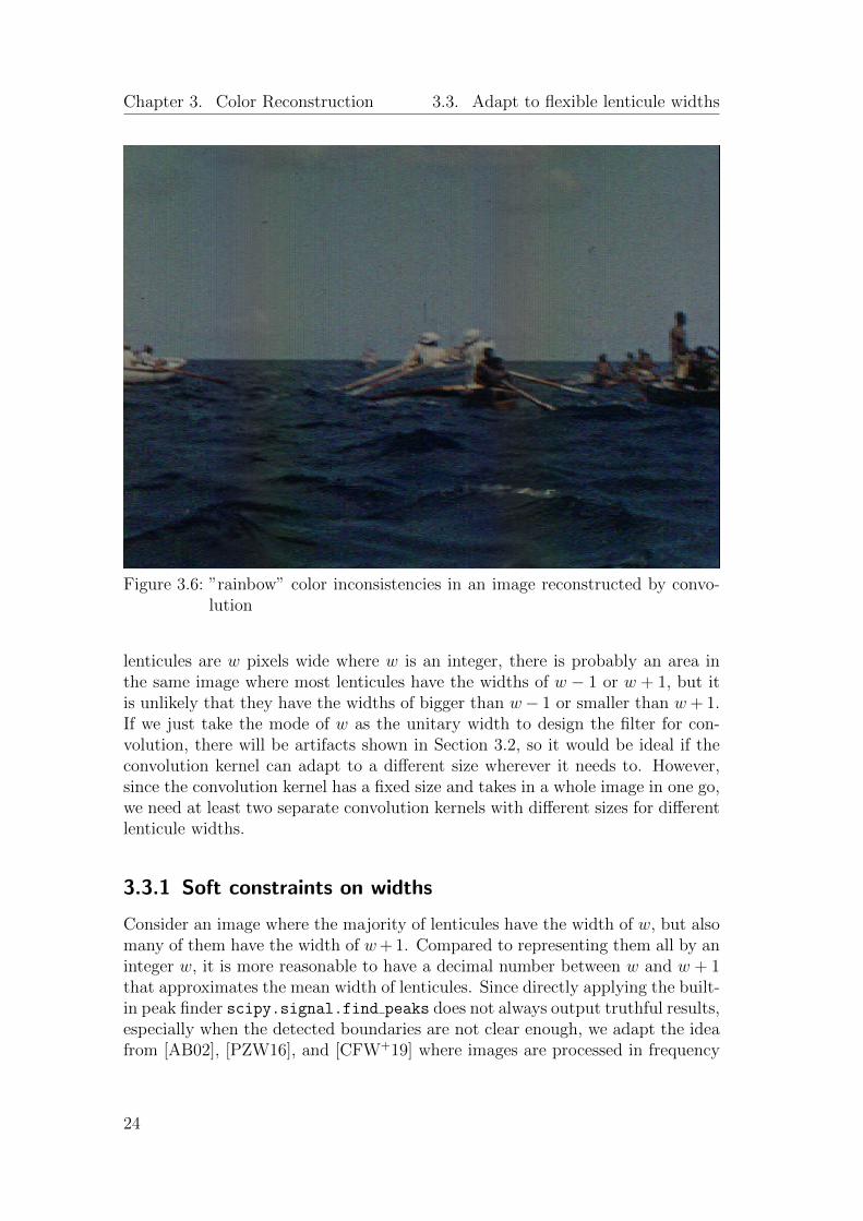
Figure 3.6 shows the limitation of this faster implementation when lenticulewidths vary inside one image. In this case, we need a method that can adaptto different lenticule widths while maintaining the efficiency of the convolutionmethod.

3.3 Adapt to flexible lenticule widths

According to empirical experience provided by the doLCE project, for most lentic-ular films, lenticule widths inside one single image generally have the differenceof no more than one pixel. For example, for an image where the majority of

23

Chapter 3. Color Reconstruction 3.3. Adapt to flexible lenticule widths

Figure 3.6: ”rainbow” color inconsistencies in an image reconstructed by convo-lution

lenticules are w pixels wide where w is an integer, there is probably an area inthe same image where most lenticules have the widths of w − 1 or w + 1, but itis unlikely that they have the widths of bigger than w− 1 or smaller than w + 1.If we just take the mode of w as the unitary width to design the filter for con-volution, there will be artifacts shown in Section 3.2, so it would be ideal if theconvolution kernel can adapt to a different size wherever it needs to. However,since the convolution kernel has a fixed size and takes in a whole image in one go,we need at least two separate convolution kernels with different sizes for differentlenticule widths.

3.3.1 Soft constraints on widths

Consider an image where the majority of lenticules have the width of w, but alsomany of them have the width of w+ 1. Compared to representing them all by aninteger w, it is more reasonable to have a decimal number between w and w + 1that approximates the mean width of lenticules. Since directly applying the built-in peak finder scipy.signal.find peaks does not always output truthful results,especially when the detected boundaries are not clear enough, we adapt the ideafrom [AB02], [PZW16], and [CFW+19] where images are processed in frequency

24

3.3. Adapt to flexible lenticule widths Chapter 3. Color Reconstruction

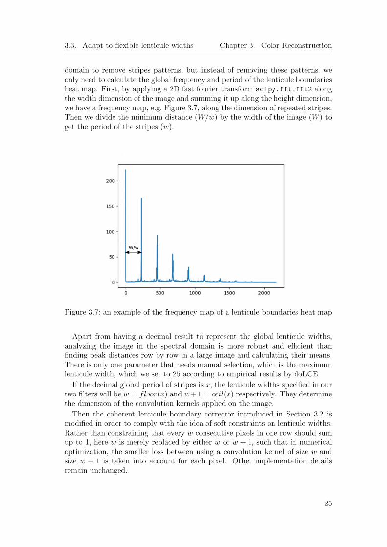
domain to remove stripes patterns, but instead of removing these patterns, weonly need to calculate the global frequency and period of the lenticule boundariesheat map. First, by applying a 2D fast fourier transform scipy.fft.fft2 alongthe width dimension of the image and summing it up along the height dimension,we have a frequency map, e.g. Figure 3.7, along the dimension of repeated stripes.Then we divide the minimum distance (W/w) by the width of the image (W ) toget the period of the stripes (w).

Figure 3.7: an example of the frequency map of a lenticule boundaries heat map

Apart from having a decimal result to represent the global lenticule widths,analyzing the image in the spectral domain is more robust and efficient thanfinding peak distances row by row in a large image and calculating their means.There is only one parameter that needs manual selection, which is the maximumlenticule width, which we set to 25 according to empirical results by doLCE.

If the decimal global period of stripes is x, the lenticule widths specified in ourtwo filters will be w = floor(x) and w+1 = ceil(x) respectively. They determinethe dimension of the convolution kernels applied on the image.

Then the coherent lenticule boundary corrector introduced in Section 3.2 ismodified in order to comply with the idea of soft constraints on lenticule widths.Rather than constraining that every w consecutive pixels in one row should sumup to 1, here w is merely replaced by either w or w + 1, such that in numericaloptimization, the smaller loss between using a convolution kernel of size w andsize w + 1 is taken into account for each pixel. Other implementation detailsremain unchanged.

25

Chapter 3. Color Reconstruction 3.3. Adapt to flexible lenticule widths

3.3.2 Two filters and width mask

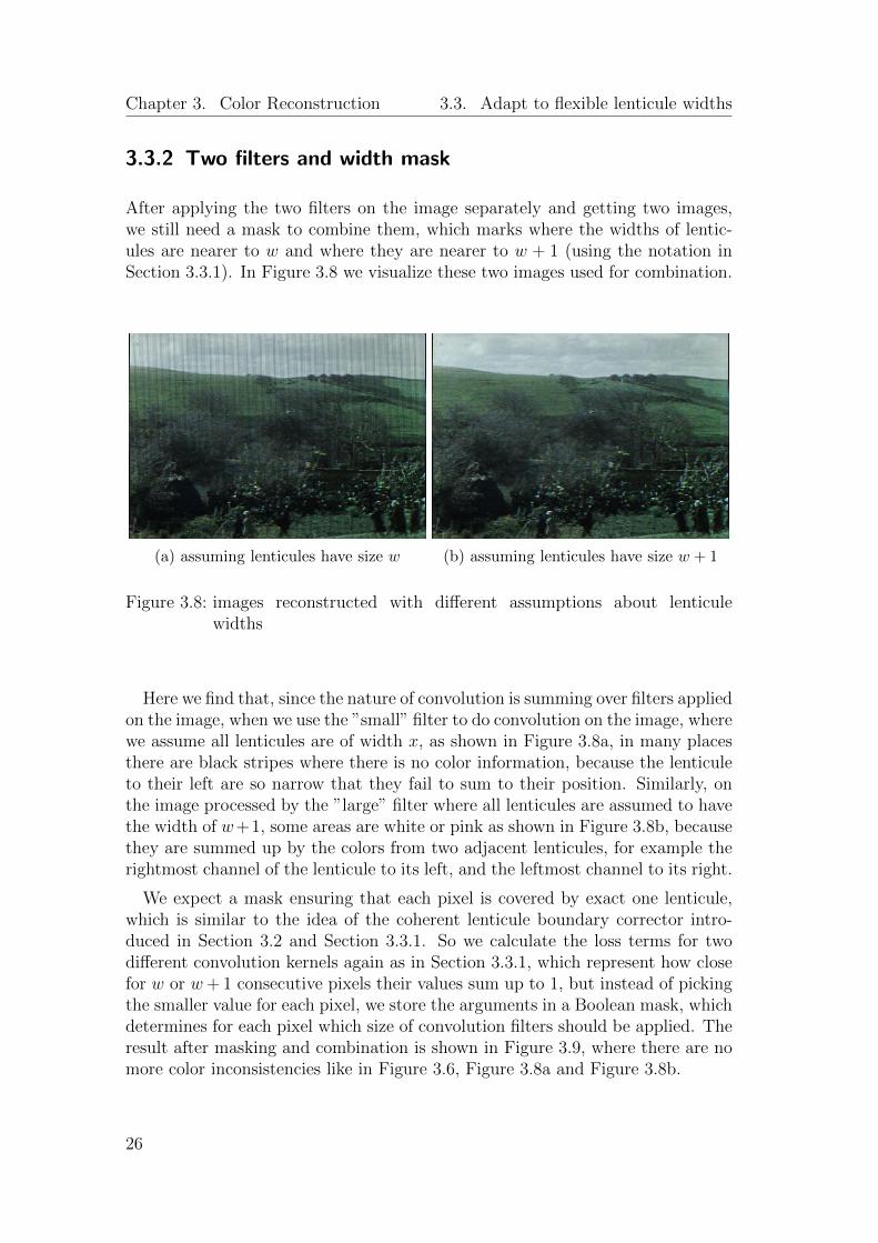
After applying the two filters on the image separately and getting two images,we still need a mask to combine them, which marks where the widths of lentic-ules are nearer to w and where they are nearer to w + 1 (using the notation inSection 3.3.1). In Figure 3.8 we visualize these two images used for combination.

(a) assuming lenticules have size w (b) assuming lenticules have size w + 1

Figure 3.8: images reconstructed with different assumptions about lenticulewidths

Here we find that, since the nature of convolution is summing over filters appliedon the image, when we use the ”small” filter to do convolution on the image, wherewe assume all lenticules are of width x, as shown in Figure 3.8a, in many placesthere are black stripes where there is no color information, because the lenticuleto their left are so narrow that they fail to sum to their position. Similarly, onthe image processed by the ”large” filter where all lenticules are assumed to havethe width of w+1, some areas are white or pink as shown in Figure 3.8b, becausethey are summed up by the colors from two adjacent lenticules, for example therightmost channel of the lenticule to its left, and the leftmost channel to its right.

We expect a mask ensuring that each pixel is covered by exact one lenticule,which is similar to the idea of the coherent lenticule boundary corrector intro-duced in Section 3.2 and Section 3.3.1. So we calculate the loss terms for twodifferent convolution kernels again as in Section 3.3.1, which represent how closefor w or w + 1 consecutive pixels their values sum up to 1, but instead of pickingthe smaller value for each pixel, we store the arguments in a Boolean mask, whichdetermines for each pixel which size of convolution filters should be applied. Theresult after masking and combination is shown in Figure 3.9, where there are nomore color inconsistencies like in Figure 3.6, Figure 3.8a and Figure 3.8b.

26

3.4. Color filter design Chapter 3. Color Reconstruction

Figure 3.9: a successful color reconstruction by combining two filters

3.4 Color filter design

The only detail left to be discussed is the design of color filter. Since even thelenticule boundaries in the original film scan are not precise, there are alwaysambiguity in our detected lenticule boundaries, and also the boundaries betweencolor channels inside one lenticule. As a result, the idea of our default filter is thatwe only pick the pixel at the midpoint of each channel for color reconstruction toavoid misidentifying that a pixel belongs to its neighborhood channel or lenticule.Although it loses some color information, it produces more confident and truthfulcolors. On the other hand, we can also avoid color loss by applying a linearor other smoothed filters if we are very confident about the detected lenticuleboundaries.

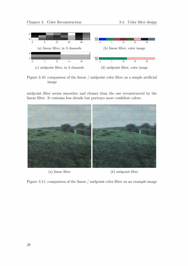
Figure 3.10 show the comparison of colors between applying a linear filter anda midpoint filter on the simple image in Section 3.2. Compare Figure 3.10c toFigure 3.10a, and Figure 3.10b to Figure 3.10d, it is clear that the midpoint filteronly picks the second block of each lenticule to represent the whole lenticule.Although it seems most color information are lost, this idea could be beneficialfor large images.

Figure 3.11 shows the comparison of colors between applying a linear filter anda midpoint filter on an image from the test set. The image reconstructed by the

27

Chapter 3. Color Reconstruction 3.4. Color filter design

(a) linear filter, in 3 channels (b) linear filter, color image

(c) midpoint filter, in 3 channels (d) midpoint filter, color image

Figure 3.10: comparison of the linear / midpoint color filter on a simple artificialimage

midpoint filter seems smoother and cleaner than the one reconstructed by thelinear filter. It contains less details but portrays more confident colors.

(a) linear filter (b) midpoint filter

Figure 3.11: comparison of the linear / midpoint color filter on an example image

28

4Evaluation

4.1 Comparison with doLCE

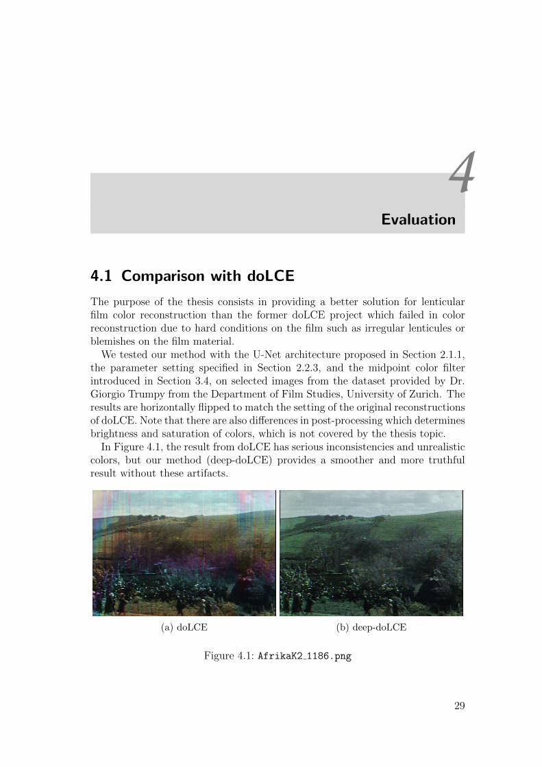
The purpose of the thesis consists in providing a better solution for lenticularfilm color reconstruction than the former doLCE project which failed in colorreconstruction due to hard conditions on the film such as irregular lenticules orblemishes on the film material.

We tested our method with the U-Net architecture proposed in Section 2.1.1,the parameter setting specified in Section 2.2.3, and the midpoint color filterintroduced in Section 3.4, on selected images from the dataset provided by Dr.Giorgio Trumpy from the Department of Film Studies, University of Zurich. Theresults are horizontally flipped to match the setting of the original reconstructionsof doLCE. Note that there are also differences in post-processing which determinesbrightness and saturation of colors, which is not covered by the thesis topic.

In Figure 4.1, the result from doLCE has serious inconsistencies and unrealisticcolors, but our method (deep-doLCE) provides a smoother and more truthfulresult without these artifacts.

(a) doLCE (b) deep-doLCE

Figure 4.1: AfrikaK2 1186.png

29

Chapter 4. Evaluation 4.2. Discussion

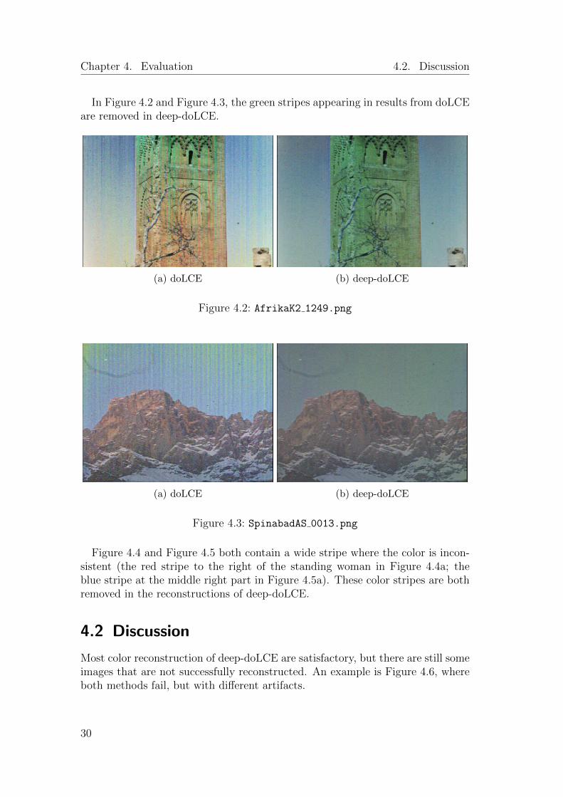
In Figure 4.2 and Figure 4.3, the green stripes appearing in results from doLCEare removed in deep-doLCE.




Figure 4.3: SpinabadAS 0013.png

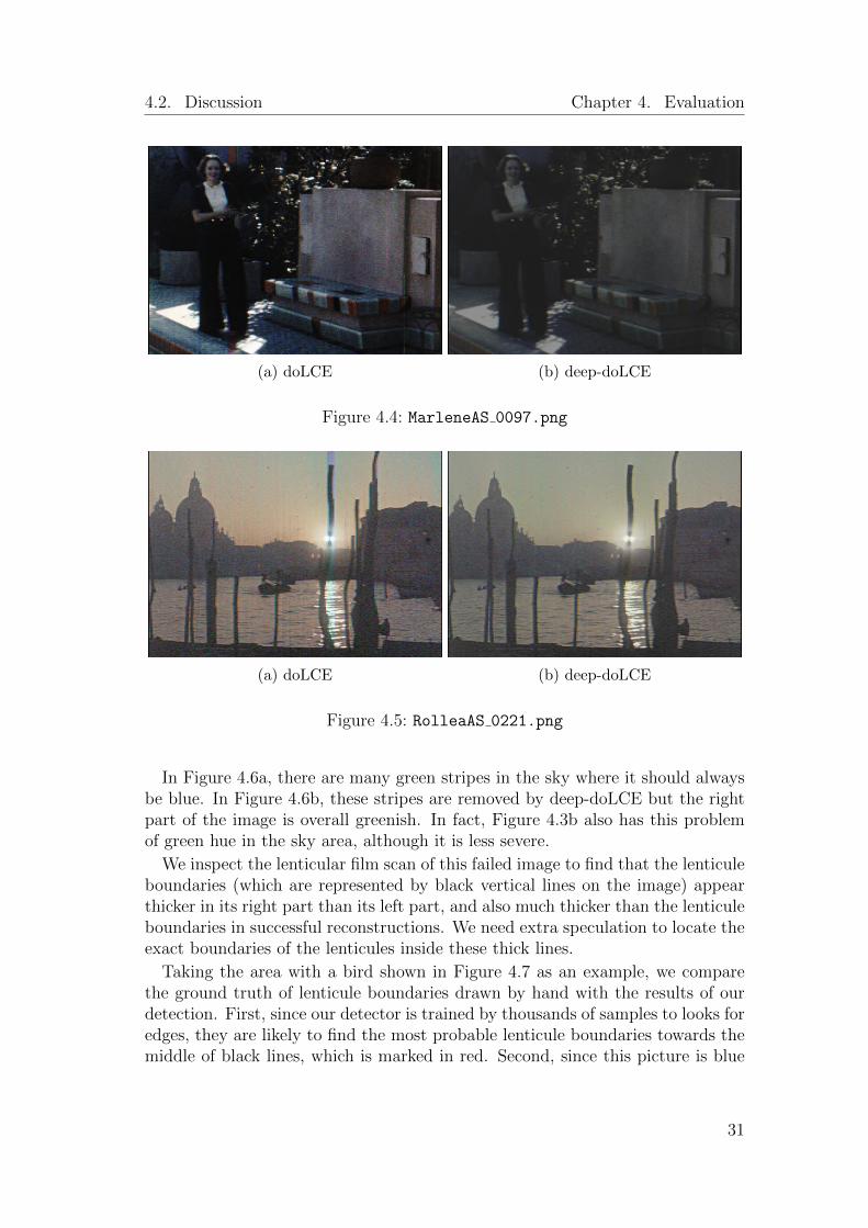
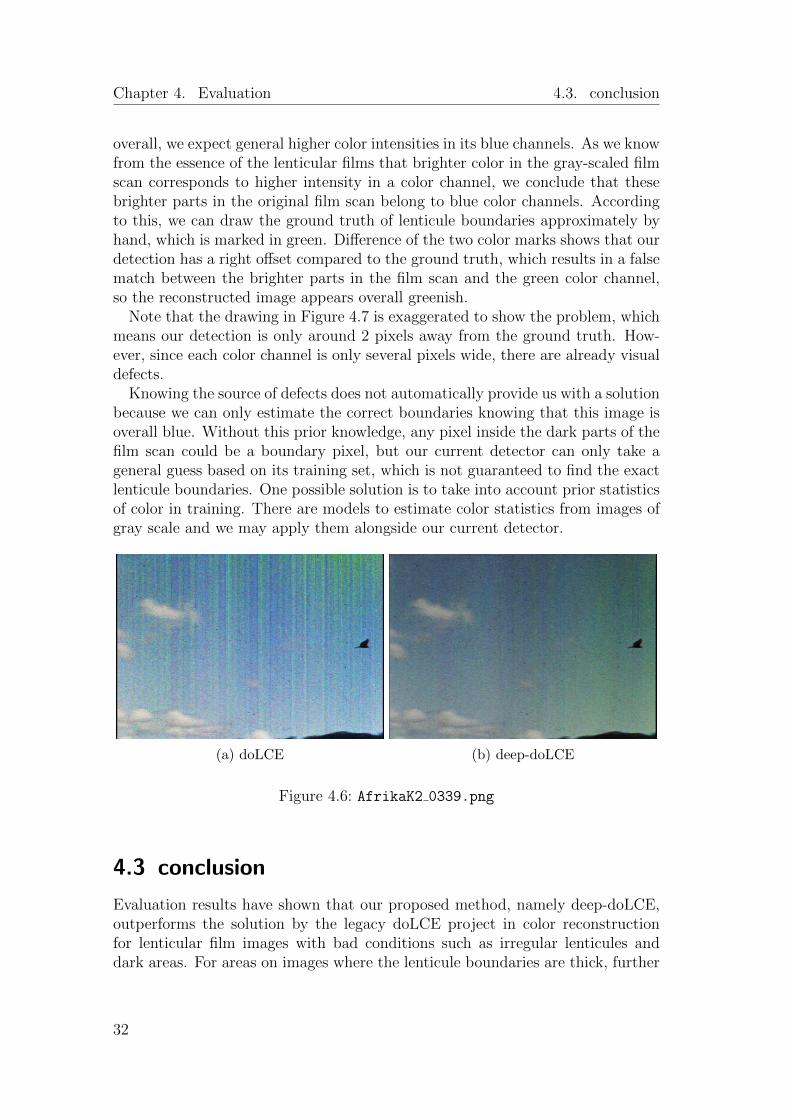
Figure 4.4 and Figure 4.5 both contain a wide stripe where the color is incon-sistent (the red stripe to the right of the standing woman in Figure 4.4a; theblue stripe at the middle right part in Figure 4.5a). These color stripes are bothremoved in the reconstructions of deep-doLCE.

4.2 Discussion

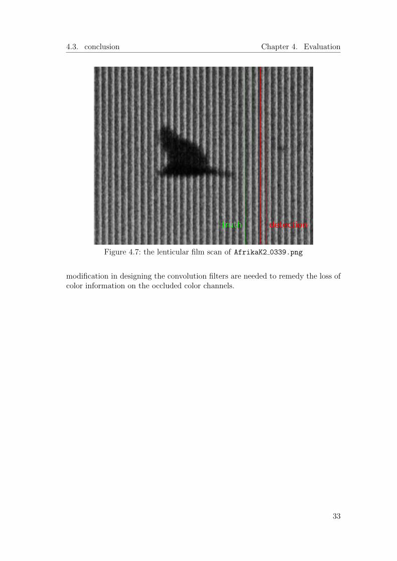
Most color reconstruction of deep-doLCE are satisfactory, but there are still someimages that are not successfully reconstructed. An example is Figure 4.6, whereboth methods fail, but with different artifacts.

30

4.2. Discussion Chapter 4. Evaluation


Figure 4.4: MarleneAS 0097.png


Figure 4.5: RolleaAS 0221.png

In Figure 4.6a, there are many green stripes in the sky where it should alwaysbe blue. In Figure 4.6b, these stripes are removed by deep-doLCE but the rightpart of the image is overall greenish. In fact, Figure 4.3b also has this problemof green hue in the sky area, although it is less severe.

We inspect the lenticular film scan of this failed image to find that the lenticuleboundaries (which are represented by black vertical lines on the image) appearthicker in its right part than its left part, and also much thicker than the lenticuleboundaries in successful reconstructions. We need extra speculation to locate theexact boundaries of the lenticules inside these thick lines.

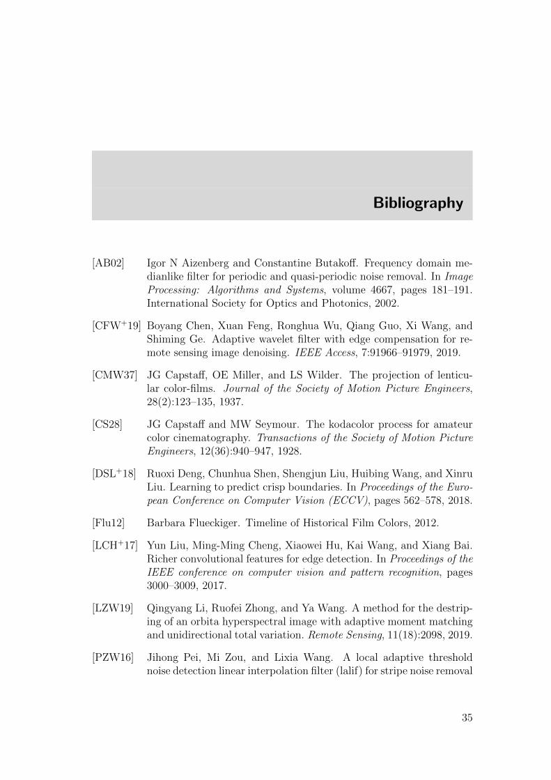
Taking the area with a bird shown in Figure 4.7 as an example, we comparethe ground truth of lenticule boundaries drawn by hand with the results of ourdetection. First, since our detector is trained by thousands of samples to looks foredges, they are likely to find the most probable lenticule boundaries towards themiddle of black lines, which is marked in red. Second, since this picture is blue

31

Chapter 4. Evaluation 4.3. conclusion

overall, we expect general higher color intensities in its blue channels. As we knowfrom the essence of the lenticular films that brighter color in the gray-scaled filmscan corresponds to higher intensity in a color channel, we conclude that thesebrighter parts in the original film scan belong to blue color channels. Accordingto this, we can draw the ground truth of lenticule boundaries approximately byhand, which is marked in green. Difference of the two color marks shows that ourdetection has a right offset compared to the ground truth, which results in a falsematch between the brighter parts in the film scan and the green color channel,so the reconstructed image appears overall greenish.

Note that the drawing in Figure 4.7 is exaggerated to show the problem, whichmeans our detection is only around 2 pixels away from the ground truth. How-ever, since each color channel is only several pixels wide, there are already visualdefects.

Knowing the source of defects does not automatically provide us with a solutionbecause we can only estimate the correct boundaries knowing that this image isoverall blue. Without this prior knowledge, any pixel inside the dark parts of thefilm scan could be a boundary pixel, but our current detector can only take ageneral guess based on its training set, which is not guaranteed to find the exactlenticule boundaries. One possible solution is to take into account prior statisticsof color in training. There are models to estimate color statistics from images ofgray scale and we may apply them alongside our current detector.



4.3 conclusion

Evaluation results have shown that our proposed method, namely deep-doLCE,outperforms the solution by the legacy doLCE project in color reconstructionfor lenticular film images with bad conditions such as irregular lenticules anddark areas. For areas on images where the lenticule boundaries are thick, further

32

4.3. conclusion Chapter 4. Evaluation

Figure 4.7: the lenticular film scan of AfrikaK2 0339.png

modification in designing the convolution filters are needed to remedy the loss ofcolor information on the occluded color channels.

33

Bibliography

[AB02] Igor N Aizenberg and Constantine Butakoff. Frequency domain me-dianlike filter for periodic and quasi-periodic noise removal. In ImageProcessing: Algorithms and Systems, volume 4667, pages 181–191.International Society for Optics and Photonics, 2002.

[CFW+19] Boyang Chen, Xuan Feng, Ronghua Wu, Qiang Guo, Xi Wang, andShiming Ge. Adaptive wavelet filter with edge compensation for re-mote sensing image denoising. IEEE Access, 7:91966–91979, 2019.

[CMW37] JG Capstaff, OE Miller, and LS Wilder. The projection of lenticu-lar color-films. Journal of the Society of Motion Picture Engineers,28(2):123–135, 1937.

[CS28] JG Capstaff and MW Seymour. The kodacolor process for amateurcolor cinematography. Transactions of the Society of Motion PictureEngineers, 12(36):940–947, 1928.

[DSL+18] Ruoxi Deng, Chunhua Shen, Shengjun Liu, Huibing Wang, and XinruLiu. Learning to predict crisp boundaries. In Proceedings of the Euro-pean Conference on Computer Vision (ECCV), pages 562–578, 2018.

[Flu12] Barbara Flueckiger. Timeline of Historical Film Colors, 2012.

[LCH+17] Yun Liu, Ming-Ming Cheng, Xiaowei Hu, Kai Wang, and Xiang Bai.Richer convolutional features for edge detection. In Proceedings of theIEEE conference on computer vision and pattern recognition, pages3000–3009, 2017.

[LZW19] Qingyang Li, Ruofei Zhong, and Ya Wang. A method for the destrip-ing of an orbita hyperspectral image with adaptive moment matchingand unidirectional total variation. Remote Sensing, 11(18):2098, 2019.

[PZW16] Jihong Pei, Mi Zou, and Lixia Wang. A local adaptive thresholdnoise detection linear interpolation filter (lalif) for stripe noise removal

35

Bibliography Bibliography

in infrared images. In 2016 IEEE 13th International Conference onSignal Processing (ICSP), pages 681–686. IEEE, 2016.

[R+14] Joakim Reuteler et al. Die farben des riffelfilms: digitale farbrekon-struktion von linsenrasterfilm. Rundbrief Fotografie, 81:37–41, 2014.

[RFB15] Olaf Ronneberger, Philipp Fischer, and Thomas Brox. U-net: Convo-lutional networks for biomedical image segmentation. In InternationalConference on Medical image computing and computer-assisted inter-vention, pages 234–241. Springer, 2015.

[SLV+17] Carole H Sudre, Wenqi Li, Tom Vercauteren, Sebastien Ourselin, andM Jorge Cardoso. Generalised dice overlap as a deep learning lossfunction for highly unbalanced segmentations. In Deep learning inmedical image analysis and multimodal learning for clinical decisionsupport, pages 240–248. Springer, 2017.

[TDGF18] Giorgio Trumpy, Josephine Diecke, Rudolf Gschwind, and BarbaraFlueckiger. Cyber-digitization: pushing the borders of film restora-tion’s ethic. Electronic Media & Visual Arts, pages 190–195, 2018.

[Wei33] F Weil. The optical-photographic principles of the agfacolor process.Journal of the Society of Motion Picture Engineers, 20(4):301–308,1933.

[XT15] Saining Xie and Zhuowen Tu. Holistically-nested edge detection. InProceedings of the IEEE international conference on computer vision,pages 1395–1403, 2015.

36

digital color reconstruction of a historical film format

Documents