COSMIC RAYS AND THE EARTH’S ATMOSPHERE

A.D. Erlykin1,2 and A.W. Wolfendale2

1 P.N. Lebedev Physics Institute, Leninsky Prospekt, Moscow, Russia.2 Department of Physics, University of Durham, South Road, Durham, DH1 3LE, U.K.

AbstractA very brief summary is given of aspects of cosmic ray physics which have rel-evance to the possible effects of cosmic rays on ‘climate’. It is concluded thata more detailed look at the effect of fast ionizing particles on the atmospherefrom the standpoint of cloud production would be advantageous.

1. INTRODUCTION

There have been many claims for a correlation between solar properties (e.g. sunspot number) and climatebut all have suffered from the absence of a reasonable physical cause, the point being that the energychanges in the solar variations are deemed to be too small to account for the necessary climate forcing.

This is not to say that there are no well-documented effects on very long time scale; there are.Those due to variations in the sun-earth distance and the inclination of the earth’s axis (Milankoviceffects), which relate to 103 − 106 y periods, are generally agreed. What is not (yet) agreed is that the11-year solar cycle has a significant correlation with climate.

The best evidence favouring a specific cause for a sunspot (SS) — climate connection relates tothe apparent role of cosmic rays which are, themselves, modulated by solar activity. The observation isthat by the Danish group in which there is a correlation of cloud cover and CR intensity over the oceans.The likelihood of this being genuine comes from the fact that CR are the major source of ionizationaway from land and CR, of course, provide ionization. Insofar as the cloud cover/CR intensity resultsare considered in detail elsewhere, more discussion will not be given here; rather, we will concentrate onthe CR aspects.

2. COSMIC RAY INTENSITY AS A FUNCTION OF ATMOSPHERIC DEPTH

It is relevant to consider the manner in which the vertical intensity of cosmic rays varies with height inthe atmosphere. Considering the three major components: protons, electrons and muons, the values ofIV , the vertical intensity in cm−2 s−1 sr−1, at heights above sea level of 2, 5 and 10 km, respectively,are:

p : 2 × 10−4, 1.6 × 10−3 and 2 × 10−2

e : 5 × 10−3, 3 × 10−2 and 2 × 10−1

µ : 1 × 10−2, 2 × 10−2 and 5.5 × 10−2.

Some comments can be made, as follows:

(i) The peak of the ionization (for µ and e) is in the 10 km region, much higher than the common cloudlevel. Such an observation is not ‘the kiss of death’ to the correlation idea, because of uncertaintyin transport phenomena for the products of CR ionization between the 10 km level and much lowerlevels.

(ii) Although the ionization produced by protons is lower than that produced by e it is important topoint out that the rare ‘stars’, produced by proton interactions in the atmosphere, contain veryhighly ionizing nuclear fragments. It is not inconceivable that subtle effects leading to clouddroplets are associated with these highly ionizing fragments.

3. KNOWN METEOROLOGICAL EFFECTS

Concerning the CR intensity at ground level there are three major ‘meteorological variations’:

(i) The pressure coefficient, due simply to absorption of the secondaries, of −2% per cm Hg.

(ii) A correlation with the height of the 100 mb level, amounting to ∼ −5% per km. The reason is todo with µ − e decay.

(iii) The mean air temperature between the 100 and 200 mb levels. The dependence is +0.1% perK and is due to π − µ decay.

All the effects are well understood by the cosmic ray fraternity. However, they should be borne inmind by the wider community when correlations are sought.

4. COSMIC RAY ORIGIN — AND EFFECTS

4.1 Galactic particles

Below the ‘knee’ in the energy spectrum, at ∼ 3 × 1015 eV, it is probable that most CR come fromsupernova remnants (SNR) by way of shock acceleration. It is these particles, mainly — specifically,below about 1012 eV — that are modulated by the solar wind which has, itself, an 11-year cycle.

It is inevitable that there should be intensity variations due to the stochastic nature of SNR butthese should be rare. There has been a claim for a 2-fold increase in intensity some 35 thousand yearsago but it seems likely (Beer, private communication) that the increase is due not to an SNR but to avariation of the earth’s magnetic field and/or solar variability.

4.2 Solar particles

With the advent of space vehicles, the study of the (mainly) low energy solar CR has become a ‘growthindustry’. The range-energy relation is such that most protons, or their progeny, do not reach groundlevel; even at 10 GeV the particles only reach a height of about 10 km. Nevertheless, solar CR areimportant, particularly in the polar regions where effects on the ozone layer have been claimed, and theirpresence is eminently reasonable.

Finally, we can remark on the possibility of very rare solar flares having serious effects on climateand, indeed, mankind itself. An extrapolation of the log N − log S curve for energy deposited on earthabove S would indicate very serious effects every million years, or so. However, this interval is surelytoo short (otherwise we would not have survived for so long!). What can be said is that significant effectsmight be expected every 1000 years, or so. Effects on climate might occur if the atmosphere happenedto be in an unstable phase at the time.

5. CONCLUSIONS

Cosmic ray effects offer the possibility of being relevant to climate change. Although it is premature tobe dogmatic, the likelihood of significant climatic effects is high enough for a detailed analysis of thephysics — and meteorology — of CR-air interactions to be not just desirable, but vital.

ACKNOWLEDGEMENTS

The authors are grateful to Jasper Kirkby for re-kindling our interest in this topic.

ICE CORE DATA ON CLIMATE AND COSMIC RAY CHANGES

J. BeerFederal Institute of Environmental Science and Technology, EAWAG, CH-8600 Dübendorf,Switzerland, tel: +41 1 823 51 11 / fax: +41 1 823 52 10, email: beer@eawag.ch

AbstractIce cores represent archives which contain unique information about alarge variety of environmental parameters. Climatic information is storedin the form of stable isotopes, greenhouse gases and various chemicalsubstances. The content of cosmogenic nuclides such as 10Be and 36Clprovide long-term records of the intensity of the cosmic ray flux and itsmodulation by solar activity and the geomagnetic dipole field.Cosmogenic nuclides are produced by the interaction of cosmic rayparticles with the atmosphere. After production, these nuclides aretransported and distributed within the environment, depending on theirgeochemical properties. Some of them are removed from the atmosphereby snow and incorporated into ice sheets and glaciers. The analysis of theGreenland ice cores GRIP and GISP2 are discussed in terms of climateand cosmic ray changes during the past 50’000 years.

1. ARCHIVE ICE

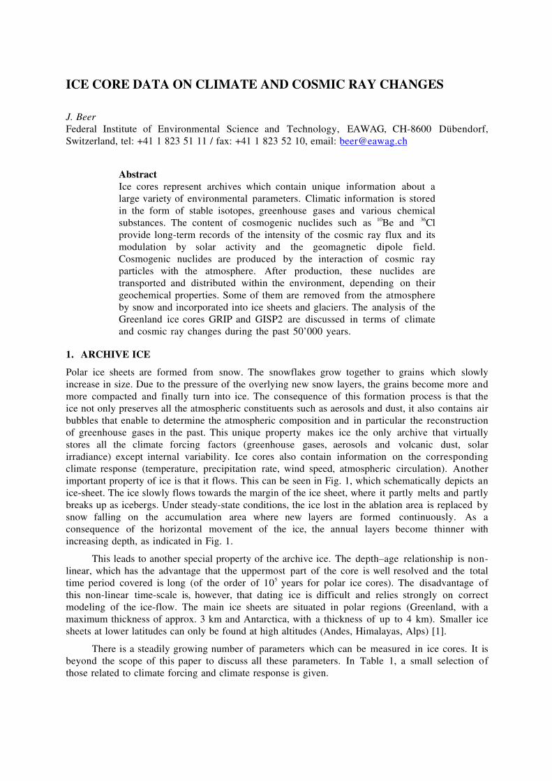
Polar ice sheets are formed from snow. The snowflakes grow together to grains which slowlyincrease in size. Due to the pressure of the overlying new snow layers, the grains become more andmore compacted and finally turn into ice. The consequence of this formation process is that theice not only preserves all the atmospheric constituents such as aerosols and dust, it also contains airbubbles that enable to determine the atmospheric composition and in particular the reconstructionof greenhouse gases in the past. This unique property makes ice the only archive that virtuallystores all the climate forcing factors (greenhouse gases, aerosols and volcanic dust, solarirradiance) except internal variability. Ice cores also contain information on the correspondingclimate response (temperature, precipitation rate, wind speed, atmospheric circulation). Anotherimportant property of ice is that it flows. This can be seen in Fig. 1, which schematically depicts anice-sheet. The ice slowly flows towards the margin of the ice sheet, where it partly melts and partlybreaks up as icebergs. Under steady-state conditions, the ice lost in the ablation area is replaced bysnow falling on the accumulation area where new layers are formed continuously. As aconsequence of the horizontal movement of the ice, the annual layers become thinner withincreasing depth, as indicated in Fig. 1.

This leads to another special property of the archive ice. The depth–age relationship is non-linear, which has the advantage that the uppermost part of the core is well resolved and the totaltime period covered is long (of the order of 105 years for polar ice cores). The disadvantage ofthis non-linear time-scale is, however, that dating ice is difficult and relies strongly on correctmodeling of the ice-flow. The main ice sheets are situated in polar regions (Greenland, with amaximum thickness of approx. 3 km and Antarctica, with a thickness of up to 4 km). Smaller icesheets at lower latitudes can only be found at high altitudes (Andes, Himalayas, Alps) [1].

There is a steadily growing number of parameters which can be measured in ice cores. It isbeyond the scope of this paper to discuss all these parameters. In Table 1, a small selection ofthose related to climate forcing and climate response is given.

BEDROCK

ABLATIONABLATION

ACCUMULATION

Figure 1: Formation of an ice sheet. The snow falling in the accumulation region turns into ice that slowly flows

towards the ablation area where it breaks up into ice-bergs or melts. As a consequence of the flow characteristics the

thickness of annual layers decreases with increasing depth.

Table 1. Climate parameters measured in ice cores.

Parameter Proxy forCO2

CH4

SO4

Ash10Be, 36Cld18OBorehole temperatureAnnual layer thicknessDustAnions / cations

Greenhouse gasesGreenhouse gasesVolcanic eruptionsVolcanic eruptionsSolar activityTemperatureTemperaturePrecipitation rateWind speedAtmospheric circulation

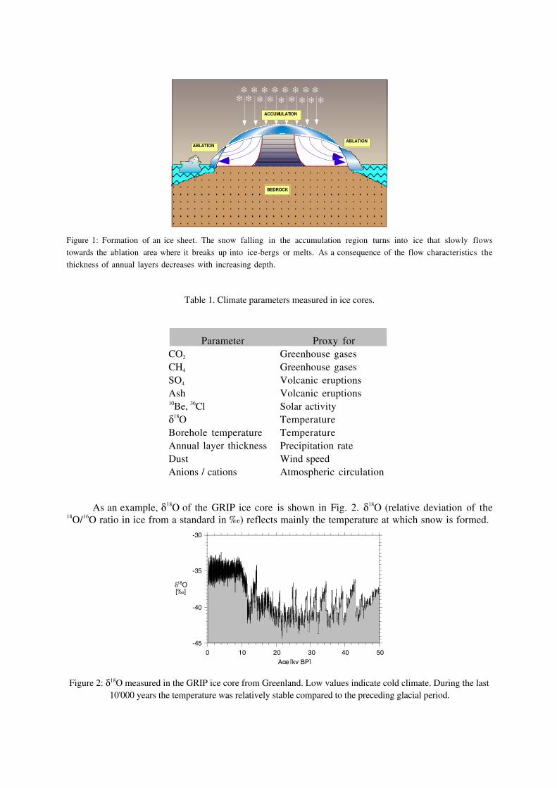
As an example, d18O of the GRIP ice core is shown in Fig. 2. d18O (relative deviation of the18O/16O ratio in ice from a standard in ‰) reflects mainly the temperature at which snow is formed.

-45

-40

-35

-30

0 10 20 30 40 50

d18O[‰]

Age [ky BP]

Figure 2: d18O measured in the GRIP ice core from Greenland. Low values indicate cold climate. During the last10'000 years the temperature was relatively stable compared to the preceding glacial period.

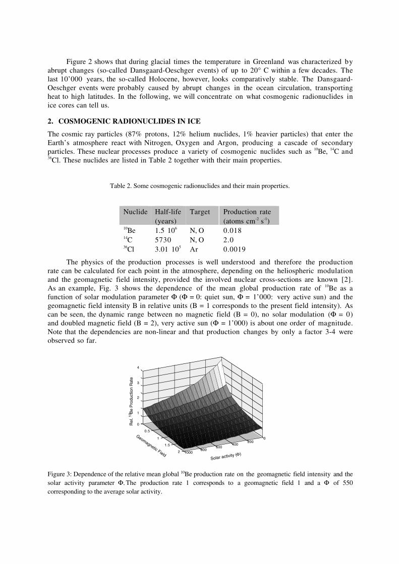
Figure 2 shows that during glacial times the temperature in Greenland was characterized byabrupt changes (so-called Dansgaard-Oeschger events) of up to 20∞ C within a few decades. Thelast 10’000 years, the so-called Holocene, however, looks comparatively stable. The Dansgaard-Oeschger events were probably caused by abrupt changes in the ocean circulation, transportingheat to high latitudes. In the following, we will concentrate on what cosmogenic radionuclides inice cores can tell us.

2. COSMOGENIC RADIONUCLIDES IN ICE

The cosmic ray particles (87% protons, 12% helium nuclides, 1% heavier particles) that enter theEarth’s atmosphere react with Nitrogen, Oxygen and Argon, producing a cascade of secondaryparticles. These nuclear processes produce a variety of cosmogenic nuclides such as 10Be, 14C and36Cl. These nuclides are listed in Table 2 together with their main properties.

Table 2. Some cosmogenic radionuclides and their main properties.

Nuclide Half-life(years)

Target Production rate(atoms cm-2 s-1)

10Be 1.5 106 N, O 0.01814C 5730 N, O 2.036Cl 3.01 105 Ar 0.0019

The physics of the production processes is well understood and therefore the productionrate can be calculated for each point in the atmosphere, depending on the heliospheric modulationand the geomagnetic field intensity, provided the involved nuclear cross-sections are known [2].As an example, Fig. 3 shows the dependence of the mean global production rate of 10Be as afunction of solar modulation parameter F (F = 0: quiet sun, F = 1’000: very active sun) and thegeomagnetic field intensity B in relative units (B = 1 corresponds to the present field intensity). Ascan be seen, the dynamic range between no magnetic field (B = 0), no solar modulation (F = 0)and doubled magnetic field (B = 2), very active sun (F = 1’000) is about one order of magnitude.Note that the dependencies are non-linear and that production changes by only a factor 3-4 wereobserved so far.

0200

400600

8001000

0

0.5

1

1.5

2

1

2

3

4

Solar activity (F)

Geomagnetic Field

Rel

. 10 B

e P

rodu

ctio

n R

ate

Figure 3: Dependence of the relative mean global 10Be production rate on the geomagnetic field intensity and thesolar activity parameter F. The production rate 1 corresponds to a geomagnetic field 1 and a F of 550corresponding to the average solar activity.

The transport of the cosmogenic nuclides produced in the atmosphere is not as wellunderstood as the production processes. 14C forms CO2 and exchanges between the main reservoirsof the carbon cycle (atmosphere, ocean, biosphere). 10Be and 36Cl become attached to aerosols orexist in gaseous form (H36Cl). After a mean residence time of 1 to 2 years they are removed fromthe atmosphere mainly by wet precipitation.

In Polar Regions, the aerosols are removed by the snow that forms the ice sheet. Assuming aproduction rate of 0.018 10Be atoms cm-2 s-1 (Table 2) and a precipitation rate of 100 cm y-1, asimple calculation reveals an average 10Be concentration of approximately 107 atoms per kg of ice.Extremely sensitive detection techniques are necessary to measure 107 atoms. Due to the long half-life, decay counting is not feasible. However, accelerator mass spectrometry (AMS), using singleatom detection is suitable to do the job [3]. A known amount of stable 9Be (typically 0.5 mg) isadded to each sample. This leads to a 10Be/9Be ratio in the range of 10-13 to 10-12. After extraction ofthe Be from the water by ion exchange technique, a BeO sample is produced. This sample is putinto the ion source of the AMS system and an ion beam is produced and accelerated to highenergy (20 MeV) by means of a tandem accelerator. This high energy destroys the molecularbackground and enables suppression of the isobaric background (10B in the case of 10Be). In thefollowing, some of the results obtained so far are discussed:

3. GEOMAGNETIC MODULATION

To reconstruct the geomagnetic field from the 10Be and 36Cl fluxes we assume that the 10Be and 36Clfluxes at Summit are proportional to their average global production rate.

0

0.5

1

1.5

Kgeomagnetic field intensity (deduced from Be-10 andCl-36 data)geomagnetic field intensity(Mediterranean Sea)

Geo

mag

netic

fiel

d in

tens

ity[r

elat

ive

to th

e pr

esen

t lev

el]

Age BP [kyrs]

20 30 40 50 60

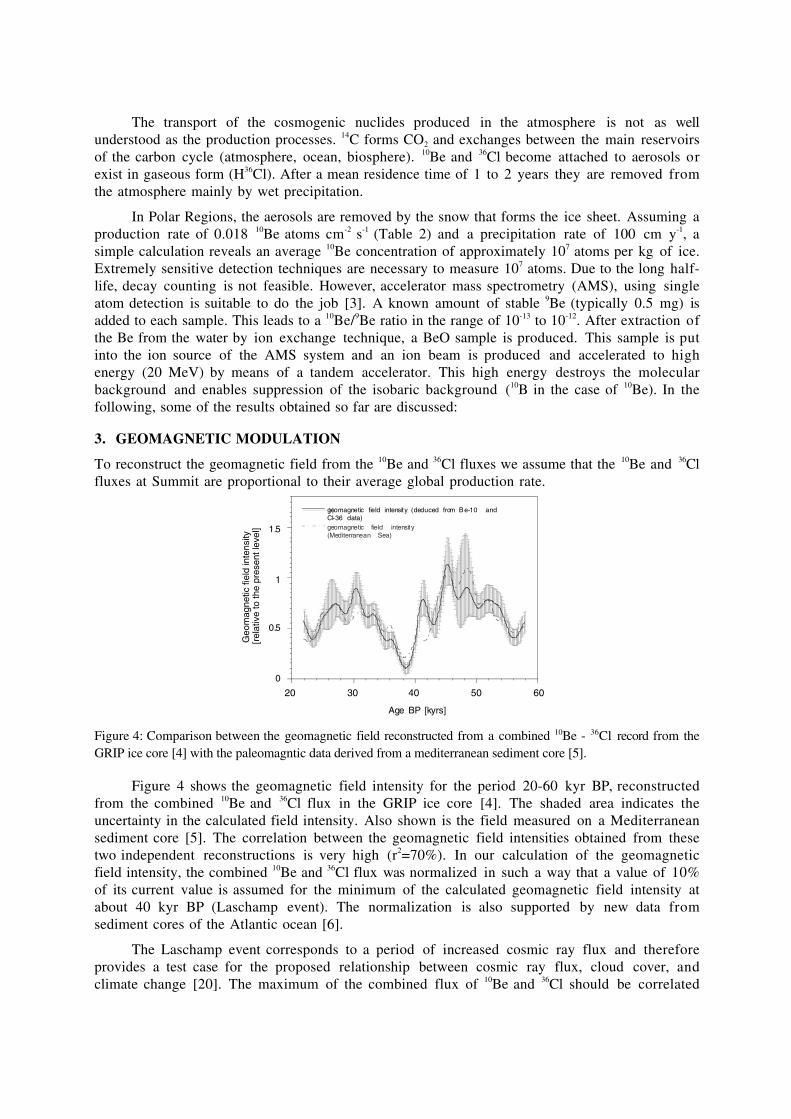
Figure 4: Comparison between the geomagnetic field reconstructed from a combined 10Be - 36Cl record from theGRIP ice core [4] with the paleomagntic data derived from a mediterranean sediment core [5].

Figure 4 shows the geomagnetic field intensity for the period 20-60 kyr BP, reconstructedfrom the combined 10Be and 36Cl flux in the GRIP ice core [4]. The shaded area indicates theuncertainty in the calculated field intensity. Also shown is the field measured on a Mediterraneansediment core [5]. The correlation between the geomagnetic field intensities obtained from thesetwo independent reconstructions is very high (r2=70%). In our calculation of the geomagneticfield intensity, the combined 10Be and 36Cl flux was normalized in such a way that a value of 10%of its current value is assumed for the minimum of the calculated geomagnetic field intensity atabout 40 kyr BP (Laschamp event). The normalization is also supported by new data fromsediment cores of the Atlantic ocean [6].

The Laschamp event corresponds to a period of increased cosmic ray flux and thereforeprovides a test case for the proposed relationship between cosmic ray flux, cloud cover, andclimate change [20]. The maximum of the combined flux of 10Be and 36Cl should be correlated

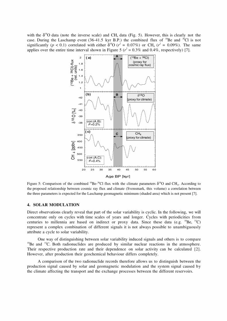
with the d18O data (note the inverse scale) and CH4 data (Fig. 5). However, this is clearly not thecase. During the Laschamp event (36-41.5 kyr B.P.) the combined flux of 10Be and 36Cl is notsignificantly (p < 0.1) correlated with either d18O (r2 = 0.07%) or CH4 (r2 = 0.09%). The sameapplies over the entire time interval shown in Figure 5 (r2 = 0.3% and 0.4%, respectively) [7].

20 25 30 35 40 45 50 55 60

Age BP [kyr]

-42

-41

-40

-39

-38

(10Be + 36Cl)(proxy for

cosmic ray flux)

(proxy for climate)d18O

1.2

1.4

1.6

1.8

A2

(b)

( a)

corr.(A,B):r2=0.2%

B

350

550

450

(proxy for climate)CH4

400

500

C

corr.(A,C):r2=0.4%

( c)

1

CH4

[ppb

v]d18

O [‰

](1

0 Be

+ 36

Cl)-

flux

(rel

. uni

ts)

Figure 5: Comparison of the combined 10Be-36Cl flux with the climate parameters d18O and CH4. According tothe proposed relationship between cosmic ray flux and climate (Svensmark, this volume) a correlation betweenthe three parameters is expected for the Laschamp geomagnetic minimum (shaded area) which is not present [7].

4. SOLAR MODULATION

Direct observations clearly reveal that part of the solar variability is cyclic. In the following, we willconcentrate only on cycles with time scales of years and longer. Cycles with periodicities fromcenturies to millennia are based on indirect or proxy data. Since these data (e.g. 10Be, 14C)represent a complex combination of different signals it is not always possible to unambiguouslyattribute a cycle to solar variability.

One way of distinguishing between solar variability induced signals and others is to compare10Be and 14C. Both radionuclides are produced by similar nuclear reactions in the atmosphere.Their respective production rate and their dependence on solar activity can be calculated [2].However, after production their geochemical behaviour differs completely.

A comparison of the two radionuclide records therefore allows us to distinguish between theproduction signal caused by solar and geomagnetic modulation and the system signal caused bythe climate affecting the transport and the exchange processes between the different reservoirs.

The results from such comparisons indicate that, for the past several millennia, the short-term (decades to centuries) fluctuations in the D14C record are mainly due to production variations,most probably caused by solar modulation.

It is important to note that cycles associated with solar activity do not have a fixedperiodicity. For example in the case of the sunspot cycle, the periodicity varies between 9 and 17years. This raises the important question whether the periodicity averaged over longer timesremains constant or not [8, 9]. To answer this question, longer and very precisely dated records ofsolar activity are needed than are presently available.

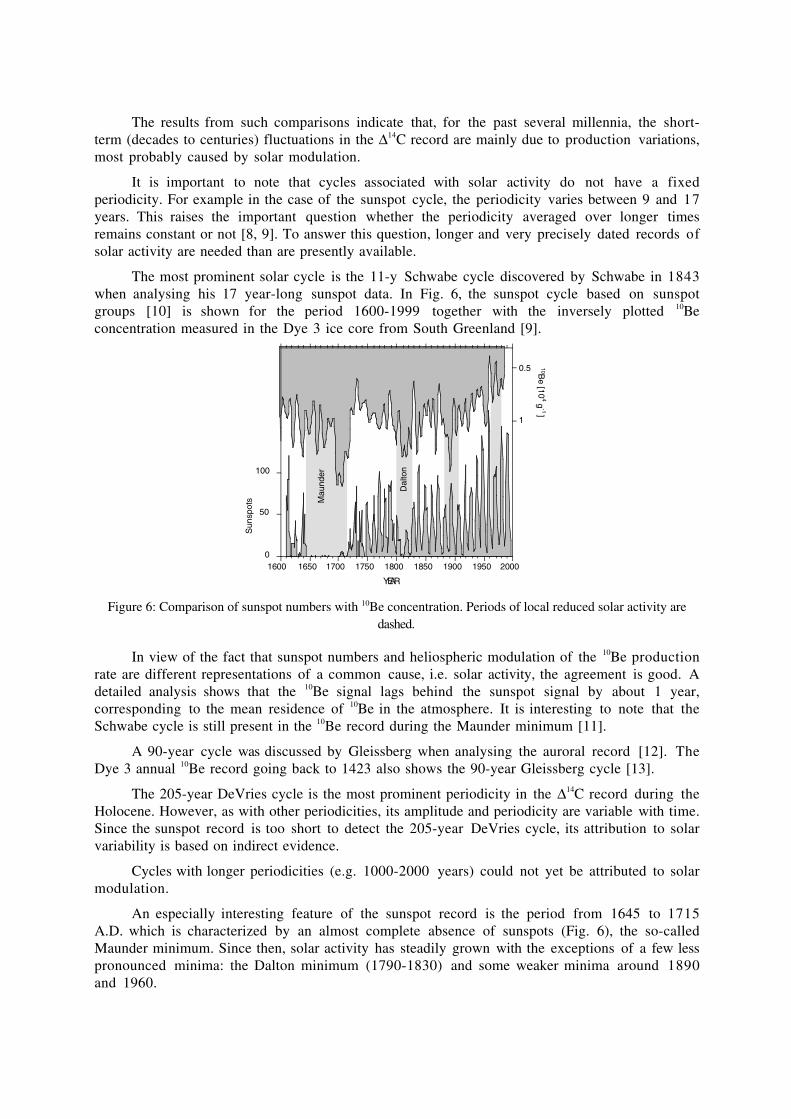
The most prominent solar cycle is the 11-y Schwabe cycle discovered by Schwabe in 1843when analysing his 17 year-long sunspot data. In Fig. 6, the sunspot cycle based on sunspotgroups [10] is shown for the period 1600-1999 together with the inversely plotted 10Beconcentration measured in the Dye 3 ice core from South Greenland [9].

0

50

100

0.5

1

1600 1650 1700 1750 1800 1850 1900 1950 2000

Sun

spot

s10B

e [104 g

-1]

YEAR

Mau

nder

Dal

ton

Figure 6: Comparison of sunspot numbers with 10Be concentration. Periods of local reduced solar activity aredashed.

In view of the fact that sunspot numbers and heliospheric modulation of the 10Be productionrate are different representations of a common cause, i.e. solar activity, the agreement is good. Adetailed analysis shows that the 10Be signal lags behind the sunspot signal by about 1 year,corresponding to the mean residence of 10Be in the atmosphere. It is interesting to note that theSchwabe cycle is still present in the 10Be record during the Maunder minimum [11].

A 90-year cycle was discussed by Gleissberg when analysing the auroral record [12]. TheDye 3 annual 10Be record going back to 1423 also shows the 90-year Gleissberg cycle [13].

The 205-year DeVries cycle is the most prominent periodicity in the D14C record during theHolocene. However, as with other periodicities, its amplitude and periodicity are variable with time.Since the sunspot record is too short to detect the 205-year DeVries cycle, its attribution to solarvariability is based on indirect evidence.

Cycles with longer periodicities (e.g. 1000-2000 years) could not yet be attributed to solarmodulation.

An especially interesting feature of the sunspot record is the period from 1645 to 1715A.D. which is characterized by an almost complete absence of sunspots (Fig. 6), the so-calledMaunder minimum. Since then, solar activity has steadily grown with the exceptions of a few lesspronounced minima: the Dalton minimum (1790-1830) and some weaker minima around 1890and 1960.

-20

-10

0

10

20

30

40

01000200030004000500060007000

Year BPD

14C

[‰]

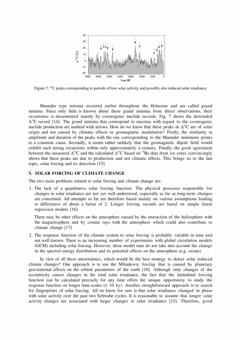
Figure 7: 14C peaks corresponding to periods of low solar activity and possibly also reduced solar irradiance

Maunder type minima occurred earlier throughout the Holocene and are called grandminima. Since only little is known about these grand minima from direct observations, theiroccurrence is documented mainly by cosmogenic nuclide records. Fig. 7 shows the detrendedD14C record [14]: The grand minima that correspond to maxima with regard to the cosmogenicnuclide production are marked with arrows. How do we know that these peaks in D14C are of solarorigin and not caused by climatic effects or geomagnetic modulation? Firstly, the similarity inamplitude and duration of the peaks with the one corresponding to the Maunder minimum pointsto a common cause. Secondly, it seems rather unlikely that the geomagnetic dipole field wouldexhibit such strong excursions within only approximately a century. Finally, the good agreementbetween the measured D14C and the calculated D14C based on 10Be data from ice cores convincinglyshows that these peaks are due to production and not climatic effects. This brings us to the lasttopic, solar forcing and its detection [15].

5. SOLAR FORCING OF CLIMATE CHANGE

The two main problems related to solar forcing and climate change are:

1. The lack of a quantitative solar forcing function. The physical processes responsible forchanges in solar irradiance are not yet well understood, especially as far as long-term changesare concerned. All attempts so far are therefore based mainly on various assumptions leadingto differences of about a factor of 2. Longer forcing records are based on simple linearregression models [16].

There may be other effects on the atmosphere caused by the interaction of the heliosphere withthe magnetosphere and by cosmic rays with the atmosphere which could also contribute toclimate change [17].

2. The response function of the climate system to solar forcing is probably variable in time andnot well known. There is an increasing number of experiments with global circulation models(GCM) including solar forcing. However, these model runs do not take into account the changein the spectral energy distribution and its potential effects on the atmosphere (e.g. ozone).

In view of all these uncertainties, which would be the best strategy to detect solar inducedclimate changes? One approach is to use the Milankovic forcing that is caused by planetarygravitational effects on the orbital parameters of the earth [18]. Although only changes of theeccentricity causes changes in the total solar irradiance, the fact that the latitudinal forcingfunction can be calculated precisely for any time offers the unique opportunity to study theresponse function on longer time-scales (≥ 10 ky). Another straightforward approach is to searchfor fingerprints of solar forcing. All we know for sure is that solar irradiance changed in phasewith solar activity over the past two Schwabe cycles. It is reasonable to assume that longer solaractivity changes are associated with larger changes in solar irradiance [15]. Therefore, good

candidates for solar forcing effects are solar minima, in particular grand minima. In fact,instrumental temperature records reveal cold events during the local minima around 1810, 1890and 1960 (Fig. 5).

The Maunder and Spoerer minima occurred during the so-called “little ice-age”, a periodcharacterized by a general advance of glaciers. The more high-resolution climate records becomeavailable, the more evidence is found that abrupt climate changes indeed often coincide with solarminima (Van Geel, this volume)[19].

With regard to the question of the underlying physical mechanisms of solar forcing, acrucial test is the phase relationship. While the proposed mechanism of cosmic ray induced cloudformation tolerates no phase shift between cosmic ray flux and climate response [20], this is lessthe case for changes in solar irradiance that may be coupled by slow processes with themodulation of cosmic rays.

6. CONCLUSIONS

Ice cores contain a large number of proxies for different climate parameters such as fortemperature (d18O), greenhouse gases (CO2, CH4) and aerosols (chemical constituents). In the formof cosmogenic nuclides (10Be, 36Cl) they also provide unique information about the cosmic rayflux which is modulated by the geomagnetic dipole field and the solar activity that can be tracedback in time over the past ca. 60'000 years.

The suggested relationship between geomagnetic field, galactic cosmic rays, and climatecould not be confirmed for the period of the Laschamp event (36-41.5 kyr B.P.).

10Be measurements show that solar variability has a cyclic component with periodicities of11, 90, 205 and possibly more years. However, the relationship between solar activity and solarirradiance is not yet understood in detail.

ACKNOWLEGMENTS

The author thanks W. Mende, R. Muscheler and G. Wagner for helpful discussions and C. Wedemafor typing the manuscript and improving the English. This work was financially supported by theSwiss National Science Foundation.

REFERENCES

[1] Thompson, L.G., et al., Tropical climate instability: the Last Glacial cycle from a Qinghai-Tibetan ice core. Science, 276: p. 1821-1825 (1997)

[2] Masarik, J. and J. Beer, Simulation of particle fluxes and cosmogenic nuclide productionin the Earth's atmosphere. J. Geophys. Res., 104(D10): p. 12,099 - 13,012. (1999)

[3] Suter, M., et al., Advances in AMS at Zurich. Nucl. Instrum. Meth., B40/41: p. 734-740.(1989)

[4] Wagner, G., et al., Reconstruction of the geomagnetic field between 20 and 60 ka BP fromcosmogenic radionuclides in the GRIP ice core. Nucl. Instr. Meth., B 172: p. 597-604.(2000)

[5] Tric, E., et al., Paleointensity of the geomagnetic field during the last 80,000 years. J.Geophys. Res., 97: p. 9337-9351.( 1992)

[6] Laj, C., et al., North Atlantic paleointensity stack since 75 ka (NAPIS-75) and the durationof the Laschamp event. Phil. Trans. R. Soc. Lond., 358: p. 1009-1025 (2000)

[7] Wagner, G., et al., Some results relevant to the discussion of a possible link between cosmicrays and the Earth’s climate. J. Geophys. Res., 106(D4): p. 3381-3388.( 2001)

[8] Dicke, R.H., Is there a chronometer hidden deep in the Sun? Nature, 276: p. 676-680.(1978)

[9] Beer, J., et al., Solar Variability Traced by Cosmogenic Isotopes, in The Sun as a VariableStar: Solar and Stellar Irradiance Variations, J.M. Pap, et al., Cambridge University Press:Cambridge. p. 291-300.Editors. (1994)

[10] Hoyt, D.V. and K.H. Schatten, Group sunspot numbers: a new solar activityreconstruction. Solar Physics, 179: p. 189-219.( 1998)

[11] Beer, J., S.M. Tobias, and N.O. Weiss, An active Sun throughout the Maunder minimum.Solar Physics, 181: p. 237-249.( 1998)

[12] Gleissberg, W., The eighty-year solar cycle in auroral frequency numbers. J. Br. Astron.Assoc., 75: p. 227.( 1965)

[13] Beer, J., et al., 10Be as an indicator of solar variability and climate, in The solar engine andits influence on terrestrial atmosphere and climate, E. Nesme-Ribes, Springer-Verlag:Berlin. p. 221-233. Editor. (1994)

[14] Stuiver, M., et al., INTCAL98 Radiocarbon age calibration, 24,000-0 cal BP. Radiocarbon,40(3): p. 1041-1083.( 1998)

[15] Beer, J., W. Mende, and R. Stellmacher, The role of the Sun in climate forcing. Quat. Sci.Rev., 19(1-5): p. 403-415.( 2000)

[16] Bard, E., et al., Solar irradiance during the last 1200 years based on cosmogenic nuclides.Tellus, 52B: p. 985-992.( 2000)

[17] Tinsley, B.A., G.M. Brown, and P.H. Scherrer, Solar Variability Influences on Weather andClimate: Possible Connections Through Cosmic Ray Fluxes and Storm Intensification. J.Geophys. Res., 94(D12): p. 14783-14792.( 1989)

[18] Berger, A., et al., eds. Milankovitch and Climate. NATO ASI Series. Vol. 126, D. ReidelPublishing Company: Dordrecht. Vol 1 und 2 zusammen: 895.( 1984)

[19] Magny, M., Solar influences on Holocene climatic changes illustrated by correlationsbetween past lake-level fluctuations and the atmospheric 14C record. Quaternary Research,40: p. 1-9.( 1993)

[20] Svensmark, H. and E. Friis-Christensen, Variation of cosmic ray flux and global cloudcoverage - a missing link in solar-climate relationships. J. Atm. Terr. Phys., 59(11): p.1225-1232.( 1997)

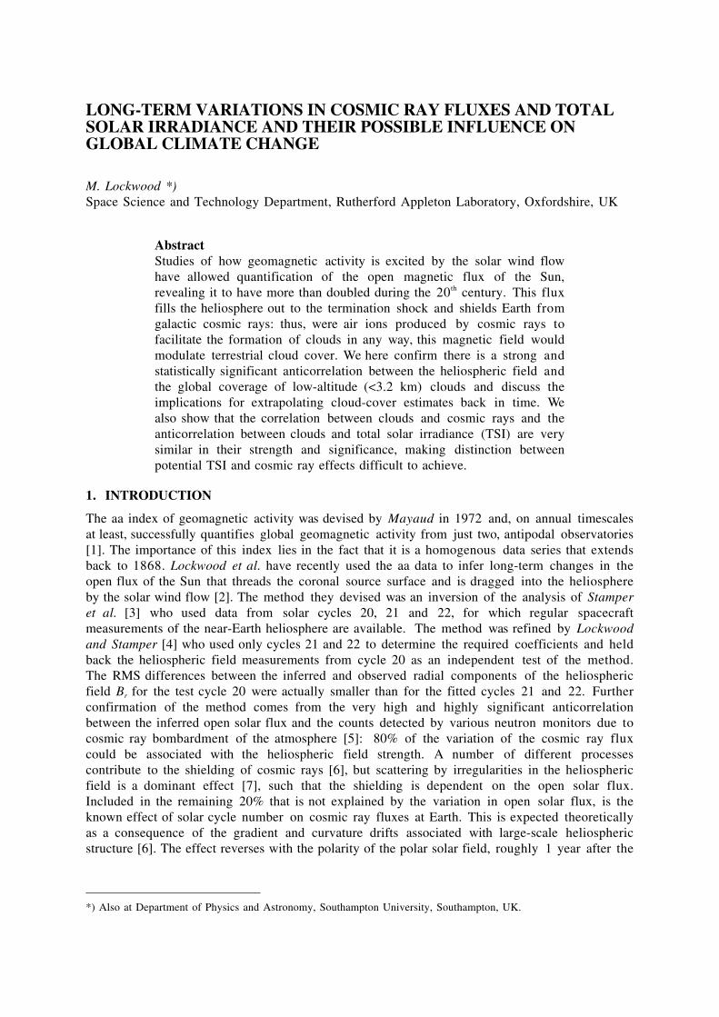
LONG-TERM VARIATIONS IN COSMIC RAY FLUXES AND TOTALSOLAR IRRADIANCE AND THEIR POSSIBLE INFLUENCE ONGLOBAL CLIMATE CHANGE

M. Lockwood *)Space Science and Technology Department, Rutherford Appleton Laboratory, Oxfordshire, UK

AbstractStudies of how geomagnetic activity is excited by the solar wind flowhave allowed quantification of the open magnetic flux of the Sun,revealing it to have more than doubled during the 20th century. This fluxfills the heliosphere out to the termination shock and shields Earth fromgalactic cosmic rays: thus, were air ions produced by cosmic rays tofacilitate the formation of clouds in any way, this magnetic field wouldmodulate terrestrial cloud cover. We here confirm there is a strong andstatistically significant anticorrelation between the heliospheric field andthe global coverage of low-altitude (<3.2 km) clouds and discuss theimplications for extrapolating cloud-cover estimates back in time. Wealso show that the correlation between clouds and cosmic rays and theanticorrelation between clouds and total solar irradiance (TSI) are verysimilar in their strength and significance, making distinction betweenpotential TSI and cosmic ray effects difficult to achieve.

1. INTRODUCTION

The aa index of geomagnetic activity was devised by Mayaud in 1972 and, on annual timescalesat least, successfully quantifies global geomagnetic activity from just two, antipodal observatories[1]. The importance of this index lies in the fact that it is a homogenous data series that extendsback to 1868. Lockwood et al. have recently used the aa data to infer long-term changes in theopen flux of the Sun that threads the coronal source surface and is dragged into the heliosphereby the solar wind flow [2]. The method they devised was an inversion of the analysis of Stamperet al. [3] who used data from solar cycles 20, 21 and 22, for which regular spacecraftmeasurements of the near-Earth heliosphere are available. The method was refined by Lockwoodand Stamper [4] who used only cycles 21 and 22 to determine the required coefficients and heldback the heliospheric field measurements from cycle 20 as an independent test of the method.The RMS differences between the inferred and observed radial components of the heliosphericfield Br for the test cycle 20 were actually smaller than for the fitted cycles 21 and 22. Furtherconfirmation of the method comes from the very high and highly significant anticorrelationbetween the inferred open solar flux and the counts detected by various neutron monitors due tocosmic ray bombardment of the atmosphere [5]: 80% of the variation of the cosmic ray fluxcould be associated with the heliospheric field strength. A number of different processescontribute to the shielding of cosmic rays [6], but scattering by irregularities in the heliosphericfield is a dominant effect [7], such that the shielding is dependent on the open solar flux.Included in the remaining 20% that is not explained by the variation in open solar flux, is theknown effect of solar cycle number on cosmic ray fluxes at Earth. This is expected theoreticallyas a consequence of the gradient and curvature drifts associated with large-scale heliosphericstructure [6]. The effect reverses with the polarity of the polar solar field, roughly 1 year after the

*) Also at Department of Physics and Astronomy, Southampton University, Southampton, UK.

peak of each cycle, and is apparent at the data, predominantly at solar minimum when theheliospheric field is weakest [7, 8, 9].

The method used to derive the heliospheric field is based on the theory of solar wind –magnetosphere coupling by Vasyluinas et al. [10], and thus by extrapolating back in time tobefore cycle 21 we are assuming that no there is no additional unknown factor, not included inthis theory, the behaviour of which is different on decadal and century timescales. Given thecorrelation obtained for cycles 21 and 22 is 0.97, to be relevant this factor would need to haveintroduced variability before the start of cycle 21, but not subsequently. An important point inthis respect is that the correlation between the open solar flux inferred from geomagnetic activityand cosmic ray neutron products was equally high and significant for solar cycles 19, 20, 21 and22. Thus the method has been confirmed by independent data from cycles 19 and 20 – despitethe fact that cycle 19 was the largest solar activity cycle ever observed and that cycle 20 wassurprisingly weak.

The key finding from the method is that the heliospheric field, averaged over full solarcycles, increased by 140% over the 20th century [2]. Extrapolating using the correlations with thecosmic ray fluxes discussed above, yields that the flux of primary cosmic rays was some 15%higher on average in 1900 than at present for energies above 3 GeV and 4% higher for >13GeV[5]. Support for this inferred drift comes from the abundance of the 10Be found, for example, inthe Dye-3 Greenland ice core [11, 12]. This is formed as a spallation product when cosmic raysimpact O and N in the atmosphere, and is then deposited in the ice sheet by precipitation. Thedependence of precipitation on climatic conditions introduces scatter, nevertheless a clearanticorrelation with the inferred open solar flux is found [5]. In addition, the variation of 14Cfound, for example, in tree rings is consistent with the change seen in 10Be [13]. The complicationfor both these isotopes is that the abundances detected are subject to climate change. However,the effect is very different in the two cases: 10Be is precipitated into ice sheets, a process thatintroduces lag and a dependence on climate, whereas 14C is directly absorbed in gaseous state buthas reservoirs in the biomass and oceans, exchange with which masks the true cosmogenicproduction rate and is expected to vary with climate. However, the similarity of the inferredcentury-scale changes in 10Be and 14C production rates strongly implies that the cause is a variationin cosmic rays and not climatic.

Svensmark and Friis-Christensen [14], Svensmark [15] and Marsh and Svensmark [16] havediscussed a correlation between cosmic ray fluxes and global cloud cover on Earth. Thecorrelation is best with higher energy cosmic ray fluxes and low-altitude cloud cover.

The present paper contains three studies. Given that the open solar flux quantifies 80% ofthe cosmic ray variation, section 2 looks at the direct correlation between open solar flux andcloud cover. We then use the long-term variation in the open flux derived from the aa index tolook at the possible change in global cloud cover since 1900, assuming the correlation were realand not influenced by any other factors. One possibility for such a factor is the total solarirradiance (TSI) of the Sun, which is now known to show a solar cycle variation [17, 18, 19] andwhich also shows an upward drift over the 20th century in a variety of reconstructions that employproxy data [4, 20, 21, 22]. The open solar flux, for the interval of the global cloud cover data atleast, is well correlated with the TSI [4, 23]. This correlation was originally found in annual meandata and before observations for the rising phase of solar cycle 23 became available [4]. However,recent work [23] has shown that the correlation, although somewhat lower in monthly averages(correlation coefficient, r = 0.61), is highly significant (>99.99%), and has been maintained insolar cycle 23. Section 3 compares the correlations between cosmic rays and cloud cover and TSIand cloud cover. Section 3 also considers the effect of temporal smoothing on the significance ofthese correlations.

2. CLOUD COVER AND OPEN SOLAR FLUX

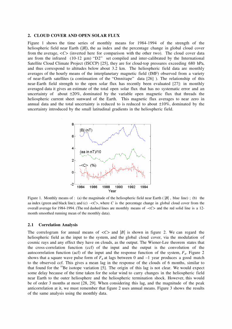
Figure 1 shows the time series of monthly means for 1984-1994 of the strength of theheliospheric field near Earth (|B|), the aa index and the percentage change in global cloud coverfrom the average, <C> (inverted here for comparison with the other two). The cloud cover dataare from the infrared (10-12 mm) “D2” set compiled and inter-calibrated by the InternationalSatellite Cloud Climate Project (ISCCP) [25], they are for cloud-top pressures exceeding 680 hPa,and thus correspond to altitudes below about 3.2 km. The heliospheric field data are monthlyaverages of the hourly means of the interplanetary magnetic field (IMF) observed from a varietyof near-Earth satellites (a continuation of the “Omnitape” data [26] ). The relationship of thisnear-Earth field strength to the open solar flux has recently been evaluated [27]: in monthlyaveraged data it gives an estimate of the total open solar flux that has no systematic error and anuncertainty of about ±20%, dominated by the variable open magnetic flux that threads theheliospheric current sheet sunward of the Earth. This magnetic flux averages to near zero inannual data and the total uncertainty is reduced to is reduced to about ±10%, dominated by theuncertainty introduced by the small latitudinal gradients in the heliospheric field.

Figure 1. Monthly means of : (a) the magnitude of the heliospheric field near Earth ( |B| , blue line) ; (b) theaa index (green and black line); and (c) -<C>, where C is the percentage change in global cloud cover from theoverall average for 1984-1994. (The red dashed lines are monthly means of -<C> and the red solid line is a 12-month smoothed running mean of the monthly data).

2.1 Correlation Analysis

The correlogram for annual means of <C> and |B | is shown in figure 2. We can regard theheliospheric field as the input to the system, and the global cloud cover, via the modulation ofcosmic rays and any effect they have on clouds, as the output. The Wiener-Lee theorem states thatthe cross-correlation function (ccf) of the input and the output is the convolution of theautocorrelation function (acf) of the input and the response function of the system, FR. Figure 2shows that a square wave pulse form of FR at lags between 0 and –1 year produces a good matchto the observed ccf. This gives a mean lag in the response of the clouds of 6 months, similar tothat found for the 10Be isotope variation [5]. The origin of this lag is not clear. We would expectsome delay because of the time taken for the solar wind to carry changes in the heliospheric fieldnear Earth to the outer heliosphere and the heliospheric termination shock. However, this wouldbe of order 3 months at most [28, 29]. When considering this lag, and the magnitude of the peakanticorrelation at it, we must remember that figure 2 uses annual means. Figure 3 shows the resultsof the same analysis using the monthly data.

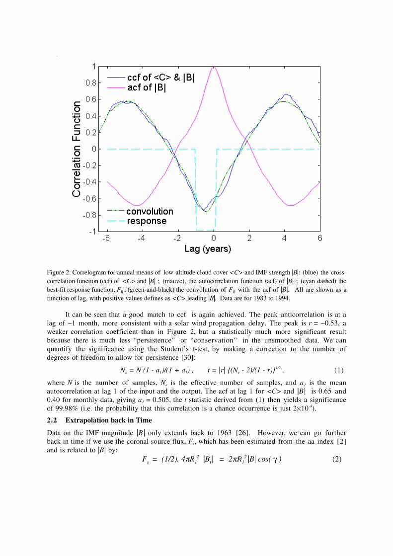
Figure 2. Correlogram for annual means of low-altitude cloud cover <C> and IMF strength |B|: (blue) the cross-correlation function (ccf) of <C> and |B| ; (mauve), the autocorrelation function (acf) of |B| ; (cyan dashed) thebest-fit response function, FR ; (green-and-black) the convolution of FR with the acf of |B|. All are shown as afunction of lag, with positive values defines as <C> leading |B|. Data are for 1983 to 1994.

It can be seen that a good match to ccf is again achieved. The peak anticorrelation is at alag of –1 month, more consistent with a solar wind propagation delay. The peak is r = –0.53, aweaker correlation coefficient than in Figure 2, but a statistically much more significant resultbecause there is much less “persistence” or “conservation” in the unsmoothed data. We canquantify the significance using the Student’s t-test, by making a correction to the number ofdegrees of freedom to allow for persistence [30]:

Ne = N (1 - a1)/(1 + a1) , t = |r| (Ne - 2)/(1 - r)1/2 , (1)

where N is the number of samples, Ne is the effective number of samples, and a1 is the meanautocorrelation at lag 1 of the input and the output. The acf at lag 1 for <C> and |B | is 0.65 and0.40 for monthly data, giving a1 = 0.505, the t statistic derived from (1) then yields a significanceof 99.98% (i.e. the probability that this correlation is a chance occurrence is just 2¥10-4).

2.2 Extrapolation back in Time

Data on the IMF magnitude |B | only extends back to 1963 [26]. However, we can go furtherback in time if we use the coronal source flux, Fs, which has been estimated from the aa index [2]and is related to |B| by:

Fs = (1/2). 4pR12 |Br| = 2pR1

2 |B| cos( g ) (2)

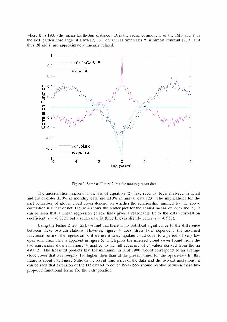
where R1 is 1AU (the mean Earth-Sun distance), Br is the radial component of the IMF and g isthe IMF garden hose angle at Earth [2, 23]: on annual timescales g is almost constant [2, 3] andthus |B| and Fs are approximately linearly related.

Figure 3. Same as Figure 2, but for monthly mean data

The uncertainties inherent in the use of equation (2) have recently been analysed in detailand are of order ±20% in monthly data and ±10% in annual data [23]. The implications for thepast behaviour of global cloud cover depend on whether the relationship implied by the abovecorrelation is linear or not. Figure 4 shows the scatter plot for the annual means of <C> and Fs. Itcan be seen that a linear regression (black line) gives a reasonable fit to the data (correlationcoefficient, r = -0.932), but a square-law fit (blue line) is slightly better (r = -0.957).

Using the Fisher-Z test [23], we find that there is no statistical significance to the differencebetween these two correlations. However, figure 4 does stress how dependent the assumedfunctional form of the regression is, if we use it to extrapolate cloud cover to a period of very lowopen solar flux. This is apparent in figure 5, which plots the inferred cloud cover found from thetwo regressions shown in figure 4, applied to the full sequence of Fs values derived from the aadata [2]. The linear fit predicts that the minimum in Fs at 1900 would correspond to an averagecloud cover that was roughly 1% higher then than at the present time: for the square-law fit, thisfigure is about 3%. Figure 5 shows the recent time series of the data and the two extrapolations: itcan be seen that extension of the D2 dataset to cover 1994-1999 should resolve between these twoproposed functional forms for the extrapolation.

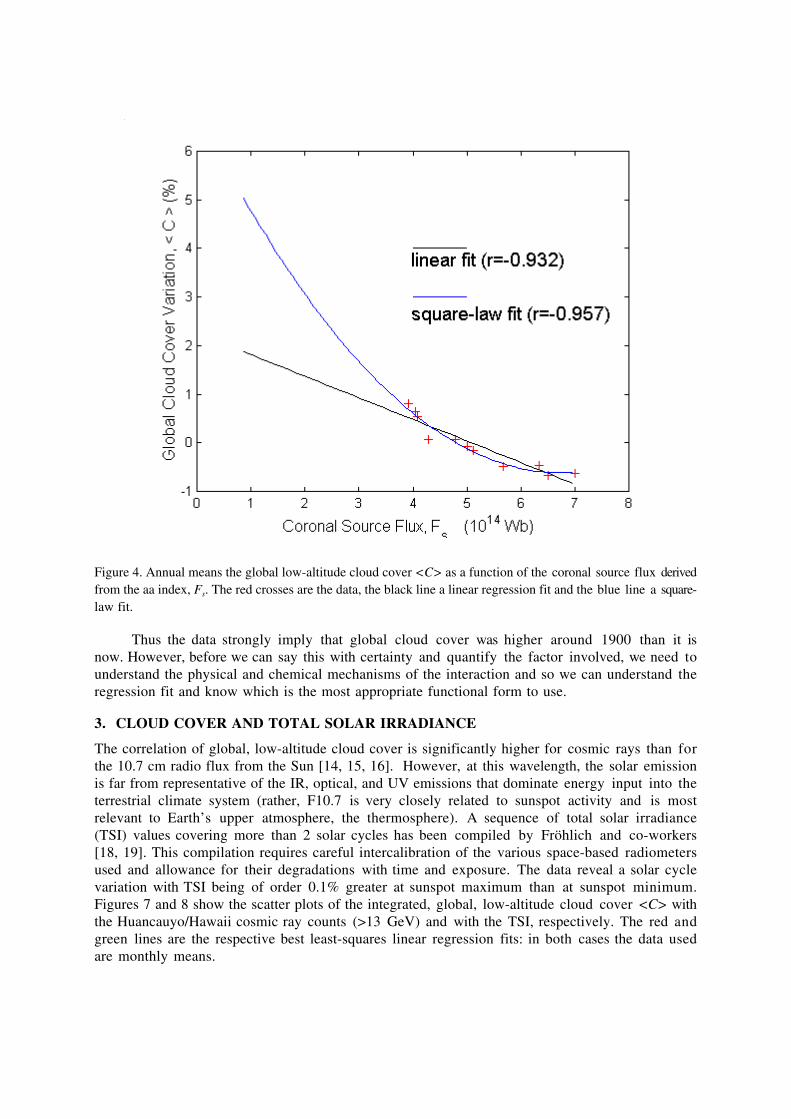
Figure 4. Annual means the global low-altitude cloud cover <C> as a function of the coronal source flux derivedfrom the aa index, Fs. The red crosses are the data, the black line a linear regression fit and the blue line a square-law fit.

Thus the data strongly imply that global cloud cover was higher around 1900 than it isnow. However, before we can say this with certainty and quantify the factor involved, we need tounderstand the physical and chemical mechanisms of the interaction and so we can understand theregression fit and know which is the most appropriate functional form to use.

3. CLOUD COVER AND TOTAL SOLAR IRRADIANCE

The correlation of global, low-altitude cloud cover is significantly higher for cosmic rays than forthe 10.7 cm radio flux from the Sun [14, 15, 16]. However, at this wavelength, the solar emissionis far from representative of the IR, optical, and UV emissions that dominate energy input into theterrestrial climate system (rather, F10.7 is very closely related to sunspot activity and is mostrelevant to Earth’s upper atmosphere, the thermosphere). A sequence of total solar irradiance(TSI) values covering more than 2 solar cycles has been compiled by Fröhlich and co-workers[18, 19]. This compilation requires careful intercalibration of the various space-based radiometersused and allowance for their degradations with time and exposure. The data reveal a solar cyclevariation with TSI being of order 0.1% greater at sunspot maximum than at sunspot minimum.Figures 7 and 8 show the scatter plots of the integrated, global, low-altitude cloud cover <C> withthe Huancauyo/Hawaii cosmic ray counts (>13 GeV) and with the TSI, respectively. The red andgreen lines are the respective best least-squares linear regression fits: in both cases the data usedare monthly means.

The peak correlation coefficients for the data shown in figures 7 and 8 were both obtainedfor zero lag between the data series and were -0.741 and +0.654 (for TSI and cosmic rays,respectively). Using the Students t-test discussed above, these correlations are significant at the99.8% and 99.6% levels. Although the correlation is marginally higher for TSI than for thecosmic rays, the Fisher-Z test [23] tells us that the difference between these two correlations is notsignificant (the significance level being only 30.1%, i.e. the probability that the difference aroseby chance is 0.699).

Figure 5. Extrapolated low-altitude global cloud cover estimates for 1868-1998: (black) from a linear fit toobservation; and (blue) from a square-law loss. The observed data are shown in red.

Figure 6. Detail from Figure 5 for 1980-2000.

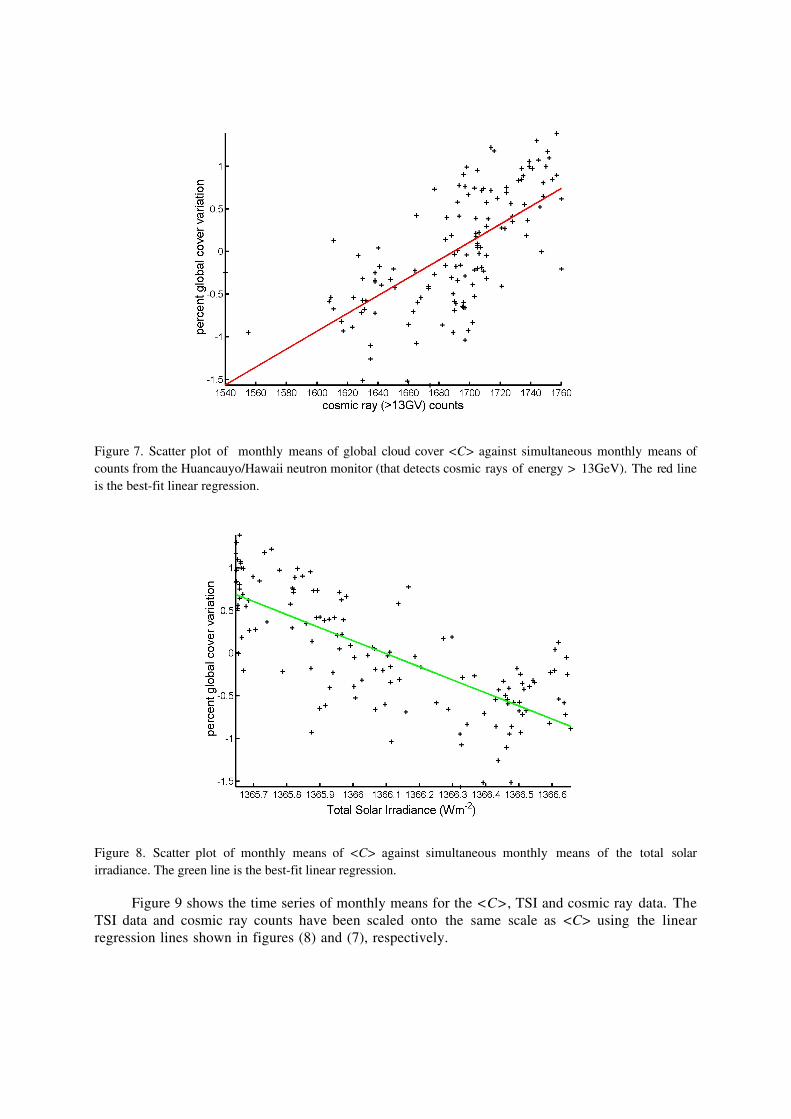
Figure 7. Scatter plot of monthly means of global cloud cover <C> against simultaneous monthly means ofcounts from the Huancauyo/Hawaii neutron monitor (that detects cosmic rays of energy > 13GeV). The red lineis the best-fit linear regression.

Figure 8. Scatter plot of monthly means of <C> against simultaneous monthly means of the total solarirradiance. The green line is the best-fit linear regression.

Figure 9 shows the time series of monthly means for the <C>, TSI and cosmic ray data. TheTSI data and cosmic ray counts have been scaled onto the same scale as <C> using the linearregression lines shown in figures (8) and (7), respectively.

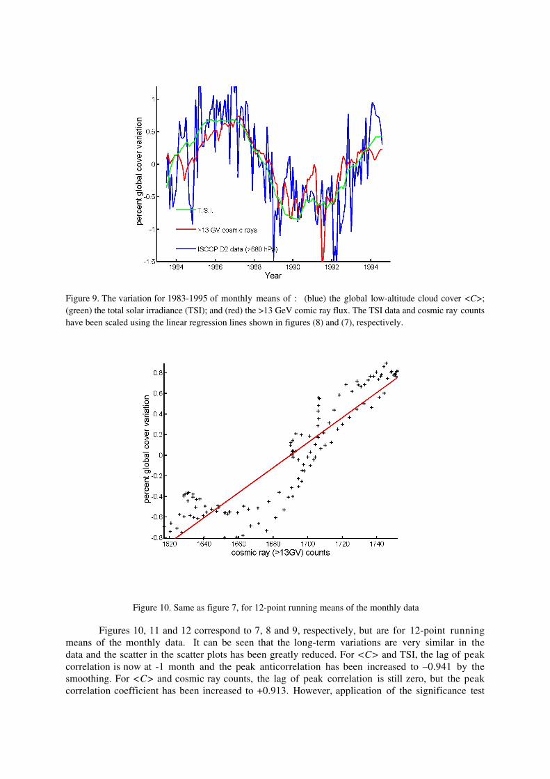
Figure 9. The variation for 1983-1995 of monthly means of : (blue) the global low-altitude cloud cover <C>;(green) the total solar irradiance (TSI); and (red) the >13 GeV comic ray flux. The TSI data and cosmic ray countshave been scaled using the linear regression lines shown in figures (8) and (7), respectively.

Figure 10. Same as figure 7, for 12-point running means of the monthly data

Figures 10, 11 and 12 correspond to 7, 8 and 9, respectively, but are for 12-point runningmeans of the monthly data. It can be seen that the long-term variations are very similar in thedata and the scatter in the scatter plots has been greatly reduced. For <C> and TSI, the lag of peakcorrelation is now at -1 month and the peak anticorrelation has been increased to –0.941 by thesmoothing. For <C> and cosmic ray counts, the lag of peak correlation is still zero, but the peakcorrelation coefficient has been increased to +0.913. However, application of the significance test

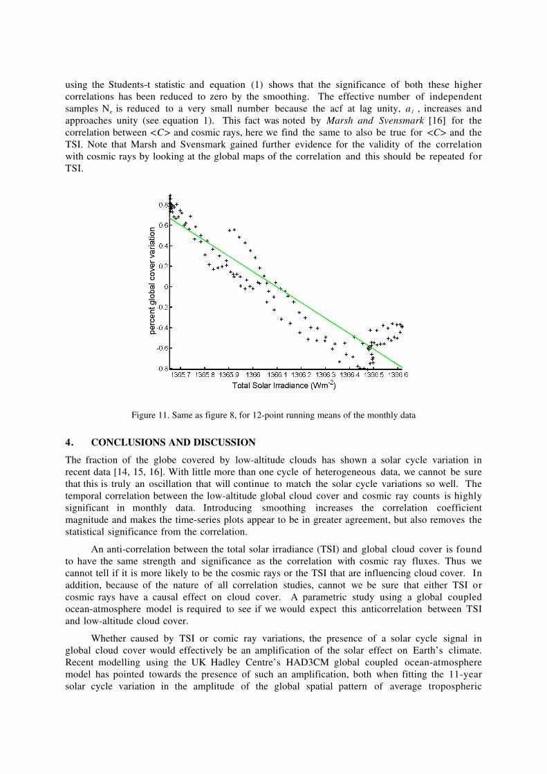
using the Students-t statistic and equation (1) shows that the significance of both these highercorrelations has been reduced to zero by the smoothing. The effective number of independentsamples Ne is reduced to a very small number because the acf at lag unity, a1 , increases andapproaches unity (see equation 1). This fact was noted by Marsh and Svensmark [16] for thecorrelation between <C> and cosmic rays, here we find the same to also be true for <C> and theTSI. Note that Marsh and Svensmark gained further evidence for the validity of the correlationwith cosmic rays by looking at the global maps of the correlation and this should be repeated forTSI.

Figure 11. Same as figure 8, for 12-point running means of the monthly data

4. CONCLUSIONS AND DISCUSSION

The fraction of the globe covered by low-altitude clouds has shown a solar cycle variation inrecent data [14, 15, 16]. With little more than one cycle of heterogeneous data, we cannot be surethat this is truly an oscillation that will continue to match the solar cycle variations so well. Thetemporal correlation between the low-altitude global cloud cover and cosmic ray counts is highlysignificant in monthly data. Introducing smoothing increases the correlation coefficientmagnitude and makes the time-series plots appear to be in greater agreement, but also removes thestatistical significance from the correlation.

An anti-correlation between the total solar irradiance (TSI) and global cloud cover is foundto have the same strength and significance as the correlation with cosmic ray fluxes. Thus wecannot tell if it is more likely to be the cosmic rays or the TSI that are influencing cloud cover. Inaddition, because of the nature of all correlation studies, cannot we be sure that either TSI orcosmic rays have a causal effect on cloud cover. A parametric study using a global coupledocean-atmosphere model is required to see if we would expect this anticorrelation between TSIand low-altitude cloud cover.

Whether caused by TSI or comic ray variations, the presence of a solar cycle signal inglobal cloud cover would effectively be an amplification of the solar effect on Earth’s climate.Recent modelling using the UK Hadley Centre’s HAD3CM global coupled ocean-atmospheremodel has pointed towards the presence of such an amplification, both when fitting the 11-yearsolar cycle variation in the amplitude of the global spatial pattern of average tropospheric

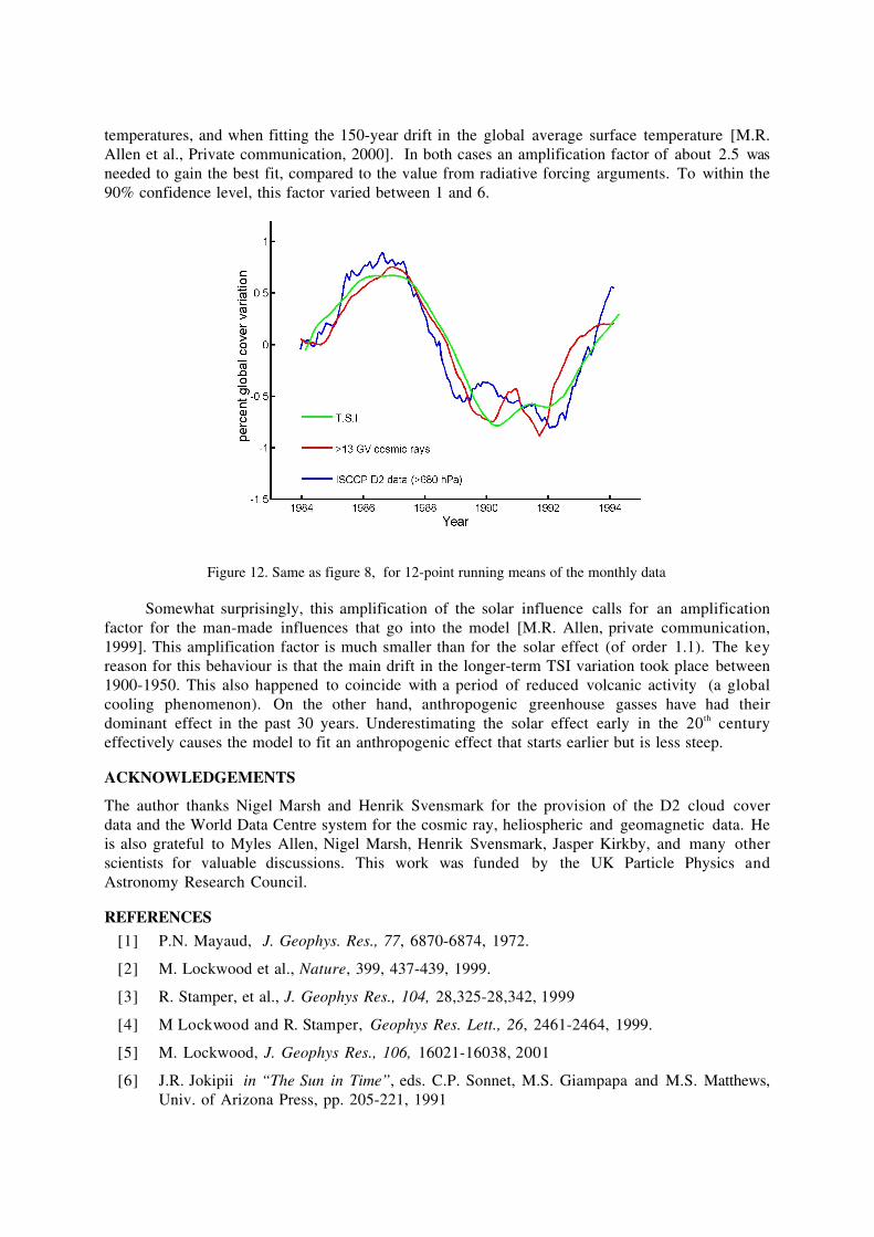
temperatures, and when fitting the 150-year drift in the global average surface temperature [M.R.Allen et al., Private communication, 2000]. In both cases an amplification factor of about 2.5 wasneeded to gain the best fit, compared to the value from radiative forcing arguments. To within the90% confidence level, this factor varied between 1 and 6.

Figure 12. Same as figure 8, for 12-point running means of the monthly data

Somewhat surprisingly, this amplification of the solar influence calls for an amplificationfactor for the man-made influences that go into the model [M.R. Allen, private communication,1999]. This amplification factor is much smaller than for the solar effect (of order 1.1). The keyreason for this behaviour is that the main drift in the longer-term TSI variation took place between1900-1950. This also happened to coincide with a period of reduced volcanic activity (a globalcooling phenomenon). On the other hand, anthropogenic greenhouse gasses have had theirdominant effect in the past 30 years. Underestimating the solar effect early in the 20th centuryeffectively causes the model to fit an anthropogenic effect that starts earlier but is less steep.

ACKNOWLEDGEMENTS

The author thanks Nigel Marsh and Henrik Svensmark for the provision of the D2 cloud coverdata and the World Data Centre system for the cosmic ray, heliospheric and geomagnetic data. Heis also grateful to Myles Allen, Nigel Marsh, Henrik Svensmark, Jasper Kirkby, and many otherscientists for valuable discussions. This work was funded by the UK Particle Physics andAstronomy Research Council.

REFERENCES

[1] P.N. Mayaud, J. Geophys. Res., 77, 6870-6874, 1972.

[2] M. Lockwood et al., Nature, 399, 437-439, 1999.

[3] R. Stamper, et al., J. Geophys Res., 104, 28,325-28,342, 1999

[4] M Lockwood and R. Stamper, Geophys Res. Lett., 26, 2461-2464, 1999.

[5] M. Lockwood, J. Geophys Res., 106, 16021-16038, 2001

[6] J.R. Jokipii in “The Sun in Time”, eds. C.P. Sonnet, M.S. Giampapa and M.S. Matthews, Univ. of Arizona Press, pp. 205-221, 1991

[7] H.V. Cane, Geophys. Res. Lett., 26, 565-568, 1999

[8] I.G. Usoskin, J. Geophys.Res., 103, 9567-9574, 1998.

[9] H.S. Ahluwalia, J. Geophys. Res., 102, 24,229-24,236, 1997

[10] V.M. Vasyliunas, Planet Space Sci., 30, 359-365, 1982.

[11] K.G. McCracken and F.B. McDonald, The long-term modulation of the galactic cosmicradiation, 1500-2000, in press, in Proc. 27th. Int. Cosmic Ray Conference, Hamburg, 2001

[12] J. Beer et al., Sol. Phys., 181, 237-249, 1998.

[13] E. Bard, et al., Earth and Planet. Sci. Lett., 150, 453-462, 1997.

[14] H. Svensmark, and E. Friis-Christensen, J. Atmos. Sol. Terr. Phys., 59, 1225-1232, 1997.

[15] H. Svensmark, Phys. Rev. Lett., 81, 5027-5030, 1998.

[16] N. Marsh, and H. Svensmark, Space Sci. Rev., 94, (1/2), 215-230, 2000.

[17] R.C. Willson, Science, 277, 1963-1965, 1997.

[18] C. Fröhlich, and J. Lean, Geophys. Res. Lett., 25, 4377-4380, 1998.

[19] C. Fröhlich, Space Sci. Rev., 94, (1/2), 15-24, 2000.

[20] J. Lean, et al., Geophys. Res. Lett., 22, 3195-3198, 1995.

[21] S.K. Solanki and M. Fligge, Geophys. Res. Lett., 26, 2465-2468, 1999.

[22] Hoyt, D., and K. Schatten, J. Geophys. Res., 98, 18,895-18,906, 1993.

[23] M. Lockwood, An evaluation of the correlation between open solar flux and total solarirradiance, Astron and Astrophys., in press, 2001.

[24] Y.-M. Wang, Geophys. Res. Lett., 27, 621-624, 2000.

[25] W.B. Rossow, et al., International Satellite Cloud Climatology Project (ISCCP):Documentation of new datasets, WMO/TD 737, World Meteorol. Organ., Geneva, 1996.

[26] D. A. Couzens and J. H. King, Interplanetary Medium Data Book - Supplement 3, NationalSpace Science Data Center, Goddard Space Flight Center, Greenbelt, Maryland, USA, 1986.

[27] M. Lockwood, The relationship between the near-Earth Interplanetary field and thecoronal source flux: dependence on timescale, J. Geophys. Res., in press, 2001.

[28] M.S. Potgieter, Adv. in Space Res, 16(9), 191-203, 1995.

[29] A.C. Cummings et al., J. Geophys. Res., 99, 11,547-11,552, 1994.

[30] Wilks, D.S., Statistical methods in the atmospheric sciences, Academic Press, San Diego,California, USA, 1995.

EVIDENCE FROM THE PAST: SOLAR FORCING OF CLIMATECHANGE BY WAY OF COSMIC RAYS AND/OR BY SOLAR UV?

Bas van Geel1, Hans Renssen2 and Johannes van der Plicht3

1 Institute for Biodiversity and Ecosystem Dynamics, Universiteit van Amsterdam, Kruislaan 318,1098 SM Amsterdam, The Netherlands vangeel@science.uva.nl2 Institut d´Astronomie et de Géophysique G. Lemaître, Université Catholique de Louvain, 2Chemin du Cyclotron, B-1348 Louvain-la-Neuve, Belgium renssen@astr.ucl.ac.be3 Centre for Isotope Research, University of Groningen, Nijenborgh 4, 9747 AG Groningen, TheNetherlands plicht@phys.rug.nl

AbstractMajor Holocene shifts to cool and wet climate types in the temperatezones correspond to suddenly increasing values of the atmospheric 14Ccontent, suggesting a link between changing solar activity and climatechange. In the temperate zones the transition from the Subboreal to theSubatlantic (ca 850 cal BC) represents a sudden, strong shift from arelatively dry and warm climate to a humid and cool episode. Themoment of change occurred at, or maybe even just before the start of asharp rise of the atmospheric 14C content. In previous studies, wepostulated two amplification mechanisms: a) increased cosmic ray fluxcauses an increase in atmospheric 14C content, and also a climate shift, b)a decline of solar UV causes a reduced stratospheric ozone concentration,leading to climate change at the earth surface. Two phenomena indicatethat mechanism a) is much less likely than mechanism b):1) The enhancement of cosmic ray intensity to relatively high levels tookplace several decades after the climate shift.2) In Central Africa and in Western India there was a shift to dryness.Chronological differentiation in solar output may play a role, but this ispurely hypothetical.

1. INTRODUCTION

Over the last few hundred years, changes in solar irradiance have been relatively small (less than 1W/m2). As a consequence, solar forcing of abrupt climate change has been controversial [1].However, there is strong evidence from the past for an important role of the sun upon climatechange [2-5]. To explain this past evidence of solar forcing, we postulated two possibleamplifying mechanisms that could explain how relatively small changes in solar irradiance couldlead to abrupt climatic shifts [6].

a) Changes of cosmic ray intensity (modulated by fluctuating solar wind) might have an effect oncloud formation and thus on the planetary albedo and on temperature [7], and/or

b) Within the small changes of solar activity, changes in UV are important [1]. Changes in solarUV have an effect on ozone formation in the lower stratosphere. Variations in the ozoneconcentration modulate the stratospheric temperature, leading to changes in the stratosphericcirculation that could be propagated downwards to the Earth’s surface, thus influencingatmospheric circulation patterns world-wide [8, 9].

We review the evidence for solar forcing of climate change at the Subboreal-Subatlantictransition, as found in raised bogs and other paleodata, and we evaluate the possible contributionof both mechanisms mentioned above.

2. RAISED BOG AS ARCHIVES OF PAST CLIMATE

Peat deposits are valuable archives for paleoclimate studies. The so-called raised bogs in NW-Europe are rainwater fed and the paleohydrological changes of such bogs mainly reflect climateshifts. A climate shift around 850 calendar years BC is visible in raised bog profiles as a transitionfrom peat which was formed during a period of a relatively warm climate (darker, moredecomposed peat) to lighter coloured upper peat, formed during a period of cooler, wetterclimatic conditions. We use the Radiocarbon (14C) method for precise dating of climate-inducedtransitions in peat layers. Radiocarbon ages are expressed in BP, Radiocarbon "years" relative to1950 AD. Radiocarbon years are different from calendar years because the production of 14C hasnot been constant in the past due to changes in both the geomagnetic field strength and in solaractivity. The 14C time scale is calibrated by measuring the 14C content of tree rings, datedabsolutely by means of dendrochronology [10]. The solar activity changes characterise thecalibration curve by means of fluctuations (the so-called "wiggles"). Calibration of a singleRadiocarbon date usually yields an irregular probability distribution in calendar age, quite oftenover a long time interval. This is problematic in paleoclimatological studies, especially when aprecise temporal comparison between different climate proxies is required. However, a sequenceof (uncalibrated) 14C dates can be matched to the wiggles in the calibration curve (wiggle-matchdating [11, 12]). A high-resolution 14C sample sequence can result in a precise chronology of thepeat core. This dating strategy also revealed relationships between atmospheric 14C variations andshort-term climatic fluctuations (as detected in peat deposits) caused by solar variations. Data fromHolocene lake deposits in the Jura Mountains also strongly point to a relationship between 14Cfluctuations and paleohydrological shifts under the influence of climate change [2].

The climate shift around 850 cal BC (Subboreal-Subatlantic transition) was one of the mostimportant climate shifts during the Holocene. We focused on this transition, which wasimmediately followed by a sharp rise of the atmospheric 14C content during the period between850 and 760 cal BC. We identified the peat-forming mosses (representatives of the genusSphagnum) in peat profiles of Northwest and Central European raised bogs. Knowing theecological preferences of the mosses, we could interpret the recorded changes in speciescomposition in terms of hydrological changes, related to climate change [13, 14]. Before theclimate shift from the Subboreal to the Subatlantic period, Sphagna of the section Acutifolia wereimportant peat formers in the Dutch bogs. Then Sphagnum papillosum and Sphagnumimbricatum took over. This change of the peat-forming plants indicates a shift from relativelywarm, to cooler, wetter climatic conditions. The paleo-record from raised bogs shows that theabrupt climate shift happened at, or maybe even shortly before, the start of the period of thesharply rising atmospheric 14C content (Figure 1). In various lowland regions in the Netherlandswhere settlement sites were present, the climate shift at the Subboreal-Subatlantic transition causeda considerable rise of the ground water table so that arable land was transformed into wetland,where peat growth started. Bronze Age farmers living in such areas had to migrate because theycould no longer produce enough food in their original settlement areas. Like the raised bogevidence, the archaeological evidence also points to a climate shift just preceding the enhancedcosmic ray intensity [13].

We also found strong evidence for climate change around 850 cal BC in other parts of theworld [15, 16 and references therein]. In the temperate zones of Europe, North America andSouth America there is evidence for an equatorward shift of suddenly enhanced Westerlies, whilethe climate changed (cooling, higher effective precipitation).

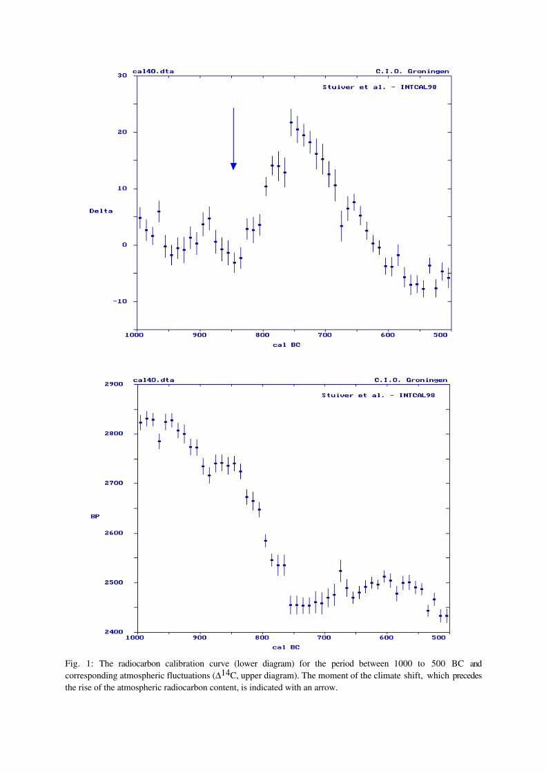
Fig. 1: The radiocarbon calibration curve (lower diagram) for the period between 1000 to 500 BC andcorresponding atmospheric fluctuations (D14C, upper diagram). The moment of the climate shift, which precedesthe rise of the atmospheric radiocarbon content, is indicated with an arrow.

3. THE CONTRIBUTION OF AMPLIFYING MECHANISMS

The observed climate changes around 850 cal BC may have been caused by the lowering of solarirradiation through two amplifying factors, namely, (1) increased cosmic ray intensity stimulating

polar front

0°

30°N

60°N

30°S

60°S

HadleyCell

Ferrel Cell

Polar Cell

PrevailingWesterlies

N.E. Trades

S.E. Trades

ITCZ

PrevailingWesterlies

Polar Easterlies

Polar Easterlies

PFJ

PFJ

STJ

STJ

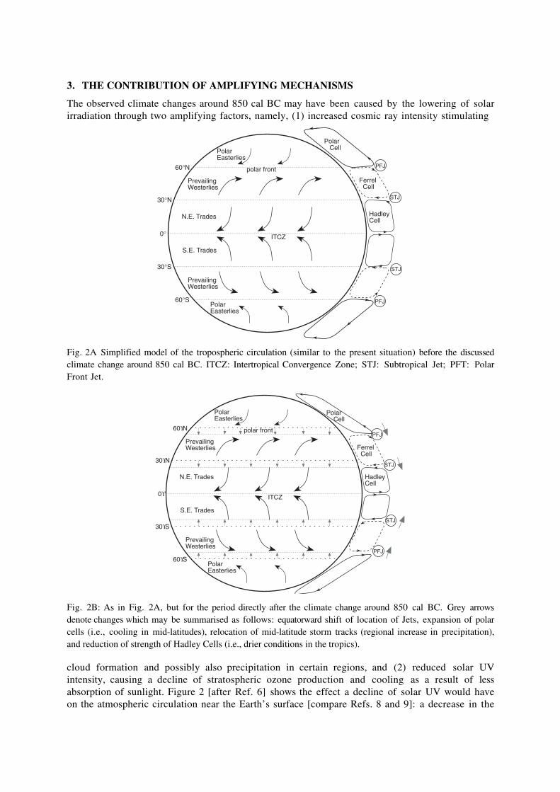
Fig. 2A Simplified model of the tropospheric circulation (similar to the present situation) before the discussedclimate change around 850 cal BC. ITCZ: Intertropical Convergence Zone; STJ: Subtropical Jet; PFT: PolarFront Jet.

polar front

0°

30°N

60°N

30°S

60°S

HadleyCell

Ferrel Cell

Polar Cell

PrevailingWesterlies

N.E. Trades

S.E. Trades

ITCZ

PrevailingWesterlies

Polar Easterlies

Polar Easterlies

PFJ

PFJ

STJ

STJ

Fig. 2B: As in Fig. 2A, but for the period directly after the climate change around 850 cal BC. Grey arrowsdenote changes which may be summarised as follows: equatorward shift of location of Jets, expansion of polarcells (i.e., cooling in mid-latitudes), relocation of mid-latitude storm tracks (regional increase in precipitation),and reduction of strength of Hadley Cells (i.e., drier conditions in the tropics).

cloud formation and possibly also precipitation in certain regions, and (2) reduced solar UVintensity, causing a decline of stratospheric ozone production and cooling as a result of lessabsorption of sunlight. Figure 2 [after Ref. 6] shows the effect a decline of solar UV would haveon the atmospheric circulation near the Earth’s surface [compare Refs. 8 and 9]: a decrease in the

latitudinal extent of Hadley Cell circulation (weakening of the monsoon) may have occurred withconcomitant equatorward relocation of mid-latitude storm tracks [see also Ref. 17]. This picturefits in with the paleoclimatological evidence from the northern and southern temperate zones(cooler, wetter) and the contemporaneous dryness crisis in Central Africa and Western India, whichis evident from pollen records and archaeological evidence [13, 16]. The evidence during theSubboreal-Subatlantic transition strongly supports the "Haigh model" [8, 9] as an effectiveamplification mechanism for changes in solar activity. The combination of detailedpaleoclimatological data from different parts of the world delivers circumstantial evidence for thesuggestion that the UV-ozone mechanism had more effect on climate than the mechanism relatedto the increase of the cosmic ray intensity.

In summary, we conclude that there is paleo-evidence for solar forcing of climate changearound 850 cal BC. Of the two possible amplification mechanisms, the reduced UV scenario wasmost likely the effective one. There seem to be two arguments against an important role of cosmicrays (cloud formation) in relation to climate change:

1) Detailed series of radiocarbon dates from archaeological sites and raised bogs [11, 13, 14, 18]show that the abrupt climate change around 850 cal BC had already occurred when thecosmogenic isotope 14C only started to show an initially insignificant rise. This is supported bydata for 10Be (another cosmogenic isotope, the production of which more directly reflectschanging cosmic ray intensities than 14C), showing a corresponding and more or lesscontemporaneous rise as shown by 14C. For this event there might be a delay of approximately10 years in the 14C rise only [J. Beer, pers. comm.; compare Ref. 19]. Consequently, the time-lag in the rise of the 14C content (compared to climate change) cannot be attributed to possibledelaying processes related to the carbon cycle. In other words: the strong rise in cosmic rayintensity only followed climate change, and thus cannot have triggered the change [compareRef. 12 for major climate shifts during the Little Ice Age in relation to similar increases ofatmospheric Radiocarbon].

2) The widespread dryness in the tropics (weaker monsoon in Central Africa and Western India)after 850 cal BC is not an effect that is expected to occur with enhanced cloud formation underthe influence of increased cosmic ray intensity. However, the dryness in the tropics may not beinconsistent, as climatic teleconnections are not always straightforward (e.g., in the case of ElNiño) and it could be that cooling in the mid-latitudes (where enhanced cloud formation dueto increased cosmic ray intensities may be favoured) has resulted in drying in some regions inthe tropics. On the other hand, it must be noted that the observed world-wide, but stronglycontrasting changes in climate at the Subboreal-Subatlantic transition fit remarkably well in themodel for an important role of solar UV (see Fig. 2).

An important role for the reduced UV-scenario would raise one, yet unanswered, question:could a considerable decline of solar activity indeed have chronologically different phases(effective electromagnetic signal before magnetic signal; so first a UV decline with strong effectson climate, and later a more gradual decline of solar wind affecting the increased production ofcosmogenic isotopes)? Solar physicists might be able to answer this question. Alternatively,detailed observations of variations in solar activity in the near future may reveal a solution to thequestion about which amplification mechanism plays a role in solar forcing of climate change.

ACKNOWLEDGEMENTS

We thank Jürg Beer and Raimund Muscheler for critical reading of the manuscript and DmitriMauquoy for correction of the text.

REFERENCES

[1] D.V. Hoyt and K.H. Schatten, The role of the sun in climate change, Oxford, 1997(Oxford University Press)

[2] M. Magny, Quat. Res. 40 (1993) 1.

[3] B. van Geel et al., Quat. Sc. Rev. 18 (1999) 331.

[4] D.A. Hodell et al., Science 292 (2001) 1367.

[5] U. Neff et al., Nature 411 (2001) 291.

[6] B. van Geel and H. Renssen, In: Water, Environment and Society in Times of ClimaticChange (Kluwer, Dordrecht, 1998) p. 21-41.

[7] H. Svensmark and E. Friis-Christensen, J. Atm. Sol. Terr. Phys. 59 (1997) 1225.

[8] J.D. Haigh, Nature 370 (1994) 544.

[9] J.D. Haigh, Science 272 (1996) 981.

[10] M. Stuiver et al., Radiocarbon 40 (1998) 1041.

[11] M.R. Kilian et al., , 2000. Quat. Sc. Rev. 19 (2000) 1011.

[12] D. Mauquoy et al., Evidence from North-West European bogs showing that Little Ice Ageclimatic changes were driven by changes in solar activity. Holocene 12: in press.

[13] B. van Geel et al., Radiocarbon 40 (1998) 535.

[14] A. Speranza et al., Quat. Sc. Rev. 19 (2000) 1589.

[15] B. van Geel et al., 2000. Holocene 10 (2000) 659.

[16] B. van Geel et al., 2001. In: Y. Yasuda and V. Shinde (Eds), Monsoon and Civilization,Extended Abstracts of the 2nd International Workshop of the Asian Lake DrillingProgramme (Pune, India, 2001) p. 35.

[17] D. Shindell et al., Science 284 (1999) 305.

[18] B. van Geel et al., J. Quat. Sc. 11 (1996) 451.

[19] R. Muscheler et al., Terra Nostra 3 (2001) 156.

THE ROLE OF CLOUD COVER VARIATIONS ON THE SOLARILLUMINATION SIGNAL RECORDED BY dddd13C OF A SHALLOWWATER IONIAN SEA CORE (1147-1975 AD)

G.Cini Castagnoli, G. Bonino, D.Cane and C.TariccoDipartimento di Fisica Generale dell'Università, Via P.Giuria 1, 10125 Torino, and Istituto diCosmogeofisica del CNR, Corso Fiume 4, 10133 Torino, Italy

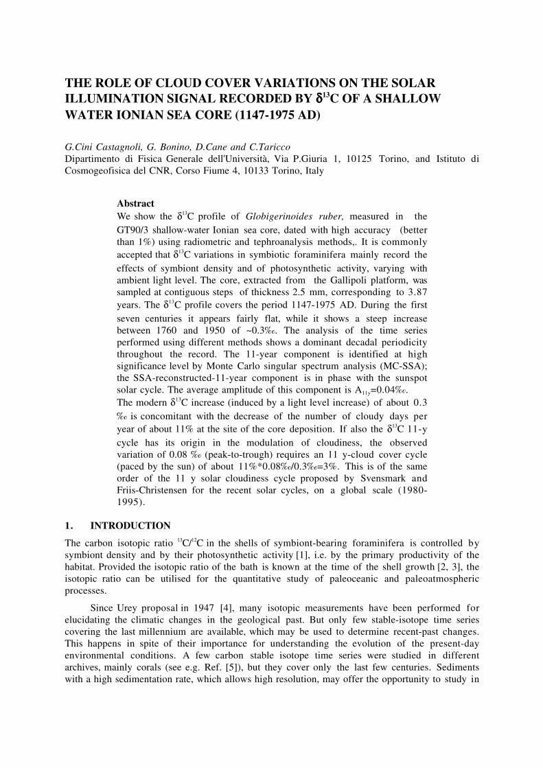
AbstractWe show the d13C profile of Globigerinoides ruber, measured in theGT90/3 shallow-water Ionian sea core, dated with high accuracy (betterthan 1%) using radiometric and tephroanalysis methods,. It is commonlyaccepted that d13C variations in symbiotic foraminifera mainly record theeffects of symbiont density and of photosynthetic activity, varying withambient light level. The core, extracted from the Gallipoli platform, wassampled at contiguous steps of thickness 2.5 mm, corresponding to 3.87years. The d13C profile covers the period 1147-1975 AD. During the firstseven centuries it appears fairly flat, while it shows a steep increasebetween 1760 and 1950 of ~0.3‰. The analysis of the time seriesperformed using different methods shows a dominant decadal periodicitythroughout the record. The 11-year component is identified at highsignificance level by Monte Carlo singular spectrum analysis (MC-SSA);the SSA-reconstructed-11-year component is in phase with the sunspotsolar cycle. The average amplitude of this component is A11y=0.04‰.The modern d13C increase (induced by a light level increase) of about 0.3‰ is concomitant with the decrease of the number of cloudy days peryear of about 11% at the site of the core deposition. If also the d13C 11-ycycle has its origin in the modulation of cloudiness, the observedvariation of 0.08 ‰ (peak-to-trough) requires an 11 y-cloud cover cycle(paced by the sun) of about 11%*0.08‰/0.3‰=3%. This is of the sameorder of the 11 y solar cloudiness cycle proposed by Svensmark andFriis-Christensen for the recent solar cycles, on a global scale (1980-1995).

1. INTRODUCTION

The carbon isotopic ratio 13C/12C in the shells of symbiont-bearing foraminifera is controlled bysymbiont density and by their photosynthetic activity [1], i.e. by the primary productivity of thehabitat. Provided the isotopic ratio of the bath is known at the time of the shell growth [2, 3], theisotopic ratio can be utilised for the quantitative study of paleoceanic and paleoatmosphericprocesses.

Since Urey proposal in 1947 [4], many isotopic measurements have been performed forelucidating the climatic changes in the geological past. But only few stable-isotope time seriescovering the last millennium are available, which may be used to determine recent-past changes.This happens in spite of their importance for understanding the evolution of the present-dayenvironmental conditions. A few carbon stable isotope time series were studied in differentarchives, mainly corals (see e.g. Ref. [5]), but they cover only the last few centuries. Sedimentswith a high sedimentation rate, which allows high resolution, may offer the opportunity to study in

detail the millennial time scale; however it is difficult to find a suitable site for an absolute dating.We have found the right characteristics in the Gallipoli Terrace (Gulf of Taranto, Ionian sea) at awater depth of about 200 m. The carbonatic sediment is deposited at a sedimentation rate constantover the last 2 millennia [6-8].

In this paper we present the d13C signal in specimens of the symbiotic planktonicforaminifera Globigerinoides ruber of the shallow water Ionian sea core GT90/3.

The d13C time series, covering the last 828 years with the time resolution of 3.87 years, givesus the possibility to acquire information a) on the modulation of light at sea surface by the solarirradiance and by the cloud coverage in this region over the past millennium; b) on the presenceof an 11-year signal most likely forced by the solar cycle and c) on the importance of thisinterdecadal variation of solar origin with respect to the variations of the trend.

2. THE IONIAN SEDIMENTS

The coast and the whole Salentina Peninsula are very flat and there is no direct river discharge onthe platform where we took the cores. We have extracted many cores in different coringcampaigns. We performed an accurate dating by radiometric and tephroanalysis methods [6,9].The sedimentation in the cores shows no obvious laminae or discontinuities; dating is based uponevaluation of 210Pb (T1/2 = 22.3 years) "excess" with respect to the activity supported in situ by 226Ra(T1/2=1600 years). The "excess" 210Pb is atmospheric fallout from decay of 222Rn (T 1/2 =3.82 days).Core dating by this method is restricted to ages not greater than 150 years. The high correlationcoefficient between the profile of "excess" 210Pb in the sediment and a decreasing exponentialprovides information on the constancy of the sedimentation rate over the past two centuries.Checks on the Pb age profile and on its extrapolation to the whole core are obtained from a 137Csspike at 1963-1964 AD, due to a peak in nuclear weapons testing, on the one hand, and fromtephroanalysis, on the other. The latter identifies clinopyroxene sedimentation peakscorresponding to the well-known historical volcanic eruptions at Pompei (79 AD), Pollena (472AD), Ischia (1301 AD), Monte Nuovo (1538 AD) and starting from 1631 AD up to the presentidentifies the minor peaks corresponding to the detailed registration of the volcanic activity of theVesuvius by the Vesuvian Observatory [10]. The position of the Gallipoli Terrace is particularlyfavourable for the collection, in the core mud, of the volcanic markers, fallout of the Campanianarea activity, because the westerly winds bring the ashes towards the Gulf of Taranto. Thesedimentation rate s was found to be quite constant along the cores and uniform throughout thewhole platform in the last millennia: we determined s = (0.0645±0.0007) cm year-1; therefore thecore depth scale may be transformed in a time scale, accurate better than 1%. The volcanicmarkers allow also to infer that bioturbation is not effective in the region at least within theadopted sampling interval of 0.25 cm, corresponding to 3.87 years. In fact the number density ofpyroxenes in the volcaniclastic layers, with sharp boundaries, is identical in different cores taken inthe area (see Fig.2 in Ref.[6]). The presence of 137Cs at the proper core-depth guarantees that thetop of the core has not been perturbed.

In Fig.1 we show the carbonate profiles of the cores GT14, GT89/3 and GT90/3 (all fromthe same area), sampled at contiguous steps of the same thickness 0.25 cm to determine the totalcarbonate content (CaCO3). We may notice the remarkable correlation between the carbonaterecords of different cores, demonstrating the uniformity of the deposition of the platform. In thesame figure, we present (at the base) the number density pyroxene record measured in the upper130 cm of the cores. It provides exact time "benchmarks" starting from the first historical eruptionof the Vesuvius, described by Plinius, which destroyed the cities of Pompei and Ercolano in 79AD. We notice that we have found large peaks only in correspondence to the volcanic eventshistorically recorded.

In these sediments we have studied the profiles of different bulk properties of the mud, withthe primary aim of providing time series useful for investigating solar-terrestrial relationships inthe past millennia (see e.g. Ref.[11]). Recently, we have chosen to measure the stable isotopecomposition of G. ruber planktonic foraminiferal tests [12-14]. G. ruber, a surface-warm water-dwelling foraminifer, shows maximum abundance in the top 20 m of the mixed layer in earlyautumn when the thermocline begins to break down [15]. This symbiont bearing foraminifer andtherefore the d13C of its shell, like the d13C of other species [16], is mainly controlled by thesymbiont photosynthetic activity and by the ambient irradiance levels.

0

-3500 -3000 -2500 -2000 -1500 -1000 -500 0 500 1000 1500

year (AD)

0

010020030040050060070080090010001100120013001400sample number

GT14GT89-3

GT90-3

Pompei79A.D.

Pollena472 A.D.

Ischia1301 A.D.

Montenuovo1538 A.D.

25

30

35

40

45

25

30

35

40

45

30

35

40

45

100

200

Fig.1. Carbonate profiles (percentage of CaCO3 in the sediment’s mud) of the three shallow-water Ionian seacores GT14, GT89/3, GT90/3. We may read the CaCO3 concentration as a function of sample number (upperscale) and as a function of time (lower scale). The reference (top) level is 1979 AD. In the lower part of thefigure, the pyroxenes profile is also plotted, clearly showing that the principal peaks of the last 2 millennia arethose caused by the eruptions of Pompei, Pollena, Ischia and Montenuovo.

3. EXPERIMENTAL PROCEDURE

We sampled the GT90/3 core (39∞45'53"N, 17∞53'33"E, water depth 174 m) at 0.25 cm thicknessintervals, from the top down to sample 215, in a continuous sequence, covering the time interval1147 AD-1979 AD.

Samples of about 5 g of sediment were soaked in 5% calgon solution over night thentreated in 10% H2O2 to remove any residual organic material, subsequently washed with distilledwater jet through a sieve (150 mm). The fraction > 150 mm was kept and oven-dried at 50∞C.

G-ruber were picked up under microscope. For each sample, 20-30 specimens of G.ruberof the same size were selected for the isotopic measurements, which were performed using a VG-

PRISM mass spectrometer fitted with an automated ISOCARB preparation device. Analyticalprecision based on internal standards was better than 0.1‰ [13].

Calibration of the mass Spectrometer to VPDB scale was done using NBS19 and NBS18carbonate standards.

4. THE dddd13C TIME SERIES AND ITS ANALYSIS

In Fig.2 we show the d13C profile (mean value xm = 0.84‰, s = 0.14‰), consisting of acontinuous record of N = 215 points from 1147 to 1975; the sampling interval is ts = 3.87 years.

0.3

0.5

0.7

0.9

1.1

1.3

1100 1200 1300 1400 1500 1600 1700 1800 1900 2000

years (AD)

Fig.2 d13C profile measured in Globigerinoides Ruber of the shallow water Ionian sea core GT90/3 (red line).This profile covers the period 1147-1975 AD, with a resolution of 3.87 years.

The 5 points running average (heavy-black line) and the SSA-reconstructed trend from PCs1-2-5 are superposed to the data. The most evident feature of the series is the rapid enrichment ind13C starting from about 1760.

In order to obtain reliable results, the analysis of this time series was performed usingdifferent spectral methods, like periodogram, correlogram, maximum entropy method,superposition of epochs (SE) and singular spectrum analysis (SSA; see, e.g., the review paper ofRef.[17]; here we present the results obtained by the classical Blackman-Tukey (BT) correlogram([18]; see also Ref.[19]) and by SSA [20-22]; the results are also tested using a Monte Carloapproach (MC-SSA) [23,24].

The typical problems of the classical spectral estimates (power leakage and high variance)has therefore to be tackle for the correlogram. In order to reduce the effect of power leakage (dueto the implicit window of the time series) and to give a consistent estimate of the true spectrum, aBartlett (triangular) window was applied to the autocorrelation function. We observe that differentwindow (like, for example, the Hamming or Hanning window) give very similar spectral results.The variance reduction is obtained using a window length M<N; in our case, we have chosenM=50 (~N/4); moreover , we have computed the FFT spectrum using 512 frequencies. The powerspectral density (BT correlogram) is shown in Fig.3. A prominent peak is present at frequency ofabout (1/11.3)year-1; power is also present at the low frequencies of the trend.

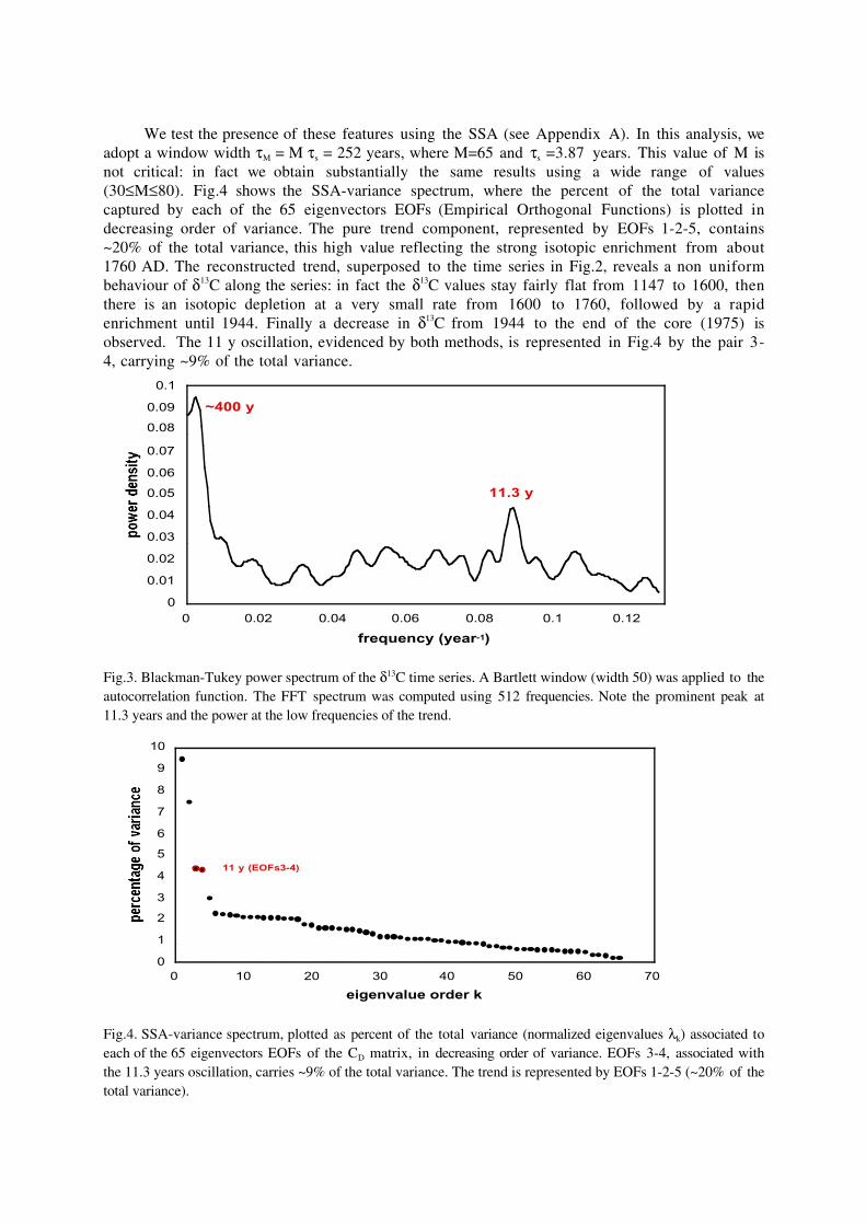
We test the presence of these features using the SSA (see Appendix A). In this analysis, weadopt a window width tM = M ts = 252 years, where M=65 and ts =3.87 years. This value of M isnot critical: in fact we obtain substantially the same results using a wide range of values(30£M£80). Fig.4 shows the SSA-variance spectrum, where the percent of the total variancecaptured by each of the 65 eigenvectors EOFs (Empirical Orthogonal Functions) is plotted indecreasing order of variance. The pure trend component, represented by EOFs 1-2-5, contains~20% of the total variance, this high value reflecting the strong isotopic enrichment from about1760 AD. The reconstructed trend, superposed to the time series in Fig.2, reveals a non uniformbehaviour of d13C along the series: in fact the d13C values stay fairly flat from 1147 to 1600, thenthere is an isotopic depletion at a very small rate from 1600 to 1760, followed by a rapidenrichment until 1944. Finally a decrease in d13C from 1944 to the end of the core (1975) isobserved. The 11 y oscillation, evidenced by both methods, is represented in Fig.4 by the pair 3-4, carrying ~9% of the total variance.

0

0.01

0.02

0.03

0.04

0.05

0.06

0.07

0.08

0.09

0.1

0 0.02 0.04 0.06 0.08 0.1 0.12

frequency (year-1)

11.3 y

~400 y

Fig.3. Blackman-Tukey power spectrum of the d13C time series. A Bartlett window (width 50) was applied to theautocorrelation function. The FFT spectrum was computed using 512 frequencies. Note the prominent peak at11.3 years and the power at the low frequencies of the trend.

0

1

2

3

4

5

6

7

8

9

10

0 10 20 30 40 50 60 70

eigenvalue order k

11 y (EOFs3-4)

Fig.4. SSA-variance spectrum, plotted as percent of the total variance (normalized eigenvalues lk) associated toeach of the 65 eigenvectors EOFs of the CD matrix, in decreasing order of variance. EOFs 3-4, associated withthe 11.3 years oscillation, carries ~9% of the total variance. The trend is represented by EOFs 1-2-5 (~20% of thetotal variance).

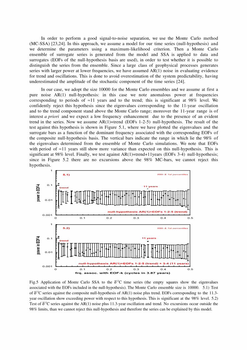
In order to perform a good signal-to-noise separation, we use the Monte Carlo method(MC-SSA) [23,24]. In this approach, we assume a model for our time series (null-hypothesis) andwe determine the parameters using a maximum-likelihood criterion. Then a Monte Carloensemble of surrogate series is generated from the model and SSA is applied to data andsurrogates (EOFs of the null-hypothesis basis are used), in order to test whether it is possible todistinguish the series from the ensemble. Since a large class of geophysical processes generatesseries with larger power at lower frequencies, we have assumed AR(1) noise in evaluating evidencefor trend and oscillations. This is done to avoid overestimation of the system predictability, havingunderestimated the amplitude of the stochastic component of the time series [24].

In our case, we adopt the size 10000 for the Monte Carlo ensembles and we assume at first apure noise AR(1) null-hypothesis: in this case we note anomalous power at frequenciescorresponding to periods of ª11 years and to the trend; this is significant at 98% level. Weconfidently reject this hypothesis since the eigenvalues corresponding to the 11-year oscillationand to the trend component stand above the Monte Carlo range; moreover the 11-year range is ofinterest a priori and we expect a low frequency enhancement due to the presence of an evidenttrend in the series. Now we assume AR(1)+trend (EOFs 1-2-5) null-hypothesis. The result of thetest against this hypothesis is shown in Figure 5.1, where we have plotted the eigenvalues and thesurrogate bars as a function of the dominant frequency associated with the corresponding EOFs ofthe composite null-hypothesis basis. The vertical bars indicate the range in which lie the 98% ofthe eigenvalues determined from the ensemble of Monte Carlo simulations. We note that EOFswith period of ª11 years still show more variance than expected on this null-hypothesis. This issignificant at 98% level. Finally, we test against AR(1)+trend+11years (EOFs 3-4) null-hypothesis;since in Figure 5.2 there are no excursions above the 98% MC-bars, we cannot reject thishypothesis.

0.001

0.01

0.1

1

0 0.1 0.2 0.3 0.4 0.5

5.1) 99th & 1st percentiles

null-hypothesis AR(1)+EOFs 1-2-5 (trend)

11 yearstrend

0.001

0.01

0.1

1

0 0.1 0.2 0.3 0.4 0.5

frq. assoc. with EOF-k (cycles in 3.87 years)

5.2) 99th & 1st percentiles

null-hypothesis AR(1)+EOFs 1-2-5 (trend) + 3-4 (11 years)

11 yearstrend

Fig.5 Application of Monte Carlo SSA to the d13C time series (the empty squares show the eigenvaluesassociated with the EOFs included in the null-hypothesis). The Monte Carlo ensemble size is 10000. 5.1) Testof d13C series against the composite null-hypothesis of AR(1) noise plus trend. EOFs corresponding to the 11.3-year oscillation show exceeding power with respect to this hypothesis. This is significant at the 98% level. 5.2)Test of d13C series against the AR(1) noise plus 11.3-year oscillation and trend. No excursions occur outside the98% limits, than we cannot reject this null-hypothesis and therefore the series can be explained by this model.

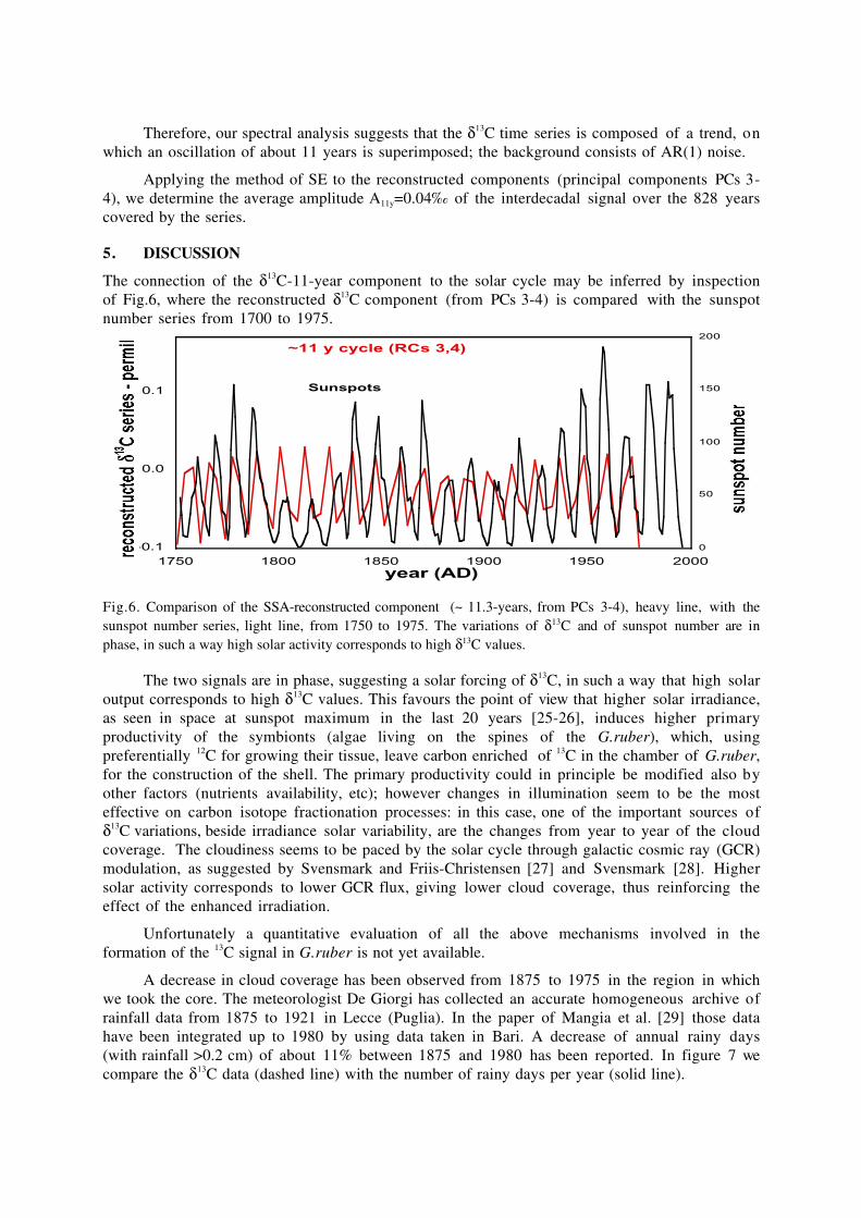
Therefore, our spectral analysis suggests that the d13C time series is composed of a trend, onwhich an oscillation of about 11 years is superimposed; the background consists of AR(1) noise.

Applying the method of SE to the reconstructed components (principal components PCs 3-4), we determine the average amplitude A11y=0.04‰ of the interdecadal signal over the 828 yearscovered by the series.

5. DISCUSSION

The connection of the d13C-11-year component to the solar cycle may be inferred by inspectionof Fig.6, where the reconstructed d13C component (from PCs 3-4) is compared with the sunspotnumber series from 1700 to 1975.

-0.1

0.0

0.1

1750 1800 1850 1900 1950 2000year (AD)

0

50

100

150

200

~11 y cycle (RCs 3,4)

Sunspots

Fig.6. Comparison of the SSA-reconstructed component (~ 11.3-years, from PCs 3-4), heavy line, with thesunspot number series, light line, from 1750 to 1975. The variations of d13C and of sunspot number are inphase, in such a way high solar activity corresponds to high d13C values.

The two signals are in phase, suggesting a solar forcing of d13C, in such a way that high solaroutput corresponds to high d13C values. This favours the point of view that higher solar irradiance,as seen in space at sunspot maximum in the last 20 years [25-26], induces higher primaryproductivity of the symbionts (algae living on the spines of the G.ruber), which, usingpreferentially 12C for growing their tissue, leave carbon enriched of 13C in the chamber of G.ruber,for the construction of the shell. The primary productivity could in principle be modified also byother factors (nutrients availability, etc); however changes in illumination seem to be the mosteffective on carbon isotope fractionation processes: in this case, one of the important sources ofd13C variations, beside irradiance solar variability, are the changes from year to year of the cloudcoverage. The cloudiness seems to be paced by the solar cycle through galactic cosmic ray (GCR)modulation, as suggested by Svensmark and Friis-Christensen [27] and Svensmark [28]. Highersolar activity corresponds to lower GCR flux, giving lower cloud coverage, thus reinforcing theeffect of the enhanced irradiation.

Unfortunately a quantitative evaluation of all the above mechanisms involved in theformation of the 13C signal in G.ruber is not yet available.

A decrease in cloud coverage has been observed from 1875 to 1975 in the region in whichwe took the core. The meteorologist De Giorgi has collected an accurate homogeneous archive ofrainfall data from 1875 to 1921 in Lecce (Puglia). In the paper of Mangia et al. [29] those datahave been integrated up to 1980 by using data taken in Bari. A decrease of annual rainy days(with rainfall >0.2 cm) of about 11% between 1875 and 1980 has been reported. In figure 7 wecompare the d13C data (dashed line) with the number of rainy days per year (solid line).

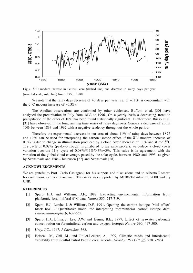
0.6

0.7

0.8

0.9

1

1.1

1.2

1.3

1860 1880 1900 1920 1940 1960 1980

year (AD)

dddd 13C

- GT9

0/340

50

60

70

80

90

100

110

120

130

140

rainy

days

per y

ear

Fig.7. d13C modern increase in GT90/3 core (dashed line) and decrease in rainy days per year

(inverted scale, solid line) from 1875 to 1980.

We note that the rainy days decrease of 40 days per year, i.e. of ~11%, is concomitant withthe d13C modern increase of ~0.3‰.

The Apulian observations are confirmed by other evidences. Buffoni et al. [30] haveanalysed the precipitation in Italy from 1833 to 1996. On a yearly basis a decreasing trend inprecipitation of the order of 10% has been found statistically significant. Furthermore Russo et al.[31] have observed in the long running time series of rainy days over Genova a decrease of about10% between 1833 and 1992 with a negative tendency throughout the whole period.

Therefore the experimental decrease in our area of about 11% of rainy days between 1875and 1980 can be used for interpreting the carbon isotope effect. If the d13C modern increase of0.3‰ is due to change in illumination produced by a cloud cover decrease of 11% and if the d13C11y cycle of 0.08‰ (peak-to-trough) is attributed to the same process, we deduce a cloud covervariation over the 11-y cycle of 0.08‰*11%/0.3‰=3%. This value is in agreement with thevariation of the global cloud coverage, paced by the solar cycle, between 1980 and 1995, as givenby Svensmark and Friis-Chrstensen [27] and Svensmark [28].

ACKNOWLEDGEMENTS

We are grateful to Prof. Carlo Castagnoli for his support and discussions and to Alberto Romerofor continuous technical assistance. This work was supported by MURST-Co-fin 98, 2000 and byCNR.

REFERENCES

[1] Spero, H.J. and Williams, D.F., 1988, Extracting environmental information fromplanktonic foraminiferal d13C data, Nature 335, 717-719.

[2] Spero, H.J., Lerche, J. & Williams, D.F., 1991, Opening the carbon isotope "vital effect"black box, 2: Quantitative model for interpreting foraminiferal carbon isotope data.Paleoceanography 6, 639-655.

[3] Spero, H.J., Bijma, J., Lea, D.W. and Bemis, B.E., 1997, Effect of seawater carbonateconcentration on foraminiferal carbon and oxygen isotopes Nature 390, 497-500.

[4] Urey, J.C., 1947, J.Chem.Soc. 562.

[5] Boiseau, M,, Ghil, M., and Juillet-Leclerc, A., 1999, Climatic trends and interdecadalvariability from South-Central Pacific coral records, Geophys.Res.Lett. 26, 2281-2884.

[6] Cini Castagnoli, G., Bonino, G., Caprioglio, F., Provenzale, A., Serio, M. & Zhu, G.M.,1990, The carbonate profile of two recent Ionian sea cores: evidence that thesedimentation rate is constant over the last Millennia Geophys.Res.Lett. 17, 1937-1940.

[7] Cini Castagnoli, G., Bonino, Provenzale, A., Serio, M. & Callegari, E., 1992a, The CaCO3profiles of deep and shallow Mediterranean sea cores as indicators of past solar-terrestrialrelationships, Nuovo Cimento C15, 547-563.

[8] Cini Castagnoli, G., Bonino, G., Serio, M. & Sonett, C.P., 1992b, Common spectral featuresin the 5500-year record of total carbonate in sea sediments and Radiocarbon in tree rings.Radiocarbon 34, 798-805.

[9] Bonino, G., Cini Castagnoli, G., Callegari E., and Zhu, G.M., 1993, Radiometric andtephroanalysis dating of Recent Ionian Sea cores, Nuovo Cimento C 16, 155-161.

[10] Arno’, V., Principe, C., Rosi, M., Santacroce, R., Sbrana, A. and Sheridan M.F., 1987,Eruptive History, in Summa-Vesuvius, Quaderni de La Ricerca Scientifica, CNR, 114, (ed.Santacroce R.) 53-103.

[11] Cini Castagnoli, G., 1997, The 200y variability in terrrestrial archives: solar forcing? inPast and Present variability of the Solar-Terrestrial System: measurements, data analysisand theoretical models (eds. Cini Castagnoli, G. and Provenzale, A. 47-57, I0S press,Amsterdam).

[12] Cini Castagnoli, G., Bernasconi, S.M., Bonino, G., Della Monica, P., Taricco, C., 1999a,700 year record of the 11 year solar cycle by planktonic foraminifera of a shallow waterMediterranean core, Adv. Space Res. 24, 233-236.

[13] Cini Castagnoli, G., Bernasconi, S.M., Bonino, G., Della Monica, P., and Taricco, C.,1999b, Solar activity in the last millennium recorded in the d18O profile of planktonicforaminifera of a shallow water Ionian sea core, Sol. Phys. 188, 191-202.

[14] Cini Castagnoli, G., Bonino, G., Taricco, C., 2001, Long term solar-terrestrial records fromsediments: carbon isotopes in planktonic foraminifera in the last millennium, Adv. SpaceRes., in press.

[15] Beveridge, N.A.S., and Shackleton, N.J., 1994, Carbon isotopes in recent planktonicforaminifera: a record of anthropogenic CO2 invasion of the surface ocean, Earth andPlanet. Sci. Lett. 126, 259-273.

[16] Spero, H.J. and Lea, D.W., 1993, Intraspecific stable isotope variability in the planktonicforaminifera Globigerinoides sacculifer: Results from laboratory experiments. Mar.Micropaleontol. 22, 221-234.0

[17] Ghil, M., and Taricco, C., 1997, Advanced spectral-analysis methods, in Past and PresentVariability of the Solar-terrestrial System: Measurement, Data Analysis and TheoreticalModels Proc. of the Int. School of Physics E.Fermi, Varenna, 1996, Course CXXXIII,edited by G.Cini Castagnoli and A.Provenzale (IOS Press, Amsterdam), p.137-159.

[18] Blackman, R.B., and Tukey, J.W., 1958, The Measurement of Power Spectra from thePoint of View of Communication Engineering (Dover, New York).

[19] Kay, S.M., 1988, Modern Spectral Estimation: Theory and Applications (Prentice-Hall,Cliffs, N.J.).

[20] Broomhead, D.S., and King, G.P., 1986, Extracting qualitative dynamics fromexperimental data, Physica D 20, 217-236.

[21] Vautard, R., and Ghil, M., 1989, Singular spectrum analysis in nonlinear dynamics, withapplications to paleoclimatic time series, Physica D 35, 395-424.

[22] Dettinger, M.D., Ghil, M., Strong, C.M., Weibel, W., and Yiou, P., 1995, Software expeditessingular-spectrum analysis of noisy time serie, EOS Trans. AGU, 76, 12.

[23] Allen, M.R., 1992, Interactions between the atmosphere and oceans on timescales of weeksto years, PhD Thesis, Clarendon Laboratory, Oxford.

[24] Allen, M.R., and Smith, L.A., 1996, Monte Carlo SSA: detecting irregular oscillations inthe presence of coloured noise, J.Clim.9, 3373.

[25] Willson, R.C., and Hudson, H.S., 1991, The Sun’s luminosity over a complete solar cycle,Nature 351, 42-44.

[26] Pap, J.M., 1997, in Past and Present Variability of the Solar-terrestrial System:Measurement, Data Analysis and Theoretical Models, Proc. of the Int. School of PhysicsE.Fermi, Varenna, 1996, Course CXXXIII, edited by G.Cini Castagnoli and A.Provenzale(IOS Press, Amsterdam), p.1-24.

[27] Svensmark, H., and Friis-Christensen, E., 1997, Variation of cosmic ray flux and globalcloud coverage- a missing link in solar-climate relationships, J.Atmos.Sol.Terr.Phys. 59,1225-1232.

[28] Svensmark, H., 1998, Influence of cosmic rays on Earthís climate, Phys.Rev.Lett., 81,5027-5030.

[29] Mangia, C., De Sanctis, L.V., Ruggiero, L., Zito, G., Zuanni, F., 1991, Un secolo diprecipitazioni piovose a Lecce, 4th Workshop Progetto strategico: Clima, ambiente eterritorio nel mezzogiorno, ISIATA-CNR, Lecce, 153-161.

[30] Buffoni, L., Maugeri, M., Nanni, T., 1999, Precipitation in Italy from 1833 to 1996, Teor.Appl. Climatol. 63, 33-40.

[31] G.Russo, C.Eva, C.Palau, A.Caneva and A.Sacchini, 2000, Nuovo Cimento, C23, 39-52.

[32] Vautard, R., Yiou, P., and Ghil, M., 1992, Singular Spectrum Analysis: a toolkit for short,noisy, chaotic time series, Physica D58, 95-126.

APPENDIX 1The SSA approach involves 3 basic steps: 1) embedding the time series in a vector spaceof dimension M (for the choice of M, see Ref.[32]); 2) computing the MxM lag-covariance matrix CD of the data (see the two different approach of Broomhead andKing [20] and of Vautard and Ghil, [21]); 3) diagonalising CD :

LD = EDT CDED ,

where LD = diag(l1,l2,...,lM ) , with l1 ≥ l2 ≥...≥ lM ≥ 0 and ED is the MxMmatrix having the corresponding eigenvectors Ek , k=1,...,M as its columns. For each Ek

we construct the time series (of length N-M+1), called k-th principal component (PC),representing the projection of the original time series in the direction determined by theeigenvector Ek (also called empirical orthogonal function, EOF). Each eigenvalue lkgives the variance of the corresponding PC; its square root is called singular value (SV).Having chosen a subset of eigenvalues, it is possible to extract time series of length N,combining PCs; these time series are called reconstructed components (RCs) and theycan be superimposed to the original signal.

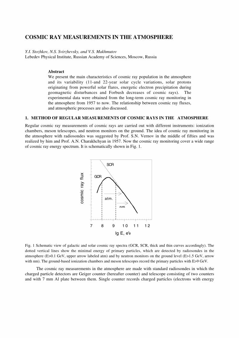
COSMIC RAY MEASUREMENTS IN THE ATMOSPHERE

Y.I. Stozhkov, N.S. Svirzhevsky, and V.S. MakhmutovLebedev Physical Institute, Russian Academy of Sciences, Moscow, Russia

AbstractWe present the main characteristics of cosmic ray population in the atmosphereand its variability (11-and 22-year solar cycle variations, solar protonsoriginating from powerful solar flares, energetic electron precipitation duringgeomagnetic disturbances and Forbush decreases of cosmic rays). Theexperimental data were obtained from the long-term cosmic ray monitoring inthe atmosphere from 1957 to now. The relationship between cosmic ray fluxes,and atmospheric processes are also discussed.

1. METHOD OF REGULAR MEASUREMENTS OF COSMIC RAYS IN THE ATMOSPHERE

Regular cosmic ray measurements of cosmic rays are carried out with different instruments: ionizationchambers, meson telescopes, and neutron monitors on the ground. The idea of cosmic ray monitoring inthe atmosphere with radiosondes was suggested by Prof. S.N. Vernov in the middle of fifties and wasrealized by him and Prof. A.N. Charakhchyan in 1957. Now the cosmic ray monitoring cover a wide rangeof cosmic ray energy spectrum. It is schematically shown in Fig. 1.

1

2

3

4

5

7 8 9 1 0 1 1 1 2

lg E, eV

cosm

ic r

ay f

lux

GCR

SCR

nm

atm.

Fig. 1 Schematic view of galactic and solar cosmic ray spectra (GCR, SCR, thick and thin curves accordingly). Thedotted vertical lines show the minimal energy of primary particles, which are detected by radiosondes in theatmosphere (E>0.1 GeV, upper arrow labeled atm) and by neutron monitors on the ground level (E>1.5 GeV, arrowwith nm). The ground-based ionization chambers and meson telescopes record the primary particles with E>9 GeV.

The cosmic ray measurements in the atmosphere are made with standard radiosondes in which thecharged particle detectors are Geiger counter (hereafter counter) and telescope consisting of two countersand with 7 mm Al plate between them. Single counter records charged particles (electrons with energy

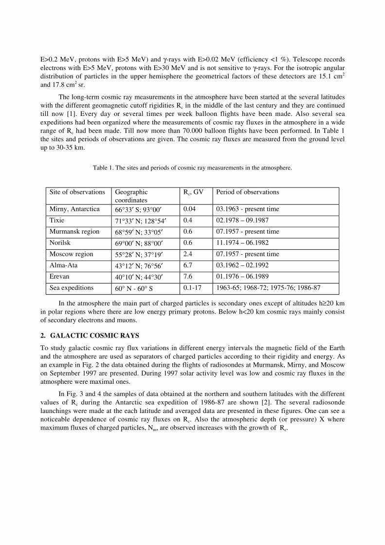
E>0.2 MeV, protons with E>5 MeV) and g-rays with E>0.02 MeV (efficiency <1 %). Telescope recordselectrons with E>5 MeV, protons with E>30 MeV and is not sensitive to g-rays. For the isotropic angulardistribution of particles in the upper hemisphere the geometrical factors of these detectors are 15.1 cm2

and 17.8 cm2 sr.

The long-term cosmic ray measurements in the atmosphere have been started at the several latitudeswith the different geomagnetic cutoff rigidities Rc in the middle of the last century and they are continuedtill now [1]. Every day or several times per week balloon flights have been made. Also several seaexpeditions had been organized where the measurements of cosmic ray fluxes in the atmosphere in a widerange of Rc had been made. Till now more than 70.000 balloon flights have been performed. In Table 1the sites and periods of observations are given. The cosmic ray fluxes are measured from the ground levelup to 30-35 km.

Table 1. The sites and periods of cosmic ray measurements in the atmosphere.

Site of observations Geographiccoordinates

Rc, GV Period of observations

Mirny, Antarctica 66∞33¢ S; 93∞00¢ 0.04 03.1963 - present time

Tixie 71∞33¢ N; 128∞54¢ 0.4 02.1978 – 09.1987

Murmansk region 68∞59¢ N; 33∞05¢ 0.6 07.1957 - present time

Norilsk 69∞00¢ N; 88∞00¢ 0.6 11.1974 – 06.1982

Moscow region 55∞28¢ N; 37∞19¢ 2.4 07.1957 - present time

Alma-Ata 43∞12¢ N; 76∞56¢ 6.7 03.1962 – 02.1992

Erevan 40∞10¢ N; 44∞30¢ 7.6 01.1976 – 06.1989

Sea expeditions 60∞ N - 60∞ S 0.1-17 1963-65; 1968-72; 1975-76; 1986-87

In the atmosphere the main part of charged particles is secondary ones except of altitudes h≥20 kmin polar regions where there are low energy primary protons. Below h<20 km cosmic rays mainly consistof secondary electrons and muons.

2. GALACTIC COSMIC RAYS

To study galactic cosmic ray flux variations in different energy intervals the magnetic field of the Earthand the atmosphere are used as separators of charged particles according to their rigidity and energy. Asan example in Fig. 2 the data obtained during the flights of radiosondes at Murmansk, Mirny, and Moscowon September 1997 are presented. During 1997 solar activity level was low and cosmic ray fluxes in theatmosphere were maximal ones.

In Fig. 3 and 4 the samples of data obtained at the northern and southern latitudes with the differentvalues of Rc during the Antarctic sea expedition of 1986-87 are shown [2]. The several radiosondelaunchings were made at the each latitude and averaged data are presented in these figures. One can see anoticeable dependence of cosmic ray fluxes on Rc. Also the atmospheric depth (or pressure) X wheremaximum fluxes of charged particles, Nm, are observed increases with the growth of Rc.

The examples of the time dependencies of charged particle fluxes (monthly averaged values)measured at the polar (northern and southern) and middle latitudes in the stratosphere and troposphere aregiven in Fig. 5 and 6. The period of observations covers ~19-23 solar activity cycles.

Fig. 2. The count rate of single counter vs. altitude in the atmosphere: at the northern polar latitude, Murmanskregion, Rc=0.6 GV (the radiosonde flights on 2 and 4 September 1997 - open circles and black points, accordingly);at Mirny in the Antarctic, Rc=0.04 GV (the flights on 3 and 8 September - open and black triangles, accordingly); atthe middle latitude, Moscow region, Rc=2.4 GV (the flight on 3 September - open squares).

Fig. 3. The cosmic ray fluxes vs. atmospheric pressure X measured at different latitudes of the northern hemisphere during the sea

expedition of 1986-1987. The values of Rc in GV are shown for each curve. The vertical bars show standard errors.

0

5

1 0

1 5

2 0

2 5

3 0

3 5

4 0

0 1000 2000 3000 4000

N, min-1

h, k

m

0.0

0.5

1.0

1.5

2.0

2.5

3.0

3.5

1 10 100 1000

X, g cm-2

N, c

m-2

s-1

0.6

2.4

north

6.7

10.713.7

5.3

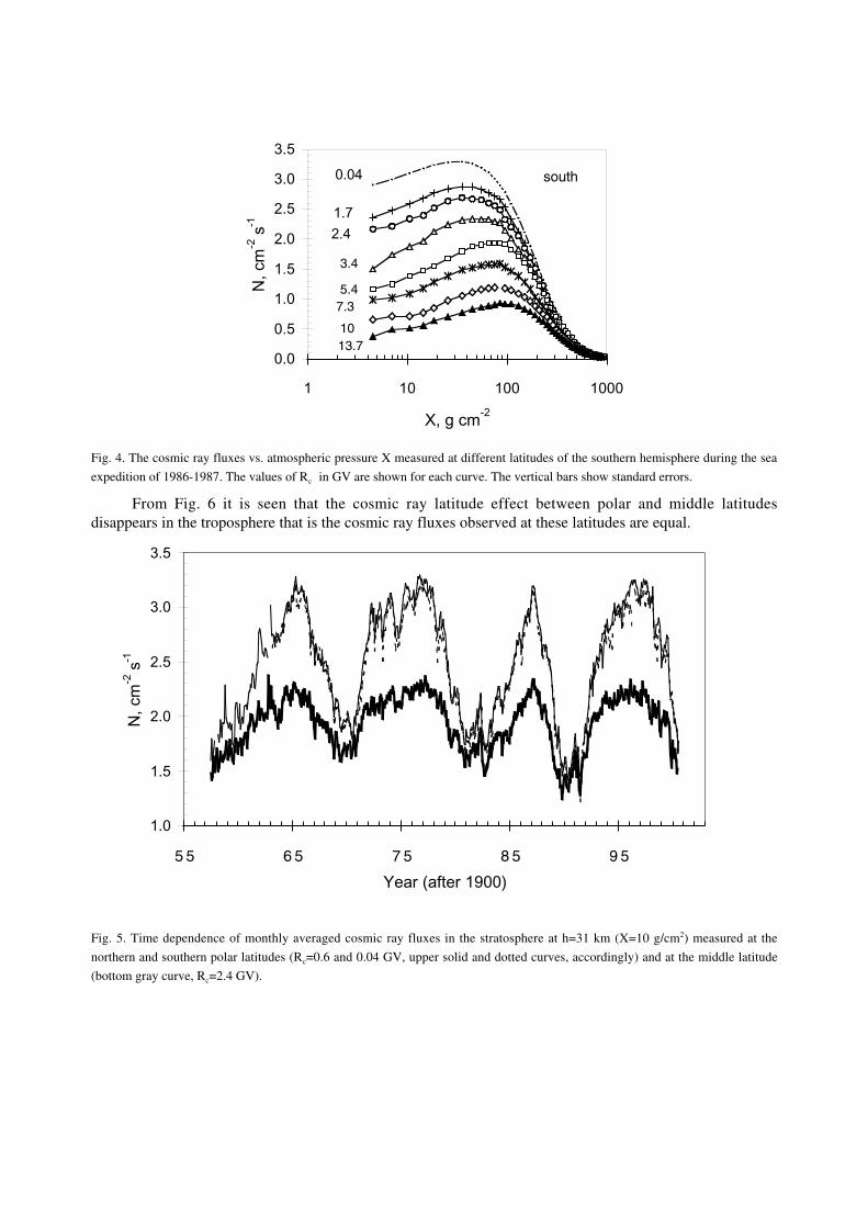
Fig. 4. The cosmic ray fluxes vs. atmospheric pressure X measured at different latitudes of the southern hemisphere during the sea

expedition of 1986-1987. The values of Rc in GV are shown for each curve. The vertical bars show standard errors.

From Fig. 6 it is seen that the cosmic ray latitude effect between polar and middle latitudesdisappears in the troposphere that is the cosmic ray fluxes observed at these latitudes are equal.

Fig. 5. Time dependence of monthly averaged cosmic ray fluxes in the stratosphere at h=31 km (X=10 g/cm2) measured at the

northern and southern polar latitudes (Rc=0.6 and 0.04 GV, upper solid and dotted curves, accordingly) and at the middle latitude

(bottom gray curve, Rc=2.4 GV).

0.0

0.5

1.0

1.5

2.0

2.5

3.0

3.5

1 10 100 1000

X, g cm-2

N, c

m-2

s-1

0.04

1.7

2.4

south

3.4

5.47.3

1013.7

1.0

1.5

2.0

2.5

3.0

3.5

5 5 6 5 7 5 8 5 9 5

Year (after 1900)

N, c

m-2

s-1

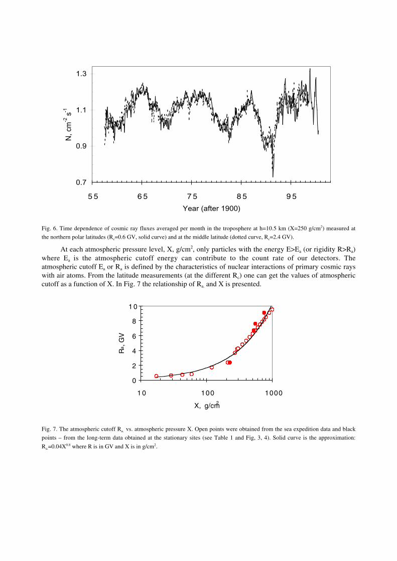
Fig. 6. Time dependence of cosmic ray fluxes averaged per month in the troposphere at h=10.5 km (X=250 g/cm2) measured at

the northern polar latitudes (Rc=0.6 GV, solid curve) and at the middle latitude (dotted curve, Rc=2.4 GV).

At each atmospheric pressure level, X, g/cm2, only particles with the energy E>Ea (or rigidity R>Ra)where Ea is the atmospheric cutoff energy can contribute to the count rate of our detectors. Theatmospheric cutoff Ea or Ra is defined by the characteristics of nuclear interactions of primary cosmic rayswith air atoms. From the latitude measurements (at the different Rc) one can get the values of atmosphericcutoff as a function of X. In Fig. 7 the relationship of Ra. and X is presented.

0

2

4

6

8

1 0

1 0 100 1000

X, g/cm2

Ra, G

V

Fig. 7. The atmospheric cutoff Ra. vs. atmospheric pressure X. Open points were obtained from the sea expedition data and black

points – from the long-term data obtained at the stationary sites (see Table 1 and Fig, 3, 4). Solid curve is the approximation:

Ra.=0.04X0.8 where R is in GV and X is in g/cm2.

0.7

0.9

1.1

1.3

5 5 6 5 7 5 8 5 9 5

Year (after 1900)

N, c

m-2

s-1

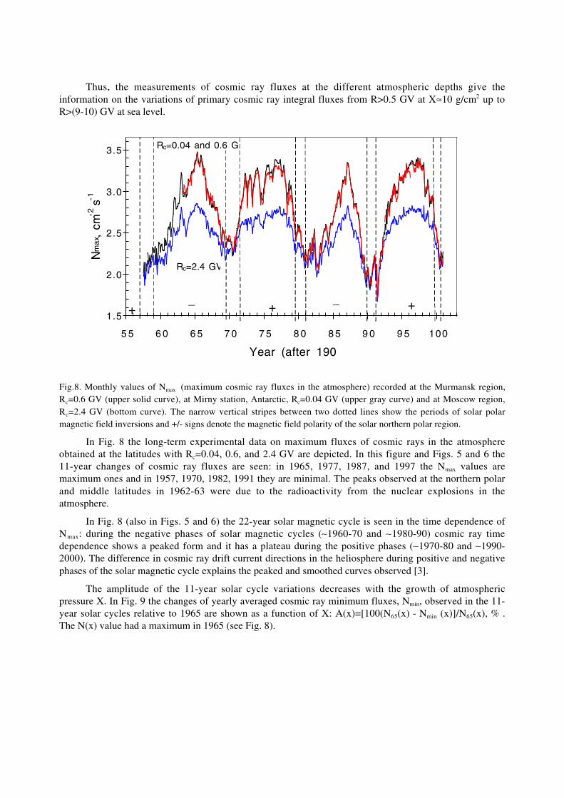
Thus, the measurements of cosmic ray fluxes at the different atmospheric depths give theinformation on the variations of primary cosmic ray integral fluxes from R>0.5 GV at Xª10 g/cm2 up toR>(9-10) GV at sea level.

Fig.8. Monthly values of Nmax (maximum cosmic ray fluxes in the atmosphere) recorded at the Murmansk region,Rc=0.6 GV (upper solid curve), at Mirny station, Antarctic, Rc=0.04 GV (upper gray curve) and at Moscow region,Rc=2.4 GV (bottom curve). The narrow vertical stripes between two dotted lines show the periods of solar polarmagnetic field inversions and +/- signs denote the magnetic field polarity of the solar northern polar region.

In Fig. 8 the long-term experimental data on maximum fluxes of cosmic rays in the atmosphereobtained at the latitudes with Rc=0.04, 0.6, and 2.4 GV are depicted. In this figure and Figs. 5 and 6 the11-year changes of cosmic ray fluxes are seen: in 1965, 1977, 1987, and 1997 the Nmax values aremaximum ones and in 1957, 1970, 1982, 1991 they are minimal. The peaks observed at the northern polarand middle latitudes in 1962-63 were due to the radioactivity from the nuclear explosions in theatmosphere.

In Fig. 8 (also in Figs. 5 and 6) the 22-year solar magnetic cycle is seen in the time dependence ofNmax: during the negative phases of solar magnetic cycles (~1960-70 and ~1980-90) cosmic ray timedependence shows a peaked form and it has a plateau during the positive phases (~1970-80 and ~1990-2000). The difference in cosmic ray drift current directions in the heliosphere during positive and negativephases of the solar magnetic cycle explains the peaked and smoothed curves observed [3].

The amplitude of the 11-year solar cycle variations decreases with the growth of atmosphericpressure X. In Fig. 9 the changes of yearly averaged cosmic ray minimum fluxes, Nmin, observed in the 11-year solar cycles relative to 1965 are shown as a function of X: A(x)=[100(N65(x) - Nmin (x)]/N65(x), % .The N(x) value had a maximum in 1965 (see Fig. 8).

1.5

2.0

2.5

3.0

3.5

5 5 6 0 6 5 7 0 7 5 8 0 8 5 9 0 9 5 100

Year (after 190

Nm

ax,

cm-2

s-1

Rc=2.4 GV

Rc=0.04 and 0.6 G

+ ++__

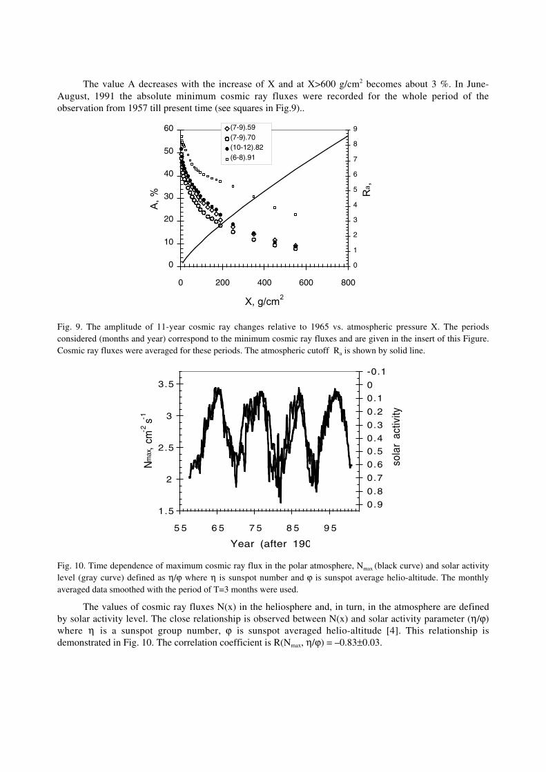
The value A decreases with the increase of X and at X>600 g/cm2 becomes about 3 %. In June-August, 1991 the absolute minimum cosmic ray fluxes were recorded for the whole period of theobservation from 1957 till present time (see squares in Fig.9)..

Fig. 9. The amplitude of 11-year cosmic ray changes relative to 1965 vs. atmospheric pressure X. The periodsconsidered (months and year) correspond to the minimum cosmic ray fluxes and are given in the insert of this Figure.Cosmic ray fluxes were averaged for these periods. The atmospheric cutoff Ra is shown by solid line.

Fig. 10. Time dependence of maximum cosmic ray flux in the polar atmosphere, Nmax (black curve) and solar activitylevel (gray curve) defined as h/j where h is sunspot number and j is sunspot average helio-altitude. The monthlyaveraged data smoothed with the period of T=3 months were used.

The values of cosmic ray fluxes N(x) in the heliosphere and, in turn, in the atmosphere are definedby solar activity level. The close relationship is observed between N(x) and solar activity parameter (h/j)where h is a sunspot group number, j is sunspot averaged helio-altitude [4]. This relationship isdemonstrated in Fig. 10. The correlation coefficient is R(Nmax, h/j) = –0.83±0.03.

0

10

20

30

40

50

60

0 200 400 600 800

X, g/cm2

A, %

0

1

2

3

4

5

6

7

8

9

Ra ,

(7-9).59(7-9).70(10-12).82(6-8).91

1.5

2

2.5

3

3.5

5 5 6 5 7 5 8 5 9 5

Year (after 190

Nm

ax,

cm-2

s-1

-0.1

0

0.1

0.2

0.3

0.4

0.5

0.6

0.7

0.8

0.9

sola

r ac

tivity

The galactic cosmic ray modulation in the heliosphere is produced by magnetic irregularities ofinterplanetary magnetic field (IMF). In turn, the value of IMF and its irregularity density are defined bysolar activity. The density of these irregularities increases with the growth of IMF strength. So, we canexpect a relationship between IMF strength and cosmic ray fluxes in the heliosphere as well as in theatmosphere. This relationship is given in Fig. 11. The correlation coefficient R(Nmax, IMF)= -0.71±0.04.

Fig.11. Time dependence of maximum cosmic ray flux in the polar atmosphere, Nmax (black curve) and IMF (graycurve). The monthly averaged data smoothed with the period of T=3 months were used. The data on IMF were takenfrom INTERNET: http://nssdc.gsfc.nasa.gov/omniweb/.

Fig. 12. Cosmic ray fluxes recorded in the atmosphere at Mirny in the Antarctic during the solar proton event on 9November 2000. Solid curve is a charged particle flux background produced by galactic cosmic rays in theatmosphere (GCR). Different symbols show the data obtained during the different flights of radiosondes (the dateand start time of launchings are given in the insert)..

1.5

2

2.5

3

3.5

5 5 6 5 7 5 8 5 9 5

Year (after 190

Nm

ax,

cm-2

s-1

4

5

6

7

8

9

1 0

1 1

IMF,

0

5

1 0

1 5

2 0

2 5

3 0

0.1 1.0 10.0 100.0

N, cm-2 s-1

h, k

m

GCR

0822 11.09.0

1053 11.09.0

1942 11.09.0

0326 11.10.0

Start time, UT, date

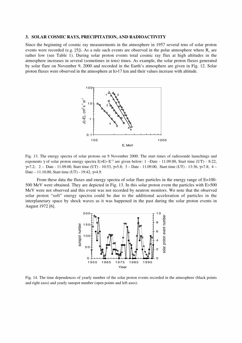
3. SOLAR COSMIC RAYS, PRECIPITATION, AND RADIOACTIVITY

Since the beginning of cosmic ray measurements in the atmosphere in 1957 several tens of solar protonevents were recorded (e.g. [5]). As a rule such events are observed in the polar atmosphere where Rc arerather low (see Table 1). During solar proton events total cosmic ray flux at high altitudes in theatmosphere increases in several (sometimes in tens) times. As example, the solar proton fluxes generatedby solar flare on November 9, 2000 and recorded in the Earth’s atmosphere are given in Fig. 12. Solarproton fluxes were observed in the atmosphere at h>17 km and their values increase with altitude.

Fig. 13. The energy spectra of solar protons on 9 November 2000. The start times of radiosonde launchings andexponents g of solar proton energy spectra I(>E)~E-g are given below: 1 –Date - 11.09.00, Start time (UT) - 8:22,g=7.2; 2 – Date - 11.09.00, Start time (UT) - 10:53, g=5.8; 3 – Date - 11.09.00, Start time (UT) - 13:36, g=7.8; 4 –Date – 11.10.00, Start time (UT) - 19:42, g=4.9.

From these data the fluxes and energy spectra of solar flare particles in the energy range of E=100-500 MeV were obtained. They are depicted in Fig. 13. In this solar proton event the particles with E>500MeV were not observed and this event was not recorded by neutron monitors. We note that the observedsolar proton “soft” energy spectra could be due to the additional acceleration of particles in theinterplanetary space by shock waves as it was happened in the past during the solar proton events inAugust 1972 [6].

Fig. 14. The time dependences of yearly number of the solar proton events recorded in the atmosphere (black pointsand right axes) and yearly sunspot number (open points and left axes).

0.1

1

1 0

100

100 1000

E, MeV

J(>E

), cm

-2 s

-1 s

r-1

1

2

3

4

0

5 0

100

150

200

1955 1965 1975 1985 1995

Year

suns

pot n

umbe

r

0

2

4

6

8

1 0

sola

r pr

oton

eve

nt n

umbe

r

For the 45-year period of cosmic ray monitoring in the atmosphere 105 solar proton events wererecorded. In Fig. 14 the time dependence of the yearly number of these events and solar activity level(sunspot number) are shown. It is seen that the solar proton events mainly occur during the ascending anddescending phases of solar activity.

0

5

1 0

1 5

2 0

2 5

3 0

3 5

0 1 2 3 4

N, cm-2 s-1

h, k

m

1250 05.03.0

0930 05.05.0

Start time UT Date

0

5

1 0

1 5

2 0

2 5

3 0

3 5

0 1 2 3

N, cm-2 s-1h,

km

1250 05.03.0

0930 05.05.0

Start time UT Date

Fig. 15. Precipitation of high energy electrons into the northern polar atmosphere recorded by single counter on 5March 2000 (left panel, black points). The background from galactic cosmic rays is shown by open points. Thetelescope recorded galactic cosmic ray background only (right panel). The inserts show the dates of radiosondeflights and launching times.

During the geomagnetic disturbed periods in the polar atmosphere at high altitudes high-energyelectron precipitation events are detected [7, 8, 9]. Our northern polar station in Murmansk region is nearthe polar oval (McIlwain’s parameter L=5.6) where the precipitations are observed rather often. In Fig. 15the example of precipitation detected on November 2000 is shown. The counter records secondary g-raysproduced by precipitating electrons in the atmosphere..

But at the same time the telescope records only the background from galactic cosmic rays and itallows to separate precipitation from solar proton events. It is significant that g-rays recorded in theatmosphere at h=25-35 km are produced by the precipitating electrons with E>several MeV. The timedependence of the yearly precipitation number and the sunspot number are given in Fig. 16. Into theprecipitation data the corrections for patrol efficiency were introduced. The data obtained show that theprecipitation take place most often during the descending phase of solar activity (remind that solar protonevents are observed most often during the ascending and descending solar activity phases, see Fig. 14).This fact was established earlier in other papers [10]. The total number of precipitation recorded at thestation in Murmansk region during 1957-2000 equals 549 events. For almost the same period (1963-2000)at the Antarctic station Mirny (66∞33 ¢ S; 93∞00¢; Rc=0.04 GV; Lª11) 10 precipitation events wererecorded only.

In Table 2 the yearly precipitation numbers for 20 - 23rd solar cycles are given. The last line in thisTable includes the ascending phase of 23rd solar activity cycle only.

The regular monitoring of charged particle fluxes in the atmosphere provides the prompt control ofradiation conditions and allows to detect radiation clouds from nuclear explosions or nuclear plantfailures. In Fig. 17 and 18 the observations of radioactive clouds in the polar northern atmosphere and

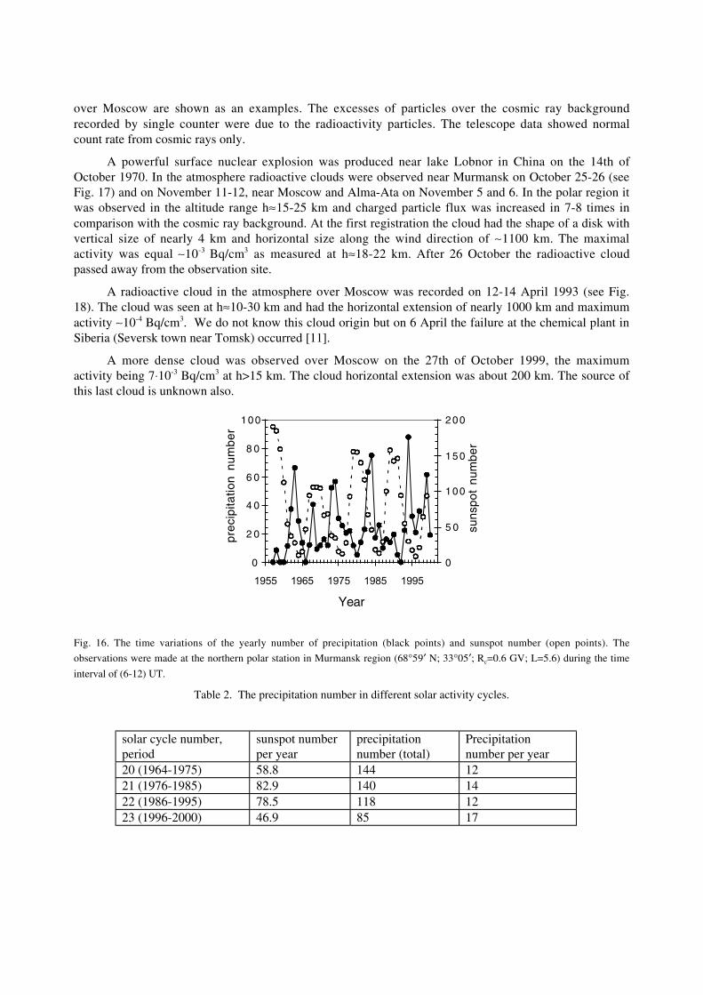
over Moscow are shown as an examples. The excesses of particles over the cosmic ray backgroundrecorded by single counter were due to the radioactivity particles. The telescope data showed normalcount rate from cosmic rays only.

A powerful surface nuclear explosion was produced near lake Lobnor in China on the 14th ofOctober 1970. In the atmosphere radioactive clouds were observed near Murmansk on October 25-26 (seeFig. 17) and on November 11-12, near Moscow and Alma-Ata on November 5 and 6. In the polar region itwas observed in the altitude range hª15-25 km and charged particle flux was increased in 7-8 times incomparison with the cosmic ray background. At the first registration the cloud had the shape of a disk withvertical size of nearly 4 km and horizontal size along the wind direction of ~1100 km. The maximalactivity was equal ~10-3 Bq/cm3 as measured at hª18-22 km. After 26 October the radioactive cloudpassed away from the observation site.

A radioactive cloud in the atmosphere over Moscow was recorded on 12-14 April 1993 (see Fig.18). The cloud was seen at hª10-30 km and had the horizontal extension of nearly 1000 km and maximumactivity ~10-4 Bq/cm3. We do not know this cloud origin but on 6 April the failure at the chemical plant inSiberia (Seversk town near Tomsk) occurred [11].

A more dense cloud was observed over Moscow on the 27th of October 1999, the maximumactivity being 7◊10-3 Bq/cm3 at h>15 km. The cloud horizontal extension was about 200 km. The source ofthis last cloud is unknown also.

Fig. 16. The time variations of the yearly number of precipitation (black points) and sunspot number (open points). The

observations were made at the northern polar station in Murmansk region (68∞59¢ N; 33∞05¢; Rc=0.6 GV; L=5.6) during the time

interval of (6-12) UT.

Table 2. The precipitation number in different solar activity cycles.

solar cycle number,period

sunspot numberper year

precipitationnumber (total)

Precipitationnumber per year

20 (1964-1975) 58.8 144 1221 (1976-1985) 82.9 140 1422 (1986-1995) 78.5 118 1223 (1996-2000) 46.9 85 17

0

2 0

4 0

6 0

8 0

100

1955 1965 1975 1985 1995

Year

prec

ipita

tion

num

ber

0

5 0

100

150

200

suns

pot

num

ber

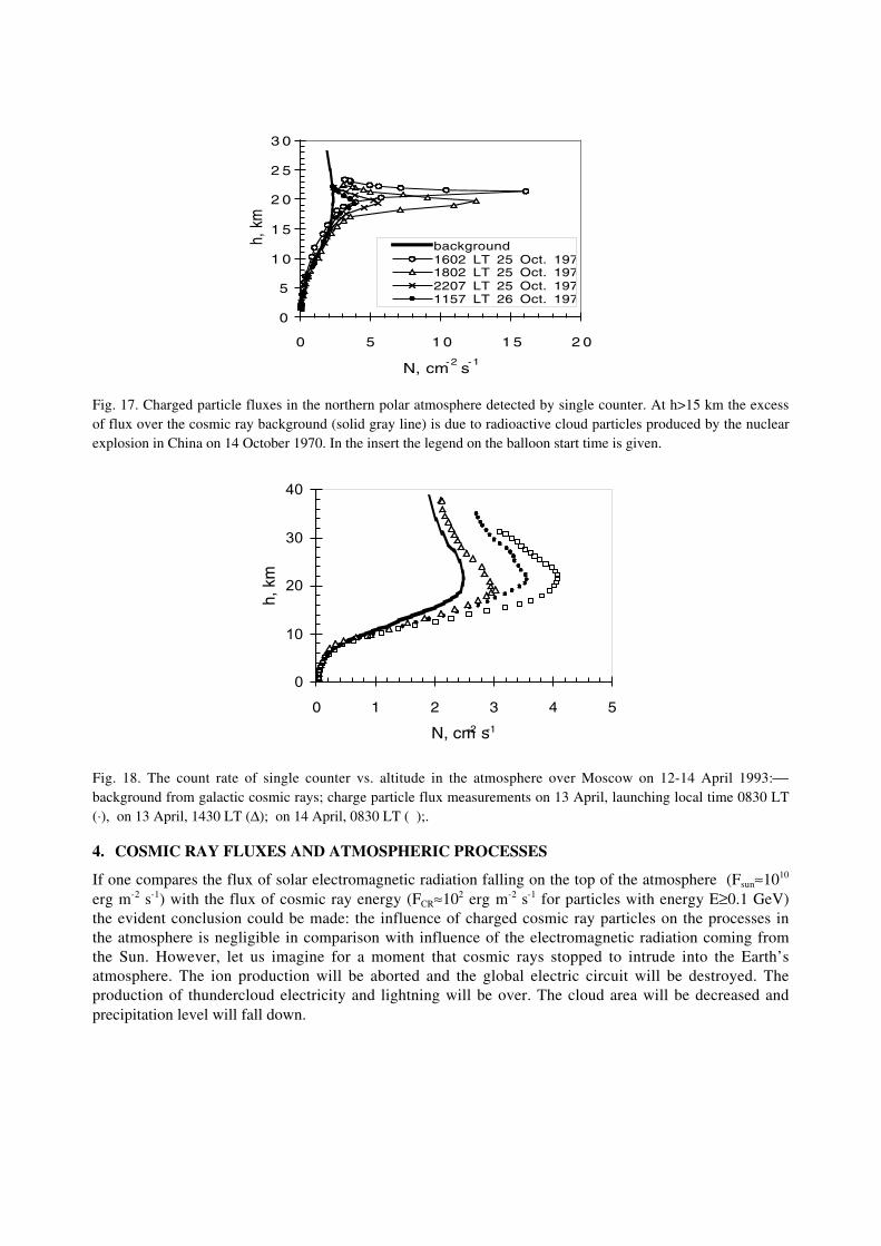
Fig. 17. Charged particle fluxes in the northern polar atmosphere detected by single counter. At h>15 km the excessof flux over the cosmic ray background (solid gray line) is due to radioactive cloud particles produced by the nuclearexplosion in China on 14 October 1970. In the insert the legend on the balloon start time is given.

Fig. 18. The count rate of single counter vs. altitude in the atmosphere over Moscow on 12-14 April 1993:æbackground from galactic cosmic rays; charge particle flux measurements on 13 April, launching local time 0830 LT(◊), on 13 April, 1430 LT (D); on 14 April, 0830 LT ( );.

4. COSMIC RAY FLUXES AND ATMOSPHERIC PROCESSES

If one compares the flux of solar electromagnetic radiation falling on the top of the atmosphere (Fsunª1010

erg m-2 s-1) with the flux of cosmic ray energy (FCRª102 erg m-2 s-1 for particles with energy E≥0.1 GeV)the evident conclusion could be made: the influence of charged cosmic ray particles on the processes inthe atmosphere is negligible in comparison with influence of the electromagnetic radiation coming fromthe Sun. However, let us imagine for a moment that cosmic rays stopped to intrude into the Earth’satmosphere. The ion production will be aborted and the global electric circuit will be destroyed. Theproduction of thundercloud electricity and lightning will be over. The cloud area will be decreased andprecipitation level will fall down.

0

5

1 0

1 5

2 0

2 5

3 0

0 5 1 0 1 5 2 0

N, cm-2

s-1

h, k

mbackground1602 LT 25 Oct. 1971802 LT 25 Oct. 1972207 LT 25 Oct. 1971157 LT 26 Oct. 197

0

10

20

30

40

0 1 2 3 4 5

N, cm-2 s-1

h, k

m

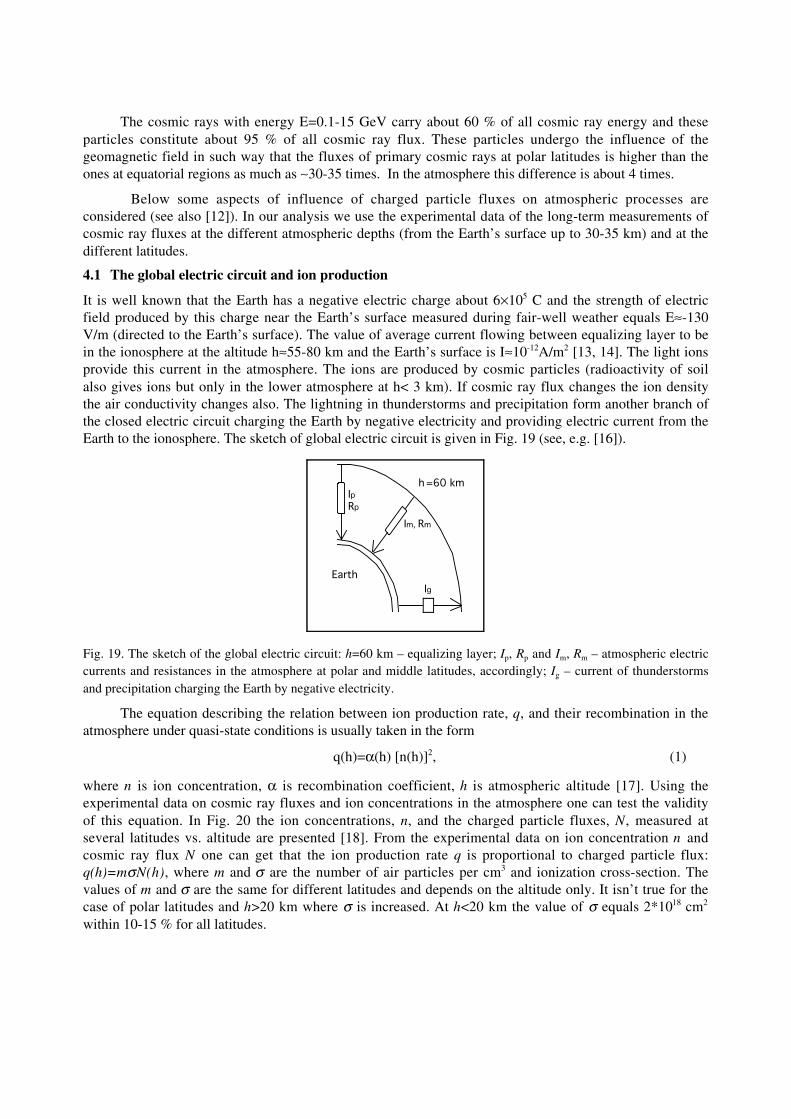
The cosmic rays with energy E=0.1-15 GeV carry about 60 % of all cosmic ray energy and theseparticles constitute about 95 % of all cosmic ray flux. These particles undergo the influence of thegeomagnetic field in such way that the fluxes of primary cosmic rays at polar latitudes is higher than theones at equatorial regions as much as ~30-35 times. In the atmosphere this difference is about 4 times.

Below some aspects of influence of charged particle fluxes on atmospheric processes areconsidered (see also [12]). In our analysis we use the experimental data of the long-term measurements ofcosmic ray fluxes at the different atmospheric depths (from the Earth’s surface up to 30-35 km) and at thedifferent latitudes.

4.1 The global electric circuit and ion production

It is well known that the Earth has a negative electric charge about 6¥105 C and the strength of electricfield produced by this charge near the Earth’s surface measured during fair-well weather equals Eª-130V/m (directed to the Earth’s surface). The value of average current flowing between equalizing layer to bein the ionosphere at the altitude hª55-80 km and the Earth’s surface is Iª10-12A/m2 [13, 14]. The light ionsprovide this current in the atmosphere. The ions are produced by cosmic particles (radioactivity of soilalso gives ions but only in the lower atmosphere at h< 3 km). If cosmic ray flux changes the ion densitythe air conductivity changes also. The lightning in thunderstorms and precipitation form another branch ofthe closed electric circuit charging the Earth by negative electricity and providing electric current from theEarth to the ionosphere. The sketch of global electric circuit is given in Fig. 19 (see, e.g. [16]).

Earth

h =60 kmIpRp

Ig

Im, Rm

Fig. 19. The sketch of the global electric circuit: h=60 km – equalizing layer; Ip, Rp and Im, Rm – atmospheric electriccurrents and resistances in the atmosphere at polar and middle latitudes, accordingly; Ig – current of thunderstormsand precipitation charging the Earth by negative electricity.

The equation describing the relation between ion production rate, q, and their recombination in theatmosphere under quasi-state conditions is usually taken in the form

q(h)=a(h) [n(h)]2, (1)

where n is ion concentration, a is recombination coefficient, h is atmospheric altitude [17]. Using theexperimental data on cosmic ray fluxes and ion concentrations in the atmosphere one can test the validityof this equation. In Fig. 20 the ion concentrations, n, and the charged particle fluxes, N, measured atseveral latitudes vs. altitude are presented [18]. From the experimental data on ion concentration n andcosmic ray flux N one can get that the ion production rate q is proportional to charged particle flux:q(h)=msN(h), where m and s are the number of air particles per cm3 and ionization cross-section. Thevalues of m and s are the same for different latitudes and depends on the altitude only. It isn’t true for thecase of polar latitudes and h>20 km where s is increased. At h<20 km the value of s equals 2*1018 cm2

within 10-15 % for all latitudes.

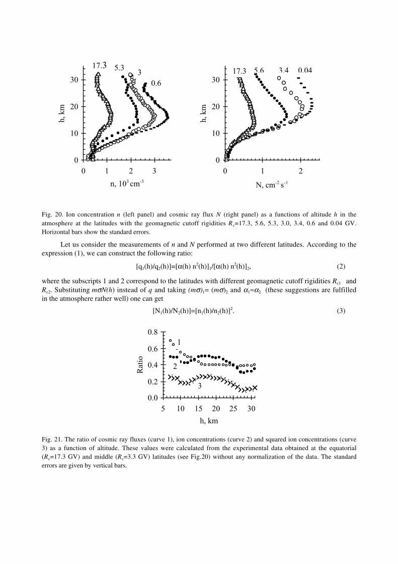
0

10

20

30

0 1 2 3

n, 103 cm-3

h, k

m17.3 5.3

30.6

0

10

20

30

0 1 2

N, cm-2 s-1

h, k

m

17.3 5.6 3.4 0.04

Fig. 20. Ion concentration n (left panel) and cosmic ray flux N (right panel) as a functions of altitude h in theatmosphere at the latitudes with the geomagnetic cutoff rigidities Rc=17.3, 5.6, 5.3, 3.0, 3.4, 0.6 and 0.04 GV.Horizontal bars show the standard errors.

Let us consider the measurements of n and N performed at two different latitudes. According to theexpression (1), we can construct the following ratio:

[q1(h)/q2(h)]=[a(h) n2(h)]1/[a(h) n2(h)]2, (2)

where the subscripts 1 and 2 correspond to the latitudes with different geomagnetic cutoff rigidities Rc1 andRc2. Substituting msN(h) instead of q and taking (ms)1= (ms)2 and a1ªa2 (these suggestions are fulfilledin the atmosphere rather well) one can get

[N1(h)/N2(h)]=[n1(h)/n2(h)]2. (3)

0.0

0.2

0.4

0.6

0.8

5 10 15 20 25 30

h, km

Rat

io

1

2

3

Fig. 21. The ratio of cosmic ray fluxes (curve 1), ion concentrations (curve 2) and squared ion concentrations (curve3) as a function of altitude. These values were calculated from the experimental data obtained at the equatorial(Rc=17.3 GV) and middle (Rc=3.3 GV) latitudes (see Fig.20) without any normalization of the data. The standarderrors are given by vertical bars.

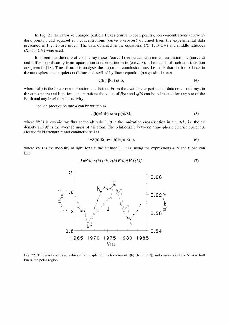
In Fig. 21 the ratios of charged particle fluxes (curve 1-open points), ion concentrations (curve 2-dark points), and squared ion concentrations (curve 3-crosses) obtained from the experimental datapresented in Fig. 20 are given. The data obtained in the equatorial (Rc=17.3 GV) and middle latitudes(Rc=3.3 GV) were used.

It is seen that the ratio of cosmic ray fluxes (curve 1) coincides with ion concentration one (curve 2)and differs significantly from squared ion concentration ratio (curve 3). The details of such considerationare given in [18]. Thus, from this analysis the important conclusion must be made that the ion balance inthe atmosphere under quiet conditions is described by linear equation (not quadratic one)

q(h)=b(h) n(h), (4)

where b(h) is the linear recombination coefficient. From the available experimental data on cosmic rays inthe atmosphere and light ion concentrations the value of b(h) and q(h) can be calculated for any site of theEarth and any level of solar activity.

The ion production rate q can be written as

q(h)=N(h) s(h) r(h)/M, (5)

where N(h) is cosmic ray flux at the altitude h, s is the ionization cross-section in air, r(h) is the airdensity and M is the average mass of air atom. The relationship between atmospheric electric current J,electric field strength E and conductivity l is

J=l(h) E(h)=n(h) k(h) E(h), (6)

where k(h) is the mobility of light ions at the altitude h. Thus, using the expressions 4, 5 and 6 one canfind

J=N(h) s(h) r(h) k(h) E(h)/[M b(h)]. (7)

0.8

1.2

1.6

2

1 9 6 5 1 9 7 0 1 9 7 5 1 9 8 0 1 9 8 5Year

J, 1

0-12 A

m-2

0.54

0.58

0.62

0.66

N, c

m-2

s-1

J

N

Fig. 22. The yearly average values of atmospheric electric current J(h) (from [19]) and cosmic ray flux N(h) at hª8km in the polar region.

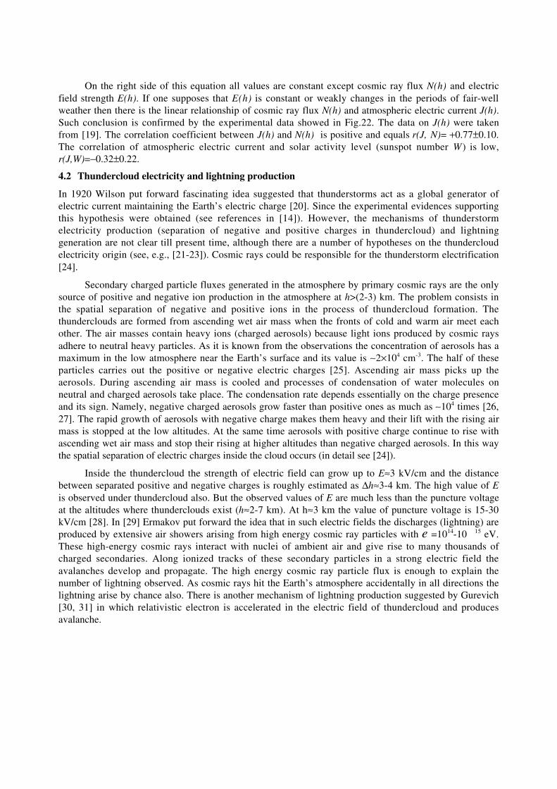
On the right side of this equation all values are constant except cosmic ray flux N(h) and electricfield strength E(h). If one supposes that E(h) is constant or weakly changes in the periods of fair-wellweather then there is the linear relationship of cosmic ray flux N(h) and atmospheric electric current J(h).Such conclusion is confirmed by the experimental data showed in Fig.22. The data on J(h) were takenfrom [19]. The correlation coefficient between J(h) and N(h) is positive and equals r(J, N)= +0.77±0.10.The correlation of atmospheric electric current and solar activity level (sunspot number W) is low,r(J,W)=-0.32±0.22.

4.2 Thundercloud electricity and lightning production

In 1920 Wilson put forward fascinating idea suggested that thunderstorms act as a global generator ofelectric current maintaining the Earth’s electric charge [20]. Since the experimental evidences supportingthis hypothesis were obtained (see references in [14]). However, the mechanisms of thunderstormelectricity production (separation of negative and positive charges in thundercloud) and lightninggeneration are not clear till present time, although there are a number of hypotheses on the thundercloudelectricity origin (see, e.g., [21-23]). Cosmic rays could be responsible for the thunderstorm electrification[24].

Secondary charged particle fluxes generated in the atmosphere by primary cosmic rays are the onlysource of positive and negative ion production in the atmosphere at h>(2-3) km. The problem consists inthe spatial separation of negative and positive ions in the process of thundercloud formation. Thethunderclouds are formed from ascending wet air mass when the fronts of cold and warm air meet eachother. The air masses contain heavy ions (charged aerosols) because light ions produced by cosmic raysadhere to neutral heavy particles. As it is known from the observations the concentration of aerosols has amaximum in the low atmosphere near the Earth’s surface and its value is ~2¥104 cm-3. The half of theseparticles carries out the positive or negative electric charges [25]. Ascending air mass picks up theaerosols. During ascending air mass is cooled and processes of condensation of water molecules onneutral and charged aerosols take place. The condensation rate depends essentially on the charge presenceand its sign. Namely, negative charged aerosols grow faster than positive ones as much as ~104 times [26,27]. The rapid growth of aerosols with negative charge makes them heavy and their lift with the rising airmass is stopped at the low altitudes. At the same time aerosols with positive charge continue to rise withascending wet air mass and stop their rising at higher altitudes than negative charged aerosols. In this waythe spatial separation of electric charges inside the cloud occurs (in detail see [24]).

Inside the thundercloud the strength of electric field can grow up to Eª3 kV/cm and the distancebetween separated positive and negative charges is roughly estimated as Dhª3-4 km. The high value of Eis observed under thundercloud also. But the observed values of E are much less than the puncture voltageat the altitudes where thunderclouds exist (hª2-7 km). At hª3 km the value of puncture voltage is 15-30kV/cm [28]. In [29] Ermakov put forward the idea that in such electric fields the discharges (lightning) areproduced by extensive air showers arising from high energy cosmic ray particles with e =1014-10 15 eV.These high-energy cosmic rays interact with nuclei of ambient air and give rise to many thousands ofcharged secondaries. Along ionized tracks of these secondary particles in a strong electric field theavalanches develop and propagate. The high energy cosmic ray particle flux is enough to explain thenumber of lightning observed. As cosmic rays hit the Earth’s atmosphere accidentally in all directions thelightning arise by chance also. There is another mechanism of lightning production suggested by Gurevich[30, 31] in which relativistic electron is accelerated in the electric field of thundercloud and producesavalanche.

In the process of thundercloud formation one can recognize initial, maturity and decay phases. InFig. 23 these phases and the processes of thundercloud electricity and lightning production are shownschematically [24].

_ _ _ _ _ _ _ _ _ _ _ _ _ _

_ _ _ _ _ __ _ _ _ _ _

+ + + + + ++ + + + +

+ + + + + +

_ _ _ _ _

+ + + +

+

_

1 12 2

3 3

+ + + + + + + + + + +

+ + + + + + ++ + + + + +

+ + + + + ++ + + +

+ _+_+

_ + ++

++

__+_

+ + + + +_ _ _ _ _ __ _ _ _ _

9

a b c87

55

4 _ _ _ _ _ __ _ _ _ _

10

6

J_

+ + + + + _ _ _ _ _

Fig. 23. The phases of thundercloud formation: a – initial phase; b – maturity phase; c – decay phase. Notations: 1and 2 – warm and cold fronts of air; 3-ascending flux of wet air with ions; 4 and 5 – extensive air showers producedby primaries with energies e ≥1014 eV and e ≥ 1015 eV accordingly; 6 – intracloud lightning; 7 – cloud-to-groundlightning; 8 – ground-to-cloud lightning; 9 – the negative screen layer; 10 – positive charge on the cloud base; J –current of negative ions from the ionosphere to the top of the thundercloud.

4.3 The relationship between cosmic rays and other atmospheric phenomena

There are several publications in which the changes of cosmic ray fluxes are considered to be responsiblefor some processes in the atmosphere. Some of such phenomena are listed by Tinsley [16]. Below weanalyze the relationships of cosmic ray fluxes with cloudiness, precipitation and lightning.

The influence of charged particle fluxes on cloudiness was found by Veretenenko and Pudovkin[32]. They found that the value of cloudiness reduced when cosmic ray fluxes in the interplanetary spaceand in the atmosphere decreased during so-called Forbush-effects of cosmic rays. As was shown byStozhkov et al. [33, 34] during Forbush-effects the value of precipitation decreased also. In contrast, whenthe ionization level is increased due to the invasion of solar flare protons into the atmosphere theprecipitation level also increased.

These results were obtained from the analyses of the precipitation data recorded at the numerousmeteorological stations located in Brazil and the Former Soviet Union. More than two hundreds ofForbush-effects and several tens of solar flare events were analyzed. In the analyses the superposed epochmethod was applied. Figures 24 and 25 demonstrate the changes of precipitation in the cases of decreasesand increases of cosmic ray fluxes in the atmosphere [33, 34].

The value of precipitation level decrease obtained by superposed-epoch method for more than 70events of Forbush effects is D0= -(17.4±2.7) %. The probability of the occasional appearance of effect isless than 10-4 if the values of D have a normal distribution. The results on relative increase of rainfall levelof D during solar proton events were obtained by superposed-epoch method for more than 53 events of

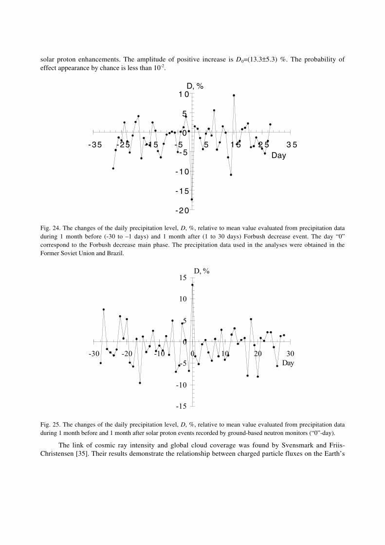
solar proton enhancements. The amplitude of positive increase is D0=(13.3±5.3) %. The probability ofeffect appearance by chance is less than 10-2.

-20

-15

-10

-5

0

5

1 0

-35 -25 -15 -5 5 1 5 2 5 3 5

D, %

Days

Fig. 24. The changes of the daily precipitation level, D, %, relative to mean value evaluated from precipitation dataduring 1 month before (-30 to –1 days) and 1 month after (1 to 30 days) Forbush decrease event. The day “0”correspond to the Forbush decrease main phase. The precipitation data used in the analyses were obtained in theFormer Soviet Union and Brazil.

-15

-10

-5

0

5

10

15

-30 -20 -10 0 10 20 30Day

D, %

Fig. 25. The changes of the daily precipitation level, D, %, relative to mean value evaluated from precipitation dataduring 1 month before and 1 month after solar proton events recorded by ground-based neutron monitors (“0”-day).

The link of cosmic ray intensity and global cloud coverage was found by Svensmark and Friis-Christensen [35]. Their results demonstrate the relationship between charged particle fluxes on the Earth’s

surface and cloudiness during long-term cosmic ray modulation in the 11-year solar activity cycle. Whencosmic ray flux increases cloudiness increases and one can expect that the number of thundercloud (orthundercloud coverage) will increase also. The ion production rate and ion concentration in air grow; thetotal electric charge in the thunderclouds increases. Thus, the number of lightning has to grow and therelationship between cosmic ray flux or ion production rate and thundercloud discharge number has totake place. Now there are the long-term experimental data on lightning flashes over the United States [36]and the link of lightning number and cosmic ray fluxes can be checked. In Fig. 26 the relationship oflightning number L with ion production rate q is shown. The correlation coefficient between these valuesis r(L, q)=+0.85±0.09. The values of q were calculated from the data on cosmic ray flux measured in theatmosphere at the middle latitudes.

10

15

20

25

30

1988 1992 1996 2000

Year

L, 1

06 e

ven

ts/y

ea

r

8

9

10

11

12

q, 1

06 ion

pai

rs/(

cm2 s

)

L

q

Fig. 26. The yearly number of lightning L detected in United States in 1989-1998 (black points, from [36]) and ionproduction rate q in the air column (h=2-10 km) of the middle latitudes (open points).

4.4 Artificial influence on precipitation

The results obtained by Veretenenko and Pudovkin [32], Stozhkov et al. [33], Svensmark and Friis-Christensen [35], Ermakov and Stozhkov [24] show clearly the important role of charged particle fluxeson the cloud, thundercloud formation, and precipitation processes. In the lower atmosphere the changes ofcosmic ray flux during Forbush effects (decrease of cosmic ray flux) or solar proton events (increase offlux) is about (2-15) %. In the first case the decrease of precipitation level is observed, in the second onethe growth of precipitation takes place (see Figs. 24 and 25).

It is possible to increase the flux of charged particles in the lower atmosphere using an electronaccelerator onboard airplane. The accelerated electrons can irradiate the cloud increasing ionization levelinside the cloud. In turn, it could increase precipitation. The modern linear machines accelerating electronsup to the energy of several tens of MeV have a suitable weight and the energy consumption to be installedonboard airplane, e.g. a machine accelerating electrons up to energy 10 MeV with the current 10 mA hasthe weight about 1 ton, sizes of 3¥0.5¥1 m3 and the energy consumption of ~1 kW.

Let us consider a cloud of 3¥3¥2 km3 in sizes, the top of which is at the altitude ~3 km. The flux ofcosmic ray secondaries (mainly relativistic electrons and muons) falling on the upper surface of suchcloud is ~7¥109 particles/s. The total energy released by these particles inside the cloud to ionize air atomsequals ~4.5¥106 erg/s. In contrast, the total energy released by the accelerated electrons (~6¥1013

electrons/s) is ~109 erg/s. Thus, the accelerator with the parameters given above could increase theionization inside the cloud in 10-100 times in comparison with the natural background produced bycosmic rays.

In comparison with the methods of artificial influence on the clouds used in practice [37, 38] theirradiation of clouds by accelerated particles is safe because the accelerated electrons and their secondarieswill be absorbed in ambient air because of its energy losses. The proposed method could be useful tostruggle with droughts and downpours causing floods.

5. CONCLUSION

We present the main characteristics of cosmic ray population in the atmosphere and its variability. Theexperimental data were obtained from the long-term cosmic ray monitoring in the atmosphere from 1957to now. The main features of cosmic ray variability are the following:

• 11-and 22-year solar cycle variations;

• solar proton events originating from powerful solar flares;

• energetic electron precipitation during geomagnetic disturbances and Forbush decreases of cosmicrays;

The cosmic ray monitoring in the atmosphere allows to detect radioactive clouds producing bynuclear explosions or failures at atomic plants.

Cosmic ray particle fluxes play important role in many atmospheric processes and only now thisrole begins to be elucidated. The thundercloud electricity and lightning production, cloud formation,influence on the value of global cloudiness and precipitation on the short (days) and long (11-year solaractivity cycle) time scales, operation of global electric circuit and long-scale global climate changesdepend on the values of cosmic ray flux.

ACKNOWLEDGEMENTS

We are very grateful to our colleagues who made hard work to get the experimental data on the long-termcosmic ray variations in the atmosphere. This work is partly supported by Russian Foundation for BasicResearch (grants No. 01-02-31005 and No. 99-02-18222).

REFERENCES

[1] A.N. Charakhchyan, G.A. Bazilevskaya, Y.I. Stozhkov, and T.N. Charakchyan, Cosmic rays inthe atmosphere and in space near the Earth during 19 and 20 solar activity cycles, Tr. Fis. Inst. imP.N. Lebedeva, Russian Akad. Nauk, Nauka, 83 (1976) 3 (in Russian).

[2] A.E. Golenkov , A.K. Svirzhevskaya, N.S. Svirzhevsky, and Y.I. Stozhkov, Cosmic ray latitudesurvey in the stratosphere during the 1987 solar minimum, Conf. Pap., Int. Cosmic Ray Conf.,XXIst, 7 (1990) 14.

[3] H. Moraal, Observations of the eleven-year cosmic-ray modulation cycle, Space Sci. Rev., 19(1999) 845.

[4] Y.I. Stozhkov and T.N. Charakhchyan, On the role of the heliolatitudes of the sunspots in the 11-year galactic cosmic ray modulation, Acta Physics Academial Sciantiarum Hungaricae, (Suppl.2), 29 (1970).

[5] G.A. Bazilevskaya, M.B. Krainev, Yu.I. Stozhkov , A.K. Svirzhevskay, and N.S. Svirzhevsky,Long-term Soviet program for the measurement of ionizing radiation in the atmosphere, Journ.Geomag. and Geoelectr., 43 (1991) 893.

[6] G.A. Bazilevskaya., A.N. Charakhchyan, Y.I. Stozhkov, and T.N. Charakhchyan, The energyspectrum and the conditions of propagation in the interplanetary space for solar protons during thecosmic ray events on August 4 to 9, 1972, Conf. Pap., Int. Cosmic Ray Conf., XIIIrd, Denver,USA, 2 (1973).

[7] V.S Makhmutov, G.A. Bazilevskaya, A.I. Podgorny, Y.I. Stozhkov, and N.S. Svirzhevsky, Theprecipitation of electrons into the Earth's atmosphere during 1994, Proc. 24 ICRC, Italy, Rome, 4(1995) 1114.

[8] G.A. Bazilevskaya and V.S. Makhmutov, The electron precipitation into the atmosphereaccording to cosmic ray experiment in the stratosphere, Izv. AN SSSR, Ser. Fiz., 63 (1999) 1670(in Russian).

[9] V.S. Makhmutov, G.A. Bazilevskaya, M.B. Krainev, Characteristics of energetic electronrecipitation into the Earth's polar atmosphere and geomagnetic conditions, Adv. Space. Res.,(2001) (in press).

[10] G.D. Reeves, Relativistic electrons and magnetic storms: 1992-1995, Geoph. Res. Lett., 25 (1998)1817.

[11] G.A. Bazilevskaya, A.K. Svirzhevskay, N.S. Svirzhevsky, Y.I. Stozhkov, Radioactive cloud inthe atmosphere at Moscow site on 12-14 April 1993, Kratkie soobsheniya po fizike, Moscow,Lebedev Instituite, 7-8 (1994) 36 (in Russian).

[12] Y.I. Stozhkov, V.I. Ermakov, and P.E. Pokrevsky, Cosmic rays and atmospheric processes, Izv.Russian Akad. Nauk, ser. fiz., 65 (2001) 406 (in Russian).

[13] J. Alan Chalmers, Atmospheric Electricity, Pergamon press (1967).

[14] R. Reiter, Phenomena in Atmosphere and Environmental Electricity, Amsterdam, Elsvier (1992).

[15] R. Markson, Solar modulation of atmospheric electrification and possible implications for theSun-Weather relationship, Nature, 273 (1978) 103.

[16] Brain A. Tinsley, Correlations of atmospheric dynamics with solar wind-induced changes of air-earth current density into cloud tops, Journ. Geophys. Res., 101 (1996) 29,701.

[17] L.B. Loeb, Basic Processes of Gaseous electronics, New-York (1960).

[18] V.I. Ermakov, G.A. Bazilevskaya, P.E. Pokrevsky, and Y.I. Stozhkov. Ion balance equation inthe atmosphere, Journ. Geoph. Res., 102 (1997) 23,413.

[19] R.G. Roble, On solar-terrestrial relationships in the atmospheric electricity, Journ. Geoph. Res.,90 (1985) 6000.

[20] C.T. Wilson, The maintenance of the Earth's electric charge, Observatory, 45 (1922).

[21] E.R. Williams, Electricity of thunderclouds, Scientific American, 1 (1989) 34.

[22] M.B. Baker and J.G. Dash, Mechanism of charge transfer between colliding ice particle inthunderstorms, Journ. Geoph. Res., 99 (1994) 10,621.

[23] V. Brooks, C.P.R. Saunders, An experimental investigation of the inductive mechanism ofthundercloud electrification, Journ. Geoph. Res., 99 (1994) 10,627.

[24] V.I. Ermakov and Y.I. Stozhkov, New mechanism of thundercloud electricity and lightningproduction, Proc. 11-th Intern. Conf. Atmospher. Elect., Alabama, USA (1999) 242.

[25] P.N. Tverscoi, , Course of meteorology, Leningrad, Gidrometeoizdat, (1962) (in Russian).

[26] A.I. Rusanov and V.L. Kusmin, On the influence of electric field on the surface tension of thepolar liquid, Kolloidnyi Journal, 39 (1977) 388 (in Russian).

[27] A.I. Rusanov, To thermodynamics of nucleation on charged centers, Doklady Academii Nauk,USSR, 238 (1978) 831 (in Russian).

[28] J.M. Meek and J. Craggs, Electrical Breakdown of Gases, Oxford, the Claredon Press (1953).

[29] Ermakov , Molnii-sledy chastiz sverchvysokich energii, Nayka I zhizn, Moskva, Prosveshenie(1993) 92 (in Russian).

[30] A.V. Gurevich , G.M. Molikh, and R.A. Roussel-Dupre, Runaway mechanism of air breakdownand preconditioning during a thunderstorm, Phys. Lett., A, 165 (1992) 463.

[31] A.V. Gurevich, K.P. Zubin, R.A. Roussel-Dupre, Lightning initiation by simultaneous effect ofrunaway breakdown and cosmic ray showers, Phys. Lett., A, 254 (1999) 79.

[32] S.V. Veretenenko and M.I. Pudovkin, Effects of forbush-decreases in cloudiness variations,Geomagn. and Aeronomy, 34 (1994) 38 (in Russian).

[33] Y.I. Stozhkov , J. Zullo, Jr., I.M. Martin, G.Q. Pellegrino, H.S. Pinto, P.C. Bezerra, G.A.Bazilevskaya, V.S. Machmutov, N.S. Svirzevskii, A. Turtelli, Jr., Rainfalls during greatForbush-decreases, Nuovo Cimento, 18C (1995) 335.

[34] Y.I. Stozhkov , P.E. Pokrevsky, J. Zullo, Jr., I.M. Martin, V.P. Ohlopkov, G.Q. Pellegrino,H.S. Pinto, P.C. Bezerra, A. Turtelli, Jr., Influence of charged particle fluxes on precipitation,Geomagn. and Aeronomy, 36 (1996) 211 (in Russian).

[35] H. Svensmark and E. Friis-Christensen, Variation of cosmic ray flux and global coverage - amissing link in solar-climate relationships, Journ. Atmospheric and Solar-Terrest. Physics, 59(1997) 1225.

[36] R.E. Orville, G.R. Huffines, Lightning ground flash measurements over contiguous United States:a ten-year summary 1989-1998, Proc. 11th Intern. Conf. Atmospher. Electr., Alabama, USA,(1999) 412.

[37] L.G. Kachurin, Fisicheskie osnovy vosdeistviya na atmosfernye processy, Gidrometeoisdat,Leningrad (1990) (in Russian).

[38] New Scientist, New method of production artificial precipitation, 151 (1996) 10.

CLOUD PROPERTY SURVEY FROM SATELLITE OBSERVATIONSUSING VERTICAL SOUNDERS (TOVS PATH-B) AND IMAGERS(ISCCP)

C. J. Stubenrauch and F. EddouniaLaboratoire de Météorologie Dynamique, Ecole Polytechnique, Palaiseau, France

AbstractSince about 1980 the use of satellite radiometers allows a continuoussurvey of cloud properties over the whole globe. We compare theevolution of cloud amount and effective cloud amount from twodifferent cloud climatologies : ISCCP (International Satellite CloudClimate Project), using imagers onboard geostationary and polar orbitingweather satellites, and TOVS Path-B, obtained from TIROS-N OperationalVertical Sounder (TOVS) measurements onboard polar orbiters. Over aperiod of about ten years (1983-1995), the average cloud amount of about67% and the effective cloud amount of about 53% are quite stable. Themost important disturbance within this period was the volcanic eruption ofMount Pinatubo in June 1991. The slight increase of the visible reflectancesby the volcanic aerosols has led to a slight overestimation of cloud opticalthickness by ISCCP and hence to a slight overestimation of low clouds andunderestimation of the amount of high clouds during the following year.Since infrared radiation is less affected by volcanic aerosols, TOVS cloudproperties should be more reliable. The stable TOVS Path-B effective highcloud amount over the whole period in the tropics indicates that thevolcanic aerosols do not change the properties of high clouds on this scale.

1. CLOUD OBSERVATIONS FROM SATELLITE

Only satellite observations are capable to give a continuous survey of the state of the atmosphere overthe whole globe. At present, twenty years of these measured radiances are available. In order toconvert these radiances into cloud properties, complex inversion algorithms are necessary. Thesealgorithms consist of two parts :

i) cloud detection and

ii) determination of cloud properties using radiative transfer models.

In the following we present two global cloud climatologies. Whereas ISCCP is the cloudclimatology with the best diurnal sampling and spatial resolution, TOVS Path-B cirrus (semi-transparent ice cloud) properties, obtained from vertical sounders with a relatively high spectralresolution, are especially reliable, day and night. However, one has to keep in mind that bothclimatologies give information only on the uppermost cloud.

For climate studies, using one of these datasets, it is important to understand how cloudproperties are perceived by these different instruments and inversion methods. A detailedcomparison has shown that both datasets agree quite well [1]. Discrepancies can be explained bydifferences in temperature profiles, horizontal (partial cloud cover) and vertical (multi-layer clouds)heterogeneities. For example, in the case of thin cirrus overlying low clouds, one determines withTOVS the cirrus properties, whereas ISCCP determines a mixture of both clouds, from the visiblechannel.

1.1 ISCCP climatology

For its global cloud climatology, the International Satellite Cloud Climatology Project (ISCCP) [2,3]puts emphasis on temporal and spatial resolution, rather than on spectral resolution, by using onevisible (VIS, day only) and one infrared (IR) atmospheric window radiance measurement fromimagers on the suite of geostationary and polar orbiting weather satellites. Time sampling is threehourly and the initial spatial resolution of about 5 km is sampled to intervals of about 30 km, whichmeans that about one pixel out of 36 is kept for cloud information. The first ISCCP dataset has beenthoroughly studied (e. g. [4]-[9]). Some of these studies have led to a recent re-analysis [3], mostlyimproving the treatment of cirrus and polar clouds. ISCCP has reprocessed eleven years of data (D-series) from 1983 until 1993. The processing has just taken up again; by the time of writing dataare available until 1997, and the whole data period should be available within the next months.

Clouds are detected through a variable IR-VIS threshold test which compares the measuredradiances to ‘ clear sky composite’ radiances that have been inferred from a series of statistical testson the space and time variations of the IR and VIS radiances [10]. These clear sky conditions areassociated with low IR and VIS spatial and temporal variability.

ISCCP cloud properties are determined for each pixel by comparing the observed radianceswith a detailed radiative transfer model. The model includes the effects of the atmosphere, withproperties specified from the operational analysis of the TOVS data (only one profile per day isavailable), and surface determined from the clear radiances. Cloudy pixels are assumed to be coveredcompletely by a single homogeneous cloud layer. Cloud-top temperature, Tcld, is first retrievedassuming that all clouds are black bodies. During daytime, when VIS radiances are available toretrieve cloud optical thicknesses, t, the cloud-top temperature of ‘ transmissive’ clouds (t < 11) iscorrected to account for the radiation transmitted from below. This means that Tcld is decreased as afunction of t. In the first version of the ISCCP data (C-series), all clouds were represented in theradiative model by a cloud composed of 10 mm radius spherical liquid water droplets; in the newISCCP dataset (D-series), clouds with Tcld ≥ 260 K are treated with the same liquid cloud model, butall clouds with Tcld < 260 K are treated with a model cloud composed of 30 mm ice polycrystals [3].Tcld is converted into cloud-top pressure, pcld, using the operational TOVS atmospheric profiles.Clouds can be classified according to three pcld intervals (separated at 440 and 680 hPa). Duringdaytime, clouds are classified into nine types, by separating each of the three cloud height categoriesinto thin, medium and thick clouds according to three t intervals (divided at 3.6 and 23).

Among many other variables, the D2 dataset gives statistics on cloud amount, CA, as calculatedin Equation (1), and cloud amount separately for high, midlevel and lowlevel clouds at a spatialresolution of 2.5∞.

CA = Ncld / Ntot. (1)

where Ncld is the number of cloudy pixels within the grid, and

Ntot is the total number of pixels within the grid.

1.2 TOVS Path-B climatology

The Improved Initialization Inversion (3I) algorithms [11] convert infrared and microwave radiationmeasured from the TIROS-N Operational Vertical Sounder (TOVS) onboard the NOAA polarorbiters into atmospheric temperature and humidity profiles and into cloud and surface properties.Within the framework of the NOAA/NASA Pathfinder Program, eight years of TOVS data (1987-1995) have already been processed at LMD. This TOVS Path-B dataset provides theseatmospheric parameters at a spatial resolution of 1∞ [12]. Results for the whole TOVS observationperiod from 1979 until now should be available by the end of 2001, since the re-calibration of theHIRS brightness temperatures obtained by comparing airmass-averaged brightness temperatures

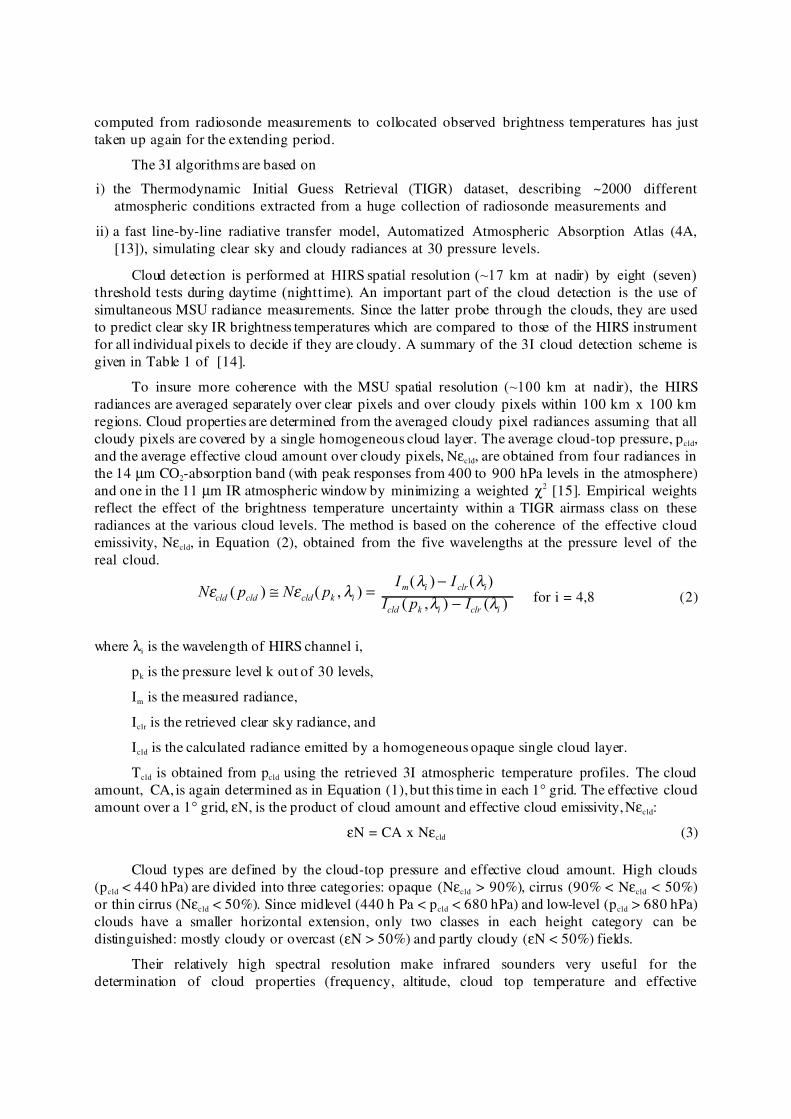
computed from radiosonde measurements to collocated observed brightness temperatures has justtaken up again for the extending period.

The 3I algorithms are based on

i) the Thermodynamic Initial Guess Retrieval (TIGR) dataset, describing ~2000 differentatmospheric conditions extracted from a huge collection of radiosonde measurements and

ii) a fast line-by-line radiative transfer model, Automatized Atmospheric Absorption Atlas (4A,[13]), simulating clear sky and cloudy radiances at 30 pressure levels.

Cloud detection is performed at HIRS spatial resolution (~17 km at nadir) by eight (seven)threshold tests during daytime (nighttime). An important part of the cloud detection is the use ofsimultaneous MSU radiance measurements. Since the latter probe through the clouds, they are usedto predict clear sky IR brightness temperatures which are compared to those of the HIRS instrumentfor all individual pixels to decide if they are cloudy. A summary of the 3I cloud detection scheme isgiven in Table 1 of [14].

To insure more coherence with the MSU spatial resolution (~100 km at nadir), the HIRSradiances are averaged separately over clear pixels and over cloudy pixels within 100 km x 100 kmregions. Cloud properties are determined from the averaged cloudy pixel radiances assuming that allcloudy pixels are covered by a single homogeneous cloud layer. The average cloud-top pressure, pcld,and the average effective cloud amount over cloudy pixels, Necld, are obtained from four radiances inthe 14 mm CO2-absorption band (with peak responses from 400 to 900 hPa levels in the atmosphere)and one in the 11 mm IR atmospheric window by minimizing a weighted c2 [15]. Empirical weightsreflect the effect of the brightness temperature uncertainty within a TIGR airmass class on theseradiances at the various cloud levels. The method is based on the coherence of the effective cloudemissivity, Necld, in Equation (2), obtained from the five wavelengths at the pressure level of thereal cloud.

N p N pI I

I p Icld cld cld k im i clr i

cld k i clr i

e e ll ll l

( ) ( , )( ) ( )

( , ) ( )@ =

-- for i = 4,8 (2)

where li is the wavelength of HIRS channel i,

pk is the pressure level k out of 30 levels,

Im is the measured radiance,

Iclr is the retrieved clear sky radiance, and

Icld is the calculated radiance emitted by a homogeneous opaque single cloud layer.

Tcld is obtained from pcld using the retrieved 3I atmospheric temperature profiles. The cloudamount, CA, is again determined as in Equation (1), but this time in each 1∞ grid. The effective cloudamount over a 1∞ grid, eN, is the product of cloud amount and effective cloud emissivity, Necld:

eN = CA x Necld (3)

Cloud types are defined by the cloud-top pressure and effective cloud amount. High clouds(pcld < 440 hPa) are divided into three categories: opaque (Necld > 90%), cirrus (90% < Necld < 50%)or thin cirrus (Necld < 50%). Since midlevel (440 h Pa < pcld < 680 hPa) and low-level (pcld > 680 hPa)clouds have a smaller horizontal extension, only two classes in each height category can bedistinguished: mostly cloudy or overcast (eN > 50%) and partly cloudy (eN < 50%) fields.

Their relatively high spectral resolution make infrared sounders very useful for thedetermination of cloud properties (frequency, altitude, cloud top temperature and effective

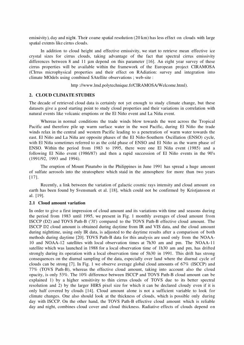
emissivity), day and night. Their coarse spatial resolution (20 km) has less effect on clouds with largespatial extents like cirrus clouds.

In addition to cloud height and effective emissivity, we start to retrieve mean effective icecrystal sizes for cirrus clouds, taking advantage of the fact that spectral cirrus emissivitydifferences between 8 and 11 mm depend on this parameter [16]. An eight year survey of thesecirrus properties will be available within the framework of the European project CIRAMOSA(CIrrus microphysical properties and their effect on RAdiation: survey and integration intoclimate MOdels using combined SAtellite observations ; web-site :

http ://www.lmd.polytechnique.fr/CIRAMOSA/Welcome.html).

2. CLOUD CLIMATE STUDIES

The decade of retrieved cloud data is certainly not yet enough to study climate change, but thesedatasets give a good starting point to study cloud properties and their variations in correlation withnatural events like volcanic eruptions or the El Niño event and La Niña event.

Whereas in normal conditions the trade winds blow towards the west across the TropicalPacific and therefore pile up warm surface water in the west Pacific, during El Niño the tradewinds relax in the central and western Pacific leading to a penetration of warm water towards theeast. El Niño and La Niña are opposite phases of the El Niño-Southern Oscillation (ENSO) cycle,with El Niña sometimes referred to as the cold phase of ENSO and El Niño as the warm phase ofENSO. Within the period from 1983 to 1995, there were one El Niña event (1985) and afollowing El Niño event (1986/87) and then a rapid succession of El Niño events in the 90's(1991/92, 1993 and 1994).

The eruption of Mount Pinatubo in the Philippines in June 1991 has spread a huge amountof sulfate aerosols into the stratosphere which staid in the atmosphere for more than two years[17].

Recently, a link between the variation of galactic cosmic rays intensity and cloud amount onearth has been found by Svensmark et al. [18], which could not be confirmed by Kristjansson etal. [19].

2.1 Cloud amount variation

In order to give a first impression of cloud amount and its variations with time and seasons duringthe period from 1983 until 1995, we present in Fig. 1 monthly averages of cloud amount fromISCCP (D2) and TOVS Path-B ('3I') compared to the TOVS Path-B effective cloud amount. TheISCCP D2 cloud amount is obtained during daytime from IR and VIS data, and the cloud amountduring nighttime, using only IR data, is adjusted to the daytime results after a comparison of bothmethods during daytime [20]. TOVS Path-B data for this analysis are used only from the NOAA-10 and NOAA-12 satellites with local observation times at 7h30 am and pm. The NOAA-11satellite which was launched in 1988 for a local observation time of 1h30 am and pm, has driftedstrongly during its operation with a local observation time of 5h30 in 1991. This drift has strongconsequences on the diurnal sampling of the data, especially over land where the diurnal cycle ofclouds can be strong [7]. In Fig. 1 we observe average global cloud amounts of 67% (ISCCP) and77% (TOVS Path-B), whereas the effective cloud amount, taking into account also the cloudopacity, is only 53%. The 10% difference between ISCCP and TOVS Path-B cloud amount can beexplained 1) by a higher sensitivity to thin cirrus clouds of TOVS due to its better spectralresolution and 2) by the larger HIRS pixel size for which it can be declared cloudy even if it isonly half covered by clouds [14]. Cloud amount alone is not a sufficient variable to look forclimate changes. One also should look at the thickness of clouds, which is possible only duringday with ISCCP. On the other hand, the TOVS Path-B effective cloud amount which is reliableday and night, combines cloud cover and cloud thickness. Radiative effects of clouds depend on

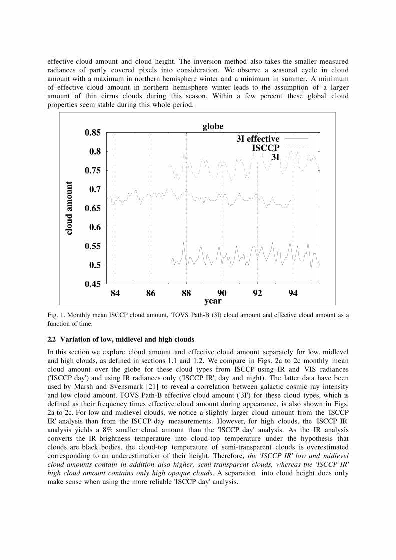
effective cloud amount and cloud height. The inversion method also takes the smaller measuredradiances of partly covered pixels into consideration. We observe a seasonal cycle in cloudamount with a maximum in northern hemisphere winter and a minimum in summer. A minimumof effective cloud amount in northern hemisphere winter leads to the assumption of a largeramount of thin cirrus clouds during this season. Within a few percent these global cloudproperties seem stable during this whole period.

0.45

0.5

0.55

0.6

0.65

0.7

0.75

0.8

0.85

84 86 88 90 92 94

clou

d am

ount

year

globe3I effective

ISCCP3I

Fig. 1. Monthly mean ISCCP cloud amount, TOVS Path-B (3I) cloud amount and effective cloud amount as afunction of time.

2.2 Variation of low, midlevel and high clouds

In this section we explore cloud amount and effective cloud amount separately for low, midleveland high clouds, as defined in sections 1.1 and 1.2. We compare in Figs. 2a to 2c monthly meancloud amount over the globe for these cloud types from ISCCP using IR and VIS radiances('ISCCP day') and using IR radiances only ('ISCCP IR', day and night). The latter data have beenused by Marsh and Svensmark [21] to reveal a correlation between galactic cosmic ray intensityand low cloud amount. TOVS Path-B effective cloud amount ('3I') for these cloud types, which isdefined as their frequency times effective cloud amount during appearance, is also shown in Figs.2a to 2c. For low and midlevel clouds, we notice a slightly larger cloud amount from the 'ISCCPIR' analysis than from the ISCCP day measurements. However, for high clouds, the 'ISCCP IR'analysis yields a 8% smaller cloud amount than the 'ISCCP day' analysis. As the IR analysisconverts the IR brightness temperature into cloud-top temperature under the hypothesis thatclouds are black bodies, the cloud-top temperature of semi-transparent clouds is overestimatedcorresponding to an underestimation of their height. Therefore, the 'ISCCP IR' low and midlevelcloud amounts contain in addition also higher, semi-transparent clouds, whereas the 'ISCCP IR'high cloud amount contains only high opaque clouds. A separation into cloud height does onlymake sense when using the more reliable 'ISCCP day' analysis.

10

15

20

25

30

35

84 86 88 90 92 94

low

clo

ud a

mou

nt

year

globe

3I effectiveISCCP dayISCCP IR

10

15

20

25

30

35

84 86 88 90 92 94

mid

clo

ud a

mou

nt

year

globe3I effectiveISCCP dayISCCP IR

10

15

20

25

30

35

84 86 88 90 92 94

high

clo

ud a

mou

nt

year

globe3I effectiveISCCP dayISCCP IR

Fig. 2. Monthly mean ISCCP cloud amount from VIS and IR radiances (day) and from IR radiances only (IR), aswell as TOVS Path-B (3I) effective cloud amount as a function of time a) for low clouds, b) for midlevel cloudsand c) for high clouds.

The difference between ‘ISCCP day’ cloud amount and TOVS Path-B effective cloudamount should give an estimation of cloud thickness. This difference is negligible for low cloudsin northern hemisphere winter, but 5% for low clouds in northern hemisphere summer. Alsomidlevel clouds and high clouds have in general an about 6% smaller effective cloud amount.This means that on average low clouds are slightly thicker in northern hemisphere winter, andthere is a high occurrence of semi-transparent cirrus clouds over the globe (about 25%, notshown). The slight increase of ‘ISCCP day’ low cloud amount and TOVS Path-B effective low

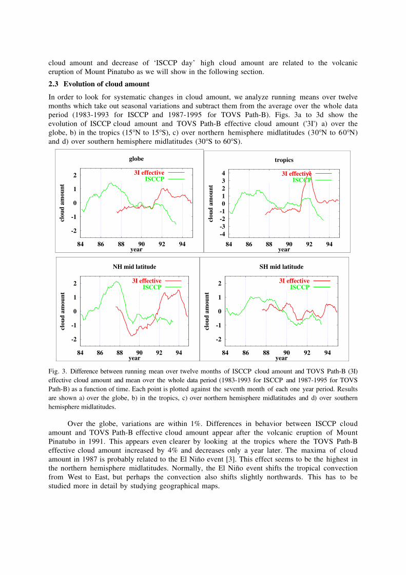
cloud amount and decrease of ‘ISCCP day’ high cloud amount are related to the volcaniceruption of Mount Pinatubo as we will show in the following section.

2.3 Evolution of cloud amount

In order to look for systematic changes in cloud amount, we analyze running means over twelvemonths which take out seasonal variations and subtract them from the average over the whole dataperiod (1983-1993 for ISCCP and 1987-1995 for TOVS Path-B). Figs. 3a to 3d show theevolution of ISCCP cloud amount and TOVS Path-B effective cloud amount ('3I') a) over theglobe, b) in the tropics (15∞N to 15∞S), c) over northern hemisphere midlatitudes (30∞N to 60∞N)and d) over southern hemisphere midlatitudes (30∞S to 60∞S).

-2

-1

0

1

2

84 86 88 90 92 94

clou

d am

ount

year

globe

3I effectiveISCCP

-4-3-2-101234

84 86 88 90 92 94

clou

d am

ount

year

tropics

3I effectiveISCCP

-2

-1

0

1

2

84 86 88 90 92 94

clou

d a

mou

nt

year

NH mid latitude

3I effectiveISCCP

-2

-1

0

1

2

84 86 88 90 92 94

clou

d am

ount

year

SH mid latitude

3I effectiveISCCP

Fig. 3. Difference between running mean over twelve months of ISCCP cloud amount and TOVS Path-B (3I)effective cloud amount and mean over the whole data period (1983-1993 for ISCCP and 1987-1995 for TOVSPath-B) as a function of time. Each point is plotted against the seventh month of each one year period. Resultsare shown a) over the globe, b) in the tropics, c) over northern hemisphere midlatitudes and d) over southernhemisphere midlatitudes.

Over the globe, variations are within 1%. Differences in behavior between ISCCP cloudamount and TOVS Path-B effective cloud amount appear after the volcanic eruption of MountPinatubo in 1991. This appears even clearer by looking at the tropics where the TOVS Path-Beffective cloud amount increased by 4% and decreases only a year later. The maxima of cloudamount in 1987 is probably related to the El Niño event [3]. This effect seems to be the highest inthe northern hemisphere midlatitudes. Normally, the El Niño event shifts the tropical convectionfrom West to East, but perhaps the convection also shifts slightly northwards. This has to bestudied more in detail by studying geographical maps.

2.4 Evolution of high and low clouds

If one wants to study correlations between cloud amount and the variation of galactic cosmic rayintensity, one should look for them at high clouds and at higher latitudes, since the intensitydecreases by entering the atmosphere and since the Earth magnetic field is lower at these latitudes.Figs. 4a to 4d shows the evolution of ISCCP high cloud amount from ISCCP using IR and VISradiances ('ISCCP day') and using only IR radiances ('ISCCP IR', day and night) and of TOVSPath-B effective high cloud amount ('3I') a) over the globe, b) in the tropics, c) over northernhemisphere midlatitudes and d) over southern hemisphere midlatitudes.

-3

-2

-1

0

1

2

3

84 86 88 90 92 94

high

clo

ud a

mou

nt

year

globe

3I effectiveISCCP IR

ISCCP day

-4-3-2-101234

84 86 88 90 92 94

high

clo

ud a

mou

nt

year

tropics

3I effectiveISCCP IR

ISCCP day

-3

-2

-1

0

1

2

3

84 86 88 90 92 94

high

clo

ud a

mou

nt

year

NH mid latitude

3I effectiveISCCP IR

ISCCP day

-3

-2

-1

0

1

2

3

84 86 88 90 92 94

high

clo

ud a

mou

nt

year

SH mid latitude

3I effectiveISCCP IR

ISCCP day

Fig. 4. Difference between running mean over twelve months of ISCCP high cloud amount from VIS and IRradiances (day) and from IR radiances only (IR), as well as TOVS Path-B (3I) effective high cloud amount andmean over the whole corresponding data period as a function of time. Each point is plotted against the seventhmonth of each one year period. Results are shown a) over the globe, b) in the tropics, c) over northernhemisphere midlatitudes and d) over southern hemisphere midlatitudes.

From these figures we conclude that there are no significant variations of the effective highcloud amount and of the 'ISCCP IR' high cloud amount, corresponding to high opaque cloudsonly. However, the 'ISCCP day' high cloud amount decreases by 2.5% globally and 4% in thetropics after the volcanic eruption of Mount Pinatubo in 1991. This effect can be explained bythe increase of the VIS reflectance by the volcanic aerosols of this eruption which have had anoptical thickness of more than 0.1. In the ISCCP cloud property retrieval this increase in VISreflectance affects then the optical thickness of the clouds, and an overestimation of opticalthickness leads then to an underestimation of cloud height [3].

This can be seen in Figs. 5a and 5b which show the evolution ISCCP low cloud amountfrom ISCCP using IR and VIS radiances ('ISCCP day') and using only IR radiances and of TOVSPath-B effective low cloud amount ('3I') a) over the globe and b) in the tropics. The low cloudamount increase from 'ISCCP day' by 3% in the tropics (and midlevel cloud amount increase by

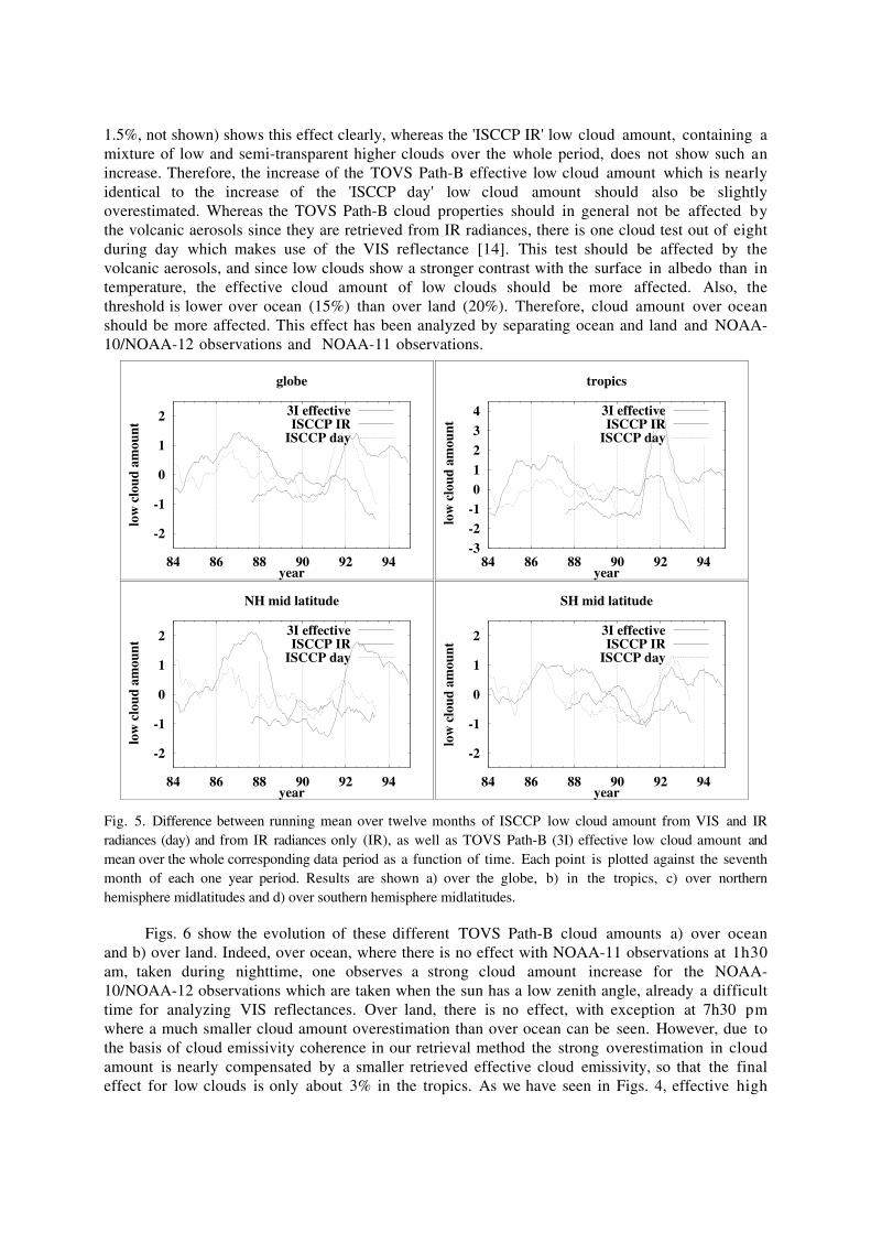
1.5%, not shown) shows this effect clearly, whereas the 'ISCCP IR' low cloud amount, containing amixture of low and semi-transparent higher clouds over the whole period, does not show such anincrease. Therefore, the increase of the TOVS Path-B effective low cloud amount which is nearlyidentical to the increase of the 'ISCCP day' low cloud amount should also be slightlyoverestimated. Whereas the TOVS Path-B cloud properties should in general not be affected bythe volcanic aerosols since they are retrieved from IR radiances, there is one cloud test out of eightduring day which makes use of the VIS reflectance [14]. This test should be affected by thevolcanic aerosols, and since low clouds show a stronger contrast with the surface in albedo than intemperature, the effective cloud amount of low clouds should be more affected. Also, thethreshold is lower over ocean (15%) than over land (20%). Therefore, cloud amount over oceanshould be more affected. This effect has been analyzed by separating ocean and land and NOAA-10/NOAA-12 observations and NOAA-11 observations.

-2

-1

0

1

2

84 86 88 90 92 94

low

clo

ud a

mou

nt

year

globe

3I effectiveISCCP IR

ISCCP day

-3-2

-10

123

4

84 86 88 90 92 94

low

clo

ud a

mou

nt

year

tropics

3I effectiveISCCP IR

ISCCP day

-2

-1

0

1

2

84 86 88 90 92 94

low

clo

ud a

mou

nt

year

NH mid latitude

3I effectiveISCCP IR

ISCCP day

-2

-1

0

1

2

84 86 88 90 92 94

low

clo

ud a

mou

nt

year

SH mid latitude

3I effectiveISCCP IR

ISCCP day

Fig. 5. Difference between running mean over twelve months of ISCCP low cloud amount from VIS and IRradiances (day) and from IR radiances only (IR), as well as TOVS Path-B (3I) effective low cloud amount andmean over the whole corresponding data period as a function of time. Each point is plotted against the seventhmonth of each one year period. Results are shown a) over the globe, b) in the tropics, c) over northernhemisphere midlatitudes and d) over southern hemisphere midlatitudes.

Figs. 6 show the evolution of these different TOVS Path-B cloud amounts a) over oceanand b) over land. Indeed, over ocean, where there is no effect with NOAA-11 observations at 1h30am, taken during nighttime, one observes a strong cloud amount increase for the NOAA-10/NOAA-12 observations which are taken when the sun has a low zenith angle, already a difficulttime for analyzing VIS reflectances. Over land, there is no effect, with exception at 7h30 pmwhere a much smaller cloud amount overestimation than over ocean can be seen. However, due tothe basis of cloud emissivity coherence in our retrieval method the strong overestimation in cloudamount is nearly compensated by a smaller retrieved effective cloud emissivity, so that the finaleffect for low clouds is only about 3% in the tropics. As we have seen in Figs. 4, effective high

cloud amount is not affected by volcanic aerosols. Nevertheless, we will improve this clouddetection test in the next TOVS Path-B re-analysis.

6065707580859095

100

88 89 90 91 92 93 94 95

clou

d am

ount

year

tropical ocean

NOAA1012 am NOAA11 am

NOAA1012 pm NOAA11 pm

6065707580859095

100

88 89 90 91 92 93 94 95

clou

d am

ount

year

tropical land

NOAA1012 am NOAA11 am

NOAA1012 pm NOAA11 pm

Fig. 6. Running mean over TOVS Path-B (3I) cloud amount from different satellite observations as a function oftime. Each point is plotted against the seventh month of each one year period. Results are shown for a) tropicalocean and b) tropical land.

3. CONCLUSION AND OUTLOOK

Satellite observations provide a unique possibility to survey cloud properties over a long period oftime. During the observed decade (1983-1995), the average cloud amount of about 67% andeffective cloud amount of about 53% are stable within 2% over the globe.

Within this period, the most important disturbance was the volcanic eruption of MountPinatubo in the Philippines in June 1991. The volcanic aerosols which had an optical thickness ofmore than 0.1 slightly increased the VIS reflectances. Whereas the ISCCP cloud amount andTOVS Path-B effective high cloud amount were not affected by this event, the 'ISCCP day' highcloud amount is slightly underestimated (4.5% in the tropics and 2.5% over the globe) and the'ISCCP day' low amount overestimated (4% in the tropics and 1% over the globe). Nevertheless, aseparation into cloud height does only make sense when using the more reliable 'ISCCP day'analysis, since the 'ISCCP IR' low and midlevel cloud amounts contain in addition also higher,semi-transparent clouds, whereas the 'ISCCP IR' high cloud amount contains only high opaqueclouds. The TOVS Path-B effective low cloud amount is also slightly overestimated (4% in thetropics and 1% over the globe), because one of the cloud detection tests makes use of the VISreflectance.

As has been pointed out earlier, if there are any correlations between the galactic cosmic rayintensity and cloud properties these should occur for high clouds and at higher latitudes. TheTOVS Path-B effective high cloud amount which is stable within 1% over the whole observationperiod does not show any correlation with the cosmic ray intensity variations. It should be notedthat cloud radiative effects are determined not only by cloud amount but depend also on cloudthickness and effective cloud amount includes both variables.

Both datasets will be extended. By the time of writing, ISCCP data processing has alreadystarted again, and the whole data period (1983 until now) should be available within the nextmonths. TOVS Path-B processing just started with the re-calibration of the HIRS brightnesstemperatures, and the whole TOVS observation period from 1979 until now should be availableby the end of 2001.

ACKNOWLEDGEMENTS

Our thanks to W. B. Rossow for many stimulating discussions within the last years in order toadvance in understanding both cloud datasets. We also want to thank the rest of our ARA

(Analyse du Rayonnement Atmosphérique) group for their support, and especially S. Serrar andR. Armante for their help in computational matters and G. Rädel for bringing our attention toCERN again.

REFERENCES

[1] Stubenrauch, C. J., W. B. Rossow , N. A. Scott, and A. Chédin, Clouds as Seen by SatelliteSounders (3I) and Imagers (ISCCP): III) Spatial Heterogeneity and Radiative Effects,J. Climate 12 (1999) 3419-3442.

[2] W. B. Rossow and R. A. Schiffer, ISCCP Cloud Data Products. Bull. Amer. Meteor. Soc.72 (1991) 1-20.

[3] W. B. Rossow and R. A. Schiffer, Advances in understanding clouds from ISCCP. Bull.Amer. Meteor. Soc. 80 (1999) 2261-2287.

[4] R. Fu, A. D. Del Genio, and W. B. Rossow, Behavior of deep convective clouds in thetropical Pacific deduced from ISCCP radiances. J. Climate 3 (1990) 1129-1152.

[5] G. Tselioudis, W. B. Rossow, and D. Rind, Global patterns of cloud optical thicknessvariation with temperature, J. Climate 5 (1992) 1484-1495.

[6] S. A. Klein and D. L. Hartmann, The seasonal cycle of low stratiform clouds. J. Climate 6(1993) 1587-1606.

[7] B. Cairns, Diurnal variations of cloud from ISCCP data. Atm. Res. 37 (1995) 133-146.

[8] X. Liao, W. B. Rossow and D. Rind,: Comparison between SAGE II and ISCCP High-LevelCloulds. Part II: Locating Cloud Tops. J. Geophys. Res. 100 (1995) 1137-1147.

[9] Y. Jin, W. B. Rossow and D. P. Wylie, Comparison of the Climatologies of High-LevelClouds from HIRS and ISCCP. J. Climate. 9 (1996) 2850-2879.

[10] W. B. Rossow and L. C. Garder, Cloud detection using satellite measurements of infraredand visible radiances for ISCCP. J. Climate 6 (1993) 2341-2369.

[11] A. Chédin, N. A. Scott, C. Wahiche and P. Moulinier, The Improved Initialized Inversionmethod: A high resolution physical method for temperature retrievals from the TIROS-NSeries. J. Clim. Appl. Meteor. 24 (1985) 124-143.

[12] N. A. Scott, A. Chédin, R. Armante, J. Francis, C. J. Stubenrauch, J.-P. Chaboureau, F.Chevallier, C. Claud and F. Chéruy, Characteristics of the TOVS Pathfinder Path-BDataset. Bull. Amer. Meteor. Soc. 80 (1999) 2679-2701.

[13] N. A. Scott, and A. Chédin, A fast line-by-line method for atmospheric absorptioncomputations: The Automized Atmospheric Absorption Atlas. J. Appl. Meteor. 20(1981) 802-812.

[14] C. J. Stubenrauch, W. B. Rossow , F. Chéruy, N. A. Scott and A. Chédin, Clouds as Seenby Satellite Sounders (3I) and Imagers (ISCCP): I) Evaluation of Cloud Parameters, J.Climate 12 (1999) 2189-2213.

[15] C. J. Stubenrauch, A. Chédin, R. Armante and N. A. Scott, Clouds as Seen by SatelliteSounders (3I) and Imagers (ISCCP): II) A New Approach for Cloud ParameterDetermination in the 3I Algorithms, J. Climate 12 (1999) 2214-2223.

[16] C. J. Stubenrauch, R. Holz, A. Chédin, D. Mitchell and A. J. Baran, Retrieval of Cirrus IceCrystal Sizes from 8.3 and 11.1 mm Emissivities Determined by the ImprovedInitialization Inversion of TIROS-N Operational Vertical Sounder Observations, J.Geophys. Res. 104 (1999) 31793-31808.

[17] M. P. McCormick, L. W. Thomason, and C. R. Trepte, Atmospheric effects of the MtPinatubo eruption, Nature 373 (1995) 399-404.

[18] H. Svensmark and E. Friis-Christensen, Variation of cosmic ray flux and global cloudcoverage: A missing link in solar climate relationships, J. Atmos. Sol. Terr. Phys. 59(1997) 1225-1232.

[19] J. E. Kristjansson, and J. Kristiansen, Is there a cosmic ray signal in recent variations inglobal cloudiness and cloud radiative forcing?, J. Geophys. Res. 105 (2000) 11,851-11,863.

[20] W. B. Rossow, A. W. Walker, D. Beuschel, and M. Roiter, International Satellite CloudClimatology Project (ISCCP) description of new cloud datasets, World Climate ResearchProgramme (ICSU and WMO) WMO/TD-No.737 (1996) 115pp.

[21] N. Marsh, and H. Svensmark, Cosmic rays, clouds, and climate, Space Science Reviews 94(2000) 215-230.

ATMOSPHERIC ELECTRICITY AND CLOUD MICROPHYSICS

R. G. HarrisonDepartment of Meteorology, The University of Reading, P.O. Box 243, Reading RG6 6BB, UK

AbstractThe terrestrial atmospheric electrical system covers a range ofdimensional scales, from charged molecular clusters to convective cloudsystems. Charge-exchange associated with thunderclouds leads to positivecharge in the upper conductive regions of the atmosphere and a netnegative charge on the planetary surface. In non-thunderstorm regions, avertical ionic current flows, replenishing the air with molecular ionsotherwise removed by attachment, recombination or nucleationprocesses. Ions may have indirect effects on non-thunderstorm clouds,and therefore conceivably on climate, via cloud microphysical processes.Cloud Condensation Nuclei (CCN) and Ice Nuclei (IN) are necessary forthe formation of water clouds and freezing of ice clouds respectively. Inboth cases, ionisation may be important: it is now known that ultrafineaerosol can be formed from ionisation, probably providing an additionalsource of CCN. It is also known that electrified aerosol, perhaps active asIN, can be collected by droplets more effectively than neutral particles.

1. INTRODUCTION

Electrical processes in atmospheric air arise from the combined effect of natural ionisation andthe natural electric fields generated indirectly by charge separation in thunderclouds. In non-thunderstorm regions, which probably constitute the majority of the global cloud area, theelectrical processes will not generate the large breakdown electric fields associated with lightning,but microscopic aerosol particles acquire charges by diffusion of the molecular cluster ionsformed from ionisation.

In this overview, the effect of small charges on aerosol particles and droplets are considered.Since the charge arises from radiolysis of air by cosmic rays and natural radioactivity, thediscussion here is structured in terms of the processes associated with charge generation andremoval, including tutorial material on microphysical cloud processes. It has been observed(Marsh and Svensmark, 2000) that there is a correlation between low cloud properties and theneutrons produced by cosmic rays.

2. THUNDERSTORMS AND GLOBAL ELECTRIFICATION

The atmospheric electrical system originally discussed by Wilson (1929) can be simplified into anelectric circuit in which thunderstorms separate charge in convective regions. The chargeseparation leads to a potential difference between conductive regions of the upper atmosphere andthe surface, which causes an ionic leakage current to flow vertically (figure 1). Currents of order2000A flow in the circuit, with an upper atmosphere potential of ~300kV. The conduction currentdensity in undisturbed regions is ~2pA.m-2.

The charge-exchange processes within thunderclouds are complicated, and probably resultfrom the interaction between rising ice crystals rising and riming soft hail (graupel). Typicalmicrophysical collisions exchange charge with typical magnitudes of tens of femtoCoulombs, butthe precise magnitude and polarity is greatly influenced by the liquid water content andtemperature (MacGorman and Rust, 1998).

Figure 1. The global atmospheric electrical circuit (from Harrison, 1997).

3. ATMOSPHERIC PROPERTIES AND CLOUD MICROPHYSICS

3.1 Atmospheric properties

3.1.1 Bulk properties

The troposphere (lower atmosphere) shows variations in temperature and water content, andpartitioning of the water concentration between liquid, solid or vapour forms is critical to theformation and distribution of clouds. Figure 2 shows a vertical sounding of temperature andhumidity, which illustrates the atmospheric structure. The presence of low cloud (which wasobserved from the surface) is evident from the sharp increase in relative humidity, marked as A. Bshows a slight temperature inversion associated with the top of the planetary boundary layer, andat C the temperature ceases to fall with height, at the tropopause. It is clear that there isconsiderable variability in the relative humidity during the ascent, and in the region where cloudwas identified optically.

Radiosonde ascent on 22nd March 1998 at 1400h,(launched from Medina Valley, Isle of Wight, UK)

0

200

400

600

800

1000

0 5000 10000 15000 20000

altitude/mpres

sure

/mba

r

-80

-60

-40

-20

0

20

40

60

80

tem

pera

ture

(de

gC)

and

Rel

ativ

e H

umid

ity(%

)

pressure

air temperature

relative humidity

B

A

C

Figure 2. Vertical atmospheric sounding in non-frontal synoptic conditions, showing relative humidity,temperature and pressure variations with height. (A, B and C are discussed in the text.)

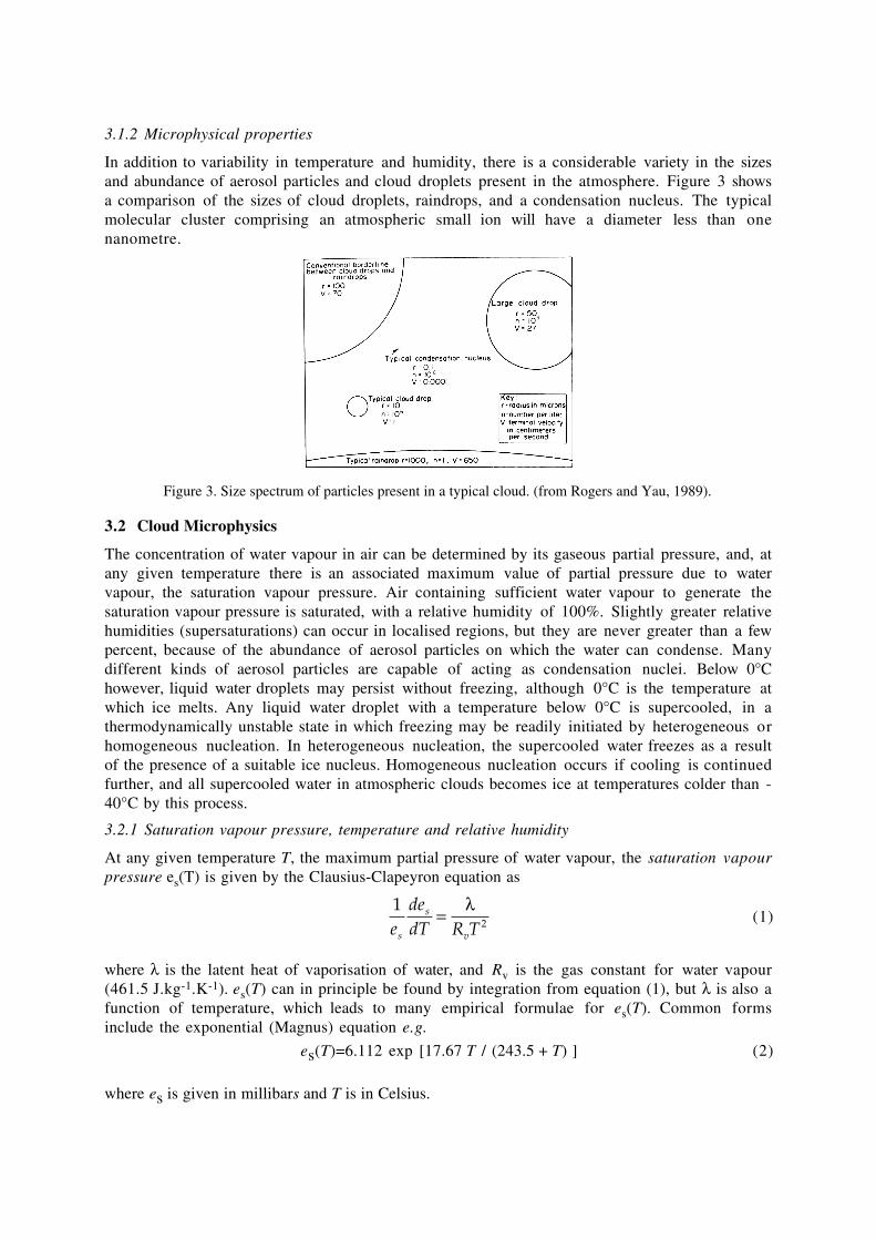
3.1.2 Microphysical properties

In addition to variability in temperature and humidity, there is a considerable variety in the sizesand abundance of aerosol particles and cloud droplets present in the atmosphere. Figure 3 showsa comparison of the sizes of cloud droplets, raindrops, and a condensation nucleus. The typicalmolecular cluster comprising an atmospheric small ion will have a diameter less than onenanometre.

Figure 3. Size spectrum of particles present in a typical cloud. (from Rogers and Yau, 1989).

3.2 Cloud Microphysics

The concentration of water vapour in air can be determined by its gaseous partial pressure, and, atany given temperature there is an associated maximum value of partial pressure due to watervapour, the saturation vapour pressure. Air containing sufficient water vapour to generate thesaturation vapour pressure is saturated, with a relative humidity of 100%. Slightly greater relativehumidities (supersaturations) can occur in localised regions, but they are never greater than a fewpercent, because of the abundance of aerosol particles on which the water can condense. Manydifferent kinds of aerosol particles are capable of acting as condensation nuclei. Below 0°Chowever, liquid water droplets may persist without freezing, although 0°C is the temperature atwhich ice melts. Any liquid water droplet with a temperature below 0°C is supercooled, in athermodynamically unstable state in which freezing may be readily initiated by heterogeneous orhomogeneous nucleation. In heterogeneous nucleation, the supercooled water freezes as a resultof the presence of a suitable ice nucleus. Homogeneous nucleation occurs if cooling is continuedfurther, and all supercooled water in atmospheric clouds becomes ice at temperatures colder than -40°C by this process.

3.2.1 Saturation vapour pressure, temperature and relative humidity

At any given temperature T, the maximum partial pressure of water vapour, the saturation vapourpressure es(T) is given by the Clausius-Clapeyron equation as

12e

dedT R Ts

s

v

=l

(1)

where l is the latent heat of vaporisation of water, and Rv is the gas constant for water vapour(461.5 J.kg-1.K-1). es(T) can in principle be found by integration from equation (1), but l is also afunction of temperature, which leads to many empirical formulae for es(T). Common formsinclude the exponential (Magnus) equation e.g.

es(T)=6.112 exp [17.67 T / (243.5 + T) ] (2)

where es is given in millibars and T is in Celsius.

The relative humidity is the actual vapour pressure expressed as a fraction of es, at the sametemperature. Supersaturation is expressed either as a percentage relative humidity greater than100%, or as a saturation ratio S. (101% RH = 1% supersaturation = saturation ratio S =1.01).

3.2.2 Activation of condensation nuclei

In the troposphere, supersaturations are never greater than a few percent, and are typically ratherless. Consequently direct condensation onto ions, which permits visualisation of particle tracks in aCloud Chamber (S ~ 4), cannot occur in the lower atmosphere. Condensation on aerosol particles,which are larger, does occur, however, and the minimum size of particle necessary depends on thedegree of supersaturation. All aerosol particles are therefore potentially able to act ascondensation nuclei (CN), if the supersaturation is sufficiently large, but it is the subset of particlesable to cause condensation at atmospheric supersaturations which is of interest in cloud physics.These condensation nuclei are known as Cloud Condensation Nuclei (CCN).

The vapour pressure over the curved water surface of a particle of radius r, es(r) is greaterthan es over a plane surface at the same temperature. If condensation occurs on a particle, itsgrowth rate is proportional to the difference in between the bulk vapour pressure e and es(r). For e- es(r) > 0 the cloud droplet grows. This situation is rather more complicated in a mixed-phasecloud due to the differences in vapour pressure over ice and supercooled water. Ice particles growat the expense of supercooled water in a mixed-phase system.

saturation ratio S

˜¯ˆÁ

ËÊ

˙˘

ÍÎÈ -=

r

a

r

brS exp1)(

3

growsshrinks

activated at0.13µm

0.6%

ultrafines and ions

Figure 4. Activation of particles at typical atmospheric saturation ratios. The maximum in the saturation ratiocurve S(r) defines the minimum radius of particle required to act as a nucleus on which a cloud droplet to grow.For a supersaturation of 0.6%, a 0.13µm radius particle is required. A droplet smaller than this will evaporate.The function S(r) principally depends on a “curvature” term a, and a “solution” (dissolved salt) term b. (afterRogers and Yau, 1989).

3.2.3 Supercooling and ice nucleation

Supercooled droplets are common under atmospheric conditions, and result from water dropletscooling in the absence of suitable ice nuclei (IN) to permit heterogeneous ice nucleation. Attemperatures cooler than -40ºC all supercooled droplets begin to freeze by homogeneousnucleation.

Only very few atmospheric aerosol particles can act as IN, typically less than 1% although theexact fraction increases as the droplets become colder. The ability of a particle to act as an icenucleus depends on a variety of physical properties including its shape, solubility, crystal structureand its history in cloud processing. At warmer temperatures (-6 to -10ºC) ice multiplication occurs

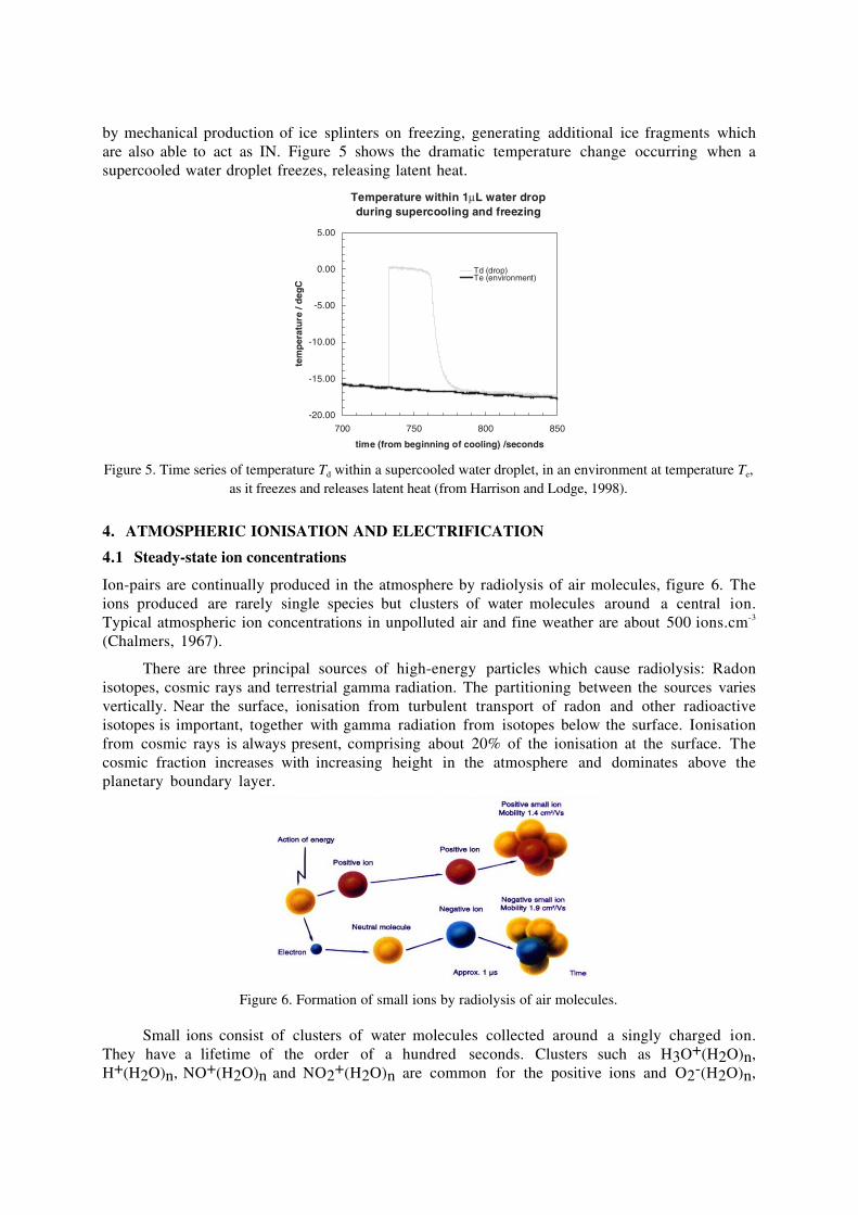
by mechanical production of ice splinters on freezing, generating additional ice fragments whichare also able to act as IN. Figure 5 shows the dramatic temperature change occurring when asupercooled water droplet freezes, releasing latent heat.

Temperature within 1µL water drop during supercooling and freezing

-20.00

-15.00

-10.00

-5.00

0.00

5.00

700 750 800 850

time (from beginning of cooling) /seconds

tem

per

atu

re /

deg

C

Td (drop)Te (environment)

Figure 5. Time series of temperature Td within a supercooled water droplet, in an environment at temperature Te,as it freezes and releases latent heat (from Harrison and Lodge, 1998).

4. ATMOSPHERIC IONISATION AND ELECTRIFICATION

4.1 Steady-state ion concentrations

Ion-pairs are continually produced in the atmosphere by radiolysis of air molecules, figure 6. Theions produced are rarely single species but clusters of water molecules around a central ion.Typical atmospheric ion concentrations in unpolluted air and fine weather are about 500 ions.cm-3

(Chalmers, 1967).

There are three principal sources of high-energy particles which cause radiolysis: Radonisotopes, cosmic rays and terrestrial gamma radiation. The partitioning between the sources variesvertically. Near the surface, ionisation from turbulent transport of radon and other radioactiveisotopes is important, together with gamma radiation from isotopes below the surface. Ionisationfrom cosmic rays is always present, comprising about 20% of the ionisation at the surface. Thecosmic fraction increases with increasing height in the atmosphere and dominates above theplanetary boundary layer.

Figure 6. Formation of small ions by radiolysis of air molecules.

Small ions consist of clusters of water molecules collected around a singly charged ion.They have a lifetime of the order of a hundred seconds. Clusters such as H3O+(H2O)n,H+(H2O)n, NO+(H2O)n and NO2+(H2O)n are common for the positive ions and O2-(H2O)n,

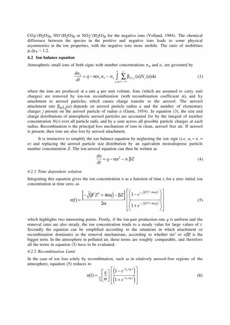
CO4-(H2O)n, NO-(H2O)n or NO2-(H2O)n for the negative ions (Volland, 1984). The chemicaldifference between the species in the positive and negative ions leads to some physicalasymmetries in the ion properties, with the negative ions more mobile. The ratio of mobilitiesm-/m+ ~ 1.2.

4.2 Ion balance equation

Atmospheric small ions of both signs with number concentrations n+ and n- are governed by

dndt

q n n n a N a daj jja

±± ± ±

= -•

•

=

•

= - - ÂÚa bm 10

, ( ) ( ) (3)

where the ions are produced at a rate q per unit volume. Ions (which are assumed to carry unitcharges) are removed by ion-ion recombination (with recombination coefficient a), and byattachment to aerosol particles, which causes charge transfer to the aerosol. The aerosolattachment rate b±1,j(a) depends on aerosol particle radius a and the number of elementarycharges j present on the aerosol particle of radius a (Gunn, 1954). In equation (3), the size andcharge distributions of atmospheric aerosol particles are accounted for by the integral of numberconcentration N(r) over all particle radii, and by a sum across all possible particle charges at eachradius. Recombination is the principal loss mechanism of ions in clean, aerosol free air. If aerosolis present, then ions are also lost by aerosol attachment.

It is instructive to simplify the ion balance equation by neglecting the ion sign (i.e. n+ ª n- =n) and replacing the aerosol particle size distribution by an equivalent monodisperse particlenumber concentration Z. The ion-aerosol equation can then be written as

dndt

q n n Z= - -a b2 (4)

4.2.1 Time dependent solution

Integrating this equation gives the ion concentration n as a function of time t, for a zero initial ionconcentration at time zero, as

n tZ q Z e

e

Z q t

Z q t( ) =

- +( ) -[ ] -ÊË

ˆ¯

+ÊË

ˆ¯

È

Î

ÍÍÍ

˘

˚

˙˙˙

- +( )

- +( )

b a b

a

b a

b a

2 2 4

4

4

2

1

1

2 2

2 2(5)

which highlights two interesting points. Firstly, if the ion-pair production rate q is uniform and theremoval rates are also steady, the ion concentration tends to a steady value for large values of t.Secondly the equation can be simplified according to the situations in which attachment orrecombination dominates as the removal mechanisms, according to whether an2 or nbZ is thebigger term. In the atmosphere in polluted air, these terms are roughly comparable, and thereforeall the terms in equation (5) have to be evaluated.

4.2.2 Recombination Limit

In the case of ion loss solely by recombination, such as in relatively aerosol-free regions of theatmosphere, equation (5) reduces to

n tq e

e

q t

q t( ) =

ÈÎÍ

˘˚˙

-( )+( )

È

Î

ÍÍ

˘

˚

˙˙

-

-a

a

a

1

1

2

2(6)

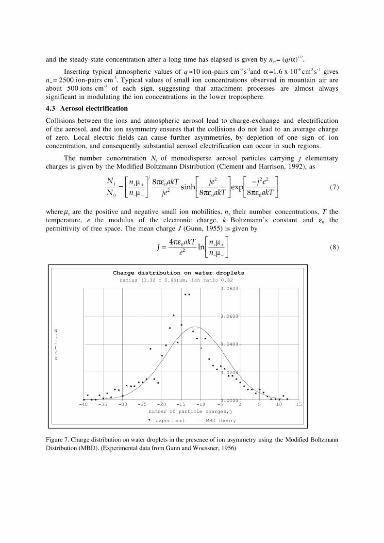
and the steady-state concentration after a long time has elapsed is given by n• = (q/a)1/2.

Inserting typical atmospheric values of q ª10 ion-pairs cm-3 s-1and a =1.6 x 10-6 cm3 s-1 givesn• = 2500 ion-pairs cm-3. Typical values of small ion concentrations observed in mountain air areabout 500 ions cm-3 of each sign, suggesting that attachment processes are almost alwayssignificant in modulating the ion concentrations in the lower troposphere.

4.3 Aerosol electrification

Collisions between the ions and atmospheric aerosol lead to charge-exchange and electrificationof the aerosol, and the ion asymmetry ensures that the collisions do not lead to an average chargeof zero. Local electric fields can cause further asymmetries, by depletion of one sign of ionconcentration, and consequently substantial aerosol electrification can occur in such regions.

The number concentration Nj of monodisperse aerosol particles carrying j elementarycharges is given by the Modified Boltzmann Distribution (Clement and Harrison, 1992), as

N

Nnn

akTje

jeakT

j eakT

jj

0

02

2

0

2 2

0

88 8

=È

ÎÍ

˘

˚˙

È

ÎÍ

˘

˚˙

-È

ÎÍ

˘

˚˙+ +

- -

mm

pepe pe

sinh exp (7)

where m± are the positive and negative small ion mobilities, n± their number concentrations, T thetemperature, e the modulus of the electronic charge, k Boltzmann’s constant and e0 thepermittivity of free space. The mean charge J (Gunn, 1955) is given by

J

akTe

nn

=È

ÎÍ

˘

˚˙+ +

- -

4 02

pe mm

ln (8)

Charge distribution on water dropletsradius (3.32 ± 0.65)µm, ion ratio 0.82

0.0000

0.0200

0.0400

0.0600

0.0800

-40 -35 -30 -25 -20 -15 -10 -5 0 5 10 15

N(j)/Z

number of particle charges,j

experiment MBD theory

Figure 7. Charge distribution on water droplets in the presence of ion asymmetry using the Modified BoltzmannDistribution (MBD). (Experimental data from Gunn and Woessner, 1956)

5. OBSERVED TROPOSPHERIC ELECTRICAL PROPERTIES UNDER NON-THUNDERSTORM CONDITIONS

Many electrical soundings of the atmosphere have been made during disturbed (thunderstorm)conditions, but few such measurements have been made under more quiescent atmosphericconditions. There are difficulties with in-cloud measurements, as a balloon or aircraft platformwill be required: this may itself introduce difficulties with sampling, particularly under smallelectric fields.

Regions of aerosol particles, some of which may acquire appreciable charges, are theprincipal perturbation to atmospheric electric fields under fair weather conditions. In general theupper and lower surfaces of a horizontal region of particles or droplets will charge from ionsflowing vertically as a result of the fair weather conduction current, and the region within the layerwill be of low conductivity compared with that of the surrounding air. Figure 8 shows electricfield profiles observed in non-thunderstorm clouds, which are typically two orders of magnitudesmaller than equivalent profiles determined in thunderstorms.

Figure 8. Typical electric field profiles found in non-thunderstorm clouds under (a) liquid water and (b)supercooled conditions (from MacGorman and Rust, 1998).

electrometer

V to f PLL

SONDE

radio link

RECEIVER f to V Logger

electrodes

PLL

P,T,U

Optical link

Figure 9. Summary schematic of an atmospheric electric field sensor using vertically-spaced spherical electrodes,flown under a conventional radiosonde balloon. The electrometer circuit and batteries are mounted within thelower electrode, with the data conveyed via a voltage-to-frequency converter and an optical link operating at100kHz. A phase-locked loop (PLL), recovers the data from an optical receiver, and the signal is injected into astandard meteorological RS80 radiosonde measuring pressure P, temperature T and relative humidity U. The uhfreceiver recovers the 100kHz signal, which a further PLL converts back to a voltage. The voltage is logged at20Hz by a computer and analogue to digital converter (from Harrison, 2001).

A modern sensor suitable for use in low fields using a standard meteorological radiosondehas recently been described (Harrison, 2001), using the displacement current to detect chargedaerosol particles from the changes caused in electric field. Figure 9 shows a schematic of thesystem, which is disposable. Regions of space charge of ~10nC.m-3 were reported in shallow layers,with electrical structures suggesting electrification by the conduction current.

6. DIRECT INFLUENCES OF ELECTRIFICATION AND RADIOACTIVITY ON CLOUDS

In considering how natural atmospheric ionisation might influence cloud physics or cloudformation, Harrison (2000) identified two possible routes:

(1) direct processes, such as production of new aerosol (e.g. sulphate) by gas-to-particleconversion (GPC) or homogeneous nucleation

(2) indirect processes, such as the modification of existing heterogeneous nucleation processes byaffecting the condensation nuclei (CN) or ice nuclei (IN).

6.1 Direct processes

6.1.1 CN production

In the presence of high levels of radioactivity, the radiolytic formation of particles has been shownto occur. Bricard et al (1968) found the CN concentration could be made to cycle by the regularaddition of Thoron (a short-lived source of a-particles), figure 10. Vohra et al (1984) observedparticle formation in artificial air in the presence of trace concentrations of sulphur dioxide,ozone and ethene, with naturally-occurring radon concentration levels, suggesting that ultrafineaerosol production could occur in atmospheric air under natural conditions. Recent theoreticalwork by Yu and Turco (2001), further strengthens the expectation that radiolytic particleproduction will be found in the atmosphere, and that the conventional ion-aerosol balanceequations are incomplete.

Figure 10. Particles formed in filtered Parisian air, with the addition of regular cycles of Thoron (fromBricard et al, 1968).

6.2 Indirect processes

6.2.1 Scavenging of charged particles

The removal of aerosol particles by cloud droplets, scavenging, is known to be influenced bymany factors, including electrical forces (Pruppacher and Klett, 1997). Figure 11 shows thepartitioning of the water drop charge Qd in response to the image charge induced by the charged

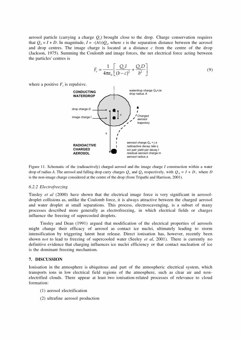
aerosol particle (carrying a charge Qa) brought close to the drop. Charge conservation requiresthat Qd = I + D. In magnitude, I = -(A/s)Qa, where s is the separation distance between the aerosoland drop centres. The image charge is located at a distance c from the centre of the drop(Jackson, 1975). Summing the Coulomb and image forces, the net electrical force acting betweenthe particles' centres is

F

Q Ib c

Q Dbe

a a=-

+ÈÎÍ

˘˚

14 0

2 2pe ( )(9)

where a positive Fe is repulsive.waterdrop charge Qd=Jedrop radius ACONDUCTING

WATERDROP

RADIOACTIVECHARGEDAEROSOL

image charge I

drop charge D

aerosol charge Qa = j eradioactive decay rate hion pair yield per decay Iresidual aerosol charge maerosol radius a

Chargedaerosoltrajectory

s

c

Figure 11. Schematic of the (radioactively) charged aerosol and the image charge I construction within a waterdrop of radius A. The aerosol and falling drop carry charges Qa and Qd respectively, with Q d = I + D , where Dis the non-image charge considered at the centre of the drop (from Tripathi and Harrison, 2001).

6.2.2 Electrofreezing

Tinsley et al (2000) have shown that the electrical image force is very significant in aerosol-droplet collisions as, unlike the Coulomb force, it is always attractive between the charged aerosoland water droplet at small separations. This process, electroscavenging, is a subset of manyprocesses described more generally as electrofreezing, in which electrical fields or chargesinfluence the freezing of supercooled droplets.

Tinsley and Dean (1991) argued that modification of the electrical properties of aerosolsmight change their efficacy of aerosol as contact ice nuclei, ultimately leading to stormintensification by triggering latent heat release. Direct ionisation has, however, recently beenshown not to lead to freezing of supercooled water (Seeley et al, 2001). There is currently nodefinitive evidence that charging influences ice nuclei efficiency or that contact nucleation of iceis the dominant freezing mechanism.

7. DISCUSSION

Ionisation in the atmosphere is ubiquitous and part of the atmospheric electrical system, whichtransports ions in low electrical field regions of the atmosphere, such as clear air and non-electrified clouds. There appear at least two ionisation-related processes of relevance to cloudformation:

(1) aerosol electrification

(2) ultrafine aerosol production

7.1 Aerosol electrification

Stratified regions of aerosol will charge in the atmosphere under quiescent conditions as a resultof ion transport by the conduction current. Although the charges carried are unlikely to besufficiently large to initiate bulk discharge processes such as lightning, the distribution of chargesexpected on aerosols under natural ion asymmetry may yield a small fraction of particles withsignificant charge levels. Such highly-charged aerosol would normally be rapidly neutralised byatmospheric ionisation, but in ion-depleted regions arising from large aerosol concentrations,moderately-high charge levels might persist.

Scavenging processes are influenced by aerosol charge; the water drop charge hasnegligible effect by comparison. Since heterogeneous ice nucleation requires the collection ofsuitable aerosol able to operate as ice nuclei, it is therefore conceivable that aerosol chargingcould influence ice formation. If charge were itself shown to be a enhancing effect for ice nuclei,then the synergy between the effects of increased collection and efficient nuclei could be potent.

7.2 Ultrafine particle production

Radiolytic particle production has been observed in laboratory air at atmospheric levels ofionisation, but the particles formed are small and not, at their formation, able to act as cloudcondensation nuclei. The recent theoretical work of Yu and Turco (2001) is, however, compelling,in that it shows that in aerosol-deficient regions, such as marine stratus cloud, cosmic rayionisation could provide an appreciable source of particles. Further microphysical modelling isrequired to show that sufficient ultrafine particles can survive to become cloud condensationnuclei before the effect on suitable clouds can be assessed.

8. CONCLUSIONS

The physical processes, if any, leading to the cosmic ray-low cloud correlation observed by Marshand Svensmark (2000) remain to be established in the atmosphere. As discussed above, there areatmospheric electrical mechanisms relating ionisation to cloud which remain relatively unexploredin atmospheric physics, and in suitable cloud, could conceivably offer physical explanations forthe observed correlation. However without numerical and theoretical estimates of theirsignificance, it is currently impossible to regard ionisation effects as irrelevant to cloud processes.

REFERENCES

Bricard F., Billard F. and Madelaine G., (1968), Formation and evolution of nuclei ofcondensation that appear in air initially free of aerosols, J. Geophys. Res., 54, 39-52

Chalmers J.A. (1967), Atmospheric Electricity, 2nd edition, Pergamon Press, Oxford

Clement C.F. and Harrison R.G. (1992), The charging of radioactive aerosols J. Aerosol Sci. 23, 5,481-504

Gunn R. (1954), Diffusion charging of atmospheric droplets by ions, and the resultingcombination coefficients, J. Meteorol., 11, 339

Gunn R. (1955), The statistical electrification of aerosols by ionic diffusion, J. Coll. Sci., 10, 107-119

Gunn R. and Woessner R.H. (1956), Measurements of the systematic electrification of aerosols, J.Coll. Sci., 11, 254-259

Harrison R.G. (1997), Climate change and the global atmospheric electrical system Atmos.Environ. 31, 20, 3483-3484

Harrison R.G. (2000), Cloud formation and the possible significance of charge for atmosphericcondensation and ice nuclei Space Science Reviews, 94, 381-396

Harrison R.G. (2001), A balloon-carried electrometer for high-resolution atmospheric electricfield measurements in clouds Rev Sci Inst, 72, 6, 2738-2741

Harrison R.G. and Lodge B.N. (1998), A calorimeter to detect freezing in supercooled waterdroplets Rev Sci Inst, 69, 11, 4004-4005

Jackson J.D. (1975), Classical Electrodynamics Wiley

Marsh N.D. and Svensmark H. (2000), Low cloud properties influenced by cosmic rays, Phys.Rev. Lett., 85, 23, 5004-5007

MacGorman D.R. and Rust W.D. (1998), The electrical nature of storms, OUP

Pruppacher, H.R. and Klett, J.D., (1997). Microphysics of clouds and precipitation, 2nd edition,Kluwer

Rogers and Yau (1989), A short course in Cloud Physics, Pergamon Press

Seeley L.H., Seidler G.T. and Dash J.G., (2001), Laboratory investigation of possible icenucleation by ionizing radiation in pure water at tropospheric temperatures, J. Geophys. Res., 106,D3, 3033-3036,2001

Tinsley B.A. and Dean G.W (1991) Apparent tropospheric response to MeV-GeV particle fluxvariations: a connection via electrofreeezing of supercooled water in high-level clouds? J GeophysRes 96, pp22283-22296

Tinsley, B.A., Rohrbaugh R.P., Hei M., and Beard K.V., (2000), Effects of image charges on thescavenging of aerosol particles by cloud droplets, and on droplet charging and possible icenucleation processes, J. Atmos Sci., 57, 2118-2134.

Tripathi S.N. and Harrison R.G. (2001), Scavenging of electrified radioactive aerosol, AtmosEnviron, (in press)

Vohra K.G., Subba Ramu M.C.and Muraleedharan T.S. (1984), An experimental study of the rôleof radon and its daughters in the conversion of sulphur dioxide into particles in the atmosphere,Atmos. Env., 18, 8, 1653-1656

Volland H. (1984), Atmospheric electrodynamics, Springer-Verlag, Berlin

Wilson C.T.R. (1929), Some thundercloud problems, J. Franklin Institute, 208, 1-12

Yu F. and Turco R.P. (2001) From molecular clusters to nanoparticles: the rôle of ambientionisation in tropospheric aerosol formation J. Geophys. Res. 106, D5, 4797-4814

TROPOSPHERIC ION MEASUREMENTS

K L. Aplin* and R. G. HarrisonDepartment of Meteorology, The University of Reading, PO Box 243, Earley Gate, Reading,RG6 6BB UK

AbstractTo investigate ion-induced nucleation in the atmosphere experimentally,it is necessary to select only the circumstances when ion-induced effectsare likely to dominate, and identify and exclude times when othermeteorological factors are influencing ion concentrations. To do this,reliable ion, aerosol and meteorological measurements at the same site arerequired, with analysis of different weather conditions. A methodologyfor identifying the effects of meteorological conditions on the localatmospheric electrical environment is discussed, based on ion andmeteorological measurements made at Reading in the spring and summerof 2000. It is found that even under virtually identical synopticmeteorological conditions, there is significant variability in the ionconcentration.

1. INTRODUCTION

Atmospheric small ions are produced near the Earth's surface by natural radioactivity and cosmicrays; the electrical conductivity of the air s is proportional to the total ion concentration n. Inequilibrium, the concentration of small ions is modulated by the ion production rate and theatmospheric aerosol concentration (e.g. MacGorman and Rust, 1998). Meteorological factors alsohave an important effect on s, for example, suspended aerosol particles are wind-borne, and maybe advected to locally reduce the ion concentration by attachment. The links betweenmeteorology and atmospheric electricity are tacitly acknowledged, but surprisingly little effort hasbeen made to quantify the relationship between them. Chalmers' (1967) discussion was typical ofmuch of the atmospheric electricity literature, clearly recognising meteorological effects onconductivity, but giving little explanation of the causal links.

Atmospheric water drops carry an electric charge, and therefore conditions such as fog andhaze can cause perturbations to atmospheric electrical measurements, both directly (electrically)and by condensation onto the insulators essential in measuring apparatus. Periods of stableatmospheric electrical conditions, however, are necessary for consistent measurements. In theclassical paradigm of “fair-weather” atmospheric electricity, Ohm’s law relates the airconductivity s, vertical charge flux density J and vertical potential gradient E, as

J = sE (1)

(e.g. MacGorman and Rust, 1998). Conditions under which fair-weather properties can beexpected were only summarised relatively recently by Reiter (1992), who excluded periods whenhydrometeors were present at the surface. High cloud and fair-weather cumulus were permittedwith this classification, until the cumulus started to become grey at the base indicating that it wasbeginning to charge. However, Barlow and Harrison (1999) showed experimentally that non-electrified clouds perturb the surface atmospheric electric field by thermal influences on theturbulent transport of charged particles and ions. * Now at Rutherford Appleton Laboratory, Space Science and Technology Department, Chilton Didcot, BerksOX11 OQX, UK.

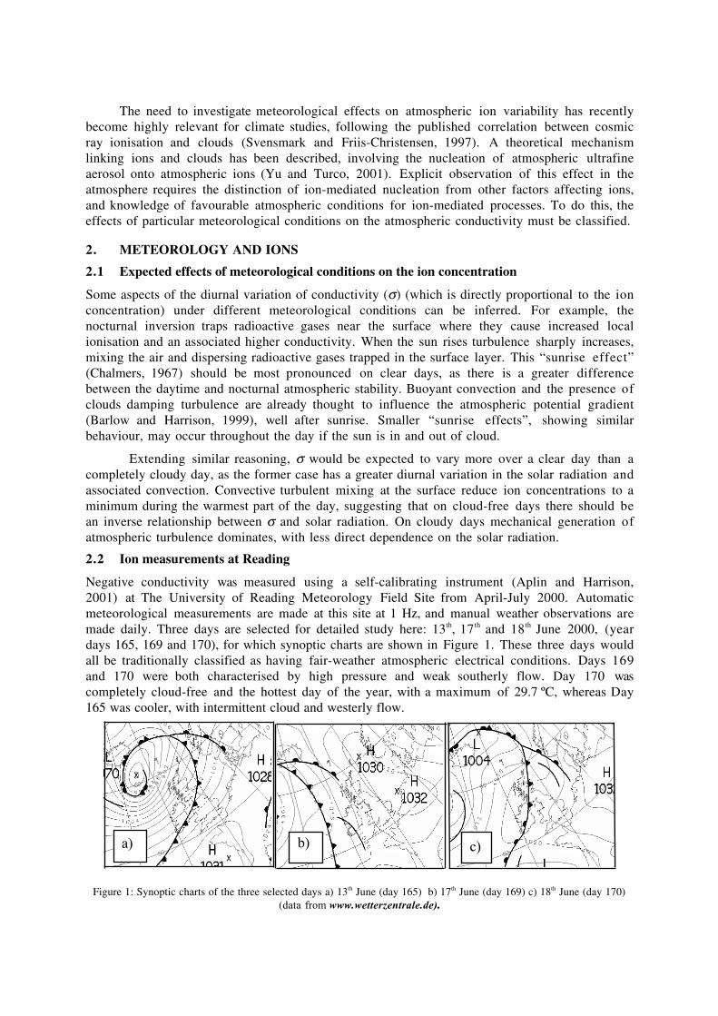
The need to investigate meteorological effects on atmospheric ion variability has recentlybecome highly relevant for climate studies, following the published correlation between cosmicray ionisation and clouds (Svensmark and Friis-Christensen, 1997). A theoretical mechanismlinking ions and clouds has been described, involving the nucleation of atmospheric ultrafineaerosol onto atmospheric ions (Yu and Turco, 2001). Explicit observation of this effect in theatmosphere requires the distinction of ion-mediated nucleation from other factors affecting ions,and knowledge of favourable atmospheric conditions for ion-mediated processes. To do this, theeffects of particular meteorological conditions on the atmospheric conductivity must be classified.

2. METEOROLOGY AND IONS

2.1 Expected effects of meteorological conditions on the ion concentration

Some aspects of the diurnal variation of conductivity (s) (which is directly proportional to the ionconcentration) under different meteorological conditions can be inferred. For example, thenocturnal inversion traps radioactive gases near the surface where they cause increased localionisation and an associated higher conductivity. When the sun rises turbulence sharply increases,mixing the air and dispersing radioactive gases trapped in the surface layer. This “sunrise effect”(Chalmers, 1967) should be most pronounced on clear days, as there is a greater differencebetween the daytime and nocturnal atmospheric stability. Buoyant convection and the presence ofclouds damping turbulence are already thought to influence the atmospheric potential gradient(Barlow and Harrison, 1999), well after sunrise. Smaller “sunrise effects”, showing similarbehaviour, may occur throughout the day if the sun is in and out of cloud.

Extending similar reasoning, s would be expected to vary more over a clear day than acompletely cloudy day, as the former case has a greater diurnal variation in the solar radiation andassociated convection. Convective turbulent mixing at the surface reduce ion concentrations to aminimum during the warmest part of the day, suggesting that on cloud-free days there should bean inverse relationship between s and solar radiation. On cloudy days mechanical generation ofatmospheric turbulence dominates, with less direct dependence on the solar radiation.

2.2 Ion measurements at Reading

Negative conductivity was measured using a self-calibrating instrument (Aplin and Harrison,2001) at The University of Reading Meteorology Field Site from April-July 2000. Automaticmeteorological measurements are made at this site at 1 Hz, and manual weather observations aremade daily. Three days are selected for detailed study here: 13th, 17th and 18th June 2000, (yeardays 165, 169 and 170), for which synoptic charts are shown in Figure 1. These three days wouldall be traditionally classified as having fair-weather atmospheric electrical conditions. Days 169and 170 were both characterised by high pressure and weak southerly flow. Day 170 wascompletely cloud-free and the hottest day of the year, with a maximum of 29.7 ºC, whereas Day165 was cooler, with intermittent cloud and westerly flow.

a) b) c)

Figure 1: Synoptic charts of the three selected days a) 13th June (day 165) b) 17th June (day 169) c) 18th June (day 170)(data from www.wetterzentrale.de).

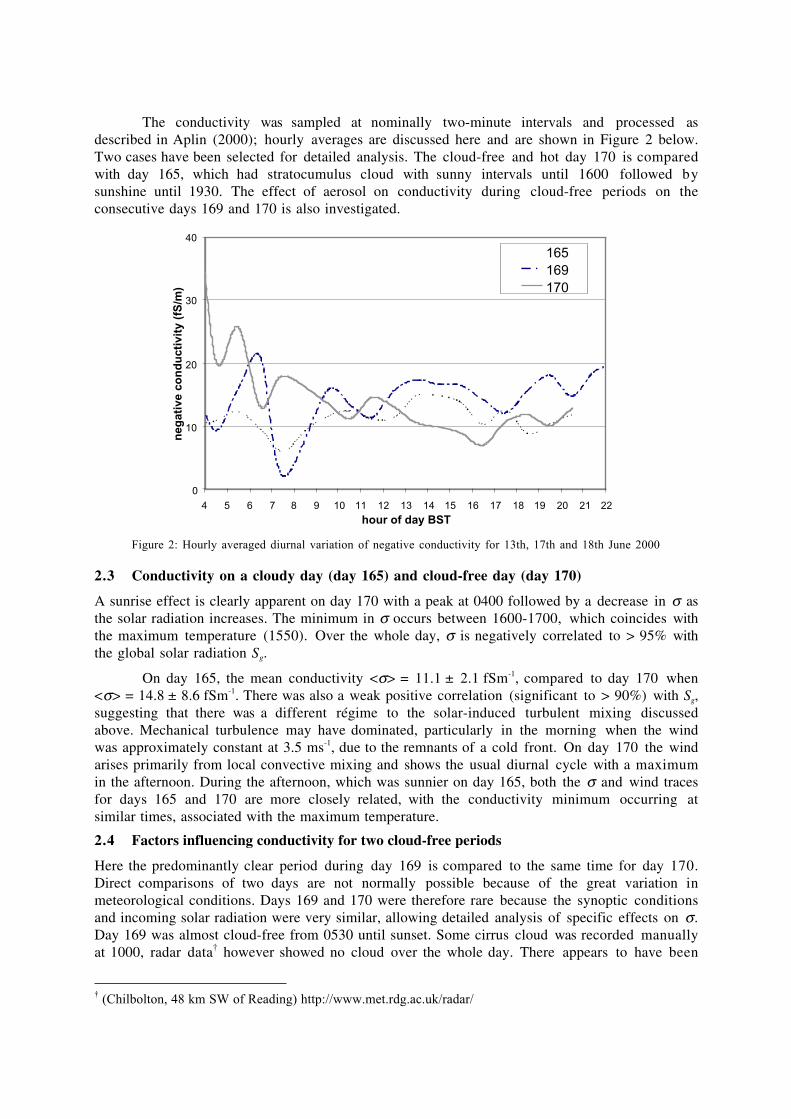
The conductivity was sampled at nominally two-minute intervals and processed asdescribed in Aplin (2000); hourly averages are discussed here and are shown in Figure 2 below.Two cases have been selected for detailed analysis. The cloud-free and hot day 170 is comparedwith day 165, which had stratocumulus cloud with sunny intervals until 1600 followed bysunshine until 1930. The effect of aerosol on conductivity during cloud-free periods on theconsecutive days 169 and 170 is also investigated.

0

10

20

30

40

4 5 6 7 8 9 10 11 12 13 14 15 16 17 18 19 20 21 22hour of day BST

neg

ativ

e co

nd

uct

ivit

y (f

S/m

)

165169170

Figure 2: Hourly averaged diurnal variation of negative conductivity for 13th, 17th and 18th June 2000

2.3 Conductivity on a cloudy day (day 165) and cloud-free day (day 170)

A sunrise effect is clearly apparent on day 170 with a peak at 0400 followed by a decrease in s asthe solar radiation increases. The minimum in s occurs between 1600-1700, which coincides withthe maximum temperature (1550). Over the whole day, s is negatively correlated to > 95% withthe global solar radiation Sg.

On day 165, the mean conductivity <s> = 11.1 ± 2.1 fSm-1, compared to day 170 when<s> = 14.8 ± 8.6 fSm-1. There was also a weak positive correlation (significant to > 90%) with Sg,suggesting that there was a different régime to the solar-induced turbulent mixing discussedabove. Mechanical turbulence may have dominated, particularly in the morning when the windwas approximately constant at 3.5 ms-1, due to the remnants of a cold front. On day 170 the windarises primarily from local convective mixing and shows the usual diurnal cycle with a maximumin the afternoon. During the afternoon, which was sunnier on day 165, both the s and wind tracesfor days 165 and 170 are more closely related, with the conductivity minimum occurring atsimilar times, associated with the maximum temperature.

2.4 Factors influencing conductivity for two cloud-free periods

Here the predominantly clear period during day 169 is compared to the same time for day 170.Direct comparisons of two days are not normally possible because of the great variation inmeteorological conditions. Days 169 and 170 were therefore rare because the synoptic conditionsand incoming solar radiation were very similar, allowing detailed analysis of specific effects on s.Day 169 was almost cloud-free from 0530 until sunset. Some cirrus cloud was recorded manuallyat 1000, radar data† however showed no cloud over the whole day. There appears to have been

† (Chilbolton, 48 km SW of Reading) http://www.met.rdg.ac.uk/radar/

some cloud present at Reading from the radiometer measurements, but it is likely to have beenthin or high cloud with little impact on the surface conditions.

Despite the very similar weather on days 169 and 170 (see Table 1), the conductivitieswere different and did not show the same variation, with a correlation coefficient r = –0.26between them. This suggests that other processes cause the variability, such as changes in theaerosol concentration. s could also be sensitive to small changes in meteorological variables suchas the wind speed. PM10 mass concentrations M are measured at a site 2 km NW of the Universityfield site‡, and are therefore used to infer bulk properties of the air mass. M was almost twice ashigh on day 169 as day 170, probably because of the increased traffic on a Saturday. Thecorrelation coefficient between M and s was negative on day 169 and positive to > 98% on day170. Ion-aerosol theory (e.g. Clement and Harrison, 1992) predicts a negative correlation betweenaerosol and s. Although the theory links aerosol number concentration and s, these observationsshow the expected general relationship between mass concentration and s. The lower s maytherefore have been caused by higher local wind speeds associated with high aerosolconcentrations.

Table 1: Average conductivity, meteorological conditions, aerosol mass concentration and correlation (r) between Mand s for 0530-1830 on 17th and 18th June 2000

Day <s> – st. dev. (fSm-1) <u> (ms-1) RH(%) Dirn (deg) <M> (mgm-3) r (M,s)

169 12.9˚– 4.7˚ 3.7 65 142 23.6 -0.20170 14.7˚– 4.4˚ 3.0 62 112 13.7 +0.64

In strong insolation, photochemical aerosol production would further complicate thevariability in the conductivity. Dhanorkar and Kamra (1997) showed that small charged aerosolparticles contribute directly to s, rather than inversely by the conventional theory. The positive M-s correlation on day 170 might therefore be caused by charged photochemically-producedaerosol particles.

2.5 Effect of aerosol on conductivity for day 169

It is possible to estimate the expected effect of aerosol on the ion concentration by using classicalion-aerosol theory. The rate of change of the ion concentration n in the presence of an aerosolnumber concentration Z is given by the ion balance equation

dndt

q n nZ np= - - -a b g2 (2)

where q is the ionisation rate, a an ion-ion recombination coefficient, b an ion-aerosol attachmentcoefficient, g an ion-induced nucleation coefficient, which is probably exponentially proportionalto the ion concentration, where 0 > p ≥ 2, depending on the nucleation mechanism. Inequilibrium, there should be an inverse relationship between n and Z because of ion-aerosolattachment. As this was observed on day 169, the effect of aerosol on s on day 169 was calculatedto investigate the different conductivity variations compared to day 170 (when classical ion-aerosol theory did not apply over the whole day). The ion balance equation (2) was used toestimate the ion concentration n, and hence the conductivity s, from the aerosol concentration,assuming equilibrium and that

s mª ne (3)

with an assumed mean mobility for negative ions of 1.9 x 10-4 m2V-1s-1 (e.g. Dolezalek, 1974).

‡ http://www.aeat.co.uk/netcen/airqual/

The mass concentration M (mass per unit volume) and the number concentration Z of amonodisperse aerosol population are related by

M Z r=

ÊËÁ

ˆ¯

43

3p r (4)

where r is the particle density. This equation was used to estimate Z from M assuming the averageradius of the population (2 mm) and that the particles are ammonium sulphate, with r = 1.77 gcm-3

(Khlystov et al, 2001). The coefficients a and q were assumed to be 1.6 x 10-6 cm3s-1 and 10 cm-

3s-1 respectively. b was calculated from Gunn’s (1954) expression, and is a function of the meanradius, temperature and mean charge j (assumed to be –1e). The aerosol was split into three sizemodes, nucleation with mean radius rn = 0.25 mm, accumulation with ra = 0.88 mm and coarse withrc = 5.6 mm (Seinfeld and Pandis, 1998).

The average sensitivity of the conductivity to a 1% change in the aerosol numberconcentration in each mode was calculated from equation 5. For the initially assumed sizedistribution, (shown in Table 2) with 80% of the particles in the fine mode and only 5% in thecoarsest size range, the conductivity is most sensitive to changes in the coarse mode. This is notwhat would intuitively be expected, because there are fewest particles in the coarse mode, and fromthe ion balance equation (2), the number of particles controls the conductivity, by attachment.Another factor affecting the availability of particles to attach is their surface area. This was testedby fixing the surface area-Z product, by increasing the number of particles in the nucleation andaccumulation modes. The nucleation mode was most sensitive to changes in Z; therefore fortypical aerosol size distributions, the surface area of the coarse aerosol dominates over thenumber.

Table 2 Characteristics of the assumed aerosol distribution, and calculated sensitivities to a 1% change in aerosolnumber concentration.

Mode Nucleation Accumulation CoarseAssumed fraction of particles 0.8 0.15 0.05Mean radius (mm) 0.25 0.88 5.6

Sensitivity to 1% change in Z 0.13% 0.11% 0.22%Sensitivity to 1% change in Z(surface area x Z fixed)

0.2% 0.0% 0.0%

One finding is that conductivity is relatively insensitive to changes in the aerosolpopulation, which may be significant because of the discussion whether conductivity can be usedas an indicator of urban aerosol pollution (see e.g. Aplin, 2000). In this case, changes in theaerosol concentration are not significant enough to account for the observed conductivityvariation on day 169, therefore other sources of variability in the conductivity dominate.

3. CONCLUSIONS

The conductivity of air in the surface layer is relatively insensitive to the aerosol concentration atthe atmospheric concentrations observed; therefore most of its variability is likely to be due tometeorological factors. The different conductivities measured on two days which were a) almostidentical synoptically and b) conformed to “fair weather” in the strictest classical sense, implythat the ion concentration is sensitive to small changes in meteorological variables. The traditional“fair-weather” classification, which aims to ensure consistent and comparable measurements,therefore appears inadequate. Furthermore, it does not allow for electro-meteorologicalinteractions and excludes other sources of atmospheric electrical variability.

The majority of atmospheric electricity and aerosol measurements made at the surface inEngland probably occur in non fair-weather conditions, for which there is little understanding ofthe variability in anything other than general terms. There is evidence that cloud affects surfaceatmospheric electrical conditions by modulating atmospheric stability. We propose an extension tothe existing classification: (1) fair-weather: as Reiter’s (1992) definition, but cloud-free, withvariability caused almost entirely by micrometeorological factors (2) semi-fair-weather: presentingsimilar atmospheric electrical conditions to (1), but identified primarily by meteorological stabilitycriteria with no local charge generation, rather than solely the absence of electrified clouds and (3)non-fair-weather. Extension of the classical fair-weather paradigm to include data obtained oncloudy days, and more detailed investigation of micrometeorological effects on conductivity isimportant if the ion-induced effects hypothesised to contribute to aerosol production are to beunambiguously identified.

ACKNOWLEDGEMENTS

The experimental work was supported by the UK Natural Environment Research Council. KLA’sattendance at the IACI meeting was funded by the Environmental Sciences Department, Universityof Hertfordshire.

REFERENCES

Aplin K.L. (2000), Instrumentation for atmospheric ion measurements, PhD. Thesis, TheUniversity of Reading, UK

Aplin K.L. and Harrison R.G. (2001), Rev. Sci. Instrum., 72, 8, in press

Barlow J.F and Harrison R.G. (1999), In Christian H.J. (ed) Proceedings 11th InternationalConference on Atmospheric Electricity, Guntersville, Alabama 7th-11th June 1999NASA/CP-1999-209261, 575-578

Chalmers J.A. (1967), Atmospheric Electricity, 2nd edition, Pergamon Press, Oxford

Clement C.F. and Harrison R.G. (1992), J. Aerosol Sci. 23, 5, 481-504

Dhanorkar S. and Kamra A.K. (1997), J. Geophys. Res. 102, D25, 30147-30159

Dolezalek H. (ed.) (1974), Electrical processes in atmospheres, Springer Verlag, Darmstadt

Gunn R. (1954), J. Meteorol., 11, 339

Khlystov A., Kos G. P. A., ten Brink H.M., Mirme A., Tuch T., Roth C. and Kreyling W.G. (2001),Atm. Env., 35, 11, 2045-2051

MacGorman D.R. and Rust W.D. (1998), The electrical nature of storms, OUP

Reiter R. (1992), Phenomena in atmospheric and environmental electricity, Elsevier, Amsterdam

Seinfeld J.H. and Pandis S.N. (1998), Atmospheric chemistry and physics, Wiley, New York

Svensmark H. and Friis-Christensen E. (1997), J. Atmos. Solar-Terrestrial Phys, 59, 1225-1232

Yu F. and Turco R.P. (2001). J. Geophys. Res. 106, D5, 4797-4814.

ATMOSPHERIC AEROSOLS: FORMATION AND GROWTH

Markku KulmalaUniversity of Helsinki, Department of Physical Sciences, Division of Atmospheric Sciences,P.O. Pox 64, FIN-00014, University of Helsinki, Finland

1. INTRODUCTION

It is widely recognised that the increasing atmospheric concentrations of greenhouse gases such ascarbon dioxide and methane can potentially drive a significant warming process of the earth’sclimate. However, a topic of more recent attention is the possibility that increased atmosphericconcentrations of aerosol particles might drive a significant radiative forcing process of the planet(see, for example, Charlson et al., 1992; and Charlson and Wigley, 1994). The increased aerosolconcentrations are largely due to secondary particle production i.e. homogeneous nucleation fromvapour precursors. The secondary aerosols have both natural and anthropogenic origin. Aerosolparticles influence the climate by two distinct mechanisms: the direct reflection of solar radiationby aerosol particles, and the indirect increase in cloud reflectivity caused by enhanced number ofcloud condensation nuclei. IPCC (1996) has reported that uncertainties in the estimation of directand indirect aerosol effects on global climate are big (see Fig. 1.). These uncertainties arise largelyfrom the limited information on the spatial and temporal distribution of aerosols and clouds.However, recently some progress has been made in evaluating the radiative effects of variousaerosol components such as sulfate, organics, black carbon, sea-salt, and crustal species (Chuang etal., 1997; Haywood and Ramaswamy, 1998; Kaufman and Fraser, 1997; Winter and Chylek, 1997;Sokolik and Toon, 1996).

Despite these efforts, substantial uncertainties still remain in quantifying the contributionfrom each source, particularly, for biogenic and natural emissions, including organic vapours.Without understanding the contribution of natural emissions of aerosols and particles to radiativeforcing, we can never hope to accurately predict or understand the true effect of anthropogenicemissions.

Among the key questions in reducing error bars are how aerosol particles are formed, howthey will grow from clusters of a few molecules to CCN sizes (>100 nm) and how they will formcloud droplets. Once formed, clouds have a very extensive influence on the Earth's radiationbudget through their albedo and greenhouse effects. With global warming, future cloud propertiesare likely to change due to the warmer and moister conditions, and possibly due to increasedaerosol particle emissions from both primary (e.g. wind generated sea-spray) and secondaryaerosols (from biogenically and anthropogenically influenced gas-to-particle conversionprocesses). Clouds are however rather crudely presented in global and regional climate models(GCM, RCM). Processes, such as nucleation, droplet activation during condensation, diffusivegrowth, droplet evaporation, droplet coalescense and conversion to raindrops, are very crudelytaken into account in present-day atmospheric large-scale models. For example, we have recentlyshown the importance of aerosol formation and growth processes to CCN concentrations (Kulmalaet al., 2000) as well as the effect of nitric acid and other semivolatile gases in influencing cloudformation processes, in particular, in enhancing the cloud droplet population, thereby increasingcloud reflectance (Kulmala et al., 1993; Laaksonen et al., 1997). The importance of includingmulti-component aerosol populations, and the dynamic feedback in the cloud forming processes,along with the importance of coupling chemical and physical processes in predicting clouddroplet populations have been illustrated by O’Dowd et al., (1999a; 1999b).

Particle formation and growth in the atmosphere have recently received growingexperimental and theoretical interest. Therefore, instrumental techniques for measuringconcentrations of freshly formed particle have been developed, and particles with diameter of

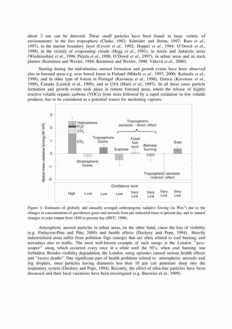
about 3 nm can be detected. These small particles have been found in large variety ofenvironments: in the free troposphere (Clarke, 1992; Schröder and Ström, 1997; Raes et al.,1997), in the marine boundary layer (Covert et al., 1992; Hoppel et al., 1994; O’Dowd et al.,1998), in the vicinity of evaporating clouds (Hegg et al., 1991), in Arctic and Antarctic areas(Wiedensohler et al., 1996; Pirjola et al., 1998; O’Dowd et al., 1997), in urban areas and in stackplumes (Kerminen and Wexler, 1994; Kerminen and Wexler, 1996; Väkevä et al., 2000).

Starting during the mid-nineties, aerosol formation and growth events have been observedalso in forested areas e.g. over boreal forest in Finland (Mäkelä et al., 1997, 2000; Kulmala et al.,1998), and in other type of forests in Portugal (Kavouras et al., 1998), Greece (Kavouras et al.,1999), Canada (Leaitch et al., 1999), and in USA (Marti et al., 1997). In all these cases particleformation and growth events took place in remote forested areas, where the release of highlyreactive volatile organic carbons (VOCs) from trees followed by a rapid oxidation to low volatileproducts, has to be considered as a potential source for nucleating vapours.

3

1

2

0

-1

-2

C O2

C H4

N O2Halocarbons

StratosphericOzone

TroposphericOzone

Sulphate

Fossilfuelsoot Biomass

burning

Tropospheric aerosols-indirect effect

Solar

Troposphericaerosols - direct effect

Confidence level

High Low Low Low Very Low

Very Low

Very Low

Very Low

Glo

bal m

ean

radi

ativ

e fo

rcin

g (W

/m2 )

Figure 1: Estimates of globally and annually averaged anthropogenic radiative forcing (in Wm-2) due to thechanges in concentrations of greenhouse gases and aerosols from pre-industrial times to present day and to naturalchanges in solar output from 1850 to present day (IPCC, 1996).

Atmospheric aerosol particles in urban areas, on the other hand, cause the loss of visibility(e.g. Finlayson-Pitts and Pitts, 2000) and health effects (Dockery and Pope, 1994). Heavilyindustrialized areas suffer from pollution fogs (smogs) that are often related to coal burning andnowadays also to traffic. The most well-known example of such smogs is the London ”pea-souper” smog, which occurred every once in a while until the 50’s, when coal burning wasforbidden. Besides visibility degradation, the London smog episodes caused serious health effectsand ”excess deaths”. One significant part of health problems related to atmospheric aerosols andfog droplets, since particles having diameters less than 10 mm can penetrate deep into therespiratory system (Dockery and Pope, 1994). Recently, the effect of ultra-fine particles have beendiscussed and their local variations have been investigated (e.g. Buzorius et al., 1999).

2. AEROSOL DYNAMICS

During the processes of formation and growth of atmospheric aerosols the aerosol dynamics,atmospheric chemistry and meteorology form a coupled system. The importance of atmosphericchemistry (e.g. Pirjola and Kulmala, 1998; Pirjola 1999) as well as meteorological conditions(Nilsson and Kulmala, 1998; Nilsson et al., 2000; Väkevä et al., 2000) on particle formation andgrowth have been demonstrated under tropospheric conditions. Although ternary nucleation ofwater-ammonia-sulphuric acid vapours (Korhonen et al., 1999) has shown to be able to explainatmospheric nucleation – i.e. formation of ~1 nm particles - in many cases (Kulmala et al., 2000),the exact routes for formation of 3 nm particles are still unclear, because besides nucleation, alsothe growth from 1 nm size to 3 nm size is needed.

In order to be able to understand the formation and growth processes of atmosphericaerosols and cloud droplets their thermodynamic properties should be known. For example, in thecondensation process, the driving force is the vapour pressure difference between gas phase andsurface. However, in the atmosphere where there are multicomponent, multiphase mixtures, theirthermodynamic state and phase diagrams are typically very complex. It is very important to obtainthermodynamically consistent vapour pressures, chemical activities, surface tensions and densitiesfor organic and inorganic compounds and their water solutions (for the importance see e.g.Korhonen et al., 1999) as a function of temperature and composition.

In future, development of nucleation theories, modelling and nucleation rateparameterizations are needed. So far, conclusions on whether or not certain substances causenucleation in the atmosphere conditions are usually based on predictions given by the classicalnucleation theory (CNT). CNT treats the nucleating molecular clusters as macroscopic dropletswhich is a questionable approach since the nucleating clusters often contain less than fiftymolecules. Nucleation of various vapors using molecular dynamics (MD) and Monte Carlo (MC)simulation techniques is needed to investigate. So far, some investigations were carried out usingab initio calculations on small sulfuric acid-water clusters (Arstila et al 1998), classical MD(Laasonen et al, 2000) and MC (Vehkamäki and Ford, 1999) simulations of argon nucleation, aswell as DFT calculations of nucleation in binary systems imitating water and different organicmolecules (Laaksonen et al., 1995, Napari and Laaksonen 2000). Also, a new nucleationmechanism based on stable dimers (Lushnikov and Kulmala, 1998) has been proposed.

In contrast to laboratory conditions, the formation of aerosol in the atmosphere can bekinetically limited by some of the intermediate steps of its formation processes. The equilibriumstate is thus not necessarily the aerosol itself but can be, for example, thermodynamically stableclusters (TSC), as we have recently shown (Kulmala et al., 2000). Although there is strongindication that the water-sulphuric acid-ammonia nucleation mechanism (Korhonen et al., 1999)explains the formation of new atmospheric aerosols (diameter < 3 nm) in many circumstances, thecondensation of these vapors does not explain the observed growth rates of the particles (Kulmalaet al., 2000), and in atmospheric conditions nucleation and growth are decoupled (Kulmala et al.,2000). The other possible relevant nucleation mechanism is ion-induced nucleation.

Aerosol dynamic modelling (nucleation, condensation, coagulation, deposition) with gasphase chemistry to obtain the atmospheric significance of nucleation and condensation ofdifferent vapours have been and will be performed. The aerosol dynamics and atmosphericchemistry model used in the present research is based on the model recently developed by ourresearch group (Pirjola and Kulmala, 1998; Pirjola 1999). In these models aerosol formation andgrowth including aerosol dynamics to evaluate sink terms for condensable molecules and gasphase chemistry to include source terms for these molecules will be used. Process models will becoupled with dispersion models. In the chemistry part of the model the chemistry of O3, NOx, VOCand other relevant species will be related to aerosol formation. The effects of meteorologicaldynamics on aerosol processes will be studied by applying the aerosol dynamic models in a

Lagrangian approach including wave motions and atmospheric mixing. The results shows thatternary water-ammonia-sulphuric acid system is proper candidate for atmospheric aerosolformation.

3. FORMATION AND GROWTH OF ATMOSPHERIC AEROSOLS, FIELDEXPERIMENTS

Formation and growth of aerosol particles have been observed and will be observed at atmosphericconditions. Our research group has participated in several field campaigns. These includescontinuous measurements performed at our field stations and several international intensivecampaigns like Aerosol Characterisation Experiment 1 and 2 in 1994 and 1997 (ACE-1 and ACE-2 organised by IGAC), International Arctic Ocean Expeditions 1991 and 1996, Biogenic aerosolformation in the boreal forest (BIOFOR, 1997-1999, SMEAR stations, Finland, Hyytiälä), Newparticle formation and fate in the coastal environment (PARFORCE, Mace Head, Ireland), andongoing the OSOA (Origin and Formation of Secondary Organic Aerosol) experiment. As anexample we consider here BIOFOR results in more detailed.

All data measured during the BIOFOR campaigns are available on the Biofor web pageshttp://mist.helsinki.fi/Biofor/index.html (ask for usercode and password from the correspondingauthor). In addition to the numerical data there are also a number of plots produced as a result ofthe analysis of the data. The data are classified into 9 subgroups: 1) aerosol total numberconcentration and size distribution measurements in the size range 3-800 nm, 2) aerosolchemistry, 3) aerosol and gas fluxes by eddy covariance and gradient methods, 4) measurementsof meteorological parameters and gas concentrations at six different levels from the mast, 5)meteorology of boundary layer and trajectories, 6) concentrations and emissions of BVOC(biological volatile organic compounds), 7) ground level concentrations of inorganic gases, 8)measurements of the size distribution of wet (ambient) aerosol from 0.5-32 _m at 18 m height,and 9) solar radiation measurements. The detailed descriptions of the instruments used are givenon the web pages.

When the particle formation event occurs, the mode of the fresh particles appears into themeasurement range. In Figure 2. aerosol number size distributions measured using DifferentialMobility Particle Sizer (DMPS) during a typical nucleation event day are shown. The nucleationmode practically dominates the spectrum with its high number concentration during thenucleation burst. For this event, particle growth from nucleation mode up to accumulation mode isclearly observable. The growth is frequently seen to continue during the following days up toaccumulation mode (see also Kulmala et al., 2001).

00 03 06 09 12 15 18 21 0010

3

104

105

Time of day (hr)

Figure 2: Aerosol size distributions measured by DMPS from 2m height inside the forest (6.4. 1999).

00 03 06 09 12 15 18 21 00103

104

105

TSI3010 67mTSI3025 67m

Time of day (hr)

Figure 3: Aerosol concentrations measured by CPC’s above the forest heights 67m and 18m (6.4. 1999).

During the events, aerosol fluxes determined using an eddy covariance technique areobserved to be downwards. Also the measurements made by Condensation Particle Counters (CPC)and DMPS at different heights support this finding. From particle flux data, using the eddycovariance method (Buzorius et al., 1998), usually a small overall downward flux is observed. Thedownward flux clearly increases during nucleation events, with an exception of the cases when thesurface wind was from direction of 220-250∞ (direction of the Tampere city and the Hyytiäläinstitute buildings). Then a strong upward particle flux is observed due to local surface-levelpollution.

The difficulties in absolute calibration of the DMPS set ups as well as sampling losses in thelines suggested that the gradient of particles will be best determined placing two identical CPCpairs in the mast (18 m and 67 m height). The CPC pairs consisted of the ultrafine CPC (TSI Inc3025) for determination of the particles larger than 3 nm in diameter and conventional CPC (TSIInc. 3010) for particles larger than 10 nm in diameter. The difference of the reading of the CPC’sgives an approximate value for the ultrafine mode particle concentrations in the beginning of theburst. The data from the CPC pairs is shown for the event day of 6 April 1999 in Figure 3. Thedifference between the CPC readings from the two levels shows that the ultrafine particles havehigher concentrations in higher level during the nucleation burst. This result will support theparticle flux data that illustrate a net loss of particles to the canopy; however, it does notnecessarily indicate a particle source at the top of the boundary layer or higher altitudes, eventhough nucleation is more probable in these regions.

4. CONCLUSIONS

According to recent results on atmospheric aerosol formation some preliminary conclusions canbe made on atmosphere aerosol formation. (see Kulmala et al., 2001)

The most probable formation mechanism is ternary nucleation (water – sulphuric acid –ammonia) and the growth to observable sizes takes place mainly owing to condensation of organicvapours. Nevertheless, there is no direct proof of this phenomenon because the composition of1–5 nm size particles is very difficult to determine using present state-of-art instrumentation. Theother possible nucleation mechanism is ion induced nucleation with sulphuric acid and watervapours.

Nucleation takes place typically in very specific weather conditions: e.g. in Hyytiälä in coldair advection in Polar and Arctic air masses, at low cloudiness, and no precipitation. Furthermore,the nucleation was closely connected to the onset of strong turbulence in the morning-noontransition from stable to unstable stratification, which should also correspond to the onset ofconvection and entrainment from aloft.

The emission rates for several gaseous compounds have been determined (Kulmala et al.,2001). Using four independent ways the amount of the condensable vapour needed for observedgrowth of aerosol particles was estimated to 2-10 x 107 vapour molecules cm-3. The estimations forsource rate gives 7.5-11 x 104 cm-3s-1.

REFERENCES

Arstila H., Laasonen K. and Laaksonen A, (1998) J. Chem. Phys., 108, 1031.

Buzorius, G., U. Rannik, J.M. Mäkelä, T. Vesala and M. Kulmala (1998) J. Aerosol. Sci. 29, 157.

Buzorius, G., Hämeri, K., Pekkanen, J. and Kulmala M. (1999) Atmospheric Environment 33, 553.

Buzorius, G., Ü. Rannik, J. M. Mäkelä, P. Keronen, T. Vesala, M. Kulmala. (2000) J. Geophys.Res. 105, 19905.

Charlson, R.J., and Wigley, T.M.L. 1994. Sulphate aerosol and climatic change. ScientificAmerican, 270, 48-57.

Charlson, R.J., Schwartz, S.E., Hales, J.M., Cess, R.D., Coakley, J.A., Hansen, J.E. and Hofmann,D.J. 1992. Climate forcing by anthropogenic aerosols. Science, 255, 423-430.

Clarke, A.D. 1992. Atmospheric nuclei in the remote free troposphere. J. Atmos. Chem., 14, 479-488.

Covert, D.S., Kapustin, V.N., Quinn, P.K., and Bates, T.S. 1992. New particle formation in themarine boundary layer. J. Geophys. Res., 97, 20581 – 20587.

Chuang C. C., Penner J. E., Taylor K. E., Grossman A. S. and Walton J. J. (1997). J. Geophys. Res.102, 3761.

Dickerson, R.R., Kondragunta, S., Stenchikov, G., Civerolo, K.L., Doddridge, B.G. and Holben,B.N. (1997) Science 278, 827.

Dockery, D.W. and Pope, C.A. (1994) Annu. Rev. Public. Health, 15, 107.

Finlayson-Pitts B.J. and Pitts, Jr. J.N. (2000) Chemistry of the upper and lower atmosphere.Academic Press, San Diego.

Hämeri, K., Väkevä, M., Hansson, H.-C. and Laaksonen A. (2000) J. Geophys. Res. 105, 22231.

Haywood J. M. and Ramaswamy V. (1998) J. Geophys. Res. 103, 6043.

Hegg, D.A., Radke, L.F. and Hobbs, P.V. 1991. Measurements of Aitken nuclei and cloudcondensation nuclei in the marine atmosphere and their relation to the DMS-cloud-climatehypothesis. J. Geophys. Res., 96, 18727-18733.

Hoppel, W.A., Frick, G.M., Fitzgerand, J.W. and Larson, R.E. 1994. Marine boundary layermeasurements of new particle formation and the effects nonprecipitating clouds have onaerosol size distribution. J. Geophys. Res., 99, 14443-14459.

IPCC (Intergovernmental Panel on Climate Change) 1996. Climate Change 1995 (Edited byHoughton J.T., Meira Filho L.G., Gallander B.A:, Harris N., Kattenberg A. and MaskellK.). Cambridge University Press, Cambridge

Kaufman Y. J. and Fraser R. S. (1997) Science 277, 1636.

Kavouras, I.G., Mihalopoulos, N. and Stephanou, E.G. 1998. Formation of atmospheric particlesfrom organic acids produced by forests. Nature, 395, 683-686

Korhonen, P., Kulmala, M., Laaksonen, A., Viisanen, Y., McGraw, R. and Seinfeld, J.H. 1999.Ternary nucleation of H2SO4, NH3 and H2O in the atmosphere. J. Geophys. Res., 104,26,349-26,353.

Kulmala, M., A. Laaksonen, P. Korhonen, T. Vesala, T. Ahonen, J.C. Barrett, (1993) J. Geophys.Res. 98, 22949.

Kulmala, M., Laaksonen A., Charlson R.J. and Korhonen P. (1997) Nature, 388, 336.

Kulmala, M., A. Toivonen, J. M. Mäkelä and A. Laaksonen, 1998. Analysis of the growth ofnucleation mode particles observed in Boreal forest. Tellus, 50B, 449-462.

Kulmala, M., Pirjola, L. and Mäkelä, J.M. 2000. Stable sulphate clusters as a source of newatmospheric particles. Nature, 404, 66-69.

Kulmala, M., K. Hämeri, P.P. Aalto, J.M. Mäkelä, L. Pirjola, E.D. Nilsson, G. Buzorius, U. Rannik,M. dal Maso, W. Seidl, T. Hoffman, R. Janson, H.-C. Hansson, Y. Viisanen, A. Laaksonen,and C.D. O’Dowd. 2001. Overviwe of the internal project on biogenic aerosol formationin the boreal forest (BIOFOR). Tellus 53B, 324-343.

Laaksonen, A. Talanquer, V., and Oxtoby, D.W (1995) Annu. Rev. Phys. Chem., 46, 489.

Laaksonen, J. Hienola, M. Kulmala, F. Arnold, (1997) Geophys. Res. Lett. 24, 3009.

Laaksonen, P. Korhonen, M. Kulmala, R.J. Charlson, (1998) J. Atmos. Sci. 55, 853.

Laasonen, K., , S. Wonzack, R. Strey and A. Laaksonen, J. Chem. Phys. (in press)

Leaitch, W.R., Bottenheim, J.W., Biesenthal, T.A., Li, S.M., Liu, P.S.K., Asalian, K., Dryfhoutclark,H., Hopper, F. and Brechtel, F. 1999. A case study of gas-to-particle conversion in aneastern Canadian forest. J. Geophys. Res. 104, 8095-8111.

Lushnikov, A.A., Kulmala, M. (1998) Phys. Rev. Lett. 81, 5165.

Marti, J.J., Weber, R.J., McMyrry, P.H., Eisele, F., Tanner, D., and Jefferson A. 1997. New particleformation at a remote continental site: Assessing the contributions of SO2 and organicprecursors. J. Geophys. Res. 102, 6331-6339.

Mäkelä, J.M., Aalto, P., Jokinen, V., Pohja, T., Nissinen, A., Palmroth, S., Markkanen, T., Seitsonen,K., Lihavainen, H., and Kulmala, M. 1997. Observations of ultrafine aerosol particleformation and growth in boreal forest, Geophys. Res. Lett., 24, 1219-1222.

Mäkelä, J.M., Koponen, I.K., Aalto, P. and Kulmala, M. 2000. One-year data of submicron sizemodes of tropospheric background aerosol in Southern Finland. J. Aerosol Sci., 31, 595-611.

Napari, A. Laaksonen, L. (2000) Phys. Rev. Lett. 84, 2184.

Nilsson, E.D. and Kulmala, M. 1998. The potential for atmospheric mixing processes to enhancethe binary nucleation rate. J. Geophys. Res., 103, 1381-1389.

Nilsson, E.D., Pirjola, L. and Kulmala, M. 2000. The effect of atmospheric waves on aerosolnucleation and size distribution. J. Geophys. Res., 105, 19,917-19,926.

O’Dowd, C.D., Lowe, J.A., Smith, M.H., Davison, B., Hewitt, C.N. and Harrison, R.M. 1997.Biogenic sulphur emissions and inferred non-sea-salt-sulphate cloud condensation nucleiin and around Antarctica, J. Geophys. Res., 102, 12,839-12,854.

O’Dowd, C.D., Geever, M., Hill, M.K., Jennings, S.K., and Smith, M.K. 1998. New particleformation and spatial scales in the clean marine coastal environment. Geophys. Res. Lett.,25, 1661-1664

O’Dowd, C. D., J. A. Lowe, M. H. Smith and A. D. Kaye (1999a) Q. J. R.. Meteorol. Soc., 125,1295.

O'Dowd, CD, J.A. Lowe, and MH Smith (1999b) Geophys. Res. Letts, 26, 1311.

Seckmeyer, G., Mayer, B., Bernhard, G., Erb, R., Albold, A., Jäger, H. and Stockwell, W.R. (1997)Atmospheric Environment 34, 2971.

Pirjola, L. 1999. Effects of the increased UV radiation and biogenic VOC emissions on ultrafinesulphate aerosol formation. J. Aerosol Sci., 30, 355-367

Pirjola, L. and Kulmala, M. 1998. Modelling the formation of H2SO4-H2O particles in rural, urbanand marine conditions. Atmos. Res., 46, 321-347.

Pirjola, L., Laaksonen, A., Aalto, P., and Kulmala, M. 1998. Sulfate aerosol formation in the Arcticboundary layer. J. Geophys. Res., 103, 8309-8322.

Raes, F., Van Dingenen, R., Cuevas, E., Van Velthoven, P.F.J., and Prospero, J.M. 1997.Observations of aerosols in the free troposphere and marine boundary layer of thesubtropical Northeast Atlantic: Discussion of processes determining their size distribution,J. Geophys. Res., 102, 21315-21328.

Schröder, F. and Ström, J. 1997. Aircraft measurements of submicrometer aerosol particles (> 7nm) in the midlatitude free troposphere and tropopause region. Atmos. Res., 44, 333-356.

Seinfeld, J.H. and Pandis (1998) Atmospheric Chemistry and Physics. (Wiley)

Sokolik I. N. and Toon O. B. (1996) Nature 381, 681.

Vehkamäki, H., and I. J. Ford, (1999) J. Chem. Phys., 112, 4193.

Viisanen, Y. (1991) Ph.D.Thesis, University of Helsinki, Department of Physics.

Viisanen, Y., Strey, R., Reiss, H., (1993) J. Chem. Phys., 99, 4680.

Viisanen, Y., Strey, R., Reiss, H. (2000) J. Chem. Phys., 112, 8205

Viisanen, Y., Strey, R. (1996) J. Chem. Phys., 105, 8293

Viisanen, Y., Kulmala, M., Laaksonen, A., (1997) J. Chem. Phys., 107, 920

Väkevä, M., Hämeri, K., Puhakka, T., Nilsson, E.D., Hohti, H. and Mäkelä, J.M. 2000. Effects ofmeteorological processes on aerosol particle size distribution in an urban backgroundarea, J. Geophys. Res., 105, 9807-9821.

Winter B. and Chylek P. (1997)Tellus 49B, 72.

COSMIC RAYS, PARTICLE FORMATION, NATURAL VARIABILITYOF GLOBAL CLOUDINESS, AND CLIMATE IMPLICATIONS

Fangqun YuAtmospheric Sciences Research Center, State University of New York, Albany, New York, USA

AbstractVia its role in aerosol formation, cosmic ray may affect the globalcloudiness and hence climate. Here we show that an increase in cosmicray fluxes may lead to an increase in particle production in the lowertroposphere but a decrease in particle production in the uppertroposphere. In addition to the reported positive correlation betweencosmic ray variations and low cloudiness, our analysis of satellite-basedcloud cover data reveals that high cloudiness may be anti-correlated withcosmic ray variations if volcano and El Niño impacts are excluded. Theobserved different correlations between cosmic ray variations and low,middle and high cloud anomalies are consistent with the predicteddifferent sensitivities of particle production to cosmic ray changes atvarious altitudes. The influence of the solar-modulated cosmic ray fluxeson global cloudiness, if confirmed, may provide the external forcingneeded to reconcile the apparent differences between observed surfaceand troposphere temperature trends.

1. INTRODUCTION

Clouds play a key role in the energy budget of Earth’s surface and lower atmosphere, and areprobably the largest contributor to the uncertainty concerning the global climate change1. Smallmodifications of the amount, distribution, or radiative properties of clouds can have significantimpacts on the predicted climate2. To detect and attribute anthropogenic influences on climate, itis crucial to quantify the natural fluctuations of cloudiness and the associated radiative forcing. In1997, Svensmark and Friis-Christensen3 reported a surprising discovery that total cloud cover overmidlatitude ocean correlates closely with the galactic cosmic ray (GCR) intensity. The cloud dataanalyzed include the C2 data sets from the International Satellite Cloud Climatology Project(ISCCP)4. Recently it has become possible to infer global cloud properties at different altitudesfrom the ISCCP-D2 data, which come from an improvement of procedures leading to the C2data5. Analyses of the ISCCP-D2 data indicate that a clear correlation can only be seen betweenGCR fluxes and the global average of low cloud cover6,7. Due to its potential importance andimplication, the GCR-cloud-climate hypothesis3 has been under close scrutiny8-10. Two of the mainquestions and doubts raised against the hypothesis are: (1) no convincing physical mechanism isavailable to explain the correlation, (2) there is no obvious correlation between solar activity andhigh cloudiness (where, it is argued, if GCR ionization has any impact on cloud microphysics, itwould most likely be found in the upper troposphere where GCR incidence is greatest).

Here we first try to address these two raised issues by investigating the role of GCRionization in particle formation and the potential altitude-dependent influence of GCR variationson particle production and global cloudiness. We then explore the possibility of GCR-inducedglobal cloud changes as an external forcing that may reconcile the apparent differences in globalmean temperature trends between ground and atmosphere measurements. Over the last twodecades, the temperature records taken at the Earth's surface show rapid warming (globally 0.15 ±0.05 oC per decade), however the data produced by satellite and balloon studies indicate little ifany warming (globally 0.05 ± 0.10 oC per decade) of the low to mid-troposphere - the

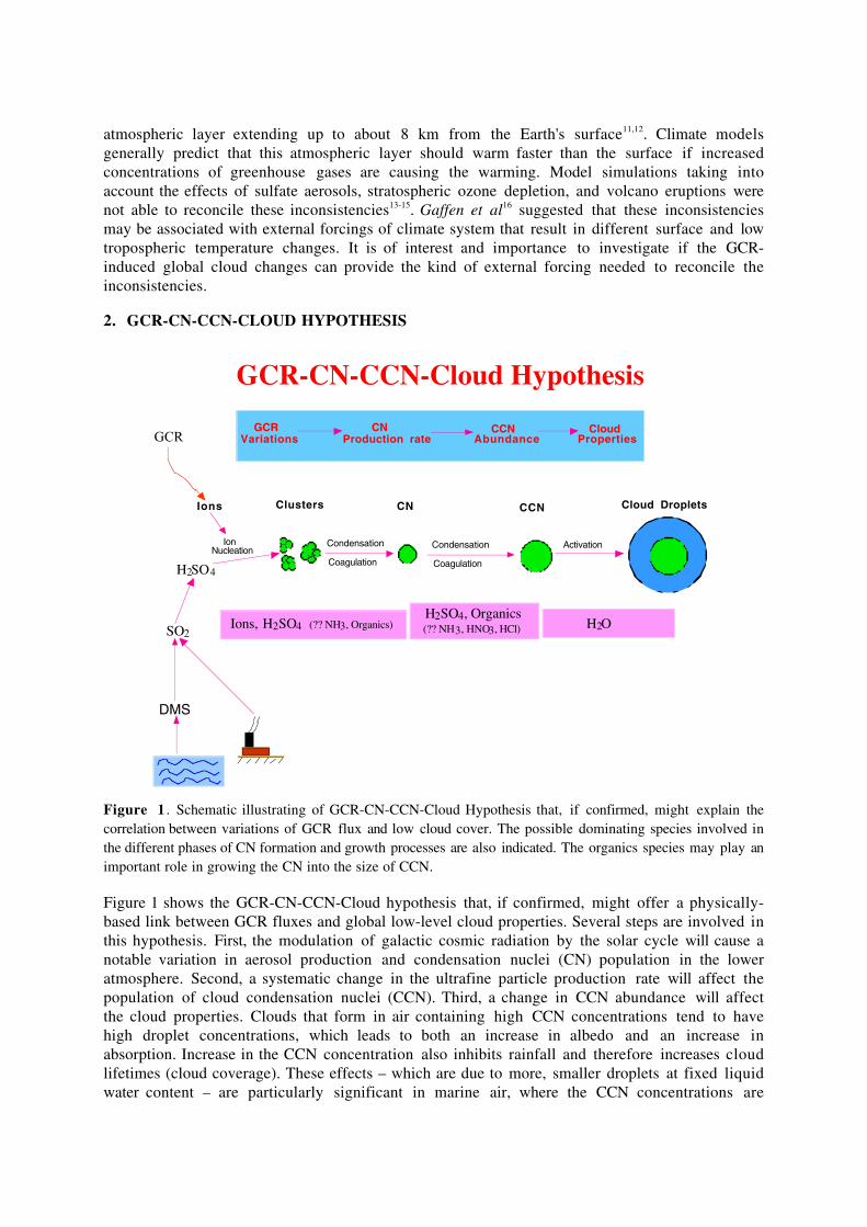
atmospheric layer extending up to about 8 km from the Earth's surface11,12. Climate modelsgenerally predict that this atmospheric layer should warm faster than the surface if increasedconcentrations of greenhouse gases are causing the warming. Model simulations taking intoaccount the effects of sulfate aerosols, stratospheric ozone depletion, and volcano eruptions werenot able to reconcile these inconsistencies13-15. Gaffen et al16 suggested that these inconsistenciesmay be associated with external forcings of climate system that result in different surface and lowtropospheric temperature changes. It is of interest and importance to investigate if the GCR-induced global cloud changes can provide the kind of external forcing needed to reconcile theinconsistencies.

2. GCR-CN-CCN-CLOUD HYPOTHESIS

Figure 1 . Schematic illustrating of GCR-CN-CCN-Cloud Hypothesis that, if confirmed, might explain thecorrelation between variations of GCR flux and low cloud cover. The possible dominating species involved inthe different phases of CN formation and growth processes are also indicated. The organics species may play animportant role in growing the CN into the size of CCN.

Figure 1 shows the GCR-CN-CCN-Cloud hypothesis that, if confirmed, might offer a physically-based link between GCR fluxes and global low-level cloud properties. Several steps are involved inthis hypothesis. First, the modulation of galactic cosmic radiation by the solar cycle will cause anotable variation in aerosol production and condensation nuclei (CN) population in the loweratmosphere. Second, a systematic change in the ultrafine particle production rate will affect thepopulation of cloud condensation nuclei (CCN). Third, a change in CCN abundance will affectthe cloud properties. Clouds that form in air containing high CCN concentrations tend to havehigh droplet concentrations, which leads to both an increase in albedo and an increase inabsorption. Increase in the CCN concentration also inhibits rainfall and therefore increases cloudlifetimes (cloud coverage). These effects – which are due to more, smaller droplets at fixed liquidwater content – are particularly significant in marine air, where the CCN concentrations are

H2SO4

SO2

DMS

GCR

Ion Nucleation

Condensation

Coagulation

CN CCN

Ions, H2SO4 (?? NH3, Organics) H2SO4, Organics (?? NH3, HNO3, HCl)

Condensation

Coagulation

Activation

GCR-CN-CCN-Cloud Hypothesis

Clusters Cloud Droplets

CN Production rate

CCNAbundance

Cloud Properties

GCR Variations

H2O

Ions

generally quite low. In our proposed hypothesis, the first key process connecting GCR flux andlow cloud cover is that ions generated by GCR ionization play an important role in new particleformation in the lower atmosphere which is the focus of discussion of the next section.

3. COSMIC RAY IONIZATION AND PARTICLE FORMATION

Ambient ions are continuously generated by galactic cosmic rays at the rate of ~2 ion-pairs cm-3s-1

at ground level and up to ~20-30 ion-pairs cm-3s-1 in the upper troposphere17,18. Due to enhancedgrowth and stability of charged clusters (as a consequence of electrostatic interactions), air ionsproduced from GCR ionization may play an important role in the production of new particlesunder typical tropospheric conditions19,20. The proposed ion-mediated nucleation (IMN) theorycan physically explain the enhanced growth rate (a factor of ~ 10) of sub-nanometer clusters andthe square of sulfuric vapor concentration ([H2SO4]

2) dependence of nucleation rate as observedby Weber et al21, and seems to account consistently for ultrafine aerosol formation in jet plumes,in clean continental air and in marine boundary layer, as well as for the diurnal variation in theatmospheric mobility spectrum, as demonstrated by Yu and his colleagues 19,20,22-24.

It is generally known that sulfuric acid vapor concentration ([H2SO4]), temperature (T),relative humidity (RH), pressure (P), and the surface area of preexisting particles are among thelist of parameters controlling the particle formation in the troposphere. The IMN theory addsanother important parameter-ion concentration ([ion], or ionization rate Q)-to this list. Here wefocus on investigating the influence of GCR variations on particle formation and CN abundance atdifferent altitudes. We employ an advanced particle microphysics (APM) model that simulates asize-resolved multicomponent aerosol system via a unified collisional mechanism involving bothneutral and charged particles down to molecular sizes20. The size-resolved ion-ion recombinationcoefficients, ion-neutral collision kernels, and neutral-neutral interaction coefficients calculated inthe model are physically consistent and naturally altitude (temperature, pressure, and relativehumidity) dependent20. For the simulations presented below, the ion concentration is initialized as

Q /a where a is ion-ion recombination coefficient. The pre-existing particles are initialized astwo log-normal modes with total number densities of 19.5/cm3 and 0.6/cm3, median dry diametersof 0.09 mm and 0.3 mm, and standard deviations of 1.6 and 1.5, respectively. This gives an initialwet surface area of ~ 4.5 mm2/cm3 at 90% relative humidity, corresponding to a cloud-processedclean air mass where typical significant aerosol nucleation has been observed.

Figure 2 shows the total condensation nuclei bigger than 3nm (Nd>3 nm) after three hours ofsimulations as a function of ionization rates at three different altitudes (0, 5, 8 km). The values of[H2SO4], T, P, and RH for each altitude (as specified in the figure legend) are fixed during thethree-hour simulations. The shaded areas in Figure 1 are the ranges of Q values corresponding tolow (>680 mb), middle (440-680 mb), and high (<440 mb) cloud regions as defined in ISCCPcloud data according to the cloud top pressures. It is clear from Figure 2 that significant numberof ultrafine particles have formed under all the considered conditions. Most of these newlyformed particles began as electrically charged clusters that have the advantage of enhancedgrowth and stability due to electrostatic effects. The neutral sub-critical clusters, on the other hand,grow too slowly to exceed the critical size under the prevailing conditions. The production rate ofultrafine particles is most sensitive to [H2SO4] and [ion] (or ionization rate). [H2SO4] controls thegrowth rate of ion clusters, while [ion] determines the lifetime of charged clusters and theavailability of ions. The neutralization by ion-ion recombination will make the growing chargedclusters lose their growth advantage and the resulting neutral clusters may dissociate if smallerthan the critical size. At typical [H2SO4] where nucleation has been observed, for very low Q mostof the ion clusters have sufficient time to reach the larger stable sizes prior to recombination andthe nucleation rate is limited by Q. As Q increases, ion concentration increases but the lifetime ofions decreases and hence the fraction of ions having sufficient time to grow to the larger stablesizes decreases. As a result, the total number of particles nucleated first increases but later on

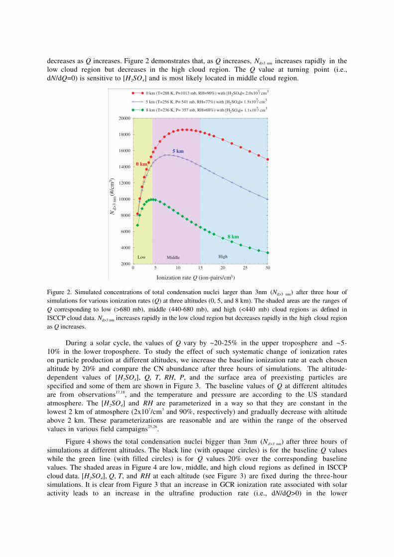
decreases as Q increases. Figure 2 demonstrates that, as Q increases, Nd>3 nm increases rapidly in thelow cloud region but decreases in the high cloud region. The Q value at turning point (i.e.,dN/dQ=0) is sensitive to [H2SO4] and is most likely located in middle cloud region.

Figure 2. Simulated concentrations of total condensation nuclei larger than 3nm (Nd>3 nm) after three hour ofsimulations for various ionization rates (Q) at three altitudes (0, 5, and 8 km). The shaded areas are the ranges ofQ corresponding to low (>680 mb), middle (440-680 mb), and high (<440 mb) cloud regions as defined inISCCP cloud data. Nd>3 nm increases rapidly in the low cloud region but decreases rapidly in the high cloud regionas Q increases.

During a solar cycle, the values of Q vary by ~20-25% in the upper troposphere and ~5-10% in the lower troposphere. To study the effect of such systematic change of ionization rateson particle production at different altitudes, we increase the baseline ionization rate at each chosenaltitude by 20% and compare the CN abundance after three hours of simulations. The altitude-dependent values of [H2SO4], Q, T, RH, P, and the surface area of preexisting particles arespecified and some of them are shown in Figure 3. The baseline values of Q at different altitudesare from observations17,18, and the temperature and pressure are according to the US standardatmosphere. The [H2SO4] and RH are parameterized in a way so that they are constant in thelowest 2 km of atmosphere (2x107/cm3 and 90%, respectively) and gradually decrease with altitudeabove 2 km. These parameterizations are reasonable and are within the range of the observedvalues in various field campaigns25,26.

Figure 4 shows the total condensation nuclei bigger than 3nm (Nd>3 nm) after three hours ofsimulations at different altitudes. The black line (with opaque circles) is for the baseline Q valueswhile the green line (with filled circles) is for Q values 20% over the corresponding baselinevalues. The shaded areas in Figure 4 are low, middle, and high cloud regions as defined in ISCCPcloud data. [H2SO4], Q, T, and RH at each altitude (see Figure 3) are fixed during the three-hoursimulations. It is clear from Figure 3 that an increase in GCR ionization rate associated with solaractivity leads to an increase in the ultrafine production rate (i.e., dN/dQ>0) in the lower

0 5 10 15 20 25 30

Ionization rate Q (ion-pairs/cm3)

2000

4000

6000

8000

10000

12000

14000

16000

18000

20000N

d>3

nm (

#/cm

3 )

0 km (T=288 K, P=1013 mb, RH=90%) with [H2 SO 4 ]= 2.0x10 7 / cm3

5 km (T=256 K, P= 541 mb, RH=77%) with [H

8 km (T=236 K, P= 357 mb, RH=68%) with [H

2 SO 4 ]= 1.5x10 7 / cm3

2 SO 4 ]= 1.1x10 7 / cm3

Low Middle High

0 km

5 km

8 km

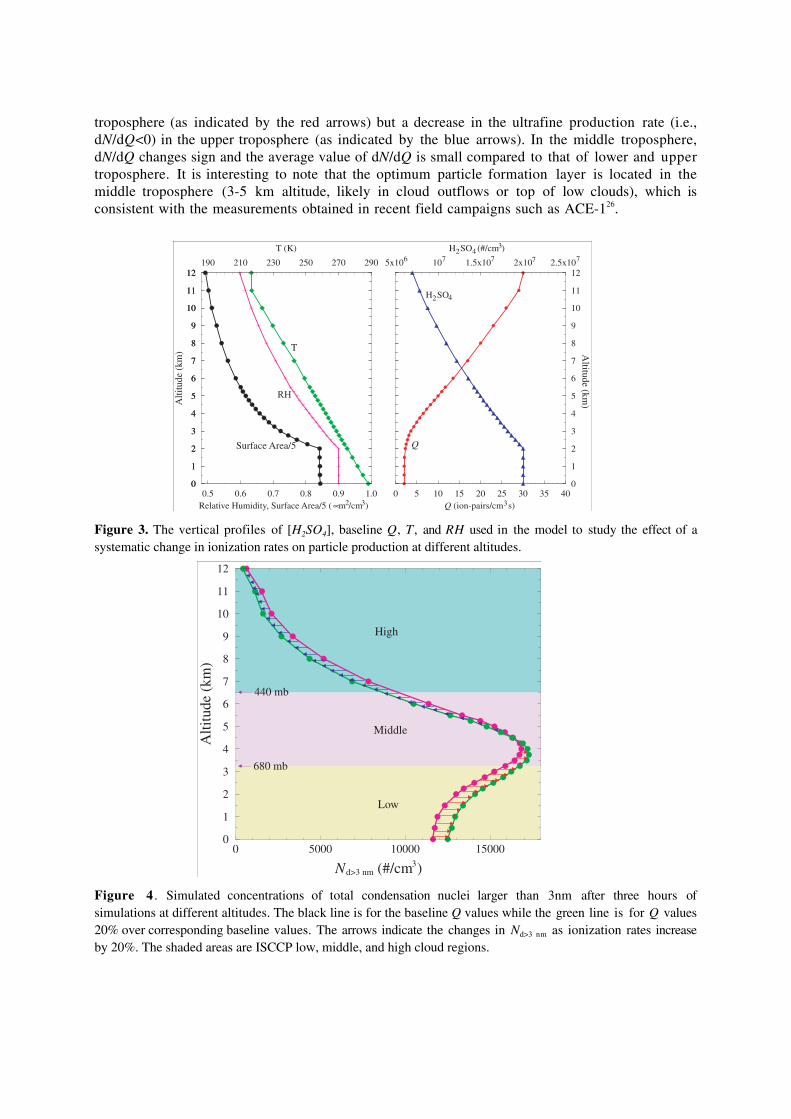
troposphere (as indicated by the red arrows) but a decrease in the ultrafine production rate (i.e.,dN/dQ<0) in the upper troposphere (as indicated by the blue arrows). In the middle troposphere,dN/dQ changes sign and the average value of dN/dQ is small compared to that of lower and uppertroposphere. It is interesting to note that the optimum particle formation layer is located in themiddle troposphere (3-5 km altitude, likely in cloud outflows or top of low clouds), which isconsistent with the measurements obtained in recent field campaigns such as ACE-126.

0 5 10 15 20 25 30 35 40Q (ion-pairs/cm3s)

190 210 230 250 270 290

T (K)

0

1

2

3

4

5

6

7

8

9

10

11

12

T

5x10 10 1.5x10 2x10 2.5x10

H2SO4 (#/cm3)

0

1

2

3

4

5

6

7

8

9

10

11

12

Altitude (km

)

H2SO4

0.5 0.6 0.7 0.8 0.9 1.0Relative Humidity, Surface Area/5 ( µm2/cm3)

0

1

2

3

4

5

6

7

8

9

10

11

12

Alti

tude

(km

)

Surface Area/5

6 7 7 7 7

Q

RH

Figure 3. The vertical profiles of [H2SO4], baseline Q, T , and RH used in the model to study the effect of asystematic change in ionization rates on particle production at different altitudes.

0 5000 10000 15000

Nd>3 nm (#/cm3)

0

1

2

3

4

5

6

7

8

9

10

11

12

Alti

tude

(km

)

Low

Middle

High

680 mb

440 mb

Figure 4 . Simulated concentrations of total condensation nuclei larger than 3nm after three hours ofsimulations at different altitudes. The black line is for the baseline Q values while the green line is for Q values20% over corresponding baseline values. The arrows indicate the changes in Nd>3 nm as ionization rates increaseby 20%. The shaded areas are ISCCP low, middle, and high cloud regions.

4. NATURAL VARIABILITY OF GLOBAL CLOUDINESS

It is well known that the abundance of cloud condensation nuclei (CCN) affects cloud properties27-

29. Clouds that form in air containing high CCN concentrations tend to have high dropletconcentrations, which lead to an increase in both cloud albedo and absorption. Increases in theCCN concentration also inhibit rainfall and therefore increase cloud lifetimes (cloud coverage).Since the dominating number of CCN is evolved from newly formed ultrafine particles, asystematic change in the ultrafine particle production rate will affect the population of CCN. It isphysically plausible that an increase in ultrafine production rate will increase the CCN abundanceand cloudiness. During a solar cycle, the values of Q vary by ~20-25% in the upper troposphereand ~5-10% in the lower troposphere. Therefore, based on the influence of GCR ionizationchange on particle formation rate at different altitudes as shown in Figure 4, we can expect that ifGCR variations have any impact on cloudiness, they should correlate positively with low cloudamount and negatively with high cloud amount. For middle clouds, such a correlation (if any) islikely to be weak. With these insights, we analyze the ISCCP–D2 cloud data sets to study if theexpected different correlations between GCR fluxes and low, middle, and high cloudiness exist.ISCCP-D2 data sets are considered as the most reliable measure of global cloud cover30 and arewidely used for diagnostic studies of the climate system31 as well as verification of climate modelsimulations32. We look into the infra-red (IR) cloud data because they provide spatially andtemporal unrestricted measurements that include clouds over the entire globe during both day andnight6,7.

Figure 5 shows the global average monthly mean anomalies of (a) high, (b) middle, and (c)low IR cloud cover during last solar cycle. To smooth out the seasonal variations, the monthlyanomalies are calculated by subtracting the climatic monthly average from each month on anequal area grid before averaging over the globe6,7. The variations of GCR fluxes as measuredfrom CLIMAX (normalized to May, 1965) are also indicated in each panel (dot-dashed lines). Itis very clear that the low cloud anomalies highly co-vary with the change of GCR fluxes as hasbeen reported by Marsh and Svensmark6,7. During one solar cycle, the absolute amount of lowcloudiness changes by ~1.5-2%. The fluctuation of middle cloud anomalies is small compared tothat of low cloud, and no obvious correlation exists between middle cloudiness and GCRvariations.

For the high cloud anomalies, there is no obvious correlation for the whole solar cycle.There may have several explanations for this. First, it takes much longer time for new particles togrow to the size of CCN or ice nuclei (IN) in high altitude than in low altitude due to much lowerprecursor vapor concentrations. As a result, the initial difference in CN production rate may notlead to obvious difference in CCN/IN abundance as a result of coagulation, scavenging, andmixing. Second, the properties of high cloud are determined by ice nuclei abundance which maybe insensitive to CN production rate. The processes controlling IN abundance in high altitude arecurrently not well known. Third, there may exit a negative correlation but it does not appear in theISCCP-D2 data of last solar cycle because of the influence of other processes such as volcanoeruptions and El Niño events.

We note that there were two major volcano eruptions during the period (El Chichón in April1982 and Mt Pinatubo in June 1991). Volcano eruptions can inject large amount of SO2 into thestratosphere which leads to the formation of sulfate aerosols. On one hand, the cooling of uppertroposphere as a result of volcano eruption may enhance the high cloud formation. On the otherhand, the volcano aerosols descending from the stratosphere to the upper troposphere are likely toincrease the frequency and lifetime of cirrus clouds33-35 and hence high cloudiness. The timescaleto disperse the volcanic stratospheric aerosols around the whole globe through meridionalcirculations is 1-2 years36-38. Therefore, the effect of volcanic eruptions on global high cloudinessmay become obvious 1-2 years after the eruptions. This is consistent with the observed increase in

high cloudiness in 1984 and 1993 (i.e., 1-2 years after the El Chichón and Mt Pinatuboeruptions). A detailed analysis of Stratospheric Aerosol and Gas Experiment (SAGE) I and IIaerosol extinction data for the upper troposphere39,40 indicates that a substantial enhancement ofaerosols down to 2-3 km below the tropopause persisted until 1986 for the El Chichón eruption(i.e., ~4 years after the eruptions). The high cloudiness in 1987 may have been affected by the ElNiño event during that year41.

1982 1984 1986 1988 1990 1992 1994 1996Year

-30

-20

-10

0

GC

R flux variations (%

)

-1.5

-1

-0.5

0

0.5

1

1.5

Cha

nge

in c

loud

ines

s (%

)

-1.5

-1

-0.5

0

0.5

1

1.5

Cha

nge

in c

loud

ines

s (%

)

-1.5

-1

-0.5

0

0.5

1

1.5

Cha

nge

in c

loud

ines

s (%

)

-30

-20

-10

0 GC

R flux variations (%

)

-30

-20

-10

0 GC

R flux variations (%

)El Chichón Mt Pinatubo

(a)

(b)

(c)

High cloud

Middle cloud

Low cloud

Figure 5. The global average monthly mean anomalies of (a) high, (b) middle, and (c) low IR cloud cover duringlast solar cycle. The variations of galactic cosmic ray (GCR) fluxes as measured from CLIMAX (normalized toMay, 1965) are also indicated in each panel (dot-dashed lines). The shaded areas in Figure 2(a) corresponding tothe years that global high cloudiness might have been affected by volcano eruptions and El Niño event.

The shaded areas in Figure 5(a) corresponding to the years that global high cloudinessmight have been affected by volcano eruptions and El Niño event. From 1988 to 1993, the impactof volcano eruptions and El Niño on global high clouds is likely negligible, and it is during thisperiod that we find a significant anti-correlation between GCR fluxes and high cloud anomalies.The increase of high cloudiness during 1988-1989 and the decrease of high cloudiness during

1991-1992 can be readily explained by the potential role of GCR in aerosol formation and CCNabundance. Furthermore, if we look at the whole period from 1984 to 1994, we do not seeobvious enhancements of high cloudiness over average values due to volcano eruptions. If weconsider what the volcano eruptions might have superimposed on the natural variable highcloudiness, it is clear that volcano eruptions might have enhanced the global high cloudiness byup to ~ 1.5% (without volcano effect, the high cloudiness during the solar minimum 1986-1987 isexpected to be 1.5-2% less the value during solar maximum 1990-1992).

In summary, the predicted different sensitivities of the particle production to cosmic raychanges at different altitudes seem to be consistent with the observed different correlationsbetween cosmic ray variations and low, middle and high cloud anomalies. However, due to thelimit of cloud cover data available and uncertainties in the volcano and El Niño impacts, ourconclusions, especially with regard to the existence of anti-correlation between high cloudinessand cosmic ray variations, are not definitive. More research is obviously needed.

5. CLIMATE IMPLICATIONS

While the first key step of GCR-CN-CCN-Cloud hypothesis seems to be consistent with theobserved spatially-dependent correlations of GCR variations and global cloudiness, much morework is needed to clearly establish the GCR-Cloud connection. Nevertheless, it is meaningful todiscuss the climate implications associated with the possible GCR-induced cloud changes. Weassume that the anomalies of high cloud cover correlate negatively while that of low cloud covercorrelate positively with GCR variations, and the magnitudes of the fluctuations are similar (1.5-2% absolute change). As a result of opposite systematic variations of low and high cloudsassociated with solar activity, the total global cloud cover may show no obvious correlation withGCR variations. However, the radiative effects are unlikely to cancel each other.

First, the net radiative forcing of clouds depends on their altitude and optical thickness.High optically thin clouds tend to warm while optically thick high and low clouds tend to cool2.Since cloud plays an import role in the Earth radiation budget, a systematic absolute increase ofhigh cloud amount by ~1.5-2% and a decrease of low cloud amount by ~1.5-2% from solarminimum to solar maximum, if confirmed, may represent an important mechanism to amplify theeffect of solar variability on Earth’s climate.

Second, the opposite change in high and low clouds may change the atmosphere heatingprofile and the distribution of energy between the atmosphere and the surface, and hence mayhave far-reaching dynamical and climatic consequences. A systematic increase in high cloud mayeither warm or cool the atmosphere and the earth’s surface below, depending on the types of highclouds and the underlying atmospheric properties. For example, it has been shown that thepresence of a cirrostratus (with a base height of 16 km and thickness of 1.5 km) in an otherwiseclear tropical atmosphere has a net cooling effect for the atmosphere below ~6 km but has a netheating effect for the atmosphere above ~ 6 km when solar zenith angles are small (< ~ 60o)42. Asystematic decrease in low cloud is likely to warm the surface by allowing more sunlight to reachthe earth surface, while the same decrease will cool the lower troposphere by reducing the visibleabsorption in the cloud layer and infra-red absorption in the cloud layer and the atmospherebelow42.

The long-term trend of global low and high cloud cover as a result of GCR variations maybecome an important external forcing of Earth climate system. Based on observations, Lockwoodet al43 have shown that from 1964 to 1996 the strength of the solar magnetic flux, shielding theEarth from GCR, has increased by ~ 41% while GCR has decreased by ~3.7%43. The ion chambermeasurements44 also indicate that the sea level GCR intensity has decreased by ~2% from 1979 to1994. The GCR intensity decrease is expected to be larger at higher altitudes in the troposphere.From the data available, we estimate that the decrease in GCR fluxes during the past two decades

(1979-1999) is about 1/3 to 1/2 of the maximum variations during the last solar cycle. Thus, if theconnection between low and high cloudiness exists, the global mean low cloud amount might havebeen decreasing (0.25-0.5% per decade) and high cloud amount increasing (0.25-0.5% perdecade) during the past two decades. The net impact of GCR variations during the past twodecades are likely to have warmed the earth surface but cooled the lower troposphere. Note thatthe potential GCR-induced change in cloud albedo and absorption may enhance such an impact(a decrease in cloud droplet concentration due to fewer CCN as a result of reduced GCR fluxesmay also imply a low cloud albedo and absorption). While the exact amount of net radiativeforcing associated with GCR-induced low and high cloud changes remains to be investigated, it isphysically plausible that the decrease in GCR fluxes during the past two decades has led to a netwarming of ~0.05 oC per decade at the surface while a net cooling of ~0.05 oC per decade in thelowest 8 km of atmosphere. In other words, the GCR-induced low and high cloud changes mayexplain why the Earth’s surface has warmed much more rapidly (~0.1 oC per decade) than thelowest 8 km of atmosphere during the last two decades. A piece of suggestive evidence to supportsuch a claim is that the regions of large differences in surface and low atmospheric temperaturetrends remarkably coincide with the regions of high correlation between cosmic ray and lowcloud top temperature as shown in Figures 6 and 7.

The spatial correlation map in Figure 6 shows how ISCCP-D2 low cloud top temperaturesco-vary with GCR flux. The correlation coefficients, r, are calculated from the 12-month runningmean at each grid point (following Marsh and Svensmark 6,7). Figure 6 reveals a band ofsignificantly high correlation centered around the tropics where stratocumulus and marine stratusclouds are dominant6,7. The fraction of Earth with r > 0.6 is ~ 30% which is significant at 99.9%.

Figure 7 shows the global distribution of temperature trends in the lowest five miles of theatmosphere derived from MSU t2lt data for the period 1979-2000. If we compare MSU t2lttrends with similar temperature trends derived from surface observations (not shown), we seewarming over the northern third of the globe both at the surface and in the five-mile-deep layerof air above. The largest differences in the trends of temperature between surface and lowatmosphere measurements are over the tropical regions where the surface data show a significantwarming while MSU t2lt data show a slightly cooling. The tropical radiosonde temperature datashow the same patterns of surface warming and tropospheric cooling since 1979 as theindependent surface and MSU observations16. As we have mentioned, the regions of largedifferences in surface and low atmospheric temperature trends remarkably coincide with theregions of high correlation between cosmic ray and low cloud top temperature (Figure 6). Such anice coincidence may suggest that the differences in surface and low atmospheric temperaturetrends over tropics are associated with the solar indirect forcing via GCR-Cloud link.

It may become necessary to include the solar indirect forcing via GCR-induced cloudchange in the future climate model, as current models still cannot account fully for the apparentdifference between observed surface and troposphere temperature trends since 1979 13-15. Unlikehomogeneous greenhouse gases which warm both the surface and low troposphere, the potentialinfluence of GCR variations on clouds are different at different regions of the atmosphere and theassociated radiative forcing are spatial and temporal inhomogeneous. The observed rapidwarming during the past two decades over the northern third of the globe both at the surface andin the air above is likely due to the greenhouse effect.

Figure 6. Global correlation map of GCR with anomalies of IR low cloud top temperature. White pixelsindicate regions with either no data or an incomplete monthly time series.

Figure 7. Low-to-middle atmosphere decadal linear temperature trend ( oC/decade) for period 1979-2000 derivedfrom MSU t2lt data.

6. SUMMARY AND DISCUSSION

The dependence of ultrafine production rate on galactic cosmic ray ionization rate at differentaltitudes has been investigated. Our primary studies indicate that an increase in GCR ionizationrate leads to an increase in CN production in the lower troposphere (>680 mb), but a decrease inCN production in the upper troposphere (<440 mb). In the lower troposphere, the ionization rateis low and the H2SO4 concentration is relatively high, the particle formation is limited byionization and an increase in ionization rate leads to an increase in nucleation. In the uppertroposphere, the ionization rate is very high and the H2SO4 concentration is relatively low, theparticle formation is limited by H2SO4 concentration and an increase in ionization rate inhibit thenucleation by reducing the lifetime of ion clusters. The average change of CN production as theionization rate increases is small in the middle troposphere (440-680 mb).

Since an increase in ultrafine production rate is likely to increase the CCN abundance andcloudiness, we can expect that the correlation between GCR changes and global cloud cover (ifany) should be positive for low cloud, negative for high cloud, and weak for the middle cloud. Inaddition to the reported positive correlation between GCR variations and low cloudiness, ouranalyses of ISCCP D2 IR cloud data further reveal that high cloudiness may be anti-correlatedwith GCR variations if volcano and El Niño impacts are excluded. During a solar cycle, theabsolute change of high and low cloud amounts is opposite in sign but similar in magnitude(~1.5-2%). The fluctuations of middle cloud anomalies are small compared to that of low clouds,and no obvious correlation exists between middle cloudiness and GCR variations. Therefore, theobserved different correlations between GCR variations and low, middle and high cloud anomaliesseem to be consistent with the predicted dependence of CN production on GCR variations atdifferent altitudes. Such a consistency suggests that solar activity might affect global cloudinessby modulating GCR fluxes. However, due to the limit of cloud cover data available anduncertainties in the volcano and El Niño impacts, our conclusions, especially with regard to theexistence of anti-correlation between high cloudiness and cosmic ray variations, are not definitive.

The climate implications associated with the possible GCR-induced cloud changes arediscussed. Since cloud is critical to Earth radiation budget, opposite systematic variations of lowand high clouds associated with solar activity, if confirmed, may represent an importantmechanism to amplify the effect of solar variability on Earth’s climate. The decrease in GCRintensity during the last two decades might have led to a decrease in global mean low cloudamount and an increase in high cloud amount, which might have warmed the Earth’s surface andcooled the low troposphere. The potential GCR-induced change in cloud albedo and absorptionmay enhance such an impact (a decrease in cloud droplet concentration due to fewer CCN as aresult of reduced GCR fluxes may also imply a low cloud albedo and absorption). We suggestthat, the GCR-induced natural variability of global cloudiness, together with the greenhouse gaseswhich warm both the surface and low troposphere, may reconcile the apparent differences inglobal mean temperature trends at Earth’s surface (rapidly warming, as recorded bythermometers) and in the lowest 8 km of atmosphere (little if any warming, as monitored bysatellites and balloons).

While this study provides additional evidence for the inferred correlation between variationsin global cloud properties and the solar-modulated GCR fluxes, much more work is needed tounderstand how and how much the GCR variations will affect the global cloud properties. Thefirst key process (i.e, influence of GCR variations on nucleation and CN abundance) in ourproposed GCR-CN-CCN-Cloud hypothesis seems to be consistent the spatially dependentinfluence of GCR variations on cloud properties. However, we currently do not know how muchthe natural GCR variations will affect the CCN abundance and cloud properties. Laboratory andfield measurements, as well as theoretical studies are needed to validate the predicted dependent-behaviors of nucleation on ionization rates at different altitudes, to investigate the effect of GCRvariations on CCN abundance, and to clarify the complex microphysics of aerosol/cloudinteractions. The current analyses of GCR-cloud correlations are limited by the uncertaintiesassociated with the cloud data and short periods of cloud data available. Improved cloud coverdata covering longer time periods will be very useful in studying GCR-cloud connections.

ACKNOWLEDGEMENTSThis work was supported by NSF grant and start-up fund from State University of NewYork, Albany.

REFERENCES

1. IPCC, Climate Change 1995: The Science of Climate Change, Intergovernmental Panel onClimate Change. Ed. by J. T. Houghton et al., Cambridge Univ. Press, New York (1996).

2. Hartmann, D.L. Radiative effects of clouds on Earth’s climate, in Aerosol-Cloud-ClimateInteractions. Ed. by P.V. Hobbs, Academic Press Inc., San Diego (1993).

3. Svensmark, H., and E. Friis-Christensen, Variation of cosmic ray flux and global cloudcoverage–A missing link in solar-climate relationships. J. Atmos. Sol. Terr. Phys., 59,1225 (1997).

4. Rossow, W.B., and R.A. Schiffer, ISCCP Cloud Data Products. Bull. Am. Met. Soc., 72, 2-20 (1991).

5. Rossow, W.B., and R.A. Schiffer, Advances in Understanding Clouds From ISCCP. Bull.Amer. Meteor. Soc., 80, 2261-2287 (1999).

6. Marsh, N., and H. Svensmark, Cosmic rays, clouds, and climate. Space Sci. Rev., 94, 215-230 (2000a).

7. Marsh, N., and H. Svensmark, Low Cloud Properties influenced by Cosmic Rays, Phys.Rev. Lett., 85, 5004-5007 (2000b).

8. Kernthaler, S. C., R. Toumi, and J. D. Haigh, Some doubts concerning a link betweencosmic ray fluxes and global cloudiness. Geophys. Res. Lett., 26, 863-865 (1999).

9. Jørgensen, T. S., and A. W. Hansen, Comments on “Variation of cosmic ray flux andglobal cloud coverage – a missing link in solar-climate relationships” by HenrikSvensmark and Eigil Friis-Christensen. J. Atmos. Sol. Terr. Phys., 62, 73-77 (2000).

10. Kristjánsson, J. E., and J. Kristiansen, Is there a cosmic ray signal in recent variations inglobal cloudiness and cloud radiative forcing? J. Geophys. Res., 105, 11,851-11863(2000).

11. IPCC, Climate Change 2001: The Scientific Basis, Working Group I contribution to theIPCC Third Assessment Report: Summary for policymakers. Intergovernmental Panel onClimate Change, Shanghai Draft 21-01-2001 (2001).

12. NRC, Reconciling Observations of Global Temperature Change. Panel on ReconcilingTemperature Observations, National Research Council, National Academy Press,Washinton D. C. (2000).

13. Hansen, J. M., M. Sato, and R. Ruedy, Radiative forcing and climate response. J. Geophys.Res., 102, 6831-6864 (1997).

14. Bengtsson, L., Roeckner, E., and Stendel, M., Why is the global warming proceeding muchslower than expected? J. Geophys. Res., 104, 3865-76 (1999).

15. Santer, B. D., et. al., Interpreting differential temperature trends at the surface and in thelower troposphere. Science, 287, 1227-1232 (2000).

16. Gaffen, D. J., et al., Multidecadal changes in the vertical temperature structure of thetropical troposphere. Science, 287, 1242-1245 (2000).

17. Millikan, R. A., H. V. Neher, and W. H. Pickering, Further studies on the origin of cosmicrays. Phys. Rev., 66, 295-302 (1944).

18. Neher, H.V., Cosmic-Rays at high latitudes and altitudes covering four solar maxima. J.Geophys. Res., 76, 1637-1651 (1971).

19. Yu, F., and R. P. Turco, Ultrafine aerosol formation via ion-mediated nucleation.Geophys. Res. Lett., 27, 883-886 (2000).

20. Yu, F. and R. P. Turco, From molecular clusters to nanoparticles: The role of ambientionization in tropospheric aerosol formation. J. Geophys. Res., 106, 4797-4814 (2001).

21. Weber, R. J., et al., Measurement of new particle formation and ultrafine particle growthrates at a clean continental site. J. Geophys. Res., 102, 4375-4385 (1997).

22. Yu, F., and R. P. Turco, The role of ions in the formation and evolution of particles inaircraft plumes. Geophys. Res. Lett., 24, 1927-1930 (1997).

23. Yu, F., R. P. Turco and B. Kärcher, The possible role of organics in the formation andevolution of ultrafine aircraft particles. J. Geophys. Res., 104, 4079-4087 (1999).

24. Kärcher, B., F. Yu, F. P. Schroeder and R. P. Turco, Ultrafine aerosol particles in aircraftplumes: Analysis of growth mechanisms. Geophys. Res. Lett., 25, 2793-2796 (1998).

25. Weber, R. J., et al., New particle formation in the remote troposphere: A comparison ofobservations at various sites. Geophys. Res. Lett., 26, 307-310 (1999).

26. Clarke, A. D., Kapustin, V. N., Eisele, F. L., Weber, R. J., and P. H. McMurry, Particleproduction near marine clouds: Sulfuric acid and predictions from classical binarynucleation. Geophys. Res. Lett., 26, 2425-2428 (1999).

27. Twomey, S., The influence of pollution on the shortwave albedo of clouds. J. Atmos. Sci.,34, 1149-1152 (1977).

28. Albrecht, B.A., Aerosols, cloud microphysics, and fractional cloudiness. Science, 245,1227-1230 (1989).

29. Hobbs, P.V., Aerosol-cloud interactions. In: Aerosol-cloud-climate interactions. Ed. byP.V. Hobbs, Academic Press Inc., San Diego (1993).

30. Stubenrauch, C. J., W. B. Rossow, F. Chéruy, A. Chédin, and N.A. Scott, Clouds as seenby satellite sounders (3I) and imagers (ISCCP), Part I, Evaluation of cloud parameters. J.Clim., 12, 2189-2213 (1999).

31. Haeffelin, M., R. Kandel, and C. Stubenrauch, Improved diurnal interpolation of reflectedbroadband shortwave observations using ISCCP data. J. Atmos. Oceanic Technol., 16, 38-54 (1999).

32. Gates, W. L., et al., An overview of the results of the Atmospheric Model IntercomparisonProject (AMIP I), Bull. Am. Meteorol. Soc., 80, 29-55 (1999).

33. Jensen, E.J., and O. B. Toon, The potential effects of volcanic aerosols on cirrus cloudmicrophysics. Geophys. Res. Lett., 19, 1759-1762 (1992).

34. Knollenberg, R.G., Kelly, K., and J. C. Wilson, Measurements of high number densities ofice crystals in the tops of tropical cumulonimbus. J. Geophys. Res., 98, 8639-8664(1993).

35. Wylie, D. P., W. P. Menzel, H. M. Woolf, and K. I. Strabala, Four years of global cirruscloud statistics using HIRS. J. Clim., 7, 1972-1986 (1994).

36. Trepte, C. R., and M. H. Hitchman, Tropical stratospheric circulation deduced fromsatellite aerosol data. Nature, 355, 626–628 (1992).

37. Trepte, C. R., R. E. Veiga, and M. P. McCormick, The pole-ward dispersal of MountPinatubo volcanic aerosol. J. Geo-phys. Res., 98, 18,563–18,573 (1993).

38. Holton, J. R., P. H. Haynes, M. E. McIntyre, A. R. Douglass, R. B. Rood, and L. Pfister,Stratosphere-troposphere ex-change. Rev. Geophys., 33, 403–439 (1995).

39. Kent, G. S., Wang, P. H., McCormick, M.P., and K. M. Skeens, Multiyear stratosphericaerosol and gas experiment II measurements of upper tropospheric aerosol characteristics.J. Geophys. Res., 100, 13,875-13,899 (1995).

40. Kent, G. S., Trepte, C. R., and P. L. Lucker, Long-term stratospheric aerosol and gasexperiment I and II measurements of upper tropospheric aerosol extinction. J. Geophys.Res., 103, 28,863-28,874 (1998).

41. Wang et al., A 6-year climatology of cloud occurrence frequency from StratosphericAerosol and Gas Experiment II observations (1985-1990). J. Geo-phys. Res., 101, 29407-29 (1996).

42. Liou, K.N., Radiation and Cloud Processes in the Atmosphere: Theory, Observation, andModeling. p305, 393-395, Oxford University Press, New York, 487 pp (1992).

43. Lockwood, M., R. Stamper, and M.N. Wild, A doubling of the Sun’s coronal magneticfield during the past 100 years. Nature, 399, 437-439 (1999).

44. Ahluwalia, H.S., Galactic cosmic ray intensity variations at a high latitude sea level site1937-1994. J. Geophys. Res., 102, 24229-24236 (1997).

CLOUD DROPLET GROWTH

R. BinghamRutherford Appleton Laboratory, Chilton, Didcot,Oxon, U.K.

AbstractWe present a new mechanism for rapid cloud droplet growth. The proposedmechanism relies on an isotropic pressure introduced as a result of shadowingbetween two droplets and can occur in both a charged and neutral atmosphere.We consider the possibility of enhancing the growth of cloud droplets in thepresence of charged particles in particular ions produced from cosmic rays.

1. INTRODUCTION

The subject of raindrop formation in the presence of charged particles is not new, in C.T.R. Wilson1899 reported on experiments promoting the formation of raindrops. Wilson 1899 pointed out that a“slight rain-like condensation takes place in which a supply of ions has been produced by the action ofRontgen rays or other ionising agent”. The model we propose for the rapid growth in rain droplet sizewas originally used to explain the formation of dust particulates in the plasma etching process (Bingham& Tsytovich, 2001).

In these plasma experiments dust agglomeration has been shown to be important in laboratoryetching experiments (Garscadden et al. 1994) where the growth of dust is extremely rapid and is due todust-dust attraction by a plasma or neutral bombardment force known as the shadow force (Bingham &Tsytovich, 2001).

In the atmosphere charged drops are the norm and exist in an atmosphere of charged ions andelectrons whose densities are enhanced possibly by cosmic rays.

The growth of the droplet is then influenced by the presence of the plasma particles. The shadowforce is caused by both ion and neutral atom droplet collisions. The mechanism of the shadow attractioneven for droplets of the same charge is described by a relatively simple expression. In a charged atmo-sphere Debye screening significantly reduces the repulsive Coulomb force while the attractive force dueto the bombardment are not affected by screening and dominate.

The nature of the attractive force is due to bombardment by charge plasma particles and neutralatoms. For a single droplet in a plasma atmosphere with an isotropic distribution of particles, directbombardment and deflection transfers no net momentum to an isolated droplet and therefore no net forceacts on a single drop. Another drop at distance r shadows the flux to the first with a solid angle a2/r2

where a is the drop radius. the net momentum transfer is proportional to the solid angle, to the surfacearea of the drop πa2 and to the neutral and plasma pressure nkBT where n is the density of neutrals orplasma, kB is Boltzmann’s constant and T is the temperature of neutral/plasma. The force imported bythe anisotropic pressure is given by

F +a2

r2nkBTπa

2ηa (1)

and attractive potential Ua given by

Ua = −ηaa2

rnkBTπa

2 (2)

where the coefficient ηa consists of three parts

ηa = ηb + ηc + ηn (3)

ηb is due to direct plasma bombardment, ηc is due to plasma particle screening and ηn is due to neutralparticle bombardment (Bingham & Tsytovich, 2001). The presence of the plasma creates a flux ofcharged particles which results in charging as well as electron and ion recombination on the surfaceresulting in deposition of plasma material on the droplet. The momentum is mainly transferred from theions and neutral atoms because of their greater mass than the electrons, and the result depends on the ionand neutral attachment coefficient (Bingham & Tsytovich, 2001).

Charged particles of similar sign also produces a repulsive force which in the absence of screeninghas a potential Uc = Z2

dc2/r where Zd is the charge on the particles. It is perfectly possible for both

signs to exist on the particles this would of course lead to attraction of opposites.

The force given by Eq.(1) operates in the presence or absence of plasmas. In the presence ofplasma the force due to the ion and neutral flux should be compared to the Coulomb force Fc betweentwo particles given by

Fc =Z2de

2

r2=

(Zde

2

aTe

)2nikBT

2e a

2

e2nir2= z2a

2

r2nikBTe4πd

2e (4)

where z = Zde2

aTeis the dimensionless charge of order 1-2 and de =

√Te

4πnee2is the electron Debye radius.

Comparison of Eqs.(1)-(2) demonstrates that the bombardment force due to ions is 4d2ez

2

a2 less than theCoulomb repulsive force for r ¿ de. For r À de the Coulomb force is screened while the attractiveshadow force is not, this can lead to a contraction of the cloud until the inter-dust distances are compa-rable to 10 times the Debye radius. For distances larger than the Debye radius the ion accretion forcecan dominate Coulomb repulsion and should be added to the attraction due to gas particle bombardmentbut this contribution is usually small. Using r ∼ 4de where the repulsive force can be overcome by theattractive force forming an attractive potential well, with the potential given by

U ' Fcr ≈ z2nidea2Te (5)

We find that a “droplet” is formed ifTd < Tenidea

2z2 (6)

where Td is the droplet kinetic temperature not the surface temperature, and de is the electron Debyeradius.

The phenomenon of droplet formation due to ion or neutral bombardment has previously not beenconsidered. It can also operate at a very low level of ionization. In some case it will serve as the mainmechanism responsible for growth of the droplets. An estimate of the growth time is found by takinginto account the relative number of particles in phase space with energies less than the attractive potentialwell

dmd

dt= 2mdvdn

13d

(UakBTd

); vd =

√kBTdmd

(7)

Since the force acting is in the direction separating the two particle we can use for the time scalethe time for the particles to travel the interparticle distance which according to Eq.(4) is given by

1

τ'√kBTdmd

n13d

(kBTenia

2deZ2

Td

)3/2

(8)

where Z = Zde2/akBTe.

This model of droplet formation i.e. the coalescence of successive scale sizes of droplets produceslarge drops at a much faster rate than other processes, such as the continuous drop model. The modelproposed in this paper is inherently stochastic in nature.

The shadow force introduced in this paper to enhance the growth of droplets by coalescence oragglomeration has as far as we know not been used to calculate the growth rate. It is obvious from themodel that the presence of ions enhances the process. The link with cosmic rays through ion productionis obvious and therefore an enhance cosmic ray flux would lead to enhanced droplet formation.

Consequences of this work to the envisaged CLOUD experiment. The next stage is to develop anumerical modelling procedure which can handle a large number of coalescing droplets.

References

[1] C T R Wilson, Proc. Camb. Phil. Soc.11, 52, 1899

[2] R Bingham & V N Tsytovich, IEEE T Plasma Sci., 29, (2), 158-163, 2001,

[3] Garscadden, A., Ganguly, B.N., Healand, P.D., & Williams, J., 1994, Plasma Sources Sci. Technol-ogy, 3, 239

A THERMODYNAMIC-KINETIC MODEL FOR IONIC CLUSTERFORMATION, GROWTH AND NUCLEATION

Raffaella D’Auria and Richard P. TurcoDepartment of Atmospheric Sciences, University of California, Los Angeles

AbstractA new model is presented for ionic cluster formation and evolution based onthe chemical kinetics of charged molecular aggregates, under thermodynamicconstraints. Basic laboratory measurements of individual cluster enthalpiesand entropies of formation are combined with detailed quantum mechanicalcalculations of ion-aggregate structures and energetics to extend the databasefor the smaller clusters, while the classical Thomson charged-droplet model isused to define the properties of the larger species. The result is a novel hybridmodel that spans the entire range of cluster sizes. The corresponding kineticgrowth equations predict cluster populations for a broad range of environmen-tal conditions. The present hybrid thermodynamic/kinetic model is applied tostudy large ion species and their effects in the winter polar stratosphere.

1. INTRODUCTION

The formation of new particles in the atmosphere, as well as phase changes in pre-existing aerosols, hasbeen a central topic of inquiry in a number of fields for more than a century. The problem is elucidatedin the original work of J. J. Thomson, who was concerned with the nucleation of new particles froma supersaturated vapor [1]. Thomson proposed a useful representation for nucleation embryos in theform of a microscopic droplet in quasi-equilibrium with its surroundings. If such an embryo reacheda “critical” size–defined by environmental conditions (such as air temperature, and the partial pressureof the condensing vapor)–it would begin to grow freely. The size of the critical embryo for nucleation,according to Thomson’s treatment, is a relatively simple function of the bulk properties of the condensedmaterial, particularly the surface tension and vapor pressure.

In Thomson’s model, and in nature, subcritical molecular clusters formed via random collisionstend to evaporate quickly even if the ambient vapor is saturated with respect to the bulk condensate. Thisbarrier to nucleation is a manifestation of the excess energy required to build an interface isolating theembryo from its surrounding vapor. In absence of preferential sites for condensation (for example, exter-nal surfaces, or ions), nucleation is said to be “homogeneous”, and proceeds only when the environmentis highly supersaturated. In the presence of energetically favorable condensation sites, however, the nu-cleation process is called “heterogeneous”, and usually proceeds under less stringent conditions (i.e., ata lower supersaturation).

Ions are known to act as condensation centers. The Wilson cloud chamber is the most notableexample of ion-induced condensation. The electric field associated with an ion polarizes molecules inits vicinity, creating a significant charge-dipole attractive force. Ion-molecule reactions, for example,are greatly accelerated by this attraction (typically, by more than an order of magnitude compared tonormal molecular reactions). Furthermore, within an ion-molecule aggregate, the central field stabilizesthe cluster, thereby reducing its tendency to evaporate.

In the lower stratosphere and upper troposphere, ions are continuously formed by the depositionof galactic cosmic radiation. The cosmic ray flux decreases with increasing solar activity, and varies withgeomagnetic latitude, being more intense toward the poles. The resulting ionization rate exhibits similartemporal and spatial modulation. However, for the present study, which focuses on altitudes from about10 to 25 km, a constant mean ion-pair production-rate of 10 ion-pairs/cm−3 · s−1 can be assumed.

According to the ion reaction scheme proposed by Ferguson and coworkers [2], the initial ion-ization products in air are free electrons and simple positive ions, such as N+ and O+. Below 80 kmor so, the electrons rapidly attach to oxygen molecules, forming negative ions. The resulting plasma ofpositive and negative ions, in equal concentrations, subsequently evolves through a complex series of fastion-molecule reactions. The ions become progressively more stable, forming the commonly observedcore species such as H3O+, NH+

4 , NO−3 , and HSO−

4 . The ultimate sink for ionization is charge recom-bination, either via ion-ion recombination, or uptake on aerosols. Under typical atmospheric conditions,ion lifetimes are long enough to allow extensive association and switching of neutral molecules with thestable core species, leading to massive charged clusters.

Positive ions are quickly converted to proton hydrates (PHs) in the series, H+ · (H2O)n [3], owingto high concentrations of water vapor in air. The PHs can react further with trace substances havinglarger proton affinities than water (indicated here as X), being transformed into the so-called non-protonhydrates (NPHs). These ions are characterized by the general structure H+ · Xn · (H2O)m. For example,in the lower stratosphere at mid-latitudes, high-resolution mass spectrometry has revealed ions contain-ing acetonitrile, CH3CN (e.g., [4]). In the upper troposphere, other trace species can play a major role.Among the positive ions identified through mass spectrometric measurements are ammonium/water clus-ters, NH+

4 · (H2O)n, and pyridine and acetone-containing clusters. It is expected that many other tracespecies will ultimately be found on large charged aggregates [5], [6].

Among the most common negative ions are clusters of NO−3 with water and/or nitric acid, and

of HSO4− with water and sulfuric acid [7], [8]. The nitrate anion is the first highly stable negative

ion generated by cosmic ray ionization, because of the abundance of HNO3, N2O5 and other nitrogenoxides in the atmosphere. The nitrate core ion is rapidly hydrated, leading to NO−

3 · (H2O)n clusters.The water can be displaced by other molecules, such as SO2 [9], and HNO3 [10], [11], creating mixedaggregates such as NO−

3 · (H2O)l · (SO2)m · (HNO3)n [2]. The even greater stability of bisulfate andsulfate anions causes the nitrate core ion to be displaced through reactions with sulfuric acid [8]. Theambient concentrations of sulfuric acid vapor are so low, however, that the complete conversion of nitrateto sulfate core ions is relatively slow. It is noteworthy that most of the existing in situ data concerningion size and composition, for both positive and negative species, refers to midlatitude conditions at highaltitudes. Hence, there is a need for a more detailed understanding of ion composition under a muchwider range of atmospheric conditions, as discussed below.

Modeling of the ion composition of the lower stratosphere and upper troposphere has been carriedout in the past ([12], [13], [14], [15], [16]). Predictions are roughly consistent with observations. Suchmodeling is feasible because the ionization sources and chemical transformations of primary ions intoterminal ions, especially those identified above, are relatively well characterized through laboratory in-vestigations (e.g., [2], [17]). On the other hand, the numbers and types of ligands attached to specific coreions have not been fully resolved for ambient atmospheric conditions. The range of altitudes at whichdifferent families of positive and negative ions are dominant (in terms of their relative abundances) is ex-pected to vary with season and latitude as a consequence of systematic variations in air temperature andcomposition, and possibly in ionization rate (e.g., as simulated by Beig et al. [15], using a 2-D model).

At the extremely low temperatures found at high latitudes in winter, for example, significant mod-ifications of the cluster ion population are expected, which have never been sampled or simulated. Thedifferences may have an impact on the formation of polar stratospheric clouds [18]. With temperaturesin the range of 180-220 K, and long periods of darkness, the primary ionic clusters are likely to consist ofH3O+ · (H2O)n, NO−

3 · (H2O)n, and NO−3 · (HNO3)n. D’Auria and Turco [19] argue that sulfuric acid

core ions and ligands are unlikely to be important under polar winter conditions; H2SO4 concentrationsare so low (e.g., [20]) in this situation that the time required for a single sulfuric acid molecule to reactwith a nitrate core ion greatly exceeds the recombination lifetime of the ions.

2. KINETICS AND THERMODYNAMICS OF ION CLUSTERING

The formation of a typical cluster is described by the chemical reaction,

c∗0 · (l)n−1 + lkf,n−1kr,n

c∗0 · (l)n, (1)

where c0 represents the core ion of sign ∗, l identifies the vapor species that is condensing on the clusteras ligands, n an integer that indicates the number of ligands on a cluster, and kf,n−1 and kr,n representthe forward and reverse rate coefficients for reaction (1), respectively1.

Considering a sequence of species with 0 < n < N , the evolution of the cluster population canbe described by the following system of differential equations, derived using the rates of production andloss for each cluster,

c0 = −kf,0 · l · c0 + kr,1 · c1 − εrec · c · c0 + Q0...cn = kf,n−1 · l · cn−1 − kr,n · cn+

−kf,n · l · cn − εrec · c · cn + kr,n+1 · cn+1...cN = kf,N−1 · l · cN−1 − kr,N · cN − εrec · c · cN ,

(2)

In Eq. (2), Q0 is the ion production rate, and εrec is the ion-ion recombination rate coefficient, whichaccounts for cluster depletion due to charge neutralization. While the recombination loss term actuallyinvolves the summation over all ion species of opposite charge, an average recombination coefficient isused in the present analysis, where c represents the total concentration of ions (of each sign).

To a good approximation Q0, εrec, and hence the total ion abundance, c, can be taken as constantsin this analysis (in reality these parameters are quasi-steady, varying on time scales that are long relativeto the charge lifetime). The ligand concentration, l, is usually fixed by environmental conditions. Hence,the forward and reverse rate coefficients (at the ambient temperature and pressure of interest) are the keyparameters defining the kinetics of the clustering process. Indeed, once these coefficients are known,Eqs. (2) reduce to a set of linear first-order differential equations that can be integrated numerically todetermine the cluster concentrations corresponding to any stable state of the atmosphere.

The parameter values assumed in the present study are: εrec = 1 × 10−6 cm3 · s−1 [21]; Q0 =10 ion − pairs/cm3 · s. With these ionization and recombination parameters, the steady-state ion con-centration (of each sign), c, is about 3 × 103 cm−3, a value in agreement with observations [22], [23],[24]. Moreover, the mean cluster lifetime is roughly ∼ 300 s in this case. Note that in this derivation,the ligand vapor concentration is assumed to be insensitive to ion reactions, which is reasonable for typ-ical atmospheric ion abundances, time scales of interest, and ligand (e.g., water and nitric acid) partialpressures.

The forward and reverse rate coefficients for a clustering reaction are intimately connected to theequilibrium constant for the process. An example is given by Eq. (1),

Kn−1,n =kf,n−1

kr,n=

[cn][cn−1][l]

, (3)

where Kn−1,n, the equilibrium constant for process (1), is also related to the cluster and ligand concen-trations through the last term in Eq. (3). The equilibrium constant is defined in terms of the Gibbs freeenergy change, ∆G0

n−1,n, associated with the clustering reaction (1),

Kn−1,n = exp

(−

∆G0n−1,n

RT

), (4)

1For ease of notation, the cluster c∗0 · (l)n will be simply designated as cn.

where the energy change corresponds to standard conditions (i.e., at a ligand partial pressure of 1 atm).Here, R is the gas constant, and T is the ambient temperature.

Likewise, the standard Gibbs free energy can be written as,

∆G0n−1,n = ∆H0

n−1,n − T∆S0n−1,n , (5)

where ∆H0n−1,n and ∆S0

n−1,n are, respectively, the standard enthalpy and entropy for reaction (1). Oncethese latter values are determined–experimentally or theoretically– ∆G0

n−1,n can be calculated at anytemperature using Eq. (5). The values of ∆H0

n−1,n and ∆S0n−1,n are fundamental properties of the

clusters. Hence, so is the equilibrium constant (through Eqs. (4) and (5)). Accordingly, if kf,n−1 weremeasured or estimated independently, kr,n would follow immediately from Eq. (3), and the system (2)could be integrated.

In the present study the forward rate coefficients, kf , are based on laboratory measurements. Inthis case, we assume a constant value of 1 × 10−9 cm3 · s−1 for all ligand addition reactions [25].The forward coefficient is determined by collisional parameters (molecular speed, impact cross sec-tion) as well as steric and surface factors (which may be summarized in the form of an accommodationcoefficient). Typically, forward rate coefficients for energetically favorable reactions are greater than1× 10−10 cm3 · s−1. The actual value does not affect the predicted equilibrium state, however, since thekinetics are constrained by Eq. (3). On the other hand, the approach of the cluster size distribution toequilibrium (and steady-state) during the course of an ion lifetime could be influenced by forward ratecoefficients smaller than ∼ 10−10 cm3 · s−1.

3. SOURCES OF THERMODYNAMIC DATA TO BUILD A HYBRID MODEL

In the present work, a “hybrid” approach has been taken in determining the thermodynamic parametersneeded to solve the ion cluster kinetic Eqs. (2). The model incorporates enthalpy and entropy measure-ments for the clustering of ligands about core ions. Such data are typically available for clusters rangingfrom several to 10 or so ligands. In the case of clusters for which measurements have not been made, twoapproaches are taken. First, we follow the procedure described by Castleman and coworkers ([26], [27],[28]), in which the standard Gibbs free energy is estimated based on Thomson’s treatment of the ener-getics of a charged liquid sphere [1]. Second, as means of confirming the convergence of the Thomsonmodel to laboratory measurements on the one hand, and as an independent source of new thermodynamicdata on the other, we carry out quantum mechanical simulations of cluster structures and energies, fromwhich thermodynamic parameters can be derived. This hybrid approach for extending the data is appliedto several key ionic cluster sequences (i.e., hydronium/water, nitrate/water, and nitrate/nitric acid) in thefollowing sections.

3.1 Laboratory measurements

3.1.1 Proton hydrates

There are a number of laboratory measurements of the hydronium/water (or proton hydrate, PH) clusterseries. We focus here on those data sets spanning a significant range of cluster sizes (number of ligandsper cluster), for which both enthalpy and entropy data have been recorded. The available measurementsare summarized in Figure 1. A major source of data used in building our hybrid PH model derives fromthe work of Kebarle and coworkers ([29], [30], [31]).

Data from Meot-Ner and Speller [32] are in good agreement with the results of Kebarle andcoworkers. Because of the greater cluster size range, and the self consistency among several studiescarried out by Kebarle’s group, their data are adopted as our baseline PH model (see below). The se-lected enthalpies and entropies (as well as those in [32]) are derived from van t’Hoff plots of equilibriumconstants measured at different temperatures.

0 5 10 15 20 25 305

10

15

20

25

30

35

40

n, # of H2O ligands per cluster

−DH

0 n−1,

n [kc

al/m

ol]

Data from Ref. [29]Data from Ref. [30]Data from Ref. [31]Data from Ref. [32]Data from Ref. [33]Data from Ref. [36]

0 5 10 15 20 25 3010

20

30

40

50

60

70

80

90

n, # of H2O ligands per cluster

−DS

0 n−1,

n [ca

l/(m

olK

)]

Data from Ref. [29]Data from Ref. [30]Data from Ref. [31]Data from Ref. [32]Data from Ref. [33]

Fig. 1: Enthalpy change (left panel) and entropy change (right panel) associated with the clustering of water

about the hydronium ion. Data are taken from the sources indicated in the figure legend.

By contrast, the thermodynamic data presented by Shi et al. [33] were obtained by recording thedecay fractions of metastable species at one temperature, and employing Klots’ model [34] of evaporativedissociation to assess binding energies. The enthalpy was derived from the binding energy, while theentropy was estimated using earlier data from the same group [35]. In comparing the various data setsin Figure 1, the Shi et al. results disagree significantly with the other (direct) measurements for clustersizes from n = 4−7. This disparity, together with the indirect nature of Shi et al.’s enthalpy and entropymeasurements, has lead us to discount these data in building the hybrid model.

Enthalpy data from Magnera et al. [36] are shown in the left-hand panel of Figure 1. Thesevalues were also derived from estimated binding energies for the PH clusters based on measurements ofcollision-induced dissociation in a triple-quadrupole mass spectrometer. The accuracy of the results isstated to be ± 10% for the smaller clusters, and about ± 20% for the larger ones. In the region wheren > 5, the enthalpy values fall into the lower end of the range established by other studies. Since thesemeasurements were carried out at a single temperature, entropies were not reported, rendering the dataof less use for our purposes.

3.1.2 Nitrate ions

For nitrate/water clusters, measurements are not as extensive as for the hydronium/water system. Themost complete set of enthalpy and entropy data are available from the measurements of Castleman andcoworkers [37]. These data are reported in the first section of Table 1. Note that the results extend onlyto n = 3.

For the nitrate/nitric acid cluster series, the most comprehensive measurements are those of David-son et al. [38] and Wlodek et al. [39]. Davidson and coworkers reported enthalpy and entropy values forthe first three HNO3 ligands on a NO−

3 core ion (Table 1). Note that for n = 1, the enthalpy and entropychanges were derived using the lower limit for K0,1, since the corresponding clustering reaction was notactually observed at equilibrium. The measurements of Wlodek and coworkers are also summarized inTable 1. Because the entropy change for n = 6 is extremely low, we do not use this value to calculatecluster distributions; the entropy is instead estimated from the Thomson model (see below). A few otherlimited data sets exist (e.g., Arnold and coworkers, [8], [40]), but these lack simultaneous enthalpy andentropy measurements.

Table 1: Thermodynamic data for nitrate/water from [37], and for nitrate/nitric acid from [38] (center column) and [39] (right-

hand column).

NO−3 · (H2O)n NO−

3 · (HNO3)nn − 1, n −∆H0

n−1,n −∆S0n−1,n −∆H0

n−1,n −∆S0n−1,n −∆H0

n−1,n −∆S0n−1,n

[kcal/mol] [cal/mol·K] [kcal/mol] [cal/mol·K] [kcal/mol] [cal/mol·K](0,1) 14.6 ± 0.2 25.0 ± 0.4 26 ≥ 20 - -(1,2) 14.3 ± 0.2 30.3 ± 0.5 18.3 ± 1.0 22.1 ± 2 16.0 ± 0.8 23.1 ± 2.4(2,3) 13.8 ± 0.4 33.2 ± 1.3 16.1 ± 1.0 28.9 ± 2 13.9 ± 1.4 26.7 ± 4.4(3,4) - - - - 9.3 ± 1.3 19.9 ± 3.4(4,5) - - - - 7.4 ± 1.2 18.6 ± 5.0(5,6) - - - - 4.6 ± 0.9 7.3 ± 5.0

3.2 The Thomson model

The Thomson model [1] provides a convenient description for ionic clusters, attributing to them the prop-erties of small charged droplets. The effects of surface tension and curvature, and charge polarization,are explicitly included in the Gibbs free energy of the droplet. Moreover, this energy is convenientlycharacterized by the macroscopic properties of the condensed phase, such as surface tension, σ, bulkdensity, ρ, dielectric constant, εr, and vapor saturation ratio, S. When the droplet is taken to be sphericalwith radius, r, the Gibbs free energy change associated with its formation is given by,

∆G0,n = −nRT lnS + 4πr2σNA + (6)

+NAq2

8πε0

(1 − 1

εr

) (1r− 1

r0

),

The saturation ratio, S, is defined as the quotient of the ligand partial pressure and the saturation vaporpressure above a flat surface of the condensed ligand material. Likewise, εr is the relative dielectricconstant of the condensed ligand phase. The radius of the core ion is taken to be r0, the charge of theion is q, ε0 is the dielectric constant in vacuum and NA is Avogadro’s number. The first term in Eq. (6)expresses the energy associated with the condensation of n molecules from the vapor phase into theliquid phase. The second term accounts for the work needed to construct the spherical interface for adroplet of radius r. The last term represents the Born energy corresponding to the solvation of an ion inthe liquid condensate. Note that r and n are equivalent variables in this representation, and are connectedthrough the ligand density and molecular weight.

From Eq. (6), with the ligand partial pressure fixed at 1 atm (for “standard conditions”), the freeenergy change associated with clustering step n is computed as,

∆G0n−1,n = ∆G0

0,n − ∆G00,n−1 . (7)

The entropy change then follows from Eq. (5), by differentiating Eq. (7) with respect to temperature,

∆S0n−1,n = −

(∂∆G0

n−1,n

∂T

)p=1 atm

. (8)

In order to calculate the entropy change in this way, the temperature dependences of the parameters, ρ,σ, and εr, must be available over the temperature range of interest (and for the relevant compositionswhen the system is not homogeneous). Hence, detailed laboratory measurements of these macroscopicproperties at different temperatures can lead to a satisfactory estimate of the thermodynamic parametersfor the larger clusters, although such data are not always available, or easy to obtain.

Once the entropy change has been determined, the corresponding enthalpy change can be calcu-lated directly from Eq. (5).

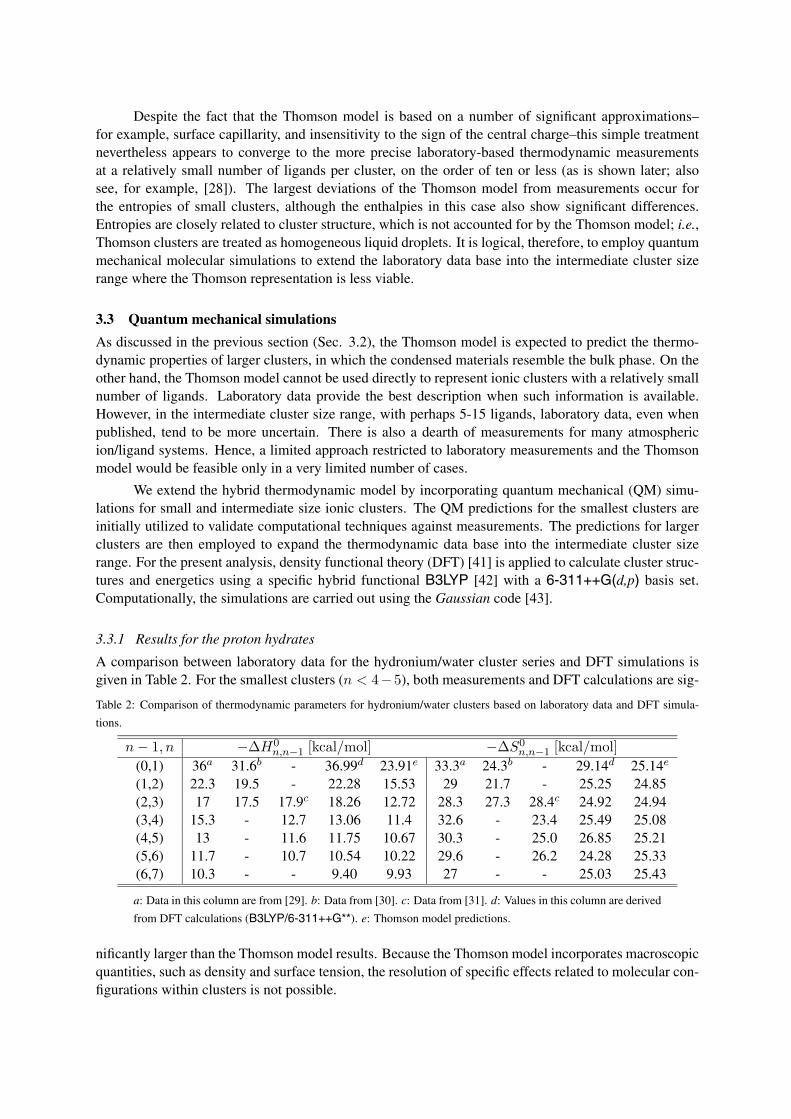
Despite the fact that the Thomson model is based on a number of significant approximations–for example, surface capillarity, and insensitivity to the sign of the central charge–this simple treatmentnevertheless appears to converge to the more precise laboratory-based thermodynamic measurementsat a relatively small number of ligands per cluster, on the order of ten or less (as is shown later; alsosee, for example, [28]). The largest deviations of the Thomson model from measurements occur forthe entropies of small clusters, although the enthalpies in this case also show significant differences.Entropies are closely related to cluster structure, which is not accounted for by the Thomson model; i.e.,Thomson clusters are treated as homogeneous liquid droplets. It is logical, therefore, to employ quantummechanical molecular simulations to extend the laboratory data base into the intermediate cluster sizerange where the Thomson representation is less viable.

3.3 Quantum mechanical simulations

As discussed in the previous section (Sec. 3.2), the Thomson model is expected to predict the thermo-dynamic properties of larger clusters, in which the condensed materials resemble the bulk phase. On theother hand, the Thomson model cannot be used directly to represent ionic clusters with a relatively smallnumber of ligands. Laboratory data provide the best description when such information is available.However, in the intermediate cluster size range, with perhaps 5-15 ligands, laboratory data, even whenpublished, tend to be more uncertain. There is also a dearth of measurements for many atmosphericion/ligand systems. Hence, a limited approach restricted to laboratory measurements and the Thomsonmodel would be feasible only in a very limited number of cases.

We extend the hybrid thermodynamic model by incorporating quantum mechanical (QM) simu-lations for small and intermediate size ionic clusters. The QM predictions for the smallest clusters areinitially utilized to validate computational techniques against measurements. The predictions for largerclusters are then employed to expand the thermodynamic data base into the intermediate cluster sizerange. For the present analysis, density functional theory (DFT) [41] is applied to calculate cluster struc-tures and energetics using a specific hybrid functional B3LYP [42] with a 6-311++G(d,p) basis set.Computationally, the simulations are carried out using the Gaussian code [43].

3.3.1 Results for the proton hydrates

A comparison between laboratory data for the hydronium/water cluster series and DFT simulations isgiven in Table 2. For the smallest clusters (n < 4−5), both measurements and DFT calculations are sig-

Table 2: Comparison of thermodynamic parameters for hydronium/water clusters based on laboratory data and DFT simula-

tions.

n − 1, n −∆H0n,n−1 [kcal/mol] −∆S0

n,n−1 [kcal/mol](0,1) 36a 31.6b - 36.99d 23.91e 33.3a 24.3b - 29.14d 25.14e

(1,2) 22.3 19.5 - 22.28 15.53 29 21.7 - 25.25 24.85(2,3) 17 17.5 17.9c 18.26 12.72 28.3 27.3 28.4c 24.92 24.94(3,4) 15.3 - 12.7 13.06 11.4 32.6 - 23.4 25.49 25.08(4,5) 13 - 11.6 11.75 10.67 30.3 - 25.0 26.85 25.21(5,6) 11.7 - 10.7 10.54 10.22 29.6 - 26.2 24.28 25.33(6,7) 10.3 - - 9.40 9.93 27 - - 25.03 25.43

a: Data in this column are from [29]. b: Data from [30]. c: Data from [31]. d: Values in this column are derived

from DFT calculations (B3LYP/6-311++G**). e: Thomson model predictions.

nificantly larger than the Thomson model results. Because the Thomson model incorporates macroscopicquantities, such as density and surface tension, the resolution of specific effects related to molecular con-figurations within clusters is not possible.

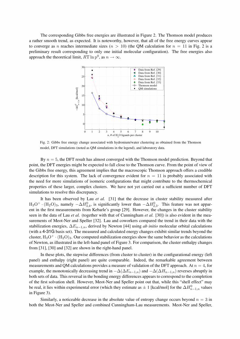
The corresponding Gibbs free energies are illustrated in Figure 2. The Thomson model producesa rather smooth trend, as expected. It is noteworthy, however, that all of the free energy curves appearto converge as n reaches intermediate sizes (n > 10) (the QM calculation for n = 11 in Fig. 2 is apreliminary result corresponding to only one initial molecular configuration). The free energies alsoapproach the theoretical limit, RT ln p0, as n → ∞.

0 1 2 3 4 5 6 7 8 9 10

0

5

10

15

20

25

30

n, # of H2O ligands per cluster

−DG

0 n−1,

n [kc

al/m

ol]

Data from Ref. [29]Data from Ref. [30]Data from Ref. [31]Data from Ref. [32]Data from Ref. [33]Thomson model QM simulations

Fig. 2: Gibbs free energy change associated with hydronium/water clustering as obtained from the Thomson

model, DFT simulations (noted as QM simulations in the legend), and laboratory data.

By n = 5, the DFT result has almost converged with the Thomson model prediction. Beyond thatpoint, the DFT energies might be expected to fall close to the Thomson curve. From the point of view ofthe Gibbs free energy, this agreement implies that the macroscopic Thomson approach offers a credibledescription for this system. The lack of convergence evident for n = 11 is probably associated withthe need for more simulations of isomeric configurations that might contribute to the thermochemicalproperties of these larger, complex clusters. We have not yet carried out a sufficient number of DFTsimulations to resolve this discrepancy.

It has been observed by Lau et al. [31] that the decrease in cluster stability measured afterH3O+ · (H2O)3, namely −∆H0

3,4, is significantly lower than −∆H02,3. This feature was not appar-

ent in the first measurements from Kebarle’s group [29]. However, the changes in the cluster stabilityseen in the data of Lau et al. (together with that of Cunningham et al. [30]) is also evident in the mea-surements of Meot-Ner and Speller [32]. Lau and coworkers compared the trend in their data with thestabilization energies, ∆En−1,n, derived by Newton [44] using ab initio molecular orbital calculations(with a 4-31G basis set). The measured and calculated energy changes exhibit similar trends beyond thecluster, H3O+ · (H2O)3. Our computed stabilization energies show the same behavior as the calculationsof Newton, as illustrated in the left-hand panel of Figure 3. For comparison, the cluster enthalpy changesfrom [31], [30] and [32] are shown in the right-hand panel.

In these plots, the stepwise differences (from cluster to cluster) in the configurational energy (leftpanel) and enthalpy (right panel) are quite comparable. Indeed, the remarkable agreement betweenmeasurements and QM calculations provides a measure of validation of the DFT approach. At n = 4, forexample, the monotonically decreasing trend in −∆(∆En−1,n) and −∆(∆Hn−1,n) reverses abruptly inboth sets of data. This reversal in the bonding energy differences appears to correspond to the completionof the first solvation shell. However, Meot-Ner and Speller point out that, while this “shell effect” maybe real, it lies within experimental error (which they estimate as ± 1 [kcal/mol] for the ∆H0

n−1,n valuesin Figure 3).

Similarly, a noticeable decrease in the absolute value of entropy change occurs beyond n = 3 inboth the Meot-Ner and Speller and combined Cunningham-Lau measurements. Meot-Ner and Speller,

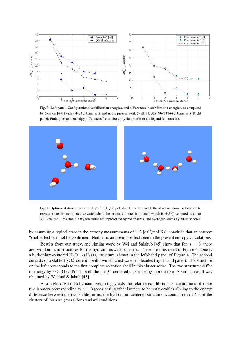
0 1 2 3 4 5 6 70

4

8

12

16

20

24

28

32

36

40

n, # of H2O ligands per cluster

−DE

n−1,

n [kc

al/m

ol]

From Ref. [44]QM simulations

0 1 2 3 4 5 6 70

5

10

15

20

25

30

35

40

n, # of H2O ligands per cluster

−DH

0 n−1,

n [kc

al/m

ol]

Data from Ref. [30]Data from Ref. [31]Data from Ref. [32]

Fig. 3: Left panel: Configurational stabilization energies, and differences in stabilization energies, as computed

by Newton [44] (with a 4-31G basis set), and in the present work (with a B3LYP/6-311++G basis set). Right

panel: Enthalpies and enthalpy differences from laboratory data (refer to the legend for sources).

Fig. 4: Optimized structures for the H3O+ · (H2O)3 cluster. In the left panel, the structure shown is believed to

represent the first completed solvation shell; the structure in the right panel, which is H5O+2 -centered, is about

3.3 [kcal/mol] less stable. Oxygen atoms are represented by red spheres, and hydrogen atoms by white spheres.

by assuming a typical error in the entropy measurements of ± 2 [cal/(mol·K)], conclude that an entropy“shell effect” cannot be confirmed. Neither is an obvious effect seen in the present entropy calculations.

Results from our study, and similar work by Wei and Salahub [45] show that for n = 3, thereare two dominant structures for the hydronium/water clusters. These are illustrated in Figure 4. One isa hydronium-centered H3O+ · (H2O)3 structure, shown in the left-hand panel of Figure 4. The secondconsists of a stable H5O+

2 core ion with two attached water molecules (right-hand panel). The structureon the left corresponds to the first complete solvation shell in this cluster series. The two structures differin energy by ∼ 3.3 [kcal/mol], with the H3O+-centered cluster being more stable. A similar result wasobtained by Wei and Salahub [45].

A straightforward Boltzmann weighting yields the relative equilibrium concentrations of thesetwo isomers corresponding to n = 3 (considering other isomers to be unfavorable). Owing to the energydifference between the two stable forms, the hydronium-centered structure accounts for ≈ 95% of theclusters of this size (mass) for standard conditions.

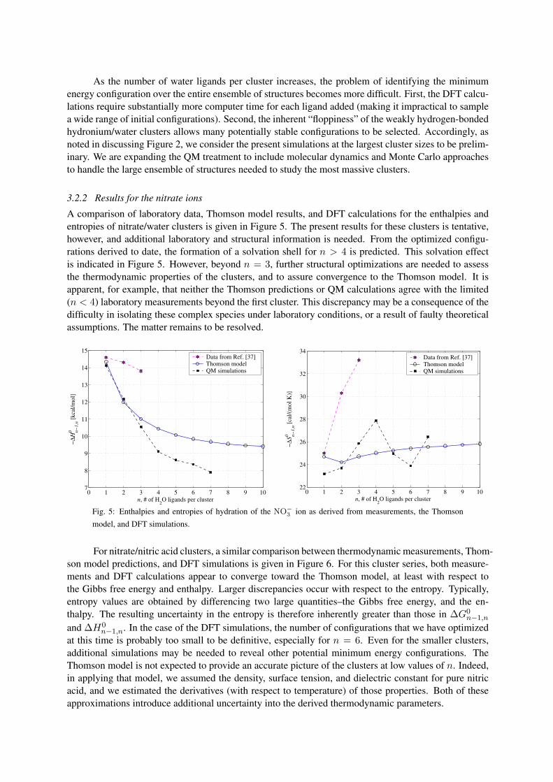
As the number of water ligands per cluster increases, the problem of identifying the minimumenergy configuration over the entire ensemble of structures becomes more difficult. First, the DFT calcu-lations require substantially more computer time for each ligand added (making it impractical to samplea wide range of initial configurations). Second, the inherent “floppiness” of the weakly hydrogen-bondedhydronium/water clusters allows many potentially stable configurations to be selected. Accordingly, asnoted in discussing Figure 2, we consider the present simulations at the largest cluster sizes to be prelim-inary. We are expanding the QM treatment to include molecular dynamics and Monte Carlo approachesto handle the large ensemble of structures needed to study the most massive clusters.

3.2.2 Results for the nitrate ions

A comparison of laboratory data, Thomson model results, and DFT calculations for the enthalpies andentropies of nitrate/water clusters is given in Figure 5. The present results for these clusters is tentative,however, and additional laboratory and structural information is needed. From the optimized configu-rations derived to date, the formation of a solvation shell for n > 4 is predicted. This solvation effectis indicated in Figure 5. However, beyond n = 3, further structural optimizations are needed to assessthe thermodynamic properties of the clusters, and to assure convergence to the Thomson model. It isapparent, for example, that neither the Thomson predictions or QM calculations agree with the limited(n < 4) laboratory measurements beyond the first cluster. This discrepancy may be a consequence of thedifficulty in isolating these complex species under laboratory conditions, or a result of faulty theoreticalassumptions. The matter remains to be resolved.

0 1 2 3 4 5 6 7 8 9 107

8

9

10

11

12

13

14

15

n, # of H2O ligands per cluster

−DH

0 n−1,

n [kc

al/m

ol]

Data from Ref. [37]Thomson model QM simulations

0 1 2 3 4 5 6 7 8 9 1022

24

26

28

30

32

34

n, # of H2O ligands per cluster

−DS

0 n−1,

n [ca

l/(m

olK

)]

Data from Ref. [37]Thomson model QM simulations

Fig. 5: Enthalpies and entropies of hydration of the NO−3 ion as derived from measurements, the Thomson

model, and DFT simulations.

For nitrate/nitric acid clusters, a similar comparison between thermodynamic measurements, Thom-son model predictions, and DFT simulations is given in Figure 6. For this cluster series, both measure-ments and DFT calculations appear to converge toward the Thomson model, at least with respect tothe Gibbs free energy and enthalpy. Larger discrepancies occur with respect to the entropy. Typically,entropy values are obtained by differencing two large quantities–the Gibbs free energy, and the en-thalpy. The resulting uncertainty in the entropy is therefore inherently greater than those in ∆G0

n−1,n

and ∆H0n−1,n. In the case of the DFT simulations, the number of configurations that we have optimized

at this time is probably too small to be definitive, especially for n = 6. Even for the smaller clusters,additional simulations may be needed to reveal other potential minimum energy configurations. TheThomson model is not expected to provide an accurate picture of the clusters at low values of n. Indeed,in applying that model, we assumed the density, surface tension, and dielectric constant for pure nitricacid, and we estimated the derivatives (with respect to temperature) of those properties. Both of theseapproximations introduce additional uncertainty into the derived thermodynamic parameters.

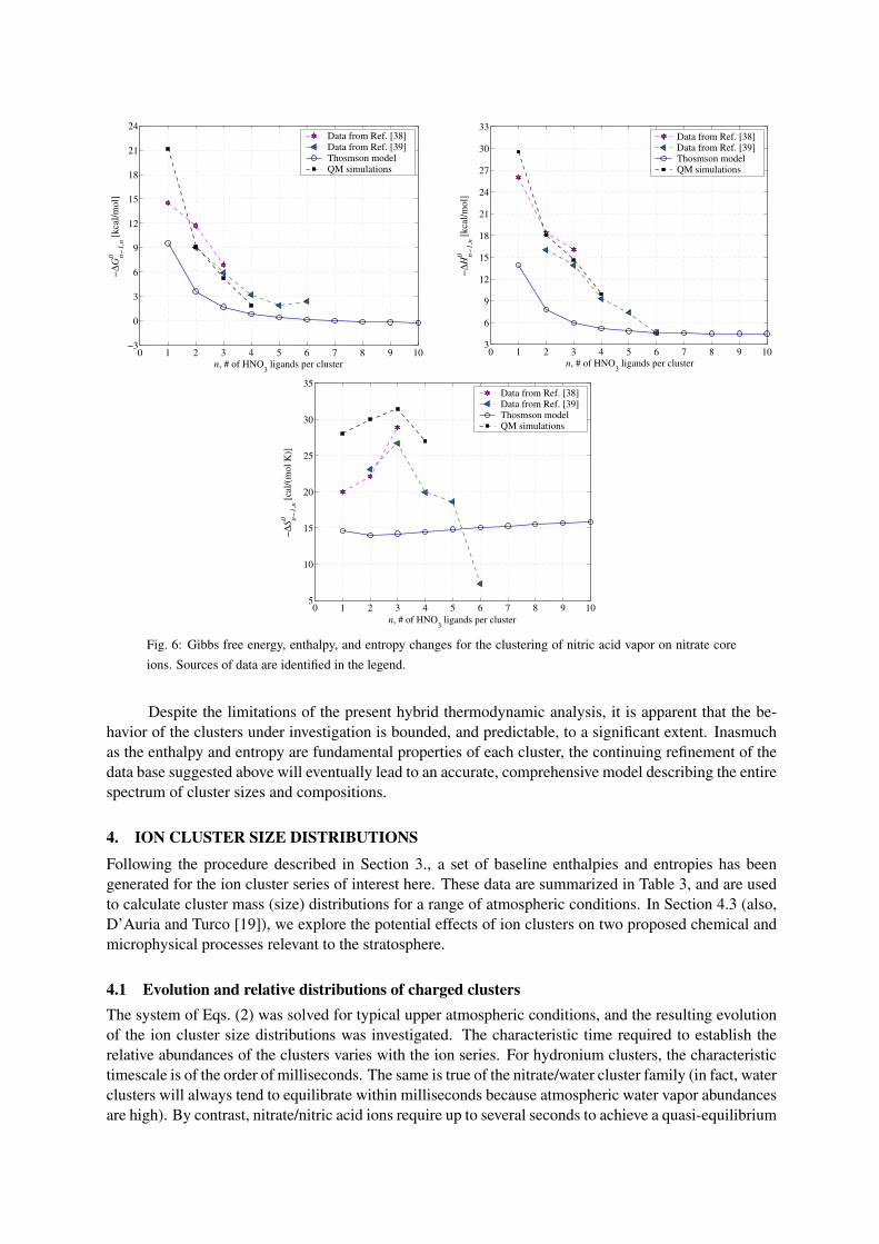
0 1 2 3 4 5 6 7 8 9 10−3

0

3

6

9

12

15

18

21

24

n, # of HNO3 ligands per cluster

−DG

0 n−1,

n [kc

al/m

ol]

Data from Ref. [38]Data from Ref. [39]Thosmson model QM simulations

0 1 2 3 4 5 6 7 8 9 103

6

9

12

15

18

21

24

27

30

33

n, # of HNO3 ligands per cluster

−DH

0 n−1,

n [kc

al/m

ol]

Data from Ref. [38]Data from Ref. [39]Thosmson model QM simulations

0 1 2 3 4 5 6 7 8 9 105

10

15

20

25

30

35

n, # of HNO3 ligands per cluster

−DS

0 n−1,

n [ca

l/(m

olK

)]

Data from Ref. [38]Data from Ref. [39]Thosmson model QM simulations

Fig. 6: Gibbs free energy, enthalpy, and entropy changes for the clustering of nitric acid vapor on nitrate core

ions. Sources of data are identified in the legend.

Despite the limitations of the present hybrid thermodynamic analysis, it is apparent that the be-havior of the clusters under investigation is bounded, and predictable, to a significant extent. Inasmuchas the enthalpy and entropy are fundamental properties of each cluster, the continuing refinement of thedata base suggested above will eventually lead to an accurate, comprehensive model describing the entirespectrum of cluster sizes and compositions.

4. ION CLUSTER SIZE DISTRIBUTIONS

Following the procedure described in Section 3., a set of baseline enthalpies and entropies has beengenerated for the ion cluster series of interest here. These data are summarized in Table 3, and are usedto calculate cluster mass (size) distributions for a range of atmospheric conditions. In Section 4.3 (also,D’Auria and Turco [19]), we explore the potential effects of ion clusters on two proposed chemical andmicrophysical processes relevant to the stratosphere.

4.1 Evolution and relative distributions of charged clusters

The system of Eqs. (2) was solved for typical upper atmospheric conditions, and the resulting evolutionof the ion cluster size distributions was investigated. The characteristic time required to establish therelative abundances of the clusters varies with the ion series. For hydronium clusters, the characteristictimescale is of the order of milliseconds. The same is true of the nitrate/water cluster family (in fact, waterclusters will always tend to equilibrate within milliseconds because atmospheric water vapor abundancesare high). By contrast, nitrate/nitric acid ions require up to several seconds to achieve a quasi-equilibrium

Table 3: Standard enthalpies and entropies for the addition of a ligand in the cluster sequences indicated, up to the first 10

ligands in each sequence.

H3O+ · (H2O)an NO−

3 · (H2O)bn NO−

3 · (HNO3)cn

n − 1, n −∆H0n−1,n −∆S0

n−1,n −∆H0n−1,n −∆S0

n−1,n −∆H0n−1,n −∆S0

n−1,n

[kcal/mol] [cal/mol·K] [kcal/mol] [cal/mol·K] [kcal/mol] [cal/mol·K]0,1 36 33.3 14.6 25.0 26.0 ≥20.1,2 22.3 29 14.3 30.3 16.0 23.12,3 17 28.3 13.8 33.2 13.9 26.73,4 15.3 32.6 10.4 25.0 9.3 19.94,5 13 30.3 10.1 25.2 7.4 18.65,6 11.7 29.6 9.8 25.4 4.6 15.1 (7.3)†

6,7 10.3 27 9.7 25.5 4.5 15.37,8 9.7 25.5 9.6 25.6 4.5 15.58,9 9.6 25.6 9.5 25.6 4.5 15.7

9,10 9.5 25.7 9.4 25.6 4.5 15.8

a: For H3O+ · (H2O)n: n = 1, · · · , 7 data are from [29], and for n > 7 from the Thomson model. Other data

from [30] and [31] are used for sensitivity analysis. b: For NO−3 · (H2O)n: n = 1, · · · , 3 data are from [37],

and for n > 3 from the Thomson model. c: For NO−3 · (HNO3)n: data are from [38] for n = 1, from [39]

for n = 2, · · · , 6, and from the Thomson model for n > 6. †: The entropy value in brackets is from [39], but

is considered unreliable. Accordingly, the entropy predicted by the Thomson model is used for this cluster as

well.

mass distribution, owing to the lower amounts of nitric acid vapor in air. It is crucial to note, however,that in either case, the time required to establish the characteristic ion mass spectrum is much shorter thanthe ion-ion recombination lifetime, ∼ 300 s. This implies that distinct relative ion populations withincluster families will always exist in an air mass that is continuously ionized.

In Figure 7, typical size distributions are displayed for clusters of nitrate core ions with water(left panel) and with nitric acid (right panel). The relative nitrate/water cluster distribution reaches aquasi-equilibrium state in roughly 50 milliseconds, after which the spectrum of the predominant clustersremains fixed. The equilibration time for nitrate/nitric acid clusters is also fairly short–of the order ofseconds. While over the time scales indicated, the relative cluster distributions effectively reach a steady-state (identified by t = ∞ in the figure legend), the absolute cluster concentrations continue to build upover a much longer period, which is determined by the mean ion lifetime (roughly 300 s for conditionsrelevant to the lower stratosphere).

The most probable nitrate/water clusters are found to have about 6-10 ligands. This range varieswith the water vapor concentration and ambient temperature. By contrast, the nitrate/nitric acid clusterstypically have three ligands for the conditions tested. More water molecules are collected in part becausethe partial pressure of H2O is much greater than that of HNO3.

For ion nucleation, water clusters of critical size contain hundreds to thousands of ligands (fora range of typical stratospheric water vapor concentrations and environmental conditions). The criticalnumber is determined by the maximum in the Gibbs free energy change associated with cluster formation[26]. Figure 8 shows the free energy curves corresponding to the hydronium ion series at several specifictemperatures. For temperatures above 170 K, a distinct peak occurs in ∆G0,n (although the peak liesoff the chart for T > 175K). The number of ligands at this local peak defines the size of the criticalcluster (nucleation embryo), as indicated in the figure. Similarly, the local minimum in the free energydefines the most probably cluster size. That is, the most abundant ion clusters will lie within the freeenergy “well,” which is typically far removed from the critical cluster size. The difference between the

0 5 10 15 200

5

10

15

20

25

30

35

n, # of ligands per cluster

Fra

ctio

nal A

boun

danc

es [

%]

NO3−(H

2O) p = 100 mbar

n[H

2O] = 5 ppmv T = 175 K

t=.1 [ms]t=.2 [ms] t=.3 [ms] t=.4 [ms] t= 1 [ms] t=50[ms]t= ¥

2 4 6 8 100

10

20

30

40

50

60

70

80

90

100

110

120

130

Fra

ctio

nal A

boun

danc

es [

%]

NO3−(HNO

3) p = 100 mbarn

[HNO3] = 10 ppbv T = 175 K

t= 5 [ms] t=50 [ms]t=0.1 [s] t=0.2 [s] t=0.5 [s] t= 5 [s] t=¥

Fig. 7: Relative concentrations (in percent) of nitrate/water clusters (left panel) and nitrate/nitric acid clusters

(right panel) as a function of time, assuming the production of initially bare nitrate core ions, under the conditions

indicated in the legend. From D’Auria and Turco [19].

100

101

102

103

104

−100

−50

0

50

100

n, # of ligands per cluster

DG0,

n [kc

al/m

ol]

H3O+(H

2O)

np = 100 mbar

170 K

175 K

180 K

190 K

220 K

210 K

200 K

Fig. 8: Gibbs free energy changes for the formation of hydronium ion clusters with n water ligands. At each

temperature, the vertical dashed line corresponding to the local maximum in the free energy defines the size of

the critical cluster; the dashed line at the local minimum identifies the size of the most probable cluster.

energy maximum and energy minimum defines the energy “barrier” to nucleation. Notice that, as thetemperature decreases in Figure 8, the energy barrier is systematically lowered. If temperatures were tofall below ∼170 K, the barrier would disappear and the hydronium ions would nucleate freely. In thefigure, the size of the critical cluster increases dramatically as the temperature rises. At 175 K, morethan 400 water ligands would be needed to build a nucleation embryo. Because these cluster sizes areso large, and the corresponding cluster concentrations are so small, the nucleation of pure water ontohydronium ions will not occur in the lower stratosphere even in the most extreme situations.

Figure 9 summarizes the behavior of the three cluster families of interest for a wide range oftemperatures at 100 mbar, assuming 5 ppmv of water vapor and 10 ppbv of nitric acid vapor (as inprevious figures). As the temperature increases, the peak of each size distribution tends to shift towardsmaller cluster sizes. This is to be expected, inasmuch as higher temperatures create conditions lessfavorable to condensation. It is worth noting that at 180 K, roughly 10% of the hydrated hydronium andnitrate clusters have 10 or more ligands.

The nitrate/nitric acid clusters are much smaller (in terms of the number of ligands, not necessarilymass), even at very low temperatures. It is likely, however, that these clusters will take up water fromthe environment and grow much larger (refer, for example, to the nitrate/water series). Among other

180 190 200 210 3

6

9

12

15

18

21

10

20

3040 50

60

10

20

30405070

170 180 190 200 210 220

T [K]

n, #

of

ligan

ds p

er c

lust

er

1050 80

80

20 60

1

2 3 4

NO3−(H

2O)

n+9

H3O+(H

2O)

n

NO3−(HNO

3) n

Fig. 9: Equilibrium cluster size distributions for three common series of atmospheric cluster ions. The plot is

divided into lower and upper panels, where the vertical scale (indicating the number of ligands) is linear in the

upper panel and logarithmic in the lower panel. Data are displayed as isopleths corresponding to the percentage

of the total number of ions in a family having a specific number of ligands, at each temperature. The cluster

series are identified in the figure: NO−3 · (H2O)n (upper contours in the top panel); H3O

+ · (H2O)n (lower

contours in the top panel); and NO−3 · (HNO3)n (contours in the lower panel). An offset of n = 9 ligands for

the nitrate/water clusters separates them from the hydronium/water ions. From D’Auria and Turco [19].

things, the vapor pressures above solutions of HNO3 and H2O are generally much lower than the vaporpressures over the pure substances, suggesting that such mixtures –even on microscopic scales–will bemore stable.

Information on mixed water/nitric acid cluster ions is sparse. In one case, stratospheric mass spec-trometric data were used to infer the free energy for the (1,1) nitrate-based H2O/HNO3 cluster [46].Larger negatively-charged mixed ion clusters have not been detected under midlatitude conditions. Like-wise, nitric acid attached to ambient hydronium clusters has not been reported. However, Castlemanand co-workers have carried out studies of water/nitric acid clusters formed around hydronium core ions(e.g., [47], [48], [49]). They found that nitric acid is readily taken up by ions (of both signs) containing asufficient number of water ligands (typically four for the first nitric acid ligand, eight for the second, andsomewhat fewer water molecules per additional HNO3 ligand). These investigations suggest minimumfree energies for clusters having H2O/HNO3 molar ratios approaching that of the nitric acid trihydrateice (i.e., 3:1), although the data are currently incomplete. We are currently simulating the properties ofmixed H2O/HNO3 nitrate and hydronium clusters of the type studied by Castleman et al. to extend theirresults.

In the polar winter stratosphere, where sufficiently low temperatures are reached, newly formedhydronium and nitrate core ions may quickly become hydrated with 10 or more water molecules (Fig. 9).Some ions may collect many more. The largest water clusters would readily take up nitric acid vapor, ashas been noted experimentally. At temperatures approaching 195 K, perhaps 2-3 nitric acid moleculeswould initially condense on the largest hydrated ions, further stabilizing these species. As temperaturesdropped below 195 K, additional HNO3 and H2O would be taken up. Even a relatively small populationof charged clusters with 5-6 HNO3 molecules (and many more H2O ligands) constitutes a potentially im-portant source of freezing nuclei at temperatures in the vicinity of 190 K [18]. At the lowest temperaturesattainable, it is not inconceivable that some of the largest clusters would nucleate into new aerosols.

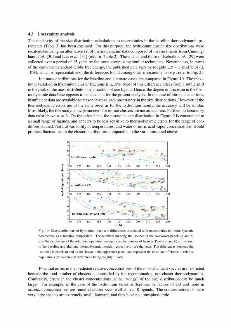
4.2 Uncertainty analysis

The sensitivity of the size distribution calculations to uncertainties in the baseline thermodynamic pa-rameters (Table 3) has been explored. For this purpose, the hydronium cluster size distributions wererecalculated using an alternative set of thermodynamic data composed of measurements from Cunning-ham et al. [30] and Lau et al. [31] (refer to Table 2). These data, and those of Kebarle et al. [29] werecollected over a period of 15 years by the same group using similar techniques. Nevertheless, in termsof the equivalent standard Gibbs free energy, the published data vary by roughly ±2 − 3 kcal/mol (±10%), which is representative of the differences found among other measurements (e.g., refer to Fig. 2).

Ion mass distributions for the baseline and alternate cases are compared in Figure 10. The maxi-mum variation in hydronium cluster fractions is ±15%. Most of this difference arises from a subtle shiftin the peak of the mass distribution by a fraction of one ligand. Hence, the degree of precision in the ther-modynamic data base appears to be adequate for the present analysis. In the case of nitrate cluster ions,insufficient data are available to reasonably evaluate uncertainty in the size distributions. However, if thethermodynamic errors are of the same order as for the hydronium family, the accuracy will be similar.Most likely, the thermodynamic parameters for nitrate clusters are not as accurate. Further, no laboratorydata exist above n = 6. On the other hand, the nitrate cluster distribution in Figure 9 is constrained toa small range of ligands, and appears to be less sensitive to thermodynamic errors for the range of con-ditions studied. Natural variability in temperatures, and water or nitric acid vapor concentrations, wouldproduce fluctuations in the cluster distributions comparable to the variations cited above.

170 175 180 185 190 195 200 205 210 215 2203

4

5

6

7

8

−15

−10−10

−10−10

−5

−5−5

−5

−5

0

00

0

5

55

5

510

1010 15

170 175 180 185 190 195 200 205 210 215 2203

4

5

6

7

8

n, #

of

ligan

ds p

er c

lust

er

0

10

10

10

10

10

20

20

20

20

20

30

30

30

30

30

30

40

4040

40

40

5050

50

5050

6060

170 175 180 185 190 195 200 205 210 215 2203

4

5

6

7

8

T [K]

10

10

10

10

10

10

20

20

20

20

20

30

30

30

30

30

404040

40

4050

5050

506060

b) with Ref. [29] and [30]

a) with Ref. [28]

% difference a)−b)

Fig. 10: Size distributions of hydronium ions, and differences associated with uncertainties in thermodynamic

parameters, as a function temperature. The numbers marking the isolines in the two lower panels (a and b)

give the percentage of the total ion population having a specific number of ligands. Panels a) and b) correspond

to the baseline and alternate thermodynamic models, respectively (see the text). The differences between the

isopleths in panels a) and b) are shown in the uppermost panel, and represent the absolute difference in relative

populations (the maximum differences being roughly ±15%.

Potential errors in the predicted relative concentrations of the most abundant species are restrictedbecause the total number of clusters is controlled by ion recombination, not cluster thermodynamics.Conversely, errors in the cluster concentrations in the “wings” of the size distribution can be muchlarger. For example, in the case of the hydronium series, differences by factors of 2-3 and more inabsolute concentrations are found at cluster sizes well above 10 ligands. The concentrations of thesevery large species are extremely small, however, and they have no atmospheric role.

4.3 Polar processes

Using the model described above, we can explore the role of ionic clusters in stratospheric chemistry andmicrophysics. Kawa and coworkers [50] have suggested that the decomposition of N2O5 on hydratedcluster ions is a source of nitric acid in the polar winter stratosphere. To test this hypothesis, the presentthermodynamic/kinetic model can be applied to estimate the rates of cluster-induced heterogeneous de-composition of N2O5 at 40 km. Hamill and Turco [18] proposed that hydrated nitrate/nitric acid clustersmay act as freezing nuclei when they impinge on supercooled polar stratospheric cloud (PSC) particles.In this case, the collision frequencies of NO−

3 · (HNO3)n cluster ions with preexisting supercooled PSCdroplets can be calculated using the model developed here.

4.3.1 Heterogeneous conversion of N2O5

The rate of reaction of N2O5 with proton hydrates may be quantified using hydronium ion mass distribu-tions corresponding to the environmental conditions encountered at 40 km (i.e, ∼ 3 mbar and ∼ 250 K).These distributions are easily derived using our hybrid ion cluster model. The results are displayed inFig. 11 for both the baseline and alternate thermodynamic data sets utilized in previous sections.

0 1 2 3 4 5 60

10

20

30

40

50

60

70

80

90

100

n, # of ligands per cluster

(C(n

,t)/S

n=0

NC

(n,t)

) [%

]

a)

t=0.1 [ms]t=0.2 [ms]t=0.3 [ms]t=0.4 [ms]t=1 [ms] t=50 [ms] t=¥

0 1 2 3 4 5 6 70

10

20

30

40

50

60

70

80

90

100

n, # of ligands per cluster

(C(n

,t)/S

n=0

NC

(n,t)

) [%

]

b)

t=0.1 [ms]t=0.2 [ms]t=0.3 [ms]t=0.4 [ms]t=1 [ms] t=50 [ms] t=¥

Fig. 11: Stratospheric hydronium water cluster size distributions. Panel a): relative concentrations correspond-

ing to the baseline thermodynamic data in Table 3 ([29]); Panel b): concentrations corresponding to the ther-

modynamic data from [30] and [31]. In both cases, ambient conditions at an altitude of ∼ 40 km are assumed.

Rate coefficients for the reaction of N2O5 with hydronium-based ions have been reported byBohringer and coworkers [51] for the first 6 hydrated species. Because the cluster concentrations forn > 6 are negligible (Fig. 11), rate coefficients for these massive ions are not required. However, onlyupper-limit rate constants are specified for ions having 3 or more water ligands. It follows that the derivedloss rates for the decomposition of N2O5 on proton hydrates will represent upper limits for this process.

Combining the modeled cluster ion size distribution with the known reaction rate coefficients, theoverall loss rate for N2O5 is found to be less than 3 × 10−8 s−1. This upper limit applies to both ofthe cluster size distributions in Figure 11. The fastest reactions between N2O5 and the proton hydratesoccur for the smallest clusters, with n < 3. On the other hand, PH clusters in the middle stratosphereare dominated by hydronium with three water ligands. Consequently, the overall reaction efficiency ofN2O5 with such clusters is quite low–in fact, two orders of magnitude too low to influence the behaviorof odd-nitrogen in the stratosphere.

4.3.2 Ion cluster interactions with PSCs

Hamill and Turco [18] recently suggested that nitrate ion clusters having a composition similar to that ofthe nitric acid trihydrate may act as freezing nuclei for type 1b PSC particles consisting of supercooled

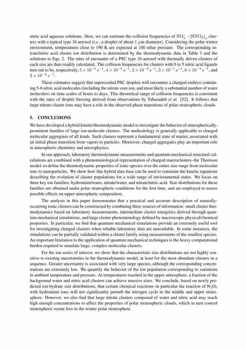
nitric acid aqueous solutions. Here, we can estimate the collision frequencies of NO−3 · (HNO3)n clus-

ters with a typical type 1b aerosol (i.e., a droplet of about 1 µm diameter). Considering the polar winterenvironment, temperatures close to 190 K are expected at 100 mbar pressure. The corresponding ni-trate/nitric acid cluster ion distribution is determined by the thermodynamic data in Table 3 and thesolutions to Eqs. 2. The rates of encounter of a PSC type 1b aerosol with thermally driven clusters ofeach size are then readily calculated. The collision frequencies for clusters with 0 to 5 nitric acid ligandsturn out to be, respectively, 5× 10−5 s−1, 4× 10−5 s−1, 2× 10−2 s−1, 3× 10−1 s−1, 6× 10−4 s−1, and2 × 10−8 s−1.

These estimates suggest that supercooled PSC droplets will encounter a charged embryo contain-ing 5-6 nitric acid molecules (including the nitrate core ion, and most likely a substantial number of watermolecules) on time scales of hours to days. This theoretical range of collision frequencies is consistentwith the rates of droplet freezing derived from observations by Tabazadeh et al. [52]. It follows thatlarge nitrate cluster ions may have a role in the observed phase transitions of polar stratospheric clouds.

5. CONCLUSIONS

We have developed a hybrid kinetic/thermodynamic model to investigate the behavior of atmospherically-prominent families of large ion-molecule clusters. The methodology is generally applicable to chargedmolecular aggregates of all kinds. Such clusters represent a fundamental state of matter, associated withan initial phase transition from vapors to particles. Moreover, charged aggregates play an important rolein atmospheric chemistry and microphysics.

In our approach, laboratory thermodynamic measurements and quantum mechanical structural cal-culations are combined with a phenomenological representation of charged macroclusters–the Thomsonmodel–to define the thermodynamic properties of ionic species over the entire size range from molecularions to nanoparticles. We show how this hybrid data base can be used to constrain the kinetic equationsdescribing the evolution of cluster populations for a wide range of environmental states. We focus onthree key ion families; hydronium/water, nitrate/water, and nitrate/nitric acid. Size distributions for thesefamilies are obtained under polar stratospheric conditions for the first time, and are employed to assesspossible effects on upper-atmospheric composition.

The analysis in this paper demonstrates that a practical and accurate description of naturally-occurring ionic clusters can be constructed by combining three sources of information: small cluster ther-modynamics based on laboratory measurements, intermediate cluster energetics derived through quan-tum mechanical simulations, and large cluster phenomenology defined by macroscopic physical/chemicalproperties. In particular, we find that quantum mechanical simulations provide an extremely useful toolfor investigating charged clusters when reliable laboratory data are unavailable. In some instances, thesimulations can be partially validated within a cluster family using measurements of the smallest species.An important limitation to the application of quantum mechanical techniques is the heavy computationalburden required to simulate large, complex molecular clusters.

For the ion series of interest, we show that the characteristic size distributions are not highly sen-sitive to existing uncertainties in the thermodynamic model, at least for the most abundant clusters in asequence. Greater uncertainty is associated with very large species, although the corresponding concen-trations are extremely low. We quantify the behavior of the ion population corresponding to variationsin ambient temperature and pressure. At temperatures reached in the upper atmosphere, a fraction of thebackground water and nitric acid clusters can achieve massive sizes. We conclude, based on newly pre-dicted ion-hydrate size distributions, that certain chemical reactions–in particular the reaction of N2O5

with hydronium ions–will not significantly perturb the nitrogen cycle in the middle and upper strato-sphere. However, we also find that large nitrate clusters composed of water and nitric acid may reachhigh enough concentrations to affect the properties of polar stratospheric clouds, which in turn controlstratospheric ozone loss in the winter polar stratosphere.

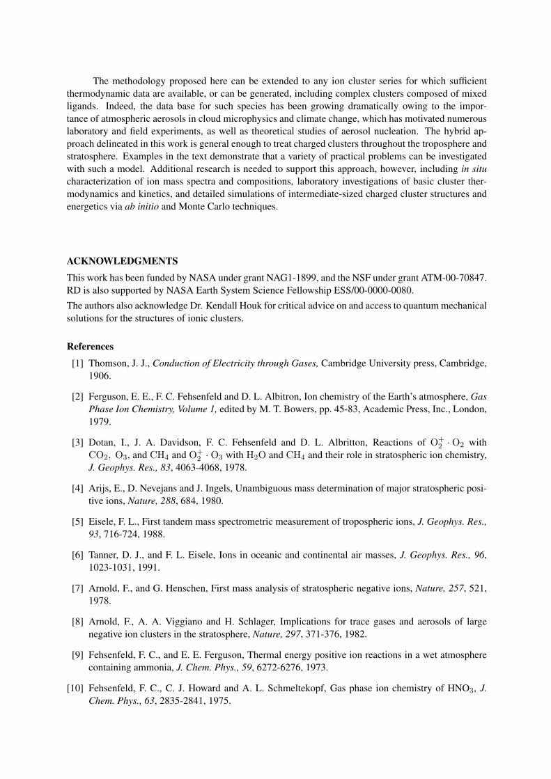
The methodology proposed here can be extended to any ion cluster series for which sufficientthermodynamic data are available, or can be generated, including complex clusters composed of mixedligands. Indeed, the data base for such species has been growing dramatically owing to the impor-tance of atmospheric aerosols in cloud microphysics and climate change, which has motivated numerouslaboratory and field experiments, as well as theoretical studies of aerosol nucleation. The hybrid ap-proach delineated in this work is general enough to treat charged clusters throughout the troposphere andstratosphere. Examples in the text demonstrate that a variety of practical problems can be investigatedwith such a model. Additional research is needed to support this approach, however, including in situcharacterization of ion mass spectra and compositions, laboratory investigations of basic cluster ther-modynamics and kinetics, and detailed simulations of intermediate-sized charged cluster structures andenergetics via ab initio and Monte Carlo techniques.

ACKNOWLEDGMENTS

This work has been funded by NASA under grant NAG1-1899, and the NSF under grant ATM-00-70847.RD is also supported by NASA Earth System Science Fellowship ESS/00-0000-0080.

The authors also acknowledge Dr. Kendall Houk for critical advice on and access to quantum mechanicalsolutions for the structures of ionic clusters.

References

[1] Thomson, J. J., Conduction of Electricity through Gases, Cambridge University press, Cambridge,1906.

[2] Ferguson, E. E., F. C. Fehsenfeld and D. L. Albitron, Ion chemistry of the Earth’s atmosphere, GasPhase Ion Chemistry, Volume 1, edited by M. T. Bowers, pp. 45-83, Academic Press, Inc., London,1979.

[3] Dotan, I., J. A. Davidson, F. C. Fehsenfeld and D. L. Albritton, Reactions of O+2 · O2 with

CO2, O3, and CH4 and O+2 · O3 with H2O and CH4 and their role in stratospheric ion chemistry,

J. Geophys. Res., 83, 4063-4068, 1978.

[4] Arijs, E., D. Nevejans and J. Ingels, Unambiguous mass determination of major stratospheric posi-tive ions, Nature, 288, 684, 1980.

[5] Eisele, F. L., First tandem mass spectrometric measurement of tropospheric ions, J. Geophys. Res.,93, 716-724, 1988.

[6] Tanner, D. J., and F. L. Eisele, Ions in oceanic and continental air masses, J. Geophys. Res., 96,1023-1031, 1991.

[7] Arnold, F., and G. Henschen, First mass analysis of stratospheric negative ions, Nature, 257, 521,1978.

[8] Arnold, F., A. A. Viggiano and H. Schlager, Implications for trace gases and aerosols of largenegative ion clusters in the stratosphere, Nature, 297, 371-376, 1982.

[9] Fehsenfeld, F. C., and E. E. Ferguson, Thermal energy positive ion reactions in a wet atmospherecontaining ammonia, J. Chem. Phys., 59, 6272-6276, 1973.

[10] Fehsenfeld, F. C., C. J. Howard and A. L. Schmeltekopf, Gas phase ion chemistry of HNO3, J.Chem. Phys., 63, 2835-2841, 1975.

[11] Davidson, J. A., F. C. Fehsenfeld and C. J. Howard, The heats of formation of NO−3 and NO−

3

association complexes with HNO3 and HBr, Int. J. Chem. Kinet., 9, 17-29, 1977.

[12] Brasseur, G., and A. Chatel, Modelling of stratospheric ions: A first attempt, Ann. Geophys., 1,149-160, 1983.

[13] Kawamoto, H., and T. Ogawa, A steady state of negative ions in the lower stratosphere, Planet.Space Sci., 32, 1223-1233, 1984.

[14] Kawamoto, H., and T. Ogawa, First model of negative ion composition in the troposphere, Planet.Space Sci., 34, 1229-1239, 1986.

[15] Beig, G., S. Walters and G. Brasseur, A two-dimensional model of ion composition in thestratosphere-1. Positive ions, J. Geophys. Res., 98, 12,767-12,773, 1993.

[16] Beig, G., and G. Brasseur, Model of tropospheric ion composition: A first attempt, J. Geophys.Res., 105, 22,671-22,684, 2000.

[17] Viggiano, A. A., F. Dale and J. F. Paulson, Proton transfer reactions of H+ · (H2O)n=2,11 withmethanol, ammonia, pyridine, acetonitrile, and acetone, J. Chem. Phys., 88, 2469-2477, 1987.

[18] Hamill P., and R. P. Turco, Ion nucleation of NAT in ternary system polar stratospheric clouds,Trans. Amer. Geophys. Union, 81 (#19, May 9, 2000) Suppl., S97, 2000.

[19] D’Auria, R., and R. P. Turco, Ionic clusters in the polar winter stratosphere, Geophys. Res. Lett., inpress, 2001.

[20] Zhao, J., O. B. Toon and R. P. Turco, Origin of condensation nuclei in the springtime polar strato-sphere, J. Geophys. Res., 100, 5215-5227, 1995.

[21] Bates, D. R., Recombination of small ions in the troposphere and lower stratosphere, Planet. SpaceSci., 30, 1275-1282, 1982.

[22] Cole, R. K., and E. T. Pierce, Electrification in the Earth’s atmosphere for altitudes between 0 and100 kilometers, J. Geophys. Res., 70, 2735-2749, 1965.

[23] Paltridge, G. W., Experimental measurements of the small-ion density and electrical conductivityof the stratosphere, J. Geophys. Res., 70, 2751,2761, 1965.

[24] Paltridge, G. W., Stratospheric small-ion density measurements from a high-altitude jet aircraft, J.Geophys. Res., 71, 1945-1952, 1966.

[25] Ferguson, E. E., Laboratory measurements of ionospheric ion-molecule reaction rates, Rev. Geo-phys., 12, 703-713, 1974.

[26] Castleman, A. W., Jr., and I. N. Tang, Role of small clusters in nucleation about ions, J. Chem.Phys., 57, 3629-3638, 1972.

[27] Castleman, A. W., Jr., P. M. Holland and R. G. Keesee, The properties of ion clusters and theirrelationship to heteromolecular nucleation, J. Chem. Phys., 68, 1760-1767, 1978.

[28] Holland, P. M., and A. W. Castleman, Jr., Thomson equation revisited in light of ion-clusteringexperiments, J. Phys. Chem., 86, 4181-4188, 1982.

[29] Kebarle, P., S. K. Searles, A. Zolla, J. Scarborough and M. Arshadi, The Solvation of the hydrogenion by water molecules in the gas phase. Heats and entropies of solvation of the individual reactions:H+(H2O)n−1 + H2O = H+(H2O)n, J. Am. Chem. Soc., 89, 6393-6399, 1967.

[30] Cunningham, A. J., J. D. Payzant and P. Kebarle, A kinetic study of the proton hydrate H+(H2O)n

equilibria in the gas phase, J. Am. Chem. Soc., 94, 7627-7632, 1972.

[31] Lau, Y. K., S. Ikuta and P. Kebarle, Thermodynamics and kinetics of the gas-phase reactions:H3O+(H2O)n−1 + H2O = H3O+(H2O)n, J. Am. Chem. Soc., 104, 1462-1469, 1982.

[32] Meot-Ner M., and C. V. Speller, The filling of solvents shells in cluster ions. 1. Thermochemicalcriteria and the effects of isomeric clusters, J. Phys. Chem., 90, 6616-6624, 1986.

[33] Shi, Z., J. V. Ford, S. Wei and A. W. Castleman, Jr., Water clusters: Contributions of binding energyand entropy to stability, J. Chem. Phys., 99, 8009-8015, 1993.

[34] Klots, C. E., Kinetic methods for quantifying magic (atomic clusters), Z. Phys. D 21, 335-342,1991.

[35] Yang, X., and A. W. Castleman, Jr., Large protonated water clusters H+(H2O)n (1 ≤ n > 60):The production and reactivity of clathrate-like structures under thermal conditions, J. Am. Chem.Soc., 111, 6845-6846, 1989.

[36] Magnera, T. F., D. E. David and J. Michl, The first twenty-eight gas-phase proton hydration ener-gies, Chem. Phys. Lett, 182, 363-370, 1991.

[37] Lee, N., R. G. Keesee and A. W. Castleman, Jr., The properties of clusters in the gas phase. IV.Complexes of H2O and HNOx clustering on NO−

x , J. Chem. Phys., 72, 1089-1094, 1980.

[38] Davidson, J. A., F. C. Fehsenfeld and C. J. Howard, The heats of formation of NO−3 and NO−

3

association complexes with HNO3 and HBr, Int. J. Chem. Kinet., 9, 17-29, 1977.

[39] Wlodek, S., Z. Luczynski and H. Wincel, Stabilities of gas-phase NO−3 · (HNO3)n, n ≤ 6, clusters,

Int. J. Mass Spectrom. Ion Phys., 35, 39-46,1980.

[40] Arnold, F., and S. Qiu, Upper stratosphere negative ion composition measurements and infraredtrace gas abundances, Planet. Space Sci., 32, 169-177, 1984.

[41] Kohn, W., and L. J. Sham, Self-consistent equations including exchange and correlation effects,Phys. Rev., 140A, 1133, 1965.

[42] Becke, A. D., A new mixing of Hartree-Fock and local density-functional theories, J. Chem. Phys.,98, 1372-1377, 1993.

[43] Frisch, M. J., G. W. Trucks, H. B. Schlegel, G. E. Scuseria, M. A. Robb, J. R. Cheeseman, V.G. Zakrzewski, J. A. Montgomery, R. E. Stratmann, J. C. Burant, S. Dapprich, J. M. Millam, A.D. Daniels, K. N. Kudin, M. C. Strain, O. Farkas, J. Tomasi, V. Barone, M. Cossi, R. Cammi, B.Mennucci, C. Pomelli, C. Adamo, S. Clifford, J. Ochterski, G. A. Petersson, P. Y. Ayala, Q. Cui,K. Morokuma, D. K. Malick, A. D. Rabuck, K. Raghavachari, J. B. Foresman, J. Cioslowski, J. V.Ortiz, B. B. Stefanov, G. Liu, A. Liashenko, P. Piskorz, I. Komaromi, R. Gomperts, R. L. Martin,D. J. Fox, T. Keith, M. A. Al-Laham, C. Y. Peng, A. Nanayakkara, C. Gonzalez, M. Challacombe,P. M. W. Gill, B. G. Johnson, W. Chen, M. W. Wong, J. L. Andres, M. Head-Gordon, E. S. Replogleand J. A. Pople, Gaussian 98 (Revision A.7), Gaussian, Inc., Pittsburgh PA, 1998.

[44] Newton, M. D., Ab initio studies of the hydrated H3O+ ion. II. The energetics of proton motion inhigher hydrates (n=3-5), J. Chem. Phys., 67, 5535-5544, 1977.

[45] Wei, D., and D. R. Salahub, Hydrated proton clusters and solvent effects on the proton transferbarrier: A density functional study, J. Chem. Phys., 101, 7633-7642, 1994.

[46] Viggiano, A. A., and F. Arnold, The first height measurement of the negative ion composition ofthe stratosphere, Planet. Space Sci., 29, 895, 1981.

[47] Castleman, A. W., Jr., Experimental studies of ion clustering: Relationship to aerosol formationprocesses and some atmospheric implications, J. Aerosol Sci., 13, 73-85, 1982.

[48] Castleman, A. W., Jr., P. M. Holland and R. G. Keesee, Ion association processes and ion clustering:Elucidating transitions from the gaseous to the condensed phase, Radiat. Phys. Chem., 20, 57-74,1982.

[49] Gilligan, J. J., and A. W. Castleman, Jr., Acid dissolution by aqueous surfaces and ice: insightsfrom a study of water cluster ions, J. Phys. Chem., 105, 5601-5605, 2001.

[50] Kawa, S. R., J. B. Kumer, A. R. Douglass, A. E. Roche, S. E. Smith, F. W. Taylor and D. J. Allen,Missing chemistry of reactive nitrogen in the upper stratospheric polar winter, Geophys. Res. Lett.,22, 2629-2632, 1995.

[51] Bohringer H., D. W. Fahey, F. C. Fehsenfeld and E. E. Ferguson, The role of ion-molecule reactionsin the conversion of N2O5 to HNO3 in the stratosphere, Planet. Space Sci., 31, 185-191, 1983.

[52] Tabazadeh, A., E. J. Jensen, O. B. Toon, K. Drdla and M. R. Schoeberl, Role of the stratosphericpolar freezing belt in denitrification, Science, 291, 2591-2594, 2001.

THE PRODUCTION OF ATMOSPHERIC NITRIC OXIDE BYCOSMIC RAYS & SOLAR ENERGETIC PARTICLES

Barry J. KellettSpace Science & Technology Department, Rutherford Appleton Laboratory, Chilton, Didcot, Oxon.,UK

AbstractGalactic Cosmic Rays (GCRs) deposit their energy throughout the atmospherebut peaking in the low Stratosphere and upper Troposphere. GCR ionisationleads to the production of nitric oxide (NO) at significant levels which are alsomodulated in anti-phase with the solar cycle. This accounts for approximatelyhalf the NO at high latitudes with a large ∼ 11-year modulation.

Solar Energetic Particles (SEPs) Events occur sporadically but are more fre-quent around solar maximum. They interact with the atmosphere in the 30-60km range but occasionally they can penetrate down to below 20 km. Becausethey show a very dramatic onset with huge increases in energetic protons, SEPsare useful for studying the effects of energetic particles on atmospheric chem-istry. Lightning is also a potentially important source of NO and is also possi-bly correlated with GCRs. Ice core data shows that SEP generated nitrates canreach the ground/low atmosphere in large quantities.

1. INTRODUCTION

This is intended to be a short overview of how cosmic rays do affect atmospheric chemistry and specifi-cally with regard to the various oxides of nitrogen. To illustrate this in a more direct manner, I will focuson “Solar Energetic Particle” (SEP) Events1. These are generally rather less energetic than “true” cosmicrays, but they display much greater dynamic variability that allows us to follow some of their effects onthe atmosphere. I will also touch on the role of OH and on general ozone effects and conclude with alook back in time by using some recent ice core data, going 400 years into the Sun’s active past.

Probably the first person to discuss the possible climatological effects of cosmic rays was EdwardNey [1]. Ney stressed that because the solar modulation of cosmic rays affected low energy particlesmore than higher energy ones, the atmospheric change in ionisation would show a latitude effect. Havingdemonstrated that cosmic rays were indeed modulated at all latitudes, he went on to speculate furtherusing a diagram (figure 1). He wondered if there was a connection between ionisation and thunderstormactivity (for example). If so, then a solar cycle modulation might be detectable in the climate data. Itshould perhaps be stressed here that Ney’s paper was written in 1959. Ney commented that his diagramwas only a “suggestion” and he was confident that climatologists should be able to come up with manysuch scenarios and that these could then be tested against the cosmic ray and weather data. Ney concludedby noting that the meteorological variable subject to the largest solar cycle modulation in the denserlayers of the atmosphere (i.e. greater than 1 mb pressure) is the ionisation produced by cosmic rays andthat it should be worthwhile investigating the possible effects of changes in this variable on the climate.

In this paper, I would like to review the role of cosmic rays (and solar energetic particles) in theproduction of oxides of nitrogen and to then suggest my own “diagrammatic scenario”, building on thefoundations laid by Edward Ney in 1959. In particular, I would like to stress the role that lightning playsin generating nitric acid in the troposphere and whether this could be influenced by the modulation inatmospheric ionisation and therefore coupled to the solar cycle modulation (via the crucial role playedby cosmic rays).

1Solar energetic particles events are also sometimes referred to as Solar Proton Events – SPEs.

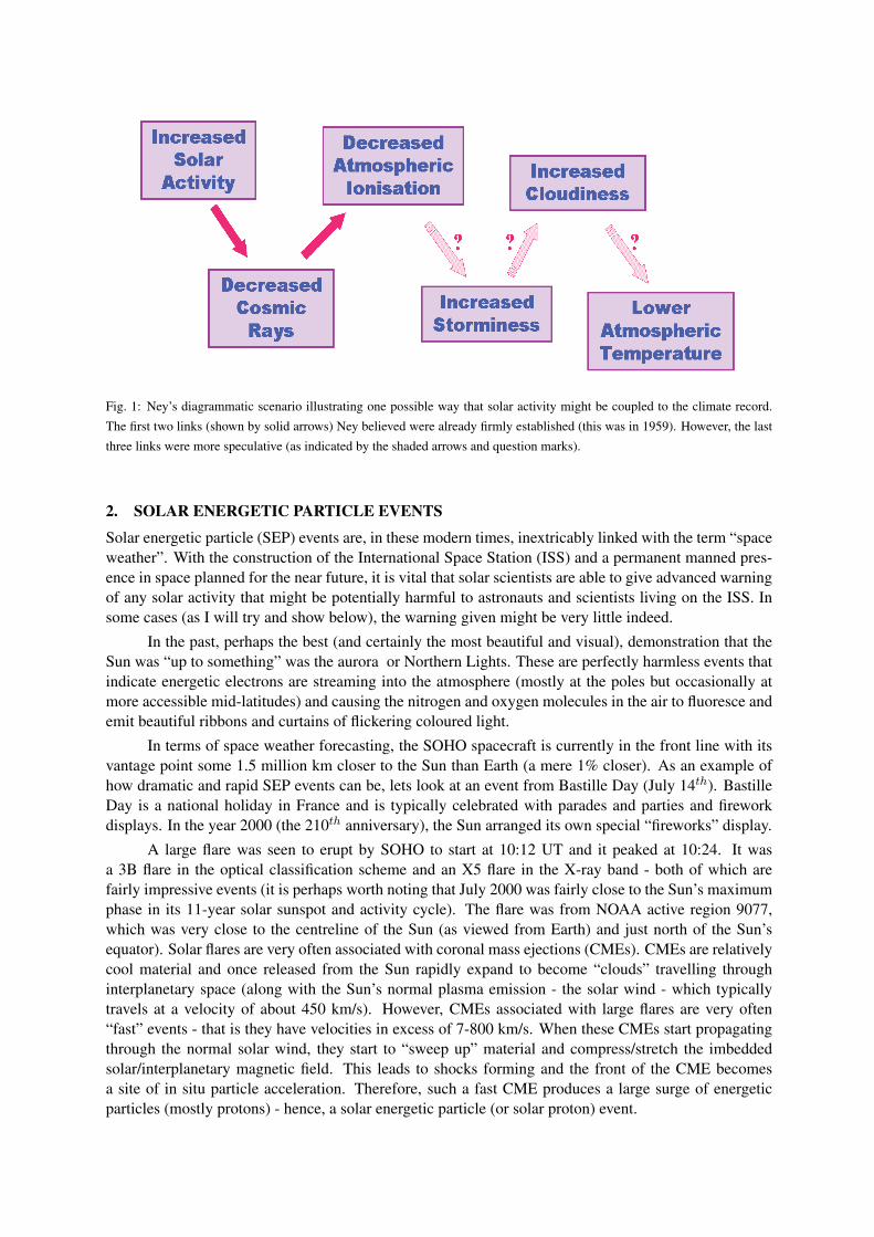
Fig. 1: Ney’s diagrammatic scenario illustrating one possible way that solar activity might be coupled to the climate record.

The first two links (shown by solid arrows) Ney believed were already firmly established (this was in 1959). However, the last

three links were more speculative (as indicated by the shaded arrows and question marks).

2. SOLAR ENERGETIC PARTICLE EVENTS

Solar energetic particle (SEP) events are, in these modern times, inextricably linked with the term “spaceweather”. With the construction of the International Space Station (ISS) and a permanent manned pres-ence in space planned for the near future, it is vital that solar scientists are able to give advanced warningof any solar activity that might be potentially harmful to astronauts and scientists living on the ISS. Insome cases (as I will try and show below), the warning given might be very little indeed.

In the past, perhaps the best (and certainly the most beautiful and visual), demonstration that theSun was “up to something” was the aurora or Northern Lights. These are perfectly harmless events thatindicate energetic electrons are streaming into the atmosphere (mostly at the poles but occasionally atmore accessible mid-latitudes) and causing the nitrogen and oxygen molecules in the air to fluoresce andemit beautiful ribbons and curtains of flickering coloured light.

In terms of space weather forecasting, the SOHO spacecraft is currently in the front line with itsvantage point some 1.5 million km closer to the Sun than Earth (a mere 1% closer). As an example ofhow dramatic and rapid SEP events can be, lets look at an event from Bastille Day (July 14th). BastilleDay is a national holiday in France and is typically celebrated with parades and parties and fireworkdisplays. In the year 2000 (the 210th anniversary), the Sun arranged its own special “fireworks” display.

A large flare was seen to erupt by SOHO to start at 10:12 UT and it peaked at 10:24. It wasa 3B flare in the optical classification scheme and an X5 flare in the X-ray band - both of which arefairly impressive events (it is perhaps worth noting that July 2000 was fairly close to the Sun’s maximumphase in its 11-year solar sunspot and activity cycle). The flare was from NOAA active region 9077,which was very close to the centreline of the Sun (as viewed from Earth) and just north of the Sun’sequator). Solar flares are very often associated with coronal mass ejections (CMEs). CMEs are relativelycool material and once released from the Sun rapidly expand to become “clouds” travelling throughinterplanetary space (along with the Sun’s normal plasma emission - the solar wind - which typicallytravels at a velocity of about 450 km/s). However, CMEs associated with large flares are very often“fast” events - that is they have velocities in excess of 7-800 km/s. When these CMEs start propagatingthrough the normal solar wind, they start to “sweep up” material and compress/stretch the imbeddedsolar/interplanetary magnetic field. This leads to shocks forming and the front of the CME becomesa site of in situ particle acceleration. Therefore, such a fast CME produces a large surge of energeticparticles (mostly protons) - hence, a solar energetic particle (or solar proton) event.

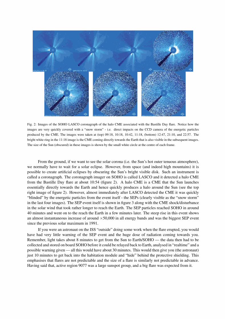
Fig. 2: Images of the SOHO LASCO coronagraph of the halo CME associated with the Bastille Day flare. Notice how the

images are very quickly covered with a “snow storm” - i.e. direct impacts on the CCD camera of the energetic particles

produced by the CME. The images were taken at (top) 09:18, 10:18, 10:42, 11:18, (bottom) 12:47, 21:10, and 22:57. The

bright white ring in the 11:18 image is the CME coming directly towards the Earth that is also visible in the subsequent images.

The size of the Sun (obscured) in these images is shown by the small white circle at the centre of each frame.

From the ground, if we want to see the solar corona (i.e. the Sun’s hot outer tenuous atmosphere),we normally have to wait for a solar eclipse. However, from space (and indeed high mountains) it ispossible to create artificial eclipses by obscuring the Sun’s bright visible disk. Such an instrument iscalled a coronagraph. The coronagraph imager on SOHO is called LASCO and it detected a halo CMEfrom the Bastille Day flare at about 10:54 (figure 2). A halo CME is a CME that the Sun launchesessentially directly towards the Earth and hence quickly produces a halo around the Sun (see the topright image of figure 2). However, almost immediately after LASCO detected the CME it was quickly“blinded” by the energetic particles from the event itself - the SEPs (clearly visible as the “snow storm”in the last four images). The SEP event itself is shown in figure 3 along with the CME shock/disturbancein the solar wind that took rather longer to reach the Earth. The SEP particles reached SOHO in around40 minutes and went on to the reach the Earth in a few minutes later. The steep rise in this event showsan almost instantaneous increase of around ×50,000 in all energy bands and was the biggest SEP eventsince the previous solar maximum in 1991.

If you were an astronaut on the ISS “outside” doing some work when the flare erupted, you wouldhave had very little warning of the SEP event and the huge dose of radiation coming towards you.Remember, light takes about 8 minutes to get from the Sun to Earth/SOHO — the data then had to becollected and stored on board SOHO before it could be relayed back to Earth, analysed in “realtime” and apossible warning given — all this would have about 30 minutes. This would then give you (the astronaut)just 10 minutes to get back into the habitation module and “hide” behind the protective shielding. Thisemphasises that flares are not predictable and the size of a flare is similarly not predictable in advance.Having said that, active region 9077 was a large sunspot group, and a big flare was expected from it.

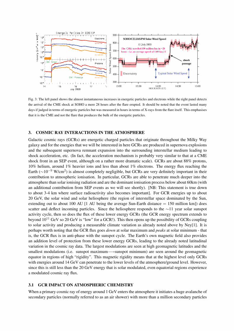
Fig. 3: The left panel shows the almost instantaneous increases in energetic particles and electrons while the right panel detects

the arrival of the CME shock at SOHO a mere 28 hours after the flare erupted. It should be noted that the event lasted many

days if judged in terms of energetic particles but was measured in hours in terms of X-rays from the flare itself. This emphasises

that it is the CME and not the flare that produces the bulk of the energetic particles.

3. COSMIC RAY INTERACTIONS IN THE ATMOSPHERE

Galactic cosmic rays (GCRs) are energetic charged particles that originate throughout the Milky Waygalaxy and for the energies that we will be interested in here GCRs are produced in supernova explosionsand the subsequent supernova remnant expansion into the surrounding interstellar medium leading toshock acceleration, etc. (In fact, the acceleration mechanism is probably very similar to that at a CMEshock front in an SEP event, although on a rather more dramatic scale). GCRs are about 88% protons,10% helium, around 1% heavier ions and less than about 1% electrons. The energy flux reaching theEarth (∼10−9 W/cm2) is almost completely negligible, but GCRs are very definitely important in theircontribution to atmospheric ionisation. In particular, GCRs are able to penetrate much deeper into theatmosphere than solar ionising radiation and are the dominant ionisation process below about 60km (withan additional contribution from SEP events as we will see shortly). [NB: This statement is true downto about 3-4 km where surface radioactivity also becomes important]. For GCR energies up to about20 GeV, the solar wind and solar heliosphere (the region of interstellar space dominated by the Sun,extending out to about 100 AU [1 AU being the average Sun-Earth distance = 150 million km]) doesscatter and deflect incoming particles. Since the heliosphere responds to the ∼11 year solar sunspotactivity cycle, then so does the flux of these lower energy GCRs (the GCR energy spectrum extends tobeyond 1011 GeV so 20 GeV is “low” for a GCR!). This then opens up the possibility of GCRs couplingto solar activity and producing a measurable climate variation as already noted above by Ney[1]. It isperhaps worth noting that the GCR flux goes down at solar maximum and peaks at solar minimum - thatis, the GCR flux is in anti-phase with the sunspot cycle. The Earth’s own magnetic field also providesan addition level of protection from these lower energy GCRs, leading to the already noted latitudinalvariation in the cosmic ray data. The largest modulations are seen at high geomagnetic latitudes and thesmallest modulations (i.e. sunspot maximum−→sunspot minimum) are seen around the geomagneticequator in regions of high “rigidity”. This magnetic rigidity means that at the highest level only GCRswith energies around 14 GeV can penetrate to the lower levels of the atmosphere/ground level. However,since this is still less than the 20 GeV energy that is solar modulated, even equatorial regions experiencea modulated cosmic ray flux.

3.1 GCR IMPACT ON ATMOSPHERIC CHEMISTRY

When a primary cosmic ray of energy around 1 GeV enters the atmosphere it initiates a huge avalanche ofsecondary particles (normally referred to as an air shower) with more than a million secondary particles

produced. This flux of secondary particles increases as we traverse down through the atmosphere untilwe reach around 15–25 km (depending on magnetic rigidity and solar cycle phase) below which the fluxdecreases again. (The ionisation maximum height is more correctly a measure of the total atmosphericcolumn density traversed by the secondaries, which is equivalent to saying the atmospheric pressure).In this paper it is not the ionisation itself that I wish to consider, but the atmospheric chemistry thatmight result from cosmic rays hitting the atmosphere. Given that the atmosphere is essentially made ofnitrogen (N2), oxygen (O2) and a trace of water vapour (H2O), it shouldn’t be to surprising that the majorchemical species generated by GCRs are oxides of nitrogen and hydrogen — so called NOx and HOx.[NOx — N, NO, NO2; HOx — H, OH, HO2]. There is also a secondary effect on ozone which will bebriefly discussed.

Warneck[2] was the first to note that GCRs would be a significant source of NOx (and particularlyNO). (This was around the time that ozone destruction was beginning to be studied and aircraft emissionsand other manmade contributions had already been considered as a possible culprit). However, it wasNicolet[3] who first calculated production rates of nitric oxide (NO) by GCRs and also the variationcaused by the solar modulation. These calculations showed a large production and modulation effectat high geomagnetic latitude (above 50 latitude) at an altitude of 20 km. Some of the more importantreactions are shown below.

N2 → N + N+ O2 → O + O+ (dissociative ionisation) (1)

N+ + O2 → O+2 + N N+ + O2 → O + NO+ N2 + O+

2 → NO + NO+ (2)

NO + O3 → O2 + NO2 NO2 + O3 → O2 + NO3 OH + NO2 + M → HNO3 + M (3)

OH + O → O2 + H H + O3 → OH + O2 OH + O3 → H2O + O2 (4)

As can be seen in (3) and (4) HOx and NOx are implicated in ozone destruction. However, it isnot just galactic cosmic rays that promote these atmospheric reactions — solar energetic particles canalso be important. The only key difference is that SEPs produce their effects in the middle atmospherewhile GCRs produce effects, in particular, in the lower stratosphere and upper troposphere. At least nineseparate SEP events have been observed to produce ozone depletions in the past three solar cycles, andone of the most dramatic events was the August 1972 SEP. These ozone depletions are believed to be pri-marily due to the newly created HOx species, although the role of NOx cannot be underestimated. Thereis another difference between GCR and SEPs — SEPs occur most frequently around solar maximum, inparticular on the rise just prior to maximum and on the fall a year or two after maximum, while GCRspeak around solar minimum.

Jackman et al. [4] looked in detail at the various sources of nitric oxide and where in the atmo-sphere each process is effective (figure 4). They showed that stratospheric NO is mainly produced fromthe dissociation of nitrous oxide (N2O) - which is a by-product of the biological nitrogen cycle. Thisprovides a large and relatively constant background source. However, GCRs and SEPs provide a signif-icant and variable component of NO in the middle atmosphere. In fact, at geomagnetic latitudes greaterthan 50, the GCR contribution shows a solar cycle modulation of some 50% and is also responsible forabout 50% of the total NO production in the stratosphere and mesosphere. Jackman et al. [4] also madedetailed calculations for some SEP events. In particular, they showed that the large event in August, 1972(around three years after solar maximum) produced effects that extended down to 10 km. It also took theatmosphere 1 year to return to pre-event levels.

4. LIGHTNING AS A SOURCE OF NOx

As can be seen in figure 4, lightning is listed as a major contributor to NO production in the atmosphere.The role of lightning was studied in more detail by Legrand et al. [5]. Lightning generates NO by thethermal decomposition of nitrogen and oxygen, and this is likely to be especially important in the Tropicsand in the lower regions of the atmosphere (as can be seen in figure 4, where lightning is the only source

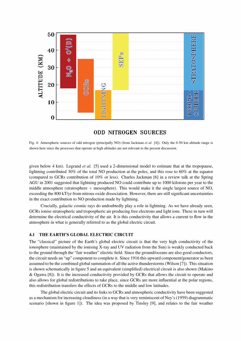
Fig. 4: Atmospheric sources of odd nitrogen (principally NO) (from Jackman et al. [4]). Only the 0-50 km altitude range is

shown here since the processes that operate at high altitudes are not relevant to the present discussion.

given below 4 km). Legrand et al. [5] used a 2-dimensional model to estimate that at the tropopause,lightning contributed 30% of the total NO production at the poles, and this rose to 60% at the equator(compared to GCRs contribution of 10% or less). Charles Jackman [6] in a review talk at the SpringAGU in 2001 suggested that lightning produced NO could contribute up to 1000 kilotons per year to themiddle atmosphere (stratosphere + mesosphere). This would make it the single largest source of NO,exceeding the 800 kT/yr from nitrous oxide dissociation. However, there are still significant uncertaintiesin the exact contribution to NO production made by lightning.

Crucially, galactic cosmic rays do undoubtedly play a role in lightning. As we have already seen,GCRs ionise stratospheric and tropospheric air producing free electrons and light ions. These in turn willdetermine the electrical conductivity of the air. It is this conductivity that allows a current to flow in theatmosphere in what is generally referred to as the global electric circuit.

4.1 THE EARTH’S GLOBAL ELECTRIC CIRCUIT

The “classical” picture of the Earth’s global electric circuit is that the very high conductivity of theionosphere (maintained by the ionising X-ray and UV radiation from the Sun) is weakly conducted backto the ground through the “fair weather” electric field. Since the ground/oceans are also good conductors,the circuit needs an “up” component to complete it. Since 1916 this upward component/generator as beenassumed to be the combined global summation of all the active thunderstorms (Wilson [7]). This situationis shown schematically in figure 5 and an equivalent (simplified) electrical circuit is also shown (Makino& Ogawa [8]). It is the increased conductivity provided by GCRs that allows the circuit to operate andalso allows for global redistributions to take place, since GCRs are more influential at the polar regions,this redistribution transfers the effects of GCRs to the middle and low latitudes.

The global electric circuit and its links to GCRs and atmospheric conductivity have been suggestedas a mechanism for increasing cloudiness (in a way that is very reminiscent of Ney’s (1959) diagrammaticscenario [shown in figure 1]). The idea was proposed by Tinsley [9], and relates to the fair weather

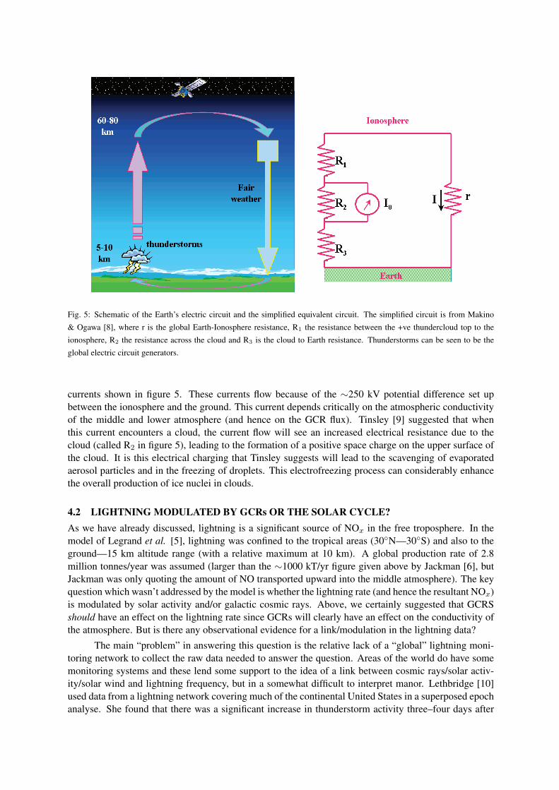
Fig. 5: Schematic of the Earth’s electric circuit and the simplified equivalent circuit. The simplified circuit is from Makino

& Ogawa [8], where r is the global Earth-Ionosphere resistance, R1 the resistance between the +ve thundercloud top to the

ionosphere, R2 the resistance across the cloud and R3 is the cloud to Earth resistance. Thunderstorms can be seen to be the

global electric circuit generators.

currents shown in figure 5. These currents flow because of the ∼250 kV potential difference set upbetween the ionosphere and the ground. This current depends critically on the atmospheric conductivityof the middle and lower atmosphere (and hence on the GCR flux). Tinsley [9] suggested that whenthis current encounters a cloud, the current flow will see an increased electrical resistance due to thecloud (called R2 in figure 5), leading to the formation of a positive space charge on the upper surface ofthe cloud. It is this electrical charging that Tinsley suggests will lead to the scavenging of evaporatedaerosol particles and in the freezing of droplets. This electrofreezing process can considerably enhancethe overall production of ice nuclei in clouds.

4.2 LIGHTNING MODULATED BY GCRs OR THE SOLAR CYCLE?

As we have already discussed, lightning is a significant source of NOx in the free troposphere. In themodel of Legrand et al. [5], lightning was confined to the tropical areas (30N—30S) and also to theground—15 km altitude range (with a relative maximum at 10 km). A global production rate of 2.8million tonnes/year was assumed (larger than the ∼1000 kT/yr figure given above by Jackman [6], butJackman was only quoting the amount of NO transported upward into the middle atmosphere). The keyquestion which wasn’t addressed by the model is whether the lightning rate (and hence the resultant NOx)is modulated by solar activity and/or galactic cosmic rays. Above, we certainly suggested that GCRSshould have an effect on the lightning rate since GCRs will clearly have an effect on the conductivity ofthe atmosphere. But is there any observational evidence for a link/modulation in the lightning data?

The main “problem” in answering this question is the relative lack of a “global” lightning moni-toring network to collect the raw data needed to answer the question. Areas of the world do have somemonitoring systems and these lend some support to the idea of a link between cosmic rays/solar activ-ity/solar wind and lightning frequency, but in a somewhat difficult to interpret manor. Lethbridge [10]used data from a lightning network covering much of the continental United States in a superposed epochanalyse. She found that there was a significant increase in thunderstorm activity three–four days after

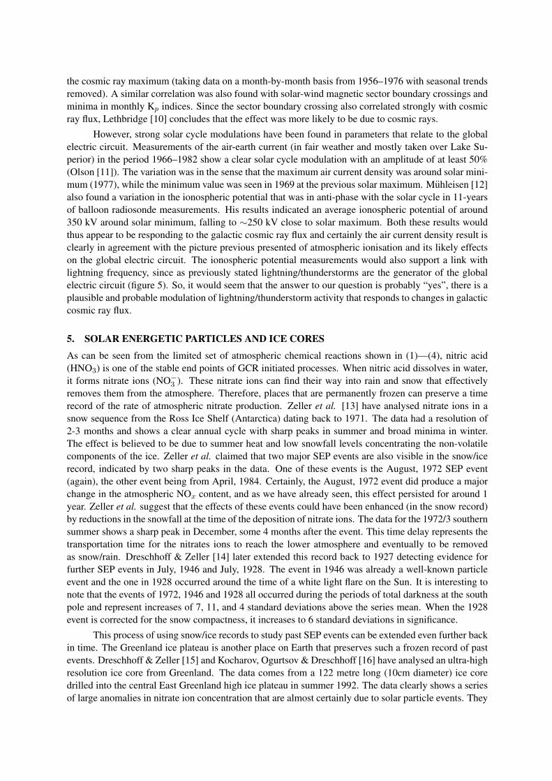
the cosmic ray maximum (taking data on a month-by-month basis from 1956–1976 with seasonal trendsremoved). A similar correlation was also found with solar-wind magnetic sector boundary crossings andminima in monthly Kp indices. Since the sector boundary crossing also correlated strongly with cosmicray flux, Lethbridge [10] concludes that the effect was more likely to be due to cosmic rays.

However, strong solar cycle modulations have been found in parameters that relate to the globalelectric circuit. Measurements of the air-earth current (in fair weather and mostly taken over Lake Su-perior) in the period 1966–1982 show a clear solar cycle modulation with an amplitude of at least 50%(Olson [11]). The variation was in the sense that the maximum air current density was around solar mini-mum (1977), while the minimum value was seen in 1969 at the previous solar maximum. Muhleisen [12]also found a variation in the ionospheric potential that was in anti-phase with the solar cycle in 11-yearsof balloon radiosonde measurements. His results indicated an average ionospheric potential of around350 kV around solar minimum, falling to ∼250 kV close to solar maximum. Both these results wouldthus appear to be responding to the galactic cosmic ray flux and certainly the air current density result isclearly in agreement with the picture previous presented of atmospheric ionisation and its likely effectson the global electric circuit. The ionospheric potential measurements would also support a link withlightning frequency, since as previously stated lightning/thunderstorms are the generator of the globalelectric circuit (figure 5). So, it would seem that the answer to our question is probably “yes”, there is aplausible and probable modulation of lightning/thunderstorm activity that responds to changes in galacticcosmic ray flux.

5. SOLAR ENERGETIC PARTICLES AND ICE CORES

As can be seen from the limited set of atmospheric chemical reactions shown in (1)—(4), nitric acid(HNO3) is one of the stable end points of GCR initiated processes. When nitric acid dissolves in water,it forms nitrate ions (NO−

3 ). These nitrate ions can find their way into rain and snow that effectivelyremoves them from the atmosphere. Therefore, places that are permanently frozen can preserve a timerecord of the rate of atmospheric nitrate production. Zeller et al. [13] have analysed nitrate ions in asnow sequence from the Ross Ice Shelf (Antarctica) dating back to 1971. The data had a resolution of2-3 months and shows a clear annual cycle with sharp peaks in summer and broad minima in winter.The effect is believed to be due to summer heat and low snowfall levels concentrating the non-volatilecomponents of the ice. Zeller et al. claimed that two major SEP events are also visible in the snow/icerecord, indicated by two sharp peaks in the data. One of these events is the August, 1972 SEP event(again), the other event being from April, 1984. Certainly, the August, 1972 event did produce a majorchange in the atmospheric NOx content, and as we have already seen, this effect persisted for around 1year. Zeller et al. suggest that the effects of these events could have been enhanced (in the snow record)by reductions in the snowfall at the time of the deposition of nitrate ions. The data for the 1972/3 southernsummer shows a sharp peak in December, some 4 months after the event. This time delay represents thetransportation time for the nitrates ions to reach the lower atmosphere and eventually to be removedas snow/rain. Dreschhoff & Zeller [14] later extended this record back to 1927 detecting evidence forfurther SEP events in July, 1946 and July, 1928. The event in 1946 was already a well-known particleevent and the one in 1928 occurred around the time of a white light flare on the Sun. It is interesting tonote that the events of 1972, 1946 and 1928 all occurred during the periods of total darkness at the southpole and represent increases of 7, 11, and 4 standard deviations above the series mean. When the 1928event is corrected for the snow compactness, it increases to 6 standard deviations in significance.

This process of using snow/ice records to study past SEP events can be extended even further backin time. The Greenland ice plateau is another place on Earth that preserves such a frozen record of pastevents. Dreschhoff & Zeller [15] and Kocharov, Ogurtsov & Dreschhoff [16] have analysed an ultra-highresolution ice core from Greenland. The data comes from a 122 metre long (10cm diameter) ice coredrilled into the central East Greenland high ice plateau in summer 1992. The data clearly shows a seriesof large anomalies in nitrate ion concentration that are almost certainly due to solar particle events. They

also measured the conductivity of the ice and this data shows volcanic activity that can be used to “date”the core. For events like Krakatau or Tambora, which are in the southern hemisphere, it is necessary toallow around 1 year for ion transportation to the northern polar regions.

After removing the seasonal background from the nitrate data, it is possible to analyse the longer-term trends in the time series. By smoothing the data with a moving average with a length of about8 years, several features of the series become apparent. There is a small dip in the early 1800s and asecond longer dip from ∼1650–1700. These features correspond (in time at least), to the Dalton andMaunder Minima periods (respectively). These are two intervals when solar activity was at a reducedlevel. Indeed, during the Maunder Minimum, sunspots almost completely disappeared from the Sun’ssurface and several solar cycles had only one or two spots in total. When directly compared to the sunspotdata, the nitrate ion data does not correlate all that well. The lack of quantitative agreement between thetwo data sets reflects the fact that sunspots are not a good measure of solar flares and solar energeticparticle events or the solar wind — which are the two dominant processes that drive nitrate generation(via SEPs and GCRs, respectively).

However, when the data is examined at higher time resolution (i.e. without the smoothing), thensome general agreement between the two sets can be found. Two peaks in particular occurred in 1851and 1849. These could be connected to unusual white light flares seen in Feb., 1851 and Jan., 1849 —1849 is close to sunspot maximum and 1851 is on the declining phase of the solar cycle. This is quitetypical, the largest SEP events generally occur on the rising and declining parts of sunspot cycles - ratherthan at the peaks of the cycles. When the full data series is analysed for periodicities it is found that a∼5 year period is detectable in the data from 1760—1900. This period is almost exactly half the sunspotcycle and is very compelling evidence for an SEP signature to be present in the data (i.e. the data islikely detecting the rising and falling parts of each ∼11 year cycle). This conclusion was tested by takingthe sunspot data and frequency doubling it (by multiplying the data by its Hilbert transform). This newsunspot series then showed a period at ∼5.3 years, exactly in agreement with the nitrate ion data.

6. CONCLUSIONS

Galactic Cosmic Rays deposit their energy in the low stratosphere and produce NO at ratios dependingon the phase of the solar cycle — this accounts for approximately half the NO at high latitudes and witha large ∼ 11-year modulation. Solar Energetic Particles Events occur sporadically but are more frequentaround solar maximum. They interact with the atmosphere in the 30-60 km range but occasionallyreach down below 20 km. However, they are useful for studying the effects of energetic particles onatmospheric chemistry because they have essentially instantaneous rise times with very large proton fluxincreases. Lightning is also a potentially important source of NO and is also possibly correlated withGCRs. Ice core data shows that SEP generated nitrates can reach the ground/low atmosphere in largequantities.

So, some 40+ years after Ney’s original paper [1], what progress (if any?) have we made in in-vestigating the role that cosmic rays (or the resultant atmospheric ionisation) might be having on climateand/or meteorology? Certainly, the correlation reported by Svensmark & Friis-Christensen [17] betweenglobal cloud cover and galactic cosmic rays gave renewed vigour to the solar-activity–climate debate. Ifthe link is correct it actually goes in the opposite sense to Ney’s original suggestion (figure 1). The exactdetails of the observational link between cloud cover and cosmic rays was refined when better clouddata became available (Marsh & Svensmark [18]). This showed a very striking correlation between lowclouds and cosmic rays and in particular for low cloud top temperature which on the global correlationmaps shows a clear and strong positive correlation for clouds in the Tropics. This latter links (i.e. lowclouds and Tropics) then suggests a possible link with lightning which was shown above to also havean association with the Tropics and to be the only NOx process to operate below 5 km. Therefore, Iwould like to conclude this overview with my own updated “Ney Diagrammatic Scenario” (figure 6).Once again, like Ney [1], I would like to stress that this is only my suggested series of links and more

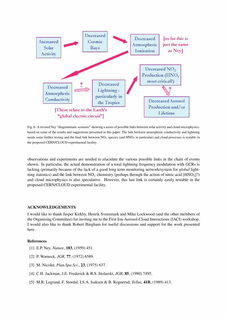
Fig. 6: A revised Ney “diagrammatic scenario” showing a series of possible links between solar activity and cloud microphysics,

based on some of the results and suggestions presented in this paper. The link between atmospheric conductivity and lightning

needs some further testing and the final link between NOx species (and HNO3 in particular) and cloud processes is testable in

the proposed CERN/CLOUD experimental facility.

observations and experiments are needed to elucidate the various possible links in the chain of eventsshown. In particular, the actual demonstration of a total lightning frequency modulation with GCRs islacking (primarily because of the lack of a good long term monitoring network/system for global light-ning statistics) and the link between NOx chemistry (perhaps through the action of nitric acid [HNO3]?)and cloud microphysics is also speculative. However, this last link is certainly easily testable in theproposed CERN/CLOUD experimental facility.

ACKNOWLEDGEMENTS

I would like to thank Jasper Kirkby, Henrik Svensmark and Mike Lockwood (and the other members ofthe Organising Committee) for inviting me to the First Ion-Aerosol-Cloud Interactions (IACI) workshop.I would also like to thank Robert Bingham for useful discussions and support for the work presentedhere.

References

[1] E.P. Ney, Nature, 183, (1959) 451.

[2] P. Warneck, JGR, 77, (1972) 6589.

[3] M. Nicolet, Plan.Spa.Sci., 23, (1975) 637.

[4] C.H. Jackman, J.E. Frederick & R.S. Stolarski, JGR, 85, (1980) 7495.

[5] M.R. Legrand, F. Stordal, I.S.A. Isaksen & B. Rognerud, Tellus, 41B, (1989) 413.

[6] C. Jackman & S.R. Kawa, AGUSM, A62A–01 (2001) [invited review talk].

[7] C.T.R. Wilson, Proc. Roy. Soc. A, 92, (1916) 555.

[8] M. Makino & T. Ogawa, JATP, 46 (5), (1984) 431.

[9] B.A. Tinsley, J.Geomag.Geoelec., 48 (1), (1996) 165.

[10] M. Lethbridge, GRL, 8, (1981) 521.

[11] D.E. Olson, in Weather and Climate Responses to Solar Variations, ed. B.M. McCormac (ColoradoAssociated University Press, Boulder), (1983) 483.

[12] R. Muhleisen, in Electrical Processes & Atmospheres, eds. H. Dolezalek & R. Reiter (SteinkopffVerlag, Darmstadt), (1977) 467.

[13] E.J. Zeller, G.A.M. Dreschhoff & C.M. Laird, GRL, 13 (12), (1986) 1264.

[14] G.A.M. Dreschhoff & E.J. Zeller, Sol.Phys., 127, (1990) 333.

[15] G.A.M. Dreschhoff & E.J. Zeller, Sol.Phys., 177, (1998) 365.

[16] G.E. Kocharov, M.G. Ogurtsov & G.A.M. Dreschhoff, Sol.Phys, 188, (1999) 187.

[17] H. Svensmark & E. Friis-Christensen, JATP, 59, (1997) 1225.

[18] N. Marsh & H. Svensmark, Spa.Sci.Rev., 94, (2000) 215.

EXPERIMENTS ON NUCLEATION PROCESSES IN AEROSOLS

P. E. WagnerInstitut für Experimentalphysik der Universität Wien, Vienna, Austria

AbstractVarious dynamical processes observed in the atmosphere are related to phasetransitions from the gas phase. In this presentation selected experimentalstudies on nucleation and condensation processes are reviewed and theirrelevance to atmospheric aerosols is discussed. Open questions remainparticularly for phase transitions in binary and multicomponent systems andin the field of ion-induced nucleation. Furthermore, the influence ofmiscibility and solubility of the compounds considered has not yet beenclarified sufficiently.

1. INTRODUCTION

Nucleation processes in the gas phase are of considerable importance in connection with formationand dynamical behaviour of atmospheric aerosols. While homogeneous nucleation in one-componentvapor systems will generally not occur in the atmosphere, binary or multicomponent homogeneousnucleation are quite relevant to atmospheric aerosol formation [1-4]. Aerosol and cloud dropformation in the atmosphere are frequently connected with heterogeneous nucleation on soluble orinsoluble particles and with ion-induced nucleation.

The accuracy of nucleation experiments depends on the preparation of mixtures of inert gaseswith condensable vapors at well-defined thermodynamic conditions. This can be achieved byadiabatic expansion of initially saturated vapor-gas mixtures. In the present contribution expansionchamber studies on homogeneous and on heterogeneous nucleation will be discussed. The nucleatedparticles can be observed by the Constant-Angle Mie Scattering (CAMS) method [5]. The CAMS-detector allows non-invasive quantitative monitoring of number concentration and diameter of thecondensing particles.

2. METHODS OF OBSERVATION

A crucial condition for well-defined experimental studies of nucleation and condensation processes isthe preparation of mixtures of an inert gas with condensable vapors at accurately determinedsupersaturations (vapor phase activities, partial vapor pressures) and temperatures. The followingtechniques have been successfully applied for this purpose: Nonisothermal vapor diffusion in static [6,7] or steady state flow [8, 9] systems, adiabatic expansion [10, 11] and turbulent mixing [12] . Asdirect measurement of the temperature in supersaturated vapors is complicated, usually temperatureand supersaturations need to be calculated.

Nucleation processes can generally not be detected directly. Only the particles growingsubsequent to the formation of the critical clusters, are observed. The concentrations of condensingdroplets can be measured by single particle counting. The Constant-Angle Mie Scattering (CAMS)method [5] allows simultaneous and independent determination of concentration and size of growingdroplets during condensation.

3. THE EXPANSION CHAMBER METHOD

Supersaturated vapor - carrier gas mixtures can be prepared in expansion chambers (see, e.g., [13]).To this end a saturated or nearly saturated mixture of the gaseous components considered isadiabatically expanded in an expansion chamber. Corresponding to the adiabatic temperature dropoccurring in the chamber, supersaturated vapors with well-defined vapor saturation ratios areobtained. An accurate straightforward determination of temperature drop and vapor saturation ratio ispossible, if the carrier gas - vapor mixture is nearly an ideal gas and if no significant vaporcondensation occurs already during the expansion (dry-adiabatic expansion). Approximately dry-adiabatic expansions can only be achieved, if the time interval, during which the expansion occurs, issmall compared to the typical times required for condensational growth at the conditions considered.

For expansion chamber studies of homogeneous nucleation a further condition is essential. Ashomogeneous nucleation and droplet growth generally occur simultaneously, the depletion of vaporcaused by the condensational drop growth process will lead to a reduction of vapor supersaturationthereby quenching the homogeneous nucleation process. In order to obtain quantitative informationon homogeneous nucleation rates, it is therefore important to decouple nucleation and growth. Thiscan be achieved by means of the nucleation pulse technique [10, 11].

The droplets growing in the expansion chamber can be quantitatively observed by means of theCAMS detection method [5]. To this end the droplets are illuminated by a laser beam. The light fluxtransmitted through the expansion chamber as well as the light flux scattered at a selectable constantscattering angle are monitored simultaneously. The scattered light flux shows series of extrema ingood agreement with the prediction by Mie theory (see [5]). After establishing a uniquecorrespondence between experimental and theoretical light scattering extrema, size and numberconcentration of the growing droplets can be determined by quantitative comparison of experimentaland theoretical light fluxes. Light attenuation in the expansion chamber can be accounted for bynormalizing the scattered relative to the transmitted light fluxes.

The following features of the expansion chamber method are notable:

(1) Temperature and vapor saturation ratios (vapor phase activities) in expansion chambers can bedetermined accurately by means of a straightforward procedure,

(2) Vapor supersaturation can be achieved during a comparatively short time interval,

(3) Temperature and vapor saturation ratios obtained in the measuring volume are uniform,

(4) Number concentration and size of growing droplets can be measured at various times during thegrowth process by means of a non-invasive and absolute method (CAMS detection).

4. EXPERIMENTAL RESULTS

Homogeneous nucleation in unary vapors has been studied for various compounds generally showingfair agreement with theory. Particularly the experimental slopes of the nucleation rate vs.supersaturation curves agree well with theory. However, experiments for binary and ternary vapormixtures [14-19] frequently result in substantial deviations from classical nucleation theory,particularly for non-ideal mixtures. Homogeneous nucleation of partially immiscible liquids shows asomewhat complex behaviour.

The few so far available quantitative experiments on heterogeneous nucleation have beenrestricted to unary systems. Only recently we have reported first experimental studies on binary

heterogeneous nucleation [20]. These studies show that the macroscopic contact angle is hardlyapplicable for heterogeneous nucleation on nano-particles.

5. CONCLUSIONS

Expansion chamber experiments are suitable for time-resolved measurements of nucleation andcondensation processes. For the purpose of modeling of atmospheric conditions expansion chambershave the important feature that the thermodynamical conditions in the measuring volume are uniformand can be accurately determined. Experiments on homogeneous nucleation typically show fairagreement with the classical nucleation theory for unary systems, whereas severe discrepancies forsome multicomponent systems have been encountered. The interpretation of heterogeneousnucleation measurements depends on the choice of the contact angle.

ACKNOWLEDGMENTS

This work has been supported by the Fonds zur Förderung der Wissenschaftlichen Forschung, Proj.Nr. P 9421 and by the Hochschuljubiläumsstiftung der Stadt Wien.

REFERENCES

[1] Raes, F., and Van Dingenen, R., J. Geophys. Res. 97, 12901 (1992).

[2] Arstila, H., Korhonen, P., Kulmala, M., J. Aerosol Sci. 30, 131 (1999).

[3] Mäkelä, J. M., Aalto, P., Jokinen, V., Pohja, T., Nissinen, A., Palmroth, S., Markkanen, T.,Seitsonen, K., Lihavainen, H., and Kulmala, M., Geophys. Res. Lett. 24, 1219 (1997).

[4] Kulmala, M., Pirjola, L., and Mäkelä, J. M., Nature 404, 67 (2000).

[5] Wagner, P. E., J. Colloid Interface Sci. 105, 456 (1985).

[6] Katz, J. L., and Ostermier, M., J. Chem. Phys. 47, 478 (1967).

[7] Hung, C., Krasnopoler, M., J., and Katz, J. L., J. Chem. Phys. 90, 1856 (1989).

[8] Anisimov, M. P., and Cherevko, A. G., J. Aerosol Sci. 16, 97 (1985).

[9] Wilck, M., Hämeri, K., Stratmann, F., and Kulmala, M., J. Aerosol Sci. 29, 899 (1998).

[10] Schmitt, J. L., Adams, G. W., and Zalabsky, R. A., J. Chem. Phys. 77, 2089 (1982).

[11] Wagner, P. E., and Strey, R., J. Chem. Phys. 80, 5266 (1984).

[12] Wyslouzil, B. E., Seinfeld, J. H., and Flagan, R., C., J. Chem. Phys. 94, 6842 (1991).

[13] Wagner. P. E., in Aerosol Microphysics II (W. H. Marlow, Ed.) p.129. Springer, Berlin, 1982.

[14] Wilemski, G., J. Phys. Chem. 91, 2492 (1987).

[15] Schmitt, J. L., Whitten, J., Adams, G. W., and Zalabsky, R. A., J. Chem. Phys. 92, 3693 (1990).

[16] Wyslouzil, B. E., Seinfeld, J. H., Flagan, R. C., and Okuyama, K., J. Chem. Phys. 94, 6842(1991).

[17] Strey, R., Viisanen, Y., and Wagner, P. E., J. Chem. Phys. 103, 4333 (1995).

[18] Viisanen, Y., Wagner, P. E., and Strey, R., J. Chem. Phys. 108, 4257 (1998).

[19] Viisanen, Y., and Strey, R., J. Chem. Phys. 105, 8293 (1996).

[20] Petersen, D., Ortner, R., Vrtala, A., Laaksonen, A., Kulmala, M., and Wagner, P. E., J. AerosolSci. 30, S35 (1999).

COMMENTS ON THE OPERATION OF A WILSON EXPANSIONCLOUD CHAMBER

John L. SchmittPhysics Department and Cloud and Aerosol Sciences Laboratory, University of Missouri-Rolla,Rolla, MO, 65401 USA

AbstractComments are made concerning the practical operation of a Wilsonexpansion cloud chamber for experimental research in heterogeneousand homogenous nucleation. Topics covered are the general operationof the chamber, the detection of cloud droplets, the cleaning of thechamber and the interpretation of nucleation data. The commentsinclude successful and unsuccessful experimental techniques.

1. INTRODUCTION

The main experimental apparatus proposed for the CLOUDS investigation is a Wilson expansioncloud chamber. The following comments are intended to provide guidance in the operation ofthat chamber by examining what has been done while operating an expansion chamber at theCloud and Aerosol Sciences Laboratory at the University of Missouri-Rolla. The comments arebased on about 25 years experience by the author operating a chamber (designed forhomogeneous nucleation experiments). This article is intended to supplement Refs. [1, 2] by theauthor and other publications, e. g. Refs. [3, 4]. Reference [1] is a description of the cloudchamber as constructed and used by the author. While the basic features of that chamber have notchanged, this article does address some of the evolutionary changes that have taken place since itwas constructed. Reference [2] describes a Wilson cloud chamber, the UMR absolute Aitkennucleus counter, that was specifically built to detect particles that nucleate from near 100%Relative Humidity to beyond the ion limit. That chamber no longer exists. Reference [3] is areview paper that addresses the “Wilson Cloud Chamber and Its Applications in Physics” circa1946 and still contains much valuable information. Reference [4] is a book by J. G. Wilson (notC. T. R. Wilson) which reviews the Wilson cloud chamber circa 1951. The following commentsinclude improvements, attempted improvements, suggestions, speculations and failures. Again thisarticle primarily addresses experiments with the author’s apparatus, and therefore the referencesand anecdotal evidence are greatly skewed towards work done at high supersaturation with thatdevice.

2. GENERAL OPERATION

2.1 Chamber principles

The physical operating principle of the expansion chamber is that if a gas, containing acondensable vapor at equilibrium, is “suddenly” expanded, the temperature of the gas willadiabatically decrease. In the following, the background carrier gas in the chamber will bereferred to as the gas and the condensable vapor as the vapor. At the lower, expanded,temperature the equilibrium vapor pressure of the vapor is much lower and since the vapor has nothad time to diffuse, it is present at a higher concentration than equilibrium, i. e. supersaturated.Thus the expansion chamber is a device that produces a supersaturation upon demand(expansion). Formally, supersaturation ratio is the ratio of the actual vapor pressure in thechamber divided by its equilibrium vapor pressure at the given temperature but will be referred toin the following as only supersaturation. The length of time for which one knows, to the requiredaccuracy, the physical conditions, temperature and vapor content, in the central volume of the

chamber during and after the expansion, is controlled primarily by the transit (time) of heat andvapor from the walls.

The material or substance in the liquid pool in the case of homogenous nucleation isdetermined by the experiment. For atmospheric simulation water would be the material of choice.For ion nucleation, the classical mixture, used to detect ion tracks for nuclear physics, is about 1part water and 2 parts ethyl alcohol, Ref. [3] pg. 237, which produces the smallest expansion ratiofor the mixture to nucleate on ions.

2.2 Physical parameters in the chamber

Initial conditions in the chamber are temperature, pressure and vapor content of the gas.Temperature and pressure are measured by sensors and the vapor content of the carrier gas isknown from the equilibrium vapor pressure of the liquid pool or by flushing with gas of knowntemperature and vapor content Ref. [5]. The conditions during and after the expansion arecalculated from initial temperature and pressure, the expanded pressure and the thermodynamicproperties of the gas and the vapor. Pressure equilibrates at the speed of sound, however note thatthe speed of sound is not constant, thus pressure can be a valid parameter to describe theconditions in the experimental volume of the chamber. Direct measurement of the temperaturein the experimental volume is very difficult since a sensor larger than molecular size in the centralvolume will probably induce heterogeneous nucleation, along with latent heat release. Laserspectroscopy of a carefully selected molecule has been suggested as method of temperaturemeasurement Ref. [6] but this suggestion has not been implemented. Problems lie in the areas ofisolating and measuring molecules only in the central experimental volume and finding amolecule that not only has the desired temperature range and sufficient sensitivity to measuretemperature to 0.1 C but also will not interact with the desired nucleation. However, such amolecule could be present in large numbers and this application of laser spectroscopy does nothave the same problem as attempting to apply laser spectroscopy to nucleation embryos that arepresent in very low concentrations. A typical temperature calculation ranges from simple, for anadiabatic expansion in a perfect gas with a minor nearly ideal vapor component (the calculationprimarily is the integration of specific heat as a function of temperature), to complex, for a realgas with a significant pressure contribution from real vapor. Argon works well for the gas: it isideal and it does not leak through seals easily. Helium leaks easily, has a high heat conductivityand new gas cylinders of helium often produces alpha particle tracks Ref. [7]. Air is not an idealgas but would be needed for simulating the atmosphere. Additional complexity is added if heatand vapor from the chamber walls reach the experimental volume during the experiment anddroplet growth, with attendant latent heat release and vapor depletion, occurs. In each caseaccurate thermodynamic data for the gas and vapor is essential. If one considers the best case ofan ideal gas and a low vapor pressure vapor, the gas mixture is very close to ideal since thecontribution to the specific heat by the vapor is small. This also means that the thermodynamicdata for the vapor can be uncertain since its contribution is small. In addition, the mixture willproduce a maximum temperature change on expansion.

2.3 Nucleation pulse technique

The nucleation “pulse” technique is often used: the chamber is expanded quickly to maximumexpansion, is then recompressed slightly and held at a supersaturation lower than thesupersaturation at the maximum expansion. Since (homogeneous) nucleation is an exponentialprocess as a function of supersaturation, a slight reduction of supersaturation lowers the nucleationrate by orders of magnitude and thus effectively, when the nucleation rate is integrated over timeto calculate the total number of droplets, “all” nucleation occurs very near the maximumsupersaturation. (In practice one determines the nucleation rate, droplets/cm3 sec, from the dropletcount, droplets/cm3, and the integrated pulse length.) This also limits the nucleation to a knowntime and length of time. The droplets grow to detectable size only after the slight recompression.

This limits the latent heat release and vapor depletion due to growing droplets to the time afternucleation and thus conditions in the experimental volume are well known during nucleation.The nucleation pulse technique avoids the problems of simultaneous nucleation and growth.However, these effects will have to be included in the models if the experiment requires thatnucleation and growth take place simultaneously.

2.4 Supersaturation range and detection of low concentrations

The expansion chamber can produce a wide range of supersaturation. Water supersaturation in therange from 1.00 (100% Relative Humidity) to 1.05, nucleates on and detects (aerosol) particles, i.e. heterogeneous nucleation. Much higher supersaturation, e.g. 3.5 and up, will nucleate on anddetect negative ions and even higher supersaturation will homogeneously nucleate water(examples are for expansions from about 300K, initial chamber temperature). The chamber iscapable of detecting by droplet growth, particles from microns in size (particles at the lower limitfor easy detection by Mie light scattering and which do not fall out rapidly) to molecules. Forexample, if one has an molecule, ion, or particle that will nucleate at a lower supersaturation thanthe homogeneous nucleation of the background vapor, then the chamber is able to nucleate andgrow a droplet on that molecule, ion or particle. For reference, a gas at one atmosphere pressurehas about 1019 atoms or molecules/cm3, and one droplet/cm3 can easily be detected by nucleationin a cloud chamber Ref. [8].

2.5 Low supersaturation expansions

The expansion chamber was chosen as a detector for CLOUDS because it can produce a widerange of supersaturation. It has been traditionally used at high supersaturation in homogeneousnucleation experiments. One technique to produce low supersaturation is to introduceundersaturated vapor and then expand that mixture, Ref. [5]. If, on the other hand, theequilibrium vapor pressure of the liquid pool is used to provide the vapor, a mixture in the poolcan produce (an application of Raoults’ Law; one also must know activity coefficients)undersaturation in the vapor. In the case of water, a mixture of tetraethylene glycol and water willinitially undersaturate the chamber in water and require large (volume ratio) expansions toproduce saturation or supersaturation.Ref. [9].

2.6 CLOUD chamber

The considerable precision with which it is anticipated that the piston of the proposed CERN cloudchamber can be controlled, introduces a capability not found in previous expansion cloudchambers. One now can consider not only experiments where the chamber is expanded once to ahigh or low supersaturation to nucleate on particles or ions, but also experiments where theposition of the piston is accurately controlled with time to attempt to program the Supersaturation(pressure) with time. For example, the chamber is expanded to produce a supersaturation highenough to nucleate on an ion and grow a droplet, the chamber is then compressed to evaporate thedroplet and a second expansion is used to detect any re-evaporation nuclei that remain.Experiments of this type have been performed using the UMR simulation chamber Ref. [10].That chamber has the additional and significant advantage of exact control of the wall temperaturewith time (up to 10 C/minute rate of change with 0.02 C accuracy). One can match walltemperature to the gas temperature during the experiments. Obviously experiments of this type inthe CLOUDS chamber will require good models for the transport of heat and vapor and dropletgrowth. Finally the motion of the piston in the proposed CLOUDS chamber does not dependupon a difference in pressure across it, to drive an expansion. The hydraulic cylinder and valvesystem has considerable force and pulls the piston. Therefore, the CLOUDS chamber can be usedwith very low pressures in the experimental volume (for the simulation of high altitudes).However, one needs to be very careful to model these experiments. For example, accuratecalculations for an adiabatic expansion in a low pressure gas that is mostly water vapor at very low

temperatures (the water vapor may be supercooled) and pressures require accuratethermodynamic data. This may be difficult to find or measure.

3. DETECTION OF DROPLETS

3.1 Droplets vs. nucleation embryos

One detects droplets in the chamber and equates the number of droplets to the number ofembryos that were nucleated. This assumption should be valid if the number of embryos is notlarge enough to coagulate before or during growth or embryos are not destroyed or created (afterthe nucleation event). All (current) methods of detection do not detect the embryo, perhaps 10 to50 molecules, directly but depend upon growing it to a size large enough to detect. At present,very small particles have been examined by neutron scattering Ref. [11]. In principle it might bepossible to “interrogate” by laser spectroscopy the nucleation embryos or ions, however onemust also note that typically one has 100 embryos/cm3 in a gas at atmospheric pressure withapproximately 1019 atoms or molecules/cm3. Finally, ion mobility experiments have beenanticipated in the CLOUDS chamber by including a field cage in the design.

3.2 Light scattering detection

The most direct detection methods allow the droplets to grow to about 2 microns (radius) andlarger and use visible light to “see” the droplets, e.g. photography and Mie scattering. Astraightforward technique is to select droplets using a “sheet” of light 1 cm thick from xenonflash tubes and photograph, from a viewpoint at right angles to the sheet of light, with a highresolution lens and image detector. One calibrates the system by photographing a 1 cm standardgrid. A 1 cm2 projected area on the detector images a depth in the light sheet of 1 cm and thusone counts droplets in 1 cm3. Most uncertainty in the measurements comes from the“thickness” of the edge of the sheet of light. The basic concept is that the illumination definesthe volume that is measured. Images on the detector usually do not measure the size of thedroplets but are only a result of the resolution limitations of the film and lens combination. Photographic film has the advantage of very high information content and storage and but alsorequires handling and processing. The advantages of an electronic detector, e. g. a CCD, are thatthe image is available very quickly, which is essential in experiments that require interaction, andthe image is digital, which can be immediately analyzed by a computer. The disadvantages arethat CCD sensors are expensive in the large sizes, e. g. 4000 by 4000 pixels (a 35-mm cameraframe can be considered to have approximately 2400 by 3500 pixels for a frame size 24 by 35mm with 10 micron resolution) and it is difficult to understand what resolution really means forthe square or rectangular pixels in a CCD. For example, what is the resolution along the diagonalsof the pixels or what can be said about a droplet that images at the intersection of four pixels? Anexample of a photographic system is a 1500 by 1000 pixel CCD with 9-micron square pixelscombined with a camera lens that will resolve 125 line pairs/mm using the sheet of light techniqueto illuminate the cloud droplets. The lens is used at f/4, producing a depth of field, i.e. all dropletsin acceptable focus, of at least 1 cm (the thickness of the flash tube sheet of light). The CCDdetector covers about 25% of the 35-mm film image that it replaced.

3.3 Image analysis

Analysis of the photograph or image can be done by computer image analysis or by visualcounting. Visual image analysis (one looks at the displayed image on a computer screen with asuperimposed 1 cm2, scaled, grid and counts the droplets by eye) has the advantage that the eyeand brain are very good at distinguishing artifacts and multiple drops. For very low counts, 1drop/cm3, visual counting can distinguish flaws that if included would greatly skew the drop count.For example, expansions to supersaturations above the ion limit will probably detect cosmic rays.Cosmic rays do not produce the traditional tracks but usually produce “blobs” which are theresult of a cosmic ray coming through the chamber from above (perpendicular). One thus sees a

section of the perpendicular track and the blob is produced when the ions in the track diffuse andare detected as ions. For very high counts, 1000 droplets/cm3, the eye is good at distinguishingmultiple droplets and droplets close together. For experiments visual image analysis is a tediousbut straightforward exercise. The error in the drop count is considered to be the square root ofthe number of drops counted. For concentrations of 1 droplet/cm3, one typically must count asmany cm3 as possible on the image. Attempts to count images with computer programs fromseveral sources have produced very mixed results. Some of the results of these attempts: Theimage of the “droplet” should cover approximately 6 or more pixels so that one can use ameasure of the roundness of the image and the number of pixels/droplet to validate a droplet andto distinguish between multiple droplets Ref. [12]. In practice having a droplet cover 6 pixelsalso limits the CCD camera field of view in the chamber. The photographic system describedabove has about 1 to 2 pixels/droplet. In general, automatic drop counting systems appear towork well only restricted range of droplets concentrations. Often computer assisted drop countingtook longer to do than counting by eye and required careful and constant evaluation foraccuracy.

3.4 Mie scattering detection

Mie visible light scattering from droplets is another means of detection. At visible wavelengths onebegins to detect droplets at about 2 microns in size. Using white light as illumination allows oneto use the relationship between scattered intensity and size that is roughly a straight line from 2 to15 microns. A (Mie) scattering system, for which the calculations were done but which was notconstructed, which has the potential to measure to measure size and droplet concentration byscattered intensity, is to use all four strong laser lines (combined) from an argon ion laser as anapproximation to white light. This “white” light laser system could be used, to analyze cloudsthat are polydispersed. This system for counting droplets in real time in the chamber uses a three-mirror scanning system, X, Y and Z, that raster scans a focused (white light) laser beam over 1 cm3

in the center of the chamber. The focused laser beam isolates the droplets in the desired location.The droplet is detected by the pulse of light scattered as the droplet is scanned by the beam. Theintensity of the pulse is proportional to the droplet’s size. The major problem with this system isthat while it was concluded that it would work well with a few hundred droplets/cm3 (each relativelyisolated), it would not work well at only 1 droplet/cm3 (a much larger volume would need to bescanned to obtain good accuracy), and multiple scattering might be a problem in the 1000droplets/cm3 range. It however would detect and size each droplet. That information could beused to identify the large droplets that have most of the liquid water content of a cloud.

The detection of size as a function of time can be done with Mie scattering usingmonochromatic radiation scattered from monodispersed droplets. The CAMS, Constant AngleMie Scattering, system for the proposed CLOUDS chamber is described in the CLOUDS proposal,Ref. [13]. In general, one uses a collimated polarized laser beam in the chamber and detects thescattered light at a fixed angle. As the droplets in the (monodispersed) cloud grow, the Miescattering peaks (lobes) move past the detector. The resulting intensity pattern as a function oftime is compared to theoretical calculations of size vs. intensity to find size vs. time. The accuracyof the technique is about 0.1 micron. Careful selection of the angle of scattering can greatlysimplify data analysis. If one selects, e. g. 30 deg, the intensity vs. time is a pattern that is similarto a sine wave with a D. C. component increasing with time. If the detection of the first peak inthe signal is questionable due to noise, it is very difficult to determine which peak corresponds towhich size on the theoretical curve. However, if one uses angles near 4 degrees, the scatteringpattern is a modulated signal and the modulation allows one to identify Mie peaks easily, even ifsome of the low intensity peaks are lost in noise. In addition, the scattering pattern changes veryrapidly with angle in the 4 to 5 degree range, which allows one to measure a scattering pattern anddetermine from it the scattering angle experimentally, a great convenience. This system will alsomeasure the number of droplets if scattered light intensity can be directly related to the scattered

light intensity from a single droplet. Note that these detection systems are for clouds withdroplets of one size, i. e., monodispersed. A cloud with droplets of many sizes is much moredifficult to characterize. For example, the intensity of Mie scattering from a droplet using amonochromatic laser beam varies greatly with very small changes in size and, e.g. a 5.1-microndroplet may scatter much more light than 9.6-micron droplet. This latter property also makes itvery difficult to deconvolute the total scattering signal from a cloud and determine the droplet sizedistribution.

3.5 Detection of ice

The detection of ice in the chamber requires a different technique than the detection of droplets.Light (Mie) scattering calculations are difficult since ice crystals are not spheres. Figure 19 in theCLOUDS proposal, Ref. [13], illustrates photographic detection in our cloud chamber. Thatillustration shows a cloud of supercooled water droplets, at about - 40 C, in which some dropletshave frozen. One observes that the ice particles scatter much more light, appear brighter in thephotographs, and thus are easily identified. It is assumed that the ice has a polycrystallinestructure because the ice images are all the same intensity, as opposed to, e. g. a needle or a plate,which would reflect light much differently depending upon its orientation with respect to theillumination. No further investigation was made on this assumption and this work is the only workthat has been done with our chamber on ice. It is appropriate to mention that the Karlsruheaerosol chamber discussed at the IACI meeting, Ref. [14], has an ice detection system based ondepolarization in the observed backscattering of a polarized laser beam from the ice crystals.

4. TEMPERATURE CONTROL

Accurate control and knowledge of the temperature of the chamber is vital. See Ref. [1] and theCLOUDS proposal, Ref. [13], for chamber temperature control details. In addition, the chamberhas been operated with a gradient of typically 0.3 C from top to liquid pool to inhibit convectionand the windows are controlled at temperatures slightly higher than the gas and vapor to preventcondensation on them

5. CHAMBER CLEANING

5.1 Solvents

The chamber has been primarily used for homogeneous nucleation experiments and therefore it isessential that it be cleaned as well as possible. Most probably the cleaning technique used on theCLOUDS chamber will depend greatly on the experiment being done. For example, anexperiment that routinely admits outside gas will have different requirements than an experimentusing ion detection in a sealed system. In addition to the cleaning and the attention paid to theremoval of trace contamination of the gas, described in Ref. [1], the chamber walls are nowcleaned before experiments by flushing solvents over the walls. Typically the material from theprevious experiment is removed by draining, by suction and by evaporation. A fog nozzle isplaced in the center of the chamber and, about 10 liters of solvent are forced, using gas from thesame system that supplies gas for the experiments, though the fog nozzle to produce a cloud ofdroplets. The droplets impact on the chamber walls, the resulting liquid runs down the walls andcollects in the bottom. Solvents used include water, ethyl alcohol, acetone and some of thematerial for the next experiments. Water works well in certain experiments, is readily availableand easily disposed of. Acetone is very effective for removing hydrocarbons. One also must becareful that the solvents do not introduce contamination. For example, carbon tetrachloride wasfound to contain a stabilizer that leaves a film behind when it is evaporated. One must also bevery careful in using evaporation to remove material. Some materials, such as water, easilydevelop a surface film that inhibits evaporation very effectively. In addition, homogenousnucleation can be extremely sensitive to trace molecules and we have found that “high purity”

materials from different chemical suppliers vary widely with respect to nucleation properties inexperiments. Materials also will oxidize and thus may change nucleation properties with time inthe chamber, if a gas other than argon is used, or improperly stored. One technique for fillingthe liquid pool in the chamber is to evacuate the chamber and pull the material in from theoriginal bottles. One can flush the bottle with clean nitrogen. Finally, when the operating liquid isput in the chamber, it is wise to use a vacuum and pressure cycle to remove dissolved gas and highvapor pressure impurities from it. If necessary the gas in the chamber can be cleaned by dilution.One can use repeated cycles of using the piston to compress the gas followed by removal byvacuum.

5.2 Trace impurities and re-evaporation nuclei

The chamber is constructed of stainless steel and glass with fluorocarbon seals and was extensivelycleaned after its construction to rid it of such pollutants as cutting oil from machining. After itwas constructed, it was tested with water nucleation. The new chamber produced homogeneouswater nucleation data that was the same as the previous chamber Ref. [15]. This was considerednecessary and sufficient evidence that the new chamber was working correctly and furthermorethat the experimental technique cleaned, see below, the chamber and removed trace impuritiesfrom the liquid, vapor and gas. However, several years later the following experiments were done.The chamber was cycled to produce homogeneous nucleation of water and the droplet growthrates were measured used Mie scattering. The chamber was then cleaned again, this time usingabout 10 liters of reagent grade acetone that was fogged onto the walls. Finally, the chamber wascycled for water nucleation and the droplet growth rates were measured. They were about a factorof 3 faster. The water nucleation data was the same as before. This was considered evidence that asurface layer, due to trace contamination (hydrocarbons were suspected) was on the droplets in theprevious experiments. Subsequent experiments with the UMR simulation chamber showed that acondensation-evaporation-condensation cycle produces considerable changes in the condensationcoefficients Ref. [16]. A contaminated surface on the droplet was postulated. It is important tonote that the sticking coefficient for a water molecule on the surface of a droplet may greatlydiffer from the case of a clean water surface to the case of the “dirty” surface the droplet mayhave in the real atmosphere. This is particularly true if the droplet has been processed through acondensation- evaporation-condensation cycle, e.g. in a cloud.

5.3 Chamber self-cleaning

The above description of how to clean the chamber primarily utilizes solvents to dilute andremove impurities. This may be sufficient for experiments, e.g. with aerosols, at lowsupersaturation. Only operation of the CLOUDS chamber will answer that question. However,for high supersaturation to detect ions and possible formation of molecular sized nucleationembryos, it is essential to use the self-cleaning properties of the chamber. In fact one may state,with justification, that the reason the Wilson expansion cloud chamber, with its ability to detect 1ion/cm3 in a gas at atmospheric pressure, can be used at all is that it is self-cleaning. For a typicaldata cycle, the basic idea is to expand the chamber to deep expansions that nucleate on impurities,grow droplets, and rain out the droplets. The assumption is that the expansion rains out theimpurities and traps them in the liquid pool. A typical experiment, at the time of publication ofRef. [1], was to expand the chamber to a supersaturation slightly lower than the supersaturationneeded for the experiment, e.g. homogeneous nucleation, and nucleate on the impurities. The“impurities” includes re-evaporation nuclei, i. e. something left behind when the droplets fromthe previous data expansion evaporated, Ref. [4], pgs. 2 and 13. A typical experiment included,the first cleaning expansion in which one observed approximately 10 droplets/cm3, a 5-minute waitto equilibrate, the second cleaning with 1 droplet/cm3, a 5-minute wait, the third expansion withvery few droplets visible in the entire chamber, a 5-minute wait and finally the deep dataexpansion to a higher supersaturation for homogeneous, nucleation. This technique was used to

measure the homogeneous and ion nucleation for water and several other substances. It produceddata that was repeatable and internally consistent.

5.4 Homogeneous nucleation data as a lower bound

Experiments on the nucleation of octane isomers produced results that raised questions about thebasic assumptions made about cleaning the chamber by repeated expansions Ref. [17]. It wasfound that if one used cleaning expansions to a slightly higher supersaturation than thesupersaturation reached in the data cycle, that the number of droplets was less, in the subsequentdata expansion, than if the cleaning cycles were to slightly lower supersaturation than the dataexpansion (previous technique). In addition, re-evaporation nuclei were not observed. It was alsoobserved that running the chamber over a long period of time, weeks, in several cases produceddramatic changes in the supersaturation (higher) measured for “homogeneous” nucleation.While this is not yet completely understood, we propose the following model. The highsupersaturation expansions nucleate on the trace impurities (as well as homogeneously nucleate afew droplets) and rain out the droplets into the liquid pool. Since many more droplets are formedin the deep expansion, large amounts of impurities are subsequently rained out. However whilesome of these impurities stay in the liquid pool others have significant vapor pressures and diffuseback into the gas. Since the chamber must come to thermal equilibrium before the nextexpansion, there is time for re-diffusion of the impurities. In the case of octane we observe no re-evaporation nuclei and thus we can expand to deep expansions without creating additional“impurities” with the nucleation process. Materials, at this time all appear to be hydrogenbonded such as water, that produce re-evaporation nuclei must be investigated with the originaltechnique.

Recent experiments on water, Ref. [18], have produced data that shows fewer droplets athigher supersaturations than the first extensive date set on water Ref. [15]. These experimentswere performed with full knowledge of improved cleaning techniques (plus more experience andhindsight). Our general conclusion is that nucleation data is be represented as a lower bound.The appropriate conclusion to draw from this for the CLOUDS chamber is that, again, a Wilsoncloud chamber is an extremely sensitive detector and that trace impurities can and will influenceresults significantly. The recent water data illustrates, unfortunately, that good data and bad datacan look very similar. Particularly when there is no other data.

6. SUMMARY

These comments supplement previous publications, Refs. [1] to [4], on the Wilson expansioncloud chamber. Again they are intended as practical suggestions on how to operate an expansionchamber for nucleation work and incorporate techniques that work suggestions and failures.

ACKNOWLEGEMENTS

The author would like to mention that the Cloud and Aerosol Sciences Laboratory at theUniversity of Missouri-Rolla was founded by J. L. Kassner, Jr., who adapted expansion cloudchamber construction and technique from the area of nuclear physics to the study of nucleation.

REFERENCES

[1] J. L. Schmitt, Rev. Sci. Instrum. 52 (1981) 1749.

[2] J. L. Schmitt, J. Aerosol Sci. 13 (1982) 373.

[3] N. N. Das Gupta and S. K. Ghosh, Rev. Mod. Phys. 18 (1946) 225.

[4] J. G. Wilson, The Principles of Cloud-Chamber Technique, (Cambridge University Press,1951).

[5] R. Strey et al., J. Phys. Chem. 98 (1994) 7748.

[6] A. Schawlow, private communication.

[7] J. L. Kassner, Jr., private commuication.

[8] H. N. Ereifej et al, J. Appl. Phys. B68 (1999) 141.

[9] J. Schmitt and D. Hagen, Atmospheric Res. 31 (1994) 91.

[10] D. White et al., Rev. Sci. Instrum. 58 (1987) 826.

[11] B. E. Wyslouzil et al., J. Chem. Phys. 113 (2000) 7317.

[12] W. Walton, graduate student, private communication.

13] B. Fastrup et al., A study of the link between cosmic rays and clouds with a cloud chamberat the CERN PS (CLOUDS Proposal) (CERN, 2000).

[14] O. Mohler, The Karlsruhe Aerosol Chamber Facility AIDA, Workshop on Ion-Aerosol-Cloud Interaction (IACI), CERN, 18-20 April 2001.

[15] R. Miller et al., J. Chem. Phys. 78 (1983) 3204.

[16] D. Hagen et al., J. Atmospheric Sci. 46 (1989) 803.

[17] G. J. Doster et al., J. Chem. Phys. 113 (2000) 7197.

[18] J. L. Schmitt et al., Nucleation and Atmospheric Aerosols, 15th International Conf., B. Haleand M. Kulmala, eds., 2000 (AIP Conf. Proc. 534) 51.

THE KARLSRUHE AEROSOL CHAMBER FACILITY AIDA:TECHNICAL DESCRIPTION AND FIRST RESULTS OFHOMOGENEOUS AND HETEROGENEOUS ICE NUCLEATIONEXPERIMENTS

O. Möhler, A. Nink*), H. Saathoff, S. Schaefers, M. Schnaiter, W Schöck, and U. SchurathInstitute of Meteorolgy and Climate Research, Forschungszentrum Karlsruhe, Germany

AbstractThe large experimental facility AIDA of the institute of meteorology andclimate research at Forschungszentrum Karlsruhe is operated and used asa cloud chamber to study processes of ice formation in tropospheric andstratospheric clouds. Like in clouds, particle freezing and growth isinitiated by expansion which leads to quasi-adiabatic cooling and thusice- and water supersaturation at constant wall temperature. Intensity anddepolarisation of forward- and back-scattered laser radiation is measured,caused by particles in a small scattering volume far from the walls. Theice phase is also detected by in situ FTIR spectroscopy. Number sizedistribution of interstitial aerosol and activated ice particles is measuredwith an optical particle counter. Various insoluble aerosol componentscan be generated and added to the chamber in order to investigate theirinfluence on ice formation processes at controlled temperatures, coolingrates, and supersaturations.

1. INTRODUCTION

Ice particle formation is an important process in the troposphere and stratosphere. It can occureither by homogeneous freezing of droplets below about –35∞C [1], or be heterogeneouslyinduced by so-called ice nuclei. E.g. it is speculated that soot particles from aircraft can act as icenuclei [2]. A quantitative description of these processes is crucial for a better understanding of thelifetime of clouds with respect to rainout, and their optical properties. Distinction betweensupercooled liquid and frozen aerosol particles (cloud hydrometeors; PSC particles) is essentialfor the investigation of these ice nucleation processes.

Polar stratospheric clouds play a crucial role in the ozone destruction process. Duringrecent years, various physical and chemical particle formation processes have been investigatedintensively. Liquid ternary solution particles, crystalline hydrates, and PSCs mainly composed ofice or mixtures of liquid and solid particles have been detected and analysed by remote sensing[3, 4] and in situ techniques [5]. The ability of PSCs to induce chemical ozone depletion is afunction of particle concentration, size, composition, and thermodynamic phase. For example,solid particles can grow bigger than liquid and thereby are thought to be responsible fordenitrification of the lower stratosphere, enhancing and extending ozone depletion [6]. So far theformation processes of solid particles are not fully understood.

2. AIDA FACILITY

2.1 Experimental setup

A schematic cross section of the AIDA cloud chamber and some analytical and technicalinstrumentation is shown in Figure 1. This chamber (Volume = 84 m3) is operated over a wide

*) Now at Bayer AG, Leverkusen, Germany.

range of atmospheric conditions: -90∞C < T < +60∞C, r.h. under static conditions near 100 %;pressures from above 1 bar to below 1 mbar; ice and water supersaturations. This coversconditions throughout the troposphere and lower stratosphere under which water clouds, mixedclouds, cirrus clouds, and even Polar Stratospheric Clouds (PSC) are formed.

Temperature Controlled Housing

-90 C to +60 C

Synthetic AirSupply

VacuumPump

Scattering andDepolarisation

T, p

Detector 2

DMA

Cryostat LiquidNitrogen

CondensationNuclei Counter

CondensationNuclei Counter

Argon Ion Laser488 nm

FilterSamples

Optical ParticleSpectrometer

Detector 1

FTIR and UV/VISSpectrometer

ExpansionVolume

VacuumPump

Aerosol Generator

Dew PointHygrometer

o o

Aerosol VesselAIDA

ScateringDepolarisation

Fig. 1 AIDA main components and instrumentation available for ice activation experiments.

2.2 Ice activation experiments

Experiments investigating ice formation at supersaturated conditions typically are started athomogeneous temperature conditions, pressure between 180 hPa and 1000 hPa, and relativehumidity close to ice saturation controlled by an ice covered chamber wall. Ice supersaturation isachieved by volume expansion due to controlled pumping using two large vacuum pumps atdifferent pumping speeds. Depending on starting temperature and pumping speed, the regimebetween ice and water saturation is passed within a few minutes at cooling rates up to 200 K/h.Figure 2 shows an expansion started at 174 hPa and 225 K. The expansion period lasted about8.5 min. The highest cooling rates are only achieved within the first few minutes. Hereafter, asteady state is achieved between further adiabatic cooling and heat transfer from the chamberwalls remaining at constant temperature during expansion due to the high heat capacity of the2 cm thick aluminium walls. After pumping is stopped the gas temperature increases andapproaches the wall temperature on a time scale of about five minutes. Volume expansion into anevacuated vessel of 4 m3 volume can additionally be used to sharply increase the supersaturationby up to 20 % within a few seconds. Evaporation of ice phases is forced by controlled adiabaticheating of the chamber gas due to refilling the chamber with dry synthetic air.

Water vapour is measured with three independent instruments: The FISH Lyman-ahygrometer of the ICG-1 of Forschungszentrum Jülich [7], the prototype of a novelphotoacoustic water vapour sensor (PAS) developed and operated by the University of Szeged,

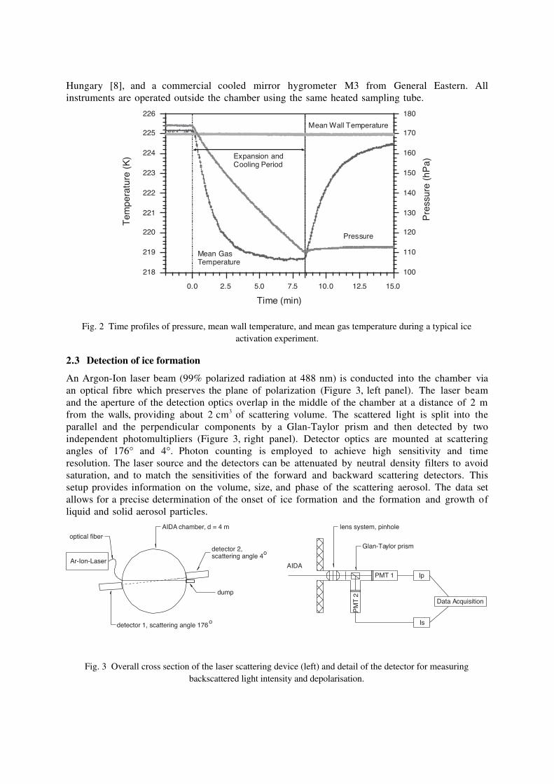
Hungary [8], and a commercial cooled mirror hygrometer M3 from General Eastern. Allinstruments are operated outside the chamber using the same heated sampling tube.

218

219

220

221

222

223

224

225

226

100

110

120

130

140

150

160

170

180

0.0 2.5 5.0 7.5 10.0 12.5 15.0

Time (min)

Pressure

Mean Wall Temperature

Mean GasTemperature

Expansion andCooling Period

Pre

ssur

e (h

Pa)

Tem

pera

ture

(K

)

Fig. 2 Time profiles of pressure, mean wall temperature, and mean gas temperature during a typical iceactivation experiment.

2.3 Detection of ice formation

An Argon-Ion laser beam (99% polarized radiation at 488 nm) is conducted into the chamber viaan optical fibre which preserves the plane of polarization (Figure 3, left panel). The laser beamand the aperture of the detection optics overlap in the middle of the chamber at a distance of 2 mfrom the walls, providing about 2 cm3 of scattering volume. The scattered light is split into theparallel and the perpendicular components by a Glan-Taylor prism and then detected by twoindependent photomultipliers (Figure 3, right panel). Detector optics are mounted at scatteringangles of 176∞ and 4∞. Photon counting is employed to achieve high sensitivity and timeresolution. The laser source and the detectors can be attenuated by neutral density filters to avoidsaturation, and to match the sensitivities of the forward and backward scattering detectors. Thissetup provides information on the volume, size, and phase of the scattering aerosol. The data setallows for a precise determination of the onset of ice formation and the formation and growth ofliquid and solid aerosol particles.

AIDAAr-Ion-Laser

dump

optical fiber

detector 1, scattering angle 176

detector 2,scattering angle 4

AIDA chamber, d = 4 m

PMT 1

PM

T 2

Ip

Is

Data Acquisition

Glan-Taylor prism

lens system, pinhole

o

o

Fig. 3 Overall cross section of the laser scattering device (left) and detail of the detector for measuringbackscattered light intensity and depolarisation.

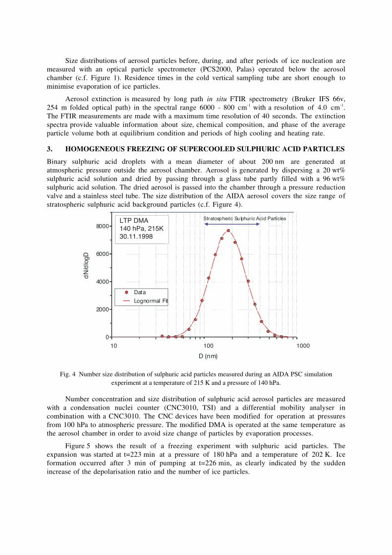
Size distributions of aerosol particles before, during, and after periods of ice nucleation aremeasured with an optical particle spectrometer (PCS2000, Palas) operated below the aerosolchamber (c.f. Figure 1). Residence times in the cold vertical sampling tube are short enough tominimise evaporation of ice particles.

Aerosol extinction is measured by long path in situ FTIR spectrometry (Bruker IFS 66v,254 m folded optical path) in the spectral range 6000 - 800 cm-1 with a resolution of 4.0 cm-1.The FTIR measurements are made with a maximum time resolution of 40 seconds. The extinctionspectra provide valuable information about size, chemical composition, and phase of the averageparticle volume both at equilibrium condition and periods of high cooling and heating rate.

3. HOMOGENEOUS FREEZING OF SUPERCOOLED SULPHURIC ACID PARTICLES

Binary sulphuric acid droplets with a mean diameter of about 200 nm are generated atatmospheric pressure outside the aerosol chamber. Aerosol is generated by dispersing a 20 wt%sulphuric acid solution and dried by passing through a glass tube partly filled with a 96 wt%sulphuric acid solution. The dried aerosol is passed into the chamber through a pressure reductionvalve and a stainless steel tube. The size distribution of the AIDA aerosol covers the size range ofstratospheric sulphuric acid background particles (c.f. Figure 4).

LTP DMA140 hPa, 215 K30.11.1998

0

2000

4000

6000

8000

10 100 1000

D (nm)

dN

/dlo

gD

Data

Lognormal Fit

Stratospheric Su lphuric Acid ParticlesLTP DMA140 hPa, 215K30.11.1998

Fig. 4 Number size distribution of sulphuric acid particles measured during an AIDA PSC simulationexperiment at a temperature of 215 K and a pressure of 140 hPa.

Number concentration and size distribution of sulphuric acid aerosol particles are measuredwith a condensation nuclei counter (CNC3010, TSI) and a differential mobility analyser incombination with a CNC3010. The CNC devices have been modified for operation at pressuresfrom 100 hPa to atmospheric pressure. The modified DMA is operated at the same temperature asthe aerosol chamber in order to avoid size change of particles by evaporation processes.

Figure 5 shows the result of a freezing experiment with sulphuric acid particles. Theexpansion was started at t=223 min at a pressure of 180 hPa and a temperature of 202 K. Iceformation occurred after 3 min of pumping at t=226 min, as clearly indicated by the suddenincrease of the depolarisation ratio and the number of ice particles.

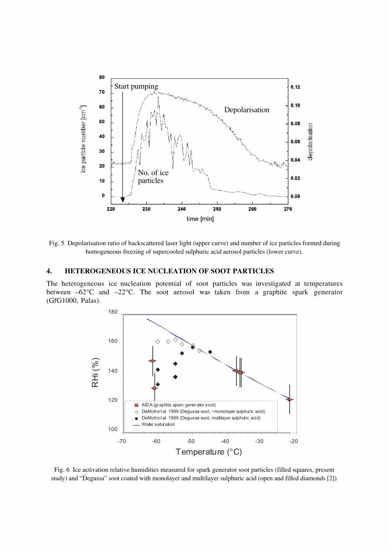
Fig. 5 Depolarisation ratio of backscattered laser light (upper curve) and number of ice particles formed duringhomogeneous freezing of supercooled sulphuric acid aerosol particles (lower curve).

4. HETEROGENEOUS ICE NUCLEATION OF SOOT PARTICLES

The heterogeneous ice nucleation potential of soot particles was investigated at temperaturesbetween –62∞C and –22∞C. The soot aerosol was taken from a graphite spark generator(GfG1000, Palas).

100

120

140

160

180

-70 -60 -30 -20

Temper-50

ature (°-40

C)

RH

i(%

)

AIDA (graphite sparc generator soot)DeMott e t al. 1999 (Degussa soot, ~monolayer sulphuric acid)DeMott e t al. 1999 (Degussa soot, multilayer sulphuric acid)Water saturation

Fig. 6 Ice activation relative humidities measured for spark generator soot particles (filled squares, presentstudy) and “Degussa” soot coated with monolayer and multilayer sulphuric acid (open and filled diamonds [2]).

Depolarisation

No. of iceparticles

Start pumping

The relative humidity with respect to ice, RHi, was calculated as function of measured icefrost point and mean gas temperature. Figure 6 shows RHi measured at the onset of ice formation.At higher temperatures liquid water seems to condense on the soot particles before ice activationoccurs (immersion freezing). At lower temperatures ice is formed significantly below the liquidwater saturation threshold. Figure 6 also depicts results from DeMott et al. [2]. Degussa soot usedin that study shows significant lowering of ice onset RHi only for multilayer sulphuric acidcoating. The GfG soot used in the AIDA experiments had not been coated with sulphuric acid.

5. SUMMARY AND CONCLUSION

In the AIDA experimental facility, ice activation experiments are performed by simulating cyclesof ice and water super- and sub-saturations, using the method of expansion-cooling. Relativehumidity can dynamically be increased in a controlled manner from ice saturation to values abovewater saturation within several minutes. First results on homogeneous freezing of super-cooledsulphuric acid particles and heterogeneous ice nucleation of soot prove the AIDA facility to bewell suited for IN studies. One of the major advantages of AIDA ice nucleation experiments is thefact that only a minor fraction of the aerosol is lost during expansion cycles. Therefore, the sameaerosol sample can be investigated in repeated activation and evaporation cycles. This opens anavenue for future experiments to study the influence of particle ageing effects (e.g. restructuring,coating) on the ice nucleation potential of relevant aerosols.

ACKNOWLEDGEMENTS

Valuable assistance by Rainer Buschbacher, Meinhard Koyro, Elisabeth Kranz, Georg Scheurig,and Claudia Tromm, is gratefully acknowledged.

REFERENCES

[1] H.R. Pruppacher, and J.D. Klett, Microphysics of clouds and precipitation (KluwerAcademic Publishers, 1997).

[2] P.J. DeMott, Y. Chen, S.M. Kreidenweis, D.C. Rogers, and D.E. Sherman, Geophys. Res.Lett. 26 (1999) 2429.

[3] K.S. Carslaw et al., Nature 391 (1998) 675.

[4] H. Mehrtens, U. von Zahn, F. Fierli, B. Nardi, and T. Deshler, Geophys. Res. Lett. 26(1999) 603.

[5] J. Schreiner, C. Voigt, A. Kohlmann, F. Arnold, K. Mauersberger, and N. Larsen, Science283 (1999) 968.

[6] A. Waibel et al., Science 283 (1999) 2064.

[7] M. Zöger et al., J. Geophys. Res. 104 (1999) 1807.

[8] M. Szakáll, Z. Bozóki, M. Krämer, N. Spelten, O. Moehler, and U. Schurath, Environ. Sci.Technol. (submitted).

THE ESF SCIENTIFIC NETWORK, SPECIAL

M.J. Rycroft1, M. Fuellekrug2, N. B. Crosby3 and A.S. Rodger4

1 Faculty of Computing Sciences and Engineering, De Montfort University, The Gateway, LeicesterLE1 9BH, U.K., Email: michael.j.rycroft@ukgateway.net2 Institute of Meteorology and Geophysics, Feldbergstrasse 47, University of Frankfurt/Main, 60323Frankfurt/Main, Germany, Email: fuellekr@geophysik.uni-frankfurt.de3 University College London, Mullard Space Science Laboratory, Holmbury St. Mary, Dorking,Surrey RH5 6NT, U.K., Email nbc@mssl.ucl.ac.uk4 British Antarctic Survey, Madingley Road, Cambridge CB3 0ET, U.K., Email: a.rodger@bas.ac.uk

AbstractIn May 1999, the European Science Foundation approved funding for theestablishment of a new Scientific Network on Space Processes and ElectricalChanges Influencing Atmospheric Layers. In this interdisciplinary area,possible links between changes of energetic charged particle fluxes and ofweather and climate occurring via electrical processes in the atmosphere arebeing investigated with a three-pronged approach, with groups being set upon:a) the AC, and DC, global atmospheric electric circuit, i.e. concerned withcharges, currents and potential differences in the atmosphere, and itselectrical conductivity,b) tropospheric and stratospheric responses to energetic charged particlesduring well-observed space weather events, and statistical studies of suchrelationships,c) Schumann resonances of the Earth-ionosphere cavity excited by tropicallightning, and sprites (upward lightning which heats and ionises the upperatmosphere at heights between 70 and 90 km).Some interesting results of collaborative experiments, data analysis, theoryand modelling obtained to date are presented. A second phase of theSPECIAL Scientific Network has been approved to run from January 2002to December 2003. Its purpose is to study the links between solar activity,magnetospheric variability, clouds, thunderstorms and lightning further.

1. BACKGROUND TO SPECIAL

The recent Intergovernmental Panel on Climate Change (IPCC 2001) identified the largest unknownsin the climate system as being the effects of a) aerosols and b) the Sun [1]. The way in which theSun affects the Earth's climate may be through direct processes (e.g., UV radiation) or throughindirect processes. Many mechanisms have been suggested; these are reviewed in a recent dedicatedissue of Space Science Reviews [2].

The Scientific Network on Space Processes and Electrical Changes Influencing AtmosphericLayers (SPECIAL) is a cross disciplinary scientific programme that addresses two key topics inclimate change, aerosols and some effects of the Sun, from a novel perspective. Approved by theEuropean Science Foundation in May 1999, SPECIAL ran until the end of 2000 [3]. Details aregiven on the website http://www.sgo.fi/SPECIAL for which T. Ulich is responsible.

In this study of space weather and Earth's weather phenomena, emphasis is placed on thephysics, and physical mechanisms, by which the two may be causally linked. The energy input todifferent layers of the atmosphere, in situ, from above and from below is considered, as is the energytransfer from one location to another. Whilst atmospheric physics generally discusses fluid dynamicsand thermodynamics and the conversion of energy from one form to another on a variety oftimescales, in SPECIAL, electrodynamics, and electricity and magnetism, are also directly involved.Thunderstorms and the global atmospheric electric circuit are significant phenomena in SPECIAL.Both linear and non-linear feedback processes may be important: negative feedback stabilises thesystem, but positive feedback leads to the amplification of an initial perturbation and, perhaps,instability and large amplitude oscillations. Threshold effects, or triggering mechanisms, whereby asmall energy input can lead to a large effect, could be significant in the physical linkages here.

SPECIAL covers a controversial, but potentially very important, area of research where severalprocesses interact in the complex laboratory which is our atmosphere and which protects us fromenergetic photons and other forms of radiation from the Sun and the cosmos beyond. In outline,SPECIAL investigates the links between changes in the fluxes of galactic cosmic rays, solar energeticcharged particles and precipitating magnetospheric charged particles and changes of the weather andclimate occurring via electrical processes in the atmosphere. The aim of SPECIAL is to improve ourscientific understanding of such topics within the Sun-Earth scenario.

The physical agents responsible for solar variability effects in the Earth's atmosphere may be a)solar ultraviolet radiation, b) charged particles (e.g., cosmic rays, solar particles or magnetosphericparticles precipitating into the atmosphere) or c) waves (tides, planetary scale waves, gravity waves,etc.; see, e.g., Arnold and Robinson [4]). Topic a) is not discussed further here because changes ofultraviolet radiation and the stratosphere form the basis of the Stratospheric Processes and their Rolein Climate (SPARC) programme. Neither is topic c) specifically considered further.

In SPECIAL, the focus is on charged particle effects, from the lowest energies (thermal; eV) inthe ionosphere, to magnetospheric (keV), solar proton (MeV) and galactic cosmic ray (GeV) effectsin the troposphere [3]. High energy charged particles reach deep into the atmosphere to deposit theirenergy, or to cause ionisation, there. They can change the electrical conductivity of the atmosphere(which is due to ions); the atmosphere is a good insulator near the Earth's surface, but is highlyconducting near the ionosphere, where the very mobile electrons determine the conductivity.

2. SOME RESULTS RELEVANT TO THE SPECIAL PROGRAMME

Roederer [5] presented a valuable review of both observational claims and possible mechanisms forsolar variability effects on climate. Atmospheric ionisation and the global electric circuit are featuredhere. In 1959, Ney [6] showed observationally that at solar maximum the tropospheric andstratospheric ionisation was less than at solar minimum. We now know that this 11 year solar cycleeffect is due to the enhanced scattering of galactic cosmic rays by irregularities of the interplanetarymagnetic field near solar maximum, the mechanism which is also responsible for Forbush decreases.Cosmic ray flux variations may also cause variations of aerosol production in the atmosphere and ofcloud droplet nucleation. The change of atmospheric ionisation is sizeable, ranging from ~5% to~50%: the effect is more marked at higher altitudes and higher latitudes. Bazilevskaya et al. [7] haverecently reviewed this topic comprehensively.

In the same Golden Jubilee issue of the journal, Rycroft et al. [8] have considered the globalatmospheric electric circuit. Their Fig.5 shows the upward current above a typical thundercloud,~1.3A [9], for about the thousand thunderstorms that are active at any one time, on average. That

charges the ionosphere to a potential of ~ +250 kV with respect to the Earth's surface. The returncurrent J ~ 2 pA m-2 flows through the fair weather atmosphere remote from thunderstorms; it isbelieved that these return currents close through the land/ocean surface and the lowest part of theatmosphere below thunderclouds, but electrified shower clouds could also be important [10].

Following a Forbush decrease, the tropospheric conductivity could decrease by ~10%. If J isunchanged, an increase by ~10% in the fair weather electric field near the Earth's surface, E ~ 130 Vm-1, could be expected. However, it is not easy to detect that in a noisy signal due to localmeteorological effects. Markson [11] indicated that a 10% change of ground level cosmic radiationwas associated with a 10-20% variation of ionospheric potential.

By Poisson's equation and Gauss' theorem, which relate the charge density to the electric fielddistribution through the atmosphere with its conductivity gradient, charged layers may exist nearcloud tops. Here, electroscavenging could occur and ice may be produced [12], leading to theformation of clouds. Clouds exert a profound influence on radiative forcing and the radiationbalance of the atmosphere, and hence on the weather and climate [1, 12].

Pudovkin and Veretenenko [13] claim that 1 or 2 days after a Forbush decrease in winter thecloudiness at geographic latitudes between 60∞ and 64∞ is about 7% (1 or 2 standard deviations) lessthan usual. Using the Student's t-test, this is significant at the 98% level. They observe no variationsat middle latitudes (~50∞). Marsh and Svensmark [14] find that the total cloud cover over southernhemisphere oceans derived from satellite observations is 1.5% less at solar maximum than at solarminimum when the cosmic ray flux at the mid-latitude Climax station (in Colorado) is ~10% less.Following a Forbush decrease or solar proton event, changes of the atmospheric circulation at 30 hPa(~24 altitude km) and 500 hPa (~5 km) have been discussed by Gabis and Troshichev [15].

King [16] showed that the length of the growing season in Southern Scotland seems to exhibitthe 11 year solar cycle variation. If real, this effect is important for the agricultural economies ofnations worldwide.

Kristjansson and Kristiansen [17] presented a possible causal mechanism between increasedsolar activity, reduced cosmic ray flux and reduced cloud cover, and - perhaps - a warmer climate.On the other hand, Ney [6] speculated that a reduced cosmic ray flux would lead to decreasedatmospheric ionisation and - perhaps - increased thunderstorm activity and a cooler climate. Williams[18] and Price [19] suggested that increased thunderstorm activity is associated with global warming(see also [8, 20]).

3. THE SPECIAL PROGRAMME

The planning and carrying out of the work in the framework of SPECIAL have been done in threedistinct groups [3]. These three groups, each of a reasonable size, cover:

a) the AC, and DC, global atmospheric electric circuit, i.e. concerned with charges, electriccurrents and potential differences in the atmosphere, and its electrical conductivity.

b) tropospheric and stratospheric responses to energetic charged particle fluxes during wellobserved space weather events, and also statistical studies of such relationships,

c) Schumann resonances of the Earth-ionosphere cavity (~8 Hz fundamental) excited bytropical lightning, and also sprites (upward lightning which heats and ionises the upper atmosphere ataround 70 to 90 km altitude).

The SPECIAL Scientific Network has held two meetings which engendered considerable cross-disciplinary research and discussion. Some new collaborations have been established and the firstresults are beginning to be published. For example, Neubert et al. [21] have conducted the firstEuropean sprite campaign. Rodger et al. [22] have recently shown that sprites could double thenight-time ionospheric electron concentration at 90 km altitude. Egorova et al. [23] and Lam andRodger [24] have been exploring the extent to which Forbush decreases cause changes in thetroposphere over the Antarctic in the polar night. Schlegel et al. [25] have demonstrated some solarcycle variations in lightning occurrence over Germany. However, it is equally challenging to explainthe lack of a solar cycle effect over Austria.

Another relevant recent result is that of Schlegel and Fuellekrug [26], who showed thationisation at the upper boundary of the Earth-ionosphere cavity increases during solar proton events.This is responsible for an observed increase (~0.1 Hz) of the fundamental resonant frequency (seealso [18, 20]), and a decrease of up to 10% in its damping. In the same Golden Jubilee issuementioned earlier, Barr et al. [27] comprehensively review the topic of ELF/VLF radio wavephenomena, including Schumann resonances; Rodger and Jarvis [28] consider some important topicsof ionospheric research, highlighting long term changes and areas of study still required before betterlong term predictions can be made.

A second phase of SPECIAL has recently been approved by the European Science Foundation.The work of the three groups will thus continue until the end of December 2003, the objectives beingto investigate the links between solar activity, magnetospheric variability, clouds, thunderstorms andlightning further. This interdisciplinary arena is especially challenging.

4. REFERENCES

[1] Houghton J.T., Ding Y., Griggs D.J., Noguer M., van der Linden P.J. and Xiaosu D. (ed.),Climate change 2001: The scientific basis, Cambridge University Press, pp.944, 2001.

[2] Friis-Christensen E., Frohlich C., Haigh J.D., Schlusser M. and von Steiger R. (ed.), SolarVariability and Climate, Space Science Reviews, Vol. 94, 1-427, 2000.

[3] Crosby N.B. and Rycroft M.J., SPECIAL: an interdisciplinary ESF network on space weatherand the Earth's weather, Proc. 1st Solar and Space Weather Euroconference, 'The Solar Cycleand Terrestrial Climate', ESA SP-463, 219-221, 2000.

[4] Arnold N.F. and Robinson T.R., Solar cycle changes to planetary wave propagation and theirinfluence on the middle atmosphere circulation, Ann. Geophysicae, Vol. 16, 69-76, 1998.

[5] Roederer J.G., Solar variability effects on climate, ESF Workshop, Solar Output and Climateduring the Holocene, Bologna, Italy, April, 1993.

[6] Ney E.P., Cosmic radiation and the weather, Nature, Vol. 183, 451-452, 1959.

[7] Bazilevskaya G.A., Krainev M.B. and Makhmutov V.S., Effects of cosmic rays on the Earth'senvironment, J. Atmos. Sol.-Terr. Phys., Vol. 62, 1577-1586, 2000.

[8] Rycroft M.J., Israelsson S. and Price C., The global atmospheric electric circuit, solar activityand climate change, J. Atmos. Sol.-Terr. Phys., Vol. 62, 1563-1576, 2000.

[9] Stergis G.G., Rein G.C. and Kangas T., Electric field measurements above thunderstorms, J.Atmos. Terr. Phys., Vol. 11, 83-90, 1957.

[10] Markson R., Private communication, 2001.

[11] Markson R., Modulation of the Earth's electric field by cosmic radiation, Nature, Vol. 291,304-308, 1981.

[12] Tinsley B.A., Influence of solar wind on the global electric circuit, and inferred effects oncloud microphysics, temperature, and dynamics in the troposphere, in [2], Solar Variabilityand Climate (ed. Friis-Christensen E., Frohlich C., Haigh J.D., Schlusser M. and von SteigerR.), Kluwer Academic Publishers, Dordrecht, The Netherlands, 231-258, 2000.

[13] Pudovkin M.I. and Veretenenko S.V., Variations of the cosmic rays as one of the possiblelinks between the solar activity and the lower atmosphere, Adv. Space Res., Vol. 17, (11)161-(11)164, 1996.

[14] Marsh N. and Svensmark H., Cosmic rays, clouds and climate, in [2], Space Science Reviews,Vol. 94, 215-230, 2000.

[15] Gabis I.P. and Troshichev O.A., Influence of short-term changes in solar activity on baricfield perturbations in the stratosphere and troposphere, J. Atmos. Sol.-Terr. Phys., Vol. 62,725-735, 2000.

[16] King J.W., Solar radiation changes and the weather, Nature, Vol. 245, 443-446, 1973.

[17] Kristjannson J.E. and Kristiansen, J., Is there a cosmic ray signal in recent variations in globalcloudiness and cloud radiative forcing? J. Geophys. Res., Vol. 105, 11851-11863, 2000.

[18] Williams E.R., The Schumann resonance: a global thermometer, Science, Vol. 256, 1184-1187, 1992.

[19] Price C., Global surface temperatures and the atmospheric electrical circuit, Geophys. Res.Lett., Vol. 20, 1363-1366, 1993.

[20] Price C., Evidence for a link between global lightning activity and upper tropospheric watervapour, Nature, Vol. 406, 290-293, 2000.

[21] Neubert T., Allin T.H., Stenback-Nielsen H. and Blanc E., Sprites over Europe, Geophys. Res.Lett., Vol. 28, 3585-3588, 2001.

[22] Rodger C.J., Cho M., Clilverd M.A. and Rycroft M.J., Lower ionospheric modification bylightning-EMP: simulation of the night ionosphere over the United States, Geophys. Res.Lett.,Vol. 28, 199-202, 2001.

[23] Egorova L.V., Vovk V.Y. and Troshichev O.A., Influence of variations of the cosmic rays onatmospheric pressure and temperature in the Southern geomagnetic pole region, J. Atmos.Sol.-Terr. Phys., Vol. 62, 955-966, 2000.

[24] Lam M.M. and Rodger A.S., The effects of Forbush decreases on tropospheric parametersover the Antarctic, J. Atmos. Sol.-Terr. Phys. (in press).

[25] Schlegel K., Diendorfer D., Thern S. and Schmidt S., Thunderstorms, lightning and solaractivity - Middle Europe, J. Atmos. Sol.-Terr. Phys., Vol. 63, 1715-1728, 2001.

[26] Schlegel K. and Fuellekrug M., Schumann resonance parameter changes during high-energyparticle precipitation, J. Geophys. Res., Vol. 104, 10111-10118, 1999.

[27] Barr R., Jones D.L. and Rodger C.J., ELF and VLF radio waves, J. Atmos. Sol.-Terr.Phys.,Vol. 62, 1689-1718, 2000.

[28] Rodger A.S. and Jarvis M.J., Ionospheric research 50 years ago, today and tomorrow, J.Atmos. Sol-Terr. Phys., Vol. 62, 1629-1645, 2000.

CLOUD: A PARTICLE BEAM FACILITY TO INVESTIGATE THEINFLUENCE OF COSMIC RAYS ON CLOUDS

Jasper KirkbyCERN, Geneva, Switzerland

AbstractPalaeoclimatic data provide extensive evidence for solar forcing of the cli-mate during the Holocene1 and the last ice age, but the underlying mecha-nism remains a mystery. However recent observations suggest that cosmicrays may play a key role. Satellite data have revealed a surprising correla-tion between cosmic ray intensity and the fraction of the Earth covered by lowclouds [1, 2]. Since the cosmic ray intensity is modulated by the solar wind,this may be an important clue to the long-sought mechanism for solar-climatevariability. In order to test whether cosmic rays and clouds are causally linkedand, if so, to understand the microphysical mechanisms, a novel experimentknown as CLOUD2 has been proposed [3]–[5]. CLOUD proposes to inves-tigate ion-aerosol-cloud microphysics under controlled laboratory conditionsusing a beam from a particle accelerator, which provides a precisely adjustableand measurable artificial source of cosmic rays. The heart of the experimentis a precision cloud chamber that recreates cloud conditions throughout theatmosphere.

1 INTRODUCTION

That there is a causal connection between the observed variations in the forces of the Sun,the terrestrial magnetic field, and the meteorological elements has been the conclusion ofevery research into this subject for the past 50 years. The elucidation of exactly what theconnection is and the scientific proof of it is to be classed among the most difficult problemspresented in terrestrial physics. The evidence adduced in favor of this conclusion is on thewhole of a cumulative kind, since the direct sequence of cause and effect is so far masked inthe complex interaction of the many delicate forces in operation as to render its immediatemeasurement quite impossible in the present state of science.

F.H. BigelowUS Dept. Agriculture Weather Bureau

Bulletin No.21, 1898

This quotation [6] is from an article written over a century ago and yet it could be taken almostwholly from a contemporary paper. The observation that warm weather seems to coincide with highsunspot counts and cool weather with low sunspot counts was made as long ago as two hundred yearsby the astronomer William Herschel [7] who noticed that the price of wheat in England was lowerwhen there were many sunspots, and higher when there were few. The most well-known example ofa solar-climate effect is known as the Maunder Minimum [8], the period between 1645 and 1715—which ironically almost exactly coincides with the reign of Louis XIV, le Roi Soleil, 1643–1715—duringwhich there was an almost complete absence of sunspots (Fig. 1). This marked the most pronounced ofseveral prolonged cold spells in the period between about 1450 and 1890 which are collectively knownas the Little Ice Age. During this period the River Thames in London regularly froze across and fairs

1The Holocene is the present interglacial period—the previous 11.5 kyr since the end of the last ice age.2CLOUD is an acronym for Cosmics Leaving OUtdoor Droplets.

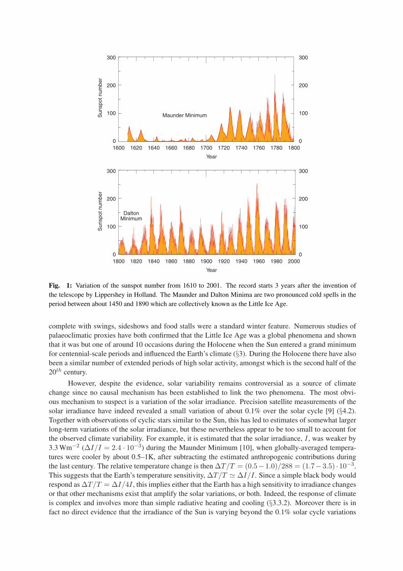
0

100

200

300

0

100

200

300

Sun

spot

num

ber

Year

1800 1820 1840 1860 1880 1900 1920 1940 1960 1980 2000

0

100

200

300

0

100

200

300

Sun

spot

num

ber

Year

1600 1620 1640 1660 1680 1700 1720 1740 1760 1780 1800

Maunder Minimum

DaltonMinimum

Fig. 1: Variation of the sunspot number from 1610 to 2001. The record starts 3 years after the invention ofthe telescope by Lippershey in Holland. The Maunder and Dalton Minima are two pronounced cold spells in theperiod between about 1450 and 1890 which are collectively known as the Little Ice Age.

complete with swings, sideshows and food stalls were a standard winter feature. Numerous studies ofpalaeoclimatic proxies have both confirmed that the Little Ice Age was a global phenomena and shownthat it was but one of around 10 occasions during the Holocene when the Sun entered a grand minimumfor centennial-scale periods and influenced the Earth’s climate (§3). During the Holocene there have alsobeen a similar number of extended periods of high solar activity, amongst which is the second half of the20th century.

However, despite the evidence, solar variability remains controversial as a source of climatechange since no causal mechanism has been established to link the two phenomena. The most obvi-ous mechanism to suspect is a variation of the solar irradiance. Precision satellite measurements of thesolar irradiance have indeed revealed a small variation of about 0.1% over the solar cycle [9] (§4.2).Together with observations of cyclic stars similar to the Sun, this has led to estimates of somewhat largerlong-term variations of the solar irradiance, but these nevertheless appear to be too small to account forthe observed climate variability. For example, it is estimated that the solar irradiance, I , was weaker by3.3 Wm−2 (∆I/I = 2.4 · 10−3) during the Maunder Minimum [10], when globally-averaged tempera-tures were cooler by about 0.5–1K, after subtracting the estimated anthropogenic contributions duringthe last century. The relative temperature change is then ∆T/T = (0.5− 1.0)/288 = (1.7− 3.5) · 10−3.This suggests that the Earth’s temperature sensitivity, ∆T/T ∆I/I . Since a simple black body wouldrespond as ∆T/T = ∆I/4I , this implies either that the Earth has a high sensitivity to irradiance changesor that other mechanisms exist that amplify the solar variations, or both. Indeed, the response of climateis complex and involves more than simple radiative heating and cooling (§3.3.2). Moreover there is infact no direct evidence that the irradiance of the Sun is varying beyond the 0.1% solar cycle variations

(which can be quantitatively well-explained by sunspot darkening and facular brightening of the pho-tosphere). So the magnitude of the long-term change in solar irradiance—if any—is speculative. Thephysical mechanism or mechanisms for solar-climate variability therefore remain a mystery.

However, the recent observation of correlations between the galactic cosmic ray (GCR) intensityand the fraction of Earth covered by low clouds [1, 2] (§2.1) may provide an important clue. Cloudscover a large fraction of the Earth’s surface—a global annual mean of about 65%—and exert a strong netcooling effect of about 30 Wm−2, so long-term variations of only a few per cent could have a significanteffect on the Earth’s climate. Since the GCR intensity is modulated by the solar wind, a GCR-cloud linkcould provide a sufficient amplifying mechanism for solar-climate variability. This would constitute anew solar indirect contribution to climate change, in addition to the direct contribution from irradiancechanges (§3.3.5).

If a causal connection between GCR intensity and low cloud cover were to be confirmed, it couldhave profound consequences for our understanding of the solar contributions to the current global warm-ing. During the 20th century the Sun’s magnetic activity increased dramatically and the solar wind morethan doubled in strength [11] (§3.3.1). As a consequence, the mean GCR intensity on Earth diminishedby about 15%. The implied reduction in low cloud cover by about 1.3% absolute could have givenrise to a radiative forcing of about +0.8 Wm−2 (3.3 · 10−3), which is comparable to the estimated totalanthropogenic forcing of about +1.3 Wm−2 (§3.3.5).

We can look further back in time for evidence of solar forcing3 of the climate. Detailed recordsof the magnetic variability of the Sun are preserved in the light radio isotope archives, notably the 14Ccontent of tree-rings (for about the last 10 kyr) and the 10Be concentrations in ice-cores from Greenlandand Antarctica (about 250 kyr) (§3.1.1). The light radio isotopes are produced by GCRs interacting withnitrogen, oxygen and argon nuclei in the atmosphere, and so they are a direct measure the prevailingGCR intensity. These records show the Sun to be a variable star, with both quasi-cyclic activity (11, 88,208 yr. . . ) and also periods of ‘grand-minima’ occurring on millennial-scale intervals. Diverse palaeo-climatic records have also shown that the Earth’s climate was not stable in the past and that large changeshave occurred naturally. Comparisons between the solar and palaeoclimatic records reveal unmistakableevidence for a solar forcing of the climate (§3.2–§3.3).

However, in the absence of an established physical mechanism, even the evidence for solar-climatecorrelations accumulated in studies over the last two hundred years has not proved cause and effect. Butnow—and perhaps for the first time—we have a definite hypothesis for the mechanism that can be testedexperimentally, namely: are cosmic rays affecting cloud formation? Since the energy flux from cosmicrays is tiny—about the same as that from starlight, and only a few parts per billion compared with thesolar irradiance—a strong amplification mechanism would be required, i.e. some microphysical propertyor properties of clouds must be very sensitive to the ionisation or radicals produced by GCRs. Although afrequent criticism of the GCR-cloud hypothesis has been the absence of any microphysical mechanism,there are in fact several candidates, associated with aerosols, ice particles and cloud electricity (§4).However since none of these mechanisms is firmly established, they must tested experimentally.

How can this best be done? In the atmosphere it is hard to establish cause and effect since it isdifficult to measure all the variables and essentially impossible to adjust them. For these reasons theCLOUD experiment [3]–[5] (§5) proposes to perform the necessary measurements under controlled con-ditions in the laboratory. CLOUD plans to use a particle beam from an accelerator to provide a preciselycontrollable source of relativistic ionising radiation that closely duplicates cosmic rays in the atmosphere(§5.4). Processes can be studied with beams of varying intensity around naturally-occurring levels, andalso with no beam present. The beam will pass through an expansion cloud chamber (§5.3.1) and a re-actor chamber where the atmosphere is duplicated by moist air charged with selected aerosols and tracecondensable vapours. The cloud chamber dynamically simulates the thermodynamic conditions, electric

3A climate forcing is a perturbation of the Earth’s radiative energy balance, with the convention that a positive forcing leadsto a warming, and a negative forcing to a cooling.

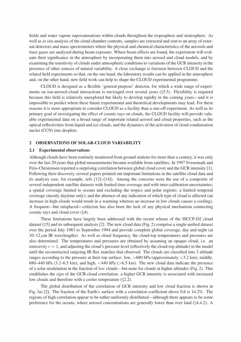
fields and water vapour supersaturations within clouds throughout the troposphere and stratosphere. Aswell as in situ analysis of the cloud chamber contents, samples are extracted and sent to an array of exter-nal detectors and mass spectrometers where the physical and chemical characteristics of the aerosols andtrace gases are analysed during beam exposure. Where beam effects are found, the experiment will eval-uate their significance in the atmosphere by incorporating them into aerosol and cloud models, and byexamining the sensitivity of clouds under atmospheric conditions to variations of the GCR intensity in thepresence of other sources of natural variability. A close exchange is foreseen between CLOUD and therelated field experiments so that, on the one hand, the laboratory results can be applied in the atmosphereand, on the other hand, new field work can help to shape the CLOUD experimental programme.

CLOUD is designed as a flexible ‘general-purpose’ detector, for which a wide range of experi-ments on ion-aerosol-cloud interactions is envisaged over several years (§5.5). Flexibility is requiredbecause this field is relatively unexplored but likely to develop rapidly in the coming years—and it isimpossible to predict where these future experimental and theoretical developments may lead. For thesereasons it is more appropriate to consider CLOUD as a facility than a one-off experiment. As well as itsprimary goal of investigating the effect of cosmic rays on clouds, the CLOUD facility will provide valu-able experimental data on a broad range of important related aerosol and cloud properties, such as theoptical reflectivities from liquid and ice clouds, and the dynamics of the activation of cloud condensationnuclei (CCN) into droplets.

2 OBSERVATIONS OF SOLAR-CLOUD VARIABILITY

2.1 Experimental observations

Although clouds have been routinely monitored from ground stations for more than a century, it was onlyover the last 20 years that global measurements became available from satellites. In 1997 Svensmark andFriis-Christensen reported a surprising correlation between global cloud cover and the GCR intensity [1].Following their discovery, several papers pointed out important limitations in the satellite cloud data andits analysis (see, for example, refs. [12]–[14]). Among the concerns were the use of a composite ofseveral independent satellite datasets with limited time coverage and with inter-calibration uncertainties;a spatial coverage limited to oceans and excluding the tropics and polar regions; a limited temporalcoverage (mostly daytime only); and the absence of any indication of which type of cloud is affected (anincrease in high clouds would result in a warming whereas an increase in low clouds causes a cooling).A frequent—but misplaced—criticism has also been the lack of any physical mechanism connectingcosmic rays and cloud cover (§4).

These limitations have largely been addressed with the recent release of the ISCCP-D2 clouddataset [15] and its subsequent analysis [2]. The new cloud data (Fig. 2) comprise a single unified datasetover the period July 1983 to September 1994 and provide complete global coverage, day and night (at10–12 µm IR wavelengths). As well as cloud frequency, the cloud-top temperatures and pressures arealso determined. The temperatures and pressures are obtained by assuming an opaque cloud, i.e. anemissivity ε = 1, and adjusting the cloud’s pressure level (effectively the cloud-top altitude) in the modeluntil the reconstructed outgoing IR flux matches that observed. The clouds are classified into 3 altituderanges according to the pressure at their top surface: low, >680 hPa (approximately <3.2 km); middle,680–440 hPa (3.2–6.5 km); and high, <440 hPa (>6.5 km). The new cloud data indicate the presenceof a solar modulation in the fraction of low clouds—but none for clouds at higher altitudes (Fig. 2). Thisestablishes the sign of the GCR-cloud correlation: a higher GCR intensity is associated with increasedlow clouds and therefore with a cooler temperature (§2.2).

The global distribution of the correlation of GCR intensity and low cloud fraction is shown inFig. 3a) [2]. The fraction of the Earth’s surface with a correlation coefficient above 0.6 is 14.2%. Theregions of high correlation appear to be rather uniformly distributed—although there appears to be somepreference for the oceans, where aerosol concentrations are generally lower than over land (§4.4.2). A

Cha

nge

in c

loud

frac

tion

(%) a) High clouds

Cha

nge

in c

loud

frac

tion

(%) b) Middle clouds

Cha

nge

in c

loud

frac

tion

(%)

Cha

nge

in c

osm

ic r

ays

(%)

c) Low clouds

cloudssolar irradiancecosmic rays (>13GeV)

cloudscosmic rays (>13GeV)

cloudscosmic rays (>13GeV)

Cha

nge

in s

olar

irra

dian

ce (

%)

-0.05

-0.10

0.10

0.05

0

Year1985 1990 1995

Year1985 1990 1995

Year1985 1990 1995

-1

0

1

2

-1

0

1

2

-1

0

1

2

-10

-5

5

0

10

Cha

nge

in c

osm

ic r

ays

(%)

-10

-5

5

0

10

Cha

nge

in c

osm

ic r

ays

(%)

-10

-5

5

0

10

Fig. 2: Monthly mean values for the global absolute variations of infra red (IR) cloud coverage for a) high (cloud-top pressure <440 hPa), b) middle (440–680 hPa), and c) low (>680 hPa) clouds (solid lines) (adapted fromrefs. [2] and [16]). The ISCCP-D2 cloud data are obtained at infra-red (IR) wavelengths (10–12 µm) and havecomplete global coverage, day and night. The variations, over this period, of cosmic ray intensity (dashed line;13 GeV/c rigidity cutoff) and solar irradiance (dotted line in lowest panel; note inverted scale) are also indicated.The mean global cloud fraction over this period for high, middle and low IR clouds is 13.5%, 19.9%, and 28.0%respectively. The cloud measurements are obtained from the ISCCP-D2 IR dataset [15].

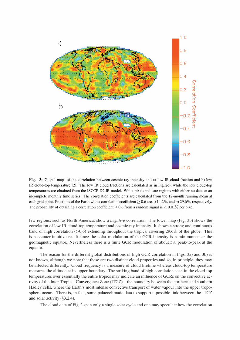
Fig. 3: Global maps of the correlation between cosmic ray intensity and a) low IR cloud fraction and b) lowIR cloud-top temperature [2]. The low IR cloud fractions are calculated as in Fig. 2c), while the low cloud-toptemperatures are obtained from the ISCCP-D2 IR model. White pixels indicate regions with either no data or anincomplete monthly time series. The correlation coefficients are calculated from the 12-month running mean ateach grid point. Fractions of the Earth with a correlation coefficient ≥ 0.6 are a) 14.2%, and b) 29.6%, respectively.The probability of obtaining a correlation coefficient ≥ 0.6 from a random signal is < 0.01% per pixel.

few regions, such as North America, show a negative correlation. The lower map (Fig. 3b) shows thecorrelation of low IR cloud-top temperature and cosmic ray intensity. It shows a strong and continuousband of high correlation (>0.6) extending throughout the tropics, covering 29.6% of the globe. Thisis a counter-intuitive result since the solar modulation of the GCR intensity is a minimum near thegeomagnetic equator. Nevertheless there is a finite GCR modulation of about 5% peak-to-peak at theequator.

The reason for the different global distributions of high GCR correlation in Figs. 3a) and 3b) isnot known, although we note that these are two distinct cloud properties and so, in principle, they maybe affected differently. Cloud frequency is a measure of cloud lifetime whereas cloud-top temperaturemeasures the altitude at its upper boundary. The striking band of high correlation seen in the cloud-toptemperatures over essentially the entire tropics may indicate an influence of GCRs on the convective ac-tivity of the Inter Tropical Convergence Zone (ITCZ)—the boundary between the northern and southernHadley cells, where the Earth’s most intense convective transport of water vapour into the upper tropo-sphere occurs. There is, in fact, some palaeoclimatic data to support a possible link between the ITCZand solar activity (§3.2.4).

The cloud data of Fig. 2 span only a single solar cycle and one may speculate how the correlation

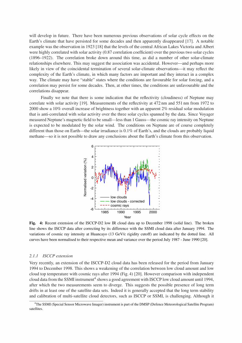
will develop in future. There have been numerous previous observations of solar cycle effects on theEarth’s climate that have persisted for some decades and then apparently disappeared [17]. A notableexample was the observation in 1923 [18] that the levels of the central African Lakes Victoria and Albertwere highly correlated with solar activity (0.87 correlation coefficient) over the previous two solar cycles(1896–1922). The correlation broke down around this time, as did a number of other solar-climaterelationships elsewhere. This may suggest the association was accidental. However—and perhaps morelikely in view of the coincidental termination of several solar-climate observations—it may reflect thecomplexity of the Earth’s climate, in which many factors are important and they interact in a complexway. The climate may have “stable” states where the conditions are favourable for solar forcing, and acorrelation may persist for some decades. Then, at other times, the conditions are unfavourable and thecorrelations disappear.

Finally we note that there is some indication that the reflectivity (cloudiness) of Neptune maycorrelate with solar activity [19]. Measurements of the reflectivity at 472 nm and 551 nm from 1972 to2000 show a 10% overall increase of brightness together with an apparent 2% residual solar modulationthat is anti-correlated with solar activity over the three solar cycles spanned by the data. Since Voyagermeasured Neptune’s magnetic field to be small—less than 1 Gauss—the cosmic ray intensity on Neptuneis expected to be modulated by the solar wind. The conditions on Neptune are of course completelydifferent than those on Earth—the solar irradiance is 0.1% of Earth’s, and the clouds are probably liquidmethane—so it is not possible to draw any conclusions about the Earth’s climate from this observation.

1985 1990 1995 2000

Nor

mal

ised

var

iatio

n (%

)

-6

-4

-2

0

2

4

6

low cloudslow clouds - correctedcosmic rays

Year

Fig. 4: Recent extension of the ISCCP-D2 low IR cloud data up to December 1998 (solid line). The brokenline shows the ISCCP data after correcting by its difference with the SSMI cloud data after January 1994. Thevariations of cosmic ray intensity at Huancayo (13 GeV/c rigidity cutoff) are indicated by the dotted line. Allcurves have been normalised to their respective mean and variance over the period July 1987 - June 1990 [20].

2.1.1 ISCCP extension

Very recently, an extension of the ISCCP-D2 cloud data has been released for the period from January1994 to December 1998. This shows a weakening of the correlation between low cloud amount and lowcloud top temperature with cosmic rays after 1994 (Fig. 4) [20]. However comparison with independentcloud data from the SSMI instrument4 shows a good agreement with ISCCP low cloud amount until 1994,after which the two measurements seem to diverge. This suggests the possible presence of long termdrifts in at least one of the satellite data sets. Indeed it is generally accepted that the long term stabilityand calibration of multi-satellite cloud detectors, such as ISCCP or SSMI, is challenging. Although it

4The SSMI (Special Sensor Microwave Imager) instrument is part of the DMSP (Defence Meteorological Satellite Program)satellites.

is not possible to resolve these discrepancies at present, an estimate of the uncertainties in the drift canbe evaluated from the difference in the long term trends of the ISCCP and SSMI data. One limit is tocorrect the ISCCP cloud data after 1990 in direction and magnitude by its difference with the SSMIdata, assuming the two datasets agree over the period 1987–1990. This is shown in Fig. 4 and indicatesa good correlation between low cloud amount and cosmic rays over the full period of available clouddata (1983-1998). The uncertainties in cloud amount for the period after 1994 appear to be too large atpresent to draw any conclusion on either the absence or presence of a correlation with the GCR intensity.

2.2 Cloud radiative forcing

The observed variation of low cloud cover over the solar cycle of about 1.7% absolute corresponds to6.0% relative. Since measurements by the Earth Radiation Budget Experiment (ERBE) indicate that lowclouds contribute a global annual mean radiative forcing of about -17 Wm−2 (Table 1) this implies thecloud modulation corresponds to about +1.0 Wm−2, solar minimum-to-maximum. This is about a factor5 larger than the solar cycle irradiance forcing at the Earth’s surface (0.2 Wm−2; §3.3.3), and in phase.

Table 1: Global annual mean forcing due to various types of clouds, from the Earth Radiation Budget Experiment(ERBE) [21].

Parameter High clouds Middle clouds Low clouds Total

Thin Thick Thin Thick All

Global fraction (%) 10.1 8.6 10.7 7.3 26.6 63.3

Forcing (relative to clear sky):

Albedo (SW radiation) (Wm−2) -4.1 -15.6 -3.7 -9.9 -20.2 -53.5

Outgoing LW radiation (Wm−2) 6.5 8.6 4.8 2.4 3.5 25.8

Net forcing (Wm−2) 2.4 -7.0 1.1 -7.5 -16.7 -27.7

3 RECORD OF SOLAR-GCR-CLIMATE CHANGE

3.1 Solar and palaeoclimatic records

3.1.1 Solar and GCR records

The flux of galactic cosmic rays reaching the Earth’s atmosphere is modulated by variations of the helio-spheric magnetic field and of the Earth’s geomagnetic field. During times of high solar activity (sunspotmaximum) there is an increase of the open magnetic flux and of the magnetic irregularities carried outinto the heliosphere by the solar wind. These magnetic fields scatter the low-energy component of theincoming GCRs (below a few tens of GeV) and, in consequence, the flux reaching Earth is reduced. Theglobal average modulation of the GCR intensity over the solar cycle is about 15%, but larger variationsoccur on longer timescales. During a reversal of the Earth’s dipole field, for example, it is estimated thatthe global GCR rate is enhanced by about a factor 2.5 relative to the present values.

An exquisite record of the variations of GCR intensity over the past 250 millennia is preservedin the light radio isotope records in ice cores [22]. These provide an essentially direct measurementof the prevailing GCR intensity and hence are a direct indication of variations of the solar magneticactivity. They are also frequently used as a proxy for putative changes of solar irradiance, althoughthere exists no direct evidence for long-term variations of the solar irradiance. The light radio-isotopesare produced in spallation interactions of GCRs on nitrogen, oxygen and argon nuclei in the atmosphere.The two radioisotopes with the highest production rates are 14C (half life = 5730±40 yr and global mean

production rate ∼2.0 atoms cm−2s−1) and 10Be (1.5 Myr; ∼1.8×10−2 atoms cm−2s−1). The third mostabundant isotope is 36Cl, which is produced from GCR interactions with Ar nuclei (300 kyr; ∼1.9×10−3

atoms cm−2s−1).

The 14C is rapidly oxidised to 14CO2. The turnover time of CO2 in the atmosphere is quite short—about 4 years—mostly by absorption in the oceans and assimilation in living plants. However, because ofrecirculation between the oceans and the atmosphere, changes in the 14C fraction on timescales less thana few decades are smoothed out. Plant material originally contains the prevailing atmospheric fractionof 14C and, subsequently, since the material is not recycled into the atmosphere, the fraction decreaseswith the characteristic half life of 14C. By analysing the 14C content in the rings of long-lived trees suchas the California bristlecone pine, a continuous yearly record of GCR intensity over the last 10–15 kyrhas been assembled.

In the case of 10Be, after production it rapidly attaches to aerosols and follows the motion ofthe surrounding air masses. Since the production of 10Be follows the intensity profile of the cosmic rayhadronic showers, about 2/3 is produced in the stratosphere and 1/3 in the troposphere, globally averaged.Due to the tropopause barrier, aerosols in the stratosphere take about 1–2 years to settle on the Earth’ssurface, whereas the mean residence time in the troposphere is only about a week. If the sedimentationoccurs in the form of snow in a permanently frozen and stable region such as Greenland or Antarcticathen the subsequent compacted ice preserves a temporal record in layers according to their depth.

The measured variations of the light radionuclides are the product of two processes: 1) the produc-tion rate and 2) system effects i.e. transport, precipitation and exchange processes between the differentreservoirs. Since the system effects are quite different for 14C and 10Be, it has been possible to reliablydetermine the production rates, and hence the GCR intensities. An advantage of 14C is that it is well-mixed before storage in the tree-ring archives. In contrast, the short residence time of the tropospheric10Be fraction means that the measured concentrations are subject to possible variations of precipitationrate and of wind directions in carrying the radionuclide from where it is produced to where it is sedi-mented as snow. However, by using a minimum sample period of 1 or 2 years, the effects of variations oftransport direction and efficiency are minimised. Since 10Be is not recycled into the atmosphere, it hasthe important advantages of being able to record relatively short-term changes in the GCR intensity, anda freedom from uncertainties due to variations in the recycling processes.

3.1.2 Palaeoclimatic records

Many ingenious proxies have been developed to reconstruct the climate prior to the last two centuries,for which instrumental records are available. Cultural records over about the last millennium are animportant source since humans are sensitive to climate change, especially when prolonged drought, coldor flooding is involved. These sources include documents recording the dates when the first cherryblossoms appeared each spring in China, as well as records of the grape harvests in Europe. Otherrecords (with their approximate time span BP 5 in parentheses) are corals (400 yr), tree rings (10 kyr),mosses (10 kyr), pollen (1 Myr), ice cores (250 kyr), ocean sediments (>1 Myr) and geomorphology(3 Byr).

Ice cores are an especially valuable record of past climate [22]. As well as the solar-GCR recorddescribed above, the trapped gases preserve the atmospheric composition at earlier times, layer thick-nesses measure precipitation rate, dust content measures wind speed and volcanic activity, sulphatemeasures sulphuric acid content of the atmosphere (volcanic and planktonic activity) and, of particu-lar importance, H2

18O measures past temperatures.

The physical basis for proxy temperature measurements from the stable 18O isotope is that thevapour pressure of H2

18O is lower than that of H216O. Evaporation from the oceans thus produces water

vapour that is 18O-depleted (by about 1% relative); conversely, the remaining water is enriched in 18O.

5BP signifies before present, where ‘present’ means 1950.

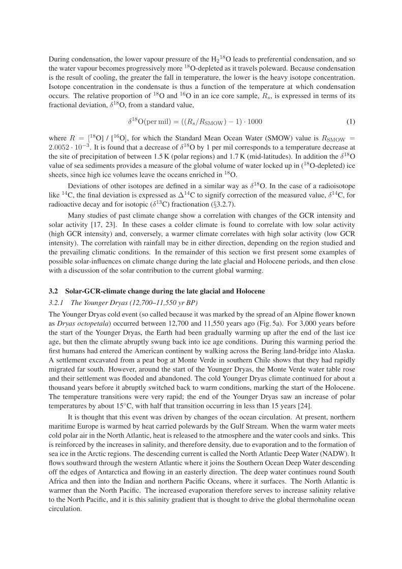
During condensation, the lower vapour pressure of the H218O leads to preferential condensation, and so

the water vapour becomes progressively more 18O-depleted as it travels poleward. Because condensationis the result of cooling, the greater the fall in temperature, the lower is the heavy isotope concentration.Isotope concentration in the condensate is thus a function of the temperature at which condensationoccurs. The relative proportion of 18O and 16O in an ice core sample, Rs, is expressed in terms of itsfractional deviation, δ18O, from a standard value,

δ18O(per mil) = ((Rs/RSMOW) − 1) · 1000 (1)

where R = [18O] / [16O], for which the Standard Mean Ocean Water (SMOW) value is RSMOW =2.0052 · 10−3. It is found that a decrease of δ18O by 1 per mil corresponds to a temperature decrease atthe site of precipitation of between 1.5 K (polar regions) and 1.7 K (mid-latitudes). In addition the δ18Ovalue of sea sediments provides a measure of the global volume of water locked up in (18O-depleted) icesheets, since high ice volumes leave the oceans enriched in 18O.

Deviations of other isotopes are defined in a similar way as δ18O. In the case of a radioisotopelike 14C, the final deviation is expressed as ∆14C to signify correction of the measured value, δ14C, forradioactive decay and for isotopic (δ13C) fractionation (§3.2.7).

Many studies of past climate change show a correlation with changes of the GCR intensity andsolar activity [17, 23]. In these cases a colder climate is found to correlate with low solar activity(high GCR intensity) and, conversely, a warmer climate correlates with high solar activity (low GCRintensity). The correlation with rainfall may be in either direction, depending on the region studied andthe prevailing climatic conditions. In the remainder of this section we first present some examples ofpossible solar-influences on climate change during the late glacial and Holocene periods, and then closewith a discussion of the solar contribution to the current global warming.

3.2 Solar-GCR-climate change during the late glacial and Holocene

3.2.1 The Younger Dryas (12,700–11,550 yr BP)

The Younger Dryas cold event (so called because it was marked by the spread of an Alpine flower knownas Dryas octopetala) occurred between 12,700 and 11,550 years ago (Fig. 5a). For 3,000 years beforethe start of the Younger Dryas, the Earth had been gradually warming up after the end of the last iceage, but then the climate abruptly swung back into ice age conditions. During this warming period thefirst humans had entered the American continent by walking across the Bering land-bridge into Alaska.A settlement excavated from a peat bog at Monte Verde in southern Chile shows that they had rapidlymigrated far south. However, around the start of the Younger Dryas, the Monte Verde water table roseand their settlement was flooded and abandoned. The cold Younger Dryas climate continued for about athousand years before it abruptly switched back to warm conditions, marking the start of the Holocene.The temperature transitions were very rapid; the end of the Younger Dryas saw an increase of polartemperatures by about 15C, with half that transition occurring in less than 15 years [24].

It is thought that this event was driven by changes of the ocean circulation. At present, northernmaritime Europe is warmed by heat carried polewards by the Gulf Stream. When the warm water meetscold polar air in the North Atlantic, heat is released to the atmosphere and the water cools and sinks. Thisis reinforced by the increases in salinity, and therefore density, due to evaporation and to the formation ofsea ice in the Arctic regions. The descending current is called the North Atlantic Deep Water (NADW). Itflows southward through the western Atlantic where it joins the Southern Ocean Deep Water descendingoff the edges of Antarctica and flowing in an easterly direction. The deep water continues round SouthAfrica and then into the Indian and northern Pacific Oceans, where it surfaces. The North Atlantic iswarmer than the North Pacific. The increased evaporation therefore serves to increase salinity relativeto the North Pacific, and it is this salinity gradient that is thought to drive the global thermohaline oceancirculation.

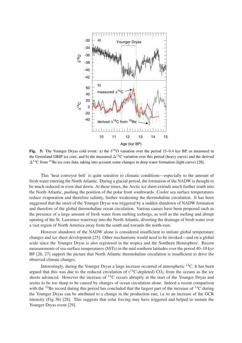
a)

b)

10 11 12 13 14 15

Age (kyr BP)

-32

-34

-36

-38

-40

-42δ18

O∆14

C

60

40

20

0

-20

-40

measured ∆14C

derived ∆14C from 10Be

Younger Dryas

Fig. 5: The Younger Dryas cold event: a) the δ18O variation over the period 15–9.4 kyr BP, as measured inthe Greenland GRIP ice core, and b) the measured ∆14C variation over this period (heavy curve) and the derived∆14C from 10Be ice core data, taking into account some changes in deep water formation (light curve) [28].

This ‘heat conveyor belt’ is quite sensitive to climatic conditions—especially to the amount offresh water entering the North Atlantic. During a glacial period, the formation of the NADW is thought tobe much reduced or even shut down. At these times, the Arctic ice sheet extends much further south intothe North Atlantic, pushing the position of the polar front southwards. Cooler sea surface temperaturesreduce evaporation and therefore salinity, further weakening the thermohaline circulation. It has beensuggested that the onset of the Younger Dryas was triggered by a sudden shutdown of NADW formationand therefore of the global thermohaline ocean circulation. Various causes have been proposed such asthe presence of a large amount of fresh water from melting icebergs, as well as the melting and abruptopening of the St. Lawrence waterway into the North Atlantic, diverting the drainage of fresh water overa vast region of North America away from the south and towards the north-east.

However shutdown of the NADW alone is considered insufficient to initiate global temperaturechanges and ice sheet development [25]. Other mechanisms would need to be invoked—and on a globalscale since the Younger Dryas is also registered in the tropics and the Southern Hemisphere. Recentmeasurements of sea-surface temperatures (SSTs) in the mid southern latitudes over the period 40–10 kyrBP [26, 27] support the picture that North Atlantic thermohaline circulation is insufficient to drive theobserved climate changes.

Interestingly, during the Younger Dryas a large increase occurred of atmospheric 14C. It has beenargued that this was due to the reduced circulation of (14C-depleted) CO2 from the oceans as the icesheets advanced. However the increase of 14C occurs abruptly at the start of the Younger Dryas andseems to be too sharp to be caused by changes of ocean circulation alone. Indeed a recent comparisonwith the 10Be record during this period has concluded that the largest part of the increase of 14C duringthe Younger Dryas can be attributed to a change in the production rate, i.e. to an increase of the GCRintensity (Fig. 5b) [28]. This suggests that solar forcing may have triggered and helped to sustain theYounger Dryas event [29].

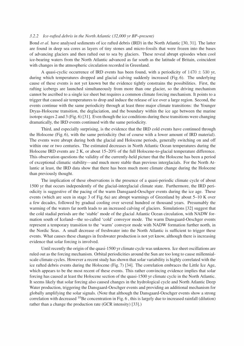
3.2.2 Ice-rafted debris in the North Atlantic (32,000 yr BP–present)

Bond et al. have analysed sediments of ice rafted debris (IRD) in the North Atlantic [30, 31]. The latterare found in deep sea cores as layers of tiny stones and micro-fossils that were frozen into the basesof advancing glaciers and then rafted out to sea by glaciers. These reveal abrupt episodes when coolice-bearing waters from the North Atlantic advanced as far south as the latitude of Britain, coincidentwith changes in the atmospheric circulation recorded in Greenland.

A quasi-cyclic occurrence of IRD events has been found, with a periodicity of 1470 ± 530 yr,during which temperatures dropped and glacial calving suddenly increased (Fig. 6). The underlyingcause of these events is not yet known but the evidence tightly constrains the possibilities. First, therafting icebergs are launched simultaneously from more than one glacier, so the driving mechanismcannot be ascribed to a single ice sheet but requires a common climate forcing mechanism. It points to atrigger that caused air temperatures to drop and induce the release of ice over a large region. Second, theevents continue with the same periodicity through at least three major climate transitions: the YoungerDryas-Holocene transition, the deglaciation, and the boundary within the ice age between the marineisotope stages 2 and 3 (Fig. 6) [31]. Even though the ice conditions during these transitions were changingdramatically, the IRD events continued with the same periodicity.

Third, and especially surprising, is the evidence that the IRD cold events have continued throughthe Holocene (Fig. 6), with the same periodicity (but of course with a lower amount of IRD material).The events were abrupt during both the glacial and Holocene periods, generally switching on and offwithin one or two centuries. The estimated decreases in North Atlantic Ocean temperatures during theHolocene IRD events are 2 K, or about 15–20% of the full Holocene-to-glacial temperature difference.This observation questions the validity of the currently-held picture that the Holocene has been a periodof exceptional climatic stability—and much more stable than previous interglacials. For the North At-lantic at least, the IRD data show that there has been much more climate change during the Holocenethan previously thought.

The implication of these observations is the presence of a quasi-periodic climate cycle of about1500 yr that occurs independently of the glacial-interglacial climate state. Furthermore, the IRD peri-odicity is suggestive of the pacing of the warm Dansgaard-Oeschger events during the ice age. Theseevents (which are seen in stage 3 of Fig. 6a) are abrupt warmings of Greenland by about 5–10 K overa few decades, followed by gradual cooling over several hundred or thousand years. Presumably thewarming of the waters far north leads to an increased calving of glaciers. Simulations [32] suggest thatthe cold stadial periods are the ‘stable’ mode of the glacial Atlantic Ocean circulation, with NADW for-mation south of Iceland—the so-called ‘cold’ conveyor mode. The warm Dansgaard-Oeschger eventsrepresent a temporary transition to the ‘warm’ conveyor mode with NADW formation further north, inthe Nordic Seas. A small decrease of freshwater into the North Atlantic is sufficient to trigger theseevents. What causes these changes in freshwater production is not yet know, although there is increasingevidence that solar forcing is involved.

Until recently the origin of the quasi-1500 yr climate cycle was unknown. Ice sheet oscillations areruled out as the forcing mechanism. Orbital periodicities around the Sun are too long to cause millennial-scale climate cycles. However a recent study has shown that solar variability is highly correlated with theice rafted debris events during the Holocene (Fig. 7) [34]. The correlation embraces the Little Ice Age,which appears to be the most recent of these events. This rather convincing evidence implies that solarforcing has caused at least the Holocene section of the quasi-1500 yr climate cycle in the North Atlantic.It seems likely that solar forcing also caused changes in the hydrological cycle and North Atlantic DeepWater production, triggering the Dansgaard-Oeschger events and providing an additional mechanism forglobally amplifying the solar signals. (Note that although the Dansgaard-Oeschger events show a strongcorrelation with decreased 10Be concentration in Fig. 6 , this is largely due to increased rainfall (dilution)rather than a change the production rate (GCR intensity) [33].)

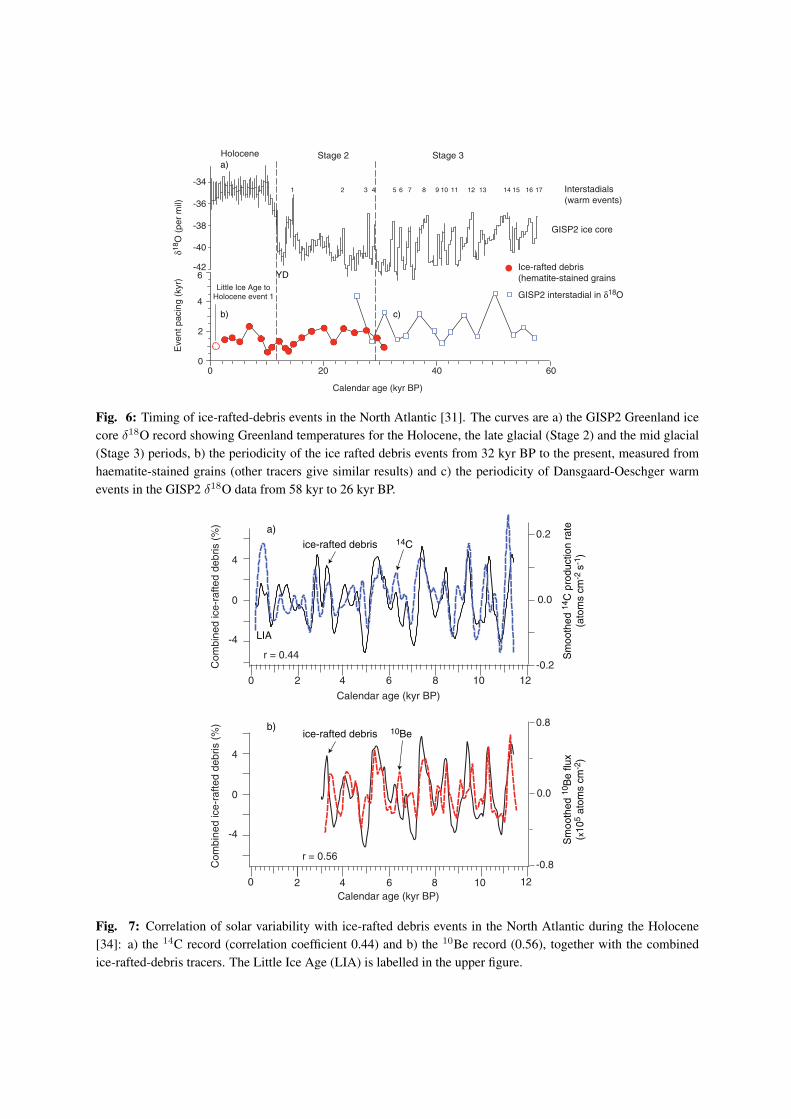
6040200

4

2

0

GISP2 interstadial in δ18O

Ice-rafted debris(hematite-stained grains

Little Ice Age toHolocene event 1

Calendar age (kyr BP)

6

1 3 5 8 9 172 6 13 1615141210 11

-42

-40

-38

-36

-34Interstadials(warm events)

Holocene Stage 2 Stage 3

GISP2 ice core

δ18O

(pe

r m

il)E

vent

pac

ing

(kyr

)74

YD

a)

b) c)

Fig. 6: Timing of ice-rafted-debris events in the North Atlantic [31]. The curves are a) the GISP2 Greenland icecore δ18O record showing Greenland temperatures for the Holocene, the late glacial (Stage 2) and the mid glacial(Stage 3) periods, b) the periodicity of the ice rafted debris events from 32 kyr BP to the present, measured fromhaematite-stained grains (other tracers give similar results) and c) the periodicity of Dansgaard-Oeschger warmevents in the GISP2 δ18O data from 58 kyr to 26 kyr BP.

12108642

r = 0.56

Calendar age (kyr BP)

-4

0

4

-4

0

4

-0.8

0.0

0.8

Com

bine

d ic

e-ra

fted

debr

is (

%)

Com

bine

d ic

e-ra

fted

debr

is (

%)

r = 0.44

121086420

0.2

0.0

-0.2

Calendar age (kyr BP)

ice-rafted debris

14C

10Be

Sm

ooth

ed 1

0 Be

flux

( x10

5 at

oms

cm-2

)S

moo

thed

14 C

pro

duct

ion

rate

(ato

ms

cm-2

s-1

)

ice-rafted debris

0

a)

b)

LIA

Fig. 7: Correlation of solar variability with ice-rafted debris events in the North Atlantic during the Holocene[34]: a) the 14C record (correlation coefficient 0.44) and b) the 10Be record (0.56), together with the combinedice-rafted-debris tracers. The Little Ice Age (LIA) is labelled in the upper figure.

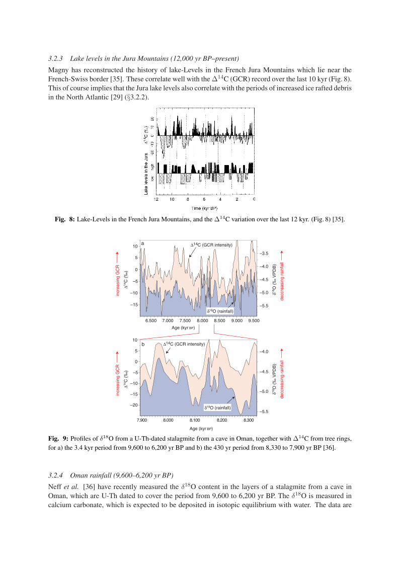
3.2.3 Lake levels in the Jura Mountains (12,000 yr BP–present)

Magny has reconstructed the history of lake-Levels in the French Jura Mountains which lie near theFrench-Swiss border [35]. These correlate well with the ∆14C (GCR) record over the last 10 kyr (Fig. 8).This of course implies that the Jura lake levels also correlate with the periods of increased ice rafted debrisin the North Atlantic [29] (§3.2.2).

Fig. 8: Lake-Levels in the French Jura Mountains, and the ∆14C variation over the last 12 kyr. (Fig. 8) [35].

6.500 7.000 7.500 8.000 8.500 9.000 9.500

–15

–10

–5

0

5

10

∆14C

(‰

)

δ18O

(‰

VP

DB

)

Age (kyr BP)

8.0007.900 8.100 8.200 8.300

Age (kyr BP)

a

–5.5

–5.0

–4.5

–4.0

–3.5

–5.5

–5.0

–4.5

–4.0

δ18O (rainfall)

∆14C (GCR intensity)

–20

–15

–10

–5

0

5

10b ∆14C (GCR intensity)

decc

reas

ing

rain

fall

decc

reas

ing

rain

fall

incr

easi

ng G

CR

∆14C

(‰

)

δ18O

(‰

VP

DB

)

incr

easi

ng G

CR

δ18O (rainfall)

Fig. 9: Profiles of δ18O from a U-Th-dated stalagmite from a cave in Oman, together with ∆14C from tree rings,for a) the 3.4 kyr period from 9,600 to 6,200 yr BP and b) the 430 yr period from 8,330 to 7,900 yr BP [36].

3.2.4 Oman rainfall (9,600–6,200 yr BP)

Neff et al. [36] have recently measured the δ18O content in the layers of a stalagmite from a cave inOman, which are U-Th dated to cover the period from 9,600 to 6,200 yr BP. The δ18O is measured incalcium carbonate, which is expected to be deposited in isotopic equilibrium with water. The data are

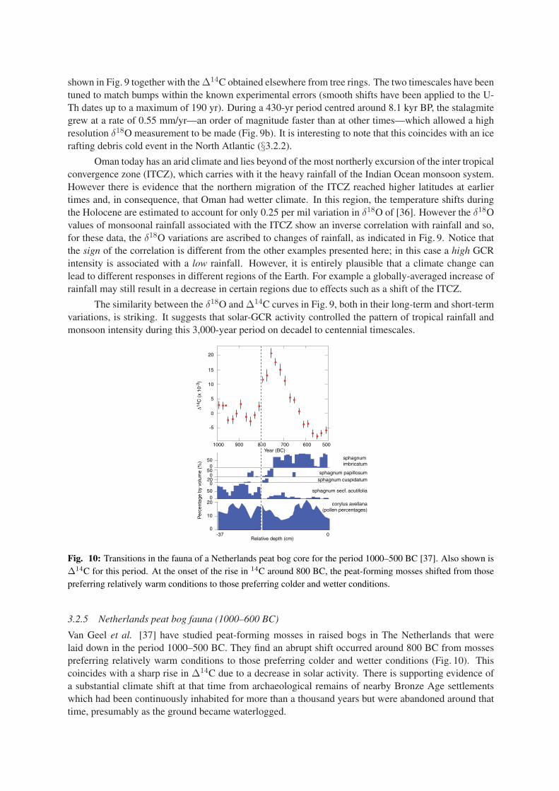
shown in Fig. 9 together with the ∆14C obtained elsewhere from tree rings. The two timescales have beentuned to match bumps within the known experimental errors (smooth shifts have been applied to the U-Th dates up to a maximum of 190 yr). During a 430-yr period centred around 8.1 kyr BP, the stalagmitegrew at a rate of 0.55 mm/yr—an order of magnitude faster than at other times—which allowed a highresolution δ18O measurement to be made (Fig. 9b). It is interesting to note that this coincides with an icerafting debris cold event in the North Atlantic (§3.2.2).

Oman today has an arid climate and lies beyond of the most northerly excursion of the inter tropicalconvergence zone (ITCZ), which carries with it the heavy rainfall of the Indian Ocean monsoon system.However there is evidence that the northern migration of the ITCZ reached higher latitudes at earliertimes and, in consequence, that Oman had wetter climate. In this region, the temperature shifts duringthe Holocene are estimated to account for only 0.25 per mil variation in δ18O of [36]. However the δ18Ovalues of monsoonal rainfall associated with the ITCZ show an inverse correlation with rainfall and so,for these data, the δ18O variations are ascribed to changes of rainfall, as indicated in Fig. 9. Notice thatthe sign of the correlation is different from the other examples presented here; in this case a high GCRintensity is associated with a low rainfall. However, it is entirely plausible that a climate change canlead to different responses in different regions of the Earth. For example a globally-averaged increase ofrainfall may still result in a decrease in certain regions due to effects such as a shift of the ITCZ.

The similarity between the δ18O and ∆14C curves in Fig. 9, both in their long-term and short-termvariations, is striking. It suggests that solar-GCR activity controlled the pattern of tropical rainfall andmonsoon intensity during this 3,000-year period on decadel to centennial timescales.

∆14 C

(x

10-3

)P

erce

ntag

e by

vol

ume

(%)

20

15

10

5

0

-5

500

500

200

500

20

10

0

1000 900 800 700 600 500Year (BC)

-37 0Relative depth (cm)

sphagnumimbricatum

sphagnum papillosumsphagnum cuspidatum

sphagnum secf. acutifolia

corylus avellana(pollen percentages)

Fig. 10: Transitions in the fauna of a Netherlands peat bog core for the period 1000–500 BC [37]. Also shown is∆14C for this period. At the onset of the rise in 14C around 800 BC, the peat-forming mosses shifted from thosepreferring relatively warm conditions to those preferring colder and wetter conditions.

3.2.5 Netherlands peat bog fauna (1000–600 BC)

Van Geel et al. [37] have studied peat-forming mosses in raised bogs in The Netherlands that werelaid down in the period 1000–500 BC. They find an abrupt shift occurred around 800 BC from mossespreferring relatively warm conditions to those preferring colder and wetter conditions (Fig. 10). Thiscoincides with a sharp rise in ∆14C due to a decrease in solar activity. There is supporting evidence ofa substantial climate shift at that time from archaeological remains of nearby Bronze Age settlementswhich had been continuously inhabited for more than a thousand years but were abandoned around thattime, presumably as the ground became waterlogged.

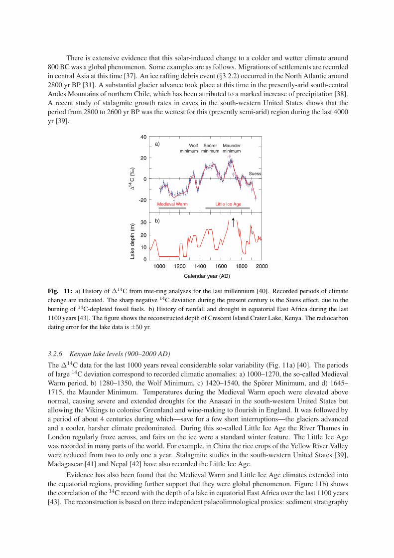
There is extensive evidence that this solar-induced change to a colder and wetter climate around800 BC was a global phenomenon. Some examples are as follows. Migrations of settlements are recordedin central Asia at this time [37]. An ice rafting debris event (§3.2.2) occurred in the North Atlantic around2800 yr BP [31]. A substantial glacier advance took place at this time in the presently-arid south-centralAndes Mountains of northern Chile, which has been attributed to a marked increase of precipitation [38].A recent study of stalagmite growth rates in caves in the south-western United States shows that theperiod from 2800 to 2600 yr BP was the wettest for this (presently semi-arid) region during the last 4000yr [39].

40

20

0

-20

Maunderminimum

Spörerminimum

Wolfminimum

Suess

a)

b)

∆14C

(‰

)

1000 1200 1400 1600 1800 20000

10

20

30

Calendar year (AD)

Lake

dep

th (

m)

Little Ice AgeMedieval Warm

Fig. 11: a) History of ∆14C from tree-ring analyses for the last millennium [40]. Recorded periods of climatechange are indicated. The sharp negative 14C deviation during the present century is the Suess effect, due to theburning of 14C-depleted fossil fuels. b) History of rainfall and drought in equatorial East Africa during the last1100 years [43]. The figure shows the reconstructed depth of Crescent Island Crater Lake, Kenya. The radiocarbondating error for the lake data is ±50 yr.

3.2.6 Kenyan lake levels (900–2000 AD)

The ∆14C data for the last 1000 years reveal considerable solar variability (Fig. 11a) [40]. The periodsof large 14C deviation correspond to recorded climatic anomalies: a) 1000–1270, the so-called MedievalWarm period, b) 1280–1350, the Wolf Minimum, c) 1420–1540, the Sporer Minimum, and d) 1645–1715, the Maunder Minimum. Temperatures during the Medieval Warm epoch were elevated abovenormal, causing severe and extended droughts for the Anasazi in the south-western United States butallowing the Vikings to colonise Greenland and wine-making to flourish in England. It was followed bya period of about 4 centuries during which—save for a few short interruptions—the glaciers advancedand a cooler, harsher climate predominated. During this so-called Little Ice Age the River Thames inLondon regularly froze across, and fairs on the ice were a standard winter feature. The Little Ice Agewas recorded in many parts of the world. For example, in China the rice crops of the Yellow River Valleywere reduced from two to only one a year. Stalagmite studies in the south-western United States [39],Madagascar [41] and Nepal [42] have also recorded the Little Ice Age.

Evidence has also been found that the Medieval Warm and Little Ice Age climates extended intothe equatorial regions, providing further support that they were global phenomenon. Figure 11b) showsthe correlation of the 14C record with the depth of a lake in equatorial East Africa over the last 1100 years[43]. The reconstruction is based on three independent palaeolimnological proxies: sediment stratigraphy

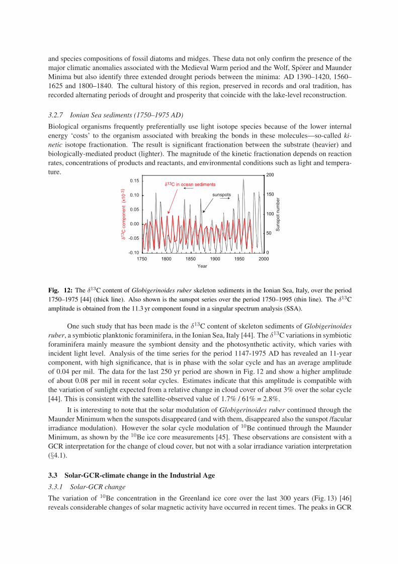
and species compositions of fossil diatoms and midges. These data not only confirm the presence of themajor climatic anomalies associated with the Medieval Warm period and the Wolf, Sporer and MaunderMinima but also identify three extended drought periods between the minima: AD 1390–1420, 1560–1625 and 1800–1840. The cultural history of this region, preserved in records and oral tradition, hasrecorded alternating periods of drought and prosperity that coincide with the lake-level reconstruction.

3.2.7 Ionian Sea sediments (1750–1975 AD)

Biological organisms frequently preferentially use light isotope species because of the lower internalenergy ‘costs’ to the organism associated with breaking the bonds in these molecules—so-called ki-netic isotope fractionation. The result is significant fractionation between the substrate (heavier) andbiologically-mediated product (lighter). The magnitude of the kinetic fractionation depends on reactionrates, concentrations of products and reactants, and environmental conditions such as light and tempera-ture.

δ13C in ocean sediments

1750 1800 1850 1900 1950 2000

0

50

100

150

200

sunspots

Sun

spot

num

ber

Year

δ13C

com

ponent

(x10

-3)

0.15

0.10

0.05

0.00

-0.05

-0.10

Fig. 12: The δ13C content of Globigerinoides ruber skeleton sediments in the Ionian Sea, Italy, over the period1750–1975 [44] (thick line). Also shown is the sunspot series over the period 1750–1995 (thin line). The δ13Camplitude is obtained from the 11.3 yr component found in a singular spectrum analysis (SSA).

One such study that has been made is the δ13C content of skeleton sediments of Globigerinoidesruber, a symbiotic planktonic foraminifera, in the Ionian Sea, Italy [44]. The δ13C variations in symbioticforaminifera mainly measure the symbiont density and the photosynthetic activity, which varies withincident light level. Analysis of the time series for the period 1147-1975 AD has revealed an 11-yearcomponent, with high significance, that is in phase with the solar cycle and has an average amplitudeof 0.04 per mil. The data for the last 250 yr period are shown in Fig. 12 and show a higher amplitudeof about 0.08 per mil in recent solar cycles. Estimates indicate that this amplitude is compatible withthe variation of sunlight expected from a relative change in cloud cover of about 3% over the solar cycle[44]. This is consistent with the satellite-observed value of 1.7% / 61% = 2.8%.

It is interesting to note that the solar modulation of Globigerinoides ruber continued through theMaunder Minimum when the sunspots disappeared (and with them, disappeared also the sunspot /facularirradiance modulation). However the solar cycle modulation of 10Be continued through the MaunderMinimum, as shown by the 10Be ice core measurements [45]. These observations are consistent with aGCR interpretation for the change of cloud cover, but not with a solar irradiance variation interpretation(§4.1).

3.3 Solar-GCR-climate change in the Industrial Age

3.3.1 Solar-GCR change

The variation of 10Be concentration in the Greenland ice core over the last 300 years (Fig. 13) [46]reveals considerable changes of solar magnetic activity have occurred in recent times. The peaks in GCR

1700 1750 1800 1850

Year

1900 1950 2000

10B

e co

ncen

trat

ion

(x 1

04 a

tom

s/g)

Daltonminimum

10Be concentration

Maunder minimum

0.4

0.6

0

0.2

0.8

1.0

1.2

1.4

1.6

Solar open magnetic flux

Sol

ar m

agne

tic fl

ux (

x 10

14 W

b)

0

5

10

15

Fig. 13: Variation of 10Be concentration in the Greenland ice core over the last 300 years [46], due to changesof solar magnetic activity (thin line). The variation of the solar coronal source flux, FS , over the last 140 years isshown by the thick line [11] (note inverted scale and unsupressed zero). In the period since 1901, the increase ofthe solar open magnetic flux has been a factor 2.3.

intensity over this period coincide with the cold spells of the Maunder Minimum and Dalton Minimum.

More recently, during the 20th century, the 10Be data show a substantial reduction of the GCRintensity due to a marked increase in the strength of the solar wind. The latter is independently confirmedby the <aa> geomagnetic index,6 for which there is a continuous record extending back to 1868 andcovering 12 sunspot cycles. From the level of geomagnetic activity seen at Earth in the <aa> index,Lockwood et al. [11] have estimated the source magnetic flux, Fs, that leaves the corona and enters theheliosphere. Their method to derive the coronal source flux has been successfully tested against near-Earth interplanetary space measurements made since 1963, during which time the coronal source fluxhas been observed to rise a factor 1.4. In the period since 1901, the calculated increase has been a factor2.3 (indicated by the thick line in Fig. 13).

The open solar flux shows a highly significant anti-correlation with the GCR intensity and so canbe reliably used to reconstruct the global GCR intensity over the last 140 years [47]. The data are shownin Fig. 14 (left-hand axis) and indicate a reduction of GCR intensity during the last century by about 20%for the Climax neutron monitors (3 GeV/c cutoff). This implies global average reductions of about 15%at the top of the troposphere, or about 10% at 3 km altitude (§4.3).

Assuming for the moment the existence of a linear relationship between GCR intensity and thelow cloud absolute fraction (Fig. 2), then the open solar magnetic flux can also be used to reconstruct thechange in low cloud fraction over the same period. The result is shown in Fig. 14 (right-hand axis) [16]and indicates a reduction of low cloud fraction since 1900 by about 1.3% absolute (4.6% relative). Sincelow clouds are estimated to contribute a net radiative forcing of -17 Wm−2 (Table 1), this corresponds toa forcing of about 0.046×17 = +0.8 Wm−2, which is climatically significant (§3.3.5). Overall, these datasuggest that a 10% reduction of GCR flux at 3 km altitude is associated with a 4.6% relative reduction oflow cloud cover. This would imply a rather high sensitivity of low clouds to GCR intensity, if we assumethey are linked.

6The <aa> geomagnetic index is a sensitive measurement by two antipodal stations of short-term (3-hour interval) vari-ations of the geomagnetic field at the Earth’s surface, which is affected by the interactions of the solar wind with the Earth’smagnetosphere.

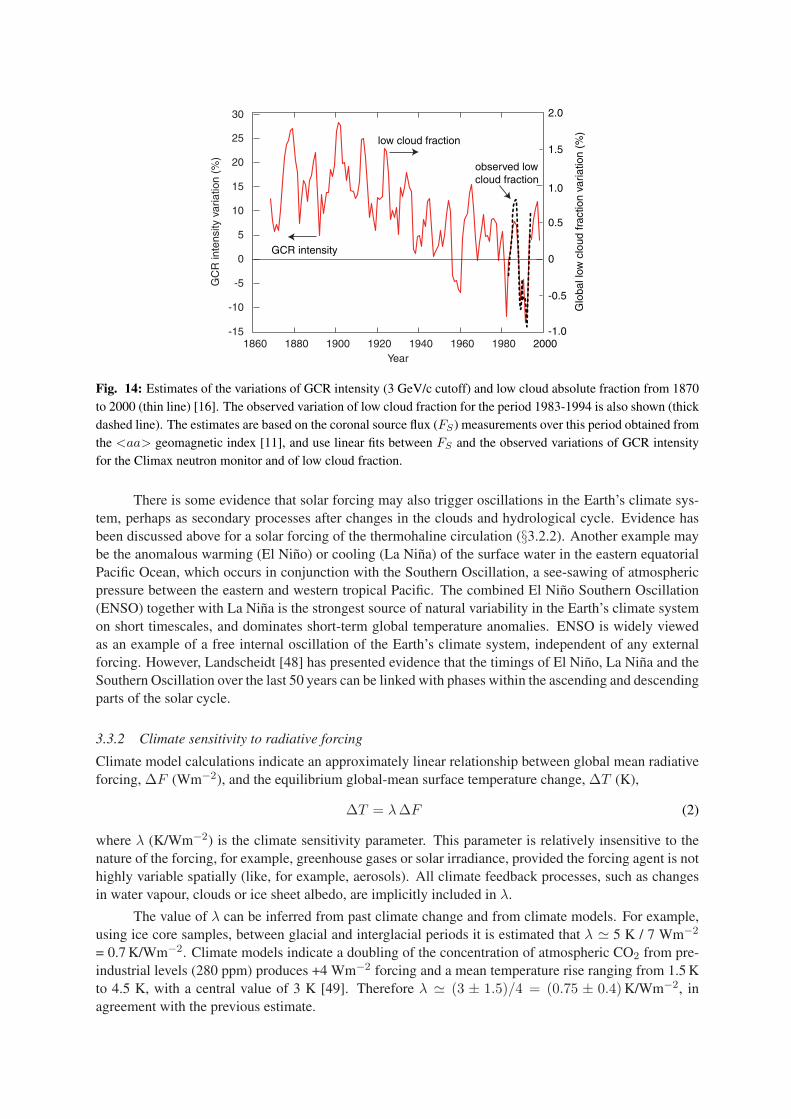
1860

GC

R in

tens

ity v

aria

tion

(%)

-10

-15

-5

10

15

20

25

30

0

5

1880 1900 1920 1940 1960 1980 2000 Year

0

0.5

1.5

-0.5

1.0

-1.0

2.0

Glo

bal l

ow c

loud

frac

tion

varia

tion

(%)

GCR intensity

low cloud fraction

observed lowcloud fraction

Fig. 14: Estimates of the variations of GCR intensity (3 GeV/c cutoff) and low cloud absolute fraction from 1870to 2000 (thin line) [16]. The observed variation of low cloud fraction for the period 1983-1994 is also shown (thickdashed line). The estimates are based on the coronal source flux (FS) measurements over this period obtained fromthe <aa> geomagnetic index [11], and use linear fits between FS and the observed variations of GCR intensityfor the Climax neutron monitor and of low cloud fraction.

There is some evidence that solar forcing may also trigger oscillations in the Earth’s climate sys-tem, perhaps as secondary processes after changes in the clouds and hydrological cycle. Evidence hasbeen discussed above for a solar forcing of the thermohaline circulation (§3.2.2). Another example maybe the anomalous warming (El Nino) or cooling (La Nina) of the surface water in the eastern equatorialPacific Ocean, which occurs in conjunction with the Southern Oscillation, a see-sawing of atmosphericpressure between the eastern and western tropical Pacific. The combined El Nino Southern Oscillation(ENSO) together with La Nina is the strongest source of natural variability in the Earth’s climate systemon short timescales, and dominates short-term global temperature anomalies. ENSO is widely viewedas an example of a free internal oscillation of the Earth’s climate system, independent of any externalforcing. However, Landscheidt [48] has presented evidence that the timings of El Nino, La Nina and theSouthern Oscillation over the last 50 years can be linked with phases within the ascending and descendingparts of the solar cycle.

3.3.2 Climate sensitivity to radiative forcing

Climate model calculations indicate an approximately linear relationship between global mean radiativeforcing, ∆F (Wm−2), and the equilibrium global-mean surface temperature change, ∆T (K),

∆T = λ ∆F (2)

where λ (K/Wm−2) is the climate sensitivity parameter. This parameter is relatively insensitive to thenature of the forcing, for example, greenhouse gases or solar irradiance, provided the forcing agent is nothighly variable spatially (like, for example, aerosols). All climate feedback processes, such as changesin water vapour, clouds or ice sheet albedo, are implicitly included in λ.

The value of λ can be inferred from past climate change and from climate models. For example,using ice core samples, between glacial and interglacial periods it is estimated that λ 5 K / 7 Wm−2

= 0.7 K/Wm−2. Climate models indicate a doubling of the concentration of atmospheric CO2 from pre-industrial levels (280 ppm) produces +4 Wm−2 forcing and a mean temperature rise ranging from 1.5 Kto 4.5 K, with a central value of 3 K [49]. Therefore λ (3 ± 1.5)/4 = (0.75 ± 0.4) K/Wm−2, inagreement with the previous estimate.

These figures can be compared with the response of the Earth if it were to act as a simple blackbody. In this case the radiant emittance is R = σT 4, where σ is the Stefan-Boltzmann constant. The radi-ation from a black body varies as ∆R/R = 4∆T/T , so that ∆T = (T/4R) ∆R. Since ∆R/R = ∆I/I ,the fractional change in solar irradiance, it follows that λ0 = T/4I . The effective radiating temperatureof the Earth is T 266 K, and the global mean solar irradiance reaching the lower troposphere isI 0.7 × 1366/4 240 Wm−2 (the factor 0.7 accounts for shortwave albedo and the factor 4 aver-ages the solar irradiance of 1366 Wm−2 over the full surface area of the Earth). We thereby estimateλ0 = 266/(4 · 240) 0.3 K/Wm−2 for the Earth in the absence of any feedbacks. Therefore the climatefeedback factor of the Earth is between a factor of about 1.2 and 4, with a central value of 2.5, and itis greater than one, amplifying the temperature response to a radiative forcing compared with that for asimple black body.

3.3.3 Solar contribution to the current global warming

The reconstructed global mean surface temperature of the Earth between 1860 and 2001 (Fig. 15) [49]indicates a warming of about 0.6 K over this period. A notable feature of the warming is that it didnot rise smoothly along with the steadily increasing emissions of anthropogenic greenhouse gases butseemed to flatten, or even reverse sign, during the period 1945–1980.

1860 1880 1900 1920 1940 1960 1980 2000Year

Data from thermometers

0.8

0.4

0.0

0.4

0.8

Tem

pera

ture

diff

eren

ce (

0 C)

rela

tive

to 1

961-

1990

ave

rage

GLOBAL AVERAGE

Fig. 15: The global mean surface temperature of the Earth, 1860–2001, relative to the 1961–1990 average [49].

A component of this temperature reconstruction is sea-surface temperatures (SSTs), which havebeen measured on a routine basis by ocean-going ships since the mid-19th century. The SST record is aparticularly valuable measure of global climate since it represents over 70% of the Earth’s surface andis much more spatially and temporally homogeneous than the land surface, as well as being free of suchproblems as the warming from ‘urban heat islands’. The mean SSTs over the period 1860–1985, for theAtlantic, Pacific and Indian Oceans, are shown in Fig. 16, together with the global mean SST [50]. Allof these oceans show a temperature rise that levels off in the same period around 1945–1980, as wellas a cooling around the beginning of the last century. Both of these features are characteristic of solaractivity, as can be seen in the smoothed sunspot number (Fig. 16) and in the GCR intensity (Fig. 17).

A world-wide simultaneous variation of SST puts severe constraints on a possible forcing mech-anism. Since the same characteristic features are seen in all oceans, they are unlikely to be caused bychanges such as El Nino events, shifts in wind patterns or changes in the thermohaline circulation, whichwould lead to differences between the oceans. The mechanism could in principle be increases of anthro-pogenic greenhouse gases, but the variation in the first half of the 20th century occurred before thesewere significant. There were insufficient volcanic events to account for the mid-century cooling. Theinescapable conclusion is that these data provide quite strong evidence that solar variability was the pri-

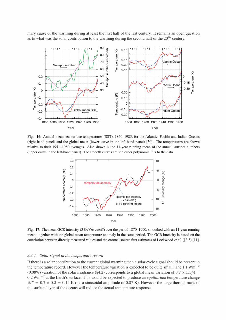
mary cause of the warming during at least the first half of the last century. It remains an open questionas to what was the solar contribution to the warming during the second half of the 20th century.

-0.4

-0.3

-0.2

-0.1

0

0.1

0.2

Tem

pera

ture

(K

)

Tem

pera

ture

(K

)T

empe

ratu

re (

K)

Tem

pera

ture

(K

)

0

-0.30

-0.15

0.15

0.30-0.30

-0.15

0

-0.45

-0.30

-0.15

0

0.15

Atlantic Ocean

Pacific Ocean

Indian Ocean

Sunspot number

Global mean SST

1980196019401920190018801860

90

80

70

60

50

40

30

Sun

spot

num

ber

(sm

ooth

ed)

Year

1980196019401920190018801860

Year

Fig. 16: Annual mean sea-surface temperatures (SST), 1860–1985, for the Atlantic, Pacific and Indian Oceans(right-hand panel) and the global mean (lower curve in the left-hand panel) [50]. The temperatures are shownrelative to their 1951–1980 averages. Also shown is the 11-year running mean of the annual sunspot numbers(upper curve in the left-hand panel). The smooth curves are 7th order polynomial fits to the data.

1860 1880 1900 1920 1940 1960 1980 2000

0

-5

-10

5

10

15-0.4

-0.3

-0.2

-0.1

0

0.1

0.2

0.3

Year

cosmic ray intensity(> 3 GeV/c)

(11-y running mean)

temperature anomaly

Tem

pera

ture

ano

mal

y (o

C)

GC

R in

tens

ity c

hang

e (%

)

Fig. 17: The mean GCR intensity (3 GeV/c cutoff) over the period 1870–1990, smoothed with an 11-year runningmean, together with the global mean temperature anomaly in the same period. The GCR intensity is based on thecorrelation between directly measured values and the coronal source flux estimates of Lockwood et al. (§3.3) [11].

3.3.4 Solar signal in the temperature record

If there is a solar contribution to the current global warming then a solar cycle signal should be present inthe temperature record. However the temperature variation is expected to be quite small. The 1.1 Wm−2

(0.08%) variation of the solar irradiance (§4.2) corresponds to a global mean variation of 0.7 × 1.1/4 =0.2 Wm−2 at the Earth’s surface. This would be expected to produce an equilibrium temperature change∆T = 0.7 × 0.2 = 0.14 K (i.e. a sinusoidal amplitude of 0.07 K). However the large thermal mass ofthe surface layer of the oceans will reduce the actual temperature response.

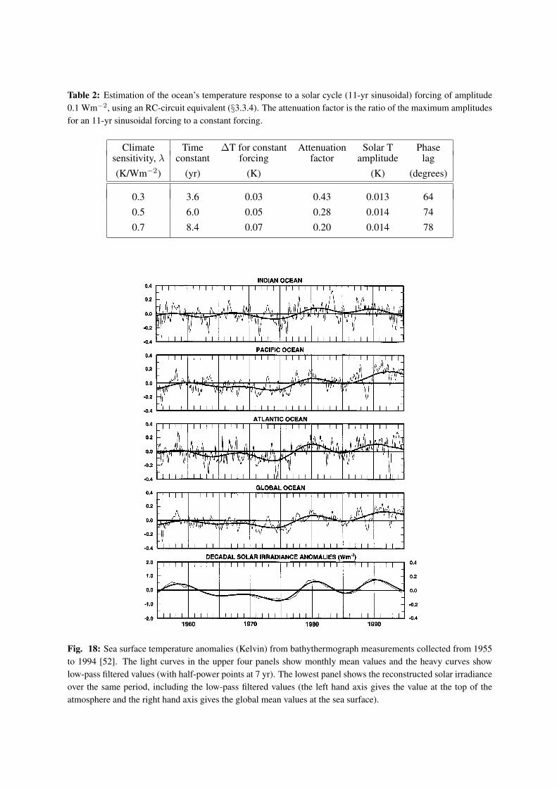
Table 2: Estimation of the ocean’s temperature response to a solar cycle (11-yr sinusoidal) forcing of amplitude0.1 Wm−2, using an RC-circuit equivalent (§3.3.4). The attenuation factor is the ratio of the maximum amplitudesfor an 11-yr sinusoidal forcing to a constant forcing.

Climate Time ∆T for constant Attenuation Solar T Phasesensitivity, λ constant forcing factor amplitude lag

(K/Wm−2) (yr) (K) (K) (degrees)

0.3 3.6 0.03 0.43 0.013 64

0.5 6.0 0.05 0.28 0.014 74

0.7 8.4 0.07 0.20 0.014 78

Fig. 18: Sea surface temperature anomalies (Kelvin) from bathythermograph measurements collected from 1955to 1994 [52]. The light curves in the upper four panels show monthly mean values and the heavy curves showlow-pass filtered values (with half-power points at 7 yr). The lowest panel shows the reconstructed solar irradianceover the same period, including the low-pass filtered values (the left hand axis gives the value at the top of theatmosphere and the right hand axis gives the global mean values at the sea surface).

We can estimate the damping effect of the oceans by considering an analogous electromagneticRC-circuit equivalent for the ocean surface layer: a resistor and capacitor in series, which are set intoforced oscillation by a sinusoidal voltage [51]. In this analogy, forcing heat fluxes are analogous tocurrent, temperature to voltage, the ocean to a capacitor and the climate sensitivity parameter to a resistor.The value of the capacitor can be estimated by assuming the ocean can be represented by a well-mixedupper layer of about 90 m depth that is effectively isolated from thermal exchange with deeper water,except by relatively slow diffusion. Table 2 summarises the expected ocean response to a solar cycle(11-yr sinusoidal) forcing of amplitude 0.1 Wm−2. The estimated solar cycle temperature amplitude is0.014 K, with a phase lag of about 65–80 degrees. The temperature response is essentially independentof the climate sensitivity, λ, since the larger constant-forcing temperatures at higher λ are compensatedby longer time constants and therefore larger attenuation factors for the short solar cycle. The attenuationfactors are large, e.g. a factor 5 for λ = 0.7 K/Wm−2, corresponding to an 8.4 yr time constant.

White et al. [52, 53] have analysed the SST data for the period 1900–1991 and the bathyther-mograph data for 1955–1996. Their analyses reveal convincing solar signals in the Indian, Pacific andAtlantic Oceans which all show comparable amplitudes and phases (Fig. 18). The solar cycle amplitudeis (0.03±0.005) K and it lags the changes in solar irradiance by about 0–65. This amplitude is twice theexpected value (Table 2). An inter-decadel (18–25 yr) solar signal is also observed with (0.04±0.005) Kamplitude and 15–50 phase lag, which is consistent with the expected value from estimated longer-termchanges in solar irradiance [53]. In summary, there is indeed clear evidence of a solar signal in the tem-perature record but the 11-yr oscillation appears to be about a factor two larger than expected, suggestingeither an error in the modelling, or else the presence of a mechanism that amplifies the solar forcing.

Rad

iativ

e fo

rcin

g (W

/m2 )

greenhouse gases aerosols & clouds

natural

CH4 N20CO2 CFC O3

cloudalbedo

cloudlifetime

solardirect

solarindirect

landalbedo

aerosoldirect

aerosol indirect

volcanicaerosol

(range of10y mean)

trop.

strat.

+2

+1

0

-1

-2

anthropogenic natural

land use

total +2.9 W/m2 +0.8 W/m2

?+0.4 W/m2

(solar)-0.2 -1.4 (-2.4) W/m2

GCR-cloud?Sun & volcanoes

a) b)

?

Fig. 19: a) The global mean radiative forcings of the climate for the period from pre-industrial (1750) to present,as estimated by the Intergovernmental Panel on Climate Change (IPCC) [49]. A positive forcing causes a globalmean warming, and a negative forcing causes a cooling. The aerosol indirect contributions are poorly known,especially the second one (changes of cloud lifetime), and have large uncertainties. b) Estimated radiative forcingdue to the putative solar indirect effect if GCRs and low cloud cover are causally linked.

3.3.5 Radiative forcings

The global mean radiative forcings of the climate in the Industrial Age, as estimated by the Intergov-ernmental Panel on Climate Change (IPCC), are shown in Fig. 19a) [49]. Whereas the forcings duegreenhouse gases are known quite well, there are large uncertainties associated with the forcings dueto anthropogenic aerosols. The latter are separated into aerosol direct effects (albedo and absorption ofsolar radiation) and aerosol indirect effects due to their influence on clouds (the so-called first indirect

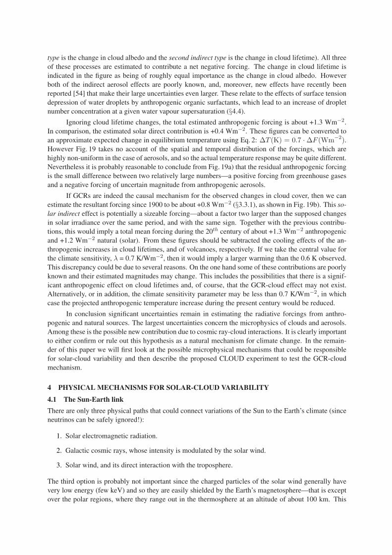
type is the change in cloud albedo and the second indirect type is the change in cloud lifetime). All threeof these processes are estimated to contribute a net negative forcing. The change in cloud lifetime isindicated in the figure as being of roughly equal importance as the change in cloud albedo. Howeverboth of the indirect aerosol effects are poorly known, and, moreover, new effects have recently beenreported [54] that make their large uncertainties even larger. These relate to the effects of surface tensiondepression of water droplets by anthropogenic organic surfactants, which lead to an increase of dropletnumber concentration at a given water vapour supersaturation (§4.4).

Ignoring cloud lifetime changes, the total estimated anthropogenic forcing is about +1.3 Wm−2.In comparison, the estimated solar direct contribution is +0.4 Wm−2. These figures can be converted toan approximate expected change in equilibrium temperature using Eq. 2: ∆T (K) = 0.7 · ∆F (Wm−2).However Fig. 19 takes no account of the spatial and temporal distribution of the forcings, which arehighly non-uniform in the case of aerosols, and so the actual temperature response may be quite different.Nevertheless it is probably reasonable to conclude from Fig. 19a) that the residual anthropogenic forcingis the small difference between two relatively large numbers—a positive forcing from greenhouse gasesand a negative forcing of uncertain magnitude from anthropogenic aerosols.

If GCRs are indeed the causal mechanism for the observed changes in cloud cover, then we canestimate the resultant forcing since 1900 to be about +0.8 Wm−2 (§3.3.1), as shown in Fig. 19b). This so-lar indirect effect is potentially a sizeable forcing—about a factor two larger than the supposed changesin solar irradiance over the same period, and with the same sign. Together with the previous contribu-tions, this would imply a total mean forcing during the 20th century of about +1.3 Wm−2 anthropogenicand +1.2 Wm−2 natural (solar). From these figures should be subtracted the cooling effects of the an-thropogenic increases in cloud lifetimes, and of volcanoes, respectively. If we take the central value forthe climate sensitivity, λ = 0.7 K/Wm−2, then it would imply a larger warming than the 0.6 K observed.This discrepancy could be due to several reasons. On the one hand some of these contributions are poorlyknown and their estimated magnitudes may change. This includes the possibilities that there is a signif-icant anthropogenic effect on cloud lifetimes and, of course, that the GCR-cloud effect may not exist.Alternatively, or in addition, the climate sensitivity parameter may be less than 0.7 K/Wm−2, in whichcase the projected anthropogenic temperature increase during the present century would be reduced.

In conclusion significant uncertainties remain in estimating the radiative forcings from anthro-pogenic and natural sources. The largest uncertainties concern the microphysics of clouds and aerosols.Among these is the possible new contribution due to cosmic ray-cloud interactions. It is clearly importantto either confirm or rule out this hypothesis as a natural mechanism for climate change. In the remain-der of this paper we will first look at the possible microphysical mechanisms that could be responsiblefor solar-cloud variability and then describe the proposed CLOUD experiment to test the GCR-cloudmechanism.

4 PHYSICAL MECHANISMS FOR SOLAR-CLOUD VARIABILITY

4.1 The Sun-Earth link

There are only three physical paths that could connect variations of the Sun to the Earth’s climate (sinceneutrinos can be safely ignored!):

1. Solar electromagnetic radiation.

2. Galactic cosmic rays, whose intensity is modulated by the solar wind.

3. Solar wind, and its direct interaction with the troposphere.

The third option is probably not important since the charged particles of the solar wind generally havevery low energy (few keV) and so they are easily shielded by the Earth’s magnetosphere—that is exceptover the polar regions, where they range out in the thermosphere at an altitude of about 100 km. This

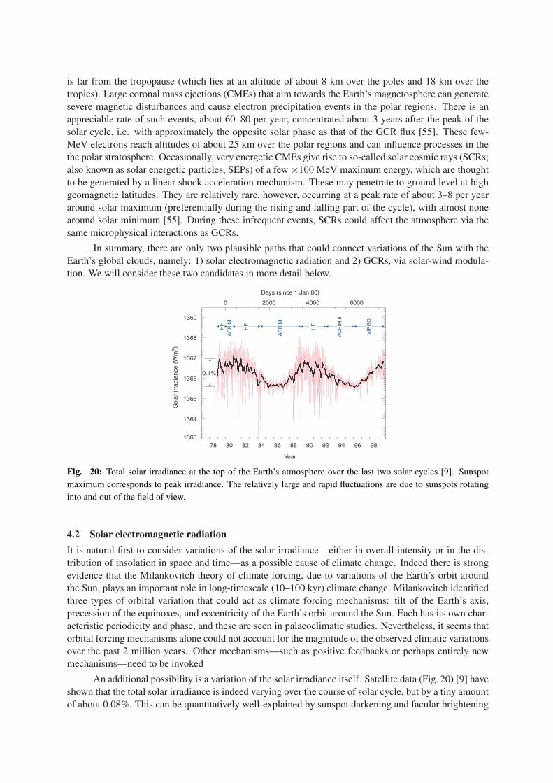
is far from the tropopause (which lies at an altitude of about 8 km over the poles and 18 km over thetropics). Large coronal mass ejections (CMEs) that aim towards the Earth’s magnetosphere can generatesevere magnetic disturbances and cause electron precipitation events in the polar regions. There is anappreciable rate of such events, about 60–80 per year, concentrated about 3 years after the peak of thesolar cycle, i.e. with approximately the opposite solar phase as that of the GCR flux [55]. These few-MeV electrons reach altitudes of about 25 km over the polar regions and can influence processes in thethe polar stratosphere. Occasionally, very energetic CMEs give rise to so-called solar cosmic rays (SCRs;also known as solar energetic particles, SEPs) of a few ×100 MeV maximum energy, which are thoughtto be generated by a linear shock acceleration mechanism. These may penetrate to ground level at highgeomagnetic latitudes. They are relatively rare, however, occurring at a peak rate of about 3–8 per yeararound solar maximum (preferentially during the rising and falling part of the cycle), with almost nonearound solar minimum [55]. During these infrequent events, SCRs could affect the atmosphere via thesame microphysical interactions as GCRs.

In summary, there are only two plausible paths that could connect variations of the Sun with theEarth’s global clouds, namely: 1) solar electromagnetic radiation and 2) GCRs, via solar-wind modula-tion. We will consider these two candidates in more detail below.

1363

1364

1365

1366

1367

1368

1369

Sol

ar ir

radi

ance

(W

m2 )

Year

0 2000 4000 6000

Days (since 1 Jan 80)

HF

AC

RIM

I

HF

AC

RIM

I

HF

AC

RIM

II

VIR

GO

78 80 82 84 86 88 90 92 94 96 98

0.1%

Fig. 20: Total solar irradiance at the top of the Earth’s atmosphere over the last two solar cycles [9]. Sunspotmaximum corresponds to peak irradiance. The relatively large and rapid fluctuations are due to sunspots rotatinginto and out of the field of view.

4.2 Solar electromagnetic radiation

It is natural first to consider variations of the solar irradiance—either in overall intensity or in the dis-tribution of insolation in space and time—as a possible cause of climate change. Indeed there is strongevidence that the Milankovitch theory of climate forcing, due to variations of the Earth’s orbit aroundthe Sun, plays an important role in long-timescale (10–100 kyr) climate change. Milankovitch identifiedthree types of orbital variation that could act as climate forcing mechanisms: tilt of the Earth’s axis,precession of the equinoxes, and eccentricity of the Earth’s orbit around the Sun. Each has its own char-acteristic periodicity and phase, and these are seen in palaeoclimatic studies. Nevertheless, it seems thatorbital forcing mechanisms alone could not account for the magnitude of the observed climatic variationsover the past 2 million years. Other mechanisms—such as positive feedbacks or perhaps entirely newmechanisms—need to be invoked

An additional possibility is a variation of the solar irradiance itself. Satellite data (Fig. 20) [9] haveshown that the total solar irradiance is indeed varying over the course of solar cycle, but by a tiny amountof about 0.08%. This can be quantitatively well-explained by sunspot darkening and facular brightening

0.1%

Wavelength (nm)102

104

102

100

10-2

1.0

0.1

0.01

0.001

10-4

103 104 105

Sol

ar ir

radi

ance

(m

W m

-2 n

m-1

) ~30km altitude cutoff

Sol

ar c

ycle

var

iatio

n(m

ax-m

in)/

max

spectral irradiance(top of atmosphere)

spectralvariability

0 km

O2 O3 H2O & CO2

UV VIS IR

Fig. 21: Wavelength dependence of the solar irradiance at the top of the atmosphere, and its variation from sunspotminimum to maximum. Also shown is the solar spectrum at the Earth’s surface after absorption by the atmosphere.

[56]. Together with measurements of cycling stars similar to our Sun, this had led to estimates of longer-term changes of solar irradiance that appear to be too small to account for the observed climate changes(§1). Attention has therefore focussed on changes of the ultra violet (UV) component of the solar spec-trum [57] which, although it carries only a small fraction of the total energy (about 0.1%), shows a muchlarger variation of several per cent over the solar cycle (Fig. 21).

The UV wavelengths are absorbed at altitudes above 30 km by oxygen (<240 nm wavelength) andozone (200–300 nm), and cause measurable heating of the thin atmosphere in the upper stratosphere. Apositive feedback mechanism exists since the increased UV creates more ozone, although the fractionalchange is small (about 1–2% from solar minimum to maximum). Modelling reproduces these changes,and studies (e.g. ref. [58]) suggest that circulation changes initially introduced in the stratosphere by thisheating can affect circulation at lower altitudes in the troposphere, and therefore can in principle influencecloudiness. It is clearly important to investigate this mechanism further with more experimental andmodelling studies.

4.3 Cosmic rays, via solar wind modulation

The other candidate link between solar variability and the Earth’s climate is via GCRs, which are mod-ulated by the solar wind. In contrast with solar UV radiation, GCRs directly penetrate the lower tropo-sphere where the cloud variation is observed, and they have an appreciable intensity variation over thesolar cycle.

4.3.1 Solar wind characteristics:

The solar wind is a continuous outward flow of plasma (mainly protons and electrons, with about 5%heavier ions) from the Sun’s corona. As a consequence of its high electrical conductivity, a weakmagnetic field is ‘frozen’ into the plasma. The solar wind follows the Parker spiral trajectories outover the huge volume of the heliosphere to distances of 50–100 AU, well beyond the orbit of Nep-tune. At the Earth’s orbit it has a velocity of 350–800 km s−1 (β = 0.001–0.003), an intensity of(0.5–5)·108 particles cm−2 s−1, and a magnetic field of about 5 · 10−5 Gauss. The main sources of thesolar wind on the Sun’s surface include large regions of open magnetic flux known as coronal holes; re-gions on the photosphere at the boundaries of the supergranulation cells, where magnetic reconnectionsoccur; and coronal mass ejections.

The sunspots themselves are but a visible indication of a high state of magnetic activity of theSun, when the solar wind is strong. Sunspots are areas of the Sun’s photosphere where strong local

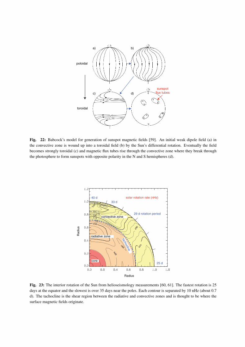
poloidal

toroidal

sunspotflux tubes

a) b)

c) d)

Fig. 22: Babcock’s model for generation of sunspot magnetic fields [59]. An initial weak dipole field (a) inthe convective zone is wound up into a toroidal field (b) by the Sun’s differential rotation. Eventually the fieldbecomes strongly toroidal (c) and magnetic flux tubes rise through the convective zone where they break throughthe photosphere to form sunspots with opposite polarity in the N and S hemispheres (d).

solar rotation rate (nHz)

Radius

Rad

ius

25 d

40 d

29 d rotation period

33 d

core

convective zone

radiative zone tachocline

Fig. 23: The interior rotation of the Sun from helioseismology measurements [60, 61]. The fastest rotation is 25days at the equator and the slowest is over 35 days near the poles. Each contour is separated by 10 nHz (about 0.7d). The tachocline is the shear region between the radiative and convective zones and is thought to be where thesurface magnetic fields originate.

magnetic fields emerge vertically. The fields are typically about 2500 Gauss, to be compared with amean quiescent photospheric field of below a few Gauss. They appear dark because their temperatureis about half of the surrounding photosphere (3,000 K compared with 5,800 K). They are generated(Fig. 22) by the differential rotation of the Sun with respect to latitude and depth: at the surface, onerevolution takes 25 days at the equator and over 35 days near the poles (Fig. 23). This transforms thequiescent dipole field into a toroidal field and eventually creates ‘knots’ of strong localised fields. Theseknots may penetrate the photosphere to form sunspots, which appear cooler due to modification of thenormal convective motions of the plasma by the strong magnetic fields. The sunspots first appear athigh latitudes and then gradually migrate towards the equator. They eventually disappear by magneticrecombination, leaving a quiescent dipole field once more (but of opposite polarity). The half-cycle fromdipole to toroidal and back to (reversed) dipole field is termed the solar, or sunspot, cycle and takes about11 years on average.

The key to solar variability is a fundamental understanding of the complex solar magnetic fields.How are they generated by the dynamo and what causes their quasi-periodic behaviour? Dynamo actioninvolves the conversion of kinetic energy into magnetic energy by the inductive effects of fluid motionin an electrically conducting fluid—the solar plasma. Babcock’s qualitative picture of the solar dynamo(outlined in Fig. 22) has been known for over 40 years. But it has only been recently with the exquisitehelioseismology measurements of GONG and other experiments, and with data from the high-precisionspectrometers and detectors on board SOHO, Ulysses, Yohkoh, TRACE and other satellites, that greatadvances are being made. For example, it appears that the tachocline (Fig. 23) plays an essential role inthe solar dynamo, and is the primary region for generation of the magnetic flux before it rises throughthe convective zone. Also, from high-resolution movies taken of the photosphere and corona, it appearsthat the dynamics of magnetic flux bundles, and their reconnections, are key to understanding the energysource that heats the solar corona and accelerates the solar wind.

4.3.2 Modulation of galactic cosmic rays by the solar wind:

Cosmic rays are generated by supernovae and other energetic sources in our galaxy and beyond. Onentering the heliosphere, charged cosmic rays are deflected by the magnetic fields of the solar wind.The transport problem of the GCRs through the heliosphere was first solved by Parker [62] and involvesseveral processes of which the dominant is scattering off the magnetic irregularities, which producesa random walk or diffusion effect. It has been shown theoretically [63] that the effect on the energyof a charged cosmic ray particle in passing through the heliosphere is equivalent to that produced bya heliocentric retarding electric potential with a magnitude at the Earth’s orbit equal to the energy lostby the cosmic rays in interacting with the solar wind. This retarding potential varies between about1000 MV during periods of very high solar activity and zero during grand minima such as the MaunderMinimum. The solar wind therefore partly shields the Earth from the lower energy GCRs and affects theflux at energies below about 10 GeV. The effective retarding potential over the present eleven-year solarcycle averages about 550 MV, ranging from about 450 MV at the minimum to 850 MV at maximum.This leads to a distinct solar modulation of the GCR intensity (Fig. 24).

The geomagnetic field also partially shields the Earth from GCRs. The dipole field imposes aminimum vertical momentum of about 13 GeV/c at the equator, 3 GeV/c at mid latitudes, and fallingessentially to zero at the geomagnetic poles. In consequence, the GCR intensity is about a factor 3.6higher at the poles than at the equator, and there is a more marked solar cycle variation at higher latitudes.Over the solar cycle, the variation of GCR intensity at the top of the atmosphere is about 15%, globallyaveraged, and ranges from ∼5% near the geomagnetic equator to ∼50% at the poles.

At lower altitudes both the GCR intensity and its fractional solar modulation decrease. These areconsequences of the absorption of low energy GCRs and their secondary particles by the atmosphericmaterial, which totals about 11 nuclear interaction lengths. Balloon measurements (Fig. 25) show solarcycle variations of about 10% at low altitudes around 3 km (for a 2.4 GeV/c rigidity cutoff).

solarmaxima:

2120cycle 19

22

Fig. 24: Balloon measurements of the cosmic ray intensity at shower maximum (15–20 km altitude) for the period1957–1998, measured by the Lebedev Physical Institute. The curves correspond to four different locations for theballoon flights: Mirny-Antarctica (0.03 GeV/c rigidity cutoff), Murmansk (0.6 GeV/c), Moscow (2.4 GeV/c) andAlma-Ata (6.7 GeV/c). Due to atmospheric absorption, the data of Murmansk and Mirny practically coincide witheach other. The approximate times of the sunspot maxima for the last 4 solar cycles are indicated.

8 kmaltititude

22

10%(3km)

Year

1960 1970 1980 1990 2000

solar maxima:cycle 19 20 21

3 kmaltititude

0.070

0.075

0.080

0.085

0.090

GC

R in

tens

ity a

t 3km

, I (

cm-2

s-1

)

0.095

0.45

0.50

0.55

0.60

0.65

0.70G

CR

inte

nsity

at 8

km

, I (

cm-2

s-1

)

Moscow(2.4 GeV/c rigidity cutoff)

Fig. 25: Balloon measurements of the GCR intensity at 3 km and 8 km altitudes from 1957 to 2000 (2.4 GeV/crigidity cutoff), measured by the Lebedev Physical Institute. The approximate dates of the sunspot maxima for thelast 4 solar cycles are indicated.

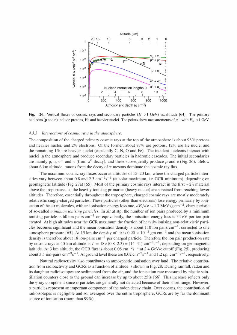
Atmospheric depth (g cm-2)

Nuclear interaction lengths, λ

0 200 400 600 800 1000

Ver

tical

flux

(cm

-2 s

-1 s

r-1 )

10-6

10-5

10-4

10-3

10-2

10-1

1

Altitude (km)

20 15 10 5 3 2 1 0

νµ + νµµ+ + µ−

π+ + π−

p + n

e+ + e−

2 4 6 8 10

Fig. 26: Vertical fluxes of cosmic rays and secondary particles (E >1 GeV) vs. altitude [64]. The primarynucleons (p and n) include protons, He and heavier nuclei. The points show measurements of µ− with Eµ >1 GeV.

4.3.3 Interactions of cosmic rays in the atmosphere:

The composition of the charged primary cosmic rays at the top of the atmosphere is about 98% protonsand heavier nuclei, and 2% electrons. Of the former, about 87% are protons, 12% are He nuclei andthe remaining 1% are heavier nuclei (especially C, N, O and Fe). The incident nucleons interact withnuclei in the atmosphere and produce secondary particles in hadronic cascades. The initial secondariesare mainly p, n, π± and γ (from π0 decay), and these subsequently produce µ and e (Fig. 26). Belowabout 6 km altitude, muons from the decay of π mesons dominate the cosmic ray flux.

The maximum cosmic ray fluxes occur at altitudes of 15–20 km, where the charged particle inten-sities vary between about 0.8 and 2.3 cm−2s−1 (at solar maximum, i.e. GCR minimum), depending ongeomagnetic latitude (Fig. 27a) [65]. Most of the primary cosmic rays interact in the first ∼2λ materialabove the tropopause, so the heavily ionising primaries (heavy nuclei) are screened from reaching loweraltitudes. Therefore, essentially throughout the troposphere, charged cosmic rays are mostly moderatelyrelativistic singly-charged particles. These particles (other than electrons) lose energy primarily by ioni-sation of the air molecules, with an ionisation energy loss rate, dE/dx∼ 1.7 MeV /g cm−2, characteristicof so-called minimum ionising particles. In air at stp, the number of ion pairs produced by a minimumionising particle is 60 ion-pairs cm−1 or, equivalently, the ionisation energy loss is 34 eV per ion paircreated. At high altitudes near the GCR maximum the fraction of heavily-ionising non-relativistic parti-cles becomes significant and the mean ionisation density is about 110 ion pairs cm−1, corrected to oneatmosphere pressure [65]. At 15 km the density of air is 0.20 × 10−3 gm cm−3 and the mean ionisationdensity is therefore about 18 ion-pairs cm−1 per charged particle. Therefore the ion pair production rateby cosmic rays at 15 km altitude is I = 18×(0.8–2.3) = (14–41) cm−3s−1, depending on geomagneticlatitude. At 3 km altitude, the GCR flux is about 0.08 cm−2s−1 at 2.4 GeV/c cutoff (Fig. 25), producingabout 3.5 ion-pairs cm−3s−1. At ground level these are 0.02 cm−2s−1 and 1.2 i.p. cm−3s−1, respectively.

Natural radioactivity also contributes to atmospheric ionisation over land. The relative contribu-tion from radioactivity and GCRs as a function of altitude is shown in Fig. 28. During rainfall, radon andits daughter radioisotopes are sedimented from the air, and the ionisation rate measured by plastic scin-tillation counters close to the ground can increase by up to about 25% [66]. This increase reflects onlythe γ ray component since α particles are generally not detected because of their short range. However,α particles represent an important component of the radon decay chain. Over oceans, the contribution ofradioisotopes is negligible and so, averaged over the entire troposphere, GCRs are by far the dominantsource of ionisation (more than 99%).

a)

b)

Charged particle intensity (cm-2s-1)

Negative small ion concentration (x1000 cm-3)

Alti

tude

(km

)A

ltitu

de (

km)

0 0.5 1.0 1.5 2.0 2.5

0 1 2 3 40

5

10

15

20

25

30

35

0

5

10

15

20

25

30

350.03 GeV/c3.3 GeV/c5.2 GeV/c17.3 GeV/c

0.03 GeV/c3.3 GeV/c5.3 GeV/c17.3 GeV/c

Fig. 27: a) The charged particle intensity and b) the negative small ion concentration vs. altitude, measured atseveral latitudes with cutoff rigidities, Rc, as indicated. The data were recorded by Lebedev Physical Institute [65]in or near 1990, corresponding to a sunspot maximum (but without solar proton events), i.e. during a cosmic rayminimum. The horizontal bars show the typical experimental statistical errors.

0

10

20

30

40

0 1 2 3

Altitude (km)

Rel

ativ

e fr

actio

n (%

)

radioactivity/GCRrelative ionisation

(over land)

Fig. 28: Relative fraction of atmospheric ionisation from radioactivity and from GCRs as a function of altitude,over land.

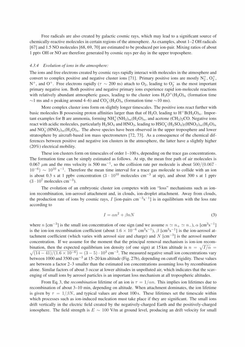
Free radicals are also created by galactic cosmic rays, which may lead to a significant source ofchemically-reactive molecules in certain regions of the atmosphere. As examples, about 1–2 OH radicals[67] and 1.5 NO molecules [68, 69, 70] are estimated to be produced per ion-pair. Mixing ratios of about1 pptv OH or NO are therefore generated by cosmic rays per day in the upper troposphere.

4.3.4 Evolution of ions in the atmosphere:

The ions and free electrons created by cosmic rays rapidly interact with molecules in the atmosphere andconvert to complex positive and negative cluster ions [71]. Primary positive ions are mostly N+

2 , O+2 ,

N+, and O+. Free electrons rapidly (τ ∼ 200 ns) attach to O2, leading to O−2 as the most important

primary negative ion. Both positive and negative primary ions experience rapid ion-molecule reactionswith relatively abundant atmospheric gases, leading to the cluster ions H3O+(H2O)n (formation time∼1 ms and n peaking around 4–6) and CO−

3 (H2O)n (formation time ∼10 ms).

More complex cluster ions form on slightly longer timescales. The positive ions react further withbasic molecules B possessing proton affinities larger than that of H2O, leading to H+B(H2O)n. Impor-tant examples for B are ammonia, forming NH+

4 (NH3)m(H2O)n, and acetone (CH3)2CO. Negative ionsreact with acidic molecules, particularly H2SO4 and HNO3, leading to HSO−

4 (H2SO4)l(HNO3)m(H2O)nand NO−

3 (HNO3)m(H2O)n. The above species have been observed in the upper troposphere and lowerstratosphere by aircraft-based ion mass spectrometers [72, 73]. As a consequence of the chemical dif-ferences between positive and negative ion clusters in the atmosphere, the latter have a slightly higher(20%) electrical mobility.

These ion clusters form on timescales of order 1–100 s, depending on the trace gas concentrations.The formation time can be simply estimated as follows. At stp, the mean free path of air molecules is0.067 µm and the rms velocity is 500 ms−1, so the collision rate per molecule is about 500/(0.067 ·10−6) ∼ 1010 s−1. Therefore the mean time interval for a trace gas molecule to collide with an ionis about 0.3 s at 1 ppbv concentration (3 · 1010 molecules cm−3 at stp), and about 300 s at 1 pptv(3 · 107 molecules cm−3).

The evolution of an embryonic cluster ion competes with ion “loss” mechanisms such as ion-ion recombination, ion-aerosol attachment and, in clouds, ion-droplet attachment. Away from clouds,the production rate of ions by cosmic rays, I [ion-pairs cm−3s−1] is in equilibrium with the loss rateaccording to

I = αn2 + βnN (3)

where n [cm−3] is the small ion concentration of one sign (and we assume n n+ n−), α [cm3s−1]is the ion-ion recombination coefficient (about 1.6 × 10−6 cm3s−1), β [cm3s−1] is the ion-aerosol at-tachment coefficient (which varies with aerosol size and charge) and N [cm−3] is the aerosol numberconcentration. If we assume for the moment that the principal removal mechanism is ion-ion recom-bination, then the expected equilibrium ion density (of one sign) at 15 km altitude is n =

√I/α =√

(14 − 41)/(1.6 × 10−6) = (3 − 5) · 103 cm−3. The measured negative small ion concentrations varybetween 1000 and 3500 cm−3 at 15–20 km altitude (Fig. 27b), depending on cutoff rigidity. These valuesare between a factor 2–3 smaller than the estimated ion concentrations assuming loss by recombinationalone. Similar factors of about 3 occur at lower altitudes in unpolluted air, which indicates that the scav-enging of small ions by aerosol particles is an important loss mechanism at all tropospheric altitudes.

From Eq. 3, the recombination lifetime of an ion is τ = 1/αn. This implies ion lifetimes due torecombination of about 3–10 min, depending on altitude. When attachment dominates, the ion lifetimeis given by τ = 1/βN , and typical values are about 100 s. These lifetimes set the timescale withinwhich processes such as ion-induced nucleation must take place if they are significant. The small ionsdrift vertically in the electric field created by the negatively-charged Earth and the positively-chargedionosphere. The field strength is E ∼ 100 V/m at ground level, producing an drift velocity for small

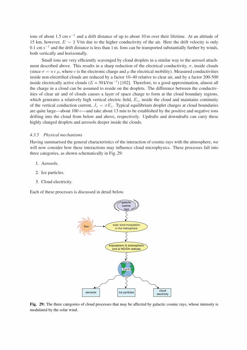
ions of about 1.5 cm s−1 and a drift distance of up to about 10 m over their lifetime. At an altitude of15 km, however, E ∼ 2 V/m due to the higher conductivity of the air. Here the drift velocity is only0.1 cm s−1 and the drift distance is less than 1 m. Ions can be transported substantially further by winds,both vertically and horizontally.

Small ions are very efficiently scavenged by cloud droplets in a similar way to the aerosol attach-ment described above. This results in a sharp reduction of the electrical conductivity, σ, inside clouds(since σ = n e µ, where e is the electronic charge and µ the electrical mobility). Measured conductivitiesinside non-electrified clouds are reduced by a factor 10–40 relative to clear air, and by a factor 200-500inside electrically active clouds (E = 30 kVm−1) [102]. Therefore, to a good approximation, almost allthe charge in a cloud can be assumed to reside on the droplets. The difference between the conductiv-ities of clear air and of clouds causes a layer of space charge to form at the cloud boundary regions,which generates a relatively high vertical electric field, Ez , inside the cloud and maintains continuityof the vertical conduction current, Jz = σEz . Typical equilibrium droplet charges at cloud boundariesare quite large—about 100 e—and take about 13 min to be established by the positive and negative ionsdrifting into the cloud from below and above, respectively. Updrafts and downdrafts can carry thesehighly charged droplets and aerosols deeper inside the clouds.

4.3.5 Physical mechanisms

Having summarised the general characteristics of the interaction of cosmic rays with the atmosphere, wewill now consider how these interactions may influence cloud microphysics. These processes fall intothree categories, as shown schematically in Fig. 29:

1. Aerosols.

2. Ice particles.

3. Cloud electricity.

Each of these processes is discussed in detail below.

galacticcosmic

rays

solar wind modulationin the heliosphere

tropospheric & stratosphericions & NO/OH radicals

aerosolscloud

electricityice particles

Sun

Earth

Fig. 29: The three categories of cloud processes that may be affected by galactic cosmic rays, whose intensity ismodulated by the solar wind.

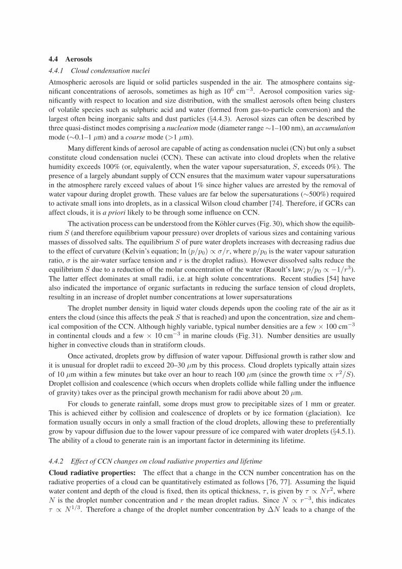
4.4 Aerosols

4.4.1 Cloud condensation nuclei

Atmospheric aerosols are liquid or solid particles suspended in the air. The atmosphere contains sig-nificant concentrations of aerosols, sometimes as high as 106 cm−3. Aerosol composition varies sig-nificantly with respect to location and size distribution, with the smallest aerosols often being clustersof volatile species such as sulphuric acid and water (formed from gas-to-particle conversion) and thelargest often being inorganic salts and dust particles (§4.4.3). Aerosol sizes can often be described bythree quasi-distinct modes comprising a nucleation mode (diameter range ∼1–100 nm), an accumulationmode (∼0.1–1 µm) and a coarse mode (>1 µm).

Many different kinds of aerosol are capable of acting as condensation nuclei (CN) but only a subsetconstitute cloud condensation nuclei (CCN). These can activate into cloud droplets when the relativehumidity exceeds 100% (or, equivalently, when the water vapour supersaturation, S, exceeds 0%). Thepresence of a largely abundant supply of CCN ensures that the maximum water vapour supersaturationsin the atmosphere rarely exceed values of about 1% since higher values are arrested by the removal ofwater vapour during droplet growth. These values are far below the supersaturations (∼500%) requiredto activate small ions into droplets, as in a classical Wilson cloud chamber [74]. Therefore, if GCRs canaffect clouds, it is a priori likely to be through some influence on CCN.

The activation process can be understood from the Kohler curves (Fig. 30), which show the equilib-rium S (and therefore equilibrium vapour pressure) over droplets of various sizes and containing variousmasses of dissolved salts. The equilibrium S of pure water droplets increases with decreasing radius dueto the effect of curvature (Kelvin’s equation; ln (p/p0) ∝ σ/r, where p/p0 is the water vapour saturationratio, σ is the air-water surface tension and r is the droplet radius). However dissolved salts reduce theequilibrium S due to a reduction of the molar concentration of the water (Raoult’s law; p/p0 ∝ −1/r3).The latter effect dominates at small radii, i.e. at high solute concentrations. Recent studies [54] havealso indicated the importance of organic surfactants in reducing the surface tension of cloud droplets,resulting in an increase of droplet number concentrations at lower supersaturations

The droplet number density in liquid water clouds depends upon the cooling rate of the air as itenters the cloud (since this affects the peak S that is reached) and upon the concentration, size and chem-ical composition of the CCN. Although highly variable, typical number densities are a few × 100 cm−3

in continental clouds and a few × 10 cm−3 in marine clouds (Fig. 31). Number densities are usuallyhigher in convective clouds than in stratiform clouds.

Once activated, droplets grow by diffusion of water vapour. Diffusional growth is rather slow andit is unusual for droplet radii to exceed 20–30 µm by this process. Cloud droplets typically attain sizesof 10 µm within a few minutes but take over an hour to reach 100 µm (since the growth time ∝ r2/S).Droplet collision and coalescence (which occurs when droplets collide while falling under the influenceof gravity) takes over as the principal growth mechanism for radii above about 20 µm.

For clouds to generate rainfall, some drops must grow to precipitable sizes of 1 mm or greater.This is achieved either by collision and coalescence of droplets or by ice formation (glaciation). Iceformation usually occurs in only a small fraction of the cloud droplets, allowing these to preferentiallygrow by vapour diffusion due to the lower vapour pressure of ice compared with water droplets (§4.5.1).The ability of a cloud to generate rain is an important factor in determining its lifetime.

4.4.2 Effect of CCN changes on cloud radiative properties and lifetime

Cloud radiative properties: The effect that a change in the CCN number concentration has on theradiative properties of a cloud can be quantitatively estimated as follows [76, 77]. Assuming the liquidwater content and depth of the cloud is fixed, then its optical thickness, τ , is given by τ ∝ Nr2, whereN is the droplet number concentration and r the mean droplet radius. Since N ∝ r−3, this indicatesτ ∝ N1/3. Therefore a change of the droplet number concentration by ∆N leads to a change of the

critical supersaturation for 0.1 µm (NH4)2SO4

293 K

0.5 µm: dry diameter(NH4)2SO4

0.1 µm0.05 µm

Droplet diameter (µm)0.1 1 10 100

Wat

er v

apou

r su

pers

atur

atio

n (%

)

0.0

-0.1

-0.2

-0.3

0.1

0.2

0.3

0.4

0.5

0.6

0.7

0.8

pure water(Kelvin's eq.)

solute effect (Raoult's law)

Fig. 30: Kohler curves showing the equilibrium water vapour supersaturation at 293 K for droplets of pure water(dotted curve) and for droplets containing various masses of dissolved (NH4)2SO4 (solid curves) vs. diameter of thedroplet [75]. The water vapour supersaturation, S (%) = (p/p0−1)·100, where p is the partial pressure of the watervapour and p0 is the saturated vapour pressure over a plane surface of water at this temperature. In the indicatedexample, an ambient water vapour S of 0.15% (dashed line) exceeds the critical value for all ammonium sulphateaerosols with dry diameter ≥ 0.1 µm. These aerosols will therefore activate and grow into cloud droplets, whereassmaller aerosols remain as unactivated haze particles. Droplets below their corresponding equilibrium curve willshrink by evaporation whereas those above will grow by condensation (the indicated droplets correspond, forexample, to a dry diameter of 0.05 µm).

10

100

1,000

10,000

0 0.2 0.4 0.6 0.8 1 1.2

Water vapour supersaturation (%)

CC

N c

once

ntra

tion

(cm

-3)

Marine (Australia)

Continental (typical)

Continental (Australia)Continental (Buffalo, NY)

Atlantic

Hawaii

Fig. 31: Measurements of CCN concentrations at several sites: marine (solid curves) and continental (dashedcurves) as a function of the water vapour supersaturation [75]. The CCN concentrations are equal to the clouddroplet concentrations at a given supersaturation.

optical thickness by ∆τ given by

∆τ

τ=

13· ∆N

N(4)

The albedo (reflectivity), A, of a cloud is the fraction of incident radiation that is reflected into thebackward hemisphere. For the scattering of solar radiation by clouds [76, 77],

A ≈ τ

τ + 6.7(5)

Differentiating Eq. 5 and combining with Eq. 4 gives,

∆A

A= (1 − A) · ∆N

N(6)

The rather thin stratiform clouds that cover an appreciable fraction of the Earth’s surface, and especiallymarine regions, have an albedo of about 0.5 and a droplet number concentration of about 100 cm−3

or less (Fig. 31). Equation 6 shows that these clouds are very sensitive to changes in the CCN numberconcentration; their reflectance changes by 0.5% or more per single additional cloud droplet per cubiccentimetre of air! This in turn indicates that GCR-induced changes in the CCN number concentrationof only a few per cent could produce significant effects on the radiative properties of such clouds. Asa numerical example, Figure 32 shows the variation of cloud reflectivity with cloud depth and clouddroplet number density for a fixed liquid water content of 0.3 g m−3 (most data confirm that there is littleor no dependence of liquid water content on cloud droplet number density).

0

0.2

0.4

0.6

0.8

1.0

Ref

lect

ivity

10 100 1000

Cloud droplet number concentration (cm )-3

cloud thickness (m)

50

100

500

1500

Fig. 32: The variation of cloud albedo with cloud thickness and droplet number concentration for a fixed liquidwater content of 0.3 g m−3 [78].

Cloud lifetime: The second effect of an increase in CCN concentration is to suppress rainfall andthereby to increase cloud lifetime. This has been observed over oceans in ship tracks [79] and, recently,also over land [80]. The latter study used NOAA satellite data to investigate clouds that formed down-wind of industrial sites located in pristine areas. The otherwise uniform cloud data from these regionswas streaked with bright (highly reflective) cloud plumes from the industrial sites. The droplets in theseplumes were found to be more numerous than the nearby regions and of a smaller diameter—typicallyless than 10 µm and therefore below the threshold size for them to coalesce efficiently and precipitate.In contrast the droplets outside the plumes measured more than 25 µm in diameter. The high reflectivityof the plumes resulted from the high droplet number density at fixed liquid water content (Fig. 32). Inde-pendent analysis of data from the Tropical Rainfall Measuring Mission confirmed that these plumes didindeed produce less rain and therefore had a longer lifetime than clouds in the nearby regions.

aerosolparticles

primary gaseousorganic emissions

gas-phasephotochemistry

gas-phasephotochemistry

gas-phasephotochemistry

condensableorganic vapours

primary particulateorganic emissions

SO2/DMS emissions

H2SO4

primary H2SO4 emissions

H2O vapour

NH3 emissions

NOx emissions

HNO3

primary particulateinorganic emissions(dust, carbon, etc.)

sea salt

gas-to-particlenucleationGCR

GCR GCR

secondary aerosol sources

primary aerosol sources

Fig. 33: The main sources of atmospheric aerosols. These are classified as primary if they are injected directlyinto the air or secondary if they result from gas-to-particle conversion in the atmosphere. The processes that maybe affected by galactic cosmic rays (GCRs) are indicated by wavy arrows.

4.4.3 Production and loss of atmospheric aerosols

The main sources of atmospheric aerosols are summarised in Fig. 33. Aerosols are classified as eitherprimary or secondary, and they may be of either natural or anthropogenic origin. Primary aerosols arethose injected directly into the air (e.g. by wind erosion, sea spray, pollen, etc.). Secondary aerosols arethose created by gas-to-particle nucleation of vapour molecules. Inorganic aerosols are usually weaklyacidic, with the most common aqueous cationic components being H+, ammonium and sodium, andwith common anionic components being sulphate, chloride and nitrate. Such aerosols are hygroscopic.Aerosols can also be partly or wholly composed of organic compounds derived from plant waxes andcombustion sources. These aerosols may be either hygrophobic or hygroscopic. Secondary aerosolsmay originate from emissions of non-condensable vapours followed by gas-phase chemical conversioninto condensable (i.e. low vapour pressure) aerosol precursors, e.g. SO2 oxidation to H2SO4. Cloudsare an important source as well as sink of aerosols since they provide efficient sites for the scavengingand chemical processing of aerosols and aerosol precursors. These pathways for aerosol production areshown in Fig. 34.

Once formed, aerosols have both a direct and an indirect effect of the climate by their influenceon radiative forcing. The direct effect is due to scattering and absorption of the incoming shortwaveradiation. Absorptive aerosols such as black carbon have a net positive forcing (warming) and reflectiveones such as hygroscopic aerosols have a net negative forcing. The indirect effect is due to a change

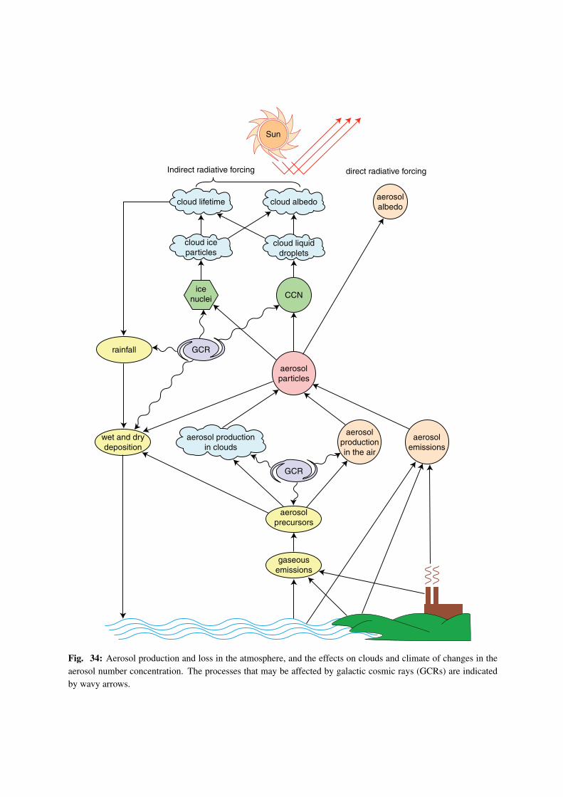
GCR

GCR

gaseousemissions

aerosolprecursors

wet and drydeposition

rainfall

CCN

cloud liquiddroplets

cloud albedocloud lifetime

Indirect radiative forcing direct radiative forcing

icenuclei

cloud iceparticles

aerosolproductionin the air

aerosolemissions

aerosol productionin clouds

aerosolparticles

aerosolalbedo

Sun

Fig. 34: Aerosol production and loss in the atmosphere, and the effects on clouds and climate of changes in theaerosol number concentration. The processes that may be affected by galactic cosmic rays (GCRs) are indicatedby wavy arrows.

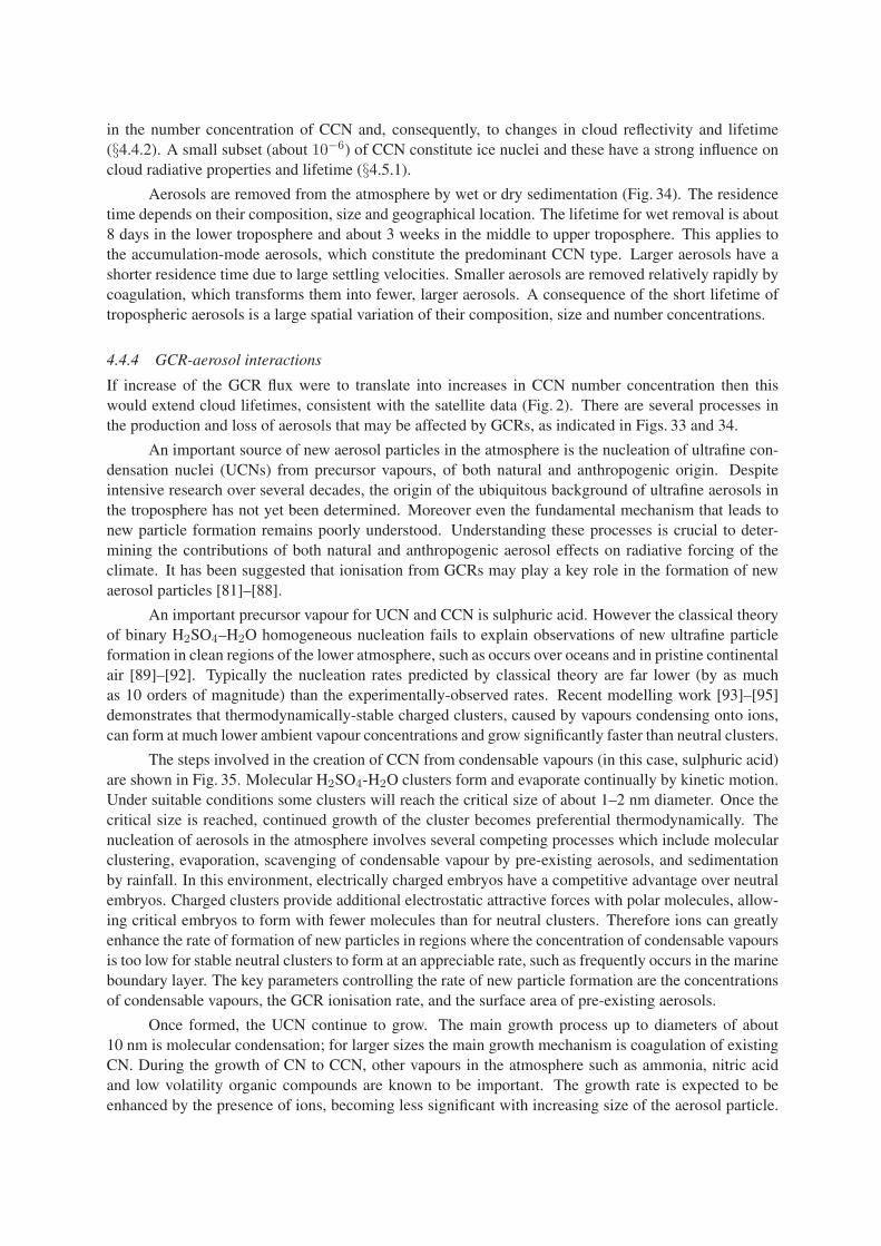
in the number concentration of CCN and, consequently, to changes in cloud reflectivity and lifetime(§4.4.2). A small subset (about 10−6) of CCN constitute ice nuclei and these have a strong influence oncloud radiative properties and lifetime (§4.5.1).

Aerosols are removed from the atmosphere by wet or dry sedimentation (Fig. 34). The residencetime depends on their composition, size and geographical location. The lifetime for wet removal is about8 days in the lower troposphere and about 3 weeks in the middle to upper troposphere. This applies tothe accumulation-mode aerosols, which constitute the predominant CCN type. Larger aerosols have ashorter residence time due to large settling velocities. Smaller aerosols are removed relatively rapidly bycoagulation, which transforms them into fewer, larger aerosols. A consequence of the short lifetime oftropospheric aerosols is a large spatial variation of their composition, size and number concentrations.

4.4.4 GCR-aerosol interactions

If increase of the GCR flux were to translate into increases in CCN number concentration then thiswould extend cloud lifetimes, consistent with the satellite data (Fig. 2). There are several processes inthe production and loss of aerosols that may be affected by GCRs, as indicated in Figs. 33 and 34.

An important source of new aerosol particles in the atmosphere is the nucleation of ultrafine con-densation nuclei (UCNs) from precursor vapours, of both natural and anthropogenic origin. Despiteintensive research over several decades, the origin of the ubiquitous background of ultrafine aerosols inthe troposphere has not yet been determined. Moreover even the fundamental mechanism that leads tonew particle formation remains poorly understood. Understanding these processes is crucial to deter-mining the contributions of both natural and anthropogenic aerosol effects on radiative forcing of theclimate. It has been suggested that ionisation from GCRs may play a key role in the formation of newaerosol particles [81]–[88].

An important precursor vapour for UCN and CCN is sulphuric acid. However the classical theoryof binary H2SO4–H2O homogeneous nucleation fails to explain observations of new ultrafine particleformation in clean regions of the lower atmosphere, such as occurs over oceans and in pristine continentalair [89]–[92]. Typically the nucleation rates predicted by classical theory are far lower (by as muchas 10 orders of magnitude) than the experimentally-observed rates. Recent modelling work [93]–[95]demonstrates that thermodynamically-stable charged clusters, caused by vapours condensing onto ions,can form at much lower ambient vapour concentrations and grow significantly faster than neutral clusters.

The steps involved in the creation of CCN from condensable vapours (in this case, sulphuric acid)are shown in Fig. 35. Molecular H2SO4-H2O clusters form and evaporate continually by kinetic motion.Under suitable conditions some clusters will reach the critical size of about 1–2 nm diameter. Once thecritical size is reached, continued growth of the cluster becomes preferential thermodynamically. Thenucleation of aerosols in the atmosphere involves several competing processes which include molecularclustering, evaporation, scavenging of condensable vapour by pre-existing aerosols, and sedimentationby rainfall. In this environment, electrically charged embryos have a competitive advantage over neutralembryos. Charged clusters provide additional electrostatic attractive forces with polar molecules, allow-ing critical embryos to form with fewer molecules than for neutral clusters. Therefore ions can greatlyenhance the rate of formation of new particles in regions where the concentration of condensable vapoursis too low for stable neutral clusters to form at an appreciable rate, such as frequently occurs in the marineboundary layer. The key parameters controlling the rate of new particle formation are the concentrationsof condensable vapours, the GCR ionisation rate, and the surface area of pre-existing aerosols.

Once formed, the UCN continue to grow. The main growth process up to diameters of about10 nm is molecular condensation; for larger sizes the main growth mechanism is coagulation of existingCN. During the growth of CN to CCN, other vapours in the atmosphere such as ammonia, nitric acidand low volatility organic compounds are known to be important. The growth rate is expected to beenhanced by the presence of ions, becoming less significant with increasing size of the aerosol particle.

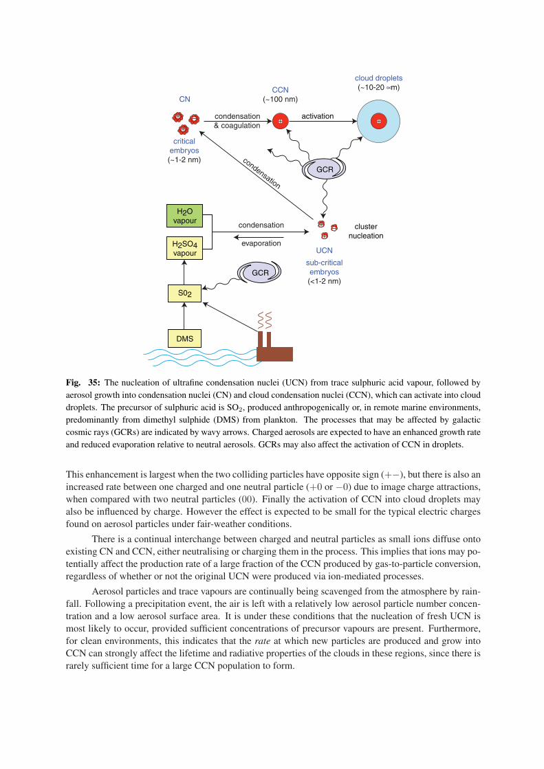
S02

DMS

activation

+

+–

criticalembryos(~1-2 nm)

sub-criticalembryos(<1-2 nm)

condensation

evaporation

condensation

CCN(~100 nm)

cloud droplets(~10-20 µm)

clusternucleation

H2SO4vapour

H2Ovapour

condensation& coagulation

++ +

+–

CN

UCN

GCR

GCR

Fig. 35: The nucleation of ultrafine condensation nuclei (UCN) from trace sulphuric acid vapour, followed byaerosol growth into condensation nuclei (CN) and cloud condensation nuclei (CCN), which can activate into clouddroplets. The precursor of sulphuric acid is SO2, produced anthropogenically or, in remote marine environments,predominantly from dimethyl sulphide (DMS) from plankton. The processes that may be affected by galacticcosmic rays (GCRs) are indicated by wavy arrows. Charged aerosols are expected to have an enhanced growth rateand reduced evaporation relative to neutral aerosols. GCRs may also affect the activation of CCN in droplets.

This enhancement is largest when the two colliding particles have opposite sign (+−), but there is also anincreased rate between one charged and one neutral particle (+0 or −0) due to image charge attractions,when compared with two neutral particles (00). Finally the activation of CCN into cloud droplets mayalso be influenced by charge. However the effect is expected to be small for the typical electric chargesfound on aerosol particles under fair-weather conditions.

There is a continual interchange between charged and neutral particles as small ions diffuse ontoexisting CN and CCN, either neutralising or charging them in the process. This implies that ions may po-tentially affect the production rate of a large fraction of the CCN produced by gas-to-particle conversion,regardless of whether or not the original UCN were produced via ion-mediated processes.

Aerosol particles and trace vapours are continually being scavenged from the atmosphere by rain-fall. Following a precipitation event, the air is left with a relatively low aerosol particle number concen-tration and a low aerosol surface area. It is under these conditions that the nucleation of fresh UCN ismost likely to occur, provided sufficient concentrations of precursor vapours are present. Furthermore,for clean environments, this indicates that the rate at which new particles are produced and grow intoCCN can strongly affect the lifetime and radiative properties of the clouds in these regions, since there israrely sufficient time for a large CCN population to form.

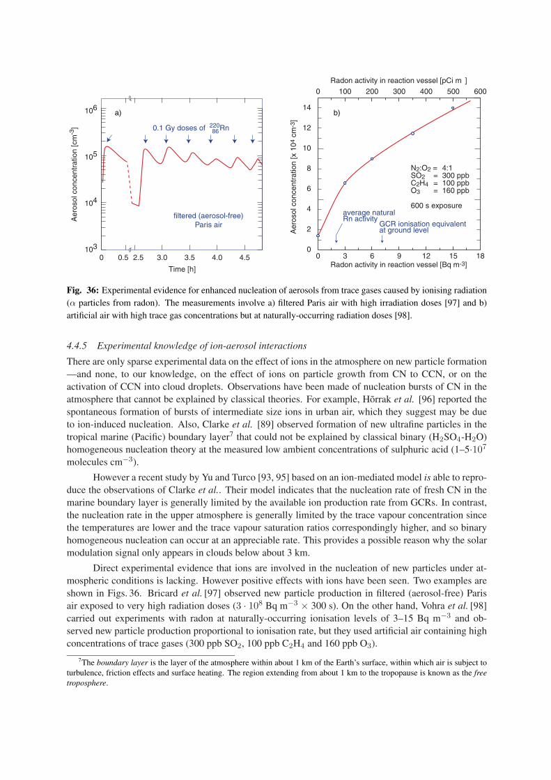
filtered (aerosol-free)Paris air

a) b)

103

104

105

106

Aer

osol

con

cent

ratio

n [c

m-3

]

Time [h]

0 0.5 2.5 3.0 3.5 4.0 4.5

0.1 Gy doses of 220Rn86

0

0 100 200 300 400 500 600

0 3 6 9 12 15 18

2

4

6

8

10

12

14

Radon activity in reaction vessel [Bq m-3]

Radon activity in reaction vessel [pCi m ]

Aer

osol

con

cent

ratio

n [x

104

cm

-3]

average naturalRn activity

GCR ionisation equivalentat ground level

N2:O2 = 4:1SO2 = 300 ppbC2H4 = 100 ppbO3 = 160 ppb

600 s exposure

Fig. 36: Experimental evidence for enhanced nucleation of aerosols from trace gases caused by ionising radiation(α particles from radon). The measurements involve a) filtered Paris air with high irradiation doses [97] and b)artificial air with high trace gas concentrations but at naturally-occurring radiation doses [98].

4.4.5 Experimental knowledge of ion-aerosol interactions

There are only sparse experimental data on the effect of ions in the atmosphere on new particle formation—and none, to our knowledge, on the effect of ions on particle growth from CN to CCN, or on theactivation of CCN into cloud droplets. Observations have been made of nucleation bursts of CN in theatmosphere that cannot be explained by classical theories. For example, Horrak et al. [96] reported thespontaneous formation of bursts of intermediate size ions in urban air, which they suggest may be dueto ion-induced nucleation. Also, Clarke et al. [89] observed formation of new ultrafine particles in thetropical marine (Pacific) boundary layer7 that could not be explained by classical binary (H2SO4-H2O)homogeneous nucleation theory at the measured low ambient concentrations of sulphuric acid (1–5·107

molecules cm−3).

However a recent study by Yu and Turco [93, 95] based on an ion-mediated model is able to repro-duce the observations of Clarke et al.. Their model indicates that the nucleation rate of fresh CN in themarine boundary layer is generally limited by the available ion production rate from GCRs. In contrast,the nucleation rate in the upper atmosphere is generally limited by the trace vapour concentration sincethe temperatures are lower and the trace vapour saturation ratios correspondingly higher, and so binaryhomogeneous nucleation can occur at an appreciable rate. This provides a possible reason why the solarmodulation signal only appears in clouds below about 3 km.

Direct experimental evidence that ions are involved in the nucleation of new particles under at-mospheric conditions is lacking. However positive effects with ions have been seen. Two examples areshown in Figs. 36. Bricard et al. [97] observed new particle production in filtered (aerosol-free) Parisair exposed to very high radiation doses (3 · 108 Bq m−3 × 300 s). On the other hand, Vohra et al. [98]carried out experiments with radon at naturally-occurring ionisation levels of 3–15 Bq m−3 and ob-served new particle production proportional to ionisation rate, but they used artificial air containing highconcentrations of trace gases (300 ppb SO2, 100 ppb C2H4 and 160 ppb O3).

7The boundary layer is the layer of the atmosphere within about 1 km of the Earth’s surface, within which air is subject toturbulence, friction effects and surface heating. The region extending from about 1 km to the tropopause is known as the freetroposphere.

4.5 Ice particles

4.5.1 Overview

The second class of processes by which GCRs may affect clouds concerns ice particles. The formationof ice in clouds is important for several reasons:

1. In mixed-phase clouds, ice particles grow rapidly at the expense of liquid water droplets. Whenthe water vapour supersaturation relative to liquid water is 0%, the supersaturation relative to ice ismuch higher, as large as 50% (Fig. 37). Since supersaturation is the ‘driving force’ that determinesgrowth rate, the ice particles grow rapidly, reducing the ambient supersaturation and causing theliquid water droplets to evaporate. The ice particles rapidly grow to a size where they sedimentand ‘rain-out’ the clouds below.8

2. The freezing of supercooled water releases latent heat, which affects cloud dynamics.

3. Ice particles modify the radiative properties of clouds, both by increasing sedimentation and bychanging the reflectivity (particles that are larger and crystalline). As an indication of the impor-tance of ice particles, the IPCC finds that uncertainties in the fraction of frozen water in cloudsresults in differences of up to 17 Wm−2 in their estimates of globally-averaged cloud forcing [49].

0 -10 -20 -30 -40

Temperature (oC)

0

10

20

30

40

50

Sup

ersa

tura

tion

rela

tive

to ic

e (%

)

0% SS relative to liquid water

Fig. 37: The supersaturation relative to ice for water vapour that is in equilibrium with liquid water at thetemperature indicated on the x axis. In the temperature range from 0C to -40C liquid water can exist in asupercooled state in the absence of an ice nucleus. Below -40C, water freezes homogeneously, i.e. without needof a distinct ice nucleus.

Once a cloud extends to altitudes where the temperature is below 0C, ice crystals may form.Two phase transitions can lead to ice formation (Fig. 38): (a) the direct deposition (sublimation) of watervapour to ice and (b and c) the freezing of a supercooled liquid droplet. The latter may occur either bythe transformation of a supercooled liquid droplet into an ice particle (freezing nucleation) or collisionof a supercooled liquid droplet with an ice nuclei (contact nucleation). The relative importance of thesethree freezing modes has not yet been established. The freezing may proceed either on a suitable ice nu-cleus (IN) (heterogeneous nucleation), as shown in Fig. 38, or else occur with pure water (homogeneousnucleation). For homogeneous nucleation to take place, a statistical fluctuation of the water moleculesmust occur to produce a stable, ice-like structure that can serve as an ice nucleus. For typical clouddroplet dimensions (∼10 µm), homogeneous nucleation occurs at about -40C. Therefore, for clouds inthe temperature range between 0C and -40C, ice particle nucleation is heterogeneous and requires asuitable IN.

Field measurements show that clouds contains a great deal of supercooled liquid water in thistemperature range, since ice nuclei are very rare in the atmosphere. The IN number concentration is

8This is the principle behind cloud-seeding, in which a suitable ice nucleus material, e.g. AgI, induces the freezing ofsupercooled cloud droplets.

supercooledliquid droplet

supercooledliquid droplet

ice particle

ice nucleus

GCR

c) contact nucleation

a) deposition nucleation

b) freezing nucleation

Fig. 38: Processes for ice particle formation in clouds, involving a) deposition nucleation: the direct sublimationof water vapour to the solid phase on an ice nucleus, b) freezing nucleation: condensation of a supercooled liquiddroplet on a suitable ice nucleus, followed by freezing as the temperature falls, and c) contact nucleation: thefreezing of a supercooled liquid droplet (already formed on a CCN) by external contact with an ice nucleus. GCRsmay affect the efficiency of CCNs to act as ice nuclei and may directly affect freezing nucleation.

typically ∼1 /litre at about -20C, increasing by a factor 10 for each 4C of additional cooling. Thismay be compared with a CCN number concentration of ∼ 106 /litre or, said another way, only one ina million CCN constitutes a suitable IN at -20C. Identifying such particles is a difficult task, and INremain poorly understood. However efficient IN are generally insoluble in water and have a chemicalbonding and crystallographic structure similar to ice. Examples include various insoluble salts (such asAgI), certain clay particles, various organic materials and even bacteria (which is surprising since neitherof the last two have a crystalline structure). Although some IN have been identified, the number of iceparticles found in clouds often exceeds the measured IN concentration by several orders of magnitude.

Part of this discrepancy can be attributed to ice multiplication in secondary processes. When adroplet freezes at temperature between about -5C and -10C, mechanical stresses lead to the ejection ofsmall ice fragments, which in turn act as efficient ice nuclei. Collisions between dense graupel particlesand fragile dendritic crystals also generate ice splinters. However the understanding of these processes isalso poor. Recent measurements [99] suggest that freezing-thawing cycles may be an important factor inIN production. These authors found that the thermal history of droplets affects the temperatures at whichthey eventually freeze. In summary many observations of ice particle in clouds cannot be explainedquantitatively and, in particular, there appears to be a great lack of IN to account for the observed numbersof ice particles in clouds.

4.5.2 GCR-ice particle interactions

Enhanced heterogeneous ice nucleation by electrification has been proposed by several workers. Forexample, Tinsley [100, 101] has proposed that cosmic rays have an important influence on cloud micro-physics and climate through the following sequence of events. Cosmic rays generate ionisation in theatmosphere and determine the magnitude of the vertical conduction current, Jz (§4.6.2). This currentgenerates highly charged droplets (>∼100 e) at the upper and lower boundaries of clouds due to the ac-cumulation of space charge (§4.3.4). When these droplets evaporate they leave behind highly chargedaerosols which are coated with extra sulphates and insoluble organic compounds scavenged while thedroplet existed. (It has been shown that neither electric charge nor aerosol material is not lost when adroplet evaporates.) These highly charged and coated “evaporation nuclei” constitute efficient ice nuclei,either by deposition nucleation or by contact nucleation. The presence of charge enhances collisions ofthe evaporation nuclei with other liquid droplets by “electroscavenging” (§4.6.2), thereby generating iceparticles in clouds.

If this sequence of events is correct, it would imply that increased GCR intensity leads to in-

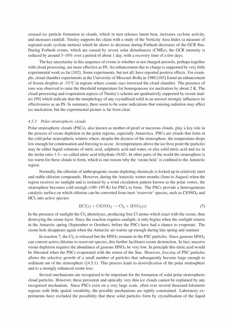
creased ice particle formation in clouds, which in turn releases latent heat, increases cyclone activity,and increases rainfall. Tinsley supports his claim with a study of the Vorticity Area Index (a measure ofregional-scale cyclone motion) which he shows to decrease during Forbush decreases of the GCR flux.During Forbush events, which are caused by severe solar disturbances (CMEs), the GCR intensity isreduced by around 3–10% over a period of about 1 day, with a recovery time of a few days.

The key uncertainty in this sequence of events is whether or not charged aerosols, perhaps togetherwith cloud processing, are more effective as IN. An enhancement due to charge is supported by very littleexperimental work so far [102]. Some experiments, but not all, have reported positive effects. For exam-ple, cloud chamber experiments at the University of Missouri-Rolla in 1980 [103] found an enhancementof frozen droplets at -33C in regions where cosmic rays traversed the cloud chamber. The presence ofions was observed to raise the threshold temperature for homogeneous ice nucleation by about 2 K. Thecloud-processing and evaporation aspects of Tinsley’s scheme are qualitatively supported by recent stud-ies [99] which indicate that the morphology of any crystallised solid in an aerosol strongly influences itseffectiveness as an IN. In summary, there seem to be some indications that ionising radiation may affectice nucleation, but the experimental picture is far from clear.

4.5.3 Polar stratospheric clouds

Polar stratospheric clouds (PSCs), also known as mother-of-pearl or nacreous clouds, play a key role inthe process of ozone depletion in the polar regions, especially Antarctica. PSCs are clouds that form inthe cold polar stratospheric winters where, despite the dryness of the stratosphere, the temperature dropslow enough for condensation and freezing to occur. At temperatures above the ice frost point the particlesmay be either liquid solutions of nitric acid, sulphuric acid and water, or else solid nitric acid and ice inthe molar ratio 1:3—so called nitric acid trihydrate (NAT). In other parts of the world the stratosphere istoo warm for these clouds to form, which is one reason why the ‘ozone hole’ is confined to the Antarcticregion.

Normally, the chlorine of anthropogenic ozone-depleting chemicals is locked up in relatively inertand stable chlorine compounds. However, during the Antarctic winter months (June to August) when theregion receives no sunlight and is isolated by a wind circulation pattern known as the polar vortex, thestratosphere becomes cold enough (190–195 K) for PSCs to form. The PSCs provide a heterogeneouscatalytic surface on which chlorine can be converted from inert ‘reservoir’ species, such as ClONO2 andHCl, into active species:

HCl(s) + ClONO2 → Cl2 + HNO3(s) (7)

In the presence of sunlight the Cl2 photolyses, producing free Cl atoms which react with the ozone, thusdestroying the ozone layer. Since the reaction requires sunlight, it only begins when the sunlight returnsin the Antarctic spring (September to October), before the PSCs have had a chance to evaporate. Theozone hole disappears again when the Antarctic air warms up enough during late spring and summer

In reaction 7, the Cl2 is released but the HNO3 remains in the PSC particles. Since gaseous HNO3

can convert active chlorine to reservoir species, this further facilitates ozone destruction. In fact, massiveozone depletion requires the abundance of gaseous HNO3 be very low. In principle this nitric acid wouldbe liberated when the PSCs evaporated with the return of the Sun. However, freezing of PSC particlesallows the selective growth of a small number of particles that subsequently become large enough tosediment out of the stratosphere (§4.5.1). This process leads to denitrification of the polar stratosphereand to a strongly enhanced ozone loss.

Several mechanisms are recognised to be important for the formation of solid polar stratosphericcloud particles. However, these persistent and optically very thin ice clouds cannot be explained by anyrecognised mechanism. Since PSCs exist on a very large scale, often over several thousand kilometreregions with little spatial variability, the possible mechanisms are tightly constrained. Laboratory ex-periments have excluded the possibility that these solid particles form by crystallisation of the liquid

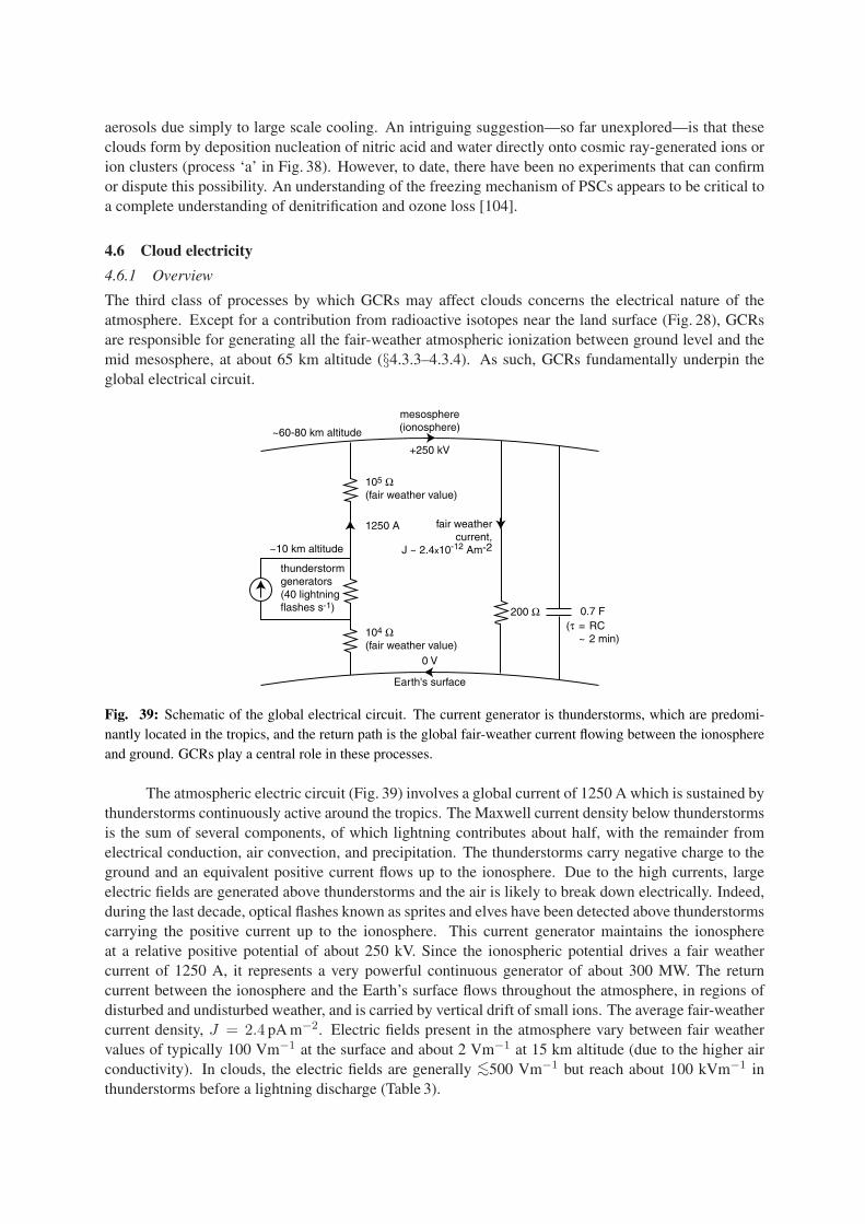
aerosols due simply to large scale cooling. An intriguing suggestion—so far unexplored—is that theseclouds form by deposition nucleation of nitric acid and water directly onto cosmic ray-generated ions orion clusters (process ‘a’ in Fig. 38). However, to date, there have been no experiments that can confirmor dispute this possibility. An understanding of the freezing mechanism of PSCs appears to be critical toa complete understanding of denitrification and ozone loss [104].

4.6 Cloud electricity

4.6.1 Overview

The third class of processes by which GCRs may affect clouds concerns the electrical nature of theatmosphere. Except for a contribution from radioactive isotopes near the land surface (Fig. 28), GCRsare responsible for generating all the fair-weather atmospheric ionization between ground level and themid mesosphere, at about 65 km altitude (§4.3.3–4.3.4). As such, GCRs fundamentally underpin theglobal electrical circuit.

0.7 F

Earth's surface

mesosphere(ionosphere)

fair weathercurrent,

J ~ 2.4x10-12 Am-2

1250 A

+250 kV

0 V

~10 km altitude

~60-80 km altitude

(τ = RC ~ 2 min)

105 Ω(fair weather value)

104 Ω(fair weather value)

200 Ω

thunderstormgenerators(40 lightningflashes s-1)

Fig. 39: Schematic of the global electrical circuit. The current generator is thunderstorms, which are predomi-nantly located in the tropics, and the return path is the global fair-weather current flowing between the ionosphereand ground. GCRs play a central role in these processes.

The atmospheric electric circuit (Fig. 39) involves a global current of 1250 A which is sustained bythunderstorms continuously active around the tropics. The Maxwell current density below thunderstormsis the sum of several components, of which lightning contributes about half, with the remainder fromelectrical conduction, air convection, and precipitation. The thunderstorms carry negative charge to theground and an equivalent positive current flows up to the ionosphere. Due to the high currents, largeelectric fields are generated above thunderstorms and the air is likely to break down electrically. Indeed,during the last decade, optical flashes known as sprites and elves have been detected above thunderstormscarrying the positive current up to the ionosphere. This current generator maintains the ionosphereat a relative positive potential of about 250 kV. Since the ionospheric potential drives a fair weathercurrent of 1250 A, it represents a very powerful continuous generator of about 300 MW. The returncurrent between the ionosphere and the Earth’s surface flows throughout the atmosphere, in regions ofdisturbed and undisturbed weather, and is carried by vertical drift of small ions. The average fair-weathercurrent density, J = 2.4 pA m−2. Electric fields present in the atmosphere vary between fair weathervalues of typically 100 Vm−1 at the surface and about 2 Vm−1 at 15 km altitude (due to the higher airconductivity). In clouds, the electric fields are generally <∼500 Vm−1 but reach about 100 kVm−1 inthunderstorms before a lightning discharge (Table 3).

Table 3: Typical maximum electric fields measured inside clouds [105]. Electric fields in all types of non-thunderstorm clouds are generally <∼0.5 kVm−1. For comparison, the clear-air electric field is about 0.1 kVm−1

at ground level. The dielectric field strength of dry air at stp is 30 MVm−1, which represents the breakdown fieldstrength across plane parallel electrodes. The threshold electric fields for wet air breakdown are about 1–2 MVm−1.

Cloud type Maximum electric field

(kVm−1)

stratus 1

stratocumulus 1.5

cirrostratus 1.5

altostratus 5

nimbostratus 15

thunderstorm 100

atmosphericcurrent

lightning

0.8

1.2

1.6

2.0

1965 1970 1975 1980 1985Year

0.54

0.58

0.62

0.66

10

15

20

25

30

1988 1992 1996 2000

Year

8

9

10

11

12

GC

R in

tens

ity (

cm-2

s-1

)(8

km

alti

tude

)

GC

R io

n pa

ir ra

te (

cm-2

s-1

)(in

2-1

0 km

col

umn)

Atm

osph

eric

cur

rent

den

sity

, J(x

10-

12 A

m-2

)

b) USA

GCR

GCR

Ligh

tnin

g fr

eque

ncy

(x10

6 /y

ear)a) Polar region

Fig. 40: a) Solar-cycle variation of the atmospheric current density, J , and the GCR intensity, both in the polarregion, [107] and b) frequency of lightning recorded in the United Sates and change of GCR intensity for 1988–1999 [108].

4.6.2 GCR - cloud-electricity interactions

Global electrical circuit: By their effect on the ion pair concentration and, perhaps, on lightning fre-quency, GCRs can in principle affect the atmospheric conductivity, σ, the ionospheric potential, theatmospheric current density, J , and the atmospheric electric field, Ez . A study of the variation of atmo-spheric current density in the polar region over the period 1965–1985 (Fig. 40a) [107] shows evidencefor a solar modulation. The increase of J around the minimum of the solar cycle is consistent with theincreased conductivity of the air due to the higher GCR intensity. However, there is a second inferenceto be made: there must be a simultaneous increase of the current source, i.e. of lightning frequency, inorder to sustain the higher net flow of fair-weather charge between the ionosphere and the ground. Somedirect evidence that supports this is seen in Fig. 40b) [108]. This suggests that the efficiency of chargeseparation in thunder clouds may be influenced by the ionisation concentration from GCRs (a mechanismthat is consistent with this picture is discussed below). However other studies of a possible relationshipbetween solar activity and the frequency of thunderstorms or lightning have been made, and the resultsare not conclusive with some reporting a positive correlation, some a negative correlation and some noneof any significance (see, for example ref. [106] and references therein). Therefore more experimentaldata are required to clarify the situation.

Since lightning is the dominant source of NOx in the marine troposphere, if GCRs do indeedaffect lightning frequency, it would imply they also modulate the production of this important reactivetrace radical in the troposphere [109]. Note that this production mechanism for NOx (and OH radicals)occurs both below thunderclouds (due to lightning) and above them (due to sprites and elves; § 4.6.1).

Rainfall: Stozhkov et al. have studied the influence of Forbush decreases of GCR intensity on precip-itation in Brazil and in the former Soviet Union [55, 110]. The combined experimental data for around70 Forbush events (Fig. 41a) indicate a decrease of rainfall of (17 ± 3)% on the day of the Forbush de-crease. These authors have also studied ground-level solar proton events (solar cosmic rays), where thecosmic ray intensity increases for a period of about a day due to high energy solar events (Fig. 41b). Heretoo they find some evidence for an effect, (13 ± 5)% (53 combined events), and with a consistent sign,namely an increase of rainfall. In a separate study of Forbush events, Pudovkin and Veretenenko havereported [111] a correlated short-term decrease of cloudiness using data obtained visually in a narrowrange of latitudes (60N–64N), which is consistent with the global satellite observations (§2).

-20

-10

0

10

Change in rainfall (%)

-15

-10

-5

0

5

10

15

-30 -20 -10 10 20 30Day

-35 -25 -15 -5 5 15 25 35Day

Day 0 = Forbush onset

Day 0 = SCR event

Change in rainfall (%)

a)

b)

Fig. 41: Variation of rainfall recorded in the former Soviet Union and Brazil during short-term changes the cosmicray intensity [55]. The relative change in rainfall in the days spanning a) decreases of the cosmic ray intensity dueto Forbush events (70 combined events) and b) increases of the cosmic ray intensity due to ground-level solarcosmic ray events (53 combined events).

These data suggest that GCR ionisation may affect the precipitation efficiency of clouds. Onecandidate physical mechanism is an enhanced formation of ice particles (§4.5). Another is the increasedefficiency of droplet growth by collision and coalescence, which is the dominant process by which clouddroplets grow in size from cloud droplets (about 20 µm diameter) into raindrops (about 1 mm). Clouddroplets become charged by the diffusion of small ions. Measurements indicate that the mean electroniccharge on a non-thunderstorm cloud droplet is approximately represented by q(e) = 4.1 r2(µm2), wherer is the droplet radius [102]. In thunderstorm conditions, the charge is about an order of magnitude larger,q ∼ 40 r2. The presence of charge is expected to produce large increases of coalescence efficiency dueto image charge forces, which are always attractive at sufficiently close distances (see, for example,Fig. 42). This process has been termed “electroscavenging” [100, 101].

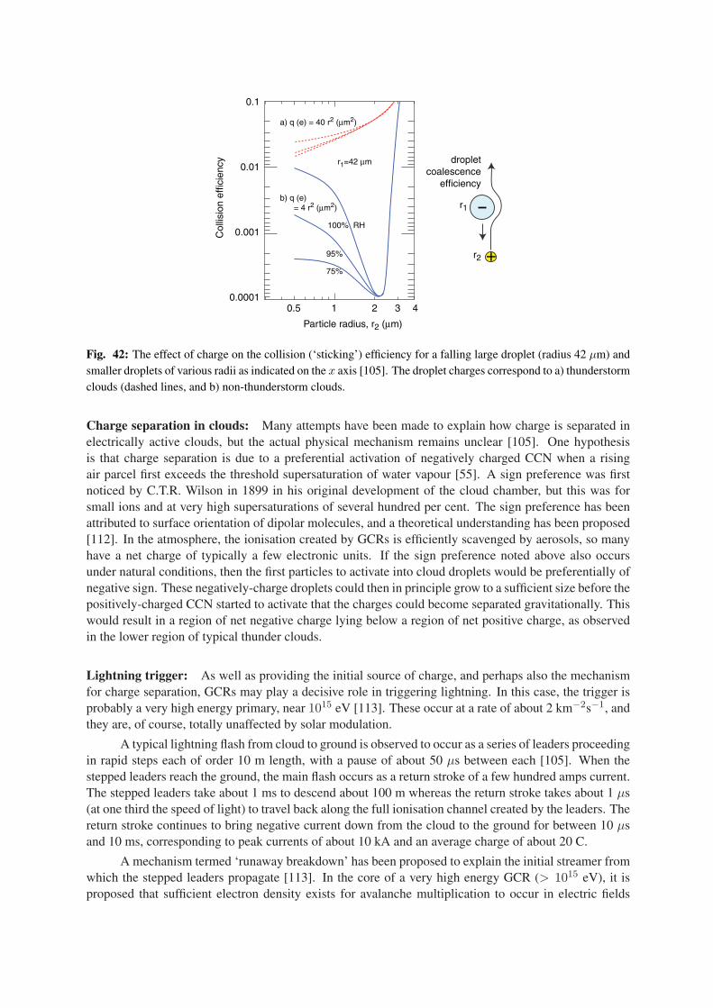
100% RH

95%

75%

0.1

0.01

0.001

0.0001

Col

lisio

n ef

ficie

ncy

Particle radius, r2 (µm)

0.5 1 2 3 4

r1=42 µm

r1

r2

a) q (e) = 40 r2 (µm2)

b) q (e) = 4 r2 (µm2)

+

dropletcoalescence

efficiency

Fig. 42: The effect of charge on the collision (‘sticking’) efficiency for a falling large droplet (radius 42 µm) andsmaller droplets of various radii as indicated on the x axis [105]. The droplet charges correspond to a) thunderstormclouds (dashed lines, and b) non-thunderstorm clouds.

Charge separation in clouds: Many attempts have been made to explain how charge is separated inelectrically active clouds, but the actual physical mechanism remains unclear [105]. One hypothesisis that charge separation is due to a preferential activation of negatively charged CCN when a risingair parcel first exceeds the threshold supersaturation of water vapour [55]. A sign preference was firstnoticed by C.T.R. Wilson in 1899 in his original development of the cloud chamber, but this was forsmall ions and at very high supersaturations of several hundred per cent. The sign preference has beenattributed to surface orientation of dipolar molecules, and a theoretical understanding has been proposed[112]. In the atmosphere, the ionisation created by GCRs is efficiently scavenged by aerosols, so manyhave a net charge of typically a few electronic units. If the sign preference noted above also occursunder natural conditions, then the first particles to activate into cloud droplets would be preferentially ofnegative sign. These negatively-charge droplets could then in principle grow to a sufficient size before thepositively-charged CCN started to activate that the charges could become separated gravitationally. Thiswould result in a region of net negative charge lying below a region of net positive charge, as observedin the lower region of typical thunder clouds.

Lightning trigger: As well as providing the initial source of charge, and perhaps also the mechanismfor charge separation, GCRs may play a decisive role in triggering lightning. In this case, the trigger isprobably a very high energy primary, near 1015 eV [113]. These occur at a rate of about 2 km−2s−1, andthey are, of course, totally unaffected by solar modulation.

A typical lightning flash from cloud to ground is observed to occur as a series of leaders proceedingin rapid steps each of order 10 m length, with a pause of about 50 µs between each [105]. When thestepped leaders reach the ground, the main flash occurs as a return stroke of a few hundred amps current.The stepped leaders take about 1 ms to descend about 100 m whereas the return stroke takes about 1 µs(at one third the speed of light) to travel back along the full ionisation channel created by the leaders. Thereturn stroke continues to bring negative current down from the cloud to the ground for between 10 µsand 10 ms, corresponding to peak currents of about 10 kA and an average charge of about 20 C.

A mechanism termed ‘runaway breakdown’ has been proposed to explain the initial streamer fromwhich the stepped leaders propagate [113]. In the core of a very high energy GCR (> 1015 eV), it isproposed that sufficient electron density exists for avalanche multiplication to occur in electric fields

of 100–200 kVm−1, which are typical of thunderstorm clouds (Table 3) but well below the thresholdfields for conventional damp air breakdown (1–2 MVm−1). The avalanche polarizes the local plasmaand thereby increases the electric field in a positive feedback. This raises the electron density to the pointwhere a short streamer forms, which then triggers the first leader. A distinctive signature of the runawaybreakdown mechanism is the appearance of X rays of energy around 50–100 keV starting with the firststepped leader, around 1 ms before the lightning discharge, which are caused by electron bremsstrahlungin the highly conductive plasma (long mean free path). Such X rays have recently been observed inlightning storms [114, 115].

Finally we comment that the association of an ultra high energy GCR shower with a lightningdischarge may help explain the phenomena of ‘rain gushes’. The latter are the familiar dramatic increasein precipitation arriving at the ground shortly after nearby lightning [105]. It is possible that rain gushesresult from a sudden increase of droplet coalescence efficiency due to a sharp rise of ionisation, asdescribed above (Fig. 42). Various attempts have been made to explain how the ionisation generatedby a lightning flash could rapidly diffuse laterally over a sufficiently large area, but none is convincing.However, since the transverse width of an ultra high energy GCR shower is about 100 m, then thecombination of the initial ionisation, a triggered lightning flash, X ray emission and absorption, andsome mild electrical activity over the full width of the GCR shower may together generate sufficientionisation to cause the rain gush over a ∼100 m-wide region.

5 THE CLOUD FACILITY

5.1 Concept

The basic concept of the CLOUD experiment (Figs. 43 and 44) is to investigate the microphysics of GCR-cloud interactions under laboratory conditions where all the experimental parameters can be preciselycontrolled and measured. A beam from a particle accelerator provides an artificial source of ‘cosmicrays’ that is adjustable and precisely known. The beam illuminates a 0.5 m expansion cloud chamberand a 2 m reactor chamber. The chambers can be operated at any temperature and pressure in thetroposphere and stratosphere. The cloud chamber simulates the conditions inside clouds, throughout theatmosphere. The reactor chamber is important for experiments involving long beam exposures of a dayor more, and provides the reacted gas/aerosol samples for analysis by the external instrumentation—massspectrometers, particle sizers, etc. Data will be recorded under a wide variety of operating conditions,and the results compared at different beam intensities, including beam-off. In this way an unambiguousstudy of the effects of relativistic ionising particles on cloud microphysics can be carried out.

Such measurements are difficult to perform with cosmic rays in the atmosphere since the naturalintensity variations are modest and—with the exception of relatively rare Forbush decreases—they followthe slow 11-year solar cycle. Furthermore, a laboratory experiment allows full control of the gas andaerosol mixture under test and, in addition, complete physical and chemical analysis of the productsbefore, during and after beam exposure. This will greatly facilitate an understanding of the microphysicsand chemistry of any effects that are observed. The challenges of a laboratory experiment are to duplicatethe atmospheric conditions realistically and to ensure that the detector dimensions are sufficiently largethat wall effects do not influence the measurements.

Surprisingly, cloud chambers have never been operated at atmospheric conditions in a particlebeam. C.T.R. Wilson was inspired to develop the cloud chamber [74, 116] after observing meteorologicalphenomena on the mountain of Ben Nevis in 1894. He developed the cloud chamber to try to reproduceclouds in the laboratory. Although his expansion cloud chamber was crucial to the development ofnuclear and particle physics in the first half of the 20th century, and earned him the 1927 Nobel Prize inPhysics, Wilson remained fascinated by atmospheric phenomena throughout his life. Indeed he devotedthe latter part of his research life to seeking a connection between cosmic rays and clouds, and so it isperhaps a fitting tribute that a cloud chamber be proposed for the present studies.

reactor chamber

illumination/ UV lamps

liquid fluorocarbonstorage

vacuum system

piston hydraulicsystem

platform

µ beam

field cage

0 1m

cloud

cloud chamber

fan

liquid cooling pipes

vacuum layer

Fig. 43: Vertical section through the CLOUD facility showing the 0.5 m cloud chamber and 2 m reactor chamber.The beam counters are not shown.

5.2 Design considerations

5.2.1 Choice of expansion cloud chamber

There are several instruments capable of activating cloud condensation nuclei into droplets at the low wa-ter vapour supersaturations (few × 0.1%) found in clouds. Traditionally these are based on the diffusioncloud chamber or some variant thereof. All produce the necessary supersaturations over relatively smallvolumes and have inherent limitations in precision and in range of supersaturation (or, equivalently, inrange of CCN size) [117]. Expansion cloud chambers, on the other hand, can in principle produce a pre-cise and uniform supersaturation over a large volume and, moreover, maintain or dynamically adjust thesupersaturation over long periods. They are therefore uniquely suited to the CLOUD experiments, manyof which require long times for beam exposure, aerosol growth and droplet observation (§5.5.1). Expan-sion cloud chambers can also cover the full range of supersaturations between cloud conditions and thoserequired (∼500%) to activate small ions and embryonic aerosols in the nanometre size range. The phrase“in principle” is used above since the technical requirements are quite challenging (see below) and, toour knowledge, a cloud chamber with the performance proposed has not previously been built. However,the design requirements can be achieved with current technology, and extensive experience with cloudchambers has shown that they are high precision instruments. In particular, previous measurements bymembers of the CLOUD collaboration have demonstrated that the thermodynamic conditions after an

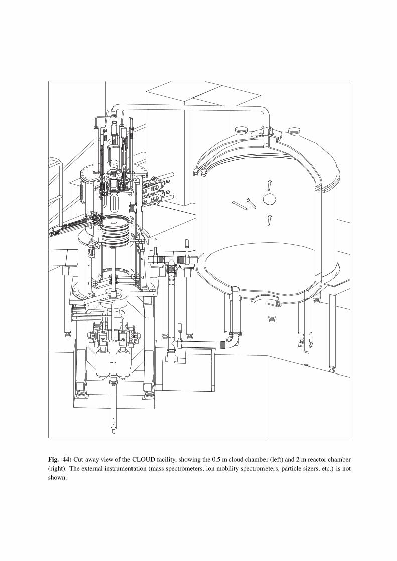
Fig. 44: Cut-away view of the CLOUD facility, showing the 0.5 m cloud chamber (left) and 2 m reactor chamber(right). The external instrumentation (mass spectrometers, ion mobility spectrometers, particle sizers, etc.) is notshown.

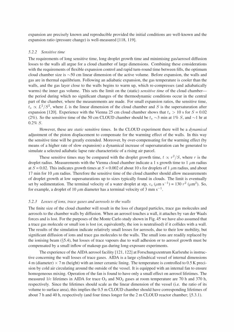
expansion are precisely known and reproducible provided the initial conditions are well-known and theexpansion ratio (pressure change) is well-measured [118, 119].

5.2.2 Sensitive time

The requirements of long sensitive time, long droplet growth time and minimising gas/aerosol diffusionlosses to the walls all argue for a cloud chamber of large dimensions. Combining these considerationswith the requirements of flexible expansion control and rapid turn-round time between fills, the optimumcloud chamber size is ∼50 cm linear dimension of the active volume. Before expansion, the walls andgas are in thermal equilibrium. Following an adiabatic expansion, the gas temperature is cooler than thewalls, and the gas layer close to the walls begins to warm up, which re-compresses (and adiabaticallywarms) the inner gas volume. This sets the limit on the (static) sensitive time of the cloud chamber—the period during which no significant changes of the thermodynamic conditions occur in the centralpart of the chamber, where the measurements are made. For small expansion ratios, the sensitive time,ts ∝ L2/S2, where L is the linear dimension of the cloud chamber and S is the supersaturation afterexpansion [120]. Experience with the Vienna 25 cm cloud chamber shows that ts > 10 s for S = 0.02(2%). So the sensitive time of the 50 cm CLOUD chamber should be ts ∼3 min at 1% S, and ∼1 hr at0.2% S.

However, these are static sensitive times. In the CLOUD experiment there will be a dynamicaladjustment of the piston displacement to compensate for the warming effect of the walls. In this waythe sensitive time will be greatly extended. Moreover, by over-compensating for the warming effect (bymeans of a higher rate of slow expansion) a dynamical increase of supersaturation can be generated tosimulate a selected adiabatic lapse rate characteristic of a rising air parcel.

These sensitive times may be compared with the droplet growth time, t ∝ r2/S, where r is thedroplet radius. Measurements with the Vienna cloud chamber indicate a 1 s growth time to 1 µm radiusat S = 0.02. This indicates growth times at S = 0.002 of about 10 s for droplets of 1 µm radius, and about17 min for 10 µm radius. Therefore the sensitive time of the cloud chamber should allow measurementsof droplet growth at low supersaturations up to sizes typically found in clouds. The limit is eventuallyset by sedimentation. The terminal velocity of a water droplet at stp, vo (µm s−1) = 130 r2 (µm2). So,for example, a droplet of 10 µm diameter has a terminal velocity of 3 mm s−1.

5.2.3 Losses of ions, trace gases and aerosols to the walls

The finite size of the cloud chamber will result in the loss of charged particles, trace gas molecules andaerosols to the chamber walls by diffusion. When an aerosol touches a wall, it attaches by van der Waalsforces and is lost. For the purposes of the Monte Carlo study shown in Fig. 45 we have also assumed thata trace gas molecule or small ion is lost (or, equivalently, the ion is neutralised) if it collides with a wall.The results of the simulation indicate relatively small losses for aerosols, due to their low mobility, butsignificant diffusion of ions and trace gas molecules to the walls. The small ions are readily replaced bythe ionising beam (§5.4), but losses of trace vapours due to wall adhesion or to aerosol growth must becompensated by a small inflow of makeup gas during long-exposure experiments.

The experience of the AIDA aerosol facility [121, 122] at Forschungszentrum Karlsruhe is instruc-tive concerning the wall losses of trace gases. AIDA is a large cylindrical vessel of internal dimensions4 m (diameter) × 7 m (height) with an inner ceramic lining. The temperature is controlled to 0.5 K preci-sion by cold air circulating around the outside of the vessel. It is equipped with an internal fan to ensurehomogeneous mixing. Operation of the fan is found to have only a small effect on aerosol lifetimes. Themeasured 1/e lifetimes in AIDA for trace O3 and NO2 gases at room temperature are 70 h and 370 h,respectively. Since the lifetimes should scale as the linear dimension of the vessel (i.e. the ratio of itsvolume to surface area), this implies the 0.5 m CLOUD chamber should have corresponding lifetimes ofabout 7 h and 40 h, respectively (and four times longer for the 2 m CLOUD reactor chamber; §5.3.1).

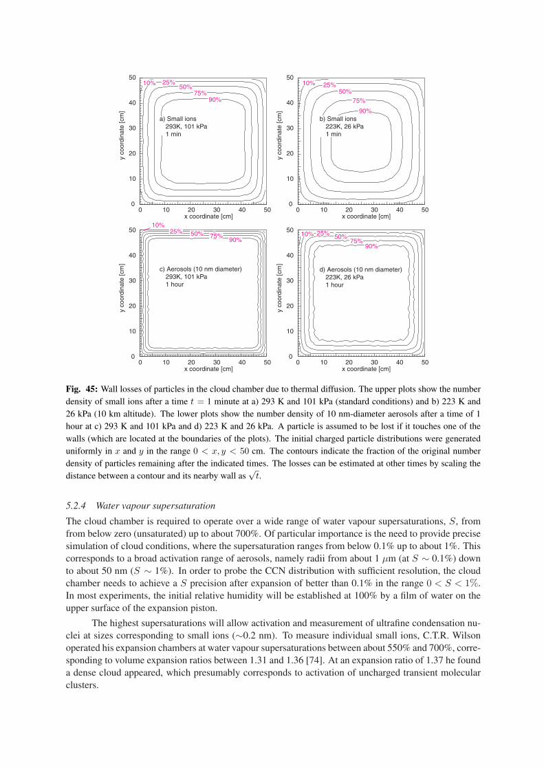
0

10

20

30

40

50

0 10 20 30 40 50

y co

ordi

nate

[cm

]

x coordinate [cm]

a) Small ions 293K, 101 kPa 1 min

b) Small ions 223K, 26 kPa 1 min

c) Aerosols (10 nm diameter) 293K, 101 kPa 1 hour

d) Aerosols (10 nm diameter) 223K, 26 kPa 1 hour

90%75%

50%25%10%

0

10

20

30

40

50

0 10 20 30 40 50

y co

ordi

nate

[cm

]

x coordinate [cm]

90%75%50%25%

10%

0

10

20

30

40

50

0 10 20 30 40 50

y co

ordi

nate

[cm

]

x coordinate [cm]

90%

75%50%

25%10%

0

10

20

30

40

50

0 10 20 30 40 50

y co

ordi

nate

[cm

]

x coordinate [cm]

90%75%

50%25%10%

Fig. 45: Wall losses of particles in the cloud chamber due to thermal diffusion. The upper plots show the numberdensity of small ions after a time t = 1 minute at a) 293 K and 101 kPa (standard conditions) and b) 223 K and26 kPa (10 km altitude). The lower plots show the number density of 10 nm-diameter aerosols after a time of 1hour at c) 293 K and 101 kPa and d) 223 K and 26 kPa. A particle is assumed to be lost if it touches one of thewalls (which are located at the boundaries of the plots). The initial charged particle distributions were generateduniformly in x and y in the range 0 < x, y < 50 cm. The contours indicate the fraction of the original numberdensity of particles remaining after the indicated times. The losses can be estimated at other times by scaling thedistance between a contour and its nearby wall as

√t.

5.2.4 Water vapour supersaturation

The cloud chamber is required to operate over a wide range of water vapour supersaturations, S, fromfrom below zero (unsaturated) up to about 700%. Of particular importance is the need to provide precisesimulation of cloud conditions, where the supersaturation ranges from below 0.1% up to about 1%. Thiscorresponds to a broad activation range of aerosols, namely radii from about 1 µm (at S ∼ 0.1%) downto about 50 nm (S ∼ 1%). In order to probe the CCN distribution with sufficient resolution, the cloudchamber needs to achieve a S precision after expansion of better than 0.1% in the range 0 < S < 1%.In most experiments, the initial relative humidity will be established at 100% by a film of water on theupper surface of the expansion piston.

The highest supersaturations will allow activation and measurement of ultrafine condensation nu-clei at sizes corresponding to small ions (∼0.2 nm). To measure individual small ions, C.T.R. Wilsonoperated his expansion chambers at water vapour supersaturations between about 550% and 700%, corre-sponding to volume expansion ratios between 1.31 and 1.36 [74]. At an expansion ratio of 1.37 he founda dense cloud appeared, which presumably corresponds to activation of uncharged transient molecularclusters.

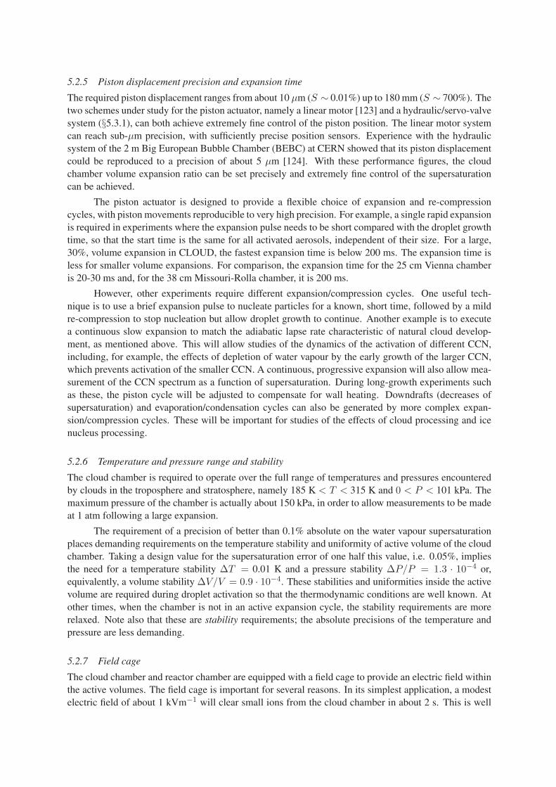
5.2.5 Piston displacement precision and expansion time

The required piston displacement ranges from about 10 µm (S ∼ 0.01%) up to 180 mm (S ∼ 700%). Thetwo schemes under study for the piston actuator, namely a linear motor [123] and a hydraulic/servo-valvesystem (§5.3.1), can both achieve extremely fine control of the piston position. The linear motor systemcan reach sub-µm precision, with sufficiently precise position sensors. Experience with the hydraulicsystem of the 2 m Big European Bubble Chamber (BEBC) at CERN showed that its piston displacementcould be reproduced to a precision of about 5 µm [124]. With these performance figures, the cloudchamber volume expansion ratio can be set precisely and extremely fine control of the supersaturationcan be achieved.

The piston actuator is designed to provide a flexible choice of expansion and re-compressioncycles, with piston movements reproducible to very high precision. For example, a single rapid expansionis required in experiments where the expansion pulse needs to be short compared with the droplet growthtime, so that the start time is the same for all activated aerosols, independent of their size. For a large,30%, volume expansion in CLOUD, the fastest expansion time is below 200 ms. The expansion time isless for smaller volume expansions. For comparison, the expansion time for the 25 cm Vienna chamberis 20-30 ms and, for the 38 cm Missouri-Rolla chamber, it is 200 ms.

However, other experiments require different expansion/compression cycles. One useful tech-nique is to use a brief expansion pulse to nucleate particles for a known, short time, followed by a mildre-compression to stop nucleation but allow droplet growth to continue. Another example is to executea continuous slow expansion to match the adiabatic lapse rate characteristic of natural cloud develop-ment, as mentioned above. This will allow studies of the dynamics of the activation of different CCN,including, for example, the effects of depletion of water vapour by the early growth of the larger CCN,which prevents activation of the smaller CCN. A continuous, progressive expansion will also allow mea-surement of the CCN spectrum as a function of supersaturation. During long-growth experiments suchas these, the piston cycle will be adjusted to compensate for wall heating. Downdrafts (decreases ofsupersaturation) and evaporation/condensation cycles can also be generated by more complex expan-sion/compression cycles. These will be important for studies of the effects of cloud processing and icenucleus processing.

5.2.6 Temperature and pressure range and stability

The cloud chamber is required to operate over the full range of temperatures and pressures encounteredby clouds in the troposphere and stratosphere, namely 185 K < T < 315 K and 0 < P < 101 kPa. Themaximum pressure of the chamber is actually about 150 kPa, in order to allow measurements to be madeat 1 atm following a large expansion.

The requirement of a precision of better than 0.1% absolute on the water vapour supersaturationplaces demanding requirements on the temperature stability and uniformity of active volume of the cloudchamber. Taking a design value for the supersaturation error of one half this value, i.e. 0.05%, impliesthe need for a temperature stability ∆T = 0.01 K and a pressure stability ∆P/P = 1.3 · 10−4 or,equivalently, a volume stability ∆V/V = 0.9 · 10−4. These stabilities and uniformities inside the activevolume are required during droplet activation so that the thermodynamic conditions are well known. Atother times, when the chamber is not in an active expansion cycle, the stability requirements are morerelaxed. Note also that these are stability requirements; the absolute precisions of the temperature andpressure are less demanding.

5.2.7 Field cage

The cloud chamber and reactor chamber are equipped with a field cage to provide an electric field withinthe active volumes. The field cage is important for several reasons. In its simplest application, a modestelectric field of about 1 kVm−1 will clear small ions from the cloud chamber in about 2 s. This is well

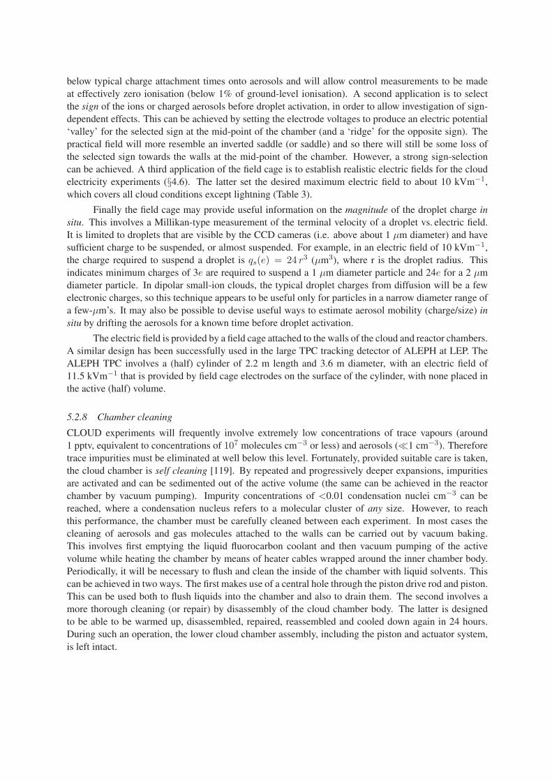
below typical charge attachment times onto aerosols and will allow control measurements to be madeat effectively zero ionisation (below 1% of ground-level ionisation). A second application is to selectthe sign of the ions or charged aerosols before droplet activation, in order to allow investigation of sign-dependent effects. This can be achieved by setting the electrode voltages to produce an electric potential‘valley’ for the selected sign at the mid-point of the chamber (and a ‘ridge’ for the opposite sign). Thepractical field will more resemble an inverted saddle (or saddle) and so there will still be some loss ofthe selected sign towards the walls at the mid-point of the chamber. However, a strong sign-selectioncan be achieved. A third application of the field cage is to establish realistic electric fields for the cloudelectricity experiments (§4.6). The latter set the desired maximum electric field to about 10 kVm−1,which covers all cloud conditions except lightning (Table 3).

Finally the field cage may provide useful information on the magnitude of the droplet charge insitu. This involves a Millikan-type measurement of the terminal velocity of a droplet vs. electric field.It is limited to droplets that are visible by the CCD cameras (i.e. above about 1 µm diameter) and havesufficient charge to be suspended, or almost suspended. For example, in an electric field of 10 kVm−1,the charge required to suspend a droplet is qs(e) = 24 r3 (µm3), where r is the droplet radius. Thisindicates minimum charges of 3e are required to suspend a 1 µm diameter particle and 24e for a 2 µmdiameter particle. In dipolar small-ion clouds, the typical droplet charges from diffusion will be a fewelectronic charges, so this technique appears to be useful only for particles in a narrow diameter range ofa few-µm’s. It may also be possible to devise useful ways to estimate aerosol mobility (charge/size) insitu by drifting the aerosols for a known time before droplet activation.

The electric field is provided by a field cage attached to the walls of the cloud and reactor chambers.A similar design has been successfully used in the large TPC tracking detector of ALEPH at LEP. TheALEPH TPC involves a (half) cylinder of 2.2 m length and 3.6 m diameter, with an electric field of11.5 kVm−1 that is provided by field cage electrodes on the surface of the cylinder, with none placed inthe active (half) volume.

5.2.8 Chamber cleaning

CLOUD experiments will frequently involve extremely low concentrations of trace vapours (around1 pptv, equivalent to concentrations of 107 molecules cm−3 or less) and aerosols (1 cm−3). Thereforetrace impurities must be eliminated at well below this level. Fortunately, provided suitable care is taken,the cloud chamber is self cleaning [119]. By repeated and progressively deeper expansions, impuritiesare activated and can be sedimented out of the active volume (the same can be achieved in the reactorchamber by vacuum pumping). Impurity concentrations of <0.01 condensation nuclei cm−3 can bereached, where a condensation nucleus refers to a molecular cluster of any size. However, to reachthis performance, the chamber must be carefully cleaned between each experiment. In most cases thecleaning of aerosols and gas molecules attached to the walls can be carried out by vacuum baking.This involves first emptying the liquid fluorocarbon coolant and then vacuum pumping of the activevolume while heating the chamber by means of heater cables wrapped around the inner chamber body.Periodically, it will be necessary to flush and clean the inside of the chamber with liquid solvents. Thiscan be achieved in two ways. The first makes use of a central hole through the piston drive rod and piston.This can be used both to flush liquids into the chamber and also to drain them. The second involves amore thorough cleaning (or repair) by disassembly of the cloud chamber body. The latter is designedto be able to be warmed up, disassembled, repaired, reassembled and cooled down again in 24 hours.During such an operation, the lower cloud chamber assembly, including the piston and actuator system,is left intact.

condensation particlecounters (CPC)

differential mobilityparticle sizers (DMPS)

massspectrometers

ion mobilityspectrometers

pistonactuator

external analysers

piston controlsystem

trace gasanalysers

vacuumsystem

CCDcameras

Mie scatteringdetector

liquid FCcooling

insp

ectio

nvi

deo

cam

era

gas & aerosol systemscooling /temperature control

synthetic air/ argon

water vapour

aerosols

trace gases

ice particledetector

cryogenics

expansionsystem

retractableprobe

refractive indexgas thermometer

lasers beamtelescope

scintillation counter roof (GCR monitor)

aerosol /tracegas analysers

in situ analysers

temperature& pressure

mixingchamberfield cage voltage

UV illumination

Fig. 46: Schematic diagram of the subsystems and instrumentation for CLOUD. Normally the gas/aerosol samplesfor the external analysers are drawn from the reactor chamber rather than the cloud chamber as indicated the figure.

5.3 Experimental design

5.3.1 Cloud chamber and reactor chamber

The CLOUD detector is shown in Figs. 43 and 44, and the subsystems and instrumentation are shownschematically in Fig. 46. The main components are a 0.5 m cloud chamber and a 2 m reactor chamber.The purpose of the reactor chamber is twofold: i) it provides the samples of reacted gas/aerosols foranalysis by the external detectors, and ii) it is required for long growth-time experiments lasting severaldays, since it has about a factor four longer particle lifetimes than the cloud chamber, due to reducedwall losses. For these experiments the reactor chamber can also provide samples of reacted gas/aerosolsfor analysis in the cloud chamber since it has a much larger volume (by a factor 64). The chambers areexposed to a muon beam of large transverse dimensions (about 2× 2 m2) which provides a simultaneousequal ionisation of both volumes.

The chambers are constructed from aluminium, with black teflon lining the inner surfaces. Theteflon is made partly conductive in order to prevent any charge accumulation. Both chambers can beoperated at pressures between a vacuum and 1.5 atm. Precision pressure gauges and Pt thermometers areset into the chamber walls. A teflon-coated field cage is suspended inside each chamber, isolated fromthe walls by standoff insulators. The field cages generate vertical electric fields inside the chambers ofup to 10 kVm−1 with a flexible choice of field profiles.

The piston expansion system for the cloud chamber comprises the main piston, drive rod and

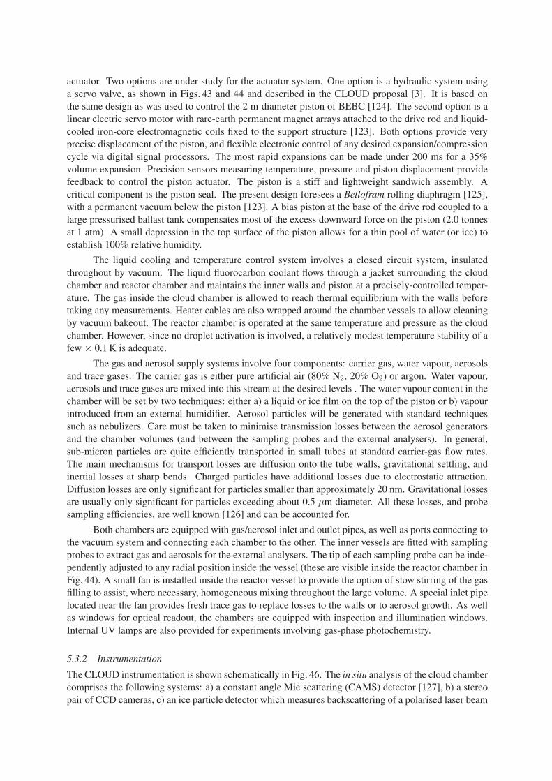
actuator. Two options are under study for the actuator system. One option is a hydraulic system usinga servo valve, as shown in Figs. 43 and 44 and described in the CLOUD proposal [3]. It is based onthe same design as was used to control the 2 m-diameter piston of BEBC [124]. The second option is alinear electric servo motor with rare-earth permanent magnet arrays attached to the drive rod and liquid-cooled iron-core electromagnetic coils fixed to the support structure [123]. Both options provide veryprecise displacement of the piston, and flexible electronic control of any desired expansion/compressioncycle via digital signal processors. The most rapid expansions can be made under 200 ms for a 35%volume expansion. Precision sensors measuring temperature, pressure and piston displacement providefeedback to control the piston actuator. The piston is a stiff and lightweight sandwich assembly. Acritical component is the piston seal. The present design foresees a Bellofram rolling diaphragm [125],with a permanent vacuum below the piston [123]. A bias piston at the base of the drive rod coupled to alarge pressurised ballast tank compensates most of the excess downward force on the piston (2.0 tonnesat 1 atm). A small depression in the top surface of the piston allows for a thin pool of water (or ice) toestablish 100% relative humidity.

The liquid cooling and temperature control system involves a closed circuit system, insulatedthroughout by vacuum. The liquid fluorocarbon coolant flows through a jacket surrounding the cloudchamber and reactor chamber and maintains the inner walls and piston at a precisely-controlled temper-ature. The gas inside the cloud chamber is allowed to reach thermal equilibrium with the walls beforetaking any measurements. Heater cables are also wrapped around the chamber vessels to allow cleaningby vacuum bakeout. The reactor chamber is operated at the same temperature and pressure as the cloudchamber. However, since no droplet activation is involved, a relatively modest temperature stability of afew × 0.1 K is adequate.

The gas and aerosol supply systems involve four components: carrier gas, water vapour, aerosolsand trace gases. The carrier gas is either pure artificial air (80% N2, 20% O2) or argon. Water vapour,aerosols and trace gases are mixed into this stream at the desired levels . The water vapour content in thechamber will be set by two techniques: either a) a liquid or ice film on the top of the piston or b) vapourintroduced from an external humidifier. Aerosol particles will be generated with standard techniquessuch as nebulizers. Care must be taken to minimise transmission losses between the aerosol generatorsand the chamber volumes (and between the sampling probes and the external analysers). In general,sub-micron particles are quite efficiently transported in small tubes at standard carrier-gas flow rates.The main mechanisms for transport losses are diffusion onto the tube walls, gravitational settling, andinertial losses at sharp bends. Charged particles have additional losses due to electrostatic attraction.Diffusion losses are only significant for particles smaller than approximately 20 nm. Gravitational lossesare usually only significant for particles exceeding about 0.5 µm diameter. All these losses, and probesampling efficiencies, are well known [126] and can be accounted for.

Both chambers are equipped with gas/aerosol inlet and outlet pipes, as well as ports connecting tothe vacuum system and connecting each chamber to the other. The inner vessels are fitted with samplingprobes to extract gas and aerosols for the external analysers. The tip of each sampling probe can be inde-pendently adjusted to any radial position inside the vessel (these are visible inside the reactor chamber inFig. 44). A small fan is installed inside the reactor vessel to provide the option of slow stirring of the gasfilling to assist, where necessary, homogeneous mixing throughout the large volume. A special inlet pipelocated near the fan provides fresh trace gas to replace losses to the walls or to aerosol growth. As wellas windows for optical readout, the chambers are equipped with inspection and illumination windows.Internal UV lamps are also provided for experiments involving gas-phase photochemistry.

5.3.2 Instrumentation

The CLOUD instrumentation is shown schematically in Fig. 46. The in situ analysis of the cloud chambercomprises the following systems: a) a constant angle Mie scattering (CAMS) detector [127], b) a stereopair of CCD cameras, c) an ice particle detector which measures backscattering of a polarised laser beam

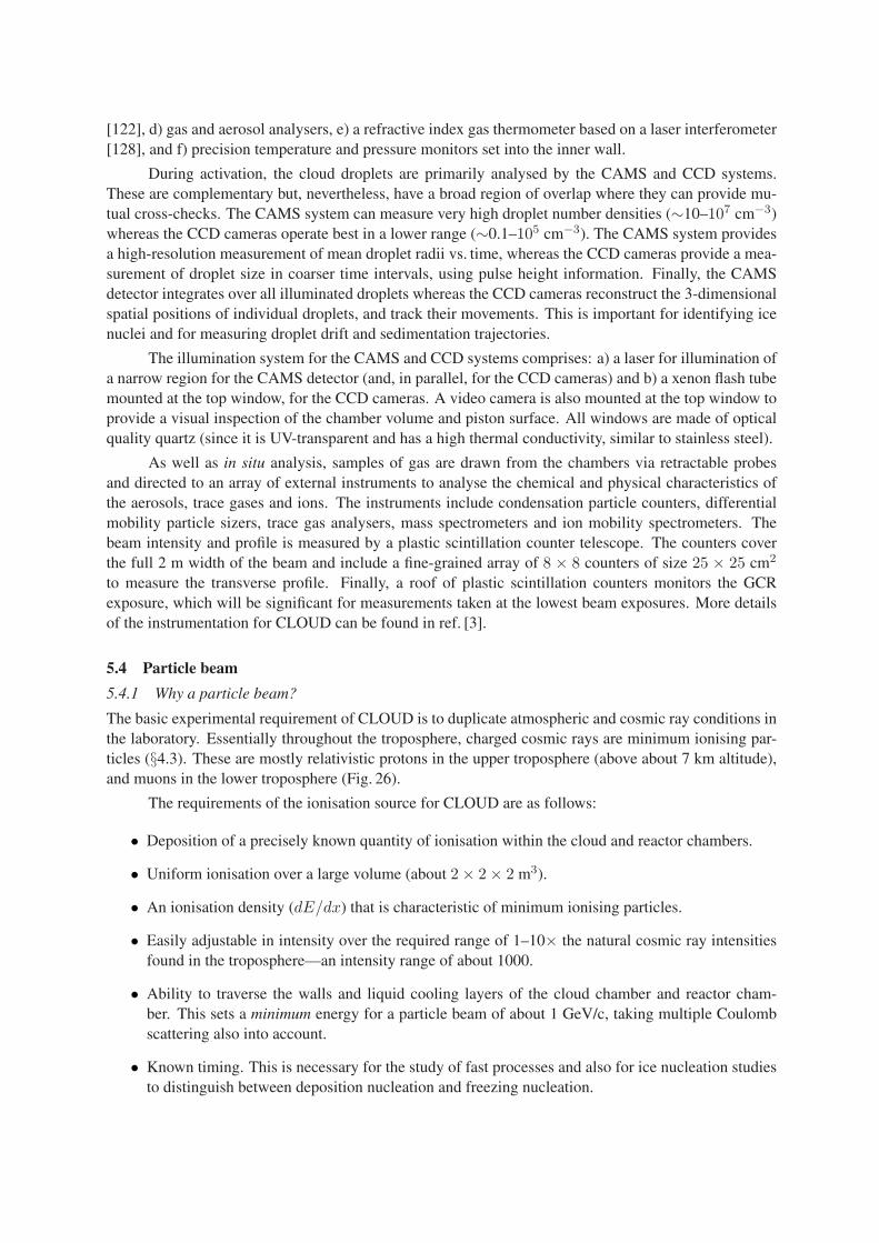
[122], d) gas and aerosol analysers, e) a refractive index gas thermometer based on a laser interferometer[128], and f) precision temperature and pressure monitors set into the inner wall.

During activation, the cloud droplets are primarily analysed by the CAMS and CCD systems.These are complementary but, nevertheless, have a broad region of overlap where they can provide mu-tual cross-checks. The CAMS system can measure very high droplet number densities (∼10–107 cm−3)whereas the CCD cameras operate best in a lower range (∼0.1–105 cm−3). The CAMS system providesa high-resolution measurement of mean droplet radii vs. time, whereas the CCD cameras provide a mea-surement of droplet size in coarser time intervals, using pulse height information. Finally, the CAMSdetector integrates over all illuminated droplets whereas the CCD cameras reconstruct the 3-dimensionalspatial positions of individual droplets, and track their movements. This is important for identifying icenuclei and for measuring droplet drift and sedimentation trajectories.

The illumination system for the CAMS and CCD systems comprises: a) a laser for illumination ofa narrow region for the CAMS detector (and, in parallel, for the CCD cameras) and b) a xenon flash tubemounted at the top window, for the CCD cameras. A video camera is also mounted at the top window toprovide a visual inspection of the chamber volume and piston surface. All windows are made of opticalquality quartz (since it is UV-transparent and has a high thermal conductivity, similar to stainless steel).

As well as in situ analysis, samples of gas are drawn from the chambers via retractable probesand directed to an array of external instruments to analyse the chemical and physical characteristics ofthe aerosols, trace gases and ions. The instruments include condensation particle counters, differentialmobility particle sizers, trace gas analysers, mass spectrometers and ion mobility spectrometers. Thebeam intensity and profile is measured by a plastic scintillation counter telescope. The counters coverthe full 2 m width of the beam and include a fine-grained array of 8 × 8 counters of size 25 × 25 cm2

to measure the transverse profile. Finally, a roof of plastic scintillation counters monitors the GCRexposure, which will be significant for measurements taken at the lowest beam exposures. More detailsof the instrumentation for CLOUD can be found in ref. [3].

5.4 Particle beam

5.4.1 Why a particle beam?

The basic experimental requirement of CLOUD is to duplicate atmospheric and cosmic ray conditions inthe laboratory. Essentially throughout the troposphere, charged cosmic rays are minimum ionising par-ticles (§4.3). These are mostly relativistic protons in the upper troposphere (above about 7 km altitude),and muons in the lower troposphere (Fig. 26).

The requirements of the ionisation source for CLOUD are as follows:

• Deposition of a precisely known quantity of ionisation within the cloud and reactor chambers.

• Uniform ionisation over a large volume (about 2 × 2 × 2 m3).

• An ionisation density (dE/dx) that is characteristic of minimum ionising particles.

• Easily adjustable in intensity over the required range of 1–10× the natural cosmic ray intensitiesfound in the troposphere—an intensity range of about 1000.

• Ability to traverse the walls and liquid cooling layers of the cloud chamber and reactor cham-ber. This sets a minimum energy for a particle beam of about 1 GeV/c, taking multiple Coulombscattering also into account.

• Known timing. This is necessary for the study of fast processes and also for ice nucleation studiesto distinguish between deposition nucleation and freezing nucleation.

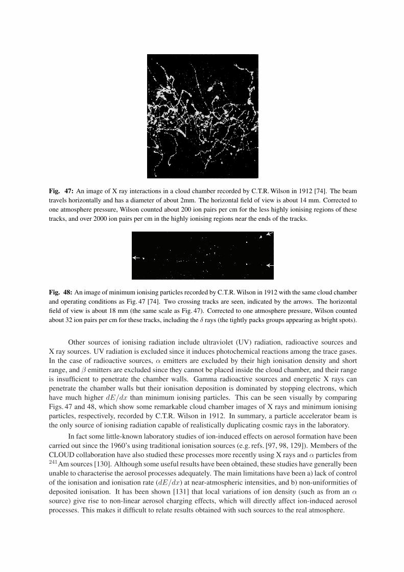
Fig. 47: An image of X ray interactions in a cloud chamber recorded by C.T.R. Wilson in 1912 [74]. The beamtravels horizontally and has a diameter of about 2mm. The horizontal field of view is about 14 mm. Corrected toone atmosphere pressure, Wilson counted about 200 ion pairs per cm for the less highly ionising regions of thesetracks, and over 2000 ion pairs per cm in the highly ionising regions near the ends of the tracks.

Fig. 48: An image of minimum ionising particles recorded by C.T.R. Wilson in 1912 with the same cloud chamberand operating conditions as Fig. 47 [74]. Two crossing tracks are seen, indicated by the arrows. The horizontalfield of view is about 18 mm (the same scale as Fig. 47). Corrected to one atmosphere pressure, Wilson countedabout 32 ion pairs per cm for these tracks, including the δ rays (the tightly packs groups appearing as bright spots).

Other sources of ionising radiation include ultraviolet (UV) radiation, radioactive sources andX ray sources. UV radiation is excluded since it induces photochemical reactions among the trace gases.In the case of radioactive sources, α emitters are excluded by their high ionisation density and shortrange, and β emitters are excluded since they cannot be placed inside the cloud chamber, and their rangeis insufficient to penetrate the chamber walls. Gamma radioactive sources and energetic X rays canpenetrate the chamber walls but their ionisation deposition is dominated by stopping electrons, whichhave much higher dE/dx than minimum ionising particles. This can be seen visually by comparingFigs. 47 and 48, which show some remarkable cloud chamber images of X rays and minimum ionisingparticles, respectively, recorded by C.T.R. Wilson in 1912. In summary, a particle accelerator beam isthe only source of ionising radiation capable of realistically duplicating cosmic rays in the laboratory.

In fact some little-known laboratory studies of ion-induced effects on aerosol formation have beencarried out since the 1960’s using traditional ionisation sources (e.g. refs. [97, 98, 129]). Members of theCLOUD collaboration have also studied these processes more recently using X rays and α particles from241Am sources [130]. Although some useful results have been obtained, these studies have generally beenunable to characterise the aerosol processes adequately. The main limitations have been a) lack of controlof the ionisation and ionisation rate (dE/dx) at near-atmospheric intensities, and b) non-uniformities ofdeposited ionisation. It has been shown [131] that local variations of ion density (such as from an αsource) give rise to non-linear aerosol charging effects, which will directly affect ion-induced aerosolprocesses. This makes it difficult to relate results obtained with such sources to the real atmosphere.

Table 4: Summary of the approximate minimum and maximum time-averaged beam intensities for CLOUD. TheGCR intensity at ground level is about 0.02 cm−ss−1, which is included in column 3 of the table. A transversebeam size of 200 × 200 cm2 is assumed. IGCR signifies the natural GCR intensity at the indicated altitude.

Beam intensity Beam + GCR intensity Clearing Simulated GCR conditions

(s−1) (cm−2s−1) (cm−2s−1) field intensity altitude (km)

0 0 0.02 on 0.01 × IGCR 00 0 0.02 off 1 × IGCR 0

103 0.02 0.04 ” 2 × IGCR 0104 0.2 0.22 ” 10 × IGCR 0

0 0 0.02 ” 0.01 × IGCR 20105 2 2 ” 1 × IGCR 20106 20 20 ” 10 × IGCR 20

5.4.2 Beam requirements

The beam requirements for CLOUD are as follows:

• A muon beam; the ideal particles are µ’s since they replicate the GCR’s in the lower troposphere,and do not interact in the detector material, as would π’s or p’s (e’s are excluded due to showering).

• A mean energy of several GeV, to avoid large multiple Coulomb scattering. The energy spreadshould be known (to calculate the ionisation energy deposition, dE/dx), but it can be broad.

• An adjustable, time-averaged intensity from about 103 s−1 to 106 s−1 (and also zero beam).

• Precise (few per cent) knowledge of the beam intensity (since the solar modulation corresponds toa rather small change of GCR intensity of only ∼10%).

• A large transverse size, 200 × 200 cm2.

• Continual operation throughout the year. A typical single experimental study will require about 4weeks beam-time, and many experiments are foreseen (§5.5).

The desired beam intensity is between about 1× and 10× the natural GCR flux at any altitude.This will allow measurements of the dependence of any observed effects on ionisation rate and ion pairconcentration at the natural ionisation rates in the atmosphere. The highest beam intensities will help toamplify and expose effects before they are measured at natural ionisation levels. Beam-off data will bealso be recorded under conditions with the chamber clearing fields on and off, respectively, correspondingto 0.01× and 1× the natural GCR ion-pair concentrations at ground level.

CLOUD will measure processes over the full range of tropospheric and stratospheric conditions.At ground level, the average GCR intensity is about 0.02 cm−2s−1, whereas at 15–20 km altitude itis about a factor 100 larger, varying between about 0.8 and 2.3 cm−2s−1 depending on geomagneticlatitude (Fig. 27a). The maximum required time-averaged beam intensity is therefore about 10 × 2 =20 cm−2s−1. The beam is spread over a large transverse area of 200 × 200 cm2 in order to duplicate thequasi-uniform GCR irradiation, over the fiducial volume. The time-averaged maximum beam intensityis then 20 × 4 · 104 106 s−1. The minimum beam intensity (apart from beam-off) is about 1× thenatural GCR radiation at ground level. This is a factor 1000 below the maximum required intensity (afactor 100 for the atmospheric attenuation and a factor 10 for 1× the GCR intensity rather than 10×),i.e. a time-averaged intensity of 103 s−1. These beam estimates are summarised in Table 4.

5.5 Experimental programme overview

5.5.1 Aerosol experiments

Gas-to-particle conversion: The aim is to measure the effect of ionising particle radiation on theformation rate of ultrafine condensation nuclei (UCN) in the few-nm size range from trace precursorvapours. Such trace gases include, in particular, H2SO4, HNO3, NH3 and certain volatile organic com-pounds, all in the presence of H2O vapour. The basic parameter to be measured is the UCN nucleationrate, J (cm−3s−1), as a function of the primary experimental variables: trace vapour concentration, rel-ative humidity, temperature, background aerosol concentration and ion-pair production rate. The cloudchamber can measure J over a wide range from about 3 · 10−5 cm−3s−1 to 107 cm−3s−1. Theoreticalstudies [84, 85] indicate that large differences are expected in the ion-induced nucleation rate betweenpositive and negative charges, by factors of up to 100 or more. These effects will be studied either witha ‘saddle’ electric field. Typical formation times (i.e. beam exposures) for these experiments of up toabout one hour are expected.

Growth of CN into CCN: The purpose of these experiments is to measure the effect of ionising particleradiation on the rate of growth of CN into CCN (i.e. from ∼5 nm diameter to ∼100 nm) in the presenceof condensable vapours that are known to be important in the atmosphere, such as sulphuric acid, water,ammonia and organic compounds. Both ‘dry’ and aqueous-phase growth will be studied. The latter willinvolve expansion and compression cycles of the cloud chamber to activate droplets and then evaporatethem. The basic parameter to be measured is the CCN concentration, CCN(S). A progressive expansionwill be used to provide a gradually-increasing supersaturation so that the CCN concentration can bemeasured as a function of S. The CCN are the subset of the CN population that activate into droplets ata given water vapour supersaturation, S. The fraction of the CN that constitute CCN depends not onlyon their size but also on their chemical composition and other properties. The evolution of the CN sizespectra during beam exposure will also be measured. A typical single run will last up to about 2 days.

Activation of CCN into cloud droplets: The goals of these experiments are to see how the presenceof electrical charge affects the critical supersaturations required to activate CCN, and also how it affectsthe number of cloud droplets that appear. Well-defined aerosol sizes will be produced with standardaerosol generation techniques. Experiments will be performed to examine the activation of these aerosolsinto cloud droplets. The charge distribution on the aerosols will be measured in situ using the fieldcage, and externally with the ion mobility spectrometer. A wide range of CCN and ambient conditions(background aerosol, trace gases and thermodynamic conditions) will be explored. The simplest systemswill involve typical hygroscopic aerosols found in the atmosphere, e.g. NaCl, (NH4)2SO4 and H2SO4,and also partially soluble aerosols such as CaSO4. Other measurements will be made on hydrophobiccarbonaceous particles, with and without the presence of organic surfactants. The aims here are toinvestigate the effect of ionisation on the reduction of the critical supersaturations and on the increases ofdroplet number associated with the effects of surface charges [132] and surface tension suppression [54].Finally, these measurements will be repeated in the presence of additional, highly-soluble, trace gases,which are expected to have an extremely low critical supersaturation, even to the point of activating intocloud droplets at below 100% relative humidity [133].

Dynamics of CCN activation and kinetic limitations on cloud droplets: The purpose of these ex-periments is to study the number of droplets that activate from a given CCN population under variousdynamical supersaturation conditions. The calculation of the number of cloud droplets that will activatefrom a given CCN concentration is generally calculated under the assumption the classical Kohler theory(§4.4.1). However this assumes an equilibrium situation whereas, in real clouds, aerosol growth beforeactivation may be kinetically limited [134]. The result can be large errors in the calculated number of

cloud droplets. Since the radiative forcing of clouds is very sensitive to droplet number (§4.4.2), it is im-portant to be able to determine the concentration of cloud droplets to a few per cent. These experimentswill first involve the preparation of a known, polydisperse, CCN population, with various CCN concen-trations and compositions. The number of droplets that activate from these different CCN populationswill then be investigated in the cloud chamber under different realistic adiabatic lapse rates, simulatedby the appropriate progressive expansion cycles, both with and without beam ionisation.

Production of NO and OH and their influence on aerosols: These experiments will first quantifythe poorly-known production rates of a) nitric oxide (NO) and b) hydroxyl radicals (OH) by cosmicrays. Both are important reactive chemicals in the atmosphere and, in certain regions, production byGCRs may be a significant, or perhaps the dominant, mechanism. Estimates made over twenty yearsago [68, 69] suggest about 1–2 OH radicals and 1.5 NO molecules are produced per ion pair. Theseproduction rates would imply maximum mixing ratios of around 1 pptv per day. The production of NOwill be measured in pure artificial air and the production of OH will be measured in argon and watervapour. In a second step, the effect of GCR-produced NO and OH on aerosol nucleation, growth andactivation will be studied by comparing measurements taken with two different carrier gases: artificialair and argon.

Production of aerosol precursors from trace gases: The aim of these experiments is to quantify theinfluence of ionising radiation on various rate-limited chemical reactions that are important for atmo-spheric production of aerosol precursors. For example, sulphuric acid vapour is among the most impor-tant aerosol precursor gases for CCN production. It is mainly produced by oxidation of SO2, which inturn may be emitted directly or else as a product of DMS oxidation (Fig. 35). However the oxidation ofSO2 in the atmosphere is slow since it proceeds by interaction with the rare hydroxyl radical. The lifetimeof SO2 by the OH reaction is about 1 week at typical OH concentrations (105 − 106 molecules cm−3).In contrast, the lifetime of SO2 by dry and wet deposition is about a day. Any process that apprecia-bly increases the rate of SO2 oxidation will therefore increase the H2SO4 concentration. Since GCRsproduce OH radicals, they can in principle influence this reaction. There is in fact some experimental ev-idence that ionising particles may indeed enhance the rate of H2SO4 formation [82]. These experimentswill involve exposing various atmospheric concentrations of trace gases under different thermodynamicconditions to a range of beam fluxes, and then analysing the reaction products.

Effect of highly ionising particles: Although the majority of cosmic rays in the lower troposphere(below about 6 km) are muons, a few per cent are protons. These undergo nuclear reactions, generatinghighly ionising nuclear fragments. The fraction of strongly interacting particles (p, n, π± and heavyions) increases at higher altitudes. It is therefore important to investigate the effect of highly ionisingfragments on the nucleation of aerosols (and perhaps on other processes summarised here) [135]. Theseexperiments will involve the introduction of small amounts of radon gas into the chamber gas mixtures.Radon isotopes are α emitters, e.g. 222Rn decays to 220Po and a 5.5 MeV α, with a 3.8 d half life. Theα particle range in air is about 5 cm at stp, corresponding to an ionisation density, dE/dx, that is abouta factor 500 larger than it is for muons (minimum ionising particles). The data taken with Rn irradiationwill be compared with beam data to study the effects of high ionisation densities.

5.5.2 Ice particle experiments

Ice particle formation by deposition nucleation: The aim is to study the influence of ionisation on theability of aerosols to act as ice nuclei (IN) on which water vapour can be directly sublimated to the solidphase (Fig. 38a). The cloud chamber will be filled with selected aerosols and exposed to the beam. Thebeam is then turned off and expansions made to a range of final temperatures between 0C and -40C.

The efficiency of these aerosols to act directly as IN will be measured as a function of temperature andaerosol charge (using the electric field created by the field cage). The presence of an ice crystal in a cloudof drops is readily identified by the CCD cameras since an ice crystal scatters much more light than awater drop [103]. The ice fraction will also be measured with a backscattered polarised laser beam.

Ice particle formation by freezing nucleation and contact nucleation: These experiments will in-vestigate the influence of ionising radiation on the formation of ice particles via the intermediate stageof supercooled liquid droplets. The expansion chamber will be used to create a supercooled cloud by ex-pansion and growth of droplets at temperatures between 0C and -40C. The temperature of the dropletscan be controlled by the expansion ratio and the initial temperature of the chamber before expansion.After forming the droplets, they are exposed to the beam and the freezing rate is measured. There areseveral ways to disentangle freezing nucleation (Fig. 38b) from contact nucleation (Fig. 38c). The timedevelopment will be different for the two processes (contact nucleation is slower since it is controlledby diffusion of low-mobility aerosols and by sedimentation) and, in addition, CCN that do not act asIN can be included to provide the condensation nucleus for the supercooled droplets. It is important toobserve the freezing process over an extended time. This can be achieved by dynamically adjusting theexpansion piston so that the supercooled droplets neither evaporate nor grow so large that they are lostby sedimentation.

Secondary production of ice particles: These experiments will study the effect of charge on the pro-duction of secondary ice particles by shattering and splintering of freezing droplets. Mixed-phase cloudswill be created at various temperatures and the particles grown to sizes where sedimentation and colli-sions take place. The secondary production of ice particles by contact freezing will be studied. Thesemeasurements will use the CCD cameras to follow the evolution of individual particles and their interac-tions with other particles.

Efficiency of highly-charged evaporation nuclei as IN: These experiments will study the Tinsleymechanism (§4.5.2). This will first involve forming cloud droplets at an appropriate temperature in therange from 0C to -40C, in the presence of selected initial aerosols and trace vapours, including both sol-uble and insoluble (organic) compounds. The droplets will be charged to relatively high values, ∼ 100e,using the beam and electric field. The droplets will then be evaporated by an adiabatic compression, andthe cycle repeated. In this way the effectiveness as IN will be investigated of highly charged aerosolscoated with cloud-processed material.

Effect of freezing-thawing cycles on IN efficiency: These experiments will study the effect of freezing-thawing cycles on the efficiency with which various aerosols act as IN. After filling the cloud chamberwith the aerosols under study, a series of expansion/compression cycles will be used to activate droplets,allow some to form ice particles, and then evaporate them and repeat the cycle.

Growth of ice particles in mixed-phase clouds: The aims of these experiments are to measure thedynamics and ice-particle growth rates in clouds formed of co-existing liquid and ice particles. Clouds atvarious temperatures between 0C and -40C will be generated containing liquid particles and a few iceparticles. The latter will be created using efficient IN such as AgI, in the appropriate low ratios relativeto the CCN (10−4 − 10−6).

Reflectivities of ice and liquid clouds: The aim here is to measure optical reflectivities (albedo) of iceclouds and liquid clouds as functions of water content and particle number concentrations.

Freezing mechanism of polar stratospheric clouds: The aim of these experiments is to investigatethe deposition freezing nucleation of HNO3 and water vapours onto ion clusters, forming nitric acidhydrates. Particles composed of such hydrates are the principal component of the polar stratosphericclouds that initiate the destruction of ozone. The operating temperatures are typical polar stratosphericvalues of between 190 and 200 K. Nitric acid and water vapour will be present the chamber at partialpressures representative of the stratosphere (10−4 Pa for HNO3 vapour and 5 · 10−2 Pa for H2O vapour,corresponding to about 10 ppb and 5 ppm, respectively). At these pressures and temperatures the nitricacid hydrates become supersaturated and can condense as crystals provided a suitable ice nucleus ispresent. Sulphuric acid vapour will be included in the air mixture to represent the species most likely tocontribute to the initial ion cluster formation.

5.5.3 Cloud electricity experiments

Effect of charge and electric field on the coalescence efficiency of droplets: The aim of these ex-periments is to study the effect of charge and electric field on the efficiency with which cloud dropletscoalesce on colliding. Laboratory studies [136] have indicated that raindrops (of around 0.5 mm diame-ter) are about a factor 100 more efficient at collecting aerosol when they are charged rather than neutral,and theoretical studies support this picture [105]. Since collisional growth is the main mechanism bywhich cloud droplets grow into raindrops, this is an important process for determining the lifetime of acloud. These experiments will involve generation of polydisperse droplet distribution in the cloud cham-ber (from a broad initial CCN distribution). The coalescence efficiency will be measured for individualdroplets using the CCD camera system, as a function of droplet size, charge and electric field. In addi-tion, special runs will be taken with high ionisation depositions to simulate the ion densities that mayoccur in thunderstorm conditions, where the coalescence efficiencies may be greatly enhanced.

Charge separation mechanism in clouds: The aim of these experiments is to investigate whetherthere are any differences in critical supersaturation between positively and negatively charged CCN.Theoretical studies [112] suggest that negative particles may activate more readily than positive particles.If this occurs under natural cloud conditions then it could lead to charge separation, the precursor forlightning. In these experiments the beam will first ionise the cloud chamber volume and the chargeallowed to be scavenged by a predetermined CCN population. The beam will be turned off and theclearing field used to separate the positive and negative charged aerosols. A progressive piston expansionwill gradually raise the supersaturation. The activation of the positively-charged CCN region can then becompared with the negatively-charged CCN region. After activation, the charges on the aerosols can bemeasured by further drifting in an electric field set with the field cage. The activations will be measuredas functions of the CCN type, beam intensity, aerosol charge, electric field and adiabatic lapse rate (rateof rise of supersaturation).

Lightning trigger mechanism: The aim here is to investigate the proposed triggering mechanism forlightning due to high energy primary cosmic rays [113]. The charge amplification in the cores of theseshowers will be studied under typical cloud conditions (i.e. cloud droplets and electric fields). A singlepulse of about 2 · 104 beam particles over a 2 × 2 m2 area simulates the peak electron shower densityin the core of 1015 eV primary GCR. Higher particle densities can easily be generated. The field cagegenerates electric fields of up to 10 kVm−1, which will simulate the fields in all but lightning clouds.Higher fields typical of lightning breakdown conditions (100 kVm−1) can be generated using speciallydesigned electrodes inserted into the chamber via the sampling probes. For these experiments an X raydetector will be used to observe possible X ray emissions from avalanche processes.

Effect of electrical discharge on cloud droplet formation: The aim of these experiments is to studythe effects of electrical discharges on cloud droplet number and on droplet coalescence efficiency, andespecially to quantify the effects of NOx production from electrical discharges. Since GCRs may influ-ence the rate of lightning, they may in turn influence this important source of NOx in the atmosphere. Itis interesting to note that cloud chamber experiments in Edinburgh in the 1960’s observed backgroundsdue to ‘hypersensitive condensation nuclei’ [137]. These activated into droplets at very low water vapoursupersaturations—of order 1%—and were attributed to trace amounts of NO2 vapour created by electro-static discharges. As before, the discharges will be generated by specially designed electrodes insertedinto the cloud chamber via the sampling probes.

5.5.4 Data interpretation and cloud modelling

The experimental results obtained with CLOUD will be evaluated with aerosol and cloud simulations.The basic physics aims of these simulations are as follows:

1. To incorporate the microphysics of ion-mediated processes into the aerosol and cloud models.

2. To examine the sensitivity of clouds under atmospheric conditions to variations in the GCR inten-sity, in the presence of other sources of natural variability.

There will be a close feedback between the simulations and the experimental observations toconfirm a) that the simulations closely reproduce the experimental data and b) that the underlying micro-physics is understood. The simulations will also eventually become important in guiding the direction ofthe experimental programme.

As well as a detector simulation, this work will require a complete simulation of the microphysicalprocesses under study. Already existing within the CLOUD collaboration are detailed models of aerosolnucleation, growth and activation, and also two sophisticated cloud models—for cumulus and marinestratus clouds, respectively. Ion-mediated microphysics will be incorporated into these models based onthe experimental data from CLOUD. If item 2 above reveals discernible GCR effects on single clouds,suitable parametrisations will be prepared for the climate modelling community to explore the influenceof GCR effects on the global climate.

6 CONCLUSIONS

The Sun is a variable star. The sunspot record over the last 400 years reveals both a quasi-periodicsolar cycle of about 11 years and also longer-term changes, including a grand minimum lasting about70 years during which the sunspots all but disappeared. This coincided with the most pronounced ofseveral prolonged cold spells between 1450 and 1890 which are collectively known as the Little Ice Age.Light radio-isotope records in ice cores, tree rings and other archives extend the measurements of solarvariability back over the last 250 kyr. They reveal numerous occasions when the Sun waxed or wanedover centennial periods.

The Earth’s climate is far from stable. Natural forcings have caused large climate changes in thepast. The most important are the periodic shifts from glacial epochs lasting about 100 kyr to warminter-glacial epochs lasting about 10 kyr. These transitions involve global average temperature changesof about 5C, and polar changes of 10–15C. They coincide with the Milankovitch orbital variationsof the Earth around the Sun, but amplification mechanisms are needed to account for the magnitude ofthe observed climate changes. However, in addition to these large climate shifts, recent palaeoclimaticstudies have shown that significant climate variations also occurred within the Holocene and the lastice age on centennial and millennial timescales. There is increasing evidence that many of these aretriggered by solar forcing. It appears that the Little Ice Age was but one of around 10 solar-induced coldspells during the last 10,000 years.

However, despite the extensive evidence, solar variability remains a controversial agent of climatechange since no causal mechanism has been established to link the two phenomena. Estimates of thevariation of the solar irradiance appear to be too small to account for the observed climate variability.Until recently there were no indications where else to look. However, recent satellite data have provideda new clue: low cloud cover may be influenced by the Sun—either as a result of changes in the elec-tromagnetic (UV) radiation or in the galactic cosmic rays, whose flux is modulated by the solar wind.This could provide an effective initial step by which an energetically-weak solar signal is amplified intoa significant climate forcing. Subsequently, in response to the cloud radiative and hydrological changes,further amplification processes may occur such as shifts of the global thermohaline system, which canexert major global climatic effects.

The cosmic ray hypothesis for solar-climate variability rests on the microphysical interactions ofcosmic rays and clouds, which are experimentally poorly-known. The CLOUD experiment proposesa major investigation of ion-aerosol-cloud microphysics under controlled laboratory conditions using abeam from a particle accelerator, which provides a precisely adjustable and measurable artificial sourceof cosmic rays. The heart of the experiment is a precision cloud chamber that recreates cloud conditionsthroughout the atmosphere. CLOUD is designed as a flexible, general purpose detector, and a broad rangeof measurements of cloud microphysics is planned in the areas of aerosols, ice particles and atmosphericelectricity. Unique in the world, this facility would open up an essentially new line of atmosphericresearch. Its primary task is to pursue the question of how cosmic rays may influence clouds. If cloudsrespond to the solar variations that modulate the cosmic rays reaching the Earth, there are consequencesfor the evaluation of climate change, since the 20th century warming coincided with a large increase ofsolar activity. To settle the issue, one way or the other, is therefore of great importance.

Finally, since this paper begins with a quote, it is perhaps fitting to end with another [138]:

The physics of cloud formation appears in every aspect of the climate variation, includ-ing direct heating by sunlight. I would hope that with the important issues that need to bedecided in connection with climate variation and global warming, an all out effort can belaunched to understand this vital aspect of atmospheric science. There is a lot of laboratorywork to be done under carefully controlled conditions, e.g. the CERN [CLOUD] experi-ment, on the nucleation of aerosols, ice crystals, and water drops, as well as the relatedfield work to study the application of the laboratory results.. . .Our ability to handle the scientific challenge of climate change will be a subject of futurehistorical research and writing. The eyes of future generations will be upon us. There hasnever been an individual scientific problem that will have so much impact as the globalwarming inquiry on the long term well being of the human race.

Eugene N. Parker, University of ChicagoConference Summary, The Solar Cycle and Terrestrial Climate

Santa Cruz de Tenerife, September 2000

Acknowledgements

It is a pleasure to thank Jurg Beer, Gordon Bowden, Nigel Calder, Maurice Jacob, Lew Keller, Ralph Nel-son, David Ritson, Arnold Wolfendale and my CLOUD collaborators for many interesting and enjoyablediscussions.

References

[1] H. Svensmark and E. Friis-Christensen, Variation in cosmic ray flux and global cloud coverage—amissing link in solar-climate relationships, Journal of Atmospheric and Solar-Terrestrial Physics59 (1997) 1225.

[2] N. Marsh and H. Svensmark, Low cloud properties influenced by solar activity,http://arXiv.org/abs/physics/000507, Phys. Rev. Lett. 85 (2000) 5004–5007.

[3] CLOUD collaboration (B. Fastrup et al.), A study of the link between cosmic rays and cloudswith a cloud chamber at the CERN PS, http://www.cern.ch/cloud/iaci workshop/cloud.html, CERNproposal SPSC/P317, SPSC 2000-021 (2000).

[4] CLOUD collaboration (B. Fastrup et al.), Addendum to the CLOUD proposal,http://www.cern.ch/cloud/iaci workshop/cloud.html, CERN SPSC/P317 Add.1, SPSC 2000-030 (2000).

[5] CLOUD collaboration (B. Fastrup et al.), CLOUD: an Atmospheric Research Facility at CERN,http://www.cern.ch/cloud/iaci workshop/cloud.html, CERN SPSC/P317 Add.2, SPSC 2000-041(2000).

[6] J.M. Wilcox, Solar activity and the weather, J. Atm. & Sol.-Terr. Phys. 37 (1975) 237–256.

[7] W. Herschel, Observations tending to investigate the nature of the Sun, in order to find out thecauses or symptoms of its variable emission of light and heat, Philosophical Transactions of theRoyal Society, London (1801) 265.

[8] J.A. Eddy, The Maunder minimum, Science 192 (1976) 1189.

[9] C. Frohlich and J. Lean, The Sun’s total irradiance: Cycles and trends in the past two decades andassociated climate change uncertainties, Geophys. Res. Lett. 25 (1998) 4377–4380.

[10] J. Lean, J. Beer and R.S. Bradley, Reconstruction of solar irradiance since 1610: Implications forclimate change, Geophys. Res. Lett. 22 (1995) 3195–3198.

[11] M. Lockwood, R. Stamper and M.N. Wild, A doubling of the Sun’s coronal magnetic field duringthe past 100 years, Nature 399 (1999) 437.

[12] S.C. Kernthaler, R. Toumi and J.D. Haigh, Some doubts concerning a link between cosmic rayfluxes and global cloudiness, Geophys. Res. Lett. 26 (1999) 863–865.

[13] T.S. Jorgensen and A.W. Hansen, Journal of Atmospheric and Solar-Terrestrial Physics 62 (1997)73–77. A reply is in the adjacent paper: H. Svensmark and E. Friis-Christensen, Journal of Atmo-spheric and Solar-Terrestrial Physics 62 (1997) 79–80.

[14] J.E. Kristjansson and J. Kristiansen, Is there a cosmic ray signal in recent variations in globalcloudiness and cloud radiative forcing?, J. Geophys. Res. 105 (2000) 11851–11863.

[15] W.B. Rossow, A.W. Walker, D.E. Beuschel, and M.D. Roiter, International Satellite Cloud Clima-tology Project (ISCCP): documentation of new cloud datasets, WMO/TD 737, World Meteorolog-ical Organization, Geneva (1996).

[16] M. Lockwood, Changes in galactic cosmic ray flux, solar irradiance and climate over the past 150years, in Proc. of the Workshop on Ion-Aerosol-Cloud Interactions, ed. J. Kirkby, CERN, Geneva,CERN 2001-007 (2001).

[17] D.V. Hoyt and K.H. Schatten, The Role of the Sun in Climate Change, Oxford University Press,Oxford (1997).

[18] C.E.P. Brooks, Variations in the levels of the central African Lakes Victoria and Albert, GeophysicalMemoirs, London, 2 (1923) 327–334.

[19] G.W. Lockwood and D.T. Thompson, Photometric variability of Neptune, 1972–2000, in press(2001).

[20] N. Marsh and H. Svensmark, GCR and ENSO trends in ISCCP-D2 low cloud properties, submittedto J. Geophys. Res. (2001); also http://www.dsri.dk/∼ndm/CLOUD UPDATE/UPDATE.html.

[21] D.L. Hartmann, Radiative effects of clouds on Earth’s climate, in Aerosol-Cloud-Climate Interac-tions, International Geophysics Series, Vol. 54, ed. P.V. Hobbs, Academic Press Inc., San Diego(1993) 151.

[22] J. Beer, Ice core data on climate and cosmic ray changes, in Proc. of the Workshop on Ion-Aerosol-Cloud Interactions, ed. J. Kirkby, CERN, Geneva, CERN 2001-007 (2001).

[23] J.R. Herman and R.A. Goldberg, Sun, Weather, and Climate, NASA SP 426 (1978).

[24] K.C. Taylor et al., The Holocene-Younger Dryas transition recorded at Summit, Greenland, Science278 (1997) 825.

[25] W.S. Broecker and G.H. Denton, What drives glacial cycles?, Scientific American 262 (1990) 43–50.

[26] B. Stenni et al., An ocean reversal during the last deglaciation, Science 293 (2001) 2074–2077.

[27] J.P. Sachs et al., Glacial surface temperatures of the Southeast Atlantic Ocean, Science 293 (2001)2077–2079.

[28] R. Muscheler, J. Beer, G. Wagner and R.C. Finkel, Changes in deep-water formation during theYounger Dryas event inferred from 10Be and 14C records, Nature 408 (2000) 567–570.

[29] H. Renssen, B. van geel, J. van der Plicht and M. Magny, Reduced solar activity as a trigger for thestart of the Younger Dryas?, Quaternary International 68–71 (2000) 373–383.

[30] G.C. Bond and R. Lotti, Iceberg discharges into the North Atlantic on millennial time scales duringthe last glaciation, Science 267 (1997) 1005–1010.

[31] G.C. Bond et al., A pervasive millennial-scale cycle in North Atlantic Holocene and glacial cli-mates, Science 278 (1997) 1257-1266.

[32] A. Ganopolski and S. Rahmstorf, Rapid changes of glacial climate simulated in a coupled climatemodel, Nature 409 (2001) 153–158.

[33] G. Wagner, C. Laj, J. Beer et al., Reconstruction of the paleo accumulation rate of central Greenlandduring the last 75 kyr using the cosmogenic radionuclides 36Cl and 10Be, and geomagnetic fieldintensity data, in press (2001).

[34] G.C. Bond, B. Kromer, J. Beer, R. Muscheler, M.N. Evans, W. Showers, S. Hoffmann, R. Lotti-Bond, I. Hajdas and G. Bonani, Persistant solar influence on North Atlantic climate during theHolocene, Science 294 (2001) 2130–2136.

[35] M. Magny, Lake level fluctuations in the Jura and French subalpine regions associated with ice-rafting in the North Atlantic and variations in the polar atmospheric circulation, Quaternaire 10(1999) 61–64.

[36] U. Neff et al., Strong coincidence between solar variability and the monsoon in Oman between 9and 6 kyr ago, Nature 411 (2001) 290–293.

[37] B. van Geel, J. Buurman and H.T. Waterbolk, Archaeological and palaeoecological indicationsof an abrupt climate change in The Netherlands, and evidence for climatological teleconnections,around 2650 BP, J. Quaternary Science 11 (1996) 451–460.

[38] M. Grosjean et al., A late Holocene (<2600 BC) glacial advance in the south-central Andes (29S),northern Chile, The Holocene 8 (1998) 473–479.

[39] V.J. Polyak and Y. Asmerom, Late Holocene climate and cultural changes in the southwesternUnited States, Science 294 (2001) 148–151.

[40] P.E. Damon and C.P. Sonett, Solar and terrestrial components of the atmospheric 14C variationspectrum, in The Sun in Time, eds. C.P. Sonett, M.S. Giampapa and M.S. Matthews, University ofArizona Press, Tucson (1991) 360.

[41] G.A. Brook et al., The Holocene 9 (1999) 695.

[42] R.F. Denniston et al., Quat. Res. 53 (2000) 196.

[43] D. Verschuren, K. Laird and B. Cumming, Rainfall and drought in equatorial East Africa duringthe past 1100 years, Nature 403 (2000) 410–414.

[44] G. Cini Castagnoli et al., The role of cloud cover on the solar illumination signal recorded by δ13Cof a shallow water Ionian Sea core, in Proc. of the Workshop on Ion-Aerosol-Cloud Interactions,ed. J. Kirkby, CERN, Geneva, CERN 2001-007 (2001).

[45] J. Beer, S. Tobias and N. Weiss, An active Sun throughout the Maunder Minimum, Solar Physics181 (1998) 237–249.

[46] J. Beer, A. Blinov, G. Bonani, H.J. Hofmann and R.C. Finkel, Use of 10Be in polar ice to trace the11-year cycle of solar activity, Nature 347 (1990) 164–166.

[47] M. Lockwood, J. Geophys. Res. 106 (2001) 16021–16038.

[48] T. Landscheidt, Solar forcing of El Nino and La Nina, in Proc. of the First Solar & Space WeatherEuroconference; The Solar Cycle and Terrestrial Climate, Santa Cruz de Tenerife, Spain, ESASP-463 (2000) 2135–2140.

[49] Climate Change 2001: The Scientific Basis, Intergovernmental Panel on Climate Change, eds.J.T. Houghton et al., Cambridge University Press, UK (2001).

[50] G.C. Reid, Influence of solar variability on global sea surface temperatures, Nature 329 (1987)142–143.

[51] D. Ritson, private communication.

[52] W.B. White, J. Lean, D.R. Cayan and M.D. Dettinger, Response of global upper ocean temperatureto changing solar irradiance, J. Geophys. Res. 102 C2 (1997) 3255-3266.

[53] W.B. White, D.R. Cayan and J. Lean, Global upper ocean heat storage response to radiative forcingfrom changing solar irradiance and increasing greenhouse gas/aerosol concentrations, J. Geophys.Res. 103 C10 (1998) 21,333–21,366.

[54] R.J. Charlson, J.H. Seinfeld, A. Nenes, M. Kulmala, A. Laaksonen and M. Christina Facchini,Reshaping the theory of cloud formation, Science 292 (2001) 2025–2026.

[55] Y.I. Stozhkov, N.S. Svirzhevsky and V.S. Makhmutov, Cosmic ray measurements in the atmo-sphere, in Proc. of the Workshop on Ion-Aerosol-Cloud Interactions, ed. J. Kirkby, CERN, Geneva,CERN 2001-007 (2001).

[56] Y.C. Unruh, S.K. Solanki and M. Fligge, Modelling solar irradiance variations: comparisonwith observations, including line-ratio variations, in Solar Variability and Climate, eds. E. Friis-Christensen et al., Space Science Reviews 94, Nos. 1–2 (2000) 145–152.

[57] J.D. Haigh, The impact of solar variability on climate, Science 272 (1996) 981.

[58] D. Shindell et al., Solar cycle variability, ozone, and climate, Science 284 (1999) 305–308.

[59] K.J.H. Phillips, Guide to the Sun, Cambridge University Press, UK (1992).

[60] N.O. Weiss and S.M. Tobias, Physical causes of solar activity, in Solar Variability and Climate,eds. E. Friis-Christensen et al., Space Science Reviews 94, Nos. 1–2 (2000) 99–112.

[61] J. Schou et al., Helioseismic studies of differential rotation in the solar envelope by the Solar Oscil-lation Investigation using the Michelson Doppler Imager, Astrophysical Journal 505 (1998) 390–417.

[62] E.N. Parker, The passage of energetic charged particles through interplanetary space, Planet. SpaceSc. 13 (1965) 9–49.

[63] L.J. Gleeson and W.I. Axford, Cosmic rays in the interplanetary medium, Astrophys. Journal 149(1967) 1115–1118.

[64] D.E. Groom et al. (Particle Data Group), The Review of Particle Physics, The European PhysicalJournal C15 (2000) 150–156.

[65] V.I. Ermakov, G.A. Bazilevskaya, P.E. Pokrevsky and Y.I. Stozhkov, Ion balance equation in theatmosphere, J. Geophys. Res. 102 (1997) 23413.

[66] S. Tonwar (private communication, based on data from the L3+C experiment at CERN).

[67] P.J. Crutzen and F. Arnold, Nitric acid formation in the cold antarctic atmosphere: a major causefor the springtime ‘ozone hole’, Nature 324 (1986) 651.

[68] M. Nicolet, On the production of nitric oxide by cosmic rays in the mesosphere and stratosphere,Planet. Space Sci. 23 (1975) 637.

[69] C.H. Jackman, J.E. Frederick and R.S. Stolarski, Production of odd nitrogen in the stratosphere andmesosphere: an intercomparison of signal strengths, J. Geophys. Res. 85 C12 (1980) 7495.

[70] P.J. Crutzen, I.A.S. Isaksen and G.C. Reid, Solar proton events: stratospheric sources of nitricoxide, Science 189 (1975) 457.

[71] A.A. Viggiano and F. Arnold, Ion chemistry and composition of the atmosphere, Handbook ofAtmospheric Electrodynamics, Vol. 1, ed. H. Volland, CRC Press, Boca Raton (1998).

[72] H. Heitmann and F. Arnold, Composition measurements of tropospheric ions, Nature 306 (1993)747.

[73] A. Krieger and F. Arnold, First composition measurements of stratospheric negative ions and in-ferred gaseous sulphuric acid in the winter arctic vortex: Implications for aerosols and hydroxylradical formation, Geophys. Res. Lett. 21 (1994) 1259.

[74] C.T.R. Wilson, Expansion apparatus, Proc. Royal Society of London A 87 (1912) 277.

[75] J.H. Seinfeld and S.N. Pandis, Atmospheric Chemistry and Physics, Wiley, New York (1998).

[76] S. Twomey, Aerosols, clouds, and radiation, Atmos. Environ. 25A (1991) 2435–2442.

[77] P.V. Hobbs, Aerosol-cloud interactions, in Aerosol-Cloud-Climate Interactions, International Geo-physics Series, Vol. 54, ed. P.V. Hobbs, Academic Press Inc., San Diego (1993) 33–73.

[78] S.E. Schwartz and A. Slingo, Enhanced shortwave cloud radiative forcing due to anthropogenicaerosols, in Clouds, Chemistry and Climate, Proceedings of NATO Advanced Study Workshop, ed.P. Crutzen and V. Ramanathan, Springer, Heidelberg (1996) 191–236.

[79] L.F. Radke, J.A. Coakley and M.D. King, Science 246 (1989) 1146–1149.

[80] D. Rosenfeld, Suppression of rain and snow by urban and industrial air pollution, Science 287(2000) 1793.

[81] F. Arnold, Multi-ion complexes in the stratosphere: implications for trace gases and aerosols, Na-ture 284 (1980) 610.

[82] F. Raes and A. Janssens, Ion-induced aerosol formation in a H2O-H2SO4 system - I. Extension ofthe classical theory and search for experimental evidence, J. Aerosol Sci. 16 (1985) 217.

[83] F. Raes, A. Janssens and R.V. Dingenen, The role of ion-induced aerosol formation in the loweratmosphere, J. Aerosol Sc. 17 (1986) 466.

[84] I. Kusaka, Z.G. Wang and J.H. Seinfeld, Ion-induced nucleation: a density functional approach, J.Chem. Phys. 102 (1995) 913–924.

[85] I. Kusaka, Z.G. Wang and J.H. Seinfeld, Ion-induced nucleation. II. Polarizable multipolarmolecules, J. Chem. Phys. 103 (1995) 8993–9009.

[86] R.P. Turco, J.-K. Zhao and F. Yu, A new source of tropospheric aerosols: ion-ion recombination,Geophys. Res. Lett. 25 (1998) 635.

[87] F. Yu and R.P. Turco, Ultrafine aerosol formation via ion-mediated nucleation, Geophys. Res. Lett.27 (2000) 883.

[88] M. Kulmala, Atmospheric aerosols: formation and growth, in Proc. of the Workshop on Ion-Aerosol-Cloud Interactions, ed. J. Kirkby, CERN, Geneva, CERN 2001-007 (2001).

[89] A.D. Clarke et al., Particle nucleation in the tropical boundary layer and its coupling to marinesulfur sources, Science 282 (1998) 89.

[90] R.J. Weber et al., Measurement of new particle formation and ultrafine particle growth at a cleancontinental site, J. Geophys. Res. 102 (1997) 4375–4385.

[91] R.J. Weber et al., New particle formation in the remote troposphere: a comparison of observationsat various sites, Geophys. Res. Lett. 26 (1999) 307–310.

[92] M.K. Kulmala, L. Pirjola and J.M. Makela, Stable sulphate clusters as a source of new atmosphericparticles, Nature 404 (2000) 66.

[93] F. Yu and R.P. Turco, From molecular clusters to nanoparticles: The role of ambient ionisation intropospheric aerosol formation, J. Geophys. Res. 106 (2001) 4797–4814.

[94] R. D’Auria and R.P. Turco, A thermodynamic-kinetic model for ionic cluster formation, growthand nucleation, Proc. of the Workshop on Ion-Aerosol-Cloud Interactions, ed. J. Kirkby, CERN,Geneva, CERN 2001-007 (2001).

[95] F. Yu, Cosmic rays, particle formation, natural variability of global cloudiness, and climate impli-cations, in Proc. of the Workshop on Ion-Aerosol-Cloud Interactions, ed. J. Kirkby, CERN, Geneva,CERN 2001-007 (2001).

[96] U. Horrak, J. Salm and H. Tammet, Bursts of intermediate ions in atmospheric air, J. GeophysicalResearch 103 D12 (1998) 13909.

[97] J. Bricard et al., Formation and evolution of nuclei of condensation that appear in air initially freeof aerosols, J. Geophysical Research 73 (1968) 4487.

[98] K.G. Vohra, M.C. Subba Ramu and T.S. Muraleedharan, An experimental study of the role ofradon and its daughter products in the conversion of sulphur dioxide into aerosol particles in theatmosphere, Atmospheric Environment 18 (1984) 1653.

[99] B. Zuberi et al., Heterogeneous freezing of aqueous particles induced by crystallized (NH4)2SO4,ice, and letovicite, J. Physical Chemistry A 105 (2001) 6458–6464.

[100] B.A. Tinsley and G.W. Dean, Apparent tropospheric response to MeV–GeV particle flux varia-tions: a connection via the solar wind, atmospheric electricity and cloud microphysics, J. Geophys-ical Research 96 (1991) 22283.

[101] B.A. Tinsley, Influence of solar wind on the global electric circuit, and inferred effects on cloudmicrophysics, temperature, and dynamics in the troposphere, in Solar Variability and Climate, eds.E. Friis-Christensen et al., Space Science Reviews 94, Nos. 1–2 (2000) 231–258.

[102] H.R. Pruppacher and J.D. Klett, Microphysics of Clouds and Precipitation, 2nd ed., Kluwer Aca-demic Publishers, The Netherlands (1997).

[103] R.J. Anderson, R.C. Miller, J.L. Kassner and D.E. Hagen, A study of homogeneous condensation-freezing nucleation of small water droplets in an expansion cloud chamber, J. Atmospheric Sciences37, No. 11 (1980) 2508–2520.

[104] A.E. Waibel, T. Peter, K.S. Carslaw, H. Oelhaf, G. Wetzel, P.J. Crutzen, U. Poschl, A. Tsias, E.Reimer and H. Fischer, Arctic ozone loss due to denitrification, Science 283 (1999) 2064–2069.

[105] D.R. MacGorman and W.D. Rust, The Electrical Nature of Storms, Oxford University Press, UK(1998).

[106] K. Schlegel et al., Thunderstorms, lightning and solar activity—Middle Europe, J. Atmosphericand Solar-Terrestrial Physics, 63 (2001) 1705–1713.

[107] R.G. Roble, On solar-terrestrial relationships in the atmospheric electricity, J. Geophys. Res. 90(1985) 6000.

[108] R.E. Orville and G.R. Huffines, Lightning ground flash measurements over the contiguous UnitedStates: a ten-year summary 1989–1998, in Proc. 11th Int. Conf. on Atmospheric Electricity, Al-abama, USA (1999) 412.

[109] B.J. Kellett, The production of atmospheric nitric oxide by cosmic rays and solar energetic par-ticles, in Proc. of the Workshop on Ion-Aerosol-Cloud Interactions, ed. J. Kirkby, CERN, Geneva,CERN 2001-007 (2001).

[110] Yu. I. Stozhkov et al., Rainfalls during great Forbush decreases, Il Nuovo Cimento 18C (1995)335.

[111] M.I. Pudovkin and S.V. Veretenenko, Cloudiness decreases associated with Forbush decreases ofgalactic cosmic rays, J. Atmos. Solar-Terrestrial Phys. 75 (1995) 1349.

[112] A.I. Rusanov and F.M. Kuni, Reformulation of the thermodynamic theory of nucleation oncharged particles, J. Colloid and Interface Science 100 (1984) 264.

[113] A.V. Gurevich, K.P. Zybin and R. Roussel-Dupre, Lightning initiation by simultaneous effect ofrunaway breakdown and cosmic ray showers, Phys. Lett. A 254 (1999) 79–87.

[114] A.P. Chubenko et al., Intensive X-ray emission bursts during thunderstorms, Phys. Lett. A 275(2000) 90–100.

[115] C.B. Moore, K.B. Eack, G.D. Aulich and W. Rison, Energetic radiation associated with lightningstepped-leaders, Geophys. Res. Lett. 28 No. 11 (2001) 2141–2144.

[116] P. Galison, Image and Logic; a Material Culture of Microphysics, University of Chicago Press,Chicago (1997).

[117] A. Nenes, P.Y. Chuang, R.C. Flagan and J.H. Seinfeld, A theoretical analysis of cloud condensa-tion nucleus (CCN) instruments, J. Geophys. Res. 106 D4 (2001) 3449–3474.

[118] P.E. Wagner, Experiments on nucleation processes in aerosols, in Proc. of the Workshop on Ion-Aerosol-Cloud Interactions, ed. J. Kirkby, CERN, Geneva, CERN 2001-007 (2001).

[119] J.L. Schmitt, Comments on the operation of a Wilson expansion cloud chamber, in Proc. ofthe Workshop on Ion-Aerosol-Cloud Interactions, ed. J. Kirkby, CERN, Geneva, CERN 2001-007(2001).

[120] N.N. Das Gupta and S.K. Ghosh, A report on the Wilson cloud chamber and its application inphysics, Rev. Modern Physics 18 (1946) 225–290.

[121] H. Bunz et al., The novel aerosol chamber facility AIDA: status and first results, in Proc. 7th Eu-ropean Symposium on the Physico-Chemical Behaviour of Atmospheric Pollutants, eds. B. Larson,B. Versino and G. Angeletti, Venice (1996) 673.

[122] O. Mohler et al., The Karlsruhe aerosol chamber facility AIDA: Technical description and firstresults of homogeneous and heterogeneous ice nucleation experiments, in Proc. of the Workshopon Ion-Aerosol-Cloud Interactions, ed. J. Kirkby, CERN, Geneva, CERN 2001-007 (2001).

[123] G.B. Bowden, private communication.

[124] A. Herve and G. Bachy, Huge electrohydraulic servovalves control 2-ton cryogenic piston, Hy-draulics & Pneumatics, Pention/IPC, Cleveland, Ohio (1977); and, The hydraulic expansion servo-system of the Big European Bubble Chamber, CERN preprint CERN/EF 77-6 (1977).

[125] Bellofram Corporation, Burlington, MA 01803, USA, http://www.marshbellowfram.com.

[126] W.C. Hinds, Aerosol Technology: Properties, Behavior, and Measurement of Airborne Particles,John Wiley & Sons, Inc., New York (1998).

[127] P.E. Wagner, A constant-angle Mie scattering method (CAMS) for investigation of particle forma-tion processes, J. Colloid Interface Sci. 105 (1985) 456.

[128] F. Pavese and G. Molinar, Modern Gas-Based Temperature and Pressure Measurements, The In-ternational Cryogenics Monograph Series, Plenum Press, New York (1992).

[129] T.P. Burke and J.A. Scott, The production of condensation nuclei by alpha radiation, Proc. RoyalIrish Academy 73 A (1973) 151–158.

[130] J.M. Makela, Studies on irradiation induced aerosol particle formation processes in air containingsulphur dioxide, Ph.D. thesis, Univ. Helsinki, Acta Polytechnica Scandinavica, Applied PhysicsSeries 82 (1992).

[131] C.F. Clement and R.G. Harrison, Enhanced localised charging of radioactive aerosols, J. Aerosol.Sci. 31, 3 (2000) 363–378.

[132] A.S. Wexler and Z. Ge, Hydrophobic particles can activate at lower relative humidity than slightlyhygroscopic ones: a Kohler theory incorporating surface fixed charge, J. Geophys. Res. 103 D6(1998) 6083–6088.

[133] M. Kulmala, A. Laaksonen, R.J. Charlson and P. Korhonen, Clouds without supersaturation, Na-ture 388 (1997) 336.

[134] P.Y. Chuang, R.J. Charlson and J.H. Seinfeld, Kinetic limitations on droplet formation in clouds,Nature 390 (1997) 594–596.

[135] A.D. Erlykin and A.W. Wolfendale, Cosmic rays and the Earth’s atmosphere, in Proc. of the Work-shop on Ion-Aerosol-Cloud Interactions, ed. J. Kirkby, CERN, Geneva, CERN 2001-007 (2001).

[136] A.K. Barlow and J. Latham, A laboratory study of the scavenging of sub-micron aerosol bycharged raindrops, Quart. J. R. Met. Soc. 109 (1983) 763–770.

[137] G.R. Evans and A.A. Watson, Production of hypersensitive condensation nuclei, Nature 196(1962) 729; G.R. Evans et al., Some remarks on the origin and elimination of background cloudin expansion cloud chambers, J. Sci. Inst. 41 (1964) 770; G.R. Evans and A.A. Watson, Nitrogendioxide vapour and the creation of condensation nuclei, Proc. Royal Society of Edinburgh LXVIIpart III-10 (1966) 136.

[138] E.N. Parker, Summary and perspectives, in Proc. of the First Solar & Space Weather Euroconfer-ence; The Solar Cycle and Terrestrial Climate, Santa Cruz de Tenerife, Spain, ESA SP-463 (2000)263–269.

CONCLUSIONS OF THE WORKSHOP ON ION-AEROSOL-CLOUDINTERACTIONS, CERN, 18-20 APRIL 2001

A.W. WolfendaleDepartment of Physics, University of Durham, South Road, Durham, DH1 3LE, U.K.

AbstractRecent observations suggest that cosmic rays may play a significant role inthe climate. In particular, satellite data have revealed a surprising correlationbetween cosmic ray intensity and the fraction of the Earth covered by lowclouds. Since the cosmic ray intensity is modulated by the solar wind, thiscould provide an important clue to the long-sought mechanism connectingsolar and climate variability. Moreover, if this connection were to beestablished, it could have significant consequences for our understanding ofthe solar contributions to the present global warming, since the cosmic rayintensity has fallen during the 20th century due to a more-than-doubling ofthe strength of the solar wind. In order to the test whether cosmic rays and clouds are causally linked and, ifso, to understand the microphysical mechanisms, a novel experiment knownas CLOUD has been proposed at CERN by an interdisciplinary collaborationof atmospheric, solar-terrestrial, cosmic ray and particle physicists. CLOUDproposes to use a CERN pion beam as an artificial source of cosmic rays.The beam would pass through an expansion cloud chamber in which theatmospheric conditions within clouds throughout the atmosphere could bereproduced. All parameters of the experiment would be precisely controlledand measured.A workshop was recently held at CERN to discuss the scientific case for aconnection between cosmic rays and clouds, and to review the proposedCLOUD facility. The outcome was a clear consensus that the scientificindications of a cosmic ray-cloud link are both interesting and important,and that plausible microphysical mechanisms exist but their significance isnot yet known. There was unanimous agreement on the urgent need toperform controlled laboratory measurements to test the cosmic ray-cloudlink in a particle beam at CERN, as proposed by the CLOUD experiment.Further details on the outcome of the workshop are provided below.

1. INTRODUCTION

The European Geophysical Society, the European Physical Society and the European ScienceFoundation co-sponsored an inter-disciplinary "Workshop on Ion-Aerosol-Cloud Interactions" atCERN, 18-20 April 2001. The workshop was attended by about 50 physicists representing 14countries and drawn from the atmospheric, aerosol, palaeoclimatological, solar-terrestrial, cosmic rayand particle physics communities. This aim of the meeting was twofold:

1) To review the present knowledge of ion-aerosol-cloud interactions and their possible role in solar-climate variability.

2) To review the proposed CLOUD Atmospheric Research Facility using a particle beam at CERN.

2. PROCEDURE

In order to arrive at a consensus on the workshop conclusions, the meeting closed with a "WorkshopSummary Panel" discussion. The panel members comprised:

Sir Arnold Wolfendale /University of Durham (chairman)

Maurice Jacob /Chairman of the Joint Astrophysics Division of EAS and EPS

Mike Lockwood /RAL, President of Solar-Terrestrial Sciences, EGS

Richard Turco /University of California, Los Angeles

Paul Wagner /University of Vienna

To focus the discussion, the chairman presented four basic (but inevitably over-simplified)questions to the panel and then to the floor:

1) "Does cosmic ray ionization play a role in the climate?"

2) "Is the mechanism: ionization -> aerosol -> cloud understood?"

3) "Is the case (scientific motivation) for a cosmic ray influence on cloud cover agreed?"

4) "Would the CERN 'CLOUD' facility satisfy a need?"

As well as a general discussion, the chairman invited all those present (numbering about 30 inthe final session) to vote either "No", "?" or "Yes" to each question. Finally, after each question hadbeen discussed and voted in turn, the chairman invited the panel and floor to express their opinionson a fifth question:

5) "Why at CERN?"

The points raised during the discussion on each question are summarised below, together withthe results of the voting.

3. RESPONSES TO THE QUESTIONS

3.1 "Does cosmic ray ionization play a role in the climate?"

Elaboration: This question asked whether cosmic rays have the potential to affect the climate andwhether there is evidence that it may be happening. The question did not ask whether cosmic rays doindeed significantly affect the climate - which is clearly unanswerable at present.

Discussion: Clear historical correlations of sunspot/solar variability and changes in the Earth's climatewere presented at the workshop. For example, Beer, Lockwood and van Geel showed examples suchas the Maunder Minimum (Little Ice Age), the circa-850BC climate anomaly and the Younger Dryascold event at the end of the last Ice Age (12.9-11.6 kyear before present) which are associated withsolar variability as revealed in the sunspot record and in the cosmogenic isotope record in ice-cores(10Be) and tree-rings (14C). These data directly indicate the prevailing galactic cosmic ray (GCR)intensities, which are modulated by the solar wind (and by slower changes in the Earth's magneticdipole). However the solar/GCR-climate correlations are sometimes present and sometimes not. Thismay reflect the complexity of the Earth's climate - that many factors are important and they interactin a complex way. The climate may have stable states such that a correlation may persist for somedecades and then disappear for a while. In addition, whatever caused those earlier natural climateshifts may also be interacting with today's anthropogenic contributions in the atmosphere to produce

a yet more complex response, for example anthropogenic sulphur dioxide and its effect on cloudcover.

However, correlations do not demonstrate cause and effect, so the present data are unable toseparate whether the Sun-Earth coupling is via electromagnetic radiation (total irradiance/UV/...)and/or via energetic cosmic rays (galactic/solar). But it is important to note that these are the onlypossible vectors (it is unlikely that the solar wind itself could be directly responsible) - and so at leastone of them must be implicated. In the case of cosmic rays one should in particular study andunderstand the amplification factors that would be necessary to enhance their role despite their verysmall energy input (roughly equivalent to that of starlight) in comparison with total solar irradiance.(The vast disparity of energies, by itself, does not exclude the possibility of an effect; there arenumerous examples in physics of large energy amplification factors, such as a nuclear chain reactionreleased by a few initial neutrons.)

In the case of the current global warming, there is increasing agreement that the climate modelfits to the temperature record need to amplify the solar contribution by about a factor 3. Thepresently-assumed solar contribution is only from the (Lean et al., 1995) direct irradiance changes.An additional, indirect, solar contribution could either decrease or increase the projections of theanthropogenic effects. (The latter possibility arises since an increased solar attribution during the lastcentury could indicate a steeper anthropogenic rise in recent decades.)

The satellite data analysis presented at the workshop by Svensmark indicates a solar cyclecorrelation with low cloud cover, suggesting that the solar-climate mechanism may involve clouds.Again, at this stage both electromagnetic radiation and GCRs remain as candidates. This may providethe first clue to the long-sought amplification mechanism linking solar and climate variability.However the underlying processes may involve subtleties since the observed solar correlation isconfined to low clouds, and the global correlation map of low cloud cover shows no preference forhigh geomagnetic latitudes - both of which appear to be counter-intuitive at first sight.

Vote: The distribution of votes on the question "Does cosmic ray ionization play a role in theclimate?" was equally divided between "?" and "Yes", with zero votes for "No". This implies that thereare reasonable indications that cosmic rays have the potential to affect the climate but that thequestion of whether they are significant is far from settled.

3.2 "Is the mechanism: ionization -> aerosol -> cloud understood?"

Elaboration: This question asked whether there is any microphysical understanding of themechanism(s) by which cosmic ray ionization could affect 1) the nucleation of new aerosol and 2) thelifetime, albedo or other properties of clouds.

Discussion: There is now strong evidence to support the existence of the first step. Yu and Turcopresented the results of their theoretical studies of ion-induced nucleation and conclude that ions playan important role in the creation and early growth of ultrafine condensation nuclei (UCN) from tracevapours such as sulphuric acid. These frequently occur in clean environments (such as over oceans)at very low concentrations where classical nucleation theory predicts no nucleation should occur - butnevertheless nucleation is observed. Yu and Turco find that that the presence of charge serves tostabilise the embryonic clusters, and their ion-mediated model agrees with the experimentalobservations. In addition, Yu reported on the effect of variations of GCR ionization at differentaltitudes and concludes that it can be the limiting factor to aerosol nucleation at low altitudes, whereasat high altitudes, where the ionization rate is up to a factor 20 larger, other parameters such the trace

gas concentrations become the limiting factor. This would provide a possible explanation why thesolar modulation is observed only in low clouds.

As well as theoretical developments, F.Arnold presented at the workshop the first directobservation of ion-induced nucleation in the laboratory, and also aircraft measurements of the ionmass spectrum in the atmosphere which extend to large ions and indicate the presence of ion-inducednucleation.

These theoretical and experimental developments represent significant progress and lay to resta common criticism raised against the cosmic ray-cloud hypothesis - namely that no microphysicalmechanism exists to connect cosmic rays to clouds. At least one mechanism exists but whether or notit is significant is not yet known. Whereas there now seems little doubt that cosmic rays can influencethe nucleation of trace condensable vapours under certain conditions, the effect of these extra UCNon the cloud condensation nuclei (CCN) that seed cloud droplets is an open question. Equally, theinfluence of GCRs on the growth process of other aerosols or on the activation of CCN into droplets isnot known. However, if cosmic rays could indeed modify the CCN number concentration in certainregions of the atmosphere then this may affect both cloud lifetimes and albedo. Furthermore, GCRsmay have other effects on clouds such as the electrofreezing of supercooled liquid droplets,influences on the global electrical circuit and electric field strength, and the production of tracereactive chemicals (NO, OH) which could affect atmospheric chemistry at certain altitudes. Insummary, there are now actually several mechanisms that have been identified by which GCRs maypotentially affect clouds, but they are yet to be investigated experimentally and quantified.

Vote: The distribution of votes on the question "Is the mechanism: ionization -> aerosol -> cloudunderstood?" was bimodal. There was a 100% "Yes" vote for the first step, indicating that at least onemechanism is explicable theoretically, if not proven experimentally (although the first directobservations of ion-induced aerosol formation were presented at the workshop). However whether ornot these UCN have a significant effect on CCN is essentially unknown. This was reflected in the votefor the second step which was equally divided between "No" and "?", with zero votes for "Yes". Thislatter vote indicates also the poor experimental and theoretical understanding of the effects ofionization on the aerosol growth and activation processes, and on other areas where it may play a role.

3.3 "Is the case (scientific motivation) for a cosmic ray influence on cloud cover agreed?"

Elaboration: This question asked whether the scientific indications are sufficiently interesting andimportant to merit a controlled laboratory experiment on the influence of cosmic rays on clouds.

Discussion: In view of the preceding discussion on the first two questions, there was little extradiscussion before a vote was taken on this third question. However it was pointed out that the GCR-cloud hypothesis may be the very first hard clue we have as to what is behind the solar-climatecorrelations that have been observed over the last two centuries. If our only tool is correlations, wemay continue another two centuries and still not be able to understand the underlying mechanism.However at last we have a definite hypothesis that can be tested experimentally: "Are cosmic raysaffecting cloud formation?". The question is so important that we should pursue it.

Vote: On the question "Is the case (scientific motivation) for a cosmic ray influence on cloud coveragreed?": 100% "Yes".

3.4 "Would the CERN 'CLOUD' facility satisfy a need?"

Elaboration: This question asked whether the CERN 'CLOUD' facility would provide important newexperimental data on the subject of ion-aerosol-cloud interactions and whether the facility would becomplementary to other experiments in this field.

Discussion: It was agreed that the CLOUD facility is timely for several reasons. First of course are therecent satellite observations of a solar modulation of cloud cover, and its possible effect on the climateand global warming. Recent theoretical progress has been made on the understanding of ion-mediated effects on aerosols by Yu, Turco, Okuyama and others, and there is now an urgent need forexperimental data to test these models. Finally, it is only in the last few years that the necessaryprecision experimental tools have been developed which will allow the proposed CLOUD experimentsto be carried out.

At the workshop Möhler presented the experience with the Karlsruhe aerosol chamber facility,AIDA, which has successfully demonstrated the feasibility of aerosol growth experiments in thelaboratory under atmospheric conditions. Furthermore Wagner described recent measurements whichshow expansion cloud chambers to be versatile and high-precision experimental tools that are ideallysuited for the proposed studies. With expansion cloud chambers, well-defined thermodynamicconditions can be produced over large volumes and, with the use of a CERN particle beam, the cosmicray conditions throughout the atmosphere can be recreated. The proposed CLOUD facility would bethe world's first to precisely simulate the conditions inside clouds at all altitudes and latitudes, and toinvestigate the effects of ionizing particle radiation on aerosol and cloud processes.

In addition to aerosol nucleation, growth and activation experiments, CLOUD will be able tomeasure the effect of cosmic ray ionization on a wide range of atmospheric processes. For example,Carslaw described at the workshop how ionization has been proposed as the possible mechanism bywhich polar stratospheric clouds freeze. Discovery of the freezing mechanism in these clouds iscrucial to our understanding of de-nitrification and subsequent ozone loss over the poles. Kellettshowed evidence for production of nitric oxide in the atmosphere by energetic solar cosmic rayevents and suggested that GCRs may affect the rate of NO production in the lower atmosphere byaffecting lightning production. Stozhkov in fact presented ground-based data collected in someregions of the United States that shows a correlation between the GCR intensity and the frequency oflightning. Stozhkov also suggested that a preferential activation of water droplets on negative ionsmay be responsible for charge separation in clouds, and therefore lightning. He also presented dataindicating a decreased rainfall during Forbush decreases, and increased rainfall during energetic solarcosmic ray events. GCRs are responsible for the fair weather ionization throughout most of the loweratmosphere and are therefore a key element in the global electrical circuit. Harrison summarisedseveral atmospheric electricity processes, such as electrofreezing, aerosol charging, and the scavengingof charged aerosols by cloud droplets, that may play important roles in cloud microphysics.

The CLOUD facility can investigate the fundamental physics that underlies each of theseprocesses. It would provide important microphysical measurements to help the interpretation ofatmospheric observations by programmes such as the ESF SPECIAL network to study Sun-Earthlinks, which Rycroft described at the meeting. In short, there is not a single "need" for CLOUD but,rather, a wide range of "needs", making the concept of a facility appropriate for the project.Furthermore, CLOUD should be seen as providing an essential and complementary contribution insupport of an extensive on-going solar-terrestrial experimental programme involving satellites andground-based stations.

Vote: On the question "Would the CERN 'CLOUD' facility satisfy a need?": 100% "Yes".

3.5 "Why at CERN?"

Elaboration: This question asked why the CLOUD facility should be located at CERN.

Discussion: There are two basic reasons why CERN is uniquely suitable for the CLOUD facility: a) theparticle beam and b) technological expertise and excellence in the equipment needed for theexperiment, together with rapidly-increasing knowledge by talented staff of the detailed researchproblems to be addressed.

The theoretical studies of Yu, Turco and others have shown that ionization effects are highlynon-linear and so experiments must reproduce ionization rates and ionization densities (dE/dx) closeto natural GCRs. Such measurements have so far never been achieved with radioactive sources despiteexperiments over the last 40 years. However, a CERN pion beam closely duplicates natural GCRs andprovides a precisely controlled and delivered particle ionization inside the active volumes of theexperiment.

To answer the scientific questions addressed by CLOUD requires a sophisticated andtechnically-challenging experimental apparatus - one that is beyond the capabilities of individualinstitutes but well within the scope of the experiments for which CERN is well known. In particularCERN has key expertise in the expansion cloud chamber, from its experience with BEBC and otherbubble chambers. In this sense the CLOUD facility could be considered as a "technology transfer"from CERN, but to another research community rather than to industry, and on a subject of greatinterest to society. The project represents a unique interface that brings together cosmic ray/particlephysics - which is within the mandate of CERN - and atmospheric physics. Such a facility may attractEU funding support. The facility coincides with a research hiatus at CERN over the next 5 yearswhile the LHC is being constructed.

As well as issues related to the beam and technological expertise, the CLOUD facility hasattracted an enthusiastic interdisciplinary collaboration with an unprecedented range of experienceand skills.

However, the prime reasons "Why at CERN?" are the importance of the CLOUD facility toscience and to society; and CERN is the unique European host.

Yes?No

Yes?No

Yes?No

Yes?No

Yes?No

Voting result

1) "Does cosmic ray ionization play a role in the climate?"

2) "Is the mechanism understood for: a) ionization -> aerosol?

and

b) aerosol -> cloud?"

3) "Is the scientific motivation for a cosmic ray influence on cloud cover agreed?"

4) "Would the CERN 'CLOUD' facility satisfy a need?"

Summary of the Conclusions of theWorkshop on Ion-Aerosol-Cloud Interactions,

CERN, 18-20 April 2001

Fig.1 Summary of the voting results at the workshop.