cooperative routing for collision minimization in wireless

Cooperative Routing for Collision Minimization in

Wireless Sensor Networks

by

© Fatemeh Mansourkiaie

A dissertation submitted to the School of Graduate Studies

in partial fulfilment of the requirements for the degree of

Doctor of Philosophy

Faculty of Engineering and Applied Science

Memorial University of Newfoundland

May 2016

St. John’s, Newfoundland

Abstract

Cooperative communication has gained much interest due to its ability to exploit the

broadcasting nature of the wireless medium to mitigate multipath fading. There has

been considerable amount of research on how cooperative transmission can improve the

performance of the network by focusing on the physical layer issues. During the past few

years, the researchers have started to take into consideration cooperative transmission in

routing and there has been a growing interest in designing and evaluating cooperative

routing protocols. Most of the existing cooperative routing algorithms are designed to

reduce the energy consumption; however, packet collision minimization using cooperative

routing has not been addressed yet. This dissertation presents an optimization framework

to minimize collision probability using cooperative routing in wireless sensor networks.

More specifically, we develop a mathematical model and formulate the problem as a

large-scale Mixed Integer Non-Linear Programming problem. We also propose a solution

based on the branch and bound algorithm augmented with reducing the search space

(branch and bound space reduction). The proposed strategy builds up the optimal routes

from each source to the sink node by providing the best set of hops in each route, the best

set of relays, and the optimal power allocation for the cooperative transmission links. To

reduce the computational complexity, we propose two near optimal cooperative routing

algorithms. In the first near optimal algorithm, we solve the problem by decoupling the

optimal power allocation scheme from optimal route selection. Therefore, the problem

ii

is formulated by an Integer Non-Linear Programming, which is solved using a branch

and bound space reduced method. In the second near optimal algorithm, the cooperative

routing problem is solved by decoupling the transmission power and the relay node se-

lection from the route selection. After solving the routing problems, the power allocation

is applied in the selected route. Simulation results show the algorithms can significantly

reduce the collision probability compared with existing cooperative routing schemes.

iii

Acknowledgements

As the formal part of my education comes to an end, it is a great pleasure to acknowledge

several individuals who have had contributed to who I am today.

I would like to offer my sincere thanks to my supervisor Dr. Mohamed H. Ahmed

for his continued and valuable guidance. I greatly appreciate the time he has spent

contributing to this research and to my professional development. Without his guidance

and persistent help this dissertation would not have been possible. The financial support

provided by my supervisor, the Faculty of Engineering and Applied Science, the School

of Graduate Studies is duly acknowledged.

A significant part of my education was in Iran and my foundations were laid in schools

at the city of Tehran. I would like to thank my elementary school teachers, my math

teachers at secondary and high schools, my B.Sc. project supervisor, and my M.Sc.

thesis supervisor.

The final word of acknowledgement is reserved for my parents for their unconditional

support, to my husband for his love, patience and unwavering belief in me, without their

continuous support and encouragement, this dissertation would not have been possible.

iv

Co-Authorship Statements

I, Fatemeh Mansourkiaie, hold a principal author status for all the manuscript chapters

(Chapter 2 - 5) in this dissertation. However, each manuscript is co-authored by my

supervisor, whose contributions have facilitated the development of this work as described

below.

Paper 1 in Chapter 2: Fatemeh Mansourkiaie and Mohamed H. Ahmed, “Coopera-

tive Routing in Wireless Networks: A Comprehensive Survey,” IEEE Communica-

tions Surveys and Tutorials, vol. 17, no. 2, pp 604-626, Apr. 2015.

I was the primary author and with my supervisor contributed to the idea, its for-

mulation and development, and refinement of the presentation.

Paper 2 in Chapter 3: Fatemeh Mansourkiaie and Mohamed H. Ahmed, “Joint

Cooperative Routing and Power Allocation for Collision Minimization in Wireless

Sensor Networks,” submitted to IEEE Wireless Communication and Networking

Conference, Apr. 2016.



Paper 3 in Chapter 4: Fatemeh Mansourkiaie and Mohamed H. Ahmed, “Per-Node

v

Traffic Load in Cooperative Wireless Sensor Networks,” under review, IEEE Com-

munications Letters.



Paper 4 in Chapter 5: Fatemeh Mansourkiaie and Mohamed H. Ahmed, “Joint

Cooperative Routing and Power Allocation for Collision Minimization in Wireless

Sensor Networks with Multiple Flows,” IEEE Wireless Communications Letters,

vol. 4, no. 1, pp. 6-9, Feb. 2015.



Paper 5 in Chapter 6: Fatemeh Mansourkiaie and Mohamed H. Ahmed, “Optimal

and Near-Optimal Cooperative Routing and Power Allocation for Collision Mini-

mization in Wireless Sensor Networks,” under review, IEEE Sensors Journal.



Fatemeh Mansourkiaie Date

vi

Contents

Abstract ii

Acknowledgments iv

Co-Authorship Statements v

Table of Content vii

List of Figures xiii

List of Tables xvi

List of Abbreviations xvii

1 Introduction 1

1.1 Background . . . . . . . . . . . . . . . . . . . . . . . . . . . . . . . . . . . 1

1.2 Research Motivation . . . . . . . . . . . . . . . . . . . . . . . . . . . . . . 5

1.3 Thesis Contribution . . . . . . . . . . . . . . . . . . . . . . . . . . . . . . . 7

1.4 Thesis Outline . . . . . . . . . . . . . . . . . . . . . . . . . . . . . . . . . . 9

REFERENCES . . . . . . . . . . . . . . . . . . . . . . . . . . . . . . . . . 11

vii

2 Cooperative Routing in Wireless Networks: A Comprehensive Survey 14

2.1 Abstract . . . . . . . . . . . . . . . . . . . . . . . . . . . . . . . . . . . . . 14

2.2 Introduction . . . . . . . . . . . . . . . . . . . . . . . . . . . . . . . . . . . 15

2.3 Background of Cooperative Routing . . . . . . . . . . . . . . . . . . . . . . 19

2.3.1 Cooperative Transmission Scheme . . . . . . . . . . . . . . . . . . . 20

2.3.1.1 Relaying Techniques . . . . . . . . . . . . . . . . . . . . . 20

2.3.1.2 Combining Techniques . . . . . . . . . . . . . . . . . . . . 21

2.3.2 Relay Node Selection . . . . . . . . . . . . . . . . . . . . . . . . . . 22

2.3.2.1 Optimal number of relay nodes . . . . . . . . . . . . . . . 23

2.3.2.2 Optimal relay node placement . . . . . . . . . . . . . . . . 23

2.3.3 Resource Allocation in Cooperative Communication . . . . . . . . . 24

2.3.4 Channel State Information (CSI) . . . . . . . . . . . . . . . . . . . 25

2.3.5 Network Coding in Cooperative Diversity . . . . . . . . . . . . . . . 26

2.3.6 Cooperative Routing Metrics . . . . . . . . . . . . . . . . . . . . . 27

2.3.7 Cooperative Routing Applications . . . . . . . . . . . . . . . . . . . 28

2.4 Taxonomy of Cooperative Routing Protocols . . . . . . . . . . . . . . . . . 28

2.4.1 Optimality . . . . . . . . . . . . . . . . . . . . . . . . . . . . . . . . 29

2.4.2 Objective . . . . . . . . . . . . . . . . . . . . . . . . . . . . . . . . 30

2.4.3 Centralization . . . . . . . . . . . . . . . . . . . . . . . . . . . . . . 31

2.5 Cooperative Routing Optimality . . . . . . . . . . . . . . . . . . . . . . . . 31

2.5.1 Optimal Cooperative Routing Schemes . . . . . . . . . . . . . . . . 31

2.5.2 Sub-Optimal Cooperative Routing . . . . . . . . . . . . . . . . . . . 32

2.5.2.1 Cooperative Along Non-cooperative Path . . . . . . . . . 32

2.5.2.2 Cooperative-Based Path . . . . . . . . . . . . . . . . . . . 33

viii

2.6 Cooperative Routing Objectives . . . . . . . . . . . . . . . . . . . . . . . . 36

2.6.1 Energy-Efficient Cooperative Routing . . . . . . . . . . . . . . . . . 36

2.6.1.1 Energy-Efficient Cooperative Link . . . . . . . . . . . . . 38

2.6.1.2 Energy-Efficient Relay Node Assignment . . . . . . . . . . 38

2.6.1.3 Energy Efficient Path Selection . . . . . . . . . . . . . . . 39

2.6.1.4 Combination of The Aforementioned Techniques . . . . . 39

2.6.2 QoS-Aware Cooperative Routing . . . . . . . . . . . . . . . . . . . 39

2.6.3 Minimum Collision Cooperative Routing . . . . . . . . . . . . . . . 42

2.7 Centralization . . . . . . . . . . . . . . . . . . . . . . . . . . . . . . . . . . 43

2.7.1 Centralized Cooperative Routing . . . . . . . . . . . . . . . . . . . 43

2.7.2 Distributed Cooperative Routing . . . . . . . . . . . . . . . . . . . 44

2.8 Overview of Existing Cooperative Routing Algorithms . . . . . . . . . . . 45

2.9 Performance and Challenges of Cooperative Routing . . . . . . . . . . . . . 64

2.9.1 Complexity . . . . . . . . . . . . . . . . . . . . . . . . . . . . . . . 72

2.9.2 Multiple Flows . . . . . . . . . . . . . . . . . . . . . . . . . . . . . 74

2.10 Conclusion and Future Work . . . . . . . . . . . . . . . . . . . . . . . . . . 75

REFERENCES 79

3 Joint Cooperative Routing and Power Allocation for Collision Mini-

mization in Wireless Sensor Networks 94

3.1 Abstract . . . . . . . . . . . . . . . . . . . . . . . . . . . . . . . . . . . . . 94

3.2 Introduction . . . . . . . . . . . . . . . . . . . . . . . . . . . . . . . . . . . 95

3.3 System Model and Problem Formulation . . . . . . . . . . . . . . . . . . . 98

3.4 Power Allocation in Cooperative Transmission Links . . . . . . . . . . . . 104

ix

3.5 Proposed Cooperative Routing for Collision Minimization . . . . . . . . . . 106

3.6 Results . . . . . . . . . . . . . . . . . . . . . . . . . . . . . . . . . . . . . . 108

3.6.1 Evaluation of Routing Algorithms . . . . . . . . . . . . . . . . . . . 110

3.6.2 Effect of Power Allocation . . . . . . . . . . . . . . . . . . . . . . . 112

3.7 Conclusion . . . . . . . . . . . . . . . . . . . . . . . . . . . . . . . . . . . . 113

REFERENCES 115

4 Per-Node Traffic Load in Cooperative Wireless Sensor Networks 118

4.1 abstract . . . . . . . . . . . . . . . . . . . . . . . . . . . . . . . . . . . . . 118

4.2 Introduction . . . . . . . . . . . . . . . . . . . . . . . . . . . . . . . . . . . 119

4.3 System Model . . . . . . . . . . . . . . . . . . . . . . . . . . . . . . . . . . 120

4.4 Analysis of Per-Node Traffic Load in a Cooperative Link . . . . . . . . . . 123

4.4.1 Determining the Forwarding Probability to the Next Node in the

Route (Next Hop) . . . . . . . . . . . . . . . . . . . . . . . . . . . 124

4.4.2 Evaluating the Forwarding Probability to the Relay . . . . . . . . . 127

4.5 Simulation Results . . . . . . . . . . . . . . . . . . . . . . . . . . . . . . . 129

4.6 CONCLUSIONS . . . . . . . . . . . . . . . . . . . . . . . . . . . . . . . . 131

REFERENCES 131

5 Joint Cooperative Routing and Power Allocation for Collision Mini-

mization in Wireless Sensor Networks with Multiple Flows 134

5.1 abstract . . . . . . . . . . . . . . . . . . . . . . . . . . . . . . . . . . . . . 134

5.2 Introduction . . . . . . . . . . . . . . . . . . . . . . . . . . . . . . . . . . . 135

5.3 System Model and Problem Formulation . . . . . . . . . . . . . . . . . . . 137

x

5.4 Power Allocation in Cooperative Transmission Links . . . . . . . . . . . . 142

5.5 Proposed Cooperative Routing for Collision Minimization . . . . . . . . . . 143

5.6 Results . . . . . . . . . . . . . . . . . . . . . . . . . . . . . . . . . . . . . . 145

5.7 Conclusion . . . . . . . . . . . . . . . . . . . . . . . . . . . . . . . . . . . . 147

REFERENCES 148

6 Optimal and Near-Optimal Cooperative Routing and Power Allocation

for Collision Minimization in Wireless Sensor Networks 150

6.1 abstract . . . . . . . . . . . . . . . . . . . . . . . . . . . . . . . . . . . . . 150

6.2 Introduction . . . . . . . . . . . . . . . . . . . . . . . . . . . . . . . . . . . 151

6.3 System Model . . . . . . . . . . . . . . . . . . . . . . . . . . . . . . . . . . 157

6.4 Problem Formulation . . . . . . . . . . . . . . . . . . . . . . . . . . . . . . 159

6.5 Proposed Solution Procedure . . . . . . . . . . . . . . . . . . . . . . . . . . 165

6.5.1 Branch and Bound Space Reduced algorithm . . . . . . . . . . . . . 165

6.5.2 A Lower Bound for The Collision Problem . . . . . . . . . . . . . . 167

6.5.3 Complexity . . . . . . . . . . . . . . . . . . . . . . . . . . . . . . . 169

6.6 Near-optimal Cooperative Routing for Collision Minimization . . . . . . . 170

6.7 Performance Evaluation . . . . . . . . . . . . . . . . . . . . . . . . . . . . 172

6.7.1 Comparison between the proposed collision minimization coopera-

tive routing algorithms . . . . . . . . . . . . . . . . . . . . . . . . . 174

6.7.2 Evaluating the effect of cooperative routing parameters . . . . . . . 176

6.7.3 Comparison between the proposed cooperative routing and mini-

mum power cooperative routing algorithms . . . . . . . . . . . . . . 177

xi

6.7.4 Evaluating the total power consumption, considering retransmission

of collided packets . . . . . . . . . . . . . . . . . . . . . . . . . . . 179

6.8 Conclusion . . . . . . . . . . . . . . . . . . . . . . . . . . . . . . . . . . . . 180

REFERENCES 183

7 Conclusions and Future Work 186

7.1 Introduction . . . . . . . . . . . . . . . . . . . . . . . . . . . . . . . . . . . 186

7.2 Conclusions . . . . . . . . . . . . . . . . . . . . . . . . . . . . . . . . . . . 186

7.3 Future Work . . . . . . . . . . . . . . . . . . . . . . . . . . . . . . . . . . . 191

REFERENCES 194

xii

List of Figures

1.1 Cooperative Communication . . . . . . . . . . . . . . . . . . . . . . . . . . 3

2.1 Cooperative Communication. . . . . . . . . . . . . . . . . . . . . . . . . . 16

2.2 A sample cooperative route: Constructing the route using Cooperative

Transmission (CT) and Direct Transmission (DT). . . . . . . . . . . . . . . 20

2.3 Taxonomy of Cooperative Routing. . . . . . . . . . . . . . . . . . . . . . . 29

2.4 The potential relay nodes are located in the intersection area of the coverage

circle. . . . . . . . . . . . . . . . . . . . . . . . . . . . . . . . . . . . . . . 34

2.5 Route chosen by the CAN-L algorithm in a grid wireless network [42]. . . . 47

2.6 Vehicles and roadside units in vehicular networks [67]. . . . . . . . . . . . . 51

2.7 Illustration of EBCR to pick the helper set for current node vi which will

send the same packet simultaneously to next hop node vi+1. The large

circle represents neighborhood N (vi) of vi and the small circle represents

one of the potential cooperative helper sets H (vi) of vi [70]. . . . . . . . . 52

2.8 Route chosen by the MPCR algorithm in a grid wireless network [34]. . . . 54

2.9 Virtual Node and Virtual Link in CCR [64]. . . . . . . . . . . . . . . . . . 56

2.10 Wireless mesh network of base stations [37]. . . . . . . . . . . . . . . . . . 58

2.11 Optimal distance in PACR when l = 1 [37]. . . . . . . . . . . . . . . . . . . 59

xiii

2.12 Non-cooperative and cooperative links as building blocks for a route from

S (source node) to D (destination node). R is selected as a relay node

for the cooperative link, and Sr is the communication range. The shadow

region is the intersected communication area of A and D [72]. . . . . . . . 62

2.13 Routing performance versus the number of relay nodes. (a) Network life-

time (measured in terms of simulation time step) versus number of relay

nodes, (b) Average energy per packet versus number of relay nodes [43]. . . 69

3.1 (a) System Model, (b) Collision Problem. . . . . . . . . . . . . . . . . . . . 100

3.2 A Regular Grid 7x7 Sensor Network Topology . . . . . . . . . . . . . . . . 109

3.3 Collision probability of the routing algorithms versus number of nodes (N)

in case 1. . . . . . . . . . . . . . . . . . . . . . . . . . . . . . . . . . . . . . 110

3.4 Collision probability of the routing algorithms versus number of nodes (N)

in case 2. . . . . . . . . . . . . . . . . . . . . . . . . . . . . . . . . . . . . . 111

3.5 Comparing total transmission power of routing algorithms versus number

of nodes (N) in case 2. . . . . . . . . . . . . . . . . . . . . . . . . . . . . . 112

3.6 Comparing collision probability of the MCCR algorithm with optimal power

allocation and MCCR without optimal power allocation in case 2. . . . . . 113

3.7 Comparing outage probability of the MCCR algorithm with optimal power

allocation and MCCR without optimal power allocation in case 2. . . . . . 114

4.1 State transition when node j works as the next hop. . . . . . . . . . . . . . 124

4.2 Forwarding probability to the next hop from the node located at r = 200

meter versus the distance of the next node to the sink Rd. . . . . . . . . . 126

4.3 Forwarding transition when node n works as the relay node. . . . . . . . . 127

xiv

4.4 Forwarding probability to the relay node from the node located at r = 200

meter versus the distance of the next node to the sink Rd . . . . . . . . . . 129

4.5 Average per-node traffic load as a function of distance to the sink under

various number of flows, F= 5, 10, and 20 flows, in the network. . . . . . . 130

5.1 Collision Probability versus the number of relay nodes. (a) Number of flows

in hte network = 3 , (b) Number of flows in the network = 4. . . . . . . . 145

5.2 Total transmission power versus number of nodes. . . . . . . . . . . . . . . 147

6.1 Collision Problem. . . . . . . . . . . . . . . . . . . . . . . . . . . . . . . . 152

6.2 Collision Problem. . . . . . . . . . . . . . . . . . . . . . . . . . . . . . . . 159

6.3 Proposed algorithms for the 50-Node network with 4 flows. . . . . . . . . . 173

6.4 Comparing collision probability of the proposed routing with (a) 3 flows in

the network, (b) 4 flows in the network. . . . . . . . . . . . . . . . . . . . . 174

6.5 Evaluating the contribution of the cooperative routing parameters. . . . . . 177

6.6 Comparing collision probability of the proposed cooperative routing and

that of minimum power cooperative routing algorithms. . . . . . . . . . . . 179

6.7 Comparing total transmission power of the proposed cooperative routing

and that of minimum power cooperative routing algorithms. . . . . . . . . 180

6.8 Comparing total transmission power of the proposed cooperative routing

and that of minimum power cooperative routing algorithms, taking retrans-

mission into consideration. . . . . . . . . . . . . . . . . . . . . . . . . . . . 181

xv

List of Tables

2.1 Classification of Cooperative Routing Protocols in the Taxonomy . . . . . 65

2.2 Summary and Comparison of Cooperative Routing Protocols . . . . . . . . 66

xvi

List of Abbreviations

AF . . . . . . . . . . . . . . . . . . Amplify and Forward

AFCR . . . . . . . . . . . . . . Adaptive Forwarding Cluster Routing

AODV . . . . . . . . . . . . . . Ad hoc On-Demand Distance Vector

ARQ . . . . . . . . . . . . . . . . Automatic Repeat Request

AWGN . . . . . . . . . . . . . . Additive White Gaussian Noise

BER . . . . . . . . . . . . . . . . Bit Error Rate

BnB . . . . . . . . . . . . . . . . Branch and Bound

BS . . . . . . . . . . . . . . . . . . Base Station

CAMCD . . . . . . . . . . . . Cooperating Along Minimum Collision Direct Path

CAN . . . . . . . . . . . . . . . . Cooperation Along the Minimum Energy Non-Cooperative Path

CASNCP . . . . . . . . . . . Cooperative Along the Shortest Non-Cooperative Path

CASP . . . . . . . . . . . . . . . Cooperating Along the Shortest Path

CASPO . . . . . . . . . . . . . Opportunistic Cooperation Along the Shortest Path

xvii

CCR . . . . . . . . . . . . . . . . Contention-aware Cooperative Routing

CLCR . . . . . . . . . . . . . . Cross-Layer Cooperative Routing

CM . . . . . . . . . . . . . . . . . Cluster Membership

CMPR . . . . . . . . . . . . . . Cooperative Multipath Routing

CPLNC . . . . . . . . . . . . . Cooperative Physical Layer Network Coding

CSI . . . . . . . . . . . . . . . . . Channel State Information

CSMA-CA . . . . . . . . . . Carrier Sense Multiple Access with Collision Avoidance

CSP . . . . . . . . . . . . . . . . Cooperative Shortest Path

CT . . . . . . . . . . . . . . . . . Cooperative Transmission

CTNCR . . . . . . . . . . . . Cooperative Routing along Truncated Non-Cooperative Route

CTS . . . . . . . . . . . . . . . . Clear to Send

DCF . . . . . . . . . . . . . . . . Distributed Coordination Function

DF . . . . . . . . . . . . . . . . . . Decode and Forward

DSRP . . . . . . . . . . . . . . . Dynamic Source Routi

DT . . . . . . . . . . . . . . . . . Direct Transmission

EBCR . . . . . . . . . . . . . . Energy-Balanced Cooperative Routing

EECRWSN . . . . . . . . . Energy Effective Cooperative Routing in Wireless Sensor Network

xviii

EP . . . . . . . . . . . . . . . . . . Equal Power Allocation

HTS . . . . . . . . . . . . . . . . Helper ready To Send

K-OPT . . . . . . . . . . . . . K-Receiver Optimal Cooperation

KR-CASPO . . . . . . . . . K-Receiver Cooperation Along the Shortest Path

KT-CASPO . . . . . . . . . K-Transmitter Cooperation Along the Shortest Path

MAC . . . . . . . . . . . . . . . Medium Access Control

MCCR . . . . . . . . . . . . . . Minimum Collision Cooperating Routing

MCN . . . . . . . . . . . . . . . Minimum Collision Non-Cooperative

MILP . . . . . . . . . . . . . . . Mixed Integer Linear Programming

MINLP . . . . . . . . . . . . . Mixed Integer Non-Linear Programming

MISO . . . . . . . . . . . . . . . Minimum Input Single Output

MPCR . . . . . . . . . . . . . . Minimum Power Cooperative Routing

MPSDF . . . . . . . . . . . . . Minimum Power Selected Decode-and-Forward

MRC . . . . . . . . . . . . . . . Maximum Ratio Combination

MTE . . . . . . . . . . . . . . . Minimum Total Energy

NACK . . . . . . . . . . . . . . Negative Acknowledgement

OC . . . . . . . . . . . . . . . . . Optimal Combining

xix

PACR . . . . . . . . . . . . . . Power Aware Cooperative Routing

PC . . . . . . . . . . . . . . . . . . Progressive Cooperative

PDR . . . . . . . . . . . . . . . . Packet Delivery Ratio

QoS . . . . . . . . . . . . . . . . . Quality of Service

RA . . . . . . . . . . . . . . . . . Relay Acknowledgement

RB . . . . . . . . . . . . . . . . . Relay Broadcast

RREQ . . . . . . . . . . . . . . Route Request

RS . . . . . . . . . . . . . . . . . . Relay Start

SC . . . . . . . . . . . . . . . . . . Selection Combining

SIR . . . . . . . . . . . . . . . . . Signal Interference Ratio

SNER . . . . . . . . . . . . . . . Source Node Expansion Route

SNR . . . . . . . . . . . . . . . . Signal to Noise Ratio

TOCR . . . . . . . . . . . . . . Throughput Optimized Cooperative Routing

TSE . . . . . . . . . . . . . . . . Travelling Salesman Extension

WSN . . . . . . . . . . . . . . . Wireless Sensor Network

xx

Chapter 1

Introduction

1.1 Background

Wireless Sensor Networks (WSNs) are networks of tiny sensor nodes connected with

wireless links. These sensor nodes can sense, measure, and gather information from

the environment, and based on some local decision process, they can transmit the sensed

data to a sink node. In most application scenarios, WSN nodes are powered by limited

batteries, which are practically non-rechargeable, either due to cost limitations or because

they are deployed in difficult-to-access areas and hostile environments. Therefore, energy

constraint is one of the main challenges in designing wireless sensor networks. Moreover,

similar to all other wireless networks, wireless sensor networks suffer from the effect of

fading which results in a higher probability of transmission errors than that in wired

media. In addition, collisions can be a major source of increased latency and packet

retransmission. A source node, s, will cause a collision to another node, n, if s is sending

while n is simultaneously receiving (from another node, m), provided that the interference

1

from s at n is high enough to cause a collision. When collisions occur on energy constrained

wireless networks, such as wireless sensor networks, extra latency and retransmissions

equate to excessive energy consumption. Therefore, reducing collision probability can

increase the overall lifetime of the wireless sensor network.

In WSNs, cooperative diversity has been proposed as an effective technique to improve

the robustness of wireless links [1–4]. The information is transmitted over channels that

are affected by uncorrelated fading using cooperative diversity.

Cooperative diversity exploits the neighboring nodes antenna in order to relay the

packets of transmitting nodes to the intended destination. Combining multiple copies of

the same signal at the destination node leads to several advantages such as better signal

quality, reduced transmission power, better coverage and higher capacity [5–7].

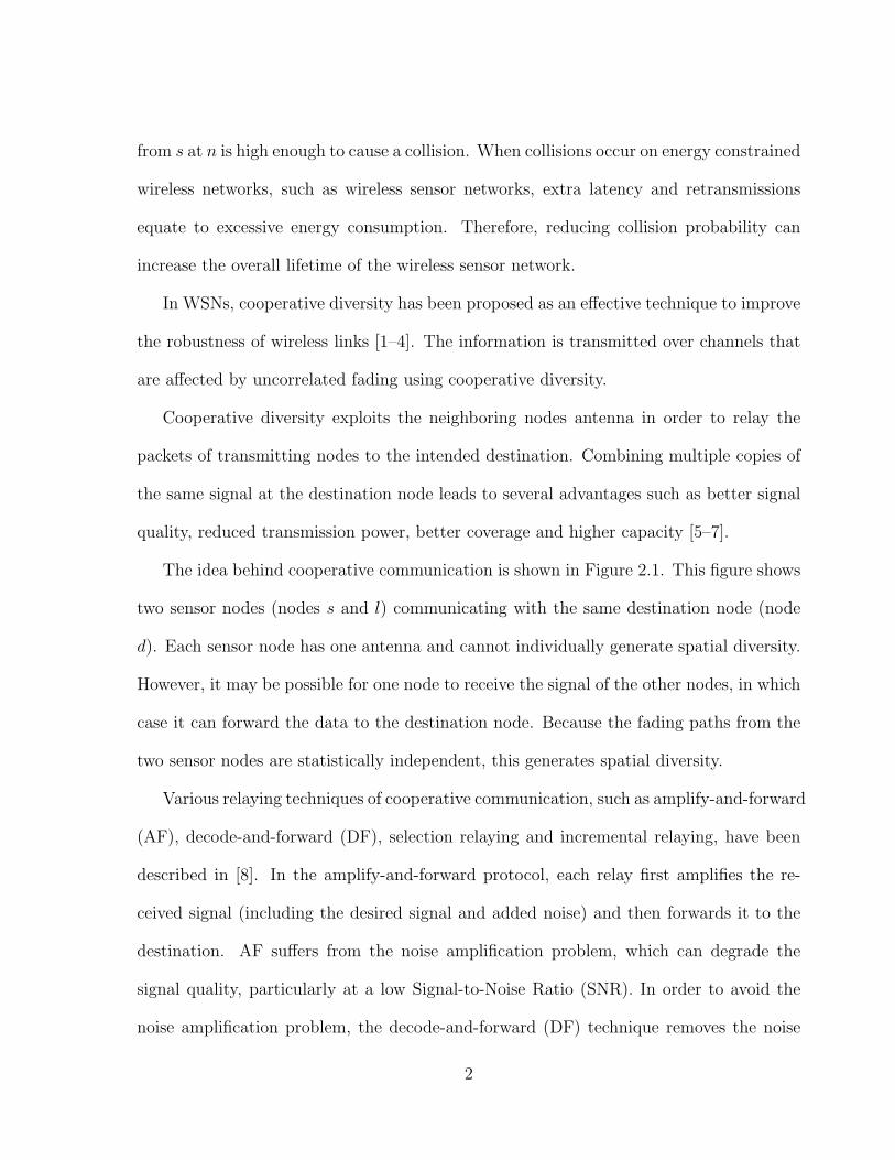
The idea behind cooperative communication is shown in Figure 2.1. This figure shows

two sensor nodes (nodes s and l) communicating with the same destination node (node

d). Each sensor node has one antenna and cannot individually generate spatial diversity.

However, it may be possible for one node to receive the signal of the other nodes, in which

case it can forward the data to the destination node. Because the fading paths from the

two sensor nodes are statistically independent, this generates spatial diversity.

Various relaying techniques of cooperative communication, such as amplify-and-forward

(AF), decode-and-forward (DF), selection relaying and incremental relaying, have been

described in [8]. In the amplify-and-forward protocol, each relay first amplifies the re-

ceived signal (including the desired signal and added noise) and then forwards it to the

destination. AF suffers from the noise amplification problem, which can degrade the

signal quality, particularly at a low Signal-to-Noise Ratio (SNR). In order to avoid the

noise amplification problem, the decode-and-forward (DF) technique removes the noise

2

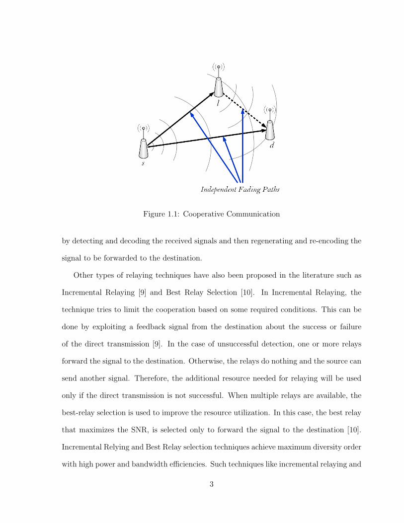
Figure 1.1: Cooperative Communication

by detecting and decoding the received signals and then regenerating and re-encoding the

signal to be forwarded to the destination.

Other types of relaying techniques have also been proposed in the literature such as

Incremental Relaying [9] and Best Relay Selection [10]. In Incremental Relaying, the

technique tries to limit the cooperation based on some required conditions. This can be

done by exploiting a feedback signal from the destination about the success or failure

of the direct transmission [9]. In the case of unsuccessful detection, one or more relays

forward the signal to the destination. Otherwise, the relays do nothing and the source can

send another signal. Therefore, the additional resource needed for relaying will be used

only if the direct transmission is not successful. When multiple relays are available, the

best-relay selection is used to improve the resource utilization. In this case, the best relay

that maximizes the SNR, is selected only to forward the signal to the destination [10].

Incremental Relying and Best Relay selection techniques achieve maximum diversity order

with high power and bandwidth efficiencies. Such techniques like incremental relaying and

3

best-relay selection can be used with AF, DF or any other relaying method.

In [1], cooperative diversity employs space-time coding, which is the 2 × 2 Alamouti

scheme, using cooperative relaying. This scheme is shown to improve link quality signifi-

cantly, and as a result, it reduces the packet dropping rate at the receiver and improves

the network throughput. In [2,3] a cooperative MAC protocol has been proposed to facil-

itate the use of cooperative diversity with adaptive relay selection in WSNs using signal

forwarding (by the relays) and Maximum Ratio Combining (MRC) at the destination.

As shown in both references, the proposed MAC protocol is able to improve the links

robustness, and therefore increases the throughput gain and reduces the packet dropping

rate significantly.

Routing algorithms which take into consideration the availability of cooperative trans-

mission at the physical layer are known in the literature as cooperative routing algorithms.

In other words, cooperative routing makes the use of cooperative diversity from the physi-

cal layer to benefit the network layer by improving the performance of routing. Therefore,

cooperative routing is a cross-layer design approach that combines the network layer and

the physical layer to transmit packets through cooperative links. This cross-layer de-

sign approach effectively enhances the performance of the routing protocols in wireless

networks.

In traditional multi-hop routing, messages are transmitted through multiple radio hops

and routing protocol is a concatenation of traditional hops. These traditional routing

protocols choose the best sequence of nodes between the source and the sink, and forward

each packet through that sequence using a single direct signal. In contrast, cooperative

routing takes the advantage of the broadcasting transmission to transmit the message

in each hop through relay nodes as well. Therefore, cooperative routing allows multiple

4

nodes along a path to coordinate together to transmit a message to the next hop as long

as the combined signal at the receiver node satisfies a given Signal-to-Noise Ratio (SNR)

threshold value. The receiver node in each hop selects the best of received signals (direct

or relayed), or combines them to produce a stronger signal.

For signal combining in cooperative routing, traditional diversity combining techniques

such as Maximum Ratio Combining (MRC), Equal Gain Combining (EGC), and Selection

Combining (SC) can be used by each receiver node along the path. Brennan described

the aforementioned techniques in [11]. In MRC, the received signals from all cooperators

are weighted and combined to maximize the instantaneous SNR. It is known that MRC is

optimal and maximizes the total SNR in noise-limited links with Gaussian noise. However,

the main drawback of the MRC technique is that it requires full knowledge of the channel

state information [8]. EGC is a simplified sub-optimal combining technique, where the

destination node combines the received copies of the signal by adding them coherently.

Therefore, the required channel information at the receiver node is reduced to the phase

information only. SC is even simpler and the combiner simply selects the signal with larger

SNR. Although, SC removes the overhead of estimating the channel state information, its

performance is ultimately degraded compared to MRC and EGC [8].

1.2 Research Motivation

As mentioned before, in addition to the energy constraint in wireless sensor networks,

another main fundamental limiting factor is the collision probability [12]. In some situ-

ations, for instance upon the detection of an event in wireless sensor networks, the data

exchange in certain areas spots may become intensified, resulting in a high packet collision

5

probability. A high packet collision rate causes a packet loss and leads to retransmission.

Retransmission increases the packet delay and energy consumption.

Packet collision in general wireless ad hoc network is usually addressed by the use

of Distributed Coordination Function (DCF). DCF provides a 4-way handshaking tech-

nique, known as Request-To-Send/Clear-To-Send (RTS/CTS) mechanism. RTS/CTS

mechanism is basically designed to reduce the number of collisions by reserving the chan-

nel around both the sender and the receiver to protect transmitted frame from corruption

caused by collision [13]. However, this method presents several problems when used in

wireless sensor networks. These problems include the following:

• the energy consumption related to a RTS/CTS packets exchange is significant,

• because data frames in wireless sensor networks are usually small and collision may

occur for RTS/CTS packets same as data frames, it does not make a significant

difference in collision probability if the technique is used or not,

• it may lower the network capacity due to the exposed node problem [14],

• it cannot be used for broadcasting frames.

Transmission collision in a wireless sensor network can be minimized by reducing the

collision probability. This can be achieved through the use of cooperative diversity tech-

niques. Cooperative diversity is beneficial for WSNs since the size and power constraints

restrict sensor nodes from possessing more than one antenna [15].

Although the merits of the cooperative communications in the physical layer have

been well-explored, the impact of the cooperative communications on the design of the

higher layers, such as routing protocols, has not yet been well-developed.

6

Routing is a key factor which plays an important role to the network performance, par-

ticularly in WSNs. Due to the restricted communication range and power budget, packet

forwarding in sensor networks is usually performed through multi-hop data transmission.

Therefore, routing in wireless sensor networks is crucial and challenging.

Routing protocols need to be redesigned for cooperative communication in wireless

networks because of three reasons. First, when cooperative communication is supported in

the physical layer, a link is no longer composed of one sender and one receiver. There may

be multiple nodes acting as the senders or as the receivers simultaneously. Therefore, the

definition of a traditional link which contains only two nodes (one sender and one receiver)

should be revised. With the revised link definition, routing, which is constructed based on

the concept of links, cannot remain unchanged. Second, cooperative diversity introduces

new aspects to the typical traffic load of the nodes in WSNs. A relay node in a cooperative

link not only receives traffic load from the transmitter node, but also forwards the traffic

load to the destination node. Third, with the introduction of cooperative communication,

the collision probability between multiple links is different. Therefore, a new routing

protocol should consider the differences in cooperative communication.

1.3 Thesis Contribution

This dissertation presents the following novel contributions to the optimal cooperative

route selection for minimizing the collision probability in WSNs.

We propose a novel and accurate mathematical model to analyse the per-node traffic

load in a cooperative link of WSNs.

7

We show the accuracy of the proposed per-node traffic load analytical model by

verifying the agreement between the analytical results and simulation.

We employ the proposed analytical model of per-node traffic load in cooperative

transmissions and we formally define and formulate the collision problem in WSNs.

We present a Mixed Integer Non-Linear Problem (MINLP) model for optimizing

the cooperative routing selection to minimize the collision problem subject to the

outage probability constraint.

We solve the optimization problem by enhancing the Branch and Bound (BnB)

algorithm and developing a BnB Space Reduction algorithm. The obtained solution

applies a joint optimization approach to power allocation, relay node assignment,

and path selection which are the main optimization issues in cooperative routing.

We also propose two near-optimal algorithms by decoupling the optimization vari-

able decisions from the other optimization parameters. In the first near optimal

cooperative routing, optimal power allocation and relay selection is decoupled from

the routing decision. In the second near optimal cooperative routing, optimal trans-

mission power is decoupled from the other optimization variables.

We illustrate that the MINLP solution serves as a benchmark for evaluating the

quality of the solutions obtained by any sub-optimal algorithm for this problem.

We evaluate the effect of each of the optimal routing parameters separately, by

developing addition routing algorithms, in which one optimization variable is used

while the other parameters are not employed.

8

We show that the proposed algorithms (optimal and near optimal) find good solu-

tions which help to reduce collision probability compared to the existing cooperative

routing algorithms.

1.4 Thesis Outline

In this section, we outline the organization of this thesis and give a brief overview of each

chapter.

In Chapter 2, we present a comprehensive survey of the existing cooperative routing

techniques, together with the highlights of the performance of each strategy. We also

provide a taxonomy of different cooperative routing protocols and outline the fundamen-

tal components and challenges associated with cooperative routing objectives. Moreover,

the design requirements of cooperative routing protocols are discussed to provide an in-

sight into the objectives of routing protocols. We compare existing cooperative routing

algorithms and lay the groundwork for further research.

Most of the proposed cooperative routing techniques are designed for single-flow net-

works and packet collision caused by multiple flows has not been taken into account. In

Chapter 3, packet collision probability is mathematically formulated and a sub-optimal

cooperative routing algorithm to minimize collision probability is proposed. In this chap-

ter, the problem is formulated assuming that the average per-node traffic load follows the

Poisson arrival process (this assumption is improved in Chapter 5, using the mathematical

analysis obtained in Chapter 4).

In Chapter 4, we present a new and detailed analytical model for calculating the per-

node traffic load in cooperative WSNs. Cooperative routing introduces a new aspect to the

9

typical per-node traffic load in multiple-flow networks. A relay node in a cooperative link

not only receives traffic load from the transmitter node, but also forwards the traffic load

to the destination node. To the best of our knowledge, there is no analytical model which

can accurately characterize the per-node traffic load in a cooperative wireless network.

Analysing the per-node traffic load in cooperative system helps to provide important

insights into designing efficient cooperative routing protocols.

The analytical model of the traffic load is employed in Chapters 5 and 6 to minimize

the collision probability using cooperative routing. We propose the Minimum Collision

Cooperative Routing (MCCR) algorithm by combining cooperative transmission, optimal

power allocation, and route selection in Chapter 5. The proposed algorithm in Chapter

5 is a sub-optimal routing due to the following reasons; (1) the optimal power allocation

technique is decoupled from the optimal route selection and (2) a suboptimal approach

is employed in the relay node selection and relay nodes are selected as the node closest

to the middle point of the transmitter and receiver nodes of each link.

In Chapter 6, we obtain the optimal solution by formulating the problem as a large-

scale Mixed Integer Non-Linear Programming problem. To solve the optimization prob-

lem, we also propose a solution based on the branch and bound algorithm augmented

with reducing the search space (branch and bound space reduced). To reduce the com-

putational complexity of the optimal solution, we propose a near-optimal cooperative

routing algorithm in Chapter 6. In the near-optimal algorithm, we solve the problem by

decoupling the optimal power allocation scheme from optimal route selection. Finally

in Chapter 7, we summarize the contributions presented in this dissertation and discuss

10

several potential extensions to our work.

REFERENCES

[1] L. Liu and H. Ge, “Space-time coding for wireless sensor networks with cooperative

routing diversity,” in Proc. Asilomar Conference on Signals, Systems and Computers,

vol. 1, Nov. 2004, pp. 1271–1275.

[2] M. Gokturk and O. Gurbuz, “Cooperative MAC protocol with distributed relay

actuation,” in Proc. IEEE Wireless Communications and Networking Conference

(WCNC’09), April 2009, pp. 1–6.

[3] ——, “Cooperation in wireless sensor networks: Design and performance analysis

of a MAC protocol,” in Proc. IEEE International Conference on Communications

(ICC ’08), June 2008, pp. 4284–4289.

[4] T. ElBatt, S. Krishnamurthy, D. Connors, and S. Dao, “Power management for

throughput enhancement in wireless ad-hoc networks,” in Proc. IEEE International

Conference on Communications (ICC ’00), June 2000, pp. 1506–1513.

[5] J. Laneman, D. Tse, and G. W. Wornell, “Cooperative diversity in wireless networks:

Efficient protocols and outage behavior,” IEEE Trans. Inf. Theory, vol. 50, no. 12,

pp. 3062–3080, Dec. 2004.

11

[6] T. Himsoon, W. Siriwongpairat, Z. Han, and K. J. R. Liu, “Lifetime maximization by

cooperative sensor and relay deployment in wireless sensor networks,” in Proc. IEEE

Wireless Communications and Networking Conference (WCNC’06), April 2006, pp.

439–444.

[7] A. Bletsas, A. Khisti, and M. Win, “Opportunistic cooperative diversity with feed-

back and cheap radios,” IEEE Trans. Wireless Commun., vol. 7, no. 5, pp. 1823–1827,

May 2008.

[8] M. H. Ahmed and S. S. Ikki, To Cooperate or not to Cooperate? That is the Question!

John Wiley and Sons, Ltd, 2011, pp. 21–33.



pp. 3062–3080, Dec. 2004.

[10] A. Bletsas, A. Khisti, D. Reed, and A. Lippman, “A simple cooperative diversity

method based on network path selection,” IEEE J. Sel. Areas Commun., vol. 24,

no. 3, pp. 659–672, March 2007.

[11] D. G. Brennan, “Linear diversity combining techniques,” Proc. IEEE, vol. 91, no. 2,

pp. 331–356, Feb. 2003.

[12] W. Ye and J. Heidemann, “Medium access control in wireless sensor networks,”

USC/Information Sciences Institute, Tech. Rep. ISI-TR-580, Oct. 2003.

[13] G. Bianchi, “Performance analysis of the ieee 802.11 distributed coordination func-

tion,” IEEE J. Sel. Areas Commun., vol. 18, no. 3, pp. 535–547, March 2000.

12

[14] A. Koubaa, R. Severino, M. Alves, and E. Tovar, “Improving quality-of-service in

wireless sensor networks by mitigating ”Hidden-Node Collisions”,” IEEE Trans. Ind.

Informat., vol. 5, no. 3, pp. 299–313, Aug. 2009.

[15] N. Shastry, J. Bhatia, and R. Adve, “Theoretical analysis of cooperative diversity

in wireless sensor networks,” in Proc. IEEE Global Telecommunications Conference,

(GLOBECOM ’05), vol. 6, Dec. 2005, pp. 3269–3273.

13

Chapter 2

Cooperative Routing in Wireless

Networks: A Comprehensive Survey

2.1 Abstract

Cooperative diversity has gained much interest due to its ability to mitigate multipath

fading without using multiple antennas. There has been considerable research on how

cooperative transmission can improve the performance of the physical layer. During the

past few years, the researchers have started to take into consideration cooperative trans-

mission in routing and there has been a growing interest in designing and evaluating

cooperative routing protocols. Routing algorithms that take into consideration the avail-

ability of cooperative transmission at the physical layer are known as cooperative routing

algorithms. This paper presents a comprehensive survey of the existing cooperative rout-

ing techniques, together with the highlights of the performance of each strategy. This

survey also provides a taxonomy of different cooperative routing protocols and outlines

14

the fundamental components and challenges associated with cooperative routing objec-

tives. Existing cooperative routing algorithms are compared to lay the groundwork for

further research.

2.2 Introduction

Cooperative communication has emerged as a promising approach for mitigating wire-

less channel fading and improving reliability of wireless networks by allowing nodes to

collaborate with each other. Nodes in cooperative communication help each other with

information transmission by exploiting the broadcasting nature of wireless communica-

tion [1–3]. In a cooperative transmission scheme, neighboring nodes are exploited as

relay nodes, in which they cooperate with the transmitter-receiver pair to deliver mul-

tiple copies of a packet to the receiver node through independent fading channels. The

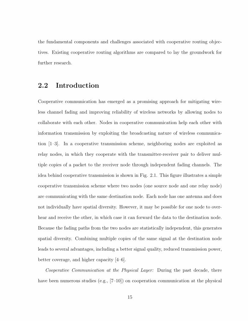
idea behind cooperative transmission is shown in Fig. 2.1. This figure illustrates a simple

cooperative transmission scheme where two nodes (one source node and one relay node)

are communicating with the same destination node. Each node has one antenna and does

not individually have spatial diversity. However, it may be possible for one node to over-

hear and receive the other, in which case it can forward the data to the destination node.

Because the fading paths from the two nodes are statistically independent, this generates

spatial diversity. Combining multiple copies of the same signal at the destination node

leads to several advantages, including a better signal quality, reduced transmission power,

better coverage, and higher capacity [4–6].

Cooperative Communication at the Physical Layer: During the past decade, there

have been numerous studies (e.g., [7–10]) on cooperation communication at the physical

15

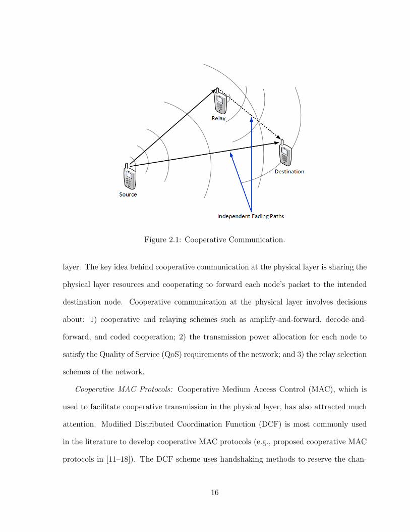
Figure 2.1: Cooperative Communication.

layer. The key idea behind cooperative communication at the physical layer is sharing the

physical layer resources and cooperating to forward each node’s packet to the intended

destination node. Cooperative communication at the physical layer involves decisions

about: 1) cooperative and relaying schemes such as amplify-and-forward, decode-and-

forward, and coded cooperation; 2) the transmission power allocation for each node to

satisfy the Quality of Service (QoS) requirements of the network; and 3) the relay selection

schemes of the network.

Cooperative MAC Protocols: Cooperative Medium Access Control (MAC), which is

used to facilitate cooperative transmission in the physical layer, has also attracted much

attention. Modified Distributed Coordination Function (DCF) is most commonly used

in the literature to develop cooperative MAC protocols (e.g., proposed cooperative MAC

protocols in [11–18]). The DCF scheme uses handshaking methods to reserve the chan-

16

nel and alleviate collision problems [19]. For the cooperative handshaking, additional

control signalling packets such as HTS (Helper ready To Send) in [11]; cRTS (coopera-

tive Request To Send) in [12]; RS (Relay-Start), RA (Relay-Acknowledgement), and RB

(Relay-Broadcasting) in [13] are introduced. The additional signalling packets are used

to select the relay nodes, indicate the presence of relay nodes and willingness for the

cooperative transmission, and demonstrate the availability of channel (i.e., check whether

the channel is not busy) for the relay nodes.

Cross-Layer Cooperative Communication: With better understanding of the cooper-

ative communication in the physical layer and the cooperative MAC protocols, it has

become critically important to study how the performance gain of cooperative communi-

cation in the physical and MAC layers can be reflected to upper layers (such as the network

layer), ultimately improving the performance using cooperative routing and cross-layer

cooperative protocols [20–22]. A routing algorithm that takes the advantages of coop-

erative transmission in the physical layer is known as cooperative routing. Cooperative

routing is a cross-layer design approach that combines the network layer and the physical

layer to transmit packets through cooperative links. This cross-layer design approach

effectively enhances the performance of the routing protocols in wireless networks.

In the past few years, significant progress has been made on the design and devel-

opment of cooperative routing protocols. These cross-layer routing protocols optimize

various aspects of cooperative communication. Cooperative routing is a promising ap-

proach to improving energy efficiency (or saving power) and QoS; it saves energy by

reducing path loss and combining multiple copies of the same packet at the receiver node.

Path loss is reduced by shortening the link length, which generates less interference due

to the lower transmission power. Moreover, optimal power allocation at the transmitter

17

and relay nodes (using power allocation techniques) can further reduce the energy (or

power) consumption.

In traditional multi-hop routing, messages are transmitted through multiple radio hops

and the routing protocol is a concatenation of traditional hops. These traditional routing

protocols choose the best sequence of nodes between the source and the sink, and forward

each packet through that sequence using a single direct signal. In contrast, cooperative

routing takes the advantage of the broadcasting transmission to transmit the message

in each hop through relay nodes as well. Therefore, cooperative routing allows multiple

nodes along a path to coordinate together to transmit a message to the next hop as long

as the combined signal at the receiver node satisfies a given Signal-to-Noise Ratio (SNR)

threshold value. The receiver node in each hop selects the best of received signals (direct

or relayed), or combines them to produce a stronger signal.

In this chapter, a comprehensive survey of the existing cooperative routing algorithms

is presented and the important aspects, requirements, challenges, and aims to design

cooperative routing algorithms are discussed. In this paper, we provide a taxonomy

of different cooperative routing protocols and we analyze various algorithms within the

groups with common characteristics. We also briefly discuss the most significant and well-

cited cooperative routing algorithms and compare the performance of the algorithms.

The remaining part of this chapter is organized as follows: In Section 2.3, a background

of cooperative routing is given. Section 2.4 provides a taxonomy of state-of-the-art co-

operative routing schemes and classifies the existing cooperative routing algorithms in

terms of 1) optimality, 2) objective function, and 3) centralization. Section 2.5 discusses

the optimality of cooperative routing algorithm. Section 2.6 explains the cooperative

routing objectives and aims. The objectives include energy-efficiency, QoS parameters,

18

and collision minimization. Section 2.7 presents a review on centralized and distributed

cooperative routing algorithms. Section 2.8 provides a brief overview of some existing

cooperative routing algorithms. The performance evaluation and comparison of the pro-

posed cooperative routing algorithms and challenges are presented in Section 2.9, and

finally, Section 2.10 concludes the chapter and presents some future research directions.

2.3 Background of Cooperative Routing

In general, a cooperative route is a concatenation of cooperative-transmission and direct-

transmission links. Fig. 2.2 shows an example of cooperative routing. The direct-

transmission (DT ) block is represented by the link (a, b), where node a is the transmitter

node and node b is the receiver node. The cooperative-transmission (CT ) block is rep-

resented by the links (i, j), (i, k), and (k, j), where i is the transmitter node, k is a relay

node, and j is the receiver node. In cooperative transmission, in addition to the direct

link from the transmitter node to the receiver node, one or more relay nodes can be

used to relay the signal to the receiver node. Therefore, the definition of the traditional

link, which includes only two nodes, should be revised. In order to facilitate cooperative

communication, researchers need to address the requirements for designing cooperative

systems. These requirements include making decisions about the cooperative transmis-

sion scheme, relay node selection, resource allocation, channel state information, and the

cooperative routing metrics. In the entire chapter, we define the source node as the initial

transmitter node and the destination node as the final receiver node.

19

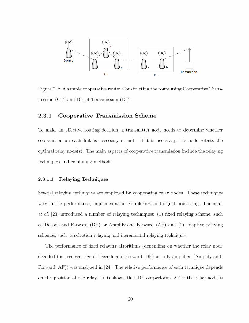
Figure 2.2: A sample cooperative route: Constructing the route using Cooperative Trans-

mission (CT) and Direct Transmission (DT).

2.3.1 Cooperative Transmission Scheme

To make an effective routing decision, a transmitter node needs to determine whether

cooperation on each link is necessary or not. If it is necessary, the node selects the

optimal relay node(s). The main aspects of cooperative transmission include the relaying

techniques and combining methods.

2.3.1.1 Relaying Techniques

Several relaying techniques are employed by cooperating relay nodes. These techniques

vary in the performance, implementation complexity, and signal processing. Laneman

et al. [23] introduced a number of relaying techniques: (1) fixed relaying scheme, such

as Decode-and-Forward (DF) or Amplify-and-Forward (AF) and (2) adaptive relaying

schemes, such as selection relaying and incremental relaying techniques.

The performance of fixed relaying algorithms (depending on whether the relay node

decoded the received signal (Decode-and-Forward, DF) or only amplified (Amplify-and-

Forward, AF)) was analyzed in [24]. The relative performance of each technique depends

on the position of the relay. It is shown that DF outperforms AF if the relay node is

20

closer to the transmitter node, and AF outperforms DF if the relay node is closer to the

receiver node [24]. From a practical point of view, it is still debatable which scheme is

easier to implement. DF may offer higher complexity because of the decoding requirement

at the relay node. On the other hand, AF may be problematic in terms of data storage

in analogue format [25].

Fixed relaying techniques need twice the time to transmit a data packet from the

source to the destination node compared to the direct transmission technique. As a

result, the throughput of the fixed relaying schemes can be degraded compared to that

of the direct transmission. In addition, when the destination node can correctly decode

the data packets transmitted from the source in the first time slot, the channel resource

of the second time slot exploited by the relay node is wasted. To combat these problems,

adaptive relaying methods that effectively use the channel resources are proposed in [1].

The authors described two adaptive relaying protocols: selection relaying and incremental

relaying. Selection relaying allows transmitter nodes to select a suitable relay node based

on the measured SNR. With the incremental relaying technique, the source node sends

its signal to the destination node, using a direct link. If the destination node is unable to

detect the signal using the direct link, the relay node forwards the signal to the destination

node (provided that the relay node was able to detect the signal). If the relay node is

unable to detect the signal, it will remain silent. Selection relaying and incremental

relaying can be used with either AF or DF.

2.3.1.2 Combining Techniques

For signal combining in cooperative routing, traditional diversity combining techniques

such as Maximum Ratio Combining (MRC), Equal Gain Combining (EGC), and Selection

21

Combining (SC) can be used by each receiver node along the path. Brennan described

the aforementioned techniques in [26]. In MRC, the received signals from all coopera-

tors are weighted and combined to maximize the instantaneous SNR. It is known that

MRC is optimal and maximizes the total SNR in noise-limited links with Gaussian noise.

However, the main drawback of the MRC technique is that it requires full knowledge of

the channel state information [27]. EGC is a simplified sub-optimal combining technique,

where the destination node combines the received copies of the signal by adding them

coherently. Therefore, the required channel information at the receiver node is reduced

to the phase information only. SC is even simpler and the combiner simply selects the

signal with larger SNR. Although, SC removes the overhead of estimating the channel

state information, its performance is ultimately degraded compared to the MRC and

EGC [27]. In addition to the aforementioned combining techniques, Optimal Combining

(OC) is proposed for the interference-limited links in the literature [28, 29]. With Op-

timal Combining, signals received from the transmitter and relay nodes are weighted to

maximize the Signal Interference Ratio (SIR) at the receiver node. However, OC requires

the instantaneous Channel State Information (CSI) of all interferers to be known at the

receiver, and hence, demands significant system complexity [30].

2.3.2 Relay Node Selection

Relay node selection is crucial for the performance of cooperative routing because a good

quality relay node yields a higher diversity gain. Therefore, optimal relay node selection

potentially enhances the system performance and achieves the cooperative routing ob-

jectives such as energy efficiency, throughput, and packet delivery ratio. The relay node

22

selection strategies in terms of the optimal number of relay nodes and optimal relay node

location are briefly described below.

2.3.2.1 Optimal number of relay nodes

Intuitively, exploiting more relay nodes will lead to a higher diversity gain and better

performance. However, more relay nodes need more resources (such as more time slots)

and cause a larger interference area (containing the set of nodes that would cause inter-

ference at the receiver, if they also transmitted [31]), which may reduce the cooperation

gain. Without a central controller, more coordination overhead is involved in selecting

more relay nodes. Due to the protocol overhead, the energy efficiency of cooperative

transmission degrades with the increase of the number of relay nodes. The authors in [14]

demonstrated that there is a direct relationship between the interference area and the

number of relay nodes; the interference area affected by cooperation is enlarged propor-

tionally to the number of relay nodes. Therefore, the overall throughput performance may

degrade. It is proved in [32,33] that selecting only the single best relay node accomplishes

the same diversity gain as that of multi-relay cooperation.

2.3.2.2 Optimal relay node placement

In addition to the number of relay nodes, the potential gain of a cooperative route depends

on the location of the relay nodes. The best relay node is the one that can enhance the

objective performance to the maximum extent. The definition of the best relay node

depends on the application scenario. For instance, in [34], in which the routing objective

is the energy efficiency, if the minimum energy consumption of a cooperative-transmission

link corresponds to a certain relay node, that specific node is selected as the best relay

23

node for the transmitter node. For links with a single relay node, Wang et al. [35] showed

how game theory [36] can be used to select the best cooperative relay node. For links with

multiple relay nodes (i.e., multi-relay based cooperative links), the authors in [37] proved

that the optimal performance is achieved when all the cooperative nodes appear to be

at the same distance from the destination node. In addition, Astaneh and Gazor in [38]

demonstrated that, for the DF relaying scheme, the best location for the relay node is in

the vicinity of the midpoint between the transmitter-receiver pair in each link.

2.3.3 Resource Allocation in Cooperative Communication

When a feedback channel in cooperative links is available, adaptive resource allocation

can make significant performance enhancement by adapting transmission parameters to

the channel characteristics. The existing resource allocation strategies of cooperative

links can be divided into two categories: optimal resource allocation and equal resource

allocation.

Optimal resource allocation has been addressed in many studies, such as [39–42], and

the authors have dealt with various aspects of resource allocation, in terms of power

[42], bandwidth [40], and time [41]. The optimization techniques and heuristic decision

making algorithms are employed to allocate optimal resources to the transmitter and relay

nodes. For instance, the Lagrangian method is used in [21, 37, 42–44] to allocate optimal

transmission power of transmitter and relay nodes. Moreover, authors in [40] employed

Stackelberg differential game models (described in [36]) as the heuristic decision making

algorithms to allocate joint bandwidth and the power of the transmitter and relay nodes

in the cooperative-transmission links.

24

Although equal resource allocation strategies are not optimal, the simplicity of the

equal resource allocation algorithms make them more suitable for implementation [45,46].

2.3.4 Channel State Information (CSI)

In order to adapt to the channel statistics, most of the existing cooperative schemes take

the availability of CSI at transmitter nodes into consideration to evaluate the effectiveness

of cooperation and to coordinate the relay node selection. In a cooperative link, the

receiver nodes utilize the available CSI for coherent reception, and the transmitter nodes

can utilize the available CSI for power control, signal combining, and relay selection.

To estimate a channel coefficient, a pilot message is usually sent out by the transmitter

nodes, and then the receiver nodes exploit the known pilot message to estimate the channel

coefficient.

The majority of the work on cooperative communication has focused on the scenarios

in which the CSI is available at the transmitter and receiver nodes in the form of accurate

estimates for the fading coefficients. However, because of the errors that can occur in the

channel estimation, a perfect CSI is hard to obtain practically. A central unit can be used

to collect the accurate CSI of all links, to schedule the transmission, and to coordinate

the cooperative behaviours (e.g., [42, 43, 47]). However, the centralized policies are not

efficient in large networks or in networks where the traffic is relatively low. Therefore, the

authors in [48–50] developed distributed algorithms that require far less CSI and yield a

performance nearly as good as the centralized cooperative transmission with CSI, while

outperforming the direct transmission.

The performance of cooperative communication in the presence of imperfect CSI is

25

investigated in the literature, such as [51–53]. The relay selection and power allocation in

the consideration of CSI imperfection are performed in [51] by means of the correlation

coefficient of the estimated channel gain and its actual values. It is shown in [53] even

though the transmitter nodes have imperfect CSI, cooperative transmission can signifi-

cantly improve the overall system performance compared to the direct transmission.

2.3.5 Network Coding in Cooperative Diversity

Network coding is an efficient technique that allows intermediate nodes to encode and

combine incoming packets instead of only copying and forwarding them. Network coding

has been recognized as a promising technique to increase system throughput, and also

is the basis for many bandwidth and energy-efficient transmission schemes in wireless

networks [54–56]. While there are many papers, such as [57], addressing network coding

in cooperative diversity, there are only a few papers discussing the network coding in

cooperative routing (e.g. [7]). In [7], the cooperative Physical Layer Network Coding

(CPLNC) scheme (physical layer network coding is discussed in [58]) is applied to an

optimal non-cooperative shortest path route. After choosing the shortest path route,

the first symbol is transmitted non-cooperatively between the source and the destination

node. If CPLNC consumes less power than non-cooperative transmission for the given

hop, from the second symbol onwards, for each group of three consecutive nodes along

the route, the first two nodes transmit cooperatively to the third node. Simulation results

in [7] proved that the network coding in cooperative routing outperforms the conventional

network coding in terms of energy saving gains.

26

2.3.6 Cooperative Routing Metrics

A routing metric is a function of the routing objective(s) and demonstrates the cost

values used by routing protocols to determine whether one particular route should be

chosen over another. Therefore, the routing cost metric, which affects the path selection

and resource consumption, is a crucial element of the routing protocol design. To perform

cooperative routing, a metric calculation is performed for each cooperative link, including

the potential relay node in an available cooperative transmission scheme. According to

the various applications of the cooperative networks, the routing metrics include energy

consumption (e.g., [42]), throughput (e.g., [59]), packet delivery ratio (e.g., [60]), and

collision probability (e.g., [61]).

Most of the proposed cooperative routing algorithms, such as [42, 59], rely on the

use of only a single cost metric. However, the single-metric approach is not adequate

for future wireless networks for the following reasons: firstly, some applications might

have multiple performance requirements that should be met simultaneously during the

route discovery; secondly, developing new wireless communication technologies produces

a wide range of wireless devices with different levels of constrained resources. Therefore,

multi-metric cooperative routing algorithms are developed in the literature. For instance,

in [60], cooperative routing metrics include throughput, packet delivery ratio, and energy

efficiency. In other words, the algorithm in [60] decides what route is preferred based on

the achievable throughput, packet delivery ratio, and energy efficiency. This is achieved

by combining all these routing metrics in the routing cost function.

27

2.3.7 Cooperative Routing Applications

Each cooperative routing algorithm has a specific application in a given scenario and can

be designed to allow the network to cope with the demands of a particular application.

Thus, the performance of a cooperative routing protocol may vary dramatically with

different network applications. It is very difficult to make a comprehensive cooperative

routing suitable for all applications. Thus, cooperative routing is formulated according to

the network application. For instance, in [43], cooperative routing is applied in a sensor

network and problem formulation corresponds to the total remaining energy, which is

the most important performance measure in WSNs due to the limited power supply.

Therefore, the objective function is the remaining energy. WSNs play an important role

in vast applications, such as environmental monitoring and target detection. In [62], the

cooperative routing is formulated for rate maximization in a cellular network and each

mobile station has the option of routing a tone signal in a cell through the other mobile

stations in the cell.

2.4 Taxonomy of Cooperative Routing Protocols

In order to evaluate the state-of-the-art cooperative routing algorithms, first a taxonomy

should be defined and various algorithms should be compared and analysed within the

groups with common characteristics. Cooperative routing algorithms are classified based

on three main characteristics: 1) optimality, 2) objective, and 3) centralization. The

taxonomy of cooperative routing protocols is illustrated in Fig. 2.3.

28

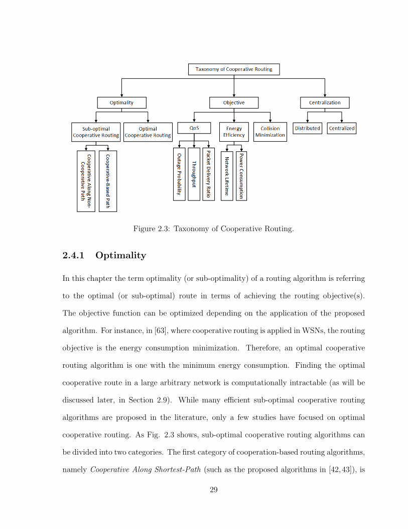
Figure 2.3: Taxonomy of Cooperative Routing.

2.4.1 Optimality

In this chapter the term optimality (or sub-optimality) of a routing algorithm is referring

to the optimal (or sub-optimal) route in terms of achieving the routing objective(s).

The objective function can be optimized depending on the application of the proposed

algorithm. For instance, in [63], where cooperative routing is applied in WSNs, the routing

objective is the energy consumption minimization. Therefore, an optimal cooperative

routing algorithm is one with the minimum energy consumption. Finding the optimal

cooperative route in a large arbitrary network is computationally intractable (as will be

discussed later, in Section 2.9). While many efficient sub-optimal cooperative routing

algorithms are proposed in the literature, only a few studies have focused on optimal

cooperative routing. As Fig. 2.3 shows, sub-optimal cooperative routing algorithms can

be divided into two categories. The first category of cooperation-based routing algorithms,

namely Cooperative Along Shortest-Path (such as the proposed algorithms in [42, 43]), is

29

implemented by finding the shortest-path route first, and then building the cooperative

route based on the shortest path. The main idea of algorithms in this category is to

use cooperative transmission to improve performance along the selected non-cooperative

links. However, the optimal cooperative route might be completely different from the

non-cooperative shortest path. Therefore, the merits of cooperative routing are not fully

exploited if cooperation is not taken into account while selecting the route. The algorithms

in the second category, Cooperative-Based Path (e.g., the proposed algorithms in [34, 45,

64, 65]), address the above problem by exploiting cooperative communication during the

route selection process. However, the algorithms in this category are not optimal due

to the following reasons: (1) they employ the sub-optimal approaches in the relay node

selection [45], power allocation [34], or route selection [64] and (2) they utilize optimal

relay node selection, resource allocation, and route selection but not jointly (as will be

discussed in detail in Section 2.5), such as algorithm in [65].

2.4.2 Objective

The objective of cooperative routing is defined as the target of the cooperative routing

algorithm. As Fig. 2.3 illustrates, the targets of cooperative routing algorithms in the

literature can be classified into three categories: (1) energy-efficiency (e.g., [34]), (2) QoS

parameters including throughput (e.g., [59]), packet Delivery Ratio (PDR) (e.g., [60]),

and outage probability (e.g., [66]), and (3) collision minimization (e.g., [61]). Overall,

energy efficiency is the most common objective of cooperative routing algorithms because

cooperative communication is a promising approach for energy saving.

30

2.4.3 Centralization

Cooperative routing decisions are made based on the information of the network. The

information of the network can be obtained by either: (1) using a centralized controller

in a centralized mode, or (2) having each node be responsible for obtaining network infor-

mation by itself and making a routing decision in a distributed mode, Fig. 2.3 illustrates

these two categories. Therefore, the main difference between the centralized and dis-

tributed cooperative routing algorithms is the place where the information is obtained

and route decision is made. Having a centralized controller may not be possible in some

wireless networks, such as ad hoc networks [67]. Moreover, the centralized routing algo-

rithms are not scalable, particularly in cooperative routing where a complete view of the

network including all cooperative links and relay nodes is needed.

In the following three sections, we elaborate on cooperative routing algorithms in the

three taxonomic groups, optimality, objective, and centralization, and we discuss the key

ideas of cooperative routing algorithms in each group.

2.5 Cooperative Routing Optimality

2.5.1 Optimal Cooperative Routing Schemes

Only algorithms proposed in [63, 68] have focused on optimal cooperative routing. The

algorithms in these two papers present frameworks to demonstrate the exact formulation

for the optimal relay node and optimal power allocation set, and jointly use of optimal

power, relay node allocation, and path selection. The frameworks lead to a Mixed-Integer

Linear Programming problem (MILP). In [68], the branch and bound cutting plane al-

31

gorithm is utilized to solve the MILP problem and obtain the optimal cooperative route.

In [63], the MILP problem contains n + 2 real decision variables (nr) and n + 2 binary

decision variables (nb), as well as 4n+ 9 inequalities, where n is the maximum number of

neighboring relay nodes. The author proved that obtaining the solution, in the worst-case

scenario, requires complexity of O(2nb). Therefore, the complexity of the computations

required to solve these problems grows exponentially with the number of binary deci-

sion variables. Given these points, the initial price for achieving optimal performance

is a more complex optimization framework. To ease the implementation of these ap-

proaches, powerful techniques, such as multi-parametric programming, are carried out

off-line. Multi-programming techniques are utilized to find an explicit solution to the op-

timization problem. Hence, the major parts of the computation can be performed before

the system starts its operation.

2.5.2 Sub-Optimal Cooperative Routing

As mentioned before, due to the required computational complexity of finding optimal

cooperative routing, heuristic sub-optimal cooperative routing algorithms are proposed

in the literature.

2.5.2.1 Cooperative Along Non-cooperative Path

The key idea in this category is applying cooperative communication techniques to im-

prove performance along the selected non-cooperative path. In other words, the coopera-

tive communication is implemented after non-cooperative path selection. Non-cooperative

path, which is an underlying path, is decided based on the traditional single link routing

algorithms. Normally, the underlying non-cooperative paths attempt shortest-path meth-

32

ods to achieve the cooperative routing objective(s). After establishing the non-cooperative

path, relay node selection is performed using one of the following sub-optimal methods:

employing the last few nodes along the selected non-cooperative path as the relay

nodes, as it is implemented in [42,43];

using contention among nodes (i.e., nodes are involved in the competition) to find

the relay node that has the best performance (such as longer connection time in [67])

among the neighboring nodes, as it is used in [67,69];

utilizing the nodes’ location information firstly to find the potential relay set (e.g.,

nodes located in the coverage intersection area of transmitter and receiver nodes,

i.e., node is covered by both transmitter and receiver nodes [59] as shown in Fig.

2.4) or nodes closest to the destination node in [70]), and then assigning a weight

to the potential relay nodes. The weight of each node represents the achievable

performance when that particular node acts as the relay node. Finally, the nodes

which lead to the best performance are selected.

The computational complexity of the sub-optimal cooperative routing algorithms in

this category mainly depends on the complexity of the underlying non-cooperative path.

For instance, in [42], the complexity of the proposed algorithm is the same as finding the

non-cooperative shortest path in the network (O (N2), where N is the total number of

nodes in the network).

2.5.2.2 Cooperative-Based Path

The optimal cooperative route might be completely different from the underlying non-

cooperative shortest path selected without taking cooperative links into consideration.

33

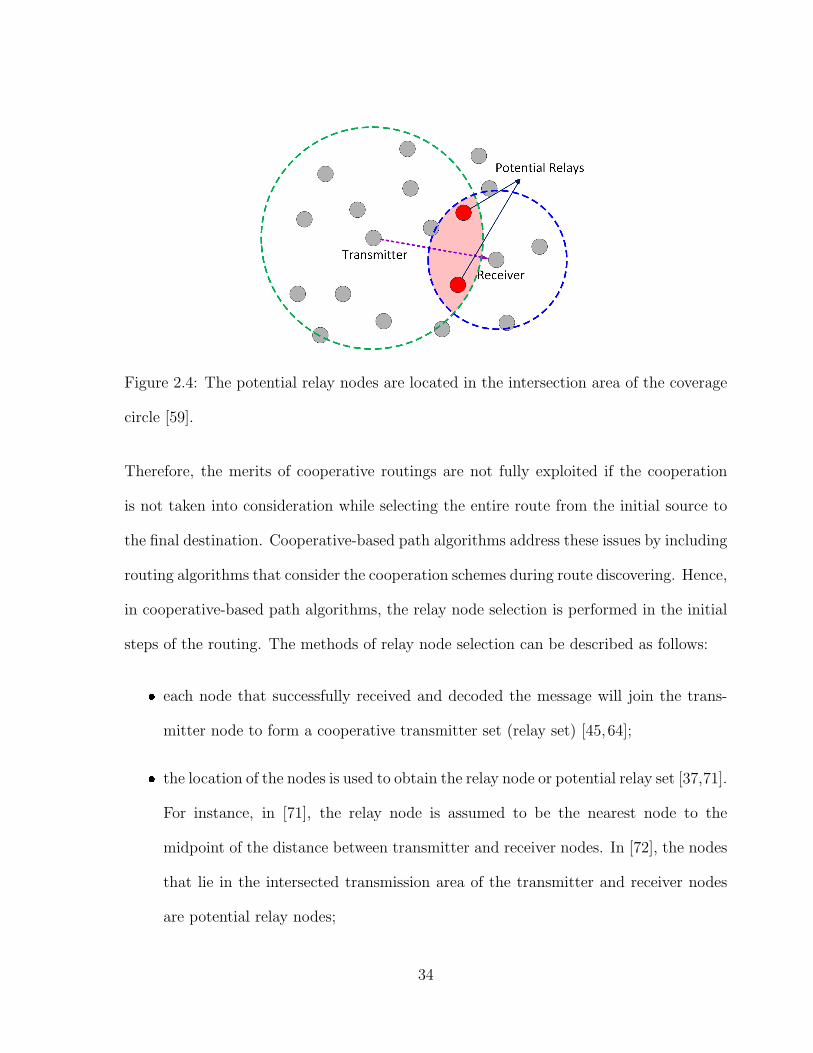
Figure 2.4: The potential relay nodes are located in the intersection area of the coverage

circle [59].

Therefore, the merits of cooperative routings are not fully exploited if the cooperation

is not taken into consideration while selecting the entire route from the initial source to

the final destination. Cooperative-based path algorithms address these issues by including

routing algorithms that consider the cooperation schemes during route discovering. Hence,

in cooperative-based path algorithms, the relay node selection is performed in the initial

steps of the routing. The methods of relay node selection can be described as follows:

each node that successfully received and decoded the message will join the trans-

mitter node to form a cooperative transmitter set (relay set) [45,64];

the location of the nodes is used to obtain the relay node or potential relay set [37,71].

For instance, in [71], the relay node is assumed to be the nearest node to the

midpoint of the distance between transmitter and receiver nodes. In [72], the nodes

that lie in the intersected transmission area of the transmitter and receiver nodes

are potential relay nodes;

34

all neighboring nodes are investigated and the node corresponding to the minimum

cost function is selected [34];

the potential relay set or the relay node candidates compete to determine the short-

est back-off time (usually, back-off time is inversely proportional to the routing

objective; for instance, node that lead to the highest throughput should have short-

est back-off time) and when the first back-off time expires, the corresponding relay

node is selected [66].

After selecting the relay nodes and potential cooperative links, route selection is per-

formed by applying shortest-path algorithms or dynamic routing protocols [73]. For in-

stance, the Bellman-Ford algorithm is employed in cooperative links in [34], while Dijk-

stra’s algorithm is used in [64].

However, the algorithms in this category are still sub-optimal because of the following

reasons: assumptions, such as assigning M levels for the transmission power in [71];

approximations, such as approximating of the exponential function using the first term

of the Taylor series to simplify the analytical expressions in [34]; sub-optimal relay node

selection, such as assigning the nearest node to the midpoint of the distance between

transmitter and receiver nodes in [71] or selecting any nodes that successfully received

and decoded the message as the relay node [45]; non-optimal power allocation methods,

such as equal power allocation to the transmitter and relay nodes in [37, 73]; not jointly

implementing the optimal relay selection, resource allocation, and route selection [65].

The computational complexity of cooperative-based routing algorithms depends both

on constructing the cooperative links and selecting cooperative routes. For instance, in

[34] with N nodes in the network, the worst case computational complexity of calculating

35

the possible relay node at each transmitter node is N , and the complexity of calculating

the cooperation cost at each node is O (N2); therefore, the complexity of the algorithm is

O (N3).

2.6 Cooperative Routing Objectives

2.6.1 Energy-Efficient Cooperative Routing

Saving energy (or power) is one of the main objectives of routing algorithms in the deploy-

ment of various wireless networks, including ad-hoc networks [74,75], sensor networks [76],

personal area networks [77], and other wireless networks. Energy efficient cooperative

routing algorithms can be classified into two categories. In the first category, the target

is to minimize the total energy consumption for the end-to-end transmission. The co-

operative routing algorithms presented in [34, 42, 45, 60, 66, 69] are good examples of this

category. In most cooperative routing algorithms in this category, such as [34,42], energy

saving is achieved by minimizing the total transmission power of transmitter and relay

nodes. Therefore, the problem is formulated as the transmission power minimization.

For a given source-destination pair, Ω denotes all possible routes from the source node to

the destination node, where each route is defined as a set of hops or intermediate nodes

between the source and destination. For a route ω ∈ Ω, ωi denotes the i-th hop of this

route. Thus, the problem can be formulated as

Minω∈Ω

∑ωi∈ω

Pωi (2.1)

where Pωi denotes the transmission power over the i-th hop.

36

In the second category, the goal of the algorithms is to prolong the network lifetime,

such as algorithms in [43,70,72,78–80]. One definition of the network lifetime is the time

until the first node dies; this definition is widely used in the literature [43,72,79].

The algorithms in the first category focus only on minimizing the total energy con-

sumption from the source node to the destination node; however, consistently using the

minimum cost path for routing may lead to an unbalanced energy distribution among

nodes. This problem is addressed in the algorithms proposed in the second category. The

authors in [43, 70, 72, 78] employ the cooperative routing scheme to balance the energy

distribution among nodes in the network, which prolongs the network lifetime. This is

achieved by taking into account the residual energy of nodes when selecting nodes for the

route (either as the next hop or the relay node). However, implementing the balanced

data routing algorithm may be challenging because of heterogeneity among nodes, which

is inherited from the physical world as a result of different amounts of nodal traffic, data

transmission rates, and bandwidth ranges [81].

All energy-saving algorithms proposed either in the first category or in the second

category show high energy saving gains under different network conditions and constraints.

However, the power consumption of active radio electronics is not taken into account,

except in [37]. This study takes into consideration the radio electronics consumed power

that can increase significantly as a result of cooperative transmission by multiple nodes

(transmitter and relay nodes) to the next hop receiver node along the cooperative path.

In general, energy saving in cooperative routing algorithms is obtained by employ-

ing three mechanisms, namely Energy-Efficient Cooperative Link, Energy-Efficient Relay

Node Assignment, and Energy-Efficient Path Selection, or any combination of these tech-

niques.

37

2.6.1.1 Energy-Efficient Cooperative Link

In this strategy, the algorithms first calculate a cost function for each cooperative link

based on the minimum transmission power and then energy-saving links are employed to

find the minimum energy routing scheme. The link’s cost calculation is performed using

various approaches, such as allocating minimum transmission power under certain network

constraints (e.g., outage probability constraint). Energy efficient cooperative link selection

strategy is used in [34, 42, 43, 45, 47, 66, 69]. Algorithms proposed in [42, 43, 69] are in

the Cooperation Along Non-cooperative Path category; therefore, minimum transmission

power is employed for non-cooperative links. Algorithms proposed in [34,45,47,66] are in

the Cooperative-Based Path category; therefore, minimum transmission power is employed

for either cooperative or non-cooperative links, which leads to less energy consumption.

2.6.1.2 Energy-Efficient Relay Node Assignment

In addition to the energy-efficient cooperative link selection methods, energy-efficient relay

node selection is an effective approach to save energy in cooperative routing algorithms.

In most of the energy-efficient relay node assignment approaches, a weight is assigned to

each relay node candidate. In algorithms presented in [34, 69], the weight represents the

amount of power consumption that can be saved if a particular node acts as a cooperative

relay node for the specific link. The link checks the weight of all possible relay nodes, and

the relay node with the minimum cost function is selected for the corresponding link. In

cooperative routing algorithms presented in [70, 72], the rely node candidates are sorted

in a descending order based on their remaining lifetime and the algorithm greedily picks

the nodes with the longer remaining lifetime and uses them as the relay nodes. Some

38

algorithms, such as those in [42,47], select the last few nodes in the minimum energy non-

cooperative path as the relay nodes. Finally, the algorithm in [37] determines the relay

node’s location that minimizes the transmission power and a super-node is considered as

if it is placed at this optimal location virtually. Each of the transmitting nodes adjusts

its phase with respect to the super-node, such that all the nodes appear to be at the same

distance from the destination.

2.6.1.3 Energy Efficient Path Selection

In addition to the strategies mentioned above, the minimum energy non-cooperative path

(as the underlying path in Cooperation Along Non-cooperative Path category) or minimum

energy cooperative path (among the cooperative weighted links in Cooperative-Based Path

category) can be obtained by employing the shortest-path algorithms, such as Dijkstra’s

algorithm [42,47], Bellman-Ford algorithm [34,72], and Suurballe’s algorithm [69].

2.6.1.4 Combination of The Aforementioned Techniques

Any combination of the energy-efficient strategies mentioned above leads to saving energy

in cooperative routing. In [34], Energy Efficient Relay Assignment and Energy-Efficient

Cooperative Link are combined to save energy utilizing cooperative routing.

2.6.2 QoS-Aware Cooperative Routing

The QoS in proposed cooperative routing algorithms is characterized by the following

parameters in the network: (1) throughput (as in [59, 64, 67, 68, 73]), (2) packet delivery

ratio (as in [60,80]), and (3) outage probability (as in [34,43,63,65,66,69,82]). In addition

to energy efficiency, QoS is also an important criterion to measure the performance of the

39

network. In critical applications, such as security, fire detection, and health monitoring,

QoS is a major concern [83, 84]. The goal of QoS in cooperative routing is to find a net-

work path that satisfies given constraints and simultaneously optimizes the utilization of

resources. QoS-Aware Cooperative Routing algorithms are classified into three categories

as follows.

1) Throughput-Aware Cooperative Routing Algorithms maximize the network through-

put. The network throughput can be defined as the number of successfully delivered

packets at the destination node in time unit [85]. The throughput in a wireless system

is limited by a number of factors, such as wireless channel characteristics (e.g., SNR and

bandwidth), end-to-end delay, network congestion, and collisions. Throughput optimiza-

tion cooperative routing algorithms are presented in [59,60,64,67,68,73].

In [59], each node across the selected non-cooperative path calculates the throughput

gain obtained by each potential relay node. The throughput of each cooperative link is

formulated by the channel capacity of the link and Shannon’s Theorem [86] is employed

to obtain the maximum capacity (i.e., throughput) of the cooperative link. By comparing

the throughput gains when different nodes are selected for a cooperative link, the node

that leads to the maximum throughput gain is selected as the relay node. This method is

employed in [60], where the throughput of cooperative links are compared and the coop-

erative link which leads to the maximum throughput is selected. Moreover, cooperative

routing algorithms presented in [64, 67, 73] increase the throughput in wireless networks

with multiple active flows by avoiding congestion among the nodes that are receiving

packets simultaneously.

2) Packet Delivery Ratio (PDR), which is defined as the percentage of transmitted

packets that are successfully delivered to their destination, is another characteristic of

40

QoS [87]. The proposed cooperative routing algorithms in [60, 80] optimize the network

PDR by using a cooperative links-cost-calculation strategy based on the PDR of each link

and comparison of the links to select the optimal PDR cooperative routing. In [60], the

PDR of each link is simply obtained from the Packet Error Rate (PER) of the link as

follows:

PDRωi = 1− PERωi , (2.2)

where PERωi is the packet error rate of i-th hop. The author employed the approximate

expression of the PER for the links over additive white Gaussian noise (AWGN) [60].

3) Outage-Aware Cooperative Routing Algorithms take into consideration the outage

probability in cooperative routing. Outage happens when the destination node is unable

to detect the received signal from the source node. The end-to-end outage probability

of a cooperative routing can be dominated by the maximum outage probability of all

transmission links in the route, including direct links and cooperative links [69]. In [61],

the end-to-end outage probability of a cooperative link (assuming the hops are selected

independently) is defined as the probability that outage takes place in one of the hops of

the route, i.e.,

Prout (ω) = 1−H∏i=1

(1− PrCout (ωi)

), (2.3)

where i is the hop number, H is the total number of hops in the route, and PrCout (ωi)

is the outage probability of the i-th hop (ωi) in the route. The outage probability of a

cooperative link with different cooperative relaying techniques, such as DF and AF, are

formulated in [1]. The outage probability constraint can be met using constrained opti-

mization techniques, such as the Lagrange Multipliers [88]. For instance, the Lagrangian

41

method, which is used to allocate resources in [34, 42, 43, 61], is subject to the outage

probability constraint.

2.6.3 Minimum Collision Cooperative Routing

The main challenge of cooperative routing with multiple sources and multiple destina-

tion nodes (i.e., multiple flows) is the packet collision. The algorithm proposed in [61]

mathematically models and minimizes collision probability using cooperative routing. A

transmitter node, s, will cause a collision to another node, n, if s is sending while n is

simultaenously receiving (from another node, m), provided that the interference from s at

n is high enough to cause a collision. Therefore, the collision minimization is formulated

as the probability that the entire route causes collision to the network (assuming the hops

are selected independently), which is given by

Pr(Coll.Cω

)= 1−

H∏i=1

(1− Pr

(Coll.Cs,l (ωi)

)), (2.4)

where Pr(Coll.Cs,l (ωi)

)is the collision probability caused by the source node (s) and relay

node (l) of i-th hop (ωi) in the route.

First, the algorithm calculates a cost function for each cooperative link based on the

collision probability caused by the cooperative link. Then, the algorithm applies the

shortest path Bellman-Ford algorithm to find the path that causes minimum collision

probability. A minimum-collision cooperative route is achieved by combining cooperative

transmission, power allocation, and route selection. The algorithm selects the route that

avoids nodes surrounded by neighbors, which have high probability of reception and are

more susceptible to packet collision.

42

2.7 Centralization

Optimal relay node selection, resource allocation, and route selection in cooperative rout-

ing can be implemented only when accurate information of all possible routes is available.

Generally, a central controller is utilized to: (1) select the relay node(s), (2) inform each

transmitter node of its corresponding relay node(s), (3) use feedback channels from the

receiver/relay node(s) to collect instantaneous CSI sending from the transmitter node(s)

to the corresponding receiver/relay node(s) (4) perform global optimization for the power

allocation for each transmitter/relay node(s), and (5) inform each node of its transmis-

sion power level. However, in general, the centralized approach (e.g., scheme proposed

in [42]) becomes challenging, as the number of users increases because of the amount of

information that needs to be exchanged, as well as the computational complexity required

for finding the optimal resource allocation and relay node selection. Distributed cooper-

ative routing is proposed to tackle the centralization problem. In distributed cooperative

routing, each transmitter node is responsible for constructing the cooperative route (e.g.,

scheme proposed in [34]).

2.7.1 Centralized Cooperative Routing

In a centralized cooperative routing protocol, a central node collects information to check

for potential cooperative links and relay nodes. This information includes the topology

and fading information that helps to make the cooperative routing decision; for instance

in [65], the central node collects the cost functions of cooperative links and the chan-

nel characteristics while the central controller selects the route based on the collected

information.

43

In routing algorithms where cooperation is applied along the non-cooperative path

(Cooperation Along Non-cooperative Path, proposed in [42, 43, 47, 64, 69, 70]) the central

controller collects the information about the location of the nodes and the cost function of

each link and selects the best non-cooperative route. Firstly, nodes in the network consult

with the central node to make a non-cooperative routing decision. Next, the controller

assigns the relay nodes. In [42, 43, 47], the last few predecessor nodes along the selected

non-cooperative path are assigned by the central controller to work as the relay nodes. In

cooperative routing algorithms proposed in [69, 70], the controller compares the amount

of power consumption that can be saved if each node acts as the relay node and then

selects the cooperative relay node.

In Cooperative-Based Path algorithms such as [71], the central controller (e.g., the

destination (or sink) node in a wireless sensor network) has full knowledge of the location

of every node in the network and uses this information to select the cooperative-based

path.

2.7.2 Distributed Cooperative Routing

In the previous section, centralized cooperative routing has been discussed. However, in

practice, having a central node may not be possible in some wireless network applications

(such as ad hoc networks) and routes need to be constructed in a distributed manner.

In a distributed cooperative routing protocol, each node is informed about the network

status (such as local topology status and cost functions of one-hop connected links) from

neighboring nodes. Each node stores the information in its own local database and each

node is responsible for relay node selection and next node selection. The algorithms

44

proposed in [34,37,45,59,63,65–68,72,73] are fully distributed.

Distributed cooperative routing algorithms are scalable because they do not need a

complete view of all links and nodes in the network. Moreover, unlike centralized routing

algorithms, they do not rely on a central controller to select relay node or make the routing

and resource allocation decisions; therefore, they are applicable to ad hoc and wireless

sensor networks.

The main challenge in the distributed cooperative routing algorithm implementation

is the information availability needed for routing, relay node selection, and resource allo-

cation. Nodes deal with this challenge by sending an updating-message to the neighbours.

For instance, in [73], nodes use Route Request and Route Respond messages to inform the

neighbors about the link cost function, interference level, and number of flows. Nodes

also listen to a pilot tone to track the number of relays corresponding to the links in

their vicinity. In the algorithm proposed in [66], each relay node periodically broadcasts

a Hello packet to its source-destination pair to measure the link performance. In [72],

the Hello packets are periodically broadcast between neighboring nodes to exchange the

residual energy and topology information.

2.8 Overview of Existing Cooperative Routing Algo-

rithms

In this section, some of the most significant and well-cited cooperative routing algorithms

are discussed.

A. Cooperation Along Minimum Energy Non-Cooperative Path (CAN-L) and Pro-

45

gressive Cooperative (PC-L) [42] are proposed to minimize the total transmission power

subject to the outage probability constraint in a centralized manner. These two heuristic

cooperative routing algorithms are sub-optimal and select a non-cooperative shortest path

in the first round to obtain the cooperative path in the second round; therefore, they be-

long to the Cooperation Along Non-cooperative Path category. The non-cooperative path

in CAN-L and PC-L is obtained using standard shortest path algorithms, such as Dijk-

stra’s algorithm [42], with transmission power as the link cost metric. In CAN-L, after

selecting the optimal non-cooperative route, the last “L” nodes along the optimal non-

cooperative route (where L is a design parameter, which shows the number of relay nodes)

cooperatively send the information to the next node along the optimal non-cooperative

route. In a regular grid topology, the minimum-energy non-cooperative path is obtained

by a stair-like policy (illustrated in Fig. 2.5). As can be seen in this figure, after applying

the CAN-3 algorithm, the last three nodes along the non-cooperative path cooperatively

send the packet to the next-hop. For example, nodes 6, 7, and 11 cooperatively send the

packet to node 12. In the CAN-L algorithm, the only required processing is to find the

optimal non-cooperative route. Hence, the complexity order of this class of algorithms is

the same as finding the optimal non-cooperative path in a network with N nodes, which

is equal to (O (N2)). The PC-L algorithm combines the last “L” nodes along the best

route into a single node. Then, the algorithm finds the shortest path from that combined

node to the destination node and sends the information to the next node along that route.

This algorithm turns out to have a complexity of O (N3), since the main loop is repeated

N times and each repetition has a complexity order of O (N2).

B. Minimum Total Energy (MTE-m) and Cooperative Flow Augmentation (FA-m)

[43] are sub-optimal cooperative routing algorithms that combine cooperative transmis-

46

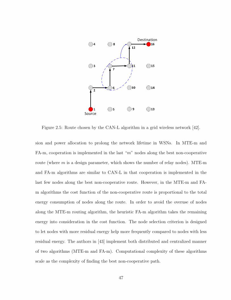
Figure 2.5: Route chosen by the CAN-L algorithm in a grid wireless network [42].

sion and power allocation to prolong the network lifetime in WSNs. In MTE-m and

FA-m, cooperation is implemented in the last “m” nodes along the best non-cooperative

route (where m is a design parameter, which shows the number of relay nodes). MTE-m

and FA-m algorithms are similar to CAN-L in that cooperation is implemented in the

last few nodes along the best non-cooperative route. However, in the MTE-m and FA-

m algorithms the cost function of the non-cooperative route is proportional to the total

energy consumption of nodes along the route. In order to avoid the overuse of nodes

along the MTE-m routing algorithm, the heuristic FA-m algorithm takes the remaining

energy into consideration in the cost function. The node selection criterion is designed

to let nodes with more residual energy help more frequently compared to nodes with less

residual energy. The authors in [43] implement both distributed and centralized manner

of two algorithms (MTE-m and FA-m). Computational complexity of these algorithms

scale as the complexity of finding the best non-cooperative path.

47

C. Cooperative Along Shortest Non-Cooperative Path (CASNCP) [34] applies coop-

erative communication to the shortest-path route in a distributed fashion to minimize the

total transmission power. The CASNCP algorithm first chooses the conventional shortest-

path route by employing the distributed Bellma−Ford shortest path algorithm [89]. Next,

for each three consecutive nodes in the route, the algorithm applies either the cooperative

transmission mode (where the first node is assigned to be the transmitter node, the second

node is assigned as the relay node, and the third node is assigned as the receiver node),

or the direct transmission mode from the transmitter to the receiver node. Therefore,

the algorithm is a sub-optimal one that belongs to the Cooperative Along Non-cooperative

Path category. The computational complexity of CASNCP is equal to the complexity of

running the Bellman-Ford algorithm, i.e., O(NM) (where N is the number of nodes and

M is the number of links in the network).

D. Throughput Optimized Cooperative Routing (TOCR) [59] is proposed to improve

the ad hoc network throughput by improving the throughput of each link with the help

of cooperative relay nodes. TOCR is based on the Adaptive Forwarding Cluster Routing

(AFCR) protocol [90]. In the AFCR protocol, nodes are divided into several 1-hop clusters

by a mobile clustering algorithm. In order to establish routes between cluster-heads in

adjacent clusters, local routing information is exchanged between neighboring nodes and

each node in the network has a neighbor table, namely the Cluster Membership (CM)

table. The CM table stores the cluster membership, and a routing table to store routes

to each cluster-head. When there are data packets to forward, the node first searches for

the destination node in its CM table and, if the destination node is in the table, it sends

the data packets to the destination node directly. Otherwise, it searches in the CM table

to find the cluster-head to which the destination node belongs. If the cluster head exists,

48

the node checks its routing table, and it sends the data packets to the next hop according

to the routing table. If there is no information about the destination node in the tables, it

buffers the incoming data packets and waits for building a route to the destination node.

As a result, a non-cooperative route is built from each node to the destination node. When

the non-cooperative route is built, each node of the selected route executes the following

steps to establish the cooperative link to the next hop node along the non-cooperative

path. Hence, TOCR is a sub-optimal cooperative routing and belongs to the Cooperative

Along Non-cooperative Path category. Each node calculates the throughput of the link to

its next hop node and the throughput gain of the cooperative link corresponding to each

potential cooperative relay. As shown in Fig. 2.4, the potential relay nodes are located

in the intersection of the coverage areas of the transmitter and the receiver nodes. The

throughput gains obtained by selecting each relay node are compared and the node that

leads to the maximum throughput gain is selected as the best relay node of that specific

link. The computational complexity of TOCR is mainly related to the AFCR construction

and the cooperation scheme slightly increases the complexity.

E. Cross-Layer Cooperative Routing (CLCR) [67] is the only cooperative routing pro-

posed for vehicular networks. Vehicular networks support vehicle-to-vehicle communica-

tions and hybrid architectures, which combines roadside units-to-vehicle and vehicle-to-

vehicle communication to support vehicular communications. However, since the move-

ments of vehicles is very fast, links between vehicle-to-vehicle or roadside units to ve-

hicle are unreliable and intermittent. CLCR is proposed to overcome the unreliability

of the wireless channel in vehicular networks and to maximize the system throughput

in a distributed fashion. In the CLCR algorithm, a routing protocol similar to Ad hoc

On-Demand Distance Vector (AODV) [91] is used to find a non-cooperative path and

49

then improves the performance using cooperative transmission; therefore, it employs Co-

operation Along Non-cooperative Path which is a sub-optimal cooperative routing. In the

considered scenario shown in Fig. 2.6, every vehicle is under the radio coverage of a road-

side unit, and vehicles periodically exchange Hello packets with their one hop neighbors to

know each others speeds, positions, and directions. Furthermore, roadside units exchange

information and synchronize their information using a fixed reliable roadside unit. When

the source vehicle has packet to send, it only needs to know the destination vehicle ID. As

in AODV, when a source vehicle needs a path to a destination node, the source initiates a

route discovery process by generating a route-request packet and then waits for a route-

reply. If the destination node receives the route-request packet, it sends a route-reply to

the source vehicle along the route travelled by the received route-request packet but in the

reverse direction, and therefore, the non-cooperative path is found. Two algorithms are

proposed to select the most appropriate relay nodes. In the first algorithm, the holding

time of a connection between the transmitter and potential relay nodes, and between the

receiver and potential relay node are predicted in order to select the most appropriate

relay node. Therefore, the relay node selection is based on the duration during which the

potential relay node stays connected to the transmitter and receiver nodes. The relay

node should be connected to the receiver and the transmitter nodes as long as possible

to achieve the benefit of cooperative transmission and to avoid the overhead caused by

frequent relay node reselection. In the second algorithm, the cost of each potential relay

node is calculated and the node with the minimum cost (that has the maximum holding

connected time and the maximum throughput) is deemed the best choice of the relay

node. In this algorithm, the selection of a relay node significantly affects the performance

of CLCR.

50

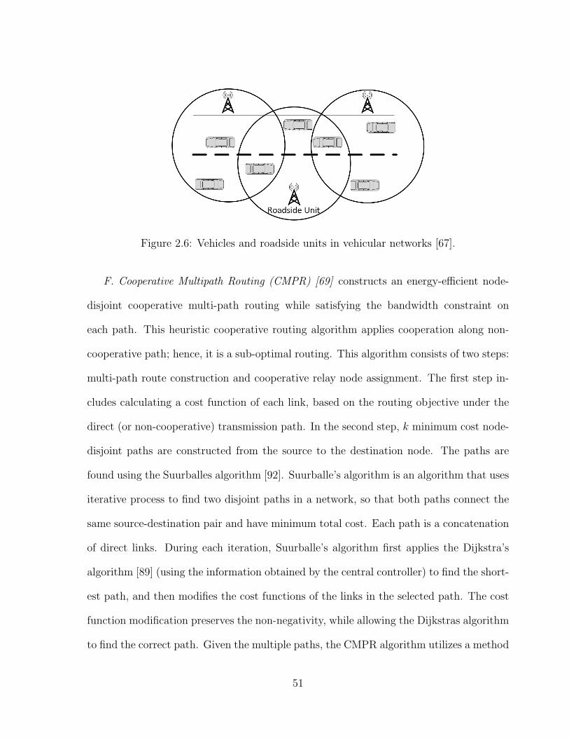
Figure 2.6: Vehicles and roadside units in vehicular networks [67].

F. Cooperative Multipath Routing (CMPR) [69] constructs an energy-efficient node-

disjoint cooperative multi-path routing while satisfying the bandwidth constraint on

each path. This heuristic cooperative routing algorithm applies cooperation along non-

cooperative path; hence, it is a sub-optimal routing. This algorithm consists of two steps:

multi-path route construction and cooperative relay node assignment. The first step in-

cludes calculating a cost function of each link, based on the routing objective under the

direct (or non-cooperative) transmission path. In the second step, k minimum cost node-

disjoint paths are constructed from the source to the destination node. The paths are

found using the Suurballes algorithm [92]. Suurballe’s algorithm is an algorithm that uses

iterative process to find two disjoint paths in a network, so that both paths connect the

same source-destination pair and have minimum total cost. Each path is a concatenation

of direct links. During each iteration, Suurballe’s algorithm first applies the Dijkstra’s

algorithm [89] (using the information obtained by the central controller) to find the short-

est path, and then modifies the cost functions of the links in the selected path. The cost

function modification preserves the non-negativity, while allowing the Dijkstras algorithm

to find the correct path. Given the multiple paths, the CMPR algorithm utilizes a method

51

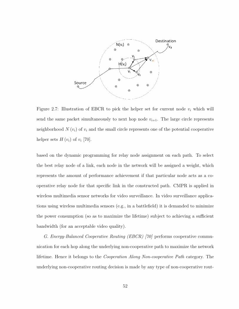
Figure 2.7: Illustration of EBCR to pick the helper set for current node vi which will

send the same packet simultaneously to next hop node vi+1. The large circle represents

neighborhood N (vi) of vi and the small circle represents one of the potential cooperative

helper sets H (vi) of vi [70].

based on the dynamic programming for relay node assignment on each path. To select

the best relay node of a link, each node in the network will be assigned a weight, which

represents the amount of performance achievement if that particular node acts as a co-

operative relay node for that specific link in the constructed path. CMPR is applied in

wireless multimedia sensor networks for video surveillance. In video surveillance applica-

tions using wireless multimedia sensors (e.g., in a battlefield) it is demanded to minimize

the power consumption (so as to maximize the lifetime) subject to achieving a sufficient

bandwidth (for an acceptable video quality).

G. Energy-Balanced Cooperative Routing (EBCR) [70] performs cooperative commu-

nication for each hop along the underlying non-cooperative path to maximize the network

lifetime. Hence it belongs to the Cooperation Along Non-cooperative Path category. The

underlying non-cooperative routing decision is made by any type of non-cooperative rout-

52

ing strategy, such as energy-efficient ad hoc routing protocol or shortest path based routing

algorithms. In order to apply cooperative communication to each link, as illustrated in

Fig. 2.7, a relay set for each transmitter node along the path is selected using the fol-

lowing steps. Firstly, a potential relay set is defined as any neighbors of the transmitter

node that are closer to the transmitter than the receiver node. Given a potential relay

set with size k, the remaining lifetimes of the transmitter node and its relay set (under

cooperative communication model) are calculated. Then, all of these k + 1 nodes are

sorted in a descending order by their remaining lifetime. Finally, the algorithm greedily

picks those nodes with a longer remaining lifetime and uses them as the relay nodes until

the cumulative signal strength at the receiver node is greater than or equal to a detection

threshold, i.e, until the received signal strength meets the detection requirement. In this

algorithm a central controller is required to collect the potential relay set and pick the

best relay nodes to prolong the network lifetime.

H. Minimum Power Cooperative Routing (MPCR) [34] minimizes the transmission

power using cooperative routing in a distributed manner. MPCR exploits cooperative

communication while constructing a minimum-power route; therefore, it is a cooperative-

based routing algorithm. In the MPCR algorithm, first, each node calculates the cost of

connection to each of its neighbor either in the cooperative mode (by employing all poten-

tial single-relay nodes) or the direct mode. Second, the algorithm applies the distributed

shortest path Bellman-Ford algorithm to select the minimum cost route using the calcu-

lated costs. To obtain the best relay node in the cooperative mode of the first phase, the

algorithm investigates all possible relay nodes in the transmitter node’s neighborhood and

if the minimum cost (transmission power) corresponds to a specific relay node, that node

is selected to cooperate. If there is no available relay node in the neighborhood, a direct

53

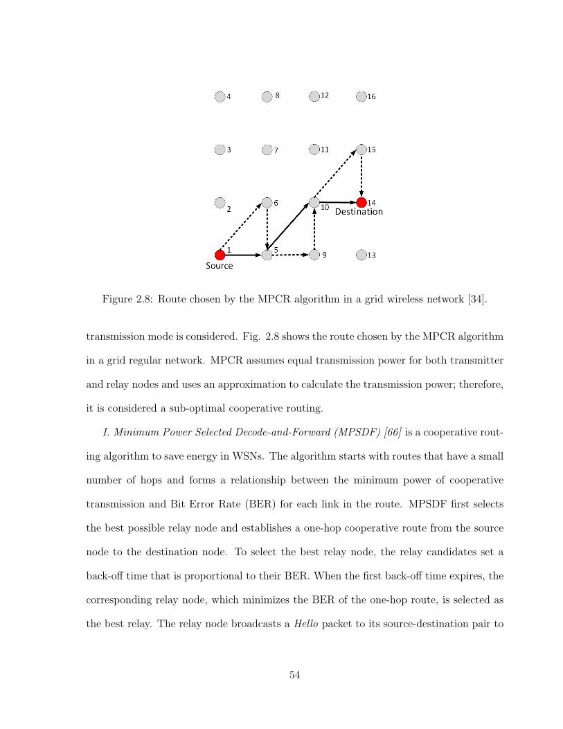
Figure 2.8: Route chosen by the MPCR algorithm in a grid wireless network [34].

transmission mode is considered. Fig. 2.8 shows the route chosen by the MPCR algorithm

in a grid regular network. MPCR assumes equal transmission power for both transmitter

and relay nodes and uses an approximation to calculate the transmission power; therefore,

it is considered a sub-optimal cooperative routing.

I. Minimum Power Selected Decode-and-Forward (MPSDF) [66] is a cooperative rout-

ing algorithm to save energy in WSNs. The algorithm starts with routes that have a small

number of hops and forms a relationship between the minimum power of cooperative

transmission and Bit Error Rate (BER) for each link in the route. MPSDF first selects

the best possible relay node and establishes a one-hop cooperative route from the source

node to the destination node. To select the best relay node, the relay candidates set a

back-off time that is proportional to their BER. When the first back-off time expires, the

corresponding relay node, which minimizes the BER of the one-hop route, is selected as

the best relay. The relay node broadcasts a Hello packet to its source-destination pair to

54

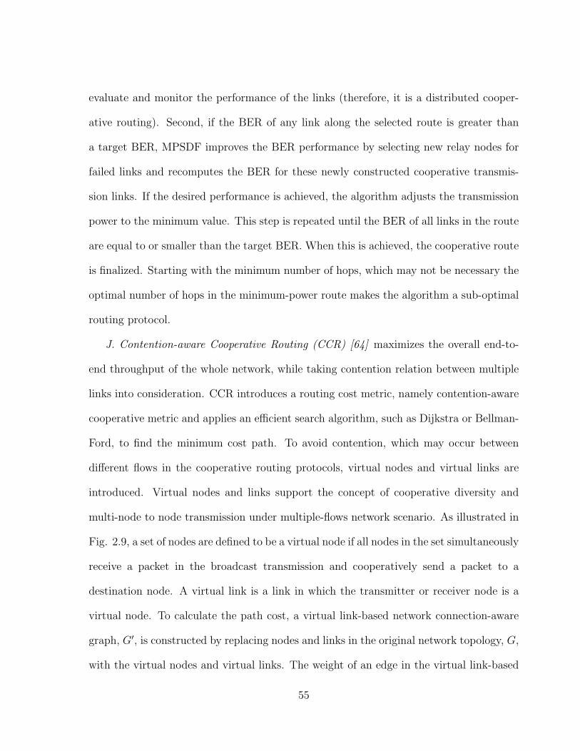
evaluate and monitor the performance of the links (therefore, it is a distributed cooper-

ative routing). Second, if the BER of any link along the selected route is greater than

a target BER, MPSDF improves the BER performance by selecting new relay nodes for

failed links and recomputes the BER for these newly constructed cooperative transmis-

sion links. If the desired performance is achieved, the algorithm adjusts the transmission

power to the minimum value. This step is repeated until the BER of all links in the route

are equal to or smaller than the target BER. When this is achieved, the cooperative route

is finalized. Starting with the minimum number of hops, which may not be necessary the

optimal number of hops in the minimum-power route makes the algorithm a sub-optimal

routing protocol.

J. Contention-aware Cooperative Routing (CCR) [64] maximizes the overall end-to-

end throughput of the whole network, while taking contention relation between multiple

links into consideration. CCR introduces a routing cost metric, namely contention-aware

cooperative metric and applies an efficient search algorithm, such as Dijkstra or Bellman-

Ford, to find the minimum cost path. To avoid contention, which may occur between

different flows in the cooperative routing protocols, virtual nodes and virtual links are

introduced. Virtual nodes and links support the concept of cooperative diversity and

multi-node to node transmission under multiple-flows network scenario. As illustrated in

Fig. 2.9, a set of nodes are defined to be a virtual node if all nodes in the set simultaneously

receive a packet in the broadcast transmission and cooperatively send a packet to a

destination node. A virtual link is a link in which the transmitter or receiver node is a

virtual node. To calculate the path cost, a virtual link-based network connection-aware

graph, G′, is constructed by replacing nodes and links in the original network topology, G,

with the virtual nodes and virtual links. The weight of an edge in the virtual link-based

55

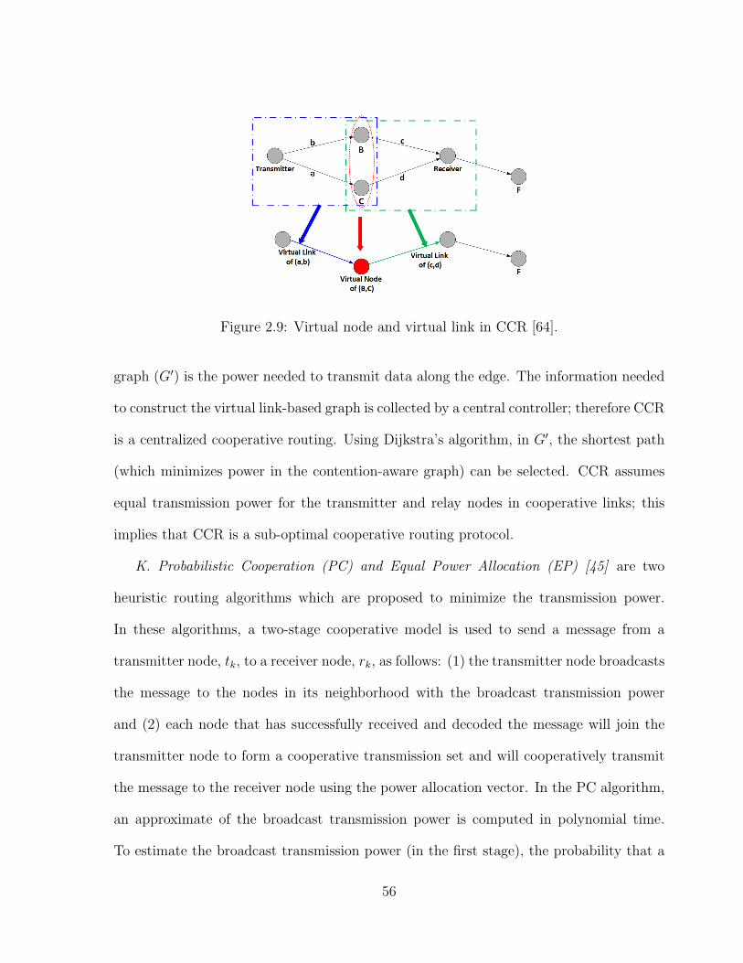
Figure 2.9: Virtual node and virtual link in CCR [64].

graph (G′) is the power needed to transmit data along the edge. The information needed

to construct the virtual link-based graph is collected by a central controller; therefore CCR

is a centralized cooperative routing. Using Dijkstra’s algorithm, in G′, the shortest path

(which minimizes power in the contention-aware graph) can be selected. CCR assumes

equal transmission power for the transmitter and relay nodes in cooperative links; this

implies that CCR is a sub-optimal cooperative routing protocol.

K. Probabilistic Cooperation (PC) and Equal Power Allocation (EP) [45] are two

heuristic routing algorithms which are proposed to minimize the transmission power.

In these algorithms, a two-stage cooperative model is used to send a message from a

transmitter node, tk, to a receiver node, rk, as follows: (1) the transmitter node broadcasts

the message to the nodes in its neighborhood with the broadcast transmission power

and (2) each node that has successfully received and decoded the message will join the

transmitter node to form a cooperative transmission set and will cooperatively transmit

the message to the receiver node using the power allocation vector. In the PC algorithm,

an approximate of the broadcast transmission power is computed in polynomial time.

To estimate the broadcast transmission power (in the first stage), the probability that a

56

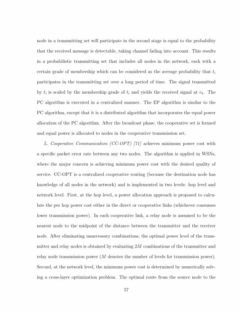
node in a transmitting set will participate in the second stage is equal to the probability

that the received message is detectable, taking channel fading into account. This results

in a probabilistic transmitting set that includes all nodes in the network, each with a

certain grade of membership which can be considered as the average probability that ti

participates in the transmitting set over a long period of time. The signal transmitted

by ti is scaled by the membership grade of ti and yields the received signal at rk. The

PC algorithm is executed in a centralized manner. The EP algorithm is similar to the

PC algorithm, except that it is a distributed algorithm that incorporates the equal power

allocation of the PC algorithm. After the broadcast phase, the cooperative set is formed

and equal power is allocated to nodes in the cooperative transmission set.

L. Cooperative Communication (CC-OPT) [71] achieves minimum power cost with

a specific packet error rate between any two nodes. The algorithm is applied in WSNs,

where the major concern is achieving minimum power cost with the desired quality of

service. CC-OPT is a centralized cooperative routing (because the destination node has

knowledge of all nodes in the network) and is implemented in two levels: hop level and

network level. First, at the hop level, a power allocation approach is proposed to calcu-

late the per hop power cost either in the direct or cooperative links (whichever consumes

lower transmission power). In each cooperative link, a relay node is assumed to be the

nearest node to the midpoint of the distance between the transmitter and the receiver

node. After eliminating unnecessary combinations, the optimal power level of the trans-

mitter and relay nodes is obtained by evaluating 2M combinations of the transmitter and

relay node transmission power (M denotes the number of levels for transmission power).

Second, at the network level, the minimum power cost is determined by numerically solv-

ing a cross-layer optimization problem. The optimal route from the source node to the

57

Figure 2.10: Wireless mesh network of base stations [37].

destination node is a combination of multiple direct communication hops and cooperative

communication hops. Due to assigning the relay node as the nearest node to the middle

point and assuming constant transmission power, CC-OPT is a sub-optimal cooperative

routing algorithm.

M. Power Aware Cooperative Routing (PACR) [37] is a distributed cooperative routing

that takes the active radio electronic power into account while constructing the route that

consumes minimum-power to transmit a message from a source to its destination node.

PACR is mainly proposed for cooperative routing in cellular wireless mesh networks. The

algorithm is applied to a wireless mesh network consisting of a large number of cellular

base stations (BS) and each BS has a single omnidirectional antenna. Fig. 2.10 shows

this scenario where a source BS sends data to a destination BS and the algorithm finds a

cooperative route between source and the destination with minimum power consumption.

In this algorithm, a source node selects its l neighboring nodes, but it does not transfer

58

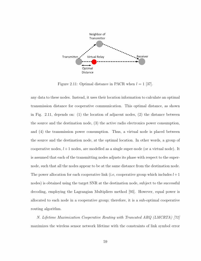
Figure 2.11: Optimal distance in PACR when l = 1 [37].

any data to these nodes. Instead, it uses their location information to calculate an optimal

transmission distance for cooperative communication. This optimal distance, as shown

in Fig. 2.11, depends on: (1) the location of adjacent nodes, (2) the distance between

the source and the destination node, (3) the active radio electronics power consumption,

and (4) the transmission power consumption. Thus, a virtual node is placed between

the source and the destination node, at the optimal location. In other words, a group of

cooperative nodes, l+ 1 nodes, are modelled as a single super-node (or a virtual node). It

is assumed that each of the transmitting nodes adjusts its phase with respect to the super-

node, such that all the nodes appear to be at the same distance from the destination node.

The power allocation for each cooperative link (i.e, cooperative group which includes l+1

nodes) is obtained using the target SNR at the destination node, subject to the successful

decoding, employing the Lagrangian Multipliers method [93]. However, equal power is

allocated to each node in a cooperative group; therefore, it is a sub-optimal cooperative

routing algorithm.

N. Lifetime Maximization Cooperative Routing with Truncated ARQ (LMCRTA) [72]

maximizes the wireless sensor network lifetime with the constraints of link symbol error

59

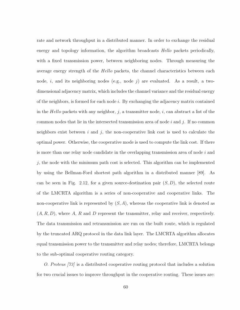
rate and network throughput in a distributed manner. In order to exchange the residual

energy and topology information, the algorithm broadcasts Hello packets periodically,

with a fixed transmission power, between neighboring nodes. Through measuring the

average energy strength of the Hello packets, the channel characteristics between each

node, i, and its neighboring nodes (e.g., node j) are evaluated. As a result, a two-

dimensional adjacency matrix, which includes the channel variance and the residual energy

of the neighbors, is formed for each node i. By exchanging the adjacency matrix contained

in the Hello packets with any neighbor, j, a transmitter node, i, can abstract a list of the

common nodes that lie in the intersected transmission area of node i and j. If no common

neighbors exist between i and j, the non-cooperative link cost is used to calculate the

optimal power. Otherwise, the cooperative mode is used to compute the link cost. If there

is more than one relay node candidate in the overlapping transmission area of node i and

j, the node with the minimum path cost is selected. This algorithm can be implemented

by using the Bellman-Ford shortest path algorithm in a distributed manner [89]. As

can be seen in Fig. 2.12, for a given source-destination pair (S,D), the selected route

of the LMCRTA algorithm is a series of non-cooperative and cooperative links. The

non-cooperative link is represented by (S,A), whereas the cooperative link is denoted as

(A,R,D), where A, R and D represent the transmitter, relay and receiver, respectively.

The data transmission and retransmission are run on the built route, which is regulated

by the truncated ARQ protocol in the data link layer. The LMCRTA algorithm allocates

equal transmission power to the transmitter and relay nodes; therefore, LMCRTA belongs

to the sub-optimal cooperative routing category.

O. Proteus [73] is a distributed cooperative routing protocol that includes a solution

for two crucial issues to improve throughput in the cooperative routing. These issues are:

60

(1) the number of cooperative transmitter nodes for each link and (2) the cooperative

strategy used by the transmitter nodes. This algorithm is divided into three steps for the

route discovery phase. In the first step, a Route Request (RREQ) packet is transmitted by

the source node. Similar to the route request packets in conventional routing (e.g., [94]),

nodes stamp their IDs on the RREQ packets. In addition to the ID, each node stamps

the following information on the RREQ packets: (a) the received signal strength from

the previous hop, (b) the neighboring list containing the number of links overheard by

each neighboring node, (c) the ambient interference level (determined by the duration of

time that the channel is busy), and (d) the number of flows that are already served by

the node. The second step involves the route response; once the destination node receives

the route request, it transmits the Route Response Packet (RREP) after attaching the

information about its neighbor nodes. Intermediate nodes forward the packet as usual;

however, when any of their statistics change, they adjust it on the route response packet.

In the third step, once the source receives the route response, it uses the statistics available

in the packet to obtain the routing throughput. Within a time-out duration, the source

node gathers the received information of k paths, where k is a predetermined constant.

The source calculates the path throughput metric for a different number of cooperative

transmitter nodes (relay nodes) and for different cooperative schemes, and then selects

the route with the best metric. In the Proteus algorithm, the fixed equal transmission

power is allocated to nodes along cooperative route (either relay or transmitter node);

therefore, it is not optimal cooperative routing. Moreover, the algorithm only focuses on

the route-discovery step of the routing protocol. Other components such as forwarding

are similar to the Dynamic Source Routing protocol (DSR) [95], which is an on-demand

routing protocol. However, the source route packet consists of the number of relay nodes

61

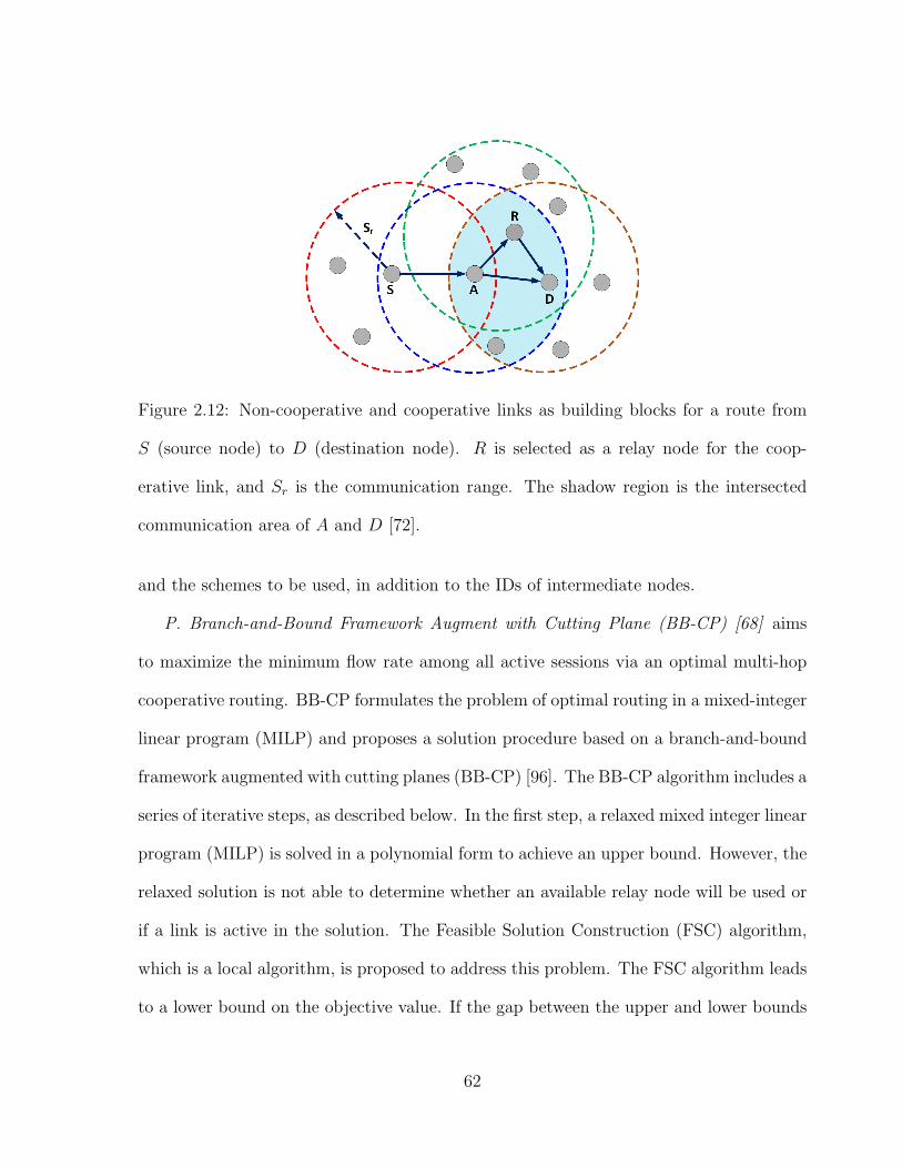
Figure 2.12: Non-cooperative and cooperative links as building blocks for a route from

S (source node) to D (destination node). R is selected as a relay node for the coop-

erative link, and Sr is the communication range. The shadow region is the intersected

communication area of A and D [72].

and the schemes to be used, in addition to the IDs of intermediate nodes.

P. Branch-and-Bound Framework Augment with Cutting Plane (BB-CP) [68] aims

to maximize the minimum flow rate among all active sessions via an optimal multi-hop

cooperative routing. BB-CP formulates the problem of optimal routing in a mixed-integer

linear program (MILP) and proposes a solution procedure based on a branch-and-bound

framework augmented with cutting planes (BB-CP) [96]. The BB-CP algorithm includes a

series of iterative steps, as described below. In the first step, a relaxed mixed integer linear

program (MILP) is solved in a polynomial form to achieve an upper bound. However, the

relaxed solution is not able to determine whether an available relay node will be used or

if a link is active in the solution. The Feasible Solution Construction (FSC) algorithm,

which is a local algorithm, is proposed to address this problem. The FSC algorithm leads

to a lower bound on the objective value. If the gap between the upper and lower bounds

62

is greater than a predetermined value, ε, linear constraints, namely cutting planes, will be

added and the relaxed linear programming will be solved again. Cutting planes improve

the values of the upper and lower bounds, reducing the feasible region of the relaxed

problem. Then, the improved upper bounding solution that is obtained from this relaxed

solution is used in the local FSC algorithm to achieve a new feasible (possibly improved)

lower bounding solution. A number of cutting planes are added to the relaxed problem

until the improvements (of upper and lower bound) are within the certain percentage of

threshold, i.e, further improvement in upper and lower bounds becomes marginal. When

this certain threshold is met, adding more cutting planes does not improve the bounds

and the problem is partitioned into two sub-problems. As the last step of the iteration,

the relaxed versions of the two sub-problems are solved and the upper and lower bounds

for each sub-problem are obtained using the FSC algorithm. After each iteration, if

the gap between the largest upper bound and the largest lower bounds (among all the

sub-problems) is greater than ε, a similar iterative step is performed on the sub-problem

having the largest upper bound. After each iteration, the total number of sub-problems is

increased because the chosen sub-problem is partitioned into two sub-problems. BB-CP

presents the optimal cooperative routing techniques based on the centralized approach.

Q. Energy Efficient Cooperative Routing in Wireless Sensor Networks [63], which we

call EECRWSN in this paper, is designed to minimize the total energy consumption in

the WSNs. This work proposes a framework for formulation of the optimal relay node

selection and power allocation, which leads to a mixed integer linear programming prob-

lem. The binary variables are used in this framework to re-express the logical statements

as linear relations which contain both linear and binary variables. For instance, binary

variable δk is used for each neighboring node, k, to show whether the received signal in

63

the neighboring node is greater than prescribed threshold. If the condition is met, i.e.,

this node will be engaged in cooperative transmission, then δk = 1; otherwise, δk = 0.

The required computational complexity of the algorithm to solve these problems grows

exponentially with the number of binary variables; therefore, it may be prohibitive to

implement it on the simple hardware utilized in wireless sensor networks. In order to

solve this problem, the multi-parametric programming is invoked [97]. Through the use

of multi-parametric programming techniques the infinite size problem is decomposed into

a number of finite size problems. Multi-parametric programming makes the proposed

strategy a low-complexity implementation method. The low-complexity implementation

method obtains a solution as a function of the parameters of the network. This solution

is calculated off-line, and is saved on the memory chip of every sensing node; therefore,

the on-line computation is reduced to the evaluation of the parametric functions. In this

work, the optimal routing is obtained and it is shown that for a specific configuration,

the proposed framework selects the best set of relaying nodes, as well as the optimal

transmission power for broadcasting and cooperative transmission.

2.9 Performance and Challenges of Cooperative Rout-

ing

Table 2.1 compares some of the most significant cooperative routing algorithms according

to the taxonomy we described in Section 2.4. It is clear from Table 2.1 that most of

the proposed algorithms are sub-optimal. Sub-optimal cooperative routing algorithms

are simpler to obtain, while their performance is slightly lower than the optimal one (as

64

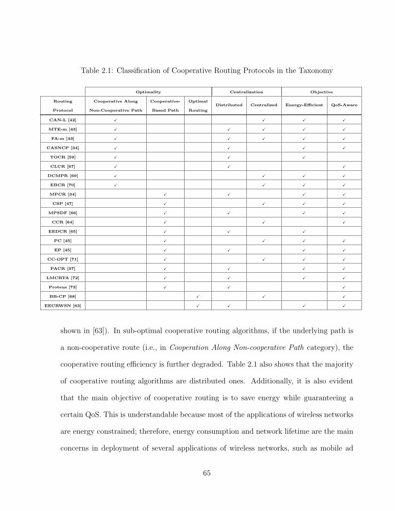
Table 2.1: Classification of Cooperative Routing Protocols in the Taxonomy

Optimality Centralization Objective

Routing

Protocol

Cooperative Along

Non-Cooperative Path

Cooperative-

Based Path

Optimal

Routing

Distributed Centralized Energy-Efficient QoS-Aware

CAN-L [42] X X X X

MTE-m [43] X X X X X

FA-m [43] X X X X X

CASNCP [34] X X X X

TOCR [59] X X X

CLCR [67] X X X

DCMPR [69] X X X X

EBCR [70] X X X X

MPCR [34] X X X X

CSP [47] X X X X

MPSDF [66] X X X X

CCR [64] X X X

EEDCR [65] X X X

PC [45] X X X X

EP [45] X X X X

CC-OPT [71] X X X X

PACR [37] X X X X

LMCRTA [72] X X X X

Proteus [73] X X X

BB-CP [68] X X X

EECRWSN [63] X X X X

shown in [63]). In sub-optimal cooperative routing algorithms, if the underlying path is

a non-cooperative route (i.e., in Cooperation Along Non-cooperative Path category), the

cooperative routing efficiency is further degraded. Table 2.1 also shows that the majority

of cooperative routing algorithms are distributed ones. Additionally, it is also evident

that the main objective of cooperative routing is to save energy while guaranteeing a

certain QoS. This is understandable because most of the applications of wireless networks

are energy constrained; therefore, energy consumption and network lifetime are the main

concerns in deployment of several applications of wireless networks, such as mobile ad

65

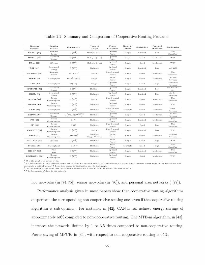
Table 2.2: Summary and Comparison of Cooperative Routing Protocols

Routing

Protocol

Routing

MetricComplexity

Num. of

Relays

Power

Allocation

Num. of

FlowsScalability

Protocol

OverheadApplication

CAN-L [42]Required

PowerO

(N2

)Multiple (= L)

Optimal

PowerSingle Limited Low

Not

Specified

MTE-m [43]Consumed

EnergyO

(N2

)Multiple (= m)

Optimal

PowerSingle Good Moderate WSN

FA-m [43] Lifetime O(N2

)Multiple (= m)

Optimal


CSP [47]Consumed

EnergyO

(N2

)Multiple

Optimal

PowerSingle Limited Low All WN

CASNCP [34]Required

PowerO (NM)1 Single

Sub-Optimal

PowerSingle Good Moderate

Not

Specified

TOCR [59] Throughput O(N2logN

)Single

Equal


Ad hoc

Network

CLCR [67] Throughput O (2N) SingleOptimal

PowerSingle Good High

Vehicular

Network

DCMPR [69]Consumed

EnergyO

(N3

)Multiple

Optimal


Multimedia

SN

EBCR [70]Consumed

EnergyO

(N3

)Multiple

Optimal


Ad hoc

Network

MPCR [34]Power

ConsumptionO

(N3

)Single

Sub-Optimal


Not

Specified

MPSDF [66]Power

ConsumptionO

(N2

)Multiple

Optimal


CCR [64] Throughput O(N2

)Multiple

Sub-Optimal

PowerMultiple Good Moderate

Mesh

Network

EEDCR [65]Consumed

EnergyO

(N∆(h)2∆(h)

)2 Multiple

Optimal


Ad hoc

Network

PC [45]Power

ConsumptionO (N) Multiple

Optimal

PowerSingle Limited Moderate

Not

Specified

EP [45]Power

ConsumptionO (1) Multiple

Sub-Optimal

PowerSingle Good Low

Not

Specified

CC-OPT [71]Power

ConsumptionO

(N3

)Single

Sub-Optimal

PowerSingle Limited Low WSN

PACR [37]Power

ConsumptionO (Nl)3

Multiple

(Single Virtual)

Equal


Cellular

Network

LMCRTA [72] Lifetime O(N2

)Multiple

Equal

PowerSingle Good High WSN

Proteus [73] Throughput O (F )4 MultipleEqual

PowerMultiple Good High

Not

Specified

BB-CP [68]Flow

RateO

(2N

)Multiple

Optimal

PowerSingle Limited Moderate

Not

Specified

EECRWSN [63]Energy

ConsumptionO

(2N

)Multiple

Optimal


1 M is the number of power levels.2 h is the number of hops between source and the destination node and ∆ (h) is the degree of a graph which connects source node to the destination node

and exists a path of at most h hops from source to destination node in that graph.3 l is the number of neighbors that their location information is used to find the optimal distance in PACR.4 F is the number of flows in the network.

hoc networks (in [74,75]), sensor networks (in [76]), and personal area networks ( [77]).

Performance analysis given in most papers show that cooperative routing algorithms

outperform the corresponding non-cooperative routing ones even if the cooperative routing

algorithm is sub-optimal. For instance, in [42], CAN-L can achieve energy savings of

approximately 50% compared to non-cooperative routing. The MTE-m algorithm, in [43],

increases the network lifetime by 1 to 3.5 times compared to non-cooperative routing.

Power saving of MPCR, in [34], with respect to non-cooperative routing is 65%.

66

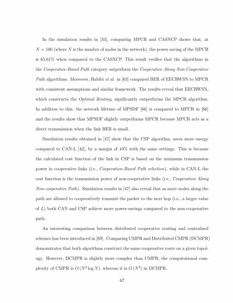
In the simulation results in [34], comparing MPCR and CASNCP shows that, at

N = 100 (where N is the number of nodes in the network), the power saving of the MPCR

is 65.61% when compared to the CASNCP. This result verifies that the algorithms in

the Cooperative-Based Path category outperform the Cooperative Along Non-Cooperative

Path algorithms. Moreover, Habibi et al. in [63] compared BER of EECRWSN to MPCR

with consistent assumptions and similar framework. The results reveal that EECRWSN,

which constructs the Optimal Routing, significantly outperforms the MPCR algorithm.

In addition to this, the network lifetime of MPSDF [66] is compared to MPCR in [66]

and the results show that MPSDF slightly outperforms MPCR because MPCR acts as a

direct transmission when the link BER is small.

Simulation results obtained in [47] show that the CSP algorithm, saves more energy

compared to CAN-L [42], by a margin of 10% with the same settings. This is because

the calculated cost function of the link in CSP is based on the minimum transmission

power in cooperative links (i.e., Cooperation-Based Path selection), while in CAN-L the

cost function is the transmission power of non-cooperative links (i.e., Cooperation Along

Non-cooperative Path). Simulation results in [47] also reveal that as more nodes along the

path are allowed to cooperatively transmit the packet to the next hop (i.e., a larger value

of L) both CAN and CSP achieve more power-savings compared to the non-cooperative

path.

An interesting comparison between distributed cooperative routing and centralized

schemes has been introduced in [69]. Comparing CMPR and Distributed CMPR (DCMPR)

demonstrates that both algorithms construct the same cooperative route on a given topol-

ogy. However, DCMPR is slightly more complex than CMPR; the computational com-

plexity of CMPR is O (N2 logN), whereas it is O (N3) in DCMPR.

67

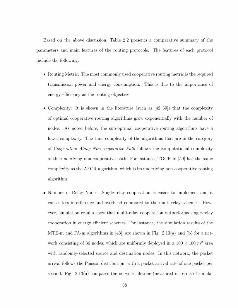
Based on the above discussion, Table 2.2 presents a comparative summary of the

parameters and main features of the routing protocols. The features of each protocol

include the following:

Routing Metric: The most commonly used cooperative routing metric is the required

transmission power and energy consumption. This is due to the importance of

energy efficiency as the routing objective.

Complexity: It is shown in the literature (such as [42, 69]) that the complexity

of optimal cooperative routing algorithms grow exponentially with the number of

nodes. As noted before, the sub-optimal cooperative routing algorithms have a

lower complexity. The time complexity of the algorithms that are in the category

of Cooperation Along Non-cooperative Path follows the computational complexity

of the underlying non-cooperative path. For instance, TOCR in [59] has the same

complexity as the AFCR algorithm, which is its underlying non-cooperative routing

algorithm.

Number of Relay Nodes: Single-relay cooperation is easier to implement and it

causes less interference and overhead compared to the multi-relay schemes. How-

ever, simulation results show that multi-relay cooperation outperforms single-relay

cooperation in energy efficient schemes. For instance, the simulation results of the

MTE-m and FA-m algorithms in [43], are shown in Fig. 2.13(a) and (b) for a net-

work consisting of 36 nodes, which are uniformly deployed in a 100 × 100 m2 area

with randomly-selected source and destination nodes. In this network, the packet

arrival follows the Poisson distribution, with a packet arrival rate of one packet per

second. Fig. 2.13(a) compares the network lifetime (measured in terms of simula-

68

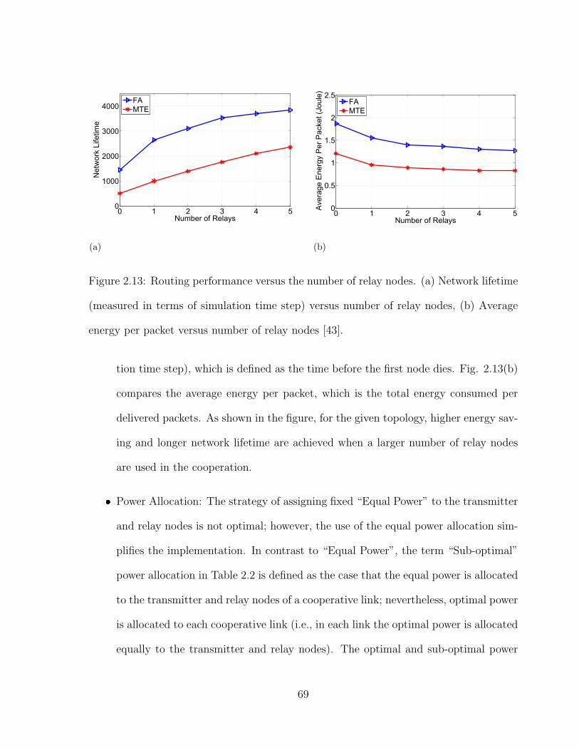
(a)

0 1 2 3 4 50

1000

2000

3000

4000

Number of Relays

Net

wor

k Li

fetim

e

FAMTE

(b)

0 1 2 3 4 50

0.5

1

1.5

2

2.5

Number of Relays

Aver

age

Ener

gy P

er P

acke

t (Jo

ule)

FAMTE

Figure 2.13: Routing performance versus the number of relay nodes. (a) Network lifetime

(measured in terms of simulation time step) versus number of relay nodes, (b) Average

energy per packet versus number of relay nodes [43].

tion time step), which is defined as the time before the first node dies. Fig. 2.13(b)

compares the average energy per packet, which is the total energy consumed per

delivered packets. As shown in the figure, for the given topology, higher energy sav-

ing and longer network lifetime are achieved when a larger number of relay nodes

are used in the cooperation.

Power Allocation: The strategy of assigning fixed “Equal Power” to the transmitter

and relay nodes is not optimal; however, the use of the equal power allocation sim-

plifies the implementation. In contrast to “Equal Power”, the term “Sub-optimal”

power allocation in Table 2.2 is defined as the case that the equal power is allocated

to the transmitter and relay nodes of a cooperative link; nevertheless, optimal power

is allocated to each cooperative link (i.e., in each link the optimal power is allocated

equally to the transmitter and relay nodes). The optimal and sub-optimal power

69

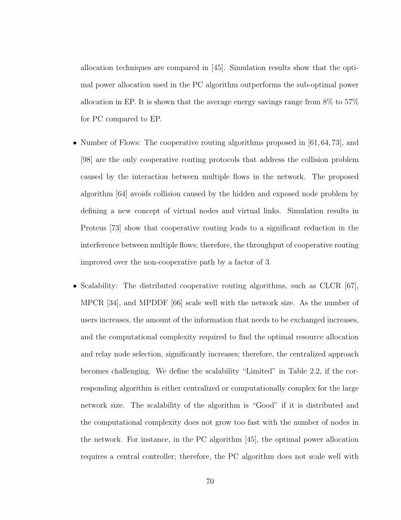
allocation techniques are compared in [45]. Simulation results show that the opti-

mal power allocation used in the PC algorithm outperforms the sub-optimal power

allocation in EP. It is shown that the average energy savings range from 8% to 57%

for PC compared to EP.

Number of Flows: The cooperative routing algorithms proposed in [61, 64, 73], and

[98] are the only cooperative routing protocols that address the collision problem

caused by the interaction between multiple flows in the network. The proposed

algorithm [64] avoids collision caused by the hidden and exposed node problem by

defining a new concept of virtual nodes and virtual links. Simulation results in

Proteus [73] show that cooperative routing leads to a significant reduction in the

interference between multiple flows; therefore, the throughput of cooperative routing

improved over the non-cooperative path by a factor of 3.

Scalability: The distributed cooperative routing algorithms, such as CLCR [67],

MPCR [34], and MPDDF [66] scale well with the network size. As the number of

users increases, the amount of the information that needs to be exchanged increases,

and the computational complexity required to find the optimal resource allocation

and relay node selection, significantly increases; therefore, the centralized approach

becomes challenging. We define the scalability “Limited” in Table 2.2, if the cor-

responding algorithm is either centralized or computationally complex for the large

network size. The scalability of the algorithm is “Good” if it is distributed and

the computational complexity does not grow too fast with the number of nodes in

the network. For instance, in the PC algorithm [45], the optimal power allocation

requires a central controller; therefore, the PC algorithm does not scale well with

70

the network size. In contrast to the PC algorithm, the EP algorithm (also in [45])

is proposed with the equal power allocation; hence, EP is a distributed algorithm

and scales well with the network size.

Protocol Overhead: Dealing with the overhead caused by controlling messages for

relay selection, channel estimation, power allocation, and route selection is chal-

lenging in cooperative routing algorithms. We define overhead as “High” if the

corresponding algorithm has a large number of controlling messages and involves

frequent refreshing. Overhead is defined as “Medium” if the algorithm has a large

number of control messages and does not require refreshing frequently. Overhead is

defined as “Low” if the algorithm has a limited number of controlling messages which

rarely get updated. Simulation results in [72] show that the overhead of LMCRTA

is higher than that of the MTE-m and FA-m in [43], with the same throughput

requirement. Moreover, in CLCR [67], which is a cooperative routing algorithm

for vehicular networks, the dynamic features of the network cause overhead by fre-

quent relay node reselection. In other words, in CLCR, the routing overhead is

incurred to keep the relay nodes connected or to reselect the best relay nodes in

each transmission time.

Applications: The main application of cooperative routing is in power-limited net-

works, such as WSNs and ad hoc networks, because energy saving is the main

objective of cooperative routing in the literature, such as [66]. Cooperative routing

is also applied to vehicular networks in [67] to overcome the unreliability of the

wireless channels and to maximize the system throughput.

In the following subsections, we present the most dominant and important factors

71

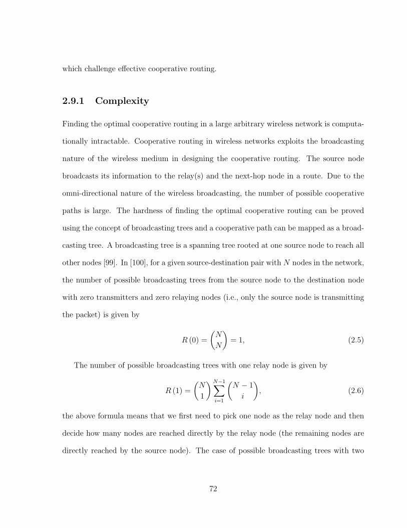
which challenge effective cooperative routing.

2.9.1 Complexity

Finding the optimal cooperative routing in a large arbitrary wireless network is computa-

tionally intractable. Cooperative routing in wireless networks exploits the broadcasting

nature of the wireless medium in designing the cooperative routing. The source node

broadcasts its information to the relay(s) and the next-hop node in a route. Due to the

omni-directional nature of the wireless broadcasting, the number of possible cooperative

paths is large. The hardness of finding the optimal cooperative routing can be proved

using the concept of broadcasting trees and a cooperative path can be mapped as a broad-

casting tree. A broadcasting tree is a spanning tree rooted at one source node to reach all

other nodes [99]. In [100], for a given source-destination pair with N nodes in the network,

the number of possible broadcasting trees from the source node to the destination node

with zero transmitters and zero relaying nodes (i.e., only the source node is transmitting

the packet) is given by

R (0) =

(N

N

)= 1, (2.5)

The number of possible broadcasting trees with one relay node is given by

R (1) =

(N

1

)N−1∑i=1

(N − 1

i

), (2.6)

the above formula means that we first need to pick one node as the relay node and then

decide how many nodes are reached directly by the relay node (the remaining nodes are

directly reached by the source node). The case of possible broadcasting trees with two

72

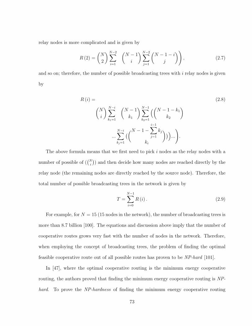
relay nodes is more complicated and is given by

R (2) =

(N

2

)N−2∑i=1

((N − 1

i

)N−2∑j=1

(N − 1− i

j

)), (2.7)

and so on; therefore, the number of possible broadcasting trees with i relay nodes is given

by

R (i) = (2.8)(N

i

) N−i∑k1=1

((N − 1

k1

) N−1∑k2=1

((N − 1− k1

k2

)

...N−i∑kj=1

((N − 1−i−1∑j=1

kj

ki

)))...

).

The above formula means that we first need to pick i nodes as the relay nodes with a

number of possible of ((Ni

)) and then decide how many nodes are reached directly by the

relay node (the remaining nodes are directly reached by the source node). Therefore, the

total number of possible broadcasting trees in the network is given by

T =N−1∑i=0

R (i) . (2.9)

For example, for N = 15 (15 nodes in the network), the number of broadcasting trees is

more than 8.7 billion [100]. The equations and discussion above imply that the number of

cooperative routes grows very fast with the number of nodes in the network. Therefore,

when employing the concept of broadcasting trees, the problem of finding the optimal

feasible cooperative route out of all possible routes has proven to be NP-hard [101].

In [47], where the optimal cooperative routing is the minimum energy cooperative

routing, the authors proved that finding the minimum energy cooperative routing is NP-

hard. To prove the NP-hardness of finding the minimum energy cooperative routing

73

in [47], the combinatorial approach (for picking the relay node(s) in broadcast trees) and

Travelling Salesman Extension problem (described in [102] to select the feasible route)

are employed. Utilizing the TSE problem, the problem of minimum energy cooperative

route from the source node to the destination node, with a specific number of relay nodes,

is mapped to a ‘minimum-distance tour’ between source and destination ‘cities’ covering

all other N cities with specific number of relaying cities. NP-hardness of TSE problem

demonstrates that the problem of finding minimum energy cooperative routing is NP-

hard [100].

In addition to the methods used above, the authors in [103] mapped the problem of

finding the minimum energy routing to the knapsack and proved the hardness of selecting

the route with minimum energy consumption, when cooperation is involved. Khandani

et al. in [42] utilized a cooperative graph to prove the hardness of minimum energy

cooperative routing. The authors demonstrated that, in a network withN nodes, standard

shortest path algorithms have a complexity of O(22N).

Furthermore, the problem of determining a maximum throughput cooperative route

is mapped to the problem of determining a maximum independent set of nodes in the

network [73]. Identifying a maximum independent set of nodes with the choice of the

relay nodes, which leads to more possibilities and expanded options, is proved to be

NP-hard in [73].

2.9.2 Multiple Flows

Interactions among multiple neighboring flows may lead to the hidden and exposed ter-

minal problems [104]. Cooperative routing introduces new aspects to the typical hidden

74

and exposed problems in wireless networks. A relay node in a cooperative route not only

receives packets from the transmitter node, but also forwards the packets to the desti-

nation node. Thus, the transmissions from neighbors of the relay nodes should also be

carefully scheduled to avoid collisions caused by the hidden and exposed node problems.

Therefore, the gain of a cooperative routing algorithm with multiple flows is different from

the one with a single flow. To deal with the collision problem in wireless networks with

multiple flows, the concept of virtual nodes is introduced in [64]. Using virtual nodes, a

virtual network topology is constructed and cooperative routing is designed in the new

topology to avoid collision in the wireless network.

2.10 Conclusion and Future Work

In this paper, we have presented a comprehensive review of the existing cooperative

routing protocols. The main challenges associated with optimal route selection and the

design requirements of cooperative routing protocols are discussed to provide an insight

into the objectives of routing protocols. An accurate classification of the protocols is given

and the merits and disadvantages of the protocols are determined.

Despite the large number of research activities and the rapid and significant progress

that being made in cooperative routing in recent years, numerous avenues for further

research remain. The following research issues are outlined for future investigation:

Multiple Sources and Multiple Destination nodes: To date, most of the proposed

cooperative routing techniques are designed for sending data from a single source

node to a single destination node (as in unicasting mode). There are only a few

routing algorithms, such as those in [61, 98], that consider networks with multiple

75

sources and multiple destination nodes. In multiple source and multiple destination

networks, contention among nodes may lead to the packet collision. Therefore, in

a network with multiple source and multiple destination nodes, different network

considerations may be required to avoid packet collision. Designing efficient coop-

erative routing techniques to minimize packet collision probability is an emerging

area for exploration.

Multiple Objectives: While offering a single objective supports one goal, routing

algorithms should be flexible to support various application-specific requirements,

such as throughput, capacity, coverage, end-to-end delay, real-time delay, and col-

lision. So, designing flexible cooperative routing protocols with multiple cost func-

tions to optimize multiple objectives can be reckoned as an interesting area for

future research.

Multi-constrained QoS guarantee: Cooperative routing algorithms should be flexi-

ble enough to support different application-specific QoS requirements, such as out-

age probability, end-to-end delay, delay jitter, and bandwidth consumption. Thus

far, outage probability has been the main QoS requirement considered in coopera-

tive routing algorithms. Although diverse QoS constraints need to be considered,

satisfying some QoS metrics in certain wireless networks is in contradiction with

achieving other constraints or objectives. For instance, in vehicular ad hoc net-

works, satisfying QoS is in contradiction with achieving more energy efficiency [66].

Therefore, designing a flexible cooperative routing with adaptive cost functions to

provide multi-constrained QoS guarantee is viewed as an interesting area for future

investigation.

76

Nodes Mobility: Almost in all proposed cooperative routing algorithms, the nodes

are assumed to be static. Recently, there has been an increased interest in the appli-

cations that support the mobility of users, such as cellular networks and Vehicular

Ad Hoc Networks (VANET). An example for this application is the medical-care

application, where the mobile wireless network nodes are attached to the patients

and need to send continuous data from the patient to the doctor. There is only

one cooperative routing protocol that covers mobility (i.e., [67]) and there is much

potential for future research in this area. On the other hand, mobility can pose some

challenges in cooperative protocol design, such as dynamic relay node assignment

methods.

Security: It has been shown in the literature that the appropriate design of cooper-

ative routing can extend the coverage and improve the performance of the network.

However, the security issues raised by increasing the network coverage and allow-

ing nodes to manipulate the signals of other nodes at the signal level (e.g., signal

detection by the DF relays and signal combining at each receiving node) are not

well-studied. Secure routing is an issue that needs further attention. Moreover,

although security was not an objective in the design of recent cooperative routing

algorithms, it is important to analyze the performance of these algorithms when

security concerns are incorporated.

Energy Harvesting (EH): Energy is harvested using solar, vibration, and other phys-

ical phenomena [105]. EH nodes harvest energy from the environment to carry out

their communication tasks. Use of energy harvesting nodes as the relay nodes in

cooperative diversity is proved to be a promising and emerging solution in energy-

77

limited wireless networks [106, 107]. However, none of the proposed cooperative

routing algorithms are energy harvesting aware.

Applications: Although there has been extensive work on employing cooperative

routing in WSNs, there have been very few works that consider cooperative routing

in other network applications, such as delay-sensitive applications and bandwidth-

limited applications. Therefore, potential applications of cooperative routing, such

as cognitive radio networks, LTE networks, wireless LANs, and cellular networks

are an interesting area for future investigation.

Implementations: Most of the cooperative routing algorithms surveyed in this paper

have been evaluated through theoretical analysis and simulation; only one proposed

algorithm, namely EERWSN [63], deals with the practical aspects of cooperative

routing. The authors in [63] used parametric programming in an off-line manner to

reduce the computational requirements for the sensor nodes to very simple opera-

tions during network functioning. Further investigation and improvements to the

current implementation approaches are identified as an area for future work.

Optimal Cooperative Route: Due to the computational complexity of the present

optimal cooperative routing algorithms, discovering an optimal routing which re-

quires lower complexity still is an interesting open area for research. The optimal

cooperative route employs the optimal approaches in the relay node selection, re-

source allocation, and route selection jointly.

78

REFERENCES

[1] J. Laneman, D. Tse, and G. W. Wornell, “Cooperative diversity in wireless net-

works: Efficient protocols and outage behavior,” IEEE Trans. Inf. Theory, vol. 50,

no. 12, pp. 3062–3080, Dec. 2004.

[2] A. Ibrahim, A. Sadek, W. Su, and K. Liu, “Cooperative communications with relay-

selection: when to cooperate and whom to cooperate with?” IEEE Trans. Wireless

Commun., vol. 7, no. 7, pp. 2814–2827, July 2008.

[3] ——, “Cooperative communications with partial channel state information: When

to cooperate?” in Proc. IEEE Global Telecommunications Conference, (GLOBE-

COM), vol. 5, Dec. 2005, pp. 3068–3072.

[4] R. Madan, N. Mehta, A. Molisch, and J. Zhang, “Energy-efficient cooperative relay-

ing over fading channels with simple relay selection,” IEEE Trans. Wireless Com-

mun., vol. 7, no. 8, pp. 3013–3025, Aug. 2008.

[5] W. Zhuang and M. Ismail, “Cooperation in wireless communication networks,”

IEEE Trans. Wireless Commun., vol. 19, no. 2, pp. 10–20, Apr. 2012.

[6] A. Nosratinia, T. Hunter, and A. Hedayat, “Cooperative communication in wireless

networks,” IEEE Commun. Mag., vol. 42, no. 10, pp. 74–80, Oct. 2004.

79

[7] A. Akhtar, M. Nakhai, and A. Aghvami, “On the use of cooperative physical layer

network coding for energy efficient routing,” IEEE Trans. Commun., vol. 61, no. 4,

pp. 1498–1509, 2013.

[8] Z. Zhou, S. Zhou, J.-H. Cui, and S. Cui, “Energy-efficient cooperative communica-

tion based on power control and selective single-relay in wireless sensor networks,”

IEEE Trans. Wireless Commun., vol. 7, no. 8, pp. 3066 –3078, Aug. 2008.

[9] Y.-W. Hong, W.-J. Huang, F.-H. Chiu, and C.-C. Kuo, “Cooperative communica-

tions in resource-constrained wireless networks,” IEEE Signal Process. Mag., vol. 24,

no. 3, pp. 47–57, May 2007.

[10] A. Chakrabarti, E. Erkip, A. Sabharwal, and B. Aazhang, “Code designs for coop-

erative communication,” IEEE Signal Process. Mag., vol. 24, no. 5, pp. 16–26, Sep.

2007.

[11] P. Liu, Z. Tao, S. Narayanan, T. Korakis, and S. Panwar, “CoopMAC: A cooperative

MAC for wireless LANs,” IEEE J. Sel. Areas Commun., vol. 25, no. 2, pp. 340–354,

Feb. 2007.

[12] S. Valentin, H. Lichte, D. Warneke, T. Biermann, R. Funke, and H. Karl, “Mobile

cooperative WLANs - mac and transceiver design, prototyping, and field measure-

ments,” in Proc. IEEE 68th Vehicular Technology Conference (VTC), Sep. 2008,

pp. 1–5.

[13] A. Azgin, Y. Altunbasak, and G. AlRegib, “Cooperative MAC and routing pro-

tocols for wireless ad hoc networks,” in Proc. IEEE Global Telecommunications

Conference, (GLOBECOM), vol. 5, Dec. 2005, pp. 2853–2859.

80

[14] H. Shan, W. Zhuang, and Z. Wang, “Distributed cooperative MAC for multihop

wireless networks,” IEEE Commun. Mag., vol. 47, no. 2, pp. 126–133, Feb. 2009.

[15] M. Khalid, Y. Wang, I. ho Ra, and R. Sankar, “Two-relay-based cooperative MAC

protocol for wireless ad hoc networks,” IEEE Trans. Veh. Technol., vol. 60, no. 7,

pp. 3361–3373, Sep. 2011.

[16] R. Khan and H. Karl, “MAC protocols for cooperative diversity in wireless LANs

and wireless sensor networks,” IEEE Commun. Surveys Tuts., vol. PP, no. 99, pp.

1–18, May 2013.

[17] S. Shankar N, C.-T. Chou, and M. Ghosh, “Cooperative communication MAC

(CMAC) - a new MAC protocol for next generation wireless LANs,” in Proc. In-

ternational Conference on Wireless Communications, Networking and Mobile Com-

puting, (WiCOM), vol. 1, June 2005, pp. 1–6.

[18] R. Lin and A. Petropulu, “A new wireless network medium access protocol based

on cooperation,” IEEE Trans. Signal Process., vol. 53, no. 12, pp. 4675–4684, Dec.

2005.

[19] “Part 11: Wireless LAN medium access control (MAC) and physical layer (PHY)

specifications,” IEEE Std 802.11h, 2003.

[20] Y. Chen, W. Yi, and Y. Yang, “Energy efficient cooperative communication for sen-

sor networks: A cross-layer approach,” in Proc. IEEE Consumer Communications

and Networking Conference (CCNC), Jan. 2011, pp. 793–797.

81

[21] L. Le and E. Hossain, “Cross-layer optimization frameworks for multihop wireless

networks using cooperative diversity,” IEEE Trans. Wireless Commun., vol. 7, no. 7,

pp. 2592–2602, July 2008.

[22] T. Aguilar, S.-J. Syue, V. Gauthier, H. Afifi, and C.-L. Wang, “Coopgeo: A bea-

conless geographic cross-layer protocol for cooperative wireless ad hoc networks,”

IEEE Trans. Wireless Commun., vol. 10, no. 8, pp. 2554–2565, Aug. 2011.

[23] J. Laneman, G. W. Wornell, and D. Tse, “An efficient protocol for realizing coop-

erative diversity in wireless networks,” in Proc. IEEE Intl. Symp. on Information

Theory, June 2001, p. 294.

[24] M. Yu, J. Li, and H. Sadjadpour, “Amplify-forward and decode-forward: the im-

pact of location and capacity contour,” in in Proc. IEEE Military Communications

Conference (MILCOM), vol. 3, Oct. 2005, pp. 1609–1615.

[25] S. Atapattu, Y. Jing, H. Jiang, and C. Tellambura, “Relay selection schemes and

performance analysis approximations for two-way networks,” IEEE Trans. Com-

mun., vol. 61, no. 3, pp. 987–998, 2013.

[26] D. G. Brennan, “Linear diversity combining techniques,” Proc. IEEE, vol. 91, no. 2,

pp. 331–356, Feb. 2003.

[27] M. H. Ahmed and S. S. Ikki, To Cooperate or not to Cooperate That is the Question!

John Wiley & Sons, Ltd, 2011, pp. 21–33.

82

[28] A. Bletsas, A. Dimitriou, and J. Sahalos, “Interference-limited opportunistic relay-

ing with reactive sensing,” IEEE Trans. Wireless Commun., vol. 9, no. 1, pp. 14–20,

Jan. 2010.

[29] C.-J. Chen, “Multiuser diversity for antenna optimal combining in interference-

limited systems,” IEEE Commun. Lett., vol. 12, no. 5, pp. 368–370, May 2008.

[30] M. Mohammadi, H. Suraweera, and X. Zhou, “Outage probability of wireless ad hoc

networks with cooperative relaying,” in IEEE Global Communications Conference

(GLOBECOM), Dec. 2012, pp. 4410–4416.

[31] P. Pathak and R. Dutta, “A survey of network design problems and joint design

approaches in wireless mesh networks,” IEEE Commun. Surveys Tuts., vol. 13,

no. 3, pp. 396–428, June 2011.

[32] Y. Zhao, R. Adve, and T. J. Lim, “Improving amplify-and-forward relay networks:

optimal power allocation versus selection,” IEEE Trans. Wireless Commun., vol. 6,

no. 8, pp. 3114–3123, Aug. 2007.

[33] A. Bletsas, A. Khisti, D. Reed, and A. Lippman, “A simple cooperative diversity

method based on network path selection,” IEEE J. Sel. Areas Commun., vol. 24,

no. 3, pp. 659–672, Mar. 2006.

[34] A. Ibrahim, Z. Han, and K. Liu, “Distributed energy-efficient cooperative routing in

wireless networks,” IEEE Trans. Wireless Commun., vol. 7, no. 10, pp. 3930–3941,

Oct. 2008.

83

[35] B. Wang, Z. Han, and K. Liu, “Distributed relay selection and power control for

multiuser cooperative communication networks using buyer/seller game,” in Proc.

IEEE The 26th Conference on Computer Communications (INFOCOM), May 2007,

pp. 544–552.

[36] X. He, A. Prasad, S. Sethi, and G. Gutierrez, “A survey of stackelberg differential

game models in supply and marketing channels,” J. of Syst. Sci. and Syst. Eng.,

vol. 16, no. 4, pp. 385–413, 2007.

[37] A. Akhtar, M. Nakhai, and A. Aghvami, “Power aware cooperative routing in wire-

less mesh networks,” IEEE Commun. Lett., vol. 16, no. 5, pp. 670–673, May 2012.

[38] S. Astaneh and S. Gazor, “Resource allocation and relay selection for collaborative

communications,” IEEE Trans. Wireless Commun., vol. 8, no. 12, pp. 6126–6133,

Dec. 2009.

[39] A. Sadek, W. Su, and K. Liu, “Multinode cooperative communications in wireless

networks,” IEEE Trans. Signal Process., vol. 55, no. 1, pp. 341–355, Jan. 2007.

[40] H. Al-Tous and I. Barhumi, “Joint power and bandwidth allocation for amplify-

and-forward cooperative communications using stackelberg game,” IEEE Trans.

Veh. Technol., vol. 62, no. 4, pp. 1678–1691, May 2013.

[41] E. Beres and R. Adve, “Optimal relay-subset selection and time-allocation in

decode-and-forward cooperative networks,” IEEE Trans. Wireless Commun., vol. 9,

no. 7, pp. 2145–2155, July 2010.

84

[42] A. Khandani, J. Abounadi, E. Modiano, and L. Zheng, “Cooperative routing in

static wireless networks,” IEEE Trans. Commun., vol. 55, no. 11, pp. 2185–2192,

Nov. 2007.

[43] C. Pandana, W. Siriwongpairat, T. Himsoon, and K. Liu, “Distributed coopera-

tive routing algorithms for maximizing network lifetime,” in Proc. IEEE Wireless

Communications and Networking Conference, (WCNC), Apr. 2006, pp. 451–456.

[44] F. Mansourkiaie, M. Ahmed, and Y. Gadallah, “Minimizing the probability of col-

lision in wireless sensor networks using cooperative diversity and optimal power

allocation,” in Proc. IEEE 9th International Wireless Communications and Mobile

Computing Conference (IWCMC), July 2013, pp. 120–124.

[45] M. Dehghan, M. Ghaderi, and D. Goeckel, “Minimum-energy cooperative routing

in wireless networks with channel variations,” IEEE Trans. Wireless Commun.,

vol. 10, no. 11, pp. 3813–3823, 2011.

[46] H. Goudarzi and M.-R. Pakravan, “Equal power allocation scheme for cooperative

diversity,” in Proc. IEEE The 4th International Conference on Internet (ICI), Sep.

2008, pp. 1–5.

[47] F. Li, K. Wu, and A. Lippman, “Minimum energy cooperative path routing in all-

wireless networks: Np-completeness and heuristic algorithms,” EURASIP J. Wirel.

Commun. Netw., vol. 10, no. 2, pp. 204–212, June 2008.

[48] S. Draper, L. Liu, A. Molisch, and J. S. Yedidia, “Cooperative transmission for wire-

less networks using mutual-information accumulation,” IEEE Trans. Inf. Theory,

vol. 57, no. 8, pp. 5151–5162, Aug. 2011.

85

[49] D. Chen and J. Laneman, “Cooperative diversity for wireless fading channels with-

out channel state information,” in Proc. IEEE The 38rd Asilomar Conf. on Signals,

Systems and Computers, vol. 2, Nov. 2004, pp. 1307–1312.

[50] H. Chen, M. Ahmed, and R. Venkatesan, “Performance analysis of cooperative-

diversity wireless systems with adaptive modulation and imperfect channel state

information,” in Proc. IEEE 7th Intl. Wireless Communications and Mobile Com-

puting Conference (IWCMC), July 2011, pp. 1698–1703.

[51] M. Taghiyar, S. Muhaidat, J. Liang, and M. Dianati, “Relay selection with imperfect

CSI in bidirectional cooperative networks,” IEEE Commun. Lett., vol. 16, no. 1, pp.

57–59, Jan. 2012.

[52] M. Seyfi, S. Muhaidat, and J. Liang, “Amplify-and-forward selection cooperation

over rayleigh fading channels with imperfect CSI,” IEEE Trans. Wireless Commun.,

vol. 11, no. 1, pp. 199–209, Jan. 2012.

[53] G. Atia and A. Molisch, “Cooperative relaying with imperfect channel state in-

formation,” in Proc. IEEE Global Telecommunications Conference (GLOBECOM),

Nov. 2008, pp. 1–6.

[54] C. Chekuri, C. Fragouli, and E. Soljanin, “On average throughput and alphabet

size in network coding,” IEEE Trans. Inf. Theory, vol. 52, no. 6, pp. 2410–2424,

June 2006.

[55] D. Nguyen, T. Tran, T. Nguyen, and B. Bose, “Wireless broadcast using network

coding,” IEEE Trans. Veh. Technol., vol. 58, no. 2, pp. 914–925, Feb 2009.

86

[56] Y. Wu, P. Chou, and S.-Y. Kung, “Minimum-energy multicast in mobile ad hoc

networks using network coding,” IEEE Trans. Commun., vol. 53, no. 11, pp. 1906–

1918, Nov 2005.

[57] L. Xiao, T. Fuja, J. Kliewer, and D. Costello, “A network coding approach to

cooperative diversity,” IEEE Trans. Inf. Theory, vol. 53, no. 10, pp. 3714–3722,

Oct 2007.

[58] A. Argyriou and A. Pandharipande, “Cooperative protocol for analog network cod-

ing in distributed wireless networks,” IEEE Trans. Wireless Commun., vol. 9, no. 10,

pp. 3112–3119, October 2010.

[59] L. Wang and K. Liu, “An throughput-optimized cooperative routing protocol in

ad hoc network,” in 3rd IEEE International Symposium on Microwave, Antenna,

Propagation and EMC Technologies for Wireless Communications, Oct. 2009, pp.

1255–1258.

[60] X. He and F. Y. Li, “Metric-based cooperative routing in multihop ad hoc net-

works,,” J. Computer Networks, vol. 1, pp. 1–12, May 2012.

[61] F. Mansourkiaie and M. H. Ahmed, “Joint cooperative routing and power allocation

for collision minimization in wireless sensor networks with multiple,” Sep. 2014,

accepted to IEEE Wireless Communication Letters.

[62] W. Yu, T. Kwon, and C. Shin, “Adaptive resource allocation in cooperative cellular

networks,” in Cooperative Cellular Wireless Networks, E. Hossain, D. I. Kim, and

V. K. Bhargava, Eds. Cambridge University Press, 2011, ch. 9, pp. 233–258.

87

[63] J. Habibi, A. Ghrayeb, and A. Aghdam, “Energy-efficient cooperative routing in

wireless sensor networks: A mixed-integer optimization framework and explicit so-

lution,” IEEE Trans. Commun., vol. 61, no. 8, pp. 3424–3437, Aug. 2013.

[64] J. Zhang and Q. Zhang, “Contention-aware cooperative routing in wireless mesh net-

works,” in Proc. IEEE International Conference on Communications (ICC), June

2009, pp. 1–5.

[65] R. Madan, N. Mehta, A. Molisch, and J. Zhang, “Energy-efficient decentralized

cooperative routing in wireless networks,” IEEE Trans. Autom. Control, vol. 54,

no. 3, pp. 512–527, Mar. 2009.

[66] Z. Sheng, Z. Ding, and K. Leung, “Distributed and power efficient routing in wireless

cooperative networks,” in Proc. IEEE International Conference on Communications

(ICC), June 2009, pp. 1–5.

[67] W.-H. Chen, A.-C. Pang, A.-C. Pang, and C.-T. F. Chiang, “Cross-layer cooperative

routing for vehicular networks,” in Proc. IEEE International Computer Symposium

(ICS), Dec. 2010, pp. 67–72.

[68] S. Sharma, Y. Shi, Y. Hou, H. Sherali, S. Kompella, and S. Midkiff, “Joint flow

routing and relay node assignment in cooperative multi-hop networks,” IEEE J.

Sel. Areas Commun., vol. 30, no. 2, pp. 254–262, Feb. 2012.

[69] H. Xu, L. Huang, C. Qiao, Y. Zhang, and Q. Sun, “Bandwidth-power aware coop-

erative multipath routing for wireless multimedia sensor networks,” IEEE Trans.

Wireless Commun., vol. 11, no. 4, pp. 1532–1543, Apr. 2012.

88

[70] S. Chen, M. Huang, Y. Li, Y. Zhu, and Y. Wang, “Energy-balanced cooperative

routing in multihop wireless ad hoc networks,” in Proc. IEEE International Con-

ference on Communications (ICC), June 2012, pp. 307–311.

[71] L. Shi and A. O. Fapojuwo, “Cross-layer optimization with cooperative commu-

nication for minimum power cost in packet error rate constrained wireless sensor

networks,” Ad Hoc Networks, vol. 10, no. 7, pp. 1457 – 1468, 2012.

[72] C. Zhai, J. Liu, L. Zheng, H. Xu, and H. Chen, “Maximise lifetime of wireless

sensor networks via a distributed cooperative routing algorithm,” Trans. Emerging

Telecommun. Technol., vol. 23, no. 5, pp. 414–428, 2012.

[73] S. Lakshmanan and R. Sivakumar, “Proteus: Multiflow diversity routing for wireless

networks with cooperative transmissions,” IEEE Trans. Mobile Comput., vol. 12,

no. 6, pp. 1146–1159, 2013.

[74] V. Srinivasan, C. Chiasserini, P. Nuggehalli, and R. Rao, “Optimal rate allocation

for energy-efficient multipath routing in wireless ad hoc networks,” IEEE Trans.

Wireless Commun., vol. 3, no. 3, pp. 891–899, May 2004.

[75] W. Liang, “Minimizing energy and maximizing network lifetime multicasting in

wireless ad hoc networks,” in Proc. IEEE International Conference on Communi-

cations (ICC), May 2005, pp. 3375–3379.

[76] C. Karakus, A. Gurbuz, and B. Tavli, “Analysis of energy efficiency of compressive

sensing in wireless sensor networks,” IEEE Sensors J., vol. 13, no. 5, pp. 1999–2008,

May 2013.

89

[77] D.-M. Han and J.-H. Lim, “Smart home energy management system using ieee

802.15.4 and zigbee,” IEEE Trans. Consum. Electron., vol. 56, no. 3, pp. 1403–

1410, Oct. 2010.

[78] J. Zhang, D. Zhang, K. Xie, S. He, H. Qiao, and B. Zeng, A Cooperative Routing

Algorithm for Maximizing Network Lifetime. Berlin: Springer-Verlag, 2013, vol.

334, pp. 665–675.

[79] J. W. Jung and M. Weitnauer, “On using cooperative routing for lifetime optimiza-

tion of multi-hop wireless sensor networks: Analysis and guidelines,” IEEE Trans.

Commun., vol. 61, no. 8, pp. 3413–3423, Aug. 2013.

[80] I. Gravalos, P. Kokkinos, and E. Varvarigos, “Multi-criteria cooperative energy-

aware routing in wireless ad-hoc networks,” in Proc. IEEE 9th International Wire-

less Communications and Mobile Computing Conference (IWCMC), 2013, pp. 387–

393.

[81] A. Behzadan, A. Anpalagan, and B. Ma, “Prolonging network lifetime via nodal

energy balancing in heterogeneous wireless sensor networks,” in Proc. IEEE Inter-

national Conference on Communications (ICC), June 2011, pp. 1–5.

[82] L. Ong and M. Motani, “Optimal routing for decode-forward in cooperative wireless

networks,” Communications, IEEE Transactions on, vol. 58, no. 8, pp. 2345–2355,

2010.

[83] O. Gama, P. Carvalho, J. Afonso, and P. Mendes, “Quality of service support in

wireless sensor networks for emergency healthcare services,” in Proc. IEEE The 30th

90

International Conference on Engineering in Medicine and Biology Society (EMBS),

Aug. 2008, pp. 1296–1299.

[84] L. Yu, N. Wang, and X. Meng, “Real-time forest fire detection with wireless sensor

networks,” in Proc. IEEE Wireless Communications and Networking Conference,

(WCNC), vol. 2, Sep. 2005, pp. 1214–1217.

[85] G. Caire and S. Shamai, “On the achievable throughput of a multiantenna gaussian

broadcast channel,” IEEE Trans. Inf. Theory, vol. 49, no. 7, pp. 1691–1706, July

2003.

[86] A. F. Molisch, “Wireless communications.” Wiley-IEEE Press, 2005.

[87] H. Shariatmadari, A. Mahmood, and R. Jantti, “Channel ranking based on packet

delivery ratio estimation in wireless sensor networks,” in Proc. IEEE Wireless Com-

munications and Networking Conference, (WCNC), Apr. 2013, pp. 59–64.

[88] S. Rao, Engineering Optimization: Theory and Practice. Wiley, 2009.

[89] D. P. Bertsekas and R. G. Gallager, Data Networks, 2nd ed. Prentice Hall, 1992.

[90] L. Wang, T. Liu, and K. Liu, “An adaptive forwarding cluster routing protocol for

large scale wireless mobile ad hoc networks,” in 14th Asia-Pacific Conference on

Communications (APCC), Oct. 2008, pp. 1–5.

[91] C. Perkins, E. Belding-Royer, and S. Das, “Ad hoc on-demand distance vector

(AODV) routing,” July 2003.

[92] J. W. Suurballe and R. E. Tarjan, “A quick method for finding shortest pairs of

disjoint paths,” Networks, vol. 14, no. 2, pp. 325–336, 1984.

91

[93] B. Peng and A. Kemp, “Energy-efficient geographic routing in the presence of lo-

calization errors,” Elsevier Computer Networks, vol. 55, no. 3, pp. 856 – 872, Feb.

2011.

[94] Z. Haas and M. Pearlman, “The performance of query control schemes for the zone

routing protocol,” IEEE/ACM Trans. Netw., vol. 9, no. 4, pp. 427–438, Aug. 2001.

[95] D. B. Johnson, D. A. Maltz, and J. Broch, DSR: The Dynamic Source Routing

Protocol for Multi-Hop Wireless Ad Hoc Networks. Addison-Wesley, 2001, pp.

139–172.

[96] C. M. S. Mokhtar S. Bazaraa, Hanif D. Sherali, Nonlinear programming: Theory

and algorithm. New York: Wiley, 2006.

[97] P. Dua and M. C. Georgiadis, Multiparametric Mixed-Integer Linear Programming.

Wiley-VCH Verlag GmbH & Co. KGaA, 2007, pp. 53–71.

[98] B. Han, J. Li, J. Su, and J. Cao, “Self-supported cooperative networking for emer-

gency services in multi-hop wireless networks,” IEEE J. Sel. Areas Commun.,

vol. 30, no. 2, pp. 450–457, Feb. 2012.

[99] P. Ostovari, A. Khreishah, and J. Wu, “Deadline-aware broadcasting in wireless

networks with network coding,” in Proc. IEEE Global Communications Conference

(GLOBECOM), Dec 2012, pp. 4435–4440.

[100] F. Li and I. Nikolaidis, “On minimum-energy broadcasting in all-wireless networks,”

in Proc. IEEE 26th Conference on Local Computer Networks, (LCN), Nov. 2001,

pp. 193–202.

92

[101] A. Ahluwalia and E. Modiano, “On the complexity and distributed construction of

energy-efficient broadcast trees in wireless ad hoc networks,” IEEE Trans. Wireless

Commun., vol. 4, no. 5, pp. 2136 – 2147, Sept. 2005.

[102] M. R. Garey and D. S. Johnson, Computers and Intractability; A Guide to the

Theory of NP-Completeness. New York: W. H. Freeman & Co., 1990.

[103] P. Zhou, W. Liu, W. Yuan, W. Cheng, and S. Wang, “An energy-efficient coop-

erative miso-based routing protocol for wireless sensor networks,” in Proc. IEEE

Wireless Communications and Networking Conference (WCNC), Apr. 2009, pp.

1–6.

[104] K. Nishide, H. Kubo, R. Shinkuma, and T. Takahashi, “Detecting hidden and

exposed terminal problems in densely deployed wireless networks,” IEEE Trans.

Wireless Commun., vol. 11, no. 11, pp. 3841–3849, Oct. 2012.

[105] J. Paradiso and T. Starner, “Energy scavenging for mobile and wireless electronics,”

IEEE Pervasive Comput., vol. 4, no. 1, pp. 18–27, Jan 2005.

[106] B. Medepally and N. Mehta, “Voluntary energy harvesting relays and selection in

cooperative wireless networks,” Wireless Communications, IEEE Transactions on,

vol. 9, no. 11, pp. 3543–3553, November 2010.

[107] L. Liu, R. Zhang, and K.-C. Chua, “Wireless information transfer with opportunistic

energy harvesting,” IEEE Transactions on Wireless Communications, vol. 12, no. 1,

pp. 288–300, January 2013.

93

Chapter 3

Joint Cooperative Routing and

Power Allocation for Collision

Minimization in Wireless Sensor

Networks

3.1 Abstract


fading without using multiple antennas. There has been considerable research on coopera-

tive transmission discussing how cooperation can improve the performance of the physical

layer. During the last few years, researchers have also started to take into consideration

cooperative transmission in routing. However, all proposed cooperative routing algorithms

in the literature do not take packet collision into account. In this chapter, we propose a

94

cross-layer cooperative routing algorithm for minimizing the collision probability subject

to the end-to-end outage probability constraint in wireless sensor networks. We develop

a collision minimization algorithm by combining cooperative transmission, optimal power

allocation, and route selection. The proposed cooperative routing algorithm, called Min-

imum Collision Cooperative Routing (MCCR), selects the route that causes a minimum

collision probability to other nodes in the network. Results show that MCCR can sig-

nificantly reduce the collision probability while keeping the outage probability below the

targeted value.

3.2 Introduction

Wireless Sensor Networks (WSNs) are networks of tiny sensor nodes connected with

wireless links. These sensor nodes can sense, measure, and gather information from the

environment, and then send the sensed data to a sink node. In most applications, WSN

nodes are powered by limited non-rechargeable batteries. Therefore, the energy constraint

is one of the main challenges in the design of WSNs. In addition, packet collision can be a

major source of increasing latency, packet retransmission, and packet loss. When collisions

occur in energy constrained wireless networks, packet retransmissions cause excessive

energy consumption. In some WSNs, packet collision can cause serious problems. For

instance, in WSNs for target detection in security or military applications, packet collision

can cause target missing or long delays, which may have severe consequences. Hence, it

is desirable to minimize the collision probability in WSNs.

Cooperative diversity has been proposed as an effective technique to improve the ro-

bustness of wireless links [1]. Cooperative diversity exploits neighboring nodes in order

95

to relay the packets of transmitting nodes to the intended destination. Combining mul-

tiple copies of the same signal at the destination node leads to several advantages, such

as better signal quality, reduced transmission power, better coverage, and higher capac-

ity. Although the merits of cooperative transmission in the physical layer have been

well-explored in WSNs and other wireless systems (see for example [2, 3]), the effect of

cooperative transmissions on the design of upper layers, such as routing protocols, is not

yet well-studied.

Routing algorithms which take into consideration the availability of cooperative trans-

mission at the physical layer, are known in the literature as cooperative routing algorithms.

Cooperative routing is introduced by Khandani et al. in [4]. It is shown that the problem

of finding the optimum cooperative route is NP-hard [5]. Therefore, heuristic routing

algorithms with reduced complexity are proposed by the researchers to find sub-optimal

routes [4, 6–11].

The existing algorithm of cooperative routing in the literature can be divided into two

categories. The first category of cooperation-based routing algorithms is implemented by

first determining the optimal route based on direct transmission on each link and then

using cooperative transmission over the links of the selected route. The heuristic routing

algorithms proposed in [4, 6–8] are good examples of this category. However, the algo-

rithms in the second category take into consideration the availability of the cooperative

transmission on each link during the route selection. The authors in [9–11] proposed

cooperative routing schemes based on the second category. The routing schemes in the

second category are more complex but more efficient.

One of the heuristic routing algorithms presented in [4] is called cooperative along non-

cooperative (CAN-L) shortest path algorithm. The basic idea is to run a non-cooperative

96

shortest path first, and then the last L nodes along the non-cooperative path are allowed

to participate in the cooperative transmission. The authors in [9], presented an algorithm

named the Minimum Power Cooperative Routing (MPCR). The MPCR algorithm takes

into account the availability of cooperative transmission for each link while constructing

the route. MPCR finds the minimum-power route (using a combination of cooperative

and direct links) that requires the minimum possible transmission power. In the MPCR

algorithm, intermediate nodes determine whether cooperative transmission is preferable

to direct transmission to minimize power consumption.

In [10] the authors proposed EP-H1 algorithm. The EP-H1 algorithm considers the

two-stage cooperation model to find the route that consumes minimum energy. In the

first stage the transmitter node broadcasts the message to its neighbors. In the second

stage every node that has successfully decoded the message will join the transmitter node

to form a cooperative transmitting set. The transmitting set cooperatively transmits the

message to a receiver node using equal power. The power allocation vector minimizes the

total amount of consumed energy.

The main objective of cooperative routing in all proposed schemes is minimizing the

energy consumption. However, packet collision minimization has not been taken into

account in the existing cooperative routing algorithms. In this chapter, we aim to design

a cross-layer routing scheme for minimizing the collision probability subject to an end-

to-end outage probability constraint in WSNs. The proposed scheme is designed by

combining cooperative transmission, power allocation, and route selection. To the best

of our knowledge, this work is the first to employ the cooperative routing for minimizing

collision probability. We compare the proposed algorithm performance with CAN-L [4],

MPCR [9], and EP-H1 [10].

97

In the next section, the system model is presented and the optimization problem is

formulated. In Section 3.4, we determine the optimal power allocation to minimize the

collision probability subject to the outage probability constraint. Section 3.5 presents

the proposed cooperative routing algorithm. Then, in Section 3.6, we discuss the results.

Finally, Section 3.7 concludes the Chapter.

3.3 System Model and Problem Formulation

Let hij and nij represent the Rayleigh fading channel coefficient and the additive white

Gaussian noise of the link between nodes i and j, respectively. We assume that the

distance-based attenuation follows the generic exponential path-loss model with an expo-

nent γ.

In direct transmission, where a source node (s) transmits its signal directly to the next

destination node (d), the received signal at d is given by

ysd =√pDs Kr

−γsd hsdu+ nsd, (3.1)

where pDs is the transmission power from the source in the direct transmission mode, K

is a constant that depends on the characteristics of the transmitter, receiver and channel,

e.g. the frequency and the antenna gain, rsd is the distance between the two nodes (s and

d), and u is the transmitted data with a unity power.

The criterion for a good detection is that the received signal-to-noise-ratio (SNR)

must be greater than the detection threshold (β). Outage is defined as the status when

the receiver is unable to detect data u. Hence, a link is considered to be in outage if

the received SNR falls below β; thus, the outage probability, when direct transmission

98

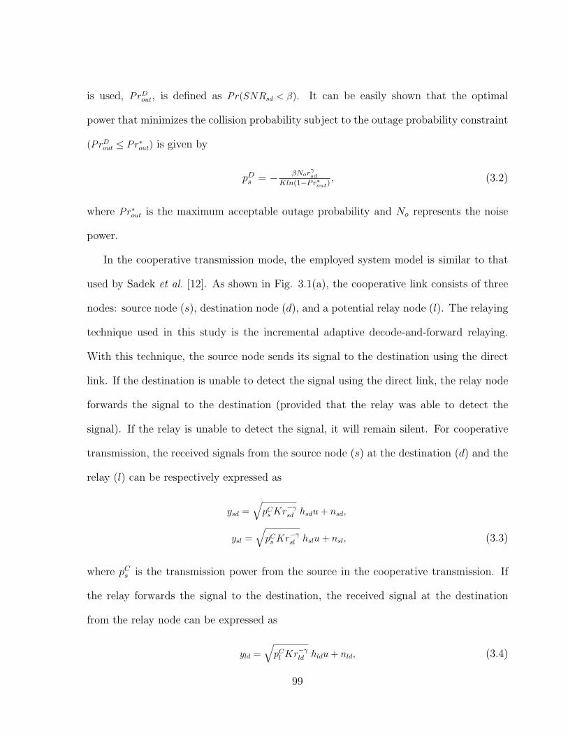
is used, PrDout, is defined as Pr(SNRsd < β). It can be easily shown that the optimal

power that minimizes the collision probability subject to the outage probability constraint

(PrDout ≤ Pr∗out) is given by

pDs = − βNorγsd

Kln(1−Pr∗out), (3.2)

where Pr∗out is the maximum acceptable outage probability and No represents the noise

power.

In the cooperative transmission mode, the employed system model is similar to that

used by Sadek et al. [12]. As shown in Fig. 3.1(a), the cooperative link consists of three

nodes: source node (s), destination node (d), and a potential relay node (l). The relaying

technique used in this study is the incremental adaptive decode-and-forward relaying.

With this technique, the source node sends its signal to the destination using the direct

link. If the destination is unable to detect the signal using the direct link, the relay node

forwards the signal to the destination (provided that the relay was able to detect the

signal). If the relay is unable to detect the signal, it will remain silent. For cooperative

transmission, the received signals from the source node (s) at the destination (d) and the

relay (l) can be respectively expressed as

ysd =√pCs Kr

−γsd hsdu+ nsd,

ysl =√pCs Kr

−γsl hslu+ nsl, (3.3)

where pCs is the transmission power from the source in the cooperative transmission. If

the relay forwards the signal to the destination, the received signal at the destination

from the relay node can be expressed as

yld =√pCl Kr

−γld hldu+ nld, (3.4)

99

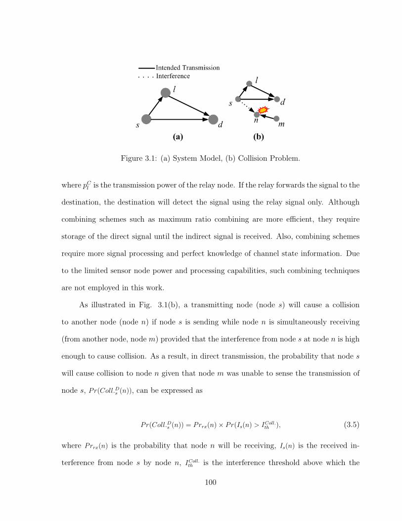
Figure 3.1: (a) System Model, (b) Collision Problem.

where pCl is the transmission power of the relay node. If the relay forwards the signal to the

destination, the destination will detect the signal using the relay signal only. Although

combining schemes such as maximum ratio combining are more efficient, they require

storage of the direct signal until the indirect signal is received. Also, combining schemes

require more signal processing and perfect knowledge of channel state information. Due

to the limited sensor node power and processing capabilities, such combining techniques

are not employed in this work.

As illustrated in Fig. 3.1(b), a transmitting node (node s) will cause a collision

to another node (node n) if node s is sending while node n is simultaneously receiving

(from another node, node m) provided that the interference from node s at node n is high

enough to cause collision. As a result, in direct transmission, the probability that node s

will cause collision to node n given that node m was unable to sense the transmission of

node s, Pr(Coll.Ds (n)), can be expressed as

Pr(Coll.Ds (n)) = Prrx(n)× Pr(Is(n) > IColl.th ), (3.5)

where Prrx(n) is the probability that node n will be receiving, Is(n) is the received in-

terference from node s by node n, IColl.th is the interference threshold above which the

100

interference causes collision and the desired signal is undetectable.

Employing the CSMA-CA mechanism for channel access, nodes that are within the

sensing range of a transmitter are inhibited from the transmission. Therefore, the prob-

ability that node s will cause a collision to one or more nodes in the network is given

by

Pr(Coll.Ds ) = 1−∏n∈N

(1− Pr

(Coll.Ds (n)

)Pr (NSTs)

), (3.6)

where N is the set of all nodes in the network except node s and d, and Pr(NSTs) is the

average probability of not sensing transmission of node s, i.e.,

Pr (NSTs) =∑m∈N

Pr(Is(m) < ISens.th )Prtx(m), (3.7)

where ISens.th is the carrier sensing threshold above which the channel is deemed busy and

Prtx(m) is the probability that node m is transmitting.

The traffic model assumed to be a Poisson arrival process. Therefore, the probability

of being receiving (or transmitting) is given by

Prrx (m)=Prtx (m)= 1

bN−22 c

∑bN−22 c

j=1 e−µmTp [µmTp]j

(j−1)!, (3.8)

where N is the number of nodes in the network, Tp denotes the packet duration, and µm

is the average transmission rate (packet/sec.) of node m.

Since incremental relaying is used, the average collision probability caused by the

cooperative link to all other nodes in the network is equal to the collision probability

caused by the source node, Pr(Coll.Ds ), if the direct signal (from the source) is detectable

at the destination, or if the relay node is unable to detect the source signal. Otherwise,

the collision probability is the union of collision probability caused by the source node,

101

and the collision probability caused by the relay node, Pr(Coll.Dl ). Thus, the collision

probability caused by the cooperative transmission (from s and l) to all other nodes in

the network is given by

Pr(Coll.Cs,l

)= (3.9)Pr

(Coll.Ds

), (SNRsd > β)or(SNRsd < β&SNRsl < β)

Pr(Coll.Ds

⋃Coll.Dl

), (SNRsd < β&SNRsl > β),

where SNRsl is the SNR of the source-relay link.

Since the fading coefficient follows the Rayleigh distribution, the SNR follows the

exponential distribution and by substituting Eq. (3.6) into Eq. (3.9) and after some

simplification, Pr(Coll.Cs,l

)can be expressed as in Eq. (3.10).

Pr(Coll.Cs,l

)=

(1−

∏n∈N

[1− Prrx (n)Pr

(Is(n) > IColl.th

)∑m∈N

Prtx (m)Pr(Is(m) < ISens.th

)])

+

(1−

∏n∈N

[1− Prrx (n)Pr

(Il(n) > IColl.th

)∑m∈N

Prtx (m)Pr(Il(m) < ISens.th

)])Pr(SNRsd < β) Pr(SNRsl > β)

−

(1−

∏n∈N

[1− Prrx (n)Pr

(Is(n) > IColl.th

)∑m∈N

Prtx (m)Pr(Is(m) < ISens.th

)])

×

(1−

∏n∈N

[1− Prrx (n)Pr

(Il(n) > IColl.th

)∑m∈N

Prtx (m)Pr (Il(m) < CSth)

])Pr(SNRsd < β) Pr(SNRsl > β), (3.10)

In general, a route is a concatenation of cooperative transmission and direct transmis-

sion links. Therefore, the collision probability caused by the entire route to all nodes in

the network can be expressed as

Pr(Coll.route) = Pr

(H⋃h=1

(Coll.Csh,lhIn

C(h) + Coll.DshInC(h)

)), (3.11)

102

where h is the hop number, H is the total number of hops in the route, and InC(h) is

the indicator function, which is equal to one if the h-th hop uses cooperative transmission

and it is equal to zero if the h-th hop uses direct transmission.

In cooperative transmission with incremental adaptive decode-and-forward, the outage

probability is given by

PrCout = Pr(SNRsd < β)Pr(SNRsl < β)+ (3.12)

Pr(SNRsd < β)Pr(SNRsl > β)Pr(SNRld < β),

where the first term of the equation refers to the event that the source-to-destination and

the source-to-relay links are in outage (i.e., SNR of each link is less than β). The second

term refers to the event that the source-to-destination and relay-to-destination links are

in outage but the source-to-relay link is not in outage.

Furthermore, the end-to-end outage probability of a certain route is defined as the

probability that outage takes place in one of the H hops of the route, i.e.,

Prout(route) = 1−H∏h=1

(1− Prout (h)) , (3.13)

where Prout (h) is the outage probability of the h-th link (either cooperative or direct) in

the route.

The goal of the algorithm is to find the route from the source to the sink that minimizes

the collision probability caused by the entire route to all nodes in the network, while

satisfying the end-to-end outage probability constraint.

103

3.4 Power Allocation in Cooperative Transmission

Links

For a given source-sink nodes, all possible routes are defined as a set of hops between the

source and destination. Thus, the problem can be formulated as a constraint optimization

problem as follows

Minps, pl

Pr(Coll.route),

s.t. Prout(route) ≤ Pr∗out. (3.14)

In a cooperative transmission link, the constrained optimization problem can be solved

using the Lagrange Multipliers method as follows

∂∂ ps

(Pr(Coll.Cs,l) + λPrCout) = 0,

∂∂ pl

(Pr(Coll.Cs,l) + λPrCout) = 0, (3.15)

PrCout = Pr∗out , λ > 0,

where λ is the Lagrange Multiplier. Using the exponential distribution of the SNR in Eq.

(3.12) and substituting Eqs. (3.10) and (3.12) in Eq. (3.15) and after some manipulations,

Eq. (3.15) can be rewritten as Eqs. (3.16), (3.17), and (3.18).

∑n∈N

[IColl.th rγsnKp2

s

φ (ps, n)− θ (ps, n)

] ∏m∈N

[1− φ (ps,m)]

[1−

(1−

∏n∈N

[1− φ (pl, n)]

)(exp

(−k2ps

)− exp

(−k1+k2

ps

))]

−

(1−

∏n∈N

[1− φ (pl, n)]

)(k1p2s

)exp

(−k1+k2

ps

)+

(1−

∏n∈N

[1− φ (pl, n)]

)

104

(exp

(−k2ps

)− exp

(−k1+k2

ps

))k2p2s

+

(1−

∏n∈N

[1− φ (ps, n)]

)(

1−∏n∈N

[1− φ (pl, n)]

)(k1+k2p2s

exp(−k1+k2

ps

)+ k2

p2sexp

(−k2ps

))−λk1

p2sexp

(−k1ps

)− λk2

p2sexp

(−(k2ps

+ k3pl

))− λ(k1+k2)

p2sexp

(−k1+k2

ps− k3

pl

)= 0, (3.16)

∑n∈N

Ithr

γsn

Kp2l

φ (pl, n)− θ (pl, n)∏m∈N

[1− φ (pl,m)]

×[exp

(−k2ps

)− exp

(−k1+k2

ps

)] ∏m∈N

[1− φ (ps,m)]

−λk3p2l

[exp

(−k2ps− k3

pl

)+exp

(−k1+k2

ps− k3

pl

)]=0, (3.17)

1−exp(−k1ps

)−exp

(−k2ps− k3

pl

)−exp(k1+k2

ps+ k3

pl)=Pr∗out, (3.18)

where k1 =Noβr

γsd

K, k2 =

Noβrγsl

K, and k3 =

Noβrγld

K. Moreover, φ (p, n) and θ (p, n) are defined as

follows

φ (p, n) = Prrx (n) exp(− IColl.th rγsn

K p

)×∑m∈N

Prtx (m)

(1− exp

(−I

Sens.th rγsmK p

)),

θ (p, n) = Prrx (n) exp(− IColl.th rγsn

K p

)×∑m∈N

Prtx (m)ISens.th rγsmK p2

exp

(−I

Sens.th rγsmK p

).

These three expressions (Eqs. 3.16 - 3.18) are solved simultaneously to determine ps

and pl.

105

3.5 Proposed Cooperative Routing for Collision Min-

imization

In this section, we propose an algorithm to minimize the collision probability that a route

causes to all nodes in the network through collision-aware route selection. This is achieved

by selecting links which cause low collision probability to other nodes in the network. In

addition, the algorithm uses cooperative transmission and power allocation jointly to re-

duce the collision probability, while the outage probability is kept below the targeted

value.

As discussed before, finding the optimal cooperative route appears to be NP-hard and

has a complexity of O(22N). Therefore, we propose the sub-optimal cooperative routing:

Minimum Collision Cooperative Routing (MCCR). This algorithm requires a polynomial

time complexity to determine the route that causes minimum collision probability in the

network. MCCR is implemented using the following steps:

Step 1 : Each node in the network calculates the collision probability caused because

of transmitting a signal from node i to node j as the minimum of Pr(Coll.D) (from Eq.

3.6) and Pr(Coll.C) (from Eq. 3.9). This probability is used as the cost function of link

i-j. The calculation is done using the initial transmission power (for the source and relay

nodes), which is assumed to be 10 dBm, which is the standard value in IEEE 802.15.4

devices [13]. Since the optimum relay location in the decode-and-forward relaying tech-

nique is almost at the middle point between s and d, in cooperative links [14], we select

a relay node (k) that is closest to the middle point of each link.

Step 2 : The Bellman-Ford algorithm is applied to find the route which has the min-

imum cost function of the entire route. Therefore, the route which causes the minimum

106

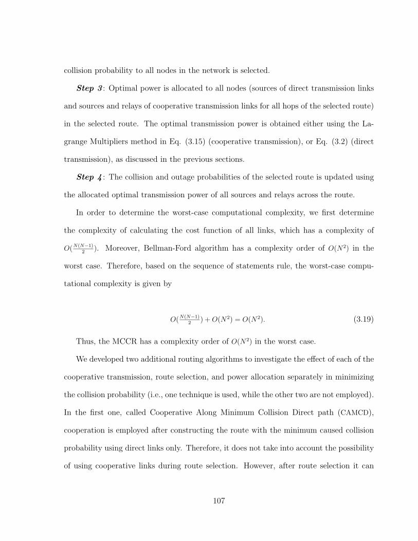
collision probability to all nodes in the network is selected.

Step 3 : Optimal power is allocated to all nodes (sources of direct transmission links

and sources and relays of cooperative transmission links for all hops of the selected route)

in the selected route. The optimal transmission power is obtained either using the La-

grange Multipliers method in Eq. (3.15) (cooperative transmission), or Eq. (3.2) (direct

transmission), as discussed in the previous sections.

Step 4 : The collision and outage probabilities of the selected route is updated using

the allocated optimal transmission power of all sources and relays across the route.

In order to determine the worst-case computational complexity, we first determine

the complexity of calculating the cost function of all links, which has a complexity of

O(N(N−1)2

). Moreover, Bellman-Ford algorithm has a complexity order of O(N2) in the

worst case. Therefore, based on the sequence of statements rule, the worst-case compu-

tational complexity is given by

O(N(N−1)2

) +O(N2) = O(N2). (3.19)

Thus, the MCCR has a complexity order of O(N2) in the worst case.

We developed two additional routing algorithms to investigate the effect of each of the

cooperative transmission, route selection, and power allocation separately in minimizing

the collision probability (i.e., one technique is used, while the other two are not employed).

In the first one, called Cooperative Along Minimum Collision Direct path (CAMCD),

cooperation is employed after constructing the route with the minimum caused collision

probability using direct links only. Therefore, it does not take into account the possibility

of using cooperative links during route selection. However, after route selection it can

107

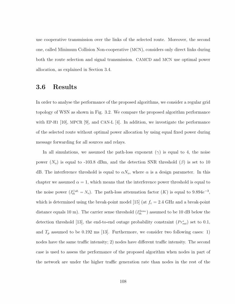
use cooperative transmission over the links of the selected route. Moreover, the second

one, called Minimum Collision Non-cooperative (MCN), considers only direct links during

both the route selection and signal transmission. CAMCD and MCN use optimal power

allocation, as explained in Section 3.4.

3.6 Results

In order to analyse the performance of the proposed algorithms, we consider a regular grid

topology of WSN as shown in Fig. 3.2. We compare the proposed algorithm performance

with EP-H1 [10], MPCR [9], and CAN-L [4]. In addition, we investigate the performance

of the selected route without optimal power allocation by using equal fixed power during

message forwarding for all sources and relays.

In all simulations, we assumed the path-loss exponent (γ) is equal to 4, the noise

power (No) is equal to -103.8 dBm, and the detection SNR threshold (β) is set to 10

dB. The interference threshold is equal to αNo, where α is a design parameter. In this

chapter we assumed α = 1, which means that the interference power threshold is equal to

the noise power (IColl.th = No). The path-loss attenuation factor (K) is equal to 9.894e−3,

which is determined using the break-point model [15] (at fc = 2.4 GHz and a break-point

distance equals 10 m). The carrier sense threshold (ISens.th ) assumed to be 10 dB below the

detection threshold [13], the end-to-end outage probability constraint (Pr∗out) set to 0.1,

and Tp assumed to be 0.192 ms [13]. Furthermore, we consider two following cases: 1)

nodes have the same traffic intensity; 2) nodes have different traffic intensity. The second

case is used to assess the performance of the proposed algorithm when nodes in part of

the network are under the higher traffic generation rate than nodes in the rest of the

108

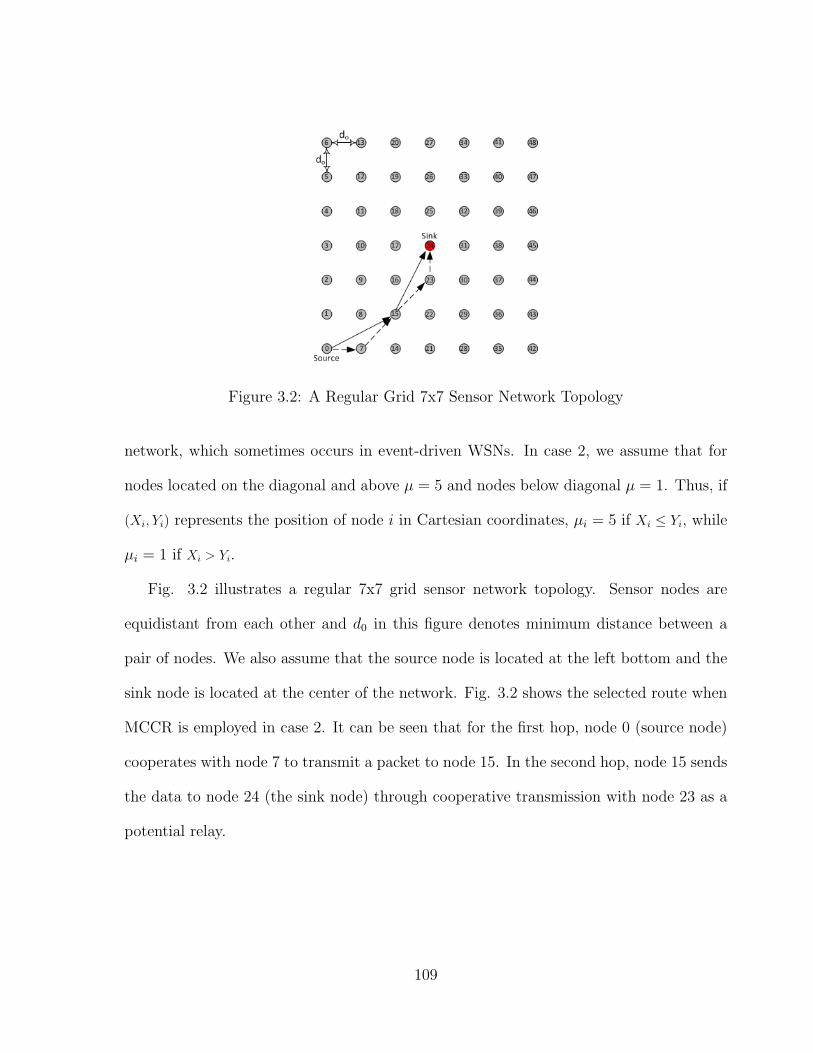
Figure 3.2: A Regular Grid 7x7 Sensor Network Topology

network, which sometimes occurs in event-driven WSNs. In case 2, we assume that for

nodes located on the diagonal and above µ = 5 and nodes below diagonal µ = 1. Thus, if

(Xi, Yi) represents the position of node i in Cartesian coordinates, µi = 5 if Xi ≤ Yi, while

µi = 1 if Xi > Yi.

Fig. 3.2 illustrates a regular 7x7 grid sensor network topology. Sensor nodes are

equidistant from each other and d0 in this figure denotes minimum distance between a

pair of nodes. We also assume that the source node is located at the left bottom and the

sink node is located at the center of the network. Fig. 3.2 shows the selected route when

MCCR is employed in case 2. It can be seen that for the first hop, node 0 (source node)

cooperates with node 7 to transmit a packet to node 15. In the second hop, node 15 sends

the data to node 24 (the sink node) through cooperative transmission with node 23 as a

potential relay.

109

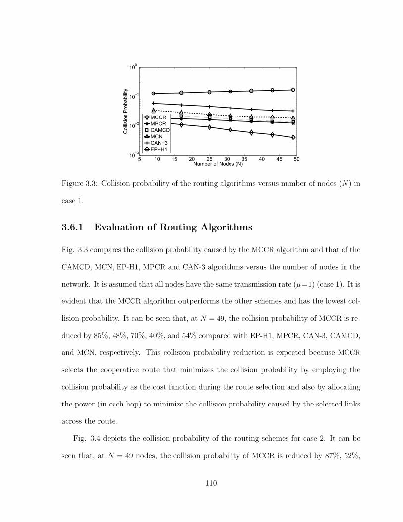
5 10 15 20 25 30 35 40 45 5010−3

10−2

10−1

100

Number of Nodes (N)

Col

lisio

n Pr

obab

ility

MCCRMPCRCAMCDMCNCAN−3EP−H1

Figure 3.3: Collision probability of the routing algorithms versus number of nodes (N) in

case 1.

3.6.1 Evaluation of Routing Algorithms

Fig. 3.3 compares the collision probability caused by the MCCR algorithm and that of the

CAMCD, MCN, EP-H1, MPCR and CAN-3 algorithms versus the number of nodes in the

network. It is assumed that all nodes have the same transmission rate (µ=1) (case 1). It is

evident that the MCCR algorithm outperforms the other schemes and has the lowest col-

lision probability. It can be seen that, at N = 49, the collision probability of MCCR is re-

duced by 85%, 48%, 70%, 40%, and 54% compared with EP-H1, MPCR, CAN-3, CAMCD,

and MCN, respectively. This collision probability reduction is expected because MCCR

selects the cooperative route that minimizes the collision probability by employing the

collision probability as the cost function during the route selection and also by allocating

the power (in each hop) to minimize the collision probability caused by the selected links

across the route.

Fig. 3.4 depicts the collision probability of the routing schemes for case 2. It can be

seen that, at N = 49 nodes, the collision probability of MCCR is reduced by 87%, 52%,

110

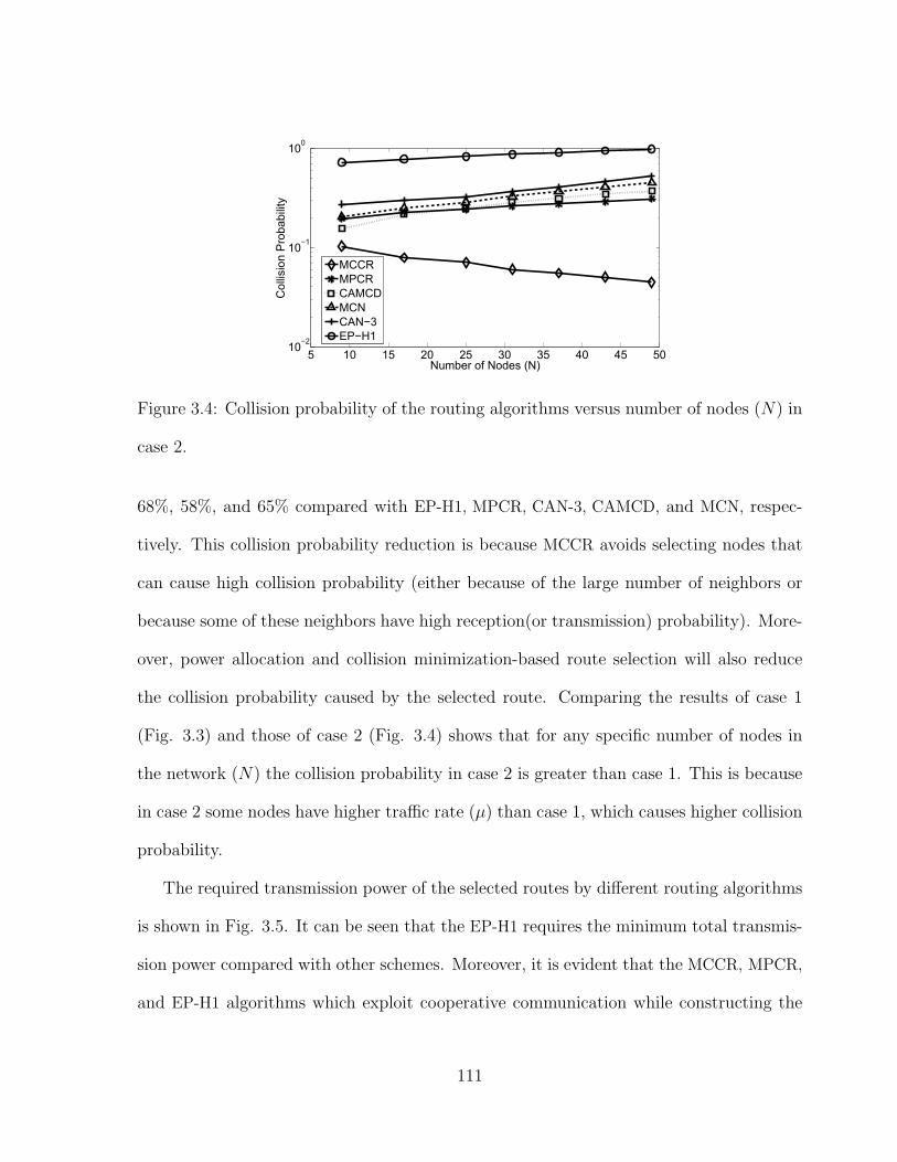
5 10 15 20 25 30 35 40 45 5010−2

10−1

100

Number of Nodes (N)

Col

lisio

n Pr

obab

ility


Figure 3.4: Collision probability of the routing algorithms versus number of nodes (N) in

case 2.

68%, 58%, and 65% compared with EP-H1, MPCR, CAN-3, CAMCD, and MCN, respec-

tively. This collision probability reduction is because MCCR avoids selecting nodes that

can cause high collision probability (either because of the large number of neighbors or

because some of these neighbors have high reception(or transmission) probability). More-

over, power allocation and collision minimization-based route selection will also reduce

the collision probability caused by the selected route. Comparing the results of case 1

(Fig. 3.3) and those of case 2 (Fig. 3.4) shows that for any specific number of nodes in

the network (N) the collision probability in case 2 is greater than case 1. This is because

in case 2 some nodes have higher traffic rate (µ) than case 1, which causes higher collision

probability.

The required transmission power of the selected routes by different routing algorithms

is shown in Fig. 3.5. It can be seen that the EP-H1 requires the minimum total transmis-

sion power compared with other schemes. Moreover, it is evident that the MCCR, MPCR,

and EP-H1 algorithms which exploit cooperative communication while constructing the

111

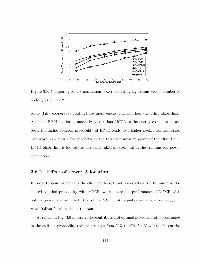
5 10 15 20 25 30 35 40 45 5010−3

10−2

10−1

100

Number of Nodes (N)

Tota

l Tra

nsm

issi

on P

ower

in d

B


Figure 3.5: Comparing total transmission power of routing algorithms versus number of

nodes (N) in case 2.

route (fully cooperative routing) are more energy efficient than the other algorithms.

Although EP-H1 performs modestly better than MCCR in the energy consumption as-

pect, the higher collision probability of EP-H1 leads to a higher packet retransmission

rate which can reduce the gap between the total transmission power of the MCCR and

EP-H1 algorithm, if the retransmission is taken into account in the transmission power

calculation.

3.6.2 Effect of Power Allocation

In order to gain insight into the effect of the optimal power allocation to minimize the

caused collision probability with MCCR, we compare the performance of MCCR with

optimal power allocation with that of the MCCR with equal power allocation (i.e., ps =

pl = 10 dBm for all nodes in the route).

As shown in Fig. 3.6 in case 2, the contribution of optimal power allocation technique

in the collision probability reduction ranges from 39% to 47% for N = 9 to 49. On the

112

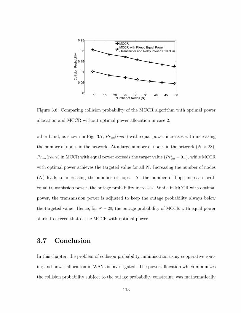
5 10 15 20 25 30 35 40 45 500

0.05

0.1

0.15

0.2

0.25

Number of Nodes (N)

Col

lisio

n Pr

obab

ility

MCCRMCCR with Fixeed Equal Power(Transmitter and Relay Power = 10 dBm

Figure 3.6: Comparing collision probability of the MCCR algorithm with optimal power

allocation and MCCR without optimal power allocation in case 2.

other hand, as shown in Fig. 3.7, Prout(route) with equal power increases with increasing

the number of nodes in the network. At a large number of nodes in the network (N > 28),

Prout(route) in MCCR with equal power exceeds the target value (Pr∗out = 0.1), while MCCR

with optimal power achieves the targeted value for all N . Increasing the number of nodes

(N) leads to increasing the number of hops. As the number of hops increases with

equal transmission power, the outage probability increases. While in MCCR with optimal

power, the transmission power is adjusted to keep the outage probability always below

the targeted value. Hence, for N = 28, the outage probability of MCCR with equal power

starts to exceed that of the MCCR with optimal power.

3.7 Conclusion

In this chapter, the problem of collision probability minimization using cooperative rout-

ing and power allocation in WSNs is investigated. The power allocation which minimizes

the collision probability subject to the outage probability constraint, was mathematically

113

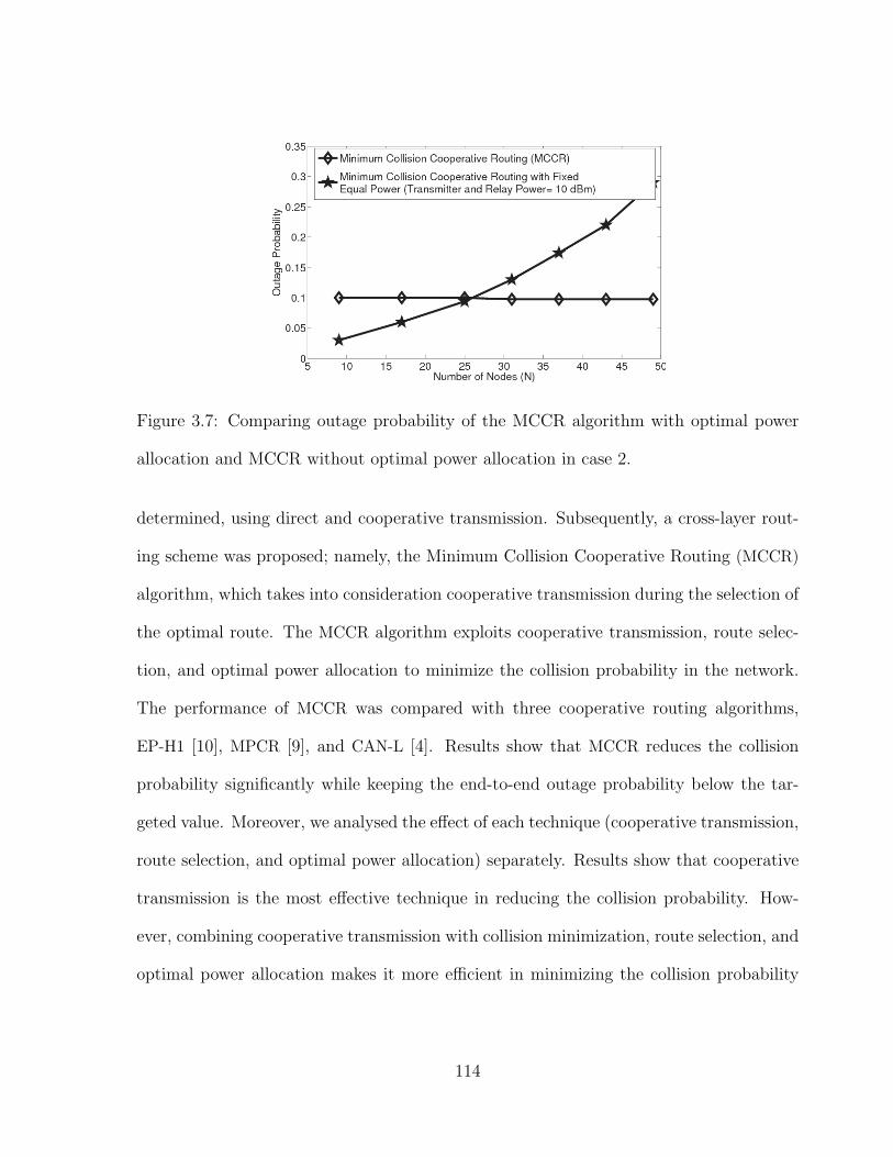
Figure 3.7: Comparing outage probability of the MCCR algorithm with optimal power

allocation and MCCR without optimal power allocation in case 2.

determined, using direct and cooperative transmission. Subsequently, a cross-layer rout-

ing scheme was proposed; namely, the Minimum Collision Cooperative Routing (MCCR)

algorithm, which takes into consideration cooperative transmission during the selection of

the optimal route. The MCCR algorithm exploits cooperative transmission, route selec-

tion, and optimal power allocation to minimize the collision probability in the network.

The performance of MCCR was compared with three cooperative routing algorithms,

EP-H1 [10], MPCR [9], and CAN-L [4]. Results show that MCCR reduces the collision

probability significantly while keeping the end-to-end outage probability below the tar-

geted value. Moreover, we analysed the effect of each technique (cooperative transmission,

route selection, and optimal power allocation) separately. Results show that cooperative

transmission is the most effective technique in reducing the collision probability. How-

ever, combining cooperative transmission with collision minimization, route selection, and

optimal power allocation makes it more efficient in minimizing the collision probability

114

with a small increase in the transmission power compared to other routing schemes.

REFERENCES



pp. 3062–3080, Dec. 2004.

[2] Z. Zhou, S. Zhou, J.-H. Cui, and S. Cui, “Energy-efficient cooperative communication

based on power control and selective single-relay in wireless sensor networks,” IEEE

Trans. Wireless Commun., vol. 7, no. 8, pp. 3066 –3078, Aug. 2008.

[3] Y.-W. Hong, W.-J. Huang, F.-H. Chiu, and C.-C. Kuo, “Cooperative communica-

tions in resource-constrained wireless networks,” IEEE Signal Process. Mag., May

2007.

[4] A. E. Khandani, J. Abounadi, E. Modiano, and L. Zheng, “Cooperative routing

in static wireless networks,” IEEE Trans. Wireless Commun., vol. 55, no. 11, pp.

2185–2192, Nov. 2007.

[5] A. Ahluwalia and E. Modiano, “On the complexity and distributed construction of

energy-efficient broadcast trees in wireless ad hoc networks,” IEEE Trans. Wireless

Commun., vol. 4, no. 5, pp. 2136 – 2147, Sep. 2005.

115

[6] Z. Yang and A. Høst-Madsen, “Routing and power allocation in asynchronous gaus-

sian multiple-relay channels,” EURASIP J. Wirel. Commun. Netw., vol. 2006, no. 2,

pp. 35–35, Apr. 2006.

[7] J. Zhang and Q. Zhang, “Cooperative routing in multi-source multi-destination

multi-hop wireless networks,” in Proc. IEEE The 27th Conference on Computer

Communications (INFOCOM’08), Apr. 2008, pp. 2369 –2377.

[8] F. Li, K. Wu, and A. Lippman, “Energy-efficient cooperative routing in multi-hop

wireless ad hoc networks,” in Proc. IEEE 25th International Performance, Comput-

ing, and Communications Conference, (IPCCC’06), Apr. 2006, pp. 214–222.


wireless networks,” IEEE Trans. Wireless Commun., vol. 7, no. 10, pp. 3930 –3941,

Oct. 2008.

[10] M. Dehghan, M. Ghaderi, and D. Goeckel, “Minimum-energy cooperative routing in

wireless networks with channel variations,” IEEE Trans. Wireless Commun., vol. 10,

no. 11, pp. 3813–3823, Nov. 2011.

[11] C. Zhai, J. Liu, L. Zheng, H. Xu, and H. Chen, “Maximise lifetime of wireless sensor

networks via a distributed cooperative routing algorithm,” Transactions on Emerging

Telecommunications Technologies, vol. 23, no. 5, pp. 414 –428, Aug. 2012.

[12] A. K. Sadek, W. Yu, and K. J. R. Liu, “On the energy efficiency of cooperative

communications in wireless sensor networks,” IEEE/ACM Trans. Netw., vol. 6, no. 1,

pp. 1–21, Jan. 2010.

116

[13] Wireless Medium Access Control (MAC) and Physical Layer (PHY) Specications for

Low-Rate Wireless Personal Area Networks (WPANs), IEEE Std. 802.15.4, 2011.

[14] B. Han, J. Li, and J. Su, “Optimal relay node placement for multi-pair cooperative

communication in wireless networks,” in Proc. IEEE Wireless Communications and

Networking Conference (WCNC), Apr. 2013, pp. 4724–4729.

[15] A. Molisch, Wireless Communications, 2nd ed. Wiley-IEEE Press, 2005.

117

Chapter 4

Per-Node Traffic Load in

Cooperative Wireless Sensor

Networks

4.1 Abstract


fading without using multiple antennas. In multi-hop wireless networks, such as wireless

sensor networks, per-node traffic load helps to provide important insights into designing

efficient network protocols. Cooperative diversity introduces new aspects to the per-node

traffic load. In this chapter, we present an analytical model for estimating the per-node

traffic load in a cooperative wireless sensor network. We consider a typical scenario,

wherein the sensor nodes sense the environment and forwards the events to a sink node

using the greedy geographical routing. Our results confirm that traffic load increases as a

118

function of the node’s vicinity to the sink node. Simulation results validate the accuracy

of our analytical model.

4.2 Introduction

Cooperative diversity has been proposed as an effective technique to improve the robust-

ness of wireless links [1]. This technique is particularly appropriate for densely populated

and randomly deployed networks, such as Wireless Sensor Networks (WSNs). Cooperative

diversity exploits neighboring sensor nodes in order to relay the packets from transmit-

ting nodes to the intended destinations. Combining multiple copies of the same signal at

the destination leads to several advantages, such as the better signal quality and higher

capacity.

In WSNs, upon the detection of an event, packet traffic load in some spots may

become intensified, resulting in a high packet collision rate and consequently, packet loss.

Moreover, it has been well accepted that the sensor nodes close to the sink node (base

station) become heavily involved in packet forwarding and thus, they carry high traffic

load. As a result, the sensor nodes close to the sink quickly drain batteries, leading to

a possible network disconnection and the functional network lifetime reduction. Similar

to other multi-hop networks, in WSNs each node relays the traffic of other nodes in the

network. Hence, the traffic load of each node includes the traffic generated by the node,

as well as the traffic generated by other nodes, which is relayed by this node. Thus, the

per-node traffic load can be defined as the average number of packets transmitted by the

sensor node during a time unit [2]. The analytical calculation of the per-node traffic load

helps in designing and configuring efficient network protocols. For instance, an analytical

119

model to accurately estimate the traffic load of each node can be used to maximize the

network lifetime by balancing the sensor node traffic load [3] or to minimize the packet

collision probability [4].

Cooperative diversity introduces new aspects to the typical traffic load of the nodes

in WSNs. A relay node in a cooperative link not only receives traffic load from the

transmitter node, but also forwards the traffic load to the destination node. To the best

of our knowledge, there is no analytical model which can accurately characterize the per-

node traffic load in a cooperative wireless network. The available model for estimating

the per-node traffic load, presented in [2], does not incorporate cooperative diversity and

its implication in the network. This Chapter presents a new and detailed analytical model

for calculating the per-node traffic load in cooperative WSNs.

The rest of this chapter is organized as follows. In Section 4.3, we provide an overview

of the system model. In Section 4.4, the analysis of the per-node traffic load is presented.

Section 4.5 validates the analytical model by comparing the analytical results with those

obtained by simulations. Finally, Section 4.6 concludes the Chapter.

4.3 System Model

We focus on event driven applications, wherein the source nodes forward the event (e.g.

fire, target detection) to the sink node. A large portion of WSNs deployed today falls

into this category (e.g., RIMBAMON [5]). With regards to the routing strategy, we have

considered the popular greedy routing forwarding scheme [6]. In greedy routing, a sensor

node forwards its packets to a neighbor, which is the closest geographically to the sink

node amongst possible neighboring nodes. As a result, greedy routing can approximately

120

find the shortest path in terms of hops between a sensor node and the sink node. Moreover,

greedy routing is a scalable routing solution for large WSNs, because it only requires local

(i.e., one hop neighborhood) information for making a forwarding decision. However, the

proposed model is not limited to the greedy routing and other types of routing algorithms

can also be considered in the analysis. Similar to [2], we assume that the sensor nodes

are uniformly randomly deployed in a circular disc, while the sink node is located at the

center. Upon detecting an event, the source nodes generate a data packet, containing the

relevant sensed data, and routes the packet toward the sink node. The packet generation

follows the Poisson model with a rate of λ packets per second.

The wireless channel is assumed to suffer from Rayleigh fading. Variables |hij| and nij

represent the Rayleigh fading channel coefficient and the additive white Gaussian noise

of the link between nodes i and j, respectively. We also assume that the distance-based

attenuation follows the generic exponential path-loss model with an exponent γ [7, 8].

For the cooperative system model, similar to [7], we use incremental relaying with

adaptive decode-and-forward relaying. As such, the source node sends its signal to the

destination using the direct link. If the destination is not able to detect the signal using

the direct signal, the destination sends a negative acknowledgement (NACK) signal to

the relay. Consequently, the relay node forwards the signal to the destination (provided

that the relay was able to detect the signal). Since the optimum relay location in the

decode-and-forward relaying technique is at the middle point between the transmitter and

the receiver nodes of a cooperative link [9], we select the closest node to the middle point

of each link as the relay node.

Although diversity combining schemes such as maximum ratio combining, are more ef-

ficient than selection combining, they require storage of the direct signal until the indirect

121

signal is received. Moreover, more signal processing and perfect knowledge of the channel

state information are required for combining schemes. Due to the limited resources at

sensor nodes, such combining techniques are not employed.

In direct transmission, where a source node (s) transmits its signal directly to the

destination node (d), the received signal at d is given by ysd =√pDs Kr

−γsd hsdu + nsd,


is a constant that depends on the characteristics of the transmitter, the receiver, and

channel (e.g., the frequency and the antenna gain), rsd is the distance between the two

nodes (s and d), and u is the transmitted data with a unity power.

In the cooperative transmission mode, the employed system model is similar to that

used by Sadek et al. [7]. The cooperative link consists of three nodes: a source node, s,

a destination node, d, and a potential relay node, l. Recall that the relaying technique

used in this study is the incremental adaptive decode-and-forward relaying. With this

technique, node s sends its signal to node d using a direct link. If d is unable to detect the

signal using the direct link, node l forwards the signal to d (provided that l was able to

detect the signal). If l is unable to detect the signal, it will remain silent. For cooperative

transmission, the received signals from the source node (s) at the destination (d) and the

relay (l) can be respectively expressed as

ysd =√pCs Kr

−γsd hsdu+ nsd,

ysl =√pCs Kr


where pCs is the transmission power from the source in the cooperative scenario. If the

relay forwards the signal to the destination, the received signal at the destination from

122

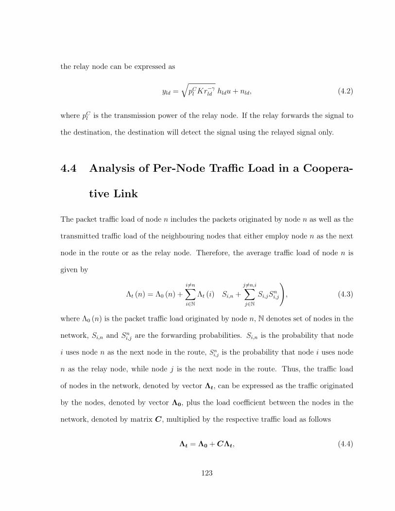
the relay node can be expressed as

yld =

√pCl Kr

−γld hldu+ nld, (4.2)

where pCl is the transmission power of the relay node. If the relay forwards the signal to

the destination, the destination will detect the signal using the relayed signal only.

4.4 Analysis of Per-Node Traffic Load in a Coopera-

tive Link

The packet traffic load of node n includes the packets originated by node n as well as the

transmitted traffic load of the neighbouring nodes that either employ node n as the next

node in the route or as the relay node. Therefore, the average traffic load of node n is

given by

Λt (n) = Λ0 (n) +

i6=n∑i∈N

Λt (i)

(Si,n +

j 6=n,i∑j∈N

Si,jSni,j

), (4.3)

where Λ0 (n) is the packet traffic load originated by node n, N denotes set of nodes in the

network, Si,n and Sni,j are the forwarding probabilities. Si,n is the probability that node

i uses node n as the next node in the route, Sni,j is the probability that node i uses node

n as the relay node, while node j is the next node in the route. Thus, the traffic load

of nodes in the network, denoted by vector Λt, can be expressed as the traffic originated

by the nodes, denoted by vector Λ0, plus the load coefficient between the nodes in the

network, denoted by matrix C, multiplied by the respective traffic load as follows

Λt = Λ0 + CΛt, (4.4)

123

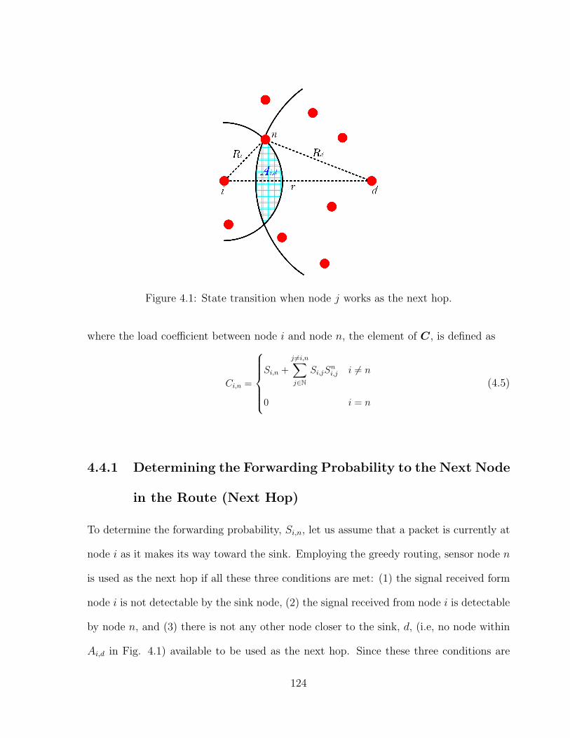
Figure 4.1: State transition when node j works as the next hop.

where the load coefficient between node i and node n, the element of C, is defined as

Ci,n =

Si,n +

j 6=i,n∑j∈N

Si,jSni,j i 6= n

0 i = n

(4.5)

4.4.1 Determining the Forwarding Probability to the Next Node

in the Route (Next Hop)

To determine the forwarding probability, Si,n, let us assume that a packet is currently at

node i as it makes its way toward the sink. Employing the greedy routing, sensor node n

is used as the next hop if all these three conditions are met: (1) the signal received form

node i is not detectable by the sink node, (2) the signal received from node i is detectable

by node n, and (3) there is not any other node closer to the sink, d, (i.e, no node within

Ai,d in Fig. 4.1) available to be used as the next hop. Since these three conditions are

124

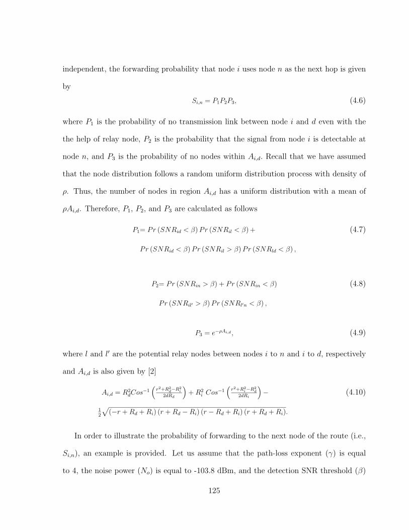
independent, the forwarding probability that node i uses node n as the next hop is given

by

Si,n = P1P2P3, (4.6)

where P1 is the probability of no transmission link between node i and d even with the

the help of relay node, P2 is the probability that the signal from node i is detectable at

node n, and P3 is the probability of no nodes within Ai,d. Recall that we have assumed

that the node distribution follows a random uniform distribution process with density of

ρ. Thus, the number of nodes in region Ai,d has a uniform distribution with a mean of

ρAi,d. Therefore, P1, P2, and P3 are calculated as follows

P1= Pr (SNRid < β)Pr (SNRil < β) + (4.7)

Pr (SNRid < β)Pr (SNRil > β)Pr (SNRld < β) ,

P2= Pr (SNRin > β) + Pr (SNRin < β) (4.8)

Pr (SNRil′ > β)Pr (SNRl′n < β) ,

P3 = e−ρAi,d , (4.9)

where l and l′ are the potential relay nodes between nodes i to n and i to d, respectively

and Ai,d is also given by [2]

Ai,d = R2dCos

−1(r2+R2

d−R2i

2dRd

)+R2

i Cos−1(r2+R2

i−R2d

2dRi

)− (4.10)

12

√(−r +Rd +Ri) (r +Rd −Ri) (r −Rd +Ri) (r +Rd +Ri).

In order to illustrate the probability of forwarding to the next node of the route (i.e.,

Si,n), an example is provided. Let us assume that the path-loss exponent (γ) is equal

to 4, the noise power (No) is equal to -103.8 dBm, and the detection SNR threshold (β)

125

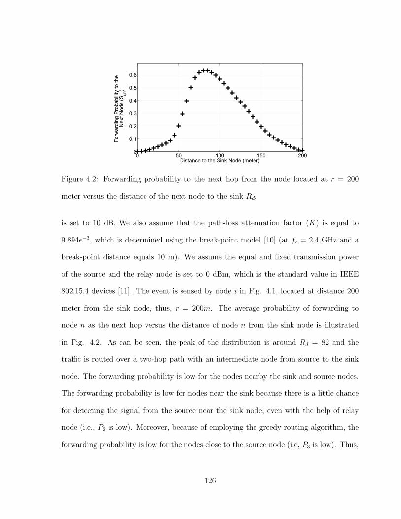
0 50 100 150 2000

0.1

0.2

0.3

0.4

0.5

0.6

Distance to the Sink Node (meter)

Forw

ardi

ng P

roba

bilit

y to

the

Nex

t Nod

e (S

i,n)

Figure 4.2: Forwarding probability to the next hop from the node located at r = 200

meter versus the distance of the next node to the sink Rd.

is set to 10 dB. We also assume that the path-loss attenuation factor (K) is equal to

9.894e−3, which is determined using the break-point model [10] (at fc = 2.4 GHz and a

break-point distance equals 10 m). We assume the equal and fixed transmission power

of the source and the relay node is set to 0 dBm, which is the standard value in IEEE

802.15.4 devices [11]. The event is sensed by node i in Fig. 4.1, located at distance 200

meter from the sink node, thus, r = 200m. The average probability of forwarding to

node n as the next hop versus the distance of node n from the sink node is illustrated

in Fig. 4.2. As can be seen, the peak of the distribution is around Rd = 82 and the

traffic is routed over a two-hop path with an intermediate node from source to the sink

node. The forwarding probability is low for the nodes nearby the sink and source nodes.

The forwarding probability is low for nodes near the sink because there is a little chance

for detecting the signal from the source near the sink node, even with the help of relay

node (i.e., P2 is low). Moreover, because of employing the greedy routing algorithm, the

forwarding probability is low for the nodes close to the source node (i.e, P3 is low). Thus,

126

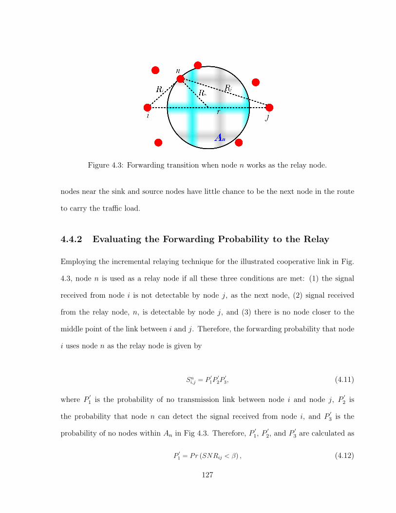
Figure 4.3: Forwarding transition when node n works as the relay node.

nodes near the sink and source nodes have little chance to be the next node in the route

to carry the traffic load.

4.4.2 Evaluating the Forwarding Probability to the Relay

Employing the incremental relaying technique for the illustrated cooperative link in Fig.

4.3, node n is used as a relay node if all these three conditions are met: (1) the signal

received from node i is not detectable by node j, as the next node, (2) signal received

from the relay node, n, is detectable by node j, and (3) there is no node closer to the

middle point of the link between i and j. Therefore, the forwarding probability that node

i uses node n as the relay node is given by

Sni,j = P′1P′2P′3, (4.11)

where P′1 is the probability of no transmission link between node i and node j, P

′2 is

the probability that node n can detect the signal received from node i, and P′3 is the

probability of no nodes within An in Fig 4.3. Therefore, P′1, P

′2, and P

′3 are calculated as

P′1 = Pr (SNRij < β) , (4.12)

127

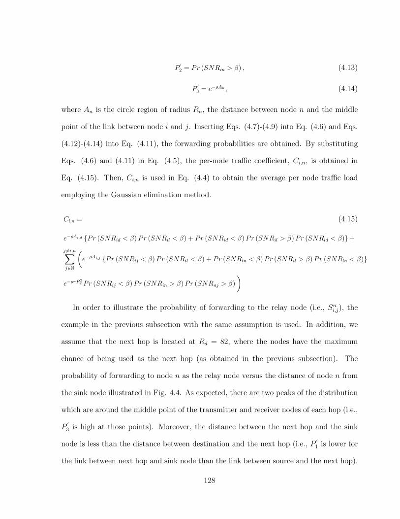
P′2 = Pr (SNRin > β) , (4.13)

P′3 = e−ρAn , (4.14)

where An is the circle region of radius Rn, the distance between node n and the middle

point of the link between node i and j. Inserting Eqs. (4.7)-(4.9) into Eq. (4.6) and Eqs.

(4.12)-(4.14) into Eq. (4.11), the forwarding probabilities are obtained. By substituting

Eqs. (4.6) and (4.11) in Eq. (4.5), the per-node traffic coefficient, Ci,n, is obtained in

Eq. (4.15). Then, Ci,n is used in Eq. (4.4) to obtain the average per node traffic load

employing the Gaussian elimination method.

Ci,n = (4.15)

e−ρAi,d Pr (SNRid < β)Pr (SNRil < β) + Pr (SNRid < β)Pr (SNRil > β)Pr (SNRld < β)+

j 6=i,n∑j∈N

(e−ρAi,j Pr (SNRij < β)Pr (SNRil < β) + Pr (SNRin < β)Pr (SNRil > β)Pr (SNRln < β)

e−ρπR2nPr (SNRij < β)Pr (SNRin > β)Pr (SNRnj > β)

)

In order to illustrate the probability of forwarding to the relay node (i.e., Sni,j), the

example in the previous subsection with the same assumption is used. In addition, we

assume that the next hop is located at Rd = 82, where the nodes have the maximum

chance of being used as the next hop (as obtained in the previous subsection). The

probability of forwarding to node n as the relay node versus the distance of node n from

the sink node illustrated in Fig. 4.4. As expected, there are two peaks of the distribution

which are around the middle point of the transmitter and receiver nodes of each hop (i.e.,

P′3 is high at those points). Moreover, the distance between the next hop and the sink

node is less than the distance between destination and the next hop (i.e., P′1 is lower for

the link between next hop and sink node than the link between source and the next hop).

128

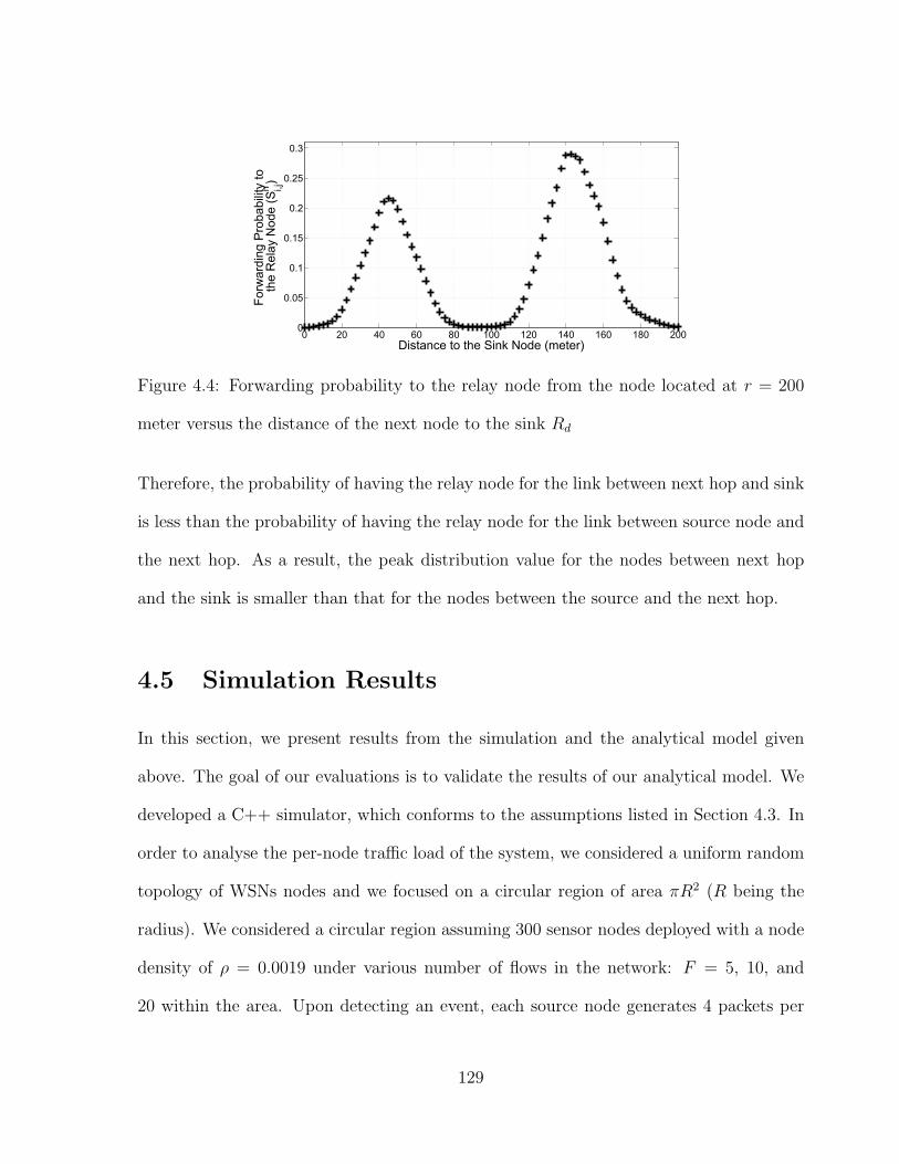
0 20 40 60 80 100 120 140 160 180 2000

0.05

0.1

0.15

0.2

0.25

0.3


Forw

ardi

ng P

roba

bilit

y to

th

e R

elay

Nod

e (S

i,jn)

Figure 4.4: Forwarding probability to the relay node from the node located at r = 200

meter versus the distance of the next node to the sink Rd

Therefore, the probability of having the relay node for the link between next hop and sink

is less than the probability of having the relay node for the link between source node and

the next hop. As a result, the peak distribution value for the nodes between next hop

and the sink is smaller than that for the nodes between the source and the next hop.

4.5 Simulation Results

In this section, we present results from the simulation and the analytical model given

above. The goal of our evaluations is to validate the results of our analytical model. We

developed a C++ simulator, which conforms to the assumptions listed in Section 4.3. In

order to analyse the per-node traffic load of the system, we considered a uniform random

topology of WSNs nodes and we focused on a circular region of area πR2 (R being the

radius). We considered a circular region assuming 300 sensor nodes deployed with a node

density of ρ = 0.0019 under various number of flows in the network: F = 5, 10, and

20 within the area. Upon detecting an event, each source node generates 4 packets per

129

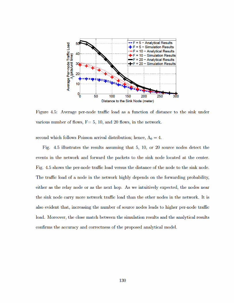
0 50 100 150 200 250 3000

10

20

30

40

50


Average Per−node Traffic Load

Λt(pkts/unit time)

F = 5 − Analytical ResultsF = 5 − Simulation ResultsF = 10 − Analytical ResultsF = 10 − Simulation ResultsF = 20 − Analytical ResultsF = 20 − Simulation Results

Figure4.5: Averageper-nodetrafficloadasafunctionofdistancetothesinkunder

variousnumberofflows,F=5,10,and20flows,inthenetwork.

secondwhichfollowsPoissonarrivaldistribution;hence,Λ0=4.

Fig.4.5illustratestheresultsassumingthat5,10,or20sourcenodesdetectthe

eventsinthenetworkandforwardthepacketstothesinknodelocatedatthecenter.

Fig.4.5showstheper-nodetrafficloadversusthedistanceofthenodetothesinknode.

Thetrafficloadofanodeinthenetworkhighlydependsontheforwardingprobability,

eitherastherelaynodeorasthenexthop.Asweintuitivelyexpected,thenodesnear

thesinknodecarrymorenetworktrafficloadthantheothernodesinthenetwork.Itis

alsoevidentthat,increasingthenumberofsourcenodesleadstohigherper-nodetraffic

load. Moreover,theclosematchbetweenthesimulationresultsandtheanalyticalresults

confirmstheaccuracyandcorrectnessoftheproposedanalyticalmodel.

130

4.6 Conclusion

In this Chapter, we proposed an accurate mathematical model to analyze the per-node

traffic load in a cooperative link. The per-node traffic load is obtained from the probability

of forwarding either as the relay or as the next hop while the packet makes its way toward

the sink. The accuracy of the analytical model is verified as there is a good match between

the analytical results and the simulation results. The simulation results reveal that the

nodes that are closer to the sink node typically have higher traffic loads. The proposed

traffic model can be extended toward several directions, such as conducting energy efficient

cooperative sensor network, or collision minimization protocols in cooperative wireless

networks. Moreover, analysis of the per-node traffic load employing other types of routing

protocols is an interesting issue for future investigation.

REFERENCES



pp. 3062–3080, Dec. 2004.

[2] Q. Chen, S. Kanhere, and M. Hassan, “Analysis of per-node traffic load in multi-

hop wireless sensor networks,” IEEE Trans. Wireless Commun., vol. 8, no. 2, pp.

958–967, Feb 2009.

131

[3] F. Bouabdallah, N. Bouabdallah, and R. Boutaba, “Load-balanced routing scheme

for energy-efficient wireless sensor networks,” in IEEE GLOBECOM0’8, Nov. 2008,

pp. 1–6.

[4] F. Mansourkiaie and M. H. Ahmed, “Joint cooperative routing and power allocation

for collision minimization in wireless sensor networks with multiple,” IEEE Commun.

Lett., vol. PP, no. 99, pp. 1–1, Sep. 2014.

[5] A. Awang and M. Suhaimi, “Rimbamon: A forest monitoring system using wireless

sensor networks,” in Proc. ICIAS, Nov 2007, pp. 1101–1106.

[6] B. Karp and H. T. Kung, “GPSR: Greedy perimeter stateless routing for wireless

networks,” in Proc. of the 6th Annual International Conference on Mobile Computing

and Networking. New York, NY, USA: ACM, Aug. 2000, pp. 243–254.

[7] A. K. Sadek, W. Yu, and K. J. R. Liu, “On the energy efficiency of cooperative

communications in wireless sensor networks,” ACM Trans. Sen. Netw., vol. 6, no. 1,

pp. 5:1–5:21, Jan. 2010.



Oct. 2008.


communication in wireless networks,” in Proc. IEEE WCNC, Apr. 2013, pp. 4724–

4729.

[10] A. Molisch, Wireless Communications, 2nd ed. Wiley-IEEE Press, 2005.

132



133

Chapter 5

Joint Cooperative Routing and

Power Allocation for Collision

Minimization in Wireless Sensor

Networks with Multiple Flows

5.1 Abstract

In this Chapter, a cross-layer cooperative routing algorithm is proposed for minimizing

the collision probability subject to an end-to-end outage probability constraint. We de-

velop a collision minimization algorithm by combining cooperative transmission, optimal

power allocation, and route selection. The proposed cooperative routing algorithm, called

Minimum Collision Cooperative Routing (MCCR), selects the route that causes mini-

mum collision probability to other nodes in the network. Results show that MCCR can

134

significantly reduce the collision probability compared with existing cooperative routing

schemes.

5.2 Introduction

Recently, cooperative diversity has been proposed as an effective technique to improve the

robustness of wireless links [1]. Cooperative diversity exploits neighboring nodes in order

to relay the packets from transmitting nodes to the intended destinations. Combining

multiple copies of the same packet at the destination leads to several advantages, such as

better signal quality and higher capacity.

Routing algorithms that take into consideration the availability of cooperative trans-

mission at the physical layer are known in the literature as cooperative routing algo-

rithms. Cooperative routing was introduced by Khandani et al. [2] and the authors also

showed that the problem of finding the optimum cooperative route is NP-hard. Therefore,

heuristic routing algorithms with reduced complexity are proposed by researchers to find

sub-optimal routes, e.g., [2, 3].

Existing cooperative routing algorithms in the literature can be divided into two cate-

gories: (1) routing algorithms which are implemented by first selecting the optimal route

based on direct transmission in each link and then using cooperative transmission over

the links of the selected route (e.g., [2]), and (2) routing algorithms which take into ac-

count the availability of the cooperative transmission on each link during route selection

(e.g., [3]). Routing schemes in the second category are more complex but more efficient.

One of the heuristic cooperative routing algorithms presented in [2] is called the Coop-

erative Along Non-cooperative (CAN-L) shortest path algorithm with the objective of

135

minimizing total transmitted power. The basic idea is to run a non-cooperative short-

est path first, and then to use cooperative transmission by the last L nodes along the

non-cooperative path. Authors in [3] presented an algorithm called Minimum Power Co-

operative Routing (MPCR). The MPCR algorithm makes routing decisions by assuming

the cooperative transmission is also available for each link. MPCR finds the route that

minimizes the total transmission power.

Interactions among multiple neighboring flows may lead to the hidden and exposed

node problems, which causes packet collision [4]. In general, cooperative routing can

improve the performance due to the more robust links and less power consumption. How-

ever, cooperative routing causes extra packet transmission by the relays. Therefore, the

gain of a cooperative routing algorithm with multiple flows is different from the one with

a single flow, especially in terms of the packet collision probability. There are only a

few papers, such as [5, 6], that considered multiple flows in cooperative routing. In [5]

collision is avoided using a contention graph approach, where a set of transmitting nodes

coordinate their transmissions to a set of receiving nodes. The algorithm approaches the

non-cooperative protocol when network congestion emerges. Moreover, in [6] the con-

gestion problem is solved in the MAC layer. The main objective of cooperative routing

in all proposed schemes is to minimize the energy consumption. However, packet col-

lision minimization, using cooperative routing, has not been addressed in the existing

schemes. Moreover, as it will be shown in the results, cooperative routing protocols, that

aim to minimize the transmitted power (e.g., MPCR and CAN-L), do not necessarily lead

to collision probability minimization. In energy constraint networks, such as Wireless

Sensor Networks (WSNs), packet collision can cause serious problems. For instance, for

target detection in security or military applications of WSNs, packet collision can lead to

136

missing the target or to long delays, which may have severe consequences. Hence, it is

desirable to minimize the collision probability in WSNs. In this chapter, we aim to design

a cross-layer cooperative routing scheme for minimizing the collision probability subject

to an end-to-end outage probability constraint. The cross-layer scheme is designed by

combining cooperative transmission, power allocation, and route selection when there are

multiple flows in the network. To the best of authors’ knowledge, this work is the first to

employ the cooperative routing for minimizing collision probability in the presence of mul-

tiple flows. We compare the proposed algorithm performance with existing cooperative

routing schemes that minimize the transmission power, such as CAN-L [2] and MPCR [3].

5.3 System Model and Problem Formulation

Let hij and nij represent the Rayleigh fading channel coefficient and the additive white

Gaussian noise of the link between nodes i and j, respectively. We assume that the

distance-based attenuation follows the generic exponential path-loss model with an expo-

nent γ [3].

In direct transmission, where a source (s) transmits its signal directly to the next

destination (d), the received signal at d is given by ysd =√pDs Kr

−γsd hsdu+ nsd, where pDs is

the transmission power from the source in the direct transmission mode, K is a constant

that depends on the characteristics of the transmitter, the receiver, and channel (e.g., the

frequency and the antenna gain), rsd is the distance between the two nodes (s and d), and

u is the transmitted data with a unity power.

The criterion for good detection is that the received signal-to-noise-ratio (SNR) must

be greater than the detection threshold (β). Outage is defined as the status when the

137

receiver is unable to detect data u. Hence, a link is considered to be in outage if the re-

ceived SNR falls below β. Thus, the outage probability, when direct transmission is only

used, PrDout, is defined as Pr(SNRsd < β). It can be easily shown that the power that mini-

mizes the collision probability subject to the outage probability constraint (PrDout ≤ Pr∗out)

is given by

pDs = − βNorγsd

K ln(1−Pr∗out), (5.1)


power.

In cooperative transmission, the employed system model is similar to that used in [3].

A cooperative link consists of three nodes: source (s), destination (d), and a potential

relay node (l). The relaying technique used in this study is the incremental adaptive

decode-and-forward. With this technique, the source sends its signal to destination using

the direct link. If the destination is unable to detect the signal using the direct link, the

relay forwards the signal to the destination (provided that the relay was able to detect the

signal). If the relay is unable to detect the signal, it will remain silent and the destination

will rely on the direct signal only. For cooperative transmission, the received signals from s

at d and l can be respectively expressed as ysd =√pCs Kr

−γsd hsdu+ nsd, ysl =

√pCs Kr

−γsl hslu+ nsl,


the relay forwards the signal to the destination, the received signal at the destination from

the relay node can be expressed as yld =√pCl Kr

−γld hldu+ nld, where pCl is the transmission

power of the relay node. In this case, the destination detects the signal using the relay

signal only. Although combining schemes such as Maximum Ratio Combining are more

efficient, they require storage of the direct signal until the indirect signal is received. Also,

138

combining schemes require more signal processing and perfect knowledge of the channel

state information. Due to the limited power and processing capabilities in WSNs, such

combining techniques are not employed in this work.

A source node, s, will cause a collision to another node, n, if s is sending while n is

simultaneously receiving (from another node, m), provided that the interference from s at

n is high enough to cause a collision. As a result, in direct transmission, the probability

that s will cause collision at n, given that m was unable to sense the transmission of s,

Pr(Coll.Ds (n)), can be expressed as

Pr(Coll.Ds (n)

)= Prrx(n)Pr(Is(n) > IColl.th ), (5.2)

where Pr(Is(n) > IColl.th ) is the probability that the received interference from s by n,

Is(n), is greater than the interference threshold, IColl.th , above which the interference causes

a collision and the desired signal is undetectable and Prrx(n) is the probability that n

will be receiving given by

Prrx(n) =

i6=n∑i∈N

Prtx (i)Ei,n +

j 6=n∑j∈N

u6=n,u6=j∑u∈N

Prtx (j)F nj,u, (5.3)

where Ei,n is a binary variable to specify whether the link between i to n is in the routing

solution, F nj,u is another binary variable to specify whether n is used as a relay node for

the link between j to u in the routing solution, and Prtx(n) is the probability that n is

transmitting, hence, Prtx(n) = Λt (n)Tp, where Tp is the packet time duration and Λt (n)

is defined as the total packet transmission rate of node n. Therefore, Λt (n) is the sum of

the packet generation rate of node itself, Λ0(n), and the transmission rate of packets that

139

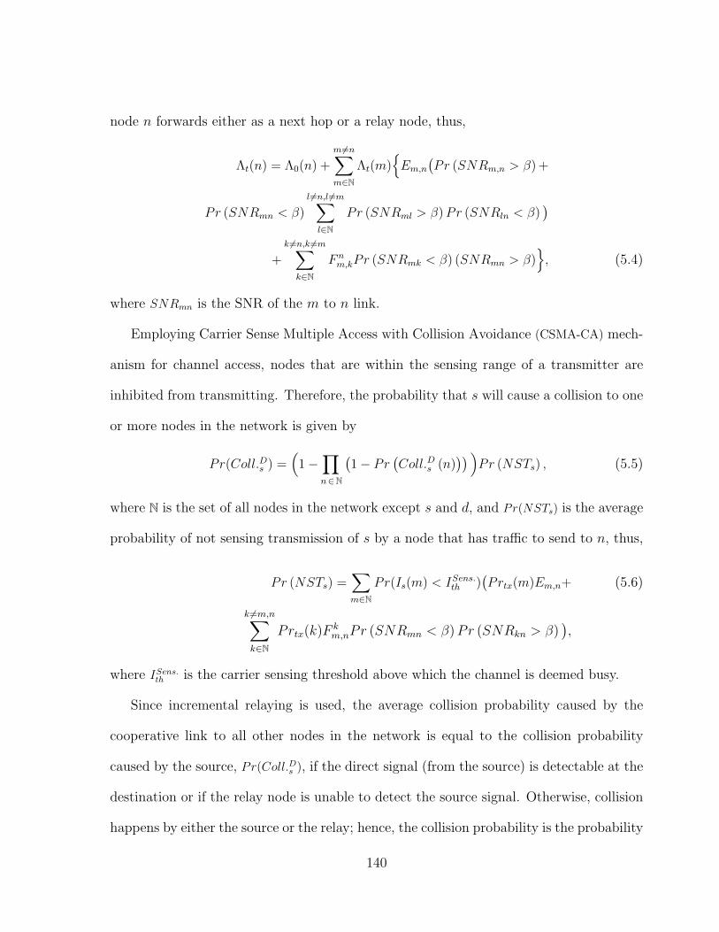
node n forwards either as a next hop or a relay node, thus,

Λt(n) = Λ0(n) +

m6=n∑m∈N

Λt(m)Em,n

(Pr (SNRm,n > β) +

Pr (SNRmn < β)

l 6=n,l 6=m∑l∈N

Pr (SNRml > β)Pr (SNRln < β))

+

k 6=n,k 6=m∑k∈N

F nm,kPr (SNRmk < β) (SNRmn > β)

, (5.4)

where SNRmn is the SNR of the m to n link.

Employing Carrier Sense Multiple Access with Collision Avoidance (CSMA-CA) mech-

anism for channel access, nodes that are within the sensing range of a transmitter are

inhibited from transmitting. Therefore, the probability that s will cause a collision to one

or more nodes in the network is given by

Pr(Coll.Ds ) =(

1−∏n∈N

(1− Pr

(Coll.Ds (n)

)) )Pr (NSTs) , (5.5)

where N is the set of all nodes in the network except s and d, and Pr(NSTs) is the average

probability of not sensing transmission of s by a node that has traffic to send to n, thus,

Pr (NSTs) =∑m∈N

Pr(Is(m) < ISens.th )(Prtx(m)Em,n+ (5.6)

k 6=m,n∑k∈N

Prtx(k)F km,nPr (SNRmn < β)Pr (SNRkn > β)

),

where ISens.th is the carrier sensing threshold above which the channel is deemed busy.



caused by the source, Pr(Coll.Ds ), if the direct signal (from the source) is detectable at the

destination or if the relay node is unable to detect the source signal. Otherwise, collision

happens by either the source or the relay; hence, the collision probability is the probability

140

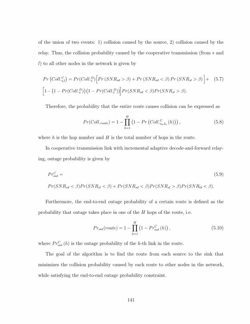
of the union of two events: 1) collision caused by the source, 2) collision caused by the

relay. Thus, the collision probability caused by the cooperative transmission (from s and

l) to all other nodes in the network is given by

Pr(Coll.Cs,l

)= Pr(Coll.Ds )

[Pr (SNRsd > β) + Pr (SNRsd < β)Pr (SNRsl > β)

]+ (5.7)[

1−(1− Pr(Coll.Ds )

)(1− Pr(Coll.Dl )

)]Pr(SNRsd < β)Pr(SNRsl > β).

Therefore, the probability that the entire route causes collision can be expressed as

Pr(Coll.route) = 1−H∏h=1

(1− Pr

(Coll.Csh,lh (h)

)), (5.8)

where h is the hop number and H is the total number of hops in the route.

In cooperative transmission link with incremental adaptive decode-and-forward relay-

ing, outage probability is given by

PrCout = (5.9)

Pr(SNRsd < β)Pr(SNRsl < β) + Pr(SNRsd < β)Pr(SNRsl > β)Pr(SNRld < β).

Furthermore, the end-to-end outage probability of a certain route is defined as the

probability that outage takes place in one of the H hops of the route, i.e.


(1− PrCout (h)

), (5.10)

where PrCout (h) is the outage probability of the h-th link in the route.

The goal of the algorithm is to find the route from each source to the sink that

minimizes the collision probability caused by each route to other nodes in the network,

while satisfying the end-to-end outage probability constraint.

141

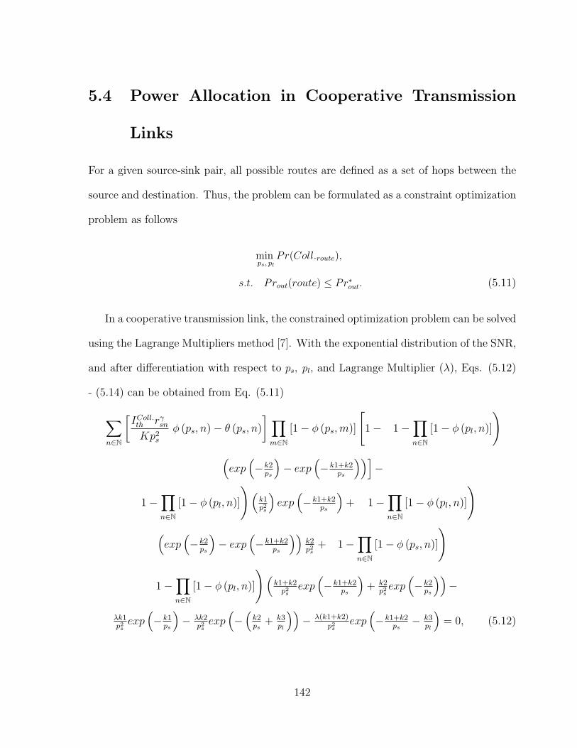
5.4 Power Allocation in Cooperative Transmission

Links

For a given source-sink pair, all possible routes are defined as a set of hops between the

source and destination. Thus, the problem can be formulated as a constraint optimization

problem as follows

minps, pl

Pr(Coll.route),

s.t. Prout(route) ≤ Pr∗out. (5.11)


using the Lagrange Multipliers method [7]. With the exponential distribution of the SNR,

and after differentiation with respect to ps, pl, and Lagrange Multiplier (λ), Eqs. (5.12)

- (5.14) can be obtained from Eq. (5.11)

∑n∈N

[IColl.th rγsnKp2

s


] ∏m∈N

[1− φ (ps,m)]

[1−

(1−

∏n∈N

[1− φ (pl, n)]

)(exp

(−k2ps

)− exp

(−k1+k2

ps

))]−(

1−∏n∈N

[1− φ (pl, n)]

)(k1p2s

)exp

(−k1+k2

ps

)+

(1−

∏n∈N

[1− φ (pl, n)]

)(exp

(−k2ps

)− exp

(−k1+k2

ps

))k2p2s

+

(1−

∏n∈N

[1− φ (ps, n)]

)(

1−∏n∈N

[1− φ (pl, n)]

)(k1+k2p2s

exp(−k1+k2

ps

)+ k2

p2sexp

(−k2ps

))−

λk1p2sexp

(−k1ps

)− λk2

p2sexp

(−(k2ps

+ k3pl

))− λ(k1+k2)

p2sexp

(−k1+k2

ps− k3

pl

)= 0, (5.12)

142

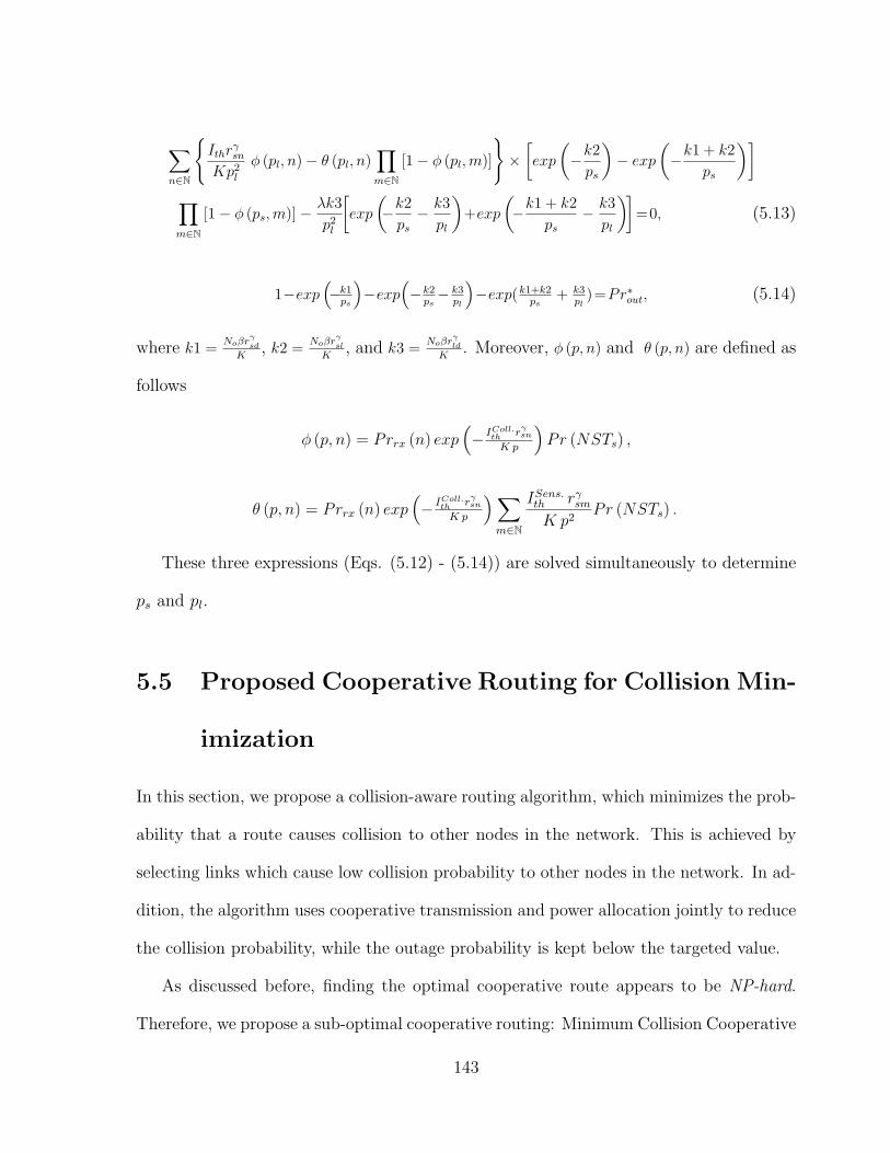
∑n∈N

Ithr

γsn

Kp2l


[1− φ (pl,m)]

×[exp

(−k2

ps

)− exp

(−k1 + k2

ps

)]∏m∈N

[1− φ (ps,m)]− λk3

p2l

[exp

(−k2

ps− k3

pl

)+exp

(−k1 + k2

ps− k3

pl

)]=0, (5.13)

1−exp(−k1ps

)−exp

(−k2ps− k3

pl

)−exp(k1+k2

ps+ k3

pl)=Pr∗out, (5.14)

where k1 =Noβr

γsd

K, k2 =

Noβrγsl

K, and k3 =

Noβrγld

K. Moreover, φ (p, n) and θ (p, n) are defined as

follows


K p

)Pr (NSTs) ,


K p

)∑m∈N

ISens.th rγsmK p2

Pr (NSTs) .

These three expressions (Eqs. (5.12) - (5.14)) are solved simultaneously to determine

ps and pl.

5.5 Proposed Cooperative Routing for Collision Min-

imization

In this section, we propose a collision-aware routing algorithm, which minimizes the prob-

ability that a route causes collision to other nodes in the network. This is achieved by

selecting links which cause low collision probability to other nodes in the network. In ad-

dition, the algorithm uses cooperative transmission and power allocation jointly to reduce

the collision probability, while the outage probability is kept below the targeted value.

As discussed before, finding the optimal cooperative route appears to be NP-hard.

Therefore, we propose a sub-optimal cooperative routing: Minimum Collision Cooperative

143

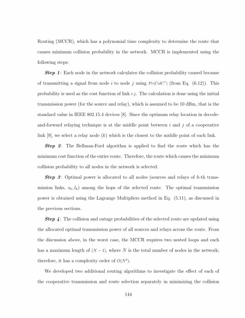
Routing (MCCR), which has a polynomial time complexity to determine the route that

causes minimum collision probability in the network. MCCR is implemented using the

following steps:

Step 1 : Each node in the network calculates the collision probability caused because

of transmitting a signal from node i to node j using Pr(Coll.C) (from Eq. (6.12)). This

probability is used as the cost function of link i-j. The calculation is done using the initial

transmission power (for the source and relay), which is assumed to be 10 dBm, that is the

standard value in IEEE 802.15.4 devices [8]. Since the optimum relay location in decode-

and-forward relaying technique is at the middle point between i and j of a cooperative

link [9], we select a relay node (k) which is the closest to the middle point of each link.

Step 2 : The Bellman-Ford algorithm is applied to find the route which has the

minimum cost function of the entire route. Therefore, the route which causes the minimum

collision probability to all nodes in the network is selected.

Step 3 : Optimal power is allocated to all nodes (sources and relays of h-th trans-

mission links, sh, lh) among the hops of the selected route. The optimal transmission

power is obtained using the Lagrange Multipliers method in Eq. (5.11), as discussed in

the previous sections.

Step 4 : The collision and outage probabilities of the selected route are updated using

the allocated optimal transmission power of all sources and relays across the route. From

the discussion above, in the worst case, the MCCR requires two nested loops and each

has a maximum length of (N − 1), where N is the total number of nodes in the network;

therefore, it has a complexity order of O(N2).

We developed two additional routing algorithms to investigate the effect of each of

the cooperative transmission and route selection separately in minimizing the collision

144

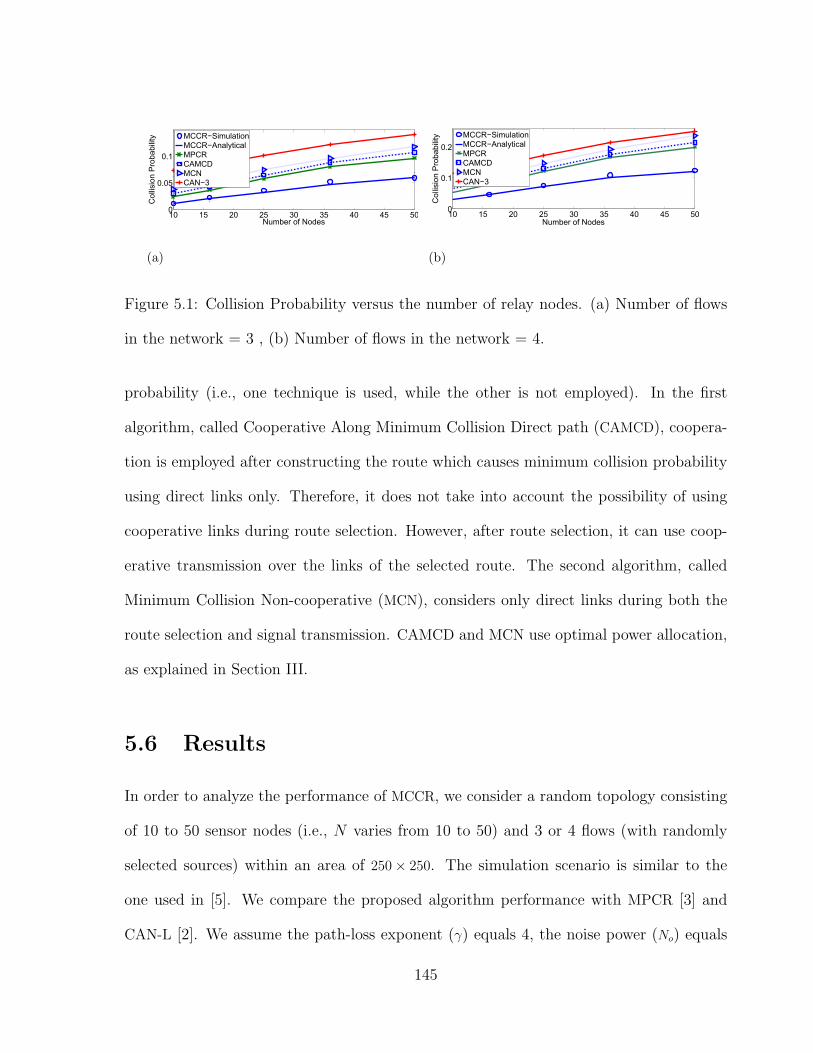
(a)

10 15 20 25 30 35 40 45 500

0.05

0.1

Number of Nodes

Col

lisio

n Pr

obab

ility

MCCR−SimulationMCCR−AnalyticalMPCRCAMCDMCNCAN−3

(b)

10 15 20 25 30 35 40 45 500

0.1

0.2

Number of Nodes

Col

lisio

n Pr

obab

ility


Figure 5.1: Collision Probability versus the number of relay nodes. (a) Number of flows

in the network = 3 , (b) Number of flows in the network = 4.

probability (i.e., one technique is used, while the other is not employed). In the first

algorithm, called Cooperative Along Minimum Collision Direct path (CAMCD), coopera-

tion is employed after constructing the route which causes minimum collision probability

using direct links only. Therefore, it does not take into account the possibility of using

cooperative links during route selection. However, after route selection, it can use coop-

erative transmission over the links of the selected route. The second algorithm, called

Minimum Collision Non-cooperative (MCN), considers only direct links during both the

route selection and signal transmission. CAMCD and MCN use optimal power allocation,

as explained in Section III.

5.6 Results

In order to analyze the performance of MCCR, we consider a random topology consisting

of 10 to 50 sensor nodes (i.e., N varies from 10 to 50) and 3 or 4 flows (with randomly

selected sources) within an area of 250× 250. The simulation scenario is similar to the

one used in [5]. We compare the proposed algorithm performance with MPCR [3] and

CAN-L [2]. We assume the path-loss exponent (γ) equals 4, the noise power (No) equals

145

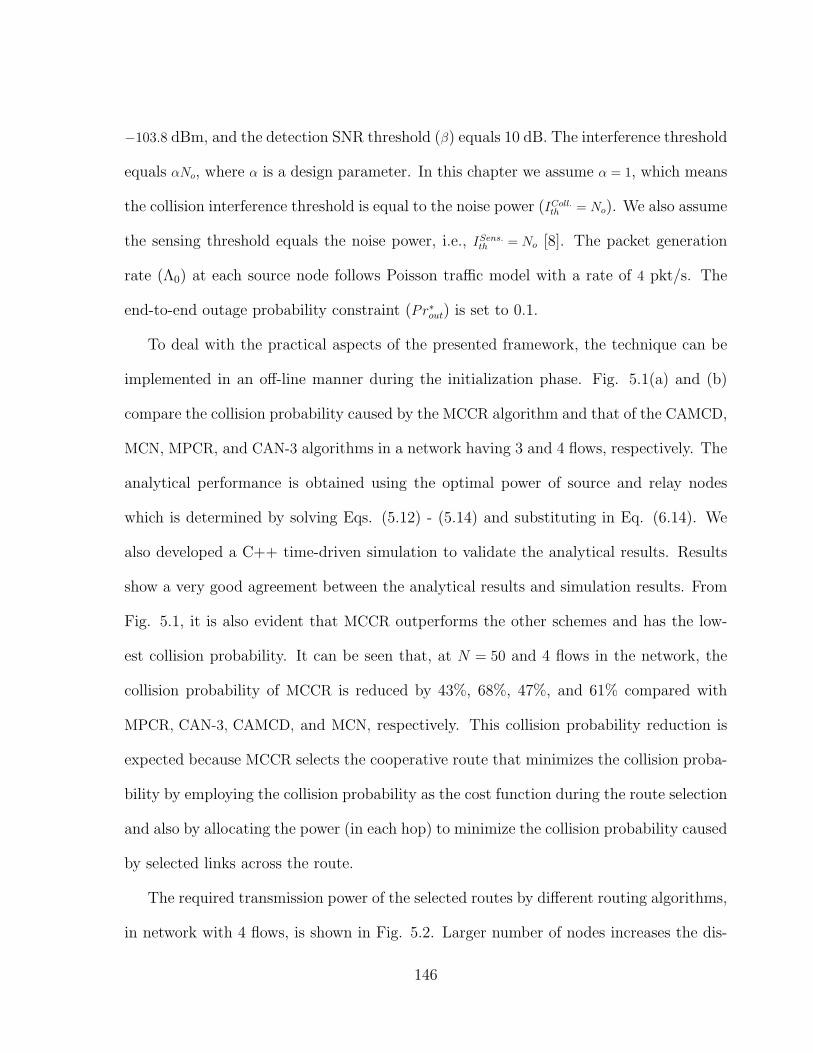
−103.8 dBm, and the detection SNR threshold (β) equals 10 dB. The interference threshold

equals αNo, where α is a design parameter. In this chapter we assume α = 1, which means

the collision interference threshold is equal to the noise power (IColl.th = No). We also assume

the sensing threshold equals the noise power, i.e., ISens.th = No [8]. The packet generation

rate (Λ0) at each source node follows Poisson traffic model with a rate of 4 pkt/s. The

end-to-end outage probability constraint (Pr∗out) is set to 0.1.

To deal with the practical aspects of the presented framework, the technique can be

implemented in an off-line manner during the initialization phase. Fig. 5.1(a) and (b)

compare the collision probability caused by the MCCR algorithm and that of the CAMCD,

MCN, MPCR, and CAN-3 algorithms in a network having 3 and 4 flows, respectively. The

analytical performance is obtained using the optimal power of source and relay nodes

which is determined by solving Eqs. (5.12) - (5.14) and substituting in Eq. (6.14). We

also developed a C++ time-driven simulation to validate the analytical results. Results

show a very good agreement between the analytical results and simulation results. From

Fig. 5.1, it is also evident that MCCR outperforms the other schemes and has the low-

est collision probability. It can be seen that, at N = 50 and 4 flows in the network, the

collision probability of MCCR is reduced by 43%, 68%, 47%, and 61% compared with

MPCR, CAN-3, CAMCD, and MCN, respectively. This collision probability reduction is

expected because MCCR selects the cooperative route that minimizes the collision proba-

bility by employing the collision probability as the cost function during the route selection

and also by allocating the power (in each hop) to minimize the collision probability caused

by selected links across the route.

The required transmission power of the selected routes by different routing algorithms,

in network with 4 flows, is shown in Fig. 5.2. Larger number of nodes increases the dis-

146

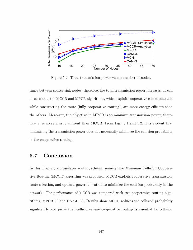
10 15 20 25 30 35 40 45 50

10−2

10−1

Number of Nodes

Tota

l Tra

nsm

issi

on P

ower

(Wat

t)


Figure 5.2: Total transmission power versus number of nodes.

tance between source-sink nodes; therefore, the total transmission power increases. It can

be seen that the MCCR and MPCR algorithms, which exploit cooperative communication

while constructing the route (fully cooperative routing), are more energy efficient than

the others. Moreover, the objective in MPCR is to minimize transmission power; there-

fore, it is more energy efficient than MCCR. From Fig. 5.1 and 5.2, it is evident that

minimizing the transmission power does not necessarily minimize the collision probability

in the cooperative routing.

5.7 Conclusion

In this chapter, a cross-layer routing scheme, namely, the Minimum Collision Coopera-

tive Routing (MCCR) algorithm was proposed. MCCR exploits cooperative transmission,

route selection, and optimal power allocation to minimize the collision probability in the

network. The performance of MCCR was compared with two cooperative routing algo-

rithms, MPCR [3] and CAN-L [2]. Results show MCCR reduces the collision probability

significantly and prove that collision-aware cooperative routing is essential for collision

147

probability minimization.

REFERENCES



pp. 3062–3080, Dec. 2004.

[2] A. E. Khandani, J. Abounadi, E. Modiano, and L. Zheng, “Cooperative routing in

static wireless networks,” IEEE Trans. Wireless Commun., vol. 55, no. 11, pp. 2185–

2192, Nov. 2007.



Oct. 2008.

[4] L. Wang, K. Wu, and M. Hamdi, “Combating hidden and exposed terminal problems

in wireless networks,” IEEE Trans. Wireless Commun., vol. 11, no. 11, pp. 4204–4213,

Nov. 2012.

[5] J. Zhang and Q. Zhang, “Cooperative routing in multi-source multi-destination multi-

hop wireless networks,” in Proc. IEEE INFOCOM, Apr. 2008, pp. 306–310.

148

[6] B. Han, J. Li, J. Su, and J. Cao, “Self-supported cooperative networking for emergency

services in multi-hop wireless networks,” IEEE J. Sel. Areas Commun., vol. 30, no. 2,

pp. 450–457, Feb. 2012.

[7] S. Rao, Engineering Optimization: Theory and Practice. Wiley, 2009.




communication in wireless networks,” in Proc. IEEE WCNC, Apr. 2013, pp. 4724–

4729.

149

Chapter 6

Optimal and Near-Optimal

Cooperative Routing and Power

Allocation for Collision Minimization

in Wireless Sensor Networks

6.1 Abstract

Cooperative communication has gained much interest due to its ability to exploit the

broadcast nature of the wireless medium to mitigate multipath fading. There has been

considerable research on how cooperative transmission can improve the performance of

the network physical layer. Recently, researchers have started to take into consideration

cooperative transmission in routing and there has been a growing interest in developing

cooperative routing protocols. Most of the existing cooperative routing algorithms are

150

designed to reduce the energy consumption; however, packet collision minimization using

cooperative routing has not been addressed yet. This chapter presents an optimization

framework to minimize collision probability using cooperative routing in wireless sensor

networks. We develop a mathematical model and formulate the problem as a large-scale

Mixed Integer Non-Linear Programming problem. We also propose a solution based on

the branch and bound algorithm augmented with reducing the search space. The proposed

strategy builds up the optimal routes from each source to the sink node by providing the

best set of hops in each route, the best set of relays, and the optimal power allocation for

the cooperative transmission links. To reduce the computational complexity, we propose a

near-optimal cooperative routing algorithm in which we solve the problem by decoupling

the power allocation problem and the route selection problem. Therefore, the problem

is formulated by an Integer Non-Linear Programming, which is solved using branch and

bound space reduced method. The simulation results reveal the presented algorithms can

significantly reduce the collision probability compared with existing schemes.

6.2 Introduction

Cooperative communication has emerged as a promising approach for mitigating wireless

channel fading and improving the reliability of wireless networks by allowing nodes to

collaborate with each other. Nodes in cooperative communication help each other with

information transmission by exploiting the broadcasting nature of wireless communication

[1]. In a cooperative transmission scheme, neighboring nodes are exploited as relay nodes,

in which they cooperate with the transmitter-receiver pair to deliver multiple copies of

a packet to the receiver node through independent fading channels. The idea behind

151

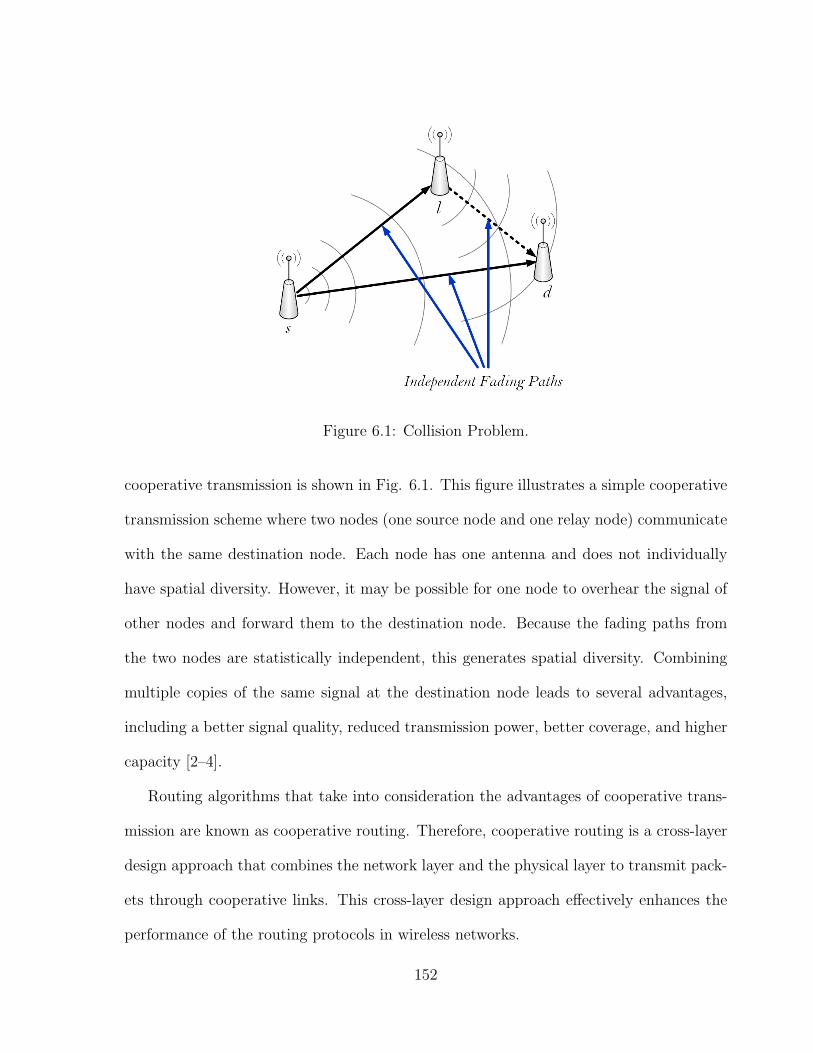
Figure 6.1: Collision Problem.

cooperative transmission is shown in Fig. 6.1. This figure illustrates a simple cooperative

transmission scheme where two nodes (one source node and one relay node) communicate

with the same destination node. Each node has one antenna and does not individually

have spatial diversity. However, it may be possible for one node to overhear the signal of

other nodes and forward them to the destination node. Because the fading paths from

the two nodes are statistically independent, this generates spatial diversity. Combining

multiple copies of the same signal at the destination node leads to several advantages,

including a better signal quality, reduced transmission power, better coverage, and higher

capacity [2–4].

Routing algorithms that take into consideration the advantages of cooperative trans-

mission are known as cooperative routing. Therefore, cooperative routing is a cross-layer

design approach that combines the network layer and the physical layer to transmit pack-

ets through cooperative links. This cross-layer design approach effectively enhances the

performance of the routing protocols in wireless networks.

152

Cooperative routing was introduced by Khandani et al. [5] and the authors also showed

that the problem of finding the optimum cooperative route is NP-Hard. In the past few

years, significant progress has been made on the design and development of coopera-

tive routing protocols. In [6], we presented a comprehensive survey of existing coopera-

tive routing techniques together with the highlights of the performance of each strategy.

While many efficient sub-optimal cooperative routing algorithms are proposed in the lit-

erature, only a few studies have focused on optimal cooperative routing. Sub-optimal

cooperative routing algorithms can be divided into two categories. The first category of

cooperation-based routing algorithms, namely Cooperative Along Shortest-Path (such as

the proposed algorithms in [5,7]) is implemented by finding the shortest-path route first,

and then building the cooperative route based on the shortest path. The main idea of

algorithms in this category is to use cooperative transmission to improve performance

along the selected non-cooperative route. However, the optimal cooperative route might

be completely different from the non-cooperative shortest path. Therefore, the merits of

cooperative routing are not fully exploited if cooperation is not taken into account while

selecting the route. One of the heuristic cooperative routing algorithms presented in [5] is

called the Cooperative Along Non-cooperative (CAN-L) algorithm with the objective of

minimizing total transmitted power. The basic idea is to run a non-cooperative shortest

path first, and then to use cooperative transmission by the last L nodes along the non-

cooperative path. The algorithms in the second category, Cooperative Based Path (e.g.,

the proposed algorithms in [8, 9]), address the above problem by exploiting cooperative

routing during the route selection process. However, the algorithms in this category are

not optimal due to the following reasons: (1) they employ sub-optimal approaches in the

relay node selection [9], power allocation [8], or route selection [10] and (2) they utilize

153

optimal relay node selection, resource allocation, and route selection but not jointly (as

will be discussed in detail in Section 6.5), such as the algorithm in [2]. Authors in [8]

presented an algorithm called Minimum Power Cooperative Routing (MPCR). The algo-

rithm finds the route that minimizes the total transmission power. MPCR makes routing

decisions by assuming the cooperative transmission is also available for each link. In [9]

the authors proposed the EP-H1 algorithm. The EP-H1 algorithm considers the two-

stage cooperation model to find the route that consumes minimum energy. In the fist

stage the transmitter node broadcasts the message to its neighbors. In the second stage

every node that has successfully decoded the message will join the transmitter node to

form a cooperative transmitting set. The transmitting set cooperatively transmits the

message to a receiver node using equal power. The power allocation vector minimizes the

total amount of consumed energy.

The main objective of cooperative routing in all proposed schemes, either the optimal

or sub-optimal cooperative routing algorithms, is to save energy while guaranteeing a

certain QoS. However, packet collision minimization has not been taken into account in

existing cooperative routing algorithms.

Interactions among multiple neighboring flows may lead to the hidden and exposed

node problems which cause packet collision. In general, cooperative routing can improve

the performance due to the more robust links and less power consumption. However,

cooperative routing causes extra packet transmission by the relays. Therefore, the gain of

a cooperative routing algorithm with multiple flows is different from the one with a single

flow, especially in terms of the packet collision probability. There are only a few papers,

such as [11–13], that considered multiple flows in cooperative routing. In [11] collision is

brought into attention by defining a contention graph, where a set of transmitting nodes

154

coordinates their transmissions to a set of receiving nodes. The algorithm approaches the

non-cooperative protocol when network congestion emerges. Moreover, the congestion

problem of cooperative routing in [12] is solved in the MAC layer. In [13], we proposed

Minimum Collision Cooperative Routing (MCCR) algorithm by combining cooperative

transmission, optimal power allocation, and route selection. However, the proposed al-

gorithm is a sub-optimal routing due to the following reasons; (1) the optimal power

allocation technique is decoupled from the optimal route selection and (2) a sub-optimal

approach is employed in the relay node selection and relay nodes are selected as the node

closest to the middle point of the transmitter and receiver nodes of each link.

In WSNs, upon the detection of an event, packet traffic load in some spots may get

intensified, resulting in a high packet collision rate and consequently, packet loss. To solve

this problem, we develop a mathematical characterization for the collision probability in

cooperative routing. The presented framework demonstrates the exact formulation for

the optimal relay node and optimal power allocation set, and the joint use of optimal

power, relay node allocation, and path selection. The final problem formulation is in

the form of Mixed Integer Non-linear Programming (MINLP). We propose a solution

procedure based on the branch and bound method augmented with the effective space

reduction method. The computational complexity of the algorithm for solving these

problems grows exponentially with the number of binary variables. Due to the high

complexity of the problem, one cannot obtain optimal solutions within reasonable time

for the large network topologies. Therefore, one needs to resort to the heuristic approach.

We present a heuristic near-optimal algorithm for the formulated problem by decoupling

the optimal transmission power allocation from the route selection; we solve the INLP in

the first phase and apply optimum power in the second phase.

155

To the best of our knowledge, there is no framework which can accurately characterize

the collision probability in the cooperative network and minimize the collision problem

employing cooperative routing. Overall, the main contribution of this chapter includes

the following:

1. The collision problem in WSNs is formally defined and formulated. The traffic load

per node in cooperative transmission is also explored.

2. An MINLP model, employing the cooperative routing, is presented to minimize the

collision problem subject to the outage probability constraint.

3. The MINLP solution serves as a benchmark for evaluating the quality of the solu-

tions obtained by any sub-optimal algorithm for this problem.

4. The obtained solution applies a joint optimization approach for power allocation,

relay node assignment, and path selection which are the main optimization issues

in cooperative routing.

5. Moreover, near-optimal algorithms are proposed by separating one of the optimiza-

tion variable decisions, i.e., optimal transmission power, from the other optimization

variables.

6. Our proposed algorithms find good solutions which ensure minimizing collision prob-

ability compared to the existing cooperative routing algorithms.

The remainder of this chapter is organized as follows. In Section 6.3, we illustrate

the system model and formulate our optimization task. In Section 6.4, we develop a

mathematical model and we formulate the problem to minimize collision probability by

156

optimizing the relay node assignment, power allocation and path selection jointly. In

Section 6.5, we propose the optimal solution to the problem. In Section 6.6, a near-

optimal cooperative routing algorithm is presented. Simulation results and performance

evaluations are given in Section 6.7. Finally, we conclude the chapter in Section 6.8.

6.3 System Model

We consider a WSN, where source nodes communicate with the destination nodes (or

sink nodes) via cooperative routing. Let hij and nij represent the Rayleigh fading chan-

nel coefficient and the additive white Gaussian noise of the link between nodes i and j,

respectively. We assume that the distance-based attenuation follows the generic exponen-

tial path-loss model with an exponent γ [8].

In direct transmission, where a source (s) transmits its signal directly to the next

destination (d), the received signal at d is given by

ysd =

√pDs Kr



is a constant that depends on the characteristics of the transmitter, the receiver, and

channel (e.g., the frequency and the antenna gain), rsd is the distance between the two

nodes (s and d), and u is the transmitted data with a unity power.

The criterion for a good detection is that the received signal-to-noise-ratio (SNR)

must be greater than the detection threshold (β). Outage is defined as the status when

the receiver is unable to detect data u. Hence, a link is considered to be in outage if

the received SNR falls below β. Thus, the outage probability, when direct transmission

157

is only used, PrDout, is defined as Pr(SNRsd < β). It can be easily shown that the

power that minimizes the collision probability subject to the outage probability constraint

(PrDout ≤ Pr∗out) is given by

pDs = − βNorγsd

K ln(1− Pr∗out), (6.2)


power.

In cooperative transmission, the employed system model is similar to that used in [8].

As shown in Fig. 6.1, a cooperative link consists of three nodes: source (s), destination

(d), and a potential relay node (l). The relaying technique used in this study is the

incremental adaptive decode-and-forward. With this technique, the source sends its signal

to the destination using the direct link. If the destination is unable to detect the signal

using the direct link, the relay forwards the signal to the destination (provided that the

relay was able to detect the signal). If the relay is unable to detect the signal, it remains

silent and the destination will rely on the direct signal only. For cooperative transmission,

the received signals from s at d and l can be respectively expressed as

ysd =

√pCs Kr


ysl =

√pCs Kr



the relay forwards the signal to the destination, the received signal at the destination from

the relay node can be expressed as yld =√pCl Kr

−γld hldu+nld, where pCl is the transmission

power of the relay node. In this case, the destination detects the signal using the relay

signal only. Although combining schemes such as maximum ratio combining are more

158

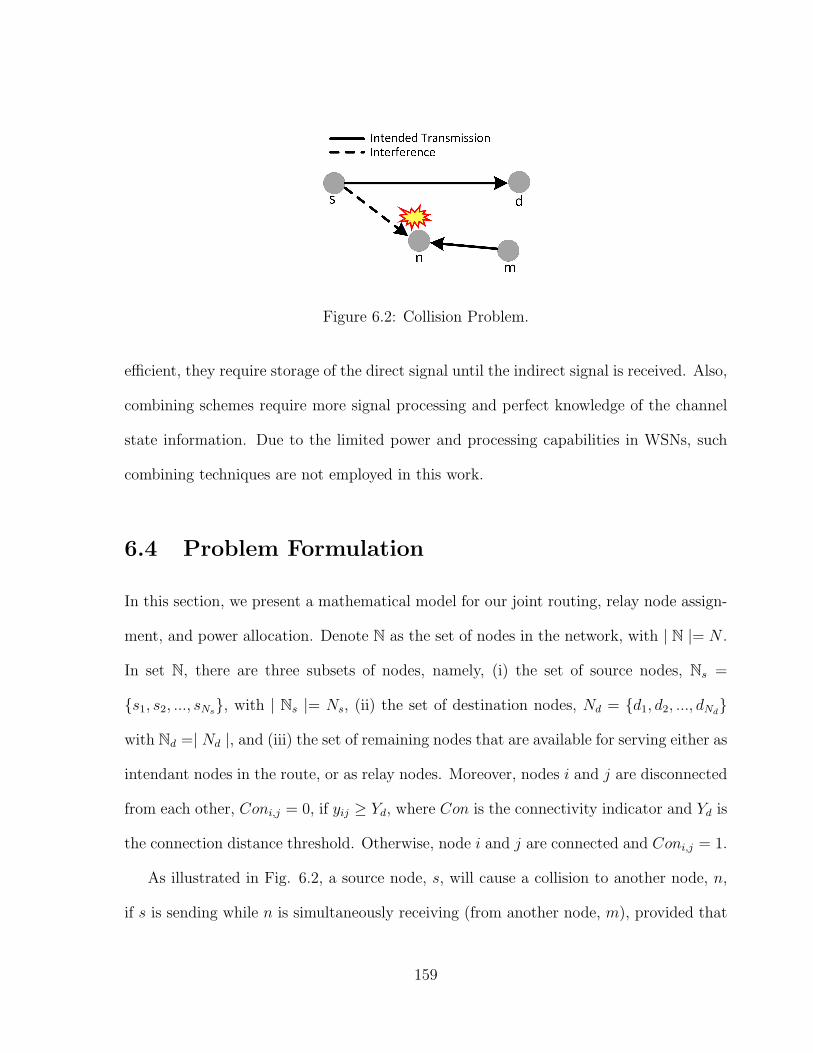
Figure 6.2: Collision Problem.

efficient, they require storage of the direct signal until the indirect signal is received. Also,

combining schemes require more signal processing and perfect knowledge of the channel

state information. Due to the limited power and processing capabilities in WSNs, such

combining techniques are not employed in this work.

6.4 Problem Formulation

In this section, we present a mathematical model for our joint routing, relay node assign-

ment, and power allocation. Denote N as the set of nodes in the network, with | N |= N .

In set N, there are three subsets of nodes, namely, (i) the set of source nodes, Ns =

s1, s2, ..., sNs, with | Ns |= Ns, (ii) the set of destination nodes, Nd = d1, d2, ..., dNd

with Nd =| Nd |, and (iii) the set of remaining nodes that are available for serving either as

intendant nodes in the route, or as relay nodes. Moreover, nodes i and j are disconnected

from each other, Coni,j = 0, if yij ≥ Yd, where Con is the connectivity indicator and Yd is

the connection distance threshold. Otherwise, node i and j are connected and Coni,j = 1.

As illustrated in Fig. 6.2, a source node, s, will cause a collision to another node, n,

if s is sending while n is simultaneously receiving (from another node, m), provided that

159

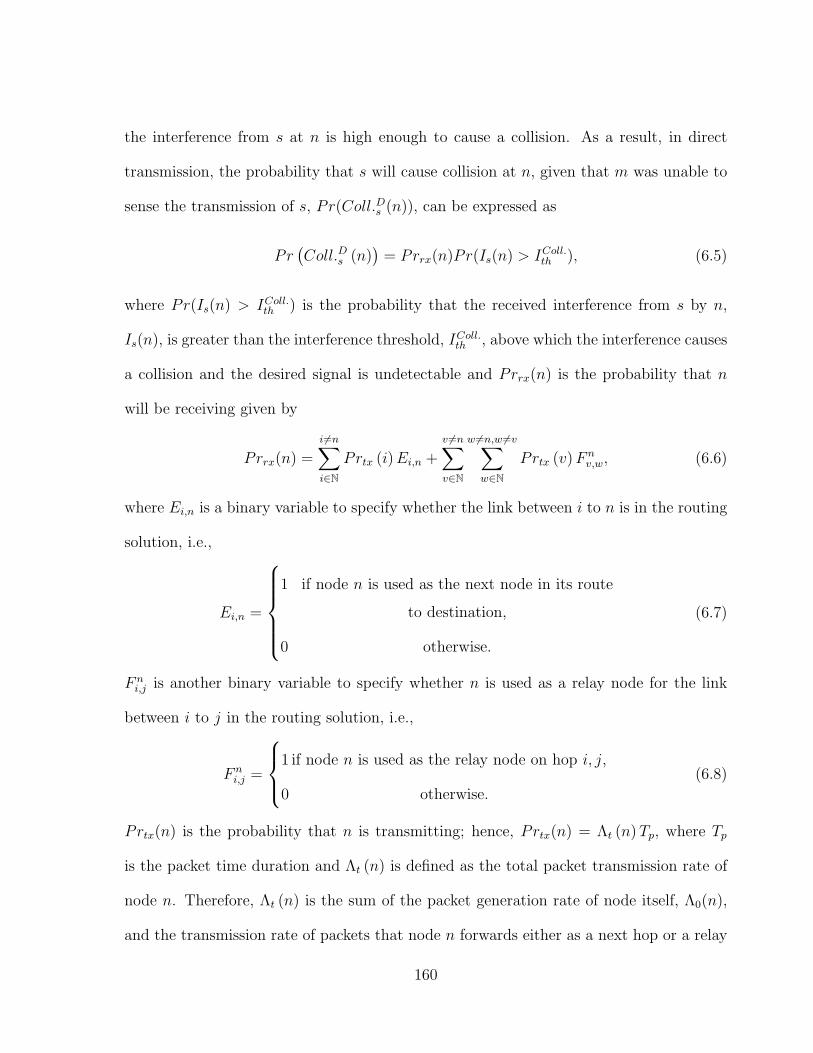
the interference from s at n is high enough to cause a collision. As a result, in direct

transmission, the probability that s will cause collision at n, given that m was unable to

sense the transmission of s, Pr(Coll.Ds (n)), can be expressed as

Pr(Coll.Ds (n)

)= Prrx(n)Pr(Is(n) > IColl.th ), (6.5)

where Pr(Is(n) > IColl.th ) is the probability that the received interference from s by n,

Is(n), is greater than the interference threshold, IColl.th , above which the interference causes

a collision and the desired signal is undetectable and Prrx(n) is the probability that n

will be receiving given by

Prrx(n) =

i6=n∑i∈N

Prtx (i)Ei,n +

v 6=n∑v∈N

w 6=n,w 6=v∑w∈N

Prtx (v)F nv,w, (6.6)

where Ei,n is a binary variable to specify whether the link between i to n is in the routing

solution, i.e.,

Ei,n =

1 if node n is used as the next node in its route

to destination,

0 otherwise.

(6.7)

F ni,j is another binary variable to specify whether n is used as a relay node for the link

between i to j in the routing solution, i.e.,

F ni,j =

1 if node n is used as the relay node on hop i, j,

0 otherwise.

(6.8)

Prtx(n) is the probability that n is transmitting; hence, Prtx(n) = Λt (n)Tp, where Tp

is the packet time duration and Λt (n) is defined as the total packet transmission rate of

node n. Therefore, Λt (n) is the sum of the packet generation rate of node itself, Λ0(n),

and the transmission rate of packets that node n forwards either as a next hop or a relay

160

node, thus,

Λt(n) = Λ0(n) +

m6=n∑m∈N

Λt(m)Em,n

(Pr (SNRmn > β) +

Pr (SNRmn < β)

l 6=n,l 6=m∑l∈N

Pr (SNRml > β)Pr (SNRln < β)

+

k 6=n,k 6=m∑k∈N

F nm,kPr (SNRmk < β) (SNRmn > β)

, (6.9)

where SNRmn is the SNR of the link between node m and node n.

Employing Carrier Sense Multiple Access with Collision Avoidance (CSMA-CA) mech-

anism for channel access, nodes that are within the sensing range of a transmitter are

inhibited from transmitting. Therefore, the probability that s will cause a collision to one

or more nodes in the network is given by

Pr(Coll.Ds ) =(

1−∏n∈N

(1− Pr

(Coll.Ds (n)

)) )Pr (NSTs) , (6.10)

where Pr(NSTs) is the average probability of not sensing transmission of s by a node

that has traffic to send to n, thus,

Pr (NSTs) =∑m∈N

Pr(Is(m) < ISens.th )(Prtx(m)Em,n+

k 6=m,n∑k∈N

Prtx(k)F km,nPr (SNRmn < β)Pr (SNRkn > β)

), (6.11)

where ISens.th is the carrier sensing threshold above which the channel is deemed busy.



caused by the source, Pr(Coll.Ds ), if the direct signal (from the source) is detectable at

the destination or if the relay node is unable to detect the source signal. Otherwise,

collision happens by either the source or the relay; hence, the collision probability is the

161

probability of the union of two events: 1) collision caused by the source and 2) collision

caused by the relay. Thus, the per node collision probability caused by the cooperative

transmission (from s and l) to all other nodes in the network is given by

Pr(Coll.Cs,l

)= Pr(Coll.Ds )[

Pr (SNRsd > β) + Pr (SNRsd < β)Pr (SNRsl > β)]+[

1−(1− Pr(Coll.Ds )

)(1− Pr(Coll.Dl )

)]Pr(SNRsd < β)Pr(SNRsl > β). (6.12)

Inserting the exponential distribution due to the Rayleigh fading and after mathemat-

ical manipulation, Eq. (6.12) can be rewritten as in Eq. (6.13).

Pr(Coll.Cs,l

)=

(1−

i6=s∏i∈N

[1− Prrx (i) exp

(−Ith r

γsi

K ps

) j 6=s,j 6=i∑j∈N

Prtx (j)

(1− exp

(−I′

th rγsj

K ps

))])

+

(1−

i6=s∏i∈N

[1− Prrx (i) exp

(−Ith r

γsi

K pl

) j 6=sj 6=i∑j∈N

Prtx (j)

(1− exp

(−I′

th rγsj

K pl

))])(

1− exp(−No βd r

γsd

Kps

))∗ exp

(−No βd r

γsl

Kps

)−

(1−

i6=s∏i∈N

[1− Prrx (i) exp

(−Ith r

γsi

K ps

) j 6=s,j 6=i∑j∈N

Prtx (j)

(1− exp

(−I′

th rγsj

K ps

))])(

1−i6=s∏iinN

[1− Prrx (i) exp

(−Ith r

γsi

K pl

) j 6=s,j 6=i∑j∈N

Prtx (j)

(1− exp

(−I′

th rγsj

K pl

))])(

1− exp(−No βd r

γsd

Kps

))exp

(−No βd r

γsl

Kps

)(6.13)

Therefore, the probability that the entire route causes collision can be expressed as

Pr(Coll.route) = 1−H∏h=1

(1− Pr

(Coll.Csh,lh (h)

)), (6.14)

where h is the hop number and H is the total number of hops in the route.

162

In a cooperative transmission link with incremental adaptive decode-and-forward re-

laying, outage probability is given by

PrCout= Pr(SNRsd < β)Pr(SNRsl < β) (6.15)

+Pr(SNRsd < β)Pr(SNRsl > β)Pr(SNRld < β).

Employing the exponential SNR in Eq. (6.15), outage probability of a cooperative

link can be expressed as

PrCout = 1− exp(−k1ps

)− exp

(−k2ps− k3

pl

)− exp(k1+k2

ps+ k3

pl), (6.16)

where k1 =Noβr

γsd

K, k2 =

Noβrγsl

K, and k3 =

Noβrγld

K.

In addition to that, the end-to-end outage probability of a certain route is defined as

the probability that outage takes place in one of the H hops of the route, i.e.,


(1− PrCout (h)

), (6.17)

where PrCout (h) is the outage probability of the h-th link in the route.

The goal of the algorithm is to find the route from each source to the sink such that

each route minimizes the collision probability per node due to the route to other nodes

in the network, while satisfying the end-to-end outage probability constraint. Therefore,

163

the optimization problem can be formulated as below

Min.psh , plh , Ei,j , F

ki,j

CollT , (6.18)

s.t. Prout(router) ≤ Pr∗out, ∀r ∈ Ns

C1 : 1 ≤∑i∈N

j 6=i∑j∈N

Ei,j +∑i∈N

j 6=i∑j∈N

k 6=i,k 6=j∑k∈N

F ki,j ≤ 2Ns (N − 1) ,

C2 : Ei,j − F ki,j ≥ 0, ∀i, j, k ∈ N i 6= j 6= k

C3 : Ei,j −k 6=i∑k∈N

Ej,k ≥ 0,

C4 :

i6=D∑i∈N

Ei,D ≥ 1,

C5 :

i6=D∑i∈N

ES,i ≥ 1,

where psh , plh , Ei,j, and F ki,j are the optimization variable. CollT is the objective function,

which is the total collision probability per node in the network and can be expressed as

CollT = 1−Ns∏r=1

(1− Pr(Coll.router)). (6.19)

As explained earlier, each node in a cooperative routing can receive data from the

previous node and can work either as the relay node or the next hop. Constraint C1 in

(6.18) forces the range for the number of links involved in the source-destination paths in

the network with Ns source nodes (i.e., Ns flows in the network). A cooperative relay node

may be assigned to hop (i, j) only if the hop is included in the path solution. Otherwise,

no relay node will be assigned to that hop (i, j); C2 in Eq. (6.18) characterizes this

constraint. Constraint C2 also holds when j is not a next hop and in that case all E

variables in (6.18) are equal to zero. Constraint C3 formulates the flow balance at an

intermediate node along the path between each source, si, and the destination node, D.

164

Moreover, the destination node must be reached and each source node must transmit data

to some other nodes. These constraints are expressed by C4 and C5, respectively.

Obviously, (6.18) is a Mixed Integer Non-Linear Programming problem, since the

binary variables (Ei,j, Fki,j) and real variables (psh , plh) are involved in the non-linear

objective and the constraints.

Lemma 1. The minimum collision cooperative routing problem is NP-Hard.

The proof of Lemma 1 is given in the Appendix.

6.5 Proposed Solution Procedure

The Branch and Bound (BnB) algorithm is by far the most widely used tool for solving

integer optimization problems. Obviously, the optimal value of cost function in a contin-

uous linear relaxation of a problem will always be a lower bound on the optimal value

of the cost function. Moreover, in any minimization, any feasible point always specifies

an upper bound on the optimal cost function value. The idea of the BnB is to utilize

these observations to subdivide MINLP‘s feasible region into more-manageable subdivi-

sions and then, if required, to further partition the subdivisions. These subdivisions make

a so-called enumeration tree whose branches can be pruned in a systematic search for the

global optimum.

6.5.1 Branch and Bound Space Reduced algorithm

We enhance the BnB algorithm and develop a BnB Space Reduced algorithm to solve the

MINLP. This proposed algorithm reduces the BnB area of a search and implements the

165

BnB relaxation and separation strategy to solve the problem.

The pseudocode of the proposed framework, using the BnB-Space Reduced, is de-

scribed in Table 1. In this algorithm, Ω represents optimization problem set and Ω∗ de-

notes the global minimum of the cost function CollT . Therefore, the algorithm provides a

(1- ε) optimal solution Ωε, which means Ωε is close enough to Ω∗ such that Ω∗ ≥ (1− ε)Ω.

Initially, Ω includes the original problem, i.e., CollT denoted by ω0. A lower bound of

the cost function is first derived through solving a linear relaxation of CollT denoted by

(BL) (line 3 in Table 1. Construction of the linear relaxation is described in the next sub-

section. Since any feasible solution of ω can serve as an upper bound, the one obtained

by rounding under the satisfaction of all constraints is used and denoted as BU .

The process of finding the lower and upper bound for the cost function, is called

bounding. If the derived upper and lower bounds are within the ε-vicinity of each other, the

algorithm terminates (line 10, 11). Otherwise, it divides the feasible region of the problem

into two narrower subsets (branching step), and the problem ω will be replaced with two

subproblems ω1 and ω2 constructed by branching binary variable Ei,j, respectively (see

line 17). Simultaneously, other variables are fixed according to the constraints in Eq.

(6.18).

The developed feature of BnB, reduces the feasible integer variable space. In this phase

of the algorithm, all subsets that include the disconnected integer variables (i.e., discon-

nected next hop (Ei,j = 1&Coni,j = 0) or disconnected relay node(F ki,j = 1&Coni,k = 0

or Conk,j = 0) are removed and the subsets area of search is reduced.

Through an iterative branching procedure, subsets are further divided into smaller

ones to build the enumeration tree. The structure of the enumeration tree allows the

algorithm to remove some branches and search for the solution in a very effective way.

166

Moreover, narrowing down the subsets of the optimization variables makes the linear

relaxations tighter (i.e., increases BL) and provides the next local search processes with

a closer starting point to the optimal solution (i.e., reduces BU). Hence, the gap between

BL and BU is reduced as the process continues. More precisely, the global lower bound

BL is updated in each iteration, in order to contain the minimum of the lower bounds

of all subsets (lines 5, 6). The global upper bound BU is also updated at each iteration

(lines 8, 9) and the branches with a lower bound greater than (1− ε)BU are pruned (line

13). This approach is continued until the difference between the global lower and upper

bounds satisfy the accuracy ε (lines 10, 11). Clearly, we may lose the global optimum

by pruning the branches. However, if the global optimum is in a pruned branch with

the lower bound is BLω , then Ω∗ ≥ BLω , and consequently, Ω∗ ≥ (1 − ε)BU . Therefore,

the current best feasible solution with objective value BU is already an (1 − ε) optimal

solution, and the optimality is still guaranteed (1− ε). In fact, this guarantee is the key

feature of the algorithm, which makes it very effective in solving the MINLP.

6.5.2 A lower bound for the collision problem

To obtain the exact solution using a branch-and-bound algorithm in a reasonable com-

putation time, computation of the lower bound of the cost of each branch are important.

The stronger bound decreases the number of enumerations for searching the most promis-

ing branch. In order to derive the lower bound of the collision problem the linearization

technique along with relaxation of the integer variables are used and the non-linear ob-

jective and constraint are replaced by the linear-relaxed form. Firstly, we approximate

the exponential expression in the objective function (CollT ) and constraint in Eq. (6.17)

167

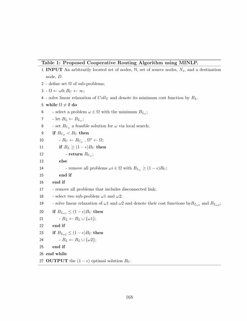
Table 1: Proposed Cooperative Routing Algorithm using MINLP.

1 INPUT An arbitrarily located set of nodes, N, set of source nodes, Ns, and a destination

node, D.

2 - define set Ω of sub-problems;

3 - Ω← ω0;BU ←∞;

4 - solve linear relaxation of CollT and denote its minimum cost function by BL.

5 while Ω 6= ∅ do6 - select a problem ω ∈ Ω with the minimum BLω ;

7 - let BL ← BLω ;

8 - set BUω a feasible solution for ω via local search;

9 if BUω < BU then

10 - BU ← BUω , Ω∗ ← Ω;

11 if BL ≥ (1− ε)BU then

12 - return BUω ;

13 else

14 - remove all problems ωi ∈ Ω with BLω ≥ (1− ε)BU ;

15 end if

16 end if

17 - remove all problems that includes disconnected link;

18 - select two sub-problem ω1 and ω2;

19 - solve linear relaxation of ω1 and ω2 and denote their cost functions byBLω1 and BLω2 ;

20 if BLω1 ≤ (1− ε)BU then

21 - BL ← BL ∪ ω1;22 end if

23 if BLω2 ≤ (1− ε)BU then

24 - BL ← BL ∪ ω2;25 end if

26 end while

27 OUTPUT the (1− ε) optimal solution BU .

168

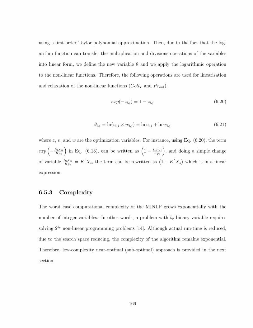
using a first order Taylor polynomial approximation. Then, due to the fact that the log-

arithm function can transfer the multiplication and divisions operations of the variables

into linear form, we define the new variable θ and we apply the logarithmic operation

to the non-linear functions. Therefore, the following operations are used for linearisation

and relaxation of the non-linear functions (CollT and Prout).

exp(−zi,j) = 1− zi,j (6.20)

θi,j = ln(vi,j × wi,j) = ln vi,j + lnwi,j (6.21)

where z, v, and w are the optimization variables. For instance, using Eq. (6.20), the term

exp(− Ithrsi

Kps

)in Eq. (6.13), can be written as

(1− Ithrsi

Kps

), and doing a simple change

of variable IthrsiKps

= K′Xs, the term can be rewritten as

(1−K ′Xs

)which is in a linear

expression.

6.5.3 Complexity

The worst case computational complexity of the MINLP grows exponentially with the

number of integer variables. In other words, a problem with br binary variable requires

solving 2br non-linear programming problems [14]. Although actual run-time is reduced,

due to the search space reducing, the complexity of the algorithm remains exponential.

Therefore, low-complexity near-optimal (sub-optimal) approach is provided in the next

section.

169

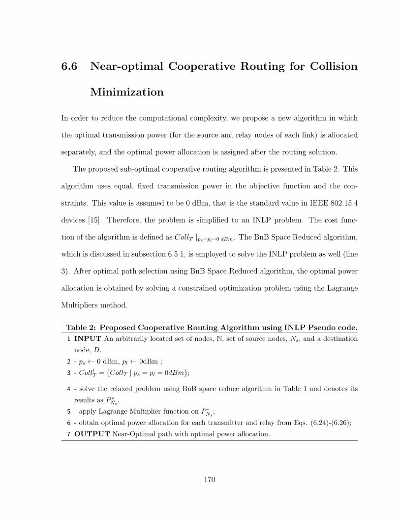
6.6 Near-optimal Cooperative Routing for Collision

Minimization

In order to reduce the computational complexity, we propose a new algorithm in which

the optimal transmission power (for the source and relay nodes of each link) is allocated

separately, and the optimal power allocation is assigned after the routing solution.

The proposed sub-optimal cooperative routing algorithm is presented in Table 2. This

algorithm uses equal, fixed transmission power in the objective function and the con-

straints. This value is assumed to be 0 dBm, that is the standard value in IEEE 802.15.4

devices [15]. Therefore, the problem is simplified to an INLP problem. The cost func-

tion of the algorithm is defined as CollT |ps=pl=0 dBm. The BnB Space Reduced algorithm,

which is discussed in subsection 6.5.1, is employed to solve the INLP problem as well (line

3). After optimal path selection using BnB Space Reduced algorithm, the optimal power

allocation is obtained by solving a constrained optimization problem using the Lagrange

Multipliers method.

Table 2: Proposed Cooperative Routing Algorithm using INLP Pseudo code.

1 INPUT An arbitrarily located set of nodes, N, set of source nodes, Ns, and a destination

node, D.

2 - ps ← 0 dBm, pl ← 0dBm ;

3 - Coll′T = CollT | ps = pl = 0dBm;

4 - solve the relaxed problem using BnB space reduce algorithm in Table 1 and denotes its

results as P ∗Ns .

5 - apply Lagrange Multiplier function on P ∗Ns ;

6 - obtain optimal power allocation for each transmitter and relay from Eqs. (6.24)-(6.26);

7 OUTPUT Near-Optimal path with optimal power allocation.

170

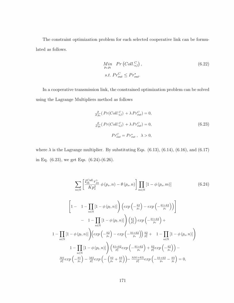
The constraint optimization problem for each selected cooperative link can be formu-

lated as follows.

Minps,pl

Pr(Coll.Cs,l

), (6.22)

s.t. PrCout ≤ Pr∗out.


using the Lagrange Multipliers method as follows

∂∂ ps

(Pr(Coll.Cs,l) + λPrCout) = 0,

∂∂ pl

(Pr(Coll.Cs,l) + λPrCout) = 0, (6.23)

PrCout = Pr∗out , λ > 0,

where λ is the Lagrange multiplier. By substituting Eqs. (6.13), (6.14), (6.16), and (6.17)

in Eq. (6.23), we get Eqs. (6.24)-(6.26).

∑n∈N

[IColl.th rγsnKp2

s


] ∏m∈N

[1− φ (ps,m)] (6.24)

[1−

(1−

∏n∈N

[1− φ (pl, n)]

)(exp

(−k2ps

)− exp

(−k1+k2

ps

))]

−

(1−

∏n∈N

[1− φ (pl, n)]

)(k1p2s

)exp

(−k1+k2

ps

)+(

1−∏n∈N

[1− φ (pl, n)]

)(exp

(−k2ps

)− exp

(−k1+k2

ps

))k2p2s

+

(1−

∏n∈N

[1− φ (ps, n)]

)(

1−∏n∈N

[1− φ (pl, n)]

)(k1+k2p2s

exp(−k1+k2

ps

)+ k2

p2sexp

(−k2ps

))−

λk1p2sexp

(−k1ps

)− λk2

p2sexp

(−(k2ps

+ k3pl

))− λ(k1+k2)

p2sexp

(−k1+k2

ps− k3

pl

)= 0,

171

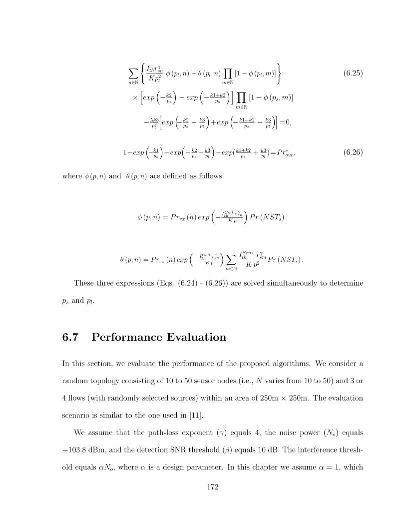
∑n∈N

Ithr

γsn

Kp2l


[1− φ (pl,m)]

(6.25)

×[exp

(−k2ps

)− exp

(−k1+k2

ps

)] ∏m∈N

[1− φ (ps,m)]

−λk3p2l

[exp

(−k2ps− k3

pl

)+exp

(−k1+k2

ps− k3

pl

)]=0,

1−exp(−k1ps

)−exp

(−k2ps− k3

pl

)−exp(k1+k2

ps+ k3

pl)=Pr∗out, (6.26)

where φ (p, n) and θ (p, n) are defined as follows


K p

)Pr (NSTs) ,


K p

)∑m∈N

ISens.th rγsmK p2

Pr (NSTs) .

These three expressions (Eqs. (6.24) - (6.26)) are solved simultaneously to determine

ps and pl.

6.7 Performance Evaluation

In this section, we evaluate the performance of the proposed algorithms. We consider a

random topology consisting of 10 to 50 sensor nodes (i.e., N varies from 10 to 50) and 3 or

4 flows (with randomly selected sources) within an area of 250m × 250m. The evaluation

scenario is similar to the one used in [11].

We assume that the path-loss exponent (γ) equals 4, the noise power (No) equals

−103.8 dBm, and the detection SNR threshold (β) equals 10 dB. The interference thresh-

old equals αNo, where α is a design parameter. In this chapter we assume α = 1, which

172

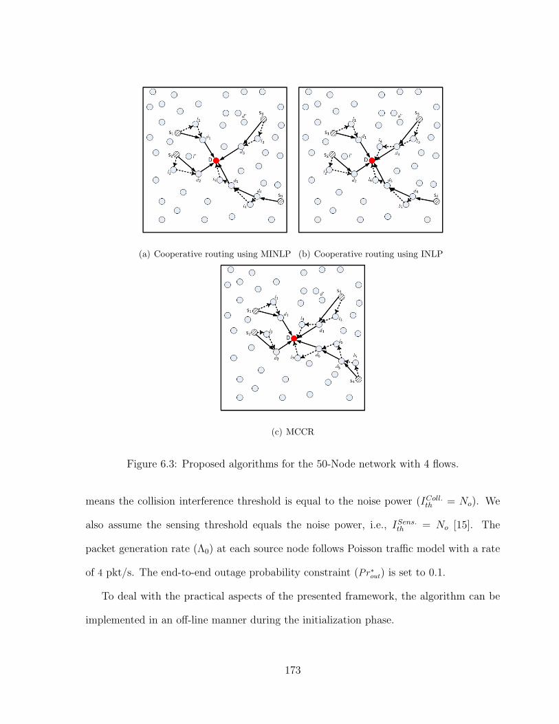
(a) Cooperative routing using MINLP (b) Cooperative routing using INLP

(c) MCCR

Figure 6.3: Proposed algorithms for the 50-Node network with 4 flows.

means the collision interference threshold is equal to the noise power (IColl.th = No). We

also assume the sensing threshold equals the noise power, i.e., ISens.th = No [15]. The

packet generation rate (Λ0) at each source node follows Poisson traffic model with a rate

of 4 pkt/s. The end-to-end outage probability constraint (Pr∗out) is set to 0.1.

To deal with the practical aspects of the presented framework, the algorithm can be

implemented in an off-line manner during the initialization phase.

173

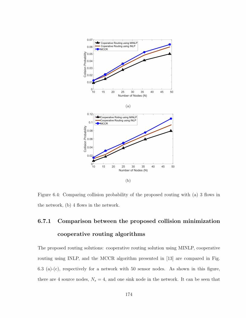
Number of Nodes (N)10 15 20 25 30 35 40 45 50

Col

isio

n Pr

obab

ility

0

0.01

0.02

0.03

0.04

0.05

0.06

0.07 Coperative Routing using MINLP Coperative Routing using INLPMCCR

(a)

Number of Nodes (N)10 15 20 25 30 35 40 45 50

Col

lisio

n Pr

obab

ility

0

0.02

0.04

0.06

0.08

0.1

0.12Cooperative Roting using MINLPCooperative Routing using INLPMCCR

(b)

Figure 6.4: Comparing collision probability of the proposed routing with (a) 3 flows in

the network, (b) 4 flows in the network.

6.7.1 Comparison between the proposed collision minimization

cooperative routing algorithms

The proposed routing solutions: cooperative routing solution using MINLP, cooperative

routing using INLP, and the MCCR algorithm presented in [13] are compared in Fig.

6.3 (a)-(c), respectively for a network with 50 sensor nodes. As shown in this figure,

there are 4 source nodes, Ns = 4, and one sink node in the network. It can be seen that

174

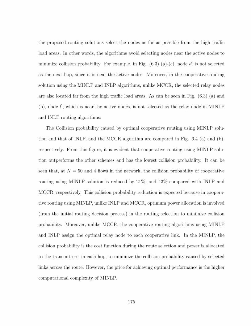
the proposed routing solutions select the nodes as far as possible from the high traffic

load areas. In other words, the algorithms avoid selecting nodes near the active nodes to

minimize collision probability. For example, in Fig. (6.3) (a)-(c), node d′

is not selected

as the next hop, since it is near the active nodes. Moreover, in the cooperative routing

solution using the MINLP and INLP algorithms, unlike MCCR, the selected relay nodes

are also located far from the high traffic load areas. As can be seen in Fig. (6.3) (a) and

(b), node l′, which is near the active nodes, is not selected as the relay node in MINLP

and INLP routing algorithms.

The Collision probability caused by optimal cooperative routing using MINLP solu-

tion and that of INLP, and the MCCR algorithm are compared in Fig. 6.4 (a) and (b),

respectively. From this figure, it is evident that cooperative routing using MINLP solu-

tion outperforms the other schemes and has the lowest collision probability. It can be

seen that, at N = 50 and 4 flows in the network, the collision probability of cooperative

routing using MINLP solution is reduced by 21%, and 43% compared with INLP and

MCCR, respectively. This collision probability reduction is expected because in coopera-

tive routing using MINLP, unlike INLP and MCCR, optimum power allocation is involved

(from the initial routing decision process) in the routing selection to minimize collision

probability. Moreover, unlike MCCR, the cooperative routing algorithms using MINLP

and INLP assign the optimal relay node to each cooperative link. In the MINLP, the

collision probability is the cost function during the route selection and power is allocated

to the transmitters, in each hop, to minimize the collision probability caused by selected

links across the route. However, the price for achieving optimal performance is the higher

computational complexity of MINLP.

175

6.7.2 Evaluating the effect of cooperative routing parameters

To investigate the effect of each of the cooperative routing parameters (cooperative path

selection, relay selection, and cooperative power allocation) separately in minimizing the

collision probability (i.e., one technique is used, while the other two are not employed), we

developed two additional routing algorithms. In the first one, called Cooperative Along

Minimum Collision Direct path (CAMCD), cooperation is employed after constructing the

route with the minimum collision probability using direct links only. Therefore, it does

not take into account the possibility of using cooperative links during route selection.

However, after route selection, it may use cooperative transmission over the links of

the selected route. The second algorithm, called Minimum Collision Non-cooperative

(MCN), considers only direct links during both the route selection and signal transmission.

CAMCD and MCN use optimal power allocation, as explained in Section 6.6.

As shown in the Fig. 6.5, taking into account the possibility of using cooperative

link during the route selection in cooperative routing using MINLP contributed 42% in

minimizing collision probability. Moreover, comparing the performance of cooperative

routing using MINLP and MCN to minimize collision reveals that cooperation trans-

mission contributes 57% in collision reduction of the cooperative routing using MINLP

algorithm.

Furthermore, in order to gain insight into the effect of the optimal power allocation

to minimize the caused collision probability with cooperative routing using MINLP, we

compare the performance of the algorithm with optimal power allocation with that of

the algorithm with equal power allocation (i.e., ps = pl = 0 dBm for all nodes in the

route). As shown in Fig. 6.5, the contribution of optimal power allocation in the collision

176

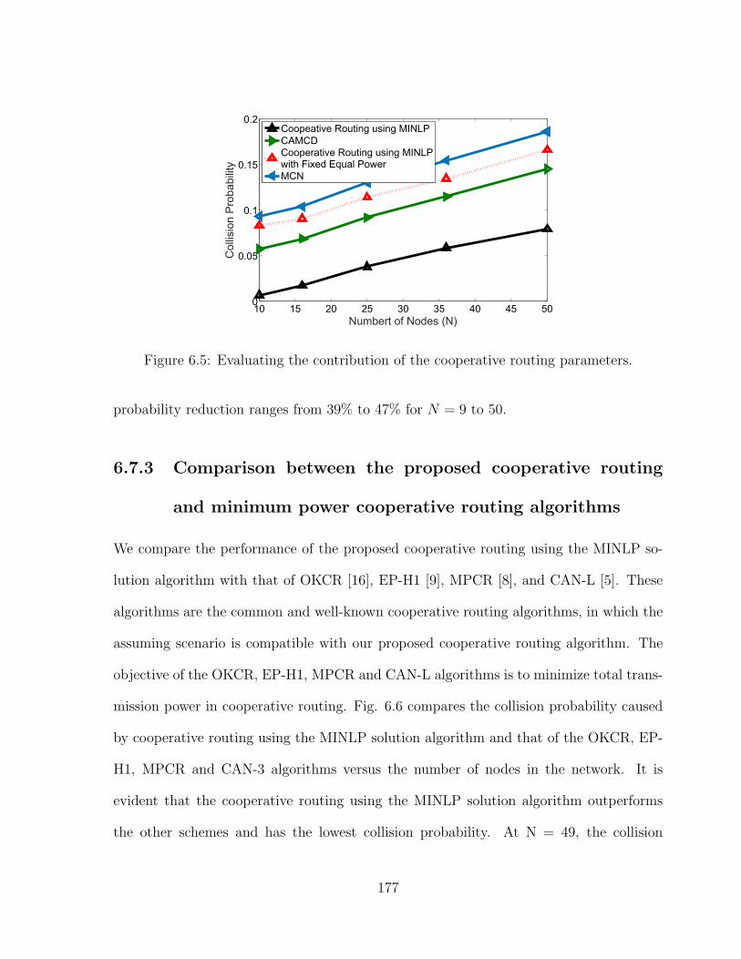
10 15 20 25 30 35 40 45 500

0.05

0.1

0.15

0.2

Numbert of Nodes (N)

Col

lisio

n Pr

obab

ility

Coopeative Routing using MINLPCAMCDCooperative Routing using MINLPwith Fixed Equal PowerMCN

Figure 6.5: Evaluating the contribution of the cooperative routing parameters.

probability reduction ranges from 39% to 47% for N = 9 to 50.

6.7.3 Comparison between the proposed cooperative routing

and minimum power cooperative routing algorithms

We compare the performance of the proposed cooperative routing using the MINLP so-

lution algorithm with that of OKCR [16], EP-H1 [9], MPCR [8], and CAN-L [5]. These

algorithms are the common and well-known cooperative routing algorithms, in which the

assuming scenario is compatible with our proposed cooperative routing algorithm. The

objective of the OKCR, EP-H1, MPCR and CAN-L algorithms is to minimize total trans-

mission power in cooperative routing. Fig. 6.6 compares the collision probability caused

by cooperative routing using the MINLP solution algorithm and that of the OKCR, EP-

H1, MPCR and CAN-3 algorithms versus the number of nodes in the network. It is

evident that the cooperative routing using the MINLP solution algorithm outperforms

the other schemes and has the lowest collision probability. At N = 49, the collision

177

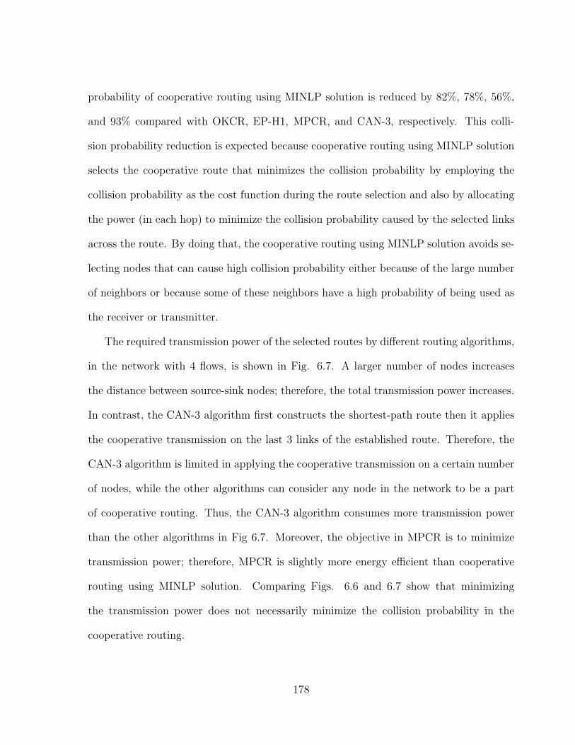
probability of cooperative routing using MINLP solution is reduced by 82%, 78%, 56%,

and 93% compared with OKCR, EP-H1, MPCR, and CAN-3, respectively. This colli-

sion probability reduction is expected because cooperative routing using MINLP solution

selects the cooperative route that minimizes the collision probability by employing the

collision probability as the cost function during the route selection and also by allocating

the power (in each hop) to minimize the collision probability caused by the selected links

across the route. By doing that, the cooperative routing using MINLP solution avoids se-

lecting nodes that can cause high collision probability either because of the large number

of neighbors or because some of these neighbors have a high probability of being used as

the receiver or transmitter.


in the network with 4 flows, is shown in Fig. 6.7. A larger number of nodes increases

the distance between source-sink nodes; therefore, the total transmission power increases.

In contrast, the CAN-3 algorithm first constructs the shortest-path route then it applies

the cooperative transmission on the last 3 links of the established route. Therefore, the

CAN-3 algorithm is limited in applying the cooperative transmission on a certain number

of nodes, while the other algorithms can consider any node in the network to be a part

of cooperative routing. Thus, the CAN-3 algorithm consumes more transmission power

than the other algorithms in Fig 6.7. Moreover, the objective in MPCR is to minimize

transmission power; therefore, MPCR is slightly more energy efficient than cooperative

routing using MINLP solution. Comparing Figs. 6.6 and 6.7 show that minimizing

the transmission power does not necessarily minimize the collision probability in the

cooperative routing.

178

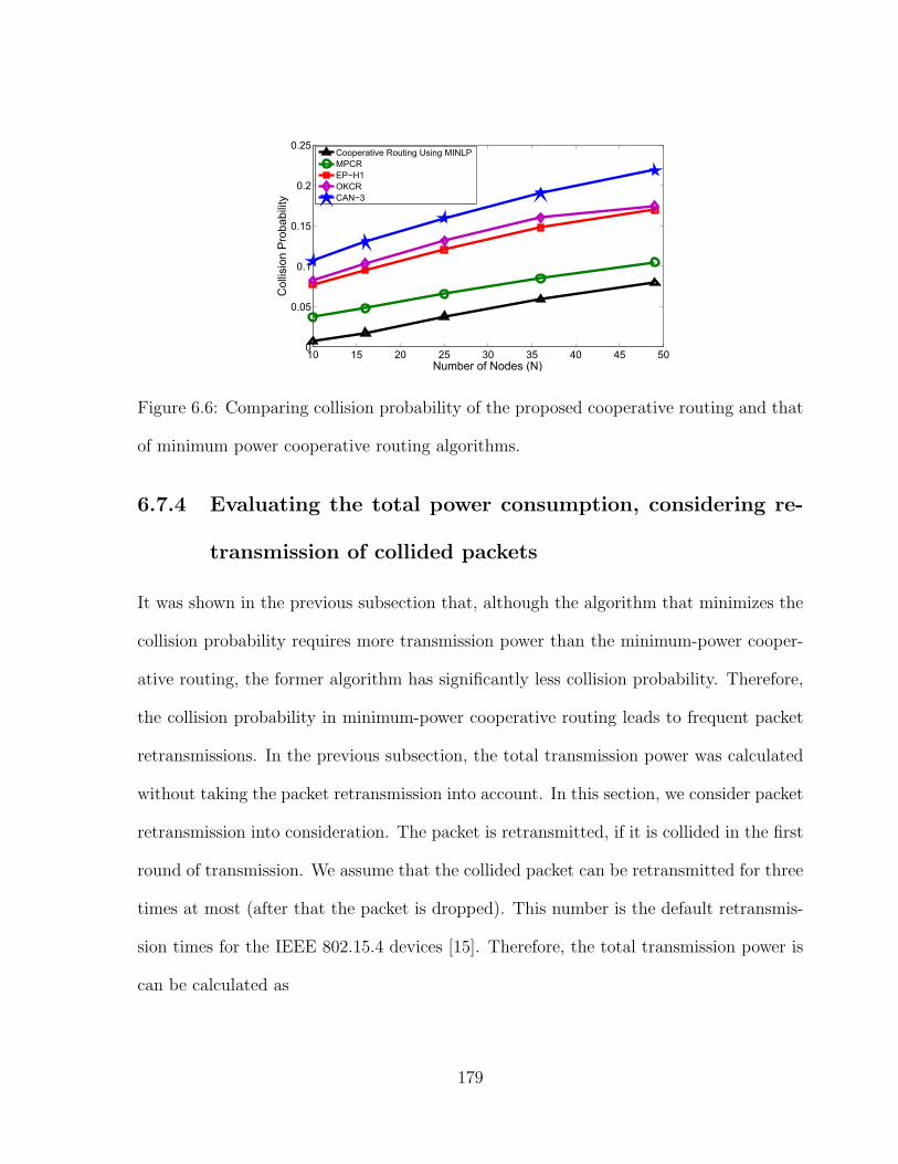
10 15 20 25 30 35 40 45 500

0.05

0.1

0.15

0.2

0.25

Number of Nodes (N)

Col

lisio

n Pr

obab

ility

Cooperative Routing Using MINLP MPCREP−H1OKCRCAN−3

Figure 6.6: Comparing collision probability of the proposed cooperative routing and that

of minimum power cooperative routing algorithms.

6.7.4 Evaluating the total power consumption, considering re-

transmission of collided packets

It was shown in the previous subsection that, although the algorithm that minimizes the

collision probability requires more transmission power than the minimum-power cooper-

ative routing, the former algorithm has significantly less collision probability. Therefore,

the collision probability in minimum-power cooperative routing leads to frequent packet

retransmissions. In the previous subsection, the total transmission power was calculated

without taking the packet retransmission into account. In this section, we consider packet

retransmission into consideration. The packet is retransmitted, if it is collided in the first

round of transmission. We assume that the collided packet can be retransmitted for three

times at most (after that the packet is dropped). This number is the default retransmis-

sion times for the IEEE 802.15.4 devices [15]. Therefore, the total transmission power is

can be calculated as

179

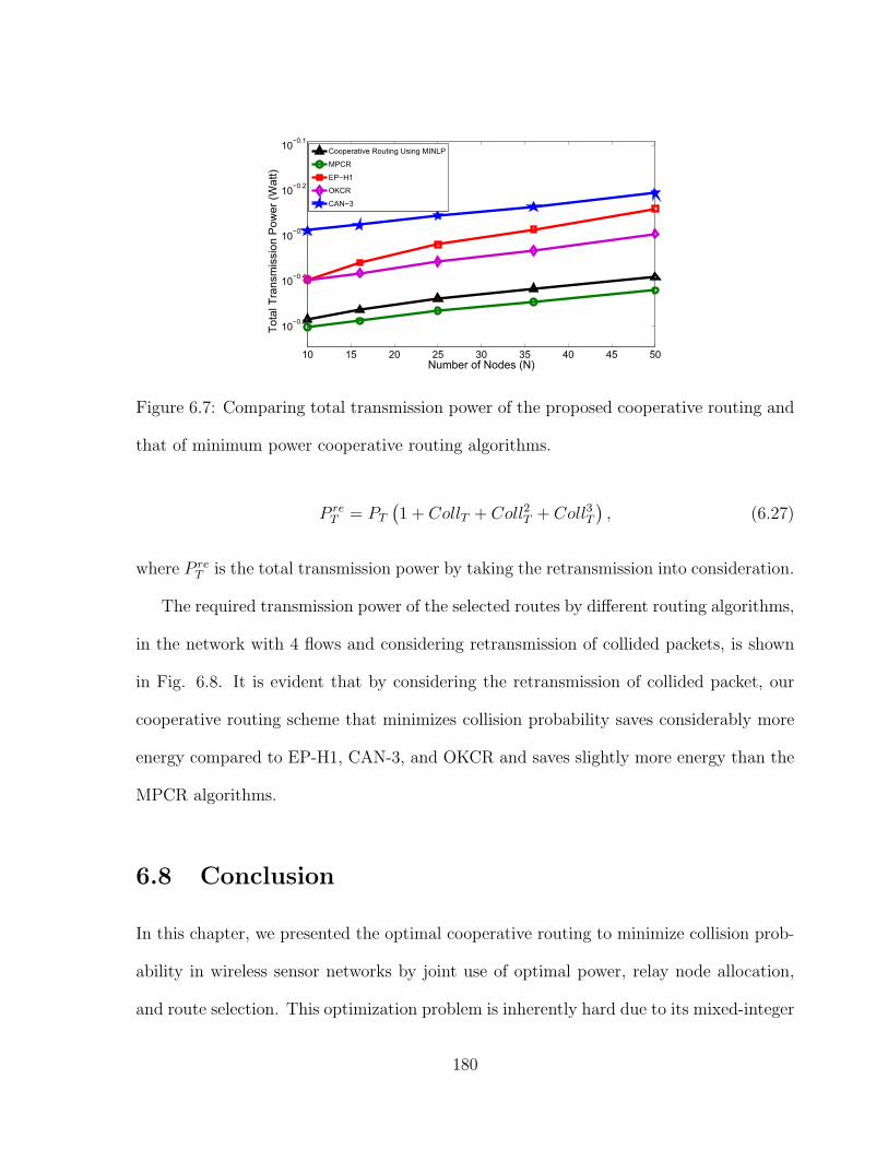
10 15 20 25 30 35 40 45 50

10−0.5

10−0.4

10−0.3

10−0.2

10−0.1

Number of Nodes (N)

Tota

l Tra

nsm

issi

on P

ower

(Wat

t)

Cooperative Routing Using MINLP

MPCR

EP−H1

OKCR

CAN−3

Figure 6.7: Comparing total transmission power of the proposed cooperative routing and

that of minimum power cooperative routing algorithms.

P reT = PT

(1 + CollT + Coll2T + Coll3T

), (6.27)

where P reT is the total transmission power by taking the retransmission into consideration.


in the network with 4 flows and considering retransmission of collided packets, is shown

in Fig. 6.8. It is evident that by considering the retransmission of collided packet, our

cooperative routing scheme that minimizes collision probability saves considerably more

energy compared to EP-H1, CAN-3, and OKCR and saves slightly more energy than the

MPCR algorithms.

6.8 Conclusion

In this chapter, we presented the optimal cooperative routing to minimize collision prob-

ability in wireless sensor networks by joint use of optimal power, relay node allocation,

and route selection. This optimization problem is inherently hard due to its mixed-integer

180

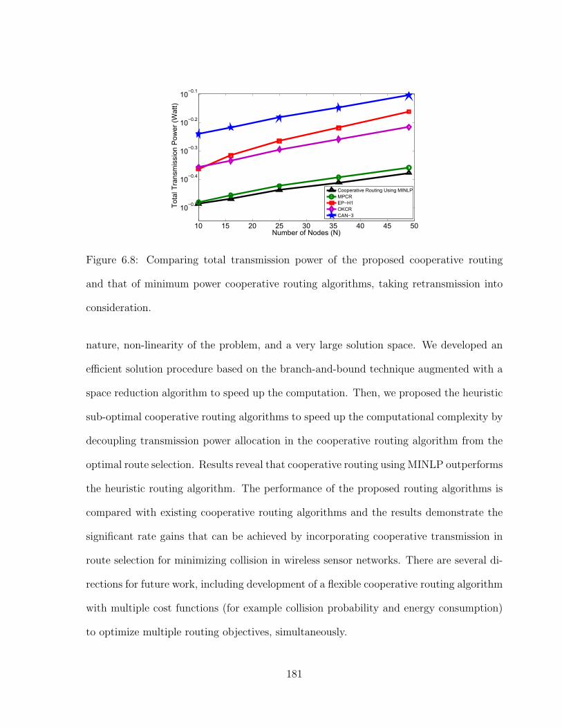
10 15 20 25 30 35 40 45 50

10−0.5

10−0.4

10−0.3

10−0.2

10−0.1

Number of Nodes (N)

Tota

l Tra

nsm

issi

on P

ower

(Wat

t)

Cooperative Routing Using MINLPMPCREP−H1OKCRCAN−3

Figure 6.8: Comparing total transmission power of the proposed cooperative routing

and that of minimum power cooperative routing algorithms, taking retransmission into

consideration.

nature, non-linearity of the problem, and a very large solution space. We developed an

efficient solution procedure based on the branch-and-bound technique augmented with a

space reduction algorithm to speed up the computation. Then, we proposed the heuristic

sub-optimal cooperative routing algorithms to speed up the computational complexity by

decoupling transmission power allocation in the cooperative routing algorithm from the

optimal route selection. Results reveal that cooperative routing using MINLP outperforms

the heuristic routing algorithm. The performance of the proposed routing algorithms is

compared with existing cooperative routing algorithms and the results demonstrate the

significant rate gains that can be achieved by incorporating cooperative transmission in

route selection for minimizing collision in wireless sensor networks. There are several di-

rections for future work, including development of a flexible cooperative routing algorithm

with multiple cost functions (for example collision probability and energy consumption)

to optimize multiple routing objectives, simultaneously.

181

Appendix

In [17], for a given source-destination pair with N nodes in the network, the number

of possible broadcasting trees from the source node to the destination node with zero

transmitters and zero relaying nodes (i.e., only the source node is transmitting the packet)

is given by

R (0) =

(N

N

)= 1, (6.28)

The number of possible broadcasting trees with one relay node is given by

R (1) =

(N

1

)N−1∑i=1

(N − 1

i

), (6.29)

the above formula means that we first need to pick one node as the relay node and then

decide how many nodes are reached directly by the relay node (the remaining nodes are

directly reached by the source node). The case of possible broadcasting trees with two

relay nodes is more complicated and is given by

R (2) =

(N

2

)N−2∑i=1

((N − 1

i

)N−2∑j=1

(N − 1− i

j

)). (6.30)

Therefore, the number of possible broadcasting trees with i relay nodes is given by

R (i) = (6.31)(N

i

) N−i∑k1=1

((N − 1

k1

) N−1∑k2=1

((N − 1− k1

k2

)

...

N−i∑kj=1

((N − 1−i−1∑j=1

kj

ki

)))...

).

The above formula means that we first need to pick i nodes as the relay nodes with a

number of possibilities of ((Ni

)) and then decide how many nodes are reached directly by

182

the relay node (the remaining nodes are directly reached by the source node). Therefore,

the total number of possible broadcasting trees in the network is given by

T =N−1∑i=0

R (i) . (6.32)

For example, for N = 15 (15 nodes in the network), the number of broadcasting trees

is more than 8.7 billion [17]. Since cooperative paths are mapped as broadcasting trees,

for the network with Ns there are NsT possible cooperative paths from the source nodes

to the destination node. Therefore, selecting the best path out of all possible paths is

NP-hard

REFERENCES



pp. 3062–3080, Dec. 2004.

[2] R. Madan, N. Mehta, A. Molisch, and J. Zhang, “Energy-efficient decentralized co-

operative routing in wireless networks,” IEEE Trans. Autom. Control, vol. 54, no. 3,

pp. 512–527, Mar. 2009.

[3] W. Zhuang and M. Ismail, “Cooperation in wireless communication networks,” IEEE

Trans. Wireless Commun., vol. 19, no. 2, pp. 10–20, Apr. 2012.

183

[4] A. Nosratinia, T. Hunter, and A. Hedayat, “Cooperative communication in wireless

networks,” IEEE Commun. Mag., vol. 42, no. 10, pp. 74–80, Oct. 2004.

[5] A. E. Khandani, J. Abounadi, E. Modiano, and L. Zheng, “Cooperative routing

in static wireless networks,” IEEE Trans. Wireless Commun., vol. 55, no. 11, pp.

2185–2192, Nov. 2007.

[6] F. Mansourkiaie and M. Ahmed, “Cooperative routing in wireless networks: A com-

prehensive survey,” IEEE Commun. Surveys Tuts., vol. PP, no. 99, pp. 1–1, 2015.

[7] C. Pandana, W. Siriwongpairat, T. Himsoon, and K. Liu, “Distributed cooperative

routing algorithms for maximizing network lifetime,” in Proc. IEEE Wireless Com-

munications and Networking Conference, (WCNC), Apr. 2006, pp. 451–456.



Oct. 2008.



no. 11, pp. 3813–3823, Nov. 2011.

[10] J. Zhang and Q. Zhang, “Contention-aware cooperative routing in wireless mesh

networks,” in Proc. IEEE International Conference on Communications (ICC), June

2009, pp. 1–5.

[11] ——, “Cooperative routing in multi-source multi-destination multi-hop wireless net-

works,” in Proc. IEEE INFOCOM, Apr. 2008, pp. 306–310.

184

[12] B. Han, J. Li, J. Su, and J. Cao, “Self-supported cooperative networking for emer-

gency services in multi-hop wireless networks,” IEEE J. Sel. Areas Commun., vol. 30,

no. 2, pp. 450–457, Feb. 2012.

[13] F. Mansourkiaie and M. Ahmed, “Joint cooperative routing and power allocation

for collision minimization in wireless sensor networks with multiple flows,” IEEE

Wireless Communications Letters, vol. 4, no. 1, pp. 6–9, Feb 2015.

[14] J. Habibi, A. Ghrayeb, and A. Aghdam, “Energy-efficient cooperative routing in

wireless sensor networks: A mixed-integer optimization framework and explicit solu-

tion,” IEEE Trans. Commun., vol. 61, no. 8, pp. 3424–3437, Aug. 2013.



[16] P. Ahmadi and B. Jabbari, “An outage-aware power saving cooperative routing al-

gorithm in wireless networks,” in Wireless Telecom. Symp. (WTS), 2013, Apr. 2013,

pp. 1–5.

[17] F. Li and I. Nikolaidis, “On minimum-energy broadcasting in all-wireless networks,”

in Proc. IEEE 26th Conference on Local Computer Networks, (LCN), Nov. 2001, pp.

193–202.

185

Chapter 7

Conclusions and Future Work

7.1 Introduction

Cooperative routing is a cross-layer design approach that combines the network layer

and the physical layer to transmit packets through cooperative links. The goal of this

dissertation is to minimize collision probability subject to the outage probability con-

straint, employing optimal cooperative routing, power allocation and relay selection. In

this chapter, we summarize the contributions presented in this dissertation, draw main

conclusions, and discuss several potential extensions to our work.

7.2 Conclusions

The following conclusions can be drawn from this dissertation:

We started with a basic mathematical model for collision probability, in which the

probability of being in receiving mode for each node is obtained assuming the Poisson

186

arrival process. Then, we proposed a sub-optimal cooperative routing algorithm to

minimize collision probability in WSNs. The results revealed that, at N = 49, the

collision probability of the proposed cooperative routing algorithm using the Poisson

arrival traffic is reduced by 85%, 48%, and 70% compared with EP-H1 [1], MPCR

[2], and CAN-3 [3], respectively. Moreover, the results revealed that taking into

account the possibility of using cooperative links during the route selection in the

proposed sub-optimal cooperative routing algorithm, which used the Poisson arrival

traffic, contributed 40% in minimizing collision probability. Moreover, comparing

the performance of the proposed algorithm and that of the MCN algorithm revealed

that cooperation transmission (employing relay node for transmission) contributes

54% in collision reduction of the proposed cooperative routing algorithm.

We mathematically formulated the per-node traffic load in a cooperative link. The

traffic load of each node includes the traffic generated by the node itself and the

traffic generated by other nodes, which is forwarded by the node either as a next

hop of the route or as a relay node. We verified the accuracy of the proposed

mathematical model for the per-node traffic load using the simulation results. We

illustrated that there is a close match between analytical and simulation results.

Therefore, the proposed mathematical formula can accurately model the traffic load

of each node in cooperative routing. The results also confirmed that traffic load

increases as a function of the node’s vicinity to the sink node.

We employed the proposed model of per-node traffic load to obtain the mathemat-

ical model for collision probability of direct and cooperative transmission. For a

cooperative transmission, we started with a simple cooperative transmission link,

187

where each link consists of a source, destination, and a potential relay node. For

this three-node cooperative transmission model, we mathematically analysed the

collision probability caused by a cooperative link to all nodes in the network.

We developed an optimization framework to obtain the cooperative route that causes

minimum collision to other nodes of the network. The problem was formulated as

the mixed integer non-linear programming problem. The complexity of the problem

is discussed and we proved that the minimum collision cooperative routing problem

is NP-Hard.

To solve MINLP, we enhanced the BnB technique and developed the space reduc-

tion BnB algorithm which reduced the searching space of the branch and bound

algorithm and increased the speed of convergence in BnB. The algorithm applied a

joint optimization approach for power allocation, relay node assignment, and path

selection which are the main optimization issues in cooperative routing. By doing

that, the cooperative routing using MINLP solution avoids selecting nodes that can

cause high collision probability either because of the large number of neighbors or

because some of these neighbors have a high probability of being used as the receiver

or transmitter.

Due to the computational complexity of solving MINLP, two near-optimal heuris-

tic cooperative routing algorithms were proposed by decoupling the optimization

variables. In the first near-optimal cooperative routing, namely, cooperative rout-

ing using INLP, optimal power was allocated after route selection and relay node

assignment. Therefore, optimal cooperative routing selection and rely node assign-

ment were deployed in the first phase and the optimal power was allocated in the

188

second phase. In the second near-optimal cooperative routing, namely, Minimum

Collision Cooperative Routing (MCCR), firstly, the optimal cooperative routing

selected and secondly, optimal power allocated and relay node assigned.

We illustrated that the MINLP solution serves as the benchmark and we evaluated

the quality of the solution obtained by any sub-optimal algorithm of this problem.

The simulation results revealed that cooperative routing using MINLP outperforms

the near-optimal heuristic routing algorithms. We illustrated that for a network

with 50 sensor nodes including 4 source nodes, the collision probability cased by

the routing using MINLP was reduced by 21% and 43% compared with INLP and

MCCR, respectively. However, the price of achieving optimal performance in coop-

erative routing using MINLP is the higher computational complexity.

We illustrated that the computational complexity of cooperative routing using

MINLP and INLP grow exponentially with the number of nodes versus the polyno-

mial complexity of the MCCR algorithm.

We developed two additional routing algorithms to investigate the effects of each

cooperative routing optimization variables in minimizing the collision probability

of cooperative routing using MINLP. The simulation results, for a network with 50

nodes and 4 source nodes, revealed that taking into account the possibility of us-

ing cooperative link during the route selection in cooperative routing using MINLP

contributed 42% in minimizing collision probability. Moreover, cooperation trans-

mission (employing relay node for transmission) contributed 57% in collision reduc-

tion of the cooperative routing using MINLP algorithm. Furthermore, in order to

gain insight into the effect of the optimal power allocation to minimize the caused

189

collision probability with cooperative routing using MINLP, we compared the per-

formance of the algorithm with optimal power allocation with that of the algorithm

with equal power allocation. The results reveal that the contribution of optimal

power allocation in the collision probability reduction ranges from 39% to 47% for

a network with 9 to 50 nodes.

We compare the performance of the proposed cooperative routing using the MINLP

solution algorithm with that of EP-H1, MPCR, and CAN-3, where the objective of

the algorithms is to minimize total transmission power in cooperative routing. We

illustrated that the cooperative routing using the MINLP solution algorithm out-

performs the other schemes and has the lowest collision probability. For a network

with 50 nodes in the network including 4 source nodes, the collision probability

of cooperative routing using MINLP solution is reduced by 93%, 56%, and 78%

compared with EP-H1, MPCR, and CAN-3, respectively.

We illustrated that the MPCR algorithm is slightly more energy efficient than the

cooperative routing using the MINLP solution. Comparing collision probability as

well as the required transmission power of the proposed algorithm with the existing

energy efficient cooperative routing algorithms, such as MPCR, EP-H1, and CAN-3,

proved that minimizing the transmission power does not necessarily minimize the

collision probability in the cooperative routing.

190

7.3 Future Work

In Chapter 2 of this dissertation, we have presented a comprehensive review of existing co-

operative routing protocols. The main challenges associated with optimal route selection

and the design requirements of cooperative routing protocols are discussed to provide an

insight into the objectives of routing protocols. An accurate classification of the protocols

is given and the merits and disadvantages of the protocols are determined. Despite the

large number of research activities and the rapid and significant progress that being made

in cooperative routing in recent years, numerous avenues for further research remain. The

following research issues are outlined for future investigation:

Multiple Objectives: While offering a single objective supports one goal, routing

algorithms should be flexible to support various application-specific requirements,

such as throughput, capacity, coverage, end-to-end delay, real-time delay, and col-

lision. So, designing flexible cooperative routing protocols with multiple cost func-

tions to optimize multiple objectives can be reckoned as an interesting area for

future research.

Multi-constrained QoS guarantee: Cooperative routing algorithms should be flexi-

ble enough to support different application-specific QoS requirements, such as out-

age probability, end-to-end delay, delay jitter, and bandwidth consumption. Thus

far, outage probability has been the main QoS requirement considered in coopera-

tive routing algorithms. Although diverse QoS constraints need to be considered,

satisfying some QoS metrics in certain wireless networks is in contradiction with

achieving other constraints or objectives. For instance, in vehicular ad hoc net-

works, satisfying QoS is in contradiction with achieving more energy efficiency [4].

191

Therefore, designing a flexible cooperative routing with adaptive cost functions to

provide multi-constrained QoS guarantee is viewed as an interesting area for future

investigation.

Nodes Mobility: Almost in all proposed cooperative routing algorithms, the nodes

are assumed to be static. Recently, there has been an increased interest in appli-

cations that support the mobility of users, such as cellular networks and Vehicular

Ad Hoc Networks (VANET). An example for this application is the medical-care

application, where the mobile wireless network nodes are attached to the patients

and need to send continuous data from the patient to the doctor. There is only

one cooperative routing protocol that covers mobility (i.e., [5]) and there is much

potential for future research in this area. On the other hand, mobility can pose some

challenges in cooperative protocol design, such as dynamic relay node assignment

methods.

Security: It has been shown in the literature that the appropriate design of cooper-

ative routing can extend the coverage and improve the performance of the network.

However, the security issues raised by increasing the network coverage and allow-

ing nodes to manipulate the signals of other nodes at the signal level (e.g., signal

detection by the DF relays and signal combining at each receiving node) are not

well-studied. Secure routing is an issue that needs further attention. Moreover,

although security was not an objective in the design of recent cooperative routing

algorithms, it is important to analyze the performance of these algorithms when

security concerns are incorporated.

Energy Harvesting (EH): Energy is harvested using solar, vibration, and other phys-

192

ical phenomena [6]. EH nodes harvest energy from the environment to carry out

their communication tasks. Use of energy harvesting nodes as the relay nodes in

cooperative diversity is proved to be a promising and emerging solution in energy-

limited wireless networks [7,8]. However, none of the proposed cooperative routing

algorithms are energy harvesting aware.

Applications: Although there has been extensive work on employing cooperative

routing in WSNs, there have been very few works that consider cooperative routing

in other network applications, such as delay-sensitive applications and bandwidth-

limited applications. Therefore, potential applications of cooperative routing, such

as cognitive radio networks, LTE networks, wireless LANs, and cellular networks

are an interesting area for future investigation.

Implementations: Most of the cooperative routing algorithms surveyed in this paper

have been evaluated through theoretical analysis and simulation; only one proposed

algorithm, namely EERWSN [9], deals with the practical aspects of cooperative

routing. The authors in [9] used parametric programming in an off-line manner to

reduce the computational requirements for the sensor nodes to very simple opera-

tions during network functioning. Further investigation and improvements to the

current implementation approaches are identified as an area for future work.

193

REFERENCES



no. 11, pp. 3813–3823, 2011.



Oct. 2008.

[3] A. Khandani, J. Abounadi, E. Modiano, and L. Zheng, “Cooperative routing in static

wireless networks,” IEEE Trans. Commun., vol. 55, no. 11, pp. 2185–2192, Nov. 2007.

[4] Z. Sheng, Z. Ding, and K. Leung, “Distributed and power efficient routing in wireless

cooperative networks,” in Proc. IEEE International Conference on Communications

(ICC), June 2009, pp. 1–5.

[5] W.-H. Chen, A.-C. Pang, A.-C. Pang, and C.-T. F. Chiang, “Cross-layer cooperative

routing for vehicular networks,” in Proc. IEEE International Computer Symposium

(ICS), Dec. 2010, pp. 67–72.

[6] J. Paradiso and T. Starner, “Energy scavenging for mobile and wireless electronics,”

IEEE Pervasive Comput., vol. 4, no. 1, pp. 18–27, Jan 2005.

194

[7] B. Medepally and N. Mehta, “Voluntary energy harvesting relays and selection in

cooperative wireless networks,” Wireless Communications, IEEE Transactions on,

vol. 9, no. 11, pp. 3543–3553, November 2010.

[8] L. Liu, R. Zhang, and K.-C. Chua, “Wireless information transfer with opportunistic

energy harvesting,” IEEE Transactions on Wireless Communications, vol. 12, no. 1,

pp. 288–300, January 2013.

[9] J. Habibi, A. Ghrayeb, and A. Aghdam, “Energy-efficient cooperative routing in wire-

less sensor networks: A mixed-integer optimization framework and explicit solution,”

IEEE Trans. Commun., vol. 61, no. 8, pp. 3424–3437, Aug. 2013.

195

cooperative routing for collision minimization in wireless

Documents