control improvisation with probabilistic temporal specifications
TRANSCRIPT

Control Improvisation with Probabilistic Temporal Specifications
Ilge Akkaya, Daniel J. Fremont, Rafael Valle,Alexandre Donze, Edward A. Lee, and Sanjit A. Seshia
Abstract— We consider the problem of generating random-ized control sequences for complex networked systems typi-cally actuated by human agents. Our approach leverages aconcept known as control improvisation, which is based on acombination of data-driven learning and controller synthesisfrom formal specifications. We learn from existing data agenerative model (for instance, an explicit-duration hiddenMarkov model, or EDHMM) and then supervise this model inorder to guarantee that the generated sequences satisfy somedesirable specifications given in Probabilistic Computation TreeLogic (PCTL). We present an implementation of our approachand apply it to the problem of mimicking the use of lightingappliances in a residential unit, with potential applications tohome security and resource management. We present exper-imental results showing that our approach produces realisticcontrol sequences, similar to recorded data based on humanactuation, while satisfying suitable formal requirements.
I. INTRODUCTION
The promise of the emerging Internet of Things (IoT) is toleverage the programmability of connected devices to enableapplications such as connected smart vehicles, occupancy-based automated HVAC control, autonomous robotic surveil-lance, and much more. However, this promise cannot be real-ized without better tools for the automated programming andcontrol of a network of devices — computational platforms,sensors, and actuators. Traditionally, this problem has beenapproached from two different angles. The first approachis to be data-driven, leveraging the ability of devices andsensors to collect vast amounts of data about their operationand environments, and using learning algorithms to adjust theworking of these devices to optimize desired objectives. Thisapproach, exemplified by devices such as smart learning ther-mostats, can be very effective in many settings, but typicallycannot give any guarantees of correct operation. The secondapproach is to be model-driven, where accurate models of thedevices and their operating environment are used to definea suitable control problem. A controller is then synthesizedto guarantee correct operation under specified environmentconditions. However, such an approach is difficult in settingswhere such accurate models are hard to come by. Moreover,strong correctness guarantees may not be needed in all cases.
This work was supported in part by TerraSwarm, one of six centers ofSTARnet, a Semiconductor Research Corporation program sponsored byMARCO and DARPA.
All authors are with the Department of Electrical En-gineering and Computer Science, UC Berkeley, Berkeley,CA 94720, USA [email protected],[email protected], [email protected],[email protected], [email protected],[email protected]
Consider, for instance, the application domain of homeautomation. More specifically, consider a scenario where oneis designing the controller for a home security system thatcontrols the lighting (and possibly other appliances) in ahome when the occupants are away. One might want toprogram the system to mimic typical human behavior interms of turning lights on and off. As human behavior issomewhat random, varying day to day, one might want thecontroller to exhibit random behavior. However, completelyrandom control may be undesirable, since the system mustobey certain time-of-day behavioral patterns, and respectcorrelations between devices. For these requirements, a data-driven approach where one learns a randomized controllermimicking human behavior seems like a good fit. It isimportant to note, though, that such an application may alsohave constraints for which provable guarantees are needed,such as limits on energy consumption being obeyed withhigh probability, or that multiple appliances never be turnedon simultaneously. A model-based approach is desirablefor these. Thus, the overall need is to blend data andmodels to synthesize a control strategy that obeys certainhard constraints (that must always be satisfied), certain softconstraints (that must be “mostly satisfied”) and certainrandomness requirements on system behavior.
This setting has important differences from typical controlproblems. For example, in traditional supervisory control, thegoal is typically to synthesize a control strategy ensuring thatcertain mathematically-specified (formal) requirements holdon the entity being controlled (the “plant”). Moreover, thegenerated sequence of control inputs is typically completelydetermined by the state of the plant. Predictability andcorrectness guarantees are important concerns. In contrast, inthe home automation application sketched above, predictabil-ity is not that important. Indeed, the system’s behaviormust be random, within constraints. Moreover, the sourceof randomness (behavior of human occupants) differs fromhome to home, and so this cannot be pre-programmed.
This form of randomized control is suitable for human-in-the-loop systems or applications where randomness is desir-able for reasons of security, privacy, or diversity. Applicationdomains other than the home automation setting describedabove include microgrid scheduling [14], [7] and robotic art[3]. In the former, randomness can provide some diversityof load behavior, hence making the grid more efficient interms of peak power shaving and more resilient to correlatedfaults or attacks on deterministic behavior. For the latter case,there is growing interest in augmenting human performanceswith computational aids, such as in automatic synthesis and
arX
iv:1
511.
0227
9v1
[cs
.SY
] 7
Nov
201
5

improvisation of music [5]. All these applications sharethe property of requiring some randomness while main-taining behavior within specified constraints. Additionally,the human-in-the-loop applications can benefit from data-driven methods. Streams of time-stamped data from devicescan be used to learn semantic models capturing behavioralcorrelations amongst them for further use in programmingand control.
In this paper, we show how a recently-proposed formalismtermed control improvisation [6] can be suitably adapted toaddress the problem of randomized control for IoT systems.We consider the specific setting of a system whose compo-nents can be controlled either by humans or automatically.Human control of devices generates data comprising streamsof time-stamped events. From such data, we show howone can learn a nominal randomized controller respectingcertain constraints present in the data including correlationsbetween behavior of interacting components. We also showhow additional constraints can be enforced on the outputof the controller using temporal logic specifications andverification methods based on model checking [4], [11]. Weapply our approach to the problem of randomized controlof home appliances described above. We present simulatedexperimental results for the problem of lighting control basedon data from the UK Domestic Appliance-Level Electricity(UK-DALE) dataset [10]. Our approach produces realisticcontrol sequences, similar to recorded data based on humanactuation, while also satisfying suitable formal requirements.
The rest of the paper is organized as follows: in Section II,we give some preliminary background on the formalismsused throughout the paper. We formally define our problemas an instance of control improvisation, and describe ourtechnique for solving it, in Section III. Next, Section IVpresents detailed experimental results from a case study onlighting improvisation. Finally, we conclude the paper withrelated work and future directions in Sections V and VIrespectively.
II. BACKGROUND
We introduce relevant background material that the presentpaper builds upon and establish notation for use in the restof the paper.
A. Discrete-Event Systems with Hidden States
Our work focuses on control of systems whose behaviorcan be described by a sequence of timestamped events. Anevent e is a tuple 〈τ, v〉 ∈ T×V , where T is a totally orderedset of time stamps and V is a finite set of values. We definea signal to be a set of events, where T imposes an orderingrelation on the events occurring within the signal [12].
We define the state of such a system to take values from afinite set of distinct states, where events are emitted by statetransitions. In many systems, the underlying events and statesare hidden, and all that can be observed is some function ofthe state. We term this the observation. This function can betime-dependent and probabilistic, so that a single state canproduce many different observations. We assume that the
hour of day
19 20 21 22 23
InstantaneousApplian
cePow
er(W
)
0
50
100
150
200
250
kitchenliving roombedroomkitchen ONkitchen OFFliving room ONliving room OFFbedroom ONbedroom OFF
Fig. 1: Sample appliance power trace
number of possible observation values is finite (this can beenforced in continuous systems by discretization), and thatobservations are made at discrete time steps. A sequence ofobservations over time generated by a behavior of the systemis called a trace.
An example of such a trace that captures the powerconsumption of three appliances is given in Figure 1. Theevents related to each appliance, which can either be an “ON”or an “OFF” event in this case, are annotated on the sub-traces. Each state change of the system triggers an event.Consider, for example, that the hidden state in this scenariocaptures the current status of a set of physical appliancesand that all appliances are initially turned off. The kitchenappliance being turned on at 19:50 pm causes an “ON” eventto be emitted, and triggers a state change in the system,where in the new state, the kitchen appliance is on, andthe other two appliances are off. The system stays in thisstate until any appliance triggers a state transition. In sucha scenario, it may be that the only information that can beobserved from the system are traces of the instantaneouspower consumptions of the appliances. Given these traces,one can infer the state of the system and which events mayhave happened at particular times.
B. Control Improvisation
The control improvisation problem, defined formallyin [6], can be seen as the problem of generating a random se-quence of control actions subject to hard and soft constraints,while satisfying a randomness requirement. The hard con-straints may, for example, encode safety requirements on thesystem that must always be obeyed. The soft constraints canencode requirements that may occasionally be violated. Therandomness requirement ensures that no control sequenceoccurs with too high probability.
This problem is a natural fit to the applications of in-terest in this paper, as our end goal is to randomize thecontrol of discrete-event systems subject to both constraintsenforcing the presence of certain learned behaviors (hardconstraints), and probabilistic requirements upper boundingthe observations (soft constraints). In the lighting controlscenario we consider later, for example, we effectively learna hard constraint preventing multiple appliances from beingtoggled at exactly the same time, since this never occursin the training data. We also use soft constraints to limitthe probability that the hourly power consumption exceedsdesired bounds.

More formally, the control improvisation problem is de-fined as follows. This is generalized from the definition in [6]to allow soft constraints with different probabilities.
Definition 1: An instance of the control improvisation(CI) problem is composed of (i) a language I of improvi-sations that are strings over a finite alphabet Σ, i.e., I ⊆ Σ∗,and (ii) finitely many subsets Ai ⊆ I for i ∈ 1, . . . , n.These sets can be presented, for example, as finite automata,but for our purposes in this paper the details are unimportant(see [6] for a thorough discussion).
Given error probability bounds ε = (ε1, . . . , εn) withεi ∈ [0, 1], and a probability bound ρ ∈ (0, 1], a distributionD : Σ∗ → [0, 1] with support set S is an (ε, ρ)-improvisingdistribution if
(a) S ⊆ I (hard constraints),(b) ∀w ∈ S, D(w) ≤ ρ (randomness),(c) ∀i, P [w ∈ Ai | w ← D] ≥ 1− εi (soft constraints),
where w ← D indicates that w is drawn from the distributionD. An (ε, ρ)-improviser, or simply an improviser, is a proba-bilistic algorithm generating strings in Σ∗ whose output dis-tribution is an (ε, ρ)-improvising distribution. For example,this algorithm could be a Markov chain generating randomstrings in Σ∗. The control improvisation problem is, giventhe tuple (I, Ai, ε, ρ), to generate such an improviser.
C. Explicit-Duration Hidden Markov Models
d0
x0
d1
x1
y1
dt
xt
yt
dt+1
xt+1
yt+1
... ...d
T
xT
yT
Fig. 2: Graphical model representation of an EDHMM.
In data-driven controller synthesis, it is essential that thelearning model captures relevant properties of the underlyingdata. In applications where the data exhibits an underlyingbut hidden state space, and observations can be assumed tobe drawn from densities depending only on the current state,a Hidden Markov Model (HMM) is a good fit.
However, in many applications, including those of interestto this paper, the Markov assumption on the hidden statespace is insufficient, since part of the underlying structurelies in the durations of hidden events. In such scenarios,the model quality can be improved significantly by theuse of semi-Markov models. In this study, we will specif-ically consider the Explicit-Duration Hidden Markov Model(EDHMM) [13]. These models are an extension of hiddenMarkov models that, in addition to modeling the hidden statespace as a Markov chain, also introduces the duration spentwithin each state as another hidden variable of the Bayesiannetwork. The graphical model representation of a generalEDHMM is shown in Figure 2.
The standard definition of an EDHMM models hiddenstate and its duration to be discrete hidden variables. Thestate dependent observations can be drawn from either adiscrete or continuous distribution, often referred to as anemission distribution. In this paper, we assume that thepossible observations are quantized as necessary so that theemission distributions are discrete.
An EDHMM with discrete emissions observed for T timesteps is characterized by a partially observed set of variables(x,d,y) = (x1, . . . , xT , d1, . . . , dT , y1, . . . , yT ). Each xiindicates the hidden state of the model at time i, from afinite state space X which for notational convenience weassume to be the set 1, . . . , N. The value di ∈ 1, . . . , Ddenotes the remaining duration of the hidden state, where Dis the maximum possible duration. Finally, each yi is an ob-servation drawn from a discrete alphabet Σ = v1, . . . , vM.The joint probability distribution imposed by the EDHMMover these variables can be written as
P (x,d,y) = p(x1)p(d1)T∏t=2
p(xt|xt−1, dt−1)p(dt|dt−1, xt)T∏t=1
p(yt|xt)
= πxπd
T∏t=2
p(xt|xt−1, dt−1)p(dt|dt−1, xt)T∏t=1
p(yt|xt),
where p(x1) , πx and p(d1) , πd are the priors onthe hidden state and duration distributions, respectively. Theconditional state and duration dynamics are given by
p(xt|xt−1, dt−1) ,
p(xt|xt−1), dt−1 = 1
δ(xt, xt−1), otherwise(1)
p(dt|dt−1, xt) ,
p(dt|xt), if dt−1 = 1
δ(dt, dt−1 − 1), otherwise, (2)
where δ(·, ·) is the Kronecker delta function. Equations(1) and (2) specify the current state xt and the remainingduration dt for that state as a function of the previous stateand its remaining duration. Unless the remaining durationat the previous state is equal to 1, the state will remainunchanged across time steps, while at each step within thestate, the remaining duration is decremented by 1. Whenthe remaining duration is 1, the next state is sampled froma transition probability distribution p(xt|xt−1), while theremaining duration at xt is sampled from a state-dependentduration distribution p(dt|xt). All self-transition probabilitiesare set to zero: p(xt|xt−1) = 0 if xt = xt−1. For com-pactness of notation, for all xt, xt−1 ∈ 1, . . . , N, dt ∈1, . . . , D, and yt ∈ v1, . . . , vM we define probabilitiesaxt−1,xt , bxt,yt , and cxt,dt so that
p(xt|xt−1) =
axt−1,xt
, if xt 6= xt−1
0, otherwise,
p(yt|xt) = bxt,yt ,
p(dt|xt) = cxt,dt .
We consolidate these probabilities into an N × N statetransition matrix A , (aij), an N ×M emission probability

matrix B , (bij), and an N ×D duration probability matrixC , (cij).
The procedure to obtain the EDHMM parameter setλ = πx, πd, A,B,C, given the observed sequence y, isoften referred to as the parameter estimation problem, whichin the general Bayesian inference setting seeks to assign theparameters of a model so that it best explains given trainingdata. More precisely, given a trace (y1, . . . , yT ), parameterestimation approximates the optimal parameter set λ∗ suchthat
λ∗ = arg maxλ
p(y1, . . . , yT | λ) .
This procedure can be extended to estimate parametersfrom multiple traces, provided that the traces are alignedso that the first observation of each trace corresponds tothe same initial state. This ensures that the state prior willbe correctly captured [13]. In the case of the EDHMM,parameter estimation can be done with a variant of the well-known Expectation-Maximization (EM) algorithm for HMM.The detailed formulation is presented in [17].
1) EDHMM with Non-homogeneous Hidden Dynamics:The general definition of an EDHMM is useful in model-ing hidden state dynamics encoded with explicit durationinformation. However, in many applications where the statedynamics model behaviors that exhibit seasonality, it canbe useful to train separate state transition and durationdistributions for different time intervals. As an example, weconsider the case where the dynamics exhibit a dependenceon the hour of the day, so that for each hour h ∈ 1, . . . , 24we have different probability matrices Ah and Ch.
Estimating the parameters of an EDHMM with hourly dy-namics requires an additional input sequence h1, . . . , hT ,where each hi ∈ 1, ..., 24 labels at which hour of theday the observation yi was collected. Given the observationand hour label streams, training follows the same EM-basedestimation procedure as in [17], with the difference thatparameters Ah and Ch are estimated using the training datasubsequences collected within hour h.
The EDHMM with hourly dynamics will be given by aparameter set λ = πx, πd, Ah, B, Ch, where Ahand Ch are the transition and duration distribution matricesvalid for hour h ∈ 1, ..., 24 such that
ali,j , p(xt = j|xt−1 = i, dt−1 = 1, ht−1 = l)
cli,d , p(dt = d|xt = i, dt−1 = 1, ht = l)
where Al = (alij) and Cl = (cli,d) are the hourly transitionand duration probability matrices for hour l.
D. Probabilistic Model Checking
Our approach relies on the use of a verification methodknown as probabilistic model checking, which determines ifa probabilistic model (such as a Markov chain or Markovdecision process) satisfies a formal specification expressedin a probabilistic temporal logic. We give here a high-level overview of the relevant concepts for this paper. The
reader is referred to the book by Baier and Katoen [4] forfurther details. For our application, we employ probabilisticcomputation tree logic (PCTL). The syntax of this logic isas follows:
φ ::= True | ω | ¬φ | φ1 ∧ φ2 | P1p [ψ] state formulas
ψ ::= Xφ | φ1 U≤kφ2 | φ1 Uφ2 path formulas
where ω ∈ Ω is an atomic proposition, 1∈ ≤, <,≥, >,p ∈ [0, 1] and k ∈ N. State formulas are interpreted at statesof a probabilistic model; if not specified explicitly, this isassumed to be the initial state of the model. Path formulas ψuse the Next (X ), Bounded Until
(U≤k
)and Unbounded
Until (U) operators. These formulas are evaluated overcomputations (paths) and are only allowed as parametersto the P1p [ψ] operator. Additional temporal operators, G,denoting “globally”, and F denoting “finally”, are definedas follows: Fφ , TrueU φ and Gφ , ¬F ¬φ.
We describe the semantics informally; the formal detailsare available in [4]. A path formula of the form Xφ holdson a path if state formula φ holds on the second state of thatpath. A path formula of the form φ1 U≤kφ2 holds on a pathif the state formula φ2 holds eventually at some state on thatpath within k steps of the first state, with φ1 holding at everypreceding state. The semantics of φ1 Uφ2 is similar withoutthe “within k steps” requirement. The semantics of stateformulas is standard for all propositional formulas. The onlycase worth elaborating involves the probabilistic operator:P1p [ψ] holds at a state s if the probability q that pathformula ψ holds for any execution beginning at s satisfiesthe relation q 1 p.
A probabilistic model checker, such as PRISM [11], cancheck whether a probabilistic model satisfies a specificationin PCTL. Moreover, it can also compute the probabilitythat a temporal logic formula holds in a model, as wellas synthesize missing model parameters so as to satisfy aspecification. We show in Sec. III-E how an EDHMM canbe encoded as a Markov chain and thereby as a suitable inputmodel to PRISM.
III. CONTROL IMPROVISATION WITH PROBABILISTICTEMPORAL SPECIFICATIONS
Now we define the problem tackled in this paper, anddescribe the approach we take to solve it.
A. Problem Definition and Solution Approach
We begin with a set of traces of a discrete-event systemwhose set of events is known, but whose dynamics are not.Our goal is to randomly generate new traces with similarcharacteristics to the given ones. Furthermore, we want tobe able to enforce two kinds of constraints:• Hard constraints that the new traces must always satisfy,
forbidding transitions between states that never occurin the input traces. For example, if no part of theinput traces can be explained as a particular transitiont between two hidden states, then we want to assumethat t is impossible and not generate any string that isonly possible using it.

• Soft constraints that need only be satisfied with somegiven probability. We focus on systems whose obser-vations are costs, for example power consumption, andassume soft constraints which put upper bounds on thecost at a particular time, or accumulated over a timeperiod.
In the next section, we will formalize this problem asan instance of control improvisation. First, however, wesummarize our solution approach, which consists of threemain steps:
1) Data-Driven Modeling: From the given traces, learn anEDHMM representing the time-dependent dynamicsof the underlying system. The EDHMM effectivelyapplies hard constraints on our generation procedureby eliminating all strings assigned zero probability.
2) Probabilistic Model Checking: Using a probabilisticmodel checker, we compute the probability that abehavior of the candidate improviser obtained in theprevious step will satisfy the soft constraints. If thisis sufficiently high, we return the EDHMM as ourgenerative model.
3) Scenario-Based Model Calibration: Otherwise, we ap-ply heuristics that increase the probability by modify-ing the EDHMM parameters, and return to step (2).
We elaborate on each of these steps in subsequent sections.
B. Formalization as a Control Improvisation Problem
We can formalize the intuitive description above as aninstance of the control improvisation (CI) problem describedin Section II-B. To do so, we need to specify the alphabetΣ, languages I and Ai, and parameters εi and ρ that makeup a CI instance.
Σ Since we are learning from and want to generatetraces, which are sequences of observations, we letΣ be the set of all observations (i.e. those occurringanywhere in the input traces).
I We let I consist of all traces that are assignednonzero probability by the EDHMM1. Since theCI problem requires any improviser to output onlystrings in I , this will ensure the hard constraintsare always satisfied.
Ai, εi We let Ai consist of all traces that satisfy the i-thsoft constraint. For instance in the lighting example,Ai for could contain only traces whose total powerconsumption within hour i ∈ 1, . . . , 24 of theday never exceeds a given bound. Then in theCI problem, εi is the greatest probability we arewilling to tolerate of the improviser generating atrace violating the bound.
1The definition of the CI problem given in [6] requires that I be describedby a finite automaton. It is straightforward to build a nondeterministic finiteautomaton that accepts precisely those strings assigned nonzero probabilityby the EDHMM, but we will not describe the construction here since it isnot needed for the technique used in this paper.
ρ We can ensure that many different traces can begenerated, and that no trace is generated too fre-quently, by picking a small value for ρ: the CIproblem requires that no improvisation be gener-ated with probability greater than ρ, and so that atleast 1/ρ improvisations can be generated.
This CI problem captures the informal requirements wedescribed earlier. Now we need to show that our generationprocedure is actually an improviser solving this problemaccording to the three conditions given in Definition 1. Weconsider each in turn.
1) Hard Constraints: By definition, any string that wegenerate has nonzero probability according to the EDHMMand so is in I.
2) Randomness Requirement: As long as the EDHMM isergodic (when converted to an ordinary Markov chain; seeSection III-E), the probability of generating any particularstring w ∈ Σ∗ goes to zero as its length goes to infinity. Sofor any ρ ∈ (0, 1], we can satisfy the randomness requirementby generating sufficiently long strings. We can efficientlydetect when the EDHMM is not ergodic using standard graphalgorithms, but this is unlikely to be necessary in practice forapplications as lighting control.
3) Soft Constraints: Our procedure checks whether thisrequirement is satisfied using probabilistic model checking.This requires encoding the sets Ai as PCTL formulas, andthe EDHMM as a Markov chain (explained in Sections III-Dand III-E respectively). Once this has been done, the modelchecker computes the probability that a string generated bythe EDHMM will be in Ai. If this probability is at least1− εi, then the EDHMM satisfies the soft constraint, and ifthis is true for each i, it is a valid improviser. Otherwise,our procedure applies heuristics to modify the EDHMM,detailed in Section III-F. As shown in that section, theheuristics decrease the expected accumulated cost, so thatafter sufficiently many applications the EDHMM will satisfythe soft constraints2.
Therefore, our generation procedure is a valid improvisersolving the CI problem we defined above. We note that ourtechnique has some further useful properties not capturedby the CI problem. In particular, we can easily disableparticular transitions between hidden states by setting theirprobabilities to zero and renormalizing appropriately. Thiscould be useful, for example, when controlling an IoT systemwith unreliable components: if a component drops off thenetwork or becomes otherwise unusable, we can disable alltransitions to states where that component is activated.
C. Learning an EDHMM from Traces
The first step in our procedure is to learn an EDHMMfrom the input traces. Since as explained in Section II-Cwe use an EDHMM with different transition matrices foreach hour, every input trace y1,y2, . . . ,yT is augmentedwith a corresponding stream of labels τ1, . . . , τT indicating
2Obviously some soft constraints cannot be satisfied, for example onerequiring that the cost at the first time step be less than the smallest possiblecost of any state. See Section III-F for a precise statement.

Time-Series Data
EDHMM Parameter Estimation Probabilistic Model Checking
ControlImproviser
PCTL Properties
Scenario-based Model Calibration
Candidate Improviser
PRISMcode
generation
Fig. 3: Algorithmic workflow
which hour of the day each observation was recorded. Notethat the observations need not be single costs, but couldbe vectors: for example, in our lighting experiments eachobservation was a K-tuple yi = [yi,1, . . . , yi,K ]T containinginstantaneous power readings from each of K differentappliances.
Given this training data, we perform EDHMM parameterestimation as described in Section II-C. This yields a param-eter set λ = (Ah, Ch, B, π) where the matrices Ahand Ch give state transition and duration probabilitiesrespectively for each hour h ∈ 1, . . . , 24. The distributionof observations for each state is given by B, and π is theprior on the state space. In this work we use categoricaldistributions for B and Ch, but in other applications itmay be appropriate to use parametric distributions.
Note that the parameter estimation process based onthe EM algorithm is an iterative method; thus obtaining areasonable parameter set depends on model convergence,which in turn requires sufficient training data. In the case ofan EDHMM with hourly transition matrices, if few eventshappen at certain hours it may not be possible to estimatesome of the state transition and duration probabilities forthose hours. Many application-specific heuristics exist forhandling such scenarios, as outlined in [13]. The particulartechnique we used in our experiments is detailed in Sec-tion IV-A.
D. Encoding Soft Constraints as PCTL Formulas
As mentioned earlier, we consider soft constraints whichput upper bounds on the cost observed at a particular time oraccumulated over a time period. We illustrate how to encodeupper bounds on the hourly cost — other time periods arehandled analogously.
Recall that our traces take the form y1,y2, . . . ,yT where each yi is an observation, generally a vector[yi,1, . . . , yi,K ]T of costs. Define Yi ,
∑Kk=1 yi,k, the total
cost at time step i. Considering that the data is sampledat the rate of Ns samples per hour, the total hourly costaccumulated up to time step t is
∆ =∑
Ns(dt/Nse−1)+1≤i≤t
Yi.
In the next section, we show how a simple monitor added tothe encoding of the EDHMM can maintain the value ∆.
In order to be able to impose a different upper bound∆hmax on ∆ for each hour h of the day, we need to compute
the current hour of the day as a function of the time step:
h(t) = mod(dt/Nse − 1, 24) + 1 ,
which holds if t = 1 corresponds to the time step of the firstsample collected within hour 1. Then we can write the softconstraint for hour h as the following PCTL formula:
P≥1−εh G[(h(t) = h)⇒ (∆ ≤ ∆h
max)]. (3)
This simply asserts that with probability at least 1 − εh,at every time step during hour h the corresponding upperbound on ∆ holds. In practice we can omit the quantifierP≥1−εh and ask the probabilistic model checker to computethe probability that the rest of the formula holds, instead ofhaving to specify a particular εh ahead of time.
E. Encoding the EDHMM as a Markov Chain
In this section, we discuss how the EDHMM can berepresented as a Markov chain, so that the soft constraintscan be verified using probabilistic model checking.
Ignoring the soft constraints for now, the interpretationof the EDHMM as a Markov chain follows the outline inSection II-C: we expand the state space with a new statevariable d ∈ 1, . . . , D which keeps track of the remainingduration of the current hidden state x ∈ 1, . . . , N. Whend > 1, we stay in x for another time step, decrementing d.Only when d = 1 do we transition to a new hidden state,picking the new value of d from the corresponding durationdistribution.
Since we use an extension of the EDHMM where statetransition and duration probabilities depend on the currenthour, we need to expand the state space further to keeptrack of time. The state variable t ∈ 0, . . . , T indicatesthe current time step, with t = 0 being an initialization stepin which the state is sampled from a state prior π. Note thatthe domain of t need not grow unboundedly with T : in ourexample where we use different transition probabilities foreach of the 24 hours, we only need to track the time withina single day.

Finally, in order to detect when the soft constraints areviolated, we need to monitor the total hourly cost ∆ definedin the previous section. We add the state variable ∆ ∈0, . . . ,∆max+ 1, where ∆max is the largest of the hourlyupper bounds ∆h
max imposed by the soft constraints. Thisrange of values for ∆ is clearly sufficient to detect whenthe total cost exceeds any of these bounds. Maintaining thecorrect value of ∆ is simple: at each time step we increase itby a cost sampled from the appropriate emission distribution,except when a new hour is starting, in which case we firstreset it to zero.
Putting this all together, we obtain a Markov chain whosestates are 4-tuples (x, d, t,∆) with the state variables asdescribed above. The initial state is (0, 1, 0, 0). Given thecurrent state, the next state (x′, d′, t′,∆′) is determined asfollows:EDHMM:
(t = 0)→ x′ ∼ πx ∧d′ ∼ Ch(t)(x′) ∧
t′ = t+ 1
(t > 0) ∧ (d > 1)→ x′ = x ∧d′ = d− 1 ∧t′ = t+ 1
(t > 0) ∧ (d = 1)→ x′ ∼ Ah(t)(x) ∧d′ ∼ Ch(t)(x′) ∧
t′ = t+ 1
Cost Monitor:
(t = 0)→ ∆′ = 0
(t > 0) ∧ (h(t′) = h(t))→ ∆′ = ∆ +
K∑i=1
pi, p ∼ B(x)
(t > 0) ∧ (h(t′) 6= h(t))→ ∆′ =
K∑i=1
pi, p ∼ B(x) ,
where h(t) = mod(dt/Nse − 1, 24) + 1.
F. Scenario-Based Model Calibration
The procedure described so far provides a way to obtaina generative model that captures the probabilistic nature ofevents and their duration characteristics in a physical system,and to verify that the model satisfies desired soft constraints.However, the model may not satisfy these constraints withsufficiently high probability, particularly if the constraintsare not always satisfied by the training data. In terms ofcontrol improvisation, the error probability of our improviserfor some soft constraint i is greater than the desired εi.We now describe two general heuristics for calibrating theEDHMM to decrease the error probability while preservingthe faithfulness of the improviser to the original data. Inparticular, these heuristics do not introduce new behaviors:any trace that can be generated by the calibrated improvisercould already be generated before calibration. Since the softconstraints we consider place upper bounds on the observed
costs, both heuristics seek to decrease the costs of somebehavior of the improviser.
1) Duration Calibration: The duration distributions of thetrained EDHMM, Ch, assume a maximum state durationD that is enforced during the training process. One simpleway to decrease cost is to further restrict the durationdistributions by truncating them beyond some threshold forsome or all states. An effective strategy in practice is toeliminate outliers in the duration distributions of states withhigh expected cost.
This heuristic has the advantage of leaving the transitionprobabilities of the model completely unchanged, and so isa relatively minor modification. On the other hand, it cannotreduce the duration of a state below 1 time step. So althoughit can eliminate some high-cost behaviors from the model, itis not guaranteed to eventually yield an improviser satisfyingthe soft constraints.
2) Transition Calibration: A different approach is tomodify the state transition probabilities, making the modelless likely to transition to a high cost state during certainhours of the day. Specifically, we can limit the probabilityof transitioning from any state i to a particular state xr duringhour hr to be at most some value pir. We shift the removedprobability mass to the transition leading to the state xminwith least expected cost, which we assume is strictly lessthan that of xr. Writing the original transition probabilitymatrix Ahr
as (aij), we replace it in the EDHMM with anew matrix Ahr
= (aij) defined by
aij =
min(pir, aij) if j = xr
aij + (aixr−min(pir, aij)) if j = xmin
aij otherwise.
Note that the second case ensures that the transition probabil-ities from any state i ∈ X are properly normalized. Providedthat the limits pir are chosen such that aixr
< aixrfor some
i ∈ X , the heuristic will decrease the expected cost of abehavior generated by the improviser.
Applying the heuristic iteratively for every choice of xr 6=xmin and hour hr ∈ 1, . . . , 24 will eventually result inan improviser that remains at the xmin state for all timesteps (assuming xmin is the starting state). Thus for any softconstraints which are true for behaviors that only stay atxmin, our procedure will eventually terminate and yield avalid improviser. This over-simplified improviser is unlikelyto model the original data well, but it is only attained asthe limit of this heuristic: in practice, judicious choices ofthe state xr and limits pir can improve the error probabilitysignificantly in a few iterations without drastically changingthe model.
IV. EXPERIMENTAL RESULTS ANDANALYSIS
A. Experimental Setup
To demonstrate the control improvisation approach wehave described in Sec. III, we use the UK Domestic

Appliance-Level Electricity (UK-DALE) dataset [10], whichcontains disaggregated time series data representing theinstantaneous power consumptions of residential appliancesin 5 homes over a period of 3 years.
We consider a lighting improvisation scenario over thethree most-used lighting appliances in a single residence,each from a separate room of the house. The data is presentedas a vector-valued power consumption sequence y with acorresponding sequence of time stamps τ . The input streamy = y1,y2, . . . ,yT consists of 3-tuples
yi =
yi,1yi,2yi,3
, i = 1, . . . , T ,
where the values yi,1, yi,2, and yi,3 are instantaneous powerreadings with time stamp τi from the main kitchen light, adimmable living room light, and the bedroom light respec-tively. The power readings were sampled with a period of 1minute and are measured in watts.
In our experiments, we synthesized three improvisersfrom this data: one using an unmodified EDHMM, and twothat were calibrated using the different kinds of heuristicsdescribed in Section III-F to enforce soft constraints onhourly power consumption. Below, we describe the specificchoices that were made when implementing each of the threemain steps of our procedure.
1) Data-Driven Modeling: We assume there are threesources of hidden events, corresponding to each of the threeappliances being turned on or off. This yields a hiddenstate space X with 8 states, one for each combination ofactive appliances. Based on inspection of the dataset, wechose the maximum state duration to be 720 time steps (12hours, sufficient to allow long periods when all appliancesare off). Since we used disaggregated data, our observationsare 3-tuples of power consumptions (quantized to integervalues as part of the dataset), which we assume fall in thealphabet Σ = Σ1 × Σ2 × Σ3 where Σ1 = 0, 1, . . . , 350,Σ2 = 0, 1, . . . , 20, and Σ3 = 0, 1, . . . , 30 (the maximumconsumptions for each appliance were again obtained byinspecting the dataset). Having fixed these parameters (sum-marized in Table I), an EDHMM was trained from a 100-daysubset of the data from one residence. Several portions ofthis training data (for one appliance) are shown at the top ofFigure 9.
Note that for the specific case of lighting improvisation,since the power emission distributions of each appliance havean independent probability distribution from that of otherappliances, B , p(yt|xt), the learned emission probabilitymatrix over vector-valued observations can be written as
B = p(yt|xt) =
K∏k=1
p(yt,k|xt) .
It should also be noted that following the training process,some of the state transition probabilities Ah may remain
Parameter ID ValueData Source UK DALE DatasetHouse ID house 1
Appliance IDskitchen lightslivingroom s lampbedroom ds lamp
Training Duration 100 daysTraining Start Date 30 Jul 2013 19:07:56 GMTSampling Period (Ts) 60 sTraining Sequence Length (T ) 144000Maximum State Duration (D) 720Appliance 1 Costs 0, 1, . . . , 350Appliance 2 Costs 0, 1, . . . , 20Appliance 3 Costs 0, 1, . . . , 30
State Labels
OFF: All appliances offK: Kitchen onL: Living room onB: Bedroom onKL: Kitchen and living room onKB: Kitchen and bedroom onLB: Living room and bedroom onKLB: All appliances on
TABLE I: Parameters of the training dataset for EDHMMlearning
unlearned, i.e. we may have
N∑j=1
ahi,j = 0
for some state i ∈ 1, ..., N. This can occur, for example,when no state transitions from state i happen during thehour h in any of the input traces. Since it is key to capturethe observed appliance behavior, we treat these incompletedistributions that are unobserved in the training data as be-haviors that should also be absent from the set of improvisedbehaviors. Consequently, we use a completion strategy thatforces transitions to the state xmin with the least expectedcost (i.e. the state with all appliances off) in this scenario:
∀ahi,j whereN∑j=1
ahi,j = 0,
i, j ∈ 1, ..., N, h ∈ 1, ..., 24,
ahi,j =
1 if j = xmin
0 otherwise
where ahi,j is the adjusted state transition probability ofswitching from state i to j in hour h. Note that in thiscase study, such incomplete parameter estimates arose onlyfor early morning hours in which few state transitions wererecorded (typically hours h ∈ 1, . . . , 5). Having completedthe transition probability matrices in this way, we obtaineda fully specified EDHMM.
2) Probabilistic Model Checking: We experimented withsoft constraints upper bounding the total power consumedduring each hour. Figure 4 depicts the hourly energy con-sumptions of each appliance, as well as the aggregatedconsumption, averaged across each day in the training data.The maximum hourly consumptions occurring in the trainingdata are not ideal bounds to use as soft constraints, since

Fig. 4: Hourly usage patterns of main lighting appliances.Solid curve represents average consumption and shaded arearepresents one standard deviation above mean
they tend to be trivially satisfied by the improviser. Instead,for each hour h we imposed a tighter bound ∆h
max on theaggregate power consumption during that hour, where ∆h
max
was one standard deviation above the mean consumption inhour h in the training data. Note that 89.2% of the trainingdataset samples were found to be within this bound. Thevalues ∆h
max are plotted as the shaded curve at the bottomof Figure 4.
To compute the probability of satisfying these constraintswe used the PRISM model checker [11]. As detailed inSection III-E, the EDHMM and a monitor tracking hourlypower consumption can be written as a discrete-time Markovchain. This description translates more or less directly intothe PRISM modeling language. Having done this, the softconstraints can be put directly into PRISM using the PCTLformulation explained in Section III-D to obtain the hourlysatisfaction probabilities 1− εi, i = 1, . . . , 24.
3) Scenario-Based Model Calibration: As mentionedabove, we tested three types of improvisers:
• Scenario I: Uncalibrated Improviser. This improviseruses the learned EDHMM with no model calibration.
• Scenario II: Duration-Calibrated Improviser. Thisimproviser uses the duration calibration heuristic de-scribed in Section III-F. From the aggregate powerprofile given in Figure 4, we identified peak power
consumption as occurring during hours 7, 8, 9, 17, 18,19, 20, and 21. For these hours, the probabilities ofevent durations greater than 60 minutes were set tozero and the distributions re-normalized. Figure 5 showsa sample set of original and calibrated event durationdistributions for the 19th hour of the day, i.e. between7:00–7:59 pm.
• Scenario III: Transition-Calibrated Improviser. Thisimproviser extends the previous one by also applyingthe transition calibration heuristic described in Sec-tion III-F. The set of hours for which transition probabil-ities were calibrated includes the peak hours consideredin the previous section, with the addition of hours 4and 5, for which very few events were recorded inthe training data. As Figure 4 indicates, the significantsources of power consumption are the kitchen and theliving room lighting appliances. Therefore, we choosexr to be states K, L, KL, and KLB. The states to whichthese labels refer are summarized in Table I.Figure 6 depicts the transition probability matrices forseveral hours, before and after calibration. Each circle inthe figure indicates a nonzero transition probability fromstate xt to xt+1, where its area is proportional to theprobability. The blue circles show the original learnedprobabilities, and the green circles show the probabil-ities decreased by calibration. For clarity, we do notshow the corresponding increases in the probabilities oftransitions leading to the OFF state.
dt (minutes)0 50 100 150 200 250
p(d
t|xt=
state)
0
0.02
0.04
0.06
0.08
0.1All Off (OFF)
dt (minutes)0 20 40 60 80 100 120
p(d
t|xt=
state)
0
0.02
0.04
0.06
0.08
0.1
Living Room Only (L)
learned durationscalibrated durationscalibration threshold
dt (minutes)0 20 40 60 80 100 120
p(d
t|xt=
state)
0
0.02
0.04
0.06
0.08
0.1Kitchen Only (K)
dt (minutes)0 20 40 60 80 100 120
p(d
t|xt=
state)
0
0.05
0.1
0.15
0.2
Kitchen and Living Room (KL)
Fig. 5: Sample learned and calibrated duration distributionsfor h=19

Hour-of-day
1 2 3 4 5 6 7 8 9 10 11 12 13 14 15 16 17 18 19 20 21 22 23 24
P(G
[(hour(t)=
h)⇒
(eh≤
∆h max)])
0.6
0.65
0.7
0.75
0.8
0.85
0.9
0.95
1
Improviser based on Learned ModelDuration-Calibrated ImproviserTransition-Calibrated ImproviserEmpirical Satisfaction Probability
Fig. 7: Model checking results on the satisfaction probabilities of hourly soft constraints
xt+1
OFF B L BL K KB KL KLB
xt
OFF
B
L
BL
K
KB
KL
KLB
Hour 7
xt+1
OFF B L BL K KB KL KLB
xt
OFF
B
L
BL
K
KB
KL
KLB
Hour 9
xt+1
OFF B L BL K KB KL KLB
xt
OFF
B
L
BL
K
KB
KL
KLB
Hour 18
xt+1
OFF B L BL K KB KL KLB
xt
OFF
B
L
BL
K
KB
KL
KLB
Hour 19
Fig. 6: Original and calibrated state transition probabilitiesfor selected hours. (Blue: Original Ah, Green: Probabilitiesthat have been adjusted in Scenario III, See Table I for labeldescriptions)
B. Experimental Results
Figure 7 summarizes the model checking results for theoriginal EDHMM and for the two adjusted models withconstrained power consumption properties. Note that theempirical satisfaction probabilities are obtained from a single100-day trace from the training data and are only providedfor visual comparison. The main purpose of the probabilis-tic model checking is to compare the baseline improviserobtained from the learned model to the calibrated variants.
The improviser based on the learned EDHMM is seen tobehave comparably to the empirical satisfaction probabilities,however, since the soft constraints are not explicitly enforcedby the EDHMM alone, some hourly satisfaction probabilitiesare significantly below the empirical values.
We observe that the transition-calibrated improviser yieldshigher satisfaction probabilities on the soft constraints thanthe two other improvisers for all hours of the day. Theduration-constrained improviser exhibits higher satisfactionprobabilities for all hours except for hours 9 and 21. As
explained in Section III-F, the duration calibration heuristicdoes not guarantee an improvement in the probability ofsatisfying the soft constraints. This can be explained in thisparticular case by the phenomenon that at these particularhours, the state transition matrix tends to make transitionsto high-consumption states more probable. Since trimmingthe duration distributions increases the probability of makingmore state transitions during peak hours, high-power statesare visited more often.
Figure 8 depicts the aggregate hourly power consumptionprofiles obtained from the training data, together with theimproviser profile obtained from 100 20-day improvisationsgenerated by a particular lighting improviser. For both thelearned and calibrated lighting improvisers, the hourly aver-age power trend matches that of the original data. Moreover,for the calibrated improvisers, the one standard deviationcurve above mean mostly remains within the same boundfor the original data, showing that the calibrated improvisersalso empirically achieve the goal of exhibiting desirablepower properties. The transition-calibrated improviser isseen to produce traces that satisfy the one sigma powerconstraints more strictly than the traces produced by theduration-calibrated improviser, for each hour of operation.Specifically, even though the duration-calibrated improviserhas eliminated most of the highly variable power consump-tion trend exhibited by the uncalibrated improviser, it stilldemonstrates high variability in power for the hour rangeh = 9, . . . , 12 compared to the training data. This behavioris mitigated by the transition-calibrated improviser.
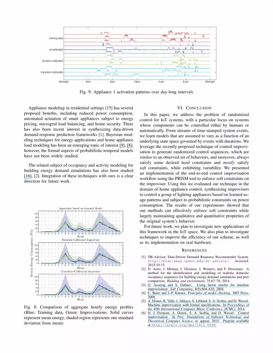
Finally, in Figure 9, we show several day-long tracesfrom the three improvisers together with time-aligned ex-cerpts from the training data. Note that the uncalibratedimprovisations are visually quite similar to the trainingdata, illustrating the quality of the EDHMM as a model.The calibrated improvisations are also qualitatively similarto the training data, but somewhat sparser as we wouldexpect from enforcing constraints on power consumption.This demonstrates how our model calibration techniques areeffective at enforcing soft constraints without too drasticallychanging the behavior of the system.
V. RELATED WORK
Control improvisation is an automata-theoretic problemthat was formally defined and analyzed in [6], and appliedto the automatic improvisation of music in [5].
Midnight 4am 8am 12pm 4 pm 8 pm Midnight
transition-calibrated
duration-calibrated
uncalibrated
training data
Fig. 9: Appliance 1 activation patterns over day-long intervals
Appliance modeling in residential settings [15] has severalproposed benefits, including reduced power consumption,automated actuation of smart appliances subject to energypricing, microgrid load balancing, and home security. Therehas also been recent interest in synthesizing data-drivendemand-response prediction frameworks [1]. Bayesian mod-eling techniques for energy applications and home applianceload modeling has been an emerging topic of interest [9], [8];however, the formal aspects of probabilistic temporal modelshave not been widely studied.
The related subject of occupancy and activity modeling forbuilding energy demand simulations has also been studied[16], [2]. Integration of these techniques with ours is a cleardirection for future work.
Fig. 8: Comparison of aggregate hourly energy profiles(Blue: Training data, Green: Improvisations. Solid curvesrepresent mean energy, shaded region represents one standarddeviation from mean)
VI. CONCLUSION
In this paper, we address the problem of randomizedcontrol for IoT systems, with a particular focus on systemswhose components can be controlled either by humans orautomatically. From streams of time-stamped system events,we learn models that are assumed to vary as a function of anunderlying state space governed by events with durations. Weleverage the recently-proposed technique of control improvi-sation to generate randomized control sequences, which aresimilar to an observed set of behaviors, and moreover, alwayssatisfy some desired hard constraints and mostly satisfysoft constraints, while exhibiting variability. We presentedan implementation of the end-to-end control improvisationworkflow using the PRISM tool to enforce soft constraints onthe improviser. Using this we evaluated our technique in thedomain of home appliance control, synthesizing improvisersto control a group of lighting appliances based on learned us-age patterns and subject to probabilistic constraints on powerconsumption. The results of our experiments showed thatour methods can effectively enforce soft constraints whilelargely maintaining qualitative and quantitative properties ofthe original system’s behavior.
For future work, we plan to investigate new applications ofthis framework in the IoT space. We also plan to investigatetechniques to improve the efficiency of our scheme, as wellas its implementation on real hardware.
REFERENCES
[1] DR-Advisor: Data-Driven Demand Response Recommender System.http://mlab.seas.upenn.edu/dr-advisor/. Accessed:2015-10-15.
[2] D. Aerts, J. Minnen, I. Glorieux, I. Wouters, and F. Descamps. Amethod for the identification and modelling of realistic domesticoccupancy sequences for building energy demand simulations and peercomparison. Building and environment, 75:67–78, 2014.
[3] G. Assayag and S. Dubnov. Using factor oracles for machineimprovisation. Soft Computing, 8(9):604–610, 2004.
[4] C. Baier and J.-P. Katoen. Principles of model checking. MIT Press,2008.
[5] A. Donze, R. Valle, I. Akkaya, S. Libkind, S. A. Seshia, and D. Wessel.Machine improvisation with formal specifications. In Proceedings ofthe 40th International Computer Music Conference (ICMC), 2014.
[6] D. J. Fremont, A. Donze, S. A. Seshia, and D. Wessel. Controlimprovisation. In Proc. Foundations of Software Technology andTheoretical Computer Science, to appear, 2015. Preprint availableat http://arxiv.org/abs/1411.0698.

[7] C. Gamarra and J. M. Guerrero. Computational optimization tech-niques applied to microgrids planning: a review. Renewable andSustainable Energy Reviews, 48:413–424, 2015.
[8] Z. Guo, Z. J. Wang, and A. Kashani. Home appliance load modelingfrom aggregated smart meter data. Power Systems, IEEE Transactionson, 30(1):254–262, 2015.
[9] Z. Kang, M. Jin, and C. J. Spanos. Modeling of end-use energyprofile: An appliance-data-driven stochastic approach. arXiv preprintarXiv:1406.6133, 2014.
[10] J. Kelly and W. Knottenbelt. The UK-DALE dataset, domesticappliance-level electricity demand and whole-house demand from fiveUK homes. 2(150007), 2015.
[11] M. Kwiatkowska, G. Norman, and D. Parker. PRISM 4.0: Verifi-cation of probabilistic real-time systems. In G. Gopalakrishnan andS. Qadeer, editors, Proc. 23rd International Conference on ComputerAided Verification (CAV’11), volume 6806 of LNCS, pages 585–591.Springer, 2011.
[12] E. Lee, A. Sangiovanni-Vincentelli, et al. A framework for comparingmodels of computation. Computer-Aided Design of Integrated Circuitsand Systems, IEEE Transactions on, 17(12):1217–1229, 1998.
[13] L. Rabiner. A tutorial on hidden Markov models and selected applica-tions in speech recognition. Proceedings of the IEEE, 77(2):257–286,1989.
[14] M. Strelec, K. Macek, and A. Abate. Modeling and simulationof a microgrid as a stochastic hybrid system. In Innovative SmartGrid Technologies (ISGT Europe), 2012 3rd IEEE PES InternationalConference and Exhibition on, pages 1–9. IEEE, 2012.
[15] L. G. Swan and V. I. Ugursal. Modeling of end-use energy con-sumption in the residential sector: A review of modeling techniques.Renewable and sustainable energy reviews, 13(8):1819–1835, 2009.
[16] U. Wilke, F. Haldi, J.-L. Scartezzini, and D. Robinson. A bottom-up stochastic model to predict building occupants’ time-dependentactivities. Building and Environment, 60:254–264, 2013.
[17] S.-Z. Yu. Hidden semi-markov models. Artificial Intelligence,174(2):215–243, 2010.