considerations for radio frequency fingerprinting across
TRANSCRIPT

�����������������
Citation: Gutierrez del Arroyo, J.A.;
Borghetti, B.J.; Temple, M.A.
Considerations for Radio Frequency
Fingerprinting across Multiple
Frequency Channels. Sensors 2022, 22,
2111. https://doi.org/10.3390/
s22062111
Academic Editors: William Chris
Headley and Alan Michaels
Received: 23 January 2022
Accepted: 4 March 2022
Published: 9 March 2022
Publisher’s Note: MDPI stays neutral
with regard to jurisdictional claims in
published maps and institutional affil-
iations.
Copyright: © 2022 by the authors.
Licensee MDPI, Basel, Switzerland.
This article is an open access article
distributed under the terms and
conditions of the Creative Commons
Attribution (CC BY) license (https://
creativecommons.org/licenses/by/
4.0/).
sensors
Article
Considerations for Radio Frequency Fingerprinting acrossMultiple Frequency ChannelsJose A. Gutierrez del Arroyo * , Brett J. Borghetti and Michael A. Temple
Department of Electrical and Computer Engineering, Air Force Institute of Technology,Wright-Patterson AFB, OH 45433, USA; [email protected] (B.J.B.); [email protected] (M.A.T.)* Correspondence: [email protected]
Abstract: Radio Frequency Fingerprinting (RFF) is often proposed as an authentication mechanismfor wireless device security, but application of existing techniques in multi-channel scenarios islimited because prior models were created and evaluated using bursts from a single frequencychannel without considering the effects of multi-channel operation. Our research evaluated themulti-channel performance of four single-channel models with increasing complexity, to include asimple discriminant analysis model and three neural networks. Performance characterization usingthe multi-class Matthews Correlation Coefficient (MCC) revealed that using frequency channelsother than those used to train the models can lead to a deterioration in performance from MCC > 0.9(excellent) down to MCC < 0.05 (random guess), indicating that single-channel models may notmaintain performance across all channels used by the transmitter in realistic operation. We proposeda training data selection technique to create multi-channel models which outperform single-channelmodels, improving the cross-channel average MCC from 0.657 to 0.957 and achieving frequencychannel-agnostic performance. When evaluated in the presence of noise, multi-channel discriminantanalysis models showed reduced performance, but multi-channel neural networks maintained orsurpassed single-channel neural network model performance, indicating additional robustness ofmulti-channel neural networks in the presence of noise.
Keywords: RF machine learning; deep learning; RF fingerprinting; RFF; specific emitter identification;wireless security
1. Introduction
Physical-layer emitter identification, known as RFF or Specific Emitter Identifica-tion (SEI), is often proposed as a means to bolster communications security [1]. Theunderlying theory is that the manufacturing processes used for chip components createhardware imperfections that make each emitter unique, irrespective of brand, model, or se-rial number. These hardware imperfections are akin to human biometrics (e.g., fingerprints)in that they are distinctive and measureable. Imperfections cause small distortions to theemissions of idealized signals, and those signal distortions can be learned by MachineLearning (ML) models to identify emitters solely from their emissions. This is particu-larly useful for communications security applications where the reported bit-level identity(e.g., MAC Address, Serial Number) of a device cannot or should not be implicitly trusted.Here, RFF can serve as a secondary out-of-band method for identity verification.
Prior related RFF research has trained ML models to identify devices by using burstsreceived on a single frequency channel. However, modern communications protocolsoften employ multiple frequency channels to enable simultaneous users and interferenceavoidance. For example, WiFi (IEEE 802.11 b/g/n) [2] subdivides the 2.4 GHz ISM band into11 × 20 MHz overlapping channels, ZigBee [3] and Wireless Highway Addressable RemoteTransducer (WirelessHART) [4] (i.e., IEEE 802.15.4-based protocols) use the same frequency
Sensors 2022, 22, 2111. https://doi.org/10.3390/s22062111 https://www.mdpi.com/journal/sensors
Sensors 2022, 22, 2111 2 of 21
band but divide it into 15 × 5 MHz non-overlapping channels [5], and Bluetooth [6] usesan even more granular division of 80 × 1 MHz non-overlapping channels.
When the channel changes, the carrier frequency used by both the transmitter andreceiver shifts to the center of the new channel. This change in carrier frequency affects thesignal distortions because radio hardware components such as Phase-Locked Loops (PLLs),amplifiers, and antennas operate irregularly at different frequencies. Furthermore, theRadio Frequency (RF) environment also varies with frequency channel because differ-ent sources of interference are present at different frequencies. Since most RFF researchpredominantly considers bursts received on a single channel, it is not clear whether theperformance achieved by those research efforts generally extends to multiple frequencychannel operation.
For instance, when researchers in [7–9] collected ZigBee signals, they configured theirreceivers to capture a narrow bandwidth centered on a single carrier frequency. They usedthose collections to train RFF models and tested their models on sequestered data fromthe same collections. No evidence was provided showing that the authors verified modelperformance across all channels.
In works providing single channel demonstrations, channel carrier frequency detailsare often omitted, given that the RF signals are commonly down-converted to accommodatebaseband fingerprint generation. For example, ZigBee research in [10–13], and similarly,WirelessHART research in [14], cited the collection bandwidth but omitted carrier frequencyinformation. Furthermore, from an experimental perspective, it is more time-consuming tocollect signals across multiple carrier frequencies, given the narrow RF bandwidth limita-tions of commonly accessible Software-Defined Radios (SDRs). Therefore, the omissionof carrier frequency information suggests that researchers in [10–14] did not consider theeffects of multi-channel operation.
Finally, there are researchers who implicitly use collections from multiple carrierfrequencies but make no explicit declaration in their work. For instance, any researchersusing the Defense Advanced Research Projects Agency (DARPA) Radio Frequency MachineLearning (RFML) WiFi dataset, such as [15–17], have the ability to account for multiplefrequency channels because collections for that dataset were performed with a wide band-width. It is not clear whether [15–17] deliberately considered frequency channel whenselecting training and evaluation datasets.
To our knowledge, no prior work has considered the sensitivity of RFF performance todifferent frequency channels; our results suggest that frequency channel must be considered.Signal bursts were collected using a wideband SDR receiver, which captured signals fromeight IEEE 802.15.4-based devices communicating across 15 frequency channels. Eachindividual burst was filtered and categorized based on the frequency channel withinwhich it was received. RFF models were trained and tested using data from differentchannel combinations to evaluate the effects of frequency channel to performance, whichwas reported using the multi-class MCC. Machine learning models included a MultipleDiscriminant Analysis/Maximum Likelihood (MDA/ML) model with expert-designedfeatures, a shallow fully-connected Artificial Neural Network (ANN), a Low-CapacityConvolutional Neural Network (LCCNN), and a High-Capacity Convolutional NeuralNetwork (HCCNN).
The key contributions of our work include:
• A first-of-its-kind evaluation of the sensitivity of single-channel models to multi-channel datasets. The evaluation suggests that failing to account for frequency channelduring training can lead to a deterioration in performance from MCC > 0.9 (excel-lent) down to MCC < 0.05 (random guess), indicating that single-channel modelperformance from previous RFF research should not be expected to extend to themulti-channel case (Experiment A).
• A training data selection technique to construct multi-channel models that can outper-form single-channel models, with average cross-channel MCC improving from 0.657to 0.957. The findings indicate that frequency-agnostic variability can be learned from
Sensors 2022, 22, 2111 3 of 21
a small subset of channels and can be leveraged to improve the generalizability of RFFmodels across all channels (Experiment B).
• An assessment of multi-channel models against Additive White Gaussian Noise(AWGN) that demonstrated the advantage of multi-channel models in noise perfor-mance depended on model type and noise level. Multi-channel neural networks ap-proximately maintained or surpassed single-channel performance, but multi-channelMDA/ML models were consistently outperformed by their single-channel counter-parts (Experiment C).
The rest of this paper is structured as follows: an overview of the state-of-the-art inRFF is provided in Section 1.1, and assumptions and limitations of this research are coveredin Section 1.2. Our wideband data collection technique is described in Section 2, includinghow the data were processed for RFF model training. Methodology and results for thethree experiments are detailed in Section 3, and study conclusions and potential futurework are presented in Section 4.
1.1. Related Work
RFF is fundamentally an ML classification problem, where discriminative features areleveraged to distinguish individual devices. Generation and down-selection of the best fea-tures remains an open area of research [18]. For instance, researchers have proposed an en-ergy criterion-based technique [19] and a transient duration-based technique [20] to detectand extract features from the transient region of the signal during power-on. Researchersin [14] extract features from the signal preamble region, focusing on down-selecting statisti-cal features to reduce computational overhead while maintaining classification accuracy.Yet another technique presented in [21] extracts features from a 2-dimensional representa-tion of the time series data. Commonly, researchers avoid feature selection altogether byingesting time series data directly into Convolutional Neural Networks (CNNs), whichcan be trained to learn the best feature set to be used for the ML task. CNNs have beenrecently used to classify a large number of devices across a wide swath of operationalconditions [17], to verify claimed identity against a small pool of known devices [9], and tomeasure identifiable levels of I-Q imbalance deliberately injected by the transmitter [15].
Another area of research focuses on bolstering the practicality of deploying RFFmechanisms in operational environments. Notably, ref. [22] explores how neural net-works might be pruned to reduce their size and complexity, enabling their deploymentto resource-constrained edge devices. Researchers in [23] tackle the need to retrain RFFmodels whenever a new device is added to the network by employing Siamese Networks,effectively aiding model scalability through one-shot learning. Our work contributes to thiseffort by comparing performance across four model types with increased levels of complex-ity, including an expert-feature-based MDA/ML model, a shallow ANN, a low-capacityCNN, and a high-capacity CNN.
Finally, the sensitivity to deployment variability is considered extensively in recentworks. For instance, variability stemming from time, location, and receiver configura-tion are studied extensively in [24], and variability stemming from the RF environmentis evaluated in depth by [25,26]. Often, the goal is to remove or reduce environmentaleffects to bolster classification accuracy, which can be done through data augmentation [27],transmitter-side pre-filtering [28], deliberate injection of I-Q imbalance at the transmit-ter [15], and through receiver-side channel equalization [17].
Our work extends the research in deployment variability by exploring the impactto model performance from the use of different frequency channels. Consistent with theworks by [24,25], we concluded that evaluating models under conditions that are differentfrom training conditions leads to negative impacts to RFF performance. Like [27], we foundthat adding more variability in our training made the models more generalizable, even toconditions not seen during training.

Sensors 2022, 22, 2111 4 of 21
1.2. Assumptions and Limitations
RFF and SEI are broad areas of research that include everything from the fingerprintingof personal and industrial communications devices, to radar and satellite identification. Ourwork leverages communications devices, but it is likely that any transmitter which operatesacross multiple carrier frequencies would exhibit the effects highlighted in this research.
The protocol used in this study was WirelessHART, which implements the PHY-layer in the IEEE 802.15.4 specification. That specification divides the 2.4-GHz Industrial,Scientific and Medical (ISM) band into 15 × 5 MHz channels, each with a different carrierfrequency. It is not clear whether the performance improvements of the multi-channelmodels shown in this research depend on the bandwidth of the frequency channel. Forinstance, models for Bluetooth, which employs narrower 80 × 1 MHz channels, may needmore frequency channels or further-spaced channels in the training set to achieve the samelevels of performance improvements. The impact of channel bandwidth to multi-channelmodels is left as future work.
Another key WirelessHART feature is that it allows the use of mesh networking,whereby each device can act as a relay of data for neighboring devices. Mesh networking isalso becoming increasingly popular in home automation, particularly with the adoption ofnew Internet of Things (IoT)-centric protocols such as Thread [29]. The distributed natureof those networks poses a challenge in RFF because there is no centralized endpoint withwhich all other devices communicate, so there is no ideal centralized location to place theRFF receiver. Our work is limited to the centralized configuration, which assumes that allWirelessHART devices communicate directly with the gateway. Configurations to handlemesh-networking, which could include multi-receiver systems or edge-based RFF, shouldbe explored in future work.
Although our work is limited to preamble-based fingerprinting, in part due to its recentsuccess in classifying WirelessHART devices [13], another highly researched technique istransient-based fingerprinting. Transient-based fingerprinting employs features related tohow a device becomes active in preparation for transmission, which has proven fruitful forthe purpose of device identification [19,20]. It is likely that transient-based detection willalso be affected by carrier frequency, given that the same radio components persist in thetransmit chain. Regardless, the study of the effects of frequency channel to transient-basedfingerprinting is an interesting area of future work.
In the wideband collection for this work, only one WirelessHART device was config-ured to communicate at a time. Under real operational conditions, multiple devices wouldbe able to communicate simultaneously on separate frequency channels, introducing thepotential for Adjacent Channel Interference (ACI). ACI occurs when energy emitted onone frequency channel leaks into adjacent frequency channels. At a minimum, this energyleakage could raise the noise floor, reducing the Signal-to-Noise Ratio (SNR) and potentiallydegrading model performance. A study of the specific effects of ACI to model performanceis left as future work.
In the end, our goal was to demonstrate that frequency channel can have a sig-nificant effect on RFF models in the hopes of encouraging future researchers to take itinto consideration.
2. Data Collection
A multi-channel WirelessHART dataset was collected and validated for the purposeof this study. Precautions were taken to minimize the effects stemming from the RFenvironment and receiver, as our focus was the study of transmitter effects. This Sectioncovers the methodology used for collection and pre-processing and includes a descriptionof the training, validation, and evaluation dataset(s).
2.1. WirelessHART Communications Protocol
The WirelessHART communications protocol, used by industrial sensors to transmitstateful information (e.g., temperature, humidity, voltage, etc.) between industrial sensors
Sensors 2022, 22, 2111 5 of 21
and to human-machine interfaces, implements the Offset-Quadrature Phase Shift Key-ing (O-QPSK) physical layer from IEEE 802.15.4, the standard for low-rate personal areanetworks [5]. This is the same standard employed by ZigBee, another common IoT protocol;many RF chips designed for WirelessHART are also compatible with ZigBee applications.WirelessHART uses the first 15 channels defined by the standard on the 2.4 GHz ISM bandand employs a pseudo-random frequency hopping scheme, where subsequent transmis-sions are sent on different frequency channels. Although the channel numbering given byIEEE 802.15.4 ranges from 11 through 25, we arbitrarily number our channels 0 through 14.Then, for a given channel i ∈ [0, 14], its center frequency is fc(i) = 2405 + i× 5 MHz, andits bandwidth is ( fc − 2.5, fc + 2.5) MHz.
WirelessHART was selected as the candidate protocol for collection for several reasons.First, the IEEE 802.15.4-based protocol is representative of many of the basic low-powerIoT devices being deployed across the globe at an exponentially increasing rate. Second,it operates in a common frequency band using a manageable number of channels. Andfinally, recent research in [14] employed MDA/ML using the same WirelessHART devicesused in our research, providing a baseline for performance comparison.
2.2. Collection Technique
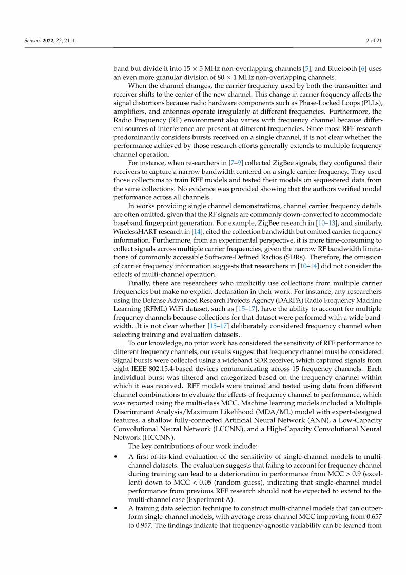
Figure 1 envisions how an RFF-based authentication mechanism might be deployed forWirelessHART. In this configuration, a centrally-located wideband SDR passively capturesbursts sent between the WirelessHART sensors and the gateway. Those bursts are offloadedto a monitoring application, which performs RFF and validates the claimed identity of thecommunicating device. Once the burst is validated, the information contained within it isconsidered trusted. Our collection setup is based on this conceptual configuration.
WirelessHARTGateway
Monitoring Application(RFF/Device Verification)
Critical Production Application or HMI
Wideband SDR
TX/RX
WirelessHARTSensors
RX RX
Workstation
Verified Data
Data to Verify
Raw Bursts
Process Data
Figure 1. Envisioned use case for RFF-based authentication of WirelessHART devices. Our experi-mental setup mimicked this configuration.
WirelessHART devices were allowed to communicate directly with the WirelessHARTgateway one at a time, while an SDR captured device emissions. During collection, thedevice was placed 8 ft. from the gateway, and the SDR antenna was positioned 18 in. fromthe device. The eight devices observed are listed in Table 1 and included four SiemensAW210 [30] and four Pepperl+Fuchs Bullet [31] devices.
Bursts were captured using a USRP X310 with a 100 MHz bandwidth centered at2.440 GHz, enabling simultaneous collection of all 15 WirelessHART channels. Burstdetection for the wideband data was performed “on-the-fly” by thresholding the powerof the received signal. This enabled the collector to be efficient with its limited hard diskspace. In particular, given a received signal, c[n] = cI [n] + jcQ[n], the instantaneous powerwas calculated as |c[n]|2 = (cI [n])2 + (cQ[n])2. A 100-sample moving average was thenused to detect the start and end of each burst using empirically-set thresholds. Buffers of10 K complex I-Q samples were added before the start and after the end of the burst to aidin SNR approximation, and each detected burst was saved to a new file.
Sensors 2022, 22, 2111 6 of 21
Table 1. Serial numbers and source addresses for the eight WirelessHART devices.
Device Number Manufacturer Serial Number Hex Source Address(Assigned by Gateway)
0 Siemens 003095 00021 Siemens 003159 00052 Siemens 003097 00063 Siemens 003150 00034 Pepperl+Fuchs 1A32DA 00045 Pepperl+Fuchs 1A32B3 00076 Pepperl+Fuchs 1A3226 00087 Pepperl+Fuchs 1A32A4 0009
Three precautions were taken in an attempt to minimize effects from the RF environ-ment. First, collections were done within a ranch-style suburban household, far away fromother wireless emitters relative to the distance between emitter and receiver. Second, allcollections were performed in the same physical location, meaning that any RF effectsdue to interference with nearby non-emitters would likely manifest in the same way forall devices. Finally, collections were performed in sets of 10 K bursts, started at randomtimes during the day throughout the course of two weeks. This ensured any potentialtime-dependent sources of interference were well distributed across devices.
Collecting data in sets of 10 K bursts also forced the WirelessHART gateway to assigna new frequency hopping scheme to each device when it re-established communicationwith the gateway (per the WirelessHART specification [4]). This resulted in a relativelyeven distribution of bursts across the 15 frequency channels.
2.3. Burst Validation
Our approach for burst detection did not guarantee that the received signal camefrom the expected WirelessHART device; it could be the case that strong interferencetriggered the burst detector. Further protocol-specific analysis was performed to ensurethe validity of each collected burst. The most straightforward way to do this was todetect and verify the structure of the preamble, and subsequently read message-levelbits to verify that the transmitted source address corresponded to that listed in Table 1.The process of burst validation consisted of Frequency Correction, Low-Pass Filtering,WirelessHART Preamble Detection and Verification, Phase Correction, and Message Parsingand Address Verification.
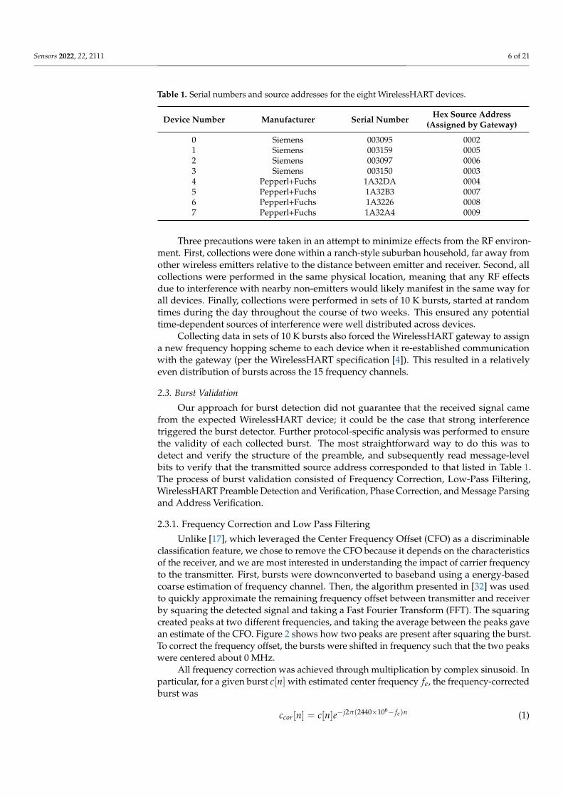
2.3.1. Frequency Correction and Low Pass Filtering
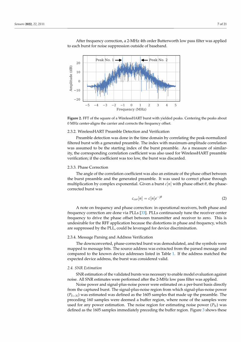
Unlike [17], which leveraged the Center Frequency Offset (CFO) as a discriminableclassification feature, we chose to remove the CFO because it depends on the characteristicsof the receiver, and we are most interested in understanding the impact of carrier frequencyto the transmitter. First, bursts were downconverted to baseband using a energy-basedcoarse estimation of frequency channel. Then, the algorithm presented in [32] was usedto quickly approximate the remaining frequency offset between transmitter and receiverby squaring the detected signal and taking a Fast Fourier Transform (FFT). The squaringcreated peaks at two different frequencies, and taking the average between the peaks gavean estimate of the CFO. Figure 2 shows how two peaks are present after squaring the burst.To correct the frequency offset, the bursts were shifted in frequency such that the two peakswere centered about 0 MHz.
All frequency correction was achieved through multiplication by complex sinusoid. Inparticular, for a given burst c[n] with estimated center frequency fe, the frequency-correctedburst was
ccor[n] = c[n]e−j2π(2440×106− fe)n (1)
Sensors 2022, 22, 2111 7 of 21
After frequency correction, a 2-MHz 4th order Butterworth low pass filter was appliedto each burst for noise suppression outside of baseband.
5 4 3 2 1 0 1 2 3 4 5Frequency (MHz)
20
10
0
10
20
Ampl
itude
(dB
)
Peak No. 1 Peak No. 2
Figure 2. FFT of the square of a WirelessHART burst with yielded peaks. Centering the peaks about0 MHz center-aligns the carrier and corrects the frequency offset.
2.3.2. WirelessHART Preamble Detection and Verification
Preamble detection was done in the time domain by correlating the peak-normalizedfiltered burst with a generated preamble. The index with maximum-amplitude correlationwas assumed to be the starting index of the burst preamble. As a measure of similar-ity, the corresponding correlation coefficient was also used for WirelessHART preambleverification; if the coefficient was too low, the burst was discarded.
2.3.3. Phase Correction
The angle of the correlation coefficient was also an estimate of the phase offset betweenthe burst preamble and the generated preamble. It was used to correct phase throughmultiplication by complex exponential. Given a burst c[n] with phase offset θ, the phase-corrected burst was
ccor[n] = c[n]e−jθ (2)
A note on frequency and phase correction: in operational receivers, both phase andfrequency correction are done via PLLs [33]. PLLs continuously tune the receiver centerfrequency to drive the phase offset between transmitter and receiver to zero. This isundesirable for the RFF application because the distortions in phase and frequency, whichare suppressed by the PLL, could be leveraged for device discrimination.
2.3.4. Message Parsing and Address Verification
The downconverted, phase-corrected burst was demodulated, and the symbols weremapped to message bits. The source address was extracted from the parsed message andcompared to the known device addresses listed in Table 1. If the address matched theexpected device address, the burst was considered valid.
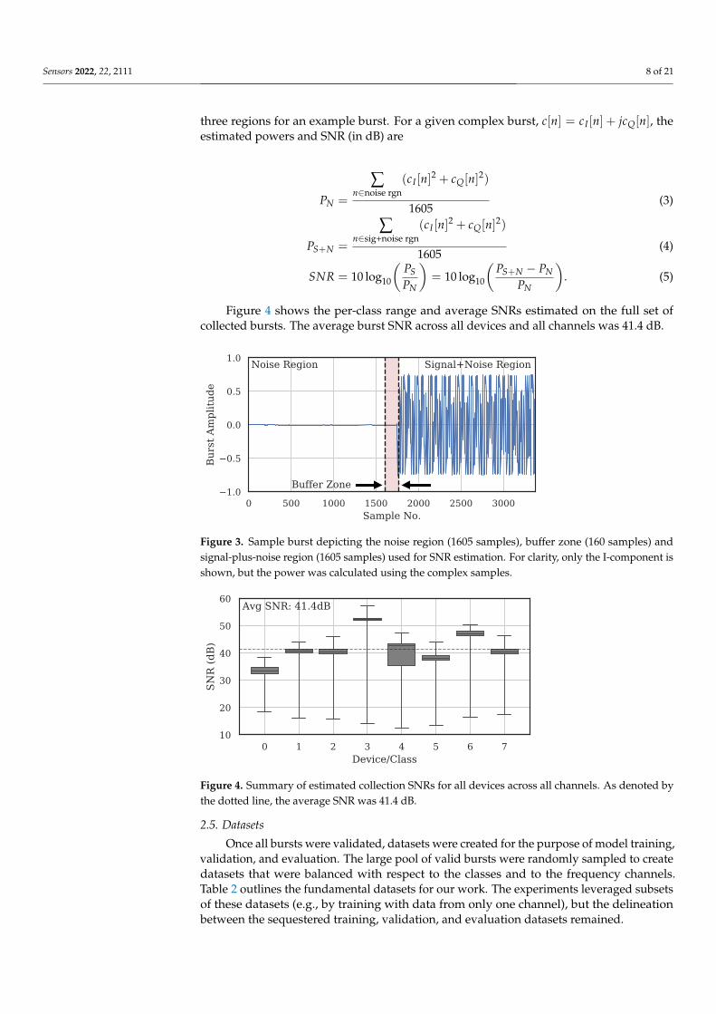
2.4. SNR Estimation
SNR estimation of the validated bursts was necessary to enable model evaluation againstnoise. All SNR estimates were performed after the 2-MHz low pass filter was applied.
Noise power and signal-plus-noise power were estimated on a per-burst basis directlyfrom the captured burst. The signal-plus-noise region from which signal-plus-noise power(PS+N) was estimated was defined as the 1605 samples that made up the preamble. Thepreceding 160 samples were deemed a buffer region, where none of the samples wereused for any power estimation. The noise region for estimating noise power (PN) wasdefined as the 1605 samples immediately preceding the buffer region. Figure 3 shows these
Sensors 2022, 22, 2111 8 of 21
three regions for an example burst. For a given complex burst, c[n] = cI [n] + jcQ[n], theestimated powers and SNR (in dB) are
PN =
∑n∈noise rgn
(cI [n]2 + cQ[n]2)
1605(3)
PS+N =
∑n∈sig+noise rgn
(cI [n]2 + cQ[n]2)
1605(4)
SNR = 10 log10
(PSPN
)= 10 log10
(PS+N − PN
PN
). (5)
Figure 4 shows the per-class range and average SNRs estimated on the full set ofcollected bursts. The average burst SNR across all devices and all channels was 41.4 dB.
0 500 1000 1500 2000 2500 3000Sample No.
1.0
0.5
0.0
0.5
1.0
Bur
st A
mpl
itude
Noise Region Signal+Noise Region
Buffer Zone
Figure 3. Sample burst depicting the noise region (1605 samples), buffer zone (160 samples) andsignal-plus-noise region (1605 samples) used for SNR estimation. For clarity, only the I-component isshown, but the power was calculated using the complex samples.
0 1 2 3 4 5 6 7Device/Class
10
20
30
40
50
60
SNR
(dB
)
Avg SNR: 41.4dB
Figure 4. Summary of estimated collection SNRs for all devices across all channels. As denoted bythe dotted line, the average SNR was 41.4 dB.
2.5. Datasets
Once all bursts were validated, datasets were created for the purpose of model training,validation, and evaluation. The large pool of valid bursts were randomly sampled to createdatasets that were balanced with respect to the classes and to the frequency channels.Table 2 outlines the fundamental datasets for our work. The experiments leveraged subsetsof these datasets (e.g., by training with data from only one channel), but the delineationbetween the sequestered training, validation, and evaluation datasets remained.

Sensors 2022, 22, 2111 9 of 21
Table 2. Fundamental datasets used in this work, broken down by class and channel.
No. of Observations Training Set Validation Set Evaluation Set
per Device per Channel 5000 500 1000per Channel 40,000 4000 8000per Class 75,000 7500 15,000in Total 600,000 60,000 120,000
3. Experiments
Three experiments were designed to (i) assess the sensitivity of single-channel modelsto a multi-channel dataset, (ii) determine whether carefully-constructed multi-channelmodels generalized better than single-channel models, and (iii) determine whether multi-channels models gained more resiliency to noise. This section provides a description ofthe four models used across all tests, followed by individual methodologies, results, andanalyses for the three experiments.
3.1. RFF Models
Four typical RFF models with varying levels of complexity were selected as candidatesfor experimentation in this work. All four model types were used in all three experiments.This section describes the structure of each model in detail.
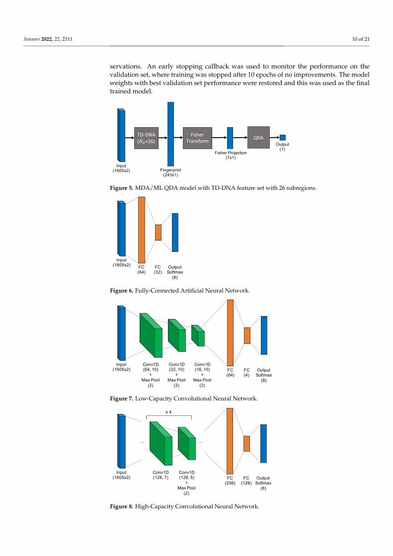
1. Multiple Discriminant Analysis/Maximum Likelihood. This model type leverages thecommonly-used Time-Domain Distinct Native Attribute (TD-DNA) feature set [10,34,35],as depicted in Figure 5, which was recently used by Rondeau et al. on single-channelWirelessHART bursts [14]. TD-DNA features are statistics calculated for a set of signalsubregions (defined by NR) after a number of signal transforms. The features aredimensionally reduced through Fisher Transform and fed in to a standard QuadraticDiscriminant Analysis (QDA) model for classification. Including dimensionalityreduction and discriminant analysis, the total number of trainable parameters is 1757.
2. Fully-Connected Artificial Neural Network. Figure 6 shows the ANN, which operateddirectly on raw complex I-Q burst data input to the network on two independent datapaths (one for I and one for Q). The two-dimensional input was flattened into a single3210-wide vector which was fed to the first fully-connected layer. Even with 207,848trainable parameters (10 times that of MDA/ML), this particular ANN was a shallow,low-complexity alternative to the other two neural networks.
3. Low-Capacity Convolutional Neural Network. Like the ANN, the LCCNN presentedin Figure 7 operated directly on raw complex I-Q burst data. The network comprisedeight Conv1D layers that applied a total of 112 digital filters and two fully-connectedlayers that mapped the filter output to a four-dimensional latent space. The Softmaxoutput layer was used for classification, where class prediction was determined bythe node with largest output value. Because of its convolutional layers, the LCCNN isable to add depth to the ANN with 232,156 trainable parameters.
4. High-Capacity Convolutional Neural Network. This high-capacity model was in-spired by ORACLE, a CNN that extracts and classifies injected I-Q imbalance [15].This model carried significantly more capacity, with 14 hidden layers comprisingfour pairs of 128-filter Conv1D layers that applied a total of 1024 digital filters, andtwo fully-connected layers that mapped the filter outputs to a 64-dimensional latentspace. Like in the LCCNN, the input layer contained two independent input paths,and the output Softmax layer contained one node for each of the eight classes inthis study. This is the most complex model, requiring 3,985,544 trainable parame-ters, approximately 20 times as many as the ANN and LCCNN. Figure 8 depictsthe HCCNN.
MDA/ML models were trained by fitting a QDA model onto the dimensionally-reduced TD-DNA features. All neural networks were trained using Stochastic GradientDescent with the Adam optimizer and learning rate of 1× 10⁻⁴, with batch size of 512 ob-
Sensors 2022, 22, 2111 10 of 21
servations. An early stopping callback was used to monitor the performance on thevalidation set, where training was stopped after 10 epochs of no improvements. The modelweights with best validation set performance were restored and this was used as the finaltrained model.
Input(1605x2) Fingerprint
(243x1)
Fisher Projection(7x1)
QDAOutput
(1)
TD-DNA(𝑁!=26)
Fisher Transform
Figure 5. MDA/ML QDA model with TD-DNA feature set with 26 subregions.
Input(1605x2) FC
(64)FC(32)
OutputSoftmax(8)
Figure 6. Fully-Connected Artificial Neural Network.
Input(1605x2)
Conv1D(64, 10)
+Max Pool
(2)
FC(64)
Conv1D(32, 10)
+Max Pool
(2)
Conv1D(16, 10)
+Max Pool
(2)
FC(4)
OutputSoftmax
(8)
Figure 7. Low-Capacity Convolutional Neural Network.
Input(1605x2)
Conv1D(128, 7) FC
(256)
Conv1D(128, 5)
+Max Pool
(2)
FC(128)
OutputSoftmax
(8)
x 4
… …
Figure 8. High-Capacity Convolutional Neural Network.

Sensors 2022, 22, 2111 11 of 21
3.2. Performance Metric: Matthews Correlation Coefficient (MCC)
Performance for RFF models is typically reported as per-class classification accuracy,which is the accuracy averaged across all classes. For K classes, per-class classificationaccuracy degrades to 1/K when models perform no better than random guess. It is thereforedifficult to grasp model performance without first knowing how many classes were usedto train the model. One way to address this problem is to standardize performance by thenumber of classes through the use of MCC.
MCC is a performance metric first designed for binary class classification models,derived by Matthews as a discrete version of the correlation coefficient [36]. An MCC valueof 1.0 indicates perfect correct model performance, 0.0 indicates performance no betterthan random guess, and −1.0 indicates perfect incorrect model performance. The multi-class case, derived by Gorodkin [37], preserves the −1.0 to 1.0 quantitative performancecharacteristics. For K classes, MCC is calculated as
MCC =
cs−∑k
pktk√s2 −∑
k(pk)
2√
s2 −∑k(tk)
2(6)
where tk is the number of occurrences for class k ∈ [0, 1, 2, . . . , K− 1], pk is the number oftimes class k was predicted, c is the total number of correct predictions, and s is the totalnumber of predictions [38]. For our experiments, we use K = 8 classes and report all modelperformance via MCC.
3.3. Experiment A: Single-Channel Models
The goal in this experiment was to determine whether the performance of modelstrained on a single channel (i.e., “single-channel models”) extends to other frequencychannels. To that end, single-channel models were evaluated against a dataset containingbursts from multiple channels, and the per-channel evaluation performance was reported.
3.3.1. Methodology
The training and validation datasets described in Section 2.5 were subdivided into15 subsets, one for each channel, yielding a total of 5 K training observations and 500 vali-dation observations per device in each subset. Then, the four models were trained witheach subset to create a total of 60 single-channel RFF models. All models were evaluatedon the full evaluation dataset described in Section 2.5, which contained bursts from all15 channels. MCC was calculated using Equation (6).
3.3.2. Results and Analysis
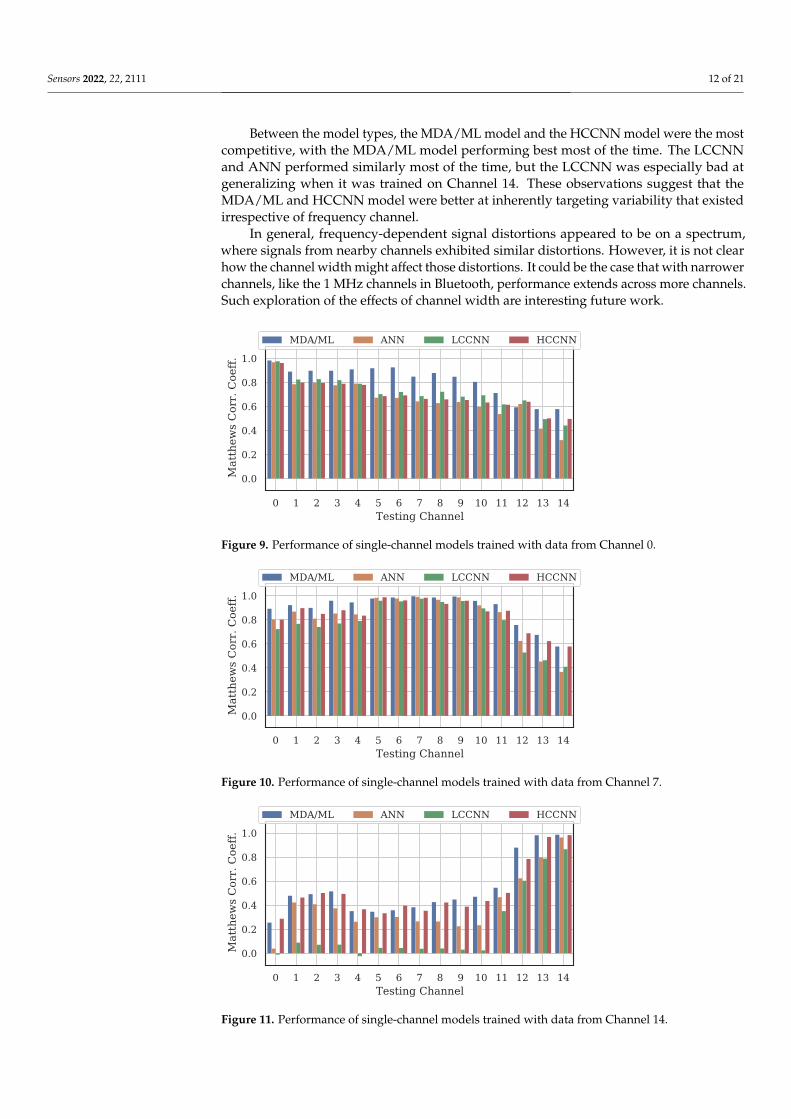
Figures 9–11 show the performance for single-channel models trained on data fromChannel 0, Channel 7 and Channel 14, respectively. Plots for the remaining single-channelmodels have been omitted for brevity, given these three figures are representative of theoverarching observations for this experiment. Performance was reported individually foreach channel in the evaluation set to show how well the models operated outside theirtraining scope. Note that performance always peaked at the channel on which the modelswere trained and deteriorated when the evaluation channel was farther away (in frequency)from the training channel.
As expected, none of the models generalized across all channels when trained on datafrom a single channel, but some models did generalize better than others. In particular,when the models were trained on data from Channel 7, they generalized well across a wideswath of channels (e.g., Channels 5–10), whereas when the models were trained on Channel14, performance only roughly generalized to Channel 13 and only for MCA/ML andHCCNN. In the worst case, signals from distant channels were classified by the Channel 14model with success no better than random guess.
Sensors 2022, 22, 2111 12 of 21
Between the model types, the MDA/ML model and the HCCNN model were the mostcompetitive, with the MDA/ML model performing best most of the time. The LCCNNand ANN performed similarly most of the time, but the LCCNN was especially bad atgeneralizing when it was trained on Channel 14. These observations suggest that theMDA/ML and HCCNN model were better at inherently targeting variability that existedirrespective of frequency channel.
In general, frequency-dependent signal distortions appeared to be on a spectrum,where signals from nearby channels exhibited similar distortions. However, it is not clearhow the channel width might affect those distortions. It could be the case that with narrowerchannels, like the 1 MHz channels in Bluetooth, performance extends across more channels.Such exploration of the effects of channel width are interesting future work.
0 1 2 3 4 5 6 7 8 9 10 11 12 13 14Testing Channel
0.0
0.2
0.4
0.6
0.8
1.0
Mat
thew
s C
orr.
Coe
ff.
MDA/ML ANN LCCNN HCCNN
Figure 9. Performance of single-channel models trained with data from Channel 0.
0 1 2 3 4 5 6 7 8 9 10 11 12 13 14Testing Channel
0.0
0.2
0.4
0.6
0.8
1.0
Mat
thew
s C
orr.
Coe
ff.
MDA/ML ANN LCCNN HCCNN
Figure 10. Performance of single-channel models trained with data from Channel 7.
0 1 2 3 4 5 6 7 8 9 10 11 12 13 14Testing Channel
0.0
0.2
0.4
0.6
0.8
1.0
Mat
thew
s C
orr.
Coe
ff.
MDA/ML ANN LCCNN HCCNN
Figure 11. Performance of single-channel models trained with data from Channel 14.

Sensors 2022, 22, 2111 13 of 21
Additionally, recall that the transmitter, RF environment, and receiver distortions werenot decoupled. Thus, it is possible that a non-trivial part of the variability between fre-quency channels was imposed by non-transmitter sources. Finding a way to decouple (or atleast reduce the coupling) across the three sources would enable more flexible applications(e.g., multi-receiver narrowband systems) and could help researchers more precisely targetthe signal alterations imposed by hardware components in the transmitter. Regardless ofits source, the variability must be considered to achieve good RFF performance.
A natural follow-up experiment was to include data from multiple channels in thetraining set to determine if this improved model generalizability. This experiment iscovered in the following Section.
3.4. Experiment B: Multi-Channel Models
The focus of Experiment A was to demonstrate that single-channel models did notalways perform well across all frequency channels. In Experiment B, the goal was todetermine whether including bursts from multiple channels during training improvesperformance. During training, we deliberately use data from an increasing number ofchannels, relatively spread throughout the 80 MHz band to create “multi-channel models.”These models were tested against the same evaluation set from Experiment A, whichincluded bursts from all 15 channels.
3.4.1. Methodology
The same four models presented in Section 3.1 were used in Experiment B. Trainingwas done using 11 datasets assembled from portions of the full training set described inSection 2.5, but special consideration was taken with respect to the number of observationsin training sets.
Generally, the performance of ML models is influenced by the number of observationsprovided during training. To enable comparison between multi-channel models fromExperiment B and single-channel models from Experiment A, the size of the trainingdatasets was limited to no more than 5000 observations per device (i.e., the size of trainingsets in Experiment A). Concretely, two-channel data subsets contained 2500 observationsper device per channel (5000 observations/device in total), three-channel data subsetscontained 1666 observations/device per channel (4998 observations/device), four-channelsubsets had 1250 observations per device per channel (5000 observations/device), and theall-channel (i.e., 15-channel) subset contained only 333 observations per device per channel(4995 observations/device). Channel combinations were selected to explore how channelcoverage impacted performance. The 11 data subsets used for Experiment B are listed inTable 3. Evaluation was done using the same dataset from Experiment A, which containedbursts from all 15 channels.
Table 3. Summary of datasets used for Experiment B.
No. of Chans. Chans. in Datasets Observations perChan. per Device
Observationsper Device Total
2 [0,14], [1,13], [2,12], [3,11] 2500 5000 40,0003 [0,7,14], [1,7,13], [2,7,12], [3,7,11] 1666 4998 39,9844 [0, 4, 10, 14], [1, 5, 9, 13] 1250 5000 40,000All [0,1,2,. . . ,14] 333 4995 39,960
3.4.2. Results and Analysis
A representative sample of the performance results for the multi-frequency modelsare depicted in Figures 12–15.
Comparing the Channel 14 single-channel models from Experiment A in Figure 11with the 2-channel models in Figure 12, it is immediately evident that adding even onemore channel to the training set improved generalizability, regardless of model type. Withthe addition of Channel 0 to the training set, the worst-case performance across all models
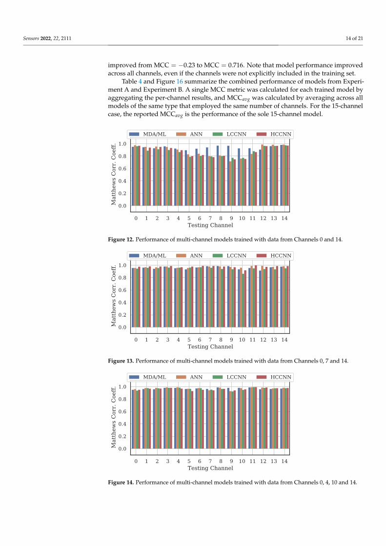
Sensors 2022, 22, 2111 14 of 21
improved from MCC = −0.23 to MCC = 0.716. Note that model performance improvedacross all channels, even if the channels were not explicitly included in the training set.
Table 4 and Figure 16 summarize the combined performance of models from Experi-ment A and Experiment B. A single MCC metric was calculated for each trained model byaggregating the per-channel results, and MCCavg was calculated by averaging across allmodels of the same type that employed the same number of channels. For the 15-channelcase, the reported MCCavg is the performance of the sole 15-channel model.
0 1 2 3 4 5 6 7 8 9 10 11 12 13 14Testing Channel
0.0
0.2
0.4
0.6
0.8
1.0
Mat
thew
s C
orr.
Coe
ff.
MDA/ML ANN LCCNN HCCNN
Figure 12. Performance of multi-channel models trained with data from Channels 0 and 14.
0 1 2 3 4 5 6 7 8 9 10 11 12 13 14Testing Channel
0.0
0.2
0.4
0.6
0.8
1.0
Mat
thew
s C
orr.
Coe
ff.
MDA/ML ANN LCCNN HCCNN
Figure 13. Performance of multi-channel models trained with data from Channels 0, 7 and 14.
0 1 2 3 4 5 6 7 8 9 10 11 12 13 14Testing Channel
0.0
0.2
0.4
0.6
0.8
1.0
Mat
thew
s C
orr.
Coe
ff.
MDA/ML ANN LCCNN HCCNN
Figure 14. Performance of multi-channel models trained with data from Channels 0, 4, 10 and 14.

Sensors 2022, 22, 2111 15 of 21
0 1 2 3 4 5 6 7 8 9 10 11 12 13 14Testing Channel
0.0
0.2
0.4
0.6
0.8
1.0
Mat
thew
s C
orr.
Coe
ff.
MDA/ML ANN LCCNN HCCNN
Figure 15. Performance of multi-channel models trained with data from all channels.
1 2 3 4 All (15)No. of Channels in Training Set
0.2
0.4
0.6
0.8
1.0
MC
Cav
g
MDA/ML ANN LCCNN HCCNN
Figure 16. Performance summary for all models as the number of channels in the training wasincreased. Trend lines represent MCCavg, and color bands represent the range of MCC values at thatnumber of training channels. Notably, all-channel performance was achieved with only four channelsincluded in the training set.
Two trends are evident from these metrics: (i) model performance generally improvedwhen channels were added to the training set, and (ii) the performance of 4-channel modelsapproached the performance of 15-channel models. Note that even the worst performingsingle-channel model type, i.e., the LCCNN, improved its MCCavg from 0.657 to 0.957with only three additional channels in the training set. The one exception was with theANN, for which the 15-channel MCCavg was 0.006 units lower than the 4-channel MCCavg.This small gap in performance might be attributed to the variability stemming from therandomized initial model weights before training, or from the fact that the 15-channel“average” included only one model—retraining the 15-channel ANN may yield slightlybetter results.
Table 4. Summary of MCCavg for all models from Experiments A and B. In general, MCC improvedas the number of channels in the training set were increased.
No. of ChannelsMCCavg
MDA/ML ANN LCCNN HCCNN
1 0.833 0.723 0.657 0.7422 0.943 0.857 0.823 0.8593 0.961 0.957 0.930 0.9504 0.967 0.970 0.957 0.958
15 (All) 0.974 0.964 0.967 0.958
Regardless, these trends again support the existence of frequency-irrespective vari-ability. Multi-channel models were better suited to learn that variability, even with limited
Sensors 2022, 22, 2111 16 of 21
(i.e., 4-channel) exposure to the spectrum. Furthermore, the MDA/ML model consistentlygeneralized better than its neural network counterparts, suggesting that the frequency-irrespective variability in our particular experimental setup can be effectively extractedthrough the TD-DNA fingerprint generation process.
In practice, it is desirable for RFF models to perform well across all frequency channels,but that is not the only requirement. Models should also perform well under the presence ofenvironmental noise. Thus, researchers often report model performance across multiple lev-els of noise, modeled as AWGN. Experiment C explores whether multi-channel models gainany performance advantages over single-channel models under varying noise conditions.
3.5. Experiment C: Gains in Noise Performance
The goal of the final experiment was to determine whether multi-channel modelsgained any performance advantages over single-channel models in noisy RF environments.Tested models included the Channel 7 single-channel models from Experiment A, andnew “all-channel/all-data” multi-channel models built exclusively for this experiment.All models were evaluated with bursts from Channel 7 with varying SNR levels adjustedsynthetically through the addition of power-scaled AWGN.
3.5.1. Methodology
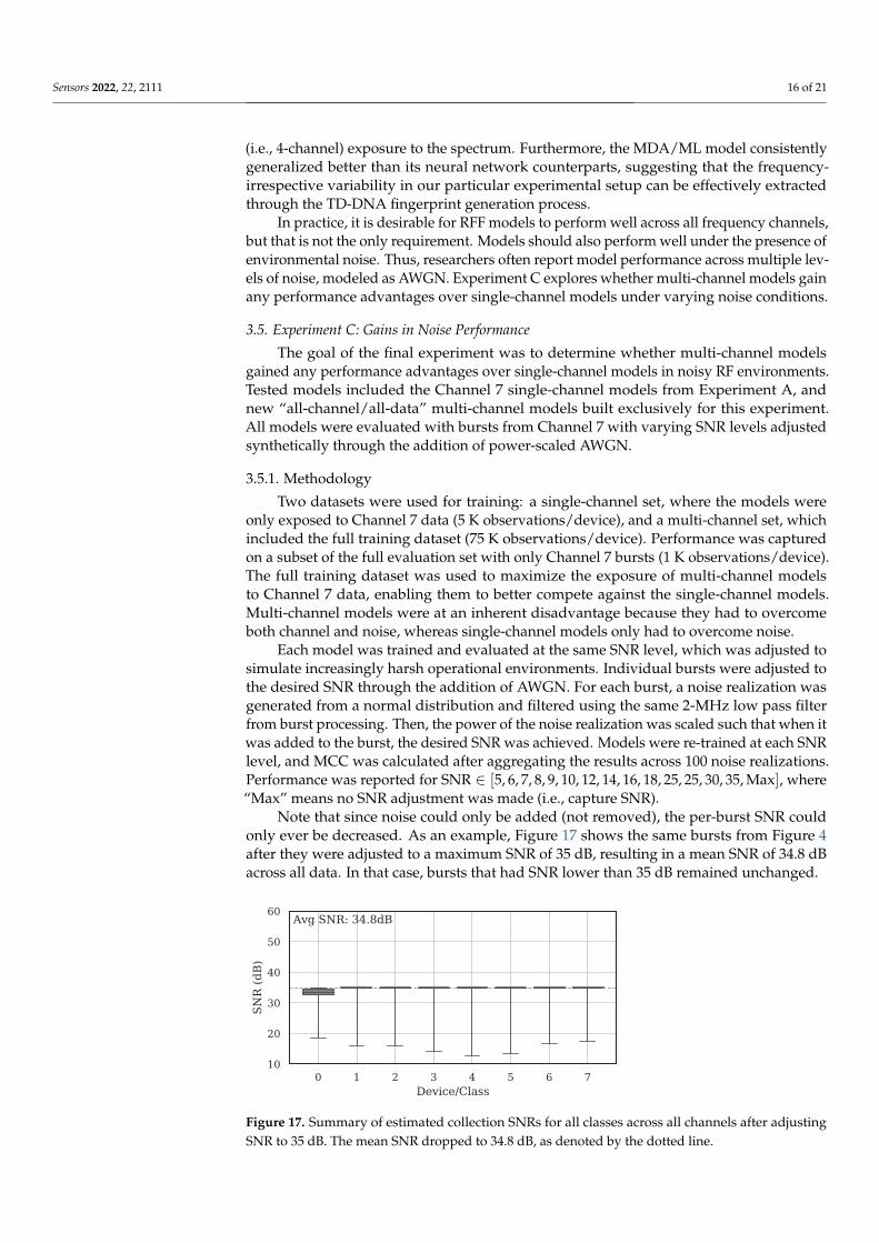
Two datasets were used for training: a single-channel set, where the models wereonly exposed to Channel 7 data (5 K observations/device), and a multi-channel set, whichincluded the full training dataset (75 K observations/device). Performance was capturedon a subset of the full evaluation set with only Channel 7 bursts (1 K observations/device).The full training dataset was used to maximize the exposure of multi-channel modelsto Channel 7 data, enabling them to better compete against the single-channel models.Multi-channel models were at an inherent disadvantage because they had to overcomeboth channel and noise, whereas single-channel models only had to overcome noise.
Each model was trained and evaluated at the same SNR level, which was adjusted tosimulate increasingly harsh operational environments. Individual bursts were adjusted tothe desired SNR through the addition of AWGN. For each burst, a noise realization wasgenerated from a normal distribution and filtered using the same 2-MHz low pass filterfrom burst processing. Then, the power of the noise realization was scaled such that when itwas added to the burst, the desired SNR was achieved. Models were re-trained at each SNRlevel, and MCC was calculated after aggregating the results across 100 noise realizations.Performance was reported for SNR ∈ [5, 6, 7, 8, 9, 10, 12, 14, 16, 18, 25, 25, 30, 35, Max], where“Max” means no SNR adjustment was made (i.e., capture SNR).
Note that since noise could only be added (not removed), the per-burst SNR couldonly ever be decreased. As an example, Figure 17 shows the same bursts from Figure 4after they were adjusted to a maximum SNR of 35 dB, resulting in a mean SNR of 34.8 dBacross all data. In that case, bursts that had SNR lower than 35 dB remained unchanged.
0 1 2 3 4 5 6 7Device/Class
10
20
30
40
50
60
SNR
(dB
)
Avg SNR: 34.8dB
Figure 17. Summary of estimated collection SNRs for all classes across all channels after adjustingSNR to 35 dB. The mean SNR dropped to 34.8 dB, as denoted by the dotted line.

Sensors 2022, 22, 2111 17 of 21
3.5.2. Results and Analysis
Figure 18, which depicts noise performance of the LCCNN models, is representativeof the results across all model types. As expected, MCCs for both the single- and multi-channel models worsened as SNR was decreased. To help determine whether multi-channelmodels gained an advantage against noise, we define a new metric, MCC∆, as the differencebetween multi-channel performance and single-channel performance for a given modeltype, i.e.,
MCC∆ = MCC(multi-channel)−MCC(single-channel), (7)
for which a positive MCC∆ implies better multi-channel performance. Figure 19 illustratesMCC∆ for the four models across varying SNR levels.
The advantage of multi-channel models depended on model type and SNR level. Athigh SNR levels (SNR > 20 dB), MCC∆ was generally stable for all model types. In thatregion, the multi-channel CNNs matched or beat single-channel CNNs, but the single-channelANNs and MDA/ML models bested their multi-channel counterparts. With mid-level SNRs(10 dB < SNR < 20 dB), MCC∆ for the three neural networks fluctuated between positive andnegative, suggesting no clear advantage for multi-channel models. Notably, single-channelMDA/ML models thrived in this region, surpassing multi-channel models by up to 0.13 units.Finally, at low SNR levels (SNR < 10 dB), multi-channel models for all four model typesshowed some advantage over single-channel models, though arguably, the performance inthis region was already too weak (MCC . 0.5) to be practical for RFF applications.
5 6 7 8 910 12 14 16 18 20 25 30 35MaxTesting SNR (dB)
0.00
0.25
0.50
0.75
1.00
Mat
thew
s C
orr.
Coe
ff.
Single-Channel (Ch. 7) Multi-Channel (All)
Figure 18. Performance of single-channel and multi-channel LCCNN models at varying SNRs.
5 6 7 8 910 12 14 16 18 20 25 30 35 MaxTesting SNR (dB)
-0.1
-0.05
0
0.05
0.1
MC
C
MDA/ML ANN LCCNN HCCNN
Figure 19. Performance difference between multi-channel models and single-channel models acrossvarying SNR levels, where MCC∆ > 0 implies better multi-channel performance. Multi-channelneural networks (i.e., CNNs and ANN) approximately maintained or outperformed their single-channel counterparts, but multi-channel MDA/ML models did not.
Sensors 2022, 22, 2111 18 of 21
For the neural networks (i.e., CNNs and ANN), the frequency-irrespective variabilitylearned by the multi-channel models enabled them to approximately maintain or surpasssingle-channel model performance. Conversely, the single-channel MDA/ML modelsconsistently outperformed their multi-channel counterparts in the presence of noise. Itcould be that frequency-specific variability, which was deliberately ignored by multi-channel models, allowed some of the single-channel MDA/ML models to overfit thetraining channel, giving them an advantage against random noise.
4. Conclusions and Future Work
Modern communications protocols often employ multiple frequency channels to enablesimultaneous user operation and mitigate adverse interference effects. Although recent RFFresearch targets devices that implement these protocols, the direct applicability of theseproof-of-concept works is generally limited given that they train RFF models using burstsreceived on a single channel. Because the signal distortions leveraged by RFF models arelinked to the radio hardware components, and those components operate irregularly acrossdifferent frequencies, practical RFF models must account for multiple frequency channels.Using WirelessHART signal bursts collected with a wideband SDR, our work demonstratedthat RFF model performance depends on the frequency channels used for model training.
Candidate models, including MDA/ML using expert-aided features, a fully-connectedANN and two CNNs, were evaluated across several training-evaluation channel combi-nations. Performance of single-channel models did not always generalize to all frequencychannels. In the most disparate case, one of the single-channel models performed almostperfectly (MCC > 0.9) on its training channel and no better than random guess (MCC < 0.05)on a non-training channel. Often, models performed well on the training channel and rela-tively well on the adjacent channels, but deteriorated outside of that scope. This suggeststhat signal distortions were continuous with respect to frequency, i.e., nearby channelsexhibit similar distortions.
When data from multiple channels were included in the training set, the multi-channelmodels generalized better across all channels, achieving adequate performance even whenjust a small subset of channels were included (i.e., four of the 15). In the worst case, theaverage MCC for LCCNN models improved from 0.657 in the single-channel configurationto 0.957 in the 4-channel configuration, again implying bolstered performance across allchannels. This finding suggests that there existed frequency-irrespective variability thatcould be learned by the models and used for RFF.
The performance advantage of multi-channel models under noisy conditions de-pended on model type and SNR level. Multi-channel neural networks (i.e., CNNs andANN) were able to approximately maintain or surpass single-channel model performanceacross most SNR levels, but multi-channel MDA/ML models were consistently outper-formed by their single-channel counterparts. It could be that the frequency-specific vari-ability available to the single-channel MDA/ML models caused them to overfit the trainingchannel, giving them an advantage against random noise.
One interesting area of future work would be to explore how the bandwidth andspectrum location of the frequency channels used in training affects multi-channel perfor-mance. Each additional channel included in the training set exposed the RFF models to anadditional 5-MHz “chunk” of that spectrum. This additional exposure enabled models tolearn frequency-agnostic variability, making them generalize better across all frequencies.We found that 20 MHz (i.e., four WirelessHART channels) of exposure spread throughoutthe 80 MHz band was enough to achieve frequency channel-agnostic performance. Othercommon communications protocols employ channels of different sizes; e.g., Bluetoothchannels are 1 MHz wide, and typical WiFi channels are up to 20 MHz wide. It couldbe the case that more Bluetooth channels and fewer WiFi channels would be needed toachieve generalizable multi-channel model performance because of the difference in chan-nel bandwidth. Further study of the effects of channel bandwidth and spectrum location tofrequency-irrespective variability remains an area of future work.

Sensors 2022, 22, 2111 19 of 21
Another area of future work would be to address the radio limitations for practicalRFF applications. As discussed, modern IoT protocols enable mesh networking, wherebyeach endpoint in the network can relay data to and from its neighbors. A practical RFFsolution must be able to target all of these data transfers to be useful for security. Onesolution would be to include RFF capabilities within the individual endpoints, as proposedby researchers in [22]. To that end, our work explored the use of low-complexity models ina multi-channel configuration (e.g., MDA/ML or LCCNN and found them to be generallyadequate under most conditions, as long as they were trained using multiple channels.Indeed, this type of deployment is the long-term vision for wireless security, but it does notaddress the devices that are already deployed and operational.
A stopgap solution would be to deploy more RFF-capable SDRs, forming multi-receiver RFF systems. Multi-receiver systems could also be useful in non-mesh configura-tions if individual SDRs cannot cover all frequency channels. The key challenge would beto find a way to share RFF models across radios to avoid the tedious collection and trainingeffort that would come with scale. One approach may be to combine bursts collected frommultiple receivers, similar to our multi-channel approach, whereby the RFF models couldlearn receiver-irrespective variability. Notably, this effort would also aid in decouplingsignal distortions imposed by the receiver from those imposed by the transmitter and RFenvironment, further adding to its value as future work.
Finally, with the extension of RFF to multi-channel configurations, the effects of ACIto RFF model performance should be explored. When multiple devices communicatesimultaneously on different frequency channels, the potential exists for some of the energyin one channel to leak to adjacent channels. At a minimum, this energy leakage could raisethe noise floor, reducing SNR and potentially degrading model performance. Understand-ing the extent to which ACI can affect model performance will therefore be critical in thedeployment of RFF models to real operational environments.
RFF models continue to offer an attractive out-of-band method for wireless deviceauthentication, especially as a component in the defense-in-depth security paradigm. Asmodern protocols grow in operational complexity, the variability of signal distortions acrossthese expanded modes of operation must be considered to achieve the most effective andgeneralizable RFF systems.
Author Contributions: Conceptualization, J.A.G.d.A.; Data curation, J.A.G.d.A.; Formal analysis,J.A.G.d.A. and B.J.B.; Investigation, J.A.G.d.A.; Methodology, J.A.G.d.A., B.J.B. and M.A.T.; Projectadministration, M.A.T.; Resources, B.J.B. and M.A.T.; Supervision, B.J.B.; Validation, M.A.T.; Visual-ization, M.A.T.; Writing—original draft, J.A.G.d.A.; Writing—review and editing, J.A.G.d.A., B.J.B.and M.A.T.; All authors have read and agreed to the published version of the manuscript.
Funding: This research was funded in part by support funding received from the Spectrum WarfareDivision, Sensors Directorate, U.S. Air Force Research Laboratory, Wright-Patterson AFB, DaytonOH, during U.S. Government Fiscal Year 2019–2021.
Institutional Review Board Statement: Not applicable.
Informed Consent Statement: Not applicable.
Data Availability Statement: The data presented in this study are available on request from thecorresponding author. The data are not publicly available due to the potential leakage of privateinformation. Bursts were captured on the commonly-used 2.4 GHz ISM band at an off-campuslocation and may inadvertently contain private Bluetooth and/or WiFi communications.
Acknowledgments: The views and conclusions contained in this document are those of the authorsand should not be interpreted as representing the official policies, either expressed or implied, of theUnited States Air Force or the U.S. Government. This paper is approved for public release, Case #:88ABW-2021-1055.
Conflicts of Interest: The authors declare no conflict of interest. The funders had no role in the designof the study; in the collection, analyses, or interpretation of data; in the writing of the manuscript, orin the decision to publish the results.
Sensors 2022, 22, 2111 20 of 21
Abbreviations
The following abbreviations are used in this manuscript:
ACI Adjacent-Channel InterferenceANN Artificial Neural NetworkAWGN Additive White Gaussian NoiseCFO Carrier Frequency OffsetCNN Convolutional Neural NetworkDARPA Defense Advanced Research Projects AgencyFFT Fast Fourier TransformHCCNN High-Capacity CNNIoT Internet of ThingsISM Industrial, Scientific and MedicalLCCNN Low-Capacity CNNMCC Matthews Correlation CoefficientMDA/ML Multiple Discriminant Analysis/Maximum LikelihoodML Machine LearningO-QPSK Offset-Quadrature Phase Shift KeyingPLL Phase-Locked LoopQDA Quadratic Discriminant AnalysisRF Radio FrequencyRFF RF FingerprintingRFML Radio Frequency Machine LearningSDR Software-Defined RadioSEI Specific Emitter IdentificationSNR Signal-to-Noise RatioTD-DNA Time-Domain Distinct Native AttributeWirelessHART Wireless Highway Addressable Remote Transducer
References1. Bai, L.; Zhu, L.; Liu, J.; Choi, J.; Zhang, W. Physical Layer Authentication in Wireless Communications Networks: A Survey. J.
Commun. Inf. Netw. 2020, 5, 237–264.2. IEEE 802.11-2020; Part 11, Wireless LAN Medium Access Control (MAC) and Physical Layer (PHY) Specifications; IEEE: New
York, NY, USA, 2020; pp. 1–4379.3. Connectivity Standards Alliance. ZigBee Specification; ZigBee Alliance: Davis, CA, USA, 2015; pp. 1–565.4. FieldComm Group. HART Protocol Technical Specification: Part I. In HART Protocol Revision 7.6; FieldComm Group: Austin, TX,
USA, 2016; pp. 1–99.5. IEEE 802.15.4-211; IEEE Standard for Low-Rate Wireless Networks; IEEE: New York, NY, USA, 2016; pp. 1–709.6. Bluetooth SIG. Bluetooth Core Specification v5.3. In Bluetooth v5.3; Bluetooth Special Interest Group: Kirkland, WA, USA, 2021;
pp. 1–3085.7. Bassey, J.; Adesina, D.; Li, X.; Qian, L.; Aved, A.; Kroecker, T. Intrusion Detection for IoT Devices based on RF Fingerprinting
using Deep Learning. In Proceedings of the IEEE 4th International Conference on Fog and Mobile Edge Computing (FMEC),Rome, Italy, 10–13 June 2019; pp. 98–104. [CrossRef]
8. Yu, J.; Hu, A.; Li, G.; Peng, L. A Robust RF Fingerprinting Approach Using Multisampling Convolutional Neural Network. IEEEInternet Things J. 2019, 6, 6786–6799. [CrossRef]
9. Merchant, K.; Revay, S.; Stantchev, G.; Nousain, B. Deep Learning for RF Device Fingerprinting in Cognitive CommunicationNetworks. IEEE J. Sel. Top. Signal Process. 2018, 12, 160–167. [CrossRef]
10. Patel, H.J.; Temple, M.A.; Baldwin, R.O. Improving ZigBee Device Network Authentication Using Ensemble Decision TreeClassifiers with Radio Frequency Distinct Native Attribute Fingerprinting. IEEE Trans. Reliab. 2015, 64, 221–233. [CrossRef]
11. Bihl, T.J.; Bauer, K.W.; Temple, M.A. Feature Selection for RF Fingerprinting with Multiple Discriminant Analysis and UsingZigBee Device Emissions. IEEE Trans. Inf. Forensics Secur. 2016, 11, 1862–1874. [CrossRef]
12. Rondeau, C.M.; Betances, J.A.; Temple, M.A. Securing ZigBee Commercial Communications Using Constellation Based DistinctNative Attribute Fingerprinting. Secur. Commun. Netw. 2018, 2018, 1489347. [CrossRef]
13. Rondeau, C.M.; Temple, M.; Betances, J.A. Dimensional Reduction Analysis for Constellation-Based DNA Fingerprinting toImprove Industrial IoT Wireless Security. In Proceedings of the 52nd Hawaii International Conference on System Sciences, Maui,HI, USA, 8–11 January 2019; pp. 7126–7135. [CrossRef]
Sensors 2022, 22, 2111 21 of 21
14. Rondeau, C.M.; Temple, M.A.; Schubert Kabban, C. TD-DNA Feature Selection for Discriminating WirelessHART IIoT Devices.In Proceedings of the 53rd Hawaii International Conference on System Sciences, Maui, HI, USA, 8–11 January 2020; pp. 6387–6396.[CrossRef]
15. Sankhe, K.; Belgiovine, M.; Zhou, F.; Riyaz, S.; Ioannidis, S.; Chowdhury, K. ORACLE: Optimized Radio clAssificationthrough Convolutional neuraL nEtworks. In Proceedings of the IEEE International Conference on Computer Communications(INFOCOM), Paris, France, 29 April–2 May 2019; pp. 370–378. [CrossRef]
16. Sankhe, K.; Belgiovine, M.; Zhou, F.; Angioloni, L.; Restuccia, F.; D’Oro, S.; Melodia, T.; Ioannidis, S.; Chowdhury, K. No RadioLeft Behind: Radio Fingerprinting Through Deep Learning of Physical-Layer Hardware Impairments. IEEE Trans. Cogn. Commun.Netw. 2020, 6, 165–178. [CrossRef]
17. Jian, T.; Rendon, B.C.; Ojuba, E.; Soltani, N.; Wang, Z.; Sankhe, K.; Gritsenko, A.; Dy, J.; Chowdhury, K.; Ioannidis, S. DeepLearning for RF Fingerprinting: A Massive Experimental Study. IEEE Internet Things Mag. 2020, 3, 50–57. [CrossRef]
18. Soltanieh, N.; Norouzi, Y.; Yang, Y.; Chandra Kamakar, N. A Review of Radio Frequency Fingerprinting Techniques. IEEE J.Radio Freq. Identif. 2020, 4, 222–233. [CrossRef]
19. Mohamed, I.; Dalveren, Y.; Catak, F.O.; Kara, A. On the Performance of Energy Criterion Method in Wi-Fi Transient SignalDetection. Electronics 2022, 11, 269. [CrossRef]
20. Kose, M.; Tascioglu, S.; Telatar, Z. RF Fingerprinting of IoT Devices Based on Transient Energy Spectrum. IEEE Access 2019, 7,18715–18726. [CrossRef]
21. Peng, L.; Zhang, J.; Liu, M.; Hu, A. Deep Learning Based RF Fingerprint Identification Using Differential Constellation TraceFigure. IEEE Trans. Veh. Technol. 2020, 69, 1091–1095. [CrossRef]
22. Jian, T.; Gong, Y.; Zhan, Z.; Shi, R.; Soltani, N.; Wang, Z.; Dy, J.G.; Chowdhury, K.; Wang, Y.; Ioannidis, S. Radio FrequencyFingerprinting on the Edge. IEEE Trans. Mob. Comput. 2021, Early access. [CrossRef]
23. Langford, Z.; Eisenbeiser, L.; Vondal, M. Robust Signal Classification Using Siamese Networks. In ACM Workshop on WirelessSecurity and Machine Learning; Association for Computing Machinery: Miami, FL, USA, 2019; pp. 1–5. [CrossRef]
24. Elmaghbub, A.; Hamdaoui, B. LoRa Device Fingerprinting in the Wild: Disclosing RF Data-Driven Fingerprint Sensitivity toDeployment Variability. IEEE Access 2021, 9, 142893–142909. [CrossRef]
25. Al-Shawabka, A.; Restuccia, F.; D’Oro, S.; Jian, T.; Costa Rendon, B.; Soltani, N.; Dy, J.; Ioannidis, S.; Chowdhury, K.; Melodia, T.Exposing the Fingerprint: Dissecting the Impact of the Wireless Channel on Radio Fingerprinting. In Proceedings of the IEEEConference on Computer Communications, Toronto, ON, Canada, 6–9 July 2020; pp. 646–655. [CrossRef]
26. Rehman, S.U.; Sowerby, K.W.; Alam, S.; Ardekani, I.T.; Komosny, D. Effect of Channel Impairments on Radiometric Fingerprinting.In Proceedings of the IEEE International Symposium on Signal Processing and Information Technology (ISSPIT), Abu Dhabi,United Arab Emirates, 7–10 December 2015; pp. 415–420. [CrossRef]
27. Soltani, N.; Sankhe, K.; Dy, J.; Ioannidis, S.; Chowdhury, K. More Is Better: Data Augmentation for Channel-Resilient RFFingerprinting. IEEE Commun. Mag. 2020, 58, 66–72. [CrossRef]
28. Restuccia, F.; D’Oro, S.; Al-Shawabka, A.; Rendon, B.C.; Ioannidis, S.; Melodia, T. DeepFIR: Channel-Robust Physical-Layer DeepLearning Through Adaptive Waveform Filtering. IEEE Trans. Wirel. Commun. 2021, 20, 8054–8066. [CrossRef]
29. Thread Group. What Is Thread? Available online: https://www.threadgroup.org/BUILT-FOR-IOT/Home (accessed on12 January 2022).
30. Siemens Industry Online Support. WirelessHART Adapter SITRANS AW210—7MP3111. Available online: https://support.industry.siemens.com/cs/document/61527553/wirelesshart-adapter-sitrans-aw210-7mp3111 (accessed on 20 January 2022).
31. Pepperl and Fuchs. BULLET—WirelessHART Adapter. Available online: https://www.pepperl-fuchs.com/global/en/WirelessHART_Adapter_BULLET.htm (accessed on 20 January 2022).
32. Olds, J. Designing an OQPSK Demodulator. Available online: https://jontio.zapto.org/hda1/oqpsk.html (accessed on21 January 2022).
33. Rice, M. Digital Communications: A Discrete Time Approach; Pearson/Prentice Hall: Hoboken, NJ, USA, 2009.34. Patel, H.; Temple, M.A.; Ramsey, B.W. Comparison of High-end and Low-end Receivers for RF-DNA Fingerprinting. In
Proceedings of the IEEE Military Communications Conference (MILCOM), Baltimore, MD, USA, 6–8 October 2014; pp. 24–29.[CrossRef]
35. Bihl, T.J.; Bauer, K.W.; Temple, M.A.; Ramsey, B. Dimensional Reduction Analysis for Physical Layer Device Fingerprints withApplication to ZigBee and Z-Wave Devices. In Proceedings of the IEEE Military Communications Conference (MILCOM), Tampa,FL, USA, 26–28 October 2015; pp. 360–365. [CrossRef]
36. Matthews, B.W. Comparison of the Predicted and Observed Secondary Structure of T4 Phage Lysozym. Biochim. Biophys. Acta(BBA)—Protein Struct. 1975, 405, 442–451. [CrossRef]
37. Gorodkin, J. Comparing Two K-category Assignments by A K-category Correlation Coefficient. Comput. Biol. Chem. 2004, 28,367–374. [CrossRef] [PubMed]
38. Sci-Kit Learn Developers. Metrics and Scoring: Quantifying the Quality of Predictions. Available online: https://scikit-learn.org/stable/modules/model_evaluation.html#matthews-corrcoef (accessed on 20 January 2022).