microphone smart device fingerprinting from video recordings

Microphone smart device fingerprinting from video recordings

Project AVICAO ndash

Authors and Victims

Identification of Child

Abuse On-line

Ferrara P

Beslay L

2018

EUR 29197 EN

This publication is a Technical report by the Joint Research Centre (JRC) the European Commissionrsquos science

and knowledge service It aims to provide evidence-based scientific support to the European policymaking

process The scientific output expressed does not imply a policy position of the European Commission Neither

the European Commission nor any person acting on behalf of the Commission is responsible for the use that

might be made of this publication

Contact information

Laurent Beslay

Address Joint Research Centre Via Enrico Fermi 2749 21027 Ispra Italy

E-mail laurentbeslayeceuropaeu

Tel +39 0332 78 5998

JRC Science Hub

httpseceuropaeujrc

JRC110312

EUR 29197 EN

PDF ISBN 978-92-79-81850-9 ISSN 1831-9424 doi102760775442

Luxembourg Publications Office of the European Union 2018

copy European Union 2018

The reuse of the document is authorised provided the source is acknowledged and the original meaning or

message of the texts are not distorted The European Commission shall not be held liable for any consequences

stemming from the reuse

How to cite this report Ferrara P Beslay L Microphone smart device fingerprinting from video recordings

EUR 29197 doi102760775442 ISBN 978-92-79-81850-9 All images copy European Union 2018

i

Contents

Abstract 3

1 Introduction 4

11 Background and purpose 4

12 State of art 5

13 Challenges for microphone fingerprinting 7

14 Outline of the following Chapters 8

2 Microphone fingerprinting 9

21 Training a Gaussian Mixture Model for Clean Speech 10

22 Blind channel estimation 10

23 Matching strategies 12

24 Limitations and possible solutions 12

25 Between intelligence and prosecution 13

3 Operational scenarios 14

31 Device classificationidentification 14

32 Device verification 15

33 Content-based retrieval 17

34 Clustering 17

4 Feasibility study and experimental evaluation 19

41 Smartphones benchmark data set 19

42 Experimental protocols 21

421 Device identificationclassification 22



43 Implementation details 23

44 Results 24




45 Preliminary results and discussion 29



453 Content-based Retrieval 30

5 Conclusions 32

51 Results and recommendations 32

52 Usage in investigation 32

53 From laboratory to field data set 32

ii

54 Future works 33

References 34

List of abbreviations and definitions 37

List of figures 38

List of tables 39

3

Abstract

This report aims at summarizing the on-going research activity carried out by DG-JRC in

the framework of the institutional project Authors and Victims Identification of Child Abuse

on-line concerning the use of microphone fingerprinting for source device classification

Starting from an exhaustive study of the State of Art regarding the matter this report

describes a feasibility study about the adoption of microphone fingerprinting for source

identification of video recordings A set of operational scenarios have been established in

collaboration with EUROPOL law enforcers according to investigators needs A critical

analysis of the obtained results has demonstrated the feasibility of microphone

fingerprinting and it has suggested a set of recommendations both in terms of usability

and future researches in the field

4

1 Introduction

11 Background and purpose

This document presents the first steps of a study carried out within JRC research activity

on source device identification techniques using microphone fingerprint as a possible

support to strengthen European Law Enforcement bodiesrsquo capabilities to fight against Child

Abuse on-line This activity has been conducted in the framework of the institutional project

Authors and Victims Identification of Child Abuse On-line (560-AVICAO) started in 2014

and it has been accomplished in close and fruitful cooperation with EUROPOLrsquos European

Cyber-Crime Centre (EC3)

Briefly as already shown and discussed in previous JRC activities [1][2] camera

fingerprinting techniques allows to associate multimedia contents as pictures andor video

recordings to its source camera namely the device that was used to capture them From

law enforcersrsquo point of view the capability to recognize the source camera can enable

linking across files coming from different cases or attributing untrusted unlawful material

to its potential authors and lead to an enhanced capability to identify perpetrators and

victims of such crimes

During the previous activities carried out by JRC staff within the AVICAO project [1] Sensor

Pattern Noise (SPN) was proved to be an effective tool for source camera identification

from images and video recordings despite some limitations about its usability In

particular source identification from video recordings is still a challenging problem due to

the fact that videos have generally a resolution smaller than that of images and the

compression factor is usually higher making SPN feature extraction and matching less

reliable Moreover the majority of SPN-based methods suffers a scarce capability of scaling

when large amount of data has to be analysed classified or clustered Nonetheless the

presence of audio track in a video recording provides a second potential source of

information about the device namely the traces that microphone leaves in the audio As

well as for SPN where the manufacturing process produces a non-uniform light response

of each pixel also for microphone the variable tolerances of each electric component make

microphones respond to the sound in a different and hopefully unique way

After this brief foreword this deliverable of the AVICAO project is pursuing the following

goals

To select a microphone fingerprinting technique out of the ones present in the

scientific literature suitable for source device identification from video recordings

that can be complementary to the Sensor Pattern Noise and last but not least that

exhibits a level of maturity compatible with the requirements of law enforcers

To define a set of operational scenarios in which the chosen method would be

validated by EC3 investigators

To study the feasibility of the method and in positive case to develop a prototype

tool for law enforcers

To draw up conclusions and provide recommendations for further research activities

and practical usage of microphone fingerprinting

The potentialities of the selected method are explored in different operational scenarios

according to the EC3 requirements The scenarios are

Device verification Verify whether a given recording is taken with a given device

(1-to-1 comparison)

Device classificationidentification assign a given video to the device that was

used to acquire it in a close set of N known cameras (1-to-N comparison)

5

Content-based retrieval retrieve all the video recordings taken with a given

recording

Clustering cluster an unclassified set of video recordings into groups of recording

acquired with the same device

For all the aforementioned scenarios the experimental evaluation is carried out using a

set of smartphones This particular setting was chosen for the following motivations

Smartphones are continuously spreading in present society and a climbing

percentage of video contents are taken by means of such devices

Smartphones are the preferred way to produce video recording to be shared on-

line

12 State of art

Over the last years the main approach followed by researchers for camera fingerprinting

has been based on Sensor Pattern Noise SPN is a noise that the camera sensor left within

a multimedia content either images or videos due to the small differences in pixel light

response Since such uneven responses are due to the manufacturing process they are

unique and unrepeatable so that they can be used as unique footprint to characterize a

given source device A great bibliography [3] and recent studies carried out by DG-JRC

have shown promising result in the field in case of still images [1] whereas in case of video

sequences the performance is far from to be satisfying for an employment in real

investigative workflow This open issue is due to the fact that video frames are mainly

provided in a strongly compressed format and some other processing might occur as frame

scaling and video stabilization which affect the reliability of SPN extraction

Although this limitation seems still to be challenging in case of video recordings a second

information source is present within videos namely the audio trace From a different

perspective in order to generate a video sequence two different sensors are employed

the camera and the microphone Similar to the strategy developed for camera in order to

recognize the source device of a multimedia content the microphone can be used for the

same purpose But despite a vast variety of literature concerning automatic speech [4]

and speaker [5] recognition has been produced so far source microphone recognition

seems to be still at its initial stage

From brandmodel classification

Over the last decade a series of attempts to recognize the source of audio recordings have

been made for both landline and mobile phones The pioneering work in the field is [6]

wherein the authors proposed a set of audio steganalysis-based features to cluster (K-

means) or to predict (Naiumlve Bayes classifiers) both the microphone and the environment

The work has been extended in [7] wherein a first proof of concept concerning the usage

of information fusion in microphone classification has been proposed showing that

combining statistical features (by means of supervised classification) and unweighted

information fusion (at match rank andor decision level) favourably affects classification

results

Then the same authors defined a context model for Microphone Forensics in a following

work [8] which raised a set of points that are useful to be mentioned here First

supervised classifier can reach 825 percent of accuracy whereas unsupervised

clustering method didnrsquot show significant results Then all the considered features

(especially second derivatives of Mel Frequency Cepstral Coefficients MFCCs) in the time

frequency and MFCC domains show good performance even though Principal Component

Analysis (PCA) shows that just 13 of the features are responsible of the 95 of sample

variance Interestingly results show that the performance is quite independent from the

microphone orientation whereas the mounting strongly affects the results because of its

correlation with vibrations (due to the type of mounting) and environment reverberation

6

Moreover aging (at one-year distance it has been tested) seems to have no effect on the

overall accuracy

In the meantime in [9] authors tried to automatically identify the acquisition device (using

two data sets of landline telephone handsets and professional microphones) from speech

recordings MFCCs and Linear Frequency Cepstral Coefficients (LFCCs) have been used to

train Gaussian Mixture Models (GMMs) ndash Universal Background Model (UBM) and at the

end to classify the acquisition device by means of Gaussian super-vectors and a Support

Vector Machine (SVM) The method shows a high closed-set classification accuracy

exceeding 90 for modelbrand classification and suggest that MFCCs as well as

Gaussian super-vectors are good candidates to model the microphone response A similar

approach has been presented in [10] wherein GMM-UBM models are employed as

classifier by maximizing a likelihood ratio function and stacking MFCCs with Power-

Normalized Cepstral Coefficients (PNCCs) reaching a modelbrand classification accuracy

of more than 97 on a limited set of 14 device models

Another work based on MFCC and SVM classifiers for closed-set classification of brand and

models of cell-phones was presented in [11] Differently from the previous one also Vector

Quantization (VQ) is employed for classification in order to compare the performance of

the two classification strategies Both methods are able to reach a level of accuracy higher

than 92 for brandmodel identification

The aforementioned works use mainly speech as carrier signal to estimate how microphone

impacts on the input signal Other works used MFCCs of speech signals together with GMMs

and the likelihood probability they provide [12] or to train a Radial Basis Function neural

network classifier [13] Both papers show a level of accuracy in closed-set classification

higher than 90 but in the former LPCCs outperform MFCCs Kotropoulos and alrsquos work

[13] has been extended in [14] using sparse representation of spectral features sketches

[15] wherein sparse spectral features are claimed to outperform MFCCs based approach

A further work based on sparse representation has been presented in [16] and [17] where

authors employed Gaussian supervectors based on MFCCs that are extracted from speech

recordings For the sparse representation both exemplar-based dictionary and K-SVD

algorithm [18] have been employed for cell phone verification

To device level identification

A limitation of the mentioned works is that most of them donrsquot assess the capabilities of

their respective methods to deal with classification of cell-phone in case of several devices

(either microphones or cell phones) of the same brandmodel Fortunately in [19] it has

been shown that microphone and loudspeakers fingerprinting is possible at device level by

means of audio features and supervised machine learning techniques such as k-Neural

Network (k-NN) and GMMs Also in this last work among the analysed features MFCCs

are the best choice for microphone characterization

Beside speech-based microphone fingerprinting techniques another research line explored

the possibility of microphone fingerprinting by using no speech signals In [20] Power

Spectral Density (PSD) of speech-free audio recordings is used to train an SVM classifier

for cell-phone microphone identification whereas in [21] again MFCCs and LFCCs are

employed in combination with SVM and GMMs (using likelihood ratios or mutual information

criteria) to classify the source device Although the method shows promising results it

seems to be extremely sensible to additive noise A similar approach is proposed in [22]

wherein MFCCs entropy is explored together with several techniques of supervised and

unsupervised Machine Learning techniques Despite some quite outstanding results the

experimental evaluation protocol still remains limited and at laboratory level Other

methods based on MFCCs of non-speech signal and noise estimate are presented in [23]

and [24] without introducing any significant improvement compared to the state-of-art

The works cited before extract microphone descriptive features following a classic pattern

recognition approach without modelling a specific physical behaviour of microphone andor

audio propagation Moreover such features are classified only by means of supervised

Machine Learning techniques making their performance strongly dependent from the train

7

process and from the training data sets used From another perspective this lack of

physical modelling makes the generalization to unsupervised problem such as content-

based retrieval and clustering a tough challenge and it represents a limitation in our study

To overcome these limitations in [25] and then refined in following works [26][27]

authors present methods for audio tampering detection andor microphone classification

based on blind channel estimation [28][29] wherein the feature they proposed is

essentially derived by an estimate of the frequency response of microphone which in

principle can uniquely fingerprinting a microphone Moreover this feature appears suitable

to be employed in unsupervised problems Unfortunately to the best of our knowledge no

evidence concerning the capability of identifying a single device instead of a class of device

of the same manufacturermodel is present in these works Furthermore the authors of

[25] and [28] claim two apparently conflicting conclusions whereas the first ones assume

that the channel that shapes the signal is essentially the microphone response for the

second the channel is meant as the audio environment However it is worth to note that

if the method in [25] has been tested on real recordings the second one has been tested

on synthetic data only

The first conclusion of such works is that the traces left by the microphone within the

recorded signal are detectable in the frequency domain [30] Starting from this result new

methods have been developed mainly based on techniques borrowed from steganalysis

such as Random Spectral Features [31][32] and speechspeaker recognition by extracting

information from the Fourier domain and its more sophisticated representation such as

MFCCs and LFCCs Other approaches have been also investigated also working in the

Fourier domain but focusing on the estimation of the transfer function of the microphone

which is modelled as a linear time invariant system that distort the audio signal

13 Challenges for microphone fingerprinting

Although most of the works declare promising microphone identification accuracies higher

than 90 their outcomes need to be further studied since some issues and questions

have to be addressed to adopt microphone fingerprinting in a real investigation workflow

in terms of

Features Some works claim that MFCCs based methods outperforms LFCCs ones

whereas in other works the opposite seems true In some early works Random

Spectral Features seems to outperform MFCCs whereas following works refer

MFCCs as the most promising technique Moreover MFCCs are recognized to be

suitable to describe speech content due to its own capability of modelling human

voice and even to recognize the source device However they perform well also

when applied to non-speech segments to identify a microphone this aspect should

be investigated deeper

Experimental setup As it often happens a fair comparison of the different works

is hard to establish due to the non-homogeneous experimental protocols employed

to assess methods performance However the general trend is to reproduce the

same sounds and to record it with different devices In most of the cases it is not

explicitly mentioned if the records have been acquired at the same time (unpractical

solution) or at different times Sometimes different environments as small or large

office streets or countryside have been chosen The most used test sample has

been the TIMIT database [33] well known in the field of speakerspeech

recognition This choice is quite standard but in principle it is not a constraint

Other samples were music sounds or natural sounds acquired in streets places

and countryside So the effects of the environmental noise and of the type of sound

are not carefully evaluated and discussed

Benchmark dataset Some standard speech databases are used but this choice

is motivated by the need of having the same input signals for each device In terms

of devices corpus the maximum number of devices used for an assessment is

around 20 devices However rarely such corpus is composed of devices from the

8

same model except for [19] This fact limits a comprehensive understanding about

the capability of fingerprinting a specific single device

Operating scenarios The most studied scenario is the microphone identification

in a closed-set setting whereas microphone verification has been investigated few

times Other scenarios havenrsquot been taken into account yet or just marginally such

as content-based retrieval and unsupervised clustering

Starting from these considerations some open questions still remain and we intend to

answer in this and futures reports

1 Is MFCC the best feature to model audio recordings for microphone recognition

Can we improve or target this or other features in case of a true investigation

scenario

2 What is the impact of the type of input signals Does the performance change in

function of the sound Is it preferable using speech or not speech segments to

model microphone response Can different sounds bring to different results

3 Are these features able to reliably characterize a single source device or only a

particular device model or brand

4 How does the environment in terms of both propagation and noise impact on the

performance

5 How do these features perform in more complex operating scenario such as retrieval

and clustering which are highly desired functionalities for Law Enforcement

investigation

6 Is the performance of this kind of fingerprinting techniques comparable to the SPN

in case of video recordings

7 Can we combine together to reach a more reliable device identification

The above unanswered questions will drive the main JRC research actions in the field

14 Outline of the following Chapters

The next Chapters are organized as follows In Chapter 2 a technical insight about audio

processing and in particular about the method for microphone fingerprinting is given

Then in Chapter 3 the operational scenario considered in our analysis are described The

technical report carries on with an experimental evaluation of the method in Chapter 4

Finally Chapter 5 conclude the report providing recommendation and directions for further

researches in the field

9

2 Microphone fingerprinting

In this Chapter we go through the technical details of the method we employed for

microphone recognition from video sequences The algorithm relies on the work in [26]

where it has been used for audio tampering detection Such an approach is based on blind

channel magnitude estimation [28][29] wherein the term ldquochannelrdquo refers to the

microphone frequency response in [25][27] and in our study rather than the acoustic

environment as originally conceived

Starting from this brief forward the recorded audio signal can be modelled in the time

domain as follows

119909(119899) = 119904(119899) lowast ℎ(119899) + 119907(119899) (1)

Where 119909(119899) is the recorded audio signal 119904(119899) is the audio signal at the receiver (ie

microphone) ℎ(119899) is the impulse response of the microphone 119907(119899) is a noise term

introduced by the microphone and lowast means the linear convolution (1) can be expressed in

the frequency domain by means of Short Term Fourier Transform (STFT) as

119883(119896 119897) = 119878(119896 119897)119867(119896 119897) + 119881(119896 119897) (2)

for frequency 119896 and time frame 119897 where 119883(119896 119897) 119878(119896 119897) 119867(119896 119897) and 119881(119896 119897) are sequences of

complex numbers Then assuming that the frame length of the STFT is large compared to

the impulsive response we make the following approximation

119883(119896 119897) asymp 119878(119896 119897)119867(119896) + 119881(119896 119897) (3)

Wherein the microphone response 119867(119896) is constant over the time meaning that microphone

response varies more slowly than the speech Furthermore assuming to be in a noiseless

case ie 119881(119896 119897) = 0 and passing to the magnitude of complex number we obtain

|119883(119896 119897)|2 asymp |119878(119896 119897)|2|119867(119896)|2 (4)

Then passing to the logarithms

log|119883(119896 119897)| asymp log|119878(119896 119897)| + log|119867(119896)| (5)

Letrsquos suppose now to know the log-spectrum log|119878(119896 119897)| of the input signal the microphone

response could be estimated as

(119896) =1

119871sum (119883(119896 119897) minus 119878(119896 119897))

119871

119897=1

(6)

Where 119860 = log (|119860|) is the estimate of 119860 and 119871 is the total number of time frames

In a forensic scenario the original signal 119878(119896 119897) is unknown but we can think to estimate

(119896 119897) from the recorded signal 119883(119896 119897) In a nutshell the core of the method relies on finding

a good estimation of the original signal because this will affect the accuracy of the channel

estimated

To obtain an estimation of 119878(119896 119897) speaker recognition literature can help to cope with this

problem From now we are focusing on speech as input signal 119878(119896 119897) Concerning that a

vast literature has been produced so far starting from [34] wherein RASTA-filtered Mel-

Frequency Cepstral Coefficients (RASTA-MFCC) have been successfully used to model

human voice for speaker (and speech) identification Beyond that it is worth to note that

such a feature has shown to be robust (ie independent) to the distortion introduced by

the microphone In [28] it is shown that combining RASTA-MFCC and Gaussian Mixture

Models (GMM) allows to obtain a good estimation of the original (called ldquocleanrdquo hereafter)

speech Moreover in [35] the first 15 MFCCs are proved to be robust against MP3

compression Because the audio trace of a video recording is generally encoded in a

compressed format this property will extremely be useful to define the number of MFCCs

to be employed in the proposed framework as it will be explained later

10

In the following subsections details about the adopted approach for clean speech

estimation are shown

21 Training a Gaussian Mixture Model for Clean Speech

Gaussian Mixture Models have been extensively used in audio analysis [36] because they

are quite general so that they are able to model a vast variety of phenomena Moreover

the employment of Expectation-Maximization Algorithm [37] for GMM training make this

process quite efficient In our case the GMM consists of M classes of average clean speech

log-spectra

In order to reliably estimate the microphone frequency response a M-components GMM

has to be trained This is an off-line process that has to be performed just one time once

all the parameters of the system are fixed (for further details we refer to the experimental

evaluation Chapter)

Given a training set of clean speeches s(n) this is split into overlapping windowed frames

and the STFT is applied to obtain 119878(119896 119897) Then for each frame a vector 119940119904(119897) =[119888119904(1 119897) 119888119904(2 119897) hellip 119888119904(119873 119897)] of N RASTA-MFCCs and the average log-spectrum 119878(119896 119897) are

calculated Furthermore the mean of the log-spectrum is subtracted as

(119896 119897) = 119878(119896 119897) minus1

119870sum 119878(119896 119897)

119870minus1

119896=0

(7)

Where 119870 defines the number of frequency points in the STFT domain

Once we have obtained RASTA-MFCC coefficients they are used to train the GMM model

which is defined by the mean vector 120583119898 the covariance matrix Σ119898 (we assume diagonal

covariance matrix) and the weights 120587119898 of each mixture Then the mixture probabilities 120574119897119898

are calculated as in [28]

120574119897119898 = 120587119898119977(119940119904(119897)|120583119898 Σ119898)

sum 120587119895119977(119940119904(119897)|120583119895 Σ119895)119872119895=1

(8)

Where 119977(119940119904(119897)|120583119898 Σ119898) denote the probability density function of a multivariate Gaussian

distribution

Finally we combine 120574119897119898 and (119896 119897) to obtain a weighted short-term log-spectra over all the

available training set frames and thus to have the set M average clean speech log-spectra

as

119878(119896) =sum 120574119897119898(119896 119897)119871

119897=1

sum 120574119897119898119871119897=1

(9)

The average spectra of each component 119878(119896) and the parameters 120583119898 Σ119898 and 120587119898 of the

M-components GMM will be used to estimate the microphone response in the following part

of the algorithm

22 Blind channel estimation

The clean speech model is then used to estimate the microphone response Again The STFT analysis is applied to the observed audio signal 119909(119899) obtaining an N-dimensional

feature vector of RASTA-MFCC coefficients 119940119909(119897) = [119888119909(1 119897) 119888119909(2 119897) hellip 119888119909(119873 119897)] and the

corresponding average log-spectrum (119896 119897) for each frame 119897 Also here the mean of log-

spectrum is subtracted

Now we are ready to estimate the clean speech log-spectrum (119896 119897) by using the observed

feature vectors 119940119909(119897) and the M-components GMM parameters (120583119898 Σ119898 120587119898 ) obtained during

11

the training phase as described in Section 21 The probabilities 120574prime119897119898

given by 119940119909(119897) from

the GMM model are calculated as in Eq (8) for each Gaussian component These

probabilities are used to estimate the average of clean speech log-spectrum for each frame

as a weighted sum of clean speech log-spectrum of each Gaussian component In formula

(119896 119897) = sum 120574prime119897119898

119872

119898=1

119878(119896) (10)

Finally the microphone response is estimated assuming that 119878(119896 119897) asymp (119896 119897) and applying

Eq (6)

As suggested in [26] the estimate (119896) of the microphone response bring just a portion of

all the information available within the test audio sequence 119909(119899) To maximize the available

information three feature vectors is computed as follows feature (1) contains all the

information available from the microphone response estimation Feature (2) describes the

correlation between the microphone response estimation and the original log-spectra of

the input audios while feature (3) describes the properties of the input audio files

Letrsquos estimate the average power of the input signal 119909(119899) as

(119896) = 1

119871119909

sum (119896 119897)

119871119909

119897=1

(11)

We also define (119907) as the average value of a generic vector 119907

The feature (1) namely 1198911 is defined as

1198911 = [ℎ1 ℎ1prime ℎ1

primeprime] (12)

with ℎ1 = (119896) + ()

where 119907prime and 119907primeprime denote the first and second discrete derivatives respectively


1198912 = [ℎ2 ℎ2prime ℎ2

primeprime] (13)

with ℎ2 = (119896) (119896)

where the operation (119886)(119887) perform right-array division by dividing each element of 119886 by

the corresponding element of 119887

The feature (3) namely 1198913 is calculated as follows

1198913 = [ℎ3[01] ℎ3prime [01] |ℎ3|[01] ] (14)

with ℎ3 = (119896) + ((119896))

where (∙)[01] is a normalization faction defined as

(∙)[01] = (∙) minus min(∙)

max(∙) minus min(∙)(15)

and |119907| provides the absolutes value of the coordinates of a given vector 119907

Finally all these features are concatenated in a unique feature vector as

119891 = [1198911 1198912 1198913] (16)

that represents the microphone descriptive feature we are using in our study

12

23 Matching strategies

Given two fingerprints 1199431199091 and 1199431199092 extracted from two general audio signals 1199091(119899) and 1199092(119899) the Pearsonrsquos correlation also known as Normalized Cross-Correlation (NCC) is employed

as similarity measure which is defined as

120588(1199431199091 1199431199092) = (1199431199091 minus 1199091) ∙ (1199431199092 minus 1199092)

1199431199091 minus 1199091 ∙ 1199431199092 minus 1199092(17)

where the operators (∙) and (∙) are the mean and the L2-norm of a vector respectively

Note that 120588(1199431199091 1199431199092) is bounded in [-11]

It is worth to note here that when such a measure is referred as a score we use 120588(1199431199091 1199431199092) as it is When such a measure is referred a ldquodistancerdquo metrics the measure is 1 minus 120588(1199431199091 1199431199092)

in such a way to satisfy the conditions for distance in a metric space

24 Limitations and possible solutions

Although the method we described in the previous Sections has been successfully

employed in scenario close to those that are considered here it brings some limitations in

terms of both modelling and robustness

Here we provide a list of the intrinsic limitations of the model

Signal model The method relies mainly on a clean speech estimation process In

this sense the features (RASTA-MFCCs) chosen to accomplish this task are optimal

when speech is present in the analysed recording When the speech is not present

the performance is at least sub-optimal and also difficult to predict in case in which

other types of sound are present Then because microphone responses are

designed to be flat as much as possible on the voice waveband in order to limit

voice distortion the likelihood is that the portion of spectrum related to the voice

is not the most discriminative part of the audio spectrum whereas the non-linear

parts (above and below the voice spectrum) might well bring more information

Nevertheless to the best of our knowledge no significant works are present in

literature exploring such properties

Training All the methods encountered in literature both the ones based on blind

channel estimation and those based on pure machine learning techniques use audio

traces where only a single language is present ie English both for training and

testing samples In order to move towards a practical use of them this aspect

should be further addressed In particular an evaluation of the impact of the use

of a model trained on a specific language and then applied to recordings containing

other languages would be extremely relevant

Absence of a reference signal To the best of our knowledge therersquos no evidence

that suggests to use some specific sounds instead of others in order to reliably

generate a reference signal identifying a single device in a way similar to that

employed for SPN (namely flat images) However looking at how the method

works it is highly recommended to employ a noiseless speech recording as long

as possible with a controlled level of reverberation Further analysis on this topic

will be conducted in the course of future JRC researches

In addition to that other elements can make less reliable the estimation of the microphone

response in particular

Recording duration From the state of art 5-6 seconds are believed to be enough

to reach a reliable estimation of the microphone response It is likely that the

analysis of shorter recordings can bring to misleading results Some studies in this

sense would be useful to clearly state the limits in which a certain level of

performance is guaranteed

13

Compression Most of the video recordings containing audio tracks can be re-

compressed for efficient storing and transmission (eg upload on Youtube re-

compresses video and the audio as well) Lossy compression in general the most

used one for videos and audios degrades microphone response estimation

Noise Some noises can heavily affect the reliability of clean speech estimation

Some of them are the Additive White Gaussian Noise (that models thermic noise in

electronic components) reverberation (that depends on the acoustic environment)

and blowing in the microphone that might be due to the wind or the speaker itself

Other types of environmental noises such as car engines in the streets trains in a

train station just to name a few might affect the overall performance

Audio editing Some audio editing techniques can be applied to tamper an audio

trace of a video recording For example the voice of the author of a crime present

in the video might be disguised to donrsquot allow to go back to himher Other common

editing processes are trimming andor insertion of other videoaudio track

Some of these elements are already analysed in literature even though a most

comprehensive and systematic analysis is recommended for future works

25 Between intelligence and prosecution

Considering the results collected so far from the state of the art analysis as well as during

preliminary experiments it would be at present probably still premature to consider

microphone fingerprinting matching as a digital evidence to be used for prosecution

However microphone fingerprinting can provide already valuable indications during the

investigation phase which precedes the production of evidences in a criminal case

especially in data analysis and investigative hypothesis formulation

14

3 Operational scenarios

As we already did for Sensor Pattern Noise based camera fingerprinting [1] we defined 4

operational scenarios for the usage of microphone fingerprinting following the advices and

feedbacks that Europolrsquos EC3 provided to us attempting to more strongly link the

techniques with the real needs of investigators Although the approach described in the

previous Chapter is quite general so that in principle it can be applied to whatever audio

recordings we focus on a specific application the audio tracks come from video recordings

and the final aim is to identifyclassify in function of the source device

The scenarios we considered are

1 Device classificationidentification

2 Device verification

3 Content-based retrieval

4 Device clustering

Compared to the SPN in this study we collapse device-based and the utterance-based

(corresponding to the picture-based retrieval scenario for SPN) in the same content-based

retrieval scenario This choice is motivated by the fact that at this stage of the work we

cannot define a best practice to extract reference signal for audio when the device is

available to the investigators as already conceived for SPN reference In other words

without the possibility of having such a strategy it does not really make sense at this stage

to distinguish between the case of in which the device is available to the investigators

(device-based retrieval) and the case in which the device is not available (content-based

retrieval) We leave to future researches the opportunity of distinguishing between the two

operational scenarios


This scenario simulates the case in which the analyst wants to identify what device in a

given closed-set of devices has taken a certain audiovideo recording and has direct

access to those devices (ie analyst can use them to extract the reference signal) In a

more formal way the task is to assign a given recording A (an offending audiovideo content) to the camera which produce it by choosing among a set of N devices 120123 =1198631 hellip 119863119873 known and available to the investigator

In detail the procedure to perform this test is the following

From a set of recordings that the investigator knows (or heshe can produce) to belong to the set of devices 120123 a reference fingerprint for each device is extracted

as described in Chapter 2

The fingerprint of the probe recording is extracted in the same way

The probe fingerprinting is matched against all the reference fingerprints

The resulting scores are ranked from the highest to the lowest value

A is assigned to the device with the highest score

This scenario has two main constraints The first is that the true device is supposed to be in the set 120123 of known devices The second one is that the investigator has access to all

the devices in order to produce some reference recordings or at least heshe has access

to a set of recordings whose source device is known (eg from contextual information

investigative case etc)

Concerning the performance evaluation in terms of identification accuracy Cumulative

Matching Characteristics (CMC) curves which measure the correct identification

cumulative rate (or probability using a frequentist approximation) of finding the correct

match within a given number of ranks (from the 1st rank to the Nth rank)

15

Figure 1 Example of CMC curve

In Figure 1 an example of Cumulative Matching Characteristics curves is shown


This scenario simulates the case in which the analyst wants to verify whether a given device

has been used to take a given video recording by analysing its audio trace and has direct

access to that device In other words the scenario is analogous to the task of one-vs-one

(1-vs-1) comparison between a recordings and a device The answer will be therefore

binary (YesNo) However this scenario can involve more than one device Here the main

difference with the previous scenario is that therersquos no assumption about the presence of the source device within the set 120123 of analysed devices

Similar to the identification problem it is highly advisable that the investigator can access

to the devices used for testing to produce reference fingerprints or at least be in possess

of a set of recordings that heshe knows be taken from a given camera


Given a device belonging to 120123 a reference fingerprint is extracted as described in

Chapter 2


Probe fingerprinting is matched against the reference fingerprint of the device

The score is compared to a decision threshold If the score is above the threshold

the recording is verified to have been taken from that device otherwise the test

fails

The choice of the threshold is of primary importance because it has impact on the number

of False Positives (FP ie decision is Yes when the true answer is No) and False Negatives

(FN decision is NO whereas the true answer is Yes) To be independent from the threshold

choice the performance is evaluated by varying the threshold and evaluating the FP rate

(FPR) and FN rate (FNR) for each threshold step By plotting FPR against FNR we obtain

the Receiver Operator Characteristics curve An example is shown in Figure 2 Another

useful representation is that shown in Figure 3 wherein both FPR and FNR are plot in the

same graph in function of the threshold value

16

Figure 2 Example of ROC curve

Figure 3 Example of False Positive and False Negative curves

It is worth to note that the final choice of the threshold can be done by applying different

criteria The most common one is the Equal Error Rate (ERR) criteria that means to choose

the threshold for which the FPR is equal FNR This criterion minimizes the overall error of

the method Other criteria can be to set a desired FPR or FNR so that to retrieve the

corresponding threshold and make the decision

17


This scenario simulates the case when the analyst wants to retrieve all the audiovideo

recordings in a given database that have been captured with a certain device Contrary

to the scenarios conceived for SPN applications here we donrsquot make distinction if the device

is available or not to the investigator as already explained in the introduction of this

Chapter


Compare a reference fingerprint (provided by one or more recoding from the same

camera) with those extracted from all audiovideo in the database

Rank the resulting scores


The score is compared to a decision threshold

Performance can be measured in terms of ROC curve (described in the verification

scenario) and in terms Precision-Recall curve as shown in Figure 4 Precision is defined

in as the expected fraction of relevant (true matches) audios contained in the retrieved

list recall is instead defined as the expected fraction of all true matches in the data base

that has been retrieved in the list Both error measures vary with respect to the threshold

therefore similarly to the ROC a curve can be plotted If a scalar performance index is

needed given a decision threshold 1198651 score can be adopted it is defined as the harmonic

mean of Precision and Recall In formula

1198651 = 2 ∙119901119903119890119888119894119904119894119900119899 ∙ 119903119890119888119886119897119897

119901119903119890119888119894119904119894119900119899 + 119903119890119888119886119897119897

1198651 score values close to one mean high retrieval performance while value close to zero

means poor performance

Figure 4 Example of Precision-Recall curve

34 Clustering

This scenario represents the case where an investigator has a set of video recordings

collected from an unknown number of different devices personal computers or web

servers to give just some examples and wants to classify or group them into clusters with

18

respect to the source device It represents the most challenging operational scenario

because no (or limited) a-priori information is available to investigators However it is

useful in a variety of practical cases eg to discover how many devices have been used

to produce a certain series of unlawful videos or to discover links between different criminal

cases (same devices used across different cases) so that to drive law enforcersrsquo activities

along new investigation lines

A second aspect is that clustering algorithms usually perform better and more efficiently

when at least the number of cameras is known the information that this number falls

within a defined range can be also useful to limit errors Unfortunately these assumptions

do not hold in the operational scenario at hand Still they can remain valid in certain

situations eg when a hard-drive containing videos has been seized and investigators

already known that such videos come from a definite number of devices

Stated that this scenario deserves a more thorough investment than the others we leave

its analysis development and implementation to a dedicated research action of the AVICAO

project However we have already considered some ldquoprobabilisticrdquo clustering approach

such as Gaussian Mixture Model based clustering This choice is motivated by the fact that

in addition to a correct classification of data (which still remains the primary final goal

even though hard to be achieved always and everywhere) the degree of reliability (ie

the probability) of a given device of belonging to a cluster is certainly relevant from the

investigatorsrsquo point of view This approach in practice may well help users to select the

most trustworthy set of data from which they can start their investigation on more solid

and reliable data

19

4 Feasibility study and experimental evaluation

In this Chapter we evaluate the feasibility of the adoption of microphone fingerprinting for

video recordings classificationverificationretrieval in all operational scenarios except for

the clustering as introduced in the previous Chapter

Concerning the general conditions of the tests we will focus on video recordings generated

by smartphones for the following reasons

1 Smartphones are a continuously growing phenomenon nowadays and an increasing

portion of contents including illegal ones is produced by using these devices

2 The majority of multimedia contents shared on-line are produced by smartphones

The Chapter carries on as follows The benchmark data set is described in Section 41 the

experimental protocols in Section 42 implementation details are also provided in Section

43 and the results are shown in Section 44 Finally Section 45 wraps around this Chapter

with discussions and results analysis

41 Smartphones benchmark data set

In order to reproduce the operational scenario adopted a benchmark dataset of video

containing audio traces has been produced The dataset is composed of the raw data (ie

video recordings) and the related ground-truth information (ie a device identifier) Forty-

two smartphones comprising different brands and models have been collected It is worth

to note that for some brandmodels more than one device is present in order to evaluate

if the method is able to discriminate between two different devices of the same

brandmodel In Table 1 the complete list of devices is shown

Table 1 List of devices

MICROPHONE CAMERA

ID DEVICE

Brand Model Operating System

Sampling Rate

Audio Compression

Native Resolution

Video Resolution

Video Compression

1 Apple Iphone 4 IOS 44100 Hz MPEG - AAC 2592 x 1936

1280x720 H264 - MPEG4


1280x720 H264 - MPEG4


1280x720 H264 - MPEG4

4 HTC One X Android 48000 Hz MPEG - AAC 3264x1840 1920x1080 H264 - MPEG4



7 Sony Experia S Android 48000 Hz MPEG - AAC 4000x2250 1920x1080 H264 - MPEG4



10 Samsung Galaxy Nexus I92 Android 48000 Hz MPEG - AAC 2592x1944 1280x738 H264 - MPEG4


20

12 Samsung Galaxy Nexus S android 32000 Hz MPEG - AAC 2560x1920 720x480 H264 - MPEG4

13 Nokia Lumia 735 Microsoft 48000 Hz MPEG - AAC 3072x1728 1920x1080 H264 - MPEG4



16 Samsung ACE GT-S5830 Android 48000 Hz MPEG - AAC 2560x1920 640x480 MPEG-4




















36 Samsung Galaxy S6 Android 48000 Hz MPEG - AAC 5312x2988 3840x2160 H264 - MPEG4

37 Hero 4 Gopro GNU Linux 48000 Hz AAC 4000x3000 3480x2160 H263 - MPEG

38 HTC ONE m9 Android 48000 Hz MPEG - AAC 5376x3024 3840x2160 H264 - MPEG4

39 BlackBerry Torch 9800 BlackBerry OS

32000 Hz MPEG - AAC 2592x1944 640x480 MPEG4

40 BlackBerry 9900 Qwerty BlackBerry OS

48000 Hz MPEG - AAC 2560x1920 1280x720 H264 - MPEG4




21

By using each of the aforementioned devices two types of data set are acquired in order

to evaluate different aspects of the blind channel estimation-based method

Controlled set

The first data set is acquired with the following protocol

A suitable video sequence is reproduced by means of a LCD screen and

loudspeakers for audio and recaptured by means of the all the smartphones

The smartphones are placed always in the same positions with respect both the

room walls and the audiovisual sources

A video sequence whose duration is at least 3 minutes is recaptured and then

trimmed in subsequence of 6 seconds for each device

The source video sequence is composed of a set of video recordings from VIDTimit

Audio-Video dataset [38][39] Although the dataset was conceived for speaker and

speech recognition from audiovisual features it was suitable also as dataset for

our purposes This is composed of small sentences (~3 seconds each) in English

from people of different ages with different accent and balanced in gender We

randomly select a subset of sentences taking care of having no repetitions and a

balance in gender speakers to be concatenated in the source video

The aim of this first set of data is

To verify that the method effectively estimates the microphone response instead of

the environment

To reduce as much as possible undesired noises in the recordings that could have

made the results analysis more difficult

To make an analysis on a wider typology of speeches in term of age accent

gender which is difficult to reach in practice with live recordings

Live recordings

The second dataset is acquired with the following protocol

Two video recordings of at least two minutes with at least one person speaking are

recorded indoor (large offices) and outdoor for each device Two male and one

female voices are randomly present in the recordings speaking English

Two video recordings of at least 1 minutes are recorded with no speech are acquired

indoor and outdoor for each device so that the audio traces contain only

environmental sounds

The recordings are trimmed in sequences of duration 6 seconds

The aim of this second set of data is to simulates real recordings wherein speech or simply

environmental noise might occur

42 Experimental protocols

Different experimental protocols have been defined for each operational scenario defined

in Chapter 3 Such protocols are described in the following Commonly to all protocols the

audio tracks are extracted from each 6s recordings by using FFMPEG1 in un uncompressed

audio format (wav) In case of stereo recordings wherein two audio traces are present

for a single video sequence we considered only the left one by convention In this way

we are still general and we analysed the worst (and likely the most frequent) case (ie

one audio trace is present)

1 httpswwwffmpegorg

22

Finally the same protocols are applied to both controlled and live recordings datasets

421 Device identificationclassification

To assess the performance in this scenario a template for each device is generated by

1 Extracting the audio fingerprint for each recoding of 6 seconds

2 For each device 10 fingerprints are randomly selected to build a template for the

related device

3 The remaining data are used as probe recordings

4 Each probe recording is matched against all the reference fingerprint of each device

Devices are finally ranked according to the obtained similarity measure

5 A CMC curve is computed to summarize the performance

The process is repeated 100 times selecting a randomly the data used to build the

reference fingerprint This approach is known in Machine Learning field as cross validation


Similar to the device identification problem we evaluate the performance in this

operational scenario by



related device



5 The number of false positive and false negative are counted by varying a threshold

in the range [-11]

6 Two curves are finally obtained

o FPR-FNR graph is obtained by plotting the False Positive Rate and the False

Negative Rate in the same graph in function of the threshold The advantage

of using this graph is that keep information about the threshold allowing to

decide the threshold value in function of the desired error

o ROC curve obtained by plotting FNR against FPR allows to easy compare

the performance of two methods applied to the same dataset

Again the procedure is repeated 100 times to perform cross-validation


Also in this case to assess the performance in this scenario a template for each device is

generated by

1 Extracting the audio fingerprint for each recoding

2 Selecting randomly 10 fingerprints for each device and averaging them

3 The remaining data are used as query recordings

4 For each query recording a set of ranked devices is provided

23

5 Precision and Recall curve and 1198651 score are computed to summarize the

performance

The process is repeated 100 times for cross validation

43 Implementation details

MATLAB2 has been used to implement the method described in Chapter 2 MATLAB

functions such as audioread and audioinfo are used to read raw data file and file metadata

respectively Then PLP and RASTA-MFCC in MATLAB toolbox [40] is used for spectral

analysis and MFCCs extraction Then MATLAB Statistics and Machine Learning Toolbox

function fitgmdist is used to train the Gaussian Mixture Model while posterior function is

used to get the probabilities given a set of observed RASTA-MFCC coefficient and trained

Gaussian Mixture Model

In order to train the GMM model the VIDTimit Audio-Video dataset has been used In

particular has been used all the recordings that has not been used to generate the source

video for the controlled dataset The same model has been used also for the live recordings

dataset

Hereafter we list the several parameters that have been set both for training and testing

to make the experimental evaluation and the concerning motivations

In the off-line training process we set

Sampling rate 32000 Hz

Number of FFT points 1024

Windows time 25 milliseconds

Step time 120 milliseconds

Windows Hanning

Number of Gaussian components 64

Number of RASTA-MFCC coefficients 13

The choice of using a sampling rate of 32 kHz is due to the fact that this is the minimum

frequency at which an audio is sampled in the overwhelming majority of smartphones The

choice of 64 components for the GMM has been suggested by literature whereas the choice

of the first 13 RASTA-MFCC is suggested as a trade of between computational complexity

and robustness against compression [35] because compression is always present in case

of audio extracted from video recording

The other parameters are chosen by comparing best practises from the state of art

In addition to these internal parameters we set two parameters in our experiments

Recording durations 6 seconds

Reference recording durations 60 seconds

The recording duration has been decided as a trade-off between accuracy (most of the

works in literature assume that such a duration is sufficient for reliably estimating the

channel response) and number of samples for each experiment

Finally the choice of the reference duration is quite arbitrary but reasonable considering

different factors such as device storage capabilities and common usage

2 copy 1994-2017 The MathWorks Inc

24

Further studies obtained by varying such parameters are left for future activities once this

technology will be quite mature to be used in real investigations in order to clearly state

the boundaries in which this technique can be validly used

44 Results

Hereafter we present the results of the experimental evaluation For each operational

scenario we analysed the performance of the method for each data set controlled and live

recordings ones separately An overall comparison is made in Section 45


First we analysed the performance of device classificationidentification The experiments

are repeated 100 times (ie runs) by random sampling 10 sequences of 6 seconds to build

the template of each microphone Then the scores are obtained by calculating NCC

between the remaining recordings used as probe data and then ordered in order to obtain

a CMC curve for each run To show 100 CMC curves in a single graph we use boxplot

representation which allows to graphically represent the distribution of the probabilities of

identifications within the k-th rank for each considered rank On each box the central red

mark indicates the median and the bottom and top edges of the box indicate the 25th and

75th percentiles respectively The whiskers extend to the most extreme data points not

considered outliers and the outliers are plotted individually using the red + symbol

In Figure 5 the results on the controlled dataset are shown whereas in Figure 6 the

results are related to the live recordings dataset

Figure 5 Boxplots of CMC curves obtained by testing on the controlled dataset

25

Figure 6 Boxplots of CMC curves obtained by testing on the live recordings dataset

In order to easily compare the two results and to better explain the meaning of boxplot

representation we analysed the probability of identification at 3th rank Results are

compared in Table 2

Table 2 Comparison of identification performance at 3th rank between the controlled and live recordings datasets

Minimum Median Maximum

Controlled 073212 075369 079455

Live recordings 067540 069841 073294

Two main considerations need to be made First the method performs better on the

controlled dataset compared to the live recordings dataset This can be explained by the

fact that in the second set of data there are sequence wherein no speech is present whilst

in first one a frame of speech is always present This aspect will be addressed in Section

45 Regarding the environment impact this last element is out of the scope of this

analysis and will be addressed in future works

Second as it can be easily verified for the other ranks the probability of identification

fluctuates in a small range of values (plusmn4 of the median values) in the same way for both

datasets leading to the conclusion that the method is quite independent from the audio

content in terms of speaker characteristics


The same cross-validation approach has been employed for 1-vs-1 device verification by

random sampling 10 sequences to build a template for each devices and the remaining

data as probes The process is then repeated 100 times as before Hereafter we donrsquot use

boxplot as done for CMC curves but we follow a different procedure in order to make our

26

data analysis simpler First we evaluate the distribution of the ERR meant as scalar

performance index over all experiments Then we show the FPR-FNR and ROC curves in

the median case for both the datasets

Figure 7 Distributions of EERs for controlled (a) and live recordings (b) datasets

(a)

(b)

The distributions of EERs for both datasets are shown in Figure 7 As immediately clear

from the comparison of the histograms the method works a little better on the controlled

dataset (a) rather than on the live recordings (b) one The motivations of this behaviour

can be borrowed from the previous analysis In (a) we observe a fluctuation with respect

to the median value (1405 of EER) of plusmn44 while in (b) we observe a variation with

the respect to the median value (1582 of EER) of plusmn84

Finally the FPR-FNR curves and the ROC curve are shown in the median case The choice

of the median case rather than the mean case is due to two considerations The median is

an approximation of the mean for symmetric distribution more robust to outliers

(extremely favourableunfavourable cases) than sample mean and at the same time it

allows us to directly go back from the EER score to the related curves

27

Figure 8 False Positive and False Negative Ratios curves are presented in (a) In (b) the ROC

curve The curves are obtained using the controlled dataset

(a)

(b)

Figure 9 False Positive and False Negative Ratios curves are presented in (a) In (b) the ROC curve The curves are obtained using the live recordings dataset

(a)

(b)

Figure 8 and Figure 9 show the performance in case of microphone verification for both

datasets It is worth to note here that in both cases the optimal threshold to minimize the

total error according the EER criteria is quite high (ie more than 0995 against a

maximum NCC value of 1) This behaviour suggests that even though the method is

sufficiently able to correctly classify the audio records a considerable number of features

coming from different devices shows a high correlation This can be explained by

considering the composition of the device set wherein a great percentage of them are

equal in terms of modelmanufacturers

28


An approach similar to that used in the previous scenario is adopted for content-based retrieval 1198651 score is employed as scalar performance index to compare 100 experiment

runs This score is obtained by selecting the decision threshold in such a way that the

classification error is minimized (ie to maximize 1198651 score) independently for each run

Then we plot the Precision-Recall curve for the median case

Figure 10 Distributions of 1198651 scores for controlled (a) and live recordings (b) datasets

(a)

(b)

The distributions of 1198651 scores for both datasets are shown in Figure 10 As clear from the

comparison of the histograms also in this last scenario the method works slightly better

on the controlled dataset (a) rather than on the live recordings (b) one In (a) we observe a fluctuation with respect to the median value (04158 of 1198651 score) of plusmn56 while in (b)

we observe a variation with the respect to the median value (03208 of 1198651 score) of plusmn70

Figure 11 Precision-Recall curves in the median case The performance is evaluated using the controlled (a) and live recordings (b) datasets

(a)

(b)

Furthermore Figure 11 show the performance in case of content-based retrieval for both

datasets respectively controlled (a) and live recordings (b) The main conclusion is that

29

by fixing a threshold in such a way to get a high recall the precision decrease dramatically

This means that a considerable number of false positive are retrieved by querying a

hypothetic audiovideo database

45 Preliminary results and discussion

The results shown in the previous subsections give us an overall picture about the capability

of the method concerning the microphone identification The use of the controlled dataset

allows to evaluate algorithm outcomes by adding a good variability of the input signal in

terms of gender age and accent of the speakers and contents of speech (ie sentences)

The limited fluctuations of the results tell us that the method is quite speech content

independent at least in the restricted condition in which GMM training and testing is applied

to the same language (ie English in our case) Moreover the fact that the controlled

dataset is acquired under exactly the same sound propagation condition confirm us that

the method is able to fingerprint the microphone as matter of fact

The second dataset namely live recordings aims to add two other features to be explored

the first one is the variability of environments (indoor and outdoor) while the second one

is the presence or absence of speech in the recorded audio Our analysis is focused mainly

on the second aspect that is how the absence of speech impacts the performance while

the first aspect is left to future activities due to the complexity of the topic

To understand how absence of speech signal impacts the performance we make a further

analysis by respecting the following steps

Recordings are split in non-speech and speech recordings

Two device templates are built by using either speech or non-speech sequences

independently

The results are evaluated on the probe sequences divided in speech and non-

speech data

Hereafter the results for device classificationidentification verification and retrieval


As scalar performance index we employ the probability of device identification at 3th rank

We evaluate such value for 100 experiments runs and we show for sake of shortness the

median value

Table 3 Comparison of outcomes for device identification in presenceabsence of speech Performance are shown as median value of probability of identification at rank 3th over 100 of

experiment runs

Probes

Speech Non-speech

Tem

pla

tes Speech 7791 6104

Non-speech 5894 7575

30

Compared to the overall performance (ie 6984 of probability of identification at rank

3th) it is clear that the absence of speech affects heavily the performance Moreover

because the method shows close performance in case of speech-to-speech and non-speech

to non-speech matching (ie 7791 and 7575 respectively) we can conclude that the

channel estimation of our method is biased by the presenceabsence of speech In other

words the estimated channel response has different shapes whenever speech is absent

This is further confirmed by the fact that in the other cases the performance dropped

significantly


As scalar performance index we use the Equal Error Rate We evaluate it for 100

experiments and we show the median value

Table 4 Comparison of outcomes for device verification in presenceabsence of speech Performance are shown as median value of Equal Error Rate over 100 experiment runs

Probes

Speech Non-speech

Tem

pla



As already observed for device classification-identification scenario the absence of speech

affects the performance which reaches its maximum when speech sequences are used to

build a microphone template and probe audio sequences contain speech as well

453 Content-based Retrieval

As scalar performance index we use the 1198651 score We evaluate it for 100 experiments and

we show the median value

Table 5 Comparison of outcomes for content-based retrieval in presenceabsence of speech Performance are evaluated as median value of 1198651 score over 100 experiment runs

Probes

Speech Non-speech

Tem

pla



The previous results are confirmed also in this last scenario The presence of speech in

both query and probe data represents the best case scenario

Finally it is worth to note that if we limit our analysis to the data of live recordings dataset

which contain speech they generally show a higher performance (7791 against 7536

31

for device identification 1155 against 15 for camera verification 4212 against

4158 for content-based retrieval) than the results obtained from the analysis of

controlled dataset This is unexpected results indeed Furthermore looking closer at the

results the shape of the ROC curve in Figure 8 suggest us that something weird is

happening especially in the region of high False Positive Rate It seems that even if the

threshold value is low the system is not able to correctly classify some of the genuine

(true positive) scores So we perform a manual analysis of the controlled dataset and we

found out that an audio trace has been badly recorded by its source device so that most

of the audio quality is compromised (almost 3 of overall data) This explain such

surprising results and the particular shape of the ROC curve on the controlled dataset

compared to the one obtained by using the live recordings one However this accidental

fact gave us the opportunity to come up with the idea that a preliminary fast data filtering

based on data qualityintegrity can be extremely useful in real investigation to limit

processing to the most reliable data especially in case of huge amount of data

32

5 Conclusions

The aim of this technical report produced under the framework of the AVICAO institutional

project was to provide preliminary detailed results of the on-going research activity

conducted by the DG-JRC on microphone fingerprinting as a tool for fighting against Child

Abuse on-line and to present subsequent RampD steps the project team will accomplish in a

second phase Briefly we summarized the achieved results in the following

A wide and deep study of the state of art has been made as starting point for the

present and future activities

A method based on blind microphone response estimation has been used for device

fingerprinting

A set of operational scenarios have been introduced according to investigators

needs

The performance of the method has been assessed in each operational scenario

Two benchmark dataset of video recordings has been acquired to validate the

method

A critical analysis of the results has been made in order to demonstrate the

feasibility of the method and at the same time to define the limit of applicability

of the method so that to drive future activities in the field

A first insight concerning unsupervised data clustering is provided and the related

activities are currently going on

51 Results and recommendations

The experimental evaluation carried out in Chapter 4 demonstrated the feasibility of

microphone fingerprinting for video recordings Moreover the strength and the limitations

of the actual method are presented The method shows promising results in case of device

identificationclassification and verification scenarios especially under the assumption that

speech is present in a prominent part of the analysed audio recording Content-based

device retrieval is more challenging with respect the other scenarios and a step further

has to be accomplished to make the method usable in an investigation process A rigorous

procedure to have a reliable fingerprint estimation needs to be defined in order to improve

results in device identification and verification scenario and so that to explore the method

capabilities in the device-based retrieval scenario not explored yet

Future activities concerning unsupervised clustering are recommended to accomplish the

latest operational scenario

52 Usage in investigation

This first phase of this research has demonstrated that microphone fingerprinting can be a

valuable source of information during the investigation phase ie the step during which

multiple hypotheses are formulated and validated Supporting the digital forensics principle

to not rely on a single element during investigations microphone fingerprinting could be

used with SPN to reach enhanced performance in case of video analysis Moreover it can

be considered as a new and determinant tool that investigators will use for narrowing the

set of suspect identities

53 From laboratory to field data set

The results presented in Chapter 4 are a good indication of the expected performance on

a real situation However one must not neglect the fact that tests have been conducted

33

with laboratory data ie videosaudios not coming from real investigation cases Tests

conducted on real data would provide a better estimation of performance and valuable

indications on weak aspects of the algorithm and consequently on what improvements

need to be realised in future Wersquoll recall this aspect in Section 54

54 Future works

Based on the results we obtained and discussed in this technical report future research

and development activities should focus on the following aspects

Enhance the current baseline method in order to obtain more accurate results at feature

level

Explore other types of frequencies from the signal (eg ultrasound response) and

usecombine them with the actual method which is mainly based on voice

Define a standard procedure to obtain a good microphone response estimation this

aspect is expected to improve the performance in all the operational scenario where

the device is supposed to be available to the analyst

Explore the possibility to use other training models such as Deep Learning based

techniques

Evaluate the impact of training data by using different languages or speaker with

different ages to demonstrate the portability of such an approach This second aspect

is particularly relevant in case of Child Abuse on-line

Carry on tests on real world data They can be borrowed from terrorism propaganda

videos or from Child Sex Abuse on-line cases In both case due to the legally restricted

access to such sensible material a convergence with the EVTECH-CSA project is

desirable

Robustness tests in terms of time duration compression sound propagation and noise

are strongly requested in order to state usage limits of the method on real data

Tackle with unsupervised clustering with particular focus on ldquosoftrdquo (ie ldquoprobabilisticrdquo)

strategies

Development of a prototype that EC3 law enforcers can use to evaluate the approach

on the field

Integration of the microphone-based fingerprinting techniques with other approaches

such as Sensor Pattern Noise following a multimodal or multi-clue approach

34

References

[1] R Satta L Beslay ldquoCamera fingerprinting as a tool for combatting Child Abuse on-

linerdquo JRC Technical Report JRC93821 European Commission ndash Joint Research

Centre 2015

[2] R Satta J Galbally and L Beslay ldquoState-of-the-art review video analytics for fight

against on-line child abuserdquo JRC Technical Report JRC85864 European Commission

ndash Joint Research Centre 2013

[3] A Piva ldquoAn overview on Image Forensicsrdquo ISRN Signal Processing Vol 2013 Article

ID 496701 22 pages 2013

[4] Z H Ling et al Deep Learning for Acoustic Modeling in Parametric Speech

Generation A systematic review of existing techniques and future trends in IEEE

Signal Processing Magazine vol 32 no 3 pp 35-52 2015

[5] J H L Hansen and T Hasan Speaker Recognition by Machines and Humans A

tutorial review in IEEE Signal Processing Magazine vol 32 no 6 pp 74-99 Nov

2015

[6] C Kraetzer A Oermann J Dittmann and A Lang ldquoDigital audio forensics a first

practical evaluation on microphone and environment classificationrdquo in Proc of the

9th workshop on Multimedia amp security (MMampSec 07) ACM New York NY USA pp

63-74 2007

[7] C Kraetzer M Schott and J Dittmann ldquoUnweighted fusion in microphone forensics

using a decision tree and linear logistic regression modelsrdquo in Proc of the 11th ACM

workshop on Multimedia and security (MMampSec 09) ACM New York NY USA 49-

56 2009

[8] C Kraetzer K Qian M Schott J Dittman ldquoA Context Model for Microphone

Forensics and its Application in Evaluationsrdquo in Proc of SPIE Vol 7880 pp 7880-

152011

[9] D Garcia-Romero and C Y Espy-Wilson Automatic acquisition device identification

from speech recordings 2010 IEEE International Conference on Acoustics Speech

and Signal Processing Dallas TX 2010 pp 1806-1809

[10] L Zou J Yang and T Huang Automatic cell phone recognition from speech

recordings 2014 IEEE China Summit amp International Conference on Signal and

Information Processing (ChinaSIP) Xian 2014 pp 621-625

[11] C Hanilci F Ertas T Ertas and Ouml Eskidere Recognition of Brand and Models of

Cell-Phones from Recorded Speech Signals in IEEE Transactions on Information

Forensics and Security vol 7 no 2 pp 625-634 2012

[12] Ouml Eskidere ldquoSource microphone identification from speech recordings based on a

Gaussian mixture modelrdquo Turkish Journal of Electrical Engineering amp Computer

Sciences 22(3)754-767 2014

[13] C L Kotropoulos and S Samaras Mobile phone identification using recorded speech

signals 2014 19th International Conference on Digital Signal Processing Hong

Kong 2014 pp 586-591

35

[14] C L Kotropoulos ldquoSource phone identification using sketches of featuresrdquo IST

Diometrics Vol3 Iss 2 pp 75-83 2014

[15] C L Kotropoulos Telephone handset identification using sparse representations of

spectral feature sketches 2013 International Workshop on Biometrics and Forensics

(IWBF) Lisbon 2013 pp 1-4

[16] L Zou Q He and X Feng Cell phone verification from speech recordings using

sparse representation 2015 IEEE International Conference on Acoustics Speech

and Signal Processing (ICASSP) South Brisbane QLD 2015 pp 1787-1791

[17] L Zou Q He J Wu ldquoSource cell phone verification from speech recordings using

sparse representationrdquo Digital Signal Processing Volume 62 pp 125-136 ISSN

1051-2004 2017

[18] M Aharon M Elad and A Bruckstein rmK-SVD An Algorithm for Designing

Overcomplete Dictionaries for Sparse Representation in IEEE Transactions on Signal

Processing vol 54 no 11 pp 4311-4322 2006

[19] A Das N Borisov and M Caesar ldquoDo You Hear What I Hear Fingerprinting Smart

Devices Through Embedded Acoustic Componentsrdquo in Proc of the 2014 ACM SIGSAC

Conference on Computer and Communications Security (CCS 14) ACM New York

NY USA 441-452 2014

[20] V Pandey V K Verma and N Khanna Cell-phone identification from audio

recordings using PSD of speech-free regions Electrical Electronics and Computer

Science (SCEECS) 2014 IEEE Students Conference on Bhopal pp 1-6 2014

[21] C Hanilccedili and T Kinnunen ldquoSource cell-phone recognition from recorded speech

using non-speech segmentsrdquo Digital Signal Processing Volume 35 pp 75-85 ISSN

1051-2004 2014

[22] M Jahanirad A W A Wahab N B Anuar M Y I Idris M N Ayub ldquoBlind source

mobile device identification based on recorded callrdquo Engineering Applications of

Artificial Intelligence Volume 36 pp 320-331 ISSN 0952-1976 2014

[23] Ouml Eskidere and A Karatutlu Source microphone identification using multitaper

MFCC features 2015 9th International Conference on Electrical and Electronics

Engineering (ELECO) Bursa 2015 pp 227-231

[24] R Aggarwal S Singh A K Roul and N Khanna Cellphone identification using noise

estimates from recorded audio 2014 International Conference on Communication

and Signal Processing Melmaruvathur 2014 pp 1218-1222

[25] L Cuccovillo S Mann P Aichroth M Tagliasacchi and C Dittmar ldquoBlind microphone

analysis and stable tone phase analysis for audio tampering detectionrdquo in Audio

Engineering Society Convention 135 2013

[26] L Cuccovillo S Mann M Tagliasacchi and P Aichroth Audio tampering detection

via microphone classification 2013 IEEE 15th International Workshop on Multimedia

Signal Processing (MMSP) Pula pp 177-182 2013

36

[27] L Cuccovillo and P Aichroth Open-set microphone classification via blind channel

analysis 2016 IEEE International Conference on Acoustics Speech and Signal

Processing (ICASSP) Shanghai pp 2074-2078 2016

[28] N D Gaubitch M Brookes and P A Naylor Blind Channel Magnitude Response

Estimation in Speech Using Spectrum Classification in IEEE Transactions on Audio

Speech and Language Processing vol 21 no 10 pp 2162-2171 2013

[29] N D Gaubitch M Brookes P A Naylor and D Sharma Single-microphone blind

channel identification in speech using spectrum classification 2011 19th European

Signal Processing Conference Barcelona 2011 pp 1748-1751

[30] R Buchholz C Kratzer and J Dittman ldquoMicrophone classification using Fourier

Coefficientsrdquo in International Workshop on Information Hiding Stefan Katseinbasser

and Ahmad-Reza Sadeghi Eds 2009 pp235-246

[31] Y Panagakis and C Kotropoulos ldquoAutomatic telephone handset identification by

sparse representation of random spectral featuresrdquo in Proceedings of the on

Multimedia and security (MMampSec 12) ACM New York NY USA 91-96

[32] Y Panagakis and C Kotropoulos Telephone handset identification by feature

selection and sparse representations 2012 IEEE International Workshop on

Information Forensics and Security (WIFS) pp 73-78 2012

[33] Garofolo John S et al TIMIT Acoustic-Phonetic Continuous Speech Corpus

LDC93S1 Web Download Philadelphia Linguistic Data Consortium 1993

[34] H Hermansky and N Morgan ldquoRasta processing of speechrdquo Speech and Audio

Processing IEEE Transactions on vol 2 no 4 pp 578-589 1994

[35] S Sigurdsson K B Petersen and T Lehn-Schioslashler ldquoMel Frequency Cepstral

Coefficients An Evaluation of Robustness of MP3 Encoded Musicrdquo in Proc of 7th

International Conference on Music Information Retrieval Victoria Canada Oct

2006

[36] D A Reynolds and R C Rose Robust text-independent speaker identification using

Gaussian mixture speaker models in IEEE Transactions on Speech and Audio

Processing vol 3 no 1 pp 72-83 Jan 1995

[37] A Dempster N Laird and D Rubin ldquoMaximum likelihood from incomplete data via

the EM algorithmrdquo Journal if the Royal Statistics Society Vol 39 No 1 pp1-38

1977

[38] C Sanderson and BC Lovell ldquoMulti-Region Probabilistic Histograms for Robust and

Scalable Identity Inferencerdquo Lecture Notes in Computer Science (LNCS) Vol 5558

pp 199-208 2009

[39] C Sandersonand Kuldip K Paliwal ldquoIdentity verification using speech and face

information In Digital Signal Processingrdquo Vol 14 Issue 5 pp 449-480 ISSN 1051-

2004 2004

[40] D P W Ellis ldquoPLP and RASTA (and MFCC and inversion) in Matlabrdquo

httpwwweecolumbiaedu~dpweresourcesmatlabrastamat

37

List of abbreviations and definitions

DG-JRC Directorate General - Joint Research Centre

AVICAO (Project) Authors and Victims Identification of Child Abuse On-line

EC3 European Cyber Crime Centre

LEA(s) Law Enforcement Agency(ies)

SPN Sensor Pattern Noise

MFCCs Mel Frequency Cepstral Coefficients

PCA Principal Components Analysis

LFCCs Linear Frequency Cepstral Coefficients

GMMs Gaussian Mixture Models

UBM Universal Background Model

SVM Support Vector Machine

PNCCs Power-Normalized Cepstral Coefficients

VQ Vector Quantization

SVD Singular Value Decomposition

NN Neural Network

PSD Power Spectral Density

STFT Short Term Fourier Transform

RASTA RelAtive Spectral TrAnsofrm

PLP Perceptual Liner Prediction

MPEG Moving Picture Experts Group

MP3 Moving Picture Expert Group-12 Audio Layer 3

NCC Normalized Cross-Correlation

DFT Discrete Fourier Transform

DCT Discrete Cosine Transform



H264 MPEG-4 AVC (Advanced Video Codec)

CMC (curves) Cumulative Matching Characteristic (curves)

ROC (curves) Receiver Operating Characteristic (curves)

FPR False Positive Rate

FNR False Negative Rate

TPR True Positive Rate

TNR True Negative Rate

38

List of figures

Figure 1 Example of CMC curve 15

Figure 2 Example of ROC curve 16

Figure 3 Example of False Positive and False Negative curves 16

Figure 4 Example of Precision-Recall curve 17

Figure 5 Boxplots of CMC curves obtained by testing on the controlled dataset 24

Figure 6 Boxplots of CMC curves obtained by testing on the live recordings dataset 25

Figure 7 Distributions of EERs for controlled (a) and live recordings (b) datasets 26

Figure 8 False Positive and False Negative Ratios curves are presented in (a) In (b) the

ROC curve The curves are obtained using the controlled dataset 27


ROC curve The curves are obtained using the live recordings dataset 27

Figure 10 Distributions of F1 scores for controlled (a) and live recordings (b) datasets

28

Figure 11 Precision-Recall curves in the median case The performance is evaluated

using the controlled (a) and live recordings (b) datasets 28

39

List of tables

Table 1 List of devices 19

Table 2 Comparison of identification performance at 3th rank between the controlled

and live recordings datasets25

Table 3 Comparison of outcomes for device identification in presenceabsence of

speech Performance are shown as median value of probability of identification at rank

3th over 100 of experiment runs 29

Table 4 Comparison of outcomes for device verification in presenceabsence of speech

Performance are shown as median value of Equal Error Rate over 100 experiment runs

30

Table 5 Comparison of outcomes for content-based retrieval in presenceabsence of

speech Performance are evaluated as median value of 1198651 score over 100 experiment

runs 30

Europe Direct is a service to help you find answers

to your questions about the European Union

Freephone number ()

00 800 6 7 8 9 10 11 () The information given is free as are most calls (though some operators phone boxes or hotels may

charge you)

More information on the European Union is available on the internet (httpeuropaeu)

HOW TO OBTAIN EU PUBLICATIONS

Free publications

bull one copy

via EU Bookshop (httpbookshopeuropaeu)

bull more than one copy or postersmaps

from the European Unionrsquos representations (httpeceuropaeurepresent_enhtm)from the delegations in non-EU countries (httpeeaseuropaeudelegationsindex_enhtm)

by contacting the Europe Direct service (httpeuropaeueuropedirectindex_enhtm) orcalling 00 800 6 7 8 9 10 11 (freephone number from anywhere in the EU) ()

() The information given is free as are most calls (though some operators phone boxes or hotels may charge you)

Priced publications

bull via EU Bookshop (httpbookshopeuropaeu)

KJ-N

A-29197

-EN

-N

doi102760775442

ISBN 978-92-79-81850-9

This publication is a Technical report by the Joint Research Centre (JRC) the European Commissionrsquos science

and knowledge service It aims to provide evidence-based scientific support to the European policymaking

process The scientific output expressed does not imply a policy position of the European Commission Neither

the European Commission nor any person acting on behalf of the Commission is responsible for the use that

might be made of this publication

Contact information

Laurent Beslay

Address Joint Research Centre Via Enrico Fermi 2749 21027 Ispra Italy

E-mail laurentbeslayeceuropaeu

Tel +39 0332 78 5998

JRC Science Hub

httpseceuropaeujrc

JRC110312

EUR 29197 EN

PDF ISBN 978-92-79-81850-9 ISSN 1831-9424 doi102760775442

Luxembourg Publications Office of the European Union 2018

copy European Union 2018

The reuse of the document is authorised provided the source is acknowledged and the original meaning or

message of the texts are not distorted The European Commission shall not be held liable for any consequences

stemming from the reuse

How to cite this report Ferrara P Beslay L Microphone smart device fingerprinting from video recordings

EUR 29197 doi102760775442 ISBN 978-92-79-81850-9 All images copy European Union 2018

i

Contents

Abstract 3

1 Introduction 4


12 State of art 5













34 Clustering 17








44 Results 24








5 Conclusions 32




ii

54 Future works 33

References 34


List of figures 38

List of tables 39

3

Abstract











4

1 Introduction






























goals














(1-to-1 comparison)



5


recording








line

12 State of art





























results











6


overall accuracy





















































7





























in terms of

























8











scenario







performance



investigation












9









domain as follows

119909(119899) = 119904(119899) lowast ℎ(119899) + 119907(119899) (1)





119883(119896 119897) = 119878(119896 119897)119867(119896 119897) + 119881(119896 119897) (2)




119883(119896 119897) asymp 119878(119896 119897)119867(119896) + 119881(119896 119897) (3)




|119883(119896 119897)|2 asymp |119878(119896 119897)|2|119867(119896)|2 (4)


log|119883(119896 119897)| asymp log|119878(119896 119897)| + log|119867(119896)| (5)



(119896) =1

119871sum (119883(119896 119897) minus 119878(119896 119897))

119871

119897=1

(6)





estimated













10








log-spectra




evaluation Chapter)




(119896 119897) = 119878(119896 119897) minus1

119870sum 119878(119896 119897)

119870minus1

119896=0

(7)






120574119897119898 = 120587119898119977(119940119904(119897)|120583119898 Σ119898)

sum 120587119895119977(119940119904(119897)|120583119895 Σ119895)119872119895=1

(8)


distribution



as

119878(119896) =sum 120574119897119898(119896 119897)119871

119897=1

sum 120574119897119898119871119897=1

(9)



of the algorithm








11


given by 119940119909(119897) from




(119896 119897) = sum 120574prime119897119898

119872

119898=1

119878(119896) (10)


Eq (6)








(119896) = 1

119871119909

sum (119896 119897)

119871119909

119897=1

(11)



1198911 = [ℎ1 ℎ1prime ℎ1

primeprime] (12)

with ℎ1 = (119896) + ()



1198912 = [ℎ2 ℎ2prime ℎ2

primeprime] (13)

with ℎ2 = (119896) (119896)




1198913 = [ℎ3[01] ℎ3prime [01] |ℎ3|[01] ] (14)

with ℎ3 = (119896) + ((119896))


(∙)[01] = (∙) minus min(∙)




119891 = [1198911 1198912 1198913] (16)


12




120588(1199431199091 1199431199092) = (1199431199091 minus 1199091) ∙ (1199431199092 minus 1199092)

1199431199091 minus 1199091 ∙ 1199431199092 minus 1199092(17)










































13
























14













4 Device clustering































15















Chapter 2





fails









16








17






Chapter















1198651 = 2 ∙119901119903119890119888119894119904119894119900119899 ∙ 119903119890119888119886119897119897

119901119903119890119888119894119904119894119900119899 + 119903119890119888119886119897119897




34 Clustering




18






















and reliable data

19























MICROPHONE CAMERA

ID DEVICE


Sampling Rate

Audio Compression

Native Resolution

Video Resolution

Video Compression


1280x720 H264 - MPEG4


1280x720 H264 - MPEG4


1280x720 H264 - MPEG4









20



































21



Controlled set

















the environment





Live recordings



















1 httpswwwffmpegorg

22






related device












related device




in the range [-11]











generated by





23


performance













dataset








Windows Hanning



















24




44 Results


















25




compared in Table 2



Controlled 073212 075369 079455

Live recordings 067540 069841 073294
















26





(a)

(b)












27



(a)

(b)


(a)

(b)









28







(a)

(b)






(a)

(b)



29























independently


speech data





median value


experiment runs

Probes

Speech Non-speech

Tem

pla



30








significantly





Probes

Speech Non-speech

Tem

pla










Probes

Speech Non-speech

Tem

pla







31















32

5 Conclusions









fingerprinting


needs



method






























33





54 Future works




level







techniques







desirable




strategies


on the field



34

References



Centre 2015





ID 496701 22 pages 2013






2015




63-74 2007




56 2009



152011












Sciences 22(3)754-767 2014



Kong 2014 pp 586-591

35











1051-2004 2017







NY USA 441-452 2014






1051-2004 2014
















36


























2006






1977



pp 199-208 2009



2004 2004



37
















NN Neural Network



















38

List of figures













28



39

List of tables









30



runs 30



Freephone number ()


charge you)



Free publications

bull one copy






Priced publications


KJ-N

A-29197

-EN

-N

doi102760775442

ISBN 978-92-79-81850-9

i

Contents

Abstract 3

1 Introduction 4


12 State of art 5













34 Clustering 17








44 Results 24








5 Conclusions 32




ii

54 Future works 33

References 34


List of figures 38

List of tables 39

3

Abstract











4

1 Introduction






























goals














(1-to-1 comparison)



5


recording








line

12 State of art





























results











6


overall accuracy





















































7





























in terms of

























8











scenario







performance



investigation












9









domain as follows

119909(119899) = 119904(119899) lowast ℎ(119899) + 119907(119899) (1)





119883(119896 119897) = 119878(119896 119897)119867(119896 119897) + 119881(119896 119897) (2)




119883(119896 119897) asymp 119878(119896 119897)119867(119896) + 119881(119896 119897) (3)




|119883(119896 119897)|2 asymp |119878(119896 119897)|2|119867(119896)|2 (4)


log|119883(119896 119897)| asymp log|119878(119896 119897)| + log|119867(119896)| (5)



(119896) =1

119871sum (119883(119896 119897) minus 119878(119896 119897))

119871

119897=1

(6)





estimated













10








log-spectra




evaluation Chapter)




(119896 119897) = 119878(119896 119897) minus1

119870sum 119878(119896 119897)

119870minus1

119896=0

(7)






120574119897119898 = 120587119898119977(119940119904(119897)|120583119898 Σ119898)

sum 120587119895119977(119940119904(119897)|120583119895 Σ119895)119872119895=1

(8)


distribution



as

119878(119896) =sum 120574119897119898(119896 119897)119871

119897=1

sum 120574119897119898119871119897=1

(9)



of the algorithm








11


given by 119940119909(119897) from




(119896 119897) = sum 120574prime119897119898

119872

119898=1

119878(119896) (10)


Eq (6)








(119896) = 1

119871119909

sum (119896 119897)

119871119909

119897=1

(11)



1198911 = [ℎ1 ℎ1prime ℎ1

primeprime] (12)

with ℎ1 = (119896) + ()



1198912 = [ℎ2 ℎ2prime ℎ2

primeprime] (13)

with ℎ2 = (119896) (119896)




1198913 = [ℎ3[01] ℎ3prime [01] |ℎ3|[01] ] (14)

with ℎ3 = (119896) + ((119896))


(∙)[01] = (∙) minus min(∙)




119891 = [1198911 1198912 1198913] (16)


12




120588(1199431199091 1199431199092) = (1199431199091 minus 1199091) ∙ (1199431199092 minus 1199092)

1199431199091 minus 1199091 ∙ 1199431199092 minus 1199092(17)










































13
























14













4 Device clustering































15















Chapter 2





fails









16








17






Chapter















1198651 = 2 ∙119901119903119890119888119894119904119894119900119899 ∙ 119903119890119888119886119897119897

119901119903119890119888119894119904119894119900119899 + 119903119890119888119886119897119897




34 Clustering




18






















and reliable data

19























MICROPHONE CAMERA

ID DEVICE


Sampling Rate

Audio Compression

Native Resolution

Video Resolution

Video Compression


1280x720 H264 - MPEG4


1280x720 H264 - MPEG4


1280x720 H264 - MPEG4









20



































21



Controlled set

















the environment





Live recordings



















1 httpswwwffmpegorg

22






related device












related device




in the range [-11]











generated by





23


performance













dataset








Windows Hanning



















24




44 Results


















25




compared in Table 2



Controlled 073212 075369 079455

Live recordings 067540 069841 073294
















26





(a)

(b)












27



(a)

(b)


(a)

(b)









28







(a)

(b)






(a)

(b)



29























independently


speech data





median value


experiment runs

Probes

Speech Non-speech

Tem

pla



30








significantly





Probes

Speech Non-speech

Tem

pla










Probes

Speech Non-speech

Tem

pla







31















32

5 Conclusions









fingerprinting


needs



method






























33





54 Future works




level







techniques







desirable




strategies


on the field



34

References



Centre 2015





ID 496701 22 pages 2013






2015




63-74 2007




56 2009



152011












Sciences 22(3)754-767 2014



Kong 2014 pp 586-591

35











1051-2004 2017







NY USA 441-452 2014






1051-2004 2014
















36


























2006






1977



pp 199-208 2009



2004 2004



37
















NN Neural Network



















38

List of figures













28



39

List of tables









30



runs 30



Freephone number ()


charge you)



Free publications

bull one copy






Priced publications


KJ-N

A-29197

-EN

-N

doi102760775442

ISBN 978-92-79-81850-9

ii

54 Future works 33

References 34


List of figures 38

List of tables 39

3

Abstract











4

1 Introduction






























goals














(1-to-1 comparison)



5


recording








line

12 State of art





























results











6


overall accuracy





















































7





























in terms of

























8











scenario







performance



investigation












9









domain as follows

119909(119899) = 119904(119899) lowast ℎ(119899) + 119907(119899) (1)





119883(119896 119897) = 119878(119896 119897)119867(119896 119897) + 119881(119896 119897) (2)




119883(119896 119897) asymp 119878(119896 119897)119867(119896) + 119881(119896 119897) (3)




|119883(119896 119897)|2 asymp |119878(119896 119897)|2|119867(119896)|2 (4)


log|119883(119896 119897)| asymp log|119878(119896 119897)| + log|119867(119896)| (5)



(119896) =1

119871sum (119883(119896 119897) minus 119878(119896 119897))

119871

119897=1

(6)





estimated













10








log-spectra




evaluation Chapter)




(119896 119897) = 119878(119896 119897) minus1

119870sum 119878(119896 119897)

119870minus1

119896=0

(7)






120574119897119898 = 120587119898119977(119940119904(119897)|120583119898 Σ119898)

sum 120587119895119977(119940119904(119897)|120583119895 Σ119895)119872119895=1

(8)


distribution



as

119878(119896) =sum 120574119897119898(119896 119897)119871

119897=1

sum 120574119897119898119871119897=1

(9)



of the algorithm








11


given by 119940119909(119897) from




(119896 119897) = sum 120574prime119897119898

119872

119898=1

119878(119896) (10)


Eq (6)








(119896) = 1

119871119909

sum (119896 119897)

119871119909

119897=1

(11)



1198911 = [ℎ1 ℎ1prime ℎ1

primeprime] (12)

with ℎ1 = (119896) + ()



1198912 = [ℎ2 ℎ2prime ℎ2

primeprime] (13)

with ℎ2 = (119896) (119896)




1198913 = [ℎ3[01] ℎ3prime [01] |ℎ3|[01] ] (14)

with ℎ3 = (119896) + ((119896))


(∙)[01] = (∙) minus min(∙)




119891 = [1198911 1198912 1198913] (16)


12




120588(1199431199091 1199431199092) = (1199431199091 minus 1199091) ∙ (1199431199092 minus 1199092)

1199431199091 minus 1199091 ∙ 1199431199092 minus 1199092(17)










































13
























14













4 Device clustering































15















Chapter 2





fails









16








17






Chapter















1198651 = 2 ∙119901119903119890119888119894119904119894119900119899 ∙ 119903119890119888119886119897119897

119901119903119890119888119894119904119894119900119899 + 119903119890119888119886119897119897




34 Clustering




18






















and reliable data

19























MICROPHONE CAMERA

ID DEVICE


Sampling Rate

Audio Compression

Native Resolution

Video Resolution

Video Compression


1280x720 H264 - MPEG4


1280x720 H264 - MPEG4


1280x720 H264 - MPEG4









20



































21



Controlled set

















the environment





Live recordings



















1 httpswwwffmpegorg

22






related device












related device




in the range [-11]











generated by





23


performance













dataset








Windows Hanning



















24




44 Results


















25




compared in Table 2



Controlled 073212 075369 079455

Live recordings 067540 069841 073294
















26





(a)

(b)












27



(a)

(b)


(a)

(b)









28







(a)

(b)






(a)

(b)



29























independently


speech data





median value


experiment runs

Probes

Speech Non-speech

Tem

pla



30








significantly





Probes

Speech Non-speech

Tem

pla










Probes

Speech Non-speech

Tem

pla







31















32

5 Conclusions









fingerprinting


needs



method






























33





54 Future works




level







techniques







desirable




strategies


on the field



34

References



Centre 2015





ID 496701 22 pages 2013






2015




63-74 2007




56 2009



152011












Sciences 22(3)754-767 2014



Kong 2014 pp 586-591

35











1051-2004 2017







NY USA 441-452 2014






1051-2004 2014
















36


























2006






1977



pp 199-208 2009



2004 2004



37
















NN Neural Network



















38

List of figures













28



39

List of tables









30



runs 30



Freephone number ()


charge you)



Free publications

bull one copy






Priced publications


KJ-N

A-29197

-EN

-N

doi102760775442

ISBN 978-92-79-81850-9

3

Abstract











4

1 Introduction






























goals














(1-to-1 comparison)



5


recording








line

12 State of art





























results











6


overall accuracy





















































7





























in terms of

























8











scenario







performance



investigation












9









domain as follows

119909(119899) = 119904(119899) lowast ℎ(119899) + 119907(119899) (1)





119883(119896 119897) = 119878(119896 119897)119867(119896 119897) + 119881(119896 119897) (2)




119883(119896 119897) asymp 119878(119896 119897)119867(119896) + 119881(119896 119897) (3)




|119883(119896 119897)|2 asymp |119878(119896 119897)|2|119867(119896)|2 (4)


log|119883(119896 119897)| asymp log|119878(119896 119897)| + log|119867(119896)| (5)



(119896) =1

119871sum (119883(119896 119897) minus 119878(119896 119897))

119871

119897=1

(6)





estimated













10








log-spectra




evaluation Chapter)




(119896 119897) = 119878(119896 119897) minus1

119870sum 119878(119896 119897)

119870minus1

119896=0

(7)






120574119897119898 = 120587119898119977(119940119904(119897)|120583119898 Σ119898)

sum 120587119895119977(119940119904(119897)|120583119895 Σ119895)119872119895=1

(8)


distribution



as

119878(119896) =sum 120574119897119898(119896 119897)119871

119897=1

sum 120574119897119898119871119897=1

(9)



of the algorithm








11


given by 119940119909(119897) from




(119896 119897) = sum 120574prime119897119898

119872

119898=1

119878(119896) (10)


Eq (6)








(119896) = 1

119871119909

sum (119896 119897)

119871119909

119897=1

(11)



1198911 = [ℎ1 ℎ1prime ℎ1

primeprime] (12)

with ℎ1 = (119896) + ()



1198912 = [ℎ2 ℎ2prime ℎ2

primeprime] (13)

with ℎ2 = (119896) (119896)




1198913 = [ℎ3[01] ℎ3prime [01] |ℎ3|[01] ] (14)

with ℎ3 = (119896) + ((119896))


(∙)[01] = (∙) minus min(∙)




119891 = [1198911 1198912 1198913] (16)


12




120588(1199431199091 1199431199092) = (1199431199091 minus 1199091) ∙ (1199431199092 minus 1199092)

1199431199091 minus 1199091 ∙ 1199431199092 minus 1199092(17)










































13
























14













4 Device clustering































15















Chapter 2





fails









16








17






Chapter















1198651 = 2 ∙119901119903119890119888119894119904119894119900119899 ∙ 119903119890119888119886119897119897

119901119903119890119888119894119904119894119900119899 + 119903119890119888119886119897119897




34 Clustering




18






















and reliable data

19























MICROPHONE CAMERA

ID DEVICE


Sampling Rate

Audio Compression

Native Resolution

Video Resolution

Video Compression


1280x720 H264 - MPEG4


1280x720 H264 - MPEG4


1280x720 H264 - MPEG4









20



































21



Controlled set

















the environment





Live recordings



















1 httpswwwffmpegorg

22






related device












related device




in the range [-11]











generated by





23


performance













dataset








Windows Hanning



















24




44 Results


















25




compared in Table 2



Controlled 073212 075369 079455

Live recordings 067540 069841 073294
















26





(a)

(b)












27



(a)

(b)


(a)

(b)









28







(a)

(b)






(a)

(b)



29























independently


speech data





median value


experiment runs

Probes

Speech Non-speech

Tem

pla



30








significantly





Probes

Speech Non-speech

Tem

pla










Probes

Speech Non-speech

Tem

pla







31















32

5 Conclusions









fingerprinting


needs



method






























33





54 Future works




level







techniques







desirable




strategies


on the field



34

References



Centre 2015





ID 496701 22 pages 2013






2015




63-74 2007




56 2009



152011












Sciences 22(3)754-767 2014



Kong 2014 pp 586-591

35











1051-2004 2017







NY USA 441-452 2014






1051-2004 2014
















36


























2006






1977



pp 199-208 2009



2004 2004



37
















NN Neural Network



















38

List of figures













28



39

List of tables









30



runs 30



Freephone number ()


charge you)



Free publications

bull one copy






Priced publications


KJ-N

A-29197

-EN

-N

doi102760775442

ISBN 978-92-79-81850-9

4

1 Introduction






























goals














(1-to-1 comparison)



5


recording








line

12 State of art





























results











6


overall accuracy





















































7





























in terms of

























8











scenario







performance



investigation












9









domain as follows

119909(119899) = 119904(119899) lowast ℎ(119899) + 119907(119899) (1)





119883(119896 119897) = 119878(119896 119897)119867(119896 119897) + 119881(119896 119897) (2)




119883(119896 119897) asymp 119878(119896 119897)119867(119896) + 119881(119896 119897) (3)




|119883(119896 119897)|2 asymp |119878(119896 119897)|2|119867(119896)|2 (4)


log|119883(119896 119897)| asymp log|119878(119896 119897)| + log|119867(119896)| (5)



(119896) =1

119871sum (119883(119896 119897) minus 119878(119896 119897))

119871

119897=1

(6)





estimated













10








log-spectra




evaluation Chapter)




(119896 119897) = 119878(119896 119897) minus1

119870sum 119878(119896 119897)

119870minus1

119896=0

(7)






120574119897119898 = 120587119898119977(119940119904(119897)|120583119898 Σ119898)

sum 120587119895119977(119940119904(119897)|120583119895 Σ119895)119872119895=1

(8)


distribution



as

119878(119896) =sum 120574119897119898(119896 119897)119871

119897=1

sum 120574119897119898119871119897=1

(9)



of the algorithm








11


given by 119940119909(119897) from




(119896 119897) = sum 120574prime119897119898

119872

119898=1

119878(119896) (10)


Eq (6)








(119896) = 1

119871119909

sum (119896 119897)

119871119909

119897=1

(11)



1198911 = [ℎ1 ℎ1prime ℎ1

primeprime] (12)

with ℎ1 = (119896) + ()



1198912 = [ℎ2 ℎ2prime ℎ2

primeprime] (13)

with ℎ2 = (119896) (119896)




1198913 = [ℎ3[01] ℎ3prime [01] |ℎ3|[01] ] (14)

with ℎ3 = (119896) + ((119896))


(∙)[01] = (∙) minus min(∙)




119891 = [1198911 1198912 1198913] (16)


12




120588(1199431199091 1199431199092) = (1199431199091 minus 1199091) ∙ (1199431199092 minus 1199092)

1199431199091 minus 1199091 ∙ 1199431199092 minus 1199092(17)










































13
























14













4 Device clustering































15















Chapter 2





fails









16








17






Chapter















1198651 = 2 ∙119901119903119890119888119894119904119894119900119899 ∙ 119903119890119888119886119897119897

119901119903119890119888119894119904119894119900119899 + 119903119890119888119886119897119897




34 Clustering




18






















and reliable data

19























MICROPHONE CAMERA

ID DEVICE


Sampling Rate

Audio Compression

Native Resolution

Video Resolution

Video Compression


1280x720 H264 - MPEG4


1280x720 H264 - MPEG4


1280x720 H264 - MPEG4









20



































21



Controlled set

















the environment





Live recordings



















1 httpswwwffmpegorg

22






related device












related device




in the range [-11]











generated by





23


performance













dataset








Windows Hanning



















24




44 Results


















25




compared in Table 2



Controlled 073212 075369 079455

Live recordings 067540 069841 073294
















26





(a)

(b)












27



(a)

(b)


(a)

(b)









28







(a)

(b)






(a)

(b)



29























independently


speech data





median value


experiment runs

Probes

Speech Non-speech

Tem

pla



30








significantly





Probes

Speech Non-speech

Tem

pla










Probes

Speech Non-speech

Tem

pla







31















32

5 Conclusions









fingerprinting


needs



method






























33





54 Future works




level







techniques







desirable




strategies


on the field



34

References



Centre 2015





ID 496701 22 pages 2013






2015




63-74 2007




56 2009



152011












Sciences 22(3)754-767 2014



Kong 2014 pp 586-591

35











1051-2004 2017







NY USA 441-452 2014






1051-2004 2014
















36


























2006






1977



pp 199-208 2009



2004 2004



37
















NN Neural Network



















38

List of figures













28



39

List of tables









30



runs 30



Freephone number ()


charge you)



Free publications

bull one copy






Priced publications


KJ-N

A-29197

-EN

-N

doi102760775442

ISBN 978-92-79-81850-9

5


recording








line

12 State of art





























results











6


overall accuracy





















































7





























in terms of

























8











scenario







performance



investigation












9









domain as follows

119909(119899) = 119904(119899) lowast ℎ(119899) + 119907(119899) (1)





119883(119896 119897) = 119878(119896 119897)119867(119896 119897) + 119881(119896 119897) (2)




119883(119896 119897) asymp 119878(119896 119897)119867(119896) + 119881(119896 119897) (3)




|119883(119896 119897)|2 asymp |119878(119896 119897)|2|119867(119896)|2 (4)


log|119883(119896 119897)| asymp log|119878(119896 119897)| + log|119867(119896)| (5)



(119896) =1

119871sum (119883(119896 119897) minus 119878(119896 119897))

119871

119897=1

(6)





estimated













10








log-spectra




evaluation Chapter)




(119896 119897) = 119878(119896 119897) minus1

119870sum 119878(119896 119897)

119870minus1

119896=0

(7)






120574119897119898 = 120587119898119977(119940119904(119897)|120583119898 Σ119898)

sum 120587119895119977(119940119904(119897)|120583119895 Σ119895)119872119895=1

(8)


distribution



as

119878(119896) =sum 120574119897119898(119896 119897)119871

119897=1

sum 120574119897119898119871119897=1

(9)



of the algorithm








11


given by 119940119909(119897) from




(119896 119897) = sum 120574prime119897119898

119872

119898=1

119878(119896) (10)


Eq (6)








(119896) = 1

119871119909

sum (119896 119897)

119871119909

119897=1

(11)



1198911 = [ℎ1 ℎ1prime ℎ1

primeprime] (12)

with ℎ1 = (119896) + ()



1198912 = [ℎ2 ℎ2prime ℎ2

primeprime] (13)

with ℎ2 = (119896) (119896)




1198913 = [ℎ3[01] ℎ3prime [01] |ℎ3|[01] ] (14)

with ℎ3 = (119896) + ((119896))


(∙)[01] = (∙) minus min(∙)




119891 = [1198911 1198912 1198913] (16)


12




120588(1199431199091 1199431199092) = (1199431199091 minus 1199091) ∙ (1199431199092 minus 1199092)

1199431199091 minus 1199091 ∙ 1199431199092 minus 1199092(17)










































13
























14













4 Device clustering































15















Chapter 2





fails









16








17






Chapter















1198651 = 2 ∙119901119903119890119888119894119904119894119900119899 ∙ 119903119890119888119886119897119897

119901119903119890119888119894119904119894119900119899 + 119903119890119888119886119897119897




34 Clustering




18






















and reliable data

19























MICROPHONE CAMERA

ID DEVICE


Sampling Rate

Audio Compression

Native Resolution

Video Resolution

Video Compression


1280x720 H264 - MPEG4


1280x720 H264 - MPEG4


1280x720 H264 - MPEG4









20



































21



Controlled set

















the environment





Live recordings



















1 httpswwwffmpegorg

22






related device












related device




in the range [-11]











generated by





23


performance













dataset








Windows Hanning



















24




44 Results


















25




compared in Table 2



Controlled 073212 075369 079455

Live recordings 067540 069841 073294
















26





(a)

(b)












27



(a)

(b)


(a)

(b)









28







(a)

(b)






(a)

(b)



29























independently


speech data





median value


experiment runs

Probes

Speech Non-speech

Tem

pla



30








significantly





Probes

Speech Non-speech

Tem

pla










Probes

Speech Non-speech

Tem

pla







31















32

5 Conclusions









fingerprinting


needs



method






























33





54 Future works




level







techniques







desirable




strategies


on the field



34

References



Centre 2015





ID 496701 22 pages 2013






2015




63-74 2007




56 2009



152011












Sciences 22(3)754-767 2014



Kong 2014 pp 586-591

35











1051-2004 2017







NY USA 441-452 2014






1051-2004 2014
















36


























2006






1977



pp 199-208 2009



2004 2004



37
















NN Neural Network



















38

List of figures













28



39

List of tables









30



runs 30



Freephone number ()


charge you)



Free publications

bull one copy






Priced publications


KJ-N

A-29197

-EN

-N

doi102760775442

ISBN 978-92-79-81850-9

6


overall accuracy





















































7





























in terms of

























8











scenario







performance



investigation












9









domain as follows

119909(119899) = 119904(119899) lowast ℎ(119899) + 119907(119899) (1)





119883(119896 119897) = 119878(119896 119897)119867(119896 119897) + 119881(119896 119897) (2)




119883(119896 119897) asymp 119878(119896 119897)119867(119896) + 119881(119896 119897) (3)




|119883(119896 119897)|2 asymp |119878(119896 119897)|2|119867(119896)|2 (4)


log|119883(119896 119897)| asymp log|119878(119896 119897)| + log|119867(119896)| (5)



(119896) =1

119871sum (119883(119896 119897) minus 119878(119896 119897))

119871

119897=1

(6)





estimated













10








log-spectra




evaluation Chapter)




(119896 119897) = 119878(119896 119897) minus1

119870sum 119878(119896 119897)

119870minus1

119896=0

(7)






120574119897119898 = 120587119898119977(119940119904(119897)|120583119898 Σ119898)

sum 120587119895119977(119940119904(119897)|120583119895 Σ119895)119872119895=1

(8)


distribution



as

119878(119896) =sum 120574119897119898(119896 119897)119871

119897=1

sum 120574119897119898119871119897=1

(9)



of the algorithm








11


given by 119940119909(119897) from




(119896 119897) = sum 120574prime119897119898

119872

119898=1

119878(119896) (10)


Eq (6)








(119896) = 1

119871119909

sum (119896 119897)

119871119909

119897=1

(11)



1198911 = [ℎ1 ℎ1prime ℎ1

primeprime] (12)

with ℎ1 = (119896) + ()



1198912 = [ℎ2 ℎ2prime ℎ2

primeprime] (13)

with ℎ2 = (119896) (119896)




1198913 = [ℎ3[01] ℎ3prime [01] |ℎ3|[01] ] (14)

with ℎ3 = (119896) + ((119896))


(∙)[01] = (∙) minus min(∙)




119891 = [1198911 1198912 1198913] (16)


12




120588(1199431199091 1199431199092) = (1199431199091 minus 1199091) ∙ (1199431199092 minus 1199092)

1199431199091 minus 1199091 ∙ 1199431199092 minus 1199092(17)










































13
























14













4 Device clustering































15















Chapter 2





fails









16








17






Chapter















1198651 = 2 ∙119901119903119890119888119894119904119894119900119899 ∙ 119903119890119888119886119897119897

119901119903119890119888119894119904119894119900119899 + 119903119890119888119886119897119897




34 Clustering




18






















and reliable data

19























MICROPHONE CAMERA

ID DEVICE


Sampling Rate

Audio Compression

Native Resolution

Video Resolution

Video Compression


1280x720 H264 - MPEG4


1280x720 H264 - MPEG4


1280x720 H264 - MPEG4









20



































21



Controlled set

















the environment





Live recordings



















1 httpswwwffmpegorg

22






related device












related device




in the range [-11]











generated by





23


performance













dataset








Windows Hanning



















24




44 Results


















25




compared in Table 2



Controlled 073212 075369 079455

Live recordings 067540 069841 073294
















26





(a)

(b)












27



(a)

(b)


(a)

(b)









28







(a)

(b)






(a)

(b)



29























independently


speech data





median value


experiment runs

Probes

Speech Non-speech

Tem

pla



30








significantly





Probes

Speech Non-speech

Tem

pla










Probes

Speech Non-speech

Tem

pla







31















32

5 Conclusions









fingerprinting


needs



method






























33





54 Future works




level







techniques







desirable




strategies


on the field



34

References



Centre 2015





ID 496701 22 pages 2013






2015




63-74 2007




56 2009



152011












Sciences 22(3)754-767 2014



Kong 2014 pp 586-591

35











1051-2004 2017







NY USA 441-452 2014






1051-2004 2014
















36


























2006






1977



pp 199-208 2009



2004 2004



37
















NN Neural Network



















38

List of figures













28



39

List of tables









30



runs 30



Freephone number ()


charge you)



Free publications

bull one copy






Priced publications


KJ-N

A-29197

-EN

-N

doi102760775442

ISBN 978-92-79-81850-9

7





























in terms of

























8











scenario







performance



investigation












9









domain as follows

119909(119899) = 119904(119899) lowast ℎ(119899) + 119907(119899) (1)





119883(119896 119897) = 119878(119896 119897)119867(119896 119897) + 119881(119896 119897) (2)




119883(119896 119897) asymp 119878(119896 119897)119867(119896) + 119881(119896 119897) (3)




|119883(119896 119897)|2 asymp |119878(119896 119897)|2|119867(119896)|2 (4)


log|119883(119896 119897)| asymp log|119878(119896 119897)| + log|119867(119896)| (5)



(119896) =1

119871sum (119883(119896 119897) minus 119878(119896 119897))

119871

119897=1

(6)





estimated













10








log-spectra




evaluation Chapter)




(119896 119897) = 119878(119896 119897) minus1

119870sum 119878(119896 119897)

119870minus1

119896=0

(7)






120574119897119898 = 120587119898119977(119940119904(119897)|120583119898 Σ119898)

sum 120587119895119977(119940119904(119897)|120583119895 Σ119895)119872119895=1

(8)


distribution



as

119878(119896) =sum 120574119897119898(119896 119897)119871

119897=1

sum 120574119897119898119871119897=1

(9)



of the algorithm








11


given by 119940119909(119897) from




(119896 119897) = sum 120574prime119897119898

119872

119898=1

119878(119896) (10)


Eq (6)








(119896) = 1

119871119909

sum (119896 119897)

119871119909

119897=1

(11)



1198911 = [ℎ1 ℎ1prime ℎ1

primeprime] (12)

with ℎ1 = (119896) + ()



1198912 = [ℎ2 ℎ2prime ℎ2

primeprime] (13)

with ℎ2 = (119896) (119896)




1198913 = [ℎ3[01] ℎ3prime [01] |ℎ3|[01] ] (14)

with ℎ3 = (119896) + ((119896))


(∙)[01] = (∙) minus min(∙)




119891 = [1198911 1198912 1198913] (16)


12




120588(1199431199091 1199431199092) = (1199431199091 minus 1199091) ∙ (1199431199092 minus 1199092)

1199431199091 minus 1199091 ∙ 1199431199092 minus 1199092(17)










































13
























14













4 Device clustering































15















Chapter 2





fails









16








17






Chapter















1198651 = 2 ∙119901119903119890119888119894119904119894119900119899 ∙ 119903119890119888119886119897119897

119901119903119890119888119894119904119894119900119899 + 119903119890119888119886119897119897




34 Clustering




18






















and reliable data

19























MICROPHONE CAMERA

ID DEVICE


Sampling Rate

Audio Compression

Native Resolution

Video Resolution

Video Compression


1280x720 H264 - MPEG4


1280x720 H264 - MPEG4


1280x720 H264 - MPEG4









20



































21



Controlled set

















the environment





Live recordings



















1 httpswwwffmpegorg

22






related device












related device




in the range [-11]











generated by





23


performance













dataset








Windows Hanning



















24




44 Results


















25




compared in Table 2



Controlled 073212 075369 079455

Live recordings 067540 069841 073294
















26





(a)

(b)












27



(a)

(b)


(a)

(b)









28







(a)

(b)






(a)

(b)



29























independently


speech data





median value


experiment runs

Probes

Speech Non-speech

Tem

pla



30








significantly





Probes

Speech Non-speech

Tem

pla










Probes

Speech Non-speech

Tem

pla







31















32

5 Conclusions









fingerprinting


needs



method






























33





54 Future works




level







techniques







desirable




strategies


on the field



34

References



Centre 2015





ID 496701 22 pages 2013






2015




63-74 2007




56 2009



152011












Sciences 22(3)754-767 2014



Kong 2014 pp 586-591

35











1051-2004 2017







NY USA 441-452 2014






1051-2004 2014
















36


























2006






1977



pp 199-208 2009



2004 2004



37
















NN Neural Network



















38

List of figures













28



39

List of tables









30



runs 30



Freephone number ()


charge you)



Free publications

bull one copy






Priced publications


KJ-N

A-29197

-EN

-N

doi102760775442

ISBN 978-92-79-81850-9

8











scenario







performance



investigation












9









domain as follows

119909(119899) = 119904(119899) lowast ℎ(119899) + 119907(119899) (1)





119883(119896 119897) = 119878(119896 119897)119867(119896 119897) + 119881(119896 119897) (2)




119883(119896 119897) asymp 119878(119896 119897)119867(119896) + 119881(119896 119897) (3)




|119883(119896 119897)|2 asymp |119878(119896 119897)|2|119867(119896)|2 (4)


log|119883(119896 119897)| asymp log|119878(119896 119897)| + log|119867(119896)| (5)



(119896) =1

119871sum (119883(119896 119897) minus 119878(119896 119897))

119871

119897=1

(6)





estimated













10








log-spectra




evaluation Chapter)




(119896 119897) = 119878(119896 119897) minus1

119870sum 119878(119896 119897)

119870minus1

119896=0

(7)






120574119897119898 = 120587119898119977(119940119904(119897)|120583119898 Σ119898)

sum 120587119895119977(119940119904(119897)|120583119895 Σ119895)119872119895=1

(8)


distribution



as

119878(119896) =sum 120574119897119898(119896 119897)119871

119897=1

sum 120574119897119898119871119897=1

(9)



of the algorithm








11


given by 119940119909(119897) from




(119896 119897) = sum 120574prime119897119898

119872

119898=1

119878(119896) (10)


Eq (6)








(119896) = 1

119871119909

sum (119896 119897)

119871119909

119897=1

(11)



1198911 = [ℎ1 ℎ1prime ℎ1

primeprime] (12)

with ℎ1 = (119896) + ()



1198912 = [ℎ2 ℎ2prime ℎ2

primeprime] (13)

with ℎ2 = (119896) (119896)




1198913 = [ℎ3[01] ℎ3prime [01] |ℎ3|[01] ] (14)

with ℎ3 = (119896) + ((119896))


(∙)[01] = (∙) minus min(∙)




119891 = [1198911 1198912 1198913] (16)


12




120588(1199431199091 1199431199092) = (1199431199091 minus 1199091) ∙ (1199431199092 minus 1199092)

1199431199091 minus 1199091 ∙ 1199431199092 minus 1199092(17)










































13
























14













4 Device clustering































15















Chapter 2





fails









16








17






Chapter















1198651 = 2 ∙119901119903119890119888119894119904119894119900119899 ∙ 119903119890119888119886119897119897

119901119903119890119888119894119904119894119900119899 + 119903119890119888119886119897119897




34 Clustering




18






















and reliable data

19























MICROPHONE CAMERA

ID DEVICE


Sampling Rate

Audio Compression

Native Resolution

Video Resolution

Video Compression


1280x720 H264 - MPEG4


1280x720 H264 - MPEG4


1280x720 H264 - MPEG4









20



































21



Controlled set

















the environment





Live recordings



















1 httpswwwffmpegorg

22






related device












related device




in the range [-11]











generated by





23


performance













dataset








Windows Hanning



















24




44 Results


















25




compared in Table 2



Controlled 073212 075369 079455

Live recordings 067540 069841 073294
















26





(a)

(b)












27



(a)

(b)


(a)

(b)









28







(a)

(b)






(a)

(b)



29























independently


speech data





median value


experiment runs

Probes

Speech Non-speech

Tem

pla



30








significantly





Probes

Speech Non-speech

Tem

pla










Probes

Speech Non-speech

Tem

pla







31















32

5 Conclusions









fingerprinting


needs



method






























33





54 Future works




level







techniques







desirable




strategies


on the field



34

References



Centre 2015





ID 496701 22 pages 2013






2015




63-74 2007




56 2009



152011












Sciences 22(3)754-767 2014



Kong 2014 pp 586-591

35











1051-2004 2017







NY USA 441-452 2014






1051-2004 2014
















36


























2006






1977



pp 199-208 2009



2004 2004



37
















NN Neural Network



















38

List of figures













28



39

List of tables









30



runs 30



Freephone number ()


charge you)



Free publications

bull one copy






Priced publications


KJ-N

A-29197

-EN

-N

doi102760775442

ISBN 978-92-79-81850-9

9









domain as follows

119909(119899) = 119904(119899) lowast ℎ(119899) + 119907(119899) (1)





119883(119896 119897) = 119878(119896 119897)119867(119896 119897) + 119881(119896 119897) (2)




119883(119896 119897) asymp 119878(119896 119897)119867(119896) + 119881(119896 119897) (3)




|119883(119896 119897)|2 asymp |119878(119896 119897)|2|119867(119896)|2 (4)


log|119883(119896 119897)| asymp log|119878(119896 119897)| + log|119867(119896)| (5)



(119896) =1

119871sum (119883(119896 119897) minus 119878(119896 119897))

119871

119897=1

(6)





estimated













10








log-spectra




evaluation Chapter)




(119896 119897) = 119878(119896 119897) minus1

119870sum 119878(119896 119897)

119870minus1

119896=0

(7)






120574119897119898 = 120587119898119977(119940119904(119897)|120583119898 Σ119898)

sum 120587119895119977(119940119904(119897)|120583119895 Σ119895)119872119895=1

(8)


distribution



as

119878(119896) =sum 120574119897119898(119896 119897)119871

119897=1

sum 120574119897119898119871119897=1

(9)



of the algorithm








11


given by 119940119909(119897) from




(119896 119897) = sum 120574prime119897119898

119872

119898=1

119878(119896) (10)


Eq (6)








(119896) = 1

119871119909

sum (119896 119897)

119871119909

119897=1

(11)



1198911 = [ℎ1 ℎ1prime ℎ1

primeprime] (12)

with ℎ1 = (119896) + ()



1198912 = [ℎ2 ℎ2prime ℎ2

primeprime] (13)

with ℎ2 = (119896) (119896)




1198913 = [ℎ3[01] ℎ3prime [01] |ℎ3|[01] ] (14)

with ℎ3 = (119896) + ((119896))


(∙)[01] = (∙) minus min(∙)




119891 = [1198911 1198912 1198913] (16)


12




120588(1199431199091 1199431199092) = (1199431199091 minus 1199091) ∙ (1199431199092 minus 1199092)

1199431199091 minus 1199091 ∙ 1199431199092 minus 1199092(17)










































13
























14













4 Device clustering































15















Chapter 2





fails









16








17






Chapter















1198651 = 2 ∙119901119903119890119888119894119904119894119900119899 ∙ 119903119890119888119886119897119897

119901119903119890119888119894119904119894119900119899 + 119903119890119888119886119897119897




34 Clustering




18






















and reliable data

19























MICROPHONE CAMERA

ID DEVICE


Sampling Rate

Audio Compression

Native Resolution

Video Resolution

Video Compression


1280x720 H264 - MPEG4


1280x720 H264 - MPEG4


1280x720 H264 - MPEG4









20



































21



Controlled set

















the environment





Live recordings



















1 httpswwwffmpegorg

22






related device












related device




in the range [-11]











generated by





23


performance













dataset








Windows Hanning



















24




44 Results


















25




compared in Table 2



Controlled 073212 075369 079455

Live recordings 067540 069841 073294
















26





(a)

(b)












27



(a)

(b)


(a)

(b)









28







(a)

(b)






(a)

(b)



29























independently


speech data





median value


experiment runs

Probes

Speech Non-speech

Tem

pla



30








significantly





Probes

Speech Non-speech

Tem

pla










Probes

Speech Non-speech

Tem

pla







31















32

5 Conclusions









fingerprinting


needs



method






























33





54 Future works




level







techniques







desirable




strategies


on the field



34

References



Centre 2015





ID 496701 22 pages 2013






2015




63-74 2007




56 2009



152011












Sciences 22(3)754-767 2014



Kong 2014 pp 586-591

35











1051-2004 2017







NY USA 441-452 2014






1051-2004 2014
















36


























2006






1977



pp 199-208 2009



2004 2004



37
















NN Neural Network



















38

List of figures













28



39

List of tables









30



runs 30



Freephone number ()


charge you)



Free publications

bull one copy






Priced publications


KJ-N

A-29197

-EN

-N

doi102760775442

ISBN 978-92-79-81850-9

10








log-spectra




evaluation Chapter)




(119896 119897) = 119878(119896 119897) minus1

119870sum 119878(119896 119897)

119870minus1

119896=0

(7)






120574119897119898 = 120587119898119977(119940119904(119897)|120583119898 Σ119898)

sum 120587119895119977(119940119904(119897)|120583119895 Σ119895)119872119895=1

(8)


distribution



as

119878(119896) =sum 120574119897119898(119896 119897)119871

119897=1

sum 120574119897119898119871119897=1

(9)



of the algorithm








11


given by 119940119909(119897) from




(119896 119897) = sum 120574prime119897119898

119872

119898=1

119878(119896) (10)


Eq (6)








(119896) = 1

119871119909

sum (119896 119897)

119871119909

119897=1

(11)



1198911 = [ℎ1 ℎ1prime ℎ1

primeprime] (12)

with ℎ1 = (119896) + ()



1198912 = [ℎ2 ℎ2prime ℎ2

primeprime] (13)

with ℎ2 = (119896) (119896)




1198913 = [ℎ3[01] ℎ3prime [01] |ℎ3|[01] ] (14)

with ℎ3 = (119896) + ((119896))


(∙)[01] = (∙) minus min(∙)




119891 = [1198911 1198912 1198913] (16)


12




120588(1199431199091 1199431199092) = (1199431199091 minus 1199091) ∙ (1199431199092 minus 1199092)

1199431199091 minus 1199091 ∙ 1199431199092 minus 1199092(17)










































13
























14













4 Device clustering































15















Chapter 2





fails









16








17






Chapter















1198651 = 2 ∙119901119903119890119888119894119904119894119900119899 ∙ 119903119890119888119886119897119897

119901119903119890119888119894119904119894119900119899 + 119903119890119888119886119897119897




34 Clustering




18






















and reliable data

19























MICROPHONE CAMERA

ID DEVICE


Sampling Rate

Audio Compression

Native Resolution

Video Resolution

Video Compression


1280x720 H264 - MPEG4


1280x720 H264 - MPEG4


1280x720 H264 - MPEG4









20



































21



Controlled set

















the environment





Live recordings



















1 httpswwwffmpegorg

22






related device












related device




in the range [-11]











generated by





23


performance













dataset








Windows Hanning



















24




44 Results


















25




compared in Table 2



Controlled 073212 075369 079455

Live recordings 067540 069841 073294
















26





(a)

(b)












27



(a)

(b)


(a)

(b)









28







(a)

(b)






(a)

(b)



29























independently


speech data





median value


experiment runs

Probes

Speech Non-speech

Tem

pla



30








significantly





Probes

Speech Non-speech

Tem

pla










Probes

Speech Non-speech

Tem

pla







31















32

5 Conclusions









fingerprinting


needs



method






























33





54 Future works




level







techniques







desirable




strategies


on the field



34

References



Centre 2015





ID 496701 22 pages 2013






2015




63-74 2007




56 2009



152011












Sciences 22(3)754-767 2014



Kong 2014 pp 586-591

35











1051-2004 2017







NY USA 441-452 2014






1051-2004 2014
















36


























2006






1977



pp 199-208 2009



2004 2004



37
















NN Neural Network



















38

List of figures













28



39

List of tables









30



runs 30



Freephone number ()


charge you)



Free publications

bull one copy






Priced publications


KJ-N

A-29197

-EN

-N

doi102760775442

ISBN 978-92-79-81850-9

11


given by 119940119909(119897) from




(119896 119897) = sum 120574prime119897119898

119872

119898=1

119878(119896) (10)


Eq (6)








(119896) = 1

119871119909

sum (119896 119897)

119871119909

119897=1

(11)



1198911 = [ℎ1 ℎ1prime ℎ1

primeprime] (12)

with ℎ1 = (119896) + ()



1198912 = [ℎ2 ℎ2prime ℎ2

primeprime] (13)

with ℎ2 = (119896) (119896)




1198913 = [ℎ3[01] ℎ3prime [01] |ℎ3|[01] ] (14)

with ℎ3 = (119896) + ((119896))


(∙)[01] = (∙) minus min(∙)




119891 = [1198911 1198912 1198913] (16)


12




120588(1199431199091 1199431199092) = (1199431199091 minus 1199091) ∙ (1199431199092 minus 1199092)

1199431199091 minus 1199091 ∙ 1199431199092 minus 1199092(17)










































13
























14













4 Device clustering































15















Chapter 2





fails









16








17






Chapter















1198651 = 2 ∙119901119903119890119888119894119904119894119900119899 ∙ 119903119890119888119886119897119897

119901119903119890119888119894119904119894119900119899 + 119903119890119888119886119897119897




34 Clustering




18






















and reliable data

19























MICROPHONE CAMERA

ID DEVICE


Sampling Rate

Audio Compression

Native Resolution

Video Resolution

Video Compression


1280x720 H264 - MPEG4


1280x720 H264 - MPEG4


1280x720 H264 - MPEG4









20



































21



Controlled set

















the environment





Live recordings



















1 httpswwwffmpegorg

22






related device












related device




in the range [-11]











generated by





23


performance













dataset








Windows Hanning



















24




44 Results


















25




compared in Table 2



Controlled 073212 075369 079455

Live recordings 067540 069841 073294
















26





(a)

(b)












27



(a)

(b)


(a)

(b)









28







(a)

(b)






(a)

(b)



29























independently


speech data





median value


experiment runs

Probes

Speech Non-speech

Tem

pla



30








significantly





Probes

Speech Non-speech

Tem

pla










Probes

Speech Non-speech

Tem

pla







31















32

5 Conclusions









fingerprinting


needs



method






























33





54 Future works




level







techniques







desirable




strategies


on the field



34

References



Centre 2015





ID 496701 22 pages 2013






2015




63-74 2007




56 2009



152011












Sciences 22(3)754-767 2014



Kong 2014 pp 586-591

35











1051-2004 2017







NY USA 441-452 2014






1051-2004 2014
















36


























2006






1977



pp 199-208 2009



2004 2004



37
















NN Neural Network



















38

List of figures













28



39

List of tables









30



runs 30



Freephone number ()


charge you)



Free publications

bull one copy






Priced publications


KJ-N

A-29197

-EN

-N

doi102760775442

ISBN 978-92-79-81850-9

12




120588(1199431199091 1199431199092) = (1199431199091 minus 1199091) ∙ (1199431199092 minus 1199092)

1199431199091 minus 1199091 ∙ 1199431199092 minus 1199092(17)










































13
























14













4 Device clustering































15















Chapter 2





fails









16








17






Chapter















1198651 = 2 ∙119901119903119890119888119894119904119894119900119899 ∙ 119903119890119888119886119897119897

119901119903119890119888119894119904119894119900119899 + 119903119890119888119886119897119897




34 Clustering




18






















and reliable data

19























MICROPHONE CAMERA

ID DEVICE


Sampling Rate

Audio Compression

Native Resolution

Video Resolution

Video Compression


1280x720 H264 - MPEG4


1280x720 H264 - MPEG4


1280x720 H264 - MPEG4









20



































21



Controlled set

















the environment





Live recordings



















1 httpswwwffmpegorg

22






related device












related device




in the range [-11]











generated by





23


performance













dataset








Windows Hanning



















24




44 Results


















25




compared in Table 2



Controlled 073212 075369 079455

Live recordings 067540 069841 073294
















26





(a)

(b)












27



(a)

(b)


(a)

(b)









28







(a)

(b)






(a)

(b)



29























independently


speech data





median value


experiment runs

Probes

Speech Non-speech

Tem

pla



30








significantly





Probes

Speech Non-speech

Tem

pla










Probes

Speech Non-speech

Tem

pla







31















32

5 Conclusions









fingerprinting


needs



method






























33





54 Future works




level







techniques







desirable




strategies


on the field



34

References



Centre 2015





ID 496701 22 pages 2013






2015




63-74 2007




56 2009



152011












Sciences 22(3)754-767 2014



Kong 2014 pp 586-591

35











1051-2004 2017







NY USA 441-452 2014






1051-2004 2014
















36


























2006






1977



pp 199-208 2009



2004 2004



37
















NN Neural Network



















38

List of figures













28



39

List of tables









30



runs 30



Freephone number ()


charge you)



Free publications

bull one copy






Priced publications


KJ-N

A-29197

-EN

-N

doi102760775442

ISBN 978-92-79-81850-9

13
























14













4 Device clustering































15















Chapter 2





fails









16








17






Chapter















1198651 = 2 ∙119901119903119890119888119894119904119894119900119899 ∙ 119903119890119888119886119897119897

119901119903119890119888119894119904119894119900119899 + 119903119890119888119886119897119897




34 Clustering




18






















and reliable data

19























MICROPHONE CAMERA

ID DEVICE


Sampling Rate

Audio Compression

Native Resolution

Video Resolution

Video Compression


1280x720 H264 - MPEG4


1280x720 H264 - MPEG4


1280x720 H264 - MPEG4









20



































21



Controlled set

















the environment





Live recordings



















1 httpswwwffmpegorg

22






related device












related device




in the range [-11]











generated by





23


performance













dataset








Windows Hanning



















24




44 Results


















25




compared in Table 2



Controlled 073212 075369 079455

Live recordings 067540 069841 073294
















26





(a)

(b)












27



(a)

(b)


(a)

(b)









28







(a)

(b)






(a)

(b)



29























independently


speech data





median value


experiment runs

Probes

Speech Non-speech

Tem

pla



30








significantly





Probes

Speech Non-speech

Tem

pla










Probes

Speech Non-speech

Tem

pla







31















32

5 Conclusions









fingerprinting


needs



method






























33





54 Future works




level







techniques







desirable




strategies


on the field



34

References



Centre 2015





ID 496701 22 pages 2013






2015




63-74 2007




56 2009



152011












Sciences 22(3)754-767 2014



Kong 2014 pp 586-591

35











1051-2004 2017







NY USA 441-452 2014






1051-2004 2014
















36


























2006






1977



pp 199-208 2009



2004 2004



37
















NN Neural Network



















38

List of figures













28



39

List of tables









30



runs 30



Freephone number ()


charge you)



Free publications

bull one copy






Priced publications


KJ-N

A-29197

-EN

-N

doi102760775442

ISBN 978-92-79-81850-9

14













4 Device clustering































15















Chapter 2





fails









16








17






Chapter















1198651 = 2 ∙119901119903119890119888119894119904119894119900119899 ∙ 119903119890119888119886119897119897

119901119903119890119888119894119904119894119900119899 + 119903119890119888119886119897119897




34 Clustering




18






















and reliable data

19























MICROPHONE CAMERA

ID DEVICE


Sampling Rate

Audio Compression

Native Resolution

Video Resolution

Video Compression


1280x720 H264 - MPEG4


1280x720 H264 - MPEG4


1280x720 H264 - MPEG4









20



































21



Controlled set

















the environment





Live recordings



















1 httpswwwffmpegorg

22






related device












related device




in the range [-11]











generated by





23


performance













dataset








Windows Hanning



















24




44 Results


















25




compared in Table 2



Controlled 073212 075369 079455

Live recordings 067540 069841 073294
















26





(a)

(b)












27



(a)

(b)


(a)

(b)









28







(a)

(b)






(a)

(b)



29























independently


speech data





median value


experiment runs

Probes

Speech Non-speech

Tem

pla



30








significantly





Probes

Speech Non-speech

Tem

pla










Probes

Speech Non-speech

Tem

pla







31















32

5 Conclusions









fingerprinting


needs



method






























33





54 Future works




level







techniques







desirable




strategies


on the field



34

References



Centre 2015





ID 496701 22 pages 2013






2015




63-74 2007




56 2009



152011












Sciences 22(3)754-767 2014



Kong 2014 pp 586-591

35











1051-2004 2017







NY USA 441-452 2014






1051-2004 2014
















36


























2006






1977



pp 199-208 2009



2004 2004



37
















NN Neural Network



















38

List of figures













28



39

List of tables









30



runs 30



Freephone number ()


charge you)



Free publications

bull one copy






Priced publications


KJ-N

A-29197

-EN

-N

doi102760775442

ISBN 978-92-79-81850-9

15















Chapter 2





fails









16








17






Chapter















1198651 = 2 ∙119901119903119890119888119894119904119894119900119899 ∙ 119903119890119888119886119897119897

119901119903119890119888119894119904119894119900119899 + 119903119890119888119886119897119897




34 Clustering




18






















and reliable data

19























MICROPHONE CAMERA

ID DEVICE


Sampling Rate

Audio Compression

Native Resolution

Video Resolution

Video Compression


1280x720 H264 - MPEG4


1280x720 H264 - MPEG4


1280x720 H264 - MPEG4









20



































21



Controlled set

















the environment





Live recordings



















1 httpswwwffmpegorg

22






related device












related device




in the range [-11]











generated by





23


performance













dataset








Windows Hanning



















24




44 Results


















25




compared in Table 2



Controlled 073212 075369 079455

Live recordings 067540 069841 073294
















26





(a)

(b)












27



(a)

(b)


(a)

(b)









28







(a)

(b)






(a)

(b)



29























independently


speech data





median value


experiment runs

Probes

Speech Non-speech

Tem

pla



30








significantly





Probes

Speech Non-speech

Tem

pla










Probes

Speech Non-speech

Tem

pla







31















32

5 Conclusions









fingerprinting


needs



method






























33





54 Future works




level







techniques







desirable




strategies


on the field



34

References



Centre 2015





ID 496701 22 pages 2013






2015




63-74 2007




56 2009



152011












Sciences 22(3)754-767 2014



Kong 2014 pp 586-591

35











1051-2004 2017







NY USA 441-452 2014






1051-2004 2014
















36


























2006






1977



pp 199-208 2009



2004 2004



37
















NN Neural Network



















38

List of figures













28



39

List of tables









30



runs 30



Freephone number ()


charge you)



Free publications

bull one copy






Priced publications


KJ-N

A-29197

-EN

-N

doi102760775442

ISBN 978-92-79-81850-9

16








17






Chapter















1198651 = 2 ∙119901119903119890119888119894119904119894119900119899 ∙ 119903119890119888119886119897119897

119901119903119890119888119894119904119894119900119899 + 119903119890119888119886119897119897




34 Clustering




18






















and reliable data

19























MICROPHONE CAMERA

ID DEVICE


Sampling Rate

Audio Compression

Native Resolution

Video Resolution

Video Compression


1280x720 H264 - MPEG4


1280x720 H264 - MPEG4


1280x720 H264 - MPEG4









20



































21



Controlled set

















the environment





Live recordings



















1 httpswwwffmpegorg

22






related device












related device




in the range [-11]











generated by





23


performance













dataset








Windows Hanning



















24




44 Results


















25




compared in Table 2



Controlled 073212 075369 079455

Live recordings 067540 069841 073294
















26





(a)

(b)












27



(a)

(b)


(a)

(b)









28







(a)

(b)






(a)

(b)



29























independently


speech data





median value


experiment runs

Probes

Speech Non-speech

Tem

pla



30








significantly





Probes

Speech Non-speech

Tem

pla










Probes

Speech Non-speech

Tem

pla







31















32

5 Conclusions









fingerprinting


needs



method






























33





54 Future works




level







techniques







desirable




strategies


on the field



34

References



Centre 2015





ID 496701 22 pages 2013






2015




63-74 2007




56 2009



152011












Sciences 22(3)754-767 2014



Kong 2014 pp 586-591

35











1051-2004 2017







NY USA 441-452 2014






1051-2004 2014
















36


























2006






1977



pp 199-208 2009



2004 2004



37
















NN Neural Network



















38

List of figures













28



39

List of tables









30



runs 30



Freephone number ()


charge you)



Free publications

bull one copy






Priced publications


KJ-N

A-29197

-EN

-N

doi102760775442

ISBN 978-92-79-81850-9

17






Chapter















1198651 = 2 ∙119901119903119890119888119894119904119894119900119899 ∙ 119903119890119888119886119897119897

119901119903119890119888119894119904119894119900119899 + 119903119890119888119886119897119897




34 Clustering




18






















and reliable data

19























MICROPHONE CAMERA

ID DEVICE


Sampling Rate

Audio Compression

Native Resolution

Video Resolution

Video Compression


1280x720 H264 - MPEG4


1280x720 H264 - MPEG4


1280x720 H264 - MPEG4









20



































21



Controlled set

















the environment





Live recordings



















1 httpswwwffmpegorg

22






related device












related device




in the range [-11]











generated by





23


performance













dataset








Windows Hanning



















24




44 Results


















25




compared in Table 2



Controlled 073212 075369 079455

Live recordings 067540 069841 073294
















26





(a)

(b)












27



(a)

(b)


(a)

(b)









28







(a)

(b)






(a)

(b)



29























independently


speech data





median value


experiment runs

Probes

Speech Non-speech

Tem

pla



30








significantly





Probes

Speech Non-speech

Tem

pla










Probes

Speech Non-speech

Tem

pla







31















32

5 Conclusions









fingerprinting


needs



method






























33





54 Future works




level







techniques







desirable




strategies


on the field



34

References



Centre 2015





ID 496701 22 pages 2013






2015




63-74 2007




56 2009



152011












Sciences 22(3)754-767 2014



Kong 2014 pp 586-591

35











1051-2004 2017







NY USA 441-452 2014






1051-2004 2014
















36


























2006






1977



pp 199-208 2009



2004 2004



37
















NN Neural Network



















38

List of figures













28



39

List of tables









30



runs 30



Freephone number ()


charge you)



Free publications

bull one copy






Priced publications


KJ-N

A-29197

-EN

-N

doi102760775442

ISBN 978-92-79-81850-9

18






















and reliable data

19























MICROPHONE CAMERA

ID DEVICE


Sampling Rate

Audio Compression

Native Resolution

Video Resolution

Video Compression


1280x720 H264 - MPEG4


1280x720 H264 - MPEG4


1280x720 H264 - MPEG4









20



































21



Controlled set

















the environment





Live recordings



















1 httpswwwffmpegorg

22






related device












related device




in the range [-11]











generated by





23


performance













dataset








Windows Hanning



















24




44 Results


















25




compared in Table 2



Controlled 073212 075369 079455

Live recordings 067540 069841 073294
















26





(a)

(b)












27



(a)

(b)


(a)

(b)









28







(a)

(b)






(a)

(b)



29























independently


speech data





median value


experiment runs

Probes

Speech Non-speech

Tem

pla



30








significantly





Probes

Speech Non-speech

Tem

pla










Probes

Speech Non-speech

Tem

pla







31















32

5 Conclusions









fingerprinting


needs



method






























33





54 Future works




level







techniques







desirable




strategies


on the field



34

References



Centre 2015





ID 496701 22 pages 2013






2015




63-74 2007




56 2009



152011












Sciences 22(3)754-767 2014



Kong 2014 pp 586-591

35











1051-2004 2017







NY USA 441-452 2014






1051-2004 2014
















36


























2006






1977



pp 199-208 2009



2004 2004



37
















NN Neural Network



















38

List of figures













28



39

List of tables









30



runs 30



Freephone number ()


charge you)



Free publications

bull one copy






Priced publications


KJ-N

A-29197

-EN

-N

doi102760775442

ISBN 978-92-79-81850-9

19























MICROPHONE CAMERA

ID DEVICE


Sampling Rate

Audio Compression

Native Resolution

Video Resolution

Video Compression


1280x720 H264 - MPEG4


1280x720 H264 - MPEG4


1280x720 H264 - MPEG4









20



































21



Controlled set

















the environment





Live recordings



















1 httpswwwffmpegorg

22






related device












related device




in the range [-11]











generated by





23


performance













dataset








Windows Hanning



















24




44 Results


















25




compared in Table 2



Controlled 073212 075369 079455

Live recordings 067540 069841 073294
















26





(a)

(b)












27



(a)

(b)


(a)

(b)









28







(a)

(b)






(a)

(b)



29























independently


speech data





median value


experiment runs

Probes

Speech Non-speech

Tem

pla



30








significantly





Probes

Speech Non-speech

Tem

pla










Probes

Speech Non-speech

Tem

pla







31















32

5 Conclusions









fingerprinting


needs



method






























33





54 Future works




level







techniques







desirable




strategies


on the field



34

References



Centre 2015





ID 496701 22 pages 2013






2015




63-74 2007




56 2009



152011












Sciences 22(3)754-767 2014



Kong 2014 pp 586-591

35











1051-2004 2017







NY USA 441-452 2014






1051-2004 2014
















36


























2006






1977



pp 199-208 2009



2004 2004



37
















NN Neural Network



















38

List of figures













28



39

List of tables









30



runs 30



Freephone number ()


charge you)



Free publications

bull one copy






Priced publications


KJ-N

A-29197

-EN

-N

doi102760775442

ISBN 978-92-79-81850-9

20



































21



Controlled set

















the environment





Live recordings



















1 httpswwwffmpegorg

22






related device












related device




in the range [-11]











generated by





23


performance













dataset








Windows Hanning



















24




44 Results


















25




compared in Table 2



Controlled 073212 075369 079455

Live recordings 067540 069841 073294
















26





(a)

(b)












27



(a)

(b)


(a)

(b)









28







(a)

(b)






(a)

(b)



29























independently


speech data





median value


experiment runs

Probes

Speech Non-speech

Tem

pla



30








significantly





Probes

Speech Non-speech

Tem

pla










Probes

Speech Non-speech

Tem

pla







31















32

5 Conclusions









fingerprinting


needs



method






























33





54 Future works




level







techniques







desirable




strategies


on the field



34

References



Centre 2015





ID 496701 22 pages 2013






2015




63-74 2007




56 2009



152011












Sciences 22(3)754-767 2014



Kong 2014 pp 586-591

35











1051-2004 2017







NY USA 441-452 2014






1051-2004 2014
















36


























2006






1977



pp 199-208 2009



2004 2004



37
















NN Neural Network



















38

List of figures













28



39

List of tables









30



runs 30



Freephone number ()


charge you)



Free publications

bull one copy






Priced publications


KJ-N

A-29197

-EN

-N

doi102760775442

ISBN 978-92-79-81850-9

21



Controlled set

















the environment





Live recordings



















1 httpswwwffmpegorg

22






related device












related device




in the range [-11]











generated by





23


performance













dataset








Windows Hanning



















24




44 Results


















25




compared in Table 2



Controlled 073212 075369 079455

Live recordings 067540 069841 073294
















26





(a)

(b)












27



(a)

(b)


(a)

(b)









28







(a)

(b)






(a)

(b)



29























independently


speech data





median value


experiment runs

Probes

Speech Non-speech

Tem

pla



30








significantly





Probes

Speech Non-speech

Tem

pla










Probes

Speech Non-speech

Tem

pla







31















32

5 Conclusions









fingerprinting


needs



method






























33





54 Future works




level







techniques







desirable




strategies


on the field



34

References



Centre 2015





ID 496701 22 pages 2013






2015




63-74 2007




56 2009



152011












Sciences 22(3)754-767 2014



Kong 2014 pp 586-591

35











1051-2004 2017







NY USA 441-452 2014






1051-2004 2014
















36


























2006






1977



pp 199-208 2009



2004 2004



37
















NN Neural Network



















38

List of figures













28



39

List of tables









30



runs 30



Freephone number ()


charge you)



Free publications

bull one copy






Priced publications


KJ-N

A-29197

-EN

-N

doi102760775442

ISBN 978-92-79-81850-9

22






related device












related device




in the range [-11]











generated by





23


performance













dataset








Windows Hanning



















24




44 Results


















25




compared in Table 2



Controlled 073212 075369 079455

Live recordings 067540 069841 073294
















26





(a)

(b)












27



(a)

(b)


(a)

(b)









28







(a)

(b)






(a)

(b)



29























independently


speech data





median value


experiment runs

Probes

Speech Non-speech

Tem

pla



30








significantly





Probes

Speech Non-speech

Tem

pla










Probes

Speech Non-speech

Tem

pla







31















32

5 Conclusions









fingerprinting


needs



method






























33





54 Future works




level







techniques







desirable




strategies


on the field



34

References



Centre 2015





ID 496701 22 pages 2013






2015




63-74 2007




56 2009



152011












Sciences 22(3)754-767 2014



Kong 2014 pp 586-591

35











1051-2004 2017







NY USA 441-452 2014






1051-2004 2014
















36


























2006






1977



pp 199-208 2009



2004 2004



37
















NN Neural Network



















38

List of figures













28



39

List of tables









30



runs 30



Freephone number ()


charge you)



Free publications

bull one copy






Priced publications


KJ-N

A-29197

-EN

-N

doi102760775442

ISBN 978-92-79-81850-9

23


performance













dataset








Windows Hanning



















24




44 Results


















25




compared in Table 2



Controlled 073212 075369 079455

Live recordings 067540 069841 073294
















26





(a)

(b)












27



(a)

(b)


(a)

(b)









28







(a)

(b)






(a)

(b)



29























independently


speech data





median value


experiment runs

Probes

Speech Non-speech

Tem

pla



30








significantly





Probes

Speech Non-speech

Tem

pla










Probes

Speech Non-speech

Tem

pla







31















32

5 Conclusions









fingerprinting


needs



method






























33





54 Future works




level







techniques







desirable




strategies


on the field



34

References



Centre 2015





ID 496701 22 pages 2013






2015




63-74 2007




56 2009



152011












Sciences 22(3)754-767 2014



Kong 2014 pp 586-591

35











1051-2004 2017







NY USA 441-452 2014






1051-2004 2014
















36


























2006






1977



pp 199-208 2009



2004 2004



37
















NN Neural Network



















38

List of figures













28



39

List of tables









30



runs 30



Freephone number ()


charge you)



Free publications

bull one copy






Priced publications


KJ-N

A-29197

-EN

-N

doi102760775442

ISBN 978-92-79-81850-9

24




44 Results


















25




compared in Table 2



Controlled 073212 075369 079455

Live recordings 067540 069841 073294
















26





(a)

(b)












27



(a)

(b)


(a)

(b)









28







(a)

(b)






(a)

(b)



29























independently


speech data





median value


experiment runs

Probes

Speech Non-speech

Tem

pla



30








significantly





Probes

Speech Non-speech

Tem

pla










Probes

Speech Non-speech

Tem

pla







31















32

5 Conclusions









fingerprinting


needs



method






























33





54 Future works




level







techniques







desirable




strategies


on the field



34

References



Centre 2015





ID 496701 22 pages 2013






2015




63-74 2007




56 2009



152011












Sciences 22(3)754-767 2014



Kong 2014 pp 586-591

35











1051-2004 2017







NY USA 441-452 2014






1051-2004 2014
















36


























2006






1977



pp 199-208 2009



2004 2004



37
















NN Neural Network



















38

List of figures













28



39

List of tables









30



runs 30



Freephone number ()


charge you)



Free publications

bull one copy






Priced publications


KJ-N

A-29197

-EN

-N

doi102760775442

ISBN 978-92-79-81850-9

25




compared in Table 2



Controlled 073212 075369 079455

Live recordings 067540 069841 073294
















26





(a)

(b)












27



(a)

(b)


(a)

(b)









28







(a)

(b)






(a)

(b)



29























independently


speech data





median value


experiment runs

Probes

Speech Non-speech

Tem

pla



30








significantly





Probes

Speech Non-speech

Tem

pla










Probes

Speech Non-speech

Tem

pla







31















32

5 Conclusions









fingerprinting


needs



method






























33





54 Future works




level







techniques







desirable




strategies


on the field



34

References



Centre 2015





ID 496701 22 pages 2013






2015




63-74 2007




56 2009



152011












Sciences 22(3)754-767 2014



Kong 2014 pp 586-591

35











1051-2004 2017







NY USA 441-452 2014






1051-2004 2014
















36


























2006






1977



pp 199-208 2009



2004 2004



37
















NN Neural Network



















38

List of figures













28



39

List of tables









30



runs 30



Freephone number ()


charge you)



Free publications

bull one copy






Priced publications


KJ-N

A-29197

-EN

-N

doi102760775442

ISBN 978-92-79-81850-9

26





(a)

(b)












27



(a)

(b)


(a)

(b)









28







(a)

(b)






(a)

(b)



29























independently


speech data





median value


experiment runs

Probes

Speech Non-speech

Tem

pla



30








significantly





Probes

Speech Non-speech

Tem

pla










Probes

Speech Non-speech

Tem

pla







31















32

5 Conclusions









fingerprinting


needs



method






























33





54 Future works




level







techniques







desirable




strategies


on the field



34

References



Centre 2015





ID 496701 22 pages 2013






2015




63-74 2007




56 2009



152011












Sciences 22(3)754-767 2014



Kong 2014 pp 586-591

35











1051-2004 2017







NY USA 441-452 2014






1051-2004 2014
















36


























2006






1977



pp 199-208 2009



2004 2004



37
















NN Neural Network



















38

List of figures













28



39

List of tables









30



runs 30



Freephone number ()


charge you)



Free publications

bull one copy






Priced publications


KJ-N

A-29197

-EN

-N

doi102760775442

ISBN 978-92-79-81850-9

27



(a)

(b)


(a)

(b)









28







(a)

(b)






(a)

(b)



29























independently


speech data





median value


experiment runs

Probes

Speech Non-speech

Tem

pla



30








significantly





Probes

Speech Non-speech

Tem

pla










Probes

Speech Non-speech

Tem

pla







31















32

5 Conclusions









fingerprinting


needs



method






























33





54 Future works




level







techniques







desirable




strategies


on the field



34

References



Centre 2015





ID 496701 22 pages 2013






2015




63-74 2007




56 2009



152011












Sciences 22(3)754-767 2014



Kong 2014 pp 586-591

35











1051-2004 2017







NY USA 441-452 2014






1051-2004 2014
















36


























2006






1977



pp 199-208 2009



2004 2004



37
















NN Neural Network



















38

List of figures













28



39

List of tables









30



runs 30



Freephone number ()


charge you)



Free publications

bull one copy






Priced publications


KJ-N

A-29197

-EN

-N

doi102760775442

ISBN 978-92-79-81850-9

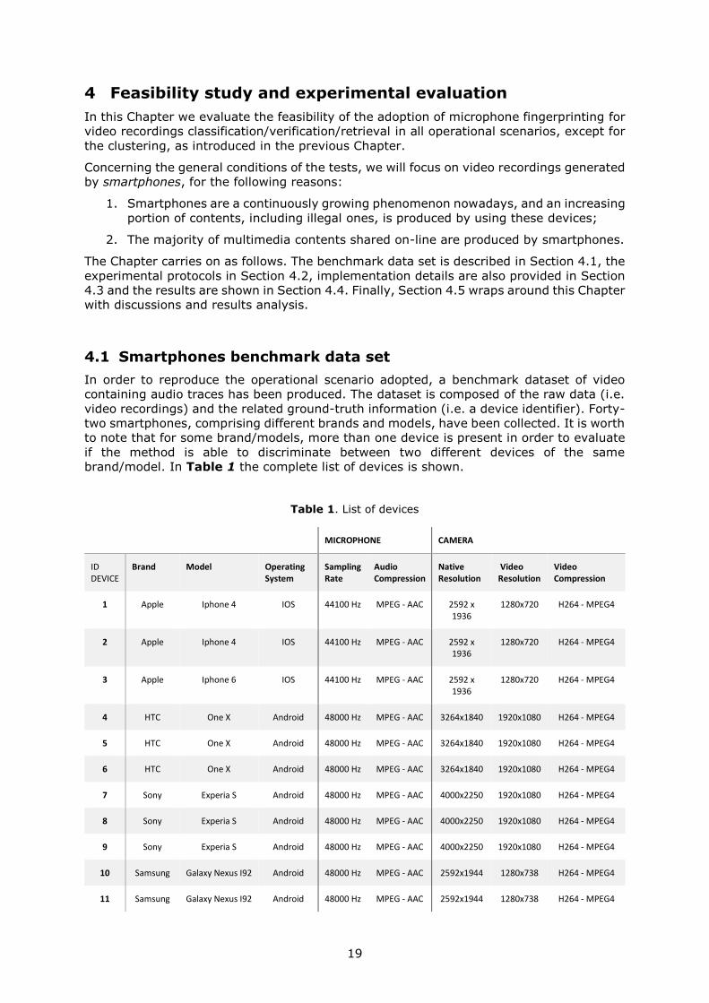
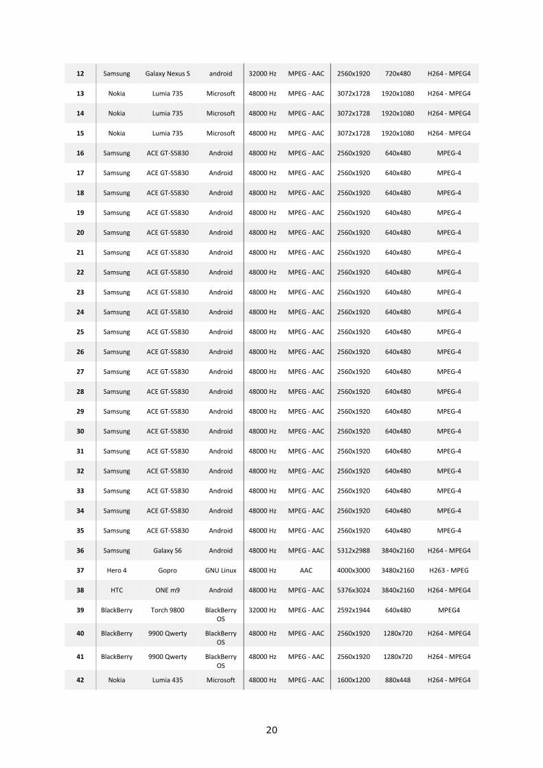
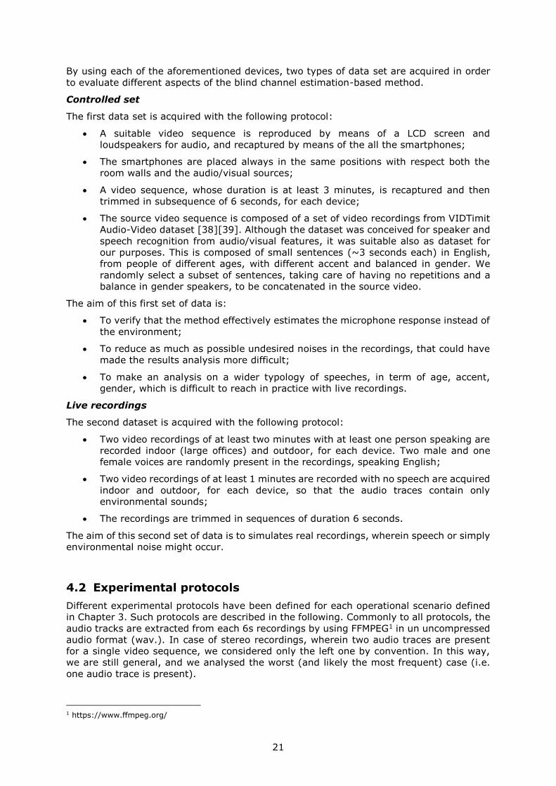
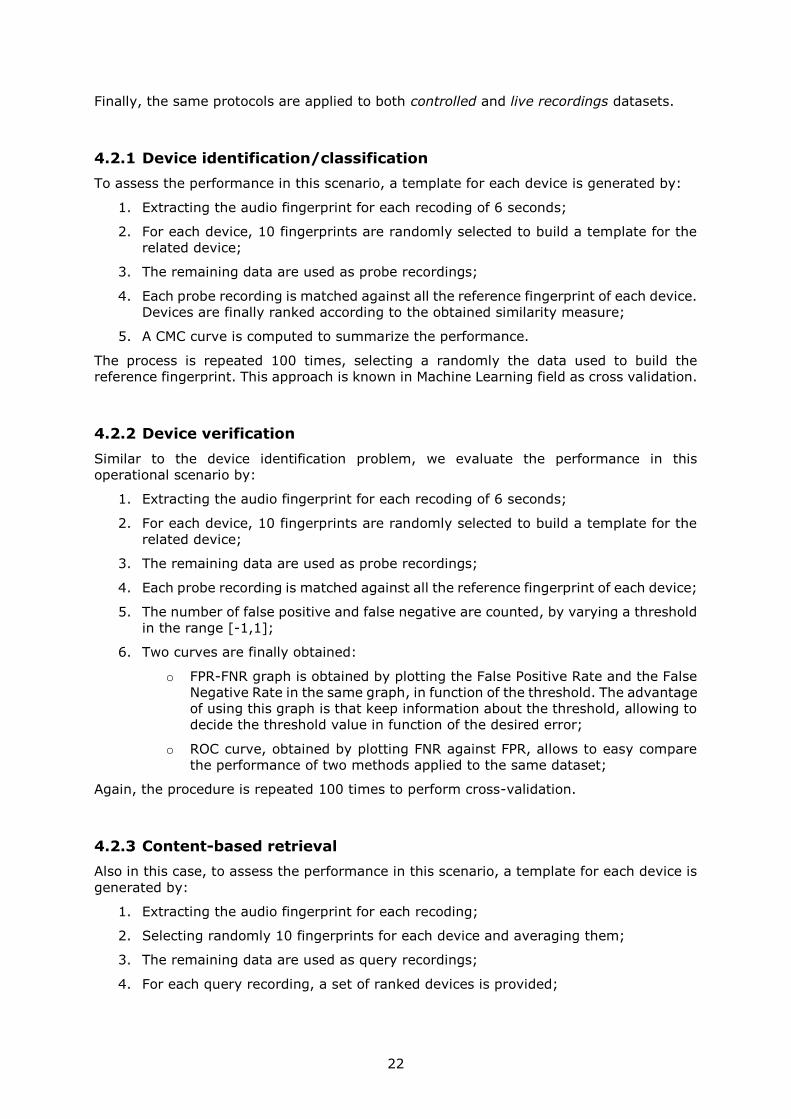
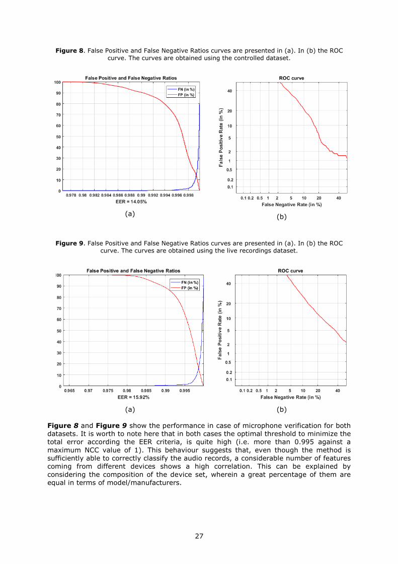
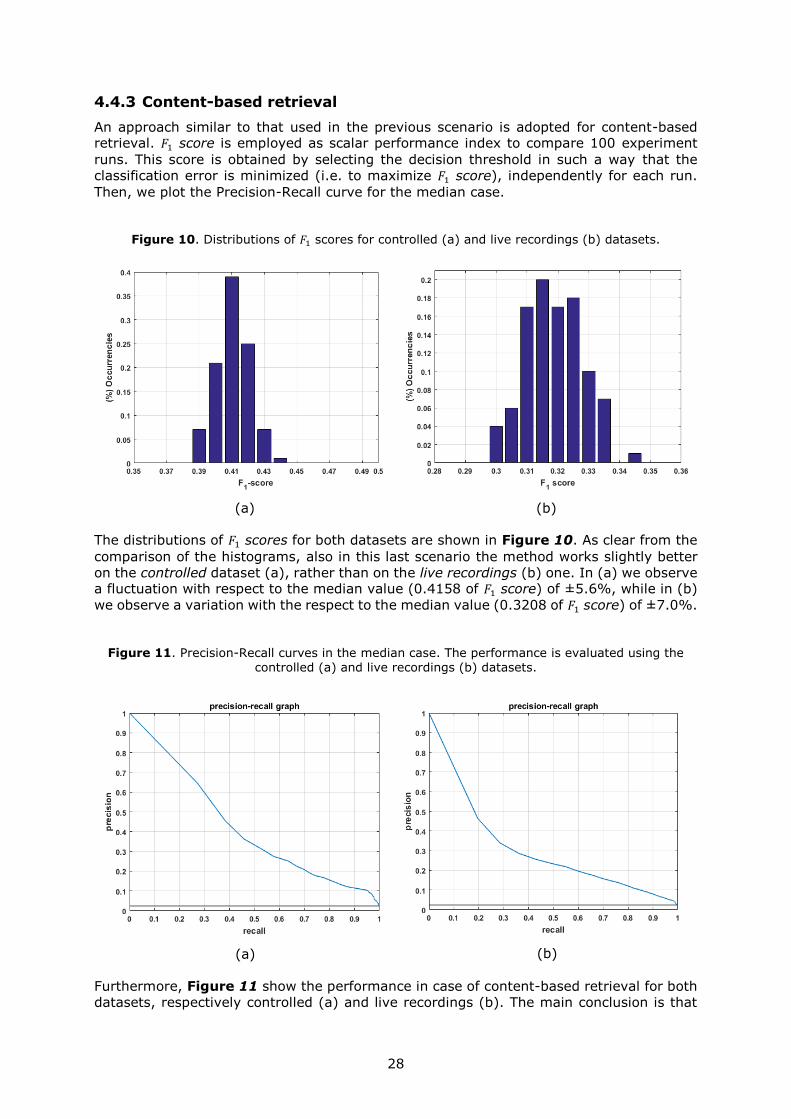
28







(a)

(b)






(a)

(b)



29























independently


speech data





median value


experiment runs

Probes

Speech Non-speech

Tem

pla



30








significantly





Probes

Speech Non-speech

Tem

pla










Probes

Speech Non-speech

Tem

pla







31















32

5 Conclusions









fingerprinting


needs



method






























33





54 Future works




level







techniques







desirable




strategies


on the field



34

References



Centre 2015





ID 496701 22 pages 2013






2015




63-74 2007




56 2009



152011












Sciences 22(3)754-767 2014



Kong 2014 pp 586-591

35











1051-2004 2017







NY USA 441-452 2014






1051-2004 2014
















36


























2006






1977



pp 199-208 2009



2004 2004



37
















NN Neural Network



















38

List of figures













28



39

List of tables









30



runs 30



Freephone number ()


charge you)



Free publications

bull one copy






Priced publications


KJ-N

A-29197

-EN

-N

doi102760775442

ISBN 978-92-79-81850-9

29























independently


speech data





median value


experiment runs

Probes

Speech Non-speech

Tem

pla



30








significantly





Probes

Speech Non-speech

Tem

pla










Probes

Speech Non-speech

Tem

pla







31















32

5 Conclusions









fingerprinting


needs



method






























33





54 Future works




level







techniques







desirable




strategies


on the field



34

References



Centre 2015





ID 496701 22 pages 2013






2015




63-74 2007




56 2009



152011












Sciences 22(3)754-767 2014



Kong 2014 pp 586-591

35











1051-2004 2017







NY USA 441-452 2014






1051-2004 2014
















36


























2006






1977



pp 199-208 2009



2004 2004



37
















NN Neural Network



















38

List of figures













28



39

List of tables









30



runs 30



Freephone number ()


charge you)



Free publications

bull one copy






Priced publications


KJ-N

A-29197

-EN

-N

doi102760775442

ISBN 978-92-79-81850-9

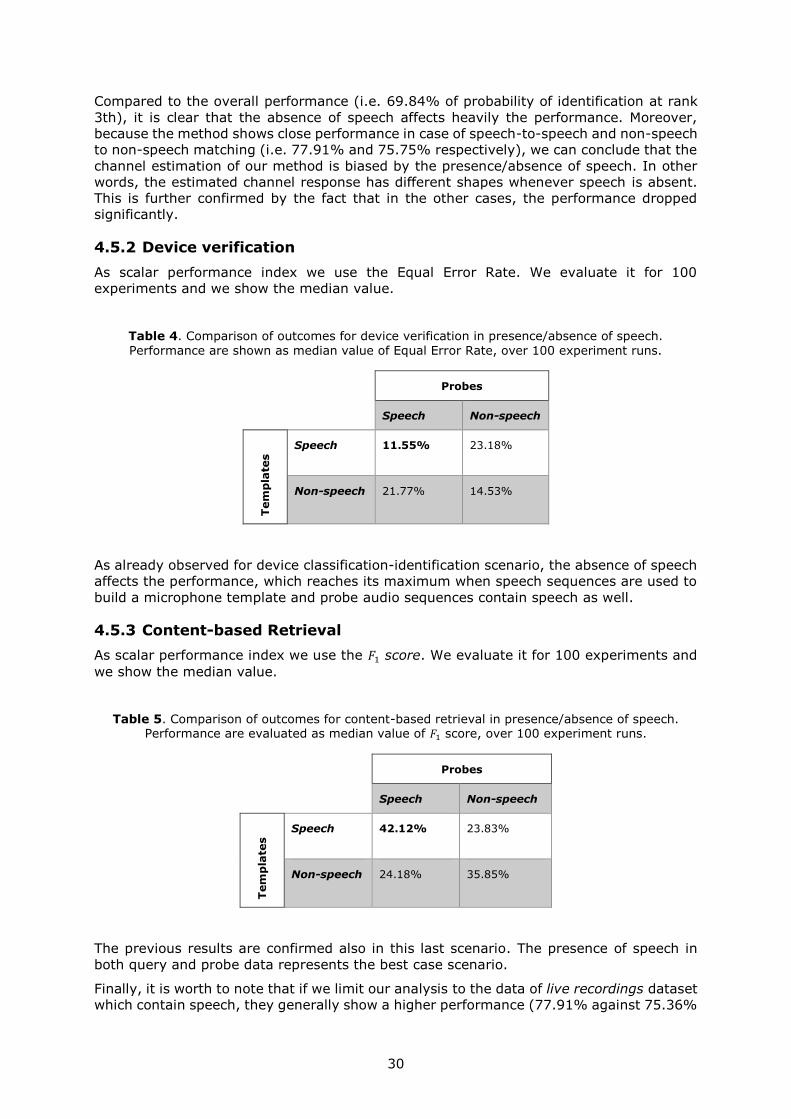
30








significantly





Probes

Speech Non-speech

Tem

pla










Probes

Speech Non-speech

Tem

pla







31















32

5 Conclusions









fingerprinting


needs



method






























33





54 Future works




level







techniques







desirable




strategies


on the field



34

References



Centre 2015





ID 496701 22 pages 2013






2015




63-74 2007




56 2009



152011












Sciences 22(3)754-767 2014



Kong 2014 pp 586-591

35











1051-2004 2017







NY USA 441-452 2014






1051-2004 2014
















36


























2006






1977



pp 199-208 2009



2004 2004



37
















NN Neural Network



















38

List of figures













28



39

List of tables









30



runs 30



Freephone number ()


charge you)



Free publications

bull one copy






Priced publications


KJ-N

A-29197

-EN

-N

doi102760775442

ISBN 978-92-79-81850-9

31















32

5 Conclusions









fingerprinting


needs



method






























33





54 Future works




level







techniques







desirable




strategies


on the field



34

References



Centre 2015





ID 496701 22 pages 2013






2015




63-74 2007




56 2009



152011












Sciences 22(3)754-767 2014



Kong 2014 pp 586-591

35











1051-2004 2017







NY USA 441-452 2014






1051-2004 2014
















36


























2006






1977



pp 199-208 2009



2004 2004



37
















NN Neural Network



















38

List of figures













28



39

List of tables









30



runs 30



Freephone number ()


charge you)



Free publications

bull one copy






Priced publications


KJ-N

A-29197

-EN

-N

doi102760775442

ISBN 978-92-79-81850-9

32

5 Conclusions









fingerprinting


needs



method






























33





54 Future works




level







techniques







desirable




strategies


on the field



34

References



Centre 2015





ID 496701 22 pages 2013






2015




63-74 2007




56 2009



152011












Sciences 22(3)754-767 2014



Kong 2014 pp 586-591

35











1051-2004 2017







NY USA 441-452 2014






1051-2004 2014
















36


























2006






1977



pp 199-208 2009



2004 2004



37
















NN Neural Network



















38

List of figures













28



39

List of tables









30



runs 30



Freephone number ()


charge you)



Free publications

bull one copy






Priced publications


KJ-N

A-29197

-EN

-N

doi102760775442

ISBN 978-92-79-81850-9

33





54 Future works




level







techniques







desirable




strategies


on the field



34

References



Centre 2015





ID 496701 22 pages 2013






2015




63-74 2007




56 2009



152011












Sciences 22(3)754-767 2014



Kong 2014 pp 586-591

35











1051-2004 2017







NY USA 441-452 2014






1051-2004 2014
















36


























2006






1977



pp 199-208 2009



2004 2004



37
















NN Neural Network



















38

List of figures













28



39

List of tables









30



runs 30



Freephone number ()


charge you)



Free publications

bull one copy






Priced publications


KJ-N

A-29197

-EN

-N

doi102760775442

ISBN 978-92-79-81850-9

34

References



Centre 2015





ID 496701 22 pages 2013






2015




63-74 2007




56 2009



152011












Sciences 22(3)754-767 2014



Kong 2014 pp 586-591

35











1051-2004 2017







NY USA 441-452 2014






1051-2004 2014
















36


























2006






1977



pp 199-208 2009



2004 2004



37
















NN Neural Network



















38

List of figures













28



39

List of tables









30



runs 30



Freephone number ()


charge you)



Free publications

bull one copy






Priced publications


KJ-N

A-29197

-EN

-N

doi102760775442

ISBN 978-92-79-81850-9

35











1051-2004 2017







NY USA 441-452 2014






1051-2004 2014
















36


























2006






1977



pp 199-208 2009



2004 2004



37
















NN Neural Network



















38

List of figures













28



39

List of tables









30



runs 30



Freephone number ()


charge you)



Free publications

bull one copy






Priced publications


KJ-N

A-29197

-EN

-N

doi102760775442

ISBN 978-92-79-81850-9

36


























2006






1977



pp 199-208 2009



2004 2004



37
















NN Neural Network



















38

List of figures













28



39

List of tables









30



runs 30



Freephone number ()


charge you)



Free publications

bull one copy






Priced publications


KJ-N

A-29197

-EN

-N

doi102760775442

ISBN 978-92-79-81850-9

37
















NN Neural Network



















38

List of figures













28



39

List of tables









30



runs 30



Freephone number ()


charge you)



Free publications

bull one copy






Priced publications


KJ-N

A-29197

-EN

-N

doi102760775442

ISBN 978-92-79-81850-9

38

List of figures













28



39

List of tables









30



runs 30



Freephone number ()


charge you)



Free publications

bull one copy






Priced publications


KJ-N

A-29197

-EN

-N

doi102760775442

ISBN 978-92-79-81850-9

39

List of tables









30



runs 30



Freephone number ()


charge you)



Free publications

bull one copy






Priced publications


KJ-N

A-29197

-EN

-N

doi102760775442

ISBN 978-92-79-81850-9



Freephone number ()


charge you)



Free publications

bull one copy






Priced publications


KJ-N

A-29197

-EN

-N

doi102760775442

ISBN 978-92-79-81850-9

KJ-N

A-29197

-EN

-N

doi102760775442

ISBN 978-92-79-81850-9

microphone smart device fingerprinting from video recordings

Documents