School of Environmental Sciences - ENV University of East Anglia - UEA

Conservation prioritisation of South Australian marine biodiversity:

Effectiveness and efficiency of the protected areas network

A dissertation presented in part-fulfilment of the degree of Master of Science in Applied Ecology and Conservation, in accordance with the regulations of the University of East Anglia. Supervision of Dr Aldina Franco (UEA) and co-supervision of Dr Bronwyn Gillanders and Dr Bertram Ostendorf (University of Adelaide – UofA).

Rebecca Borges e Silva August - 2013

School of Biological Sciences University of East Anglia Norwich Research Park Norwich NR4 7TJ

@2013 Rebecca Borges e Silva This copy of the dissertation has been supplied on condition that anyone who consults it is understood to recognize

that its copyright rests with the author and that no quotation from the dissertation, nor any information derived

there from, may be published without the author’s prior written consent. Moreover, it is supplied on the

understanding that it represents an internal University document and that neither the University nor the author are

responsible for the factual or interpretive correctness of the dissertation.

Borges, R. 2013

2

ABSTRACT

In the marine environment, protected areas represent a strategy to reduce biodiversity loss.

However, non-systematic design often leads to reserves that do not contribute to biodiversity

representativeness. This study aimed to evaluate the effectiveness and efficiency of the new

South Australian marine parks system through 1) a biodiversity coverage analysis that

compares zones with different levels of protection; and 2) an administrative units analysis that

assesses efficiency in the representation of species and habitats obtained from designs at the

state and at the regional scales. An expansion of the no-take zones to 10% of the study area was

also investigated. The outer boundaries of South Australian marine protected areas provide

good coverage of biodiversity (mean = 66.59%, se = 3.543), but only a small amount of the

distribution of species and habitats are preserved in no-take zones (mean = 13.82%, se = 2.053),

while some features are completely excluded from these higher protection level zones. The

administrative units analysis showed no considerable decrease in efficiency when priorities are

set at the regional scale, although, at this design scale, solutions present concentrated proposed

reserves near the borders of the bioregions – edge artefacts. However, for the expansion of the

no-take zones to 10% of the State waters, efficiency is considerably reduced in the regional

approach, but without enhanced edge artefacts. For the 10%-expansion scenario, comparing

and combining different solutions might be preferred to spread out new no-take zones and

consequently reduce the social conflicts that these new areas could cause.

Key-words: marine protected areas – spatial planning – gap analysis – administrative units –

edge artefacts

Borges, R. 2013

3

TABLE OF CONTENTS

ACKNOWLEDGEMENTS_________________________________________________________________________________4

1. INTRODUCTION_______________________________________________________________________________________6

1.1 Global marine biodiversity conservation 6

1.2 Marine conservation in South Australia 7

1.3 Project aims and relevance for conservation 8

2. METHODS______________________________________________________________________________________________9

2.1 Study area 9

2.2 Software 9

2.3 Source and processing of datasets 12

2.4 Effectiveness: gap analysis 13

2.5 Statistical analysis 14

2.6 Efficiency: administrative units analysis 14

2.7 Expansion of the no-take zones 15

3. RESULTS______________________________________________________________________________________________16

3.1 Effectiveness: gap analysis 16

3.2 Efficiency: administrative units analysis 21

3.3 Expansion of the no-take zones 25

4. DISCUSSION__________________________________________________________________________________________29

4.1 Gap analysis and expansion of no-take zones 29

4.2 Administrative units analysis 31

5. CONCLUSIONS_______________________________________________________________________________________34

6. CONSERVATION IMPLICATIONS _________________________________________________________________35

7. REFERENCES________________________________________________________________________________________37

I. APPENDIX A__________________________________________________________________________________________41

II. APPENDIX B_________________________________________________________________________________________42

III. APPENDIX C________________________________________________________________________________________45

IV. APPENDIX D________________________________________________________________________________________46

Borges, R. 2013

4

ACKNOWLEDGEMENTS

I thank my supervisors Dr Aldina Franco, Dr Bronwyn Gillanders and Dr Bertram

Ostendorf for the academic and technical support to deal with conservation concerns and with a

range of pieces of software that are supposed to help answer these issues, but that also raise

others ecological questions in the process.

Many thanks also to the European Commission and its Education, Audiovisual and

Culture Executive Agency (EACEA) for the Erasmus Mundus scholarship, and to the European

Master in Applied Ecology (EMAE) coordinators and secretaries Yves Caubet, Mark Hassall,

Wilhelm Windhorst, Martin Zimmer, Paulo Sousa, Mathieu Siccard, Sophie Levesque, Freddie-

Jeanne Richard and Simon Allen.

I am grateful to the South Australian Department of Environment, Water and Natural

Resources (DEWNR) for kindly providing all the spatial layers used in this study. My special

thanks to Rosemary Paxinos and Alison Wright, for explaining details of the marine parks design

process in South Australia and giving ideas for the study.

Luckily, I was surrounded by ArcGIS specialists: many thanks also to professor Andrew

Lovett and my EMAE-mate Abdullah Nagy, for extra support with the software. Many thanks

also to our full-time EMAE statistics advisor Pamela Castañeda. For all the help with maps,

directions and interactions, I am so grateful to Juliana Pille Arnold, my official research partner,

with all her experience in daytime excursions and especially nocturnal field trips. I also thank

Maria Fernanda Tirado for expert assistance in ArcGIS, Zonation, and isolation; Edgar Bracho for

the political and philosophical advice, and Samy Bracho, for important help in understanding

foreign and unknown languages.

I thank my family and friends who are not around but somehow always supported me,

even though most of them have absolutely no idea what this work is all about. Two of them,

though, were really present despite being so far away: Muito, muito obrigada Aline Andrade e

Paula Aragão pelas conversas que me salvaram tantas vezes. For the ones that are around and

understand what I’m doing, each one of you had a special part in this experience and

consequently in this work.

Borges, R. 2013

5

“And forget not that the earth delights to feel your bare feet and the winds long to play with your hair.”

Kahlil Gibran

Borges, R. 2013

6

1. INTRODUCTION

1.1 Global marine biodiversity conservation

Human societies depend on services and goods provided by ecosystems (MEA, 2003). In

the marine environment, fish populations, for instance, provide food and employment on which

livelihoods depend, besides regulatory and provisional functions that benefit the ecosystems

(Holmlund and Hammer, 1999). Fish stocks as a resource have been collapsing at ever higher

rates, causing the decline of stability, water quality and recovery potential of seas and oceans.

Biodiversity loss is impairing the capacity of marine ecosystems to provide food, maintain water

quality, and recover from perturbations (Worm et al., 2006). These declining trends are still

reversible, and marine protected areas (MPAs) have been shown, for example, to help recover

species richness, which consequently leads to increases in fisheries productivity (Worm et al.,

2006; Worm et al., 2009; Vandeperre et al., 2011).

Protected areas play a role in in situ biodiversity conservation, and their management

effectiveness serves as a valid and measurable indicator of the achievement of conservation

goals (Chape et al., 2005). However, non-systematic design has led to the selection of protected

areas that do not contribute to biodiversity representativeness. The effectiveness of the

solutions aimed to meet conservation targets should therefore be reviewed, so that political

decisions can be taken to improve the representativeness and persistence of protected areas

(Margules and Pressey, 2000).

Random MPA designs yield less benefits compared to an optimized spatial management,

even when the same total area is protected (Rassweiler et al., 2012). The complementarity

approach, which is incorporated in reserve selection algorithms for systematic planning, is

more efficient than simple selection criteria (such as buying available intact land), even when

considering the biodiversity inventory costs. Governments and organizations should, therefore,

invest in high quality surveys before establishing protected areas networks (Balmford and

Gaston, 1999).

Borges, R. 2013

7

1.2 Marine conservation in South Australia

South Australian State waters hold one of the highest levels of marine endemism in

Australia (Edyvane, 1999), with 90-95% of its known species either endemic or of restricted

range. Its marine ecosystems are considered to have national and global conservation

significance due to the fact that 75% of the red algae, 85% of the fish species and 95% of the sea

grasses are endemic to the southern regions. However, with more than 90% of South

Australians living on or near the coast, biodiversity has suffered from increased human pressure

on the marine habitats. The local government has identified pollution, bioinvasion and

environmental destruction as the main threats in the region and has pointed to considerable

habitat losses in coastal wetlands, dune systems, reefs and seagrass communities (Government

of South Australia, 2004).

In order to help safeguard marine biodiversity within its coastal waters, the South

Australian government has recently expanded the marine parks system (DEH, 2009). However,

even though it comprises about 46% of the coastal waters, the final network still leaves out

some of South Australian biodiversity (Conservation Council SA, 2013). This might be especially

relevant for the most threatened sub-regions or for the no-take zones inside the parks, since

these zones make up only 6% of the State waters. The astonishingly large size of the network

might mislead the general public’s impression that biodiversity is being effectively protected

and result in what Agardy et al. (2011) called a “dangerous illusion of protection”.

Furthermore, reserve solutions were originally designed at the regional level taking into

consideration targets that reflected conservation priorities specific to each of the eight South

Australian marine bioregions (DEH, 2009). However, local-scale designs are less efficient in

representing biodiversity when compared to a more global approach (Strange et al., 2006;

Vasquez et al., 2008; Bladt et al., 2009).

Borges, R. 2013

8

1.3 Project aims and relevance for conservation

This study aimed to evaluate effectiveness and efficiency of the South Australian marine

parks system in representing marine biodiversity through 1) a gap analysis that compares no-

take and lower-protection zones (effectiveness); and 2) an administrative units analysis that

assesses the representation of biodiversity by state- versus bioregion-scale designs (design scale

efficiency). Moreover, a third aim of this study is to propose an expansion of the no-take areas

using different design methods, through which efficiency is once more analysed.

Such a combination of problem identification and proposal of alternative solutions is a

much-needed applied approach to the establishment of protected areas, and this case study

raises methodological issues that might help better understand and therefore improve spatial

planning in various conservation contexts.

Borges, R. 2013

9

2. METHODS

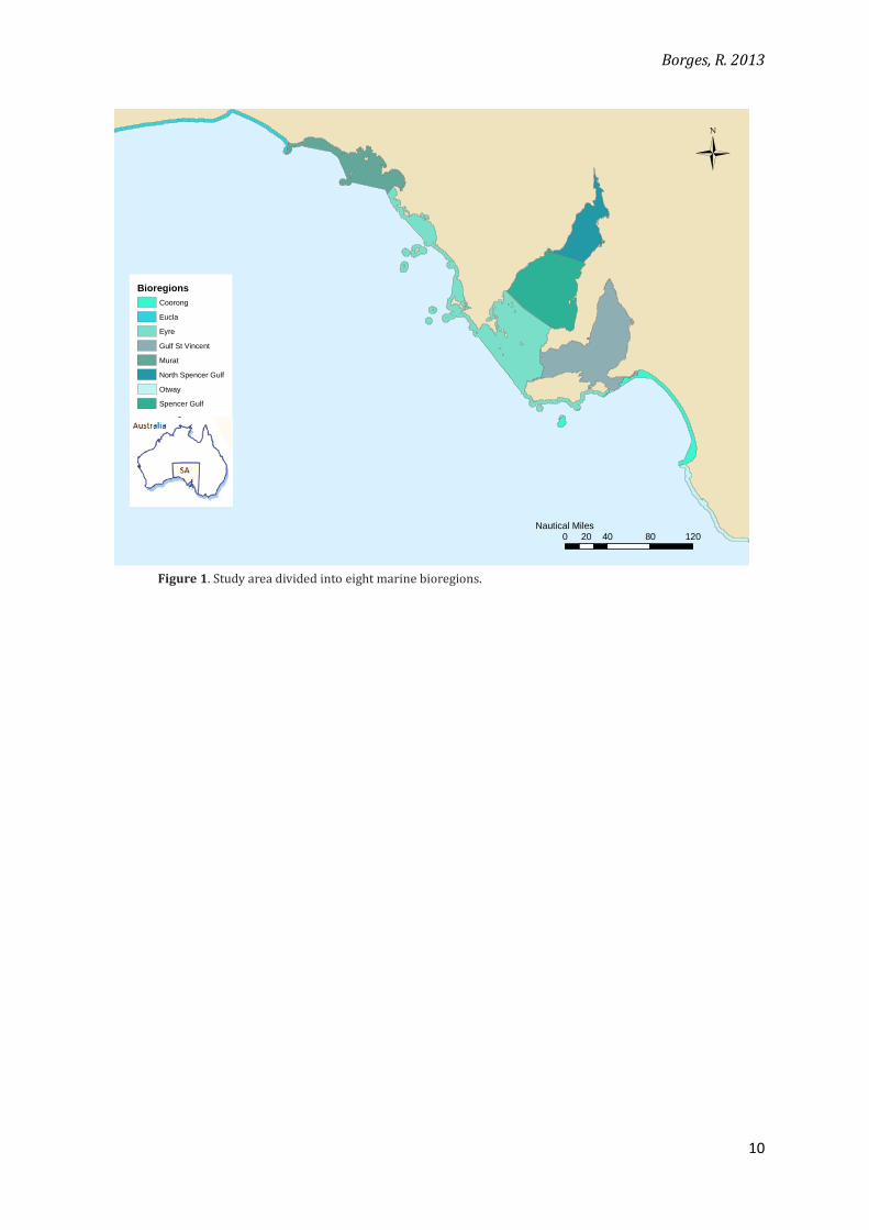
2.1 Study area

The study area comprises South Australian State waters: all estuarine and marine waters

from the highest tide to 3 nm out to sea including all bays and gulfs (Interim Marine and Coastal

Regionalisation Technical Group, 2008). Coastal waters cover an area of 60,282 km2 and 5,716

km of coastline. However, only the areas of the eight South Australian marine bioregions (Day et

al., 2008) inside coastal waters were considered; offshore islands were excluded from this study

(Figure 1).

2.2 Software

Reserve selection algorithms are mathematical tools that facilitate the spatial design of

protected areas by indicating which parts of the landscape have the highest conservation values,

according to the amount and type of biodiversity that they hold. Some of the main principles

that have been recently incorporated into these tools are 1) complementarity: selected sites

should complement each other so that the biodiversity they hold together meets defined targets;

and 2) connectivity: reserve selection favours sites in the landscape that are spatially connected,

which therefore reduces the total perimeter of the network of sites and minimises edge effects.

Borges, R. 2013

10

Figure 1. Study area divided into eight marine bioregions.

Bioregions

Coorong

Eucla

Eyre

Gulf St Vincent

Murat

North Spencer Gulf

Otway

Spencer Gulf

0 40 80 12020Nautical Miles

Ü

Borges, R. 2013

11

The publicly available software Zonation produces, through iterative cell removal, a

nested sequence of highly connected landscape structures, showing core areas of biodiversity

distribution and buffer zones of removed cells around them (Moilanen, 2007). The method used

here was Core Area Zonation, which yields a performance curve that plots the areas remaining

in the landscape versus the mean distribution of biodiversity features (species and habitats)

held inside these remaining areas. Core Area Zonation was chosen because it increases the

coverage of range-restricted features that occur in low-diversity regions (Moilanen et al., 2012)

and balances the protection granted to the fauna species considered here, which have very

small distribution relative to the other features.

The other algorithm used is Marxan, along with its graphical user interface Zonae Cogito

(Segan et al., 2011). Marxan deals with the “minimum set problem” and aims to design a reserve

system that achieves biodiversity representation targets for the smallest possible cost (Ball and

Possingham, 2000). This software uses an objective function that combines the cost of the

system and a penalty for not meeting targets for the conservation features, and it might also

consider a measure of fragmentation, through the user-defined parameter BLM – Boundary

Length Modifier- and a cost threshold penalty. A penalty for not achieving targets might also be

inserted in the design process, the Conservation Feature Penalty Factor – CFPF. The lower the

final value of the object function, the better the reserve system.

∑

∑

∑

Concerning the reserve design process, Marxan and Core Area Zonation differ in that

targets for Marxan are set for each biodiversity feature, and, in this study, a minimum cost to

achieve those targets is presented in terms of total size of the reserve system. Zonation, on the

other hand, shows a gradient in the study area that reflects the removal order of cells based on

Borges, R. 2013

12

their conservation value. Therefore, targets for Zonation are taken as the percentage of the area

remaining in the landscape, and the software presents how much of the distribution of

biodiversity features is retained at each stage of the cell removal process.

Zonation also has a reserve design tool based on administrative units, in which the eight

marine bioregions can be analysed together, with only a few easily-created extra input files. For

a similar approach, Marxan would require separate analyses, with individually-built input files,

a much more time-consuming approach.

The software ArcGIS Desktop 10.1 was used for the gap analysis, while the package SPSS

version 18 was used to perform the statistical tests.

2.3 Source and processing of datasets

The data used for all three analyses correspond to a sub-set of the spatial layers with the

distributions of species and habitats used by the South Australian Department of Environment,

Water and Natural Resources (DEWNR) to select the areas for the creation of the current

marine parks network at the initial stages of the selection process. Layers with the location of

the marine parks and the delimitation of the State waters and its bioregions were also provided

by DEWNR. Concerning resolution, the marine benthic habitats were mapped at a 1:100,000

scale. However, metadata in general were scarcely available.

The layers were independently formatted to meet requirements for Marxan, and then

further formatted for Zonation. Among the large dataset provided, the initial layers selected

were those with the best levels of certainty and resolution (avoiding, for example, labels such as

“likely to be present”). Other redundant layers were either merged with the primarily selected

ones or excluded from the analysis. (For further information on data limitation, refer to

Appendix A.)

Initial processing of GIS layers consisted of creating small buffers around data-points

(just so their area could be calculated – a requirement for Marxan) and spatially limiting all

features to the study area. For the Marxan analysis, the area was divided into 17,014 planning

Borges, R. 2013

13

cells with varying sizes of up to 4km2 (the ones at the edge were smaller), and the area of the

distribution of biodiversity features and protected areas inside each cell was tabulated. The final

processing of the tabulated areas and the creation of a list of features used in Marxan input files

was done using the interface Zonae Cogito. Other required input files were generated using

ArcGIS and Excel spreadsheets.

For Zonation, independent grid cells of 1km2 that fall completely inside the study area

were used and separately inserted into the software. Zonation, contrary to Marxan, requires that

all cells have the same size. Therefore, the total area for the two sets of analyses is not exactly

the same. Furthermore, the number of conservation features used as inputs for both pieces of

software was also slightly different (157 for Marxan and 151 for Zonation), because the layer

preparation procedure for Marxan is more sensitive to small-range features (For a complete list

of the biodiversity features used, refer to Appendix B). Thus, comparison between the solutions

proposed by the two packages is limited.

2.4 Effectiveness: gap analysis

A gap analysis consists of combining conservation features’ distributions (such as

species ranges) and maps of protected areas to show how well biodiversity is represented in the

existing network of reserves (Jennings, 2000; Rodrigues et al., 2004).

This part of the analysis, therefore, aims to assess the proportion of the distribution of

each biodiversity feature in the study area held by the marine protected areas. The approach

was applied to the entire South Australian coastal waters and to two individual bioregions: 1)

North Spencer Gulf, which presents high levels of endemism, especially in species that usually

occur in tropical ecosystems; and 2) Spencer Gulf, which, chosen due to high diversity and

productivity, supports important recreational and commercial fisheries (DEH, 2009).

This measure of effectiveness was done in regards to the protection level of the zones

inside the parks. Using the software ArcGIS Desktop 10.0, the area of the selected conservation

Borges, R. 2013

14

features was calculated: 1) inside the no-take zones; and 2) inside the remaining, lower-

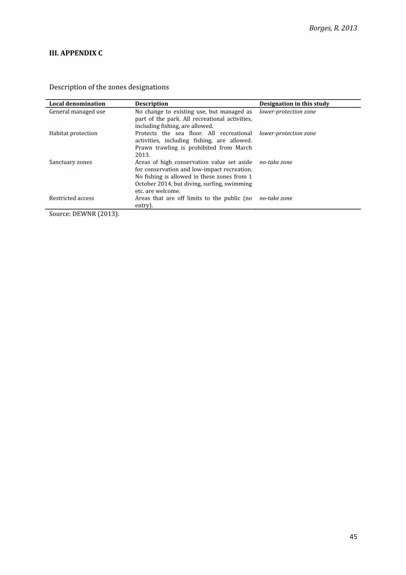
protection zones. For the present study, the denomination “no-take zone” refers to the locally-

assigned Sanctuary Zones and Restricted Access Zones, which actually still allow “low-impact

fishing” (DEWNR, 2013). These areas could roughly be placed in the categories I to III from the

protected areas classification created by the International Union for Conservation of Nature

(IUCN). (For a more-detailed clarification of the zones designations used in this study, refer to

Appendix C).

2.5 Statistical analysis

A paired-sample t-test (t) was used to compare the total area of the distribution of

biodiversity features covered by no-takes zones with the expected distribution that would be

covered based solely on the size of these zones (random selection of MPAs). The square root of

the areas was used to perform the test. A Wilcoxon signed rank test (Z) was used to compare the

total area of the distributions of biodiversity features inside no-takes zones with the area

covered by the other lower-protection zones.

2.6 Efficiency: administrative units analysis

The aim of this analysis is to test if more biodiversity is supported in a system designed

at the bioregional or at the state scales. Using Zonation, the planning scales for reserve selection

were compared based on performance (species distribution coverage over different proportions

of the landscape being protected), for the 46%-area target, which corresponds to the extension

of the entire network.

To reduce the total network perimeter, a range of Boundary Length Penalty (BLP) values

were visually inspected and the parameter was then set to 1. Other general parameters were

kept as default. Specific parameters for the administrative units analysis followed similar

methodology to Moilanen and Arponen (2011): beta A = 0.999 and q = 0.001.

For the administrative units analysis, five scenarios were compared:

Borges, R. 2013

15

1) the state scale planning (mode 0);

2) a regional scale planning (mode 2) using South Australian eight marine bioregions:

2a) with equal weights applied to the bioregions and 2b) with weights proportional to the size

of each bioregion; and

3) a regional scale planning (mode 2) using eight randomly-created administrative units:

3a) with equal weights applied to the units and 3b) with weights proportional to the size of each

unit.

2.7 Expansion of the no-take zones

As a more practical approach to conservation management, an expansion of total size of

the no-take zones is proposed using two different pieces of software: Zonation and Marxan. In

the case of Zonation, the expansion occurs preferably inside the network, but is proposed as well

outside. The CBD-10%-area target was chosen for the expansion. The state and bioregional

planning scales were again examined in terms of efficiency for the expansion scenario, to check

how these results compare with those from the administrative units analysis.

The Marxan design, on the other hand, was set to only allow the expansion of the no-take

zones inside the system. Moreover, targets are defined per biodiversity feature. However, setting

a 10%-area target should yield a best solution that covers about 10% of South Australian coastal

waters, due to the fact that some features considered here are spread-out through the whole of

the study area. Marxan allows for easy identification of the conservation features for which the

10% could not be met inside the current marine parks system. Boundary Length Modifier - BLM

and Conservation Feature Penalty Factor – CFPF were calibrated to 1000 and 1, respectively, and

the software was set to propose 1000 solutions for the design problem. Here, reserve design is

done only at the state scale.

Borges, R. 2013

16

3. RESULTS

3.1 Effectiveness: gap analysis

The current South Australian network provides good coverage of biodiversity (mean =

66.59%, se = 3.543), but representation showed considerable variation among the different

species and habitats: some are well-represented while others have very little of their

distributions protected (Figures 2 and 3). Coverage of the distribution of features in no-take

zones is significantly smaller than that inside the lower-protection-level zones (Wilcoxon signed

rank test Z = -5.214, df = 38, p < 0.001, N = 39) (Figure 4). Furthermore, the proportion of

species and habitats in no-take zones is not significantly different from a random design

(paired-sample t-test t = 0.869, df = 38, p = 0.390, N = 39).

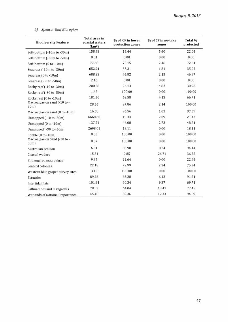
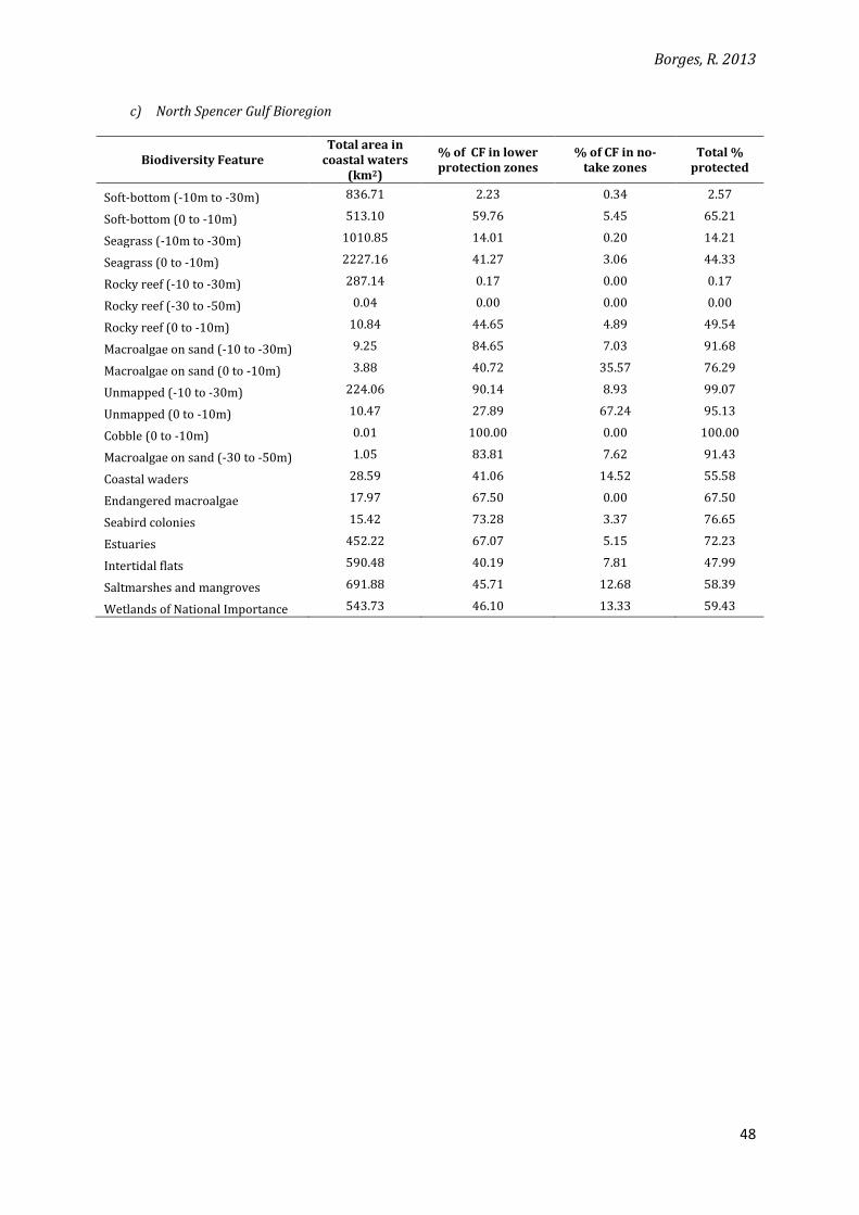
The same pattern is observed for both the Spencer Gulf and the North Spencer Gulf

bioregions (Figure 4). Coverage for each feature in no-take zones is significantly smaller than

that inside the other zones (Spencer Gulf: Wilcoxon signed rank test Z = -4.045, df = 24, p <

0.001; North Spencer Gulf: Z = -3.622, df = 19, p < 0.001). Coverage for each feature in no-take

zones is not significantly different from what would be expected based solely on the size of

these zones in comparison to the networks in each of these bioregions (Spencer Gulf: t = -0.510,

df = 24, p = 0.614, N = 25; North Spencer Gulf: t = 0.991; df = 19; p = 0.334, N = 20). Moreover,

the proportion of no-take zones inside the marine parks is slightly larger than for the whole of

the State waters: 7% of the total bioregion area for Spencer Gulf and 9% for North Spencer Gulf.

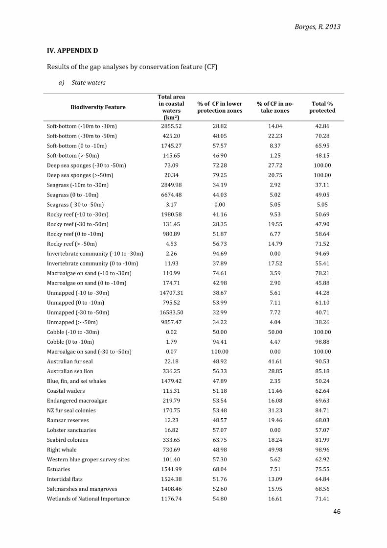
(For a detailed description of the proportions of biodiversity features inside the different types

of zones, refer to Appendix D.)

In terms of number of species, the class Aves seems to be well-represented in all zones

at the State waters level. Classes Mammalia and Reptilia, however, follow the general pattern of

low-coverage in no-take zones (Figure 5).

Borges, R. 2013

17

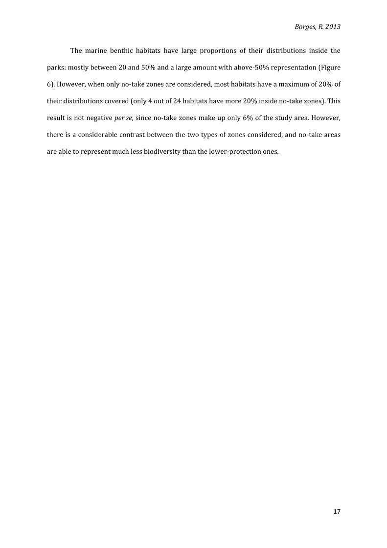
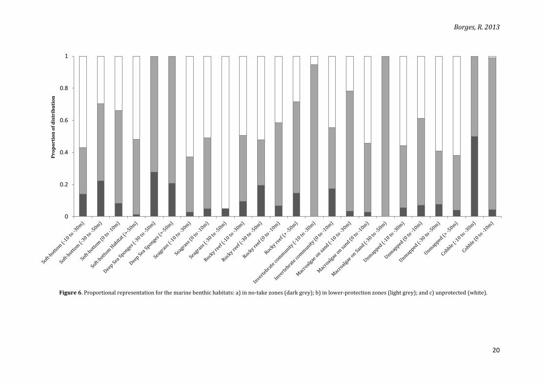
The marine benthic habitats have large proportions of their distributions inside the

parks: mostly between 20 and 50% and a large amount with above-50% representation (Figure

6). However, when only no-take zones are considered, most habitats have a maximum of 20% of

their distributions covered (only 4 out of 24 habitats have more 20% inside no-take zones). This

result is not negative per se, since no-take zones make up only 6% of the study area. However,

there is a considerable contrast between the two types of zones considered, and no-take areas

are able to represent much less biodiversity than the lower-protection ones.

Borges, R. 2013

18

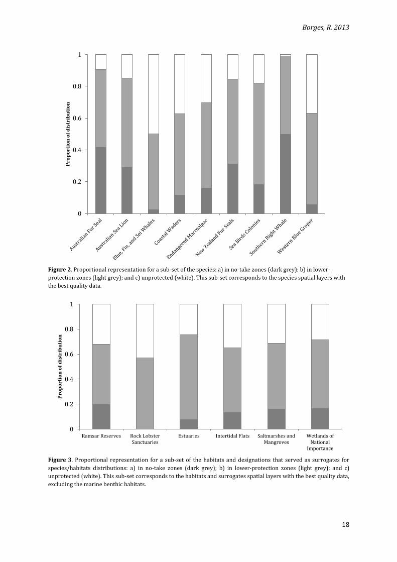
Figure 2. Proportional representation for a sub-set of the species: a) in no-take zones (dark grey); b) in lower-

protection zones (light grey); and c) unprotected (white). This sub-set corresponds to the species spatial layers with

the best quality data.

Figure 3. Proportional representation for a sub-set of the habitats and designations that served as surrogates for

species/habitats distributions: a) in no-take zones (dark grey); b) in lower-protection zones (light grey); and c)

unprotected (white). This sub-set corresponds to the habitats and surrogates spatial layers with the best quality data,

excluding the marine benthic habitats.

0

0.2

0.4

0.6

0.8

1

Ramsar Reserves Rock LobsterSanctuaries

Estuaries Intertidal Flats Saltmarshes andMangroves

Wetlands ofNational

Importance

Pro

po

rtio

n o

f d

istr

ibu

tio

n

0

0.2

0.4

0.6

0.8

1

Pro

po

rtio

n o

f d

istr

ibu

tio

n

Borges, R. 2013

19

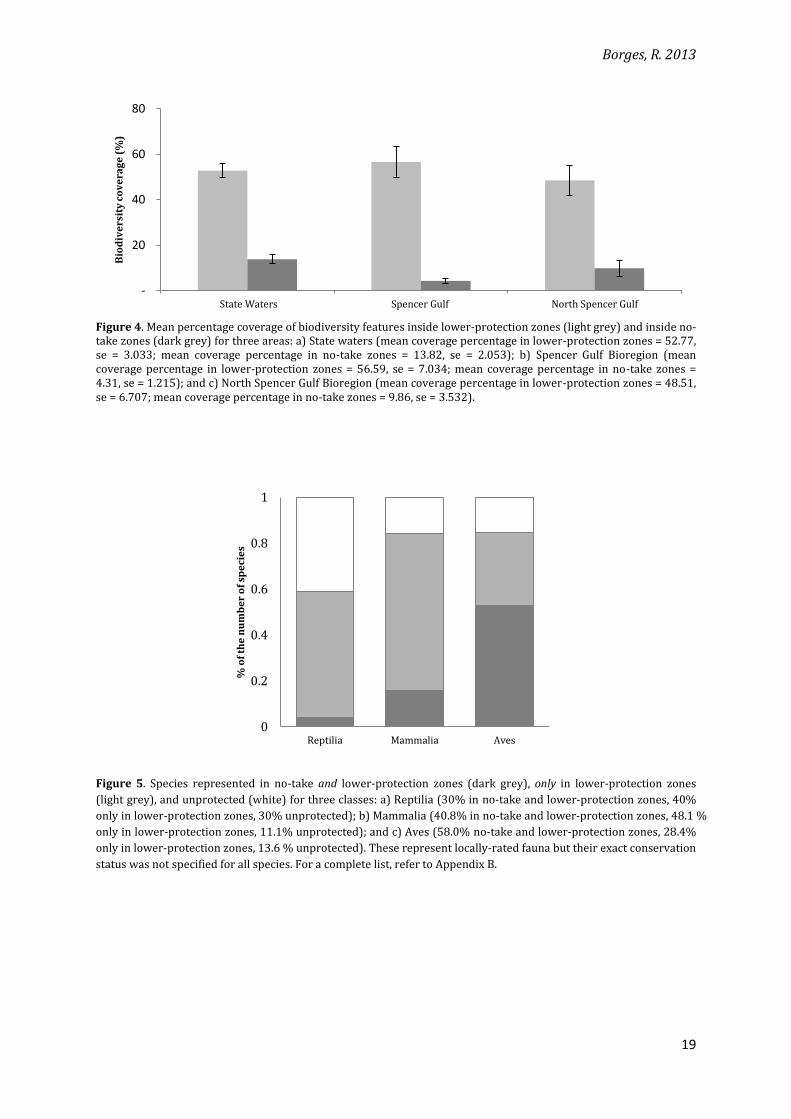
Figure 4. Mean percentage coverage of biodiversity features inside lower-protection zones (light grey) and inside no-take zones (dark grey) for three areas: a) State waters (mean coverage percentage in lower-protection zones = 52.77, se = 3.033; mean coverage percentage in no-take zones = 13.82, se = 2.053); b) Spencer Gulf Bioregion (mean coverage percentage in lower-protection zones = 56.59, se = 7.034; mean coverage percentage in no-take zones = 4.31, se = 1.215); and c) North Spencer Gulf Bioregion (mean coverage percentage in lower-protection zones = 48.51, se = 6.707; mean coverage percentage in no-take zones = 9.86, se = 3.532).

Figure 5. Species represented in no-take and lower-protection zones (dark grey), only in lower-protection zones

(light grey), and unprotected (white) for three classes: a) Reptilia (30% in no-take and lower-protection zones, 40%

only in lower-protection zones, 30% unprotected); b) Mammalia (40.8% in no-take and lower-protection zones, 48.1 %

only in lower-protection zones, 11.1% unprotected); and c) Aves (58.0% no-take and lower-protection zones, 28.4%

only in lower-protection zones, 13.6 % unprotected). These represent locally-rated fauna but their exact conservation

status was not specified for all species. For a complete list, refer to Appendix B.

-

20

40

60

80

State Waters Spencer Gulf North Spencer Gulf

Bio

div

ers

ity

co

ve

rag

e (

%)

0

0.2

0.4

0.6

0.8

1

Reptilia Mammalia Aves

% o

f th

e n

um

be

r o

f sp

eci

es

Borges, R. 2013

20

Figure 6. Proportional representation for the marine benthic habitats: a) in no-take zones (dark grey); b) in lower-protection zones (light grey); and c) unprotected (white).

0

0.2

0.4

0.6

0.8

1P

rop

ort

ion

of

dis

trib

uti

on

21

3.2 Efficiency: administrative units analysis

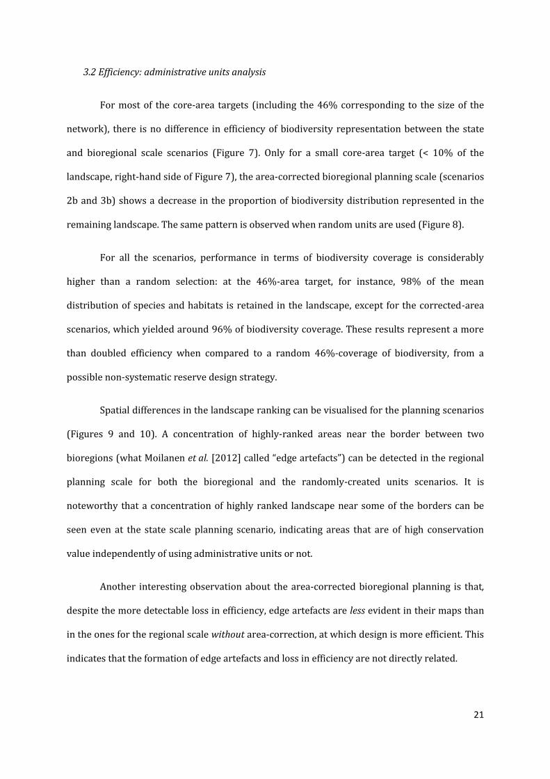
For most of the core-area targets (including the 46% corresponding to the size of the

network), there is no difference in efficiency of biodiversity representation between the state

and bioregional scale scenarios (Figure 7). Only for a small core-area target (< 10% of the

landscape, right-hand side of Figure 7), the area-corrected bioregional planning scale (scenarios

2b and 3b) shows a decrease in the proportion of biodiversity distribution represented in the

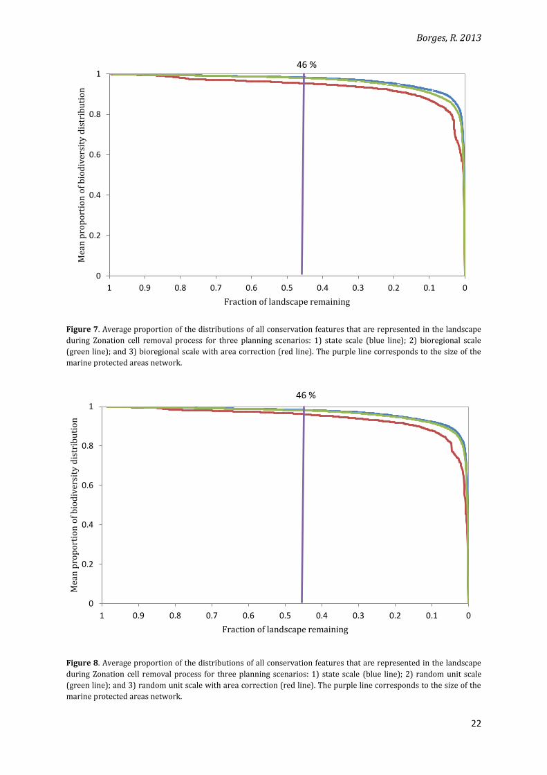
remaining landscape. The same pattern is observed when random units are used (Figure 8).

For all the scenarios, performance in terms of biodiversity coverage is considerably

higher than a random selection: at the 46%-area target, for instance, 98% of the mean

distribution of species and habitats is retained in the landscape, except for the corrected-area

scenarios, which yielded around 96% of biodiversity coverage. These results represent a more

than doubled efficiency when compared to a random 46%-coverage of biodiversity, from a

possible non-systematic reserve design strategy.

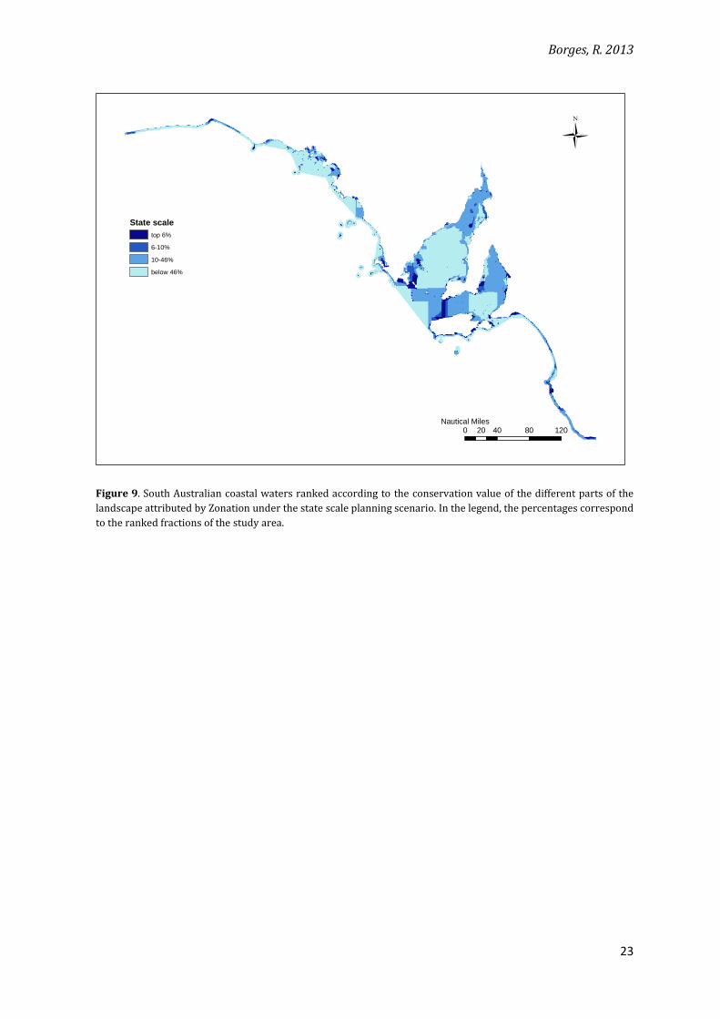
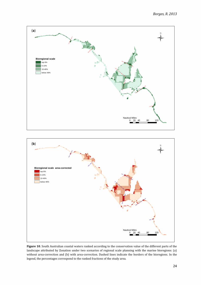
Spatial differences in the landscape ranking can be visualised for the planning scenarios

(Figures 9 and 10). A concentration of highly-ranked areas near the border between two

bioregions (what Moilanen et al. [2012] called “edge artefacts”) can be detected in the regional

planning scale for both the bioregional and the randomly-created units scenarios. It is

noteworthy that a concentration of highly ranked landscape near some of the borders can be

seen even at the state scale planning scenario, indicating areas that are of high conservation

value independently of using administrative units or not.

Another interesting observation about the area-corrected bioregional planning is that,

despite the more detectable loss in efficiency, edge artefacts are less evident in their maps than

in the ones for the regional scale without area-correction, at which design is more efficient. This

indicates that the formation of edge artefacts and loss in efficiency are not directly related.

Borges, R. 2013

22

Figure 7. Average proportion of the distributions of all conservation features that are represented in the landscape

during Zonation cell removal process for three planning scenarios: 1) state scale (blue line); 2) bioregional scale

(green line); and 3) bioregional scale with area correction (red line). The purple line corresponds to the size of the

marine protected areas network.

Figure 8. Average proportion of the distributions of all conservation features that are represented in the landscape

during Zonation cell removal process for three planning scenarios: 1) state scale (blue line); 2) random unit scale

(green line); and 3) random unit scale with area correction (red line). The purple line corresponds to the size of the

marine protected areas network.

0

0.2

0.4

0.6

0.8

1

00.10.20.30.40.50.60.70.80.91

Mea

n p

rop

ort

ion

of

bio

div

ersi

ty d

istr

ibu

tio

n

Fraction of landscape remaining

46 %

0

0.2

0.4

0.6

0.8

1

00.10.20.30.40.50.60.70.80.91

Mea

n p

rop

ort

ion

of

bio

div

ersi

ty d

istr

ibu

tio

n

Fraction of landscape remaining

46 %

Borges, R. 2013

23

Figure 9. South Australian coastal waters ranked according to the conservation value of the different parts of the

landscape attributed by Zonation under the state scale planning scenario. In the legend, the percentages correspond

to the ranked fractions of the study area.

State scale

top 6%

6-10%

10-46%

below 46%

Ü

0 40 80 12020Nautical Miles

Borges, R. 2013

24

Figure 10. South Australian coastal waters ranked according to the conservation value of the different parts of the

landscape attributed by Zonation under two scenarios of regional scale planning with the marine bioregions: (a)

without area-correction and (b) with area-correction. Dashed lines indicate the borders of the bioregions. In the

legend, the percentages correspond to the ranked fractions of the study area.

Ü

0 40 80 12020Nautical Miles

Bioregional scale

top 6%

6-10%

10-46%

below 46%

Ü

0 40 80 12020Nautical Miles

Bioregional scale area-corrected

top 6%

6-10%

10-46%

below 46%

(a)

(b)

Borges, R. 2013

25

3.3 Expansion of the no-take zones

3.3.1 Zonation

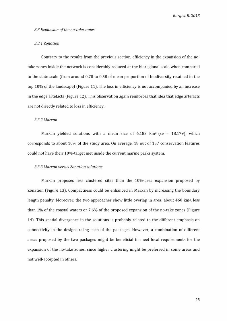
Contrary to the results from the previous section, efficiency in the expansion of the no-

take zones inside the network is considerably reduced at the bioregional scale when compared

to the state scale (from around 0.78 to 0.58 of mean proportion of biodiversity retained in the

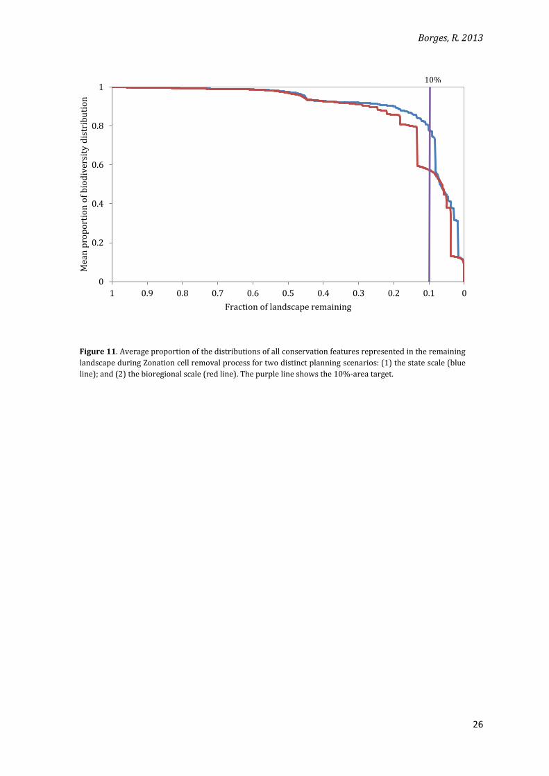
top 10% of the landscape) (Figure 11). The loss in efficiency is not accompanied by an increase

in the edge artefacts (Figure 12). This observation again reinforces that idea that edge artefacts

are not directly related to loss in efficiency.

3.3.2 Marxan

Marxan yielded solutions with a mean size of 6,183 km2 (se = 18.179), which

corresponds to about 10% of the study area. On average, 18 out of 157 conservation features

could not have their 10%-target met inside the current marine parks system.

3.3.3 Marxan versus Zonation solutions

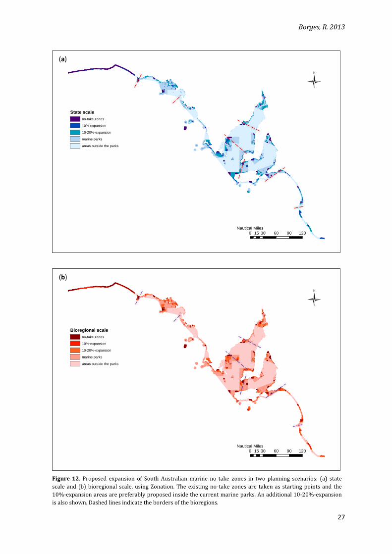
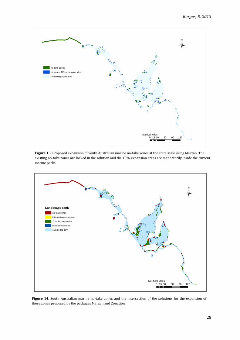
Marxan proposes less clustered sites than the 10%-area expansion proposed by

Zonation (Figure 13). Compactness could be enhanced in Marxan by increasing the boundary

length penalty. Moreover, the two approaches show little overlap in area: about 460 km2, less

than 1% of the coastal waters or 7.6% of the proposed expansion of the no-take zones (Figure

14). This spatial divergence in the solutions is probably related to the different emphasis on

connectivity in the designs using each of the packages. However, a combination of different

areas proposed by the two packages might be beneficial to meet local requirements for the

expansion of the no-take zones, since higher clustering might be preferred in some areas and

not well-accepted in others.

Borges, R. 2013

26

Figure 11. Average proportion of the distributions of all conservation features represented in the remaining

landscape during Zonation cell removal process for two distinct planning scenarios: (1) the state scale (blue

line); and (2) the bioregional scale (red line). The purple line shows the 10%-area target.

0

0.2

0.4

0.6

0.8

1

00.10.20.30.40.50.60.70.80.91

Mea

n p

rop

ort

ion

of

bio

div

ersi

ty d

istr

ibu

tio

n

Fraction of landscape remaining

10%

Borges, R. 2013

27

Figure 12. Proposed expansion of South Australian marine no-take zones in two planning scenarios: (a) state

scale and (b) bioregional scale, using Zonation. The existing no-take zones are taken as starting points and the

10%-expansion areas are preferably proposed inside the current marine parks. An additional 10-20%-expansion

is also shown. Dashed lines indicate the borders of the bioregions.

Ü

0 30 60 90 12015Nautical Miles

State scale

no-take zones

10%-expansion

10-20%-expansion

marine parks

areas outside the parks

Ü

0 30 60 90 12015Nautical Miles

Bioregional scale

no-take zones

10%-expansion

10-20%-expansion

marine parks

areas outside the parks

(a)

(b)

Borges, R. 2013

28

Figure 13. Proposed expansion of South Australian marine no-take zones at the state scale using Marxan. The

existing no-take zones are locked in the solution and the 10%-expansion areas are mandatorily inside the current

marine parks.

Figure 14. South Australian marine no-take zones and the intersection of the solutions for the expansion of

these zones proposed by the packages Marxan and Zonation.

0 30 60 90 12015Nautical Miles

Ü

no-take zones

proposed 10%-extension sites

remaining study area

ÜLandscape rank

no-take zones

intersection expansion

Zonation expansion

Marxan expansion

outside top 10%

0 30 60 90 12015

Nautical Miles

Borges, R. 2013

29

3. DISCUSSION

4. 1 Gap analysis and expansion of no-take zones

The South Australian marine parks network supports a relatively good average

proportion of the distribution of the conservation features analysed (mean = 66.59%, se =

3.543).

Other studies evaluating the present representativeness of protected areas in the

marine environment, especially comparing different protection categories, are rarely found in

the peer-reviewed literature. There may be some evaluations in the “grey literature”, such as

technical reports, but these are often difficult to access. It is difficult, therefore, to compare the

present assessment to the performance of MPAs in other regions.

Comparisons can be drawn with global compilations and a recent national evaluation of

the Australia MPAs. For example, having 46% of State waters covered by parks in South

Australia is well above the global proportion of 1.4% of protected coastal shelves (Chape et al.,

2005), and it corresponds to a representation level that is even higher than the 36% for the

MPAs in Australian commonwealth waters (not including State waters) (Barr and Possingham,

2013).

On the other hand, no-take zones are ineffective in representing many features; some

species and habitats have very little of their distributions covered or none at all. Out of the 24

marine benthic habitats analysed, for instance, 14 have less than 10% for their distribution

covered, while 2 are not included at all in no-take zones. In terms of total area reserved, South

Australian no-take zones do worse than the national MPAs network, which covers 13% of

Australian jurisdiction waters (Barr and Possingham, 2013).

Benefits to biodiversity attributed to the establishment of MPAs, such as increased

density, depend on the level of protection in marine reserves. Examples in the recent literature

either point to better results of no-take areas when compared to lower-protection categories

Borges, R. 2013

30

(e.g., Scott et al., 2012; Lester and Halpern, 2008) or solely refer to positive impacts specifically

from no-take areas (e.g., Gormley et al., 2013; Rassweiler et al., 2012).

Therefore, an increase in South Australian no-take areas would be necessary to cover

the distributions of gap or poorly-represented features. The Great Barrier Reef MPA in Australia,

for instance, now has 33% of its area included in no-take zones (Fernandes et al., 2005). The

expansion of South Australian no-take areas would reduce the protection gap between the

different zones and re-assure the commitment of the State in effectively protecting its marine

biodiversity.

But socio-political challenges to this expansion clearly exist in South Australia. Some of the

population living near the established no-take zones have already expressed dissatisfaction, and

many fear that the ban to recreational fisheries will reduce the number of tourists and affect

local economies (Novak, 2012). On the other hand, fisheries can benefit from spillover of adults

and larvae from no-take areas (Lester et al., 2009). Therefore, a geographical balance of no-take

and fishing areas could increase catches and provide benefits to local communities in the long-

run, provided these no-take zones are systematic designed.

Moreover, Lester et al. (2009) in their global synthesis concluded that reserve size does

not influence performance and even small MPAs can increase average size of organisms.

Therefore, the expansion of the higher-protection-level zones could be done through the

creation of new no-take areas far from the existing ones, so other fishing zones could benefit

from spill-over. Spreading out no-take zones across the landscape could also avoid

concentrating social conflicts and overloading certain local communities with large areas of

restricted-access zones. However, the fact that these zones are often surrounded by the others

inside large parks could be an advantage if a buffer-like expansion was chosen in some areas, as

proposed by Zonation for certain parts of the landscape. Many small no-take areas also may

have additional costs in terms of ensuring enforcement.

Borges, R. 2013

31

Depending on specific targets for the expansion, the use of Zonation or Marxan, or even

a combination of their outputs would be beneficial. If connectivity is preferred for certain areas,

Zonation is a better approach, while a Marxan-based solution might be more suitable to spread-

out expansion sites while keeping a minimised cost. The spatial solutions presented here,

however, are illustrative of these possible scenarios, and new expansion exercises should be

done with a more complete dataset, which would include social-economic variables, especially

data on recreational and commercial fisheries. It may also be useful to have additional

information on connectivity of key organisms, for example, dispersal distances and pathways.

4.2 Administrative units analysis

The visual comparison between the scenarios from planning at different scales show a

divergence in terms of areas assigned as the most valuable for conservation, and edge artefacts

can be detected in the bioregion-level scenarios. However, overall network efficiency was only

minimally reduced for a reserve design based on strong emphasis on local conservation

priorities when compared to state-scale representation (Figures 7 and 8).

These results are contrary to previous studies (Vasquez et al., 2008; Bladt et al., 2009;

Kark et al., 2009), which show that coordinated solutions at larger scales tend to increase

flexibility and therefore efficiency in site selection. Setting conservation priorities at larger

scales avoid the extra cost, for example, of covering the distribution of biodiversity features that

are locally rare but more common when other geopolitical units are considered (Strange et al.,

2006), a sort of “artificial rarity” in the solution caused by the planning scale choice.

However, considering that the marine bioregions are distinctly affected by human

pressure (DEH, 2009), it is still ecologically important to assess how each one is doing in terms

of biodiversity representation. This evaluation could then serve as a proxy to how the

establishment of protected areas is distributed and to try and avoid the concentration of areas in

Borges, R. 2013

32

regions that might be considered “cheaper” for conservation because they are not of economical

interest.

Moilanen and Arponen (2011) and Moilanen et al. (2012) used a very similar software

analysis but also found some reduction in efficiency. The latter also detected edge artefacts, and

argued that these decrease the efficiency of conservation strategies. Even though edge artefacts

were detected in the present study, these are visually less intense and therefore may not

directly cause a loss in efficiency. Edge artefacts might only reflect a re-allocation of the areas

considered by Zonation to have the highest conservation values, but not necessarily imply that

overall more areas have to be reserved so that similar proportions of biodiversity are

represented. Spatial planning procedures should ideally check for these artefacts and analyse

how this re-allocation affects the design solutions in order to decide whether these effects

should be avoided or not in the planning process.

The similarity in the results for both the bioregions and the random units indicate that,

even though bioregions were established on ecological criteria, they do not necessarily

represent areas that contain most of a certain species’ or a habitat’s distribution. This would

make these features be considered rare when present in other regions and possibly cause

differences in efficiency for both scenarios. However, it can be speculated that a higher number

of smaller units would increase the artificial-rarity phenomenon and decrease the efficiency of

the planning design.

Nevertheless, a considerable loss in efficiency was observed in the expansion of the no-

take zones inside the current system. The features’ distributions that were previously larger in

the whole of the coastal waters become medium-sized when selection is favoured inside marine

parks, which therefore allows for an enhanced artificial or scale-related rarity. The emphasis on

regional conservation priorities assigns rarity to biodiversity features in the regions that might

not have been considered rare at the state scale priority setting. As reported in the previously-

mentioned papers, this requires more area to be preserved in the bioregional scenario so that

Borges, R. 2013

33

the same mean proportion of biodiversity is overall represented, since more species and

habitats are now being recognised by the software as rare.

But again this extra area is not necessarily located in areas where MPAs are crossed by

the border between two bioregions. Edge artefacts were not increased at the bioregional scale

in the expansion scenario, when compared to the scenarios that did not consider the MPAs,

despite the considerable loss of efficiency at the 10%-area target. Even though edge artefacts

have been reported to reduce the efficiency of the spatial design process (Moilanen et al., 2012),

this loss might be attributed to extra area demanded to cover a similar proportion of

biodiversity in other areas apart from the borders of the bioregions/units.

Therefore, the different effects of the design-scale choice, whether they cause edge

artefacts, or reduce efficiency, are largely dependent on 1) spatial characteristics of biodiversity

features’ distributions; 2) the study area, whether it is continuous or segregated (as in the

expansion scenario, which favoured selection inside the current MPAs); and 3) on specific

conservation goals, since considerable differences may only be found for a restricted interval of

area-targets.

Borges, R. 2013

34

4. CONCLUSIONS

i. At the state level, South Australian marine parks effectively cover the

distributions of most of the biodiversity analysed. The Spencer Gulf and North

Spencer Gulf bioregions have similar patterns of biodiversity representation as

that for the whole of the coastal waters. However, biodiversity representation is

considered ineffective inside no-take zones, both at the state level and for those

two bioregions.

ii. The design solutions at state and bioregional scales are spatially different, but

have similar efficiency, when no pre-established parks are considered. However,

in the context of a proposed extension of no-take zones inside the current MPAs,

the bioregional-level design covers a considerably smaller proportion of

biodiversity at the 10%-area target when compared to the state-scale solution.

iii. The bioregional solutions show concentrations of high-conservation-value areas

near the borders of the bioregions (edge artefacts), but these do not seem to be

the main cause for the loss of efficiency in the planning design. The reduction in

efficiency probably depends on spatial characteristics of the distribution of the

biodiversity features included in the planning exercise, as well as specific aspects

of the study area.

iv. Marxan and Zonation yield solutions that have little spatial overlap, but similar

total area. Zonation favours the connectivity of possible extension sites, but

comparing and combining both scenarios might be preferred to spread out new

no-take zones and consequently reduce the social conflicts that these new areas

could cause.

Borges, R. 2013

35

5. CONSERVATION IMPLICATIONS

One of the aims of this study was to raise awareness and stimulate discussion on a

methodological aspect of spatial planning: the design scale. This topic had not yet been

approached for the marine environment, and specific literature for the terrestrial context is still

scarce (Vasquez et al., 2008; Bladt et al., 2009; Kark et al., 2009), with only a few studies

applying similar methodology (see Moilanen et al., 2012; Moilanen and Arponen, 2011). None of

these has considered bioregions, established on ecological criteria, as the administrative units.

Moreover, no previous work has been applied to the context of an expansion of MPAs, in which

certain parts of the study area are favoured for selection.

The inclusion of these previously-unexplored aspects of the planning process allowed

for an unprecedented discussion on the design scale, which will hopefully be carried on by

further studies, since these new aspects have important practical influence on the design of

protected areas.

As an initial step of the planning process, practitioners should examine the spatial

characteristics of the biodiversity distribution data available, bearing in mind that they might

strongly influence the final configuration and cost of the network of reserves. Secondly, spatial

characteristics of biological data might interact with the planning area and different costs for the

landscape. Certain aspects of the design solutions might depend, for example, on whether a

completely new system is being established or if an expansion of existing protected areas is

being proposed. The interaction between spatial characteristics of biodiversity distribution and

the specific planning area could then influence the solutions provided by different design scales,

even when ecological sub-units (such as the South Australian marine bioregions) are used as

planning areas. This study suggests that a larger-scale approach to spatial planning is more or at

least equally efficient and should therefore be preferred, even though loss of efficiency or edge

artefacts might actually not be verified or, when existing, these might depend on the

management targets chosen.

Borges, R. 2013

36

The use of different conservation planning packages might be advantageous to 1)

investigate how different target setting strategies influence spatial configurations, 2) assess a

variety of parameters that indicate effectiveness and efficiency of the proposed system and are

only available in either one of the packages, and 3) combine the spatial output from the different

pieces of software to reach a preferred configuration.

In the case of the South Australian marine parks, an expansion of the no-take zones to a

minimum of a 10%-area target is strongly recommended, with special emphasis on the inclusion

of gap features and the increase of the coverage of rare/endemic/threatened species and

habitats. This expansion should be conducted at the state scale and should aim also to spread

out the new no-take zones throughout the coastal waters.

However, other relevant targets and principles might strongly influence and be even

more critical for the design of the expanded no-take zones. The inclusion of fisheries

productivity as a cost metric or the decision on whether to protect highly threatened or

relatively pristine areas should also be analysed in combination with the influence of the design

scale, in order to inspect a possible trade-off between emphasis on local conservation priorities

and maximisation of efficiency in biodiversity coverage.

Borges, R. 2013

37

6. REFERENCES

Agardy T., di Sciara G.N., Christie P. (2011). Mind the gap: Addressing the shortcomings of marine

protected areas through large scale marine spatial planning. Marine Policy, 35 (2) , 226-232.

Ball, I. R. and H. P. Possingham. (2000). Marxan (v1.8.2): Marine Reserve Design Using Spatially

Explicit Annealing, a Manual.

Ball, I. R., Possingham, H. P., & Watts, M. (2009). Marxan and relatives: software for spatial

conservation prioritisation. Spatial conservation prioritisation: quantitative methods and

computational tools. Oxford University Press, Oxford, United Kingdom, 185-195.

Balmford, A., & Gaston, K.J. (1999). Why biodiversity surveys are good value. Nature, 398(6724),

204-205.

Barr, L. M., & Possingham, H. P. (2013). Are outcomes matching policy commitments in Australian

marine conservation planning?. Marine Policy, 42, 39-48.

Bladt, J., Strange, N., Abildtrup, J., Svenning, J. C., & Skov, F. (2009). Conservation efficiency of

geopolitical coordination in the EU. Journal for Nature Conservation, 17(2), 72-86.

CBD. (2006). Decisions Adopted by the Conference of the Parties to the Convention on Biological

Diversity at its Eighth Meeting (Decision VIII/15, Annex IV). Convention on Biological Diversity,

Curitiba, Brazil.

Chape, S., Harrison, J., Spalding, M., & Lysenko, I. (2005). Measuring the extent and effectiveness of

protected areas as an indicator for meeting global biodiversity targets. Philosophical Transactions

of the Royal Society B: Biological Sciences, 360(1454), 443-455.

Conservation Council SA. (2013). South Australian marine biodiversity hotspots excluded from

protection. Available at: <http://www.conservationsa.org.au/media-releases/1128-sa-marine-

biodiversity-hotspots-not-protected.html>. Access on: 29th Jan 2013.

Day, V., Paxinos, R., Emmett, J., Wright, A., & Goecker, M. (2008). The Marine Planning Framework for

South Australia: A new ecosystem-based zoning policy for marine management. Marine

Policy, 32(4), 535-543.

Department for Environment and Heritage – DEH (2009). A technical report on the outer boundaries

of South Australia’s marine parks network. Department for Environment and Heritage, South

Australia.

Borges, R. 2013

38

Department of Environment, Water and Natural Resources - DEWNR. (2013). Marine Parks - Zones

Available at: <http://www.environment.sa.gov.au/marineparks/zones>. Access on 20th June

2013.

Edyvane, K. S. (1999). Conserving marine biodiversity in South Australia–Part 2–Identification of areas

of high conservation value in South Australia. Report to Department for Environment and Heritage,

Government of South Australia, Adelaide.

Fernandes, L., Day, J. O. N., Lewis, A., Slegers, S., Kerrigan, B., Breen, D. A. N., ... & Stapleton, K. (2005).

Establishing Representative No‐Take Areas in the Great Barrier Reef: Large‐Scale

Implementation of Theory on Marine Protected Areas. Conservation Biology, 19(6), 1733-1744.

Gormley, A. M., Slooten, E., Dawson, S., Barker, R. J., Rayment, W., du Fresne, S., & Bräger, S. (2012).

First evidence that marine protected areas can work for marine mammals. Journal of Applied

Ecology, 49(2), 474-480.

Government of South Australia. Living coast strategy for South Australia. Adelaide: Natural and

Cultural Heritage, Department for Environment and Heritage; 2004.

Holmlund, C. M., & Hammer, M. (1999). Ecosystem services generated by fish populations. Ecological

Economics, 29(2), 253-268.

Interim Marine and Coastal Regionalisation Technical Group. Interim marine and coastal

regionalisation for Australia: and ecosystem-based classification for marine and coastal

environments. Version 3.3. Environment Australia, Canberra, 1998.

Jennings, M. D. (2000). Gap analysis: concepts, methods, and recent results*.Landscape

ecology, 15(1), 5-20.

Kark, S., Levin, N., Grantham, H. S., & Possingham, H. P. (2009). Between-country collaboration and

consideration of costs increase conservation planning efficiency in the Mediterranean Basin.

Proceedings of the National Academy of Sciences, 106(36), 15368-15373.

Kearney, R., Buxton, C. D., & Farebrother, G. (2012). Australia’s no-take marine protected areas:

Appropriate conservation or inappropriate management of fishing? Marine Policy, 36(5), 1064-

1071.

Kujala, H., Araújo, M. B., Thuiller, W., & Cabeza, M. (2011). Misleading results from conventional gap

analysis–Messages from the warming north. Biological Conservation, 144(10), 2450-2458.

Borges, R. 2013

39

Lester, S. E., & Halpern, B. S. (2008). Biological responses in marine no-take reserves versus partially

protected areas. Marine Ecology Progress Series, 367, 49-56.

Lester, S. E., Halpern, B. S., Grorud-Colvert, K., Lubchenco, J., Ruttenberg, B. I., Gaines, S. D., ... &

Warner, R. R. (2009). Biological effects within no-take marine reserves: a global synthesis. Marine

Ecology Progress Series, 384, 33-46.

Margules, C. R., & Pressey, R. L. (2000). Systematic conservation planning. Nature, 405(6783), 243-

253.

MEA. (2003). Millennium ecosystem assessment. Ecosystems.

Moilanen, A. (2007). Landscape zonation, benefit functions and target-based planning: unifying

reserve selection strategies. Biological Conservation, 134(4), 571-579.

Moilanen, A., Anderson, B. J., Arponen, A., Pouzols, F. M., & Thomas, C. D. (2012). Edge artefacts and

lost performance in national versus continental conservation priority areas. Diversity and

Distributions, 19(2), 171-183.

Moilanen, A., & Arponen, A. (2011). Administrative regions in conservation: balancing local priorities

with regional to global preferences in spatial planning. Biological Conservation, 144(5), 1719-

1725.

Natural Resource Management Ministerial Council (2010) Australia’s Biodiversity Conservation

Strategy 2010–2030. Australian Government, Department of Sustainability, Environment, Water,

Population and Communities, Canberra. Available at:

<http://www.environment.gov.au/biodiversity/strategy>. Access on: 31 Jan 2013.

Novak, L. (2012). Final plans for state's 19 marine parks released by SA Government. Available at:

<http://www.adelaidenow.com.au/news/south-australia/final-plans-for-states-19-marine-

parks-released-by-sa-government/story-e6frea83-1226526557652>. Access on: 8th July 2013.

Pressey, R. L., & Bottrill, M. C. (2008). Opportunism, threats, and the evolution of systematic

conservation planning. Conservation Biology, 22(5), 1340-1345.

Rassweiler, A., Costello, C., & Siegel, D. A. (2012). Marine protected areas and the value of spatially

optimized fishery management. Proceedings of the National Academy of Sciences, 109(29), 11884-

11889.

Borges, R. 2013

40

Rodrigues, A. S., Akcakaya, H. R., Andelman, S. J., Bakarr, M. I., Boitani, L., Brooks, T. M., ... & Yan, X.

(2004). Global gap analysis: priority regions for expanding the global protected-area

network. BioScience, 54(12), 1092-1100.

Scott, R., Hodgson, D. J., Witt, M. J., Coyne, M. S., Adnyana, W., Blumenthal, J. M., ... & Godley, B. J.

(2012). Global analysis of satellite tracking data shows that adult green turtles are significantly

aggregated in Marine Protected Areas. Global Ecology and Biogeography, 21(11), 1053-1061.

Segan, D. B., Game, E. T., Watts, M. E., Stewart, R. R., & Possingham, H. P. (2011). An interoperable

decision support tool for conservation planning. Environmental Modelling & Software, 26(12),

1434-1441.

Stewart, R. R., & Possingham, H. P. (2002, August). A framework for systematic marine reserve

design in South Australia: a case study. In Inaugural World Congress on Aquatic Protected Areas,

Cairns,(unpublished).

Stewart, R. R., Noyce, T., & Possingham, H. P. (2003). Opportunity cost of ad hoc marine reserve

design decisions: an example from South Australia. Marine Ecology Progress Series, 253, 25-38.

Strange, N., Thorsen, B. J., & Bladt, J. (2006). Optimal reserve selection in a dynamic world. Biological

Conservation, 131(1), 33-41.

Vandeperre, F., Higgins, R. M., Sánchez‐Meca, J., Maynou, F., Goñi, R., Martín‐Sosa, P., ... & Santos, R. S.

(2011). Effects of no‐take area size and age of marine protected areas on fisheries yields: a meta‐

analytical approach. Fish and Fisheries, 12(4), 412-426.

Vazquez, L. B., Rodríguez, P., & Arita, H. T. (2008). Conservation planning in a subdivided world.

Biodiversity and Conservation, 17(6), 1367-1377.

Worm, B., Barbier, E. B., Beaumont, N., Duffy, J. E., Folke, C., Halpern, B. S., ... & Watson, R. (2006).

Impacts of biodiversity loss on ocean ecosystem services. Science, 314(5800), 787-790.

Worm, B., Hilborn, R., Baum, J. K., Branch, T. A., Collie, J. S., Costello, C., ... & Zeller, D. (2009).

Rebuilding global fisheries. Science, 325(5940), 578-585.

Borges, R. 2013

41

I. APPENDIX A

Potential limitations of the datasets used

The accuracy of the gap analysis results is limited by independent formatting of the spatial

layers, surrogate choice, little amount of metadata available and by the fact that interactions

with other protected areas are not considered. In the case of the rock lobster, for instance, only

point-data were available. A 1-km2 buffer was then arbitrarily established around those points,

ignoring the actual area of the sanctuaries. Therefore, sanctuary areas that might overlap with

the parks network were probably ignored, and these could include also high-protection zones.

Similarly, lobster sanctuaries, which were designated under a different law, might be considered

fully no-take zones, and the matter over conflicting regulations in intersections between areas

under different laws is unclear and beyond the scope of this study. The main message is that, in

general, features might be well represented in lower-protection zones but largely excluded from

the more strict areas. Further more, the results obtained are in accordance with a local

evaluation of the network (DEH, 2009), which validates the zones comparison in this study,

even though it did not use the exact same datasets or formatting procedures.

Borges, R. 2013

42

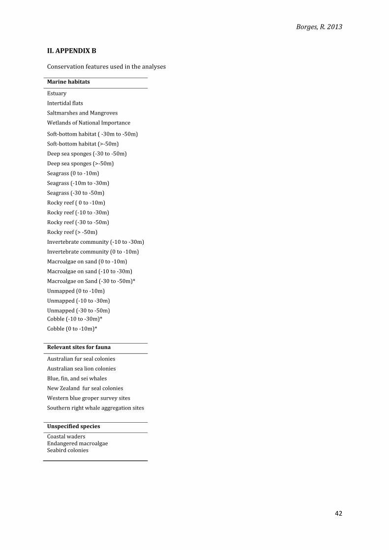
II. APPENDIX B

Conservation features used in the analyses

Marine habitats

Estuary

Intertidal flats

Saltmarshes and Mangroves

Wetlands of National Importance

Soft-bottom habitat ( -30m to -50m)

Soft-bottom habitat (>-50m)

Deep sea sponges (-30 to -50m)

Deep sea sponges (>-50m)

Seagrass (0 to -10m)

Seagrass (-10m to -30m)

Seagrass (-30 to -50m)

Rocky reef ( 0 to -10m)

Rocky reef (-10 to -30m)

Rocky reef (-30 to -50m)

Rocky reef (> -50m)

Invertebrate community (-10 to -30m)

Invertebrate community (0 to -10m)

Macroalgae on sand (0 to -10m)

Macroalgae on sand (-10 to -30m)

Macroalgae on Sand (-30 to -50m)*

Unmapped (0 to -10m)

Unmapped (-10 to -30m)

Unmapped (-30 to -50m)

Cobble (-10 to -30m)*

Cobble (0 to -10m)*

Relevant sites for fauna

Australian fur seal colonies

Australian sea lion colonies

Blue, fin, and sei whales

New Zealand fur seal colonies

Western blue groper survey sites

Southern right whale aggregation sites

Unspecified species

Coastal waders Endangered macroalgae Seabird colonies

Borges, R. 2013

43

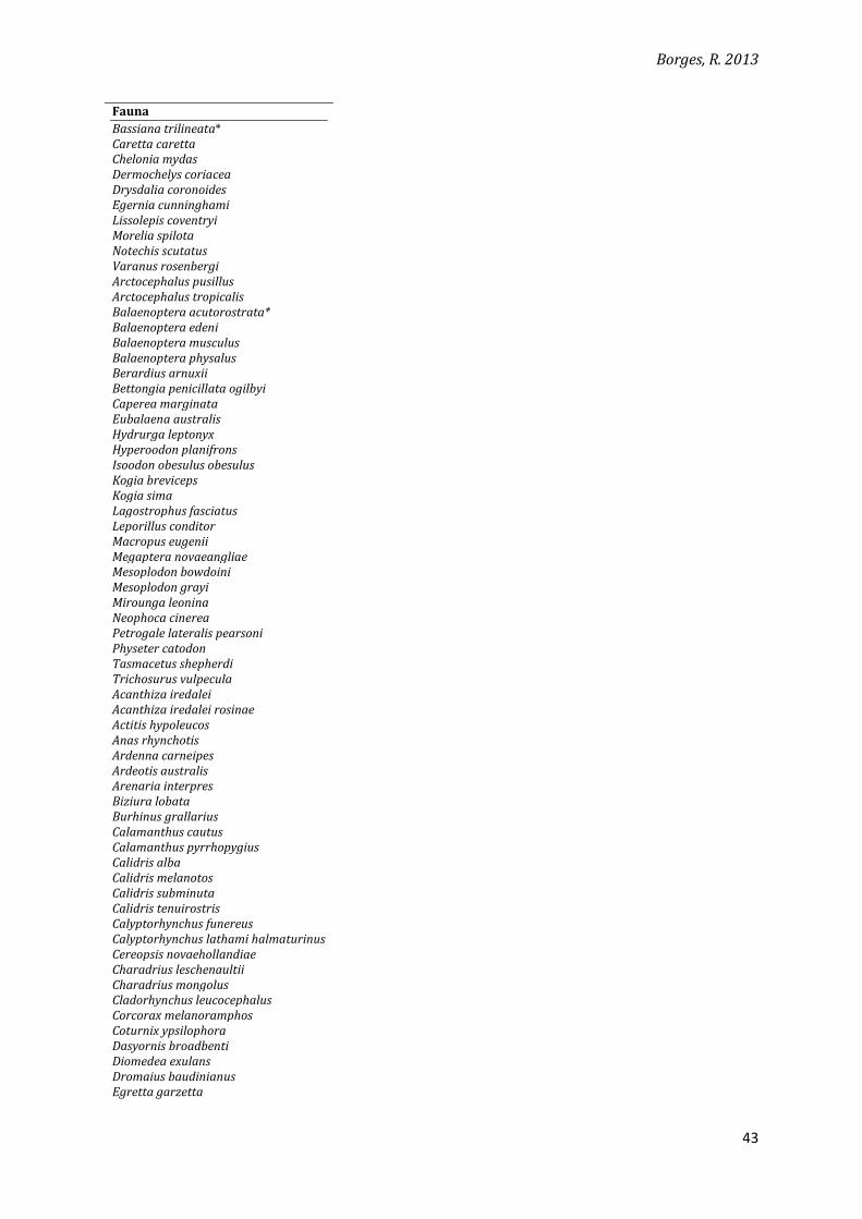
Fauna

Bassiana trilineata* Caretta caretta Chelonia mydas Dermochelys coriacea Drysdalia coronoides Egernia cunninghami Lissolepis coventryi Morelia spilota Notechis scutatus Varanus rosenbergi Arctocephalus pusillus Arctocephalus tropicalis Balaenoptera acutorostrata* Balaenoptera edeni Balaenoptera musculus Balaenoptera physalus Berardius arnuxii Bettongia penicillata ogilbyi Caperea marginata Eubalaena australis Hydrurga leptonyx Hyperoodon planifrons Isoodon obesulus obesulus Kogia breviceps Kogia sima Lagostrophus fasciatus Leporillus conditor Macropus eugenii Megaptera novaeangliae Mesoplodon bowdoini Mesoplodon grayi Mirounga leonina Neophoca cinerea Petrogale lateralis pearsoni Physeter catodon Tasmacetus shepherdi Trichosurus vulpecula Acanthiza iredalei Acanthiza iredalei rosinae Actitis hypoleucos Anas rhynchotis Ardenna carneipes Ardeotis australis Arenaria interpres Biziura lobata Burhinus grallarius Calamanthus cautus Calamanthus pyrrhopygius Calidris alba Calidris melanotos Calidris subminuta Calidris tenuirostris Calyptorhynchus funereus Calyptorhynchus lathami halmaturinus Cereopsis novaehollandiae Charadrius leschenaultii Charadrius mongolus Cladorhynchus leucocephalus Corcorax melanoramphos Coturnix ypsilophora Dasyornis broadbenti Diomedea exulans Dromaius baudinianus Egretta garzetta

Borges, R. 2013

44

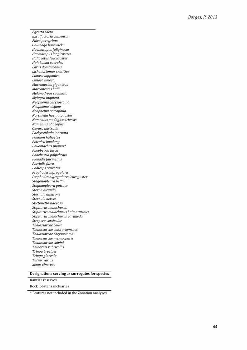
Egretta sacra Excalfactoria chinensis Falco peregrinus Gallinago hardwickii Haematopus fuliginosus Haematopus longirostris Haliaeetus leucogaster Halobaena caerulea Larus dominicanus Lichenostomus cratitius Limosa lapponica Limosa limosa Macronectes giganteus Macronectes halli Melanodryas cucullata Myiagra inquieta Neophema chrysostoma Neophema elegans Neophema petrophila Northiella haematogaster Numenius madagascariensis Numenius phaeopus Oxyura australis Pachycephala inornata Pandion haliaetus Petroica boodang Philomachus pugnax* Phoebetria fusca Phoebetria palpebrata Plegadis falcinellus Pluvialis fulva Podiceps cristatus Psophodes nigrogularis Psophodes nigrogularis leucogaster Stagonopleura bella Stagonopleura guttata Sterna hirundo Sternula albifrons Sternula nereis Stictonetta naevosa Stipiturus malachurus Stipiturus malachurus halmaturinus Stipiturus malachurus parimeda Strepera versicolor Thalassarche cauta Thalassarche chlororhynchos Thalassarche chrysostoma Thalassarche melanophris Thalassarche salvini Thinornis rubricollis Tringa brevipes Tringa glareola Turnix varius Xenus cinereus

Designations serving as surrogates for species

Ramsar reserves

Rock lobster sanctuaries

* Features not included in the Zonation analyses.

Borges, R. 2013

45

III. APPENDIX C

Description of the zones designations

Local denomination Description Designation in this study

General managed use No change to existing use, but managed as part of the park. All recreational activities, including fishing, are allowed.

lower-protection zone

Habitat protection Protects the sea floor. All recreational activities, including fishing, are allowed. Prawn trawling is prohibited from March 2013.

lower-protection zone

Sanctuary zones Areas of high conservation value set aside for conservation and low-impact recreation. No fishing is allowed in these zones from 1 October 2014, but diving, surfing, swimming etc. are welcome.

no-take zone

Restricted access Areas that are off limits to the public (no entry).

no-take zone

Source: DEWNR (2013).

Borges, R. 2013

46

IV. APPENDIX D

Results of the gap analyses by conservation feature (CF)

a) State waters

Biodiversity Feature

Total area in coastal

waters (km2)

% of CF in lower protection zones

% of CF in no-take zones

Total % protected

Soft-bottom (-10m to -30m) 2855.52 28.82 14.04 42.86

Soft-bottom (-30m to -50m) 425.20 48.05 22.23 70.28

Soft-bottom (0 to -10m) 1745.27 57.57 8.37 65.95

Soft-bottom (>-50m) 145.65 46.90 1.25 48.15

Deep sea sponges (-30 to -50m) 73.09 72.28 27.72 100.00

Deep sea sponges (>-50m) 20.34 79.25 20.75 100.00

Seagrass (-10m to -30m) 2849.98 34.19 2.92 37.11

Seagrass (0 to -10m) 6674.48 44.03 5.02 49.05

Seagrass (-30 to -50m) 3.17 0.00 5.05 5.05

Rocky reef (-10 to -30m) 1980.58 41.16 9.53 50.69

Rocky reef (-30 to -50m) 131.45 28.35 19.55 47.90

Rocky reef (0 to -10m) 980.89 51.87 6.77 58.64

Rocky reef (> -50m) 4.53 56.73 14.79 71.52

Invertebrate community (-10 to -30m) 2.26 94.69 0.00 94.69

Invertebrate community (0 to -10m) 11.93 37.89 17.52 55.41

Macroalgae on sand (-10 to -30m) 110.99 74.61 3.59 78.21

Macroalgae on sand (0 to -10m) 174.71 42.98 2.90 45.88

Unmapped (-10 to -30m) 14707.31 38.67 5.61 44.28

Unmapped (0 to -10m) 795.52 53.99 7.11 61.10

Unmapped (-30 to -50m) 16583.50 32.99 7.72 40.71

Unmapped (> -50m) 9857.47 34.22 4.04 38.26

Cobble (-10 to -30m) 0.02 50.00 50.00 100.00

Cobble (0 to -10m) 1.79 94.41 4.47 98.88

Macroalgae on sand (-30 to -50m) 0.07 100.00 0.00 100.00

Australian fur seal 22.18 48.92 41.61 90.53

Australian sea lion 336.25 56.33 28.85 85.18

Blue, fin, and sei whales 1479.42 47.89 2.35 50.24

Coastal waders 115.31 51.18 11.46 62.64

Endangered macroalgae 219.79 53.54 16.08 69.63

NZ fur seal colonies 170.75 53.48 31.23 84.71

Ramsar reserves 12.23 48.57 19.46 68.03

Lobster sanctuaries 16.82 57.07 0.00 57.07

Seabird colonies 333.65 63.75 18.24 81.99

Right whale 730.69 48.98 49.98 98.96

Western blue groper survey sites 101.40 57.30 5.62 62.92

Estuaries 1541.99 68.04 7.51 75.55

Intertidal flats 1524.38 51.76 13.09 64.84

Saltmarshes and mangroves 1408.46 52.60 15.95 68.56

Wetlands of National Importance 1176.74 54.80 16.61 71.41

Borges, R. 2013

47

b) Spencer Gulf Bioregion

Biodiversity Feature Total area in

coastal waters (km2)

% of CF in lower protection zones

% of CF in no-take zones

Total % protected

Soft-bottom (-10m to -30m) 158.43 16.44 5.60 22.04

Soft-bottom (-30m to -50m) 0.01 0.00 0.00 0.00

Soft-bottom (0 to -10m) 77.68 70.15 2.46 72.61

Seagrass (-10m to -30m) 652.91 33.21 1.81 35.02

Seagrass (0 to -10m) 688.33 44.82 2.15 46.97

Seagrass (-30 to -50m) 2.46 0.00 0.00 0.00

Rocky reef (-10 to -30m) 200.28 26.13 4.83 30.96

Rocky reef (-30 to -50m) 1.67 100.00 0.00 100.00

Rocky reef (0 to -10m) 181.50 62.58 4.13 66.71

Macroalgae on sand (-10 to -30m)

28.56 97.86 2.14 100.00

Macroalgae on sand (0 to -10m) 16.58 96.56 1.03 97.59

Unmapped (-10 to -30m) 6668.60 19.34 2.09 21.43

Unmapped (0 to -10m) 137.74 46.08 2.73 48.81

Unmapped (-30 to -50m) 2698.01 18.11 0.00 18.11

Cobble (0 to -10m) 0.05 100.00 0.00 100.00

Macroalgae on Sand (-30 to -50m)

0.07 100.00 0.00 100.00

Australian sea lion 6.31 85.90 8.24 94.14

Coastal waders 15.54 9.85 26.71 36.55

Endangered macroalgae 9.85 22.64 0.00 22.64

Seabird colonies 22.18 72.99 2.34 75.34

Western blue groper survey sites 3.10 100.00 0.00 100.00

Estuaries 89.28 85.28 6.43 91.71

Intertidal flats 101.91 60.34 9.37 69.71

Saltmarshes and mangroves 78.53 64.04 13.41 77.45

Wetlands of National Importance 45.40 82.36 12.33 94.69

Borges, R. 2013

48

c) North Spencer Gulf Bioregion

Biodiversity Feature Total area in

coastal waters (km2)

% of CF in lower protection zones

% of CF in no-take zones

Total % protected

Soft-bottom (-10m to -30m) 836.71 2.23 0.34 2.57

Soft-bottom (0 to -10m) 513.10 59.76 5.45 65.21

Seagrass (-10m to -30m) 1010.85 14.01 0.20 14.21

Seagrass (0 to -10m) 2227.16 41.27 3.06 44.33

Rocky reef (-10 to -30m) 287.14 0.17 0.00 0.17

Rocky reef (-30 to -50m) 0.04 0.00 0.00 0.00

Rocky reef (0 to -10m) 10.84 44.65 4.89 49.54

Macroalgae on sand (-10 to -30m) 9.25 84.65 7.03 91.68

Macroalgae on sand (0 to -10m) 3.88 40.72 35.57 76.29

Unmapped (-10 to -30m) 224.06 90.14 8.93 99.07

Unmapped (0 to -10m) 10.47 27.89 67.24 95.13

Cobble (0 to -10m) 0.01 100.00 0.00 100.00

Macroalgae on sand (-30 to -50m) 1.05 83.81 7.62 91.43

Coastal waders 28.59 41.06 14.52 55.58

Endangered macroalgae 17.97 67.50 0.00 67.50

Seabird colonies 15.42 73.28 3.37 76.65

Estuaries 452.22 67.07 5.15 72.23

Intertidal flats 590.48 40.19 7.81 47.99

Saltmarshes and mangroves 691.88 45.71 12.68 58.39

Wetlands of National Importance 543.73 46.10 13.33 59.43